Modal Analysis of a Square Aluminum Plate€¦ · Modal Analysis of a Square Aluminum Plate...
14
Modal Analysis of a Square Aluminum Plate University of Illinois at Urbana-Champaign Spring 2014 Anna Powers
Transcript of Modal Analysis of a Square Aluminum Plate€¦ · Modal Analysis of a Square Aluminum Plate...

�
�
Modal Analysis of a Square Aluminum Plate
University of Illinois at Urbana-Champaign
Spring 2014
Anna Powers
Modal Analysis of Sq. Al. Plate Powers 2
Abstract
The motivation behind this experiment was to analyze the modal vibrations of a metal
plate. Originally, we started with the goal of creating Chladni plates for future use in this
particular lab at UIUC. However, due to the ease of simply creating Chladni plates, it was
decided that we would proceed to analyze the vibrations of these plates, as driven by a coil and
set of magnets. This set-up, with the plate being supported in the middle of the plate and free at
the edges, has been unexplored, theoretically speaking, before this experiment. Moreover,
Chladni plates only use the physical displacement of the plate to create patterns in fine-grained
sand; in comparison, by analyzing the plate vibrations via computers, we can manipulate and
analyze the data with much more ease, along with getting more than just the physical image of
where the nodes are.
Introduction
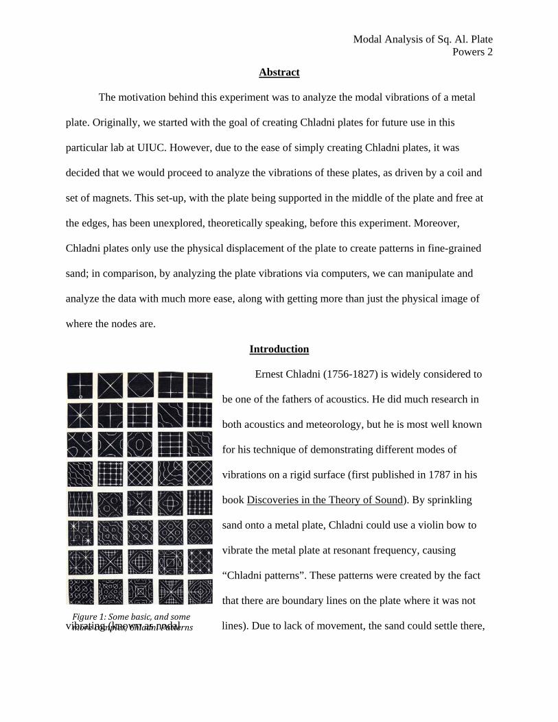
Ernest Chladni (1756-1827) is widely considered to
be one of the fathers of acoustics. He did much research in
both acoustics and meteorology, but he is most well known
for his technique of demonstrating different modes of
vibrations on a rigid surface (first published in 1787 in his
book Discoveries in the Theory of Sound). By sprinkling
sand onto a metal plate, Chladni could use a violin bow to
vibrate the metal plate at resonant frequency, causing
“Chladni patterns”. These patterns were created by the fact
that there are boundary lines on the plate where it was not
vibrating (known as nodal lines). Due to lack of movement, the sand could settle there, Figure1:Somebasic,andsomemorecomplex,ChladniPatterns
Modal Analysis of Sq. Al. Plate Powers 3
while being pushed off of the vibrating areas, and observers could view the patterns of the nodes.
Chladni’s technique has been modified over the years, employing electronic signal generators
instead of violin bows to produce a more accurate and more easily adjustable frequency.
Furthermore, Chladni also came up with a simple equation to predict the nodal patterns that
would be found on vibrating circular plates and other objects.
In this experiment, a simple Chladni plate was constructed and then analyzed. Although
Chladni and many others have since come up with the mathematics behind different plates and
set-ups, this set-up (supported in the center and free along all edges) has been unexplored thus
far, making this experiment novel.
Materials and Methods
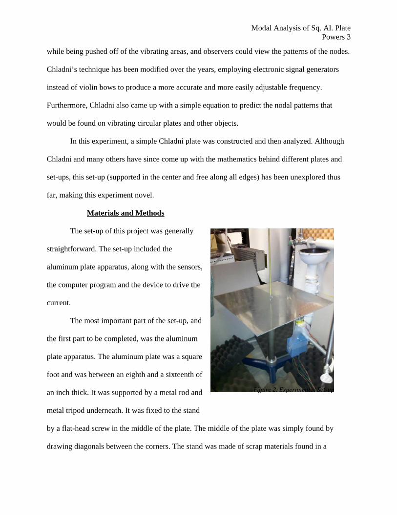
The set-up of this project was generally
straightforward. The set-up included the
aluminum plate apparatus, along with the sensors,
the computer program and the device to drive the
current.
The most important part of the set-up, and
the first part to be completed, was the aluminum
plate apparatus. The aluminum plate was a square
foot and was between an eighth and a sixteenth of
an inch thick. It was supported by a metal rod and
metal tripod underneath. It was fixed to the stand
by a flat-head screw in the middle of the plate. The middle of the plate was simply found by
drawing diagonals between the corners. The stand was made of scrap materials found in a
Figure2:ExperimentalSet‐up

Modal Analysis of Sq. Al. Plate Powers 4
storage room for UIUC physics laboratories. It was very important that when the plate was
screwed into the rod that it was as close to flat on the top as possible, so as to not interfere with
the sensors during the scanning. The hole in the middle of the plate was therefore angled outward
slightly, so that the screw could fit snuggly into the hole.
The plate was driven using a set of magnets and a coil underneath the plate. A pair of
magnets was placed in the same place, one on top of the plate and one below. The coil
underneath the plate then had an alternating current running through it. Taking advantage of the
changing current, the induced magnetic field then drove the set of magnets. Therefore, it was
fairly simple to control the frequency at which the plate was driven, by controlling the frequency
of the alternating current. The frequency was adjusted using a electronic signal generator in the
laboratory. There was only a small issue during the scans, due to the internal crystal (inside of
the signal generator) that controls the frequency and its lack of sensitivity, therefore inhibiting
our ability to get extremely accurate results. This was fixed by using an external device to
control the frequency and this solution provided us with much more precise results. The magnets
were placed at three different locations on the plates: at the corner, the center edge (meaning on
the center axis, but on the edge of the plate), or the quarter edge (still on the edge of the plate, but
halfway between the corner and the center axis of the plate).
There were two different sets of sensors for this experiment, one set above and on below.
The sensor above is labeled in the date as ‘Scan’, or just ‘S’, while the one below was ‘Monitor’,
or ‘M’.
The actual process of running the scans was extremely intensive and time consuming.
Each of the scans took somewhere between 4 and 8 hours each. Fortunately, the supervising
professor was gracious enough to run these scans for me. There were two different types of scans

Modal Analysis of Sq. Al. Plate Powers 5
that were performed. The first was just a general scan, in which the plate was driven at a variety
of frequencies, ranging from 0 Hz to 2000 Hz. The purpose o this type of scan was to find where
the resonant frequencies occurred. When a resonant frequency was reached, there was a sharp
peak, as seen in the graph below (the peaks are marked by a pinkish-purple open circle). A
narrow peak meant that the data was must more accurate and precise. As can be seen, the peaks
that were reached in the general scans were very promising. A computer program preformed the
variance the frequency.
Figure 3: General Scan plot, showing resonant frequencies, being excited from quarter-edge.
The second scan was a Mode-Locking Scan. The purpose of this scan was to stay as close
as possible to the resonant frequency. To do this, the imaginary part of the frequency is adjusted
so that the real part of the frequency stays as close to its maximum as possible (a more in-depth

explanati
seen in th
548.21 H
frequency
O
producin
Furtherm
number o
Unfortun
ion of mode-
he graph bel
Hz. The varia
y of 548 Hz
Over the past
ng hundreds o
more, there w
of resonant f
nately, there
-locking is a
ow, there is
ance is expec
only varied
Fig
t few months
of plots. On
were eight sep
frequencies t
is no way to
available in o
only slight v
cted in a mo
by .09 Hz is
gure 4: Mode-L
s, a tremendo
average, the
parate scans
that were ana
o properly di
other texts, b
variance in t
de-lock scan
s extremely
Locking plot ar
Results
ous amount
ere were 160
s in just the c
alyzed durin
iscuss all of t
Mo
but exceeds t
the frequency
n, and the fac
satisfying.
round 548 Hz.
of data has b
0 plots for ea
corner; the n
ng the time p
these graphs
odal Analysi
the depth of
y, between 5
ct that for th
been collecte
ach scan that
number eight
period of this
s in this pape
is of Sq. Al. Pow
f this paper).
548.12 Hz an
he resonant
ed and analy
t was run.
t was simply
s semester.
er, so I have
Plate wers 6
As
nd
yzed,
y the

Modal Analysis of Sq. Al. Plate Powers 7
chosen some plots and graphs that I feel are the most important to explain and talk about. Some
of the more interesting plots are below.
Figure 5: Real part of the Pressure, as collected from the Scanning sensor at 548 Hz.
Figure 6: Real part of the Impedance, as collected from the Scanning sensor, at 548 Hz.

Modal Analysis of Sq. Al. Plate Powers 8
Figure 7: Imaginary part of the Impedance, as collected from the Scanning sensor, at 548 Hz.
Figure 8: Real part of the wavelength (‘L’=Lamdba), as collected from the Scanning sensor, at 548 Hz.

Modal Analysis of Sq. Al. Plate Powers 9
Figure 9: Kinetic Energy, as collected by the scanning sensor, at 548 Hz.
Figure 10: Potential Energy, as collected by the scanning sensor, at 548 Hz.

Modal Analysis of Sq. Al. Plate Powers 10
Figure 11: Total Energy, as collected by the scanning sensor, at 548 Hz.
Figure 12: Imaginary part of the power density, as collected by the scanning sensor, at 548 Hz.

Modal Analysis of Sq. Al. Plate Powers 11
Figure 13: Depiction of the physical displacement of the plate, at 55 Hz, excited at the corner.
Figure 14: Depiction of the physical displacement of the plate, at 101 Hz, excited at the corner.
Discussion
Modal Analysis of Sq. Al. Plate Powers 12
The sheer amount of data and plots given after analysis was overwhelming. Information
included plots for impedance, energy, displacement, acceleration, pressure, and particle velocity.
For ease and brevity, most of the plots shown are from the set-up with the magnet at the corner
and at the resonant frequency of 548 Hz. Many of the plots are self-explanatory, so this section
will only discuss non-obvious, interesting aspects.
One of the most interesting aspects is that the plot of the real part of the impedance and
the plot of the real part of the wavelength are identical. Similarly, the likeness between the
kinetic energy, the total energy, and the imaginary part of the power density is striking.
Unfortunately, at this time, I do not know how to explain these two sets of similarities, but I
would hope that they would be explored in any furtherance of this experiment. Also, it should be
noted that only the imaginary part of the power density is shown above. This is due to the fact,
that mathematically, the real part of the power density actually equals zero.
One of the biggest issues for running the scans was the set-up being bumped while the
scans were running. There were extraneous vibrations that affected the mode-lock and general
scans, caused by both construction in the laboratory building and by janitors in the building
coming into the laboratory. This could be mostly fixed by placing the whole set-up into an
enclosed box, where no extra vibrations or change in air pressure could affect it. Also, there are
environmental issues that can affect what the resonant frequency is, such as room temperature.
Any slight change in room temperature affects the resonant frequency, and that is seen in the
variation of the frequency in the mode-locking scans.
In addition, there is a great amount of potential in the theoretical portion of this
experiment. Although there have been calculations regarding modal analysis of square plates,

Modal Analysis of Sq. Al. Plate Powers 13
there have not been previous calculations of this set-up, where the edges are free and the plate is
supported only in the center of the plate.
Conclusions
Generally speaking, this experiment was a great success, and the future of this project is
extremely bright and promising. There are many more experiments that could be done using the
Chladni plate constructed here.
One of the more obvious steps to be taken is to take a step back and use some type of
fine-grained salt to create physical patterns. This was tried once or twice this semester, but the
problem arose of the grains being too large, therefore being too heavy to be moved by the
vibrations of the plate. Adding sand has been attempted with other flat surfaces, such as a snare
drum head, but static electricity between the drumhead the sand prevented the patterns from
forming. Attempting to use sand to create physical nodal lines would be the next logical step for
this project.
Additionally, we recorded the sound of the vibrations made by the plate and analyzed
those; however, the analysis never went any further. This would also be a good way to go in the
future. It would be very interesting to see the resonant frequencies produced by a mallet hit and
compare those to the resonant frequencies of the driven vibrations.
Lastly, there is so much more to do in the computational field of this set-up. The
supervising professor has already produced some working equations for this set-up (which was
previously thought to be too difficult to solve) and those equations could be used in the future.
Overall, this project has a lot of potential for future experimentation over the next few
years, especially because of the novelty of the unsupported edges. There was a vast amount of

Modal Analysis of Sq. Al. Plate Powers 14
new information produced in only one semester and the amount that could be produced in the
upcoming semesters are very promising.