MOBILITY-BASED TOPOLOGY CONTROL OF ROBOT NETWORKS...
136
Transcript of MOBILITY-BASED TOPOLOGY CONTROL OF ROBOT NETWORKS...


MOBILITY-BASED TOPOLOGY CONTROL OF ROBOT NETWORKS
by
Sameera Poduri
A Dissertation Presented to theFACULTY OF THE GRADUATE SCHOOL
UNIVERSITY OF SOUTHERN CALIFORNIAIn Partial Fulfillment of the
Requirements for the DegreeDOCTOR OF PHILOSOPHY
(COMPUTER SCIENCE)
August 2008
Copyright 2008 Sameera Poduri

Dedication
This dissertation is dedicated to Amma, Nanna and Sundeep.
ii

Table of Contents
Dedication ii
List Of Tables v
List Of Figures vi
Abstract ix
Chapter 1: Introduction 1
Chapter 2: Related Work 82.1 Models . . . . . . . . . . . . . . . . . . . . . . . . . . . . . . . . . . . . . . . 92.2 Coverage Optimization . . . . . . . . . . . . . . . . . . . . . . . . . . . . . . . 122.3 Power Control for Network Connectivity . . . . . . . . . . . . . . . . . . . . . . 162.4 Network Configuration in three dimensions . . . . . . . . . . . . . . . . . . . . 182.5 Rendezvous . . . . . . . . . . . . . . . . . . . . . . . . . . . . . . . . . . . . . 18
Chapter 3: Local Geometric Conditions for Global Connectivity 213.1 Problem Formulation . . . . . . . . . . . . . . . . . . . . . . . . . . . . . . . . 243.2 Neighbor-Every-Theta (NET) Graphs . . . . . . . . . . . . . . . . . . . . . . . 25
3.2.1 Connectivity Analysis of NET Graphs . . . . . . . . . . . . . . . . . . . 273.2.2 Proximity Graphs . . . . . . . . . . . . . . . . . . . . . . . . . . . . . . 333.2.3 Coverage Analysis of NET Graphs . . . . . . . . . . . . . . . . . . . . . 40
3.3 NET graphs in three dimensions . . . . . . . . . . . . . . . . . . . . . . . . . . 433.4 Power Control with NET Graphs . . . . . . . . . . . . . . . . . . . . . . . . . . 463.5 Conclusions . . . . . . . . . . . . . . . . . . . . . . . . . . . . . . . . . . . . . 50
Chapter 4: Distributed Control Algorithms 524.1 Problem Formulation . . . . . . . . . . . . . . . . . . . . . . . . . . . . . . . . 534.2 Design of the Control Law . . . . . . . . . . . . . . . . . . . . . . . . . . . . . 544.3 Experiments and Results . . . . . . . . . . . . . . . . . . . . . . . . . . . . . . 59
4.3.1 k-degree Constraint . . . . . . . . . . . . . . . . . . . . . . . . . . . . . 604.3.2 NET constraint . . . . . . . . . . . . . . . . . . . . . . . . . . . . . . . 61
4.4 Conclusions . . . . . . . . . . . . . . . . . . . . . . . . . . . . . . . . . . . . . 66
iii

Chapter 5: Connectivity Maintenance and Coalescence 725.1 Problem Formulation . . . . . . . . . . . . . . . . . . . . . . . . . . . . . . . . 75
5.1.1 Communication Model . . . . . . . . . . . . . . . . . . . . . . . . . . . 755.1.2 Mobility Model . . . . . . . . . . . . . . . . . . . . . . . . . . . . . . . 765.1.3 Domain Model . . . . . . . . . . . . . . . . . . . . . . . . . . . . . . . 76
5.2 Coalescence Time Analysis . . . . . . . . . . . . . . . . . . . . . . . . . . . . . 775.2.1 Hitting Time . . . . . . . . . . . . . . . . . . . . . . . . . . . . . . . . 775.2.2 Meeting Time . . . . . . . . . . . . . . . . . . . . . . . . . . . . . . . . 785.2.3 Coalescence Time . . . . . . . . . . . . . . . . . . . . . . . . . . . . . 79
5.3 Simulation Results . . . . . . . . . . . . . . . . . . . . . . . . . . . . . . . . . 865.4 Conclusions . . . . . . . . . . . . . . . . . . . . . . . . . . . . . . . . . . . . . 87
Chapter 6: Coverage Optimization in Complex Environments 886.1 Problem Formulation . . . . . . . . . . . . . . . . . . . . . . . . . . . . . . . . 92
6.1.1 Partial derivative of the overall utility function . . . . . . . . . . . . . . 936.2 Distributed coverage control . . . . . . . . . . . . . . . . . . . . . . . . . . . . 94
6.2.1 Control Law for each sensor . . . . . . . . . . . . . . . . . . . . . . . . 946.2.2 Distributed Coverage Algorithm . . . . . . . . . . . . . . . . . . . . . . 956.2.3 Convergence . . . . . . . . . . . . . . . . . . . . . . . . . . . . . . . . 96
6.3 Deployment of Cyclops camera networks . . . . . . . . . . . . . . . . . . . . . 966.3.1 Sensing Performance Function . . . . . . . . . . . . . . . . . . . . . . . 966.3.2 Coverage Algorithm for 1D loop . . . . . . . . . . . . . . . . . . . . . . 1006.3.3 Simulation Results . . . . . . . . . . . . . . . . . . . . . . . . . . . . . 1036.3.4 Cyclops Experiments and Results . . . . . . . . . . . . . . . . . . . . . 109
6.4 Conclusions . . . . . . . . . . . . . . . . . . . . . . . . . . . . . . . . . . . . . 114
Chapter 7: Conclusions and Future Work 116
Bibliography 120
iv

List Of Tables
2.1 Classification of related work . . . . . . . . . . . . . . . . . . . . . . . . . . . . 20
4.1 Parameter values used in our implementation of the distributed deployment algo-rithm . . . . . . . . . . . . . . . . . . . . . . . . . . . . . . . . . . . . . . . . 64
v
List Of Figures
1.1 A network of 10 Create Robots deployed at USC . . . . . . . . . . . . . . . . . 2
1.2 Illustration of global connectivity of a robot network . . . . . . . . . . . . . . . 3
1.3 Illustration of global sensing coverage of a robot network . . . . . . . . . . . . . 4
2.1 Hexagonal arrangement of nodes for optimal coverage with (a) Overlaping disksand (b) Non-overlaping disks . . . . . . . . . . . . . . . . . . . . . . . . . . . . 14
3.1 Illustration of the NET condition . . . . . . . . . . . . . . . . . . . . . . . . . . 26
3.2 Proof of Theorem 3.2.6 for ‖ V1 ‖= 1 and ‖ V1 ‖= 2 . . . . . . . . . . . . . . . 29
3.3 Proof of Theorem 3.2.6 for ‖ V1 ‖= 3 . . . . . . . . . . . . . . . . . . . . . . . 30
3.4 A finite graph where all non-boundary nodes satisfy the NET condition . . . . . . 31
3.5 Degenerate cases of cuts through NET graphs that result in poor connectivity . . 33
3.6 RNG sector condition . . . . . . . . . . . . . . . . . . . . . . . . . . . . . . . . 34
3.7 θ = 2π3 bound for RNG . . . . . . . . . . . . . . . . . . . . . . . . . . . . . . . 37
3.8 Sector condition for GG . . . . . . . . . . . . . . . . . . . . . . . . . . . . . . . 38
3.9 Sector condition for DelG . . . . . . . . . . . . . . . . . . . . . . . . . . . . . . 39
3.10 Coverage with k nodes placed on the communication perimeter of node x . . . . 42
3.11 NET3D graph: each cone of angle θ must have at least one neighbor. . . . . . . . 44
3.12 RNG cone angle condition . . . . . . . . . . . . . . . . . . . . . . . . . . . . . 45
vi

3.13 Comparison of NET graphs and CBTC(α) for a uniform random network of 500nodes . . . . . . . . . . . . . . . . . . . . . . . . . . . . . . . . . . . . . . . . 49
3.14 Simulation results of power control based on NET graphs for a uniform randomnetwork of 500 nodes averaged over 100 runs . . . . . . . . . . . . . . . . . . . 50
4.1 Typical Network Configurations for a 64 robot deployment with k = 2 . . . . . . 67
4.2 Coverage and average degree for N = 49 and Rs = 4 for different values of Rc . 68
4.3 Variation of coverage with network size . . . . . . . . . . . . . . . . . . . . . . 69
4.4 Sample deployments with 100 robots and Rc = Rs = 8.0. . . . . . . . . . . . . 69
4.5 Sample deployments in the presence of obstacles with 100 robots andRc = Rs =8.0. . . . . . . . . . . . . . . . . . . . . . . . . . . . . . . . . . . . . . . . . . 70
4.6 Performance of the Distributed deployment Algorithms for a deployment of 100robots in terms of (a) Coverage, (b) Edge Connectivity (c) Average Degree and(d) NET condition satisfaction . . . . . . . . . . . . . . . . . . . . . . . . . . . 70
4.7 For θ ≤ 2π3 , the communication graph is a supergraph of RNG . . . . . . . . . . 71
5.1 Illustration of Coalescence for N = 5 . . . . . . . . . . . . . . . . . . . . . . . 74
5.2 Illustration of random direction mobility model . . . . . . . . . . . . . . . . . . 75
5.3 Verification of analytical model for kth meeting time . . . . . . . . . . . . . . . 79
5.4 Experimental validation of analytical bounds on Coalescence Time. The graphshows the coalescence time as a function of network size on a linear scale . . . . 82
5.5 Experimental validation of analytical bounds on Coalescence Time. The graphshows the coalescence time as a function of network size on a log scale . . . . . 83
6.1 (a) An aerial view of the garden (b) the pathway to be covered . . . . . . . . . . 89
6.2 Cyclops camera with an attached Mica2 Mote . . . . . . . . . . . . . . . . . . . 89
6.3 Node locations for (a) uniform deployment and (b) optimized locations and theirdetection results . . . . . . . . . . . . . . . . . . . . . . . . . . . . . . . . . . . 90
6.4 Perspective projection model . . . . . . . . . . . . . . . . . . . . . . . . . . . . 98
vii

6.5 Illustration of pixels on target not detected . . . . . . . . . . . . . . . . . . . . . 98
6.6 Validation of the proposed model for pixels detected vs. distance for three differ-ent environments . . . . . . . . . . . . . . . . . . . . . . . . . . . . . . . . . . 101
6.7 Performance of the distributed control law for three types of parameter functionson a 1D loop which is a 250 feet long smooth curve . . . . . . . . . . . . . . . . 104
6.8 Variation in coverage utility and convergence time for different network sizesaveraged over 50 iterations. . . . . . . . . . . . . . . . . . . . . . . . . . . . . . 105
6.9 Performance of the distributed control law in the presence of occlusions - (1)obstacles and (2) sharp corners. . . . . . . . . . . . . . . . . . . . . . . . . . . . 105
6.10 Performance of the distributed control law with partial knowledge of k1(x) andk2(x). . . . . . . . . . . . . . . . . . . . . . . . . . . . . . . . . . . . . . . . . 109
6.11 Cyclops setup . . . . . . . . . . . . . . . . . . . . . . . . . . . . . . . . . . . . 110
6.12 Performance of the distributed control law in an indoor rectangular corridor . . . 112
6.13 Performance of the distributed control law in an outdoor environment . . . . . . 113
viii

Abstract
A fundamental problem that arises in realizing large-scale wireless networks of mobile robots is that of
controlling the communication topology. This thesis makes three contributions to the area of mobility-
based topology control in robot networks.
First, this work proposes local, geometric conditions on robot positions that guarantee global network
connectivity. When combined with distributed controllers for mobile robots, these conditions maximize
sensing coverage while maintaining connectivity. The key idea is the introduction of a new construct -
a Neighbor-Every-Theta (NET) graph - in which each node has at least one neighbor in every angular
sector of size θ. We prove that for θ < π, NET graphs are guaranteed to have an edge-connectivity of at
least b 2πθ c, even with an irregular radio communication range. The NET conditions are integrated into an
artificial potential field-based controller for distributed deployment.
Second, for robots communicating over unreliable wireless links, a coalescence behavior is intro-
duced, in which disconnected robots recover connectivity by searching for others. Our contribution is an
asymptotic analysis of coalescence time which quantifies the trade-off between the cost of maintaining
connectivity and that of repairing connectivity - the first such guideline for designing controllers for robot
networks.
Finally, having shown how to construct and maintain robot networks with maximal coverage, we
address a problem motivated by the performance of cheap, low-resolution cameras in complex outdoor
environments. This variation of the sensor coverage problem is the first to address the case where the
sensing performance of each robot carrying a camera depends on the local environmental conditions. We
ix

present a distributed reconfiguration algorithm for this case, and validate it using a network of real Cyclops
cameras placed in environments with varying illumination and backgrounds.
x

Chapter 1
Introduction
Networked Robotics is emerging as a new frontier of Robotics. Groups of robots that are in-
dividually limited can use local communication to collectively achieve complex tasks involving
sensing and sharing of information, collaborative reasoning and inference, and manipulation.
Compared to traditional sensing technologies, the large-scale nature of these networks will allow
high-fidelity sensing over vast terrains and robustness to failures in the sensors. Further, such
networks can leverage mobility to adaptively configure in response to temporal changes in the
sensing field, application requirements, network properties, etc. Currently, several robots have
been designed, fabricated, and deployed as part of networked experimental testbeds. Examples
include the Robomote from the University of Southern California [Dantu et al., 2005], Swarm-
bot and Create (figure 1.1) from iRobot, Scout from the University of Minnesota [Hougen et al.,
2000], Alice and e-puck from EPFL [Caprari and Siegwart, 2005], and Scarab from the University
of Pennsylvania [Michael et al., 2008]. These deployments consist of 10 − 100 robots operat-
ing over short periods of time. Going by the rate of advancement in electronic fabrication and
communication abilities, we expect that in the near future swarms of several hundreds of robots
1

Figure 1.1: A network of 10 Create Robots deployed at USC. Each robot is equipped with aninfrared bump sensor, 802.11 wireless radio and an embedded computer.
will become available. Such systems will significantly change the way we interact with our sur-
roundings. Consider for example, a robot network being deployed in the aftermath of disasters
like hurricane Katrina to discover victims and provide communication infrastructure to rescue
teams, or aquatic networks in oceans to detect and mitigate harmful algal blooms or oil spills, or
a swarm of aerial robots that can track soldiers on a battlefield and form a routing network that
dynamically reconfigures in response to the communication requirements of the soldiers.
A fundamental challenge in realizing robot networks is developing algorithms that enable
intelligent behavior. Since the networks will be very large, the algorithms must necessarily be
de-centralized i.e. they must guarantee global behavior using only local information and local
control. Each robot can typically sense information (such as the relative positions of other robots
and obstacles) within a fixed range to itself and can communicate with robots that are close
to it. Using this limited information, it must decide its motion strategy such that one or more
global properties of the network (such as sensing coverage) are optimized and one or more global
network constraints (such as connectivity) are satisfied. This is an instance of the classic local-to-
global problem that arises in several complex systems. Coverage and connectivity are complex
2

(a) (b)
Figure 1.2: Network connectivity is a global property of robot positions. The filled circles arerobots and the black lines indicate communication links between pairs of robots. In (a) the net-work is connected. When the highlighted robot moves (b), it improves its local communicationlinks (dotted edges) but the global connectivity is broken.
functions of robot locations and controlling them through local interactions is not trivial. Con-
sider the example in figure 1.2, where the network is initially connected. The highlighted robot
moves and improves its local connectivity but in the process breaks one edge that results in the
network being disconnected. Similarly, even if each robot optimizes its local sensing coverage,
the network as a whole can have poor coverage (figure 1.3). The objective of this thesis is to
develop distributed algorithms for large-scale robot networks to maximize sensing coverage
while maintaining network connectivity.
The problem of maintaining the topological properties of networks is called topology con-
trol and has been studied extensively in the context of static and mobile ad-hoc networks such
as packet radio networks, vehicular networks, cell phone networks, and, more recently, sensor
networks [Santi, 2005]. In these networks, topology control can be achieved by varying the
transmission power of the radios (power control) and selectively turning nodes on or off (sleep
scheduling). The traditional approach is to assume that the network is connected when the radios
operate at full power (or all nodes are turned on) and find the minimum transmission power at
each node (or maximum number of nodes that can be turned off) while preserving the network
3

Figure 1.3: Sensing coverage is a global property of robot positions. The disk around each robotis its sensing range. Each robot choses a locally optimal location but the net coverage is far fromoptimal.
connectivity. Robot networks present a very different and interesting scenario for topology con-
trol. Unlike traditional static and mobile ad-hoc networks, robot networks allow control over
positions. Since connectivity properties directly depend on the positions of nodes, position con-
trol can be leveraged for effective topology control.
4

Our thesis is that
“Mobility can be effectively used for topology control of robot networks”
To establish the thesis, we present solutions to the following three problems:
1. Local conditions to guarantee global connectivity
We introduce Neighbor-Every-Theta (NET) graphs defined as graphs in which each node (except
those at the boundary) has at least one neighbor in every θ angular sector around it. Our key theo-
retical result is that for θ < π, a NET graph has an edge-connectivity of at least b2πθ c irrespective
of the edge-lengths. Based on these conditions we design a distributed navigation controller and
power controller. We implement a typical power control protocol using satisfaction of NET con-
dition at each non-boundary node as the termination criterion and show that a power-efficient
network with edge connectivity b2πθ c can be achieved even with realistic, irregular links.
We also present extensions of our results to 3D using a cone in place of the 2D sector. Topol-
ogy control in three dimensions (3D) is much more complex compared to 2D. As a result, there
is very little work on topology control algorithms in 3D. We propose an efficient algorithm for
identifying the largest empty cone of a node’s communication range. This algorithm can be used
in conjunction with several configurations mechanisms for implementing their 3D extensions.
2. Controllers for distributed deployment
We present a distributed algorithm for self-deployment of robot networks based on artificial po-
tential fields. The pair-wise interactions between the robots are govrened by two kinds of forces
- one causes the robots to repel each other to improve their coverage and the other is an attractive
5

force that restricts the inter-robot distances and thereby imposes local edge constraints. By using
a combination of these forces, every robot tries to maximize its coverage while maintaining local
constraints. Two types of constraints are considered - (1) minimum number of neighbors at each
robot and (2) NET condition. Simulations in Player/Stage simulation platform [Gerkey et al.,
2001] show that the controller achieves good sensing coverage and successfully maintains local
constraints even in the presence of obstacles.
The above potential fields based controller assumes that the network is initially connected.
To address the case where robots start in a disconnected state or accidentally lose connectivity
due to failures, we propose a ‘coalescing’ behavior where robots search for their peers and form a
connected network. We study the time taken for coalescence for a worst-case scenario where the
robots are memoryless (do not build a map) and do not have any knowledge of the environment or
positions of the other robots. Each robot performs an independent random search and when two
robots meet, they coalesce into a cluster and move together. Using the random direction mobility
model, we show that coalescence time has an exponential distribution which is a function of the
number of robots, speed, communication range, and size of the domain. Further, as the number of
robots (N ) increases, coalescence time decreases as O( 1√N
) and Ω( log(N)N ). Simulations validate
our analysis and also suggest that the lower bound is tight.
3. Coverage optimization in complex environments
We address a variation of the coverage problem for autonomous mobile sensors where the sens-
ing performance of each sensor depends on the local environmental conditions. We propose a
6

distributed control algorithm by which mobile sensors reconfigure their locations to provide op-
timal coverage. As an application we consider the problem of covering loopy pathways in indoor
and outdoor environments using cyclops camera. Local lighting conditions in these environments
significantly affect the sensing performance of each camera. Based on several experiments we
propose a location dependent sensing model for the camera. We present simulation results for
various scenarios and demonstrate convergence of our algorithm. We also present simulation
results on data collected in the indoor and outdoor settings.
Outline of Dissertation
The dissertation is organized as follows. The next chapter surveys related literature in geometric
optimization, sensor network topology control, and the Rendezvous problem in Robotics. Chapter
3 presents NET graphs and analysis of their connectivity properties in 2D and extensions to 3D.
Self-deployment algorithms for mobile nodes that maintain a local constraint are presented in
Chapter 4 followed by an analysis of Coalescence time in Chapter 5. In chapter 6, we describe
deployment in the presence of non-idealities in the sensor models. Finally, chapter 7 summarizes
the contributions and presents directions for future research.
7

Chapter 2
Related Work
The sensor coverage problem is related to classical geometric optimization problems such as disk-
covering, filling, voronoi partitions, set-cover [Hall, 1988], and the art-gallery problem [O’Rourke,
1987] and also the problem of multi-robot coverage [Gage, 1992]. The key factors that limit the
utility of the solutions of these problems to robot networks are 1) they do not provide for net-
work connectivity constraints and/or 2) they are centralized and assume global knowledge of
the domain. Not surprisingly, the sensor coverage problem has been an active research problem
in robotics. In this section, we review results from classical computational geometry as well as
those from recent research for location optimization in robot networks. The optimal locations can
be realized by using robots or humans to deploy networks [Batalin and Sukhatme, 2007; Corke
et al., 2004] or with networks of mobile robots [Howard et al., 2002; Cortes et al., 2004; Batalin
and Sukhatme, 2002]. In addition to controlling the locations of sensors, sensor coverage is also
studied in the context of sleep scheduling. Sleep scheduling techniques assume an initial high-
density deployment - the problem being to find the smallest subset of nodes that is sufficient to
provide the required coverage and connectivity. This is a discrete version of the sensor placement
8

problem - in the extreme scenario, if the sensor density is infinite, sleep scheduling is equivalent
to finding optimal sensor locations.
In the next section, we present an overview of the various models used for sensing, coverage
and communication. Later, we will discuss algorithms based on the models used (Table 2.1).
2.1 Models
Sensor Model
Let p = p1,p2, ...,pN,pi ∈ Q be locations of n sensors. The sensing performance of each
sensor i at point q is given by f(i,q). Depending on the nature of f(i,q), we can classify sensors
as follows:
• Isotropic Binary Disk Model: f(i,q) = 1 if ||pi − q|| ≤ Rs(i), and 0 otherwise. Rs(i)
is called the sensing range of sensor i. e.g. ranging sensors, temperature, acoustic, radio,
omnidirectional cameras, etc.
• Isotropic Continuous Model: f(i,q) = g(||pi − q||) where g is a monotonically de-
creasing, continuous function.
• Visibility Model: f(i,q) = 1 if the line segment pq ⊆ Q, and 0 otherwise. Also called
line-of-sight sensors.
• Limited range, visibility Model: If θ1, θ2, ...θn are the orientations of the sensors, then
f(i,q) = 1 if (1) ||pi − q|| ≤ Rs(i), (2) angle(i,q) ≤ φi, and (3) pq ⊆ Q, and 0
otherwise. φi is the field-of-view of sensor i. e.g. ranging sensors, cameras, etc.
9

A point in the domain, q is set to be covered if it is within the sensing region of at least
one node, i.e., if f(i,q) ≥ α for at least one i, where α is an application-dependent coverage
threshold. Similarly, a point q in the domain is k−covered if it is simultaneously covered by k
nodes. For sensors (like temperature sensors) that measure at a point, the sensing range can be
interpreted as a measure of sampling granularity.
Coverage Definition
Depending on the application, the desired sensing coverage can be characterized in one of 3 ways
(extension of the taxonomy proposed in [Gage, 1992]):
1. Blanket Coverage:
(a) Max type: If Φ(q),q ∈ Q, is the event density function, find an arrangement of
sensors such that the number of event detections per unit time is maximized, i.e.
C =i=n∑i=1
∫Q
Φ(q).f(i,q)dq
is maximized. If Φ is constant on Q, this is equivalent to maximizing the net area
covered given n sensors.
(b) Complete type: Find the minimum number of sensors such that each point in the
domain is covered, i.e. ,
q ∈ Q|f(i,q) ≥ α, 1 ≤ i ≤ n ⊇ Q
10

2. Barrier Coverage: Find an arrangement of a barrier of static nodes that minimizes the
probability of a moving target penetrating an area undetected.
3. Sweep Coverage: Find a motion strategy for a group of mobile sensors such that the num-
ber of event detection per time is maximized or the number of event misses per area is
minimized. This can be treated as a moving barrier where the targets are static.
Robot network coverage is generally of the blanket type because most of the applications
involve gathering spatial data from the environment. In this work, we consider blanket coverage
optimization.
Communication Model
Wireless communication depends on relative positions of nodes, radio characteristics and envi-
ronmental conditions. The probability that a message from node i reaches node j can be repre-
sented as PRR(i, j). In general, PRR(i, j) 6= PRR(j, i).
• Binary Disk Model: PRR(i, j) = 1 if ||pi − pj|| ≤ Rc(i), 0 otherwise. Rc(i) is called
the Communication range of sensor i.
• Probabilistic Model: In real scenarios, PRR(i, j) is not binary due to non-idealities in-
troduced by hardware and wireless propogation channel. It can be estimated empirically as
a probability distribution. [Zhao and Govindan, 2003; Zuniga and Krishnamachari, 2004;
Cerpa et al., 2005; Lymberopoulos et al., 2006].
11

Connectivity Constraints
A network is said to be connected if there exists at least one path between any two nodes. If
there exist at least k paths between any two nodes, then the network is k−connected. Since
robot networks must mostly operate unattended, connectivity is a necessary requirement to ac-
cess information from the network. Sometimes k−connectivity is desirable for increased fault
tolerance.
Since our work deals with blanket coverage, we first present an extensive survey of blanket
coverage optimization algorithms categorized by the sensor models they use. Several of these
techniques do not address connectivity. In section 2.3 we look at topology control techniques for
a sensor network whose main focus is on maintaining connectivity. Lastly, we review rendezvous
algorithms for groups of mobile robots.
2.2 Coverage Optimization
Binary Disk Sensor Model
Given a domain, D, and disks of fixed radius, R, disk-packing is the problem of finding the
densest arrangement of non-overlapping disks. For simple domains without holes/obstacles, the
hexagonal arrangement (fig. 2.1(a)) is optimal [Williams, 1979]. This is the densest arrangement
of binary disk sensors such that the area covered per sensor is maximum. In the Disk Covering
problem, the disks can overlap and the problem is to find the minimum number of disks that cover
every point in D. Again, a hexagonal arrangement (fig. 2.1(b)) is optimal. If the communication
12

model is a disk with radius at least twice the sensing range, then disk covering implies connectiv-
ity [Xing et al., 2005; Zhang and Hou, 2005]. For Rc ≥ 2Rs, sleep scheduling protocols can be
based only on coverage and a node can be turned off if it does not cover any point that is already
covered by other sensors. For Rc < 2Rs, CCP [Xing et al., 2005] and OGDC [Zhang and Hou,
2005] present heuristics to decide if a node can be turned off. They improve the efficiency of the
network by decreasing the number of active nodes but it is not necessarily the optimal, i.e. the
configuration with the minimum number of active nodes.
Several algorithms have been proposed for dispersion of mobile sensors in unknown environ-
ments [Hsiang et al., 2002; Howard et al., 2002; Batalin and Sukhatme, 2002]. These algorithms
do not consider the connectivity constraint. Potential Field techniques for robot applications were
first introduced by Khatib [Khatib, 1986] and ever since have been used extensively to develop
elegant solutions for path planning. Social potential fields have been introduced for robot for-
mations [Reif and Wang, 1999]. The deployment algorithm we propose is an extension of the
potential field-based deployment algorithm proposed in [Howard et al., 2002] where coverage is
achieved as an emergent property of the system.
Continuous Disk Model
There is a rich body of literature on optimization of facility locations such as locations of mail-
boxes in a city. The problem is to find locations for a limited number of facilities, that provide a
service demanded by users, such that the average (or maximum) distance from the demand points
to the facilities is minimized. The facilities can be modeled as points, lines, circles, or polygons
and the distance metrics can be euclidean, geodesic, minkowski, etc. For the sensor coverage
13

(a) (b)
Figure 2.1: Hexagonal arrangement of nodes for optimal coverage with (a) Overlaping disks and(b) Non-overlaping disks
problem, we are interested in the setting with point-like facilities and euclidean distance metric.
The distance to the facility (or a function of it) gives us the sensor’s performance function, f ,
which is isotropic and monotonically decreasing. If the demand points are uniformly distributed
in the domain, the voronoi diagram [Okabe et al., 1992], of a given arrangement of facilities, par-
titions the domain by allocating each domain-point to its nearest facility. The voronoi partition
of an arrangement of sensors can be used to compute the maximal breach path [Megerian et al.,
2005] which is the path between two points that maximizes the minimum distance to any sensor.
For point-like facilities, the Centroidal Voronoi Partition minimizes the average distance to
the facilities [Du et al., 1999]. Llyod’s Method [Llyod, 1982] is an iterative technique to construct
Centroidal Voronoi Partitions. Given an initial arrangement of k points (or facilities), the Voronoi
cells are constructed and their centroids are used as the new locations. This process is repeated
until the locations coincide with the centroids. Llyods method has been implemented as a dis-
tributed algorithm for a group of mobile facilities where each facility computes its local voronoi
cell and moves towards the centroid [Drezner, 1995; Cortes et al., 2004, 2005]. A non-uniform
14

demand density function can also be incorporated into this framework so that the distribution of
sensors follows the density function. It has been shown that a local estimate of the density func-
tion suffices for this algorithm [Schwager et al., 2006]. A key drawback of these methods is that
they do not consider obstacles in the domain. The optimality and convergence is proved only for
cases without obstacles.
Visibility Model
With the recent development of inexpensive image sensors [Rahimi et al., 2005], large camera
networks will soon be possible. Optimal positioning of visibility sensors is a different instance
of the locational optimization problem because they require line-of-sight. The art-gallery prob-
lem [O’Rourke, 1987] is to find an arrangement of cameras (that have infinite range and 360o
field of view) that can (blanket) cover a given polygon. In 2D, this problem can be solved in
polynomial time even when the polygons have holes. However, finding the arrangement with a
minimum number of cameras is NP-hard [Aggarwal, 1984]. A similar problem is also addressed
in motion-planning for mobile robots, to find the shortest trajectory or large workspace such that
the robot has an unobstructed view of the target [Briggs and Donald, 2000]. The above algorithms
are centralized and do not consider network connectivity constraints.
Finite range, visibility Model
Many of the real world cameras and ranging sensors have both limited field-of-view and limited
range. Finding the smallest number of such sensors to cover an arbitrarily complex domain is a
very hard problem. Recently, a number of approximation algorithms have been proposed. The
15

solutions are either based on randomized approaches [Danner and Kavraki, 2000; Banos and
Latombe, 1998] or a decomposition of the domain into smaller convex polygons [Kazazakis and
Argyros, 2002]. All of these algorithms are centralized and to the best of our knowledge, a
distributed algorithm has not been proposed yet. Instead of repositioning cameras, configuring
the settings such as pan, tilt, and zoom of a static arrangement of cameras can lead significant
improvement in sensing coverage and can be achieved in a distributed manner [Kansal et al.,
2007].
2.3 Power Control for Network Connectivity
Topology Control is considered a canonical problem in static and mobile ad-hoc networks (see
[Santi, 2005] for a detailed survey). Power control algorithms deal with maintaining connectivity
and do not address the problem of sensing coverage. In Cone Based Topology Control (CBTC)
[Wattenhofer et al., 2005], every node divides the space around it into sectors of angle α and
increases its transmission power till in each sector it can reach a neighbor or till it reaches its
maximum transmission power. There are two key differences between CBTC and the NET based
structured deployment: (1) NET condition does not assume the existence of a connected graph
when nodes operate at full power but provide ways to construct such a graph and (2) In CBTC,
it is possible that a non-boundary node operating at full power does not have a neighbor in an
α sector while in a NET graph every non-boundary node must have at least one neighbor in
each θ sector. The largest sector angle that guarantees connectivity in case of the NET graph
is π [D’Souza et al., 2006] as against 5π6 in CBTC. Several authors have proposed pruning the
communication graph to proximity graphs such as the RNG, GG, and Yao Graphs as a way to
16

achieve desirable connectivity and sparseness properties. Jennings, et. al., present a distributed
algorithm for constructing an RNG [Jennings and Okino, 2002] where each node increases it’s
transmit power till its neighbors cover the 2π region around it. We show that to obtain an RNG it
is sufficient to have one neighbor in each 2π3 sector and present sector based conditions for other
proximity graphs. In a similar spirit, D’Souza, et al.,[D’Souza et al., 2006] have shown that if
each non-boundary node in a network has at least one neighbor in every π sector around it, the
graph is guaranteed to be connected and is also sparse. Bredin, et. al., [Brendin et al., 2005] have
recently proposed a network repair strategy that finds additional node locations required to ensure
k-connectivity in any given network. The algorithm is proven to be within a constant factor of
the absolute minimum number of additional nodes.
Since sensing coverage and network connectivity are both related to the spatial configura-
tion of nodes, the relation between the two has generated a lot of interest. It has been shown
that if the communication model is a disk with radius at least twice the sensing range, then disk
covering implies connectivity [Xing et al., 2005; Zhang and Hou, 2005; Tian and Georganas,
2005]. Miorandi and Altman [Miorandi and Altman, 2005] performed a probabilistic analysis
of the relationship between radio connectivity and sensing coverage assuming a random uniform
distribution of the nodes. Recently, sensor placement problem has been studied for non-ideal sen-
sor and communication models [Krause et al., 2006; Zhang and Sukhatme, 2007]. The proposed
algorithm uses a pilot deployment to gather data and build non-parametric probabilistic models
for sensing and communication which are then used to find optimal sensor locations.
17

2.4 Network Configuration in three dimensions
Coverage optimization in 3D is significantly more challenging that in 2D. In fact, most of the
related problems like sphere-packing, art-gallery, and voronoi tetrahedralization are extremely
complex in 3D. Not surprisingly, there have been few efforts to address 3D sensor network prob-
lems like geographic routing [Kao et al., 2005] and localization [Biswas et al., 2006]. In [Bahram-
giri et al., 2006], an algorithm has been presented to extend CBTC [Wattenhofer et al., 2005]. The
computational complexity at each node is O(d3log(d)) as against O(dlog(d)) in 2D, d being the
average node degree. XTC [Wattenhofer and Zollinger, 2004] does not use the disc assumption
or angular information; given an initially connected network in 3D, it can retain connectivity.
2.5 Rendezvous
Rendezvous is the problem of multiple mobile robots meeting at a point in an unknown environ-
ment. In Coalescence, the robots do not stay collocated but try to spread out. Several distributed
Rendezvous algorithms have been proposed. Some of these assume connectivity [Ando et al.,
1999; Lin et al., 2003]. If the communication graph is an RNG then rendezvous algorithms have
been proposed that can deal with partial communication loss over some of the links [Cortes et al.,
2006]. In the absence of connectivity, the robots can explore the environment building a map
of the landmarks [Roy and Dudek, 2001] where other robots are likely to visit. This is similar
in spirit to the Coalescence problem where the base station is a landmark whose location is un-
known. However, our focus is on forming a connected component while allowing the robots to
remain “spread out” so that the time for coalescence is reduced.
18

Several algorithms have been proposed to maintain connectivity of a wireless network [Za-
vlanos and Pappas, 2005; Spanos and Murray, 2004] given that the initial network is connected.
Coalescence algorithms complement these by providing a way to regain connectivity in the event
of failures. In [Porfiri et al., 2007], the variation in connectivity of a network of robots performing
random walks on a lattice has been analyzed. Recently, the role of mobility in increasing sensing
coverage of a network has been analyzed [Liu et al., 2005]. In particular, it has been shown that
the time taken to detect an intruder decreases in comparison to a static network. In delay tolerant
networks, mobile nodes are disconnected most of the time and communicate when they are within
communication range of each other. To study the routing delay, the motion of the mobile nodes
is modeled as a random mobility model. In both the above cases, achieving connectivity is not
the goal and the nodes continue moving after an intruder is detected or message is exchanged.
In random walks literature, a coalescing random walk refers to a system of particles that
coalesce when they hit other particles while performing a random walk [Dykiel, 2005]. Several
asymptotic properties such as the time for convergence have been analyzed. Here, a group of
coalesced particles is equivalent to one particle and this analysis does not capture the increase in
communication spread.
19

Reference Mechanism CoverageModel
Comm Model &Connectivity
Distributed Comment
Isotropic Binary ModelWilliams [1979] placement Blanket, Max.
typeNone No Optimal
Williams [1979] placement Blanket, Com-plete
None No Optimal
Howard et al.[2002]; Batalin andSukhatme [2002]
Mobile Blanket, Max.type
None Yes Heuristic
Zhang and Hou[2005]; Xing et al.[2005]
Sleep schedule Blanket, Com-plete
Binary disk & 1-Conn
Yes Heuristic
NET graphs placement Blanket, Max.type
Binary Disk &tunable k-Conn
Yes Heuristic
Isotropic Continuous ModelOkabe and Suzuki
[1997]placement Blanket; Max None No Sufficient
Du et al. [1999] placement Blanket; Max None Yes OptimalCortes et al.
[2004]; Schwageret al. [2006]
mobile Blanket; Max None Yes Optimal
Infinite Range VisibilityChvatal [1975];
Aggarwal [1984]placement Blanket; Com-
pleteNone No Heuristic
Finite Range VisibilityKazazakis and Ar-gyros [2002]
placement Blanket, Com-plete
None No Approximate
Gerkey et al. [2006] mobile Sweep None No HeuristicKansal et al. [2007] “motility” Blanket, Max
typeNone Yes Optimal
Probabilistic ModelKrause et al. [2006] placement random random No OptimalData-centricdeployment
placement random no Yes Locally Opti-mal
Table 2.1: Classification of related work. The entries in bold refer to our work.
20

Chapter 3
Local Geometric Conditions for Global Connectivity
Topology control for ad-hoc wireless and sensor networks has traditionally only dealt with uncon-
trolled deployments, where there is no explicit control on positions of nodes [Santi, 2005]. The
primary mechanisms proposed are power control and sleep scheduling. These methods involve
removing edges from an existing, well connected communication graph in order to save power
while ensuring that the resultant sub-graph preserves connectivity. Robot networks present a dif-
ferent and interesting scenario for topology control. Since connectivity properties directly depend
on the positions of nodes, position control can be leveraged for effective topology control. Tradi-
tional approaches are ill-suited in such scenarios since they are not designed to exploit control of
the motion and placement of the nodes.
We develop a general approach that supports traditional methods like power control and also
allows new designs for controlled deployments. Our main contributions are:
• a k-connectivity result, based on local conditions and independent of communication model
• topology control algorithms based on the k-connectivity result for a) power control with
static nodes, and b) distributed deployment of mobile nodes
21

• 3D extensions of 2D results and an efficient algorithm for topology control in 3D.
We define Neighbor-Every-Theta (NET) graphs in which each node (except those at the
boundary) have at least one neighbor in every θ sector of its communication range. Our key
theoretical result is that for θ < π, a NET graph has an edge-connectivity of at least b2πθ c irre-
spective of the communication model. This implies that the condition only depends on the angles
between the neighbors of each node and holds for arbitrary edge-lengths. This feature is par-
ticularly relevant for sensor networks using low-power radios that have irregular communication
range. For the special case with an idealized disk communication model, we derive conditions for
maximizing the sensing coverage area (defined as the total area sensed by at least one node) while
satisfying the k-connectivity constraint, and for obtaining proximity graphs such as the Relative
Neighborhood Graph. It should be emphasized that the NET condition is local since each node
only requires relative position information of its (communicating) neighbors.
NET graphs are naturally suited for distributed power control. We implement a typical power
control protocol using satisfaction of NET condition at each non-boundary node as the termination
criterion and show that a power-efficient network with edge connectivity b2πθ c can be achieved
even with realistic, irregular links. This is in contrast to the sector based topology control algo-
rithms in literature including CBTC [Wattenhofer et al., 2005; Li et al., 2001], that rely on an
idealized disk communication model to guarantee connectivity properties. In CBTC based power
control [Bahramgiri et al., 2006], for a network to be k-connected, each node must either have a
neighbor in every θ = 2π3k sector or operate at full power. Our results imply that a sector angle
of θ = b2πk c is sufficient for k-connectivity. A three times larger value of sector angle implies
a much lower power requirement. We present simulation results to establish this in Section VI.
22

Even though we do not consider sleep-scheduling mechanisms in depth, it is possible to think
of designs where densely deployed nodes make sleep/wake decisions in a distributed manner by
using local, pair-wise negotiations based on combinations of NET condition satisfaction and other
criteria.
Position control is ideal for obtaining topologies that are NET graphs. Given the properties
guaranteed by the NET condition, an external agent deploying a static sensor network can make
decisions on the best positions for deployment of new nodes based on the geometry of the existing
network. Self-deploying mobile nodes can use this condition to decide their motion strategy. We
present a distributed algorithm for self-deployment of mobile nodes to concretely demonstrate the
use of the local and geometric conditions to implement coverage and connectivity tradeoffs. The
algorithm involves achieving NET condition satisfaction through purely pair-wise negotiations
between neighbors. The performance of this algorithm is studied through an implementation on
the Player/Stage simulation platform [Gerkey et al., 2001]. Results illustrate the tunable tradeoff
between connectivity and coverage and show that the distributed algorithm can achieve approxi-
mations of some coverage-maximizing tiling structures that also satisfy NET conditions.
Topology control in three dimensions (3D) is much more complex. There are several oper-
ations that are common to a wide range of topology control algorithms that have increased and
sometimes prohibitively high complexity in 3D. Examples include obtaining angular information
of and ordering neighbors and checking for intersections of overlapping regions [Santi, 2005;
Zhang and Hou, 2005; Xing et al., 2005; Cortes et al., 2005]. As a result, there is very little work
on topology control algorithms in 3D. We argue that controlled deployment and NET graphs are
well suited for sensor networks in 3D and present extensions to our 2D results. We propose an
23

efficient algorithm for identifying the largest empty cone of a node’s communication range. This
algorithm can be used in conjunction with several deployment and topology control mechanisms
for implementing their 3D extensions.
This chapter is organized as follows. The next section defines the problem and section 3.2
presents NET graphs and analysis of their connectivity properties which are extended to 3D in
section 3.3. Sections3.4 presents application of NET graphs for distributed power control respec-
tively and conclude in section 3.5.
3.1 Problem Formulation
Local conditions that guarantee global network properties are the key to designing distributed
topology control algorithms. In particular, we study local conditions that guarantee global k-
edge-connectivity of the network. Once such conditions are found, they can be integrated with
controls available in order to design topology control algorithms. Further, it is important to
understand if the results can be extended to 3D networks in an efficient manner. A detailed
description of these three problems follows.
Problem 1: k-connectivity certificates
Given a network, find local geometric conditions between node positions that can guarantee
global k-edge-connectivity.
A graph is said to be k-edge-connected if at least k edges must be removed to disconnect
it Diestel [2000]. By Menger’s theorem, this is equivalent to saying that there exist at least
k edge-disjoint paths between any two nodes in the graph. The graph that we consider is the
24

communication network where two nodes are said to have an edge between them if they can
communicate. In this case, high edge-connectivity is desirable because it implies high fault-
tolerance and path diversity.
By ‘local’ we mean that each node only has information about positions of its communicating
neighbors relative to its own position. The global coordinates of nodes are not available. The con-
ditions we seek must be based only on this local information so that each node can independently
decide whether it satisfies the condition.
Problem 2: Topology control
How can the local geometric conditions for k-connectivity be integrated power control?
Given a static network of N nodes, how should they choose their communication power such
that the network is k-connected and the energy is minimized?
Lastly, we study the extension to networks in three dimensions.
Problem 3: 3D networks
Do the local geometric conditions for 2D networks extend to 3D networks?
3.2 Neighbor-Every-Theta (NET) Graphs
In this section, we will define Neighbor-Every-Theta graphs and show that they give us k-
connectivity certificates.
25

(a) (b)
Figure 3.1: Illustration of the NET condition. Filled circles are symmetric neighbors. In a) nodedoes not satisfy NET condition. It has one sector greater than θ with no neighbor. In b) nodesatisfies NET condition, the largest sector with no neighbors is smaller than θ.
Definition 3.2.1 The Neighbor-Every-Theta (NET) condition (Fig. 3.1) for a node embedded in
the 2D plane is defined as requiring at least one symmetric neighbor in every θ sector of its
communication range.
Nodes A and B are symmetric neighbors if A can communicate to B and B can communicate to
A.
For finite networks, nodes on the network boundary cannot satisfy such a condition. The
boundary of a network can be defined as a cycle of nodes such that every other node lies inside
the cycle [Kroller et al., 2006]. A node that does not belong to the boundary is called an interior
node.
Definition 3.2.2 A NET graph is one in which every interior node satisfies the NET condition for
a given θ.
26

We now analyze the connectivity and coverage properties of NET graphs. For large networks
where the number of boundary nodes is small compared to the network size, we show that NET
graphs have an edge connectivity of at least b2πθ c, independent of the communication model.
With the stronger assumption of a idealized disk communication model, NET graphs, for specific
values of θ, contain proximity graphs such as the Relative Neighborhood Graph (RNG). An upper
bound on the sensing coverage is shown to be obtained from a symmetric arrangement of nodes
and can be computed as a function of θ. NET graphs form a family of graphs based on the
single parameter θ - as θ becomes smaller, the graphs become denser with an increasing level of
connectivity.
3.2.1 Connectivity Analysis of NET Graphs
The edge-connectivity of any graph is at most its minimum node degree and can in general be ar-
bitrarily low irrespective of the node degree [Diestel, 2000]. For some special graphs, higher node
degree implies higher edge-connectivity. One example of such a graph is the random geometric
graph, where an average node degree of O(logN) (where N is the network size) guarantees an
edge-connectivity of 1 with high probability [Xue and Kumar, 2004]. It turns out that for em
NET graphs also there is relation between minimum node degree and edge-connectivity. In NET
graphs every interior node has a degree of at least b2πθ c. We will show that the edge-connectivity
is also at least b2πθ c (except in pathological cases where boundary nodes can be disconnected by
removing fewer edges). This means that the easiest way to disconnect a NET graph is to discon-
nect a single interior node by removing b2πθ c edges. We will now formally establish this property
27

by first considering the simple case of graphs that are very large so that edges close to the bound-
ary are not significant. An extreme case of such graphs are the “boundary-less” graphs defined
below. Later, we will analyze the impact of boundary nodes on connectivity.
Definition 3.2.3 A NET graph is boundary-less if every node satisfies the NET condition. For
θ < π, such a graph must span the entire 2D plane.
Definition 3.2.4 Given a graph G = V,E, a cut set is a set of edges E′ ⊆ E such that
G′ = V,E−E′ has more than one component. The edge-connectivity a graph, λ, is the size of
its smallest cut set, C. Note that if G is connected, C must divide it into exactly two components.
Definition 3.2.5 For a graph embedded in the Euclidean plane a cut is a curve that partitions
the graph into two or more components.
Theorem 3.2.6 For θ < π, a boundary-less NET graph has an edge-connectivity λ ≥ b2πθ c
Proof: Consider a NET graph G = V,E. Let C ⊆ E be the smallest cut set of G so that
λ =‖ C ‖. Let the two components of G′ = V,E−E′ be G1 = V1, E1 and G2 = V2, E2.
WLOG, ‖ V1 ‖≤‖ V2 ‖.
If ‖ V1 ‖= 1 then ‖ C ‖≥ MinDegree ≥ b2πθ c (Fig 3.2(a)). If ‖ V1 ‖= 2 then ‖ C ‖≥
2(b2πθ c − 1
)≥ b2π
θ c since θ < π (Fig. 3.2(b)).
Suppose ‖ V1 ‖> 2. Construct the convex hull, H1 of V1. Then H1 ⊆ V1. Define angle φi
at hi ∈ H1 as shown in Fig 3.3. There will exist at least 3 vertices1 hi such that φi > π i.e. ,
∠hi < π. WLOG, assume that φ1, φ2 and φ3 > π. Since G = V,E is a NET graph, for
i = 1, 2, 3, φi must contain ≥ bπθ c edges ∈ C. Therefore, ‖ C ‖≥ 3bπθ c ≥ b2πθ c. 2
1SinceH is a convex polygon, ∠hi ≤ π,∀i. Suppose all except 2 internal angles are = π, say 0 < ∠h1,∠h2 < πand ∠hi = π for i = 3, 4, ...k, where k is number of vertices of H , then
Pk1 ∠hi = ((k − 2)π + ∠h1 + ∠h2) >
(k − 2)π. Contradiction sincePk
1 ∠hi = (k − 2)π.
28

(a) ‖ V1 ‖= 1 (b) ‖ V1 ‖= 2
Figure 3.2: The filled circles and edges represent G1, dotted edges form the cut set C.
The above result holds for the general case where the graph has boundary nodes provided
the cut is completely in the interior of the network, i.e. if all the nodes in V1 satisfy the NET
condition. If on the other hand, the cut mostly consists of boundary edges then it is not inter-
esting because it is unlikely to impact network performance. Now consider cuts that intersect
the network boundary twice - when entering and leaving the graph (fig. 3.4(a)). WLOG, assume
that the cut is minimal in length i.e. it is the shortest curve corresponding to its cut set. The case
when the cut intersects itself is covered by the above theorem - the number of edges cut inside
the loop alone must be at least b2πθ c. Assume that the cut does not intersect itself and by way
of contradiction, that it disconnects the network by cutting less than b2πθ c edges. We will now
analyze the nature of such a cut and prove that away from the network boundary, the distance
along the cut between two consecutive edges must be less than Rc.sec(θ/2), where Rc is an
upper bound on the edge-length. This implies that away from the boundary the cut cannot be
longer than b2πθ c · Rc.sec(θ/2). If θ is not close to π this expression is bounded. For example,
for θ = 0.9π it is ≈ 13 ·Rc and for θ = 2π3 it is 6 ·Rc. For large networks, a “short” cut like this
29

Figure 3.3: ‖ V1 ‖≥ 3 The red nodes and edges represent G1, the dotted edges form the cut setC. The corresponding convex hull H is shown with solid black lines.
can only exist close to the boundary (fig. 3.5(a)) or if the boundary is “pinched” [de Silva et al.,
2005](fig. 3.5(b)).
Lemma 3.2.7 For θ < π, the length of a minimal cut between two consecutive edges in a
boundary-less NET graph is less than Rc · sec(θ/2).
Proof: Let L be the cut and l its length between two consecutive edges it cuts, say (u1, v1) and
(u2, v2) (figure 3.4(b)). Then l ≤ maxd(u1, u2), d(u1, v2), d(v1, u2), d(v1, v2), where d() is
the euclidean distance function. Let the node pair that leads to maximum distance be P1, P2.
Now P1 must have at least one neighbor in each of the two θ sectors adjoining−−−→P1P2. Let these be
Q1 at an angle 0 ≤ α1 ≤ θ and Q′1 at an angle 0 ≤ α′1 ≤ θ with−−−→P1P2. 0 ≤ α1 + α′1 ≤ θ < π.
WLOG, α1 < π/2. Similarly Q1 must have a neighbor Q2 at an angle α2 ≤ θ, and so on till
some Qm−1Qm intersects−−−→P1P2. Note that the point of intersection cannot be in between P1
30

(a) (b)
Figure 3.4: (a) A finite graph where all non-boundary nodes satisfy the NET condition. The thickcurved line L is a cut through the graph (b) L cuts polygons
and P2 because otherwise L would cut Qm−1Qm contradicting the assumption that (u1, v1) and
(u2, v2) are consecutive edges.
We have,
31

l = ‖P1P2‖
≤ r1 · cos(α1) + r2 · cos(α1 + α2 − π) + · · ·
+rm · cos(α1 + α2 + · · ·+ αm − (m− 1)π)
(where π/2 > α1 > α1 + α2 − π > · · ·
> α1 + α2 + · · ·+ αm − (m− 1)π) > −π/2)
≤ Rc(cos(α1) + cos(α1 + α2 − π) + · · ·
+cos(α1 + α2 + · · ·+ αm − (m− 1)π))
(where Rc is an upper bound on edge length)
≤ Rc((cos(α1) + cos(α1 + θ − π) + · · ·
+cos(α1 − (m− 1)(π − θ)))
(since cos is a concave function in [−π/2, π/2])
= Rcsin(m·(θ−π)
2
)· cos
(α1 + (m−1)·(θ−π)
2
)sin(θ−π
2
)≤ Rc
1cos(θ/2)
2
It must be emphasized that the connectivity result only needs the largest edge in the network to
be bounded and holds even for a non-ideal and irregular communication models. In the following
subsections, we present further interesting properties of NET graphs with a stronger assumption
of an idealized disk communication model.
32

(a) (b)
Figure 3.5: Degenerate cases of cuts through NET graphs that result in poor connectivity. (a) Acut close to the boundary (b) pinched boundary
3.2.2 Proximity Graphs
Proximity graphs such as the Relative Neighborhood Graph (RNG), Gabriel Graph (GG) and
the Delaunay Graph (DelG) have several properties such as connectivity, sparseness, efficient
network routes, etc. that make them desirable network topologies [Li, 2003; Jennings and Okino,
2002; Rajaraman, 2002; Santi, 2005]. We will now analyze conditions under which NET graphs
will contain these proximity graphs. Here we assume an idealized disk communication model
but allow each node to have a different communication range. Further, the number of boundary
nodes is assumed to be small compared to the network size. The analysis presented is non-trivial
since the edge-lengths in NET graphs are restricted by the communication range of nodes, while
in proximity graphs they depend only on the relative positions of nodes and very long edges are
possible.
The set of edgesE for various proximity graphs is defined as follows [Diestel, 2000]. In what
follows, we use the name and location of a node interchangeably.
33

Figure 3.6: RNG sector condition. a) The circle of radius d(x, y) > Rc subtends an angle of 2π3 at
x. The lune contains an area larger than a 2π3 sector. b) The limiting case, when d(x, y) = R(x).
Disk graph (DG(V,E,R)): The directed graph containing all outgoing edges of a node,
u ∈ V , not longer than R(u).
E = (u, v)|u, v ∈ V and d(u, v) ≤ R(u)
Given positive r ∈ R, let C(p, r) be the circle consisting of points whose distance from point
p is strictly less than r. Define the lune, denoted L(p, q), to be the intersection of two circles,
both of radius d(p, q), centered at these points, that is, L(p, q) = C(p, d(p, q)) ∩ C(q, d(p, q)).
34

Relative Neighborhood Graph (RNG(V)): The undirected graph containing an edge (u, v)
if there is no point w ∈ V that is simultaneously closer to both u and v. Equivalently, (p, q) is an
edge if L(p, q) ∩ V = ∅.
E = (u, v)|u, v ∈ V and ∃ no w ∈ V 3
d(u,w) < d(u, v) and d(v, w) < d(u, v)
Gabriel Graph (GG): The undirected graph containing an edge (u, v) if the disk whose
diameter is edge (u, v) does not contain any other points of V, that is, if C(u+v2 , d(u,v)
2 )∩ V = ∅.
E = (u, v)|u, v ∈ V and C(u+ v
2,d(u, v)
2) ∩ V = ∅
Delaunay Graph (DelG): The undirected graph containing an edge (u, v) if the Voronoi
regions of u and v have non-empty intersection. From the properties of Voronoi diagrams it
follows the edges of triangle (u, v, w) are in DelG(V ) if their circumcircle does not contain any
other points of V .
These graphs are hierarchically related:
RNG(V ) ⊆ GG(V ) ⊆ DelG(V ).
In the proofs that follow, we assume that each node, u, in the network has a communication
range R(u) so that the communication graph of the network is a disk graph. Our next step is to
find conditions under which the RNG of the network is contained in the communication graph.
35

This is equivalent to finding conditions under which no edge (u, v) of an RNG is longer than
either R(u) or R(v). The following theorem presents this condition. Later, we prove similar
results for the GG and DelG.
Theorem 3.2.8 If each node x ∈ V has at least one neighbor in every 2π3 sector of C(x,R(x)),
the communication graph is a supergraph of RNG(V ). Moreover, 2π3 is the largest angle that
satisfies this property.
Proof: Consider any node x ∈ V . Suppose x has at least one neighbor in every 2π3 sector of
C(x,R(x)). We first show that for any node y outside C(x,R(x)), the edge (x, y) /∈ RNG(V ).
The lune L(x, y) will contain a sector of at least 2π3 (Fig.3.6). By premise, ∃ a node in L(x, y).
This implies that RNG(V ) does not have any edges incident on x that are longer than R(x).
Next we show that for any node z ∈ V insideC(x,R(x)) such that d(x, z) > R(z) i.e. (x, z) ∈
DG(V,E,R) but (z, x) /∈ DG(V,E,R), the edge (x, z) /∈ RNG(V ). Since z also has a
neighbor in every 2π3 sector of C(z,R(z)) and d(x, z) > R(z), from the above argument
(x, z) /∈ RNG(V ).
Therefore RNG(V ) ⊆ DG(V,E,R(x)).
Now suppose a node x′ ∈ V ′ has two neighbors with a sector angle of 2π3 +δ (δ > 0) between
them (Fig.3.7). We can place a node y′ outsideC(x′, Rc) such that the edge (x′, y′) ∈ RNG(V ′).
Therefore, 2π3 is the largest angle for which this condition holds.2
We have shown that for θ ≤ 2π3 , NET graph contains the RNG assuming an idealized disk
communication model. We can prove a similar property for GG and DelG, except that in this case
the value of θ is a function of the distance to neighbors.
36

Figure 3.7: θ = 2π3 bound for RNG - L(x, y) is empty
Lemma 3.2.9 If each node x ∈ V has at least one neighbor in every θ = 2 arccos( rR(x)) sector
of C(x, r) (r ≤ R(x)), the communication graph is a supergraph of GG(V ). Proof:Consider a
node X and a node Y outside C(X,Rc). For any r ≤ Rc, let β be the angle subtended by the
intersection area C(X, r) ∩ C(X+Y2 , d(X,Y )
2 ) at X . From Fig.3.8 we have,
r
2=d(X,Y )
2cos(
β
2)⇒ β = 2 arccos(
r
d(X,Y )).
Since arccos is strictly decreasing in [0, 1] and d(X,Y ) ∈ (Rc,∞), the smallest angle subtended
is
θ = inf β = 2 arccos(r
Rc). (3.1)
Suppose x has at least one neighbor in every
θ = 2 arccos(r
Rc)
37

Figure 3.8: Sector condition for GG
sector of C(X, r). By definition, the edge (X,Y ) /∈ GG(V ) if
C(d(X,Y )
2,d(X,Y )
2, ) ∩ V 6= ∅. (3.2)
(3.2) is satisfied for any choice of Y if there is a node Z ∈ V in the θ sector of C(X, r). By
premise such a Z exists and hence the GG will not have any edge lengths greater than Rc. This
implies that GG(V ) ⊆ DG(V,E,Rc).2
Corollary 3.2.10 If a node x has at least one neighbor in every θ = 2 arccos( rR(x)) sector of
C(x, r) (r ≤ R(x)), the communication graph is a supergraph of DelG(V ). Proof: Consider
all circles passing through X and Y . The smallest is C(X+Y2 , d(X,Y )
2 ) and the largest are two
circles of infinite radius of which the straight line through X and Y is an arc. From Fig.3.9, it
38

Figure 3.9: Sector condition for DelG
can be seen that the intersections of these circles with C(X, r) subtend an angle which is at least
θ at X , where
θ = inf β = 2 arccos(r
Rc).
By premise, there is at least one node in every θ sector ofC(X, r). Therefore, every circle passing
through X and Y will contain another node. So,
1. there is no Z ∈ V such that the4XY Z ∈ DelG(V )
2. trivially C(X+Y2 , d(X,Y )
2 ) also contains another node.
By 1,2 and definition of DelG, the edge (X,Y ) /∈ DelG(V ). Since the choice of Y is arbitrary,
there are no edge lengths greater than Rc in the DelG. Hence DelG ⊆ DG(V,E,Rc).
In real networks, it is not possible for the boundary nodes to satisfy the conditions required
by the theorems. We show using simulated deployments (in section 4.3.2) that the assertions can
be validated in spite of these exceptions.
39

3.2.3 Coverage Analysis of NET Graphs
Having listed the conditions that guarantee global connectivity properties, we now turn to the
problem of maximizing coverage. We assume that all nodes have a idealized disk sensing model
with a sensing radius of Rs. Maximizing sensing coverage is equivalent to packing problem with
a constraint placed on the communication neighbors. This is a very hard problem given an irreg-
ular communication model and even harder to solve locally. Therefore, we make a simplifying
assumption that the communication model is also an idealized disk with a radiusRc for all nodes.
Suppose that in order to satisfy the NET sector conditions, a node must have k = b2πθ c neighbors.
From the node’s local perspective, all neighbors must be located on the perimeter of the commu-
nication range to maximize coverage. Intuitively, the nodes must also be placed symmetrically
on the perimeter. We prove this result for the special case when Rc = Rs.
Lemma 3.2.11 For Rs = Rc, the area coverage is maximized when the k ≥ 3 nodes are placed
at the edges of k disjoint 2πk sectors of C(x,Rc).
Proof: Consider a node x and k nodes y1, y2, ...., yk placed on the perimeter of C(x,Rc). Let
these nodes be placed in anticlockwise order at angles β1 = 0, β2, ...., βk respectively. Define
θi = βi+1 − βi, 1 ≤ i ≤ k − 1
θk = 2π − βk (3.3)
We need to find θi such that the total area covered by these k + 1 nodes is maximized. The open
disks of all nodes lie within C(x, 2Rc) and are tangent to this disk at exactly one point (Ti) each.
40

The disks of adjacent nodes i and i + 1 intersect at point Ii (and at X). The total coverage lies
between πR2c and 4πR2
c and is maximized when the areak∑i=1
TiIiTi+1 is minimum (Fig.3.10).
TiIiTi+1
= TiXTi+1 − IiYiTi − IiYi+1Ti+1 − IiYiXYi+1
= (2Rc)2 · θi2− 2R2
c ·θi2− 1
2(2Rc sin
θi2
)(2Rc cosθi2
)
= R2c(θi − sin θi)
k∑i=1
TiIiTi+1 = R2c(
k∑i=1
θ −k∑i=1
sin θi)
= R2c(2π −
k∑i=1
sin θi) (3.4)
The problem now reduces to finding maxk∑i=1
sin θi subject tok∑i=1
θi = 2π and 0 ≤ θi ≤ 2π. Since
sin is non-negative and concave in [0, π] and non-positive in (π, 2π], it follows that the solution
is θi = 2πk , 1 ≤ i ≤ k.2
For k = 3, 4, 6, it is possible to place nodes such that each node has its neighbors placed
symmetrically on its communication range. The resulting communication graph will be a tiling
of the space: hexagonal, square and triangle for k = 3, 4 and 6 respectively. In these cases,
since each node maximizes coverage locally, the total coverage of the network will also be the
maximized. For values of k other than 3, 4 and 6 such an arrangement is not possible since
the corresponding tiling structures do not exist. Therefore in these cases, the local condition
for optimizing coverage will not necessarily optimize global coverage. Due to their symmetry,
41
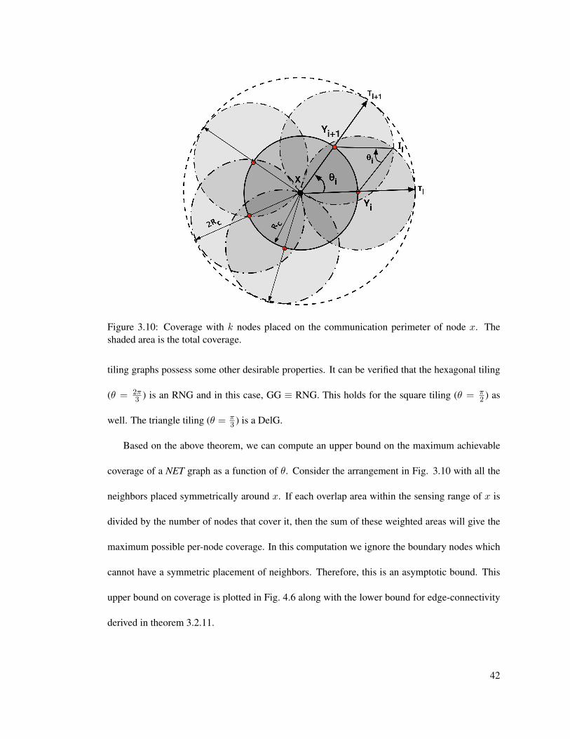
Figure 3.10: Coverage with k nodes placed on the communication perimeter of node x. Theshaded area is the total coverage.
tiling graphs possess some other desirable properties. It can be verified that the hexagonal tiling
(θ = 2π3 ) is an RNG and in this case, GG ≡ RNG. This holds for the square tiling (θ = π
2 ) as
well. The triangle tiling (θ = π3 ) is a DelG.
Based on the above theorem, we can compute an upper bound on the maximum achievable
coverage of a NET graph as a function of θ. Consider the arrangement in Fig. 3.10 with all the
neighbors placed symmetrically around x. If each overlap area within the sensing range of x is
divided by the number of nodes that cover it, then the sum of these weighted areas will give the
maximum possible per-node coverage. In this computation we ignore the boundary nodes which
cannot have a symmetric placement of neighbors. Therefore, this is an asymptotic bound. This
upper bound on coverage is plotted in Fig. 4.6 along with the lower bound for edge-connectivity
derived in theorem 3.2.11.
42

In the next section we extend NET graphs to 3D and study their connectivity and coverage
properties.
3.3 NET graphs in three dimensions
Network configuration in 3D is significantly more complex than in 2D. There are several oper-
ations that are common to a wide range of sensor network configuration algorithms in 2D that
have increased and sometimes prohibitively high complexity in 3D. We argue that controlled
deployment and NET graphs are well suited for sensor networks in 3D and present extensions
to our 2D results. We propose an efficient algorithm for identifying the largest empty cone of a
node’s communication range. This algorithm can be used in conjunction with a number of generic
deployment and topology construction mechanisms for implementing their 3D extensions.
A node satisfies the NET3D condition if it has at least one symmetric neighbor in every cone
of solid angle θ. A NET3D graph is one in which every node except those on the boundary satisfy
the NET3D condition. If the network is very large compared to the size of its boundary, we make
the following conjecture for the edge-connectivity.
Conjecture 3.3.1 For θ < 2π, a boundary-less NET3D graph has an edge-connectivity λ ≥
b2πθ c 2
Note that, like in 2D, the connectivity result is independent of the communication model. For
specific values of θ, NET3D graphs will contain proximity graphs such as RNG, GG, and DelG.
Lemma 3.3.2 If each node x ∈ V has at least one neighbor in every θ = π cone of S(X,R(x)),
the communication graph is a supergraph of RNG(V ).
43

Figure 3.11: NET3D graph: each cone of angle θ must have at least one neighbor.
Lemma 3.3.3 If each node x ∈ V has at least one neighbor in every θ = 2π(1 − rRc
) cone
of S(X,R(x)), the communication graph is a supergraph of GG(V ) and DelG(V ). Moreover,
2π(1− rR(x)) is the largest angle that satisfies this property.
The proofs follow from the corresponding proofs in 2D and the fact that a cone with apex
angle α will contain a solid angle of θ = 2π(1− cos(α)). For example in the proof for RNG, the
3D lune will contain a cone with apex angle α = 2π3 and solid angle of θ = π.
Algorithm to check NET condition
The local conditions described above can be integrated with node placement to construct efficient
topologies. A key requirement is an algorithm to check for empty cones larger than a given θ.
44

Figure 3.12: RNG cone angle condition
For instance, to check for formation of RNG, θ = π. This step is non-trivial in 3D because there
exists no natural “order” of neighbors. We propose the following algorithm for finding the largest
empty cone around a given node.
Algorithm 1: largestCone(G = (V,E),v ∈ V )
let S be the unit sphere centered at v
for each u ∈ Neighbor(v), let −→vu be the
direction vector from v to u
let cu be the intersection of −→vu with S
let DT be spherical delaunay triangulation cu∀u
find ai,j,k = area of circumcircle of triangle
(ui, uj , uk) ∈ DT
return max(ai,j,k)
Algorithm 1: Find largest empty cone around a node
45
Theorem 3.3.4 For a given graphG = (V,E) and node v, largestCone returns the largest empty
cone around v.
Proof: The circumcircle of every (spherical) triangle in the spherical delaunay triangulation is
empty [Na et al., 2002]. Therefore the cone returned by largestCone is certainly empty. Suppose
there exists an empty cone (whose image on the unit sphere is the circle c) that is larger than
the one returned by largestCone. Then the center of c lies in some triangle t of the delaunay
triangulation. Since c is empty, none of the vertices of t must lie inside c. This implies that the
circumcircle of t will be larger than c which is a contradiction. Therefore largestCone correctly
returns the largest empty cone.2.
The computational complexity of largestCone isO(dlog(d)) where d is the number of neigh-
bors of a node. This is because, the complexity of spherical triangulation is O(dlog(d)), the
number of triangles generated is O(d), and sorting them will also take O(dlog(d)) time.
Several topology control algorithms [Santi, 2005; Wattenhofer et al., 2005; Jennings and
Okino, 2002; Xing et al., 2005; Zhang and Hou, 2005] in 2D rely on directional information and
in particular use the angle between adjacent neighbors. This algorithm can be used as a primitive
for extending such algorithms to 3D.
3.4 Power Control with NET Graphs
In this section we illustrate how NET graphs can be used for topology control of a static network
by varying the communication power. The result is a power control mechanism that can guaran-
tee k-edge-connectivity without any restriction on the communication model. In contrast, most
46

existing power control algorithms, including the well-known CBTC [Wattenhofer et al., 2005;
Bahramgiri et al., 2006] algorithm, require an idealized binary disk communication model.
In the power control problem, we are given a network deployed with a sufficiently large
density so that connectivity (k-connectivity) is guaranteed when nodes operate at full power. The
objective is to find an assignment of transmission powers to nodes so that the reduced graph
retains connectivity (k-connectivity) while expending minimum energy. In some applications
it is also desirable to maintain other properties such as planarity, sparseness, spanner, etc. NET
graphs are naturally suited for distributed power control because
• they are based on local geometric conditions that guarantee global k-connectivity,
• communication range for the low power radios used in sensor network applications is
highly irregular [Zhao and Govindan, 2003; Zuniga and Krishnamachari, 2004]. The con-
nectivity properties of NET graphs are independent of the communication model.
Consider a sensor network such that when nodes operate at full power, they satisfy the NET
condition for a given θ. Using a typical power control protocol and satisfaction of NET condition
at each internal node as the termination criterion, a power-efficient k-connected network can be
achieved.
We have implemented a completely distributed power control algorithm as follows. Starting
with a minimum value, each node incrementally increases its transmission power till the NET
condition is satisfied. We assume that the orientation of neighbors can be computed either from
angle-of-arrival of messages or localization information. Each node computes its empty sectors
and increments power if 1) NET condition is not satisfied or 2) if it has an asymmetric incoming
link from a node that does not satisfy NET condition. Since boundary nodes (detected using
47

an algorithm such as [Kroller et al., 2006]) are not required to satisfy NET condition, they only
increase power in response to incoming asymmetric links. This is a simple implementation with
scope for further power optimization which we plan to pursue in future. Our objective here is
to demonstrate that for a given θ the resulting topologies preserve b2πθ c edge-connectivity. In
simulations, we used realistic statistical models for wireless links developed in [Zuniga and
Krishnamachari, 2004] for which the authors have made code available online [Zuniga et al.,
2005].
Fig. 3.4 shows typical topologies resulting with 500 nodes distributed uniformly at random
on a 80m x 80m square. Nodes that cannot satisfy the NET condition at full power are identified
as boundary nodes (shown as red squares). The initial transmission power was set to −10dB
and incremented in steps of 1dB. Links that had a packet reception rate of at least 90% were
considered active. Note that the figures only show bidirectional links. The simulations were
terminated when all non-boundary nodes satisfied NET condition.
Fig. 3.4 (a) and (b) show the comparison the topologies resulting from NET based power
control and CBTC(α) [Bahramgiri et al., 2006] for 2-edge-connectivity. According to CBTC(α)
a node must either have a neighbor in every θ = 2π3k or operate at full power to guarantee k-
edge-connectivity. We show that having a neighbor in every θ = 2πk is sufficient to guarantee
k-edge-connectivity. As a result, NET condition results in a significantly sparser, and hence
efficient, topologies compared to CBTC(α).
Fig. 3.14 shows the edge-connectivity and average power over 100 iterations. Edge-connectivity
was computed as the minimum number of paths consisting of symmetric links between any two
internal nodes. In all experiments, the edge-connectivity was always greater than b2πθ c. This
48

validates our key theoretical result, Theorem 3.4. The average power used increases quickly as θ
decreases (fig. 3.14(b)). This implies that for efficient topology control it is important to choose
the largest value of θ possible depending on the application requirements. Because NET graph
requires an angle (θ = 2π/k) that is three times bigger than the angle required by CBTC(α)
(θ = 2π/3k), the power saved will very large. For example, for 2-edge-connectivity, CBTC(α)
requires an average power of 4dB while NET graph requires −6dB.
These initial results are promising because we are able to achieve power-efficient topologies
that guarantee k-connectivity through distributed power control even with realistic, irregular link
models.
(a) θ = π (b) θ = 2π6
Figure 3.13: Comparison of NET graphs and CBTC(α) for a uniform random network of 500nodes. For 2-edge-connectivity, (a) NET graph requires sector angle θ = π and average power−5.91dB while (b) CBTC requires θ = 2π
6 and average power of 4.10dB.
49

(a) edge-connectivity (b) average power
Figure 3.14: Simulation results of power control based on NET graphs for a uniform randomnetwork of 500 nodes averaged over 100 runs. The edge-connectivity is greater than the 2π
k lowerbound derived in Theorem 3.4. The average communication power for achieving 2-connectivityusing CBTC(α) is 4dB (red square) compared to −6dB using NET graphs.
3.5 Conclusions
This chapter addresses distributed topology control using a construct called Neighbor-Every-
Theta (NET) graphs. These graphs have the following two properties that allow for simple and
practical algorithm design:
• tunable connectivity based on a single parameter, the sector angle θ
• connectivity guarantees do not depend on communication model
NET graphs are such that each node has at least one neighbor in every θ sector around it.
We prove that for a given θ < π, NET graphs have an edge connectivity of at least b2πθ c, except
in pathological cases where the network can be partitioned close to its boundary. This property
holds even in cases when the communication model is irregular. For the special case of an ide-
alized disk communication model, it is shown that for specific values of θ, NET graphs contain
50
proximity graphs such as the relative neighborhood graphs that are well known to be desirable
communication topologies. We also prove the symmetric neighbor placement condition for max-
imizing sensing coverage under the NET condition.
To concretely demonstrate the use of NET graphs for tunable power control, we implement
a typical protocol using satisfaction of NET condition at each internal node as the termination
criterion and show that a power-efficient network with edge connectivity 2πθ can be achieved even
with realistic, irregular links.
Lastly, we consider NET graphs in three dimensions and study their connectivity properties.
It is our conjecture that for a given solid angle θ < 2π, NET3D graphs have an edge connectivity
of at least b4πθ c when partitions close to the boundary are ignored. There is very little earlier
work on topology control in 3D. Several geometric computations become complex and even
intractable when extended from 2D to 3D. We have developed an efficient algorithm for deter-
mining the largest empty cone around a node in 3D based on spherical Delaunay triangulations.
The running time is O(dlogd) for average node density d, which is a significant improvement
over the earlier O(d3logd) algorithm proposed in the context of CBTC [Bahramgiri et al., 2006].
The new algorithm can be used to extend several sector based topology control algorithms to 3D.
Topology control in 3D is an important area for further research.
In the next chapter, we develop distributed deployment algorithms for robot networks to
achieve NET conditions.
51

Chapter 4
Distributed Control Algorithms
In this chapter we propose deployment algorithms for robot networks that maximize sensing
coverage while maintaining a local constraint. We consider two constraints
1. k−degree: each robot has degree at least k where k is a parameter to the algorithm
2. NET condition: each robot satisfies the NET constraint, i.e. has at least one neighbor in
every θ sector of its communication range, where θ is a parameter to the algorithm.
We assume that the robots do not have global localization or a global map of the environment
but can sense the distance and orientation of their neighboring robots.
Our approach is based on virtual potential fields. We treat each robot in the network as a vir-
tual charged particle and define simple force laws to govern the interaction between neighboring
robots. These laws incorporate two different kinds of forces. One is a repulsive force that tries to
maximize coverage while the other is an attractive force that imposes the local constraint. As a
result of these forces, a group of robots placed close together spreads out into a network to maxi-
mize the coverage while satisfying the local constraint. The deployment proceeds by starting in a
state where all the constraints are satisfied and at each step robots move such that no constraints
52

are broken. In the next chapter, we consider the case where the robots are disconnected at the
start of deployment.
4.1 Problem Formulation
Problem: Given N mobile robots with isotropic radial sensors of range Rs and isotropic radio
communication of range Rc, how should they deploy themselves so that the resulting configura-
tion maximizes the total sensor coverage of the network while maintaining a local constraint at
each robot?
We make the following assumptions:
1. The robots have isotropic binary disk sensing and communication,
2. The robots are capable of omni-directional motion, and
3. Each robot can sense the exact relative range and bearing of robots within its sensing range
We impose certain desiderata on the problem solution. The deployment algorithm should:
• be distributed and scalable
• not require a prior map or localization of robots
• adapt to changes in the environment and the network itself
We use the following three metrics to evaluate the performance of the deployment algorithm.
1. the normalized per-robot coverage. This is defined as:
Coverage =(Net Area Covered by the Network)
NπR2s
53

In the remainder of the chapter, we use the term ‘coverage’ to mean the normalized per-
robot coverage as defined above.
2. the percentage of robots in the network that satisfy the local constraint, and
3. the average degree of the network.
4.2 Design of the Control Law
Potential field-based techniques have been used extensively to solve navigation problems in mo-
bile robotics. In these methods, virtual potential fields are used to represent goals and constraints
and the control law for the robot’s motion is formulated such that it moves from a high potential
state to a low potential state similar to the way in which a charged particle would move in an
electrostatic field.
In our deployment algorithm, we construct virtual forces between robots so that each robot
can attract or repel its neighbors. The forces are of two kinds. The first, Fcover, causes a pair of
robots to repel each other to increase their sensing coverage. The second, Fconstraint constrains
a pair robots by making them attract each other when they are on the verge of being disconnected.
By using a combination of these mutually opposing forces, each robot maximizes its coverage
while maintaining the local constraint. The deployment proceeds by starting in a state where all
the constraints are satisfied and at each step robots move such that no constraints are broken.
A robot whose constraints are fully satisfied, repels all of its neighbors using Fcover till its
local constraint is about to be broken. The resulting neighbors are called the robot’s critical
neighbors and the connections between them and the robot are called critical connections. The
54

robot now communicates to all its critical neighbors that its connection with them is critical and
therefore should not be broken. It then continues to repel all its neighbors using Fcover but
as the distance between the robot and its critical neighbor increases, ‖Fcover‖ decreases and
‖Fconstraint‖ increases. As a result, at some distance ηRc, where 0 < η < 1, the net force
‖Fcover + Fconstraint‖ between the robot and its neighbor is zero. At this distance, the robot
and its neighbor are in equilibrium with respect to each other. We call 1η the safety factor because
the larger its value, the smaller the probability of critical neighbors losing connectivity.
The forces are constructed as inverse square law profiles - ‖Fcover‖ tends to infinity when
the distance between robots is zero so that collisions are avoided. Similarly, ‖Fconstraint‖ tends
to infinity when the distance between the critical neighbors is Rc so that loss of connectivity
between them is prevented.
Mathematically, the forces can be expressed as follows. Consider a network of n robots
1, 2, 3, . . . , n at positions x1,x2, . . . ,xn respectively. Let ∆xij represent the Euclidean distance
between robots i and j, i.e. ∆xij = ‖xi − xj‖
Fcover and Fconstraint are defined as follows.
Fcover(i, j) =(−Kcover
∆xij2
)(xi − xj
∆xij
)
Fconstraint(i, j) =
Kconstraint
(∆xij−Rc)2
(xi−xj
∆xij
)if critical connection;
0 otherwise.
where Kcover and Kconstraint are the force constants.
55

The resultant force between the robots i and j is
F(i, j) = Fcover(i, j) + Fconstraint(i, j)
and robot i will experience a net force of
Fi =∑
all neighbors j
F(i, j)
The equation of motion for robot i is formulated as:
xi(t) =(
Fi − νxi
m
)
where ν is a damping factor and m is the virtual mass of the robot which is assumed to be 1.
Computational Details
Having described the equation of motion for the robot, we discuss our choices of the four param-
eters Kcover, Kconstraint, ν and η.
• Kcover: Consider two robots that are repelling each other. As the distance d between them
increases, the combined coverage of the robots increases, reaches a maximum of 2πR2s at
d = 2Rs and remains constant after that. This implies that for d > 2Rs repelling does not
improve coverage. We therefore pick a value for Kcover such that at
d = 2Rs, ‖Fcover‖ ≈ 0
56

• Kconstraint: At d = ηRc we want ‖Fcover + Fconstraint‖ = 0, i.e.
−Kcover
η2Rc2 +
Kconstraint
(η − 1)2Rc2
= 0
Kconstraint =(1− η)2
η2Kcover
• η: A large η increases the probability of critical neighbors getting disconnected while a
small η results in lesser coverage. We used a value of 0.8 for η. This is a heuristic choice
based on experimental experience.
• ν: We conducted a simple ‘two-body’ variant of our scenario by implementing our algo-
rithm on two robots to study the variation in their interaction for different values of ν. For
these experiments we fixed the values of Kcover, Kconstraint and η as explained above. We
found that for small values of ν the system oscillates. We picked the smallest value of ν that
does not lead to oscillations. This value corresponds roughly to the critically dampedcase
for our system. In our experiments, we used ν = 0.25.
In the following, we analyze the coverage achievable by uniform random and symmetrically
tiled network configurations that satisfy the constraint of k-degree. These will serve as reference
points to evaluate the performance of our algorithm.
Coverage of Uniform Random Networks
A uniform random network is one in which the robots are distributed randomly and with a uniform
density. For such networks, the probability of finding i robots in a specified domain depends only
57

on the area of the domain and not on its shape or location. Given any area S, the probability that
it will contain exactly i robots is given by
P (i) =(ρS)i
i!e−ρS
where ρ is the density of robot deployment [Hall, 1988].
The probability that a randomly chosen robot will have a degree of at least k is the probability
that there will be at least k robots in the area πR2c around it.
P (i ≥ K) = 1−i=(K−1)∑i=0
(ρπR2c)i
i!e−ρπR
2c
As the density of deployment increases, the probability that each robot will have a degree
of at least k, increases but the per-robot coverage of the network decreases. Therefore the best
coverage achieved by a random network that satisfies the constraint of k-degree with a high
probability, say 0.95, will correspond to the smallest density for which P (i ≥ K) ≥ 0.95. Let
this density be ρ′.
The coverage of a uniform random network is a function of its density and Rs. For a network
with density ρ′ the normalized per robot coverage is:
Coverage =1− e−ρ′πR2
s
ρ′πR2s
Note that this expression is independent of the number of robots in the network.
58
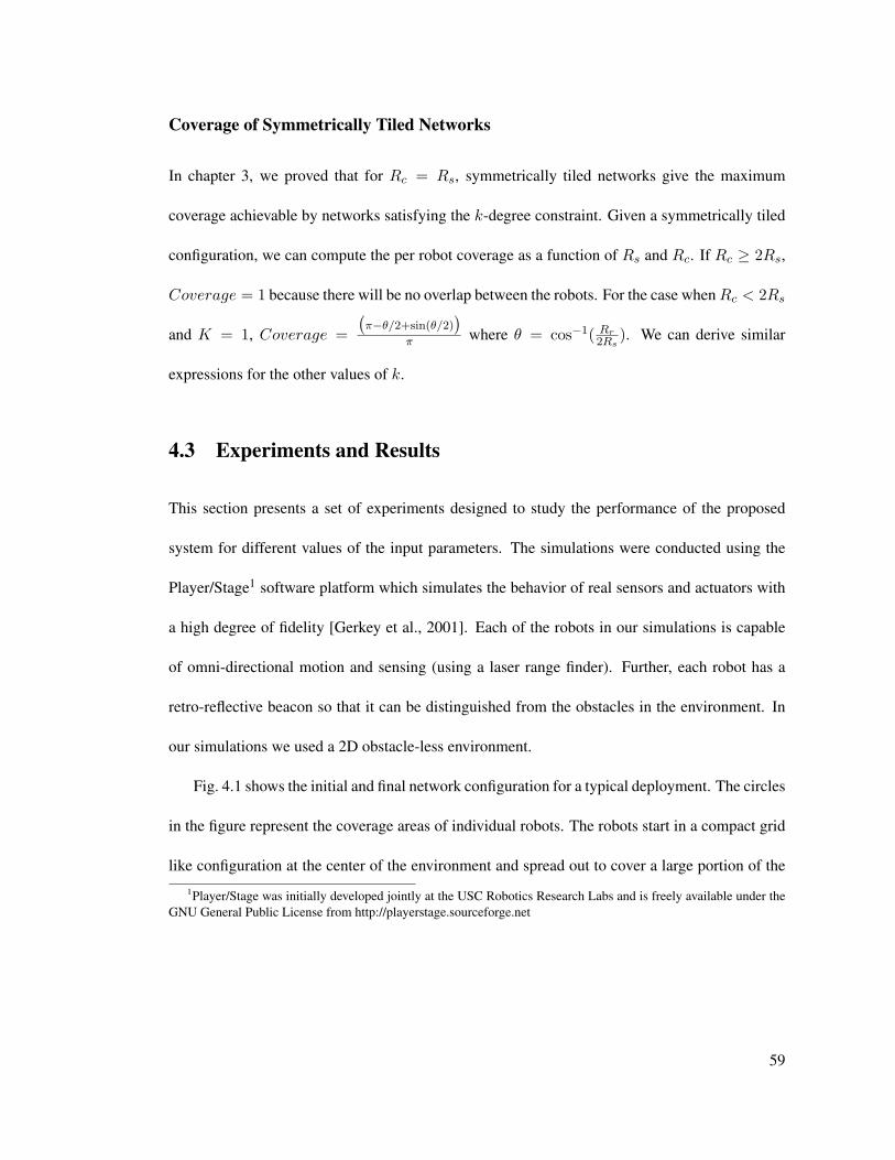
Coverage of Symmetrically Tiled Networks
In chapter 3, we proved that for Rc = Rs, symmetrically tiled networks give the maximum
coverage achievable by networks satisfying the k-degree constraint. Given a symmetrically tiled
configuration, we can compute the per robot coverage as a function of Rs and Rc. If Rc ≥ 2Rs,
Coverage = 1 because there will be no overlap between the robots. For the case whenRc < 2Rs
and K = 1, Coverage =(π−θ/2+sin(θ/2)
)π where θ = cos−1( Rr
2Rs). We can derive similar
expressions for the other values of k.
4.3 Experiments and Results
This section presents a set of experiments designed to study the performance of the proposed
system for different values of the input parameters. The simulations were conducted using the
Player/Stage1 software platform which simulates the behavior of real sensors and actuators with
a high degree of fidelity [Gerkey et al., 2001]. Each of the robots in our simulations is capable
of omni-directional motion and sensing (using a laser range finder). Further, each robot has a
retro-reflective beacon so that it can be distinguished from the obstacles in the environment. In
our simulations we used a 2D obstacle-less environment.
Fig. 4.1 shows the initial and final network configuration for a typical deployment. The circles
in the figure represent the coverage areas of individual robots. The robots start in a compact grid
like configuration at the center of the environment and spread out to cover a large portion of the1Player/Stage was initially developed jointly at the USC Robotics Research Labs and is freely available under the
GNU General Public License from http://playerstage.sourceforge.net
59

environment. In the particular instance shown, the sensing range of the robots is equal to their
communication range.
4.3.1 k-degree Constraint
Fig. 4.1 shows the variation of the coverage and average degree of the network with time for
different values of k. The coverage (average degree) increases (decreases) rapidly in the first 1-2
minutes and then saturates to a stable value within 4-5 minutes. This is because, initially all the
robots have more than k neighbors and so they spread out uninhibitedly to improve the coverage
until the degree constraints activate and restrict their motion. Further, since these constraints
activate at different stages for different values of k, the coverage (average degree) graphs for the
different values of k, start off identically but branch off at different points and settle at different
values of final coverage (degree).
Fig. 4.2 compares the performance of our algorithm in terms of the coverage and average
robot degree with the uniform random and symmetrically tiled network configurations for three
different regimes - Rc > 2Rs, Rc = 2Rs and Rc < 2Rs. Clearly, the configurations we obtain
outperform the random network. Note that while computing the coverage of the symmetrically
tiled configurations we assume that the size of the network is infinite. The values thus obtained
are in reality an upper bound on the coverage that can be achieved with finite networks because
in the latter case, we will have to take into account the edge effects.
Our third performance metric is the percentage of the robots in the network that have a min-
imum degree of k. This we found was at least 95% in all the network configurations resulting
form our deployment algorithm. This is also the case with the random networks. Recall that
60

while finding the density of deployment for the random network we explicitly imposed the con-
straint that each robot should have at least k neighbors with a probability of at least 0.95. In the
symmetrically tiled configurations however this probability is 1 since all the robots have exactly
k neighbors.
An appealing and unexpected result is that there is no significant change in the per-robot
coverage obtained when the size of the network N was varied from 49 to 81 (fig. 4.3). One
would expect that for smaller values of N the edge effects will be more significant and therefore
as N increases the per-robot coverage will increase. We speculate that either the edge effects do
not vary significantly with the network size or a 49 robot network is large enough to make edge
effects negligible.
4.3.2 NET constraint
In a typical mobile deployment scenario, all robots start in positions close to each other so that
the initial network is highly well connected and the NET condition is trivially satisfied. Each
robot begins by repelling all neighbors to increase its sensing coverage. In the process, it loses
communication with some neighbors that move farther thanRc. When the number of neighbors is
close to the number required to satisfy the NET condition, the robot assigns priority values to each
of its neighbors based on their contribution towards satisfying its NET condition. This is done by
computing sector angles between adjacent neighbors. The neighbors contributing to larger sector
angles have a higher priority and the robot applies the attractive force to hold them within its
communication range. Nodes on the boundary designate all neighbors as low priority and hence
allow the decision to be made based on the requirement of their neighbors. The pseudocode for
61

this algorithm is shown below. c1, c2 are parameters that can be tuned for how strictly the NET
condition is required to be satisfied.
Algorithm 2: assignPriority(θ, robot, neighborList)
if robot is on boundary
for q ∈ neighborList
priority[robot][q] = 1
else
for q ∈ neighborList
sectorV oid[q] = angle(qprev, q) + angle(q, qnext)
if sectorV oid[q] < c1 · θ
priority[robot][q] = 0 (redundant)
else if c1 · θ ≤ sectorV oid[q] < c2 · θ
priority[robot][q] = 1 (low priority)
else priority[robot][q] = 2 (high priority)
The condition used for classifying boundary robots plays an important role in determining
the final network structure. During deployment, the boundary of the network grows and robots
that were previously interior robots become boundary robots. Once a robot becomes a boundary
robot, it is not required to satisfy the NET condition. If interior robots are allowed to easily switch
to becoming boundary robots, the coverage will increase because robots will spread out but the
connectivity properties will suffer. On the other hand, if interior robots are constrained to always
satisfy NET condition and are not able to switch to the boundary then the network cannot spread
out and coverage will be poor. We use a heuristic based on the observation that boundary robots
62

have large empty sectors. Initially all robots are designated as non-boundary. If a robot has an
empty sector greater than αb for time τ , then it declares itself as a boundary robot. Similarly, if a
boundary robot has no empty sector greater than αb for time τ , then it becomes an interior robot.
Algorithm 3: distributedDeployment(θ)
find neighborList
degree = sum(neighborList)
if (degree > (2πθ + 1))
repel all neighbors
else if (degree > 2πθ or boundary)
priority = assignPriority(θ, self , neighborList)
for q ∈ neighborList,
if (priority[self ][q] + priority[q][self ]) ≥ 1
repel + attract q
else repel q
else repel + attract all neighbors
The parameters c1 and c2 in assignPriority can be tuned depending on how strictly NET sat-
isfaction is desired. For the results presented in this section, a conservative choice was sought
and the empirically determined values are shown in Table. 4.1. The sector parameter αb is used
by individual robots for boundary detection. Choosing a large value for αb will result in many
boundary robots considering themselves interior robots trying to ensure NET satisfaction and
63

θ 2π3
π2
2π5
π3
2π7
π4
c1 1.15 1.15 1.25 1.0 1.1 1.1c2 1.45 1.5 1.6 1.3 1.3 1.3αb
21π20
11π12
5π6
5π6
5π6
5π6
Table 4.1: Parameter values used in our implementation of the distributed deployment algorithm
impedes the spreading. On the other hand, choosing a small value leads to interior robots switch-
ing to boundary robots and decreases network connectivity. The appropriate setting of boundary
sector αb depends on the θ value and the empirically determined settings are shown in Table. 4.1.
Results are shown for deployments of 100 robots with each experiment repeated 10 times.
Fig.4.4 show the final network configuration from sample runs of the distributed algorithm for
varying θ values. For θ = 2π3 , hexagonal tiling is difficult to achieve in a distributed manner and
combined with the conservative choice of c1 and c2, the algorithm pushes the deployment to a
square tiling (Fig.4.4a). Large blocks of square tiling are achieved for θ = π2 (Fig. 4.4b). For the
non-tiling angle θ = 2π5 (at least 5 neighbors required), in most cases it is actually beneficial to
settle for 6 neighbors and tile triangularly. Fig. 4.4c shows that the algorithm correctly allows
for the highly stable tiling in large portions of the final configuration. This is also obtained for
the tiling angle θ = π3 , as shown in figure Fig. 4.4d. Samples for θ = 2π
7 and θ = π4 are also
shown. No tiling is possible for these angles. Fig.4.5 shows that the deployment algorithm adapts
well to obstacles. On encountering an obstacle, the robots continue to spread while avoiding it
and surround it with little impact on the NET graph. Obstacles have the effect of increasing the
number of boundary robots in the network and as a result, the network structure is not as uniform
as before.
Fig. 4.6a compares the coverage obtained from the deployment algorithms to an asymptotic
upper bound on coverage obtained from Lemma 3.2.11 by considering robot overlaps as described
64

in Section.4.3.2. The algorithm’s coverage is close to the bound for smaller values of θ and the
difference grows with θ. The difference can be attributed to a conservative choice of parameters
c1 and c2. This is reflected in the fact that the average robot degree resulting from the deployment
algorithm is always greater than b2πθ c (Fig. 4.6c) even though the boundary robots have smaller
robot degrees. Also note that the coverage upper bound is tight only in case of tiling angles. For
non-tiling angles, it is not clear what the optimal deployment is.
Fig. 4.6b shows the edge connectivity values. For the k-connectivity calculation, boundary
robots and one hop neighbors of boundary robots are not considered. For the chosen c1 and c2
values a connectivity of k = b2πθ c is not guaranteed, but it is very often achieved and connectivity
b2πθ c − 1 is almost always assured. Using lower values for c1 and c2 can provide a guaranteed
level of connectivity at the cost of some coverage. Fig. 4.6d shows the number of sectors of
interior robots that violate the NET condition. A 10 % leeway was allowed for deviation from θ,
i.e., a violation occurs if sector angle > 1.1 · θ. There is a drop in violations for θ = 2π5 since it
defaults to the 6-neighbor triangular tiling while there is a sudden increase for θ = 2π7 and θ = π
4
since there are no tiling angles in sight making it difficult for the pair-wise negotiations to attain
symmetrical placement of neighbors. The asymmetry and small value of θ result in increased
violations. Note that this does not adversely affect the k-connectivity.
Fig. 4.7 shows a comparison of the communication graph obtained from deployment with
θ = π3 with its corresponding RNG. In Fig. 4.7c, the dark lines represent the edges in the RNG
that are absent in the communication graph. The communication graph differs from the RNG in
exactly 3 edges at the boundary of the network. Even in the presence of boundary robots in real
networks, these results validate the assertion in Theorem 3.2.8 that the communication graph will
65

contain the RNG for θ ≤ 2π3 . Also, the communication graph contains only a few non-boundary
edges that are not in the RNG and will therefore inherit the sparseness properties of the RNG.
4.4 Conclusions
In this chapter we have presented potential field based self-deployment algorithms for groups
of mobile robots. The aim of the algorithm to to maximize the total sensing coverage while
maintaining a local constraint at each robot. We demonstrated the algorithm with two types of
constraints - 1) number of neighbors of each robot, and 2) NET conditions. The algorithms pre-
sented prove that local constraints can be achieved using potential field algorithms. They do not
optimize the coverage due to over-deployment. However, the insights gained can be used to de-
sign more sophisticated algorithms. The deployment proceeds by starting in a state where all the
constraints are satisfied and at each step robots move such that no constraints are broken. In the
next chapter, we consider the case where the robots are disconnected at the start of deployment.
66

(a) (b)
(c) (d)
Figure 4.1: Typical Network Configurations for a 64 robot deployment with k = 2 (a) InitialConfiguration, (b) Final Configuration, The temporal performance for N = 64, Rs = 4 andRc = 8 (averaged over 10 trials) (c) Coverage vs. Time and (d)Average Node Degree vs. Time
67
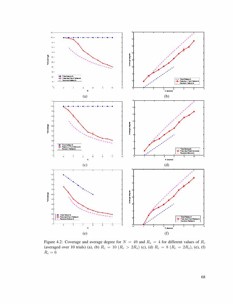
(a) (b)
(c) (d)
(e) (f)
Figure 4.2: Coverage and average degree for N = 49 and Rs = 4 for different values of Rc(averaged over 10 trials) (a), (b) Rc = 10 (Rc > 2Rs) (c), (d) Rc = 8 (Rc = 2Rs), (e), (f)Rc = 6
68

Figure 4.3: Variation of coverage with network size (N) for Rs = 4 and Rc = 8 (averaged over10 trials)
(a) θ = 2π3 (b) θ = π
2 (c) θ = 2π5
(d) θ = π3 (e) θ = 2π
7 (f) θ = π4
Figure 4.4: Sample deployments with 100 robots and Rc = Rs = 8.0.
69

(a) θ = 2π3 (b) θ = 2π
5 (c) θ = π3
Figure 4.5: Sample deployments in the presence of obstacles with 100 robots andRc = Rs = 8.0.
(a) (b)
(c) (d)
Figure 4.6: Performance of the Distributed deployment Algorithms for a deployment of 100robots in terms of (a) Coverage, (b) Edge Connectivity (c) Average Degree and (d) NET conditionsatisfaction
70

(a) (b) (c)
(d) (e) (f)
Figure 4.7: For θ ≤ 2π3 , the communication graph is a supergraph of RNG. (a) Communication
Graph (b) RNG (c) Difference for θ = 2π3 . (d) Communication Graph (e) RNG (f) Difference for
θ = 2π4
71

Chapter 5
Connectivity Maintenance and Coalescence
Communication connectivity is both essential and challenging for robot networks. While on
one hand robot groups rely on network-wide connectivity for coordination, on the other hand
maintaining connectivity in a large group of moving robots is hard because it imposes constraints
on robot motion. Another difficulty is that the communication range for most low power radios
is highly irregular [Zhao and Govindan, 2003] which adds to the unpredictability of connectivity.
Given the high cost of maintaining connectivity, we are interested in the question - what happens
if connectivity is lost? This situation could arise due to several reasons - robots could start in a
disconnected state, or accidentally lose connectivity due to failures, or intentionally disconnect
for efficient task completion. The cost of regaining connectivity, in terms of time and energy
spent, should be taken into account while designing the motion coordination algorithm. If the
cost is high the coordination algorithm should minimize the chances of disconnections and if the
cost is low it should allow the robots to occasionally disconnect and rejoin the network after task
completion.
72

Coalescence is the problem of isolated mobile robots independently searching for peers with
the goal of forming a single connected network. In this chapter, we study the time taken for
coalescence. We consider the scenario where the robots are memoryless (do not build a map)
and do not have any knowledge of the environment or positions of the other robots. Each robot
performs an independent random search and when two robots meet, they coalesce into a cluster
and the cluster thereafter sticks together and moves as a single random walk. This is illustrated in
figure 5.1. While the memoryless model is realistic for large swarms of simple robots, in several
applications robots will be capable of performing systematic exploration and mapping to speed up
coalescence. The coalescence time in this case is tied to the exploration algorithm and structure
of the domain and the memoryless random walk provides a simplified worst case study.
While coalescence can be considered a variation of the rendezvous problem, we use the term
coalescence to emphasize that the communication spread of the clusters increases as more robots
join. As we will show in section 5.2.3, the communication spread plays an important role in
determining latency. The basic idea is that robots need not be collocated to remain connected. If
they remain spread out, the disconnected robots will have a better chance of discovering them.
The coalescence time can be further improved if the clusters form an optimal shape such as
a line and move in a direction that maximizes the sweep area. This will involve a significant
coordination overhead because maintaining a formation while moving through an environment
with obstacles is challenging [Muhammad and Egerstedt, 2004]. Therefore we do not make any
assumption on the shape of the cluster.
The outline of the chapter is as follows. Section 5.1 presents the problem formulation and
mobility model. In section 5.2 we derive the coalescence time based on the meeting time of the
73

(a) t = 0 (b) t = MT 51 (c) MT 5
2
(d) t = MT 52 < t < MT 5
3 (e) t = MT 53 (f) t = MT 5
4 = CT (N = 5)
Figure 5.1: Illustration of Coalescence for N = 5. The dark red circles represent robots andthe yellow discs around them are their communication regions. The arrows show the randomwalk steps with the faded discs being the robot positions at the previous time instant. As robotscoalesce, the communication spread of clusters grows and the robots that are still searching havea better chance of hitting it.
mobility model. The coalescence time has an exponential distribution which is a function of the
number of robots, speed, communication range, and size of the domain. The main challenge
in the analysis is that the time between two clusters hitting each other depends on the size and
shape of the clusters which are both random and difficult to model. We make several simplifying
assumptions to make the analysis tractable which are validated using simulations in section 5.3.
We are particularly interested in the asymptotic behavior of the coalescence time with respect to
the size of the network, N . In section 5.2.3 we consider three extreme scenarios and show that
coalescence time is O( 1√N
) and Ω( log(N)N ). Simulations in MATLAB (section 5.3) verify these
bounds and also suggest that the lower bound is tight i.e. the coalescence time is Θ(log(N)/N).
74

(a) t = 0 (b) t = 1 (c) t = 7 (d) HT = t = 11
Figure 5.2: Illustration of random direction mobility model, RM . The blue cone and dark redcircle are a stationary node and the isolated robot respectively along with their communicationdiscs. The light yellow region is the area that the robot has “covered” in its search for the station-ary node.
5.1 Problem Formulation
We are interested in the following problem.
Given N isolated mobile robots placed at unknown locations within a bounded domain
D ⊂ <2, how long will it take for them to coalesce into a single connected component?
The goal of coalescence is to reach a state where all robots can communicate with each other
either directly or via other robots. Clearly, coalescence time will be depend on the communication
and mobility models of the robots. We use the following models.
5.1.1 Communication Model
All robots have a uniform binary disk communication with range R i.e. two robots can commu-
nicate with each other if and only if the distance between them is less than R. We say that two
robots “encounter” or “hit” each other when they are within communication range R and at some
75

time t ≥ 0 the area that a robot has “covered” is the union of the area that has been within its
communication range at 0 ≤ t′ ≤ t (figure 5.2).
5.1.2 Mobility Model
Each robot performs an independent random search for other robots. The motion strategy is a
simplified version of the Random Direction model [Aldous and Fill]. It is defined as follows
(figure 5.2). At each time step the robot
1. chooses a direction θ uniformly in [0, 2π)
2. moves in direction θ with a constant speed v for a constant distance l.
The random direction model results in a uniform stationary distribution.
At any point of time if two robots meet, they form a single cluster i.e. stay connected to each
other and move together following the same path. Similarly when two clusters meet they coalesce
to form a single cluster. Note that this interaction model does not affect the uniform stationary
distribution of the clusters.
5.1.3 Domain Model
For ease of analysis we assume that the domain is a torus. A more realistic boundary condition is
the reflecting model where the robots bounce back on hitting a boundary. However, it is known
that both the torus boundary condition and reflecting boundary condition retain the stationary
distribution of robots [Bettstetter, 2001]. Since stationary distribution is the only condition we
require of the torus boundary condition our analysis is valid for the reflecting boundary condition.
76

5.2 Coalescence Time Analysis
Coalescence time (CT ) is related to the time elapsed between robots meeting each other. There-
fore to model coalescence time, we must first understand the statistics of encounter times between
robots, called hitting time (HT ) and meeting time (MT ).
Definition 5.2.1 The hitting time of a mobility model is the time until a robot following the
mobility model encounters a static robot. If robot i moves according to the mobility model and
robot j is static, HT = mintt : ‖Xi(t)−Xj‖ ≤ R.
Definition 5.2.2 The meeting time is the time until two robots following the same mobility
model meet. If j also follows the mobility model described above and starts from its station-
ary distribution, the meeting time between i and j is the time before their first encounter.
MT = mintt : ‖Xi(t)−Xj(t)‖ ≤ R
We will now derive the hitting time and meeting time for our mobility model.
5.2.1 Hitting Time
Let robot i move according to the random mobility model and let α(t) represent the fraction of
domain area covered by the communication disk of i from time 0 to t. We can assume that this
area is uniformly distributed in the domain. Then the new area covered in the (t+ 1)th time step
is proportional to the fraction of uncovered area in D and is given by
α(t+ 1)− α(t) ≈ (1− α(t))2R`A(D)
(5.1)
77

where A(D) is the area of the domain. Solving the recursion, we get
α(t) ≈ 1−(
1− 2R`A(D)
)t(5.2)
If j is a stationary robot placed at a random position chosen uniformly in the domain, the
probability of hitting j at time t is equal to the fraction of the domain area covered by i, α(t).
Therefore the hitting time has the same exponential distribution as α(t) with mean
E[HT ] =A(D)2R`
(5.3)
Note that as expected, the hitting time is a function of the area of the domain, communication
range, and speed (step length).
5.2.2 Meeting Time
If both i and j start at a random positions chosen uniformly in the domain and follow the random
mobility model, then the meeting time will follow the same exponential distribution as the hit-
ting time with mean E[MT ] = E[HT ]/v [Spyropoulos et al., 2006] where v is the normalized
relative speed given by
v =‖~vi − ~vj‖
v(5.4)
If θ is the angle between the velocity vectors of i and j, then v can be computed as
12π
∫ 2π
0
√(1 + cosθ)2 + sin2θ dθ = 1.27 (5.5)
78

Figure 5.3: Verification of analytical model for kth meeting time, MTNk derived in equation (9)for N = 100, l = 100, and R = 20 averaged over 100 runs
For N = 2, the coalescence time CT is the meeting time. E[CT (n = 2)] = E[MT ] =
E[HT ]/1.27.
5.2.3 Coalescence Time
Let MTN1 ≤ MTN2 ≤ · · · ≤ MTNk ≤ · · · ≤ MTNN−1 be the 1st, 2nd, · · · , kth, · · · (N − 1)th
meeting times in a network of size N . The coalescence time CT (n = N) = MTNN−1.
We will now find an expression for the kth meeting time MTNk . The first hitting time is
the minimum of(N2
)meeting times between the different pairs of robots. Since each of these is
independent and has an exponential distribution,
79

E[MTN1 ] =1(N2
) · E[MT ] =2
N(N − 1)· 1
1.27· A(D)
2R`(5.6)
t = MTN1 , there areN−1 clusters with 1 cluster consisting of two robots andN−2 clusters
consisting of 1 robot each. At t = MTNk , there are N − k clusters in the domain. The number
of robots in each cluster is a random variable. At t = MTNk+1 two of these N − k clusters
meet and coalesce to form a bigger cluster. We expect that the time elapsed between clusters
meeting will also have an exponential distribution similar to the first meeting time MTN1 . The
challenge is that this meeting time will depend on the size and shape of the clusters which is
difficult to estimate. Even if we know the number of robots in each cluster, the shape will still
be random. We will make a simplifying assumption that all clusters have the same size. Further,
we assume that the expected shape of the cluster is a disc since clusters coalesce in all directions
with equal probability. We validate these assumptions using simulations in MATLAB described
in section 5.3. The meeting time derived based on these assumptions is surprising close to the
simulation results (figure 5.3). Based on equation (6) we write the following
∆MTNk+1 = MTNk+1 −MTNk
E[∆MTNk+1] =2
(N − k)(N − k − 1)· 1
1.27· A(D)
2Reff `(5.7)
where Reff is the effective radius of the clusters. Reff depends not only on the size of the
clusters but also the shapes. At t = MTNk , there are N −k clusters. If we assume that the area of
a cluster grows linearly with the number of robots the the total area of all clusters at t = MTNk
80

is NπR2 − kβπR2. Therefore the area of each cluster C at t = MTNk is A[Ck] = πR2(N−kβN−k )
where 0 ≤ β < 1 is a constant. For the optimal case when robots are at a distance from R of
each other, β ≈ 0.2. Approximating the shape of each cluster as a disc, we get Reff =√
N−kβN−k .
Substituting in the above equations we have
E[∆MTNk+1] ≈ 2(N − k)(N − k − 1)
· E[MT ]√(N−kβN−k )
(5.8)
E[MTNk ] =k−1∑
0
E[∆MTNk+1]
=k−1∑
0
2(N − k − 1) · (N − k)
E[MT ]√(N−kβN−k )
(5.9)
We now have an expression for coalescence time in terms of the number of robots, N and the
expected meeting time E[MT ] which in turn is a function of size of the domain D, communica-
tion range, R, and step length or speed `.
E[CT (n = N)] = E[MTNN−1] =N−2∑
0
E[∆MTNk+1]
=N−2∑
0
2(N − k − 1) · (N − k)
E[MT ]√(N−kβN−k )
(5.10)
The asymptotic behavior of the coalescence time as the number of robots N increases is
not clear from the above expression. Therefore we will consider three cases where the analysis
is tractable. In the first case, we will assume that the communication area of clusters does not
81

Figure 5.4: The mean Coalescence Time is bounded by O( 1√N
) and Ω( log(N)N ). The graph shows
the coalescence time(CT ) as a function of network size(N ) averaged over 200 runs with l = 100and R = 20 on a linear scale.
change when robots join i.e. every cluster is a disk of πR2 irrespective of the number robots it
contains. As expected this case gives a very loose upper bound on the coalescence time. Second,
we will assume that there is only one cluster that robots coalesce to upon hitting and ignore
interactions between all other clusters. This case is equivalent to the stationary base station case
and gives us a O( 1√N
) upper bound. Lastly, we will derive a lower bound using an idealized case
where the number of clusters decreases exponentially with time i.e. at each meeting time, every
cluster coalesces with exactly one other cluster.
82

Figure 5.5: The mean Coalescence Time is bounded by O( 1√N
) and Ω( log(N)N ). The graph shows
the coalescence time(CT ) as a function of network size(N ) averaged over 200 runs with l = 100and R = 20 on a log scale.
Case 1: Ignoring area growth
At t = MTNk there are N − k clusters each of which has a disc shape of radius R. Substituting
Reff ≥ R in equation (8) we get
83

E[∆MTNk+1] ≤ 2(N − k)(N − k − 1)
· E[MT ]
E[MTNN−1] =N−2∑
0
E[∆MTNk+1]
≤N−2∑
0
2(N − k − 1) · (N − k)
· E[MT ]
=N−2∑
0
2(1
N − k − 1− 1N − k
) · E[MT ]
= 2(log(2)− log(N) + log(N − k + 1)) · E[MT ] (5.11)
We get, E[CT (n = N)] = E[MTNN−1] ≤ log(2) ·MT i.e. the coalescence time is at most
a constant times the meeting time irrespective of the size of the network. As we will see in
the simulation results, this is a very loose bound for the coalescence time which means that the
communication area growth plays an important role in decreasing the coalescence time.
Case 2: Single cluster
Suppose there is one special robot in the network that robots coalesce with upon meeting. En-
counters between all other clusters do not affect the random motion of robots and in particular, do
not result in robots coalescing. This simplifies analysis because the number of robots in different
clusters is no longer random. At time t = MTNk , there is 1 cluster consisting of k+ 1 robots and
N − k − 1 single-robot clusters. Again, we assume that the area of a cluster grows linearly with
the number of robots. At t = MTNk , the cluster Ck contains k robots and A[Ck] = πR2(1 + βk)
84

where 0 < β ≤ 1 is a constant. Since robots can join the cluster in all directions with equal prob-
ability, we approximate the shape of the cluster as a disk. This give us Reff =√
1 + β · k · R.
At t = MTNk , each of the N − k − 1 isolated robots are uniformly distributed and have an
equal chance of meeting the cluster. Therefore the time before the MTNk+1 is the minimum of the
N − k − 1 meeting times.
E[∆MTNk+1] ≤ 1(N − k − 1)
· E[MT ]√1 + β · k
E[MTNN−1] =N−2∑
0
E[∆MTNk+1]
≤N−2∑
0
1(N − k − 1)
1√1 + β · k
· E[MT ]
≈∫ N−1
0
(1
(N − x− 1)1√
1 + β · x· E[MT ]
)dx
=
2 · tanh−1(√βx+1√
Nβ−β+1)
√Nβ − β + 1
N−1
0
= Ω(
1√N
)(5.12)
85
Case 3: Simultaneous meeting
We will now derive a lower bound on coalescence time by considering an extreme scenario where
at each meeting time, every cluster simultaneously hits one other cluster. Let N = 2p.
E[∆MTNk+1] =1(
2p−k
2
) 12k· E[MT ]
=1
2p−k · (2p−k − 1)1
2k−1· E[MT ]
E[MTNN−1] =p−1∑
0
12p−k · (2p−k − 1)
12k−1
· E[MT ]
= 2−p · p · (log(2)− 1) · E[MT ]
= Θ(
log(N)N
)(5.13)
In the next section we will verify these bounds through simulations.
5.3 Simulation Results
Simulations were conducted in MATLAB to verify the analysis. The domain used is a 2D torus.
The parameters to the program are number of robots N , step size `, communication rage R and
torus side T . The robots start at random positions uniformly distributed over the torus. Every
robot picks a random direction and moves with a uniform speed of 1 unit per time step. At each
time step, the robot checks if it is within a distance R of another robot, in which case, the robots
coalesce and follow the motion of the robot with the smallest ID. After ` time steps, each cluster
picks a new direction. The simulation stops when there is only one cluster.
86

We first verify the model for meeting time (equation (9)). This expression was was based
on three simplifying assumptions 1) the clusters sizes are close to uniform, 2) the shape of the
clusters is close to circular and 3) the area of a cluster grows linearly with the number of nodes.
The results from simulation plotted in figure 5.3 are very close to the analytical expression and
validate our model.
Our next set of experiments simulated Coalescence and measured Coalescence Time as a
function of N . Figure 5.4 compares the mean Coalescence Time to the analytical expressions
derived above. Our objective is to compare the shapes of the curves and the constants in the
expression were found empirically. We see that the coalescence time has bounds of O( 1√N
) and
Ω( log(N)N ).
5.4 Conclusions
We consider the problem of coalescence, i.e. isolated robots independently searching for peers
and forming a single connected component. Coalescence strategies can complement algorithms
for robot collaboration that require a connected network. In the absence of localization or any
information about the environment, the robots can perform a simple random walk search till they
are within the communication range of other robots. We show using probabilistic analysis that
for such a strategy, Coalescence Time has an exponential distribution which is a function of the
number of robots, speed, communication range, and size of the domain. Further, it decreases as
O( 1√N
) and Ω( log(N)N ) with the number of robots, N . Even though the analysis is approximate,
there is a surprisingly good match with the simulation results.
87

Chapter 6
Coverage Optimization in Complex Environments
In this chapter, we address the coverage problem for mobile sensors with location dependent
sensing models. In reality, the performance of each sensor is impacted by the environmental
conditions in which the sensor is located. We observed this while exploring the possibility of
deploying a camera sensor network involving cyclops image sensors [Rahimi et al., 2005] to
monitor indoor and outdoor pathways. We conducted the following simple experiment. Figure
6.2(a) shows an aerial view of a botanical garden. We placed 11 cyclops image sensors(Figure
6.2(b)) uniformly along a path in the garden as shown in Figure 6.3(a). We used the standard
background-subtraction-based detection algorithm in [Horprasert et al., 2000] to test the number
of times a person walking along the path was detected by this network. The results are shown in
Figure 6.3(c). We repeated the same experiment for an alternate sensor arrangement as shown in
Figure 6.3(b) – this time used sensing performance data from various locations along the path.
The detection results in this case were far superior (Figure 6.3(d)).This is due to the fact that
background subtraction is sensitive to lighting conditions that vary from location to location in
the deployment domain. As a result the sensing performance of the image sensors varies from
88

(a) (b)
Figure 6.1: (a) An aerial view of the garden (b) the pathway to be covered
Figure 6.2: Cyclops camera with an attached Mica2 Mote
location to location. In a recent work in [Shi et al., 2007], the authors report that underwater
sound propagation is susceptible to changes in water salinity and temperature and therefore the
listening range, or coverage, of a sound detector is largely influenced by its location underwater.
Currently, coverage algorithms do not address such location dependence. This leads to inefficient
usage of resources.
89

(a) (b)
(c) (d)
Figure 6.3: Node locations for (a) uniform deployment and (b) optimized locations and theirdetection results. The graphs illustrate detection events by node numbers (y-axis) at a given timestep (x-axis). The red squares indicate false-positives.The optimized placements use 9 nodeswhile uniform placements use 11 nodes
For this variation of the coverage problem, we develop a distributed control algorithm based
on the generalized Voronoi partitioning to obtain optimal sensor arrangements with guaranteed
convergence. Cyclops camera sensors provide a wonderful playground to apply our algorithms.
We consider the problem of covering indoor and outdoor pathways with Cyclops camera sen-
sors. Cheap and low-power imaging sensors such as Cyclops and CMUCam [Rowe et al., 2002]
along with Motes have been demonstrated to have many potential applications in monitoring and
surveillance. Because of the constraints on memory, computation and energy resources available
to the imagers, they will most likely use simple image processing such as background subtraction
for object detection. It is is well known that background subtraction is sensitive to changes in the
background and lighting conditions making the sensing performance location-dependent.
90

Our contributions
We formulate the coverage problem as the locational optimization problem with the sensing per-
formance function that is location dependent, i.e., it is a function of the distance between the
sensor and the sampling location as well as the location of the sensor. In the same spirit of the
coverage algorithms in [Cortes et al., 2004], we propose a distributed control and coordination
algorithm for the new formulation. The convergence of the algorithm is proved. We apply these
ideas to the problem of covering indoor and outdoor pathways using Cyclops cameras. Based on
several indoor and outdoor measurements we propose a 1D empirical function for the sensing
performance for the Cyclops sensor. The sensing performance function corresponds to the num-
ber of pixels detected of the test object at different locations based on the standard background-
subtraction-based algorithm [Horprasert et al., 2000]. The function is characterized by two pa-
rameters that vary with the location of the camera sensor thus capturing the location dependence
of the sensing performance. Based on this, we formulate the problem of covering pathways as
a 1D coverage algorithm. We present simulation results for various forms of the functions for
the parameters and demonstrate convergence of our algorithm. In reality, these functions are not
known a priori. Using the history of measurements as camera locations evolve, we estimate the
functions using a piecewise linear form. We present simulation results using this approach. We
conducted experiments in indoor setting under controlled lighting as well as in outdoor settings at
fine scales to find values of the parameters in the performance functions. We present simulation
results on this physical data and demonstrate the performance of our algorithm.
The rest of the chapter is organized as follows. In Section 6.1 we formulate the coverage
with problem with the location dependent sensing performance function. A distributed control
91

algorithm is proposed in Section 6.2 and its convergence is proved. In Section 6.3, we study ap-
plication of the control algorithm to the problem of covering indoor and outdoor pathways using
cyclops cameras. We propose a sensing performance function of the cyclops camera capturing
the location dependence and present simulation and experimental results.
6.1 Problem Formulation
We build on the notation used in [Cortes et al., 2004] to define our coverage problem. Let Q
denote the bounded convex domain in R. We seek to cover Q using n mobile sensors. Let
φ : Q→ R denote the scalar density function. It captures the importance of covering a particular
location. Let p1, p2, · · · , pn denote the current locations of n sensors. We assume a location-
dependent sensing model for each sensor, i.e., the sensing performance at point q for the ith
sensor not only depend on ||q − pi|| but also on the location, pi itself. Here, || · || denotes
the Euclidean norm. We denote the sensing performance function for sensor i at point q by
f(||q − pi||, pi), where f : R+ × Q → R. Note that we explicitly indicate the dependence of
the performance function on the sensor location. The performance function naturally induces a
generalized Voronoi partition of Q. Each sensor has its own dominance region, i.e., its Voronoi
cell where the sensing performance is better than that for any other sensor. More formally, if Wi
denotes the dominance region for the ith sensor, then
Wi = q ∈ Q | f(||q − pi||, pi) ≥ f(||q − pj ||, pj), ∀j 6=i. (6.1)
92

Now we define our coverage metric or net utility function as follows:
H(p1, p2, · · · , pn) =n∑i=1
∫Wi
φ(q)f(||q − pi||, pi)dq (6.2)
The utility function is the sum of the sensing performance function of each sensor over its
dominance region including the weighing density function. We refer to∫Wiφ(q)f(||q−pi||, pi)dq
as the utility of the ith sensor. We formulate the coverage problem as finding the optimal set of
locations of the sensors that maximizes the net utility.
arg maxH(p1, p2, · · · , pn) (6.3)
Note that it is possible to formulate other metrics such as maximizing the minimum over
the utility functions of all the sensors, as suggested in the literature, e.g., [Cortes et al., 2004].
We would like to note that in the common literature [Cortes et al., 2004] the coverage objective
function is known as the locational optimization function and the coverage problem is formulated
as the minimization problem. In the spirit of the application we consider in this chapter, we
formulate the problem as the maximization problem.
6.1.1 Partial derivative of the overall utility function
We note that the result about the partial derivative of the net utility function based on the diver-
gence theorem [Cortes et al., 2004] generalizes easily to our case.
93

Lemma 6.1.1 The partial derivative of the net utility function with respect to the position of the
i-th sensor is given by,
∂H∂pi
=∫Wi
φ(q)∂f(||q − pi||, pi)
∂pidq (6.4)
We refer readers to [Cortes et al., 2004] for the proof of the lemma.
6.2 Distributed coverage control
We propose a distributed coverage control algorithm that is based on iterative local sub-gradient
method.
6.2.1 Control Law for each sensor
Let pi(n) be the position of the i-th sensor after n updates. We state the control law for the
position update of the i-th sensor to pi(n+1). During the time the i-th sensor updates its position
from, our coverage algorithm does not allow the simultaneous update at the Voronoi neighbors
of the i-th sensor. The local control law involves searching for the local optimal solution. Given
that the positions of the Voronoi neighbors are fixed, the net utility H and the local gradient, ∂H∂pi
are just the functions of pi. We state the control law as follows.
pi(n+ 1) = p∗i ,where, p∗i = arg maxpi∈Wi
H(· · · , pi, · · · ) (6.5)
Essentially, the control law involves local search over the Voronoi partitionWi for the optimal
solution p∗i by solving the constrained optimization problem. If p∗i does not lie on the boundary
of Wi, then it is the root of equation g(pi) = 0. Since the search involves finding the optimal
94

location just for one sensor, it is computationally tractable. We state the following lemma about
the increase in the net utility after every pose update.
Lemma 6.2.1 The control law for an individual sensor in Equation 6.5 guarantees that the net
utility increases after the position update of the sensor.
Implementation of the above control law requires the exact knowledge of the sensing perfor-
mance function f(||q − pi||, pi) for each sensor i and the density function φ(q). Later we show
in our case study of camera sensor network that f(||q− pi||, pi) can be estimated on the fly using
measurements. We also note that in [Schwager et al., 2007] it is shown that the global knowledge
of φ(q) is not required.
6.2.2 Distributed Coverage Algorithm
Below we state the coverage algorithm that runs at each node. We assume discrete time steps, 1,
2, · · · . The algorithm involves the implementation of the local control law that we described in
the previous section. A node updates its position only if its Voronoi neighbors are not updating
their positions.
t : Update Vit+1: Check if any j ∈ Vi is updating its positiont+2: if yes, wait for random duration of time and repeat the above stepst+2: if no, schedule position update at t+3 and broadcast over Vit+3: start moving to optimal p∗i as obtained using Equation 6.5t+k: After the move, wait for random duration before the next update
Algorithm 1: Coverage algorithm at the i-th sensor: Let pi denote its position. Let Videnote the set of its Voronoi neighbors.
95

6.2.3 Convergence
Theorem 6.2.2 The distributed coverage algorithm at each sensor as described in Algorithm 1
converges, as the number of position updates tends to infinity.
The proof follows from the fact that the net coverage utility is bounded and by lemma 6.2.1,
it increases monotonically with each iteration of the algorithm.
The algorithm yields a local optimal solution to the coverage problem. Comments about the
optimal solution.
6.3 Deployment of Cyclops camera networks
In this section, we discuss implementation issues and results of our algorithm for the coverage
problem using Cyclops camera sensors.1 The Cyclops camera sensor consists of a CMOS im-
ager with CIF image capability and an internal image processor unit for image interpretation and
analysis. It couples with a Mote and periodically captures images (figure 6.2). Our objective is to
cover loopy environments such as indoor corridors or outdoor pathways such that an intruder ob-
ject can be detected. We show that this problem can be mapped into a suitable coverage problem.
We first propose a model for the sensing performance function of a camera.
6.3.1 Sensing Performance Function
Our choice of the sensing performance function of a camera is related the performance of the
object detection algorithm that is based on background subtraction. Foreground object detection
using background subtraction has been used extensively in video surveillance applications due1We do not consider any network related issues here.
96

to ease of implementation and effectiveness [ref]. This method has low resource requirements
in terms of memory and computation and is therefore well suited for low complexity camera
sensor networks. According to this method, the cyclops camera periodically captures images and
maintains a moving average background model of the environment. A foreground model is also
constructed as the absolute difference of the instantaneous image and the constructed background.
The resulting foreground images are then are passed through a luminance and size filter, which
identifies clusters of pixels that have a considerable change in illumination. See [ref] for the
details of the algorithm. Figure 6.5(a) shows a cyclops camera set up in a corridor in a building.
Figure 6.5(b) and 6.5(c) show the background model and the instantaneous image obtained by
placing a white board at some distance. The foreground images as the difference between the
two images is shown in Figure 6.5(d). The detectability of the object depends on the number
of pixels identified after passing the foreground model through the filter – larger the number of
pixels, better the detection probability. We therefore use the number of pixels identified as the
sensing performance function for each camera sensor. Note that the number of pixels detected is
also a function of distance between the camera and the object. The further away the object is, the
lower the number of pixels detected will be.
Suppose a rectangular object of dimension h × w placed at a distance d on the camera’s
central axis exactly facing the camera. Consider an ideal scenario in which every point on the
object differs significantly in its illumination characteristics from the background image. Then,
97

Figure 6.4: Perspective projection model
(a) (b) (c)
Figure 6.5: Illustration of pixels on target not detected. (a) background image (b) original imageand (c) foreground image. In the foreground image, some of the pixels in the target board areblack. These are the pixels that are similar to the background and are therefore not detected bythe camera.
98

according to a perspective projection camera model, the number of pixels, m, detected by the
camera is approximately given by:
m ' f · h · wd2
· resolutionsensor area
= k · h · wd2· resolution
where f is the focal length and k is a constant. Figure 6.4 shows the perspective projection model.
Thus, the number of pixels detected is inversely proportional to square of the distance between the
camera and the object. We indeed observed this relationship in practice when we experimented
with a white board of dimension 3ft × 2ft placed at different distances in front of a cyclops
camera that was placed in a well-lit corridor. Figure 6.6.1(a) shows the experimental set-up and
Figure 6.6.2(a) shows the number of pixels identified using the background subtraction algorithm
as a function of distance between the camera and the white board. We indeed observe the trend
that the number of pixels are inversely proportional to the squared distance. However these
situations are rare in the environments where the lighting conditions and the object properties are
far from the ideal situation. In practice, the number of pixels detected by the camera deviates from
this ideal model because some pixels on the object have the same texture as that of the background
and go undetected. This is illustrated in fig 6.5 where the target is a white rectangular board. In
the foreground image, the pixels in white are the ones that are detected. Some of the pixels on
the board have intensities close to their corresponding pixels in the background.
This indicates that the sensing performance function of camera depends not only on the dis-
tance but also on the location of the camera itself. This very behavior motivates the definition
99

of the coverage problem we address. We restrict ourselves to coverage of narrow pathways re-
ducing the problem to coverage of 1D loops. We conducted a series of experiments both indoors
and outdoors to extract the sensing performance function of a camera. We placed a white/black
rectangular board in front of a camera along its central axis at increments of 5 feet to obtain the
number of pixels detected. Based on several data sets we observed that the following empirical
model for the sensing performance function best fits the data.
f(||x− q||, x) =k1(x)
k2(x) + ||x− q||2(6.6)
Here x denotes the location of the camera and q denote the sensing performance, i.e., the
number of pixels detected at location q. Note the dependence on the location of x via functions
k1(x) and k2(x). Figure 6.6 shows the best fit and the corresponding values of k1 and k2 for
indoor and an outdoor instances. Note that the sensing performance function is not exact; it
corresponds to the best fit with the data.
6.3.2 Coverage Algorithm for 1D loop
In this section, we discuss the coverage problem formulation and algorithm for covering a loopy
pathway using the cyclops cameras. We assume that the pathway is narrow enough so that we
formulate the problem as a 1D coverage problem. We assume that each sensor is a bi-directional
camera obtained by combining two cyclops camera modules aligned along the same axis. Thus
each sensor can see on its left and right directions on the loop. The sensing performance function
along each direction takes the form of Equation 6.6 with possibly different parameter values.
For now we assume that the pathway is a smooth curve that can be parametrized with a single
100

1(a) 1(b) 1(c)
2(a) 2(b) 2(c)
Figure 6.6: Validation of the proposed model for pixels detected vs. distance for three differentenvironments. 1(a) is a well-lit corridor and close to an ideal environment. 2(a) is an outdoorpathway with shadows of trees and buildings. 3(a) is inside a lab where the lighting conditionsare not uniform. The solid blue line is the number of pixels detected from experiments and thered dashed line is the minimum least squares fit using the model in Equation 6.6
101

parameter and does not contain any sharp corners, i.e., at any location the curvature of the loop
is very large compared with the local detection range of the camera assuming that the sensor is
always aligned on the loop such that its central axis is always tangential to the loop. Let n be the
number of cameras and let p1, p2, · · · , pn denote their locations on the loop in the order such that
pi is between pi−1 and pi+1. Further, let pn+1 = p1. Let fl(||pi − q||, pi) and fr(||pi − q||, pi) be
the left and the right sensing performance functions respectively of the i-th camera located at pi.
We assume that both fl and fr have the empirical form described in Equation 6.6:
fl(||pi − q||, pi) =k1l(pi)
k2l(pi) + ||pi − q||2(6.7)
fr(||pi − q||, pi) =k1r(pi)
k2r(pi) + ||pi − q||2(6.8)
Because the problem is 1D, the region of dominance of any sensor corresponds to a segment
on the loop. We further assume that the region of dominance of the i-sensor strictly belongs to the
interval (pi−1, pi+1). In other words, there are no abrupt changes in the sensing behavior over the
domain such that each sensor contributes to the net utility function. Let [li, ri] be the dominance
range of the i-th sensor. Thus, li ∈ (pi−1, pi) and ri ∈ (pi, pi+1). According to the definition of
the dominance region,
fl(||pi − li||, pi) = fr(||pi−1 − li||, pi−1) and,
fr(||pi − ri||, pi) = fl(||pi+1 − ri||, pi+1).
102

Using the above notation, the net utility function in 6.2 assuming uniform density function
(φ(q) = 1) can be expressed in the following form for the case of 1D loop.
H(p1, p2, · · · , pn) =n∑i=1
∫ pi
li
fl(||pi − q||, pi)dq +∫ ri
pi
fr(||pi − q||, pi) (6.9)
6.3.3 Simulation Results
Simulation Environment
We ran simulations in MATLAB to test the convergence and resulting coverage of our distributed
control law. The path is a 1D loop that can have sharp corners and obstacles that cause the sensing
performance function to vary abruptly. The sensors start at randomly chosen initial positions and
in each iteration of the algorithm, they update their position according to Equation 6.5 using a
constrained optimization routine in MATLAB. We assume that sensors are localized and adjacent
sensors on the path can communicate with each other. The simulation converges when the no
sensor changes its position. We test for different models of k1(x) and k2(x), different shapes of
the path, and different number of sensors.
Global knowledge of sensor performance function
We first consider the ideal scenario where sensors have perfect knowledge of the sensing perfor-
mance function. In practice, the sensors will estimate the performance function based on observed
data the performance of the coverage algorithm will depend on the accuracy of this estimation.
103

1(a) 1(b) 1(c)
2(a) 2(b) 2(c)
3(a) 3(b) 3(c)Utility
Figure 6.7: Performance of the distributed control law for three types of parameter functions ona 1D loop which is a 250 feet long smooth curve. 1(a), 2(a) and 3(a) show the parameter valuesconstant, sine and step. 1(b), 2(b) and 3(b) show the corresponding final positions of sensors (redcircles) superimposed on the k1 function. The crosses show the dominance region boundariesbetween sensors. 1(c), 2(c) and 3(c) show the variation in the net coverage utility. The utilityincreases monotonically with each iteration.
104

(a) (b)
Figure 6.8: Variation in coverage utility and convergence time for different network sizes aver-aged over 50 iterations.
1(a) 1(b) 1(c)
2(a) 2(b) 2(c)
Figure 6.9: Performance of the distributed control law in the presence of occlusions - (1) obstaclesand (2) sharp corners.
105

Figure 6.7 shows the performance of the algorithm for three different sensing performance func-
tions. In each case, the sensors start at random initial locations. As expected, for constant pa-
rameter values (Figure 6.7.1(a)), the sensors converge to a uniform distribution(Figure 6.7.1(b)).
When the parameters have significant variations (Figure 6.7.2(a), 6.7.3(a)), the distribution if
non-uniform (Figure 6.7.2(b), 6.7.3(b)). Sensors try to move to positions where the value of k1 is
large and k2 is small so that their local utility is maximized. Note that in each case the global cov-
erage utility increases monotonically even though the position updates at each sensor are local.
This is in agreement with Theorem 4.2. To study the impact of the network size on the algorithm
performance, varied the network size from 5 to 100. For each network size, we repeated the sim-
ulation 50 times starting with a different random initial position each time. The coverage utility
increases exponentially and eventually saturates (Figure 6.8(a)) since as the number of sensors
increases, the marginal utility of each additional sensor decreases and tends to zero. The varia-
tion in utility is very small indicating that the initial locations do not impact the final coverage.
The convergence time initially increases with the number of sensors and then stops increasing
(Figure 6.8(b)) proving that the algorithm is scalable. The large deviations indicate that unlike
coverage, the convergence time varies significantly with the initial sensor locations.
106

Occlusions
Occlusions can occur due to obstacles in the path or sharp corners. Since the camera cannot sense
beyond an occlusion, it cause an abrupt drop in the sensing performance function. Equations 6.7,
6.8 can be modified as follows to account for occlusions.
fl(||pi − q||, pi) =
k1l(pi)
k2l(pi)+||pi−q||2 if q is not occluded from pi
0, otherwise
(6.10)
fr(||pi − q||, pi) =
k1r(pi)
k2r(pi)+||pi−q||2 if q is not occluded from pi
0, otherwise
(6.11)
Because the sensing function takes on a constant value for points beyond an occlusion, it is
possible that the equations fl(||pi − li||, pi) = fr(||pi−1 − li||, pi−1) and, fr(||pi − ri||, pi) =
fl(||pi+1 − ri||, pi+1) that define the dominance region have many solutions. This will happen,
for example, when adjacent sensors have two or more obstacles between them. For such cases,
we define the dominance region boundary to be the position of its closest occlusion i.e., if the
value of the sensing function of a camera is zero at a point q then q is considered not covered
by the camera and will not belong to its dominance region. Notice that with this definition, the
dominance regions may not form a partition of the path and there could be segments of the path
that do not belong to any sensor’s dominance region. However, since these segments have zero
coverage utility for all the sensors, and the rest of the path is partitioned according to the Voronoi
107

property, this definition of dominance regions is an optimal assignment of points on the path to
sensors.
With these new definitions for performance function and dominance regions, we can apply
the control law in equation 6.5 and Theorem 4.2 guarantees convergence. However, with this
control law, sensors adjacent to occlusions will not cross the occlusions because they only pick
new positions within their dominance regions. To further improve the coverage utility, we intro-
duce an additional switching step where sensors can cross obstacles if the local utility gained by
doing so is more than the utility gain of the optimal location within its dominance region. While
computing the switching utility, we account for change in the dominance regions and the utility
of the neighboring sensors. Note that the local utility of every other sensor remains unchanged.
Figure 6.9.1 shows the result of the algorithm on a loop of length 250 feet with 3 obstacles.
The parameters vary as sine functions. Figure 6.9.1(b) shows the positions of the obstacles (black
squares) and final positions of the sensors (red circles). Figure 6.9.2 shows an example on a
rectangular path with 4 sharp corners that cause occlusions. In both cases, the utility increases
monotonically with each iteration and the algorithm converges. As expected the coverage ob-
tained here is less than Figure 6.7.2(a) where there are no occlusions. We can generalize this
approach to deal with more complex pathways with multiple junctions so at a sensor adjacent to
a junction reasons about the coverage gain in each of the branches that meet at the junction.
Online estimation of sensor performance function
In the coverage algorithm in the previous section we assumed that each sensor has global knowl-
edge of the sensing performance function f(||pi − q||, pi). This permits a sensor to take the best
108

(a) (b) (c)
Figure 6.10: Performance of the distributed control law with partial knowledge of k1(x) andk2(x).
step according to Equation 6.5. However in practice this is not possible. Specifically, in case of
camera sensors, functions k1(x) and k2(x) are not globally known. This necessitates modifica-
tion of the current coverage algorithm. We assume that at every step of the algorithm, a camera
learns its sensing performance function, i.e., the empirical values of k1 and k2.
In the simulations shown in Figure 6.10, each sensor builds piecewise linear models of k1
and k2 based on data from its neighboring sensors and its current data. To improve the estimation
in the first iteration, we assume that sensors share data over multiple hops. We observe that
the utility sometimes decreases because of erroneous estimation (Figure 6.10(c)). But even with
this very simple estimation, the coverage utility is close to the case when global knowledge was
assumed.
6.3.4 Cyclops Experiments and Results
We conducted a series of controlled experiments with cyclops cameras to gather several images
in two different environmental settings – indoor and outdoor. We used interpolation techniques
109

(a) indoor (b) outdoor
Figure 6.11: Cyclops setup
on the gathered data to reconstruct the sensing performance functions in these settings and tested
the performance of our coverage algorithm for these pseudo-real functions.
1) a rectangular corridor in an building with controlled lighting (figure 6.11(a)) a rectangular
pathway surrounded by trees with uncontrolled lighting (figure 6.11(b)). For each of these set-
tings, we picked sample positions for the camera and for each location, we estimated the sensing
performance function (k1 and k2) by placing a target at different distances from the camera.
Indoor experiments
Corridors of buildings provide an ideal playground for testing our coverage algorithms with cy-
clops cameras. We performed experiments under controlled lighting conditions in a rectangular
corridor of which the central axis rectangle is of size 90ft× 30ft. The corridor is 5ft wide and
Figure 6.11(a) shows a cyclops camera set up along the length of the corridor. At every 20ft
along the lengthwise central axis of the corridor, we placed a cyclops camera and captured on
110

both sides the images of the corridor which serve as background models. We also captured im-
ages of a white or black board of dimension 3ft× 2ft placed along the central line kept at every
5ft from the camera up to 25ft. These images serve as foreground models. Since the width of
the corridor is 30ft, along the widthwise central axis, we placed a camera at the middle point
and captured images on both sides in the similar fashion. We used these images to fit the sensing
performance function to obtain the values of k1 and k2 at various locations. Along the entire
corridor, we obtained 22 pairs of values of k1 and k2. We interpolate spline functions through
these values of k1 and k2 to estimate the pseudo-real global sensing performance function. Fig-
ure 6.12(a) shows k1(x) and k2(x) along the entire length of the corridor. We use this form to
test our coverage algorithm.
In our simulations, we placed k sensors initially uniformly randomly. simulations results -
comment about number of sensors, utility, global knowledge / vs online estimation, convergence
Outdoor experiments
We conducted a similar experiment as in indoor case around an outdoor rectangular pathway
surrounded by trees without any control over lighting conditions. The pathway was of size a× b
and Figure 6.11(b) shows a picture of a cyclops camera set up along the pathway. We captured
background images and foreground images at n locations around the pathway in both directions.
We observed that the lighting conditions in the outdoor setting change rapidly and because of
this effect we collected data at relatively a few spots. Based on these images, we estimated the
values of k1 and k2 at the sampling points. We interpolate spline functions through these values
111

(a) (b)
(c) (d)
Figure 6.12: Performance of the distributed control law in an indoor rectangular corridor. (a)Sensor model parameters for left facing camera, (b) Sensor model parameters for right facingcamera, (c) final locations (d) utility
112

(a) (b)
(c) (d)
Figure 6.13: Performance of the distributed control law in an outdoor environment. (a) Sensormodel parameters for left facing camera, (b) Sensor model parameters for right facing camera,(c) final locations (d) utility
113

to obtain the sensing performance function over the domain and Figure 6.13(a) shows this model.
We use this model to test our coverage algorithm.
Dynamic Environments
All the experiments we conducted involved manual positioning of the cameras and the test boards
and was very time consuming. Unlike the indoor environments, the lighting conditions in outdoor
environments change rapidly relative the time scale of collecting all the measurements. However
we believe that with some degree of automation, our coverage algorithm can easily implemented
in dynamic environments that demand frequent reconfiguration of the sensor positions. In partic-
ular, we imagine that the cyclops cameras and the testing board be mounted on mobile platforms
that will have localization ability. The images can be processed on board to estimate the sensing
performance function at the current location. By means of wireless communication the sensors
can implement distributed coverage algorithm. We restricted our work to a simple pixel detection
algorithm. It is possible to implement other kinds of algorithms to improve the local sensing
performance functions. But our coverage algorithm still holds in this scenario.
6.4 Conclusions
We addressed the coverage problem where the performance of each sensor depends on its loca-
tion. We formulate the coverage problem as a locational optimization problem and propose a
distributed algorithm with guaranteed convergence. We applied our algorithm to the problem of
covering indoor and outdoor pathways using Cyclops camera networks. Based on several mea-
surements we proposed an empirical function for the sensing performance of the Cyclops camera.
114

We presented simulation results for various scenarios and demonstrated that our algorithm con-
verges. We also presented simulation results on the data collected at fine scales in indoor and
outdoor settings. As a part of future work we planning to apply our algorithm in 2D situations.
115

Chapter 7
Conclusions and Future Work
The central thesis of this work is that “Mobility can be effectively used for topology control of
robot networks. In the following we summarize the key contributions and discuss directions for
future work.
1. Network Geometry: Local conditions that affect global topological properties aid scala-
bility and can drastically reduce the complexity of robot controllers. Recently, it has been shown
that for a disk graph in a two-dimensional plane, if each node has one neighbor in every θ < π
sector then the network is guaranteed to be 1-connected [Xue and Kumar, 2006]. We extended
this result to show that θ < 2πk < π guarantees k-edge-connectivity. Surprisingly, the condition
for k-connectivity applies to any general (non-disk) graph in a two-dimensional plane provided
the graph is 1-connected. This implies that the condition only depends on the angles between the
neighbors of each node and holds for arbitrary edge-lengths. This feature is particularly relevant
for wireless networks using low-power radios that have irregular communication range. In re-
lated work not shown here, we have also showed that for disk graphs, a weaker local information,
116

cyclic ordering of neighbors, is sufficient to solve the problem of computing a loop of nodes that
encloses a given node.
The results described above are a significant advance since the properties they achieve
were formerly widely assumed to require global information. For robot networks, this line of
research holds promise of further expansion in the scale and complexity of achievable tasks. In
future, one could investigate local conditions for a range of desirable global properties including
vertex-connectivity, spanner properties, and coverage holes. It is of considerable theoretical and
practical significance to characterize a class of network properties that can be achieved through
local information and interactions. A related issue of interest is complexity, in terms of mini-
mality: given a global property, what is the minimum local information (conditions) sufficient to
compute (guarantee) it? Further, these questions need to be studied for general non-disk graphs
to ensure the validity of results to real-world wireless networks.
2. 3D Networks: There is an increasing demand for deploying robot networks in three
dimensions in urban structures, underwater and aerial settings. Network configuration in such
deployments is challenging because geometry in three dimensions is inherently more complex.
Some of the algorithms developed for two-dimensional networks will directly generalize to three
dimensions, many will require additional computational complexity and a few will not generalize
at all. It has been proposed that sector-based configuration algorithms can be extended to cone-
based algorithms in three dimensions [Bahramgiri et al., 2006]. We developed a novel, efficient
algorithm based on spherical Delaunay triangulation to find the largest empty cone around any
node. This algorithm has a run time ofO(dlogd) at each node of degree d, compared to the earlier
117

best of O(d3logd) [Bahramgiri et al., 2006] and crucially, serves as a building block to extend
other sector-based algorithms.
Three-dimensional wireless networks are just beginning to receive attention and consider-
able research efforts are required to develop practical and efficient algorithms. Our simulation
experiments indicate that the cone-based network configuration algorithms, while being correct,
are inefficient and result in overly dense topologies. It is possible that a different structure, such
as the spherical triangle, will lead to more natural and efficient extensions of the sector-based
conditions. We can explore this problem using tools from Spherical and Projective Geometry.
Currently, there is also a lack of statistical models for wireless links in three-dimensions. To
address this need, we plan to gather link data for a large set of configurations of a pair of receiver-
transmitter nodes in various environments.
3. Communication sensitive control: While it is a necessity for coordination, maintain-
ing connectivity in a large group of moving robots is challenging due to irregular and unreliable
wireless links. We designed a virtual potential fields based switched robot controller which uses
a combination of repulsive and attractive forces to maximize sensing coverage while maintaining
constraints on link lengths. This is an example of a commonly used conservative approach in
which only constraint-preserving movements are allowed, sometimes at the cost of performance.
In some applications, it might be more efficient to allow the robots to intermittently break away
and regain connectivity as required. We studied the problem of communication recovery, defining
a behavior called Coalescence, where robots search for each other and form a single connected
component. By modeling the search strategy as a random walk and the communication spread
118
of the connected component as a random shape, we showed that the worst case expected Coales-
cence Time decreases as O(log(N)/N) with the size N of the network.
The two controllers described above lie at the extremes of the classic exploitation versus ex-
ploration tradeoff. Efficient controllers will be those that can achieve a balance, depending on the
task at hand and the relative cost of maintaining and regaining connectivity. Future work includes
establishing design principles for a range of such controllers based on relaxations of connectivity
constraints, such as the time-lapse allowed.
4. Data-driven sampling and coverage: In many applications, the sensing utility of a
robot depends on (i) the distribution of phenomenon of interest, and (ii) physical properties of the
environment that affect the sensor’s performance, and is in general be a function of the robot’s po-
sition. In such cases, a priori computation of robot placement can lead to poor performance. We
proposed a reconfiguration algorithm for coverage optimization of a robot network with location-
dependent utility. The robots iteratively estimate the local utility function based on their current
measurements, and perform a gradient descent based control. This simple, greedy controller is
guaranteed to converge to a local optimum. We evaluated the performance of the controller on
a network of low-resolution Cyclops cameras for intruder detection along a loop in a complex
outdoor environment where they exhibit significant variation in sensing range because of lighting
conditions.
Given such location-dependent utility functions, the problem of optimizing coverage while
maintaining global connectivity constraints has not been addressed.
119

Bibliography
A. Aggarwal. The art gallery problem: Its variations, applications, and algorithmic aspects.PhD thesis, Johns Hopkins University, Baltimore, MD, 1984.
D. Aldous and J. A. Fill. Reversible markov chains and random walks on graphs. preprintavailable at http://www.stat.berkeley.edu/users/aldous/RWG/book.html.
H. Ando, T. Oasa, J. Suzuki, and M. Yamashita. Distributed memoryless point convergence algo-rithm for mobile robots with limited visibility. IEEE Transactions on Robotics and Automation,pages 818–828, October 1999.
M. Bahramgiri, M. Hajiaghayi, and V. S. Mirrokni. Fault-tolerant and 3-dimensional distributedtopology control algorithms in wireless multi-hop networks. ACM/Kluwer Wireless Networks,12(2):179–188, 2006.
H. G. Banos and J. C. Latombe. Planning robot motions for range-image acquisition and auto-matic 3d model construction. In AAAI Fall Symposium Series, Orlando, Florida, USA, October1998.
Maxim Batalin and Gaurav S. Sukhatme. Spreading out: A local approach to multi-robot cover-age. In International Symposium on Distributed Autonomous Robotic Systems, pages 373–382,Fukuoka, Japan, June 2002.
Maxim Batalin and Gaurav S. Sukhatme. The design and analysis of an efficient local algorithmfor coverage and exploration based on sensor network deployment. IEEE Transactions onRobotics, 23(4):661–675, August 2007.
Christian Bettstetter. Mobility modeling in wireless networks: categorization, smooth movement,and border effects. ACM SIGMOBILE Mobile Computing and Communications Review, 5(3):55–66, 2001.
P. Biswas, T/ Lian, T. Wang, and Y. Ye. Semidefinite programming based algorithms for sensornetwork localization. ACM Transactions on Sensor Networks, 2(2):188–220, May 2006.
J. Brendin, E. Demaine, M. T. Hajiaghayi, and D. Rus. Deploying sensor nets with guaranteedcapacity and fault tolerance. In ACM International symposium on Mobile ad hoc networkingand computing (MobiHoc), Urbana-Champaign, IL, May 2005.
A. Briggs and B. Donald. Visibility-based planning of sensor control strategies. Algorithmica,26(3/4):364–388, 2000.
120

G. Caprari and R. Siegwart. Mobile micro-robots ready to use: Alice. In IEEE/RSJ InternationalConference on Intelligent Robots and Systems (IROS), Edmonton, Alberta, Canada, Aug 2005.
A. Cerpa, J. L. Wong, L. Kuang, M. Potkonjak, and D. Estrin. Statistical model of lossy links inwireless sensor networks. In IEEE/ACM International Conference on Information Processingin Sensor Networks (IPSN), Los Angeles, California, USA, April 2005.
V. Chvatal. A combinatorial theorem in plane geometry. Journal of Combinatorial Theory, 18:39–41, 1975.
P. I. Corke, S. E. Hrabar, R. Peterson, D. Rus, S. Saripalli, and G. S. Sukhatme. Autonomousdeployment and repair of a sensor network using an unmanned aerial vehicle. In IEEE Inter-national Conference on Robotics and Automation, pages 3602–3609, April 2004.
J. Cortes, S. Martinez, T. Karatas, and F. Bullo. Coverage control for mobile sensing networks.IEEE Transactions on Robotics and Automation, 20(2):243–255, 2004.
J. Cortes, S. Martinez, and F. Bullo. Spatially-distributed coverage optimization and controlwith limited-range interactions. ESAIM. Control, Optimisation & Calculus of Variations, 11:691–719, 2005.
J. Cortes, S. Martinez, and F. Bullo. Robust rendezvous for mobile autonomous agents via prox-imity graphs in arbitrary dimensions. IEEE Transactions on Automatic Control, 51(8):1289–1298, 2006.
T. Danner and L. E. Kavraki. Randomized planning for short inspection paths. In IEEE Interna-tional Conference on Robotics and Automation (ICRA), San Francisco, California, USA, April2000.
K. Dantu, M. H. Rahimi, H. Shah, S. Babel, A. Dhariwal, and G. S. Sukhatme. Robomote:Enabling mobility in sensor networks. In IEEE/ACM International Conference on InformationProcessing in Sensor Networks (IPSN-SPOTS), pages 404–409, Los Angeles, California, USA,April 2005.
V. de Silva, R. Ghrist, and A. Muhammad. Blind swarms for coverage in 2-D. In Robotics:Science and Systems, Cambridge, Massachusetts, USA, June 2005.
R. Diestel. Graph Theory, Graduate texts in Mathematics, second edition, volume 173. SpringerVerlag, New York, NY, 2000.
Z. Drezner. Facility Location: A survey of applications and methods. Springer-Verlag, NY, 1995.
Raissa M. D’Souza, D. Galvin, C. Moore, and D. Randall. Global connectivity from local geo-metric constraints for sensor networks with various wireless footprints. In ACM/IEEE Inter-national Conference on Information Processing in Sensor Networks (IPSN), Nashville, Ten-nessee, USA, April 2006.
Q. Du, V. Faber, and M.Gunzburger. Centroidal voronoi tessellations: applications and algo-rithms. SIAM Review, 41(4):637–676, 1999.
121

P. Dykiel. Asymptotic properties of coalescing random walks. Technical Report 2005:15, Up-pasala University, December 2005.
D. W. Gage. Command control for many-robot systems. Unmanned Systems, 10(4):28–34, Fall1992.
B. P. Gerkey, S. Thrun, and G. Gordon. Visibility-based pursuit-evasion with limited field ofview. International Journal of Robotics Research, 25(4):299–316, April 2006.
Brian P. Gerkey, Richard T. Vaughan, Kasper Stoy, Andrew Howard, Gaurav S. Sukhatme, andMaja J. Mataric. Most valuable player: A robot device server for distributed control. InIEEE/RSJ International Conference on Intelligent Robots and Systems (IROS), pages 1226–1231, Maui, Hawaii, USA, October 2001.
P. Hall. Introduction to the theory of coverage processes. Wiley Series, 1988.
T Horprasert, D Harwood, and LS Davis. A robust background subtraction and shadow detection.In Asian Conference on Computer Vision, Taipei, Taiwan, Feb-March 2000.
D. F. Hougen, S. Benjaafar, J. C. Bonney, J. R. Budenske, M. Dvorak, M. Gini, H. French,D. G. Krantz, P. Y. Li, F. Malver, B. Nelson, N. Papanikolopoulos, P. E. Rybski, S. A. Stoeter,R. Voyles, and K. B. Yesin. A miniature robotic system for reconnaissance and surveillance.In IEEE International Conference on Robotics and Automation (ICRA), pages 501–507, SanFrancisco, CA, USA, April 2000.
A. Howard, M. J. Mataric, and G. S. Sukhatme. Mobile sensor network deployment using po-tential fields: A distributed, scalable solution to the area coverage problem. In InternationalSymposium on Distributed Autonomous Robotic Systems (DARS), pages 299–308, Fukuoka,Japan, June 2002.
T. Hsiang, E. M. Arkin, M. A. Bender, S. P. Fekete, and J. S. B. Mitchell. Algorithms for rapidlydispersing robot swarms in unknown environments. In International Workshop on AlgorithmicFoundations of Robotics (WAFR), Nice, France, December 2002.
E. H. Jennings and C. M. Okino. Topology control for efficient information dissemination inad-hoc networks. In International Symposium on Performance Evaluation of Computer andTelecommunication Systems, San Diego, California, July 2002.
A. Kansal, W. Kaiser, G. Pottie, M. Srivastava, and G. S. Sukhatme. Reconfiguration methodsfor mobile sensor networks. ACM Transactions on Sensor Networks, 3(4):22–23, 2007.
G. Kao, T. Fevens, and J. Opatrny. Position-based routing on 3-d geometric graphs in mobile adhoc networks. In Canadian Conference on Computational Geometry, pages 88–91, Ontario,Canada, August 2005.
G. D. Kazazakis and A. A. Argyros. Fast positioning of limited-visibility guards for the inspectionof 2d workspaces. In IEEE International Conference on Intelligent Robots and Systems (IROS),EPFL, Switzerland, October 2002.
122

O. Khatib. Real-time obstacle avoidance for manipulators and mobile robots. The InternationalJournal of Robotics Research, 5(1):90–98, 1986.
A. Krause, C. Guestrin, A. Gupta, and J. Kleinberg. Near-optimal sensor placements: maximizinginformation while minimizing communication cost. In ACM/IEEE International Conferenceon Information Processing in Sensor Networks (IPSN), Nashville, Tennessee, April 2006.
A. Kroller, S. P. Fekete, D. Pfisterer, and S. Fischer. Deterministic boundary recognition andtopology extraction for large sensor networks. In ACM-SIAM Symposium on Discrete algo-rithm (SODA), pages 1000–1009, Miami, Florida,USA, 2006.
X-Y. Li, P-J. Wan, and Y. Wang. Power efficient and sparse spanner for wireless ad hoc net-works. In IEEE International Conference on Computer Communications and Networks (IC-CCN), pages 564–567, Scottsdale, Arizona, USA, Oct 2001.
Xiang-Yang Li. Algorithmic, geometric and graphs issues in wireless networks. Wireless Com-munications and Mobile Computing, 3(2):119–140, 2003.
J. Lin, A. S. Morse, and B. D. O. Anderson. The multi-agent rendezvous problem. In IEEEInternational Conference on Decision and Control (CDC), pages 1508–1513, Maui, Hawaii,USA, December 2003.
Benyuan Liu, Peter Brass, Olivier Dousse, Philippe Nain, and Don Towsley. Mobility improvescoverage of sensor networks. In ACM international symposium on Mobile ad hoc networkingand computing (MobiHoc), pages 300–308, Urbana-Champaign, IL, USA, 2005.
S. P. Llyod. Least squares quantization in pcm. IEEE Transactions on Information Theory, 28:129–137, 1982.
D. Lymberopoulos, Q. Lindsey, and A. Savvides. An empirical analysis of radio signal strengthvariability in ieee 802.15.4 networks using monopole antennas. In European Workshop onSensor Networks, 2006.
S. Megerian, F. Koushanfar, M. Potkonjak, and M. B. Srivastava. Worst and best-case coverage insensor networks. IEEE Transactions on Mobile Computing, 04(1):84–92, Jan/Feb 2005. ISSN1536–1233.
N. Michael, J. Fink, and V. Kumar. Experimental testbed for large multi-robot teams: Verificationand validation. IEEE Robotics and Automation Magazine, 15(1):53–61, March 2008.
D Miorandi and E Altman. Coverage and connectivity of ad hoc networks in presence of chan-nel randomness. In Joint Conference of the IEEE Computer and Communications Societies(INFOCOM), pages 491–502, Miami, Florida, USA, March 2005.
A. Muhammad and M. Egerstedt. On the structural complexity of multi-agent robot formations.In American Control Conference, pages 4957–4962, Boston, Massachusetts, USA, June-July2004.
123

H. Na, C. Lee, and O. Cheong. Voronoi diagrams on the sphere. Computational Geometry TheoryApplications, 23(2):183–194, 2002.
A. Okabe and A. Suzuki. Locational optimization problems solved through voronoi diagrams.European Journal of Operations Research, 98(3):445–456, 1997.
A. Okabe, B. Boots, and K. Sugihara. Spatial tessellations: Concepts and applications of voronoidiagrams. John Wiley & Sons Ltd., 1992.
J. O’Rourke. Art gallery theorems and algorithms. Oxford University Press, 1987.
M. Porfiri, D. J. Stilwell, E. M. Bollt, and J. D. Skufca. Stochastic synchronization over a movingneighborhood network. In American Control Conference, New York City, USA, July 2007.
Mohammad Rahimi, Rick Baer, Obimdinachi Iroezi, Juan Garcia, Jay Warrior, Deborah Estrin,and Mani Srivastava. Cyclops: In situ image sensing and interpretation in wireless sensornetworks. In ACM Conference on Embedded Networked Sensor Systems (SenSys), San Diego,California, USA, November 2005.
Rajmohan Rajaraman. Topology control and routing in ad hoc networks: a survey. SIGACTNews, 33(2):60–73, 2002.
J. H. Reif and H. Wang. Social potential fields: A distributed behavioral control for autonomousrobots. Robotics and Autonomous Systems, 27(3):171–194, 1999.
A. Rowe, C. Rosenberg, and I. Nourbakhsh. A low cost embedded color vision system. InIEEE/RSJ International Conference on Intelligent Robots and Systems (IROS), EPFL, Switzer-land, October 2002.
N. Roy and G. Dudek. Collaborative exploration and rendezvous: Algorithms, performancebounds and observations. Autonomous Robots, 11(2):117–136, September 2001.
P. Santi. Topology control in wireless ad hoc and sensor networks. Wiley, 2005.
M. Schwager, J. McLurkin, and D. Rus. Distributed coverage control with sensory feedbackfor networked robots. In Robotics: Science and Systems, Philadelphia, Pennsylvania, August2006.
M. Schwager, J. Slotine, and D. Rus. Decentralized, adaptive control for coverage with networkedrobots. In International Conference on Robotics and Automation, Rome, Italy, April 2007.
H. Shi, D.Kruger, and J. Nickerson. Incorporating environmental information into underwateracoustic sensor coverage estimation in estuaries. In Military Communications Conference,MILCOM, October 2007.
D. Spanos and R. M. Murray. Robust connectivity of networked vehicles. In IEEE InternationalConference on Decision and Control (CDC), pages 2893–2898, Atlantis, Bahamas, December2004.
124

T. Spyropoulos, K. Psounis, and C. S. Raghavendra. Performance analysis of mobility-assistedrouting. In ACM International symposium on Mobile ad hoc networking and computing (Mo-biHoc), pages 49–60, Florence, Italy, 2006.
D. Tian and N. D. Georganas. Connectivity maintenance and coverage preservation in wirelesssensor networks. Ad Hoc Networks, 2005.
R. Wattenhofer and A. Zollinger. Xtc: A practical topology control algorithm for ad-hoc net-works. In International Workshop on Algorithms for Wireless, Mobile, Ad Hoc and SensorNetworks, 2004.
R. Wattenhofer, L. Li, P. Bahl, and Y. M. Wang. A cone-based distributed topology controlalgorithm for wireless multi-hop networks. IEEE/ACM Transactions on Networking, 13(1):147–159, Feb 2005.
R. Williams. The geometrical foundation of natural structure: A source book of design. DoverPublications, Inc. New York, 1979.
G. Xing, X. Wang, Y. Zhang, C. Lu, R. Pless, and C. Gill. Integrated coverage and connectiv-ity configuration for energy conservation in sensor networks. ACM Transactions on SensorNetworks, 1(1):36–72, Aug 2005.
F. Xue and P. R. Kumar. On the theta-coverage and connectivity of large random networks. IEEETransactions on Information Theory, 52(6):2289–2299, 2006.
F. Xue and P. R. Kumar. The number of neighbors needed for connectivity of wireless networks.Wireless Networks, 10(2):169–181, 2004.
M. M. Zavlanos and G. J. Pappas. Controlling connectivity of dynamic graphs. In IEEE In-ternational Conference on Decision and Control, pages 6388–6393, Seville, Spain, December2005.
B. Zhang and G. S. Sukhatme. Adaptive sampling for estimating a scalar field using a roboticboat and a sensor network. In IEEE International Conference on Robotics and Automation,pages 3295–3300, Rome, Italy, April 2007.
H. Zhang and J. C. Hou. Maintaining sensing coverage and connectivity in large sensor networks.Ad Hoc & Sensor Wireless Networks, 1(1-2):89–123, Jan 2005.
J. Zhao and R. Govindan. Understanding packet delivery performance in dense wireless sensornetworks. In ACM Conference on Embedded Networked Sensor Systems (Sensys), pages 1–13,Los Angeles, California, November 2003.
M. Zuniga and B. Krishnamachari. Analyzing the transitional region in low power wirelesslinks. In IEEE International Conference on Sensor and Ad hoc Communications and Networks(SECON), pages 517–526, Santa Clara, California, October 2004.
M. Zuniga, B. Krishnamachari, and R. Urgaonkar. Realistic wireless link quality model andgenerator. available online, Dec 2005.
125