Mobile Robot Navigation for Person Following

in Indoor Environments

A Dissertation

Presented to

the Graduate School of

Clemson University

In Partial Fulfillment

of the Requirements for the Degree

Doctor of Philosophy

Computer Engineering

by

Ninad Pradhan

August 2013

Accepted by:

Dr. Timothy Burg, Committee Chair

Dr. Stan Birchfield (co-advisor)

Dr. Ian Walker

Dr. Damon Woodard

Abstract

Service robotics is a rapidly growing area of interest in robotics research. Ser-

vice robots inhabit human-populated environments and carry out specific tasks. The

goal of this dissertation is to develop a service robot capable of following a human

leader around populated indoor environments. A classification system for person

followers is proposed such that it clearly defines the expected interaction between

the leader and the robotic follower. In populated environments, the robot needs to

be able to detect and identify its leader and track the leader through occlusions, a

common characteristic of populated spaces. An appearance-based person descriptor,

which augments the Kinect skeletal tracker, is developed and its performance in de-

tecting and overcoming short and long-term leader occlusions is demonstrated. While

following its leader, the robot has to ensure that it does not collide with stationary

and moving obstacles, including other humans, in the environment. This requirement

necessitates the use of a systematic navigation algorithm. A modified version of navi-

gation function path planning, called the predictive fields path planner, is developed.

This path planner models the motion of obstacles, uses a simplified representation

of practical workspaces, and generates bounded, stable control inputs which guide

the robot to its desired position without collisions with obstacles. The predictive

fields path planner is experimentally verified on a non-person follower system and

then integrated into the robot navigation module of the person follower system. To

ii

navigate the robot, it is necessary to localize it within its environment. A mapping

approach based on depth data from the Kinect RGB-D sensor is used in generating

a local map of the environment. The map is generated by combining inter-frame

rotation and translation estimates based on scan generation and dead reckoning re-

spectively. Thus, a complete mobile robot navigation system for person following in

indoor environments is presented.

iii

Dedication

To my parents, for their love and sacrifice.

To my sister Meeta, for her altruism and compassion.

To Kaveri, without whom it would be impossible to see any part of this become

reality.

iv

Acknowledgments

My advisors, Dr. Burg and Dr. Birchfield, were kind enough to accept mentor-

ing me during my Ph.D., and I thank them for helping me understand the complexity

of research. There were times where I was myopic about my own research and, looking

back, I realize how incomplete this dissertation would be without their encouragement

to never lose sight of the bigger picture.

Dr. Walker and Dr. Woodard were always available for advice and feedback,

and the points they raised during my proposal presentation went a long way towards

providing corrective inputs for the final outcome. During my collaboration with

Dr. Neeraj Gohad, I benefited from his insights and his passion and excitement for

research.

Lane Passalacqua Swanson went out of her way to help me when I had to face

the perfect storm of qualifier preparations and medical issues. Having people like

her and Elizabeth Gibisch in the department staff has made life easier for me and

countless other graduate students. I also thank David Moline and John Hicks for

their help on many occasions.

The example of dedication and diligence set by my friends and roommates

Nihar Ranjan and Sunil Kumar will stay with me for a long time. We share a love

for long discussions and for endless debates. Their humor and congeniality were vital

to a great friendship.

v

From nearly the beginning of my Clemson years, Ravi Joseph Singapogu has

been a steadfast friend and a wonderful source of encouragement. He, his wife Rachel,

and his children David, Asha, and Priya, have been my window into life beyond the

lab in our college town.

Any mention of my Clemson years would be incomplete without of those who

I have been lucky to know since the very beginning: Utpal, Ujwal, Lalit, Neha,

Radhika, Swapna, Sushant.

Without my colleagues and friends Apoorva Kapadia, Tony Threatt, Jessica

Merino, and Bryan Willimon, these past few years would be much less fun.

My research benefited from collaborating or discussing ideas with Kalaivani

Sundararajan, Brian Peasley and Sean Ficht. Vikram Iyengar, Sumod Mohan, Vidya

Gayash, and Nitendra Nath were exemplary in their aptitude and love for research

and problem solving.

Rahul Saxena, Raghvendra Cowlagi, and Salil Wadhavkar constantly amaze

me with their proficiency and deep insights on diverse topics. They, along with Chetan

Danait, Rohit Pradhan, Ananya Sanyal, Abhijeet Malik, and Rajula Subramanian,

were a vital part of my undergraduate years and remain close to me still.

In Shripad Kulkarni, Bankim Ghelani, and Aditi Nerikar, I have been lucky to

have friends who have been a solid and constant influence in my life for many years.

My family has always shown me the way, and my strengths, such as they might

be, can be attributed to the example of my parents, sister, aunt, and grandparents.

Finally, I have been fortunate to have the permanent presence and support of

Kaveri, Shamila Thakur-Bhatia, Gautam Bhatia, and Dinesh Thakur through these

years.

Such are the many reasons I have been able to write this dissertation.

vi

Table of Contents

Title Page . . . . . . . . . . . . . . . . . . . . . . . . . . . . . . . . . . . i

Abstract . . . . . . . . . . . . . . . . . . . . . . . . . . . . . . . . . . . . ii

Dedication . . . . . . . . . . . . . . . . . . . . . . . . . . . . . . . . . . . iv

Acknowledgments . . . . . . . . . . . . . . . . . . . . . . . . . . . . . . . v

List of Tables . . . . . . . . . . . . . . . . . . . . . . . . . . . . . . . . . ix

List of Figures . . . . . . . . . . . . . . . . . . . . . . . . . . . . . . . . . x

1 Introduction . . . . . . . . . . . . . . . . . . . . . . . . . . . . . . . . 1

1.1 Service robots in recent literature . . . . . . . . . . . . . . . . . . . . 11.2 Person followers . . . . . . . . . . . . . . . . . . . . . . . . . . . . . . 31.3 Dissertation outline . . . . . . . . . . . . . . . . . . . . . . . . . . . . 16

2 Development of predictive fields path planning . . . . . . . . . . . 17

2.1 Navigation function path planning . . . . . . . . . . . . . . . . . . . . 182.2 Development of an elliptical repulsion function . . . . . . . . . . . . . 272.3 Development of directional control input . . . . . . . . . . . . . . . . 452.4 Development of workspace generation method . . . . . . . . . . . . . 48

3 Experimental verification of predictive fields path planning . . . . 57

3.1 Outline of the experiment . . . . . . . . . . . . . . . . . . . . . . . . 583.2 Controlling the robot . . . . . . . . . . . . . . . . . . . . . . . . . . . 613.3 Workspace and wall obstacle representation . . . . . . . . . . . . . . 633.4 Robot and internal obstacle tracking . . . . . . . . . . . . . . . . . . 693.5 Results . . . . . . . . . . . . . . . . . . . . . . . . . . . . . . . . . . . 77

4 Person following in indoor environments . . . . . . . . . . . . . . . 92

4.1 A classification system for person following . . . . . . . . . . . . . . . 934.2 Leader tracking using color descriptors . . . . . . . . . . . . . . . . . 1034.3 Mapping the indoor environment . . . . . . . . . . . . . . . . . . . . 120

vii

4.4 Person following using predictive fields . . . . . . . . . . . . . . . . . 141

5 Conclusions and future work . . . . . . . . . . . . . . . . . . . . . . 151

5.1 Conclusions . . . . . . . . . . . . . . . . . . . . . . . . . . . . . . . . 1515.2 Future work . . . . . . . . . . . . . . . . . . . . . . . . . . . . . . . . 154

Bibliography . . . . . . . . . . . . . . . . . . . . . . . . . . . . . . . . . . 157

viii

List of Tables

2.1 Risk score for different scenarios. . . . . . . . . . . . . . . . . . . . . 44

ix

List of Figures

1.1 Block diagram of the person follower system. . . . . . . . . . . . . . . 4

2.1 Bump function used for workspace envelope repulsion. . . . . . . . . . 222.2 Path to goal using standard navigation functions. . . . . . . . . . . . 242.3 High velocity inputs to robot. . . . . . . . . . . . . . . . . . . . . . . 252.4 Transformation from a star world to a circular world. . . . . . . . . . 262.5 Transition from circular to elliptical field. . . . . . . . . . . . . . . . . 282.6 A sample robot approach to obstacle ellipse. . . . . . . . . . . . . . . 312.7 Repulsion term v. robot distance from obstacle ellipse. . . . . . . . . 322.8 The path of the robot without predictive information. . . . . . . . . . 362.9 The path of the robot with predictive information. . . . . . . . . . . . 372.10 The path of the robot without predictive information. . . . . . . . . . 392.11 The path of the robot with predictive information. . . . . . . . . . . . 402.12 Route in absence and presence of predictive fields. . . . . . . . . . . . 412.13 Calculation basis for the risk score. . . . . . . . . . . . . . . . . . . . 422.14 Individual components of the unit velocity vector. . . . . . . . . . . . 452.15 Generation of workspace compatible with navigation functions. . . . . 492.16 Generation of leader waypoints as the robot follows the leader. . . . . 512.17 Multiple workspaces with predictive fields. . . . . . . . . . . . . . . . 532.18 Multiple workspaces without predictive fields. . . . . . . . . . . . . . 542.19 Multiple workspaces with stationary obstacles. . . . . . . . . . . . . . 55

3.1 Procedure for predictive path planning experiment. . . . . . . . . . . 583.2 Schematic of Roomba remote control interface . . . . . . . . . . . . . 623.3 Selection of points for estimation of floor plane equation. . . . . . . . 643.4 Labeling wall obstacle lines. . . . . . . . . . . . . . . . . . . . . . . . 663.5 Occupancy map generated after floor segmentation . . . . . . . . . . 673.6 Morphological processing of occupancy image . . . . . . . . . . . . . 683.7 Initialization of the internal object tracker . . . . . . . . . . . . . . . 703.8 Prediction of object position and matching to detected blob . . . . . 713.9 Calibration of hue and saturation values to identify markers . . . . . 723.10 Output of heading estimation . . . . . . . . . . . . . . . . . . . . . . 733.11 Generation of obstacle ellipse . . . . . . . . . . . . . . . . . . . . . . 753.12 Convergence to goal with no obstacles . . . . . . . . . . . . . . . . . 78

x

3.13 Convergence to goal with a single stationary obstacle . . . . . . . . . 813.14 Convergence to goal with a two stationary obstacles . . . . . . . . . . 823.15 Example 1 of convergence to goal with moving obstacle, no ellipse. . . 843.16 Example 1 of convergence to goal with moving obstacle with ellipse. . 853.17 Example 1 with ellipse generated around obstacle. . . . . . . . . . . . 863.18 Example 1: Comparing robot positions with and without use of ellipse 883.19 Example 2 of convergence to goal with moving obstacle, no ellipse. . . 893.20 Example 2 of convergence to goal with moving obstacle with ellipse. . 903.21 Example 2 with ellipse generated around obstacle. . . . . . . . . . . . 91

4.1 Level 1 person follower . . . . . . . . . . . . . . . . . . . . . . . . . . 954.2 Level 2 person follower . . . . . . . . . . . . . . . . . . . . . . . . . . 974.3 Level 3 person follower . . . . . . . . . . . . . . . . . . . . . . . . . . 994.4 Level 4 person follower . . . . . . . . . . . . . . . . . . . . . . . . . . 1014.5 Skeletal representation in the Kinect SDK . . . . . . . . . . . . . . . 1044.6 Skeletal outline overlaid on RGB image . . . . . . . . . . . . . . . . . 1054.7 Bone patch extracted from the skeletal outline. . . . . . . . . . . . . . 1084.8 Example of self-occlusion . . . . . . . . . . . . . . . . . . . . . . . . . 1104.9 Using bone angles to infer self-occlusion. . . . . . . . . . . . . . . . . 1114.10 Comparison of descriptors from same trial . . . . . . . . . . . . . . . 1134.11 Comparison of descriptors from different trials . . . . . . . . . . . . . 1144.12 Tabulated results from leader-non leader comparisons . . . . . . . . . 1154.13 Leader tracking before occlusion. . . . . . . . . . . . . . . . . . . . . 1164.14 Detected occlusion. . . . . . . . . . . . . . . . . . . . . . . . . . . . . 1174.15 Leader recovery after occusion. . . . . . . . . . . . . . . . . . . . . . 1184.16 Typical hallways for person following. . . . . . . . . . . . . . . . . . . 1204.17 Poor results from feature tracking. . . . . . . . . . . . . . . . . . . . 1214.18 Poor results from scan matching. . . . . . . . . . . . . . . . . . . . . 1234.19 Generation of occupancy map from Kinect data . . . . . . . . . . . . 1244.20 Generation of polar scans from occupancy maps . . . . . . . . . . . . 1254.21 Multi-line RANSAC estimates from scan data . . . . . . . . . . . . . 1274.22 Reference bins for Manhattan estimate. . . . . . . . . . . . . . . . . . 1324.23 Sample mapping frame for Manhattan estimate. . . . . . . . . . . . . 1344.24 Map output down a straight hallway. . . . . . . . . . . . . . . . . . . 1374.25 Map output at a L-junction. . . . . . . . . . . . . . . . . . . . . . . . 1384.26 Map output at a T-junction. . . . . . . . . . . . . . . . . . . . . . . . 1404.27 Initialization for a trial. . . . . . . . . . . . . . . . . . . . . . . . . . . 1424.28 Transition from exact following to path planning. . . . . . . . . . . . 1444.29 Path planning to overcome sensor range occlusion. . . . . . . . . . . . 1464.30 Path planning around a single stationary person. . . . . . . . . . . . 1484.31 Path planning around a moving occluding person. . . . . . . . . . . . 1494.32 Ellipse generated around the occluding person. . . . . . . . . . . . . . 150

xi

Chapter 1

Introduction

As robots make a gradual transition from industrial settings to household or

personal applications, direct interaction between humans and robots has become an

emerging area of research. In this dissertation, a person following mobile robotic

system is developed and its results presented.

Person followers are part of the larger robot classification called ‘service robots’

[1]. Service robots are robots which operate in human populated environments and

assist people in their daily activities. This is a broad definition which is satisfied by

a growing number of robotics systems described in recent literature.

1.1 Service robots in recent literature

‘Grace’, developed in 2007 by Kirby et al. [2], was designed to accompany a

person around using verbal and non-verbal cues for interaction. Scans from a laser

range finder were used to infer the presence and location of a person, with whom the

robot communicated using vocalization. The leader was informed by the robot when

a change of state, such as the leader stopping or moving out of robot sensor range,

1

was detected. ‘Minerva’, developed in 2000 by Thrun et al. [3], was designed to act as

a tour guide. The robot localized itself relative to a map of its test environment, the

Smithsonian Museum of American History. The robot avoided collisions with visitors

and executed multiple tours of the museum as a guide. Its predecessor, ‘Rhino’ [4],

developed in 1995 by Buhmann et al., achieved similar objectives of mapping and

avoiding collisions in an indoor environment. ‘BIRON’, developed in 2004 by Haasch

et al. [5], is another well known service robot which was designed to actively interact

with its user by means of speech and gesture recognition. ‘MKR’, developed in 2010 by

Takahashi et al. [6], is a hospital service robot which transports luggage, specimens,

etc. around hospital passages using potential fields for navigation.

Some recent service robotics systems are close to, or already in the process

of, commercial production and distribution. Probably the best known of these is the

‘Care-o-botR©3’, developed in 2009 by Reiser et al. [7]. This robot is equipped with

laser range scanners, a vision system, and a 7-DOF (Degrees-of-freedom) manipulator

arm. One typical application of this robot is to serve as a robotic butler. For example,

a customer may ask for a drink using a touchscreen on the robot. The robot then

identifies the requested object in the inventory of bottles or cans using an object

recognition module, and the grasping mechanism then lifts the correct object and

the robot returns to the customer to serve it. This robot is a typical example of

integrating various modules to create a useful robotic system. ‘Johnny’, developed

in 2012 by Breuer et al. [8], can be considered to be another state-of-the-art service

robot. Based on the requirements of the RoboCup@Home challenge [9], this robot was

designed to serve in a restaurant-like environment, where it received seat reservations,

waited on guests, and delivered orders to them.

Providing service and care in domestic environments is a fairly prevalent theme

in service robotics research. ‘Flo’, developed in 2000 by Roy et al. [10], was a

2

service robot designed to interact with people with mild dementia. It was equipped

with telepresence software, which would allow remote medical consultation, and with

a speech recognition system which would allow the user to communicate with the

robot. The robot navigated around an indoor environment by first creating a map

using learning techniques and then being able to move to an arbitrary location using

this map. ‘CompanionAble’, developed in 2011 by Gross et al. [11], was designed to

assist the elderly who suffer from mild cognitive impairment, in home environments.

This project was geared towards developing home robots with telepresence and with

the capability to detect hazardous events such as falls and using telepresence to allow

the patient to communicate with caregivers. With a growing fraction of the elderly

living alone in the US [12], such robots are placed to fill a void in the care afforded

to this section of the population. ‘Hein II’, developed in 2011 by Tani et al. [13],

was designed as a person follower for home oxygen therapy patients. Such patients

need to tether around an oxygen supplier tank, which can be physically exhausting.

A large number of people in Japan, where this robot was designed, are dependent on

home oxygen therapy [14], and such a robotic follower would provide an improvement

to their quality of life. Thus service robots, or ‘socially assistive robots’, as they have

also been called [15], are gradually maturing into a useful technology.

1.2 Person followers

The development of the person following mobile robot system described here

was characterized by the same desire to realize a robot capable of interacting with

humans in an everyday environment.

An environment populated with humans poses multiple challenges to a robot

which seeks to follow a leader within it:

3

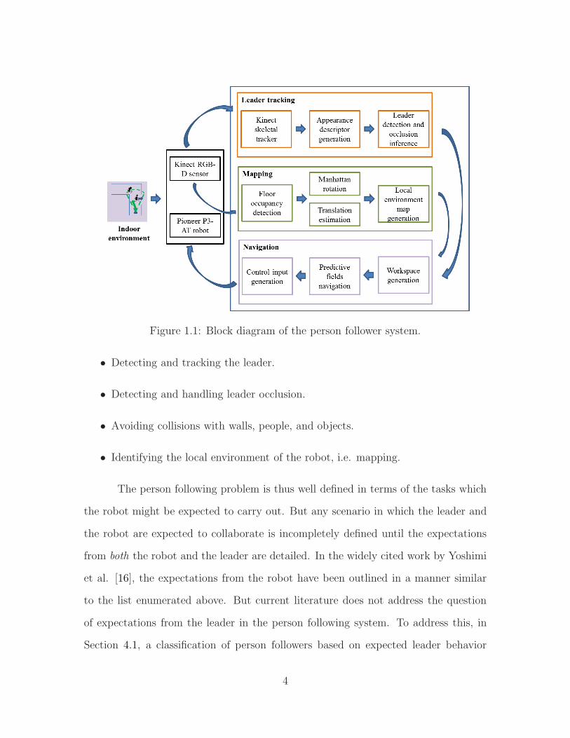
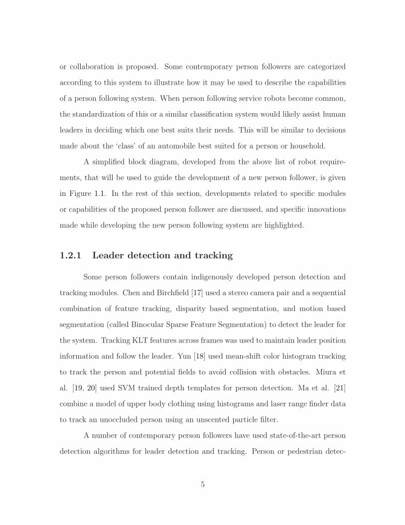
Figure 1.1: Block diagram of the person follower system.

• Detecting and tracking the leader.

• Detecting and handling leader occlusion.

• Avoiding collisions with walls, people, and objects.

• Identifying the local environment of the robot, i.e. mapping.

The person following problem is thus well defined in terms of the tasks which

the robot might be expected to carry out. But any scenario in which the leader and

the robot are expected to collaborate is incompletely defined until the expectations

from both the robot and the leader are detailed. In the widely cited work by Yoshimi

et al. [16], the expectations from the robot have been outlined in a manner similar

to the list enumerated above. But current literature does not address the question

of expectations from the leader in the person following system. To address this, in

Section 4.1, a classification of person followers based on expected leader behavior

4

or collaboration is proposed. Some contemporary person followers are categorized

according to this system to illustrate how it may be used to describe the capabilities

of a person following system. When person following service robots become common,

the standardization of this or a similar classification system would likely assist human

leaders in deciding which one best suits their needs. This will be similar to decisions

made about the ‘class’ of an automobile best suited for a person or household.

A simplified block diagram, developed from the above list of robot require-

ments, that will be used to guide the development of a new person follower, is given

in Figure 1.1. In the rest of this section, developments related to specific modules

or capabilities of the proposed person follower are discussed, and specific innovations

made while developing the new person following system are highlighted.

1.2.1 Leader detection and tracking

Some person followers contain indigenously developed person detection and

tracking modules. Chen and Birchfield [17] used a stereo camera pair and a sequential

combination of feature tracking, disparity based segmentation, and motion based

segmentation (called Binocular Sparse Feature Segmentation) to detect the leader for

the system. Tracking KLT features across frames was used to maintain leader position

information and follow the leader. Yun [18] used mean-shift color histogram tracking

to track the person and potential fields to avoid collision with obstacles. Miura et

al. [19, 20] used SVM trained depth templates for person detection. Ma et al. [21]

combine a model of upper body clothing using histograms and laser range finder data

to track an unoccluded person using an unscented particle filter.

A number of contemporary person followers have used state-of-the-art person

detection algorithms for leader detection and tracking. Person or pedestrian detec-

5

tion [22, 23, 24, 25, 26] is an independent research area in computer vision because

of its applicability to automobile systems [27, 28, 29], surveillance [30], gaming [31],

and analytics [32, 33]. These detectors use either image information, 3D, or a combi-

nation of the two to achieve their purpose. Brookshire [34] and Weinrich [35, 36] use

Histograms of Oriented Gradients (HOG) [37] for person detection. HOG, one of the

landmark contributions in person detection, generates image intensity edge descrip-

tors over image regions and compares them to a trained model to detect a human

silhouette. Brookshire [34] develops a system which uses HOG for person detection

and stereo for depth estimation. When the leader is thus localized, a particle filter

is used to track the leader over outdoor trials. Weinrich et al. [35, 36] generate a

SVM decision tree based on HOG detections to detect the upper body orientation of

people.

The advent of real time RGB-D sensors such as the Microsoft Kinect has

introduced new possibilities in the approach towards person detection and tracking.

Depth data, and as a consequence, 3D point clouds, which used to be available only

by using a stereo rig or by learning depth from monocular data [38, 39], are now

available in the form of raw sensor data. In case of the Kinect, depth and image pixel

positions are related to each other through a known transformation, which allows a

correspondence to be established between RGB and D. Xia et al. propose a person

detection system [40] which leverages this richness of Kinect sensor information.

The Kinect SDK contains an implementation of a person detection and track-

ing algorithm proposed by Shotton et al. [31]. The algorithm is trained, using a

deep randomized forest classifier, to detect human body parts using variation in hu-

man depth images without the use of temporal data. Training is carried out on a

large synthetic depth dataset representative of variations in the human shape and

silhouette. A depth feature is generated at each pixel in the image, and is labeled as

6

belonging to one of multiple joints (20) in the human skeletal representation used by

this algorithm. This pixel-wise labeling is used to infer the 3-D position of each joint

in the skeletal representation. Thus, given a single depth image, the Kinect skeletal

tracker is able to deduce the location and pose of a person. The skeletal tracker is

also able to track up to 6 individuals in the field of view of the sensor. The entire

detection and tracking sequence has been shown to run at close to 50 fps on a CPU

in the original paper [31]. Doisy et al. [41] have used the Kinect skeletal tracker in

their person following system.

The Kinect SDK skeletal tracker is a state-of-the-art person tracking tech-

nology of choice for our person following system. Over multiple trials, the skeletal

tracker was found to be reliable and is well within acceptable range of operation for

the person follower described in this dissertation.

Another candidate tracking method, HOG in combination with particle filter-

ing, was also extensively tested. However, HOG detections were less consistent than

skeletal tracker detections, especially when the pose of the person changed. Also,

particle filter tracks were less reliable than the tracking performance of the skeletal

tracker for typical indoor environments with multiple persons walking in front of the

robot. Section 4.2.1 gives more information about the capabilities and output of the

Kinect skeletal tracker.

1.2.2 Occlusion detection and handling

Person detection and tracking systems are not traditionally equipped to handle

occlusions and recover from them, though there are a few exceptions [42, 43]. This

may be because the scope of applications of these systems, e.g. a generic person

counting application in a crowd, may not require assigning ‘identity’ to an individual

7

and maintaining it through occlusions. However, the question of identity is of primary

importance to a person following robot.

Various attempts have been made to ensure that a person follower maintains

leader identity. At one end of this spectrum are systems where it is assumed that

the leader is unoccluded, which gives the person tracking modules a chance to use

motion or color consistency to localize the leader relative to the robot. Yoshimi et

al. [16] demonstrate a person following robot which has the leader in sight at all

times. Brookshire [34] also assumes this condition is met, and focuses on sensor

integration to develop a robot that can follow a person outdoors through variations

in illumination conditions and terrain. Hence, these and other comparable systems

[18, 41] maintain leader identity by assuming that the leader is always visible, and

focus research efforts on other challenges such as motion planning around obstacles

or variability in test conditions.

Some systems forego the condition of constant visibility and use motion or

color information to keep track of the leader through partial or complete occlusions.

Tarokh and Merloti [44] develop a person tracking system which is initialized using a

color patch on the person’s shirt or top. HSI (Hue-Saturation-Intensity) information is

learned from this patch, and in subsequent frames, similar image patches are inferred

as being tracked locations of the person. Their algorithm can track and follow a person

using vision information through partial occlusions, but makes the assumption that no

object of a similar color profile appears in the field of view during a trial. Satake and

Miura [20] developed a person follower which uses depth data and a Support Vector

Machine (SVM) based verification system to detect people, and leader occlusion is

inferred using a difference in leader and occluding person depth. EKF (Extended

Kalman Filter) is used for tracking the leader, and once the detected occlusion has

passed, leader tracking and following resumes.

8

Tracking capabilities of the Kinect skeletal tracker are limited in the same

sense as many other person tracking systems, i.e. to situations when the person is

unoccluded. If a person is occluded and reappears, the skeletal tracker can once again

detect and track the person, but it assumes that a new person has appeared in front

of the sensor. There is no attempt to recognize or handle occlusions by reidentifying

a person. However, the skeletal tracker is excellent at detecting and tracking people

in the absence of occlusions.

This reliability in unoccluded tracking is leveraged by the occlusion detection

and handling system proposed in Section 4.2. Skeletal information for the initialized

robot leader is augmented with a color descriptor. The descriptor is built using

HSI and L*a*b* (CIE 1976) color spaces, and extracts color values for each bone

detected by the tracker. In each frame, a descriptor is generated for the tracked leader

and compared with the initialized descriptor to confirm that the skeletal tracker has

correctly kept track of the leader. When the skeletal tracker reports a lost skeletal

track, descriptor matching takes over and the robot moves to the last observed leader

location in an attempt to reacquire the leader and overcome occlusion. Unlike motion

based occlusion handling approaches, the duration of the occlusion is inconsequential.

This ability to overcome occlusions of arbitrary period is very useful for prac-

tical human populated environments. Using motion consistency or history to detect

the position of the leader is possible only in a limited sense. A simple sequence of

events such as the leader pausing when occluded or moving in an entirely different

direction can lead to tracking errors in motion-dependent methods. The appearance

based occlusion detection and handling method is thus capable of detecting occlu-

sions and recovering after they have been removed. The actual process of overcoming

occlusions is carried out by the path planning and navigation module of the system.

9

1.2.3 Robots in populated environments

Robot navigation in sparsely populated indoor environments may be consid-

ered to be a subset of the general topic of robot navigation through crowds, which

has seen interest in recent literature. Treuille et al. [45] modeled large crowds in a

simulated environment. A dynamic potential field method was used to move indi-

vidual agents in the crowd. This work was later used by Henry et al. [46] as the

test environment for their work on robot crowd navigation. Reinforcement learning

was used to teach the robot the ‘correct’ method of navigating crowds. After the

learning phase was complete, a robot used Gaussian processes to make navigation

decisions during runtime. Trautman and Krause [47] also explored the problem of

dense crowd navigation using Gaussian processes which modeled interaction between

people in crowds to plan a path for the robot in such an environment. Ziebart et al.

[48] also demonstrated a robot crowd navigation method for a known workspace, in

which data learned over many days is used to infer a motion cost function for places

within that environment.

Some of the principles of crowd navigation find an analog in solutions for per-

son following in populated environments. The most important of these might be

considered to be a representation of the motion of humans in the scene to improve

the robot’s navigation algorithm. Bennewitz et al. [49] learn typical motion patterns

of people using a combination of the Expectation Maximization (EM) algorithm with

Hidden Markov Model (HMM) used for predicting the person’s position. These fore-

casted person trajectories are used by the A* algorithm [50] for robot navigation.

Weinrich et al. [35] track person motions using a 9-D Kalman filter and project robot

and person positions into the future to determine a cost function to help the robot

avoid the path of the approaching human. After every interaction, the robot updates

10

parameters of its cost function to keep learning human behavior to improve collision

avoidance in the future.

The ability of the robot navigation algorithm to plan a path for the robot

after incorporating obstacle motion is very relevant for person followers. It allows

the robot to stay at a safe distance relative to other humans while it is navigating

towards its leader. However, a number of contemporary person followers do not

encode such information in their path planning or navigation modules [16, 18, 41],

primarily because the obstacles in question are assumed to be static objects such as

furniture or boxes on the floor.

The navigation objectives of a mobile robot person follower in indoor environ-

ments may be stated as follows:

• Keep a fixed position relative to the leader.

• Identify obstacles (moving or stationary) which may hinder a direct route to

leader.

• Plan a path around obstacles, while avoiding collision with them.

One of the challenges for mobile robot navigation with an onboard camera

is the question of self-localization. The robot needs to know where it is situated

relative to an absolute coordinate system. Such a representation can be generated

by means of a local map of the environment, in which the view of the environment

at each frame is stitched together based on an estimate of robot motion between

frames. This problem of map generation is commonly called SLAM (Simultaneous

Localization and Mapping). A detailed tutorial on the SLAM problem and relevant

literature was prepared by Bailey and Durrant-Whyte [51, 52].

Using an RGB-D sensor, the SLAM problem is most commonly solved by

using calibrated vision inputs or by using depth-only cues. When calibrated vision

11

inputs are used, the technique for map generation is called visual odometry [53,

54]. Inter-frame correspondence is established using feature correspondences, and

knowing the depth to each feature, corresponding 3-D points can be estimated. These

correspondences are then used to estimate inter-frame transformations using a method

such as least squares [55] or Iterative Closest Point [56]. Alternately, depth data may

be used to generate 2-D scans, which can then be compared using scan matching

techniques [57, 58] to estimate inter-frame transformations.

Some of the commonly used SLAM techniques assume sufficient information

in the environment for correspondence based techniques to be successful. Indoor hall-

ways, in which our system is intended to be used, do not provide consistent richness

in texture or depth variations for either the visual odometry or scan matching tech-

niques to generate consistently accurate estimates. To cope with this, the proposed

system uses a combination of Manhattan rotation estimates [59, 60] with translation

estimates from dead reckoning to generate a map of the robot’s environment. To get

Manhattan rotation estimates, lines are detected in a 2-D scan of the workspace and

a dominant direction for these lines is inferred. This dominant direction is compared

with a reference which is established in the map initialization frame. The Manhat-

tan assumption is that lines in an indoor environment are orthogonal to each other.

This property is used to estimate frame by frame rotation. Section 4.3 explains this

mapping technique.

To satisfy the requirements for path planning, the classic navigation function

method [61] is chosen for our system, the history of its development explained, and the

research contributions relative to its modification are highlighted in the next section.

12

1.2.4 Navigation function path planning

In the work proposed here, the ‘predictive fields path planner’, an extension of

navigation function path planning, is developed. Navigation functions, in turn, are a

special type of potential fields path planner.

In a seminal article, Khatib [62] introduced potential fields path planning in

robotics. The simple yet powerful idea which formed the basis of this paper was

a topological representation of the robot workspace in which the robot was being

attracted to its goal position and repelled by obstacles. Attraction and repulsion

were both forces which were acting on the robot ‘virtually’, and the actual steering

input to the robot to the goal was calculated simply as the net force acting on it at

any given time. In effect, the workspace was pervaded with potential fields, such as

the attractive well at the goal position and the high potentials at obstacle boundaries.

The potential field approach was adopted rapidly, and its variations used in

other well known robot navigation methods such as the schema approach by Arkin

[63] and the generalized potential field method of Krogh and Thorpe [64]. However, in

1991, Koren and Borenstein [65] provided a mathematical analysis of the weaknesses

of the potential field method. In their work, they identified the following major

problems with potential fields, paraphrased here from their paper:

• Local minima, where attractive and repulsive forces cancel out, exist.

• If obstacles are closely spaced, there is no path between them to goal.

• Robot oscillates close to obstacles and narrow passages between obstacles.

Despite this set of limitations, potential fields retain their appeal in robotics because

of the speed and simplicity of their implementation. They have been used in subse-

quent robotics literature with some modifications, e.g. using a composite of various

13

potentials to drive the robot [66] or defining potentials such that robot can converge

to goal in the presence of nearby obstacles [67].

Using the idea of topological representation of the workspace to create naviga-

tion gradients for the robot, Rimon and Koditschek, in a series of papers [61, 68, 69,

70] introduced the idea of navigation functions. Navigation functions path planning

is an integrated path planning, motion planning, and controls approach in which the

following mathematical guarantees are shown to exist:

• Only a single global minimum exists at the goal position.

• Robot avoids collisions with obstacles.

• Robot stays within the boundary of the workspace.

In Section 2.1 details of the navigation function formulation have been provided.

Because of their mathematical guarantees and the simplicity in their formulation,

navigation functions were chosen as the path planning basis for our system. However,

a number of modifications needed to be made to the framework to make it useful in

real-world applications.

Since their introduction, navigation functions have been used in multi-agent

robot simulations [71, 72] and in collision avoidance for articulated non-holonomic

robots [73]. However, they have seen only limited experimental usage [74, 75] for two

reasons:

• Highly variable magnitude of control inputs generated for the robot.

• Practical workspaces need to be transformed to circular workspaces before nav-

igation functions can be used.

In Section 2.3, a normalized control input is developed and it is shown that this input

yields a stable navigation system. In Section 2.4, a practical workspace representation

14

is proposed. This representation obviates the need for estimating transformations to a

circular world, which are typically difficult to find for practical geometries. A similar

effort has been made by Filippidis and Kyriakopoulos [76], who extend the utility of

navigation functions to curved, non-circular worlds, and who use normalized control

inputs in [77].

With the mechanism for using navigation functions in practical environments

in place, the need to incorporate obstacle motion into the path planning framework

for a robotic person follower can be addressed. Navigation functions in their original

form [61] were designed for use in static environments. However, it was shown math-

ematically by Chen et al. [72], and experimentally by Widyotriatmo and Hong [74]

that the stability of this path planner is not affected by its use in dynamic obstacle

environments. Hence, in our own previous work [78, 79], we used a modification of

navigation functions called ‘predictive fields path planning’ to incorporate the motion

of obstacles into the navigation function path planner. To do this, each obstacle with

an ellipse which is representative of its direction of motion and velocity along that

vector. Then, the repulsion felt by the robot from an obstacle was characterized by

a function of the actual obstacle position and its predicted path inside its elliptical

envelope. This formulation has echoes of the concept of ‘danger’ posed by an ob-

stacle’s motion, which has been used in the context of potential fields path planning

[80, 81, 82, 83]. The elliptical field formulation and its simulation results are presented

in Sections 2.2.1 and 2.2.4, respectively.

The elliptical field formulation was tested experimentally using a non-person

following robot before it was integrated into the person follower system. This was

a significant step in the development and prototyping of this path planner and, as

mentioned earlier, one of the first demonstrable experimental results for navigation

function path planning. The details of this experimental setup have been covered in

15

Chapter 3.

Finally, the predictive fields path planner was prototyped as a system module

in the person follower in Section 4.4.3. In addition to the modifications to navigation

functions described earlier, another modification was required for such a system,

i.e. the ability to systematically cope with a moving target. This is because classic

navigation functions assume a fixed goal position. The description of a workspace

generation method which works around this limitation is given in Section 2.4.

In summary, a robotic person follower system was equipped with the ability

to detect leader occlusions and overcome them using an indigenously developed path

planner. The organization of the document is briefly reviewed in the next section.

1.3 Dissertation outline

In Chapter 2, the theoretical development of predictive fields path planning is

motivated and explained. The assumptions and predicted performance are compared

and contrasted with the original navigation functions path planning. Simulation

results are provided to demonstrate the utility of this path planning framework.

In Chapter 3, the experimental results for predictive path planning tests with

a non-person follower is detailed. Various modules of the system, including sensing,

hardware and software interfacing, and navigation are explained.

In Chapter 4, the Kinect skeletal tracker, appearance descriptor for the leader,

and mapping module which localizes the robot and feeds the path planner, are de-

scribed. Proof of concept experimental results for the use of predictive fields path

planning are provided.

Finally, in Chapter 5, results from the previous chapters are summarized and

possible future directions for this research topic are discussed.

16

Chapter 2

Development of predictive fields

path planning

The conceptualization and theoretical development of predictive fields path

planning is presented in this chapter. Predictive fields build upon the seminal work

of navigation function path planning by Rimon and Koditschek [61, 68, 69, 70]. Nav-

igation functions, in turn, were influenced by the work of Khatib [62], in which the

robot was guided to the goal position using a net driving force that was the vector

sum of an attractive force to the goal and repulsive forces away from obstacles. Navi-

gation functions are a compelling path planning solution because of the mathematical

guarantee of convergence to goal. However, certain requirements and features of this

method make it untenable for practical applications, including:

• Navigation functions are only proven to work for workspaces containing static

obstacles.

• Navigation function path planners may generate impracticably large velocity

inputs to the robot, created on account of a large scaling gain in the formulation.

17

• Navigation functions can be applied to real workspaces only after estimating a

complicated geometric transformation called the star world transformation.

• Navigation functions can only be applied when the goal position is static.

In this chapter, methods to address each of the above limitations of the classic

navigation function approach are presented [78, 79]. The term ‘predictive fields’, used

to describe this modified navigation function method, alludes to the use of envelopes

around moving obstacles to allow the robot to leverage obstacle motion information

in the path planning paradigm. A stable, normalized velocity controller is proposed

to obviate the need for the scaling gain and, in turn, for large input velocities. Finally,

a new representation of workspaces circumvents the requirement to find complex star

world transformations for workspaces. This representation has the added feature of

being usable when the goal position for the robot is moving, a condition disallowed

by the navigation function path planner.

This chapter begins with a review of the navigation function method and

subsequent sections present the predictive fields approach and its results.

2.1 Navigation function path planning

The theory of navigation function path planning was proposed in a series

of papers by Rimon and Koditschek [61, 68, 69, 70]. The eponymous ‘navigation

function’ in this path planning method was a mathematical construct which pushed

the robot to its goal position and away from obstacles. Certain information about

the system was assumed to be available for path planning. The known information

included:

• The position and size of the robot,

18

• The position and size of each obstacle,

• The location of the goal position for the robot, and

• The size of the workspace, assuming that the workspace at least encompassed

the robot, goal, and all obstacles.

Assuming this information, the navigation function path planner was formulated to

achieve the following objectives:

• Objective 1: The robot position was constrained to always lie within its

workspace,

• Objective 2: The robot avoided collisions with all obstacles in the workspace,

and

• Objective 3: The robot reached its goal position.

Given this setup, the authors proved that the navigation function, when con-

structed following a set of mathematical constraints, guaranteed convergence to the

goal for any initial configuration.

2.1.1 The navigation function

The form of the navigation function was defined by Rimon and Koditschek

[61, 68, 70] as follows. Let q ∈ R1×2 denote robot position. Let q∗ ∈ R

1×2 be the goal

point in the interior of a robot free configuration space F . A map ϕ : F → [0, 1] is

defined to be a navigation function if it is

• analytic on F ,

• polar, with a unique minimum at q∗,

19

• admissible on F , and

• a Morse function.

Mathematically, a solution is proposed as

ϕ (q) =Ks ‖q − q∗‖2

[

‖q − q∗‖2k +G (q)]1/k

, (2.1)

where k ∈ N is called the navigation gain, and Ks ∈ R is an unknown scaling factor

between the dimensionless navigation function and units of the practical environment.

The term G , G0G1 ∈ R is a composite of workspace envelope avoidance (G0) and

obstacle avoidance (G1) functions. The scalar functions G0, G1 ∈ R are defined as

follows

G0 (q) = β0(q)

G1 (q) =n∏

i=1

βi (q)(2.2)

where β0 and βi are repulsion terms for workspace envelope and obstacles, respectively,

and are discussed in subsequent sections. To converge to goal, the robot navigates

along the gradient of the navigation function (2.1).

The destination of the robot, q∗, is assumed to be static and within the

workspace. It has to be noted that the requirement of the goal position to be static

makes it impossible to use this path planning approach for the motivating applica-

tion, i.e. person following. For use in a practical situation, it is necessary to represent

leader motion in such a way that the static goal requirement is not violated.

20

2.1.2 An overview of repulsion functions

Repulsion terms (2.2) of the navigation function (2.1) are designed to steer

the robot away from the workspace envelope and other obstacles. They have been

called ‘obstacle functions’ in literature [61]. Note that the workspace envelope itself

is an ‘obstacle’ the robot must avoid, even though it may not have a physical pres-

ence in the environment. The terminology is changed here to ‘repulsion function’ to

avoid confusing the workspace envelope with obstacles inside it. The envelope of the

workspace is referred to as the ‘workspace envelope’ from here on, and ‘obstacles’

refers to the objects that lie inside the boundary, after the robot and its goal position

are excluded from the list.

These functions need to follow the simple rule that their value is zero at the

boundary of the obstacle and at the workspace envelope, i.e. when the robot touches

either, and non-negative otherwise. This rule allows for repulsion functions to be

formulated using different types of smooth curves. One of the research contributions of

the predictive fields formulation is to identify the means by which repulsion functions

for obstacles can be changed to account for the motion of these obstacles.

2.1.3 Repulsion function - workspace envelope

The formulation used for workspace envelope repulsion is derived from the

work of Chen et al. [72, 84, 85]. If the robot is sufficiently distant from the workspace

envelope, the boundary repulsion term does not contribute to the navigation function,

i.e. β0(q) = 1. When the robot of radius r comes within a distance rs of the envelope,

rs > r, the repulsion term begins to contribute to the navigation function until, at

the point of contact, this value reduces to 0 as per the requirements of repulsion

functions. The transition of the function’s value from 1 down to 0 is represented by

21

0 0.5 1 1.50

0.5

1

1.5

x

ρ x

x = h

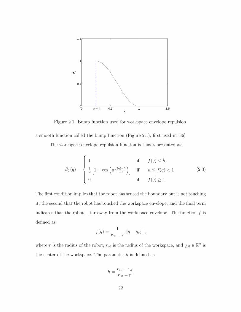
Figure 2.1: Bump function used for workspace envelope repulsion.

a smooth function called the bump function (Figure 2.1), first used in [86].

The workspace envelope repulsion function is thus represented as:

β0 (q) =

1 if f(q) < h.

12

[

1 + cos(

π f(q)−h1−h

)]

if h ≤ f(q) < 1

0 if f(q) ≥ 1

(2.3)

The first condition implies that the robot has sensed the boundary but is not touching

it, the second that the robot has touched the workspace envelope, and the final term

indicates that the robot is far away from the workspace envelope. The function f is

defined as

f(q) =1

ro0 − r‖q − qo0‖ ,

where r is the radius of the robot, ro0 is the radius of the workspace, and qo0 ∈ R2 is

the center of the workspace. The parameter h is defined as

h =ro0 − rsro0 − r

,

22

where rs is the distance from the robot within which the repulsive term is activated.

Since r < rs < ro0, 0 ≤ h < 1. This formulation describes the bump function curve

seen in Figure 2.1.

2.1.4 Repulsion function - obstacles

It is assumed that the workspace contains all interior obstacles and the robot

and goal positions. Past work on designing interior obstacle repulsion functions [61,

72] uses the quadratic form:

βi =[

‖q − qoi‖2 − (r + roi)2]

(2.4)

where qoi ∈ R+ is the center and roi ∈ R

+ the radius of the ith obstacle. When the

robot and obstacle touch, the value of βi goes to zero as per the requirement of the

beta function. As defined earlier, r is the radius of the robot and q is its position in

the workspace.

The weaknesses of this formulation are discussed in Section 2.2 and an im-

proved formulation is discussed in the same section.

2.1.5 Navigation inputs to robot

It is assumed [72] that the robot can be described by the following kinematic

model

q = u, (2.5)

where u ∈ R2 is the control input to the robot, given by

u = −K

(

∂ϕ

∂q

)T

, (2.6)

23

−60 −40 −20 0 20 40 60−60

−40

−20

0

20

40

60

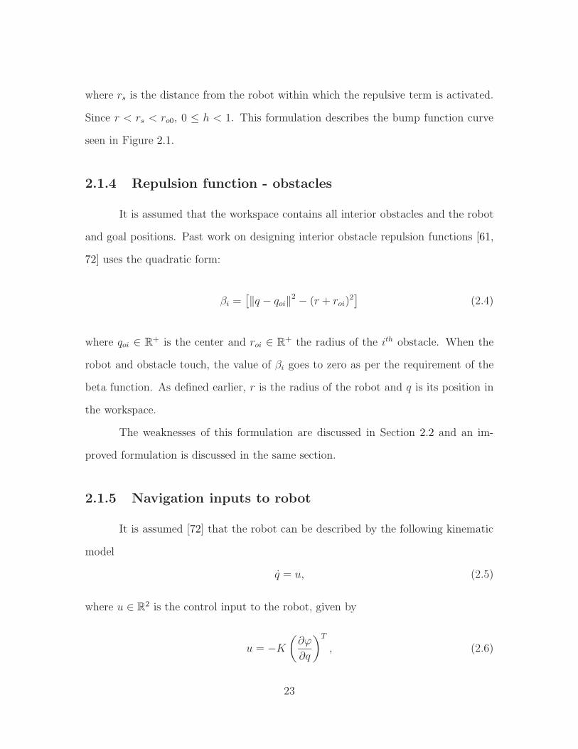
Figure 2.2: Path to goal using standard navigation functions.

The robot, marked using blue circles, approaches the goal, marked using a black square, inthe presence of three stationary obstacles, marked using red circles. During this straightline traversal to goal, the robot stays within bounds of the workspace, marked using a

black circular envelope.

Eq. (2.6) commands the robot to descend down the slope of the navigation

function to its goal position. Though Rimon and Koditschek prove that this guar-

antees a global minimum exists at the goal which the robot will eventually reach,

it requires accurate tuning of a few very sensitive parameters. Consider a relatively

simple setup demonstrated in Figure 2.2 and tested using MATLAB Simulink. The

robot has a clear path to goal (marked by the black square) in the presence of three

obstacles (red circles), and it follows this path as indicated by the blue circles. How-

ever, this particular behavior could be observed only after the navigation gain k (from

(2.1)) was heuristically tuned to a value of k = 20, and the controller gain K (from

(2.6)) was tuned to the very large and quite unintuitive value of K = 1.2 exp 14.

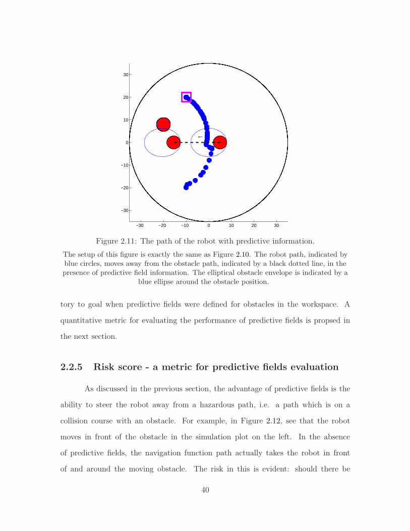
Velocity inputs to the robot are seen in Figure 2.3, with the red lines representing x

24

Figure 2.3: High velocity inputs to robot.

Using the standard form of navigation functions, the robot receives navigation inputs ofunpredictable magnitude. Red lines show x inputs and black lines show y direction inputs.

velocity inputs and black lines representing y velocity inputs. As seen for this trial,

and typically observed in most trials, these values were found to be very high, in the

hundreds or greater. Such inputs are not directly usable as an input to a practical

mobile robotic platform during experiments. Finding the right combination of k and

K was found to be a time consuming process with no real payoff at the end in terms

of getting a usable velocity control input for the mobile robot. Hence, an improved

control input was desirable for this form of the navigation function path planner.

Such an input is proposed in Section 2.3.

2.1.6 Star world transformation

For the original Rimon-Koditschek formulation to be usable in a practical

workspace, the workspace has to satisfy the definition of a ‘star world’. A workspace

is defined to be a star world if it contains a point called a ‘center point’ in [61]. Rays

25

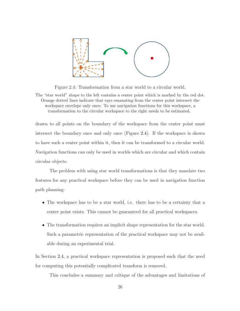
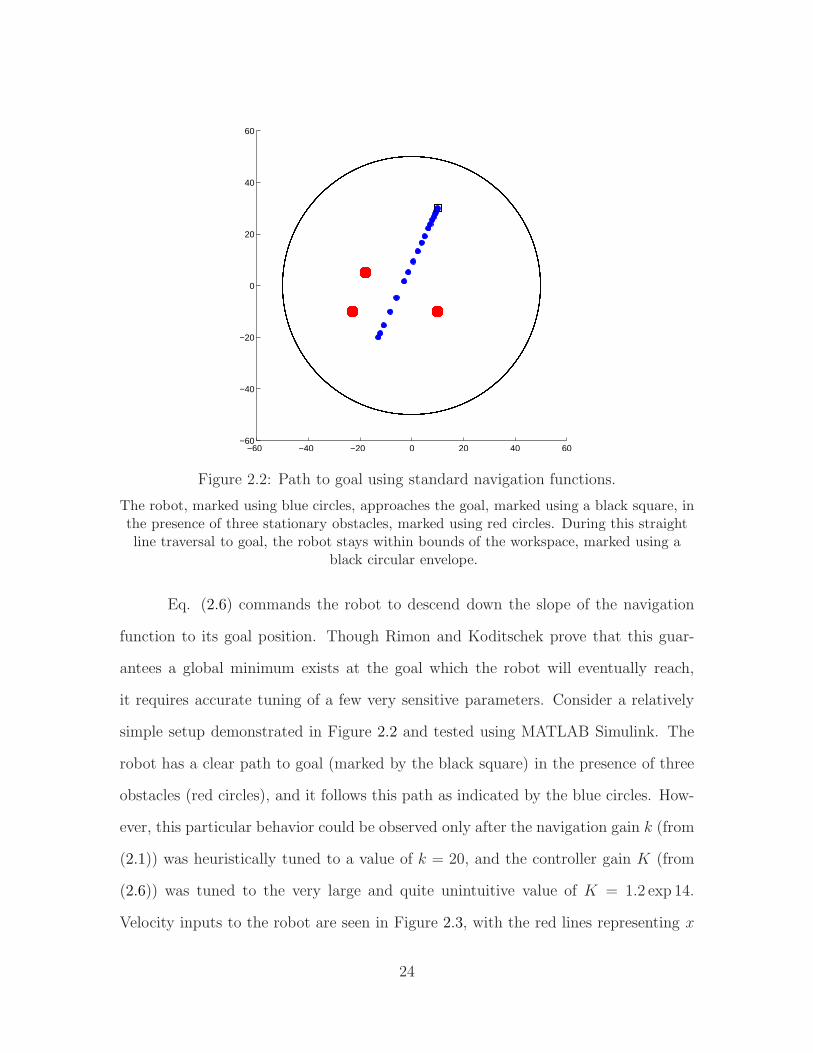
Figure 2.4: Transformation from a star world to a circular world.

The “star world” shape to the left contains a center point which is marked by the red dot.Orange dotted lines indicate that rays emanating from the center point intersect theworkspace envelope only once. To use navigation functions for this workspace, atransformation to the circular workspace to the right needs to be estimated.

drawn to all points on the boundary of the workspace from the center point must

intersect the boundary once and only once (Figure 2.4). If the workspace is shown

to have such a center point within it, then it can be transformed to a circular world.

Navigation functions can only be used in worlds which are circular and which contain

circular objects.

The problem with using star world transformations is that they mandate two

features for any practical workspace before they can be used in navigation function

path planning:

• The workspace has to be a star world, i.e. there has to be a certainty that a

center point exists. This cannot be guaranteed for all practical workspaces.

• The transformation requires an implicit shape representation for the star world.

Such a parametric representation of the practical workspace may not be avail-

able during an experimental trial.

In Section 2.4, a practical workspace representation is proposed such that the need

for computing this potentially complicated transform is removed.

This concludes a summary and critique of the advantages and limitations of

26

the classic navigation function path planner. In subsequent sections, various mod-

ifications to navigation function path planning are proposed. These modifications

address the limitations of the approach outlined in the chapter introduction and in

this section.

2.2 Development of an elliptical repulsion function

The first of the limitations of navigation function path planners is that obstacle

motion is not encoded in them in any manner. In its original form, obstacle repulsion

is defined by Eq. (2.4). The original definition of βi satisfies the requirements of

the repulsion function from Section 2.1.2 and has the favorable property that beta

changes quadratically as the robot moves toward the obstacle. This rate of change

ensures that the robot’s approach to an obstacle’s current position is strongly repelled.

However, this definition does not account for the manner in which an obstacle has

been moving or is expected to move. It does not convey the level of threat posed

by an obstacle to the robot’s approach to the goal. For example, even if the current

position of the obstacle is not between the robot and the goal, is there a chance that

the obstacle will move in between the robot and target at a later instant, when the

robot has moved dangerously close to the obstacle? A solution to this is to represent

the obstacle motion using an elliptical field. This concept was first introduced our

work [79], and has since been subject to rigorous mathematical treatment by Filippidis

and Kyriakopoulos [76], in which it was shown that the entire elliptical envelope can

be used to compute navigation function terms.

27

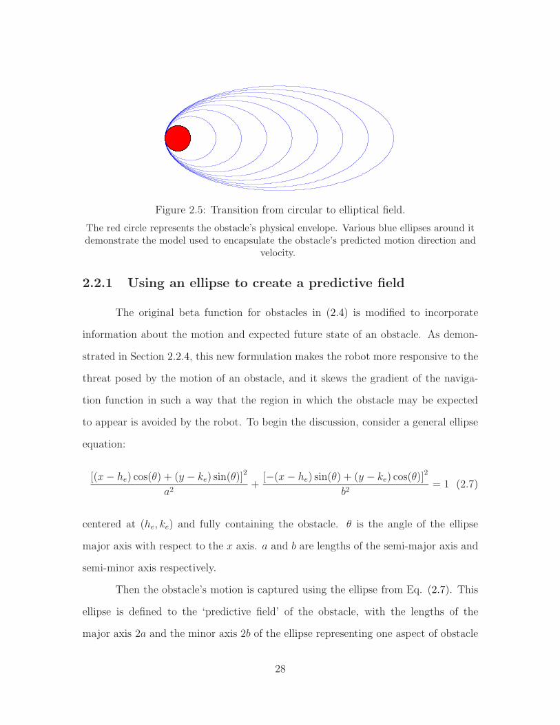
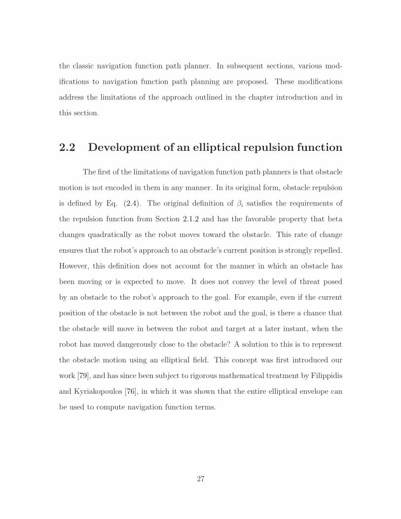
Figure 2.5: Transition from circular to elliptical field.

The red circle represents the obstacle’s physical envelope. Various blue ellipses around itdemonstrate the model used to encapsulate the obstacle’s predicted motion direction and

velocity.

2.2.1 Using an ellipse to create a predictive field

The original beta function for obstacles in (2.4) is modified to incorporate

information about the motion and expected future state of an obstacle. As demon-

strated in Section 2.2.4, this new formulation makes the robot more responsive to the

threat posed by the motion of an obstacle, and it skews the gradient of the naviga-

tion function in such a way that the region in which the obstacle may be expected

to appear is avoided by the robot. To begin the discussion, consider a general ellipse

equation:

[(x− he) cos(θ) + (y − ke) sin(θ)]2

a2+

[−(x− he) sin(θ) + (y − ke) cos(θ)]2

b2= 1 (2.7)

centered at (he, ke) and fully containing the obstacle. θ is the angle of the ellipse

major axis with respect to the x axis. a and b are lengths of the semi-major axis and

semi-minor axis respectively.

Then the obstacle’s motion is captured using the ellipse from Eq. (2.7). This

ellipse is defined to the ‘predictive field’ of the obstacle, with the lengths of the

major axis 2a and the minor axis 2b of the ellipse representing one aspect of obstacle

28

motion information each. When the obstacle is either known to be stationary or

nothing is known about its motion, the ellipse collapses into a circle the size of the

obstacle to indicate no motion information. As we learn (based on estimates from

the vision system) the motion of the obstacle, the circle is skewed in the direction of

motion. Therefore, the direction of the major axis indicates the estimated direction of

motion, and the length of the major axis indicates the estimated speed. The length

of the minor axis then indicates the uncertainty in the direction estimate. Thus,

various scenarios are captured by the construction of this elliptical field, enabling it

to explain the influence of predictive fields in potential field based path planning.

Typical evolution of the elliptical field is illustrated in Figure 2.5.

It is assumed that sensors and algorithms working in parallel with the path

planner can track objects, quantify their behavior, and uses this data to provide

suitable values of a and b to guide the path planner. In case the sensing system is

not sufficiently sophisticated to provide these values, a fixed-size ellipse could also be

used on the basis of motion history.

2.2.2 Constraints on the size of the ellipse

The elliptical predictive field is an estimate of where we expect the obstacle

to be at a future time instant. This estimate should obviously contain the current

position of the obstacle, so its radius should not extend outside the perimeter of the

ellipse. If the obstacle of radius ro is placed at the focus of the ellipse, then this means

that the radius of the obstacle should be less than the periapsis (the smallest radial

distance) of the ellipse:

ro ≤ a−√a2 − b2, (2.8)

29

which rearranging terms yields a constraint on the length of the minor axis:

b ≥√

ro (2a− ro).

The limiting case of (2.8) is when the ellipse is a circle, i.e., a = b. This leads to the

following constraint on the length of the major axis:

a ≥ ro.

2.2.3 Formulation of repulsion function

Now that the elliptical field has been defined to capture motion trends of an

object, the repulsive term in (2.4) needs a redefinition to leverage this information.

It needs to be noted that the ellipse is a likely region for the presence of the obstacle,

and the robot is allowed to be inside the ellipse as long as the robot does not touch

the measured position of the obstacle. The requirement that βi should go to zero

on physical contact between the robot and obstacle still needs to be obeyed, and the

robot should be repelled from the obstacle at any other position in the workspace,

whether inside or outside the ellipse.

In addition to the above observations, the following requirements are intro-

duced for beta redefinition:

• The elliptical predictive field should provide the obstacle’s repulsive force when

the robot is outside the ellipse.

• The circular formulation from Eq. (2.4) should come into play only when the

robot is inside the ellipse.

30

A modified beta function is proposed as follows:

βi =

0 robot touches the boundary of an obstacle

βci robot is inside the ellipse

βei robot is outside the ellipse

(2.9)

where βei is the beta function for the robot with respect to the ellipse around the ith

obstacle. The obstacle is located at one focus of the ellipse defined in Eq. (2.7). Let

this position be qoi . The obstacle is expected to move along the major axis in the

direction of motion to arrive at its predicted position q′oi at a future time instant t′.

Figure 2.6: A sample robot approach to obstacle ellipse.

Overlapping green circles indicate a sample approach path of the robot. The obstacleposition (red circle) is projected along the major axis of the ellipse to its predicted

position (black circle). When outside the ellipse, the black circle is used for computingobstacle repulsion term. When the robot enters the uncertain elliptical field, the actual

position of the obstacle is used to compute obstacle repulsion.

Then βei is defined as

βei(q) =∥

∥q − q′oi∥

∥

2 − (r + dei)2 + δ, (2.10)

31

where dei is the distance from the predicted obstacle position q′oi to the point qrei

where the line joining the robot position q and the predicted position of the obsta-

cle q′oi intersects the ellipse. Various positions of the robot (indicated by the green

intersecting circles) as it approaches the obstacle along a straight line are plotted in

Figure 2.6. The left focus of the ellipse (red) is the actual obstacle position, the right

focus (black) is the most likely predicted position. Points of intersection with the

ellipse are calculated and the point closer to the robot is selected for βe computation.

Note that if we set δ = 0, this formula for βei guarantees that it goes to zero

when the robot touches the outside of the ellipse. The curve described by this formula

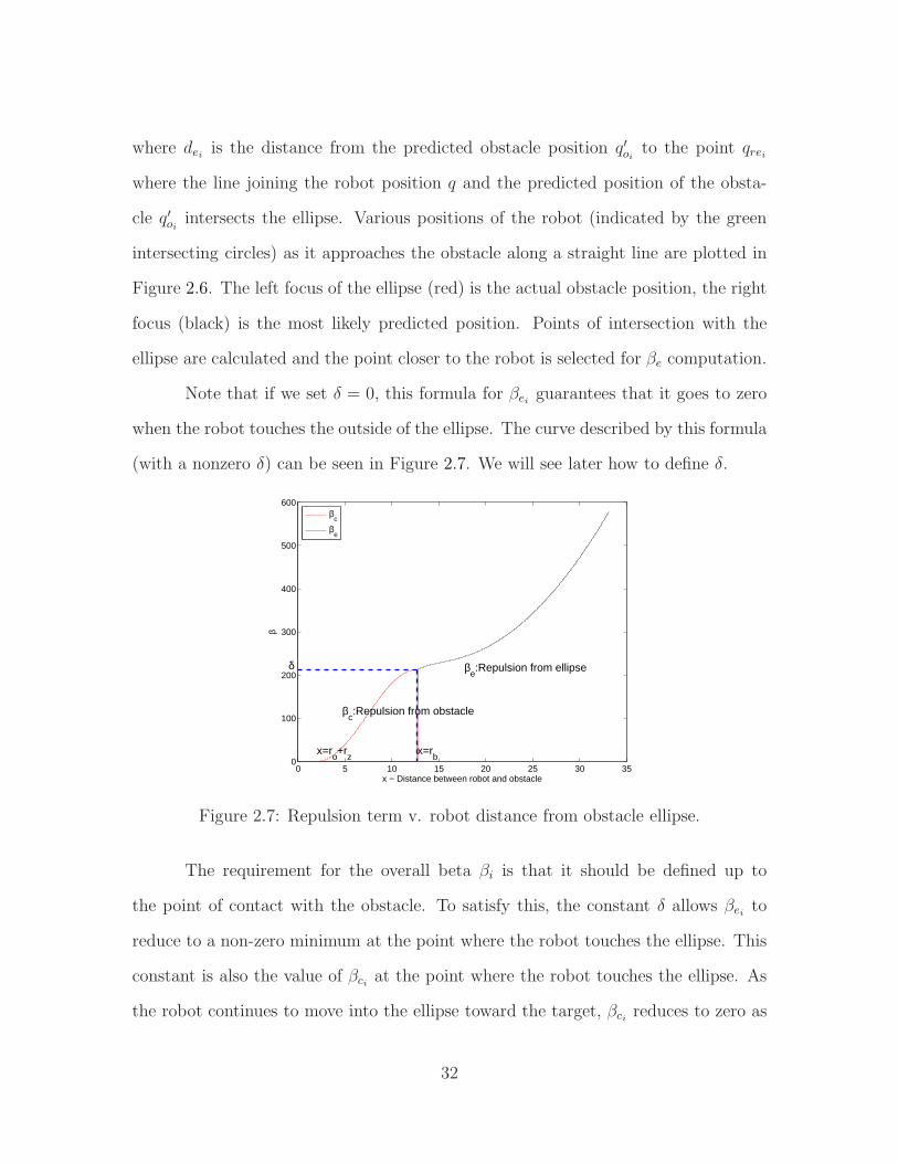
(with a nonzero δ) can be seen in Figure 2.7. We will see later how to define δ.

0 5 10 15 20 25 30 350

100

200

300

400

500

600

x − Distance between robot and obstacle

β

βe:Repulsion from ellipse

βc:Repulsion from obstacle

δ

x=rb

x=ro+r

z

βc

βe

Figure 2.7: Repulsion term v. robot distance from obstacle ellipse.

The requirement for the overall beta βi is that it should be defined up to

the point of contact with the obstacle. To satisfy this, the constant δ allows βei to

reduce to a non-zero minimum at the point where the robot touches the ellipse. This

constant is also the value of βci at the point where the robot touches the ellipse. As

the robot continues to move into the ellipse toward the target, βci reduces to zero as

32

desired. The βci curve should be continuous with respect to the βei curve to make the

resultant beta differentiable throughout its domain. This curve is plotted in Figure

2.7.

The requirements of the function βci are:

• The function should reach its maximum value at the boundary of the ellipse,

i.e., when∥

∥q − q′oi∥

∥ = (r + dei).

• The function should reach its minimum value of zero when the robot and the

obstacle touch, i.e., when ‖q − qoi‖ = (r + roi).

• The maximum value of the function should be given by the βci value when the

robot touches the ellipse along a straight line approach to the obstacle. Let

this point be qrei. This gives δ a constant value relative to the line of approach

δ = ‖qrei − qoi‖2 + (r + roi)2. This constant value is added to the ellipse beta

when the robot is outside the ellipse, and accounts for the movement of the

robot inside the elliptical predictive field.

• Additionally, the addition of delta to βei ensures that the obstacle beta con-

straint, i.e., beta goes to zero only when the robot and obstacle physically

touch, is satisfied even with the addition of the ellipse to the formulation.

This is accomplished by using a mirror image of the bump function [86], since the

highest point on the curve needs to be further away from the x axis.

Given the above constraints, let the following terms be defined:

rb = ‖qrei − qoi‖ − (roi + r)

hc = roi + r

δ = ‖qrei − qoi‖2 − (r + roi)2 ,

33

where:

• rb - range of the bump function, or the x coordinate where it attains its maxi-

mum

• hc - zero point of the bump function relative to distance of the robot from

obstacle

• δ - maximum value of the bump function, added to the ellipse beta

An additional point has to be made about qrei. Outside the ellipse, the point

of intersection of the robot and the ellipse, of the two possible points of intersection,

is the one closer to the robot. To calculate the bump function value inside the ellipse,

the definition of the point of intersection needs a slight change. As the robot moves

closer and closer to the obstacle, it is possible that the point of intersection on the

other side of the obstacle is the nearer point of intersection of the robot path with

the ellipse. Retaining the ‘nearest intersection point’ definition will then change δ for

the bump function and the desired shape of the β curve will be lost. To ensure this

does not happen, the unit vector from the obstacle to the robot, nrei, is used. The

point of intersection is then defined as the one which is along the vector nrei.

The bump function is then defined as:

βci(x) =

1 rb ≤ x

0 0 ≤ x < hc

δ2

[

1− cos(

π x−hc

rb−hc

)]

hc ≤ x < rb

(2.11)

The bump function then gets the following values. At x = hc, the obstacle and robot

touch and βci goes to zero. At x = rb, the elliptical predictive field and the robot

touch and βci gets its maximum value of δ. Beyond rb, the maximum value of the

34

βci term, δ, adds to the βei term which begins to dominate the overall β function.

Therefore the value of βei approaches δ instead of 0 as the robot moves towards the

ellipse.

With these definitions for βci and βei, the overall definition of βi (2.9) is con-

sistent with the requirements of the repulsion function. In the next section, the

qualitative effect of this redefinition of the repulsive term on robot navigation can be

seen.

35

2.2.4 Effect of new repulsion function on robot path

−30 −20 −10 0 10 20 30

−30

−20

−10

0

10

20

30

→

Figure 2.8: The path of the robot without predictive information.

The robot path, indicated by blue circles, approaches the obstacle path, indicated by ablack dotted line, in the absence of predictive field information. The moving obstaclemoves left to right, from the left end of the black dotted line, to the right, and its startand end positions are both shown by red circles. A stationary obstacle, shown by a red

circle, sits at (−20, 8) throughout the simulation.

MATLAB Simulink (Mathworks Inc., Natick, MA) was used to simulate the

proposed change to the repulsion function and to qualitatively compare it against

previous results from Chen et al. ([72, 84, 85]). Such a comparison is easily possible

because the predictive field reduces to the obstacle’s circular envelope when motion

information is not used, and Eq. (2.10) reduces to Eq. (2.4). The hypothesis to be

tested is: using predictive fields makes it possible for the robot to converge to the

target following more effectively than using the original navigation function formula-

tion from Rimon and Koditschek. This also implies that the robot is pushed away

from the predicted path of the obstacle, thus driving it to goal using a less dangerous

36

−30 −20 −10 0 10 20 30

−30

−20

−10

0

10

20

30

→

Figure 2.9: The path of the robot with predictive information.

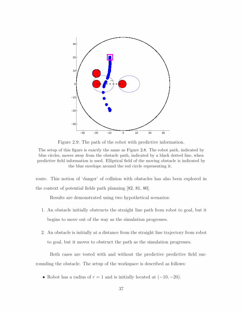
The setup of this figure is exactly the same as Figure 2.8. The robot path, indicated byblue circles, moves away from the obstacle path, indicated by a black dotted line, whenpredictive field information is used. Elliptical field of the moving obstacle is indicated by

the blue envelope around the red circle representing it.

route. This notion of ‘danger’ of collision with obstacles has also been explored in

the context of potential fields path planning [82, 81, 80].

Results are demonstrated using two hypothetical scenarios:

1. An obstacle initially obstructs the straight line path from robot to goal, but it

begins to move out of the way as the simulation progresses.

2. An obstacle is initially at a distance from the straight line trajectory from robot

to goal, but it moves to obstruct the path as the simulation progresses.

Both cases are tested with and without the predictive predictive field sur-

rounding the obstacle. The setup of the workspace is described as follows:

• Robot has a radius of r = 1 and is initially located at (−10,−20).

37

• The workspace envelope bump function comes into effect at a distance rs = 5.

• Goal is located at (−10, 20).

• Stationary obstacle with radius ro1 = 3 is located at (−20, 8). The stationary

nature of the obstacle causes the predictive predictive field around it to shrink

to a circle with the same radius as the obstacle.

• The workspace is centered at (0, 0) with a radius of ro0 = 35.

• The predictive field of the moving obstacle of radius ro2 = 3 is described by an

ellipse with parameter a = 8 in both cases.

• Gains from Eq. (2.1) and Eq. (2.6) are set at κ = 4.5 and K = 1.2 respectively.

They remain unchanged for the given setup; however, they might need to be

tuned on changing the number of obstacles in the workspace.

In Scenario 1, the obstacle starts at (−20, 0) and travels 20 units in the

workspace at a constant velocity. The sense of its motion is such that it is mov-

ing out of the way of the robot’s path to goal. Without the use of a predictive field,

it can be seen that, in Fig. 2.8, the robot tries to move around the obstacle. This

causes it to move toward the path of the obstacle and forces a correction in its path

approximately midway through its trajectory. However, when the predictive field is

added, the path planner is able to sense that the more optimal path to goal would

actually be behind the obstacle, as seen in Fig. 2.9. The trajectory traced as a result

is much more intuitive than the first case.

38

−30 −20 −10 0 10 20 30

−30

−20

−10

0

10

20

30

←

Figure 2.10: The path of the robot without predictive information.

The robot path, indicated by blue circles, approaches the obstacle path, indicated by ablack dotted line, in the absence of predictive field information. The moving obstaclemoves right to left, moving in the way of the straight line path of the robot to goal. Its

start and end positions are both shown by red circles and direction of motion by the littleblack arrow. A stationary obstacle, shown by a red circle, sits at (−20, 8) throughout the

simulation.

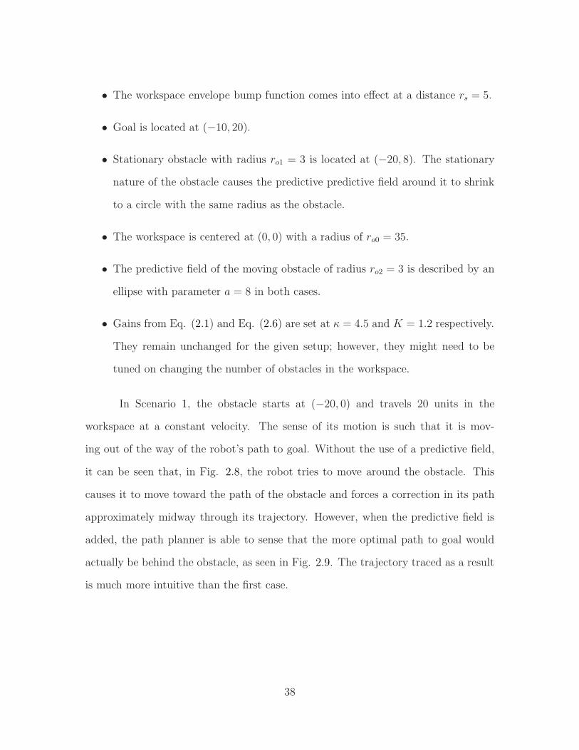
A similar improvement is observed in Scenario 2, when the obstacle starts out

of the way of the robot’s path to goal. Once again, it moves 20 units with a constant

velocity, but this time it moves from right to left. Its motion is such that, relative

to the robot, the robot’s straight line path to goal is obstructed. It is seen that the

robot, when guided by current information alone (Fig. 2.10, initially travels toward

the obstacle, until the repulsion from the obstacle forces a change in its trajectory.

This course correction is averted using predictive fields (in Fig. 2.11), where the

robot’s path is always such that it seeks to avoid the path of the obstacle.

Results from multiple trials corroborated the hypothesis that the robot was

able to successfully converge to the goal while moving along a less dangerous trajec-

39

−30 −20 −10 0 10 20 30

−30

−20

−10

0

10

20

30

←

Figure 2.11: The path of the robot with predictive information.

The setup of this figure is exactly the same as Figure 2.10. The robot path, indicated byblue circles, moves away from the obstacle path, indicated by a black dotted line, in thepresence of predictive field information. The elliptical obstacle envelope is indicated by a

blue ellipse around the obstacle position.

tory to goal when predictive fields were defined for obstacles in the workspace. A

quantitative metric for evaluating the performance of predictive fields is propsed in

the next section.

2.2.5 Risk score - a metric for predictive fields evaluation

As discussed in the previous section, the advantage of predictive fields is the

ability to steer the robot away from a hazardous path, i.e. a path which is on a

collision course with an obstacle. For example, in Figure 2.12, see that the robot

moves in front of the obstacle in the simulation plot on the left. In the absence

of predictive fields, the navigation function path actually takes the robot in front

of and around the moving obstacle. The risk in this is evident: should there be

40

Figure 2.12: Route in absence and presence of predictive fields.

In both images, overlapping black circles are robot positions from the start to the timeinstant at which this snapshot is taken. The plus sign at the top is the robot goal positioninside the workspace envelope marked by a large black circle. Red wall obstacles at the

left and right borders of the workspace envelop the red wall lines. Obstacle is indicated byred and blue circles, red being the actual position of the obstacle, and blue its projected

position. The large red arrow shows the direction of obstacle motion. Clearly, thepresence of the ellipse in the image to the right steers the robot away from a hazardous

path en route to goal.

any unexpected change in the velocity of the moving obstacle, the robot may not

be able to react quickly enough to avoid a collision. Clearly, in a human-populated

environment, this is harmful behavior which poses an unacceptable risk. Contrary to

the non-predictive field case, the simulation trial in which the obstacle motion ellipse

is used (image on the right of Figure 2.12) shows the robot avoiding the projected

obstacle path entirely.

Though repeated trials provide strong empirical evidence for the improved ‘low

risk’ behavior of the predictive fields path planner, a quantitative metric is desired to

support such observations. A simple metric called the ‘risk score’ is proposed. This

is proposed to be a measure of the risk posed by the planned path for a particular

scenario. The risk score is meant to be a comparative benchmark. Comparing this

score for a single trial should indicate whether the predictive fields or standard nav-

igation function path planner steered the robot along a path of less danger in terms

41

of obstacle motion.

Figure 2.13: Calculation basis for the risk score.

When the obstacle (red circle and arrow) is moving away from the robot (black circle andarrow), there is no ‘hazard’ in the relative motion. When the paths are projected to

intersect, as shown in the image to the right using an orange marker, the hazard score forthis instant is inversely proportional to the distance between the robot and the obstacle,

indicated using a green arrow.

The risk score is calculated using the following specifications. For any given

instant in a trial, the risk score should be:

• Zero, when robot and obstacle are moving in non-converging directions.

• Low, when robot and obstacle are converging but are separated by a large

distance.

• High, when robot and obstacle are converging but are separated by a small

distance.

The case for a zero risk score is represented by the image on the left in Figure 2.13.

The direction vectors of the robot and obstacle are such that the lines represented by

these vectors intersect away from the direction of motion of the obstacle. A similar

‘zero risk score’ case exists when the lines intersect away from the robot’s direction of

motion. Thus, if the ith frame satisfies either condition, the risk score for this frame

is given by hi = 0.

42

The case for a non-zero score is represented by the image on the right in Figure

2.13. The vector lines intersect at a point along the motion directions of both the

obstacle and the robot. If the robot and obstacle are separated by a distance droi ,

then the hazard score for this frame is given by

hi = m · 1

droi, (2.12)

where m is an arbitrary positive scaling factor. Using the reciprocal of the distance

satisfies the second and third specifications for the risk score. The total risk score for

a trial is given by H =∑

i hi, i.e. the sum of individual hazard scores over all frames.

The performance of the risk metric is tabulated in Table 2.1. Six representative

scenarios with one moving obstacle each were chosen. The image in the second column

of the table shows the scenario for which data is being tabulated in the succeeding

columns. In each scenario, the robot starts at the bottom of the workspace and

approaches a goal position at the top. The start and end point are the same for each

scenario. The arbitrary scaling factor from Eqn. 2.12 is chosen to be m = 100. Total

time taken for each simulation for each case (ellipse/non-ellipse) is also given in the

table. It can be seen that in most cases, the use of the ellipse reduces the time taken

to converge to goal, although there isn’t a marked difference in the time taken, and

there are exceptions such as Scenario 3.

43

No. Scenario No ellipse risk score Time (sec) Ellipse risk score Time (sec)

1 210.73 17.50 63.94 13.30

2 66.55 14.00 0 12.25

3 819.74 14.00 248.35 20.65

4 115.00 24.15 96.02 18.90

5 139.1 24.50 72.14 23.80

6 103.45 20.30 70.38 14.70

Table 2.1: Risk score for different scenarios.

Six representative scenarios of robot and obstacle motion. The score, in each scenario, islower for the ellipse case than the non-ellipse case. In all except one scenario, the robot,shown by the small black circle at the bottom of the workspace, converges to goal, shownby the plus sign, faster when the ellipse is used.

44

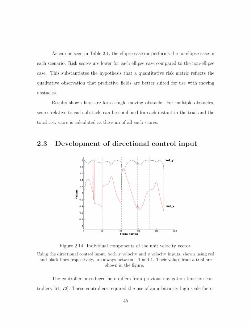
As can be seen in Table 2.1, the ellipse case outperforms the no-ellipse case in

each scenario. Risk scores are lower for each ellipse case compared to the non-ellipse

case. This substantiates the hypothesis that a quantitative risk metric reflects the

qualitative observation that predictive fields are better suited for use with moving

obstacles.

Results shown here are for a single moving obstacle. For multiple obstacles,

scores relative to each obstacle can be combined for each instant in the trial and the

total risk score is calculated as the sum of all such scores.

2.3 Development of directional control input

Figure 2.14: Individual components of the unit velocity vector.

Using the directional control input, both x velocity and y velocity inputs, shown using redand black lines respectively, are always between −1 and 1. Their values from a trial are

shown in the figure.

The controller introduced here differs from previous navigation function con-

trollers [61, 72]. These controllers required the use of an arbitrarily high scale factor

45

Ks in Eq. 2.6) to drive the robot to goal. The resultant system was found to be ex-

tremely gain-sensitive and it was difficult to empirically estimate the scaling required

for the robot to be successfully driven to goal for a particular configuration. Thus,

a modification is made to the control input, driving the robot using the direction of

the navigation gradient rather than the gradient itself. The control input to drive the

robot to q∗ is:

q = u. (2.13)

where u is modified to be

u = −K

(

∂ϕ∂q

)T

∥

∥

∥

∂ϕ∂q

∥

∥

∥+ ǫ

K ∈ R2×2 is a matrix of positive gain values and ǫ is a small positive constant.

Components of the unit control input vector are seen in Figure 2.14. A similar,

normalized control input was also used by Filippidis and Kyriakopoulos [77], citing

the high value of the navigation gain k as a motivating factor.

2.3.1 Stability Analysis

Consider a Lyapunov candidate function, same as the one used by Chen et al.

[72],

V (q) = ϕ(q). (2.14)

First differentiating (2.14) with respect to time and then substituting the right hand

side of the control equation yields

V = ∂ϕ∂q

· q

= −∂ϕ∂q

·K · ( ∂ϕ∂q )

T

‖ ∂ϕ∂q ‖+ǫ

= −f(t)

46

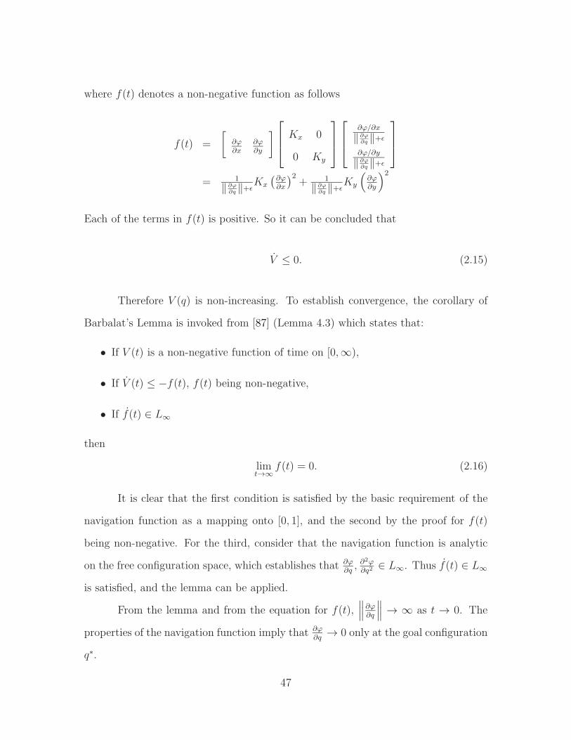
where f(t) denotes a non-negative function as follows

f(t) =

[

∂ϕ∂x

∂ϕ∂y

]

Kx 0

0 Ky

∂ϕ/∂x

‖ ∂ϕ∂q ‖+ǫ

∂ϕ/∂y

‖ ∂ϕ∂q ‖+ǫ

= 1

‖ ∂ϕ∂q ‖+ǫ

Kx

(

∂ϕ∂x

)2+ 1

‖∂ϕ∂q ‖+ǫ

Ky

(

∂ϕ∂y

)2

Each of the terms in f(t) is positive. So it can be concluded that

V ≤ 0. (2.15)

Therefore V (q) is non-increasing. To establish convergence, the corollary of

Barbalat’s Lemma is invoked from [87] (Lemma 4.3) which states that:

• If V (t) is a non-negative function of time on [0,∞),

• If V (t) ≤ −f(t), f(t) being non-negative,

• If f(t) ∈ L∞

then

limt→∞

f(t) = 0. (2.16)

It is clear that the first condition is satisfied by the basic requirement of the

navigation function as a mapping onto [0, 1], and the second by the proof for f(t)

being non-negative. For the third, consider that the navigation function is analytic

on the free configuration space, which establishes that ∂ϕ∂q, ∂

2ϕ∂q2

∈ L∞. Thus f(t) ∈ L∞

is satisfied, and the lemma can be applied.

From the lemma and from the equation for f(t),∥

∥

∥

∂ϕ∂q

∥

∥

∥→ ∞ as t → 0. The

properties of the navigation function imply that ∂ϕ∂q

→ 0 only at the goal configuration

q∗.

47

Hence it is proven that

q(t) → q∗ (2.17)

within a specific workspace.

The control input described in this section uses the gradient of the navigation

function. The gradient vector is normalized to unit magnitude, but its x and y com-

ponents vary according to the direction of the gradient. This unit-length directional

vector is multiplied by the gain K to create a constant magnitude, velocity control,

input to the robot. The control input described here thus solves the problem of high

velocity inputs while demonstrably resulting in convergence to goal.

2.4 Development of workspace generation method

For practical use of predictive fields, two limitations of the original navigation

function method have yet to be addressed:

• Navigation functions only work in circular or star worlds.

• Navigation functions are incompatible with moving goal positions.

These two points are addressed in this section. For our proposed method of workspace

generation, the following reasonable assumptions are made:

• The robot’s sensing range is limited,

• The sensor (e.g. Microsoft Kinect) gathers all information necessary to imple-

ment a predictive fields path planner, and

• The person to be followed is generally within the sensing range of the robot.

48

Figure 2.15: Generation of workspace compatible with navigation functions.

A long, L-shaped hallway is divided into multiple workspaces. Each workspace envelope isshown by the large black circle. Wall lines, in red, are encapsulated using larger circular,red wall obstacles. The lone internal obstacle in this example is shown using a small red

circle. The robot, shown using a small black circle, starts from the bottom of theworkspace and converges to the goal for that workspace, shown using the plus sign.

2.4.1 Workspace representation

Each of the two geometries required for navigation functions, i.e. truly circu-

lar world or start transformed world, is prohibitive for different reasons. Practical

indoor workspaces do not resemble circular worlds, and finding a mapping from a

practical workspace (star-world) to a circular world is non-trivial. These constraints

compel exploring a third option, in which a practical workspace is represented as a

circular world without the complications of a star world transformation. A simplified

representation of a practical workspace makes it possible to use predictive fields in

real-world scenarios.

The work by Tanner et al. [73] includes a ‘union of ellipsoids’ approach, which

is one such attempt at simplified representation. In their work, the non-spherical

robot and obstacles are represented as a combination of smaller ellipsoids, following

which the entire system of ellipsoids is transformed to point obstacles on which the

Rimon-Koditschek formulation is designed to operate. The basis of the idea, i.e.

49

decomposing an object as a union of circular envelopes where necessary, is used here,

without the subsequent deformative transformations to point bodies.

To begin this representation, the workspace envelope for the navigation func-

tion is defined using the limited sensing range of the robot. The area of the hallway

visible to the robot is enveloped by a circular workspace. Segments of the wall which

intersect this sensing envelope are computed. The wall is an obstacle the robot needs

to avoid, hence it is represented as a union of non-overlapping circular obstacles

generated using wall segments from the previous step. The robot and each of the

stationary and moving obstacles are also encompassed by circular envelopes, thus

defining non-wall obstacles for the generated workspace. With this, the workspace

has been defined such that it is fully compatible with the requirements of navigation

functions. All the components of the workspace, inclusing the workspace itself, are

encompassed by circular envelopes. The generated workspace is shown in Fig. 2.15.

2.4.2 Waypoints for moving goal tracking

The setup described previously will work well for a single generated workspace.

But to extend it over the duration of the person following task, it is necessary to

address the navigation function requirement that goal position is not allowed to move

inside a workspace. This constraint renders navigation functions, in their original

form, unusable for person following applications, where the goal is generally moving.

Thus, it is necessary to come up with a description of workspaces which reconciles

this contradiction between the requirements of the motivating application and those

of navigation functions.

To achieve this, the sensing and path planning modules of the system are

decoupled in a specific manner. Since person following is the motivating application

50

Figure 2.16: Generation of leader waypoints as the robot follows the leader.

The entire L-shaped hallway is represented as an union of of circular workspace envelopes(large black circles). The observed leader trajectory is marked by a number of waypoints(plus signs), each of which is the goal position for its workspace. Waypoint generationallows a moving goal (leader) to be tracked across the hallway using the path planner.

Small black circles show obstacles contained within each generated workspace. Note thatone obstacle may be common to multiple workspaces.

for this path planner, the ‘moving goal’ is called the ‘leader’. During initialization,

the first observed position of the leader is set to be the goal position for the first

workspace. This is the first waypoint for the trial.

It is assumed that the sensing module keeps track of the leader even when the

leader moves out of the current path planning workspace. The setup is visualized

as follows. As the robot moves to the goal position in the ith workspace, its sensing

module tracks the leader. On converging to the ith goal, the sensing algorithm has

identified the i+ 1th goal position. Each workspace contains obstacles which become

part of the predictive fields formulation for that workspace. This process continues

until the person stops or the robot is commanded to stop following the leader. A

sample setup, generated waypoints, and obstacles for each workspace are seen in

Figure 2.16. Workspaces are generated so that the predictive fields solution to each

51

workspace is that of robot convergence to a static goal position, shown as a “+” in

the figure. Moving obstacles are represented as solid circles.

This completes the description of workspaces such that the robot can follow

a person without violating any of the constraints of navigation functions, and with-

out requiring geometric transformations for arbitrarily shaped hallways. Simulation

results which demonstrate such a system at work are given in the next section.

52

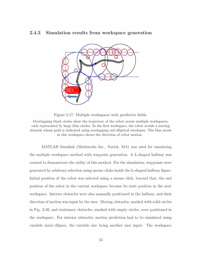
2.4.3 Simulation results from workspace generation

Figure 2.17: Multiple workspaces with predictive fields.

Overlapping black circles show the trajectory of the robot across multiple workspaces,each represented by large blue circles. In the first workspace, the robot avoids a moving

obstacle whose path is indicated using overlapping red elliptical envelopes. The blue arrowin this workspace shows the direction of robot motion.

MATLAB Simulink (Mathworks Inc., Natick, MA) was used for simulating

the multiple workspace method with waypoint generation. A L-shaped hallway was

created to demonstrate the utility of this method. For the simulation, waypoints were

generated by arbitrary selection using mouse clicks inside the L-shaped hallway figure.

Initial position of the robot was selected using a mouse click; beyond that, the end

position of the robot in the current workspace became its start position in the next

workspace. Interior obstacles were also manually positioned in the hallway, and their

direction of motion was input by the user. Moving obstacles, marked with solid circles

in Fig. 2.16, and stationary obstacles, marked with empty circles, were positioned in

the workspace. For interior obstacles, motion prediction had to be simulated using

variable sized ellipses, the variable size being another user input. The workspace

53

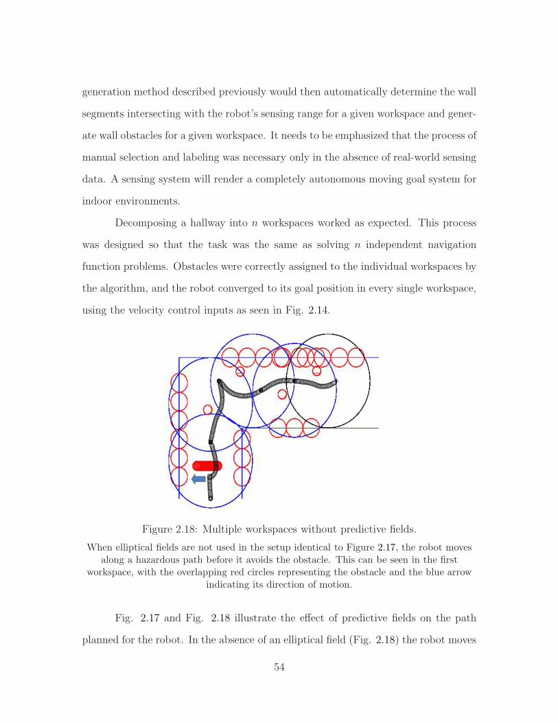
generation method described previously would then automatically determine the wall

segments intersecting with the robot’s sensing range for a given workspace and gener-

ate wall obstacles for a given workspace. It needs to be emphasized that the process of

manual selection and labeling was necessary only in the absence of real-world sensing

data. A sensing system will render a completely autonomous moving goal system for

indoor environments.

Decomposing a hallway into n workspaces worked as expected. This process

was designed so that the task was the same as solving n independent navigation

function problems. Obstacles were correctly assigned to the individual workspaces by

the algorithm, and the robot converged to its goal position in every single workspace,

using the velocity control inputs as seen in Fig. 2.14.

Figure 2.18: Multiple workspaces without predictive fields.

When elliptical fields are not used in the setup identical to Figure 2.17, the robot movesalong a hazardous path before it avoids the obstacle. This can be seen in the first

workspace, with the overlapping red circles representing the obstacle and the blue arrowindicating its direction of motion.

Fig. 2.17 and Fig. 2.18 illustrate the effect of predictive fields on the path

planned for the robot. In the absence of an elliptical field (Fig. 2.18) the robot moves

54

towards the path of the obstacle before the navigation function guides it away from

it. This increases the chances of a collision in uncertain environments, and of moving

along a path which is less optimal temporally or spatially. In contrast, the elliptical

field provides a path in which the robot moves away from the projected obstacle path

much earlier, as seen in Fig. 2.17.

Figure 2.19: Multiple workspaces with stationary obstacles.

When obstacles in multiple workspaces are stationary, the predictive path planningproblem reduces to navigation function path planning. The setup shown here is similar to

Figures 2.17 and 2.18 but for the positions of stationary obstacles.

It can be seen that, for stationary obstacles, the elliptical field is absent and

the predictive formulation reduces to that seen in the classical navigation function

systems [72, 61]. An example of this can be seen in Fig. 2.19.

The use of a direction based controller allows for a very standard gain value

to be used in the setup. The navigation function only has a single gain k which needs

to be tuned; however, this gain is critical to the working of navigation function based

path planners. We found that a gain value between k = 10 and k = 15 in Eq. 2.1 was

adaptable to a wide variety of scenarios in our simulated indoor hallway environment.

The system scale factor Ks, typically a very large gain, was completely eliminated by

55

our choice of controller.

The predictive path planner has thus been developed theoretically, and its

performance has been demonstrated in simulated environments. In the next chapter,

an experimental setup for mobile robot navigation using the predictive fields path

planner is detailed and its results provided.

56

Chapter 3

Experimental verification of

predictive fields path planning

Despite mathematical guarantees of convergence and a global minimum at the

goal, navigation functions have been limited in their direct applicability to experimen-

tal systems. The two principal obstacles in the way have been, (a) the requirement

that practical workspace be represented as star world formulations, and (b) the im-

practicable, high or low magnitude velocity input generated on using the navigation

gradient to drive the robot to goal. In the previous chapter, theoretical modifications

which make it possible for the predictive fields path planner to be used experimen-

tally have been presented. Here, a step by step explanation for an experimental setup

is provided, accompanied by results which demonstrate that predictive fields path

planning meets theoretical expectations and replicates simulation results.

The predictive fields path planner reduces to the classical navigation func-

tion path planner when the obstacles are stationary. Since the representation of the

workspace has been altered to make it more amenable to experiment, this experimen-

tal verification of the navigation function path planner may be one of the first such

57

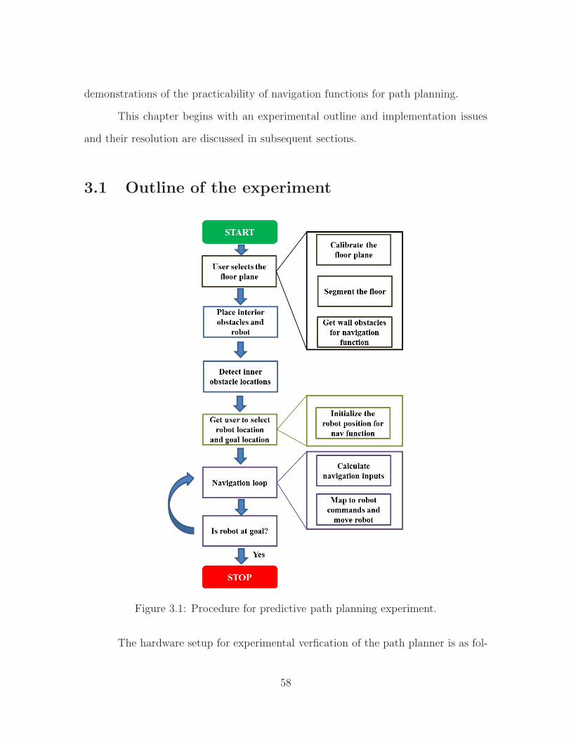
demonstrations of the practicability of navigation functions for path planning.

This chapter begins with an experimental outline and implementation issues

and their resolution are discussed in subsequent sections.

3.1 Outline of the experiment

Figure 3.1: Procedure for predictive path planning experiment.

The hardware setup for experimental verfication of the path planner is as fol-

58

lows. The Kinect RGB-D sensor is mounted about 2.7 meters above the ground, look-

ing down at the floor, which constitutes the robot workspace. An iRobot Roomba is

used as the robot and control commands are issued using its remote control. Switches

on the remote control are activated and deactivated using transistor driven relays.

The remote control is connected to the path planning implementation on the laptop

via a LabJack U3 USB data acquisition device. The Brookstone Rover, controlled by

a mobile app, is programmed to travel along a predefined path as the moving obstacle

in the experiment.

The software setup for the above hardware configuration is as follows. A Mi-

crosoft Visual Studio 10 Solution is created to interface with all the elements of the

system. LabJack software libraries provide access to high-level, C/C++ functions

to control the ports on the device. Blepo, an open source computer vision library,

provides an interface to the Kinect by integrating a number of Microsoft Kinect SDK

function calls. Finally, MATLAB provides a COM interface to all of its functions,

which is set up in the Visual Studio environment. This interface makes it possible to

compute navigation inputs to the robot using MATLAB’s symbolic partial differen-

tiation functions.

During the rest of this chapter, references will be made to two types of ob-

stacles: wall obstacles and interior obstacles. This distinction is necessitated by the

nature of the experimental setup. Experimental trials consist of optional calibration

steps where objects such as the robot and stationary and moving obstacles, have been

removed. Walls in the environment are, however, a constant and non-removable fea-

ture. ‘Internal obstacles’ is thus a reference to all obstacles in the workspace which

are not wall obstacles. Hence the need for terminology to create a distinction between

the two types of obstacles.

The experimental procedure is outlined in Figure 3.1. A trial broadly consists

59

of the following phases:

• Workspace initialization, to identify the floor plane (workspace) and walls.

• Robot and obstacle initialization, to identify starting positions of the robot and

other obstaces in the workspace.

• Automated navigation, in which the path planner issues motion commands to

the robot for it to avoid obstacles and converge to goal.

A trial begins without the robot and internal obstacles in a workspace. Depth

based segmentation is used to identify the robot and obstacles in this workspace. For

this type of segmentation to be used, the floor plane equation needs to be estimated.

Thus, the first step in any trial is to provide the user the option of estimating the floor

plane by selecting an area in the empty workspace. Alternately, since the camera is

mounted at a fixed position, calibration may be performed during the first trial and

its results used for subsequent trials. After the floor plane is estimated, in a workspace

free of internal obstacles and the robot, all points lying outside the floor plane are

considered to belong to wall obstacles. Hence, wall obstacles in the workspace are

determined.

Next, the robot and internal obstacles are moved into the field of view of the

overhead camera. Using depth-based segmentation and image processing operations,

candidate robot and obstacle positions are displayed on the user interface. This gives

the user an opportunity to select the robot location and goal position. After the wall

obstacles and robot position is eliminated from consideration, all remaining obstacles

are labeled by the algorithm as being internal obstacles. As per the requirements

of navigation function path planning, all obstacles and the robot are enveloped by

circles.

60

From this point forward, the path planner dictates the motion of the robot. A

commercially available robot, the Brookstone Rover, is used as the moving obstacle.

It’s path during the trial is preprogrammed using the Brookstone Rover app for the

iOS. An elliptical envelope is constructed around the moving obstacle using principles

outlined in the previous chapter. Color based image processing is used to estimate the

heading of the robot and correct its orientation to the desired heading calculated by

the navigation function. Thus, the ‘Navigation Loop’ component of the experimental

flowchart in Figure 3.1 guides the robot to goal autonomously. Navigation inputs are

calculated using MATLAB’s symbolic differentiation functions.

In the next section, the interface through which navigation inputs are commu-

nicated to the robot is discussed. In sections subsequent to it, the implementation

algorithms to successfully complete an experimental trial are outlined.

3.2 Controlling the robot

Control commands are issued to the robot based on navigation function inputs.

The iRobot Roomba Create is used in this experiment. The possibility of using the

Create’s programmable serial interface to download the navgiation algorithm to it

was considered. The problem with this option is that only the sensors onboard the

Roomba can be used for the motion planner. This condition is prohibitive for the

predictive fields experiment, since RGB-D cues are being used to provide workspace

information to the path planning module. The alternative to downloading a program

to the Roomba is then to interface with the robot remotely and issue commands from

the program running on the user’s laptop.

Such a remote interface is created by using a commercially available Roomba

Remote Control to control the robot. The Roomba remote control provides access

61

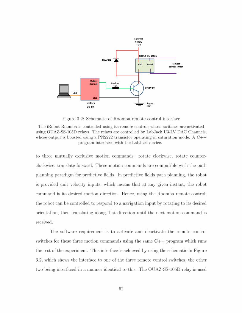
Figure 3.2: Schematic of Roomba remote control interface

The iRobot Roomba is controlled using its remote control, whose switches are activatedusing OUAZ-SS-105D relays. The relays are controlled by LabJack U3-LV DAC Channels,whose output is boosted using a PN2222 transistor operating in saturation mode. A C++

program interfaces with the LabJack device.

to three mutually exclusive motion commands: rotate clockwise, rotate counter-

clockwise, translate forward. These motion commands are compatible with the path

planning paradigm for predictive fields. In predictive fields path planning, the robot

is provided unit velocity inputs, which means that at any given instant, the robot

command is its desired motion direction. Hence, using the Roomba remote control,

the robot can be controlled to respond to a navigation input by rotating to its desired

orientation, then translating along that direction until the next motion command is

received.

The software requirement is to activate and deactivate the remote control

switches for these three motion commands using the same C++ program which runs

the rest of the experiment. This interface is achieved by using the schematic in Figure

3.2, which shows the interface to one of the three remote control switches, the other

two being interfaced in a manner identical to this. The OUAZ-SS-105D relay is used

62

to activate and deactivate the switches. This relay is switched on and off by setting

up a PN 2222 NPN transistor to work as a switch. The switching (base) input to this

switch is provided by commands from the LabJack U3-LV data acquisition device.

The U3 has two DAC channels to interface with two of the three remote control

inputs. One of the Digital I/O ports is programmed to output the switching signal

to the third remote control input. LabJack U3 has software examples to show how it

can be controlled by a Visual Studio 6.0 program. With minimal modifications, the

same setup was used for the Visual Studio 10 Solution which ran this experiment.

3.3 Workspace and wall obstacle representation

Workspace and wall obstacle representation comprises of the following com-

ponents:

• Identification of the plane of the workspace

• Identification of wall obstacles using segmentation

Establishing the workspace plane is useful for the idenfication of the robot and

internal obstacles. Further, knowing the extent of the workspace is required for iden-

tification of the workspace envelope, which contributes to one of the repulsive terms

in the navigation function. Walls are static obstacles which are also represented in

the navigation function using repulsive terms. Moreover, they are also immovable

objects in the workspace. Hence, they need to be identified, segmented, and repre-

sented at the same time as the plane of the workspace. Once the workspace and wall

positions have been deduced, the robot and internal obstacles are introduced into

the workspace. The knowledge of the floor plane equation is used to segment these

63

objects from the background of the workspace plane using depth. The details of this

initialization process are explained in this section.

3.3.1 Floor plane estimation

(a) Floor area is selected by the user. (b) Corresponding area in the color image.

Figure 3.3: Selection of points for estimation of floor plane equation.

To estimate the floor plane equation, the user selects a rectangular area in the depthimage. Its corresponding region in the color image is shown using a red rectangle. All

points inside the area are used in formulating the least squares solution to the floor planeequation.

The Kinect RGB-D sensor gives access to depth data, which in turn can be

converted to a 3D coordinate system using the camera calibration matrix specific

to this sensor. Assuming that the workspace is planar, the equation of the plane

can be estimated using a set of labeled floor points. Any point in the depth image

not satisfying the floor plane equation can thus be labeled as a point on a potential

obstacle. This labeling serves as the initial step towards detection of the robot and

other obstacles.

Floor plane estimation begins with a workspace without either the robot or

one of the interior obstacles in the field of view. The estimation step allows the user

to select an area in the color or depth image, as seen in Figure 3.3. All points in this

64

area are considered for floor plane estimation. The floor plane can be represented by

the equation

z = ax+ by + c (3.1)

where the triplet (x, y, z) represents 3D coordinates of a point (in meters), and a,b,c

are floor plane parameters. Floor plane parameters are estimated using a least squares

formulation [88],

Af = B (3.2)

where

A =

∑Ni=1 x

2i

∑Ni=1 xi · yi

∑Ni=1 xi

∑Ni=1 xi · yi

∑Ni=1 y

2i

∑Ni=1 yi

∑Ni=1 xi

∑Ni=1 yi N

B =

∑Ni=1 xi · zi

∑Ni=1 yi · zi

∑Ni=1 zi

In the above formulation, N points are used for the least squares fit, [ xi yi zi ]

being the 3D coordinates of each point. The solution of the least squares equation

is the vector f , the elements of which are the desired coefficients of the floor plane

equation, i.e.

f =

a

b

c

65

Figure 3.4: Labeling wall obstacle lines.

For a fixed setup, wall obstacles are defined using lines labeled by the user. The userselects two points in the color image, and the y coordinates of these points are used tocreate horizontal red lines spanning the image. Evenly spaced wall obstacles are created

given these user-defined lines.

3.3.2 Labeling wall obstacles

Identifying the position of walls in the workspace is another initialization pro-

cedure. Since wall locations are assumed to be fixed for the experimental setup, this

is a single time labeling process which need not be repeated for each trial. The user

is asked to label two points [xtop, ytop] and [xbottom, ybottom] in the depth image, to

approximate the y coordinates of the wall lines at the top and bottom of the image

respectively. The lines y = ytop and y = ybottom, shown in Figure 3.4, are then used

to set up wall obstacles. In keeping with the requirements of the navigation function

setup, these line segments are divided into non-overlapping circular wall obstacles.

3.3.3 Depth based segmentation

Depth based segmentation, during initialization and over the course of the

trial, serves as the input to the tracking algorithm for the positions of internal ob-

stacles, and the robot. Wall obstacle locations, as determined by the user labeling in

66

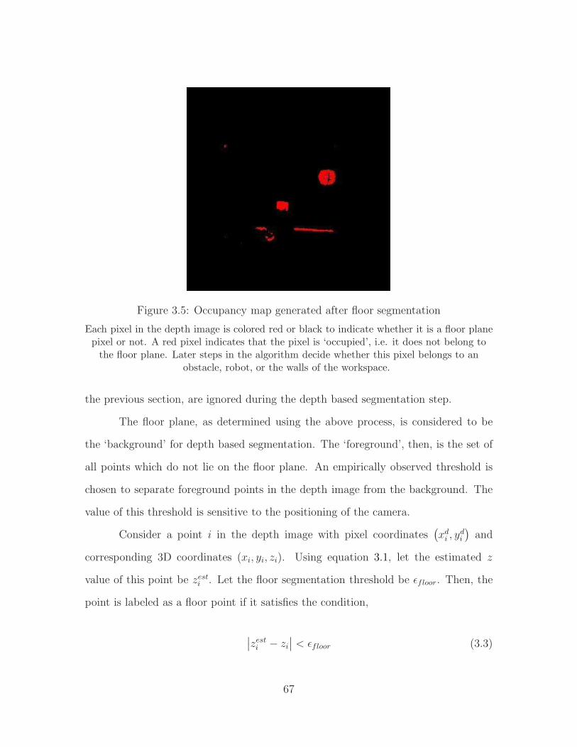
Figure 3.5: Occupancy map generated after floor segmentation

Each pixel in the depth image is colored red or black to indicate whether it is a floor planepixel or not. A red pixel indicates that the pixel is ‘occupied’, i.e. it does not belong tothe floor plane. Later steps in the algorithm decide whether this pixel belongs to an

obstacle, robot, or the walls of the workspace.

the previous section, are ignored during the depth based segmentation step.

The floor plane, as determined using the above process, is considered to be

the ‘background’ for depth based segmentation. The ‘foreground’, then, is the set of

all points which do not lie on the floor plane. An empirically observed threshold is

chosen to separate foreground points in the depth image from the background. The

value of this threshold is sensitive to the positioning of the camera.

Consider a point i in the depth image with pixel coordinates(

xdi , y

di

)

and

corresponding 3D coordinates (xi, yi, zi). Using equation 3.1, let the estimated z

value of this point be zesti . Let the floor segmentation threshold be ǫfloor. Then, the

point is labeled as a floor point if it satisfies the condition,

∣

∣zesti − zi∣

∣ < ǫfloor (3.3)

67

Figure 3.6: Morphological processing of occupancy image

The raw data from Figure 3.5 is processed to generate this binary image which is used todetect robot and inner obstacle positions. Wall pixels are discarded, and the remaining

pixels are operated upon by morphological operators. This gives foreground regions (whiteblobs) which can be processed as robot or internal obstacle candidates.

For an overhead camera view, it was found that a threshold of ǫfloor = 0.07 was

required to discriminate between the floor plane and other elements of the workspace.

The outcome of this segmentation process is an occupancy map as seen in

Figure 3.5, where the red pixels are non-floor points. Since the floor segmentation

threshold is chosen empirically, some noisy foreground pixels are likely to appear

in an occupancy map. To filter out the noise and retain genuine foreground areas,

morphological operations such as erosion and dilation are applied to the occupancy

map. The outcome of morphology, as seen in Figure 3.6 is a clean binary image in

which most of the noise has been removed.

68

3.4 Robot and internal obstacle tracking

After wall obstacles have been identified and the floor has been segmented,

the positions of the robot and internal obstacles need to be updated over time. Initial

positions of these objects is set using user input. After initialization, the trial enters

the fully autonomous Navigation Loop phase as shown in Figure 3.1, and ‘tracking

by detection’ is used to match detections to determine the current position of these

objects. In addition to tracking, robot heading needs to be estimated for each iteration

of the trial. This is done using color segmentation. Each step of the tracking process

is explained in this section.

3.4.1 Tracker initialization

Morphological processing (Figure 3.6) results in blobs which are processed fur-

ther using connected components. Areas which are too small or too large (determined

by expected size of robot and obstacles in the occupancy image) are filtered out. Areas

which belong to wall obstacles have already been filtered out during pre-processing

before morphology.

Thus, the remaining connected regions are either internal obstacles or the

robot. The center and bounding box of each region provides enough information to

encapsulate them using circles, as required by navigation functions. User input is

now required to establish which of these candidates is the robot. The selected robot

position in the occupancy map in frame 0 is [xrobot0 , yrobot0 ]. This is represented by

a white circle around the object, as seen in Figure 3.7. Every other object is now

classified as an internal obstacle. The ith internal obstacle at frame 0 is represented

using occupancy map coordinates [xi0, y

i0]. A blue circle in Figure 3.7 denotes internal

obstacles.

69

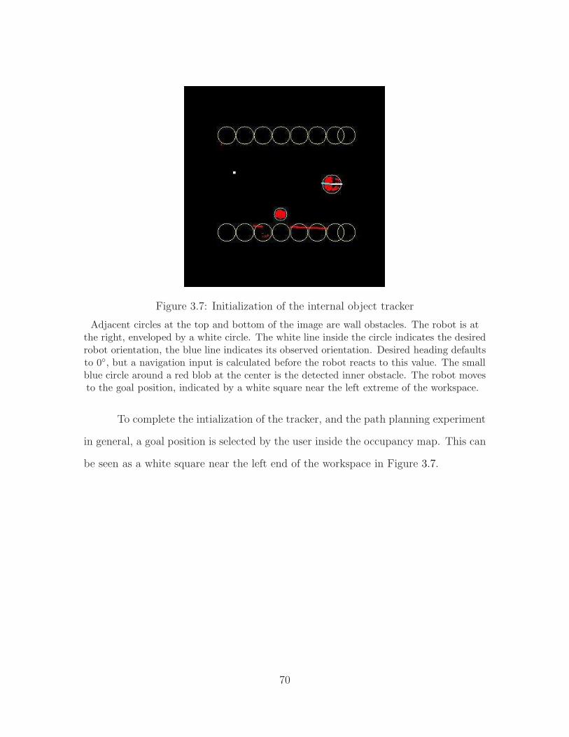
Figure 3.7: Initialization of the internal object tracker

Adjacent circles at the top and bottom of the image are wall obstacles. The robot is atthe right, enveloped by a white circle. The white line inside the circle indicates the desiredrobot orientation, the blue line indicates its observed orientation. Desired heading defaultsto 0◦, but a navigation input is calculated before the robot reacts to this value. The smallblue circle around a red blob at the center is the detected inner obstacle. The robot movesto the goal position, indicated by a white square near the left extreme of the workspace.

To complete the intialization of the tracker, and the path planning experiment

in general, a goal position is selected by the user inside the occupancy map. This can

be seen as a white square near the left end of the workspace in Figure 3.7.

70

3.4.2 Robot and obstacle tracking

Figure 3.8: Prediction of object position and matching to detected blob

Internal object detections, using depth based segmentation (Section 3.3.3), are

matched to get the tracker output. Figure 3.8 is a representation of the object tracking

process. The first step in matching detections is predicting the current positions of

objects based on their motion history. A simple, linear prediction model is used

to predict object locations for the current iteration n, although more sophisticated

algorithms such as Kalman filters may conceivably be used for the same purpose.

For an object located at [xn−1, yn−1] during iteration n− 1 and at [xn−2, yn−2] during

iteration n−2, the predicted position [xn+1, yn] during the current iteration n is given

by

∆x = xn−1 − xn−2

∆y = yn−1 − yn−2

xn+1 = xn−1 +∆x

yn+1 = yn−1 +∆y

71

Each detected internal object is projected to an expected current position in this

manner. These expected positions are then matched to blob detections from depth

segmentation, and each object gets assigned the blob closest to its predicted position.

The value of computing expected positions for the robot and each internal obstacles is

in disambiguating blobs which are close to each other. Such a situation is commonly

observed when the robot is moving past an obstacle.

3.4.3 Robot heading estimation

Figure 3.9: Calibration of hue and saturation values to identify markers

Front and back marker Hue-Saturation values are calibrated using user input. The usermarks one point each on the front and back markers in the hue image (left) and saturation

image (right).

The robot is issued directional navigation commands in the form of heading

inputs in degrees. Following a navigation command, the robot heading is corrected to

the desired heading, and the robot translates along this heading until the next naviga-

tion command is available. Correcting robot orientation requires accurate feedback,

which makes heading estimation an important module in the path planning imple-

mentation.

The position of the robot and a bounding box for it in terms of occupancy

72

Figure 3.10: Output of heading estimation

Given the hue-saturation calibration from Figure 3.9, robot heading can be detected. Thered dot on the front (orange) pad indicates the estimated center of the front marker, andthe green dot on the back (blue) pad indicates the estimated center of the back marker.

map coordinates is available after tracking. To distinguish the front and back of

the robot, colored markers are placed on the top of the robot. Marker color values

are calibrated in terms of Hue and Saturation from the HSV colorspace. Conversion

from RGB to HSV provides access to a color space in which the illumination variant

component (Value) is separated and hence color detection is more robust to effects

such as shadows. For a fixed, indoor setup, front and back marker calibration needs

to be done just a single time. It is done by allowing the user to click somewhere

on the front and back marker in the hue and saturation images, as seen in Figure

3.9. A tolerance around the values at the selected image pixels creates a minimum

and maximum threshold for hue ([Hfrontmin , Hfront

max ] and [Hbackmin , H

backmax ] ) and saturation

([Sfrontmin , Sfront

max ] and [Sbackmin , S

backmax]). The range of values for hue and saturation is

[0 . . . 1].

During a trial, positions of these markers are estimated by identifying color

image pixels satisfying calibrated color values for the front and back marker. Search

for these matching color pixels is restricted to the robot bounding box. Thus, for

73

a point with pixel coordinates [xi, yi], with hue and sat values H[xi,yi] and S[xi,yi]

respectively, if

Hfrontmin < H[xi,yi] < Hfront

max , and

Sfrontmin < S[xi,yi] < Sfront

max

then it belongs to the front marker, and if

Hbackmin < H[xi,yi] < Hback

max , and

Sbackmin < S[xi,yi] < Sback

max

then it belongs to the back marker.

The centroids of the front and back markers are calculated, and the orientation

of the line connecting them gives the heading of the robot for the current iteration.

An example of this estimation output is seen in Figure 3.10. The red marker in the

figure shows the estimated location of centroid of the front marker. The green marker

is the estimated location of the centroid of the back marker.

When obstacles are being tracked, the predictive fields algorithm dictates that

their motion be represented using ellipses as explained in Section 2.2. Ellipse gener-

ation for obstacles during run-time is explained in the next section.

74

3.4.4 Obstacle ellipse generation

Figure 3.11: Generation of obstacle ellipse

The four images on the left show different frames leading to ellipse generation. Thecharacteristic features of each image are explained in Figure 3.7. The obstacle, at the

center of each image and enveloped by a blue circle, moves downward. As moreinformation about the obstacle motion becomes available, its ellipse can be generated.

The generated ellipse can be seen in the two MATLAB plots to the right. The red circleshows the actual position of the obstacle, and the black circle shows its projected position

inside the elliptical envelope. When not enough information about obstacle motion isavailable, the red and black circles overlap, as seen in the top image.

The path planner proposed in the previous chapter can be tested experimen-

tally only after obstacle motion is represented in the form of an elliptical field. Ob-

75

stacle ellipses are generated based on the knowledge of the direction vector of the

obstacle. For a proof of concept experiment, the following assumptions are made for

ellipse generation:

• The obstacle moves along a straight line.

• The obstacle moves with a constant velocity.

This type of obstacle motion can then be encapsulated using an ellipse at a fixed

orientation and of a fixed size. These assumptions can be easily relaxed for a imple-

mentation of a practical system which uses predictive fields path planning.

The orientation vector for an obstacle is generated after observing its positional

variation over a few iterations of the trial. If the obstacle has displaced sufficiently

from its initial position, it is considered to be a moving obstacle and an ellipse is

generated for it. Figure 3.11 shows this process. Occupancy maps on the left of the

figure show tracked positions of the robot and internal obstacles over a few iterations

at the beginning of the trial. The figures to the right are the representation of this

data in a form required by navigation functions, i.e. the entire workspace and objects

in it are assigned circular envelopes. As the position of the obstacle changes over a

few iterations of the trial, there is enough displacement to label it a ‘moving obstacle’

and assign an ellipse to it. The first frame at the top left of the figure is the beginning

of the trial, the last frame at the bottom left is the iteration where obstacle ellipse is

generated. The top right and bottom right representations correspond to these two

iterations.

For the experiment, the moving obstacle was a Brookstone Rover robot. This

robot can be controlled by a mobile phone app and one of the possible control modes

is to record and replay a sequence of motions. This mode allowed the moving obstacle

to move along a predefined linear trajectory during the trial.

76

The setup for an experiment is thus completed, and results from the trials are

highlighted in the next section.

3.5 Results

The experimental trials described here were carried out in a fixed workspace,

hence obviating the need for repeated calibrations. As seen in the following sections,

results corroborated the findings of simulated data regarding the efficacy of predictive

fields path planner in dynamic environments.

3.5.1 Parameter settings and test configurations

The system was calibrated once and the same settings were used for all trials.

Floor plane parameters from Eq. (3.1) were: a = 0.02, b = 0.04, and c = 2.39, with a

floor plane segmentation threshold from Eq. (3.3) of ǫfloor = 0.07. Color thresholds

for front and back marker detection (in the range [0 . . . 1] for robot heading estimation

were:

Hfrontmin = 0

Hfrontmax = 0.16

Hbackmin = 0.5

Hbackmax = 0.75

Sfrontmin = 0.27

Sfrontmax = 0.47

Sbackmin = 0.31

Sbackmax = 0.54

There are two tuning paramters for the path planner. Of these, the most important

is the value of the navigation gain k. Based on data from simulations, the tuned

77

Figure 3.12: Convergence to goal with no obstacles

Robot navigation to goal with no internal obstacles, as seen using workspace image to theleft and color image to the right. The workspace image at the top shows initial position ofthe system. The bottom image shows the final position of the system, with the trail ofyellow dots showing various intermediate positions occupied by the robot on its way to

goal.

value of this gain was k = 15. The 3D values observed by the Kinect (in mm) were

scaled to approximately the range used for simulating the path planner. This scaling

resulted in the simulation k value of 15 working perfectly for all experimental trials.

Because of the procedure of the experiment, it was found that the translational

resolution of robot motion was not adequate for the robot to converge exactly to

goal. In early trials, this led to the robot moving around its desired goal position.

This being a limitation of the robot used, an arbitrary stopping distance of 5cm was

78

introduced in the algorithm. This meant that the trial would be terminated as soon

as the distance between the robot and the goal position decreased below the stopping

distance.

To demonstrate the completeness of the path planning experimental setup, re-

sults from different configurations, in an increasing order of complexity, are presented

in this section. The test configurations are as follows:

• Convergence to goal with no internal obstacle

• Convergence to goal with a single internal obstacle

• Convergence to goal with two internal obstacles

• Two examples of convergence to goal with a moving obstacle, no elliptical fields

• Two examples of convergence to goal with a moving obstacle using elliptical

fields

Results are presented as a collage of two images: the color image from the Kinect

with the robot bounding box and front and back marker centroids overlaid, and

occupancy map with the robot and obstacles encapsulated with circular envelopes.

In all cases, the goal position is marked using a white square. Manual labeling on

every nth iteration is used to show the robot path over the trial. This path is shown

as a sequence of yellow squares. In the occupancy map, the robot has two additional

lines overlaid on it. The white line shows the desired orientation of the robot, whereas

the blue line shows the estimated orientation of the robot. Rotation commands are

issued to correct this error before translating the robot.

The first case presented is the most basic: robot converging to the goal in

the absence of internal obstacles. Wall obstacles are considered permanent to the

79

workspace and hence, as discussed earlier, a distinction is made between them and

removable obstacles, which are labeled as being internal obstacles. Figure 3.12 shows

the navigation output with zero internal obstacles. Workspace radius, denoted in

the path planner configuration as ro0 is set to an arbitrary value large enough to

encompass the entire field of view of the Kinect. As seen in the figure, robot converges

to goal following nearly a straight line path, as may be expected for such a test case.

80

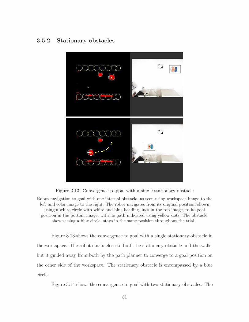
3.5.2 Stationary obstacles

Figure 3.13: Convergence to goal with a single stationary obstacle

Robot navigation to goal with one internal obstacle, as seen using workspace image to theleft and color image to the right. The robot navigates from its original position, shownusing a white circle with white and blue heading lines in the top image, to its goal

position in the bottom image, with its path indicated using yellow dots. The obstacle,shown using a blue circle, stays in the same position throughout the trial.

Figure 3.13 shows the convergence to goal with a single stationary obstacle in

the workspace. The robot starts close to both the stationary obstacle and the walls,

but it guided away from both by the path planner to converge to a goal position on

the other side of the workspace. The stationary obstacle is encompassed by a blue

circle.

Figure 3.14 shows the convergence to goal with two stationary obstacles. The

81

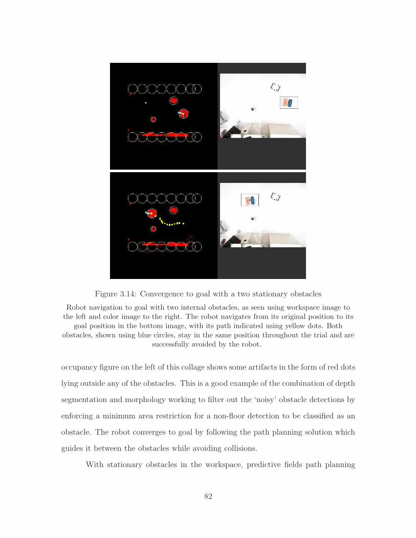
Figure 3.14: Convergence to goal with a two stationary obstacles

Robot navigation to goal with two internal obstacles, as seen using workspace image tothe left and color image to the right. The robot navigates from its original position to its

goal position in the bottom image, with its path indicated using yellow dots. Bothobstacles, shown using blue circles, stay in the same position throughout the trial and are

successfully avoided by the robot.

occupancy figure on the left of this collage shows some artifacts in the form of red dots

lying outside any of the obstacles. This is a good example of the combination of depth

segmentation and morphology working to filter out the ‘noisy’ obstacle detections by

enforcing a minimum area restriction for a non-floor detection to be classified as an

obstacle. The robot converges to goal by following the path planning solution which

guides it between the obstacles while avoiding collisions.

With stationary obstacles in the workspace, predictive fields path planning

82

reduces to the standard form of the navigation function path planner. Hence, all test

cases with stationary obstacles are also examples of the classical navigation function

path planner at work.

83

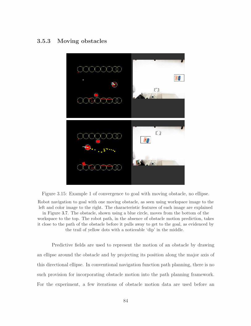
3.5.3 Moving obstacles

Figure 3.15: Example 1 of convergence to goal with moving obstacle, no ellipse.

Robot navigation to goal with one moving obstacle, as seen using workspace image to theleft and color image to the right. The characteristic features of each image are explainedin Figure 3.7. The obstacle, shown using a blue circle, moves from the bottom of the

workspace to the top. The robot path, in the absence of obstacle motion prediction, takesit close to the path of the obstacle before it pulls away to get to the goal, as evidenced by

the trail of yellow dots with a noticeable ‘dip’ in the middle.

Predictive fields are used to represent the motion of an obstacle by drawing

an ellipse around the obstacle and by projecting its position along the major axis of

this directional ellipse. In conventional navigation function path planning, there is no

such provision for incorporating obstacle motion into the path planning framework.

For the experiment, a few iterations of obstacle motion data are used before an

84

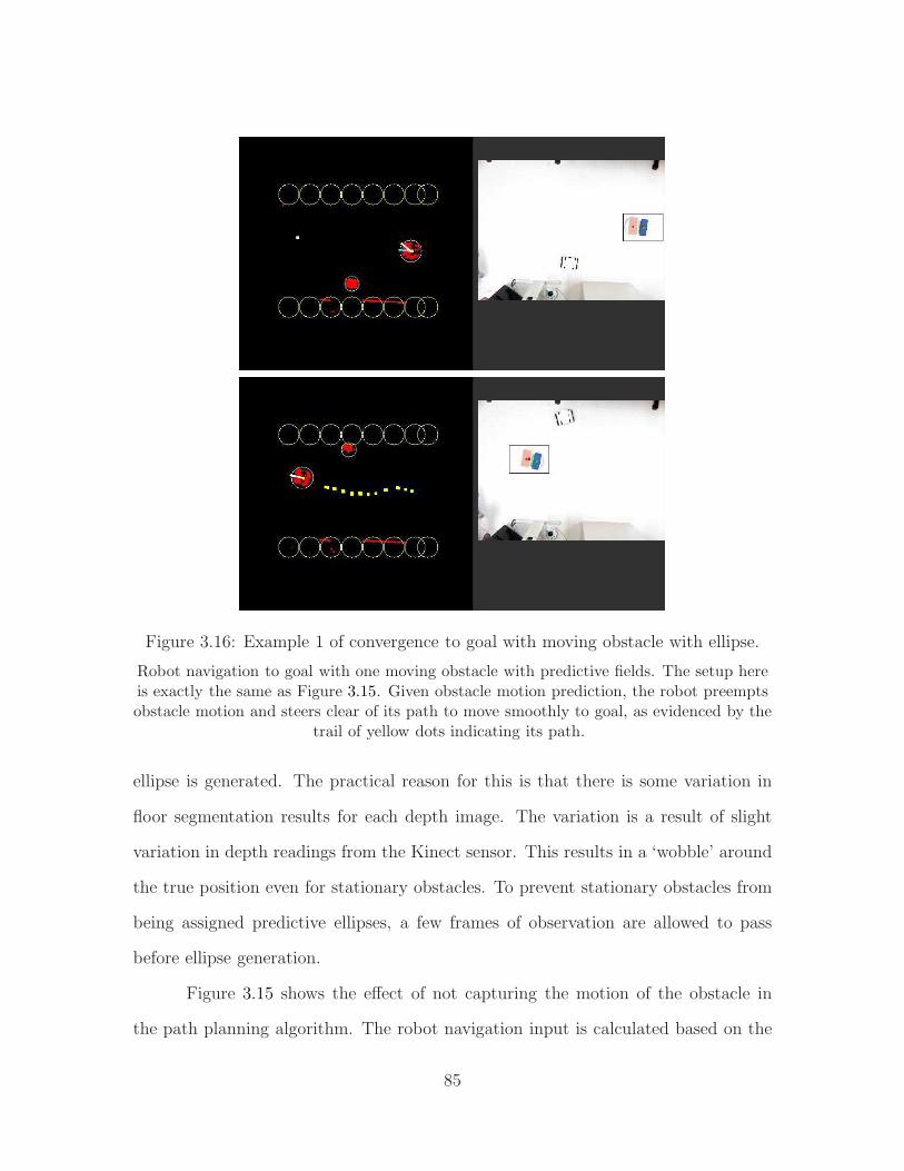
Figure 3.16: Example 1 of convergence to goal with moving obstacle with ellipse.

Robot navigation to goal with one moving obstacle with predictive fields. The setup hereis exactly the same as Figure 3.15. Given obstacle motion prediction, the robot preemptsobstacle motion and steers clear of its path to move smoothly to goal, as evidenced by the

trail of yellow dots indicating its path.

ellipse is generated. The practical reason for this is that there is some variation in

floor segmentation results for each depth image. The variation is a result of slight

variation in depth readings from the Kinect sensor. This results in a ‘wobble’ around

the true position even for stationary obstacles. To prevent stationary obstacles from

being assigned predictive ellipses, a few frames of observation are allowed to pass

before ellipse generation.

Figure 3.15 shows the effect of not capturing the motion of the obstacle in

the path planning algorithm. The robot navigation input is calculated based on the

85

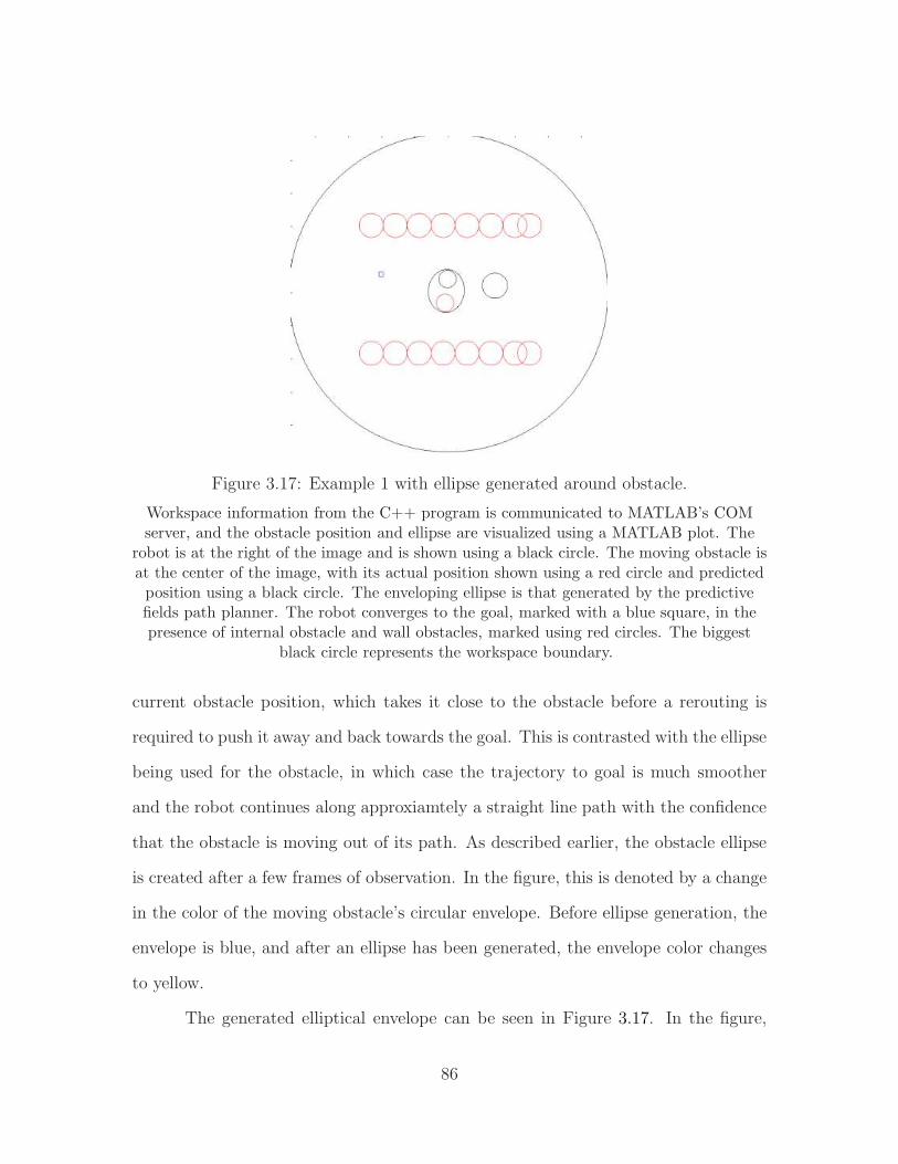
Figure 3.17: Example 1 with ellipse generated around obstacle.

Workspace information from the C++ program is communicated to MATLAB’s COMserver, and the obstacle position and ellipse are visualized using a MATLAB plot. The

robot is at the right of the image and is shown using a black circle. The moving obstacle isat the center of the image, with its actual position shown using a red circle and predictedposition using a black circle. The enveloping ellipse is that generated by the predictivefields path planner. The robot converges to the goal, marked with a blue square, in thepresence of internal obstacle and wall obstacles, marked using red circles. The biggest

black circle represents the workspace boundary.

current obstacle position, which takes it close to the obstacle before a rerouting is

required to push it away and back towards the goal. This is contrasted with the ellipse

being used for the obstacle, in which case the trajectory to goal is much smoother

and the robot continues along approxiamtely a straight line path with the confidence

that the obstacle is moving out of its path. As described earlier, the obstacle ellipse

is created after a few frames of observation. In the figure, this is denoted by a change

in the color of the moving obstacle’s circular envelope. Before ellipse generation, the

envelope is blue, and after an ellipse has been generated, the envelope color changes

to yellow.

The generated elliptical envelope can be seen in Figure 3.17. In the figure,

86

actual position of the obstacle is represented by a red circle, whereas its predicted po-

sition is represented using a black circle. The black circle is the position for which the

repulsive term for navigation is calculated when predictive fields are used. Without

the use of predictive fields, the red circle is used for calculating this term.

87

Figure 3.18: Example 1: Comparing robot positions with and without use of ellipse

When elliptical information is not used, the robot is at a greater risk of moving close tocollision with the obstacle. The top image shows an hazardous robot position without theuse of elliptical information. The robot path, shown using a trail of yellow dots, comes

very close to the obstacle, enveloped by a blue circle. A big heading correction, shown bythe white ‘desired heading’ line is needed to steer the robot away from harm. As opposed

to this, the use of elliptical fields in the lower image keeps the robot away from theobstacle’s projected position.

Not only does the use of elliptical fields make for more efficient navigation, but

also pushes the robot close to colliding with the obstacle. This situation is avoided

using the elliptical position field shown in Figure 3.16. The effect of the robot being

pushed too close to the obstacle can be seen in Figure 3.18. It can be seen that, at

approximately the same position of the obstacle, the robot guided by predictive fields

(bottom image in the collage) is comfortably away from the obstacle when compared

88

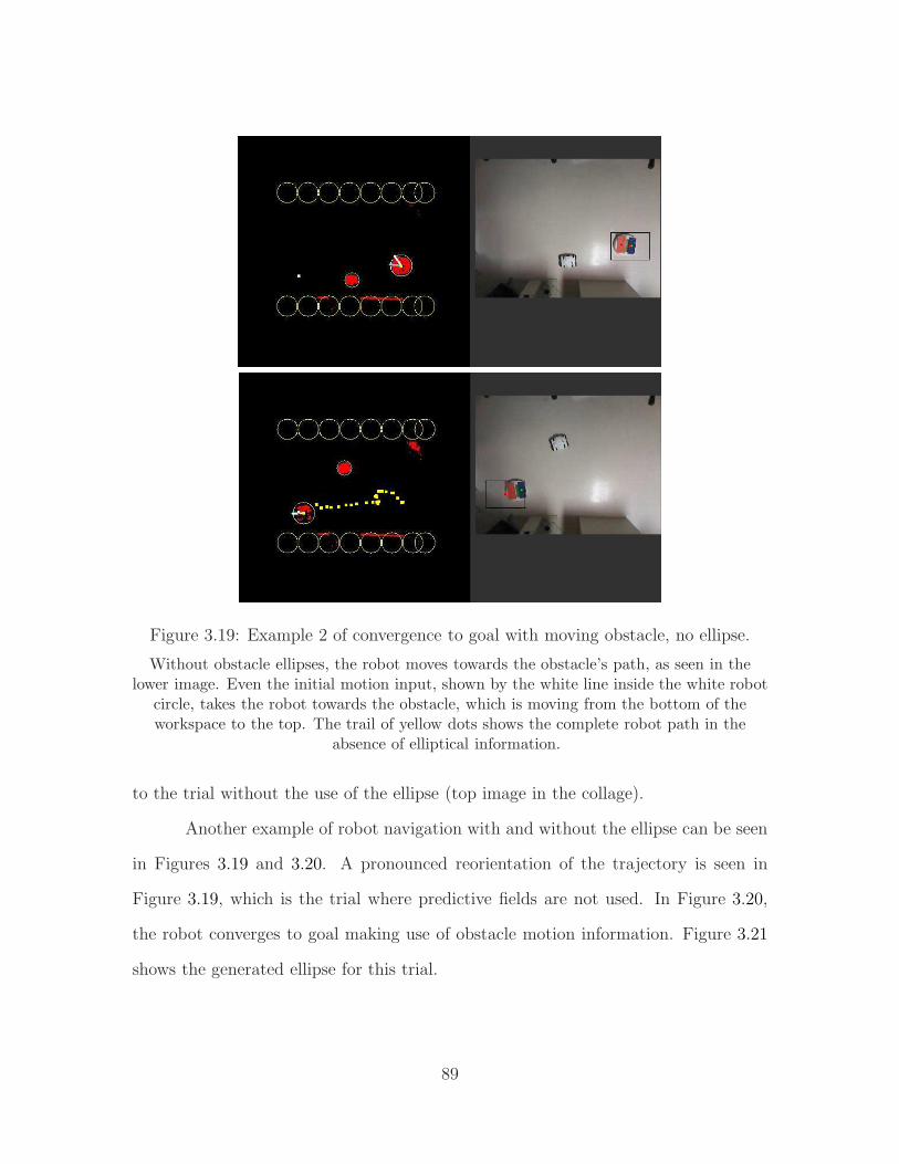
Figure 3.19: Example 2 of convergence to goal with moving obstacle, no ellipse.

Without obstacle ellipses, the robot moves towards the obstacle’s path, as seen in thelower image. Even the initial motion input, shown by the white line inside the white robot

circle, takes the robot towards the obstacle, which is moving from the bottom of theworkspace to the top. The trail of yellow dots shows the complete robot path in the

absence of elliptical information.

to the trial without the use of the ellipse (top image in the collage).

Another example of robot navigation with and without the ellipse can be seen

in Figures 3.19 and 3.20. A pronounced reorientation of the trajectory is seen in

Figure 3.19, which is the trial where predictive fields are not used. In Figure 3.20,

the robot converges to goal making use of obstacle motion information. Figure 3.21

shows the generated ellipse for this trial.

89

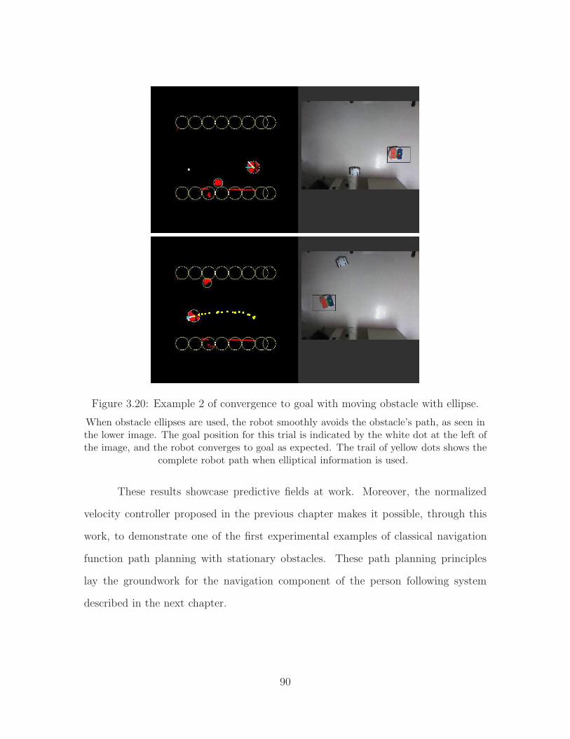
Figure 3.20: Example 2 of convergence to goal with moving obstacle with ellipse.

When obstacle ellipses are used, the robot smoothly avoids the obstacle’s path, as seen inthe lower image. The goal position for this trial is indicated by the white dot at the left ofthe image, and the robot converges to goal as expected. The trail of yellow dots shows the

complete robot path when elliptical information is used.

These results showcase predictive fields at work. Moreover, the normalized

velocity controller proposed in the previous chapter makes it possible, through this

work, to demonstrate one of the first experimental examples of classical navigation

function path planning with stationary obstacles. These path planning principles

lay the groundwork for the navigation component of the person following system

described in the next chapter.

90

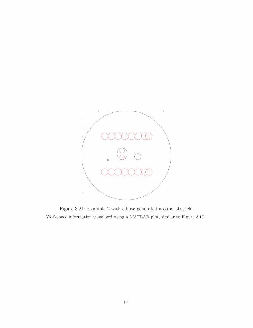
Figure 3.21: Example 2 with ellipse generated around obstacle.

Workspace information visualized using a MATLAB plot, similar to Figure 3.17.

91

Chapter 4

Person following in indoor

environments

The person following system, which is the motivating application for the de-

velopment of the path planner, is described in detail in this chapter. The scope of

the person follower is restricted to common indoor environments such as hallways.

Such a restriction may be imposed without making substantial compromises on the

applicability of this person following system. For example, warehouse robots, medical

robot assistants, and museum guide robots are all service robots which are expected

to function in such environments.

In the initial sections of this chapter, the broad problem of ‘person following’

is discussed in greater detail. The robotic follower is supposed to interact with and

serve a human leader in some capacity. Hence, human involvement is at the center

of a person following system, and a leader-centric classification system is proposed.

To be able to follow a leader around a practical environment, the follower should

avoid confusion between its leader and other people in the scene. To address this re-

quirement, a descriptor based leader identification method is proposed and its results

92

demonstrated.

A robotic follower should be able to find its way to the leader in order to

overcome occlusions, and it should be able to avoid obstacles in its path. Both these

capabilities can only be built into the robotic system when the robot can localize

itself in the environment. This person follower application assumes that the leader

is within a reasonable proximity to the robot, and a comprehensive SLAM system is

not required for such a task. A local map generation technique using 3D data from

depth maps is proposed.

With the ability to localize itself being provided by the mapping subsystem, the

actual task of navigation and obstacle avoidance is demonstrated using the predictive

path planning method developed in previous chapters.

A Pioneer P3-AT mobile robot, with a software interface provided by Aria

libraries, is used for the system prototype. A tripod mounted Kinect is used as the

forward-looking RGB-D sensor for the robot.

4.1 A classification system for person following

4.1.1 System requirements for person followers

The functions of person following robots were first clearly outlined in the work

of Yoshimi et al. [16]. Specifically, they identified that the person following robot

should:

• Initialize to the leader

• Follow the leader at his/her pace

• Avoid obstacles

93

• Resume contact with the leader after occlusions

These tasks capture the system requirements of a person follower quite concisely.

Subsequent work on person following, for example [41, 19, 34, 20], either consciously

or otherwise has tended to design the system based on these person following objec-

tives. The systemic implementation described in this chapter fits in neatly with these

objectives.

These tasks are robot-specific requirements, i.e. an outline of what the robot

is supposed to do when following a person. It is equally important to consider the

role of the person leading the robot in such an application. In service robotics, the

person is interested in having a robotic companion follow him or her around and there

is no intention of putting the robot off the trail of the leader. However, a populated

indoor environment poses unique challenges to the success of such an human-robot

interaction. There are many situations where the leader, despite fully intending to

stay within sight of the follower robot, is likely to be outside the direct line of sight

of the robot’s sensor.

This raises a subtle yet relevant question in terms of human robot interaction

- how much is the leader required to cooperate with the robot and comply with the

various limitations of the robotic follower? In future studies, it will be desirable to

establish a metric for the quality of robotic followers. It is proposed that a categoriza-

tion of robotic person followers based on the degree of cooperation expected from the

leader will be a useful parameter for such a metric. The robotic person follower could

be assigned a ‘level’ of sophistication based on the degree of cooperation expected

from its leader. Each level can still accommodate a complex range of challenges for

the robotic system, e.g. mapping, tracking, depth estimation.

94

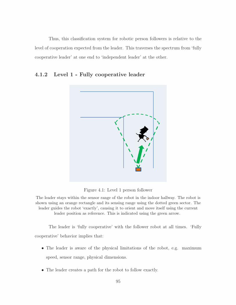
Thus, this classification system for robotic person followers is relative to the

level of cooperation expected from the leader. This traverses the spectrum from ‘fully

cooperative leader’ at one end to ‘independent leader’ at the other.

4.1.2 Level 1 - Fully cooperative leader

Figure 4.1: Level 1 person follower

The leader stays within the sensor range of the robot in the indoor hallway. The robot isshown using an orange rectangle and its sensing range using the dotted green sector. Theleader guides the robot ‘exactly’, causing it to orient and move itself using the current

leader position as reference. This is indicated using the green arrow.

The leader is ‘fully cooperative’ with the follower robot at all times. ‘Fully

cooperative’ behavior implies that:

• The leader is aware of the physical limitations of the robot, e.g. maximum

speed, sensor range, physical dimensions.

• The leader creates a path for the robot to follow exactly.

95

• The leader stays within sensor range of the robot.

• The leader stays detectable to the robot.

• The leader ensures that he/she is never occluded from view of the robot sensor,

i.e. there are no obstacles between the leader and the robot.

This scenario is illustrated in Figure 4.1. The robot, at any given time during a trial

run, turns to orient itself with the leader and translates to a desired distance relative

to the leader. The leader is expected to fully guide the robot at all times and ensure

that his/her path is capable of being emulated by the robotic follower. Moreover, the

‘no occlusion’ conditions require the leader to maintain a direct line of sight to the

robot at all times.

Though this scenario is not practical for a person following service robot, it

has been effectively used to test algorithms such as stereo-based depth estimation

and segmentation, and human-robot interaction paradigms. An interesting feature

tracking and stereo based Level-1 person follower was demonstrated by Chen [17].

Brookshire [34] used a combination of HOG features [37] and particle filtering to follow

a person outdoors over a large distance and through challenges such as inclement

weather. Kirby [2] introduced an interactive following paradigm where the robot

used voice to communicate with the leader when the leader went out of sensor range.

4.1.3 Level 2 - Partially cooperative leader

The leader cooperates with the follower, but may occasionally be occluded by

the environment. The straight line to the leader may also be hindered by low height

stationary obstacles. Hence the term ‘partially cooperative’ leader. During Level-2

following:

96

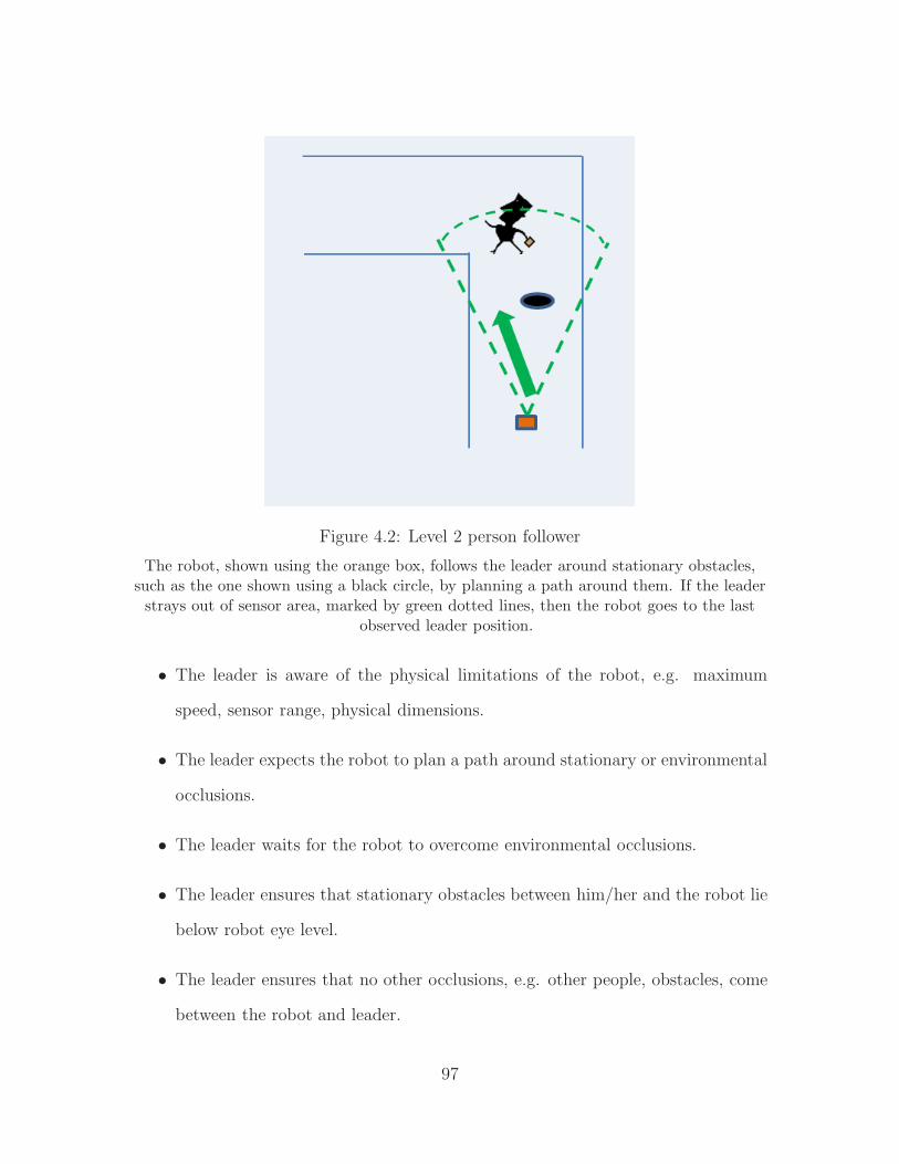
Figure 4.2: Level 2 person follower

The robot, shown using the orange box, follows the leader around stationary obstacles,such as the one shown using a black circle, by planning a path around them. If the leaderstrays out of sensor area, marked by green dotted lines, then the robot goes to the last

observed leader position.

• The leader is aware of the physical limitations of the robot, e.g. maximum

speed, sensor range, physical dimensions.

• The leader expects the robot to plan a path around stationary or environmental

occlusions.

• The leader waits for the robot to overcome environmental occlusions.

• The leader ensures that stationary obstacles between him/her and the robot lie

below robot eye level.

• The leader ensures that no other occlusions, e.g. other people, obstacles, come

between the robot and leader.

97

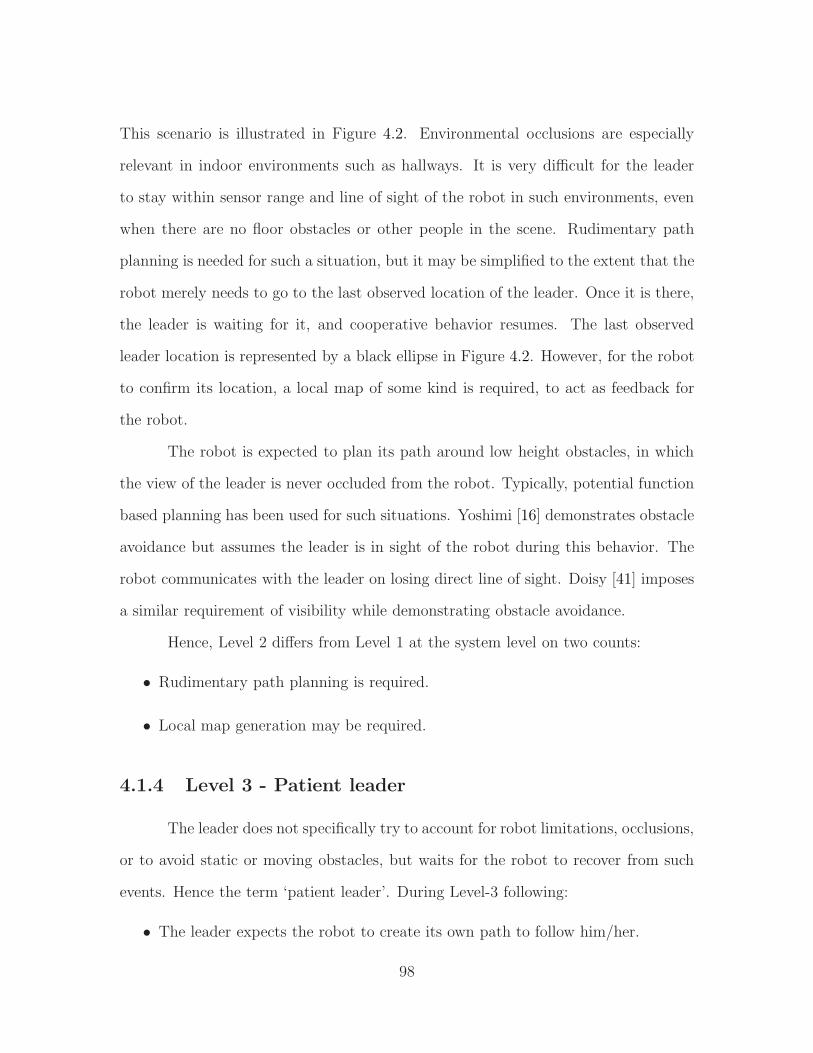
This scenario is illustrated in Figure 4.2. Environmental occlusions are especially

relevant in indoor environments such as hallways. It is very difficult for the leader

to stay within sensor range and line of sight of the robot in such environments, even

when there are no floor obstacles or other people in the scene. Rudimentary path

planning is needed for such a situation, but it may be simplified to the extent that the

robot merely needs to go to the last observed location of the leader. Once it is there,

the leader is waiting for it, and cooperative behavior resumes. The last observed

leader location is represented by a black ellipse in Figure 4.2. However, for the robot

to confirm its location, a local map of some kind is required, to act as feedback for

the robot.

The robot is expected to plan its path around low height obstacles, in which

the view of the leader is never occluded from the robot. Typically, potential function

based planning has been used for such situations. Yoshimi [16] demonstrates obstacle

avoidance but assumes the leader is in sight of the robot during this behavior. The

robot communicates with the leader on losing direct line of sight. Doisy [41] imposes

a similar requirement of visibility while demonstrating obstacle avoidance.

Hence, Level 2 differs from Level 1 at the system level on two counts:

• Rudimentary path planning is required.

• Local map generation may be required.

4.1.4 Level 3 - Patient leader

The leader does not specifically try to account for robot limitations, occlusions,

or to avoid static or moving obstacles, but waits for the robot to recover from such

events. Hence the term ‘patient leader’. During Level-3 following:

• The leader expects the robot to create its own path to follow him/her.

98

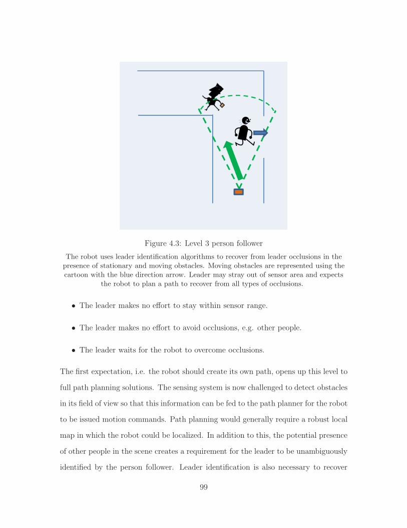
Figure 4.3: Level 3 person follower

The robot uses leader identification algorithms to recover from leader occlusions in thepresence of stationary and moving obstacles. Moving obstacles are represented using thecartoon with the blue direction arrow. Leader may stray out of sensor area and expects

the robot to plan a path to recover from all types of occlusions.

• The leader makes no effort to stay within sensor range.

• The leader makes no effort to avoid occlusions, e.g. other people.

• The leader waits for the robot to overcome occlusions.

The first expectation, i.e. the robot should create its own path, opens up this level to

full path planning solutions. The sensing system is now challenged to detect obstacles

in its field of view so that this information can be fed to the path planner for the robot

to be issued motion commands. Path planning would generally require a robust local

map in which the robot could be localized. In addition to this, the potential presence

of other people in the scene creates a requirement for the leader to be unambiguously

identified by the person follower. Leader identification is also necessary to recover

99

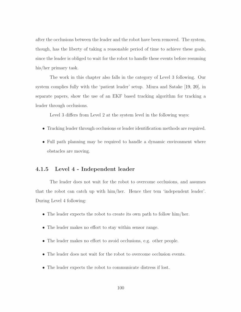
after the occlusions between the leader and the robot have been removed. The system,

though, has the liberty of taking a reasonable period of time to achieve these goals,

since the leader is obliged to wait for the robot to handle these events before resuming

his/her primary task.

The work in this chapter also falls in the category of Level 3 following. Our

system complies fully with the ‘patient leader’ setup. Miura and Satake [19, 20], in

separate papers, show the use of an EKF based tracking algorithm for tracking a

leader through occlusions.

Level 3 differs from Level 2 at the system level in the following ways:

• Tracking leader through occlusions or leader identification methods are required.

• Full path planning may be required to handle a dynamic environment where

obstacles are moving.

4.1.5 Level 4 - Independent leader

The leader does not wait for the robot to overcome occlusions, and assumes

that the robot can catch up with him/her. Hence ther tem ‘independent leader’.

During Level 4 following:

• The leader expects the robot to create its own path to follow him/her.

• The leader makes no effort to stay within sensor range.

• The leader makes no effort to avoid occlusions, e.g. other people.

• The leader does not wait for the robot to overcome occlusion events.

• The leader expects the robot to communicate distress if lost.

100

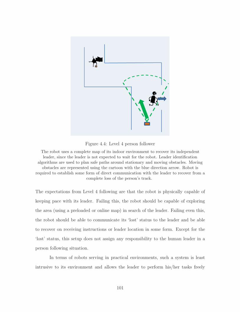
Figure 4.4: Level 4 person follower

The robot uses a complete map of its indoor environment to recover its independentleader, since the leader is not expected to wait for the robot. Leader identification

algorithms are used to plan safe paths around stationary and moving obstacles. Movingobstacles are represented using the cartoon with the blue direction arrow. Robot is

required to establish some form of direct communication with the leader to recover from acomplete loss of the person’s track.

The expectations from Level 4 following are that the robot is physically capable of

keeping pace with its leader. Failing this, the robot should be capable of exploring

the area (using a preloaded or online map) in search of the leader. Failing even this,

the robot should be able to communicate its ‘lost’ status to the leader and be able

to recover on receiving instructions or leader location in some form. Except for the

‘lost’ status, this setup does not assign any responsibility to the human leader in a

person following situation.

In terms of robots serving in practical environments, such a system is least

intrusive to its environment and allows the leader to perform his/her tasks freely

101

without having to continuously check whether the robot has kept pace. A Level 4

system has currently not been completely realized. Gross [11] and Weinrich [36, 35] et

al. demonstrate an interesting system for socially assistive robots to help the elderly

but do not discuss its ability to plan paths in a dynamic environment with moving

obstacles. Kirby [2] proposes interaction with the human when the robot is lost, but

the condition for being ‘lost’ is limited to the leader moving out of sensor range. This

is severely limiting for indoor navigation, as discussed earlier.

Level 4 differs from Level 3 at the system level in the following ways:

• A complete mapping solution is required.

• Sophisticated human-robot interaction is required to recover from distress situ-

ations.

In summary, the proposed classification system describes person following in

terms of the expectations from the leader. Such a classification system allows roboti-

cists working within each level to focus on useful subsystems such as mapping and

estimation, while freeing them from the expectation of presenting a complete system.

At the same time, it allows the human working with the robot to know exactly when

active ‘leadership’ is required for the interaction to be fruitful. Presumably, commer-

cial versions of service robots could supply information about the robot capabilities

in terms of the leader using a system similar to the one proposed here.

With this in mind, the remaining sections of this chapter focus on the devel-

opment and implementation of techniques for the proposed Level 3 follower.

102

4.2 Leader tracking using color descriptors

An important module for a Level-3 person following robot is its ability to track

the leader through occlusions. The solution proposed here combines the strengths

of the Microsoft Kinect skeletal tracker with a color descriptor generated using a

combination of two colorspaces: HSI and L*a*b* (CIE 1976). The former provides a

temporal tracking output based on depth data from the Kinect RGB-D sensor. The

latter is used when the temporal track of a skeleton has been lost, i.e. the person

has been occluded. The Kinect skeletal tracker’s features are explained in the Section

4.2.1, followed by an explanation of the appearance based descriptor which makes it

possible to track the leader through short and long term occlusions. Results for this

subsystem are provided at the end of this section.

4.2.1 Kinect skeletal tracking

Following the commercial release of the Microsoft Kinect [89], Microsoft re-

leased a SDK [90] to allow programmers and researchers to interface with this RGB-D

sensor. Function calls from the Kinect SDK have since been integrated into the com-

puter vision library Blepo, which has been used for this software implementation of

the person follower. The Kinect SDK contains an implementation of the skeletal

tracker. This algorithm, first proposed in [31], uses depth information to predict the

position of 3D body parts. The skeletal tracker has the ability to keep track of up to

six people (skeletons) in the field of view of the Kinect camera.

A skeleton is defined by the algorithm as a configuration consisting of 20 joints

and 19 bones. The joints and bones which comprise the Kinect skeleton are shown in

Figure 4.5. Information about the skeletons is stored in a data structure. Relevant

information stored per skeleton is as follows:

103

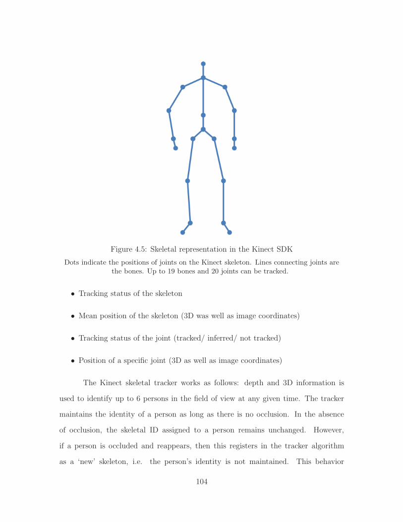
Figure 4.5: Skeletal representation in the Kinect SDK

Dots indicate the positions of joints on the Kinect skeleton. Lines connecting joints arethe bones. Up to 19 bones and 20 joints can be tracked.

• Tracking status of the skeleton

• Mean position of the skeleton (3D was well as image coordinates)

• Tracking status of the joint (tracked/ inferred/ not tracked)

• Position of a specific joint (3D as well as image coordinates)

The Kinect skeletal tracker works as follows: depth and 3D information is

used to identify up to 6 persons in the field of view at any given time. The tracker

maintains the identity of a person as long as there is no occlusion. In the absence

of occlusion, the skeletal ID assigned to a person remains unchanged. However,

if a person is occluded and reappears, then this registers in the tracker algorithm

as a ‘new’ skeleton, i.e. the person’s identity is not maintained. This behavior

104

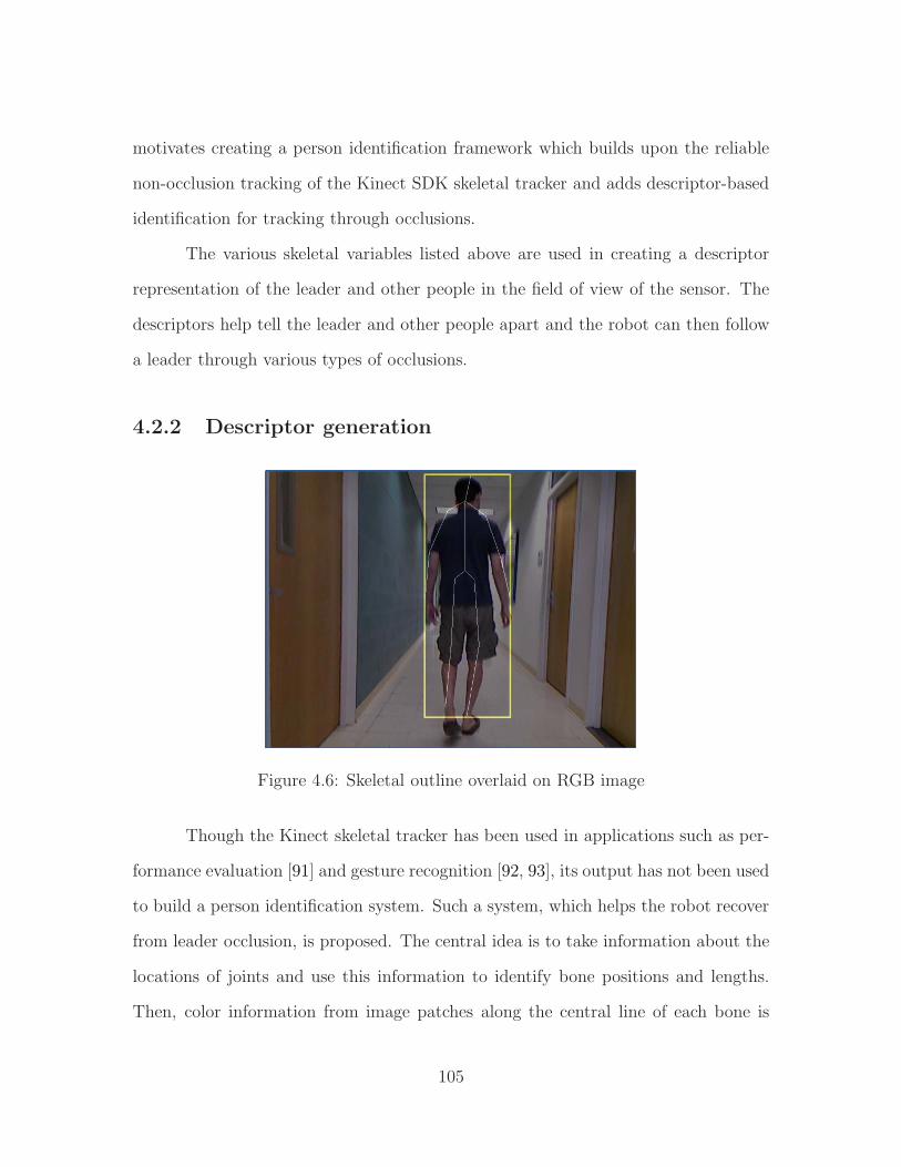
motivates creating a person identification framework which builds upon the reliable

non-occlusion tracking of the Kinect SDK skeletal tracker and adds descriptor-based

identification for tracking through occlusions.

The various skeletal variables listed above are used in creating a descriptor

representation of the leader and other people in the field of view of the sensor. The

descriptors help tell the leader and other people apart and the robot can then follow

a leader through various types of occlusions.

4.2.2 Descriptor generation

Figure 4.6: Skeletal outline overlaid on RGB image

Though the Kinect skeletal tracker has been used in applications such as per-

formance evaluation [91] and gesture recognition [92, 93], its output has not been used

to build a person identification system. Such a system, which helps the robot recover

from leader occlusion, is proposed. The central idea is to take information about the

locations of joints and use this information to identify bone positions and lengths.

Then, color information from image patches along the central line of each bone is

105

collected into a descriptor. The Kinect tracker identifies the location of 20 joints,

hence 19 bones can be identified. Four color values are calculated per bone, to yield a

descriptor of 19×4 = 76 elements. Descriptors are matched using Euclidean distance

and an empirically observed threshold is used to classify the observed descriptor as

leader or otherwise.

The color information extracted per bone are the chromaticity components of

the HSI and CIE L*a*b* color space. Both color spaces separate the color component

from luminosity or brightness, which makes them more robust to lighting changes such

as variance in indoor illumination and shadows.

HSI (Hue-Saturation-Intensity) is a cylindrical color space, whose conversion

from RGB is specified in [94] as:

H = cos−1 0.5·(R−G)+(R−B)√(R−G)2+(R−B)(G−B)

S = 1−(

3R+G+B

)

·min(R,G,B)

I = R+G+B3

In HSI, ‘I’ is the intensity component which is discarded when the person-specific

descriptor is being formulated.

The CIE L*a*b* (also known as CIE 1976) color space derives from the CIE

XYZ (CIE 1931) color space and was designed to mimic the response of the human

eye to color. L* is the luminosity component, which is discarded when the descriptor

is formed. Conversion from RGB to L*a*b* is a two step process, comprising of con-

version from RGB to XYZ and from XYZ to LAB. Formulae for the two conversions

106

are given here [95]. RGB is first converted to XYZ using [96]:

X = 0.4124 · R + 0.3576 ·G+ 0.1805 ·B

Y = 0.2126 · R + 0.7152 ·G+ 0.0722 ·B

Z = 0.0193 · R + 0.1192 ·G+ 0.9505 ·B

XYZ values are then converted to L*a*b* values using

L∗ =

116 · (Y/Yn)1

3 − 16 for(Y/Yn) > 0.008856

903.3 · (Y/Yn) otherwise

a∗ = 500 · (f(X/Xn)− f(Y/Yn))

b∗ = 200 · (f(Y/Yn)− f(Z/Zn))

where

f(t) =

t1

3 for t > 0.08856

7.787 · t + 16/116 otherwise

and where Xn = Yn = Zn = 13is the tristimulus point (white) of the XYZ color space.

To extract HSI and L*a*b* components to form a skeletal descriptor, the

end points of a bone in the RGB image are considered. If the corresponding depth

values for these points lie within an acceptable range of the average depth of the

person (returned by the skeletal tracker), then the color extraction step is carried

out; otherwise, color values for that bone are all set to −1. The latter is used to

indicate that the tracked bone position may lie outside the actual outline of the

person. In Figure 4.6, an example of well and poorly detected bone positions is seen.

The observed misalignment clearly motivates this filtering step.

For bones which have been tracked well, image patches which align with the

orientations of these bones are extracted. An example of this is shown in Figure 4.7.

107

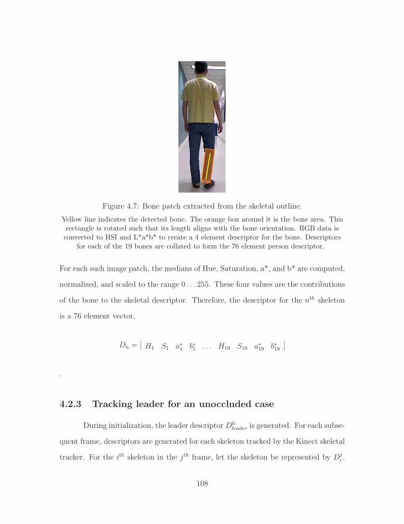
Figure 4.7: Bone patch extracted from the skeletal outline.

Yellow line indicates the detected bone. The orange box around it is the bone area. Thisrectangle is rotated such that its length aligns with the bone orientation. RGB data isconverted to HSI and L*a*b* to create a 4 element descriptor for the bone. Descriptors

for each of the 19 bones are collated to form the 76 element person descriptor.

For each such image patch, the medians of Hue, Saturation, a*, and b* are computed,

normalized, and scaled to the range 0 . . . 255. These four values are the contributions

of the bone to the skeletal descriptor. Therefore, the descriptor for the nth skeleton

is a 76 element vector,

Dn = [ H1 S1 a∗1 b∗1 . . . H19 S19 a∗19 b∗19 ]

.

4.2.3 Tracking leader for an unoccluded case

During initialization, the leader descriptor D0leader is generated. For each subse-

quent frame, descriptors are generated for each skeleton tracked by the Kinect skeletal

tracker. For the ith skeleton in the jth frame, let the skeleton be represented by Dji .

108

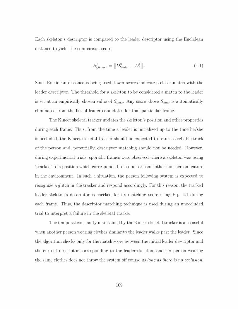
Each skeleton’s descriptor is compared to the leader descriptor using the Euclidean

distance to yield the comparison score,

Sji,leader =

∥

∥D0leader −Dj

i

∥

∥ . (4.1)

Since Euclidean distance is being used, lower scores indicate a closer match with the

leader descriptor. The threshold for a skeleton to be considered a match to the leader

is set at an empirically chosen value of Smax. Any score above Smax is automatically

eliminated from the list of leader candidates for that particular frame.

The Kinect skeletal tracker updates the skeleton’s position and other properties

during each frame. Thus, from the time a leader is initialized up to the time he/she

is occluded, the Kinect skeletal tracker should be expected to return a reliable track

of the person and, potentially, descriptor matching should not be needed. However,

during experimental trials, sporadic frames were observed where a skeleton was being

‘tracked’ to a position which corresponded to a door or some other non-person feature

in the environment. In such a situation, the person following system is expected to

recognize a glitch in the tracker and respond accordingly. For this reason, the tracked

leader skeleton’s descriptor is checked for its matching score using Eq. 4.1 during

each frame. Thus, the descriptor matching technique is used during an unoccluded

trial to interpret a failure in the skeletal tracker.

The temporal continuity maintained by the Kinect skeletal tracker is also useful

when another person wearing clothes similar to the leader walks past the leader. Since

the algorithm checks only for the match score between the initial leader descriptor and

the current descriptor corresponding to the leader skeleton, another person wearing

the same clothes does not throw the system off course as long as there is no occlusion.

109

4.2.4 Detecting occlusions and leader reappearance

Figure 4.8: Example of self-occlusion

When the person turns, skeletal information is overlaid poorly, and descriptor is adverselyaffected by this misalignment. Thus, turning or ‘self-occlusion’ needs to be avoided by the

descriptor matching algorithm.

The descriptor matching algorithm is most useful in leader reidentification

after the occlusion has been removed, i.e. when the leader reappears. As explained

in Section 4.2.1, the Kinect skeletal tracker cannot reestablish leader identity when a

leader has reappeared after an occluding event. Occluding events can be categorized

as follows:

• Self-occlusion: Leader turns while fully in view of the Kinect

• Sensor occlusion: Leader moves out of of the field of view of the Kinect

• Obstacle or person occlusion: Other people or objects in the field of view occlude

the leader

Of these items, the first, i.e. self-occlusion, is a special event based on the

descriptor generation method. The Kinect skeletal tracker maintains track of the

110

leader when the leader is turning. However, as explained in the previous section,

sporadic tracking errors by the Kinect SDK are being avoided by comparing the

current leader descriptor Djleader to the initialized leader descriptor D0

leader. As seen

in Figure 4.8, however, the pose of the skeleton is often poorly estimated when the

leader is turning. Hence, the extracted bone patches are poorly aligned with the

actual positions of bones. This can lead to a very poor match score between Djleader

and D0leader. It is necessary to prevent this score from leading to the inference that

the leader is either lost or occluded by another person.

Figure 4.9: Using bone angles to infer self-occlusion.

As a person turns, the four bone angles indicated using red arrows in the left image, showsharp deviations from their normal values, as highlighted by the purple box in the rightimage. Thus, initializing bone angles and comparing them against a deviation threshold

allows the system to infer self-occlusion.

To remedy this, self-occlusion is inferred and the descriptor matching is ‘turned

off’ until self-occlusion has terminated, i.e. leader no longer has a profile view as seen

from the Kinect. It was found that four angles between bones, indicated in Figure

4.9 were good indicators for detecting when the leader was turning. The graph to

the right in the figure shows the variation in these angles for a trial where the leader

111

turned once. The purple box shows the frames where the leader turned 180◦. These

frames clearly coincide with the widest variation in bone angle values. This type

of trend was consistently observed during trials, and the indicated bone angles are

computed and checked for being within bounds during each frame to help the system

overcome leader self-occlusion.

The other two types of occlusion, sensor and person occlusion, are dealt with

using a common descriptor-based mechanism. They are inferred when the skeletal

tracker registers the initialized leader skeleton ID as being ‘not tracked’. When this

event occurs, the algorithm begins to compare all tracked person descriptors with the

original leader descriptor D0leader. This process continues over multiple frames until

the one of the descriptors satisfies the threshold Smax. At this point, the occlusion

is inferred to have been removed. The skeletal ID of the closely matching descriptor

is assigned as the new leader ID, and the reference leader descriptor is updated to

D0leader = Dn

leader, where the current frame number is n.

It may be argued that temporal tracks of the leader could also be used to

achieve recovery through occlusions. This approach is tenable and has been used in

[19, 20]. But the problem with such approaches, despite their reliance on sophisticated

motion models, is that they are not guaranteed to succeed over long term occlusions.

This is especially true for tracking a person, since there may be arbitrary direction

and position changes during the period of the occlusion. Using an appearance based

method such as descriptors frees the algorithm from having to generate a reliable and

robust filtering output.

Having motivated and explained the descriptor algorithm, its performance is

evaluated in the next section.

112

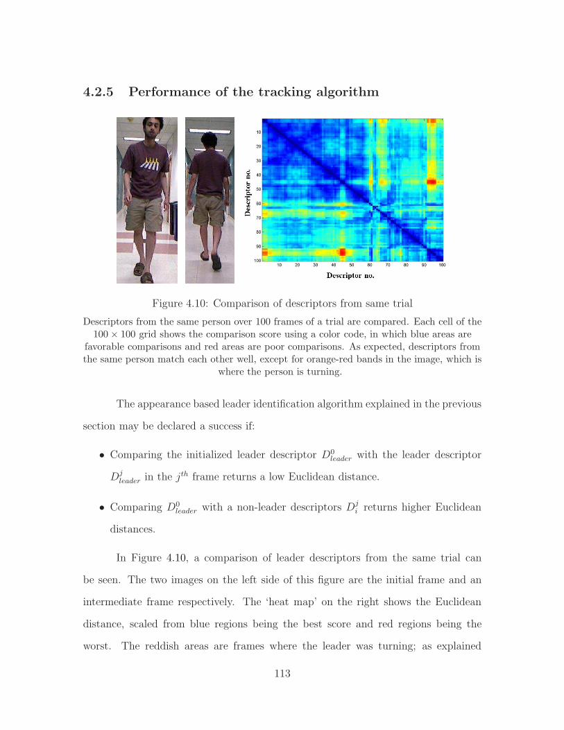
4.2.5 Performance of the tracking algorithm

Figure 4.10: Comparison of descriptors from same trial

Descriptors from the same person over 100 frames of a trial are compared. Each cell of the100× 100 grid shows the comparison score using a color code, in which blue areas are

favorable comparisons and red areas are poor comparisons. As expected, descriptors fromthe same person match each other well, except for orange-red bands in the image, which is

where the person is turning.

The appearance based leader identification algorithm explained in the previous

section may be declared a success if:

• Comparing the initialized leader descriptor D0leader with the leader descriptor

Djleader in the jth frame returns a low Euclidean distance.

• Comparing D0leader with a non-leader descriptors Dj

i returns higher Euclidean

distances.

In Figure 4.10, a comparison of leader descriptors from the same trial can

be seen. The two images on the left side of this figure are the initial frame and an

intermediate frame respectively. The ‘heat map’ on the right shows the Euclidean

distance, scaled from blue regions being the best score and red regions being the

worst. The reddish areas are frames where the leader was turning; as explained

113

in the previous section, no occlusion inference is made during these frames. The

horizontal and vertical axes are both frame numbers from the trial.

Figure 4.11: Comparison of descriptors from different trials

Descriptors from two different trials, using 100 frames each, are compared. Each cell ofthe 100 × 100 grid shows the comparison score, in which blue areas are favorable

comparisons and red areas are poor comparisons. As expected, descriptors two trialsmatch each other poorly, since the person is wearing different clothes in each.

The heat map helps visualize the performance of the descriptor generation and

matching method when dissimilar descriptors are being compared. See Figure 4.11, in

which the heat map is scaled to the same limits as Figure 4.10. In this dataset, leader

descriptors generated during one trial were compared to leader descriptors from a

different trial. As can be seen in the images on the left of the figure, the clothing

worn by the leader in these trials is different. The heat map on the right shows that

the descriptors are dissimilar, evidenced by the red regions on the map.

114

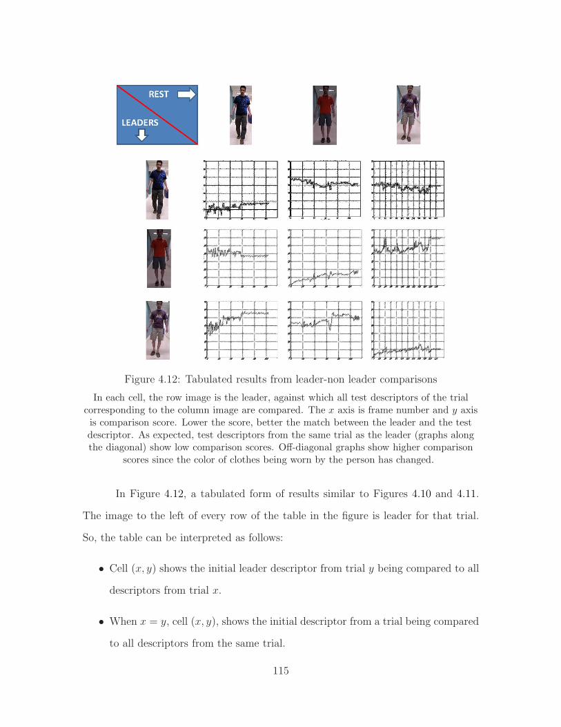
Figure 4.12: Tabulated results from leader-non leader comparisons

In each cell, the row image is the leader, against which all test descriptors of the trialcorresponding to the column image are compared. The x axis is frame number and y axisis comparison score. Lower the score, better the match between the leader and the testdescriptor. As expected, test descriptors from the same trial as the leader (graphs alongthe diagonal) show low comparison scores. Off-diagonal graphs show higher comparison

scores since the color of clothes being worn by the person has changed.

In Figure 4.12, a tabulated form of results similar to Figures 4.10 and 4.11.

The image to the left of every row of the table in the figure is leader for that trial.

So, the table can be interpreted as follows:

• Cell (x, y) shows the initial leader descriptor from trial y being compared to all

descriptors from trial x.

• When x = y, cell (x, y), shows the initial descriptor from a trial being compared

to all descriptors from the same trial.

115

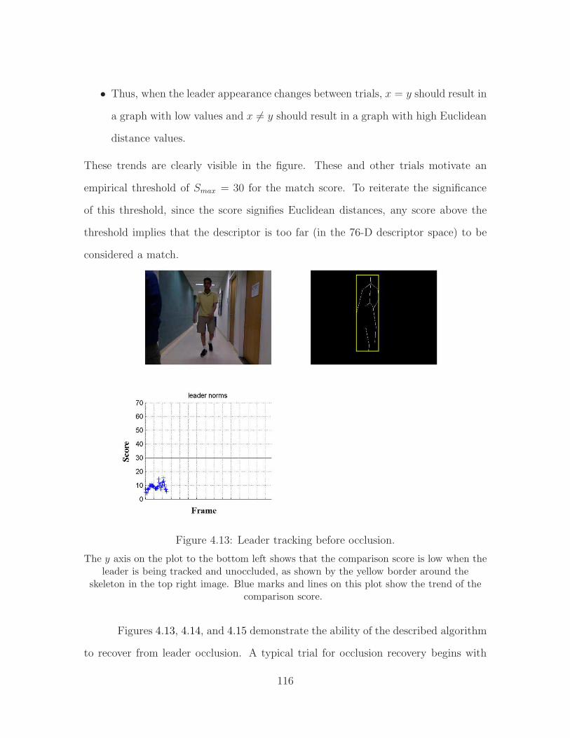
• Thus, when the leader appearance changes between trials, x = y should result in

a graph with low values and x 6= y should result in a graph with high Euclidean

distance values.

These trends are clearly visible in the figure. These and other trials motivate an

empirical threshold of Smax = 30 for the match score. To reiterate the significance

of this threshold, since the score signifies Euclidean distances, any score above the

threshold implies that the descriptor is too far (in the 76-D descriptor space) to be

considered a match.

Figure 4.13: Leader tracking before occlusion.

The y axis on the plot to the bottom left shows that the comparison score is low when theleader is being tracked and unoccluded, as shown by the yellow border around the

skeleton in the top right image. Blue marks and lines on this plot show the trend of thecomparison score.

Figures 4.13, 4.14, and 4.15 demonstrate the ability of the described algorithm

to recover from leader occlusion. A typical trial for occlusion recovery begins with

116

Figure 4.14: Detected occlusion.

The y axis on the plot to the bottom right shows that a non-leader skeleton has beendetected, as evidenced by the high comparison scores shown by red marks and connectinglines. An occlusion has been detected, as shown by the lack of the yellow ‘leader’ borderaround the skeleton in the top right image. Blue marks and lines on the leader plot to the

bottom left remain unchanged from Figure 4.13 since the leader is not visible.

the leader being initialized and leader descriptor being generated. The plot at the

bottom left of each of the figures shows the comparison score of the current leader

descriptor with the initialized leader descriptor. As seen in Figure 4.13, these values

are typically well below the threshold of Smax = 30.

When another person occludes the leader, as seen in Figure 4.13, the Kinect

skeletal tracker tags the leader skeleton ID as being ‘not tracked’. The algorithm now

switches to its leader recovery phase, in which all detected skeletons are compared with

the initialized leader descriptor. If the match between a detected skeleton descriptor

and the leader descriptor is above the threshold, then the skeleton is rejected as a

117

Figure 4.15: Leader recovery after occusion.

The leader is recovered from the occlusion in Figure 4.14, as shown by the reappearance ofa blue mark and connecting line on the leader plot on the bottom left. The y axis on theplot to the bottom right shows that the non-leader skeleton consistently returned high

comparison scores, as evidenced by red marks and connecting lines.

possible reappearance of the leader after occlusion. Figure 4.14 shows this occlusion

detection mechanism at work. The plot at the bottom right of this figure shows

comparison scores for inferred non-leader skeletons. It can be seen that the values

are consistently above the threshold for a number of frames in which the occluding

skeleton is being detected by the skeletal tracker.

Figure 4.15 demonstrates occlusion recovery at work. After a number of

frames, the leader reappears in the field of view. During this frame, both the leader

and the occluding skeleton are detected. The algorithm compares both skeletal de-

scriptors to the initialized leader descriptor and finds that the reappeared leader’s

118

descriptor matches the initial descriptor to well below the threshold. The skeleton

which satisfies this condition is then tagged as the reappeared leader for the person

follower.

In all figures, the yellow box is indicative of the skeleton which is being detected

as the leader. Thus, this data demonstrates the effectiveness of the appearance based

descriptor in occlusion detection and recovery.

With this module in place, the next task for the person follower is to map

its environment locally, so that robot control and path planning can be implemented

when required.

119

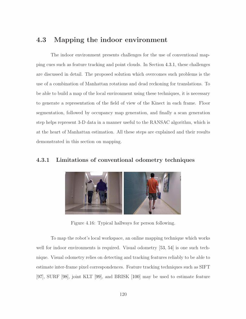
4.3 Mapping the indoor environment

The indoor environment presents challenges for the use of conventional map-

ping cues such as feature tracking and point clouds. In Section 4.3.1, these challenges

are discussed in detail. The proposed solution which overcomes such problems is the

use of a combination of Manhattan rotations and dead reckoning for translations. To

be able to build a map of the local environment using these techniques, it is necessary

to generate a representation of the field of view of the Kinect in each frame. Floor

segmentation, followed by occupancy map generation, and finally a scan generation

step helps represent 3-D data in a manner useful to the RANSAC algorithm, which is

at the heart of Manhattan estimation. All these steps are explained and their results

demonstrated in this section on mapping.

4.3.1 Limitations of conventional odometry techniques

Figure 4.16: Typical hallways for person following.

To map the robot’s local workspace, an online mapping technique which works

well for indoor environments is required. Visual odometry [53, 54] is one such tech-

nique. Visual odometry relies on detecting and tracking features reliably to be able to

estimate inter-frame pixel correspondences. Feature tracking techniques such as SIFT

[97], SURF [98], joint KLT [99], and BRISK [100] may be used to estimate feature

120

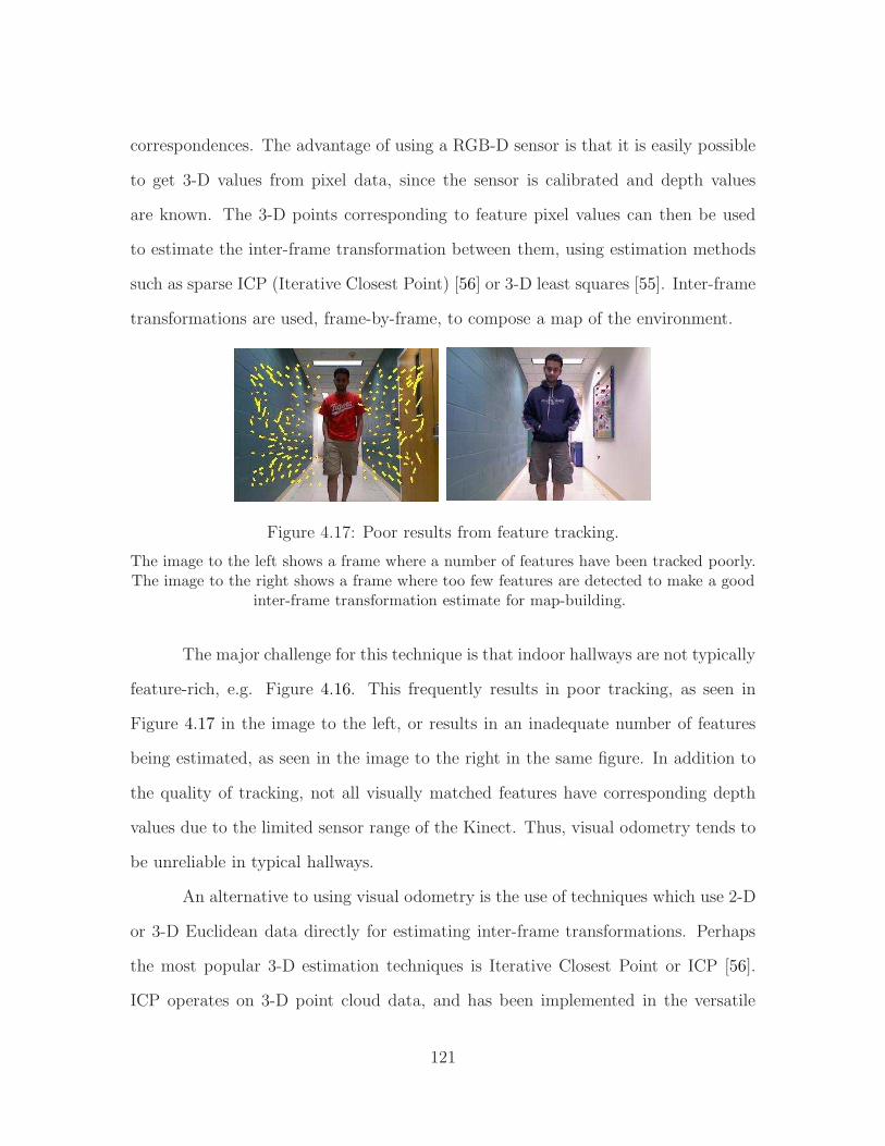
correspondences. The advantage of using a RGB-D sensor is that it is easily possible

to get 3-D values from pixel data, since the sensor is calibrated and depth values

are known. The 3-D points corresponding to feature pixel values can then be used

to estimate the inter-frame transformation between them, using estimation methods

such as sparse ICP (Iterative Closest Point) [56] or 3-D least squares [55]. Inter-frame

transformations are used, frame-by-frame, to compose a map of the environment.

Figure 4.17: Poor results from feature tracking.

The image to the left shows a frame where a number of features have been tracked poorly.The image to the right shows a frame where too few features are detected to make a good

inter-frame transformation estimate for map-building.

The major challenge for this technique is that indoor hallways are not typically

feature-rich, e.g. Figure 4.16. This frequently results in poor tracking, as seen in

Figure 4.17 in the image to the left, or results in an inadequate number of features

being estimated, as seen in the image to the right in the same figure. In addition to

the quality of tracking, not all visually matched features have corresponding depth

values due to the limited sensor range of the Kinect. Thus, visual odometry tends to

be unreliable in typical hallways.

An alternative to using visual odometry is the use of techniques which use 2-D

or 3-D Euclidean data directly for estimating inter-frame transformations. Perhaps

the most popular 3-D estimation techniques is Iterative Closest Point or ICP [56].

ICP operates on 3-D point cloud data, and has been implemented in the versatile

121

Point Cloud Library (PCL) [101] and the stand-alone library LibICP[102]. Spatial

configuration of point clouds can be exploited to find 3-D features in the data, an

approach outlined in Fast Point Feature Histograms (FPFH) [103]. Scan matching

[57, 58] is a 2-D technique in which the plan view of the floor is generated (usually

using range scanners) and two such views are matched using iterative techniques

which minimize an error function. The output of all of these depth-based methods is

an estimate of rotation and translation between frames.

However, the problem with using depth-based methods is very similar to that

in using visual odometry: namely, the absence of depth ‘features’ which can be be

useful in estimating the inter-frame transformation. The limitation is especially severe

when it comes to inferring translations, since the robot is moving between two parallel

walls and successive scans or 3-D point clouds are very similar to each other in such

environments. This makes it very difficult for any algorithm to tell apart genuine,

usable variations in the hallway data (such as lintels) from sensor noise, and this

exacerbates the quality of the transformation estimate.

See Figure 4.18 for an example of a poor depth-based estimate. The two

stacked images to the left in this figure show the raw data being processed by the

Diosi’s scan matching algorithm [57]. The map to the right shows that the data from

these frames has been stitched together with considerable drift.

Although a combination of visual odometry and scan matching provided oc-

casional sequences of frames where the map was of acceptable quality, a recurring

observation was that of frames such as the one in Figure 4.18, which would throw

the map completely off course. The precautionary measure in map building was to

reset the map when large rotations or translations were detected; however, this in-

consistency was undesirable since the map was to be ultimately used by the path

planner.

122

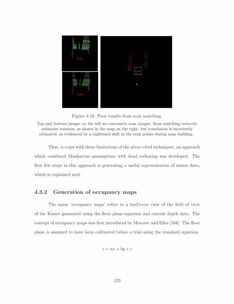
Figure 4.18: Poor results from scan matching.

Top and bottom images on the left are successive scan images. Scan matching correctlyestimates rotation, as shown in the map on the right, but translation is incorrectly

estimated, as evidenced by a rightward shift in the scan points during map building.

Thus, to cope with these limitations of the above cited techniques, an approach

which combined Manhattan assumptions with dead reckoning was developed. The

first few steps in this approach is generating a useful representation of sensor data,

which is explained next.

4.3.2 Generation of occupancy maps

The name ‘occupancy maps’ refers to a bird’s-eye view of the field of view

of the Kinect generated using the floor plane equation and current depth data. The

concept of occupancy maps was first introduced by Moravec and Elfes [104]. The floor

plane is assumed to have been calibrated before a trial using the standard equation

z = ax+ by + c

123

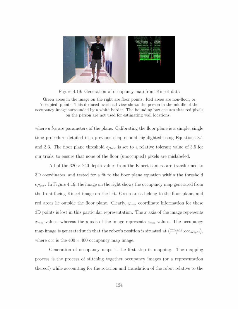
Figure 4.19: Generation of occupancy map from Kinect data

Green areas in the image on the right are floor points. Red areas are non-floor, or‘occupied’ points. This deduced overhead view shows the person in the middle of the

occupancy image surrounded by a white border. The bounding box ensures that red pixelson the person are not used for estimating wall locations.

where a,b,c are parameters of the plane. Calibrating the floor plane is a simple, single

time procedure detailed in a previous chapter and highlighted using Equations 3.1

and 3.3. The floor plane threshold ǫfloor is set to a relative tolerant value of 3.5 for

our trials, to ensure that none of the floor (unoccupied) pixels are mislabeled.

All of the 320× 240 depth values from the Kinect camera are transformed to

3D coordinates, and tested for a fit to the floor plane equation within the threshold

ǫfloor. In Figure 4.19, the image on the right shows the occupancy map generated from

the front-facing Kinect image on the left. Green areas belong to the floor plane, and

red areas lie outside the floor plane. Clearly, ymm coordinate information for these

3D points is lost in this particular representation. The x axis of the image represents

xmm values, whereas the y axis of the image represents zmm values. The occupancy

map image is generated such that the robot’s position is situated at(

occwidth

2.occheight

)

,

where occ is the 400× 400 occupancy map image.

Generation of occupancy maps is the first step in mapping. The mapping

process is the process of stitching together occupancy images (or a representation

thereof) while accounting for the rotation and translation of the robot relative to the

124

reference occupancy image for the map.

4.3.3 Scan generation

Figure 4.20: Generation of polar scans from occupancy maps

A set of (r, θ) pairs is generated with respect to the robot position indicated by the yellowsquare at the bottom of the image. Angle values are evenly spaced in the range 0 . . . 180.Dotted orange lines indicate the shortest radial distance to a non-floor point for some ofthe angle values. The person bounding box, shown using a white rectangle, is excluded

from this process.

Estimating Manhattan rotation requires estimating wall lines in an image and

computing the rotation of these lines relative to the wall line orientation at the refer-

ence map frame. The occupancy image could be used directly for wall line estimation.

However, a typical occupancy map, e.g. Figure 4.19, contains a large number of closely

clustered points. Line fitting algorithms working with such data may not converge to

125

the best line estimates. With a large number of points in the raw occupancy data, it

may take longer for line fitting to converge. Scan generation is an intermediate step

which is used to reduce the number of points to be passed on to the line fitting, which

is the next step in mapping.

Laser range finders generated scans which were often used for mapping [57]

and pose estimation [105]. Inspired by the form of the raw data from laser range

scanners, occupancy map data is reduced to a smaller number of points using the

(r, θ) representation. The process is sketched in Figure 4.20. The robot, shown in

yellow, is at the bottom-center of the occupancy map. the 180◦ range relative to this

point is scanned with a user-defined resolution (in this case, resscan = 0.2◦, and the

closest occupied (red) pixel along each direction (shown using dotted orange lines) is

added to the list of scan points. To avoid the leader and other detected persons being

added to such a list, red pixels belonging to skeletal tracks (surrounded by a white

box in the image) are ignored during scan generation.

At the end of scan generation, a list of points (ri, θi), i = 1 . . . 180/resscan, is

available for line fitting and subsequently for estimating robot pose relative to the

reference pose.

4.3.4 RANSAC for multiple lines

Given a set of scan points, line equations which fit the data are desired. The

requirement for the line estimation algorithm is that it should be able to find all wall

lines in the raw data, which is the set of scan points. This set of wall lines is used in

estimating the pose of the robot relative to its pose at the time of map initialization

or reset. Each line in the set of lines is estimated using a robust model parameter

estimation technique called RANSAC [106].

126

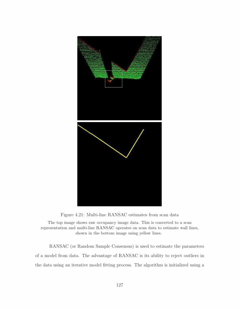
Figure 4.21: Multi-line RANSAC estimates from scan data

The top image shows raw occupancy image data. This is converted to a scanrepresentation and multi-line RANSAC operates on scan data to estimate wall lines,

shown in the bottom image using yellow lines.

RANSAC (or Random Sample Consensus) is used to estimate the parameters

of a model from data. The advantage of RANSAC is its ability to reject outliers in

the data using an iterative model fitting process. The algorithm is initialized using a

127

minimum, random set of points required to estimate the initial model parameter set,

which in this case is the slope-intercept pair (m, c) from the standard line equation

y = mx + c. Following this, other points from the data set which fit the initial

model with an acceptable error are added to a set called the consensus set. Least

squares line fitting is then used to revise the parameters of the initial line equation.

The cumulative reprojection error of the model is then estimated using the revised

parameter set.

The above process is repeated an arbitrary number of times, though it is

possible to estimate an upper limit on the number of iterations required to find an

acceptable parameter set, provided one exists [107]. The seed points used for initial

parameter estimation are randomly chosen for each iteration, which gives this algo-

rithm the randomness necessary to improve the chances of finding the a representative

parameter set. Parameter sets and cumulative errors from all iterations are stored,

and the lowest error set is chosen as being the desired line equation.

A single RANSAC run explained in the preceding paragraphs yields one of

the many wall lines which may be available in the raw (scan) data. To get the rest

of the lines, it is necessary to run RANSAC multiple times. For each run, the set

of available points is pared down to the ones yet to be included in a consensus set.

When a sufficiently large fraction of the total number of points has been included in

one line or another, the multi-RANSAC loop terminates.

Each of the above constituent parts of multi-line RANSAC is expanded in

the rest of this section. Steps (A)-(F) are iteratively carried out until a termination

condition is satisfied.

A) Initialize the set of scan points Si = (rp, θp), p = 1 . . .Ni, i = 0 using the

techniques from Section 4.3.3.

B) Estimate a RANSAC line using the revised set of scan points Si. Mul-

128

tiple estimates are found from Step (1)-(8) and the best of these is considered to be

the RANSAC line for the ith iteration.

1) For the current jth iteration, initialize the consensus set to an empty

set, Cj = φ.

2) Randomly select two points pt0Siand pt1Si

from the set Si. If the points

are too close to each other or too far apart, select a different pair of points. This

modification to the standard RANSAC implementation is necessary to filter out wall

line detections which are either too short or too long. Add the two points to the

consensus set Cj .

3) Estimate the initial line parameters (minitj , cinitj ). If the line is vertical,

these parameters come from the model x = minitj y + cinitj . Otherwise, the model to

be estimated is y = minitj x+ cinitj .

4) Build the consensus set using the initial model. For each point ptpSi, p =

1 . . .Ni in the set Si,

• Find the reprojected point ptpj .

• Calculate the reprojection error in pixels, errpj =∥

∥ptpj − ptpj∥

∥.

• If the error is below a threshold, errpj < errinitmax, add ptpj to consensus set Cj.

From experimental data, it was found that a strict threshold of errinitmax = 5 pixels

worked best for our data.

5)Check the inlier ratio for the consensus set Cj. Let the consensus set have

Mj points. Then the inlier ratio is given by ratioinlierj =Mj

Ni. Based on the inlier ratio,

make a decision about continuing or skipping this iteration. If ratioinlierj < ratiominj ,

return to Step B(1). Since multiple wall lines might be visible to the sensor, this

threshold is set to a rather low value of ratiominj = 0.2, i.e. 20% of points in Ni need

to satisfy this line parameter estimate to proceed with the remaining steps.

129

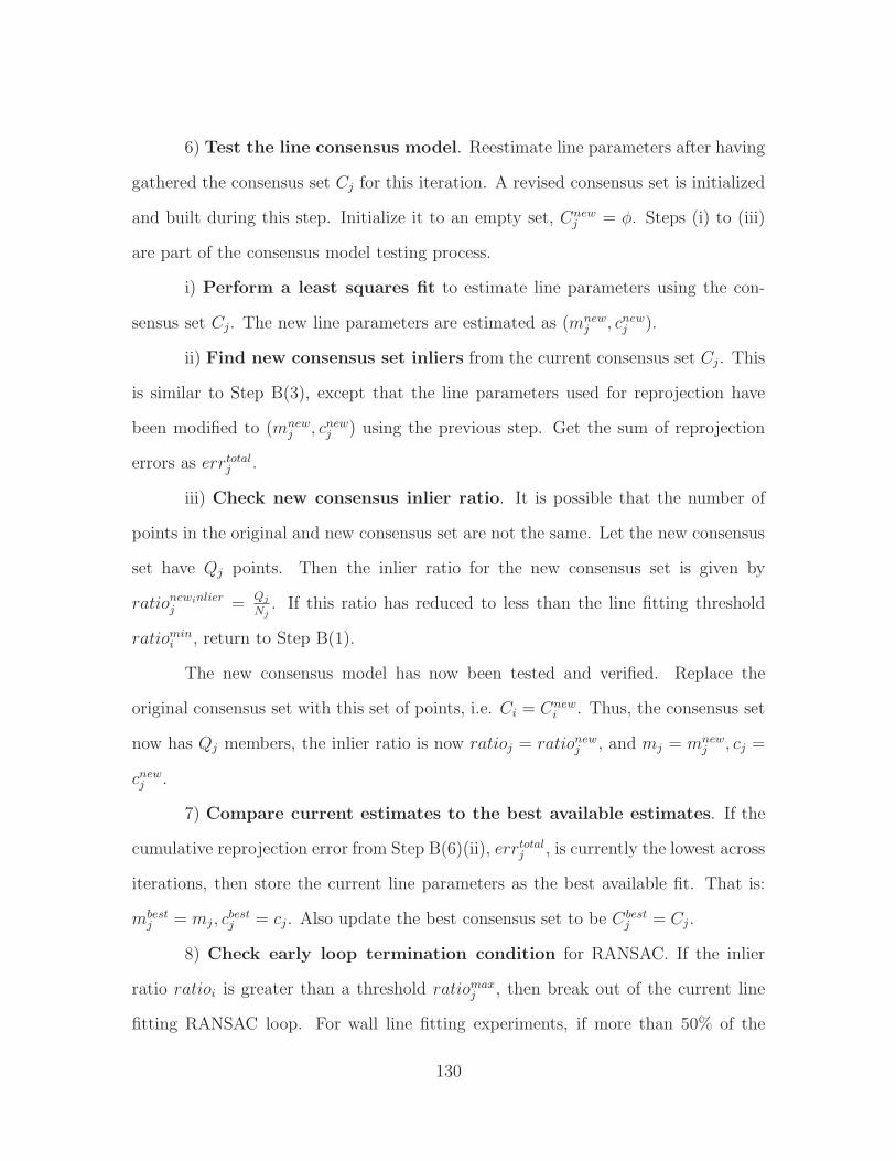
6) Test the line consensus model. Reestimate line parameters after having

gathered the consensus set Cj for this iteration. A revised consensus set is initialized

and built during this step. Initialize it to an empty set, Cnewj = φ. Steps (i) to (iii)

are part of the consensus model testing process.

i) Perform a least squares fit to estimate line parameters using the con-

sensus set Cj. The new line parameters are estimated as (mnewj , cnewj ).

ii) Find new consensus set inliers from the current consensus set Cj. This

is similar to Step B(3), except that the line parameters used for reprojection have

been modified to (mnewj , cnewj ) using the previous step. Get the sum of reprojection

errors as errtotalj .

iii) Check new consensus inlier ratio. It is possible that the number of

points in the original and new consensus set are not the same. Let the new consensus

set have Qj points. Then the inlier ratio for the new consensus set is given by

rationewinlierj =

Qj

Nj. If this ratio has reduced to less than the line fitting threshold

ratiomini , return to Step B(1).

The new consensus model has now been tested and verified. Replace the

original consensus set with this set of points, i.e. Ci = Cnewi . Thus, the consensus set

now has Qj members, the inlier ratio is now ratioj = rationewj , and mj = mnewj , cj =

cnewj .

7) Compare current estimates to the best available estimates. If the

cumulative reprojection error from Step B(6)(ii), errtotalj , is currently the lowest across

iterations, then store the current line parameters as the best available fit. That is:

mbestj = mj , c

bestj = cj. Also update the best consensus set to be Cbest

j = Cj .

8) Check early loop termination condition for RANSAC. If the inlier

ratio ratioi is greater than a threshold ratiomaxj , then break out of the current line

fitting RANSAC loop. For wall line fitting experiments, if more than 50% of the

130

points in the set Si were assigned to a line, ratiomaxj = 0.5, then the current line was

declared a good estimate. If enough iterations have been run, exit the RANSAC loop.

The maximum number of iterations for this experiment was jmax = 250. If neither of

the previous stopping conditions is satisfied, return to Step (B)(1).

C) Get properties of the RANSAC line. Using the best line estimate

from Steps B(1)-B(8), calculate properties of the RANSAC line which will be useful

for the rotation estimate:

• Extreme points of the line.

• Length of the line.

• Angle of the line with respect to the image x axis.

D) Reduce the set of points available for the next line estimate. Elements

of the best consensus set Cbestj are removed from the scan points set Si. If the

best consensus set contained M bestj points, then the revised scan points set contains

Ni = Ni −M bestj elements.

E) Check scan point termination condition. The ratio of points currently

assigned to one of the lines is given by ratioscani = N0−Ni

N0. If enough points have been

assigned to one of the lines, i.e. ratioscani > ratioscanmax , then terminate multi-line

RANSAC. This termination value was set at ratioscanmax = 0.8, i.e. 80% points have

been assigned to one of the lines. If enough iterations have been run, imax = 100 in

this case, then terminate multi-line RANSAC. If neither of the previous conditions is

satisfied, return to Step (B).

The output of multi-line RANSAC is a set of lines which are representative of

the wall lines in the hallway. This set, along with additional line properties computed

in Step (C) of the above algorithm, facilitates estimating Manhattan rotation as

131

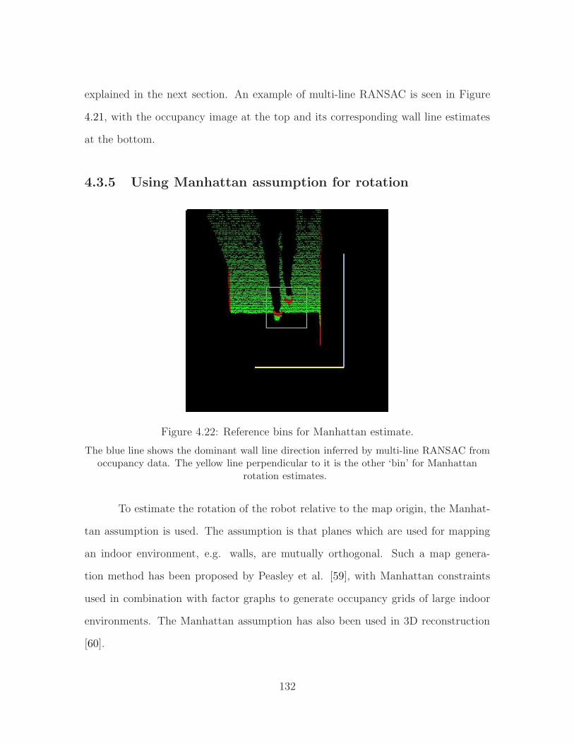
explained in the next section. An example of multi-line RANSAC is seen in Figure

4.21, with the occupancy image at the top and its corresponding wall line estimates

at the bottom.

4.3.5 Using Manhattan assumption for rotation

Figure 4.22: Reference bins for Manhattan estimate.

The blue line shows the dominant wall line direction inferred by multi-line RANSAC fromoccupancy data. The yellow line perpendicular to it is the other ‘bin’ for Manhattan

rotation estimates.

To estimate the rotation of the robot relative to the map origin, the Manhat-

tan assumption is used. The assumption is that planes which are used for mapping

an indoor environment, e.g. walls, are mutually orthogonal. Such a map genera-

tion method has been proposed by Peasley et al. [59], with Manhattan constraints

used in combination with factor graphs to generate occupancy grids of large indoor

environments. The Manhattan assumption has also been used in 3D reconstruction

[60].

132

Making this assumption is an effort to find a drift-free rotation estimation

method in mapping. An overview of SLAM and standard SLAM techniques was pre-

sented in a tutorial by Durrant-Whyte and Bailey [51, 52]. In conventional SLAM

techniques, 3D correspondence between frames is used as the basis for estimating

inter-frame translation and rotation. Such correspondence can be obtained using 3D

point cloud data directly and establishing correspondences between 3D features [103],

or combining 2D feature matching (e.g. joint Lucas-Kanade [99]) with depth data

from RGB-D sensors, or performing scan matching between the polar scan representa-

tions of successive frames [57]. However, these techniques rely on accurate inter-frame

rotation estimates to be effective for mapping. One poor set of correspondences can

throw the map off completely or introduce a rotational drift which accumulates over

time.

An effective way to counter inter-frame drift due to correspondence errors is

to take point correspondences completely out of the picture and replace them with

another type of feature which is most commonly found in the mapping environment.

The presence of wall lines is one such feature for indoor environments. As explained

in the previous section, RANSAC provides a set of line estimates for wall lines in any

given occupancy image.

To apply the Manhattan assumption, wall lines found in the initialization

frame of the map used to get the reference line for rotation. This is done by taking

the median of all the line orientations detected in multi-line RANSAC. Since me-

dian orientations for subsequent lines belong to planes which are either parallel or

perpendicular to the reference orientation, Manhattan rotation is estimated as the

difference between any given median orientation and the initial orientation. This

process is explained ahead in detail.

Consider Figure 4.22. The blue line is the line detected by RANSAC in the

133

Figure 4.23: Sample mapping frame for Manhattan estimate.

The gray line in this image is the estimated RANSAC line. This is compared with theinitialization map RANSAC lines to ultimately give inter-frame and total rotation for

mapping.

initialization or reference frame, frame 0. Let θa0 be the angle of this line with the

horizontal. Another ‘bin’ is created for the purpose of matching future line detections

to this reference line. Let θb0 = θa0 + 90◦ be the value of this bin, represented by the

yellow line in the figure.

Consider, for example, a subsequent frame n in the mapping trial in Figure

4.23. Let the orientation of the median line with respect to the horizontal be θn.

Suppose the median RANSAC line (shown in gray in the image) is orthogonal with

respect to the reference line from Figure 4.22. This could mean one of two things:

• The robot has rotated nearly 90◦ relative to its initial pose, or

• There is a wall ahead of the robot which is perpendicular to the wall observed

in the initial frame.

To disambiguate these conditions, θn0 is always chosen as the minimum of |θn − θa0 |

134

and |θn − θb0 | . Inter frame rotation is measured as θnn−1 = θn0 − θn−10 . The total rota-

tion of the robot relative to its initial pose, for frame n is then recursively determined

as

θntotal= θn−1total + θnn−1 (4.2)

. The creation of orthogonal bins thus helps in resolving the ambiguity in Manhattan

estimation.

Thus, the process of scan generation, multi-line RANSAC, and Manhattan

rotation estimation result in an estimate of the rotation of the robot relative to its

initial pose.

4.3.6 Approximating translation using dead reckoning

To map data from the current scan to the composite map of the environment,

translation estimate relative to the map initialization frame is required. Since the

robot is translating in the (x, z) plane, let the two translation estimates be represented

by (xntotal, yntotal

), where

xntotal= xn−1total +∆xn

n−1

zntotal= zn−1total +∆znn−1

(4.3)

where ∆xnn−1 and ∆znn−1 are inter-frame translations along x and z axis, respectively.

In the absence of reliable translation estimates from visual odometry and point

cloud matching techniques, the motion pattern of the robot is used to estimate inter-

frame translations. While following a leader, the robot first aligns itself with the

leader by rotating to the observed leader angular offset, and then translates with a

fixed velocity along this vector. Translation continues until the next motion command

is received based on the leader’s new position. This process of stop-rotate-translate

135

is designed to give the mapping system enough information to estimate inter-frame

translation.

Let ∆tnn−1 be the time elapsed since the last translation estimate. From the

motion algorithm, we know that the robot has been commanded to translate at a

known velocity, represented by rnn−1. Then the distance traveled by the robot between

frames is given by

rnn−1 = rnn−1 ·∆tnn−1 (4.4)

To get the total translation of the robot (relative to map origin), the radial

translation in Eqn. 4.4 has to be expressed in terms of its Cartesian components.

Using Eqn. 4.2, these components can be expressed as follows:

∆xnn−1 = cos(θntotal

) · rnn−1

∆znn−1 = sin(θntotal) · rnn−1

Thus, all the terms in Eqn. 4.3 have been determined and the translation of

the current frame relative to the map initialization frame has been calculated. All

data required to build and update the map is available.

4.3.7 Map building and output

The map is generated as a square image of arbitrary size, with the scale of

1 pixel = 10 mm along each image axis. Thus, a 1600×1600 image covers a mapping

area of 16× 16 meters, which is substantial in terms of its applicability to the person

following problem.

The occupancy image generated in Section 4.3.2 has been converted to a scan

representation using the method in Section 4.3.3. The coordinates of each of these

scan points are transformed to global coordinates. Let the scan point for frame i

136

Figure 4.24: Map output down a straight hallway.

Occupancy images, a sample of which is shown in the top panel, are stitched togetherusing the mapping algorithm to yield the map image. Red pixels in the map image are

aligned scan points from the first to the current frame, and yellow dots show the motion ofthe robot down the straight hallway. The white rectangle is the position of the leader in

the current frame.

be at an angle θi relative to the robot position during that frame. Let ri be the

radial distance between the point location and the robot location in the (x, z) plane.

Then, using the total rotation and translation estimates from Eqn. 4.2 and Eqn. 4.3

137

respectively, the scan point is situated on the map at:

xintotal= xntotal

+ cos(θntotal) · ri

zintotal= zntotal

+ sin(θntotal) · ri

(4.5)

Figure 4.25: Map output at a L-junction.

The layout and characteristic features in this figure are identical to Figure 4.24. Yellowdots show the motion of the robot as it turns around the L-shaped hallway.

138

The map is reset when one or more of the following conditions are satisfied:

1. No RANSAC line estimate could be found for the given frame.

2. Leader is close to one of the edges of the map image.

3. Leader position is inferred to be on one of the ‘occupied’ map pixels.

4. Robot position is inferred to be on one of the ‘occupied’ map pixels.

While the last two conditions are obvious indicators that something has gone wrong

with the mapping output, the second condition is simply a map reset triggered by

the range of the map. For the practical Level-3 follower, a range of 16 × 16 meters

was found to be sufficient, however, there may be environments in which a larger

map may be required. Alternately, it should be possible to completly eliminate range

resets by discarding older positional information and shifting the entire map up-down

or left-right using a shifting logic appropriate for the application. A logical resolution

of the first reset condition remains elusive. Since rotation and translation estimates

both rely on good Manhattan estimates, a RANSAC failure propagates all the way

to the final output. Hence, RANSAC failures mandate a map reset.

The output of the map for three typical hallway configurations is shown in a

Figures 4.24, 4.25, and 4.26. In all of these figures, the four images at the top are

occupancy maps at various interesting or representative stage in map building. The

image at the bottom of each figure shows the final map output, with the white box

in the figure showing leader position in the final frame and yellow squares showing

the position of the robot as it followed the leader during the trial.

In Figure 4.24, the robot follows a leader down a straight passage. The fact

that door frames seen in the occupancy image neatly overlap in the map output is

indicative of the translation estimate being accurate. In case of poor translation

139

Figure 4.26: Map output at a T-junction.

The layout and characteristic features in this figure are identical to Figure 4.24. Yellowdots show the motion of the robot as it turns around the T-shaped hallway.

estimates, the overlap for such features in the environment is poor. In Figure 4.25,

the robot follows the leader around a L-junction after a long straight route in the

initial part of the trial. Performance over both the straight section (as seen by the

alignment for the door frame on the left side of the map image) and around the corner

140

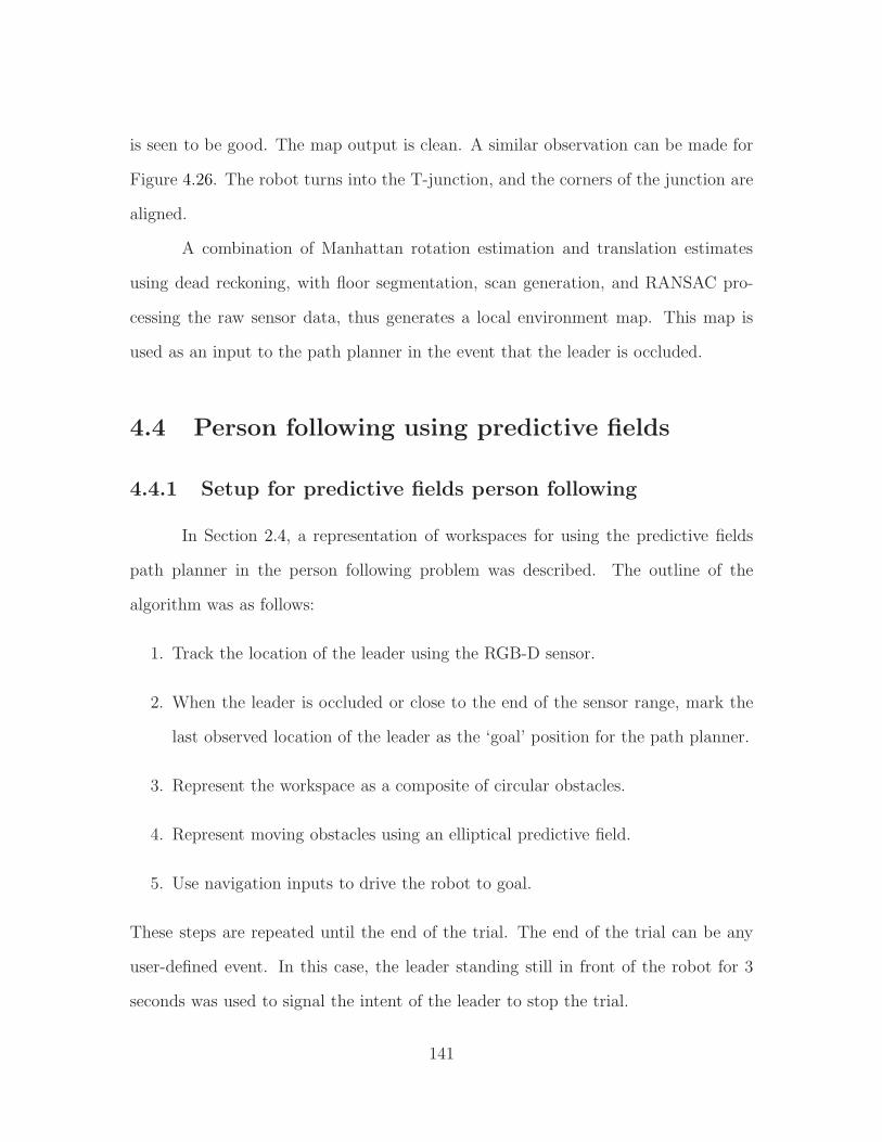
is seen to be good. The map output is clean. A similar observation can be made for

Figure 4.26. The robot turns into the T-junction, and the corners of the junction are

aligned.

A combination of Manhattan rotation estimation and translation estimates

using dead reckoning, with floor segmentation, scan generation, and RANSAC pro-

cessing the raw sensor data, thus generates a local environment map. This map is

used as an input to the path planner in the event that the leader is occluded.

4.4 Person following using predictive fields

4.4.1 Setup for predictive fields person following

In Section 2.4, a representation of workspaces for using the predictive fields

path planner in the person following problem was described. The outline of the

algorithm was as follows:

1. Track the location of the leader using the RGB-D sensor.

2. When the leader is occluded or close to the end of the sensor range, mark the

last observed location of the leader as the ‘goal’ position for the path planner.

3. Represent the workspace as a composite of circular obstacles.

4. Represent moving obstacles using an elliptical predictive field.

5. Use navigation inputs to drive the robot to goal.

These steps are repeated until the end of the trial. The end of the trial can be any

user-defined event. In this case, the leader standing still in front of the robot for 3

seconds was used to signal the intent of the leader to stop the trial.

141

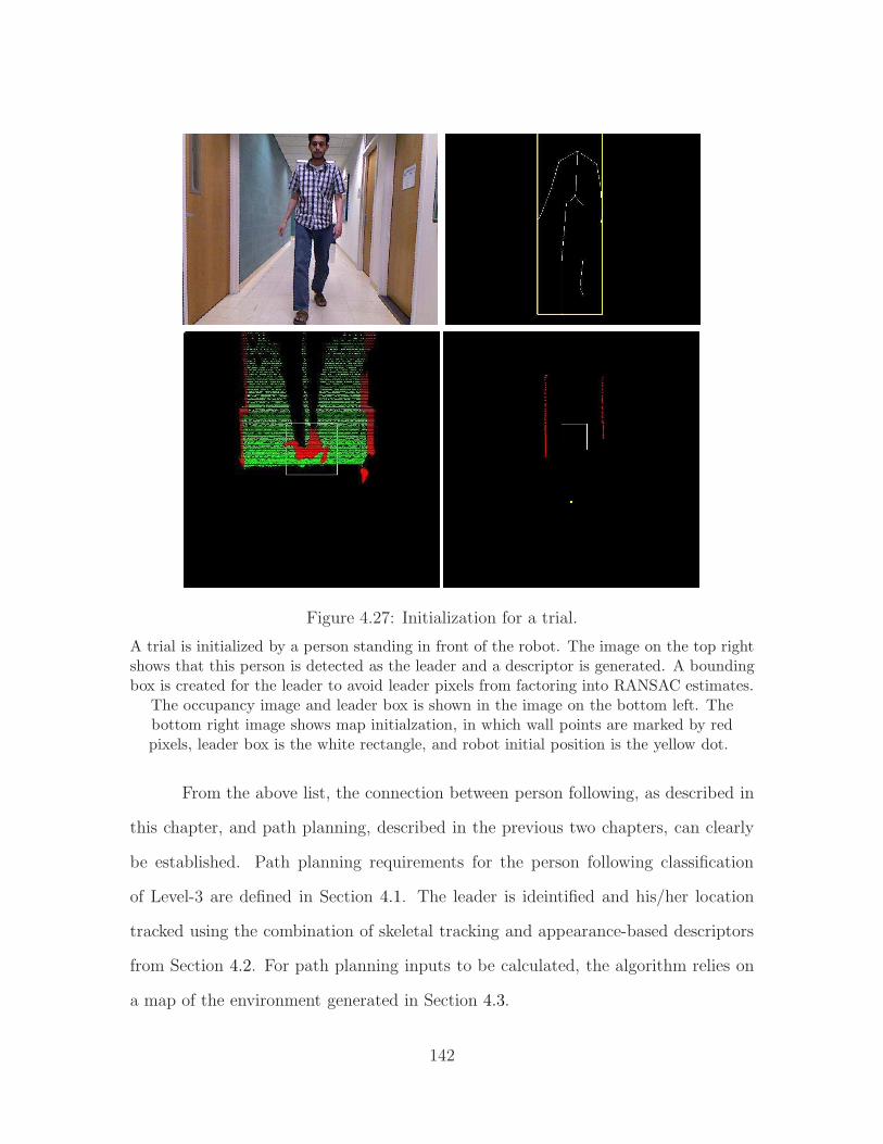
Figure 4.27: Initialization for a trial.

A trial is initialized by a person standing in front of the robot. The image on the top rightshows that this person is detected as the leader and a descriptor is generated. A boundingbox is created for the leader to avoid leader pixels from factoring into RANSAC estimates.

The occupancy image and leader box is shown in the image on the bottom left. Thebottom right image shows map initialzation, in which wall points are marked by redpixels, leader box is the white rectangle, and robot initial position is the yellow dot.

From the above list, the connection between person following, as described in

this chapter, and path planning, described in the previous two chapters, can clearly

be established. Path planning requirements for the person following classification

of Level-3 are defined in Section 4.1. The leader is ideintified and his/her location

tracked using the combination of skeletal tracking and appearance-based descriptors

from Section 4.2. For path planning inputs to be calculated, the algorithm relies on

a map of the environment generated in Section 4.3.

142

The setup for the use of path planning integrated with person following is as

follows. A forward-looking Kinect sensor is mount on a tripod on a Pioneer P3-AT

robot. Both the Kinect and Pioneer are interfaced with the laptop sitting at the

back of the Pioneer. As a calibration step, the floor plane may be established by the

user using the procedure from Section 3.3.1. A floor plane threshold of 3.5 was found

to be acceptable for the forward-looking sensor. An experimental trial begins with

the leader standing in front of the robot. When the skeletal tracker has detected the

person, a leader descriptor is generated and used as the person identification reference

for the rest of the trial. Initialization data for a typical trial is shown in Figure 4.27.

4.4.2 Person following strategy - exact following and path

planning

The robot attempts to follow the leader ‘exactly’ as long as the leader is visible.

This means that the control input to the robot is similar to a proportional control

input with saturation, i.e.

r = min(robserved − rdesired, rmax)

θ = θobserved − θdesired

where (robserved, θobserved) are polar coordinates of the leader with respect to the

robot. The desired straight line distance to the leader is given by rdesired and the

leader should ideally be at the center of the Kinect’s field of view, i.e. θdesired = 90◦.

Translation and rotation inputs are in mm/sec and degrees/sec respectively.

When the leader is occluded or moves out of sensor range, the leader following

module switches to the path planner. As explained in Section 4.1, Level-3 following

requires a ‘patient leader’, i.e. someone who waits for the robot to overcome occlusions

143

Figure 4.28: Transition from exact following to path planning.

When the leader moves out of sensor range or is occluded, the path planner gets activated.In the image on the left, the leader (white rectangle) is about to move out of sensor rangerelative to the robot (yellow dots). This activates the path planner. Adjacent circles along

the red pixels are wall obstacles. The small circle around the last yellow dot from theimage on the left is the robot initial position, with blue and white lines indicating actualand desired heading as per navigation inputs. The small dot at the top of the workspace is

the leader position, and the green circle around it is the stopping radius around theleader, fixed by the minimum sensing distance for the Kinect. If the robot reaches the

border of this circle, navigation stops and robot waits to reacquire the leader.

or environmental obstacles during the trial. So the underlying assumption is that the

leader waits, or at least does not move a great distance relative to the position where

he/she was ‘lost’ to the robot. The switch from exact following to path planning

requires the robot’s environment to be characterized using circular envelopes in the

manner described in Section 2.4.

To get this representation, the goal position is identified as the last observed

location of the leader relative to the local map. Robot initial position is the current

position of the robot relative to the map. To get obstacle positions, the map image

is divided into a grid of m × n square cells. The number of red pixels, signifying an

occupied pixel location in the map, in each cell is counted. If this number is above

144

a threshold, then a wall obstacle is assigned to that cell, with the same diameter as

the width of the cell. The workspace envelope is placed at the central point between

robot initial position and goal position. Its radius is assigned to be the distance to

the robot (or goal) plus a padding value to ensure that the robot does not start close

to the workspace boundary.

The output of this process is seen in Figure 4.28. The image on the left shows

the point in the trial where the leader is about to move out of robot sensor range.

This triggers the path planning mode of operation, and the workspace representation

is generated as shown in the image on the right. Walls are seen to be enveloped with

orange circles, designating the detected obstacles for the path planner. Yellow dots

show the path taken by the robot in previous frames, and the initial position of the

robot is marked by the yellow dot with a circle drawn around it. There are two lines

overlaid on this robot circle. The goal position is marked by a small rectangle near

the top of the workspace envelope.

4.4.3 Experimental results for path planning

The performance of the predictive fields path planner is demonstrated using

three typical scenarios:

• Robot overcomes sensor range occlusion in the presence of environmental ob-

stacles.

• Robot overcomes sensor range occlusion in the presence of a stationary human

in the workspace.

• Robot overcomes moving obstacle occlusion, where the moving obstacle is an-

other human in the workspace.

145

Figure 4.29: Path planning to overcome sensor range occlusion.

Example of sensor range occlusion recovery. The significance of the features in the map isexplained in Figure 4.28. Overlapping white circles show the path of the robot to the last

observed leader position.

The description of Figure 4.28 is completed by commenting on objects in

the image which represent run-time events. The blue line is the observed heading

of the robot, from Manhattan rotation estimates, and the white line is the desired

heading. Another circle has been added to the representation and that is the circle

drawn around the goal position. If the robot is within this circle and the leader has

been reidentified, then the path planner switches off and the ‘exact following’ mode

resumes. In every case, the trial stops after the leader is stationary for a few seconds.

146

The navigation method for the robot to move to goal is described as follows.

On establishing the workspace configuration, the path planner returns a directional

vector as the velocity input to the robot. This is converted to a heading in degrees.

The current heading of the robot is estimated using the scan data - RANSAC -

Manhattan rotation system. The robot is rotated gradually to its desired heading

(to allow for a more accurate inter-frame Manhattan estimate) and then translated

for a fixed period of time at a fixed velocity along this new orientation. This process

continues until the robot has converged to goal.

Figure 4.29 shows the path planning-based recovery from sensor range occlu-

sion of the leader. In this type of occlusion, the leader travels beyond the sensor range

of the Kinect (4000mm) and the robot has to go to the last observed leader location

to recover from this event. Small overlapping circles in the image show the path

taken by the robot from the time the leader has been occluded to the time it is close

enough to be able to reidentify the leader. If the leader has, once again, moved out

of sensor range of the Kinect, the robot waits at the goal position and it is expected

that the leader will return to the Kinect’s field of view to allow a resumption of the

person following activity. The last requirement is appropriate for the ‘patient leader’

scenario.

Figure 4.30 shows an example of the robot planning a path in the case of

sensor range occlusion with the leader and another individual. The image to the

left shows the robot leader and another person in the field of view of the Kinect.

Eventually, the leader (standing to the right) moves out of sensor range. In keeping

with the occlusion recovery method, the algorithm first tries to match the descriptor

of the person still in sensor range, and an inadequate match score triggers the path

planning method for occlusion recovery. Wall obstacles are identified using the grid

method, and the detected, non-leader person is labeled as a potential moving obstacle

147

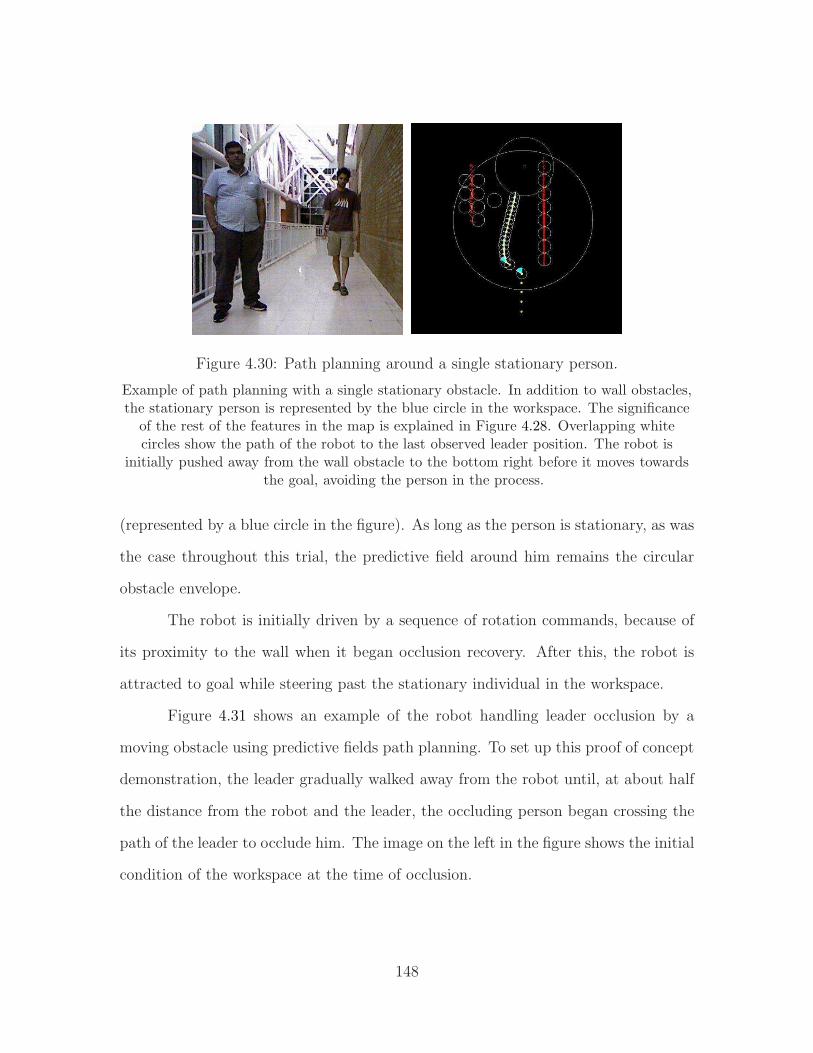
Figure 4.30: Path planning around a single stationary person.

Example of path planning with a single stationary obstacle. In addition to wall obstacles,the stationary person is represented by the blue circle in the workspace. The significance

of the rest of the features in the map is explained in Figure 4.28. Overlapping whitecircles show the path of the robot to the last observed leader position. The robot is

initially pushed away from the wall obstacle to the bottom right before it moves towardsthe goal, avoiding the person in the process.

(represented by a blue circle in the figure). As long as the person is stationary, as was

the case throughout this trial, the predictive field around him remains the circular

obstacle envelope.

The robot is initially driven by a sequence of rotation commands, because of

its proximity to the wall when it began occlusion recovery. After this, the robot is

attracted to goal while steering past the stationary individual in the workspace.

Figure 4.31 shows an example of the robot handling leader occlusion by a

moving obstacle using predictive fields path planning. To set up this proof of concept

demonstration, the leader gradually walked away from the robot until, at about half

the distance from the robot and the leader, the occluding person began crossing the

path of the leader to occlude him. The image on the left in the figure shows the initial

condition of the workspace at the time of occlusion.

148

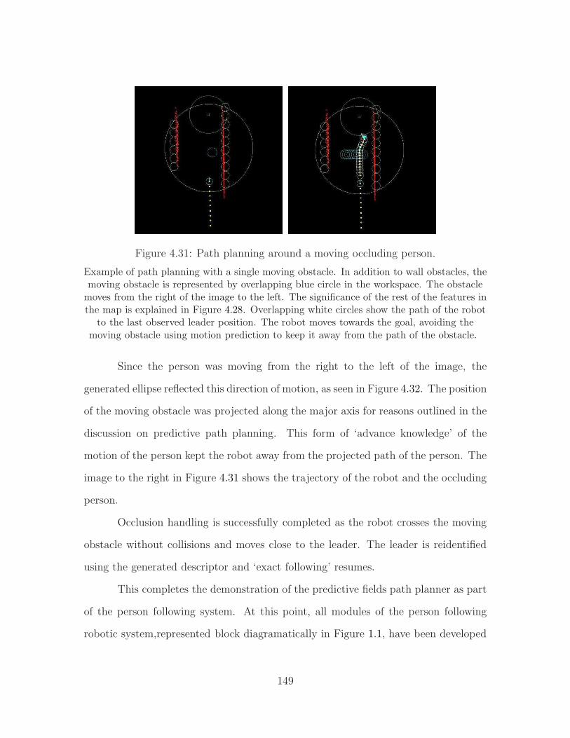
Figure 4.31: Path planning around a moving occluding person.

Example of path planning with a single moving obstacle. In addition to wall obstacles, themoving obstacle is represented by overlapping blue circle in the workspace. The obstaclemoves from the right of the image to the left. The significance of the rest of the features inthe map is explained in Figure 4.28. Overlapping white circles show the path of the robot

to the last observed leader position. The robot moves towards the goal, avoiding themoving obstacle using motion prediction to keep it away from the path of the obstacle.

Since the person was moving from the right to the left of the image, the

generated ellipse reflected this direction of motion, as seen in Figure 4.32. The position

of the moving obstacle was projected along the major axis for reasons outlined in the

discussion on predictive path planning. This form of ‘advance knowledge’ of the

motion of the person kept the robot away from the projected path of the person. The

image to the right in Figure 4.31 shows the trajectory of the robot and the occluding

person.

Occlusion handling is successfully completed as the robot crosses the moving

obstacle without collisions and moves close to the leader. The leader is reidentified

using the generated descriptor and ‘exact following’ resumes.

This completes the demonstration of the predictive fields path planner as part

of the person following system. At this point, all modules of the person following

robotic system,represented block diagramatically in Figure 1.1, have been developed

149

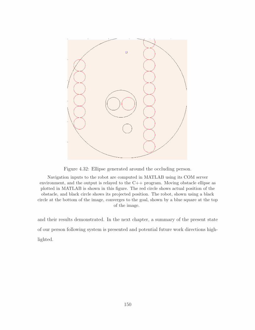
Figure 4.32: Ellipse generated around the occluding person.

Navigation inputs to the robot are computed in MATLAB using its COM serverenvironment, and the output is relayed to the C++ program. Moving obstacle ellipse asplotted in MATLAB is shown in this figure. The red circle shows actual position of theobstacle, and black circle shows its projected position. The robot, shown using a black

circle at the bottom of the image, converges to the goal, shown by a blue square at the topof the image.

and their results demonstrated. In the next chapter, a summary of the present state

of our person following system is presented and potential future work directions high-

lighted.

150

Chapter 5

Conclusions and future work

The goal of the work presented here was the development of a robotic person

follower capable of identifying its leader, handling leader occlusions, generating a map

of its local environment, and navigating to its a position relative to the leader by using

a combination of ‘exact following’ and path planning. In this chapter, the technical

contributions made are reviewed and future research directions are discussed.

5.1 Conclusions

Person follower systems in described in literature have been either explicitly

or implicitly defined in terms of the capabilities of the robot follower. The role of

the human, central to this human-robot interaction system, has not been defined. In

the work here, a novel human leader-based classification system for person

followers was developed (Section 4.1). This classification system identifies four

levels of expected leadership: ‘Level 1’ or ‘Fully cooperative leader’, ‘Level 2’ or ‘Par-

tially cooperative leader’, ‘Level 3’ or ‘Patient leader’, and ‘Level 4’ or ‘Independent

leader’. Contemporary person followers were classified with the system to illustrate

151

how the system can be used to identify the similarities and differences between dis-

parate robotic systems. Such a system may be useful to identify the robot ‘class’

when service robots with a strong or central person following component become

commercially viable.

The work proposed here best fits the ‘Level 3’ follower classification. For

Level 3 systems, occlusion handling is mandated, and an occlusion detection and

recovery algorithm was developed (Section 4.2) for this purpose. This algorithm

is based on building an appearance descriptor around the reliable and robust Kinect

skeletal tracker. Skeletal information from the tracker is augmented with a descriptor

based on HSI and L*a*b* (CIE 1976) color spaces to create a leader descriptor. After

the leader descriptor is generated, descriptors in subsequent frames are compared to

infer and handle occlusions. It was found that the generated descriptor was sufficiently

discriminative and the robotic follower was consistently able to identify its leader and

infer occlusions.

To follow a person around occlusions, the robot needs to localize itself in its

environment. To enable this, a simple mapping approach was developed (Sec-

tion 4.3). This localization is achieved using a combination of multi-line RANSAC,

Manhattan rotation estimates, and dead reckoning odometry. Low-drift local maps

were generated as a result, and it was found that a good RANSAC implementation

was central to the consistent performance of the system. The combination of these

elements yields an improved approach to generate low-drift maps using low-cost, off-

the-shelf sensors.

The local map serves as input to the path planning module. The navigation

function path planner was chosen for its mathematical rigor and modified to develop

a path planner sensitive to obstacle motion (Section 2.2). This path planner,

called the predictive fields path planner, uses an elliptical envelope to represent the

152

predicted motion of obstacles. The repulsive field generated by such a representation

drives the robot away from the path of danger, i.e. away from the predicted paths

of obstacles. The concept of danger was quantified using a metric called the ‘risk

score’, and it was shown that using the motion encoding ellipse generates a lower risk

score than the no-ellipse case for a variety of typical scenarios. This work represents

a significant enhancement to the static navigation function approach as it facilitates

path planning in more realistic, dynamic environments.

To guide the robot to goal, a method to generate practical control in-

puts to the robot is developed (Section 2.3). Navigation function path planning

resulted in unpredictably high control inputs and extremely sensitive gain parameters.

It was shown that using a normalized control input, used by predictive fields path

planners, resulted in a stable system; moreover, normalized inputs (in the magnitude

range [−1 . . . 1]) could be interpreted as direction inputs which could easily be fol-

lowed by the robotic system. Experimental and simulation implementations confirm

this feature of the control method.

To apply the controller in a practical environment, a method to implement

predictive fields in practical workspaces was developed (Section 2.4). This

representation obviated the need for the special ‘star-world’ transformation required

by navigation functions for the robot to operate in practical worlds. This representa-

tion also included leader waypoint generation method which makes it possible for the

path planner to navigate in highly dynamic workspaces where the robot, obstacles,

and goal may all be simultaneously in motion. Simulation results corroborate the

utility of the workspace representation and the path planning technique in general.

Finally, an experimental verification of predictive fields path planning

was provided (Chapter 3). This is one of the first experimental demonstrations of

navigation functions in literature. Navigation functions, though widely cited for their

153

formulation and mathematical properties, have rarely been used in mobile robot ex-

periments. Various prohibiting factors were discussed in previous points. However,

after overcoming these limitations with the modified approach, it was possible to

demonstrate both navigation functions and predictive fields in an experimental setup.

Two types of experiments were conducted. The first used a combination of the Kinect

and iRobot Roomba; the second was the demonstration of predictive fields navigation

in the framework of the person follower (Section 4.4.3). This is compelling demon-

stration of navigation functions in everday environments using standard sensors and

robots and it is hoped that this encourages more widespread experimental develop-

ment of this classic path planning technique.

Thus, a complete robotic system to follow a person around occlusions in indoor

environments using path planning was designed and experimentally demonstrated.

5.2 Future work

Possible future directions for the work described here are:

• Develop benchmarks to augment the person follower classification

system. The classification system, in its present form, is a handy guideline for

expected human-robot interaction for a given person follower. However, this

system, and the area of service robotics research in general, does not have a set

of benchmarks against which the performance of a follower could be measured.

For example, though it is possible to categorize a system as a ‘Level 3’ follower,

there is no way of comparing one ‘Level 3’ system with any other. Thus, the

question of quality of a person follower has only subjective explanations.

• Develop a leader model using additional modalities to supplement

154

the appearance model. The leader appearance model, even with its use of

robust color spaces for descriptor generation, has a known failure case when

two persons wearing a similar set of clothes occlude each other and reemerge

in front of the robot. The robot begins to follow the wrong person in such a

case. For certain applications, e.g. hospital assistants for doctors, such a failure

case cannot be tolerated. Hence, other identification modalities, such as face

recoginition or RFID tags or gait recognition, could be investigated as additions

to the existing leader tracking and occlusion handling framework.

• Develop various geometries for predictive fields. Predictive fields used

in our work have all been elliptical, since directionality and speed of obstacle

motion are captured well by an elliptical envelope. However, it might be inter-

esting to create different motion models for different types of moving obstacles,

e.g. humans, carts, other robots, and develop predictive field geometries specific

to each type of motion.

• Develop a path planner with minimal tuning requirements. Even with

improved workspace and obstacle representation and practical control inputs,

the current system requires its navigation gain to be tuned for the robot to

converge. Were this requirement to be relaxed, either by learning tuned values

over many trials, or by an iterative method such as the one suggested by Filip-

pidis [77], the setup time and effort to run an experiment in a new environment

would be greatly reduced.

• Develop an application specific person following system. Our person

follower was developed as a generic solution for various facets of the problem.

However, a specific application such as ‘hospital assistant’ or ‘grocery cart’ will

introduce a set of specific design requirements. Such design specifications will,

155

in turn, define additional modules, e.g. speech recognition, telepresence, which

will bring the system closer to its intended goal of assisting people in everyday

environments.

• Develop event detection modules to improve navigation behavior.

Since our person follower operates in indoor hallways, its navigation behav-

ior could improve with an ability to detect events which are common to such

environments. For example, detecting events such as a door being opened will

allow the robot to anticipate the introduction of an obstacle into the workspace,

and even in the absence of the physical obstacle, plan a path which takes it away

from the door.

In summary, the person following problem provides an interesting set of chal-

lenges in terms of robot research and development. In the work presented in this

dissertation, methods to address some of these challenges have been developed, and

directions for improvements to our system and to the area of person following in

general have been identified.

156

Bibliography

[1] R. Schraft and G. Schmierer, Service robots: products, scenarios, visions. AK Peters, 2000.

[2] R. Kirby, J. Forlizzi, and R. Simmons, “Natural person-following behavior forsocial robots,” in Proceedings of Human-Robot Interaction, March 2007, pp.17–24.

[3] S. Thrun, M. Beetz, M. Bennewitz, W. Burgard, A. Cremers, F. Dellaert,D. Fox, D. Hahnel, C. Rosenberg, N. Roy, J. Schulte, and D. Schulz, “Prob-abilistic algorithms and the interactive museum tour-guide robot Minerva,”International Journal of Robotics Research, vol. 19, no. 11, pp. 972–999, 2000.

[4] J. Buhmann, W. Burgard, A. Cremers, D. Fox, T. Hofmann, F. Schneider,J. Strikos, and S. Thrun, “The mobile robot Rhino,” AI Magazine, vol. 16,no. 1, 1995.

[5] A. Haasch, S. Hohenner, S. Huwel, M. Kleinehagenbrock, S. Lang, I. Toptsis,G. A. Fink, J. Fritsch, B. Wrede, and G. Sagerer, “Biron - the bielefeld robotcompanion,” in in Proc. Int. Workshop on Advances in Service Robotics, 2004,pp. 27–32.

[6] M. Takahashi, T. Suzuki, H. Shitamoto, T. Moriguchi, and K. Yoshida, “De-veloping a mobile robot for transport applications in the hospital domain,”Robotics and Autonomous Systems, vol. 58, no. 7, pp. 889–899, Jul. 2010.

[7] U. Reiser, C. Connette, J. Fischer, J. Kubacki, A. Bubeck, F. Weisshardt,T. Jacobs, C. Parlitz, M. Hagele, and A. Verl, “Care-o-botR©: creating a productvision for service robot applications by integrating design and technology,” inProceedings of the IEEE Conference on Intelligent Robots and Systems (IROS),2009, pp. 1992–1998.

[8] T. Breuer, G. Giorgana Macedo, R. Hartanto, N. Hochgeschwender, D. Holz,F. Hegger, Z. Jin, C. Mller, J. Paulus, M. Reckhaus, J. lvarez Ruiz, P. Plger,and G. Kraetzschmar, “Johnny: An autonomous service robot for domesticenvironments,” Journal of Intelligent and Robotic Systems, vol. 66, no. 1-2, pp.245–272, 2012.

157

[9] T. Wisspeintner, T. van der Zant, L. Iocchi, and S. Schiffer, “RoboCup@Home:Scientific competition and benchmarking for domestic service robots,” Interac-tion Studies, vol. 10, no. 3, pp. 393–428, 2009.

[10] N. Roy, G. Baltus, D. Fox, F. Gemperle, J. Goetz, T. Hirsch, D. Margaritis,M. Montemerlo, J. Pineau, J. Schulte, and S. Thrun, “Towards personal servicerobots for the elderly,” in Proceedings of the Workshop on Interactive Robotsand Entertainment (WIRE 2000), Pittsburgh, PA, May 2000.

[11] H.-M. Gross, C. Schroter, S. Muller, M. Volkhardt, E. Einhorn, A. Bley, C. Mar-tin, T. Langner, and M. Merten, “Progress in developing a socially assistive mo-bile home robot companion for the elderly with mild cognitive impairment,” inProceedings of the IEEE Conference on Intelligent Robots and Systems (IROS),2011, pp. 2430–2437.

[12] U.S. Dept. of Health and Human Services, “A pro-file of older americans: 2012,” 2012. [Online]. Available:http://www.aoa.gov/Aging Statistics/Profile/index.aspx

[13] A. Tani, G. Endo, E. F. Fukushima, S. Hirose, M. Iribe, and T. Takubo,“Study on a practical robotic follower to support home oxygen therapy patients-development and control of a mobile platform-,” in Proceedings of the IEEEConference on Intelligent Robots and Systems (IROS), sept. 2011, pp. 2423–2429.

[14] K. Kida, “Home oxygen therapy in japan: Clinical application and considera-tions for practical implementation,” Japan Medical Association Journal, vol. 54,pp. 99–104, 2011.

[15] D. Feil-Seifer and M. Mataric, “Defining socially assistive robotics,” in Proceed-ings of the 9th International Conference on Rehabilitation Robotics, 2005, pp.465–468.

[16] T. Yoshimi, M. Nishiyama, T. Sonoura, H. Nakamoto, S. Tokura, H. Sato,F. Ozaki, N. Matsuhira, and H. Mizoguchi, “Development of a person followingrobot with vision based target detection,” in Proceedings of the IEEE Confer-ence on Intelligent Robots and Systems (IROS), 2006, pp. 5286–5291.

[17] Z. Chen and S. T. Birchfield, “Person following with a mobile robot usingbinocular feature-based tracking,” in Proceedings of the IEEE Conference onIntelligent Robots and Systems (IROS), Oct. 2007.

[18] W. han Yun, D. Kim, and J. Lee, “Person following with obstacle avoidancebased on multi-layered mean shift and force field method,” in Proceedings ofthe IEEE International Conference on Systems, Man, and Cybernetics (SMC),oct. 2010, pp. 3813 –3816.

158

[19] J. Miura, J. Satake, M. Chiba, K. Ishikawa, K. Kitajima, and H. Masuzawa,“Development of a person following robot and its experimental evaluation,”in Proceedings of the 11th International Conference on Intelligent AutonomousSystems, 2010, pp. 89–98.

[20] J. Satake and J. Miura, “Robust stereo-based person detection and trackingfor a person following robot,” in ICRA Workshop on Person Detection andTracking, 2009.

[21] X. Ma, C. Hu, X. Dai, and K. Qian, “Sensor integration for person trackingand following with mobile robot,” in Proceedings of the IEEE Conference onIntelligent Robots and Systems (IROS), 2008, pp. 3254–3259.

[22] M. Enzweiler and D. M. Gavrila, “A multilevel mixture-of-experts frameworkfor pedestrian classification,” IEEE Transactions on Image Processing, vol. 20,no. 10, pp. 2967–2979, 2011.

[23] M. Bansal, S.-H. Jung, B. Matei, J. Eledath, and H. S. Sawhney, “A real-timepedestrian detection system based on structure and appearance classification.”in Proceedings of the IEEE International Conference on Robotics and Automa-tion (ICRA), 2010, pp. 903–909.

[24] M. Enzweiler and D. M. Gavrila, “Integrated pedestrian classification and orien-tation estimation,” in Proceedings of the IEEE Conference on Computer Visionand Pattern Recognition (CVPR), 2010, pp. 982–989.

[25] M. Enzweiler, A. Eigenstetter, B. Schiele, and D. M. Gavrila, “Multi-cue pedes-trian classification with partial occlusion handling,” in Proceedings of the IEEEConference on Computer Vision and Pattern Recognition (CVPR), 2010, pp.990–997.

[26] M. Enzweiler and D. M. Gavrila, “Monocular pedestrian detection: Surveyand experiments,” IEEE Transactions on Pattern Analysis and Machine Intel-ligence, vol. 31, pp. 2179–2195, 2009.

[27] M. D. Breitenstein, F. Reichlin, B. Leibe, E. Koller-Meier, and L. J. V. Gool,“Online multiperson tracking-by-detection from a single, uncalibrated camera,”IEEE Transactions on Pattern Analysis and Machine Intelligence, vol. 33, no. 9,pp. 1820–1833, 2011.

[28] A. Ess, B. Leibe, K. Schindler, and L. J. V. Gool, “A mobile vision systemfor robust multi-person tracking,” in Proceedings of the IEEE Conference onComputer Vision and Pattern Recognition (CVPR), 2008.

159

[29] B. Leibe, E. Seemann, and B. Schiele, “Pedestrian detection in crowded scenes,”in Proceedings of the IEEE Conference on Computer Vision and Pattern Recog-nition (CVPR), 2005, pp. 878–885.

[30] B. Wu and R. Nevatia, “Detection and tracking of multiple, partially occludedhumans by bayesian combination of edgelet based part detectors,” InternationalJournal of Computer Vision, vol. 75, no. 2, pp. 247–266, 2007.

[31] J. Shotton, A. W. Fitzgibbon, M. Cook, T. Sharp, M. Finocchio, R. Moore,A. Kipman, and A. Blake, “Real-time human pose recognition in parts fromsingle depth images,” in Proceedings of the IEEE Conference on Computer Vi-sion and Pattern Recognition (CVPR), 2011, pp. 1297–1304.

[32] S. Pundlik and S. Birchfield, “Motion-based view-invariant articulated motiondetection and pose estimation using sparse point features,” in InternationalSymposium on Visual Computing, 2009.

[33] B. Daubney, D. Gibson, and N. Campbell, “Real time pose estimation of artic-ulated objects using low-level motion,” in Proceedings of the IEEE Conferenceon Computer Vision and Pattern Recognition (CVPR), July 2008.

[34] J. Brookshire, “Person following using histograms of oriented gradients,” Inter-national Journal of Social Robotics, vol. 2, pp. 137–146, 2010.

[35] C. Weinrich, M. Volkhardt, M. Einhorn, and H.-M. Gross, “Prediction of hu-man avoidance behavior by lifelong learning for socially compliant robot navi-gation,” in Proceedings of the IEEE International Conference on Robotics andAutomation (ICRA), 2013, pp. 376–381.

[36] C. Weinrich, C. Vollmer, and H.-M. Gross, “Estimation of human upper bodyorientation for mobile robotics using an svm decision tree on monocular im-ages,” in Proceedings of the IEEE Conference on Intelligent Robots and Systems(IROS), 2012, pp. 2147–2152.

[37] N. Dalal and B. Triggs, “Histograms of oriented gradients for human detec-tion,” in Proceedings of the IEEE Conference on Computer Vision and PatternRecognition (CVPR), 2005, pp. 886–893.

[38] M. C. Martin, “Evolving visual sonar: Depth from monocular images,” PatternRecognition Letters: Evolutionary Computer Vision and Image Understanding,vol. 27, no. 11, pp. 1174 – 1180, August 2006.

[39] A. Saxena, S. H. Chung, and A. Y. Ng, “Learning depth from single monocularimages,” in NIPS 18. MIT Press, 2005.

160

[40] L. Xia, C. Chen, and J. Aggarwal, “Human detection using depth informationby kinect,” in Computer Vision and Pattern Recognition Workshops (CVPRW),2011 IEEE Computer Society Conference on, 2011, pp. 15–22.

[41] G. Doisy, A. Jevtic, E. Lucet, and Y. Edan, “Adaptive person-following algo-rithm based on depth images and mapping,” in Proceedings of the Workshopon Robot Motion Planning: Online, Reactive, and in Real-time, IEEE/RSJ In-ternational Conference on Intelligent Robots and Systems (IROS 2012), 2012.

[42] G. Shu, A. Dehghan, O. Oreifej, E. Hand, and M. Shah, “Part-based multiple-person tracking with partial occlusion handling,” in Proceedings of the IEEEConference on Computer Vision and Pattern Recognition (CVPR), 2012, pp.1815–1821.

[43] A. Elgammal and L. Davis, “Probabilistic framework for segmenting people un-der occlusion,” in Proceedings of the IEEE International Conference on Com-puter Vision (ICCV), vol. 2, 2001, pp. 145–152 vol.2.

[44] M. Tarokh and P. Merloti, “Vision-based robotic person following under lightvariations and difficult walking maneuvers,” Journal of Field Robotics, vol. 27,no. 4, pp. 387–398, 2010.

[45] A. Treuille, S. Cooper, and Z. Popovic, “Continuum crowds,” in SIGGRAPH’06: ACM SIGGRAPH 2006, 2006, pp. 1160–1168.

[46] P. Henry, C. Vollmer, B. Ferris, and D. Fox, “Learning to navigate throughcrowded environments,” in Proceedings of the IEEE International Conferenceon Robotics and Automation (ICRA), 2010.

[47] P. Trautman and A. Krause, “Unfreezing the robot: Navigation in dense, in-teracting crowds,” in Proceedings of the IEEE Conference on Intelligent Robotsand Systems (IROS), 2010.

[48] B. D. Ziebart, N. Ratliff, G. Gallagher, C. Mertz, K. Peterson, J. A. D. Bagnell,M. Hebert, A. Dey, and S. Srinivasa, “Planning-based prediction for pedestri-ans,” in Proceedings of the IEEE Conference on Intelligent Robots and Systems(IROS), October 2009.

[49] M. Bennewitz, W. Burgard, G. Cielniak, and S. Thrun, “Learning motion pat-terns of people for compliant robot motion,” International Journal of RoboticResearch, vol. 24, no. 1, pp. 31–48, 2005.

[50] S. M. LaValle, Planning Algorithms. Cambridge University Press, 2006.

[51] H. Durrant-Whyte and T. Bailey, “Simultaneous localization and mapping(SLAM): part I,” Robotics Automation Magazine, IEEE, vol. 13, no. 2, pp.99–110, 2006.

161

[52] T. Bailey and H. Durrant-Whyte, “Simultaneous localization and mapping(SLAM): part II,” Robotics Automation Magazine, IEEE, vol. 13, no. 3, pp.108–117, 2006.

[53] F. Steinbruecker, J. Sturm, and D. Cremers, “Real-time visual odometry fromdense rgb-d images,” in Workshop on Live Dense Reconstruction with MovingCameras at the Intl. Conf. on Computer Vision (ICCV), 2011.

[54] D. Nister, O. Naroditsky, and J. R. Bergen, “Visual odometry,” in Proceedingsof the IEEE Conference on Computer Vision and Pattern Recognition (CVPR),2004, pp. 652–659.

[55] K. S. Arun, T. S. Huang, and S. D. Blostein, “Least-squares fitting of two 3Dpoint sets,” IEEE Transactions on Pattern Analysis and Machine Intelligence,vol. 9, no. 5, pp. 698–700, May 1987.

[56] P. J. Besl and N. D. McKay, “A method for registration of 3-d shapes,” IEEETransactions on Pattern Analysis and Machine Intelligence, vol. 14, no. 2, pp.239–256, Feb. 1992.

[57] A. Diosi and L. Kleeman, “Fast laser scan matching using polar coordinates,”International Journal of Robotic Research, vol. 26, no. 10, pp. 1125–1153, Oct2007.

[58] E. Olson, “Real-time correlative scan matching,” in Proceedings of the IEEEInternational Conference on Robotics and Automation (ICRA), June 2009, pp.4387–4393.

[59] B. Peasley, S. T. Birchfield, A. Cunningham, and F. Dellaert, “Accurate on-line 3D occupancy grids using manhattan world constraints,” in Proceedingsof the IEEE Conference on Intelligent Robots and Systems (IROS), 2012, pp.5283–5290.

[60] Y. Furukawa, B. Curless, S. M. Seitz, and R. Szeliski, “Manhattan-worldstereo,” in Proceedings of the IEEE Conference on Computer Vision and Pat-tern Recognition (CVPR), 2009, pp. 1422–1429.

[61] E. Rimon and D. Koditschek, “Exact robot navigation using artificial potentialfunctions,” IEEE Transactions on Robotics and Automation, vol. 8, no. 5, pp.501–518, 1992.

[62] O. Khatib, “Real-time obstacle avoidance for manipulators and mobile robots,”International Journal of Robotic Research, vol. 5, no. 1, pp. 90–98, 1986.

[63] R. Arkin, “Motor schema based navigation for a mobile robot: An approach toprogramming by behavior,” in Proceedings of the IEEE International Confer-ence on Robotics and Automation (ICRA), vol. 4, Mar. 1987, pp. 264–271.

162

[64] B. Krogh and C. Thorpe, “Integrated path planning and dynamic steering con-trol for autonomous vehicles,” in Proceedings of the IEEE International Con-ference on Robotics and Automation (ICRA), April 1986, pp. 1664 – 1669.

[65] Y. Koren and J. Borenstein, “Potential field methods and their inherent limi-tations for mobile robot navigation,” in Proceedings of the IEEE InternationalConference on Robotics and Automation (ICRA), 1991, pp. 1398–1404.

[66] J. Hagelback and S. J. Johansson, “Using multi-agent potential fields in real-time strategy games,” in Proceedings of the 7th international joint conferenceon Autonomous agents and multiagent systems - Volume 2, ser. AAMAS ’08,2008, pp. 631–638.

[67] S. S. Ge and Y. J. Cui, “Dynamic motion planning for mobile robots usingpotential field method,” Autonomous Robots, vol. 13, pp. 207–222, 2002.

[68] E. Rimon and D. Koditschek, “The construction of analytic diffeomorphismsfor exact robot navigation on star worlds,” Transactions of the American Math-ematical Society, vol. 327, no. 1, pp. 71–115, 1991.

[69] D. Koditschek, “The control of natural motion in mechanical systems,” ASMEJournal of Dynamic Systems, Measurement, and Control, vol. 113, no. 4, pp.547–551, 1991.

[70] D. Koditschek and E. Rimon, “Robot navigation functions on manifolds withboundary,” Advances in Applied Mathematics, vol. 11, no. 4, pp. 412–442, 1990.

[71] H. Tanner and A. Boddu, “Multi-agent navigation functions - have we missedsomething?” University of Delaware, Tech. Rep., 2010. [Online]. Available:http://dspace.udel.edu:8080/dspace/handle/19716/5657

[72] J. Chen, D. Dawson, M. Salah, and T. Burg, “Cooperative control of multiplevehicles with limited sensing,” International Journal of Adaptive Control andSignal Processing, vol. 21, no. 2-3, pp. 115–131, 2007.

[73] H. Tanner, S. Loizou, and K. Kyriakopoulos, “Nonholonomic navigation andcontrol of cooperating mobile manipulators,” IEEE Transactions on Roboticsand Automation, vol. 19, no. 1, pp. 53 – 64, feb 2003.

[74] A. Widyotriatmo and K.-S. Hong, “Navigation function-based control of mul-tiple wheeled vehicles,” IEEE Transactions on Industrial Electronics, vol. 58,no. 5, pp. 1896–1906, 2011.

[75] I. Filippidis, K. J. Kyriakopoulos, and P. K. Artemiadis, “Navigation func-tions learning from experiments: Application to anthropomorphic grasping,” inProceedings of the IEEE International Conference on Robotics and Automation(ICRA), may 2012.

163

[76] I. Filippidis and K. J. Kyriakopoulos, “Navigation functions for everywherepartially sufficiently curved worlds,” in Proceedings of the IEEE InternationalConference on Robotics and Automation (ICRA), May 2012, pp. 2115–2120.

[77] I. Filippidis and K. Kyriakopoulos, “Adjustable navigation functions for un-known sphere worlds,” in Proceedings of IEEE Conference on Decision andControl and European Control Conference (CDC-ECC), dec. 2011, pp. 4276–4281.

[78] N. Pradhan, T. C. Burg, S. T. Birchfield, and U. Hasirci, “Indoor navigation formobile robots using predictive fields,” in Proceedings of the American ControlConference (ACC), June 2013.

[79] N. Pradhan, T. C. Burg, and S. T. Birchfield, “Robot crowd navigation usingpredictive position fields in the potential function framework,” in Proceedingsof the American Control Conference (ACC), June 2011, pp. 4628–4633.

[80] P. Melchior, B. Metoui, S. Najar, M. Abdelkrim, and A. Oustaloup, “Robustpath planning for mobile robot based on fractional attractive force,” in Pro-ceedings of the American Control Conference (ACC). Piscataway, NJ, USA:IEEE Press, 2009, pp. 1424–1429.

[81] A. Poty, P. Melchior, and A. Oustaloup, “Dynamic path planning by fractionalpotential,” in IEEE International Conference on Computational Cybernetics,2004.

[82] ——, “Dynamic path planning for mobile robots using fractional potentialfield,” in International Symposium on Control, Communications and SignalProcessing, 2004, pp. 557 – 561.

[83] S. S. Ge and Y. Cui, “New potential functions for mobile robot path planning,”IEEE Transactions on Robotics and Automation, vol. 16, no. 5, pp. 615–620,2000.

[84] J. Chen, D. Dawson, M. Salah, and T. Burg, “Multiple uav navigation withfinite sensing zone,” in Proceedings of the American Control Conference (ACC),June 2006.

[85] J. Chen, D. M. Dawson, M. Salah, and N. Pradhan, “Multiple uav navigationwith finite sensor range,” Clemson University, Clemson, SC, USA, Tech. Rep.,2005. [Online]. Available: http://www.clemson.edu/ces/crb/publictn/tr.htm

[86] R. Saber and R. Murray, “Flocking with obstacle avoidance: cooperation withlimited communication in mobile networks,” in Proceedings of the IEEE Con-ference on Decision and Control (CDC), vol. 2, 2003, pp. 2022 – 2028 Vol.2.

164

[87] J. J. Slotine and W. Li, Applied Nonlinear Control. Prentice Hall, 1991.

[88] D. Eberly, “Least squares fitting of data,” 1999. [Online]. Available:http://www.geometrictools.com/Documentation/LeastSquaresFitting.pdf

[89] Microsoft Corp., “Microsoft kinect,” 2010. [Online]. Available:http://www.xbox.com/en-US/kinect

[90] ——, “Kinect for windows SDK,” 2011. [Online]. Available:http://www.microsoft.com/en-us/kinectforwindows/develop/new.aspx

[91] D. S. Alexiadis, P. Kelly, P. Daras, N. E. O’Connor, T. Boubekeur, and M. B.Moussa, “Evaluating a dancer’s performance using kinect-based skeleton track-ing,” in Proceedings of the 19th ACM international conference on Multimedia,2011, pp. 659–662.

[92] P. Yanik, J. Manganelli, J. Merino, A. Threatt, J. Brooks, K. Green, andI. Walker, “Use of kinect depth data and growing neural gas for gesture basedrobot control,” in Pervasive Computing Technologies for Healthcare (Pervasive-Health), 2012 6th International Conference on, 2012, pp. 283–290.

[93] M. Reyes, G. Dominguez, and S. Escalera, “Featureweighting in dynamic time-warping for gesture recognition in depth data,” in Computer Vision Workshops(ICCV Workshops), 2011 IEEE International Conference on, 2011, pp. 1182–1188.

[94] R. C. Gonzalez and R. E. Woods, Digital Image Processing, 2nd ed. Boston,MA, USA: Addison-Wesley Longman Publishing Co., Inc., 2001.

[95] A. Ford and A. Roberts, “Color space conversions,” 1998. [Online]. Available:http://www.poynton.com/PDFs/coloureq.pdf

[96] M. Stokes, M. Anderson, S. Chandrasekar, and R. Motta, “A standard defaultcolor space for the internet — srgb,” November 1996. [Online]. Available:http://www.color.org/contrib/sRGB.html

[97] D. G. Lowe, “Distinctive image features from scale-invariant keypoints,” Inter-national Journal of Computer Vision, vol. 60, no. 2, pp. 91–110, 2004.

[98] H. Bay, A. Ess, T. Tuytelaars, and L. Van Gool, “Speeded-up robust features(surf),” Comput. Vis. Image Underst., vol. 110, no. 3, pp. 346–359, jun 2008.

[99] S. T. Birchfield and S. J. Pundlik, “Joint tracking of features and edges,” in Pro-ceedings of the IEEE Conference on Computer Vision and Pattern Recognition(CVPR), 2008.

165

[100] S. Leutenegger, M. Chli, and R. Siegwart, “Brisk: Binary robust invariantscalable keypoints,” in Proc. of the IEEE International Conference on ComputerVision (ICCV), 2011.

[101] R. B. Rusu and S. Cousins, “3D is here: Point cloud library (pcl),” in Pro-ceedings of the IEEE International Conference on Robotics and Automation(ICRA), may 2011.

[102] A. Geiger, P. Lenz, and R. Urtasun, “Are we ready for autonomous driving?the kitti vision benchmark suite,” in Proceedings of the IEEE Conference onComputer Vision and Pattern Recognition (CVPR), 2012.

[103] R. B. Rusu, N. Blodow, and M. Beetz, “Fast point feature histograms (FPFH)for 3D registration,” Proceedings of the IEEE International Conference onRobotics and Automation (2009), pp. 3212–3217, 2009.

[104] H. Moravec and A. Elfes, “High resolution maps from wide angle sonar,” inProceedings of the IEEE International Conference on Robotics and Automation(ICRA), vol. 2, 1985, pp. 116–121.

[105] F. Lu and E. Milios, “Robot pose estimation in unknown environments bymatching 2d range scans,” Journal of Intelligent Robotics Systems, vol. 18,no. 3, pp. 249–275, Mar. 1997.

[106] M. A. Fischler and R. C. Bolles, “Random sample consensus: A paradigm formodel fitting with applications to image analysis and automated cartography,”Communications of the ACM, vol. 24, no. 6, pp. 381–395, 1981.

[107] M. Zuliani, “RANSAC for dummies,” University of California at Santa Barbara,Santa Barbara, USA, Tech. Rep., 2011.

166