Mobile Robot Learning for Control - Accueil - TEL
174
HAL Id: tel-01298608 https://tel.archives-ouvertes.fr/tel-01298608 Submitted on 6 Apr 2016 HAL is a multi-disciplinary open access archive for the deposit and dissemination of sci- entific research documents, whether they are pub- lished or not. The documents may come from teaching and research institutions in France or abroad, or from public or private research centers. L’archive ouverte pluridisciplinaire HAL, est destinée au dépôt et à la diffusion de documents scientifiques de niveau recherche, publiés ou non, émanant des établissements d’enseignement et de recherche français ou étrangers, des laboratoires publics ou privés. Intelligent Mobile Robot Learning in Autonomous Navigation Chen Xia To cite this version: Chen Xia. Intelligent Mobile Robot Learning in Autonomous Navigation. Automatic Control Engi- neering. Ecole Centrale de Lille, 2015. English. NNT : 2015ECLI0026. tel-01298608
Transcript of Mobile Robot Learning for Control - Accueil - TEL

HAL Id: tel-01298608https://tel.archives-ouvertes.fr/tel-01298608
Submitted on 6 Apr 2016
HAL is a multi-disciplinary open accessarchive for the deposit and dissemination of sci-entific research documents, whether they are pub-lished or not. The documents may come fromteaching and research institutions in France orabroad, or from public or private research centers.
L’archive ouverte pluridisciplinaire HAL, estdestinée au dépôt et à la diffusion de documentsscientifiques de niveau recherche, publiés ou non,émanant des établissements d’enseignement et derecherche français ou étrangers, des laboratoirespublics ou privés.
Intelligent Mobile Robot Learning in AutonomousNavigation
Chen Xia
To cite this version:Chen Xia. Intelligent Mobile Robot Learning in Autonomous Navigation. Automatic Control Engi-neering. Ecole Centrale de Lille, 2015. English. �NNT : 2015ECLI0026�. �tel-01298608�

N o d’ordre: 2 8 0
ÉCOLE CENTRALE DE LILLE
THÈSEprésentée en vue d’obtenir le grade de
DOCTEURen
Spécialité : Automatique, Génie Informatique, Traitement du Signal et des Images
par
Chen XIAMaster of Science of Beihang University (BUAA)
Doctorat délivré par l’École Centrale de Lille
Titre de la thèse :
Apprentissage Intelligent des Robots Mobilesdans la Navigation Autonome
Soutenue le 24 novembre 2015 devant le jury d’examen :
M. Pierre BORNE École Centrale de Lille Président
M. Noureddine ELLOUZE École Nationale d’Ingénieurs de Tunis Rapporteur
M. Dumitru POPESCU Université Polytechnique de Bucarest Rapporteur
M. Abdelkader EL KAMEL École Centrale de Lille Directeur de thèse
M. Khaled MELLOULI IHEC Carthage, Tunisie Examinateur
Mme. Shaoping WANG Beihang University, Chine Examinateur
Mme. Liming ZHANG University of Macau Examinateur
Thèse préparée dans le Centre de Recherche en Informatique, Signal et Automatique de Lille(CRIStAL), UMR CNRS 9189 - École Centrale de Lille
École Doctorale SPI 072PRES Université Lille Nord-de-France


Serial No : 2 8 0
ÉCOLE CENTRALE DE LILLE
THESISPresented to obtain the degree of
Doctor of Philosophyin
Topic : Automatic Control, Computer Science, Signal and Image Processing
by
Chen XIAMaster of Engineering of Beihang University (BUAA)
Ph.D. awarded by École Centrale de Lille
Title of the thesis :
Intelligent Mobile Robot Learning in Autonomous Navigation
Defended on November 24, 2015 in presence of the committee :
Mr. Pierre BORNE École Centrale de Lille PresidentMr. Noureddine ELLOUZE École Nationale d’Ingénieurs de Tunis ReviewerMr. Dumitru POPESCU Université Polytechnique de Bucarest ReviewerMr. Abdelkader EL KAMEL École Centrale de Lille SupervisorMr. Khaled MELLOULI IHEC Carthage, Tunisie ExaminerMrs. Shaoping WANG Beihang University, Chine ExaminerMrs. Liming ZHANG University of Macau Examiner
Thesis prepared within the Centre de Recherche en Informatique, Signal et Automatique deLille (CRIStAL), UMR CNRS 9189 - École Centrale de Lille
École Doctorale SPI 072PRES Université Lille Nord-de-France


To my parents,to all my family,
to my professors,and to my friends.


Acknowledgements
This dissertation has been realized at “Centre de Recherche en Informatique,
Signal et Automatique de Lille (CRIStAL)” in École Centrale de Lille, with
the research group “Optimisation : Modèles et Applications (OPTIMA)”, from
September 2012 to November 2015. This work is financially supported by China
Scholarship Council (CSC).
First and foremost, I offer my sincerest gratitude to my supervisor, Prof. Ab-
delkader El Kamel. He has provided his supervision, valuable guidance, continu-
ous encouragement as well as given me extraordinary experiences throughout my
Ph.D. experience. A special acknowledgment should be shown to Prof. Shaoping
Wang, who enlightened me at the first glance of research, and she always sup-
ported my thesis work during the past three years with her helpful suggestions
and discussions. My thanks to both Prof. El Kamel and Prof. Wang for having
involved me in their research cooperation project and giving me this opportunity
to study in France.
Besides my supervisor, I would like to thank Prof. Pierre BORNE for his kind
acceptance to be the president of my Ph.D. Committee, as well as Prof. Noured-
dine ELLOUZE and Prof. Dumitru POPESCU, who have kindly accepted the
invitation to be reviewers of my Ph.D. thesis, for their encouragement, insightful
comments and hard questions. My gratitude to Prof. Khaled MELLOULI, Prof.
Shaoping Wang and Prof. Liming ZHANG, for being the examiners of my thesis
and for their kind acceptance to take part in the jury of the Ph.D. defense.
I am also very grateful to the staff in École Centrale de Lille. Vanessa Fleury,
Christine Yvoz, and Brigitte Foncez have helped me in the administrative work.
Many thanks go also to Patrick Gallais, Gilles Marguerite, Jacques Lasue, for
their kind help and hospitality. Special thanks go to Christine Vion, Martine
i

ACKNOWLEDGEMENTS
Mouvaux for their support in my lodgment life at the dormitory “Léonard deVinci”.
My sincere thanks also goes to Dr. Tian Zheng, Dr. Yue Yu and Dr. DajiTian, for offering me the useful advices during my study in the laboratory as wellas after their graduation.
I would like to take the opportunity to express my gratitude and to thank myfellow workmates in CRIStAL: Bing Liu, Yihan Liu, Qi Sun, Jian Zhang for thestimulating discussions for the hard teamwork. Also I wish to thank my friendsand colleagues: Hongchang Zhang, Yu Du, Lijie Bai, Qi Guo, Jing Bai, LijuanZhang, Youwei Dong, Ben Li, Xiaokun Ding, etc., for all the fun we have had inthe past three years. All of them have given me support and encouragement inmy thesis work.
All my gratitude goes to Ms. Hélène Catsiapis who taught me the Frenchlanguage and culture. My knowledge and interest in the culture is inspired byher work and enthusiasm. She organized many interesting and unforgettable tripsin France, and she managed to open my appetite for art, history, gastronomy andwine.
My Ph.D. program was supported by the cooperation between China andScholarship Council (CSC) and Ecoles-Centrales Intergroup. So I would like tothank all of the people who have built this relationship and contributed to selectcandidates for interesting research projects.
Last but not least, I convey special acknowledgment to my family for support-ing me to pursue this degree and to accept my absence for four years of livingabroad: my parents Baoqing Xia and Guihong Gong, for giving birth to me atthe first place and supporting me spiritually throughout my life. So as to the restof my family for their love and support. Their encouragement and understand-ing during the course of my dissertation made me pursue the advanced academicdegree.
Villeneuve d’Ascq, France Chen XiaNovember, 2015
ii

Abstract
Modern robots are designed for assisting or replacing our human beings to performcomplicated planning and control operations and tasks, such as manipulating ob-jects, assisting experts in a variety of professions, navigating in outdoor environ-ments, exploring unknown territories, and driving in urban areas. Designing acontrol schema for such robots to execute these tasks is usually a complicatedprocess, even for people specialized in programming robots, which requires creat-ing by hand a new and different controller for each particular task. The designerhas to take deliberately the wide range of situations that the robot may face intoaccount. This sort of manually programming is generally an expensive as well asintense time-consuming process. Rather than pre-programming a robot for all thetasks, it would be more useful if the robot could learn such tasks by themselves.
This dissertation focuses on the intelligent robot control in autonomous nav-igation tasks and investigates the robot learning in three aspects.
First, we consider the robot learning from expert demonstrations. This methodis inspired by the human instinct of imitation. Providing the examples of stan-dard behaviors to the robots, the robots learn from these data and generalizeover all potential situations that are not given in the examples. We embedded aninference mechanism by applying neural network into the robot controllers. Withan acceptable number of demonstrations, the robot can acquire the independentnavigation skills.
Second, we consider the robot self-learning ability without expert demon-strations in autonomous navigation. We use the state-of-the-art reinforcementlearning techniques to train the robot via interaction with the robots. A neuralnetwork is also incorporated to play the role of fast generalization. We train therobot with all the past state-action pairs collected during the process of interac-tion, and this can help the learning to converge in a number of episodes that is
iii
ABSTRACT
greatly smaller than the traditional methods.Third, we consider the robot learning the potential rewards in states via in-
verse reinforcement learning. Given the expert demonstration, the robots shouldnot only learn to pair the states and actions, but also try to understand the un-derlying framework of the demonstrations, the rewards. We proposed a nonlinearneural policy representation, and the max-margin inverse reinforcement learningalgorithm is applied to refine and train the policy. The resulting policy can beused for robots to undertake autonomous navigation tasks.
Experimental results on these three aspects showed a reliable and robustnessperformance of robot autonomous navigation tasks by using our proposed meth-ods. Therefore, we prove that the trend of robot learning instead of traditionalrobot programming will have a bright future and bring us more benefits and serveus better.
iv

Contents
Acknowledgements i
Abstract iii
Table of Contents v
List of Figures ix
List of Tables xi
List of Algorithms xii
Abbreviations xv
1 Introduction 11.1 Background and Motivation . . . . . . . . . . . . . . . . . . . . . 1
1.1.1 Mobile Robotics . . . . . . . . . . . . . . . . . . . . . . . . 11.1.2 Autonomous Navigation . . . . . . . . . . . . . . . . . . . 31.1.3 Robot Learning . . . . . . . . . . . . . . . . . . . . . . . . 51.1.4 Motivation . . . . . . . . . . . . . . . . . . . . . . . . . . . 7
1.2 Contributions of the Dissertation . . . . . . . . . . . . . . . . . . 91.3 Organization of the Dissertation . . . . . . . . . . . . . . . . . . . 10
2 Markov Decision Processes and Reinforcement Learning in Robotics 132.1 Introduction . . . . . . . . . . . . . . . . . . . . . . . . . . . . . . 142.2 Markov Decision Processes . . . . . . . . . . . . . . . . . . . . . . 15
2.2.1 Policies and Value Functions . . . . . . . . . . . . . . . . . 162.2.2 Partially Observable Markov Decision Processes . . . . . . 20
2.3 Dynamic Programming: Model-Based Algorithms . . . . . . . . . 22
v

CONTENTS
2.3.1 Policy Iteration . . . . . . . . . . . . . . . . . . . . . . . . 24
2.3.2 Value Iteration . . . . . . . . . . . . . . . . . . . . . . . . 25
2.4 Reinforcement Learning: Model-Free Algorithms . . . . . . . . . . 26
2.4.1 Goals of Reinforcement Learning . . . . . . . . . . . . . . 27
2.4.2 Monte Carlo Methods . . . . . . . . . . . . . . . . . . . . 28
2.4.3 Temporal Difference Methods . . . . . . . . . . . . . . . . 29
2.5 Mobile Robot Model . . . . . . . . . . . . . . . . . . . . . . . . . 30
2.5.1 Uncertainty in Mobile Robots . . . . . . . . . . . . . . . . 32
2.6 Conclusion . . . . . . . . . . . . . . . . . . . . . . . . . . . . . . . 33
3 Policy Learning from Multiple Demonstrations 35
3.1 Introduction . . . . . . . . . . . . . . . . . . . . . . . . . . . . . . 36
3.2 Related Work . . . . . . . . . . . . . . . . . . . . . . . . . . . . . 37
3.3 Neural Network Model . . . . . . . . . . . . . . . . . . . . . . . . 38
3.3.1 Backpropagation Algorithm . . . . . . . . . . . . . . . . . 41
3.4 Policy Learning from Demonstrations . . . . . . . . . . . . . . . . 45
3.4.1 Dataset Extraction from Demonstrations . . . . . . . . . . 46
3.4.2 Architecture of Neural Network . . . . . . . . . . . . . . . 48
3.4.3 Policy Learning Process . . . . . . . . . . . . . . . . . . . 49
3.4.3.1 Neural Network Training . . . . . . . . . . . . . . 49
3.4.4 Algorithm . . . . . . . . . . . . . . . . . . . . . . . . . . . 52
3.5 Demonstration by Modified A* Algorithm . . . . . . . . . . . . . 52
3.5.1 Node Representation . . . . . . . . . . . . . . . . . . . . . 53
3.5.2 Algorithm . . . . . . . . . . . . . . . . . . . . . . . . . . . 54
3.5.3 Result . . . . . . . . . . . . . . . . . . . . . . . . . . . . . 54
3.6 Experimental Results . . . . . . . . . . . . . . . . . . . . . . . . . 56
3.6.1 Policy Learning Process . . . . . . . . . . . . . . . . . . . 57
3.6.2 Robot navigation in unknown environments . . . . . . . . 59
3.6.3 Paths Comparison . . . . . . . . . . . . . . . . . . . . . . 61
3.6.4 Autonomous Navigation in Dynamic Environments . . . . 61
3.6.5 Discussions . . . . . . . . . . . . . . . . . . . . . . . . . . 61
3.7 Conclusion . . . . . . . . . . . . . . . . . . . . . . . . . . . . . . . 64
vi

CONTENTS
4 Reinforcement Learning under Stochastic Policies 654.1 Introduction . . . . . . . . . . . . . . . . . . . . . . . . . . . . . . 664.2 Related Work . . . . . . . . . . . . . . . . . . . . . . . . . . . . . 674.3 Model-Free Reinforcement Learning Methods . . . . . . . . . . . . 69
4.3.1 Q-Learning . . . . . . . . . . . . . . . . . . . . . . . . . . 704.3.2 SARSA . . . . . . . . . . . . . . . . . . . . . . . . . . . . 714.3.3 Function Approximation using Feature-Based Representa-
tions . . . . . . . . . . . . . . . . . . . . . . . . . . . . . . 724.4 Neural Network based Q-Learning . . . . . . . . . . . . . . . . . . 73
4.4.1 State and Action Spaces . . . . . . . . . . . . . . . . . . . 744.4.2 Reward Function . . . . . . . . . . . . . . . . . . . . . . . 764.4.3 The Stochastic Control Policy . . . . . . . . . . . . . . . . 774.4.4 State-Action Value Iteration . . . . . . . . . . . . . . . . . 784.4.5 Algorithm . . . . . . . . . . . . . . . . . . . . . . . . . . . 81
4.4.5.1 Training Process of NNQL . . . . . . . . . . . . . 814.4.5.2 Robot Navigation Using NNQL . . . . . . . . . . 82
4.5 Experimental Results . . . . . . . . . . . . . . . . . . . . . . . . . 834.5.1 Self-learning Results . . . . . . . . . . . . . . . . . . . . . 844.5.2 Autonomous Navigation Results . . . . . . . . . . . . . . . 894.5.3 Comparison and Analysis . . . . . . . . . . . . . . . . . . 894.5.4 Autonomous Navigation in Dynamic Environments . . . . 914.5.5 Discussions . . . . . . . . . . . . . . . . . . . . . . . . . . 91
4.6 Conclusion . . . . . . . . . . . . . . . . . . . . . . . . . . . . . . . 93
5 Learning Reward Functions with Nonlinear Neural Policy Rep-resentations 955.1 Introduction . . . . . . . . . . . . . . . . . . . . . . . . . . . . . . 965.2 Related Work . . . . . . . . . . . . . . . . . . . . . . . . . . . . . 985.3 Inverse Reinforcement Learning . . . . . . . . . . . . . . . . . . . 100
5.3.1 Preliminaries . . . . . . . . . . . . . . . . . . . . . . . . . 1005.3.2 Inverse Reinforcement Learning . . . . . . . . . . . . . . . 101
5.4 Nonlinear Neural Policy Representations . . . . . . . . . . . . . . 1035.4.1 State and Action Spaces . . . . . . . . . . . . . . . . . . . 1035.4.2 Neural Policy Representation . . . . . . . . . . . . . . . . 1045.4.3 Stochasticity of Policy . . . . . . . . . . . . . . . . . . . . 106
vii

CONTENTS
5.5 Neural Inverse Reinforcement Learning . . . . . . . . . . . . . . . 1075.5.1 Suboptimal Demonstration Refinement via Maximum a Pos-
teriori Estimation . . . . . . . . . . . . . . . . . . . . . . . 1075.5.2 Model-free Maximum Margin Planning . . . . . . . . . . . 1085.5.3 Neural Policy Iteration . . . . . . . . . . . . . . . . . . . . 1095.5.4 The Algorithm for Neural Inverse Reinforcement Learning 1105.5.5 Expert Demonstrations . . . . . . . . . . . . . . . . . . . . 112
5.5.5.1 Computer-based Expert Demonstrations . . . . . 1125.5.5.2 Human Demonstrations . . . . . . . . . . . . . . 112
5.6 Experimental results . . . . . . . . . . . . . . . . . . . . . . . . . 1125.6.1 Comparison of Two Types of Demonstrations . . . . . . . 1145.6.2 Neural Inverse Reinforcement Learning . . . . . . . . . . . 1155.6.3 Robot navigation in new unknown environments . . . . . . 1185.6.4 Analysis of the weight changes . . . . . . . . . . . . . . . . 1205.6.5 Autonomous Navigation in Dynamic Environments . . . . 1225.6.6 Discussions . . . . . . . . . . . . . . . . . . . . . . . . . . 123
5.7 Conclusion . . . . . . . . . . . . . . . . . . . . . . . . . . . . . . . 124
Conclusions and Perspectives 125
Résumé Étendu en Français 129
References 137
viii

List of Figures
1.1 Various applications of mobile robots. . . . . . . . . . . . . . . . . 2
1.2 Various applications of robot learning. . . . . . . . . . . . . . . . 7
1.3 Stanley: The 2005 DARPA Grand Challenge Winner. (Thrunet al., 2006) . . . . . . . . . . . . . . . . . . . . . . . . . . . . . . 8
2.1 The mechanism of interaction between a learning agent and itsenvironment in reinforcement learning. . . . . . . . . . . . . . . . 14
2.2 Decision network of a finite MDP. . . . . . . . . . . . . . . . . . . 17
2.3 Schema of a Partially Observable Markov Decision Process. . . . . 21
2.4 Generalized Policy Iteration (Sutton & Barto, 1998) . . . . . . . . 23
2.5 Robotino®: a mobile robot system for education and research. . . 30
2.6 The mobile robot model with nine sensors and their correspondingsensing areas. . . . . . . . . . . . . . . . . . . . . . . . . . . . . . 31
2.7 The mobile robot environment with a target and an obstacle. . . . 32
3.1 A neural network example. . . . . . . . . . . . . . . . . . . . . . . 39
3.2 A neural network example with two hidden layers. . . . . . . . . . 41
3.3 The three-layer neural network architecture in policy learning fromdemonstrations. . . . . . . . . . . . . . . . . . . . . . . . . . . . . 48
3.4 Modified A* Algorithm Result. . . . . . . . . . . . . . . . . . . . 56
3.5 Pathfinding results using modified A* (red solid) and conventionalA* (green dashed) algorithms. . . . . . . . . . . . . . . . . . . . . 57
3.6 Expert demonstrations given by modified A* algorithm. . . . . . . 58
3.7 Changes of cost J(W ) in learning process. . . . . . . . . . . . . . 59
3.8 Robot navigation in new environments. . . . . . . . . . . . . . . . 60
ix

LIST OF FIGURES
3.9 Path comparison in two methods. The red dotted curves are thesuggested paths by computer expert, and The blue solid curves areactual robot navigation trajectories. . . . . . . . . . . . . . . . . . 62
3.10 Autonomous robot navigation in a dynamic environment using pro-posed policy learning method. . . . . . . . . . . . . . . . . . . . . 63
4.1 A three-layer neural network architecture. . . . . . . . . . . . . . 794.2 Learning results in different episodes via NNQL. . . . . . . . . . . 854.3 Changes of NN weights in all learning episodes. . . . . . . . . . . 864.4 Numbers of successful learning episodes in every 30 episodes. . . . 874.5 Autonomous navigation results in different environments via NNQL. 884.6 Numbers of successful learning episodes in every 30 episodes. . . . 904.7 Autonomous robot navigation in a dynamic environment using
NNQL. . . . . . . . . . . . . . . . . . . . . . . . . . . . . . . . . . 92
5.1 Nonlinear neural policy representation. . . . . . . . . . . . . . . . 1055.2 A black box structure of neural network. . . . . . . . . . . . . . . 1075.3 A human expert demonstration. . . . . . . . . . . . . . . . . . . . 1135.4 Expert demonstrations in different numbers of trajectories. . . . . 1145.5 Expert demonstrations with stochastic actions. . . . . . . . . . . . 1155.6 Human expert demonstrations. . . . . . . . . . . . . . . . . . . . 1165.7 Changes of margin during the learning episodes. . . . . . . . . . . 1175.8 Changes of NN cost during the learning episodes. . . . . . . . . . 1175.9 Robot navigation results in different environments. . . . . . . . . 1195.10 Comparison of numbers of successful navigations in the environ-
ments of different numbers of obstacles. . . . . . . . . . . . . . . . 1205.11 Changes of neural policy weights during the learning process. . . . 1215.12 Autonomous robot navigation in a dynamic environment using NIRL.1221 Stanley: le champion du DARPA Grand Challenge 2005. (Thrun
et al., 2006) . . . . . . . . . . . . . . . . . . . . . . . . . . . . . . 1302 Un schéma simple de l’apprentissage d’une politique. . . . . . . . 1313 Un schéma simple de l’apprentissage en ligne via d’expérience ac-
cumulée. . . . . . . . . . . . . . . . . . . . . . . . . . . . . . . . . 1334 Un schéma simple de l’apprentissage de la fonction de récompense. 134
x
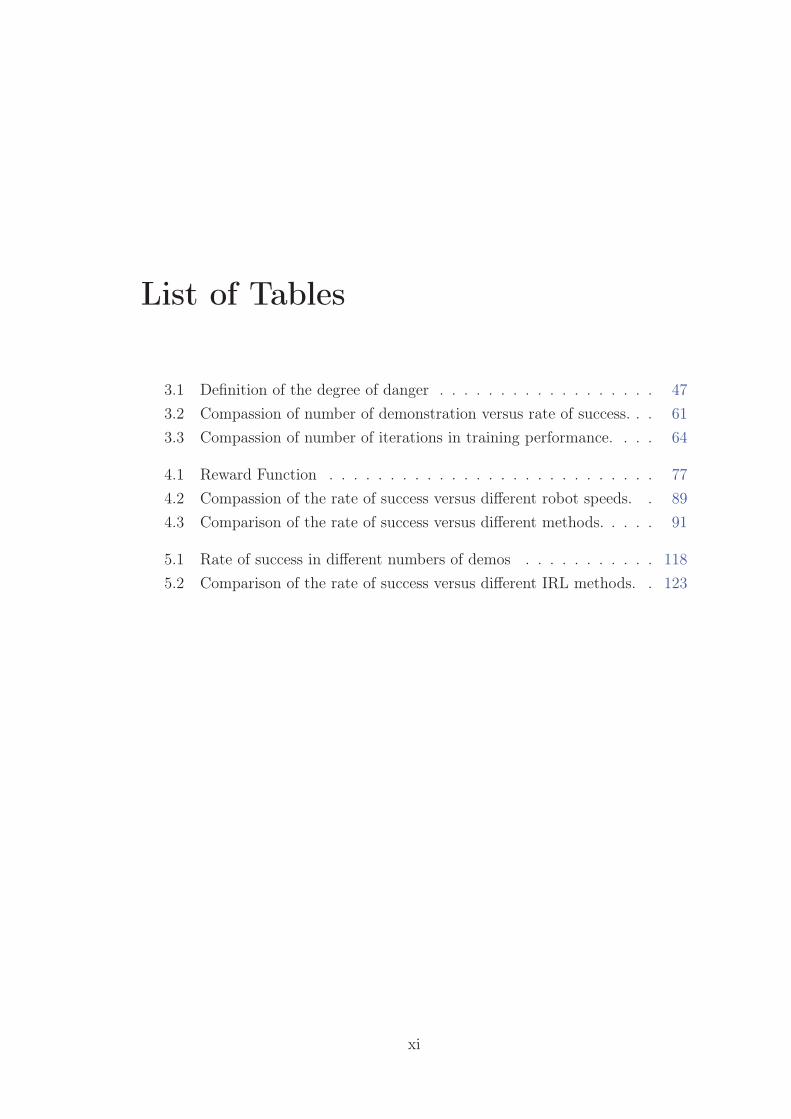
List of Tables
3.1 Definition of the degree of danger . . . . . . . . . . . . . . . . . . 473.2 Compassion of number of demonstration versus rate of success. . . 613.3 Compassion of number of iterations in training performance. . . . 64
4.1 Reward Function . . . . . . . . . . . . . . . . . . . . . . . . . . . 774.2 Compassion of the rate of success versus different robot speeds. . 894.3 Comparison of the rate of success versus different methods. . . . . 91
5.1 Rate of success in different numbers of demos . . . . . . . . . . . 1185.2 Comparison of the rate of success versus different IRL methods. . 123
xi

LIST OF TABLES
xii

List of Algorithms
1 Policy Iteration (Sutton & Barto, 1998) . . . . . . . . . . . . . . . 242 Value Iteration (Sutton & Barto, 1998) . . . . . . . . . . . . . . . 263 Policy Learning from Multiple Demonstrations . . . . . . . . . . . 534 Modified A* algorithm . . . . . . . . . . . . . . . . . . . . . . . . 555 One-step Q-learning algorithm (Watkins, 1989) . . . . . . . . . . 716 On-policy SARSA algorithm (Rummery & Niranjan, 1994) . . . . 727 SARSA with linear function approximation (Poole & Mackworth,
2010) . . . . . . . . . . . . . . . . . . . . . . . . . . . . . . . . . . 748 Training algorithm of NNQL . . . . . . . . . . . . . . . . . . . . . 829 Robot Navigation using NNQL . . . . . . . . . . . . . . . . . . . 8310 The NIRL algorithm . . . . . . . . . . . . . . . . . . . . . . . . . 111
xiii

LIST OF ALGORITHMS
xiv

Abbreviations
N - Natural numbersR - Real numbersAGV - Automated guided vehicleAMR - Autonomous mobile robotANN - Artificial neural networkAUV - Autonomous underwater vehicleBPNN - Backpropagation neural networkCNN - Convolutional neural networkDP - Dynamic programmingFFNN - Feedforward neural networkGPI - Generalized policy iterationIRL - Inverse reinforcement learningLfD - Learning from demonstrationMAP - Maximum a posterioriMC - Monte CarloMDP - Markov decision processML - Maximum likelihoodNN - Neural networkNNQL - Neural network based Q-learningPI - Policy iterationPOMDP - Partial observable Markov decision processRL - Reinforcement learningSGD - Stochastic gradient descentTD - Temperal differenceUAV - Unmanned aerial VehicleUGV - Unmanned ground vehicle
xv

ABBREVIATIONS
VI - Value iteration
xvi

Chapter 1
Introduction
Contents1.1 Background and Motivation . . . . . . . . . . . . . . . 1
1.1.1 Mobile Robotics . . . . . . . . . . . . . . . . . . . . . 1
1.1.2 Autonomous Navigation . . . . . . . . . . . . . . . . . 3
1.1.3 Robot Learning . . . . . . . . . . . . . . . . . . . . . . 5
1.1.4 Motivation . . . . . . . . . . . . . . . . . . . . . . . . 7
1.2 Contributions of the Dissertation . . . . . . . . . . . . 9
1.3 Organization of the Dissertation . . . . . . . . . . . . 10
1.1 Background and Motivation
1.1.1 Mobile Robotics
Robots are rapidly developing from industrial environments, which are physicallyfixed to their working places, to increasingly complex machines capable of per-forming challenging tasks in our daily environment. Traditional industrial robotsused in manufacturing plants∗ where the environment is highly controlled areusually more-or-less stationary.
By contrast, mobile robots are the robotic systems that can operate in un-constrained environments and have the capability to move around freely using,
∗This kind of robots are often referred to as robotic arms or manipulators.
1

1. INTRODUCTION
(a) Curiosity : NASA’s Mars explorationRover.
(b) Blackghost : an AUV designed to un-dertake an underwater assault course au-tonomously with no outside control.
(c) Kiva Robots: that Amazon used to helpemployees in their warehouses.
(d) RP-VITA: a medical robot that doctorscan make remote visits to patients via PCsor iPads running the robots.
Figure 1.1: Various applications of mobile robots.
for example, wheels. They can operate autonomously in a partially unknown andunpredictable environment without the need for physical or electro-mechanicalguidance devices (autonomous mobile robot (AMR)). Alternatively, mobile robotscan rely on guidance devices that allow them to travel a predefined navigationroute in relatively controlled space (automated guided vehicle (AGV)).
Mobile robots have been widely used in various fields, such as space explo-ration (see Figure 1.1(a)), under water survey (see Figure 1.1(b)), industrial andmilitary industries (see Figure 1.1(c)), and medical service applications (see Fig-ure 1.1(d)), and so on.
In this dissertation, we place our focus on autonomous mobile robots, robotsthat are capable of making their own decisions depending on the situation at
2

1.1 Background and Motivation
hand rather than merely executing a pre-defined sequence of motions. In fact,since most robots equipped with such decision-making capabilities are mobile,we may treat an autonomous mobile robot as a mobile robot with the ability tomake decisions.
Advances in autonomous mobile robots also have provided solutions to com-plex tasks previously only considered achievable by humans. Such domains in-clude planetary or underwater exploration (Helmick et al., 2006; Kunz et al.,2008), operation in urban environments (Bohren et al., 2008) and unmannedflight (Fabiani et al., 2007).
For a comprehensive understanding of autonomous mobile robots, readers arerecommended to see Siegwart et al. (2011); Tzafestas (2013) as references.
1.1.2 Autonomous Navigation
A fully autonomous robot can gain information about the environment, work foran extended period without human intervention, move either all or part of itselfthroughout its operating environment without human assistance, avoid situationsthat are harmful to people, property. An autonomous robot may also learn orgain new knowledge like adjusting for new methods of accomplishing its tasks oradapting to changing surroundings. Therefore, mobile robots need to have thecapabilities of autonomy and intelligence, and to design algorithms that allow therobots to function autonomously in unstructured, dynamic, partially observable,and uncertain environments pose a challenge to researchers to deal with keyissues such as uncertainty (in both sensing and action), reliability, and real-timeresponse.
In each of those domains of mobile robot applications, mobility is almostpointless without the ability to navigate. Random movement, which does notrequire a navigation capability, may be useful for certain surveillance or cleaningoperations, but for most scientific or industrial applications of mobile robots theability to move in a purposeful manner is required. Hence, autonomous navigationplays a key role in the success of the robots, and also the baseline for the relativetechnologies of autonomous mobile robots.
A mobile robot navigation task refers to plan a path with obstacle avoidanceto a specified goal and to execute this plan based on sensor readings. Mobilerobots navigation roughly includes the following six interrelated competences:
3

1. INTRODUCTION
1. Perception: to obtain and interpret sensory information;
2. Exploration: the strategy that guides the robot to select the next directionto go;
3. Mapping: to construct a spatial representation or an environment modelby using the sensory information perceived;
4. Localization: the strategy to estimate the robot position within the spatialmap that occurs simultaneously to navigation control;
5. Path planning: the strategy to find a path towards a goal location beingoptimal or not;
6. Path execution: to determine and adapt motor actions to environmentalchanges, also including obstacle avoidance.
A robot requires a mechanism that allows it to move freely in the environment,i.e., it must be able to detect and react to situations. It is the robot sensors thatplay such a role as the eyes of robots, and the robot know where it is or how it getto some place, or to be able to reason about where it has gone. The sensors can beflexible and mobile to measure the distance that wheels have traveled along theground, to measure inertial changes and external structure in the environment.Knudson & Tumer (2011) summarized that the sensors may be roughly dividedinto two classes: internal state sensors, such as accelerometers, gyroscope, whichprovide the internal information about the robot’s movements, and external statesensors, such as laser, infrared sensors, sonar, and visual sensors, which providethe external information about the environment. The data from internal statesensors may provide position estimates of the robot in a 2D space. The data fromexternal state sensors may be used to directly recognize a place or a situation,or be converted to information in a map of the environment. In most cases,the sensor readings are imprecise and unreliable due to the noises. Therefore,it is important for the mobile robot navigation to process the sensor data withnoises. Since neural networks have many processing nodes, each with primarilylocal connections, they may provide some degree of robustness or fault tolerancefor interpretation of the sensor data.
4

1.1 Background and Motivation
To sum up, the autonomous navigation task is the ability for mobile robotsto obtain enough information about the environment, process it, and act, movingsafely through this environment, usually according to a predefined path. Theability to sense the surrounding environment is a fundamental requirement toany autonomous system. All action decisions are made based on what sensoryinputs the robot perceive.
1.1.3 Robot Learning
Autonomous robots cannot always be programmed to execute predefined actionsbecause one does not always know in advance the unpredicted situations that therobot might encounter. Today, however, most robots used in the industry arepreprogrammed and require a well-defined and controlled environment. Repro-gramming such robots is often a costly process requiring an expert. By enablingrobots to learn tasks either through autonomous self-exploration or through guid-ance from a human teacher, robot installation and task reprogramming are simpli-fied. Meanwhile, robots that cannot learn lack one of the most interesting aspectsof intelligence. Recent researches has shown a drift toward artificial intelligenceapproaches to improve the robot autonomous ability based on accumulated expe-riences, and artificial intelligence methods can be computationally less expensivethan classical ones. Machine learning approaches are often applied, to each theburden on system engineers. Learning therefore has become a central topic inmodern robotics research.
Robot learning is a research field at the intersection of machine learning androbotics. It studies techniques allowing a robot to acquire novel skills or adaptto its environment through learning algorithms.∗ The embodiment of the robot,situated in a physical embedding, provides at the same time specific difficulties(e.g. high-dimensionality, real time constraints for collecting data and learning)and opportunities for guiding the learning process.
Robot learning consists of a multitude of machine learning approaches, partic-ularly reinforcement learning, imitation learning, inverse reinforcement learning,and regression methods, that have been adapted sufficiently to domain so thatthey allow learning in complex robot systems such as helicopters, flapping-wing
∗https://en.wikipedia.org/wiki/robot_learning
5

1. INTRODUCTION
flight, legged robots, anthropomorphic arms and humanoid robots. While classi-cal artificial intelligence-based robotics approaches have often attempted to man-ually generate a set of rules and models that allows the robot systems to senseand act in the real-world, robot learning centers around the idea that it is unlikelythat we can foresee all interesting real-world situations sufficiently accurate.
While robot learning covers a wide range of fields, from learning to perceive, toplan, to make decisions, etc., we focus our work on learning control in simulatedor actual physical robots. In general, learning control refers to the process of ac-quiring a particular control system and a particular task by trial and error (Schaal& Atkeson, 2010). Reinforcement learning (RL) and learning from demonstration(LfD) are mentioned as two popular families of algorithms for learning policiesfor sequential decision problems (Cobo et al., 2014).
Reinforcement learning algorithms solve sequential decision problems posed asMarkov decision processes (MDPs), learning a policy by letting the agent explorethe effects of different actions in different situations while trying to maximize asparse reward signal. RL has been successfully applied to a variety of scenarios.
Learning from demonstration is an approach to robot/agent learning thattakes as input demonstrations from a human in order to build action or taskmodels. There are a broad range of approaches that fall under the umbrella ofLfD research(Argall et al., 2009). These demonstrations are typically representedas state-action tuples, and the LfD algorithm learns a policy mapping from states(input) to actions (output) based on the examples seen in the demonstrations.Inverse reinforcement learning (IRL), as one important branch of LfD methods,addresses the problem of estimating the reward function of an agent acting in adynamic environment.
Another approach is to provide a mapping from sensory inputs to actionsthat statistically capture the key behavioral objectives without needing a modelor detailed domain knowledge (Cummins & Newman, 2007). Such methods arewell-suited to domains where the tools available to learn from past experienceand adapt to emergent conditions are limited.
With the advent of increasingly efficient robot learning methods, one can ob-serve a growing number of successful applications in robotics, such as autonomoushelicopter control (Abbeel et al., 2007, 2010; Ng et al., 2006), self-driving car(Montemerlo et al., 2008; Thrun et al., 2006; Urmson et al., 2008), autonomous
6

1.1 Background and Motivation
(a) BRETT is learning how to screw a cap ontoa water bottle.
(b) Learning to flip an artificial pancake.
Figure 1.2: Various applications of robot learning.
underwater vehicles (AUVs) control (Carreras et al., 2005), mobile robot naviga-tion (Jaradat et al., 2011), robot soccer control (Riedmiller et al., 2009).
Recently, several interesting applications have appeared. Levine et al. (2015)worked with a Willow Garage Personal Robot 2 (PR2), named Berkeley Robotfor the Elimination of Tedious Tasks (BRETT), and empowered BRETT hasacquired the ability to learn to perform various tasks on its own via trial and error,without pre-programmed details about its surroundings. Those tasks includeassembling a wheel part onto a toy airplane, stacking a Lego block, and screwinga cap on a water bottle (see Figure 1.2(a)). Mülling et al. (2013) used imitationand reinforcement learning techniques to enable a Barrett WAM arm to learnsuccessful hitting movements in table tennis. Kormushev et al. (2010) taughta robot to flip a pancake. (see Figure 1.2(b)). Other successful robot learningapplications also include Kolter & Ng (2009); Ratliff et al. (2009b).
1.1.4 Motivation
The ability of autonomous navigation plays an important role in the state-of-the-art self-driving cars. Dating back to 2003, the Defense Advanced ResearchProjects Agency (DARPA) of US government launched the “Grand Challenge” tospur the development of technologies needed to create the first fully autonomousground vehicles capable of completing a substantial off-road course within a lim-ited time. The Challenge required robotic vehicles to navigate a 142-mile longcourse through the Mojave desert in no more than 10 h. The first competition
7

1. INTRODUCTION
was held on March 13, 2004. Unfortunately, None of the 15 participating vehi-cles have ever completed more than 5% of the entire course. Therefore, a secondDARPA Grand Challenge event was scheduled on October 8, 2005. Five of 23vehicles successfully conquered the course, and Stanford’s “Stanley” (see Figure1.3) was crowned the winner with a result of 6 h 53 min (Thrun et al., 2006).This robotic car was a milestone in the quest for the modern self-driving cars.
Figure 1.3: Stanley: The 2005 DARPA Grand Challenge Winner. (Thrun et al.,2006)
Two years later, the “DARPA Urban Challenge” took place on November 3,2007, and called for autonomous vehicles to drive 97 km through a mock urbanenvironment in less than 6 hours, interacting with other moving vehicles andobstacles and obeying all traffic regulations. The vehicle “Boss” was declared thewinner (Urmson et al., 2008) and “Junior” won the second place (Montemerloet al., 2008). These vesicles were also regarded as the initial prototype of theGoogle self-driving car.
In a traditional programming scenario, a human programmer would use hu-man understanding of the desired task and have to reason in advance to codea robot controller that is capable of responding to any situation the robot mayface, no matter how unlikely. While such specialized programming is highly effi-cient, it is also expensive and limited to the situations the human operator hadconsidered. If errors or new circumstances arise after the robot is deployed, theentire costly process may need to be repeated. While the mentioned DARPA
8

1.2 Contributions of the Dissertation
challenges were competed in unrehearsed courses, it is hard to imagine that allpossible tasks can be preprogrammed. Therefore, robots need to be able to learn,either by themselves or with the help of supervision.
Motivated by the DARPA challenges and Google self-driving car, this disser-tation concentrates on ensuring that robots can learn new skills and improve theirexisting abilities autonomously, and providing robots with the ability of makingrational, intelligent decisions. By this means, robots can learn how to optimallyadapt to uncertainty and unforeseen changes in order to tackle stochastic anddynamic environments.
1.2 Contributions of the Dissertation
This dissertation considers the intelligent control in autonomous navigation viarobot learning from sensory inputs. The aim is for robot capabilities to be moreeasily extended and adapted to novel situations, even by users without program-ming ability.
We developed our research by investigating three major learning algorithms:reinforcement learning, learning from demonstration, and inverse reinforcementlearning. The main contributions of this dissertation are summarized as follows:
1. Traditional reinforcement learning has a limitation of generalization of un-visited states, which also caught many researchers’ attentions. Neural net-work, as a powerful supervised learning algorithm, can alleviate this prob-lem due to its good generalization performance. Therefore, neural networkwas incorporated into reinforcement learning, and this method largely im-proved learning ability.
2. When we recall that how humans learn new things or skills during child-hood, the word “imitation” comes to our mind. Robots should also acquirethe basic instinct of imitating. Learning from demonstration, or imitationlearning, is a good tool to enable robots to learn behaviors from expertdemonstrations. We deduced a policy learning method that efficiently pro-vided robots with a learning ability that can adapt to changing environ-ments.
9

1. INTRODUCTION
3. When experts could demonstrate optimal examples, learning from demon-strations showed sufficiently good performance. Most of the time, how-ever, non-optimal examples are also provided. In such cases, learning fromdemonstrations may lead to poor performance. A better way is to learn therewards in demonstrated states and then generalize to all undemonstratedstates. Based on inverse reinforcement learning, or apprenticeship learning,we developed a method by introducing neural network, and we achieved afast and robust learning algorithm.
All these three proposed methods were applied to mobile robot navigationexperiments. From the results, we can safely conclude that our methods succeededin endowing robots with learning abilities both by themselves via trial and errorand by human demonstrations.
1.3 Organization of the Dissertation
This dissertation is organized as follows.
• In Chapter 2, we begin by formalizing the Markov Decision Processes(MDPs) and partially observable Markov decision processes (POMDPs)frameworks. We also review some standard algorithms for solving MDPs,known as dynamic programming. Then we presents some reinforcementlearning algorithms that can be used in robotics.
• Chapter 3 begins by outlining the framework of learning from demonstration(LfD), from which we investigate its application on robotics. We presenta method for learning stochastic policies from expert demonstrations andfinding good controllers. Our method also applies well to autonomous nav-igation tasks, and uses a small amount of examples to learn from largeand complicated sensor data. In real-world applications, examples cannotoften be given by human experts, therefore, we give a modified version ofA* pathfinding algorithm to simulate expert examples, which can generatepaths much faster and is more adaptable to our problem.
10

1.3 Organization of the Dissertation
• In Chapter 4, we investigate the self-learning ability of autonomous robotswithout expert demonstrations. We present a method under the reinforce-ment learning framework and use the artificial neural network to generalizeand optimize the self-learning process. We successfully test our method inautonomous navigation tasks both in static and dynamic environments.
• In Chapter 5, we consider the potential damage to robots caused by failureduring self-learning process, and we describe inverse reinforcement learningthat robots learn rewards via interactions with the environment. We presentour method neural inverse reinforcement learning, which incorporates neuralnetwork into inverse reinforcement learning and the robot learns a rewardfunction as well as a policy.
• To conclude, Chapter 6 summaries the key points of our research and out-lines avenues for further research.
11

1. INTRODUCTION
12

Chapter 2
Markov Decision Processes andReinforcement Learning in Robotics
Contents2.1 Introduction . . . . . . . . . . . . . . . . . . . . . . . . 14
2.2 Markov Decision Processes . . . . . . . . . . . . . . . . 15
2.2.1 Policies and Value Functions . . . . . . . . . . . . . . 16
2.2.2 Partially Observable Markov Decision Processes . . . . 20
2.3 Dynamic Programming: Model-Based Algorithms . . 22
2.3.1 Policy Iteration . . . . . . . . . . . . . . . . . . . . . . 24
2.3.2 Value Iteration . . . . . . . . . . . . . . . . . . . . . . 25
2.4 Reinforcement Learning: Model-Free Algorithms . . 26
2.4.1 Goals of Reinforcement Learning . . . . . . . . . . . . 27
2.4.2 Monte Carlo Methods . . . . . . . . . . . . . . . . . . 28
2.4.3 Temporal Difference Methods . . . . . . . . . . . . . . 29
2.5 Mobile Robot Model . . . . . . . . . . . . . . . . . . . 30
2.5.1 Uncertainty in Mobile Robots . . . . . . . . . . . . . . 32
2.6 Conclusion . . . . . . . . . . . . . . . . . . . . . . . . . . 33
13

2. MARKOV DECISION PROCESSES AND REINFORCEMENTLEARNING IN ROBOTICS
2.1 Introduction
In recent years, we have seen a fast development of using machine learning tech-niques onto robot control problems. Machine learning helps an agent to learnfrom example data or past experience to solve a given problem. In supervisedlearning, the learner is provided an explicit target for every single input, thatis, the environment tells the learner what its response should be. In contrast,in reinforcement learning, only partial feedback is given to the learner aboutthe learner’s decisions. Therefore, under the framework of RL, the learner is adecision-making agent that takes actions in an environment and receives reward(or penalty) for its actions in trying to solve a problem. After a set of trial-and-error runs, it should learn the best policy, which is the sequence of actions thatmaximizes the total reward (Sutton & Barto, 1998).
������������
���� �
�� �
�������
Figure 2.1: The mechanism of interaction between a learning agent and its envi-ronment in reinforcement learning.
Reinforcement learning is typically operated in a setting of interaction, shownin Figure 2.1: the learning agent interacts with an initially unknown environment,and receives a representation of the state and an immediate reward as the feed-back. It then calculates an action, and subsequently undertakes it. This actioncauses the environment to transit into a new state. The agent receives the newrepresentation and the corresponding reward, and the whole process repeats.
The environment in RL is typically formulated as a Markov Decision Process(MDP), and the goal is to learn to a control strategy so as to maximize the totalreward which represents a long-term objective. In this chapter, we introduces the
14

2.2 Markov Decision Processes
structural background of Markov Decision Process and reinforcement learning inrobotics.
2.2 Markov Decision Processes
A Markov Decision Process describes a sequential decision-making problem inwhich an agent must choose the sequence of actions that maximizes some reward-based optimization criterion (Puterman, 1994; Sutton & Barto, 1998). Formally,an MDP is a tuple M = {S,A, T , r, γ}, where
• S = {s1, . . . , sN} is a finite set of N states that represents the dynamicenvironment,
• A = {a1, . . . , ak} is a set of k actions that could be executed by an agent,
• T : S × A × S �−→ [0, 1] is a transition probability function, or transitionmodel, where T (s, a, s′) stands for the state transition probability uponapplying action a ∈ A in state s ∈ S leading to state in state s′ ∈ S, i.e.T (s, a, s′) = P (s′ | s, a),
• r : S × A �−→ R is a reward function with absolute value bounded byRmax; r(s, a) denotes the immediate reward incurred when action a ∈ A isexecuted in state s ∈ S,
• γ ∈ [0, 1) is a discount factor.
Given an MDP M, the agent-environment interaction in Figure 2.1 happensas follows: let t ∈ N denote the current time, let St ∈ S and At ∈ A denote therandom state of the environment and the action chosen by the agent at time t,respectively. Once the action is selected, it is sent to the system, which makes atransition:
(St+1, Rt+1) ∼ P (· |St, At). (2.1)
In particular, St+1 is random and P (St+1 = s′ |St = s, At = a) = T (s, a, s′)
holds true for any s, s′ ∈ S, a ∈ A. Furthermore, E [Rt+1 |St, At] = r(St, At). Theagent then observes the next state St+1 and reward Rt+1, chooses a new actionAt+1 ∈ A and the process is repeated.
15

2. MARKOV DECISION PROCESSES AND REINFORCEMENTLEARNING IN ROBOTICS
The Markovian assumption (Sutton & Barto, 1998) implies that the sequenceof state-action pairs specifies the transition model T :
P (St+1 |St, At, · · · , S0, A0) = P (St+1 |St, At). (2.2)
State transitions can be deterministic or stochastic. In the deterministic case,taking a given action in a given state always results in the same next state; whilein the stochastic case, the next state is a random variable.
The goal of the learning agent is to figure out a theory of choosing the actionsso as to maximize the expected total discounted reward:
R =∞∑t=0
γtRt+1. (2.3)
If γ < 1 then the rewards received far in the future are exponentially lessworthy than those received at the first stage.
2.2.1 Policies and Value Functions
The agent selects its actions according to a special function called policy. Apolicy is defined as a mapping π : S × A �−→ [0, 1] that assigns to each s ∈ S adistribution π(s, ·) over A, satisfying
∑a∈A π(a | s) = 1, ∀s ∈ S.
A deterministic stationary policy is the case that for all s ∈ S, π(· | s) isconcentrated on a single action, i.e. at any time t ∈ N, At = π(St). A stochasticstationary policy is a function that maps each state into a probability distributionover the different possible actions, i.e., At ∼ π(· |St). The class of all stochasticstationary policies is denoted by Π.
Application of a policy is done in the following way. First, a start stateS0 is generated. Then, the policy π suggests the action A0 = π(S0) and thisaction is performed. Based on the transition function T and reward function r,a transition is made to state S1, with a probability T (S0, A0, S1) and a rewardR1 = r(S0, A0, S1) is received. This process continues, producing a sequenceS0, A0, R1, S1, A1, R2, S2, A2, ..., as shown in Figure 2.2.
Value functions are functions of states (or of state-action pairs) that estimatehow good it is for the agent to be in a given state (or how good it is to perform agiven action in a given state). The notion of "how good" here is defined in terms
16

2.2 Markov Decision Processes
�� �� �� ��
�� �� ��
�� �� ��
Figure 2.2: Decision network of a finite MDP.
of future rewards that can be expected, or, to be precise, in terms of expected
return. Of course the rewards the agent can expect to receive in the future depend
on what actions it will take. Accordingly, value functions are defined with respect
to particular policies (Sutton & Barto, 1998).
Given a a policy π, the value function is defined as a function V π : S �−→ R
that associates to each state the expected sum of rewards that the agent will
receive if it starts executing policy π from that state:
V π(s) = Eπ
[ ∞∑t=0
γtr(St, At) |S0 = s
], ∀s ∈ S. (2.4)
St is the random variable representing the state at time t, At is the random
variable corresponding to the action taken at that time instant and is such that
P (At = a |St = s) = π(s, a). (St, At)t≥0 is the sequence of random state-action
pairs generated by executing the policy π.
17

2. MARKOV DECISION PROCESSES AND REINFORCEMENTLEARNING IN ROBOTICS
The value function of a stationary policy can also be recursively defined as:
V π(s) = Eπ
[ ∞∑t=0
γtr(St, At) |S0 = s
]
= Eπ
[r(S0, A0) +
∞∑t=1
γtr(St, At) |S0 = s
]
= r(s, π(s)) + Eπ
[ ∞∑t=1
γtr(St, At) |S0 = s
]
= r(s, π(s)) + γEπ
[ ∞∑t=0
γtr(St, At) |S0 ∼ T (s, π(s), ·)]
= r(s, π(s)) + γ∑s′∈S
T (s, π(s), s′)V π(s′),
(2.5)
where π(s) is the action associated to state s.
If the uncertainty of a stochastic policy π(s) is taken into account, V π(s) can
also be specifically written as:
V π(s) =∑
a∈A(s)
π(s, a)
(r(s, a) + γ
∑s′∈S
T (s, a, s′)V π(s′)
). (2.6)
Similarly, the action-value function Qπ : S × A �−→ R underlying a policy π
is defined as
Qπ(s, a) = Eπ
[ ∞∑t=0
γtr(St, At) |S0 = s, A0 = a
], (2.7)
where St is distributed according to π(St, ·) for all t > 0. Finally, we defined the
advantage function associated with π as
Aπ = Qπ(s, a)− V π(s). (2.8)
A policy that maximizes the expected total discounted reward over all states
is called an optimal policy, denoted π∗. For any finite MDP, there is at least one
optimal policy.
The optimal value function V ∗ and the optimal action-value function Q∗ are
18
2.2 Markov Decision Processes
defined by
V ∗(s) = supπ
V π(s), s ∈ S,
Q∗(s, a) = supπ
Qπ(s, a), s ∈ S, a ∈ A.(2.9)
Moreover, the optimal value- and action-value functions are connected by thefollowing equations:
V ∗(s) = supa∈A
Q∗(s, a), s ∈ S, (2.10)
Q∗(s, a) = r(s, a) + γ∑s′∈S
P (s′ | s, a)V ∗(s′), s ∈ S, a ∈ A. (2.11)
It turns out that V ∗ and Q∗ satisfy the so-called Bellman optimality equations(Puterman, 1994). In particular,
Q∗(s, a) = r(s, a) + γ∑s′∈S
P (s′ | s, a)maxb∈A
Q∗(s′, b), (2.12)
V ∗(s) = maxa∈A
r(s, a) + V ∗(s′). (2.13)
We call a policy that satisfies∑
a∈A π(a | s)Q(s, a) = maxa∈A Q(s, a) at allstates s ∈ S greedy w.r.t. the function Q. It is known that all policies that aregreedy w.r.t. Q∗ are optimal and all stationary optimal policies can be obtainedthese way.
Here, we present the following important results concerning MDP (Sutton &Barto, 1998):
Theorem 2.1 (Bellman Equations). Let a Markov Decision Problem M =
{S,A, T , r, γ} and a policy π : S × A −→ [0, 1] be given. Then, ∀s ∈ S, a ∈ A,V π and Qπ satisfy
V π(s) = r(s, π(s)) + γ∑s′∈S
T (s, π(s), s′)V π(s′), (2.14)
Qπ(s, a) = r(s, a) + γ∑s′∈S
T (s, a, s′)V π(s′). (2.15)
Theorem 2.2 (Bellman Optimality). Let a Markov Decision Problem M =
{S,A, T , r, γ} and a policy π : S × A −→ [0, 1] be given. Then, π is an optimal
19

2. MARKOV DECISION PROCESSES AND REINFORCEMENTLEARNING IN ROBOTICS
policy for M if and only if, ∀s ∈ S,
π(s) ∈ argmaxa∈A
Qπ(s, a). (2.16)
The transition probability T (s, a, s′) = P (s′ | s, a).
2.2.2 Partially Observable Markov Decision Processes
In the setting of an MDP, the agent should obtain a precise state informationof the environment at any moment. Unfortunately, this assumption may nothold in practice in respect that the agent observes the world through limitedand imperfect receptors, and the information contained in the perceptions isnot sufficient for determining the state. Partially Observable Markov DecisionProcesses (POMDPs) (Smallwood & Sondik, 1973) was introduced to handlesuch cases.
Formally, a POMDP is a tuple 〈S,A, T ,O, Z, R〉 where 〈S,A, T , R〉 is anMDP, and:
• O is a set of observations (perceptions),
• Z is an observation function: Z(o, s, a) is the probability of observing o ∈ Oif the state of the system is s and the action that led to this state is a.
The observations can be aliased (the same observation may be observed indifferent states) and stochastic (different observations may be observed in thesame state). Consequently, the state of the system cannot be determined fromthe observations. Instead, an observation can be seen as an evidence about thestate. The agent’s belief about the hidden state is a probability distribution onall the possible states, called the belief state:
bt =[Pr(st = x0), P r(st = x1), . . . , P r(st = s|S|−1)
]�(2.17)
The agent starts with an initial belief state b0, and every time an action at
is executed and an observation ot+1 is received, the belief state bt is updated byusing Bayes’ Rule:
20

2.2 Markov Decision Processes
bt+1(x) = Pr(st+1 = s | bt, at, ot+1)
=Pr(st+1 = s, ot+1 | bt, at)
Pr(ot+1 | bt, at)
=
∑s′∈S bt(s
′)T (s, at, s′)Z(ot+1, s, at)∑
s′∈S∑
s′′∈S bt(s′)T (s′, at, s′′)Z(ot+1, s′′, at)
(2.18)
Therefore, the belief state bt+1 is a nonlinear function of the previous beliefstate bt, action at and observation ot+1:
bt+1 = τ(bt, at, ot+1) (2.19)
The belief state bt at time instant t allows us to calculate the probability ofany observation o at time instant t+ 1 as:
Pr(ot+1 = o | bt, at) =∑s∈S
∑s′∈S
bt(s)T (s, at, s′)Z(o, s′, at) (2.20)
The expected reward of executing action a for a belief state bt is given by:
r(a | bt) =∑s∈S
bt(s)R(s, a) (2.21)
�� �� �� ��
� � � �
��� ������ �
� �� ������ �
�� �� �� ���������
�� �� ������ ��������
� ����� �� �� ��
Figure 2.3: Schema of a Partially Observable Markov Decision Process.
21

2. MARKOV DECISION PROCESSES AND REINFORCEMENTLEARNING IN ROBOTICS
A Markovian belief state allows a POMDP to be formulated as a Markov de-cision process where every belief is a state. The resulting Belief Markov DecisionProcess will thus be defined on a continuous state space, since there are infinitebeliefs for any given POMDP (Kaelbling et al., 1998). The belief MDP is definedas a tuple 〈B,A, τ, r, γ〉 where:
• B is the set of belief states over the POMDP states,
• A is the same set of actions as for the original POMDP,
• τ is the belief state transition function,
• r : B ×A −→ R is the reward function on belief states,
• γ is the discount factor equal to the γ in the original POMDP.
In belief MDP, τ and r need to be derived from the original POMDP. For allb, b′ ∈ B, a ∈ A:
τ(b, a, b′) =∑o∈O
Pr(b′ | b, a, o)Pr(o | a, b), (2.22)
r(b, a) =∑x∈S
b(s)R(s, a). (2.23)
Figure 2.3 illustrates the temporal series of belief states. The Markov propertyimplies that the belief state and the full history of the system (sequence of actionsand observations) contain exactly the same information about the current state,and consequently, about all the future events.
2.3 Dynamic Programming: Model-Based Algo-rithms
Dynamic programming (DP) is a method for computing an optimal policy π∗ inorder to solve a given Markov decision process.
Dynamic programming assumes full knowledge of the Markov decision pro-cess, including the transition dynamics of the environment and the reward func-tion (Bertsekas, 1996). Therefore, they are classified into model-based learning
22

2.3 Dynamic Programming: Model-Based Algorithms
����
�� �
(a) Interaction of policyevaluation and improve-ment processes
�
����
����
(b) The convergence of both the value function and the pol-icy to their optimals
Figure 2.4: Generalized Policy Iteration (Sutton & Barto, 1998)
algorithms. On the contrary are model-free learning algorithms, which do not
require a perfect model of the environment, and will be introduced them later in
this chapter.
Dynamic programming algorithms for solving MDPs can be categorized into
one of the two families: value iteration (VI) and policy iteration (PI) (Sutton &
Barto, 1998). Both of these approaches share a common underlying mechanism,
the generalized policy iteration (GPI) principle (Sutton & Barto, 1998), depicted
in Figure 2.4. This principle consists of two interaction processes. The first step,
policy evaluation, estimates the utility of the current policy π, that is, it computes
the value V π. This step gathers information about the policy for computing
the second step, the policy improvement step. In this step, the values of the
actions are evaluated for every state, in order ot find possible improvements,
that is, possibly other actions in particular states that are better than the action
the current policy proposes. This step computes an improved policy π′ from
the current policy π using the information in V π. As long as both processes
continue to update all states, the ultimate goal is to converge to the optimal value
function and an optimal policy. Figure 2.4(b) presents a geometric metaphor for
convergence of both the value function and the policy in GPI.
23

2. MARKOV DECISION PROCESSES AND REINFORCEMENTLEARNING IN ROBOTICS
2.3.1 Policy Iteration
Policy iteration iterates between the two processes of GPI. This is repeated untilconverging to an optimal policy. This method is depicted in Algorithm 1.
Algorithm 1 Policy Iteration (Sutton & Barto, 1998)Input: An MDP model 〈S,A, T , r, γ〉;/* Initialization */
1: t = 0, k = 0;2: ∀s ∈ S: Initialize πt(s) with an arbitrary action;3: ∀s ∈ S: Initialize Vk(s) with an arbitrary value;4: repeat
/* Policy evaluation */5: repeat6: ∀s ∈ S : Vk+1(s) = r(s, πt(s)) + γ
∑s′∈S T (s, πt(s), s
′)Vk(s′);
7: k ← k + 1;8: until ∀s ∈ S : |Vk(s)− Vk−1(s)| < ε;
/* Policy improvement */9: ∀s ∈ S : πt+1(s) = argmaxa∈A
[r(s, a) + γ
∑s′∈S T (s, a, s′)Vk(s
′)];
10: t ← t+ 1;11: until πt = πt−1;12: π∗ = πt;
Output: An optimal policy π∗.
It consists in starting with a randomly chosen policy πt and a random ini-tialization of the corresponding value function Vk, for k = 0 and t = 0 (Steps 1to 3), and iteratively repeating the policy evaluation and the policy improvementoperations.
Policy evaluation (Steps 5 to 8) consists in calculating the action value ofpolicy πt+1 by solving the solving the equation (2.15) for all the states s ∈ S.An efficient iterative way to solve this equation is to initialize the value functionof πt+1 with the value function Vk of the previous policy, and then repeat theoperation:
∀s ∈ S : Vk+1(s) = r(s, πt(s)) + γ∑s′∈S
T (s, πt(s), s′)Vk(s
′), (2.24)
until ∀s ∈ S : |Vk(s)− Vk−1(s)| < ε, for a predefined error threshold ε.
Policy improvement (Steps 9 to 10) consists in finding the greedy policy πt+1
24

2.3 Dynamic Programming: Model-Based Algorithms
given the value function Vk:
∀s ∈ S : πt+1(s) = argmaxa∈A
[r(s, a) + γ
∑s′∈S
T (s, a, s′)Vk(s′)
]. (2.25)
This process stops when πt = πt−1, in which case πt is an optimal policy, i.e.,π∗ = πt.
In sum, PI generates a direct sequence of alternating policies and value func-tions:
π0 → V π0 → π1 → V π1 → · · · → π∗ → V ∗ → π∗
The policy evaluation processes occur in the transitions of πt → V πt ; whilethe V πt → πt+1 conversions are realized by the policy improvement processes.
2.3.2 Value Iteration
The main drawback of policy iteration is that a complete policy evaluation isinvolved in each iteration. Value iteration consists in overlapping the evaluationand improvement processes.
Instead of completely separating the evaluation and improvement processes,the value iteration approach breaks off evaluation after just one iteration. In fact,it immediately blends the policy improvement step into its iterations, therebypurely focusing on estimating directly the value function.
Value iteration, described in Algorithm 2, can be written as a simple backupoperation:
∀s ∈ S : Vk+1(s) = maxa∈A
[r(s, a) + γ
∑s′∈S
T (s, a, s′)Vk(s′)
]. (2.26)
This operation is repeated (Steps 3 to 6) until ∀s ∈ S : |Vk(s)− Vk−1(s)| < ε,in which case the optimal policy is simply the greedy policy with respect to thevalue function Vk (Step 7).
VI produces the following sequence of value functions:
V0 → V1 → V2 → V3 → V4 → V5 → · · · → π∗
25

2. MARKOV DECISION PROCESSES AND REINFORCEMENTLEARNING IN ROBOTICS
Algorithm 2 Value Iteration (Sutton & Barto, 1998)Input: An MDP model 〈S,A, T , r, γ〉;
1: k = 0;2: ∀s ∈ S: Initialize Vk(s) with an arbitrary value;3: repeat4: ∀s ∈ S : Vk+1(s) = maxa∈A
[r(s, a) + γ
∑s′∈S T (s, a, s′)Vk(s
′)];
5: k ← k + 1;6: until ∀s ∈ S : |Vk(s)− Vk−1(s)| < ε;7: ∀s ∈ S : π∗(s) = argmaxa∈A
[r(s, a) + γ
∑s′∈S T (s, a, s′)Vk(s
′)];
Output: An optimal policy π∗.
2.4 Reinforcement Learning: Model-Free Algorithms
Reinforcement learning (RL) is a machine learning framework for solving sequen-tial decision problems that can be modeled as MDPs (Kaelbling et al., 1996).Unlike dynamic programming that assumes the availability of a perfect modelof the environment, RL is primarily concerned with how to obtain an optimalpolicy when such a model is not available. Therefore, reinforcement learning ismodel-free. In addition, RL adds to MDPs a focus on approximation and incom-plete information, and the need for sampling and exploration to gather statisticalknowledge about this unknown model.
In a RL problem, the agent and its environment may be modeled being ina state s ∈ S and can perform actions a ∈ A, each of which may be membersof either discrete or continuous sets and can be multi-dimensional. A state s
contains all relevant information about the current situation to predict futurestates. An action a is used to control the state of the system. For every step,the agent also gets a reward R, which is a scalar value and assumed to be afunction of the state and observation. It may equally be modeled as a randomvariable that depends on only these variables. In the navigation task, a possiblereward could be designed based on the energy costs for taken actions and rewardsfor reaching targets. Reinforcement learning is designed to find a policy π fromstates to actions, that picks action a in given state s maximizing the cumulativeexpected reward. The policy π is either deterministic or stochastic. The formeralways uses the exact same action for a given state in the form a = π(s), thelater draws a sample from a distribution over actions when it encounters a state,i.e., a ∼ π(s, a) = P (a|s). The reinforcement learning agent needs to discover
26

2.4 Reinforcement Learning: Model-Free Algorithms
the relations between states, actions, and rewards. Hence exploration is requiredwhich can either be directly embedded in the policy or performed separatelyand only as part of the learning process. Different types of reward functions arecommonly used, including rewards depending only on the current state R = R(s),rewards depending on the current state and action R = R(s, a), and rewardsincluding the transitions R = R(s′, a, s).
A detailed survey of reinforcement learning in robotics can be found in (Koberet al., 2013).
2.4.1 Goals of Reinforcement Learning
The goal of reinforcement learning is to discover an optimal policy π∗ that mapsstates or observations to actions so as to maximize the expected return J , whichcorresponds to the cumulative expected reward. A finite-horizon model onlyattempts to maximize the expected reward for the horizon H, i.e., the next H
(time-)steps h:
J = E
{H∑
h=0
Rh
}. (2.27)
This setting can also be applied to model problems where it is known howmany steps are remaining.
Alternatively, future rewards can be discounted by a discount factor γ (with0 ≤ γ < 1):
J = E
{ ∞∑h=0
γhRh
}. (2.28)
Two natural goals arise for the learner. In the first, we attempt to find anoptimal strategy at the end of a phase of training or interaction. In the second,the goal is to maximize the reward over the whole time the robot is interactingwith the world.
In contrast to supervised learning, the learner must first discover its environ-ment and is not told the optimal action it needs to take. To gain informationabout the rewards and the behavior of the system, the agent needs to exploreby considering previously unused actions or actions it is uncertain about. Itneeds to decide whether to play it safe and stick to well known actions with
27

2. MARKOV DECISION PROCESSES AND REINFORCEMENTLEARNING IN ROBOTICS
(moderately) high rewards or to dare trying new things in order to discover newstrategies with an even higher reward. This problem is commonly known as theexploration-exploitation trade-off.
RL relies on the interaction between a learning agent and its environment (seeFigure 2.1), the process is similar:
1. A learning agent interacts with its environment in discrete time steps;
2. At each time step t, the agent observes the environment, and receives arepresentation of state st and a reward rt;
3. The agent infers an action at, and subsequently undertaken in the environ-ment.
4. The agent observes the new environment, and receives a new state repre-sentation st+1 and an associated reward rt+1.
Based on how the agent chooses an action, RL can be distinguished betweenoff-policy and on-policy methods. Off-policy algorithms learn independent of theemployed policy, i.e., an explorative strategy that is different from the desired finalpolicy can be employed during the learning process. On-policy algorithms collectsample information about the environment using the current policy. As a result,exploration must be built into the policy and determines the speed of the policyimprovements. Such exploration and the performance of the policy can result inan exploration-exploitation trade-off between long- and short-term improvementof the policy. A simple exploration scheme known as ε-greedy, performs a randomaction with probability ε and otherwise greedily follows the state-action values.
2.4.2 Monte Carlo Methods
Monte Carlo methods use sampling in order to estimate the value function anddiscover the optimal policy (Sutton & Barto, 1998). This procedure can be usedto replace the policy evaluation step of the dynamic programming-base methodsabove. Unlike DP, Monte Carlo methods do not assume complete knowledge ofthe environment. Monte Carlo methods are model-free, i.e., they do not needan explicit transition function. They require only experience – sample sequences
28

2.4 Reinforcement Learning: Model-Free Algorithms
of states, actions, and rewards from online or simulated interaction with an en-vironment. Learning from online experience requires no prior knowledge of theenvironment’s dynamics, yet can still attain optimal behavior. Learning fromsimulated experience requires a model, but the model need only generate sampletransitions, not the complete probability distributions of all possible transitionsthat is required by dynamic programming methods.
Monte Carlo methods solve reinforcement learning problems based on averag-ing sample returns. They perform rollouts by executing the current policy on thesystem, hence operating on-policy. The frequencies of transitions and rewardsare kept track of and used to form estimates of the value function. For exam-ple, in an episodic setting the state-action value of a given state action pair canbe estimated by averaging all the returns that were received when starting fromthem.
2.4.3 Temporal Difference Methods
Temporal Difference (TD) Methods is a combination of Monte Carlo methodsand dynamic programming methods (Sutton & Barto, 1998). Unlike Monte Carlomethods, TD learning methods do not have to wait until an estimate of the returnis available (i.e., at the end of an episode) to update the value function. Instead,they use temporal errors and only have to wait until the next time step. Thetemporal error is the difference between the old estimate and a new estimate ofthe value function, taking into account the reward received in the current sample.These updates are done iteratively and, in contrast to dynamic programmingmethods, only take into account the sampled successor states rather than thecomplete distributions over successor states. Like the Monte Carlo methods, thesemethods are model-free, as they do not use a model of the transition function todetermine the value function, and can learn directly from raw experience withouta model of the environment’s dynamics. In this setting, the value function cannotbe calculated analytically but has to be estimated from sampled transitions inthe MDP.
Q-Learning (Watkins, 1989) is a representative off-policy, model-free RL al-gorithm. It incrementally processes the transition samples. Q-value is updatediteratively by
29

2. MARKOV DECISION PROCESSES AND REINFORCEMENTLEARNING IN ROBOTICS
Q′(s, a) ← Q(s, a) + α
(r(s, a) + γmax
b∈AQ(s′, b)−Q(s, a)
). (2.29)
SARSA (Rummery & Niranjan, 1994) is a representative on-policy, model-freeRL algorithm. Different from Q-learning that uses maxb∈A Q(s′, b) for estimatingfuture rewards, SARSA uses Q(s′, a′) for a′ the action executed in s′ under thecurrent policy that generates the transition sample (s, a, , r, s′, a′). Mathemati-cally, the update rule is:
Q′(s, a) ← Q(s, a) + α (r(s, a) + γQ(s′, a′)−Q(s, a)) . (2.30)
If each action is executed in each state an infinite number of times, and forall state-action pairs (s, a), the learning rate α is decayed appropriately, theQ-values will converge with probability 1 to the optimal Q∗ (Watkins & Dayan,1992). Similar guarantee of convergence for SARSA can be found in (Singh et al.,2000) with a more strict requirement on the exploration of all states and actions.
More contents about reinforcement learning will be subsequently presented inChapter 4.
2.5 Mobile Robot Model
Figure 2.5: Robotino®: a mobile robot system for education and research.
30

2.5 Mobile Robot Model
The mobile robot model used in this dissertation is built according to themobile robot system Robotino® from Festo Didactic∗, as shown in Figure 2.5. Itis based on an omnidirectional drive assembly, which enables the system to roamfreely. The Robotino® is equipped with a total of nine infrared sensors arrangedaround its base at an angle of 40◦ to each other, and each distance sensor readsout a voltage level whose value depends on the distance to a reflective object.
Therefore, our mobile robot model is assumed to have three wheels, one infront and two in back. The robot is equipped with nine distance sensors to deter-mine the distances of objects within its surroundings. The sensors are arrangedat an angle of 40◦ to each other, and each sensor can cover a scope of detectionof 40◦, as shown in Figure 2.6. (Si){1≤i≤9} are the nine sensors and (Ri){1≤i≤9}representing the corresponding scopes of detection.
�����
��
��
��
�
�
��
���
���
����������������������
��������
���� �����������
��������
���������
���������� ��� ���
�����������
Figure 2.6: The mobile robot model with nine sensors and their correspondingsensing areas.
The robot navigation environment consists of its target and the obstacles, asshown in Figure 2.7. The initial and target positions are predefined to the robot,and the robot will try to reach the target in a collision-free path in spite of thepresence of static or moving obstacles.
dr−t is the distance between the robot and the target, and dr−o is the distancebetween the robot and the obstacle.
∗http://www.festo-didactic.com/int-en/services/robotino/
31

2. MARKOV DECISION PROCESSES AND REINFORCEMENTLEARNING IN ROBOTICS
�
�����
������
����� !�
��� �
��� �����
����
�
Figure 2.7: The mobile robot environment with a target and an obstacle.
2.5.1 Uncertainty in Mobile Robots
For mobile robots, uncertainty is everywhere. Wheels may slip, sensors may beaffected by noise, and obstacles move unpredictably. Truly autonomous robots ordecision-making agents must act in ways that are robust to these sorts of failuresand unexpected events which we may think of in general as uncertainty.
Uncertainty can take many forms, but for brevity and clarity we place ourattention to two important types (O’kane et al., 2005):
• Prediction uncertainty occurs when the effects of actions are not fullypredictable. This can be thought of as an uncertainty in future states.
• Sensing uncertainty is the uncertainty in the current state. This occurs,for example, in robots that have limited or imperfect sensing. We also admitthe case where robots have no sensing at all.
The uncertainty in mobile robots may result in the fact that when a mobilerobot tries to execute an action in a given state of environment, the action doesnot always lead to the expected result, because the information represented bythe state may not precisely determine the outcome of the actions.
32

2.6 Conclusion
2.6 Conclusion
This chapter has presented the Markov decision processes, which are the under-lying structure of robot learning methods presented in this dissertation. Severalclassical algorithms for solving MDPs were also briefly introduced. The funda-mental concepts of the reinforcement learning was then brought. Finally, wedescribe the mobile robot model that is used throughout this dissertation.
33

2. MARKOV DECISION PROCESSES AND REINFORCEMENTLEARNING IN ROBOTICS
34

Chapter 3
Policy Learning from MultipleDemonstrations
Contents3.1 Introduction . . . . . . . . . . . . . . . . . . . . . . . . 36
3.2 Related Work . . . . . . . . . . . . . . . . . . . . . . . . 37
3.3 Neural Network Model . . . . . . . . . . . . . . . . . . 38
3.3.1 Backpropagation Algorithm . . . . . . . . . . . . . . . 41
3.4 Policy Learning from Demonstrations . . . . . . . . . 45
3.4.1 Dataset Extraction from Demonstrations . . . . . . . . 46
3.4.2 Architecture of Neural Network . . . . . . . . . . . . . 48
3.4.3 Policy Learning Process . . . . . . . . . . . . . . . . . 49
3.4.4 Algorithm . . . . . . . . . . . . . . . . . . . . . . . . . 52
3.5 Demonstration by Modified A* Algorithm . . . . . . 52
3.5.1 Node Representation . . . . . . . . . . . . . . . . . . . 53
3.5.2 Algorithm . . . . . . . . . . . . . . . . . . . . . . . . . 54
3.5.3 Result . . . . . . . . . . . . . . . . . . . . . . . . . . . 54
3.6 Experimental Results . . . . . . . . . . . . . . . . . . . 56
3.6.1 Policy Learning Process . . . . . . . . . . . . . . . . . 57
3.6.2 Robot navigation in unknown environments . . . . . . 59
3.6.3 Paths Comparison . . . . . . . . . . . . . . . . . . . . 61
35

3. POLICY LEARNING FROM MULTIPLE DEMONSTRATIONS
3.6.4 Autonomous Navigation in Dynamic Environments . . 61
3.6.5 Discussions . . . . . . . . . . . . . . . . . . . . . . . . 61
3.7 Conclusion . . . . . . . . . . . . . . . . . . . . . . . . . . 64
3.1 Introduction
Nowadays, robots are designed to perform complicated tasks, such as grasping andmanipulating objects, navigating in outdoor environments, and driving in urbanroads. Traditionally, robots had to be tediously hand programmed for every taskthey performed, which is a laborious and time-intensive engineering process (Tianet al., 2015). Rather than manually pre-programming each desired behavior,an appropriate robot controller is always preferable that can be derived fromobservations of a human’s own performance. In this context, learning mechanismsare needed to acquire knowledge from such an interaction process.
Learning from demonstration (LfD) is a machine learning mechanism thatenables robotic systems to autonomously perform new tasks, and LfD is inspiredby the way humans learn from being guided by experts, from infancy throughadulthood. The main principle of robot learning from demonstration is that end-users can teach robots new tasks without programming (Billard & Grollman,2013).
The basic idea is that the robot learns a behavior from one or several demon-strations performed by a teacher. Within LfD, a mapping between world statesand actions is learned from examples, or demonstrations. One demonstration isdefined as a sequence of state-action pairs that are recorded during the teacher’sdemonstration of the desired robot behavior. LfD algorithms utilize this datasetof examples to drive a policy that reproduces the demonstrated behavior. How-ever, we also need the system to adapt to new and unseen conditions. Therefore,besides learning, generalizing is another key point to LfD, especially to tackle thecurse of dimensionality in high dimensional spaces.
We proposed our method of policy learning from multiple demonstrations (Xiaet al., 2015) by incorporating artificial neural network (ANN) into learning fromdemonstration due to its properties such as nonlinear mapping, ability to learnfrom examples, good generalization performance, and capability to approximate
36

3.2 Related Work
an arbitrary function given sufficient number of neurons. Different from directimitation learning which could only reproduce what is seen in the demonstrations,our method can hence generalize to undemonstrated states and endow robots withthe ability to learn what it means to perform a task by generalizing from observingmultiple demonstrations.
As we mentioned before, the navigating capability is quite important for mo-bile robots. However, in some hazardous cases, providing reliable demonstrationsplaces a burden on the human expert, even impossible. An alternative way is toprovide robots with computer-based examples and let robots observe and learn.Based on this assumption, we also proposed an modified version of A* pathfindingalgorithm to play the part of expert demonstrations.
3.2 Related Work
Learning from demonstration (Argall et al., 2009) can be a powerful and naturaltool for developing robot control policies. Many techniques rely upon an unknownmapping from teacher observations and actions to robot observations and actions(Alissandrakis et al., 2002; Robins et al., 2004; Ude et al., 2004). A wide variety ofdemonstration training methods have been explored in previous work, includingteleoperation (Saunders et al., 2006; van Lent & Laird, 2001), direct manipulationof the learning agent (Atkeson & Schaal, 1997), object grasping (Sweeney &Grupen, 2007), the grocery checkout task (Jain et al., 2013), etc. In Abbeel et al.(2010), acrobatic trajectories of an helicopter are learned by recording the tiltand pan motion of the helicopter when teleoperated by an expert pilot.
Nicolescu & Matarić (2001, 2003) present a learning framework based ondemonstration, generalization and teacher feedback, in which training is per-formed by having the robot follow a human and observe its actions. A high-leveltask representation is then constructed by analyzing the experience with respectto the robot’s underlying capabilities. The authors also describe a generalizationof the framework that allows the robot to interactively request help from a hu-man in order to resolve problems and unexpected situations. This interaction isimplicit as the agent has no direct method of communication; instead, it attemptsto convey its intentions by communicating though its actions.
37

3. POLICY LEARNING FROM MULTIPLE DEMONSTRATIONS
Lockerd & Breazeal (2004) and Breazeal et al. (2004) demonstrate a roboticsystem where high-level tasks are taught through social interaction. In this frame-work, the teacher interacts with the agent through speech and visual inputs, andthe learning agent expresses its internal state through emotive cues such as facialand body expressions to help guide the teaching process. The outcome of thelearning is a goal-oriented hierarchical task model. In later work (Thomaz &Breazeal, 2008), the authors examine ways in which people give feedback whenengaged in an interactive teaching task. Although the study’s focus is to examinethe use of a human-controlled reward signal in reinforcement learning, the authorsalso find that users express a desire to guide or control the agent while teach-ing. This result supports our belief that, for many robotic domains, teleoperationprovides an easy and intuitive human-robot communication method.
Bentivegna et al. (2004a,b) and Saunders et al. (2006) present demonstrationlearning approaches based on supervised learning methods. Both groups use thek-nearest neighbor (KNN) (Mitchell, 1997) algorithm to classify instances basedon similarity to training examples, resulting in a policy mapping from sensoryobservations to actions.
Chernova & Veloso (2007) represent the policy as a set of Gaussian mixturemodels, where each model, with multiple Gaussian components, corresponds toa single action.
Statistical supervised learning techniques that rely on labeled training dataare frequently used in demonstration-based learning to learn a policy given a fixedset of labeled data (Bentivegna et al., 2004a; Saunders et al., 2006).
In our work we focus on a policy learning approach, in which the robot ex-periences the demonstration through its sensors while under the control of anexpert. The task is executed by a computer-based teacher, and the details ofthe execution, in the form of paired observations and actions, are passed on tothe robot. The robot then generalizes from these demonstrations in order toeffectively execute the task itself.
3.3 Neural Network Model
An artificial neural network (ANN) (Ng, 2011; Rojas, 1996) is organized in layersand each layer is composed of a bunch of “neuron” nodes. A neuron is a compu-
38

3.3 Neural Network Model
tational unit that can reads inputs, processes them and generates an output, seeFigure 3.1 as an example.
��
��
��
��
��
�����
�����
�����
�����
�� �� �� ��� �� ���
�������
Figure 3.1: A neural network example.
The whole network is constructed by interconnecting many neurons. In thisfigure, one circle represents one neuron. The leftmost layer of the network iscalled the input layer, and the rightmost layer the output layer. The middle layerof nodes is called the hidden layer, since its values are not observed in the trainingset. The input and output layers serve respectively as the inputs and outputs ofthe neural network. The neurons labeled “+1” are called bias units. A bias unithas no input and always outputs +1. Hence, this neural network has 3 inputunits (excluding the bias unit), 3 hidden units (excluding the bias unit), and 1output unit.
We use nl to denote the number of layers and label each layer l as Ll. In Figure3.1, nl = 3, layer L1 is the input layer, and Lnl
is the output layer. The linksconnecting two neurons are named weights, representing the connection strengthbetween the neurons. The parameters inside the neural network are (W, b) =
(W (1), b(1),W (2), b(2)), where we write W(l)ij to denote the weight associated with
the connection between unit j in layer l, and unit i in layer l + 1. Also, b(l)i isthe bias associated with unit i in layer l + 1. Thus, we have W (1) ∈ R
3×3 andW (2) ∈ R
1×3.∗
∗b(l)i can also be interpreted as the connecting weight between the bias unit in layer l who
always outputs +1 and the neuron unit i in layer l+1. Thus, b(l)i may be replaced by W(l)i0 . In
39

3. POLICY LEARNING FROM MULTIPLE DEMONSTRATIONS
Each neuron in the network contains an activation function in order to controlits output. We denote the activation of unit i in layer l by a
(l)i . For the input
layer L1, a(1)i = xi, the i-th input of the whole network. For the other layers,
a(l)i = f(z
(l)i ). Here, z(l)i denote the total weighted sum of inputs to unit i in layer
l, including the bias term (e.g., z(2)i =∑n
j=1 W(1)ij xj + b
(1)i ), so that a
(l)i = f(z
(l)i ).
Given a fixed setting of the parameters (W, b), the neural network outputs areal number that is defined as the hypothesis hW,b(x). Specifically, the computa-tion that this neural network represents is given by:
a(2)1 = f(W
(1)11 x1 +W
(1)12 x2 +W
(1)13 x3 + b
(1)1 ),
a(2)2 = f(W
(1)21 x1 +W
(1)22 x2 +W
(1)23 x3 + b
(1)2 ),
a(2)3 = f(W
(1)31 x1 +W
(1)32 x2 +W
(1)33 x3 + b
(1)3 ),
hW,b(x) = a(3)1 = f(W
(2)11 a
(2)1 +W
(2)12 a
(2)2 +W
(2)13 a
(2)3 + b
(2)1 ).
(3.1)
For a more compact expression, we can extend the activation function f(·) toapply to vectors in an element-wise fashion, i.e., f([z1, z2, z3]) = [f(z1), f(z2), f(z3)],then we can write the equations above as:
a(1) = x,
z(2) = W (1)a(1) + b(1),
a(2) = f(z(2)),
z(3) = W (2)a(2) + b(2),
hW,b(x) = a(3) = f(z(3)).
(3.2)
x = [x1, x2, x3]� is a vector of values from the input layer. This computational
process, from inputs to outputs, is called forward propagation. More generally,given any layer l’s activation a(l), we can compute the activation a(l+1) of the nextlayer l + 1 as:
z(l+1) = W (l)a(l) + b(l),
a(l+1) = f(z(l+1)).(3.3)
this way, W (1) ∈ R3×4 and W (2) ∈ R
1×4.
40

3.3 Neural Network Model
In this dissertation, we will choose f(·) to be the sigmoid function f : R �→]− 1,+1[ :
f(z) =1
1 + exp(−z). (3.4)
Its derivative is given by
f ′(z) = f(z)(1− f(z)). (3.5)
The advantage of putting all variables and parameters into matrices is thatwe can greatly speed up the calculation speed by using matrix-vector operations.
Neural networks can also have multiple hidden layers or multiple output units.Taking Figure 3.2 as an example, this network has two hidden layers L2 and L3
and two output units in layer L4.
��
��
��
��
��
�� ��� �� ��� �� ���
�������
��
�� ���
Figure 3.2: A neural network example with two hidden layers.
The forward propagation applies to all architectures of feedforward neuralnetworks, i.e., to compute the output of the network, we can start with the inputlayer L1, and successively compute all the activations in layer L2, then layer L3,and so on, up to the output layer Lnl
.
3.3.1 Backpropagation Algorithm
Suppose we have a fixed training set {(x(1), y(1)), . . . , (x(m), y(m))} of m trainingexamples. We can train our neural network using batch gradient descent. Indetail, for a single training example (x, y), we define the cost function with respectto that single example to be:
41

3. POLICY LEARNING FROM MULTIPLE DEMONSTRATIONS
J(W, b; x, y) =1
2‖hW,b(x)− y‖2. (3.6)
This is a squared-error cost function. Given a training set of m examples, wethen define the overall cost function J(W, b) to be:
J(W, b) =
[1
m
m∑i=1
J(W, b; x(i), y(i))
]+
λ
2
nl−1∑l=1
sl∑i=1
sl+1∑j=1
(W
(l)ji
)2
=
[1
m
m∑i=1
(1
2‖hW,b(x
(i))− y(i)‖2)]
+λ
2
nl−1∑l=1
sl∑i=1
sl+1∑j=1
(W
(l)ji
)2. (3.7)
sl denotes the number of nodes in layer l (not counting the bias unit). Thefirst term in the definition of J(W, b) is an average sum-of-squares error term.The second term is a regularization term that tends to decrease the magnitudeof the weights, and helps prevent overfitting. Regularization is applied only toW but not to b. λ is the regularization parameter which controls the relativeimportance of the two terms. Note that J(W, b; x, y) is the squared error costwith respect to a single example; while J(W, b) is the overall cost function thatincludes the regularization term.
The goal of the backpropagation is to minimize J(W, b) as a function of W andb. To train the neural network, we first initialize each parameter W (l)
ij and each b(l)i
to a small random value near zero, and then apply an optimization algorithm suchas batch gradient descent. It is important to initialize the parameters randomly,rather than to all 0’s. If all the parameters start off at identical values, then allthe hidden layer units will end up learning the same function of the input. Moreformally, W (1)
ij will be the same for all values of i, so that a(2)1 = a
(2)2 = a
(2)3 =
. . . for any input x. The random initialization serves the purpose of symmetrybreaking.
One iteration of gradient descent updates the parameters W, b as follows:
W(l)ij = W
(l)ij − α
∂
∂W(l)ij
J(W, b),
b(l)i = b
(l)i − α
∂
∂b(l)i
J(W, b).
(3.8)
42

3.3 Neural Network Model
The parameter α is the learning rate. It determines how fast W and b movetowards their optimal values. If α is very large, they may miss the optimal anddiverge. If α is tuned too small, the convergence may need a long time.
The key step in Equation (3.8) is computing the partial derivatives terms ofthe overall cost function J(W, b). Derived from Equation (3.7), we can easilyobtain:
∂
∂W(l)ij
J(W, b) =
[1
m
m∑i=1
∂
∂W(l)ij
J(W, b; x(i), y(i))
]+ λW
(l)ij ,
∂
∂b(l)i
J(W, b) =1
m
m∑i=1
∂
∂b(l)i
J(W, b; x(i), y(i)).
(3.9)
One of the main tasks of the backpropagation algorithm is to compute the par-tial derivatives terms ∂
∂W(l)ij
J(W, b; x(i), y(i)) and ∂
∂b(l)i
J(W, b; x(i), y(i)) in Equation
(3.9).The backpropagation algorithm for one training example is shown as follows:
1. Perform a forward propagation, computing the activations for layers L2, L3,and so on up to the output layer Lnl
.
2. For each output unit i in the output layer nl, set
δ(nl)i =
∂
∂z(nl)i
(1
2‖y − hW,b(x)‖2
)= −(yi − a
(nl)i ) · f ′(z(nl)
i ). (3.10)
3. For l = nl − 1, nl − 2, nl − 3, . . . , 2:
for each node i in layer l, set
δ(l)i =
(sl+1∑j=1
W(l)ji δ
(l+1)j
)f ′(z(l)i ). (3.11)
4. Compute the desired partial derivatives, which are given as:
∂
∂W(l)ij
J(W, b; x, y) = a(l)j δ
(l+1)i ,
∂
∂b(l)i
J(W, b; x, y) = δ(l+1)i .
(3.12)
43

3. POLICY LEARNING FROM MULTIPLE DEMONSTRATIONS
Given a training example (x, y), we first run a forward propagation to computeall the activations throughout the network, including the output value of thehypothesis hW,b(x). Then, for each node i in layer l, we compute an error termδ(l)i that measures how much that node was “responsible” for any errors in our
output. For an output node, we can directly measure the difference δ(nl)i between
the network’s activation and the true target value, and for hidden units, wecompute δ
(l)i based on a weighted average of the error terms of the nodes that
uses a(l)i as an input.
In practice, we use matrix-vectorial operations to reduce the computationalcost. We use “◦” to denote the element-wise product operator ∗. By definition, ifC = A ◦B, then
(C)ij = (A ◦B)ij = (A)ij · (B)ij.
The algorithm for one can then be written:
1. Perform a forward propagation, computing the activations for layers L2,L3, up to the output layer Lnl
, using the equations defining the forwardpropagation steps.
2. For the output layer nl, set
δ(nl) = −(y − a(nl)) ◦ f ′(z(nl)). (3.13)
3. For l = nl − 1, nl − 2, nl − 3, . . . , 2, set
δ(l) =((W (l))�δ(l+1)
)◦ f ′(z(l)). (3.14)
4. Compute the desired partial derivatives:
∇W (l)J(W, b; x, y) = δ(l+1)(a(l))�
,
∇b(l)J(W, b; x, y) = δ(l+1).(3.15)
In steps 2 and 3 above, we need to compute f ′(z(l)i ) for each value of i. As-suming f(z) is the sigmoid activation function, we would already have a
(l)i stored
∗Also called the Hadamard product.
44

3.4 Policy Learning from Demonstrations
away from the forward propagation throughout the whole network. Thus, using
the Equation (3.5) for f ′(z), we can compute this as f ′(z(l)i ) = a(l)i (1− a
(l)i ).
After getting all the partial derivatives that we desire, we can finally imple-
ment the gradient descent algorithm. One iteration of batch gradient descent is
processed as follows:
1. Set ΔW (l) := 0, Δb(l) := 0 (matrix/vector of zeros) for all l.
2. For i = 1 to m,
(a) Use backpropagation to compute ∇W (l)J(W, b; x, y) and ∇b(l)J(W, b; x, y).
(b) Set ΔW (l) := ΔW (l) +∇W (l)J(W, b; x, y).
(c) Set Δb(l) := Δb(l) +∇b(l)J(W, b; x, y).
3. Update the parameters:
W (l) = W (l) − α
[(1
mΔW (l)
)+ λW (l)
],
b(l) = b(l) − α
[(1
mΔb(l)
)].
(3.16)
ΔW (l) is a matrix of the same dimension as W (l), and Δb(l) is a vector of the
same dimension as b(l).
To train the neural network, we can repeatedly take steps of gradient descent
to reduce our cost function J(W, b).
3.4 Policy Learning from Demonstrations
Providing multiple expert demonstrations to mobile robots, we propose a policy
learning method that largely ease the burden of manual programming. An arti-
ficial neural network is applied to generalize the undemonstrated states so as to
give out an efficient policy for robot moving (Xia et al., 2015).
45

3. POLICY LEARNING FROM MULTIPLE DEMONSTRATIONS
3.4.1 Dataset Extraction from Demonstrations
The purpose of our learning from demonstration method is to derive a policyfor the robot autonomous navigation tasks using dataset extracted by observingexpert demonstrations.
Recall that a policy in an MDP is a mapping between states of the environmentand robot actions. Thus, collected dataset should be composed of effective state-action pairs.
In our autonomous navigation tasks, all the sample data are extracted andcollected from the expert demonstrations of optimal trajectories. We are givenM demonstration trajectories of length Ti, for i = 1, ...,M . Each trajectory is asequence of state-action pairs, denoted
D(i) = {(X(i)t , Y
(i)t )}0≤t≤Ti−1.
The robot can either observe the expert choices of state-action pairing, or try torepeat the expert trajectories by itself. Then the robot records the state and thecorresponding action during each moving step.
The mobile robot is presented in Section 2.5. In order to bear the noise ofsensor measurements, the reading distances from the sensors are not used directlyas a state representation. Instead we introduce the degree of danger ∗, defined inTable 3.1, to express the sensor readings, and each sensor reading corresponds toone degree of danger. The bigger the degree is, the more dangerous situation therobot is encountering, and a degree of 7 means a collision. Thus, the informationof sensors at time instant t are stored in a vector
Dt = [d1, d2, d3, d4, d5, d6, d7, d8, d9]�,
where di is the i-th sensor degree of danger.
Besides sensor readings, a state should include two more parameters. Oneis the target region, Vt ∈ {1, 2, ..., 9}, represented by one robot sensor region inFigure 2.7. The other one is an indicator It ∈ {0, 1} that determines if the robothas detected the target. It = 1 means the target shows up in the robot sensors.
∗According to different sensor types and detection ranges, the degree of danger can bedefined alternatively.
46

3.4 Policy Learning from Demonstrations
Degree of danger d Reading distance r
7 r < 3 cm6 3 ≤ r <7 cm5 7 ≤ r <11 cm4 11 ≤ r <15 cm3 15 ≤ r <20 cm2 20 ≤ r <25 cm1 25 ≤ r <30 cm0 r ≥ 30 cm
Table 3.1: Definition of the degree of danger
A complete state representation at time instant t is defined as
Xt =
⎡⎢⎣Dt
Vt
It
⎤⎥⎦ ∈ R
11×1. (3.17)
The first 9 components are sensory degrees of danger, the 10th is the targetregion, and the 11th the indicator of the target detection.
The robot movement is discretized into five actions: moving forward (F),turning left at 30◦ (L30), turning left at 60◦ (L60), turning right at 30◦ (R30),and turning right at 60◦ (R60). For each state Xt, the robot action undertaken inthe demonstrations is defined as ut ∈ {1, 2, ..., 5} that specifies the action amongF (ut = 1), L30 (ut = 2), L60 (ut = 3), R30 (ut = 4) and R60 (ut = 5).
In the dataset extracted from the demonstrations, in order to represent therobot action, we construct a label vector Yt = [y1, y2, y3, y4, y5]
� where
yk =
{1, if k = ut
0, elsewherefor k = 1, ..., 5.
For example, an action ‘R30’ is labeled by Y = [0, 0, 0, 1, 0]�.After all the demonstrations, the robot have collected a complete raw dataset
of state-action pairs {D(i)}1≤i≤M . However, not all of them are considered aseffective data. Only a world state where at least one robot sensor has detectedobstacles and the related robot action are considered as an effective state-actionpair, i.e., a state Xt with its components Dt = [0, 0, 0, 0, 0, 0, 0, 0, 0], called a safe
47

3. POLICY LEARNING FROM MULTIPLE DEMONSTRATIONS
state, and together with its corresponding action are considered as a “useless” pairand is excluded from the effective dataset. Therefore, we collect M demonstrationtrajectories with an effective length∗ Ni, for i = 1, ...,M . We give the notationO(i) = {(X(i)
t , Y(i)t )}0≤t≤Ni−1 to the effective dataset.
3.4.2 Architecture of Neural Network
In our method of policy learning from multiple demonstrations, a three-layerneural network is applied as a supervised learning tool to train effective datasetin the demonstrations. The architecture is shown in Figure 3.3.
!�
!"
!�
!�
#�
#�
#�
#�
$����%��
$����%��
$����%��
$����%��
��������
� ������
���������
����
Figure 3.3: The three-layer neural network architecture in policy learning fromdemonstrations.
It has 11 neurons in the input layer and 5 neurons in the output layer. For atraining example (X(i)
t , Y(i)t ), the state X(i)
t = {xj}1≤j≤11 is sent to the input layer,and the network outputs a vector of 5 action probabilities P (an |Xt) = {pn}1≤n≤5,where {an}1≤n≤5 corresponds with the actions {F, L30, L60, R30, R60}. Y
(i)t
serves as the output label for the neural network training. Moreover, 8 neuronsare designed in the hidden layer.
∗Here, the expression “effective length” means the length of effective state-action pairs inone demonstration trajectory.
48

3.4 Policy Learning from Demonstrations
From now on, we consider the bias units as parts of the input and hidden
layers, and they are set to 1. Hence, the input is now {xj}0≤j≤11 where x0 = 1 is
the bias unit, and the same goes for the hidden layer.
The weight W (1) is used to connect the input layer and the hidden layer, and
similarly, the weight W (2) links the hidden layer and the output layer.
W (1) =
⎡⎢⎣ω(1)1,0 . . . ω
(1)1,11
... . . . ...ω(1)8,0 . . . ω
(1)8,11
⎤⎥⎦ ∈ R
8×12, W (2) =
⎡⎢⎣ω(2)1,0 . . . ω
(2)1,8
... . . . ...ω(2)5,0 . . . ω
(2)5,8
⎤⎥⎦ ∈ R
5×9. (3.18)
ω(1)i,j represents the weight between j-th input neuron and i-th hidden neuron,
and specifically, the bias unit in the input layer is expressed with j = 0. Similarly,
ω(2)i,j represents the weight between j-th hidden neuron and i-th output neuron,
and the bias unit in the hidden layer is also expressed with j = 0. Taking the
bias units into account, W (1) has a size of 8 × 12, and respectively, W (2) has a
size of 5× 9.
For the hidden and output units, we use the sigmoid function as the activation
function, see Equation (3.4).
3.4.3 Policy Learning Process
A neural network training process can generalize over the dataset of available
training examples such that valid solutions are also acquired for similar states
that may not have been encountered during demonstrations.
3.4.3.1 Neural Network Training
The feedforward neural network (FFNN) takes the responsibility to calculate
the predicted probabilities of actions from an state input Xt = {xi}0≤i≤11. The
weights W (1) and W (2) in Equation (3.18) keep unchanged. The hidden units are
calculated as follows:
49

3. POLICY LEARNING FROM MULTIPLE DEMONSTRATIONS
z(2)j =
∑j,i
ω(1)j,i × xi, for i = 0, . . . , 11,
hj =1
1 + e−z(2)j
.(3.19)
where x0 = 1 is the bias unit, and hj ∈ [0, 1], j = 1, . . . , 8 are the hidden units.
Then, adding the bias unit h0 = 1 into the hidden layer, the output layer is
calculated as follows:
z(3)k =
∑k,j
ω(2)k,j × hj, j = 0, . . . , 8, (3.20)
pk =1
1 + e−z(3)k
. (3.21)
where pk ∈ [0, 1], k = 1, . . . , 5 are the output units.
In future autonomous navigation tasks, FFNN is also applied in each state to
calculate which action to take by selecting the biggest value of probabilities pi.
FFNN outputs the predicted action probabilities and these need to be com-
pared with desired output label Yt = {yk}1≤k≤5.
The backpropagation neural network (BPNN) is designed to train the neural
network by updating the weights W (1) and W (2). Only a neural network with
fully trained weights can be used in robot navigation tasks. The weight changes
are based on the network’s error, the difference between its output for a given
input and a target value, what the network is expected to output. The output
label in LfD dataset is treated as the target for the output unit corresponding
to the selected action. We use the cross-entropy error to define the cost function
J(W ):
J(W ) = − 1
m
[m∑i=1
5∑k=1
y(i)k · log p(i)k +
(1− y
(i)k
)·
log(1− p
(i)k
)]+
λ
2m
L−1∑l=1
sl∑i=1
sl+1∑j=1
(ω(l)j,i
)2(3.22)
50

3.4 Policy Learning from Demonstrations
where m is the total number of training examples (effective state-action pairs).yk is the output label extracted from demonstrations, and pk is the action proba-bilities via FFNN. L is the total number of layers in network, and sl is the numberof units in layer l, excluding bias units. The second term of J(W ) is the regular-ization term aimed at avoiding overfitting or underfitting, and λ is regularizationparameter.
The task of BPNN is to find min J(W ). Based on the gradient descent methodpresented in Section 3.3.1, the network error is optimized so as to update theweight. We first calculate the errors of all neurons in each training example:
δ(3)k = pk − yk, k = 1, . . . , 5 (3.23)
δ(2)j =
((W (2))T · δ(3)
)j· hj(1− hj), j = 0, . . . , 8 (3.24)
δ(2)j is the error of j-th neuron in the hidden layer. δ
(3)k is the error of k-th
neuron in the output layer.Then, for all the training examples, we calculate the errors of weights Δ
(1)i,j
and Δ(2)i,j using the increments:
Δ(2)k,j := Δ
(2)k,j + hjδ
(3)k (3.25)
Δ(1)j,i := Δ
(1)j,i + xiδ
(2)j (3.26)
Finally, we can obtain:
∂J
∂ω(l)i,j
=
⎧⎪⎨⎪⎩
1
mΔ
(l)i,j + λω
(l)i,j , if j �= 0
1
mΔ
(l)i,j , if j = 0
(3.27)
We repeat the following step until the weights are updated to their optimalvalues:
W (l) ← W (l) − α∂J
∂W (l). (3.28)
We now put together the effective data that are extracted from all demonstra-tions and we establish a mapping π : S → A between state input S and actionoutput A.
51

3. POLICY LEARNING FROM MULTIPLE DEMONSTRATIONS
S =
⎡⎢⎣X(1)
...X(M)
⎤⎥⎦ , A =
⎡⎢⎣Y (1)
...Y (M)
⎤⎥⎦ . (3.29)
M is the total number of demonstrations. Both X(n) and Y (n) are matriceswith the following expressions:
X(n) =
⎡⎢⎣x(n)1,1 . . . x
(n)1,11
... . . . ...x(n)j,1 . . . x
(n)j,11
⎤⎥⎦ , Y (n) =
⎡⎢⎣y(n)1,1 . . . y
(n)1,5
... . . . ...y(n)j,1 . . . y
(n)j,5
⎤⎥⎦ . (3.30)
s(n)j,i represents the i-th state component of j-th state-action pair extracted in
n-th demonstration. y(n)j,k ∈ {0, 1} expresses the k-th action label of j-th state-
action pair extracted in n-th demonstration. Note that j may vary in differentdemonstrations, since the number of effective pairs varies in different demonstra-tions.
The input S and action label A are sent to neural network. An advancedoptimization method fminunc is used to optimize the network error and to updatethe weights. The neural network training eventually produces the well-learnedweights W (1) and W (2), and allows the network to work in forward pass only forfuture robot navigation tasks in unknown environments.
3.4.4 Algorithm
We now present the algorithm of policy learning from multiple demonstrations inAlgorithm 3.
This algorithm can also be applied to other robot learning problems.
3.5 Demonstration by Modified A* Algorithm
A* is a well known best-first shortest path finding algorithm, and is highly usedin robotics. It is used to find a path from a given start node to a target node. Itsearches the whole map area and finds each possible path from the start node toreach the target node and then gives the shortest path. Unlike most A* algorithmsuse rectangle grids for the world representation, we propose a modified A* that
52

3.5 Demonstration by Modified A* Algorithm
Algorithm 3 Policy Learning from Multiple DemonstrationsInput: A set of demonstrations D;
1: Initialize a 3-layer neural network with randomly generated weights;2: for each demonstration D(i) do3: The robot observe or repeat the demonstration and collect a dataset of
state-action pairs D(i) = {(s(i)t , a(i)t )};
4: end for5: Gather and scale all the dataset;6: Extract the effective data to create a training dataset O(i) = {(x(i)
j , y(i)j )};
7: Train a neural network with the data;8: Deploy and test the network on the robot;Output: An optimal policy π∗.
is based on robot actions. Since a robot can choose 5 possible moving actions,one node in modified A* have 5 potential neighbor nodes according to actions.Without restriction of grid representation, the planning becomes more practical.
3.5.1 Node Representation
Each node is represented by a structure array with the following fields: (1) currentposition; (2) robot heading; (3) H value; (4) G value; (5) F value; (6) parentposition; (7) robot action.
Take start node as example: current position is the robot starting coordinates;heading is the robot initial heading; H value is the distance to the target; G valueis 0; F value is the sum of H and G values; it has no parent position and no actionto take.
Only current position is recorded into the open list and the closed list. Otherfield values can be called on by searching the node with the corresponding currentposition.
Potential neighbor nodes are defined based on the robot actions.Our work uses the classic representation of the A* algorithm as the evaluation
function F (x):
F (x) = G(x) +H(x). (3.31)
G(x) is the path cost function which calculates the actual total cost of thepath to reach the current node from the start node. G cost is accumulated by
53

3. POLICY LEARNING FROM MULTIPLE DEMONSTRATIONS
the total distance traveled by all the past moving steps.H(x) is the heuristic function which estimates the cost of the path from the
current node to the goal node. H cost is simply taken as the direct distance fromthe current position to the target regardless of obstacles.
The node representation is updated according to the following rule: defineparent position of the neighbor as current position of current node; define G
value of the neighbor as tentative G value; define H value of the neighbor asdistance to target; define F value of the neighbor as sum of G and H; defineheading of the neighbor as the heading after robot movement; define action ofthe neighbor as the action the robot take to move from current to this neighbor.
3.5.2 Algorithm
The core the modified A* algorithm is a heuristic search based on robot actions,not on world grids. A node within the reach of one possible action is considered asa potential neighbor node of the current node when the nine robot sensors detectno collision possibility of obstacles in that node. Then the potential neighbornodes will be evaluated to determine whether move it to open list or not. Thepseudo code is shown in Algorithm 4.
3.5.3 Result
The advantage of this modified A* algorithm is that the path finding is no longerrestricted to a grid world and this method can be adapted to any real robotapplications with any robot action spaces.
In Figure 3.4, the start point and the target are respectively placed at (10, 10)(a solid blue rectangle) and (90, 90) (a hollow red circle). The optimal path isplanned by the modified A* algorithm, and represented by red stars in Figure3.4(a). The blue dots alongside the red path in Figure 3.4(b) showed us all theworld states visited by our algorithm. Without dividing the environment intogrids, the proposed algorithm has successfully programmed an optimal path.
In Figure 3.5, we compare our method (in red solid curves) and the conven-tional A* algorithm (in green dashed curves). For the same navigation environ-ment, the conventional A* used 48.1936 s to plan a path of 124.3638 m, while ouralgorithm took 23.2288 s to give out a path of 120.2053 m. We could tell that
54

3.5 Demonstration by Modified A* Algorithm
Algorithm 4 Modified A* algorithm1: Initialize closed list and open list as empty sets.2: Create a first node structure start node, and add it to the open list.3: repeat4: Define current node as the node in open list having the lowest F value.5: Add current node to closed list, and then remove it from open list.6: if current node is close enough to the target then7: Break.8: end if9: Evaluate the list of potential neighbor nodes according to their probabil-
ities of collision.10: if exist collision probability then11: Remove this node from the list of neighbor nodes.12: else13: Keep this node in the list of neighbor nodes.14: end if15: for each neighbor node do16: if neighbor node is in closed list then17: Continue.18: end if19: Define tentative G value as the sum of the G value of current node
and the distance between current node and this neighbor node.20: if neighbor is not in open list or tentative G value < G value of this
neighbor then21: Update the node representation.22: if this neighbor node is not in open list then23: Add the neighbor to open list.24: end if25: end if26: end for27: until open list is empty28: Create an empty set of structure Path.29: Add current node to Path.30: repeat31: Define Next as the parent position of current node.32: Find the node in the closed list whose current position is Next.33: Update current node as this node.34: Add current node to Path.35: until current node is start node
55

3. POLICY LEARNING FROM MULTIPLE DEMONSTRATIONS
0 10 20 30 40 50 60 70 80 90 1000
10
20
30
40
50
60
70
80
90
100Modified A* Path Planning
(a) Modifed A* planning0 10 20 30 40 50 60 70 80 90 100
0
10
20
30
40
50
60
70
80
90
100Modified A* Path Planning
(b) Modifed A* with all nodes in the closedlist (blue dots)
Figure 3.4: Modified A* Algorithm Result.
this modified method produced a shorter and more optimal path, and specificallysaved much planning time. In sum, our method is more practical.
3.6 Experimental Results
Given partial knowledge about its environment and a goal position or series ofpositions, navigation encompasses the ability of the robot to act based on itsknowledge and sensor values so as to reach its goal positions as efficiently and asreliably as possible.
Simulation experiments are carried out in order to evaluate the proposedmethod. The mobile robot is represented by a blue rectangle-shaped object. Itis equipped with 9 sensors to observe the surrounding environment, as shown inFigure 2.6. The environment map has a size of 100 m × 100 m. The obstaclesare randomly scattered in the environment. The initial position of the robot isplaced at (10, 10) and the target position, a red circle in the map, is found at(90, 90). The velocity of the robot is fixed at 2 m/s. The mission of the robot is tostart from the initial position and to find an optimal path to arrive at the targetposition without any collision with any obstacles. If no obstacles are detected,the robot is designed to move in an rough direction to the target.
56

3.6 Experimental Results
0 10 20 30 40 50 60 70 80 90 1000
10
20
30
40
50
60
70
80
90
100
Conventional A* (green): elapsed time = 48.1936 s, path length = 124.3638 m.Proposed A* (red): elapsed time = 23.2288 s, path length = 120.2053 m.
Figure 3.5: Pathfinding results using modified A* (red solid) and conventionalA* (green dashed) algorithms.
The neural network has three layers: 11 in the input layer, 8 in the hiddenlayer and 5 in the output. The input is the state of the environment. The rangeof sensor detection is 10 m. The output is five action probabilities, and the robotwill take the action with the biggest probability. Some important experimentparameters are selected as follows:
• Regularization parameter in Equation (3.22): λ = 1,
• Total number of demonstrations: M = 25,
• Total iterations of BPNN: iter = 300.
3.6.1 Policy Learning Process
In our work, 25 demonstrations are generated by modified A* algorithm. All ofthem have different configurations of random obstacle positions. The advantageof different maps is that the robot can always face new challenge and help gathermore state-action combination. Some of the demonstrations are presented inFigure 3.6.
It is observed that the demonstrations can always provide optimal paths, andthis will greatly improve the robot learning performance compared to human
57

3. POLICY LEARNING FROM MULTIPLE DEMONSTRATIONS
0 10 20 30 40 50 60 70 80 90 1000
10
20
30
40
50
60
70
80
90
100Expert Demo by A*: No. 4
Elapsed time: 11.792 seconds. Path length: 123.1558 m.0 10 20 30 40 50 60 70 80 90 100
0
10
20
30
40
50
60
70
80
90
100Expert Demo by A*: No. 6
Elapsed time: 15.8818 seconds. Path length: 124.8112 m.
0 10 20 30 40 50 60 70 80 90 1000
10
20
30
40
50
60
70
80
90
100Expert Demo by A*: No. 18
Elapsed time: 7.2351 seconds. Path length: 120.0575 m.0 10 20 30 40 50 60 70 80 90 100
0
10
20
30
40
50
60
70
80
90
100Expert Demo by A*: No. 22
Elapsed time: 24.1611 seconds. Path length: 121.0251 m.
Figure 3.6: Expert demonstrations given by modified A* algorithm.
teachers who cannot guarantee the quality of their demonstrations. Modified A*
algorithm has proven its success in global navigation tasks. However, in real
world, a robot cannot always have a clear prior knowledge about the environ-
ment. That is why we conduct learning from demonstration process, hoping to
transplant the ability of obstacle avoidance to future navigation tasks where only
local environment information is available to robots. Neural network is applied
as a supervised learning tool to train the data collected from the demonstration.
The goal of the neural network training is to minimize the cost J(W ) in Equation
(3.22) by iteratively updating the weights W (1) and W (2). The result is shown in
58

3.6 Experimental Results
Figure 3.7.
0 50 100 150 200 250 3000.9
1
1.1
1.2
1.3
1.4
1.5
1.6
1.7Cost in Training Process
Iteration
Cos
t
Figure 3.7: Changes of cost J(W ) in learning process.
In the first 50 iterations, the cost decreases fast and then becomes smallerstably. Finally after all 300 iterations, the cost converges and stays around 0.91.Once the training terminates, W (1) and W (2) stop updating and the learningprocess from demonstration is accomplished. It is now the time to examine therobot learning achievement.
3.6.2 Robot navigation in unknown environments
The robot is now placed in a new and unknown world to execute a navigation task.Unlike the demonstrations, the robot has no prior knowledge of the numbers,sizes and positions of the obstacles. It does not know either the exact targetposition but only a rough direction. It has a maximum of 500 moving stepsand it chooses the best fit action in each step according to action probabilitiescalculated via FFNN. Figure 3.8 shows four different navigation tasks. Althoughthe environments varied, the robot succeeded in getting to the target in a collisionfree path, and always kept a safe distance to surrounding obstacles.
It is also observed that the paths that the robot chose may not be the optimalones due to a lack of complete knowledge of environment map, but they arestill fully acceptable and perfect enough to meet our expectation. Therefore,the above experiments have proven the stability of the proposed learning fromdemonstration method.
59
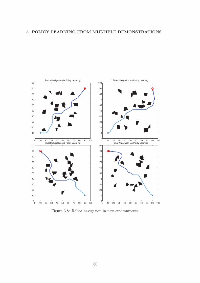
3. POLICY LEARNING FROM MULTIPLE DEMONSTRATIONS
0 10 20 30 40 50 60 70 80 90 1000
10
20
30
40
50
60
70
80
90
100Robot Navigation via Policy Learning
0 10 20 30 40 50 60 70 80 90 1000
10
20
30
40
50
60
70
80
90
100Robot Navigation via Policy Learning
0 10 20 30 40 50 60 70 80 90 1000
10
20
30
40
50
60
70
80
90
100Robot Navigation via Policy Learning
0 10 20 30 40 50 60 70 80 90 1000
10
20
30
40
50
60
70
80
90
100Robot Navigation via Policy Learning
Figure 3.8: Robot navigation in new environments.
60

3.6 Experimental Results
3.6.3 Paths Comparison
Since the paths are not the optimal ones, we are now investigating the differencebetween them. Given an unknown world, we first plan an optimal path in redcurve using our modified A* algorithm in a global view, and then let the robotnavigate by the learned policy. Figure 3.9 tells that the robot has learned tofind a quasi-optimal path unless sometimes it thinks dangerous to pass througha narrow path between obstacles, such as in the last navigation map. Also, aftertraining the robot, the robot can save much time in real-time navigation.
The robot may not always choose a similar path as the expert suggests, asthe last two figures in Figure 3.9. However, the robot could still navigate to thetarget without any collisions.
3.6.4 Autonomous Navigation in Dynamic Environments
We tested our policy learning algorithm in dynamic environments. The resultsare shown in Figure 3.10. In the environment, the black solid objects are staticobstacles, and the purple rectangle ones are moving obstacles, which move in anunpredictable direction.
The robot first encountered a static obstacle at time 10, after avoiding it,the robot encountered several moving obstacles around him at time 23. Therobot could successfully avoid them. Before arriving at the destination, the robotmet another moving obstacle at time 47, and he kept a safe distance with it.Finally the robot reached the destination without any collisions. Therefore, therobot has successfully learned an control policy from the expert demonstrationin autonomous navigation in dynamic environments.
3.6.5 Discussions
We compare the results if providing different number of demonstrations.
Number of demos 20 25 30 35 40Rate of success 89% 92% 92% 93% 94%
Table 3.2: Compassion of number of demonstration versus rate of success.
61

3. POLICY LEARNING FROM MULTIPLE DEMONSTRATIONS
0 10 20 30 40 50 60 70 80 90 1000
10
20
30
40
50
60
70
80
90
100Comparison in Robot Navigation
Elapsed time of modified A* : 8.0752 seconds.0 10 20 30 40 50 60 70 80 90 100
0
10
20
30
40
50
60
70
80
90
100Comparison in Robot Navigation
Elapsed time of modified A* : 24.2135 seconds.
0 10 20 30 40 50 60 70 80 90 1000
10
20
30
40
50
60
70
80
90
100Comparison in Robot Navigation
Elapsed time of Modified A* : 72.9017 seconds.0 10 20 30 40 50 60 70 80 90 100
0
10
20
30
40
50
60
70
80
90
100Comparison in Robot Navigation
Elapsed time of modified A* : 40.0755 seconds.
0 10 20 30 40 50 60 70 80 90 1000
10
20
30
40
50
60
70
80
90
100Comparison in Robot Navigation
Elapsed time of modified A* : 11.4812 seconds.0 10 20 30 40 50 60 70 80 90 100
0
10
20
30
40
50
60
70
80
90
100Comparison in Robot Navigation
Elapsed time of modified A* : 55.4684 seconds.
Figure 3.9: Path comparison in two methods. The red dotted curves are thesuggested paths by computer expert, and The blue solid curves are actual robotnavigation trajectories.
62

3.6 Experimental Results
Figure 3.10: Autonomous robot navigation in a dynamic environment using pro-posed policy learning method.
63

3. POLICY LEARNING FROM MULTIPLE DEMONSTRATIONS
We can see the rate of success change not that big, therefore, we can safelychoose a number of demonstrations of 25.
We also give the results how the different numbers of iterations in backprop-agation would influence the training performance.
Number of iterations 100 200 250 300 350 400 500Prediction accuracy(%) 81.12 82.68 82.83 83.62 83.31 83.15 83.46
Training time (s) 3.42 6.82 8.75 10.64 12.77 13.64 17.08
Table 3.3: Compassion of number of iterations in training performance.
Using the same training set, we can see that from 250 iterations, the predictionaccuracy stayed stable while the training time increased, and also more iterationswould risk overfitting. Therefore, a number of iterations between 250 and 350was a good choice.
From the above experiments, the robot successfully reproduces the task afterlearning a policy even when all objects are in novel positions. The proposedmethod using learning from demonstration has equipped a mobile robot withintelligence and adaptive abilities in performing an independent navigation task.
3.7 Conclusion
Building robust and reliable autonomous navigation systems that generalize acrossenvironments and operating scenarios remains a core challenge in robotics. Ourmotivation is for robot capabilities to be more easily extended and adapted tonovel situations, even by users without programming ability.
Learning from demonstration is an approach aimed at recovering the instruc-tions directly from teacher’s demonstrations.
In our work, we proposed a method for mobile robots to learning an optimalpolicy offline from expert demonstrations, especially in the cases where humandemonstrations are not available to obtain, and then to navigate online newenvironments autonomously. The neural network is applied to generalize theundemonstrated states. The experiments showed a good learning efficiency andgeneralization capability without lots of examples, and can eventually enable amobile robot to learn a policy to autonomously execute future navigation tasks.
64

Chapter 4
Reinforcement Learning underStochastic Policies
Contents4.1 Introduction . . . . . . . . . . . . . . . . . . . . . . . . 66
4.2 Related Work . . . . . . . . . . . . . . . . . . . . . . . . 67
4.3 Model-Free Reinforcement Learning Methods . . . . 69
4.3.1 Q-Learning . . . . . . . . . . . . . . . . . . . . . . . . 70
4.3.2 SARSA . . . . . . . . . . . . . . . . . . . . . . . . . . 71
4.3.3 Function Approximation using Feature-Based Repre-sentations . . . . . . . . . . . . . . . . . . . . . . . . . 72
4.4 Neural Network based Q-Learning . . . . . . . . . . . 73
4.4.1 State and Action Spaces . . . . . . . . . . . . . . . . . 74
4.4.2 Reward Function . . . . . . . . . . . . . . . . . . . . . 76
4.4.3 The Stochastic Control Policy . . . . . . . . . . . . . . 77
4.4.4 State-Action Value Iteration . . . . . . . . . . . . . . . 78
4.4.5 Algorithm . . . . . . . . . . . . . . . . . . . . . . . . . 81
4.5 Experimental Results . . . . . . . . . . . . . . . . . . . 83
4.5.1 Self-learning Results . . . . . . . . . . . . . . . . . . . 84
4.5.2 Autonomous Navigation Results . . . . . . . . . . . . 89
4.5.3 Comparison and Analysis . . . . . . . . . . . . . . . . 89
4.5.4 Autonomous Navigation in Dynamic Environments . . 91
65

4. REINFORCEMENT LEARNING UNDER STOCHASTICPOLICIES
4.5.5 Discussions . . . . . . . . . . . . . . . . . . . . . . . . 91
4.6 Conclusion . . . . . . . . . . . . . . . . . . . . . . . . . . 93
4.1 Introduction
Endowing robots with human-like abilities to perform specific skills in a smoothand natural way is one of the important goals of robotics. In the previous chapter,we investigated that a mobile robot learned a control policy via multiple expertdemonstrations. These demonstrations provided the robot with prior experienceand our learning algorithm generalized to the undemonstrated states. However,in some cases, such as exploring hazardous environments, no prior experience ordemonstrations are available to the mobile robots, and we still want them to learnhow to behave in unknown environments. This is the main problem that we aredealing with in this chapter.
Reinforcement learning (RL) is the key tool that helps us to create robotsthat can learn new skills by themselves, just similarly to our human beings.Reinforcement learning is realized by interacting with an environment. In RL,the learner is a decision-making agent that takes actions in an environment andreceives an reinforcement signal for its actions in trying to accomplish a task.The signal, well known as reward (or penalty), evaluates an action’s outcome,and the agent seeks to learn to select a sequence of actions, i.e. a policy, thatmaximize the total accumulated reward over time.
Reinforcement learning can be formulated as a Markov Decision Process.Model-based RL algorithms can be used if we know the state transition func-tion T (s, a, s′). In contrast, we focus more on model-free RL that the environ-ment model T is not known in advance, especially in our work of autonomousnavigation tasks.
The whole learning scenario is a process of trial-and-error runs. We applya Boltzmann probability distribution to tackle the problem of the exploration-exploitation tradeoff, that is, the dilemma between should we exploit the pastexperiences and select the actions that as far as we know are beneficial, or shouldwe explore some new and potentially more rewarding states. Under the circum-stances, the policies are stochastic.
66

4.2 Related Work
Classic RL algorithms are usually applied to small sets of states and actions,that is, the agent can only visit a subset of the of states during the trial-and-errorruns. In real applications, the state spaces are of a large scale and this will bringthe problems of the generalization and the curse of dimensionality. We use theneural network structure to generalize and approximate the value of all the states.In the previous chapter, we have successfully implemented the neural network totrain offline a control policy for mobile robots after all the state-action pairs arecollected. In this chapter, we use the network to do incremental online learningwithout acquiring the output labels explicitly.
In this chapter, we present a RL based self-learning algorithm in the caseswhere expert demonstrations cannot provided to learning agents in advance andthey need to find a robust policy via interacting with the environment (Xia &El Kamel, 2014a,c, 2015d). Experiments are conducted on the autonomous nav-igation tasks for mobile robots.
4.2 Related Work
Many researches on robot autonomous navigation using reinforcement learningwere conducted. In general, reinforcement learning is realized by the interactionbetween the robot and the surrounding environment. Instead of explicitly detail-ing the solution to a problem, in RL, the designer provides feedback that measuresthe one-step performance of the robotic system for future self-improvement.
Yang et al. (2004) used continuous Q-learning algorithm for solving the au-tonomous navigation problem for mobile robots. They used a multilayer feed-forward neural network to approximate the Q-learning value function. Thismethod designed only three actions and was applied for static environments.Also, the robot was trained in the same environment, and no proof of the porta-bility of the algorithm in other environments was provided.
Lagoudakis & Parr (2003) proposed the least-squares policy iteration (LSPI)that is motivated by the least-squares temporal-difference learning algorithm(LSTD) for prediction problems. This method can be efficiently used on batch re-inforcement learning problems. Also for batch learning, neural fitted-Q iteration(NFQ) (Riedmiller, 2005) is a model-free, neural network based reinforcementlearning algorithm to train Q-value functions. The main drawback of batch RL is
67

4. REINFORCEMENT LEARNING UNDER STOCHASTICPOLICIES
that it relys on the efficiency of a complete data collection, which is quite costly,
especially when the agent cannot achieve its goal in the learning scenarios.
Similar methods using reinforcement learning and neural network were pre-
sented in (Huang et al., 2005; Li et al., 2006; Qiao et al., 2008). These papers
have demonstrated the feasibility of their algorithms, but they share some com-
mon problems. First, these papers used exactly the same environment both to
train the robot learning ability and to test the navigation skills. However, what
is expected is that the robot learns the obstacle avoidance behaviors in some
environments and can navigate independently in a completely new unknown en-
vironment. Therefore, the robustness of their methods need to be proved. Second,
limited number of state and action spaces and simple design for reward function
bring the question of functionality of navigation tasks in more complicated envi-
ronments. Moreover, the algorithms in (Huang et al., 2005; Li et al., 2006) were
tested in static environments and only one dynamic obstacle was considered in
(Qiao et al., 2008).
Knudson & Tumer (2011) evaluated reactive and learning navigation algo-
rithms for exploration robots and showed a better performance using neuro-
evolutionary algorithm compared to rule-based algorithm. At the same time,
they indicated that when the environments became particularly complex, the
neuro-evolutionary algorithm was not able to establish a good policy for naviga-
tion.
Reinforcement learning are widely used in various robotic systems. A hu-
manoid robot navigation was described in (Navarro-Guerrero et al., 2012) by
using a supervised RL approach combined with Gaussian distributed state ac-
tivation, and the robot successfully performed a backward docking movement
used for autonomous recharging. El-Fakdi & Carreras (2013) proposed a two-
step gradient-based reinforcement learning control system for solving the action
selection problem of an autonomous underwater vehicle in a visual-based cable
tracking task. A neural network reinforcement learning method was studied for
visual control of a robot manipulator (Miljković et al., 2013). A direct mapping
from the image space to the actuator command was developed by using two dif-
ferent RL algorithms, Q-learning and SARSA, combined with neural networks. A
database of representative learning samples was also employed in order to speed
68

4.3 Model-Free Reinforcement Learning Methods
up the convergence of the algorithms. This hybrid system could provide a highaccuracy of a manipulator positioning in a situation of low resolution images.
Q-learning and SARSA algorithms are two major RL techniques, but theypossess different characteristics. SARSA has a faster convergence characteristics,while Q-learning has a better final performance. However, SARSA is easily stuckin the local minimum and Q-learning needs longer time to learn. Wang et al.proposed a method of combining Q-learning and SARSA algorithm, called back-ward Q-learning, to deal with the dilemma between exploration and exploitationfor action selection policy (Wang et al., 2013). This method can enhance learningspeed and improve the final performance. Moldovan and Abbeel also addressed amethod of safe exploration in Markov decision process when in uncertain dynamicenvironments (Moldovan & Abbeel, 2012).
Many other RL-related algorithms can be found in (Wiering & van Otterlo,2012). Xu et al. (2014) presents also a comprehensive survey on recent develop-ments in reinforcement learning algorithms with function approximation.
4.3 Model-Free Reinforcement Learning Methods
In our work, We study reinforcement learning and robot control problems inwhich a mobile robot acts in a stochastic environment by sequentially choosingactions over a sequence of time steps, in order to maximize a cumulative re-ward. We model the problem as a Markov Decision Process: a state space S,an action space A, a transition dynamics distribution P (st+1 | st, at) satisfyingthe Markov property P (st+1 | s1, a1, ..., st, at) = P (st+1 | st, at), for any trajectorys1, a1, s2, a2, ..., sT , aT in state-action space, and a reward function r : S ×A −→R. A stochastic policy π(st, at) = P (at | st) is used to select actions and producea trajectory of states, actions and rewards s1, a1, r1, s2, a2, r2, ..., sT , aT , rT overS ×A× R.
An on-policy method learns the value of the policy that is used to makedecisions. The value functions are updated using results from executing actionsdetermined by some policy. An off-policy methods can learn the value of theoptimal policy independently of the agent’s actions. It updates the estimatedvalue functions using hypothetical actions, those which have not actually beentried.
69

4. REINFORCEMENT LEARNING UNDER STOCHASTICPOLICIES
We focus on model-free RL methods that the robot drives an optimal policywithout explicitly learning the model of the environment. Q-learning (Watkins,1989) and Sarsa (Rummery & Niranjan, 1994) algorithms are two major model-free reinforcement learning algorithms.
4.3.1 Q-Learning
Q-Learning algorithm is an important off-policy model-free reinforcement learningalgorithm for temporal difference learning. It can be proven that given sufficienttraining under any ε-soft policy, the algorithm converges with probability 1 to aclose approximation of the action-value function for an arbitrary target policy.Q-Learning learns the optimal policy even when actions are selected according toa more exploratory or even random policy.
The update of state-action values in Q-learning is defined by
Q(st, at) := Q(st, at) + α[rt+1 + γmax
aQ(st+1, a)−Q(st, at)
]. (4.1)
The parameters used in the Q-value update process are:
α - the learning rate, set between 0 and 1. Setting it to 0 means that theQ-values are never updated, hence nothing is learned. Setting a high valuesuch as 0.9 means that learning can occur quickly.
γ - discount factor, also set between 0 and 1. This models the fact thatfuture rewards are worth less than immediate rewards. Mathematically, thediscount factor needs to be set less than 0 for the algorithm to converge.
In this case, the learned action-value function, Q, directly approximates Q∗,the optimal action-value function, independent of the policy being followed. Thisdramatically simplifies the analysis of the algorithm and enabled early conver-gence proofs. The policy still has an effect in that it determines which state-action pairs are visited and updated. However, all that is required for correctconvergence is that all pairs continue to be updated. Under this assumption anda variant of the usual stochastic approximation conditions on the sequence ofstep-size parameters, Qt has been shown to converge with probability 1 to Q∗.The Q-learning algorithm is shown below.
70

4.3 Model-Free Reinforcement Learning Methods
Algorithm 5 One-step Q-learning algorithm (Watkins, 1989)1: Initialize Q(s,a) arbitrarily;2: repeat(for each episode):3: Initialize s;4: repeat(for each step of episode):5: Choose a from s using policy derived from Q;6: Take action a, observe r, s′;7: Q(s, a) ← Q(s, a) + α [r + γmaxa′ Q(s′, a′)−Q(s, a)];8: s ← s′;9: until s is terminal
10: until all episodes end.
4.3.2 SARSA
The SARSA algorithm is an on-policy algorithm for TD-Learning. The major
difference between it and Q-Learning, is that the maximum reward for the next
state is not necessarily used for updating the Q-values. Instead, a new action, and
therefore reward, is selected using the same policy that determined the original
action. The name SARSA actually comes from the fact that the updates are done
using the quintuple Q(s, a, r, s′, a′). Where: s, a are the original state and action,
r is the reward observed in the following state and s′, a′ are the new state-action
pair. The Q-value update rule is defined by
Q(st, at) := Q(st, at) + α [rt+1 + γQ(st+1, at+1)−Q(st, at)] (4.2)
It is straightforward to design an on-policy control algorithm based on the
SARSA prediction method. As in all on-policy methods, we continually estimate
Qπ for the behavior policy π, and at the same time change π toward greediness
with respect to Qπ. The general algorithm is given as:
As you can see, there are two action selection steps needed, for determining
the next state-action pair along with the first. The parameters α and γ have the
same meaning as they do in Q-Learning.
71

4. REINFORCEMENT LEARNING UNDER STOCHASTICPOLICIES
Algorithm 6 On-policy SARSA algorithm (Rummery & Niranjan, 1994)1: Initialize Q(s,a) arbitrarily;2: repeat(for each episode):3: Initialize s;4: Choose a from s using policy derived from Q;5: repeat(for each step of episode):6: Take action a, observe r, s′;7: Choose a′ from s′ using policy derived from Q;8: Q(s, a) ← Q(s, a) + α [r + γQ(s′, a′)−Q(s, a)];9: s ← s′; a ← a′;
10: until s is terminal11: until all episodes end.
4.3.3 Function Approximation using Feature-Based Repre-sentations
For problems with high dimensionality, the number of states become astronom-ically large making Q-value table storage infeasible. So the practical implemen-tation of Q-Learning requires using Q-value approximation via generalization ofstates, i.e., features.
Features are functions from states to real numbers that capture importantproperties of the state. Using a feature representation, we can write a Q-function(or value function) for any state using a few weights:
V (s) = ω1f1(s) + ω2f2(s) + ...+ ωnfn(s)
Q(s, a) = ω1f1(s, a) + ω2f2(s, a)...+ ωnfn(s, a)
By this representation, our experience can be summed up in a powerful num-bers. However, states may share features but actually be very different in value.
In robotics, it’s often usually to use linear or non-linear feature representationsto handle the large-scale state-action spaces.
SARSA with Linear Function Approximation
You can use a linear function of features to approximate the Q-function inSARSA. This algorithm uses the on-policy method SARSA, because the agent’sexperiences sample the reward from the policy the agent is actually following,
72

4.4 Neural Network based Q-Learning
rather than sampling an optimum policy. A number of ways are available to geta feature-based representation of the Q-function. In this section, we use featuresof both the state and the action to provide features for the linear function.
Suppose {f1, ..., fn} are numerical features of the state and the action. Thus,fi(s, a) provides the value for the i-th feature for state s and action a. These fea-tures are typically binary, with domain [0, 1], but they can also be other numericalfeatures. These features will be used to represent the Q-function.
Qω(s, a) = ω0 + ω1f1(s, a) + ...+ ωnfn(s, a) (4.3)
For some tuple of weights, ω = [ω0, ω1, ..., ωn]. Assume that there is an extrafeature f0 whose value is always 1, so that ω0 does not have to be a special case.
An experience in SARSA of the form {s, a, r, s′, a′} (the agent was in states, did action a, and received reward r and ended up in state s′, in which itdecided to do action a′) provides the new estimate of r + γQ(s′, a′) to updateQ(s, a). This experience can be used as a data point for linear regression. Letδ = r + γQ(s′, a′)−Q(s, a). Weight ωi is updated by
ωi ←− ωi + αδfi(s, a).
This update can then be incorporated into SARSA, giving the algorithm 7.Similarly, we can use linear function approximation on Q-learning algorithm.
The transition is of the form {s, a, r, s′}, and the difference
δ =[r + γmax
a′Q(s′, a′)
]−Q(s, a).
The update rules for Q-values and weights are:
Q(s, a) ←− Q(s, a) + αδ;
ωi ←− ωi + αδfi(s, a).
4.4 Neural Network based Q-Learning
In this section we present our contribution that incorporating a neural networkto Q-learning. One of the strengths of Q-learning is that it is able to compare
73

4. REINFORCEMENT LEARNING UNDER STOCHASTICPOLICIES
Algorithm 7 SARSA with linear function approximation (Poole & Mackworth,2010)
Input:f = [f1, ..., fn]: a set of features;γ ∈ [0, 1]: discount factor;α > 0: step size for gradient descent.
1: Initialize weights ω = [ω0, ω1, ..., ωn];2: Observe current state s;3: Select action a (stochastic policy π(a|s));4: repeat5: Carry out action a (transition probability Pr(s′|s, a));6: Observe state s′ and receive reward r;7: Select action a′ using a policy based on Qω (stochastic policy π(a′|s′));8: Let δ = r + γQ(s′, a′)−Q(s, a);9: for i = 0 to n do
10: Update weights: ωi ← ωi + αδfi(s, a);11: end for12: s ← s′, a ← a′;13: until Termination.
Output: An optimal weights ω∗.
the expected utility of the available actions without requiring a model of theenvironment. Q-learning can handle problems with stochastic transitions andrewards.
4.4.1 State and Action Spaces
Since reinforcement learning algorithms can be modeled as an MDP, we need firstto define the state space S and action space A.
Q-learning is aimed at learning a mapping from the state input to the actionoutput. In a navigation problem, the robot perceives the state from the environ-ment by means of its sensors, and this state of environment is used by a reasoningprocess to determine the action to execute in the given state.
The action space A is defined by six discrete robot actions. Among them, fiveare basic moving actions∗: move forward (F), turn left at 30◦ (L30), turn left at60◦ (L60), turn right at 30◦ (R30), turn right at 60◦ (R60) and one emergencyaction: move backward (B). The six actions are based on the robot heading
∗These five moving actions are defined as the same ones that we used in the previous chapter.
74

4.4 Neural Network based Q-Learning
orientation. A turn at 90◦ is not defined because a sharp turn will bring great
danger to a real vehicle. Moving backward is regarded as an emergency action
that is only executed when no path is available in front of the robot and whatever
turns cannot avoid obstacles. This action is not considered in the self-learning
process, because it is, in some sense, an ‘instinct’ behavior of mobile robots. In
sum,
A = {F, L30, L60, R30, R60, B}. (4.4)
The state space S = {S1, S2, S3, ..., SN} is composed of a very large but finite
number of states, and each state St is defined based on the 11-dimensional state
representation that we gave in Equation (3.17).
However, we do not consider the degrees of danger of the No.5 and No.6
sensors (see Figure 2.6) thanks to the instinct action ‘B’. This can help re-
duce the complexity of the computation of the dimensionality. Thus, Dt =
[d1, d2, d3, d4, d7, d8, d9]� ∈ R
7×1.
When a sensor detects an obstacle, a robot should distinguish if this obstacle
is an object that can be bypassed or a wall that cannot be bypassed. Hence, we
introduce a vector Ut ∈ R7×1 to indicate if a wall is detected (U = 1) or an object
obstacle (U = 0) for the seven sensors in Dt.
Therefore, a state can be defined by four groups of features, and is expressed
in:
St =
⎡⎢⎢⎢⎣Dt
Vt
It
Ut
⎤⎥⎥⎥⎦ ∈ R
16×1. (4.5)
Vt ∈ {1, 2, ..., 9} is the target region and It ∈ {0, 1} is the indicator that
determines if the robot has detected the target.
Note: Since the robot needs to deal with different environments, and the robot
position coordinates have no direct relation with the target and the obstacles in
different environments, it is not necessary to include them as part of the state
features. The robot localization can be fixed by many methods and is not the
focus of this thesis, so we assume the robot know its position relative to its start
position.
75

4. REINFORCEMENT LEARNING UNDER STOCHASTICPOLICIES
4.4.2 Reward Function
The reward function measures the immediate feedback for the action taken at agiven state. It evaluates how good or how bad the performed action is. Beforegiving the reward function, one environment state at each time instant is classifiedinto four properties, called the state property pt:
One world state St is classified into five properties, called the state propertypt:
• Safe State (SS): a state where no surrounding obstacles has been detected.
• Cozy State (CS): a state where the robot has a low or no probability ofcollision with surrounding obstacles.
• Dangerous State (DS): a state where the robot has a high probability ofcollision with some obstacles in the environment.
• Winning State (WS): a terminate state where the robot reaches its target.
• Failure State (FS): a terminate state where the robot collides with obstacles.
pt =
⎧⎪⎪⎪⎪⎪⎪⎪⎨⎪⎪⎪⎪⎪⎪⎪⎩
SS, dbou ≤ dr−o
CS, dcozy ≤ dr−o ≤ dbou
DS, dcol ≤ dr−o ≤ dcozy
WS, dr−t ≤ dwin
FS. dr−o ≤ dcol
(4.6)
dr−o and dr−t define the distances between the robot and obstacles, and thetarget. dbou defines the boundary distance (sensor detection range) of SS andother states. dcol defines the radius of the collision region around the obstacle.dwin defines the radius of the winning region around the target. dcozy defines thecozy distance. These distances can be found in Figure 2.7.
Based on the state properties, the reward function r(t) is defined in Table 4.1.
dt−1min and dtmin are the minimum distances between the robot and the sur-
rounding obstacles respectively at instant t− 1 and instant t. dwarn is a warningdistance that the robot is approaching too close to an obstacle.
76

4.4 Neural Network based Q-Learning
State Transition Extra Criteria r
other states → Winning State 1Safe State → Cozy State 0Cozy State → Safe State 0
Dangerous State → Cozy State 0.5Cozy State → Dangerous State 0
Dangerous State → Failure State -1dwarn ≤ dtmin ≤ dt−1
min − 2 -0.2Dangerous State → Dangerous State dtmin = dt−1
min − 1 ≤ dwarn -0.2(approaching obsacles) dtmin = dt−1
min − 2 ≤ dwarn -0.5dtmin ≤ dt−1
min − 3 -1Nonsafe State → Nonsafe State dwarn ≤ dtmin 0.6
(evading obstacles) dtmin ≥ dwarn 0.4
Table 4.1: Reward Function
4.4.3 The Stochastic Control Policy
A reinforcement learning agent learns from the consequences of its state-actionpairs rather than from being explicitly taught, and it selects its actions on basisof its past experiences and also by new choices. If we may visit each state-action(s, a) a sufficient large number of times, we could obtain the state values via,for example, Monte Carlo methods. However, it is not realistic, and even worse,many state-action pairs would not be visited once. It is important to deal withthe exploration-exploitation tradeoff.
In our work, we transplant a Boltzmann distribution to express a stochasticcontrol policy. The learning agent tries out actions probabilistically based ontheir Q-values. Given a state s, the stochastic policy outputs an action a withprobability:
π(s, a) = P (a | s) = eQ(s,a)
T∑b∈A e
Q(s,b)T
. (4.7)
where T is the temperature that controls the stochasticity of action selection.If T is high, all the action Q-values tend to be equal, and the agent choosea random action. If T is low, the action Q-values differ and the action withthe highest Q-value is preferred to be picked. Thus, P (a|s) ∝ e
Q(s,a)T > 0 and
77

4. REINFORCEMENT LEARNING UNDER STOCHASTICPOLICIES
∑a P (a|s) = 1.We do not fix the temperature to a constant, since random exploration through-
out the whole self-learning process takes too long to focus on the best actions.At the beginning, all Q(s, a) are generated inaccurately, so a high T is set to
guarantee the exploration that all actions have a roughly equal chance of beingselected. As time goes on, a large amount of random exploration have beendone, and the agent could gradually exploit its accumulating knowledge. Thus,the agent decreases T , and the actions with the higher Q-values become moreand more likely to be picked. Finally, as we assume Q is converging to Q∗, Tapproaches zero (pure exploitation) and we tend to only pick the action with thehighest Q-value:
P (a|s) ={
1, if Q(s, a) = maxb∈A Q(s, b)
0, otherwise(4.8)
In sum, the agent starts with high exploration and converts to exploitation astime goes on, so that after a while we are only exploring (s, a)’s that have workedout at least moderately well before.
4.4.4 State-Action Value Iteration
The Q-value function expresses the mapping policy from the perceived state ofenvironment to the executing action. One Q-value Q(st, at) corresponds with onespecific state and one action in this state. Autonomous navigation tasks are ourmain research problems. Like many robotic applications in real life, they have alarge-scale state and action spaces. Traditionally, all the state or action values arestore in a Q-table. However, this is not practical and computationally expensivefor large-scale problems. In our method, We propose to predict all state Q-valuesby using a three-layer neural network, as shown in Figure 4.1.
The inputs are the state features that the robot perceives in the surroundingenvironment, and the outputs correspond to all the action Q-values. Therefore,according to Equations (4.4) and (4.5), the network has 16 neurons in the inputlayer, and 5 in the output layer∗. Moreover, 8 neurons are designed in the hiddenlayer.
∗Remember that the action ’B’ is an instinctive action that we do not need to learn, so onlythe other five actions are considered in the output layer.
78

4.4 Neural Network based Q-Learning
��
�"
��
��
&�
&�
&�
&�
' ��� ����
' ��� ����
' ��� ����
' ��� ����
"�� �#����$���%���
& ����'�!%��
�� ��( ��� ( ���
�����
Figure 4.1: A three-layer neural network architecture.
The bias units are set to 1. The weight W (1) ∈ R8×17 is used to connect the
input layer and the hidden layer, and similarly, the weight W (2) ∈ R5×9 links the
hidden layer and the output layer. The sigmoid function is used for calculating
the activations in the hidden and output layers.
We denote Q(st) a vector of all action-values in the state st, and use Q(st, at)
to specify the Q-value of taking at in st. Thus,
Q(st) =
⎡⎢⎢⎢⎢⎢⎢⎣
Q(st, a1)
Q(st, a2)
Q(st, a3)
Q(st, a4)
Q(st, a5)
⎤⎥⎥⎥⎥⎥⎥⎦.
The action value iteration is realized by updating the neural network by the
means of its weights. In the previous chapter, the neural network was applied
for supervised learning where the label for each training state-action pair was
explicitly provided. Differently, the neural network in the reinforcement learning
does not has label outputs. Q-learning is a process of value iteration and the
optimal value after each iteration serves as the target value for neural network
training. The update rule is
79

4. REINFORCEMENT LEARNING UNDER STOCHASTICPOLICIES
Qk+1(st, at) = Qk(st, at) + α
[rt + γmax
a∈AQk(st+1, a)−Qk(st, at)
]. (4.9)
where the initial action values Q0 of al the state-action pairs are generated ran-
domly between 0 and 1. Qk+1(st, at) is treated as the target value of the true
value Qk(st, at) in the (k + 1)th iteration.
In the vector Qk(st), only Qk(st, at) is updated to Qk+1(st, at), and the rest
elements stay unchanged. Sometimes, Qk+1(st, at) may exceed the range [0, 1],
then we need to rescale Qk+1(st) to make sure all its components are in [0, 1].
We denote Qk+1(st) the rescaled action value. To make it clear, the update of
Q-value is realized along the road Qk → Qk+1 → Qk+1.
The network error is a vector of form:
δk+1 = Qk+1(st)−Qk(st). (4.10)
We employ the stochastic gradient descent (SGD) to train the neural network
online. The goal is to minimize the cross-entropy cost function J defined as:
J = −[
NA∑i=1
(Qk+1)i · log(Qk)i + (1− (Qk+1)i)(1− log(Qk)i)
]. (4.11)
where NA is the number of actions used for training. In our navigation tasks,
NA = 5.
The action Q-values are nonlinear functions of weights of the network. SGD
optimizes J and updates weights by using one or a few training examples accord-
ing to:
W (i) ← W (i) − σ∂J
∂W (i). (4.12)
Each iteration outputs new weights W (i) and a new cost J ′ is calculated. This
update repeats until it arrives at a maximum times of iteration or |J ′ − J | < ε.
80
4.4 Neural Network based Q-Learning
4.4.5 Algorithm
An autonomous navigation tasks via NNQL can be divided into two processes.The first one is the training process to endow the robot with the self-learningability, and the second one is the navigation process to use the trained policy toexecute an independent navigation task (Xia & El Kamel, 2015d).
4.4.5.1 Training Process of NNQL
Training the mobile robot is done by exposing it to a bunch of learning episodesand each episode has a different environment. Also, the robot has a set of initialstarting positions. The variety helps the robot to encounter as many situationsas possible, which could accelerate the learning speed.
Each episode starts by perceiving the current state of the environment. Therobot detects the surrounding obstacle locations through its sensors, and a roughtarget region∗ is supplied to the robot. Once the current state is checked, if itis a Safe State, the robot executes a goal-oriented behavior that it changes itsorientation towards the target position, and moves one step forward trying toget closer. If the current state is Non-Safe State, the robot sends the currentstate features into the FFNN and outputs all the possible Q-values. According tothe action selection strategy represented by a stochastic control policy, the robotpicks an action and moves to a new state. Then, the robot checks the resultingnew state, receives the immediate reward and updates the Q-values accordingly.Then the updated Q-values are sent back to the neural network and use thebackpropagation algorithm to update the weights of the network.
Each episode has a limited amount of moving steps. The robot needs to reachthe target within the steps. If the robot runs out of the steps and does not reachthe target, or if the robot collides with an obstacle or reach the target, the episodeis terminated and a new episode is started.
The key of training efficiency is greatly related to how to make use of theaccumulated sequence of state-action pairs and their Q-values. A bunch of pre-vious work (Jaradat et al., 2011; Qiao et al., 2008; Xia & El Kamel, 2015d) usedone-step Q-learning to update one Q-value at a time. When the robot arrives at
∗“A rough target region” means that the robot only knows in which sensor region locatesthe target, but has no idea of the exact direction and the relative distance between itself andthe target. This concept was also presented in Equation (4.5).
81

4. REINFORCEMENT LEARNING UNDER STOCHASTICPOLICIES
a new state, only the new Q-value will be updated and the previous action valueswill be discarded. Others used batch learning (Riedmiller, 2005) that updatesall the Q-values once they are all collected. This also poses some advantages.First, without online update, we cannot guarantee that the collected Q-valueshave their optimal target values. Moreover, waiting all the values being obtainedis always time-wasting. We propose to update online not only the current Q-valuebut also gather the previous values to train together.
The training algorithm is given in Algorithm 8.
Algorithm 8 Training algorithm of NNQL1: Initialize the NN weights W (1) and W (2) randomly;2: for all episodes do3: Give the target and generate obstacles randomly;4: Load the robot initial position [x0, y0] and orientation θ0;5: Observe current state s1 and state property p1;6: input := [ ], target := [ ];7: t ← 1;8: for all moving steps do9: Compute all action-values {Q(st, ai)}i in state st via NN;
10: Select one action at according to the stochastic policy π(s, a) in (4.7),and then move;
11: Observe new state st+1 and state property pt+1;12: Obtain the immediate reward rt;13: Update the Q-value function from Q(st, at) to Q(st, at) via (4.9);14: Apply feature scaling for Q to the range [0, 1];15: Add st to input, and add Q(st, a) to target;16: Apply SGD to train (input, target) and to update the weights W (1)
and W (2);17: if st+1 is Winning State or Failure State then18: Start a new episode;19: end if20: t ← t+ 1;21: end for22: end for
4.4.5.2 Robot Navigation Using NNQL
After training the robot, the resulting policy is still stochastic but near-deterministicthat used by the robot for future navigation tasks in various environments.
82

4.5 Experimental Results
The robot starts its navigation through the environment by finding its currentstate. If it is a Safe State the robot does not need to follow the policy but changesits orientation towards the target and moves one step forward. It continues mov-ing until entering a Non-Safe region where the robot needs to adopt the trainedcontrol policy. The robot uses the FFNN to generate all possible state-actionQ-values. The robot greedily takes the action that has the biggest Q-value. Af-ter that, the robot finds its new state and repeats the process of action selectionuntil the robot reaches its goal or collide an obstacle. The navigation algorithmis shown in Algorithm 9.
Algorithm 9 Robot Navigation using NNQL1: Load the trained NN weights W (1) and W (2);2: Give the target and generate obstacles randomly;3: Load the robot initial position [x0, y0] and orientation θ0;4: t ← 1;5: for all moving steps do6: Observe current state st and state property pt;7: if st is Winning State or Failure State then8: Terminate the navigation;9: end if
10: Compute all action Q-values {Q(st, ai)}i via neural network;11: Pick the moving action at according to greedy policy, and then move;12: end for
4.5 Experimental Results
We employ the mobile robot model described in Chapter 2.5 to undertake au-tonomous navigation tasks in unknown environments.
The environment map has a size of 100×100 m2. The obstacles are randomlyscattered in the environment and the robot has no prior knowledge of their num-bers, sizes and positions. The initial positions of the robot (a blue solid rectanglein the map) is placed at (10, 10) or (90, 10). The target positions (a red hollowcircle in the map) may be found at (90, 90) or (10, 90). The velocity of the robotis fixed at 2.5 m/s. The mission of the robot is to start from the initial positionand to find an optimal path to arrive at the target position without any collision
83

4. REINFORCEMENT LEARNING UNDER STOCHASTICPOLICIES
with any obstacles. If no obstacles are detected, the robot is designed to stick toa goal-oriented behavior.
We use a 16-8-5 three-layer neural network to approximate all action Q-values.It is also used to generalize to unvisited states.
4.5.1 Self-learning Results
The self-learning process is conducted in a number of learning episodes, andeach episode has a maximum of 400 moving steps. All episodes have differentconfigurations of random obstacle positions. A new episode will be started in thefollowing three situations:
• The robot finds a collision free path to the target;
• The robot collides with an obstacle or the map borders;
• The robot runs out the moving steps.
The training process will be terminated when all the learning episodes arefinished. The experiment parameters are selected as follows:
• Learning rate of Q-function in Equation (4.9): α = 0.8,
• Discount factor of Q-function: γ = 0.7,
• Learning rate of SGD in Equation (4.12): σ = 0.3,
• Maximum temperature in Equation (4.7): Tmax = 0.9,
• Minimum temperature: Tmin = 0.9.
The learning results are shown in Figure 4.2.300 episodes are set for the robot to learn to navigate in different environ-
ments. One advantage of learning in different environments is that the robot canalways face new challenge and avoid falling into infinite loops when it gets used ofits environment. We can see that the robot tried different actions and the rewardsevaluated this action decision, which can help the robot to correct the action se-lection in the future. During all episodes, the proposed algorithm adopted BPNNto train the weights W (1) and W (2). When the learning process is completed, the
84

4.5 Experimental Results
0 10 20 30 40 50 60 70 80 90 1000
10
20
30
40
50
60
70
80
90
100Learning Episode: 10
0 10 20 30 40 50 60 70 80 90 1000
10
20
30
40
50
60
70
80
90
100Learning Episode: 20
0 10 20 30 40 50 60 70 80 90 1000
10
20
30
40
50
60
70
80
90
100Learning Episode: 40
0 10 20 30 40 50 60 70 80 90 1000
10
20
30
40
50
60
70
80
90
100Learning Episode: 70
0 10 20 30 40 50 60 70 80 90 1000
10
20
30
40
50
60
70
80
90
100Learning Episode: 90
0 10 20 30 40 50 60 70 80 90 1000
10
20
30
40
50
60
70
80
90
100Learning Episode: 100
Figure 4.2: Learning results in different episodes via NNQL.
85

4. REINFORCEMENT LEARNING UNDER STOCHASTICPOLICIES
weights have been well trained and can be used directly in the following process
of robot navigation. Since the proposed algorithm is a trial-and-error method, it
is reasonable that a great number of episodes failed due to a collision.
0 50 100 150 200 250 300
−0.05
−0.04
−0.03
−0.02
−0.01
0
0.01
0.02Changes of W(1) in all learning episodes
episode
(a) Changes of W (1) in all learning episodes
0 50 100 150 200 250 300
−0.03
−0.02
−0.01
0
0.01
0.02
0.03
0.04
0.05
0.06
0.07Changes of W(2) in all learning episodes
episode
(b) Changes of W (2) in all learning episodes
Figure 4.3: Changes of NN weights in all learning episodes.
We measured the changes of the weights of the network in Figure 4.3. The
change in one episode is computed by the difference between the weight at the
beginning of the episode W (i) and the weight at the end of the episode ˜W (i):
86

4.5 Experimental Results
ΔW (i) =∑j
∑k
(˜w(i)j,k − w
(i)j,k
).
The figures showed that both of the weights fluctuated strong in the beginning
episodes and then went quiet around 0 after 100 episodes. The overall trend of
weight changes was turning stable as the learning process carried on and the
weights converged to their optimal values. That is to say, the robot has gradually
learned how to cope with the surrounding environment.
The numbers of successful learning in every 100 episodes is shown in Figure
4.4.
1 2 3 4 5 6 7 8 9 100
2
4
6
8
10
12
14
16Total Successful Episodes
No.
Every 30 episodes
Figure 4.4: Numbers of successful learning episodes in every 30 episodes.
A successful learning is an episode in which the robot succeeds in arriving
at the target position. In the first 100 episodes, less than 10 were successful,
but in the last 100 episodes, more than 60 witnessed the robot arriving at the
target. This remarkably increasing trend demonstrated that the proposed NNQL
algorithm helped the robot to become intelligent.
87

4. REINFORCEMENT LEARNING UNDER STOCHASTICPOLICIES
0 10 20 30 40 50 60 70 80 90 1000
10
20
30
40
50
60
70
80
90
100Robot Navigation via NNQL
0 10 20 30 40 50 60 70 80 90 1000
10
20
30
40
50
60
70
80
90
100Robot Navigation via NNQL
0 10 20 30 40 50 60 70 80 90 1000
10
20
30
40
50
60
70
80
90
100Robot Navigation via NNQL
0 10 20 30 40 50 60 70 80 90 1000
10
20
30
40
50
60
70
80
90
100Robot Navigation via NNQL
0 10 20 30 40 50 60 70 80 90 1000
10
20
30
40
50
60
70
80
90
100Robot Navigation via NNQL
0 10 20 30 40 50 60 70 80 90 1000
10
20
30
40
50
60
70
80
90
100Robot Navigation via NNQL
Figure 4.5: Autonomous navigation results in different environments via NNQL.
88

4.5 Experimental Results
4.5.2 Autonomous Navigation Results
In the navigation process, the weights W (1) and W (2) have converged to theiroptimal values. The robot has learned how to behave in front of obstacles. TheFFNN is now only adopted, and the robot chooses the best fit action. Then itis the time for the mobile robot to demonstrate its intelligence of independentnavigation in an unexpected environment.
Figure 4.5 showed six completely new navigation missions using the sameweights. The robot tried from different start points to reach different targetpositions. The robot succeeded in getting to the target position in a collision-freepath in all four environments and the robot always kept a safe distance to thesurrounding obstacles.
It is observed that the paths that the robot chose may not be the optimalones due to a lack of complete knowledge of environment map, but they are stillfully acceptable and perfect enough to meet our expectation, especially in suchcomplicated environments.
In order to test the robustness of the algorithm, we tried six different robotspeeds and for each speed we conducted 100 experiments. The results are shownin Table 4.2.
Robot speed (m/s) 1.5 2 2.5 3 3.5 4Rate of success (%) 100 100 100 97 94 90
Table 4.2: Compassion of the rate of success versus different robot speeds.
It is normal that a higher speed means a shorter reaction time, and thus astronger possibility of collision. These tests with different speeds achieved a highrate of success.
Therefore, the above experiments have proven the feasibility and the stabilityof the proposed NNQL algorithm.
4.5.3 Comparison and Analysis
For our study, we implement and compare several methods: the first one is ourproposed method NNQL; the second one is the online one-step Q-learning (onlineQL) that adopted in many previous work; the third one is the neural fitted-Q
89

4. REINFORCEMENT LEARNING UNDER STOCHASTICPOLICIES
iteration (NFQ), which is a successful batch learning method. We conducted 50times for each method.
Figure 4.6: Numbers of successful learning episodes in every 30 episodes.
Figure 4.6 showed the comparison of total successful learning in every 30episodes. The blue solid line is the average result of NNQL over 50 experiments,the red dashed line is the online QL method, and the green dash-dot line is NFQalgorithm. The shaded areas represent the standard derivation. We can see thatNNQL outperformed the other two popular methods. NFQ did not begin traininguntil all the training data had been collected, and hence it was easy to fail anepisode without adjusting its control policy. Online QL did the worst since this‘extravagant’ method abandoned so many training data and 300 episode was farfrom enough.
Let the mobile robot navigate autonomously in unknown environments afterbeing trained by those three methods. We fixed the robot velocity at 2.5 m/s anda total amount of 300 learning episodes. For each method we obtained 50 controlpolicies and for each policy we carried out 100 navigation tasks. The results werecompared in Table 4.3.
We can tell that our method achieved the best result, NFQ did slightly worse,and online QL needed more episodes to catch up with the performance.
90

4.5 Experimental Results
NNQL Online QL NFQAverage rate (%) 98 56 87
Best rate (%) 100 74 97Worst rate (%) 94 29 83
Table 4.3: Comparison of the rate of success versus different methods.
4.5.4 Autonomous Navigation in Dynamic Environments
We tested the NNQL algorithm in dynamic environments. The results are shown
in Figure 4.7. In the environment, the black solid objects are static obstacles,
and the purple rectangle ones are moving obstacles.
At time 31, the robot met some static obstacles around him, and successfully
avoid them. At time 50, before arriving at the destination, the robot found a
moving obstacle in front of him, and the robot successfully avoided it and finally
arrived at the destination. Therefore, NNQL has proven its feasibility in the
application of autonomous navigation in dynamic environments.
4.5.5 Discussions
From the above experiment results, NNQL has demonstrated good and reliable
performance in autonomous navigation tasks without explicitly programming
robot behaviors. With 300 episodes, which is not a big number, the robot can ex-
ecute an independent navigation with almost 100% confidence. Compared with
two popular model-free algorithms, NNQL outperformed them. We can safely
reach the conclusion that NNQL has successfully empowered a mobile robot with
strong self-learning ability in autonomous navigation tasks.
One limitation is that under stochastic policies, the path that the robot choose
may not be optimal, and the robot may wonder for a while in some place before
finding a way out. That is because the robot do not have a global view of the
environment and therefore has to explore the environment in order to memo-
rize a small range of the surrounding environment. One potential solution is to
incorporate simultaneous localization and mapping (SLAM) techniques.
91

4. REINFORCEMENT LEARNING UNDER STOCHASTICPOLICIES
Figure 4.7: Autonomous robot navigation in a dynamic environment usingNNQL.
92

4.6 Conclusion
4.6 Conclusion
Much of classical robotics focused on reasoning, optimal control and sensor pro-cessing given models of the robot and its environment. While this approach issuccessful for many industrial applications, it falls behind the more ambitiousgoal of robotics as a test platform for our understanding of artificial intelligence.
This chapter presented the robot self-learning strategy without prior experi-ence under explicit feedback. We explored the mobile robot navigation problemby combining reinforcement learning and neural network. Q-learning is appliedto enhance the self-learning ability of a mobile robot through trial-and-error in-teractions with an unknown environment. We designed new reward expressionand introduced the neural network architecture to store and train the large-scaleQ-values, and also to generalize the learning performance to large-scale state andaction spaces. The experiment results show the feasibility and the stability of theproposed method. The robot can complete navigation tasks safely in an unpre-dicted dynamic environment and becomes a truly intelligent system with strongself-learning and adaptive abilities.
93

4. REINFORCEMENT LEARNING UNDER STOCHASTICPOLICIES
94

Chapter 5
Learning Reward Functions withNonlinear Neural PolicyRepresentations
Contents5.1 Introduction . . . . . . . . . . . . . . . . . . . . . . . . 96
5.2 Related Work . . . . . . . . . . . . . . . . . . . . . . . . 98
5.3 Inverse Reinforcement Learning . . . . . . . . . . . . . 100
5.3.1 Preliminaries . . . . . . . . . . . . . . . . . . . . . . . 100
5.3.2 Inverse Reinforcement Learning . . . . . . . . . . . . . 101
5.4 Nonlinear Neural Policy Representations . . . . . . . 103
5.4.1 State and Action Spaces . . . . . . . . . . . . . . . . . 103
5.4.2 Neural Policy Representation . . . . . . . . . . . . . . 104
5.4.3 Stochasticity of Policy . . . . . . . . . . . . . . . . . . 106
5.5 Neural Inverse Reinforcement Learning . . . . . . . . 107
5.5.1 Suboptimal Demonstration Refinement via Maximuma Posteriori Estimation . . . . . . . . . . . . . . . . . 107
5.5.2 Model-free Maximum Margin Planning . . . . . . . . . 108
5.5.3 Neural Policy Iteration . . . . . . . . . . . . . . . . . . 109
5.5.4 The Algorithm for Neural Inverse Reinforcement Learning110
5.5.5 Expert Demonstrations . . . . . . . . . . . . . . . . . 112
95

5. LEARNING REWARD FUNCTIONS WITH NONLINEARNEURAL POLICY REPRESENTATIONS
5.6 Experimental results . . . . . . . . . . . . . . . . . . . 112
5.6.1 Comparison of Two Types of Demonstrations . . . . . 114
5.6.2 Neural Inverse Reinforcement Learning . . . . . . . . . 115
5.6.3 Robot navigation in new unknown environments . . . 118
5.6.4 Analysis of the weight changes . . . . . . . . . . . . . 120
5.6.5 Autonomous Navigation in Dynamic Environments . . 122
5.6.6 Discussions . . . . . . . . . . . . . . . . . . . . . . . . 123
5.7 Conclusion . . . . . . . . . . . . . . . . . . . . . . . . . . 124
5.1 Introduction
In this day and age, more and more robots are produced to assist or replace ourhuman beings to perform complicated planning and control operations and tasks,such as manipulating objects, navigating in outdoor environments, and drivingin urban areas. We are aware of the fact that designing such controllers for thesetasks is usually a complicated process, even for people specialized in programmingrobots, which requires creating by hand a new and different controller for eachparticular task. The designer has to take deliberately the wide range of situationsthat the robot may face into account. This sort of manually programming isgenerally an expensive as well as intense time-consuming process. Rather thanpre-programming a robot for all the tasks, it would be more useful if the robotcould learn such tasks by themselves.
In the previous chapter, we presented our reinforcement learning technique.In this framework, an learning robot interacts with a dynamic environment andfinds a policy through a reward function. This method was proven to be a power-ful and reliable solution to robot learning. However, one fundamental assumptionof successful RL algorithms is the reward function, the most succinct represen-tation of the designer’s intention, needs to be provided beforehand. In practice,defining the reward function can itself be a challenge because an informative re-ward function may be very hard to specify and exhaustive to tune for large andcomplex problems. The reward function we used in the previous chapter was notquite a straightforward one.
96

5.1 Introduction
People are wondering if we could extract a reward function from demonstratedexamples of a desired behavior, and this inspires the advent and the developmentof Inverse Reinforcement Learning (IRL). IRL can be taken as an extension ofreinforcement learning, which directly tackles the problems of learning a rewardfunction through expert demonstrations. It was originally introduced in (Ng& Russell, 2000), where the authors provided a formal characterization of thesolution space for the IRL problem and three categories of algorithms to tackledifferent tasks. In the sequel, many algorithms have been proposed in the subjectof IRL (Abbeel & Ng, 2004; Neu & Szepesvári, 2007; Ramachandran & Amir,2007; Ratliff et al., 2006; Ziebart et al., 2008).
Inverse reinforcement learning is a particular case of learning from demonstra-tions. Therefore, generalizing the rewards on undemonstrated states is crucialsince the demonstrations cannot cover all the states, such as in an autonomousrobot navigation problem where the state space is always of large scale. In orderto allow for generalization, the cost function takes as input a set of features thatdescribe the current state or have been extracted from the current perceptions,rather than these raw inputs themselves. Current inverse reinforcement learningalgorithms generally solve this problem by using a linear combination of stateand action features to generalize on undemonstrated states and do not give anexplicit policy representation in large-scale spaces.
Our work focuses on improving autonomous robot navigation via inverse re-inforcement learning. We adopt neural network to generalize the expert’s actionsto unvisited regions of the state space and an explicit policy representation iseasily expressed by neural network. Hence, we proposed an efficient and conve-nient algorithm called the Neural Inverse Reinforcement Learning (NIRL) (Xia& El Kamel, 2015a,b) and apply it to autonomous navigation tasks. For com-putational simplicity, maximum a posteriori (MAP) estimation can be applied,rather than the full Bayesian inference, as also suggested in (Choi & Kim, 2011b).We also investigate the robustness of our algorithm by tuning the parameters,including the features, on a fixed set of demonstrations and then testing theirperformance on a large sample of demonstrations drawn from some distribution.Experimental results on simulated autonomous navigation problems show that amobile robot using our approach can successfully navigate to the target positionwithout colliding with unpredicted obstacles, largely reduce the learning time,
97

5. LEARNING REWARD FUNCTIONS WITH NONLINEARNEURAL POLICY REPRESENTATIONS
and has a good generalization performance on undemonstrated states. Hence weprove the robot intelligence of autonomous navigation transplanted from limiteddemonstrations to completely unknown tasks.
5.2 Related Work
Inverse reinforcement learning can be formulated in Markov decision processes.IRL assumes that an expert demonstrates a task to the learning agent and actsoptimally with respect to an unknown reward function to be discovered, and IRLalgorithms take these demonstrations as input. It is generally assumed that amodel of the transition is known and that the expert is acting optimally or closeto optimally with respect to an unknown reward function. The goal of inversereinforcement learning is then to find a reward for which the expert behavior isoptimal.
Inverse reinforcement learning was originally introduced in (Ng & Russell,2000) where the authors addressed three learning problems: IRL in finite statespaces, IRL in infinite state spaces and IRL from sampled trajectories. In practice,it is easier to get samples from an expert. However, the authors also noted thatthe IRL problem is ill-posed. In fact, there exists a series of reward functions,including constant functions, that may lead to the same optimal policy. Mostexisting IRL algorithms are then focused on solving this particular problem bymaking some assumptions about the form of the demonstrator’s reward function.
Abbeel & Ng (2004) introduced a new indirect learning approach, named ap-prenticeship learning, where the learning is less concerned about the actual rewardfunction, and the objective is to recover a policy that is close to the demonstratedbehavior. It is assumed that the reward is a sum of weighted state features, andfinds a reward function to match the demonstrator’s feature expectations. Thismethod may not explicitly recover the expert’s reward function, but still outputa policy that attains the performance close to that of the expert.
The maximum margin planning algorithm (Ratliff et al., 2006) uses similarideas, a linear-in-features reward, where the learner attempts to find a policythat make the provided demonstrations look better than other policies by a mar-gin, and minimizes a cost function between observed and predicted actions by asubgradient descent.
98

5.2 Related Work
The policy of an agent is derived according to the reward function throughRL algorithms, thus a slight change of the reward function can lead to a changein the policy. Gradient methods is used in (Neu & Szepesvári, 2007) where thedeviations from the expert’s trajectory are penalized through natural gradient.
The Bayesian inverse reinforcement learning approaches (Lopes et al., 2009;Ramachandran & Amir, 2007) use probability distribution to tackle with theill-posed problem. They assume that the demonstrator samples state-action se-quences from a prior distribution over possible reward functions, and calculatesa posterior on the reward function using Bayesian inference.
Similar to Bayesian IRL, the maximum entropy algorithm (Ziebart et al.,2008, 2010) use an MDP model for calculating a probability distributionon thestate-actions. Maximum entropy IRL focuses on the distribution over trajectoriesrather than pure actions. Similar research using linear programming is proposedin (Syed et al., 2008). Later on, based on the maximum entropy framework, therelative entropy inverse reinforcement learning algorithm using policy iteration isproposed (Boularias et al., 2011). It indirectly employs knowledge of the environ-ment and minimizes the relative entropy between the empirical distribution of thestate-action trajectories under a baseline policy and the distribution of the tra-jectories under a policy that matches the reward features of the demonstrations.A stochastic gradient descent is used to minimize the relative entropy.
Qiao & Beling (2011) proposes a Gaussian processes model and use preferencegraphs to represent observations of decision trajectories. Levine et al. (2011)present a probabilistic algorithm for nonlinear inverse reinforcement learning andthey use Gaussian process model to learn the reward as a nonlinear function.
Much previous work employs a linear approximation with feature expecta-tions. The general idea is to find a reward function minimizing some loss be-tween the expert features expectations and the one of the optimal policy for theapproximated dynamics and reward function. Structured Classification for In-verse Reinforcement Learning (SCIRL) (Klein et al., 2012a,b; Piot et al., 2013)uses the quadratic programming maximum-margin approach proposed in (Abbeelet al., 2008) to obtain a reward function and least squares temporal differences(LSTD) (Bradtke & Barto, 1996) for policy evaluation. The subgradient is es-timated using importance sampling on trajectories generated using a stochastic
99

5. LEARNING REWARD FUNCTIONS WITH NONLINEARNEURAL POLICY REPRESENTATIONS
policy on the real environment. LSTD is also used to estimate the feature expec-tation of the expert. A similar approach is taken in (Mori et al., 2011), whichused the game-theoretic algorithm MWAL (Syed & Schapire, 2007) where a nearoptimal policy is found by using LSPIf, a variant of LSPI (Lagoudakis & Parr,2003) for discrete finite horizon Markov decision processes.
Another different approach is taken by Levine et al. (2010), which constructsreward features from a set of component features through logical conjunctions.Given a set of trajectories, and the true environment model, the algorithm thenestimates a reward function by finding the most effective feature combinations.
Inverse reinforcement learning also gets much attention as an effective tech-nique for robot learning (Abbeel et al., 2010; Choi & Kim, 2012; Michini et al.,2013). Other methods also show significant impact in robot intelligence (Coboet al., 2014; Shon et al., 2007; Silver et al., 2008, 2012).
5.3 Inverse Reinforcement Learning
5.3.1 Preliminaries
Inverse reinforcement Learning addresses the problem of recovering the unknownreward function for a given Markov decision problem for which the optimal policymatches the examples. The reward function can be used to recover a policy forthe expert, and the features can be used to transplant the reward to any novelenvironment on which the component features are well defined.
Inverse reinforcement Learning is formulated within the framework of a Markovdecision process without a reward function, denoted by MDP\R. Formally, afinite-state, infinite horizon MDP is defined as a tuple M = {S,A, T, R, γ}where S is a set of states, A is a set of actions. T is a transition functionwhere T (s, a, s′) = P (st+1 = s′ | st = s, at = a) gives the transition probabilityfrom state s to state s′ when action a is taken. R stands for the reward functionwhere R(s, a) denotes the immediate reward incurred when action a is executedin state s. γ ∈ [0, 1) is a discount factor.
We assume that both the agent policy π and the environment are Markovian.Consequently, the action at only depends on the current state st and the nextstate st+1 only depends on st, at.
100

5.3 Inverse Reinforcement Learning
A policy is a mapping π : S × A → [0, 1], where π(s, a) is the probability ofchoosing action a ∈ A in state s ∈ S.
For a fixed policy, the value function V π : S → R under the policy π is definedby
V π(s) = Eπ
[ ∞∑t=0
γtR(st, at) | s0 = s
],
where (st, at)t≥0 is the sequence of random state-action pairs generated byexecuting the policy π. The associated action-value function Qπ(s, a) : S×A → R
under the policy π is defined by
Qπ(s, a) = Eπ
[ ∞∑t=0
γtR(st, at) | s0 = s, a0 = a
], (5.1)
The purpose of the agent is to find an optimal policy π∗ that maximizes theexpected total discounted reward over all states. The optimal value function isdefined by V ∗(s) = supπ V
π(s), while the optimal action-value function is definedby Q∗(s, a) = supπ Q
π(s, a).
5.3.2 Inverse Reinforcement Learning
Inverse reinforcement learning is defined in MDP\R. The agent observes a set ofexpert demonstrations in the form of M state-action pairs:
D = {(s1, a1), (s2, a2), ..., (sM , aM)},
where each pair Di = (si, ai) indicates that the demonstrator took action ai
in state si by adhering to some expert policy πE. We assume that the expert actsnear-optimally trying to solve a certain task.
Inverse reinforcement learning algorithms attempt to find a reward functionR whose corresponding optimal policy π∗ matches the actions taken in the obser-vations D. In our autonomous navigation tasks, the expert demonstrations arecomposed of NT trajectories: D = {τ (i)}1≤i≤NT
. L = {l(i)}1≤i≤NTare the number
of state-action pairs contained in each trajectory, satisfying M =∑NT
i=1 l(i), and
l(i) may vary according to different trajectories.We assume that the (unknown) reward function R is a linear combination of
K feature vectors fk with weights θk,
101

5. LEARNING REWARD FUNCTIONS WITH NONLINEARNEURAL POLICY REPRESENTATIONS
∀(s, a) ∈ S ×A : R(s, a) = θ�f(s, a) =K∑k=1
θkfk(s, a). (5.2)
The features indirectly represent the perceived state of environment, and also
act as a portable explanation for the expert’s policy, enabling the expert’s behav-
ior to be predicted in unfamiliar surroundings.
Then the Equation (5.1) can be rewritten as:
Qπ(s, a) = θ�μπ(s, a),
with μπ(s, a) = Eπ
[ ∞∑t=0
γtf(st, at) | s0 = s, a0 = a
].
(5.3)
The term μπ is called the feature expectations of the policy π, and they
completely determine the expected sum of discounted rewards for acting according
to that policy (Abbeel & Ng, 2004). The expectation of one feature fπi under the
policy π can thus be expressed by:
μπi (s, a) = Eπ
[ ∞∑t=0
γtfi(st, at) | s0 = s, a0 = a
].
If two policies share the same feature expectations, then they will have the
same value function whatever reward R = θ�f :
μπ1 = μπ2 =⇒ θ�μπ1 = θ�μπ2 =⇒ Qπ1 = Qπ2 . (5.4)
Therefore, inverse reinforcement learning can be transformed to minimizing
a distance between the feature expectations of the expert μE and those of the
learning agent μπ.
It is well known that the IRL problem is ill-posed. Indeed, R(s) = c, ∀s ∈ S,
where c is any constant, will make any set of state-action pairs D trivially optimal.
Also, D may contain inconsistent or conflicting state-action pairs, i.e. (si, a1) and
(si, a2) where a1 �= a2. Furthermore, the rationality of the demonstrator is not
well-defined, i.e., is the demonstrator perfectly optimal, or if not, to what extent
sub-optimal.
102

5.4 Nonlinear Neural Policy Representations
5.4 Nonlinear Neural Policy Representations
A policy connects every state with a corresponding action. If we are dealingwith a large-scale state space, an explicit policy representation would be hardto describe, and most of previous work omit the policy representation. With aperfect policy representation, the learning process could be much more efficient.
An artificial neural network can approximate any functions in any accuracyand has a good generalization performance. Thus, we propose an explicit policyrepresentation by incorporating the neural network framework, and this repre-sentation can ease the learning by IRL.
5.4.1 State and Action Spaces
In order to represent a state of environment, we first denote a numerical dangerlevel of 0 to 7 for each sensor reading, as we defined in the previous chapters. Thebigger the level is, the more possible the robot collides with an obstacle. A levelof 0 means no obstacle detected in this sensor region and 7 means a collision.Only seven sensors excluding S5 and S6 are used in the state representation,called state sensors. The reason why we eliminate them is that the experimentalresults showed a better performance if not considered S5 and S6 as features.
One state is defined by 16 features: φ(s) = {φi}1≤i≤16, where (φi){1≤i≤7} =
{0, ..., 7} are the danger levels of state sensors, φ8 = {0, 1} represents whetherthe target can be detected, φ9 = {0, .., 9} represents the target region, and(φi){10≤i≤16} = {0, 1} represents whether the state sensors detect a wall.
Since the robot needs to deal with different environments, and the robotposition coordinates have no direct relation with the target and the obstacles indifferent environments, it is not necessary to include them as part of the statefeatures. The robot localization can be fixed by many methods and is not thefocus of this paper, so we assume the robot know its position relative to its startposition.
The action spaces are defined by six robot actions:
A = {u1, u2, u3, u4, u5, u6}.
Among them, five are basic moving actions: move forward (u1), turn left at 30◦
(u2), turn left at 60◦ (u3), turn right at 30◦ (u4), turn right at 60◦ (u5) and one
103

5. LEARNING REWARD FUNCTIONS WITH NONLINEARNEURAL POLICY REPRESENTATIONS
emergency action: move backward (u6). The six actions are based on the robotorientation. A turn at 90◦ is not defined because a sharp turn will bring dangerto a real vehicle. Moving backward is regarded as an emergency action that isonly executed when no path is available in front of the robot and whatever turnscannot avoid obstacles.
5.4.2 Neural Policy Representation
In general, given a set of n actions , one state at time instant t has a k-featurerepresentation φ(st) = {φi}1≤i≤k
∗. We can then extend the state representationby a state-action feature representation f(st, at) at time instant t. It is a rowvector of size k × n:
f(st, at) =[ϕ(st, u1)
� ϕ(st, u2)� . . . ϕ(st, un)
�] . (5.5)
Here,
ϕ(st, ui) =
{φ(st), if at = ui
0, otherwise.(5.6)
Then, we denote a function G : S → Rn×1 a three-layer neural network to link
each state st with all its corresponding action values Q(st, u), i.e.,
G(st) =
⎡⎢⎢⎢⎢⎣Q(st, u1)
Q(st, u2)...
Q(st, un)
⎤⎥⎥⎥⎥⎦ , (5.7)
where n = |A|. The architecture of the neural policy representation is shownin Figure 5.1.
Generally, the state features φ(s) is sent to the input layer and the networkoutputs a vector of action values. Thus, the network has k input units, Lh hiddenunits and n output units. From now on, we consider the bias units as parts of theinput and hidden layers, and they are set to 1. Hence, the input of the networkis now x = {φi}0≤i≤k where φ0 = 1 is the bias unit, and the same goes for the
∗From now on, we write st simply to represent φ(st).
104

5.4 Nonlinear Neural Policy Representations
��������
�
!�� "�#�
$ %%#&�����
%�#�
������������%���
�'� ��� ��� ��� (� ���
)������*
&����%
Figure 5.1: Nonlinear neural policy representation.
hidden layer. The weight W (1) is used to connect the input layer and the hidden
layer, and similarly, the weight W (2) links the hidden layer and the output layer:
W (1) =
⎡⎢⎣ω(1)1,0 . . . ω
(1)1,k
... . . . ...ω(1)Lh,0
. . . ω(1)Lh,k
⎤⎥⎦ ∈ R
Lh×(k+1), W (2) =
⎡⎢⎣ω(2)1,0 . . . ω
(2)1,Lh
... . . . ...ω(2)n,0 . . . ω
(2)n,Lh
⎤⎥⎦ ∈ R
n×(Lh+1).
(5.8)
In our autonomous navigation problem, the network has 16 input units, 10
hidden units and 5 output units. W (1) ∈ R10×17∗, and similarly, W (2) ∈ R
5×11.
Keeping the weights W (1) and W (2) unchanged, according to Equations (3.19)
- (3.21), we can easily calculate G(st) using FFNN with the parameter Ω =
{W (1),W (2)}:
∗The bias unit is included in the input layer, and thus the weight w(1) has 17 columns, butnot 16. The same goes for the weight w(2).
105

5. LEARNING REWARD FUNCTIONS WITH NONLINEARNEURAL POLICY REPRESENTATIONS
z = w(1) · x = w(1) ·[1
φt
],
h = sig(z),
Gω(st) = sig
(w(2) ·
[1
h
]).
(5.9)
where φt = φ(st) ∈ Rk×1, and sig(x) = 1
1+e−x is the sigmoid function, appliedin both hidden and output units.
We also denote
Gω(st, at) = [Gω(st)]i = Q(st, ui), with ui = at.
5.4.3 Stochasticity of Policy
The stochastic policy is designed based on the neural representation, and is ex-pressed by a (parametric) Boltzmann probability distribution πΩ(s, a) = P (a|s; Ω)that stochastically selects action a in state s according to NN weight Ω:
πΩ(st, at) = P (at | st; Ω) =exp(ηG(st, at))∑u∈A exp(ηG(st))
. (5.10)
η is the Boltzmann parameter that controls the stochasticity of action se-lection. If η is low, all the choices have similar values, the policy outputsmore stochastically. On the contrary, if η is high, the action Q-values dif-fer and the action with the highest Q-value is preferred to be picked. Thus,P (at|st) ∝ exp(ηQ(st, at)) > 0.
Once the policy stops updating, the robot may start navigation by takinggreedy action selection that selects actions according to the following equation isoptimal:
aπt = πΩ(st, at) = argmaxu∈A
G(st). (5.11)
Since the neural network can approximate any functions, our proposed methodis greatly suitable for large state spaces. One may consider the neural policyrepresentation as a black box which containing a nonlinear function betweeninput features and output state-action values, see Figure 5.2(a).
106

5.5 Neural Inverse Reinforcement Learning
Also, if we integrate the action selection strategy inside the black box, we maychoose the selected action as the only output, see Figure 5.2(b).
�����+
�"
'���)��
'���)��
'���)+�
'���)��
(a) multiple outputs
�����+
�"
��
(b) single output
Figure 5.2: A black box structure of neural network.
5.5 Neural Inverse Reinforcement Learning
Inverse reinforcement learning algorithms always need to solve iteratively MDPsin order to optimize the reward function, and a model of environment is requiredin most IRL methods. Our method, NIRL, gets rid of this strict assumptionand is a model-free method (Xia & El Kamel, 2015a,b). They also assume thereward function to be linear in the state features, and update all states to obtaina new policy in solving MDPs. With the adoption of our proposed nonlinearneural policy representation, NIRL only needs to update a subset of state-actionspace to achieve the generalization of unvisited regions, which largely reduces thelearning time.
In our method, we do not assume the expert to be optimal. After obtainingthe set of sub-optimal demonstration examples, we may pretreat the dataset viamaximum a posteriori estimation (MAP) before proceeding them by NIRL.
5.5.1 Suboptimal Demonstration Refinement via Maximuma Posteriori Estimation
When an expert demonstrates one specific task, it is not guaranteed that he isalways making decisions optimally. For instance, the expert may take differentactions for a same state. This can be interpreted as the expert policy is assumedto be stochastic, even the actions may be stochastic. For example, we desire tosteer the car to the left at 30◦, however, due to the slippery road, the actual
107

5. LEARNING REWARD FUNCTIONS WITH NONLINEARNEURAL POLICY REPRESENTATIONS
steering angle turns out to be 60◦. In these cases, we would like to pretreat theexamples from the expert via maximum a posteriori estimation and finally refinethem to be near-optimal.
Formally, given the expert examples DE = {(st, at)}1≤t≤M , there exist somestate-action pairs that the same state correspond to multiple actions. The MAPis expressed by:
a(st) = argmaxa
P (st | a)P (a). (5.12)
The likelihood P (st | a) can be obtained by counting the frequency of (st, a)in DE. The prior P (a) can be of any predefined form. If we don’t knowthe prior, we can assume P (a) is uniformly distributed. In this case, we haveP (st | a)P (a) ∝ P (st | a) , then a(st) = argmaxa P (st | a). A MAP estimation isreduced to a maximum likelihood (ML) estimation. Simply, for one particularstate in all expert samples, the most likely action choice is the mode of all theactions corresponding to that state.
After the pretreatment of suboptimal examples, we can apply NIRL on them.
5.5.2 Model-free Maximum Margin Planning
NIRL is designed to learn a reward function from the expert demonstrations inthe form of multiple trajectories. Assume that the reward rθ(s, a) = θ�f(s, a),and given a set of demonstrations DE = {τ (i)E }1≤i≤NT
with each trajectory τ(i)E =
{(s(i)t , a(i)t )}1≤t≤Li
, we denote the empirical estimate for the expert feature expec-tations μE by
μE =1
NT
NT∑i=1
Li∑t=1
γ(t−1)f(s(i)t , a
(i)t ). (5.13)
The maximum margin planning method (MMP) (Ratliff et al., 2006) is appliedto find a policy π that has feature expectations close to those of the expert, thatis, ‖μπ − μE‖ < ε. It iteratively constructs a set of policies until a policy isfound for which the distance between its value and the estimate of the expert’spolicy (using the expert’s feature expectations) is smaller than a given threshold.If such a policy is not found, a new policy is generated as the optimal policy
108

5.5 Neural Inverse Reinforcement Learning
corresponding to a reward function for which the expert does better by a marginthan any of the policies previously found by the algorithm.
We use the max-margin algorithm in a model-free context, and we comparethe values of the expert in every state in the recorded trajectories to the ones oflearned policy in the same state. We can find the weight vector θ by solving thequadratic optimization problem:
J(θ) = maxθ
NT∑i=1
Li∑t=1
(QπE
θ (s(i)t , a
(i)t )− Qπ
θ (s(i)t , a
(i)t ))2
+ λ‖θ‖2, (5.14)
where Qπθ (s
(i)t , a
(i)t ) is an estimated Q-value of the learning agent in the current
state s(i)t of the expert. Estimating the value Qπ in a given state st is calculated
by using our neural policy representation.
The objective function J(θ) can be minimized by a subgradient descent methodproposed in Ratliff et al. (2006, 2009b), i.e., θ ← θ − σ ∂J(θ)
∂θ.
5.5.3 Neural Policy Iteration
After obtaining a reward function rθ(s, a), we update the nonlinear neural policyiteratively through the backpropagation algorithm. That is realized by minimiz-ing the neural network error J(Ω) via updating the weights W (1) and W (2). Thenetwork’s error is the difference between its output for a given input and a targetvalue, what the network is expected to output. The inputs are the state featuresand the outputs are the state-action values. The Q-values updated by RL algo-rithms are treated as the target values. J(Ω) is the cross-entropy cost functionand defined as follows:
J(Ω) = − 1
N
N∑t=1
[Qπ ◦ logQπ + (1− Qπ) ◦ log (1−Qπ)
]
+λ
2N
L−1∑l=1
sl∑i=1
sl+1∑j=1
(w
(l)j,i
)2. (5.15)
where
109
5. LEARNING REWARD FUNCTIONS WITH NONLINEARNEURAL POLICY REPRESENTATIONS
Qπ = Qπ(st, at) = G(st, at).
N is the total number of state-action pairs generated by the learned policy π.L is the total number of layers in network, and sl is the number of units in layerl, excluding bias unit. The second term of J(Ω) is the regularization term aimedat avoiding overfitting or underfitting, and λ is regularization parameter.
Qπ is calculated by the on-policy SARSA algorithm. The update rule is:
Qπ(st, at) = Qπ(st, at) + α[rθ(st, at) + γQπ(st+1, at+1)−Qπ(st, at)]. (5.16)
α is the learning rate, set between 0 and 1. Setting it to 0 means that theQ-values are never updated, hence nothing is learned. Setting a high value meansthat learning can occur quickly.
γ is the discount factor with a range of 0 and 1. If γ is close to 0, the robotwill tend to consider immediate reward. On the contrary, if γ approaches 1, therobot will take more future reward into account.
The gradient descent method is adopted to minimize the cost J(Ω) by
W (l) ← W (l) − σ∂J(Ω)
∂W (l), Ω = {W (1),W (2), · · · }.
5.5.4 The Algorithm for Neural Inverse Reinforcement Learn-ing
Given a set of demonstrations, if the expert is suboptimal, we should first decideif a MAP pretreatment is needed. Then after the refinement, we calculate theexpert’s feature expectations using Eq. (5.13).
The NIRL algorithm iteratively repeat three major steps:
1. Estimate the feature expectations of current learned policy,
2. Find current reward function using MMP,
3. Solve the MDP and calculate current optimal policy with respect to thereward function.
110
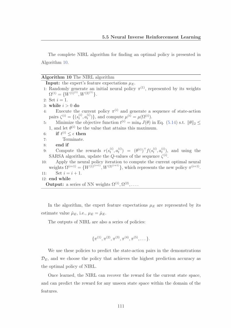
5.5 Neural Inverse Reinforcement Learning
The complete NIRL algorithm for finding an optimal policy is presented in
Algorithm 10.
Algorithm 10 The NIRL algorithmInput: the expert’s feature expectations μE.
1: Randomly generate an initial neural policy π(1), represented by its weightsΩ(1) = {W (1)(1) ,W (2)(1)}.
2: Set i = 1.3: while i > 0 do4: Execute the current policy π(i) and generate a sequence of state-action
pairs ζ(i) = {(s(i)t , a(i)t )}, and compute μ(i) = μ(Ω(i)).
5: Minimize the objective function t(i) = minθ J(θ) in Eq. (5.14) s.t. ‖θ‖2 ≤1, and let θ(i) be the value that attains this maximum.
6: if t(i) ≤ ε then7: Terminate.8: end if9: Compute the rewards r(s
(i)t , a
(i)t ) = (θ(i))�f(s(i)t , a
(i)t ), and using the
SARSA algorithm, update the Q-values of the sequence ζ(i).10: Apply the neural policy iteration to compute the current optimal neural
weights Ω(i+1) = {W (1)(i+1),W (2)(i+1)}, which represents the new policy π(i+1).
11: Set i = i+ 1.12: end while
Output: a series of NN weights Ω(1),Ω(2), . . . .
In the algorithm, the expert feature expectations μE are represented by its
estimate value μE, i.e., μE = μE.
The outputs of NIRL are also a series of policies:
{π(1), π(2), π(3), π(4), π(5), . . . }.
We use these policies to predict the state-action pairs in the demonstrations
DE, and we choose the policy that achieves the highest prediction accuracy as
the optimal policy of NIRL.
Once learned, the NIRL can recover the reward for the current state space,
and can predict the reward for any unseen state space within the domain of the
features.
111

5. LEARNING REWARD FUNCTIONS WITH NONLINEARNEURAL POLICY REPRESENTATIONS
5.5.5 Expert Demonstrations
Two types of demonstrations are used in this paper. The first one is the humanexpert demonstrations. A human expert choose the best policy but may stillnot an optimal one. The second one is the computer expert demonstrations. Acomputer expert can always give optimal policies, and therefore a modified A*algorithm is applied to generate optimal policies. Another advantage of computerexpert is that in some hazardous situations, human demonstrations cannot beavailable for the robot, so learning from computer experts bring less harm.
All the demonstration examples can be gathered either by the modified A*algorithm, or by the human expert, and NIRL algorithm learns the reward func-tion. Finally a MDP solver finds a policy mapping from input of world states tooutput of robot actions.
5.5.5.1 Computer-based Expert Demonstrations
The computer-based expert demonstrations are realized by the modified A* al-gorithm and we have presented it in Chapter 3.5.
The expert’s policy πE corresponds to the optimal deterministic policy.
5.5.5.2 Human Demonstrations
A human expert can also demonstrate their navigating strategy by themselves.An expert can control the learning robot by teleoperation or directly show therobot how to navigate. We model the human demonstration in Figure 5.3. Thehuman expert first gave some key points in the navigating map, and a smooth tra-jectory (Figure 5.3(a)) passing the key points is generated through interpolationtechniques. The trajectory is regarded as the planned path for the robot. Thenthe robot follows the path to collect state-action pairs (Figure 5.3(b)). Obviously,a human expert may not always deliver an optimal policy.
5.6 Experimental results
The mobile robot (see Chapter 2.5) is represented by a rectangle-shaped robot.It is equipped with 9 sensors to observe the surrounding environment, as shownin Figure 2.6. The environment map has a size of 100 m × 100 m. The obstacles
112

5.6 Experimental results
0 10 20 30 40 50 60 70 80 90 1000
10
20
30
40
50
60
70
80
90
100Expert Demo: 5
(a) A trajectory given by a human ex-pert
0 10 20 30 40 50 60 70 80 90 1000
10
20
30
40
50
60
70
80
90
100Expert Demo: 5
(b) Path following to collect data
Figure 5.3: A human expert demonstration.
are randomly scattered in the environment and the robot has no prior knowledge
of their numbers, sizes and positions. The initial position of the robot is placed at
(10, 10) and the target position, a red circle in the map, is found at (90, 90). The
velocity of the robot is fixed at 2 m/s. The mission of the robot is to start from
the initial position and to find an optimal path to arrive at the target position
without any collision with any obstacles. If no obstacles are detected, the robot
is designed to move towards the target.
The neural network adopted in the experiments has three layers: 16 in the
input layer, 8 in the hidden layer and 6 in the output layer. The inputs and
outputs are presented above in Section 5.4.1. Some experiment parameters are
selected as follows:
- Boundary distance: dbou = 10 m,
- Warning distance: dwarn = 5 m,
- Learning rate of Q function: α = 0.8,
- Learning rate of BPNN: σ = 0.4,
- Discount factor: γ = 0.65,
113

5. LEARNING REWARD FUNCTIONS WITH NONLINEARNEURAL POLICY REPRESENTATIONS
5.6.1 Comparison of Two Types of Demonstrations
In order to show the relationship between number of demonstrations and collected
samples, different numbers of demonstrations were tested: 20, 25, 30, 35, 40 and
50. Recall that one sample is one state-action pair. Each number is conducted 10
times. The average results are shown in Figure 5.4(a). Averagely, one trajectory
could contain 52-55 samples.
20 25 30 35 40 45 50800
1200
1600
2000
2400
2800
Number of trajectories
Am
ount
of c
olle
cted
sam
ples
human expertcomputer expert
(a) The average amount of collected samples in different num-bers of trajectories.
20 25 30 35 40 45 50
400
500
600
700
800
900
Number of trajectories
Am
ount
of n
onre
peat
ed v
isite
d st
ates
human expertcomputer expert
(b) The average amount of nonrepeated visited states in dif-ferent numbers of trajectories.
Figure 5.4: Expert demonstrations in different numbers of trajectories.
114

5.6 Experimental results
The human’s policies πE correspond to the sub-optimal stochastic policies.Due to the stochasticity, in the same states, there may exist many action pos-sibilities. We concern how many different states have been visited during thedemonstrations, therefore, we gave out the relation between the amount of non-repeated visited states and the number of demonstrations, as shown in Figure5.4(b).
Averagely, one trajectory could contain 13-19 nonrepeated visited states.
When robot follows the expert trajectories, the actions that the robot takemay be stochastic, that is, a suggested action may lead to a different actionaccording a probability P (a | a), see Figure 5.5.
0 10 20 30 40 50 60 70 80 90 1000
10
20
30
40
50
60
70
80
90
100Computer−based Expert Demo: No. 3
(a) An expert trajectory with severalstochastic actions
0 10 20 30 40 50 60 70 80 90 1000
10
20
30
40
50
60
70
80
90
100Computer−based Expert Demo: No. 17
(b) An expert trajectory with littlestochastic actions
Figure 5.5: Expert demonstrations with stochastic actions.
In Figure 5.5(a), we can see a number of stochastic actions, while in Figure5.5(b), there exists only one stochastic action.
5.6.2 Neural Inverse Reinforcement Learning
In this paper, 30 demonstrations are generated by modified A* algorithm. All ofthem have different configurations of random obstacle positions. The advantageof different maps is that the robot can always face new challenge and help gathermore state-action combination. Some of the human expert demonstrations arepresented in Figure 5.6.
115

5. LEARNING REWARD FUNCTIONS WITH NONLINEARNEURAL POLICY REPRESENTATIONS
0 10 20 30 40 50 60 70 80 90 1000
10
20
30
40
50
60
70
80
90
100Human Expert Demo: 1
Demo accomplished!Samples collected: 49 pairs.
0 10 20 30 40 50 60 70 80 90 1000
10
20
30
40
50
60
70
80
90
100Human Expert Demo: 7
Demo accomplished!Samples collected: 47 pairs.
Figure 5.6: Human expert demonstrations.
It is observed that the computer-based demonstrations can always provideoptimal paths, and this will greatly improve the robot learning performance com-pared to human teachers who cannot guarantee the quality of their demonstra-tions.
In each iteration of NIRL, an episode of 10 trajectories is generated using thecurrent policy and all the sequences of state-action pairs are collected that areused for updating the policy. In each trajectory, the robot tries to navigate indifferent environments in order to assure the diversity of state-action pairs. Anew episode will be started in the following three situations:
• The robot finds a collision free path to the target;
• The robot collides with an obstacle or the map borders;
• The robot runs out the moving steps.
The max-margin method is applied to learn the reward function by minimizingthe margin function J(θ) in Equation 5.14.
Figure 5.7 showed the change of the margin in MMP during the learningepisodes. We can tell the margin was stably diminishing towards 3. Hence, themargin between a learned policy was gradually approaching the expert policy,and this is exactly the learning objective.
116

5.6 Experimental results
0 20 40 60 80 100 120 1402
4
6
8
10
12
14
16
18
20
22
episodes
mar
gin
Figure 5.7: Changes of margin during the learning episodes.
0 20 40 60 80 100 120 1403.22
3.24
3.26
3.28
3.3
3.32
3.34
3.36
3.38
episodes
cost
Figure 5.8: Changes of NN cost during the learning episodes.
The nonlinear neural policy is trained for the state-action pairs collected underthe current policy. The goal is to minimize the cost J(Ω) in Equation (5.15) byiteratively updating the weights W (1) and W (2). The result is shown in Figure5.8.
In the first 20 episodes, the cost decreases fast and then becomes smaller
117

5. LEARNING REWARD FUNCTIONS WITH NONLINEARNEURAL POLICY REPRESENTATIONS
stably. Finally after 140 episodes, the cost converges and stays around 3.23.Once the training terminates, W (1) and W (2) stop updating and the learningprocess from demonstration is accomplished. It is now the time to examine therobot learning achievement.
5.6.3 Robot navigation in new unknown environments
In the navigation process, the weights W (1) and W (2) have converged to theiroptimal values. The mobile robot has learned how to behave in front of obstaclesin unexpected environments. Some of the navigation results are shown in Figure5.9.
It is observed that the paths that the robot chose may not be the optimalones due to a lack of complete knowledge of environment map, but they are stillfully acceptable and perfect enough to meet our expectation, especially in suchcomplicated and unstructured environments.
A successful navigation is one in which the robot succeeds in arriving at thetarget position. We tried 100 times of autonomous navigation by using variousnumber of expert demonstrations. We compare the rate of success with bothcomputer expert demonstrations (CE) and human expert demonstrations (HE).
Number of demos 25 30 40 50Rate of success of CE (%) 90 91 89 87Rate of success of HE (%) 82 85 84 84
Table 5.1: Rate of success in different numbers of demos
We observe that both types of demonstrations have proved to be reliable in-structors to the robot, and the computer expert did slightly better. Also moredemonstrations may not achieve a higher rate of success, because more demon-strations bring more stochastic in expressing the policies.
In order to test the robustness of the proposed algorithm, we gave the robot sixcompletely new navigation missions using the same weights with three differentrobot velocities, namely 1 m/s, 2 m/s and 3 m/s. 50 runs were conducted foreach velocities. The results are shown in Figure 5.10.
With the increase of obstacles presented in the surrounding environment, therobot becomes harder to navigate successfully. It is a normal situation that a
118

5.6 Experimental results
0 10 20 30 40 50 60 70 80 90 1000
10
20
30
40
50
60
70
80
90
100Robot Navigation
0 10 20 30 40 50 60 70 80 90 1000
10
20
30
40
50
60
70
80
90
100Robot Navigation
0 10 20 30 40 50 60 70 80 90 1000
10
20
30
40
50
60
70
80
90
100Robot Navigation
0 10 20 30 40 50 60 70 80 90 1000
10
20
30
40
50
60
70
80
90
100Robot Navigation
0 10 20 30 40 50 60 70 80 90 1000
10
20
30
40
50
60
70
80
90
100Robot Navigation
0 10 20 30 40 50 60 70 80 90 1000
10
20
30
40
50
60
70
80
90
100Robot Navigation
Figure 5.9: Robot navigation results in different environments.
bigger speed represents a need for quicker and more accurate reaction to the
environment changes, especially in an completely unknown environment. Despite
that, we can see that at least the robot could manage half of the navigation tasks
119

5. LEARNING REWARD FUNCTIONS WITH NONLINEARNEURAL POLICY REPRESENTATIONS
10 15 20 25 3020
25
30
35
40
45
50
No. obstacles
No.
suc
cess
ful n
avig
atio
ns
v=1m/sv=2m/sv=3m/s
Figure 5.10: Comparison of numbers of successful navigations in the environmentsof different numbers of obstacles.
and in most cases, the robot did pretty good. Therefore, the above experimentshave proven the feasibility and the stability of the proposed NIRL algorithm indifferent navigation environments and in different robot velocities.
5.6.4 Analysis of the weight changes
We analyzed the changes of neural policy weights W (1) and W (2) during thelearning process using NIRL. The change in one episode is the difference betweenthe weights before the learning and the ones after learning, i.e., ‖W (l)
new −W (l)‖1.The results are shown in Figure 5.11(a) and Figure 5.11(b). The X-axis representsthe number of episode and the Y-axis is the weight change.
The changes of the weight W (1) fluctuated strong in the beginning episodesand then went quiet around 0 after 20 episodes. The overall trend of weightchanges showed that the weight W (1) was turning stable as the learning processcarried on and W (1) converged to its optimal value.
In the meantime, the changes of weight W (2) fluctuated more fiercely throughall the learning process even though the changes went small after 60 episodes.That is because W (2) is directly related to the errors between the real outputsand the expected values in the neural network. Since the expected values are
120

5.6 Experimental results
0 20 40 60 80 100 120 140−0.1
0
0.1
0.2
0.3
0.4
0.5
chan
ge
episodes
(a) Changes of W (1) in learning process.
0 20 40 60 80 100 120 140
−0.25
−0.2
−0.15
−0.1
−0.05
0
0.05
0.1
0.15
0.2
0.25
episodes
chan
ge
(b) Changes of W (2) in learning process.
Figure 5.11: Changes of neural policy weights during the learning process.
calculated in Equation (5.16), and in each learning episode, the robot needs to
deal with a different environment, there are always errors between the real outputs
and the expected values. Therefore, it is reasonable that the weight W (2) is more
121

5. LEARNING REWARD FUNCTIONS WITH NONLINEARNEURAL POLICY REPRESENTATIONS
difficult to converge to an optimal value. However, the overall trend still toldus that W (2) was converging during the learning process, and the experimentsshowed that it did not affect the robot learning performance.
The changes of weights showed that NIRL converged to the optimal valuesafter approximately 80 learning episodes, and the learned policy is close enoughto the expert policy.
5.6.5 Autonomous Navigation in Dynamic Environments
Figure 5.12: Autonomous robot navigation in a dynamic environment usingNIRL.
122

5.6 Experimental results
We tested the NIRL algorithm in dynamic environments. The results are
shown in Figure 5.12. In the environment, the black solid objects are static
obstacles, and the purple rectangle ones are moving obstacles, whose moving
directions are unpredictable.
There are 10 static obstacles and 10 moving obstacles. When the robot de-
tected no obstacles around, it headed to the destination. From the experiment,
we can see that at time 13, the robot met a static obstacle on its left and a moving
obstacle in front of it, and the robot successfully avoided them and finally arrived
at the destination.
Therefore, NIRL has proven its feasibility in the application of autonomous
navigation in dynamic environments.
5.6.6 Discussions
We compare the NIRL algorithm with three major existing methods. The first one
is the apprenticeship learning (AL) in (Abbeel & Ng, 2004; Abbeel et al., 2008),
the baseline of the family of inverse reinforcement learning. The second one is
the relative entropy inverse reinforcement learning (RE), proposed in (Boularias
et al., 2011), a popular IRL algorithm using the theory of entropy. The last one
is the structured classification inverse reinforcement learning (SCIRL), presented
in (Klein et al., 2012a), a recent work using max-margin method for a batch
model-free learning algorithm.
We fixed the robot velocity at 2 m/s at the number of obstacles was 20. We
conducted 25 runs for each learning method and each run was tested on 100 times
of autonomous navigation.
For all the methods, we implemented the same computer expert. The com-
parison of the rate of success are shown in Table 5.2.
NIRL AL RE SCIRLAverage rate (%) 83 66 78 79
Best rate (%) 94 82 87 88Worst rate (%) 69 43 61 60
Table 5.2: Comparison of the rate of success versus different IRL methods.
123

5. LEARNING REWARD FUNCTIONS WITH NONLINEARNEURAL POLICY REPRESENTATIONS
From the results, we can see that NIRL achieved the best rate of success. REand SCIRL performed almost equally and slight worse than our NIRL algorithm.AL, as a pioneer algorithm, did the worst.
Therefore, the NIRL algorithm had a better performance in autonomous nav-igation tasks over the other three methods.
5.7 Conclusion
In the previous chapters, we have investigated two types of robot learning meth-ods. The first one is to learn a policy from expert demonstrations, and the secondone is to learn by itself by interacting with the surrounding unknown environ-ments without any expert indication.
This chapter presents a third robot learning method, that the robot tries tounderstand a expert behaviors in executing one specific task by means of learningthe underlying rewards from the expert demonstrations. This method is underthe framework of inverse reinforcement learning. We developed our method, theneural inverse reinforcement learning algorithm. We first proposed a nonlinearneural policy representation by incorporating an artificial neural network. Thisexplicit policy representation make the learning algorithm easy to implement.NIRL is also a method that does not assume the expert to be optimal. Weproposed to applied maximum a posteriori to pretreat the suboptimal samplesand later use the refined samples to NIRL. Then we adopted the maximum marginmethod to learn the reward through minimizing the maximum margin betweenthe expert policy and the learned policy. Finally, we update the nonlinear neuralpolicy using the learned reward function.
The experiment results show the feasibility and the robustness of the proposedNIRL algorithm, and he robot can complete autonomous navigation tasks safelyin an unpredicted dynamic environment. The robot not only can imitate whatthe expert behave but also understand why the expert behave that way throughlearning the reward function. An autonomous mobile robot equipped with suchlearning ability is what we desire during the whole dissertation.
124

Conclusions and Perspectives
In this chapter, we will conclude the dissertation by summarizing the main resultsand then present some perspectives of future research to complete and improvethis work.
Conclusions
Mobile robots are now playing a significant role in our society, the capability ofautonomous navigation in dynamic environments is one of the fundamental skills.The requirement that the robot should be able to react to changes in environ-mental conditions led to the production of robust and reliable controllers that candeal with the uncertainty of the world. Since it is unlikely that we can foreseeall potential real-world situations sufficiently accurate, a pre-programmed robotcannot meet the future requirements, especially when interaction with human isneeded. The aim of this dissertation has been focused on empowering a mobilerobots with an intelligent learning and adaptive ability that can cater to changingenvironments.
In this dissertation, we proposed three robot learning frameworks within dif-ferent situations.
• Efficient policy learning from expert demonstrations. (Chapter 3)
Human-beings are born with imitation ability, so should robots. When anexpert demonstrates one specific task to robots, robots should know to imi-tate or learn how to behave or how to make decisions as their teacher does.Here comes our method of efficient policy learning from expert demonstra-tions. Different from previous work on learning from demonstration, weplaced our focus on human experts are not available to robots. Instead,an improved version of A* is designed to stimulate expert examples. We
125

CONCLUSIONS AND PERSPECTIVES
established a decision-making process and represented the policy by usingneural network. This algorithm can be efficiently applied to autonomousnavigation tasks. (Xia et al., 2015)
• Self-learning in autonomous navigation using neural network based Q-learning.(Chapter 4)
An intelligent robot should also learn to make decisions even without anydemonstrations. That is realized by interacting with the environment oftasks. Based on these assumptions, we proposed neural network basedQ-learning. Since we have proved that a neural network could be an ap-propriate policy representation, we improved the Q-learning algorithm byincorporating this representation. Results showed that our method greatlyimproved the learning performance and increase the convergence speed.(Xia & El Kamel, 2014a,b,c, 2015d)
• Learning reward from multiple examples via neural inverse reinforcementlearning. (Chapter 5)
Experts may not always demonstrate optimal policies. In these cases, in-verse reinforcement learning provides a way to learn reward correspondingto each state. However, the generalization of undemonstrated states affectsthe performance of algorithm. We proposed the neural inverse reinforce-ment learning, which aligned our interest in neural network. Our methodimproved the performance on learning a reward function. This algorithmcould be successfully applied to autonomous navigation, and as well as otherapplications. (Xia & El Kamel, 2015a,b)
All the above robot learning methods are model-free algorithms that are moresuitable in real applications since a model of an unknown world is impossible toacquire.
Future Work
First of all, this dissertation has provided theoretical foundations on mobile robotlearning and achieved reliable results in simulators. Tests on real vehicles inoutdoor environments could be conducted in order to carry the robot learning astep forward.
126

CONCLUSIONS AND PERSPECTIVES
Second, an intelligent robot control system relies on the various sensors thatcapture the environmental information. With the development of robot sensors,an robot should be able to learn a control strategy from the rich variety of sensorydata, especially those of visual and audio inputs. The ability of learning froma complexity of sensor data will not only endow the robot intelligence but alsoenhance the robot interaction with humans.
Third, robot learning should also be developed in multi-robot systems. Moreand more labor work would be done by a group of robots, and thus it would benecessary to pursue robot learning techniques to predict the behavior and betterinteract with other robots.
Last but not least, the deep reinforcement learning method has been presentedby applying covolutional neural network (CNN) (Mnih et al., 2013). As part ofdeep learning family, CNN has shown its power in image recognition and computervision, therefore, researches in deep reinforcement learning will surely bring newbreakouts to robotics.
127

CONCLUSIONS AND PERSPECTIVES
128
Résumé Étendu en Français
Introduction
Les robots modernes sont conçus pour aider ou remplacer les humains à effectuerdes opérations complexes, des planifications, ou des contrôles de tâches. Les exem-ples contiennent la manipulation d’objets, l’assistance d’experts dans une variétéde professions, la navigation dans des environnements extérieurs, l’explorationdes territoires inconnus, et la conduite dans les zones urbaines. Il est générale-ment un processus compliqué pour la conception d’un schéma de contrôle pources robots afin d’exécuter ces tâches, même pour les personnes spécialisées dansla programmation de robots. Elles doivent prendre en compte délibérément lesspécifications de toutes les situations que le robot peut rencontrer et elle nécessi-tent à la création nouveau et différent à la main pour chaque tâche particulière.Ce genre de pré-programmation manuelle est généralement un travail intense etennuyeux. Plutôt que de pré-programmer un robot pour toutes les tâches, il seraitplus utile si le robot pourrait apprendre ces tâches par eux-mêmes.
Movitation de la Recherche
La capacité de navigation autonome joue un rôle important dans la des voîturesautonomes sans conducteur de l’état de l’art. Remontée en 2003, La DefenseAdvanced Research Projects Agency (DARPA) du département de la Défensedes États-Unis a organisé le “Grand Challenge” pour stimuler le développementdes technologies nécessaires pour créer les véhicules terrestres sans pilote et au-tonomes capables de parcourir un cours substantielle hors route dans une périodelimitée. Le défi nécessite pour les véhicules de naviguer dans un circuit de 142
129

RÉSUMÉ ÉTENDU EN FRANÇAIS
miles à travers du désert de Mojaves en ne pas surpassant 10 h. La premièrecompétition a eu lieu le 13 mars, 2004. 15 véhicules ont y participé, mais mal-heureusement, aucune n’ont pu terminé plus de 5% de l’ensemble du cours. Parconséquent, le relancement d’un deuxième événement “DARPA Grand Challenge”était prévue le 8 octobre 2005. Cinq des 23 véhicules ont conquis le cours avecsuccès, et "Stanley" de Stanford (voir Figure 1) a été couronné le champion avecun résultat de 6 h 53 min. Cette voiture robotisée était une étape importantedans la quête des voitures autonomes modernes.
Figure 1: Stanley: le champion du DARPA Grand Challenge 2005. (Thrun et al.,2006)
Deux ans plus tard, le “DARPA Urban Challenge” a eu lieu le 3 novembre,2007, et a appelé à des véhicules autonomes de conduire 97 km à travers unemaquette d’environnement urbaine en moins de 6 heures, en interagissant avecdes obstacles et des autres véhicules en mouvement et aussi en respectant tous lesrèglements de la circulation. La véhicule “Boss” a été déclaré la gagnante (Urmsonet al., 2008) et “Junior” (Montemerlo et al., 2008) a remporté la deuxième place.Ces vésicules ont également été considérées comme le premier prototype de lavoiture sans conducteur de Google.
Traditionnellement, un programmeur humain utilisait son propre compréhen-sion sur les tâches désirées et dressait un plan à l’avance pour coder un contrôleurde robot qui permettait de répondre à toutes les situations où le robot pouvaitfaire face. Si des erreurs ou de nouvelles circonstances apparaissaient, le robotdevait être programmé à nouveau.
130

RÉSUMÉ ÉTENDU EN FRANÇAIS
Motivé par les défis du DARPA et les voîtures sans conducteur de Google,
cette thèse se concentre sur doter les robots la capacité d’apprendre de nouvelles
techniques et d’améliorer leur compétences autonomes. Par ce moyen, les robots
peuvent prendre de décisions intelligentes et adapter à des incertitudes et des
changements imprévus dans les environnements stochastiques et dynamiques.
Cette thèse étudie le pilotage intelligent de robots dans les tâches de naviga-
tions autonomes et examiner l’apprentissage des robots dans trois aspects.
Apprentissage efficace d’une politique par démon-strations d’experts
Dans le premier aspect, nous considérons l’apprentissage des robots par dé-
monstrations d’experts. Cette méthode est inspirée par l’instinct humain de
l’imitation. Les humains sont nées avec la capacité d’imitation, et les robots
doivent donc aussi posséder cette capacité.
Nous fournissons un robot des exemples d’une tâche faite par un expert, le
robot observe ces exemple et apprend une politique efficace à partir de ces données
et de généraliser sur toutes les situations potentielles qui ne sont pas données dans
les exemples. Dans la navigation autonome, une série de trajectoires sont données
au robot, le robot apprend à construire une stratégie de contrôle afin d’accomplir
la navigation autonome dans un environnent inconnu et dynamique (voir Figure
2).
���
"���������,����-���� ��%�����.
)����������
/�����������
��������%���%��#
Figure 2: Un schéma simple de l’apprentissage d’une politique.
131

RÉSUMÉ ÉTENDU EN FRANÇAIS
Nous avons intégré un mécanisme d’inférence en appliquant un réseau deneurones. Après avoir obtenu les démonstrations d’un expert, le robot sélectionneune base de données valables, et cette base est envoyée vers le réseau de neuronespour s’entraîner. L’algorithme de rétropropagation du gradient est appliqué pourminimiser itérativement une fonction d’entropie croisée. Notre méthode montreque avec un nombre acceptable de démonstrations, la structure d’apprentissagepeut converger vers une politique optimale dans un nombre d’épisodes pas grand,et aussi le robot peut acquérir les compétences de navigation indépendants dansun nouveau environnent dynamique.
En plus, nous proposons un expert informatique basé sur une variante del’algorithme A*. Cet expert peut offrir des trajectoires dans les cas extrêmes oùles démonstrations humaines sont indisponibles.
L’avantage de cette méthode d’apprentissage efficace d’une politique est que ledesigner n’ont pas besoin de pré-programmer un robot précisément. L’utilisateurspeuvent facilement demander les robots d’exécuter un comportement par leurdémontrer comment le faire.
Apprentissage par renforcement sous des politiquesstochastiques
Dans le deuxième aspect, nous considérons l’apprentissage de robots sans dé-monstrations d’experts et l’application dans la navigation autonome. C’est pourtraiter les situations où les humains ont très peu d’expérience préalable, et doncaucunes démonstrations seraient être fourni. Un robot intelligent doit aussi pos-séder la compétence d’apprendre par soi-même à prendre des décisions sans au-cune direction.
Nous proposons une méthode d’apprentissage en ligne via d’expérience accu-mulée qui est basée sur l’apprentissage par renforcement (voir Figure 3). Elleest réalisée par les interactions exploratoires entre le robot et son environnement.L’algorithme de Q-learning est une méthode qui ne nécessite aucun modèle ini-tial du système, et Q-learning peut être appliqué pour trouver une suite d’actionsassociées à des états d’un Processus de décision markovien. Nous utilisons Q-learning pour mettre à jour les Q-valeurs dans chaque étape de temps. Différenteque les autres méthodes concernant Q-learning qui utilisent les exemples venants
132

RÉSUMÉ ÉTENDU EN FRANÇAIS
d’une seule interaction, notre méthode accumule les exemples venant de toutes
les interactions dans une base de donnée, ainsi que leurs Q-valeurs renouvelées.
La base est utilisée par un réseau de neurones afin de optimiser itérativement
une politique de contrôle en temps réel. Pendant le processus d’interaction, le
robot doit balancer l’exploration et l’exploitation, donc son politique est traitée
stochastique.
���
)�������-���� � %��0�����
/����������,����-���
� ��%����.
���% �������,����-�12%������
3��%���������
4����%��%��#
"����������,��
Figure 3: Un schéma simple de l’apprentissage en ligne via d’expérience accu-mulée.
Cette méthode évite l’inconvénient de celles dans la littérature qui abandon-
nent la plupart de données collectées pendant le processus d’interaction. Aussi,
comme cette méthode améliore la politique en temps réel, sa performance est plus
stable que celle de l’apprentissage en batch. Les expériences montrent le succès
d’appliquer notre méthode à la navigation autonome et dépense moins de temps
pour trouver une politique optimale.
133

RÉSUMÉ ÉTENDU EN FRANÇAIS
Apprentissage de la fonction de récompense via unereprésentation non-linéaire de la politique neuronale
Dans le troisième aspect, nous considérons que le robot apprend à compren-dre les comportements d’un expert qui fait des démonstrations. Il est réalisépar apprendre les récompenses potentielles dans les états via l’apprentissage parrenforcement inverse. C’est parce que une fonction de récompense n’est pas nor-malement facile à préciser et imiter directement un expert poserait le problèmede l’imprécision si l’expert acte de manière non-optimale. Par conséquent, étantdonné les démonstrations, les robots ne doivent pas seulement apprendre à as-socier les états et les actions, mais aussi essayer de comprendre les récompenses.
Nous proposons une méthode, l’apprentissage neuronale par renforcement in-verse (voir Figure 4).
���4����%�5�� ������%�)���������� ��������%�
��%��#
����%�-����
�--�������
����- �����
6��%����� ��%���%��#����������
3��%���������
�����#��
Figure 4: Un schéma simple de l’apprentissage de la fonction de récompense.
Une représentation non-linéaire de la politique neuronale est tout d’aborddéveloppée afin d’établir une connexion explicite entre les états et les actions,et un réseau de neurones est également intégré pour généraliser les actions surles états non visités parmi les démonstrations. Ensuite la méthode proposéede l’apprentissage neuronale par renforcement inverse est appliquée à appren-dre la fonction de récompense. Après avoir obtenu cette fonction, nous pouvonsd’avantage optimiser itérativement la politique neuronale via les interactions pro-gressives entre le robot et l’environnement et finalement déduire une politiqueoptimale. Afin de traiter les démonstrations non-optimales, un raffinement estdésigné à pré-procéder les démonstrations en profitant du maximum a posteriori.
134

RÉSUMÉ ÉTENDU EN FRANÇAIS
Les résultats expérimentaux ont montré une performance fiable et la ro-bustesse dans la tâche de navigation autonome en utilisant notre méthode pro-posée.
Conclusions et Perspectives
Cette thèse contribue à la conception de commande intelligente afin de réaliserl’apprentissage des robots mobiles durant la navigation autonome. Les résultatsexpérimentaux ont confirmé l’efficacité et la robustesse de toutes les méthodesque nous avons proposé, et en plus, l’application de ces méthodes peut largementsoulager du travail fastidieux de préprogrammer un robot manuellement.
Contributions
L’objectif de cette thèse est centrée sur l’habilitation pour les robots mobiles descapacités d’apprentissage intelligent et d’adaptation qui permet de répondre àdes environnements changeants. Les contributions sont développées dans troisdomaines:
1. Dans les situations où les démonstrations optimales sont fournies, nousavons proposé la méthode d’apprentissage efficace d’une politique par dé-monstrations d’experts (Chapître 3). Cette méthode produit une perfor-mance stable et agréable avec un nombre acceptable de démonstrations. Elleéconomise aussi beaucoup de temps pendant le processus d’apprentissage.
2. Dans les situations où les humains manquent d’experience préalable, nousavons proposé la méthode d’apprentissage en ligne via d’expérience accu-mulée (Chapître 4). Cette méthode permet d’apprendre par soi-même unestratégie de contrôle et de traiter l’environnement progressivement en uncertain nombre d’épisodes inférieur a la littérature. Notre méthode réussitune performance fiable et stable.
3. Dans les situations où les démonstrations fournies ne sont pas toujours op-timales, nous avons proposé la méthode d’apprentissage neuronale par ren-forcement inverse (Chapître 5). Cette méthode peut efficacement apprendrela fonction de récompense en dessous de toute l’espace d’états. Cela permet
135

RÉSUMÉ ÉTENDU EN FRANÇAIS
de mieux comprendre les comportements d’experts et ensuite calculer unepolitique de contrôle optimale, même si les exemples sont non-optimaux.
Perspectives
Tout d’abord, cette thèse a fourni les théories fondementales sur l’apprentissagede robots mobiles et a obtenu des résultats fiables dans les simulateurs. Tests survéhicules réelles dans des environnements extérieurs pourraient être menées afinde réaliser l’apprentissage de robots un pas en avant. En plus, d’autre applicationspourraient aussi être étudié.
Deuxièmement, un système de contrôle du robot intelligent repose sur les dif-férents capteurs qui perçoivent l’environnement. Avec le développement de cap-teurs, un robot doit être capable d’apprendre une stratégie de pilotage à partirde la variété riche de données sensorielles, en particulier celle des entrées au-dio et visuelles. La capacité d’apprendre à partir d’une complexité des donnéesde capteurs non seulement dotera l’intelligence du robot, mais aussi améliorerl’interaction de robot avec les humains.
Troisièmement, l’apprentissage de robot devrait également être développédans les systèmes de multi-robots. Puisque de plus en plus de travaux seraienteffectués par un groupe de robots, il serait donc nécessaire de poursuivre les tech-niques d’apprentissage de robot pour prédire les comportements d’autre robotsen coopération et mieux interagir avec eux.
Dernièrement, la méthode de l’apprentissage profond par renforcement a étéprésenté par l’application du réseau neuronal covolutional (CNN, convolutionalneural network en anglais) (Mnih et al., 2013). Dans le cadre de la famille del’apprentissage profond, CNN a montré sa puissance en reconnaissance d’imageet de vision par ordinateur, par conséquent, des recherches en l’apprentissageprofond par renforcement apporteront certainement de nouveaux avancements àla robotique.
136

Bibliography
Abbeel, P. & Ng, A.Y. (2004). Apprenticeship learning via inverse reinforce-ment learning. In Proceedings of the twenty-first international conference onMachine learning , 1, ACM.
Abbeel, P. & Ng, A.Y. (2005). Exploration and apprenticeship learning inreinforcement learning. In Proceedings of the 22nd international conference onMachine learning , 1–8, ACM.
Abbeel, P., Coates, A., Quigley, M. & Ng, A.Y. (2007). An applicationof reinforcement learning to aerobatic helicopter flight. Advances in neural in-formation processing systems, 19, 1.
Abbeel, P., Dolgov, D., Ng, A.Y. & Thrun, S. (2008). Apprenticeshiplearning for motion planning with application to parking lot navigation. InIntelligent Robots and Systems, 2008. IROS 2008. IEEE/RSJ InternationalConference on, 1083–1090, IEEE.
Abbeel, P., Coates, A. & Ng, A.Y. (2010). Autonomous helicopter aero-batics through apprenticeship learning. The International Journal of RoboticsResearch.
Alissandrakis, A., Nehaniv, C.L. & Dautenhahn, K. (2002). Imitationwith alice: Learning to imitate corresponding actions across dissimilar embod-iments. Systems, Man and Cybernetics, Part A: Systems and Humans, IEEETransactions on, 32, 482–496.
Andrieu, C., De Freitas, N., Doucet, A. & Jordan, M.I. (2003). Anintroduction to mcmc for machine learning. Machine learning , 50, 5–43.
137

BIBLIOGRAPHY
Argall, B.D., Chernova, S., Veloso, M. & Browning, B. (2009). A sur-vey of robot learning from demonstration. Robotics and autonomous systems,57, 469–483.
Atkeson, C.G. & Schaal, S. (1997). Robot learning from demonstration. InMachine Learning (ICML), International Conference on, vol. 97, 12–20.
Bagnell, J.A., Bradley, D., Silver, D., Sofman, B. & Stentz, A. (2010).Learning for autonomous navigation. Robotics & Automation Magazine, IEEE ,17, 74–84.
Bentivegna, D.C., Atkeson, C.G. & Cheng, G. (2004a). Learning fromobservation and practice using primitives. In AAAI 2004 Fall Symposium onReal-life Reinforcement Learning , Citeseer.
Bentivegna, D.C., Atkeson, C.G., UDE, A. & Cheng, G. (2004b). Learn-ing to act from observation and practice. International Journal of HumanoidRobotics , 1, 585–611.
Bertsekas, D.P. (1996). Dynamic programming and optimal control , vol. 1.Athena Scientific Belmont, Massachusetts.
Bertsekas, D.P. (1998). Network Optimization: continuous and discrete meth-ods , vol. 8. Athena Scientific.
Billard, A. & Grollman, D. (2013). Robot learning by demonstration. Schol-arpedia, 8, 3824.
Billard, A., Calinon, S., Dillmann, R. & Schaal, S. (2008). Robotprogramming by demonstration. In Springer handbook of robotics , 1371–1394,Springer.
Bohren, J., Foote, T., Keller, J., Kushleyev, A., Lee, D., Stewart,
A., Vernaza, P., Derenick, J., Spletzer, J. & Satterfield, B. (2008).Little ben: the ben franklin racing team’s entry in the 2007 darpa urban chal-lenge. Journal of Field Robotics , 25, 598–614.
Boularias, A. & Chaib-Draa, B. (2013). Apprenticeship learning with fewexamples. Neurocomputing , 104, 83–96.
138

BIBLIOGRAPHY
Boularias, A., Kober, J. & Peters, J.R. (2011). Relative entropy inversereinforcement learning. In International Conference on Artificial Intelligenceand Statistics, 182–189.
Boularias, A., Krömer, O. & Peters, J. (2012). Structured apprenticeshiplearning. In Machine Learning and Knowledge Discovery in Databases, 227–242, Springer.
Bradtke, S.J. & Barto, A.G. (1996). Linear least-squares algorithms fortemporal difference learning. Machine Learning , 22, 33–57.
Breazeal, C., Hoffman, G. & Lockerd, A. (2004). Teaching and workingwith robots as a collaboration. In Proceedings of the Third International JointConference on Autonomous Agents and Multiagent Systems-Volume 3 , 1030–1037, IEEE Computer Society.
Carreras, M., Yuh, J., Batlle, J. & Ridao, P. (2005). A behavior-based scheme using reinforcement learning for autonomous underwater vehicles.Oceanic Engineering, IEEE Journal of , 30, 416–427.
Chernova, S. & Veloso, M. (2007). Confidence-based policy learning fromdemonstration using gaussian mixture models. In Proceedings of the 6th inter-national joint conference on Autonomous agents and multiagent systems, 233,ACM.
Choi, J. & Kim, K.E. (2011a). Inverse reinforcement learning in partially ob-servable environments. The Journal of Machine Learning Research, 12, 691–730.
Choi, J. & Kim, K.E. (2011b). Map inference for bayesian inverse reinforcementlearning. In Advances in Neural Information Processing Systems , 1989–1997.
Choi, J. & Kim, K.E. (2012). Nonparametric bayesian inverse reinforcementlearning for multiple reward functions. In Advances in Neural Information Pro-cessing Systems, 305–313.
Coates, A., Abbeel, P. & Ng, A.Y. (2008). Learning for control from multipledemonstrations. In Proceedings of the 25th international conference on Machinelearning , 144–151, ACM.
139

BIBLIOGRAPHY
Cobo, L.C., Subramanian, K., Isbell, C.L., Lanterman, A.D. &
Thomaz, A.L. (2014). Abstraction from demonstration for efficient reinforce-ment learning in high-dimensional domains. Artificial Intelligence, 216, 103–128.
Cummins, M. & Newman, P. (2007). Probabilistic appearance based naviga-tion and loop closing. In Robotics and automation, 2007 IEEE internationalconference on, 2042–2048, IEEE.
Dimitrakakis, C. & Rothkopf, C.A. (2012). Bayesian multitask inverse re-inforcement learning. In Recent Advances in Reinforcement Learning , 273–284,Springer.
Duan, Y., Liu, Q. & Xu, X. (2007). Application of reinforcement learning inrobot soccer. Engineering Applications of Artificial Intelligence, 20, 936–950.
El-Fakdi, A. & Carreras, M. (2013). Two-step gradient-based reinforcementlearning for underwater robotics behavior learning. Robotics and AutonomousSystems , 61, 271–282.
Ernst, D., Geurts, P. & Wehenkel, L. (2005). Tree-based batch modereinforcement learning. In Journal of Machine Learning Research, 503–556.
Fabiani, P., Fuertes, V., Piquereau, A., Mampey, R. & Teichteil-
Königsbuch, F. (2007). Autonomous flight and navigation of vtol uavs: fromautonomy demonstrations to out-of-sight flights. Aerospace Science and Tech-nology , 11, 183–193.
Fard, M.M. & Pineau, J. (2009). Mdps with non-deterministic policies. InAdvances in neural information processing systems , 1065–1072.
Gosavi, A. (2009). Reinforcement learning: A tutorial survey and recent ad-vances. INFORMS Journal on Computing , 21, 178–192.
Harmon, M.E. & Harmon, S.S. (1996). Reinforcement learning: A tutorial.WL/AAFC, WPAFB Ohio, 45433.
He, H., Eisner, J. & Daume, H. (2012). Imitation learning by coaching. InAdvances in Neural Information Processing Systems , 3149–3157.
140

BIBLIOGRAPHY
Helmick, D.M., Roumeliotis, S.I., Cheng, Y., Clouse, D.S., Ba-
jracharya, M. & Matthies, L.H. (2006). Slip-compensated path followingfor planetary exploration rovers. Advanced Robotics, 20, 1257–1280.
Hester, T., Quinlan, M. & Stone, P. (2012). Rtmba: A real-time model-based reinforcement learning architecture for robot control. In Robotics andAutomation (ICRA), 2012 IEEE International Conference on, 85–90, IEEE.
Huang, B.Q., Cao, G.Y. & Guo, M. (2005). Reinforcement learning neuralnetwork to the problem of autonomous mobile robot obstacle avoidance. InMachine Learning and Cybernetics, 2005. Proceedings of 2005 InternationalConference on, vol. 1, 85–89, IEEE.
Jain, A., Wojcik, B., Joachims, T. & Saxena, A. (2013). Learning trajec-tory preferences for manipulators via iterative improvement. In Advances inNeural Information Processing Systems , 575–583.
Jaradat, M.A.K., Al-Rousan, M. & Quadan, L. (2011). Reinforce-ment based mobile robot navigation in dynamic environment. Robotics andComputer-Integrated Manufacturing , 27, 135–149.
Kaelbling, L.P., Littman, M.L. & Moore, A.W. (1996). Reinforcementlearning: A survey. Journal of artificial intelligence research, 237–285.
Kaelbling, L.P., Littman, M.L. & Cassandra, A.R. (1998). Planning andacting in partially observable stochastic domains. Artificial intelligence, 101,99–134.
Klein, E., Geist, M. & Pietquin, O. (2012a). Batch, off-policy and model-free apprenticeship learning. In Recent Advances in Reinforcement Learning ,285–296, Springer.
Klein, E., Geist, M., Piot, B. & Pietquin, O. (2012b). Inverse reinforce-ment learning through structured classification. In Advances in Neural Infor-mation Processing Systems, 1007–1015.
Klein, É., Piot, B., Geist, M. & Pietquin, O. (2012c). Structured classifica-tion for inverse reinforcement learning. Journal of Machine Learning Research,2012, 1–14.
141

BIBLIOGRAPHY
Knudson, M. & Tumer, K. (2011). Adaptive navigation for autonomousrobots. Robotics and Autonomous Systems, 59, 410–420.
Kober, J. & Peters, J. (2010). Imitation and reinforcement learning. Robotics& Automation Magazine, IEEE , 17, 55–62.
Kober, J., Bagnell, J.A. & Peters, J. (2013). Reinforcement learn-ing in robotics: A survey. The International Journal of Robotics Research,0278364913495721.
Kolter, J.Z. & Ng, A.Y. (2009). Policy search via the signed derivative. InRobotics: science and systems.
Kormushev, P., Calinon, S. & Caldwell, D.G. (2010). Robot motor skillcoordination with em-based reinforcement learning. In Intelligent Robots andSystems (IROS), 2010 IEEE/RSJ International Conference on, 3232–3237,IEEE.
Kunz, C., Murphy, C., Camilli, R., Singh, H., Bailey, J., Eustice, R.,
Jakuba, M., Nakamura, K.I., Roman, C., Sato, T. et al. (2008). Deepsea underwater robotic exploration in the ice-covered arctic ocean with auvs.In Intelligent Robots and Systems, 2008. IROS 2008. IEEE/RSJ InternationalConference on, 3654–3660, IEEE.
Lagoudakis, M.G. & Parr, R. (2003). Least-squares policy iteration. TheJournal of Machine Learning Research, 4, 1107–1149.
Levine, S., Popovic, Z. & Koltun, V. (2010). Feature construction for inversereinforcement learning. In Advances in Neural Information Processing Systems ,1342–1350.
Levine, S., Popovic, Z. & Koltun, V. (2011). Nonlinear inverse reinforce-ment learning with gaussian processes. In Advances in Neural Information Pro-cessing Systems, 19–27.
Levine, S., Finn, C., Darrell, T. & Abbeel, P. (2015). End-to-end trainingof deep visuomotor policies. arXiv preprint arXiv:1504.00702 .
142

BIBLIOGRAPHY
Li, C., Zhang, J. & Li, Y. (2006). Application of artificial neural network basedon q-learning for mobile robot path planning. In Information Acquisition, 2006IEEE International Conference on, 978–982, IEEE.
Lockerd, A. & Breazeal, C. (2004). Tutelage and socially guided robotlearning. In Intelligent Robots and Systems, 2004.(IROS 2004). Proceedings.2004 IEEE/RSJ International Conference on, vol. 4, 3475–3480, IEEE.
Lopes, M., Melo, F. & Montesano, L. (2009). Active learning for rewardestimation in inverse reinforcement learning. In Machine Learning and Knowl-edge Discovery in Databases, 31–46, Springer.
Melo, F.S., Lopes, M. & Ferreira, R. (2010). Analysis of inverse reinforce-ment learning with perturbed demonstration. In ECAI , 349–354.
Michini, B. & How, J.P. (2012). Bayesian nonparametric inverse reinforcementlearning. In Machine Learning and Knowledge Discovery in Databases, 148–163, Springer.
Michini, B., Cutler, M. & How, J.P. (2013). Scalable reward learning fromdemonstration. In Robotics and Automation (ICRA), 2013 IEEE InternationalConference on, 303–308, IEEE.
Miljković, Z., Mitić, M., Lazarević, M. & Babić, B. (2013). Neural net-work reinforcement learning for visual control of robot manipulators. ExpertSystems with Applications, 40, 1721–1736.
Mitchell, T.M. (1997). Machine learning. 1997. Burr Ridge, IL: McGraw Hill ,45.
Mnih, V., Kavukcuoglu, K., Silver, D., Graves, A., Antonoglou, I.,
Wierstra, D. & Riedmiller, M. (2013). Playing atari with deep reinforce-ment learning. arXiv preprint arXiv:1312.5602 .
Moldovan, T.M. & Abbeel, P. (2012). Safe exploration in markov decisionprocesses. In Proceedings of the 29th International Conference on MachineLearning (ICML-12), 1711–1718.
143

BIBLIOGRAPHY
Montemerlo, M., Becker, J., Bhat, S., Dahlkamp, H., Dolgov, D.,
Ettinger, S., Haehnel, D., Hilden, T., Hoffmann, G., Huhnke, B.
et al. (2008). Junior: The stanford entry in the urban challenge. Journal offield Robotics , 25, 569–597.
Mori, T., Howard, M. & Vijayakumar, S. (2011). Model-free apprenticeshiplearning for transfer of human impedance behaviour. In Humanoid Robots (Hu-manoids), 2011 11th IEEE-RAS International Conference on, 239–246, IEEE.
Mülling, K., Kober, J., Kroemer, O. & Peters, J. (2013). Learning to se-lect and generalize striking movements in robot table tennis. The InternationalJournal of Robotics Research, 32, 263–279.
Navarro-Guerrero, N., Weber, C., Schroeter, P. & Wermter, S.
(2012). Real-world reinforcement learning for autonomous humanoid robotdocking. Robotics and Autonomous Systems, 60, 1400–1407.
Neu, G. & Szepesvári, C. (2007). Apprenticeship learning using inverse rein-forcement learning and gradient methods. In Proc. UAI .
Ng, A. (2011). Sparse autoencoder. CS294A Lecture notes, 72.
Ng, A.Y. (2006). Reinforcement learning and apprenticeship learning for roboticcontrol. In Algorithmic Learning Theory , 29–31, Springer.
Ng, A.Y. & Russell, S.J. (2000). Algorithms for inverse reinforcement learn-ing. In Machine Learning (ICML), International Conference on, 663–670.
Ng, A.Y., Harada, D. & Russell, S. (1999). Policy invariance under rewardtransformations: Theory and application to reward shaping. In ICML, vol. 99,278–287.
Ng, A.Y., Coates, A., Diel, M., Ganapathi, V., Schulte, J., Tse, B.,
Berger, E. & Liang, E. (2006). Autonomous inverted helicopter flight viareinforcement learning. In Experimental Robotics IX , 363–372, Springer.
Nicolescu, M.N. & Matarić, M.J. (2001). Learning and interacting inhuman-robot domains. Systems, Man and Cybernetics, Part A: Systems andHumans, IEEE Transactions on, 31, 419–430.
144

BIBLIOGRAPHY
Nicolescu, M.N. & Matarić, M.J. (2003). Natural methods for robot tasklearning: Instructive demonstrations, generalization and practice. In Proceed-ings of the second international joint conference on Autonomous agents andmultiagent systems, 241–248, ACM.
O’kane, J.M., Tovar, B., Cheng, P. & LaValle, S.M. (2005). Algorithmsfor planning under uncertainty in prediction and sensing. Autonomous MobileRobots: Sensing, Control, Decision-Making, and Applications, Series in Con-trol Engineering , 501–547.
Peters, J., Mülling, K. & Altun, Y. (2010). Relative entropy policy search.In AAAI .
Piot, B., Geist, M. & Pietquin, O. (2013). Learning from demonstrations:Is it worth estimating a reward function? In Machine Learning and KnowledgeDiscovery in Databases, 17–32, Springer.
Piot, B., Geist, M. & Pietquin, O. (2014a). Boosted and reward-regularizedclassification for apprenticeship learning. In Proceedings of the 2014 interna-tional conference on Autonomous agents and multi-agent systems, 1249–1256,International Foundation for Autonomous Agents and Multiagent Systems.
Piot, B., Geist, M. & Pietquin, O. (2014b). Boosted bellman residual mini-mization handling expert demonstrations. In Machine Learning and KnowledgeDiscovery in Databases, 549–564, Springer.
Poole, D.L. & Mackworth, A.K. (2010). Artificial Intelligence: foundationsof computational agents. Cambridge University Press.
Puterman, M.L. (1994). Markov Decision Processes: Discrete Stochastic Dy-namic Programming . John Wiley & Sons, Inc., New York, NY, USA, 1st edn.
Qiao, J., Hou, Z. & Ruan, X. (2008). Application of reinforcement learningbased on neural network to dynamic obstacle avoidance. In Information andAutomation, 2008. ICIA 2008. International Conference on, 784–788, IEEE.
Qiao, Q. & Beling, P.A. (2011). Inverse reinforcement learning with gaussianprocess. In American Control Conference (ACC), 2011 , 113–118, IEEE.
145

BIBLIOGRAPHY
Rajasekaran, S. & Pai, G.V. (2011). Neural networks, Fuzzy logic and Geneticalgorithms . PHI Learning Private Limited.
Ramachandran, D. & Amir, E. (2007). Bayesian inverse reinforcement learn-ing. IJCAI , 51, 2586–2591.
Ratliff, N., Ziebart, B., Peterson, K., Bagnell, J.A., Hebert, M.,
Dey, A.K. & Srinivasa, S. (2009a). Inverse optimal heuristic control forimitation learning. AISTATS.
Ratliff, N.D., Bagnell, J.A. & Zinkevich, M.A. (2006). Maximum mar-gin planning. In Proceedings of the 23rd international conference on Machinelearning , 729–736, ACM.
Ratliff, N.D., Silver, D. & Bagnell, J.A. (2009b). Learning to search:Functional gradient techniques for imitation learning. Autonomous Robots , 27,25–53.
Riedmiller, M. (2005). Neural fitted q iteration–first experiences with a dataefficient neural reinforcement learning method. In Machine Learning: ECML2005 , 317–328, Springer.
Riedmiller, M., Gabel, T., Hafner, R. & Lange, S. (2009). Reinforcementlearning for robot soccer. Autonomous Robots, 27, 55–73.
Robins, B., Dautenhahn, K., Te Boekhorst, R. & Billard, A. (2004).Effects of repeated exposure to a humanoid robot on children with autism. InDesigning a more inclusive world , 225–236, Springer.
Rojas, R. (1996). Neural networks: a systematic introduction. Springer.
Rothkopf, C.A. & Dimitrakakis, C. (2011). Preference elicitation and in-verse reinforcement learning. In Machine Learning and Knowledge Discoveryin Databases , 34–48, Springer.
Rummery, G.A. & Niranjan, M. (1994). On-line q-learning using connection-ist systems.
146

BIBLIOGRAPHY
Saunders, J., Nehaniv, C.L. & Dautenhahn, K. (2006). Teaching robotsby moulding behavior and scaffolding the environment. In Proceedings of the1st ACM SIGCHI/SIGART conference on Human-robot interaction, 118–125,ACM.
Schaal, S. & Atkeson, C.G. (2010). Learning control in robotics. Robotics &Automation Magazine, IEEE , 17, 20–29.
Shon, A.P., Verma, D. & Rao, R.P. (2007). Active imitation learning. InPROCEEDINGS OF THE NATIONAL CONFERENCE ON ARTIFICIALINTELLIGENCE , vol. 22, 756, Menlo Park, CA; Cambridge, MA; London;AAAI Press; MIT Press; 1999.
Siegwart, R., Nourbakhsh, I.R. & Scaramuzza, D. (2011). Introductionto autonomous mobile robots. MIT press.
Silver, D., Bagnell, J. & Stentz, A. (2008). High performance outdoornavigation from overhead data using imitation learning. Robotics: Science andSystems IV, Zurich, Switzerland .
Silver, D., Bagnell, J.A. & Stentz, A. (2010). Learning from demonstrationfor autonomous navigation in complex unstructured terrain. The InternationalJournal of Robotics Research.
Silver, D., Bagnell, J.A. & Stentz, A. (2012). Active learning fromdemonstration for robust autonomous navigation. In Robotics and Automation(ICRA), 2012 IEEE International Conference on, 200–207, IEEE.
Singh, S., Jaakkola, T., Littman, M.L. & Szepesvári, C. (2000). Conver-gence results for single-step on-policy reinforcement-learning algorithms. Ma-chine Learning , 38, 287–308.
Smallwood, R.D. & Sondik, E.J. (1973). The optimal control of partiallyobservable markov processes over a finite horizon. Operations Research, 21,1071–1088.
Sutton, R.S. & Barto, A.G. (1998). Reinforcement learning: An introduction.MIT press.
147

BIBLIOGRAPHY
Sweeney, J.D. & Grupen, R. (2007). A model of shared grasp affordancesfrom demonstration. In Humanoid Robots, 2007 7th IEEE-RAS InternationalConference on, 27–35, IEEE.
Syed, U. & Schapire, R.E. (2007). A game-theoretic approach to appren-ticeship learning. In Advances in neural information processing systems, 1449–1456.
Syed, U. & Schapire, R.E. (2010). A reduction from apprenticeship learningto classification. In Advances in Neural Information Processing Systems, 2253–2261.
Syed, U., Bowling, M. & Schapire, R.E. (2008). Apprenticeship learningusing linear programming. In Proceedings of the 25th international conferenceon Machine learning , 1032–1039, ACM.
Szepesvári, C. (2010). Algorithms for reinforcement learning. Synthesis Lec-tures on Artificial Intelligence and Machine Learning , 4, 1–103.
Thomaz, A.L. & Breazeal, C. (2008). Teachable robots: Understanding hu-man teaching behavior to build more effective robot learners. Artificial Intelli-gence, 172, 716–737.
Thrun, S., Montemerlo, M., Dahlkamp, H., Stavens, D., Aron, A.,
Diebel, J., Fong, P., Gale, J., Halpenny, M., Hoffmann, G. et al.(2006). Stanley: The robot that won the darpa grand challenge. Journal offield Robotics , 23, 661–692.
Tian, D., Xia, C. & El Kamel, A. (2015). Behavior coordination and com-mand fusion of autonomous mobile robot using fuzzy control method. In 2ndConference on Embedded Systems, Computational Intelligence and Telematicsin Control (CESCIT 2015), Paper 10, Maribor, Slovenia.
Tossou, A.C. & Dimitrakakis, C. (2013). Probabilistic inverse reinforcementlearning in unknown environments. arXiv preprint arXiv:1307.3785 .
Tzafestas, S.G. (2013). Introduction to mobile robot control . Elsevier.
148

BIBLIOGRAPHY
Ude, A., Atkeson, C.G. & Riley, M. (2004). Programming full-body move-ments for humanoid robots by observation. Robotics and autonomous systems,47, 93–108.
Urmson, C., Anhalt, J., Bagnell, D., Baker, C., Bittner, R., Clark,
M., Dolan, J., Duggins, D., Galatali, T., Geyer, C. et al. (2008).Autonomous driving in urban environments: Boss and the urban challenge.Journal of Field Robotics , 25, 425–466.
van Lent, M. & Laird, J.E. (2001). Learning procedural knowledge throughobservation. In Proceedings of the 1st international conference on Knowledgecapture, 179–186, ACM.
Wang, Y.H., Li, T.H.S. & Lin, C.J. (2013). Backward q-learning: The combi-nation of sarsa algorithm and q-learning. Engineering Applications of ArtificialIntelligence, 26, 2184–2193.
Watkins, C.J. & Dayan, P. (1992). Q-learning. Machine learning , 8, 279–292.
Watkins, C.J.C.H. (1989). Learning from delayed rewards . Ph.D. thesis, Uni-versity of Cambridge England.
Wiering, M. & van Otterlo, M. (2012). Reinforcement Learning: State-of-the-art , vol. 12. Springer Science & Business Media.
Xia, C. & El Kamel, A. (2014a). An intelligent method of mobile robot learn-ing in unknown environments. In International Conference on Computer Sci-ence and Information Technology (ICCSIT), C048, Barcelona, Spain.
Xia, C. & El Kamel, A. (2014b). Mobile robot navigation using neural net-work based q-learning. In 2014 IEEE International Conference on Robotics andBiomimetics (ROBIO), paper 197, Bali, Indonesia.
Xia, C. & El Kamel, A. (2014c). Mobile robot navigation using neural networkbased q-learning. In 3rd International Conference on Control, Robotics andInformatics (ICCRI), M0014, Hong Kong.
Xia, C. & El Kamel, A. (2015a). Learning reward functions with non-linearneural policy representations. Engineering Applications of Artificial Intelli-gence, under review.
149

BIBLIOGRAPHY
Xia, C. & El Kamel, A. (2015b). Neural inverse reinforcement learning inautonomous navigation. Robotics and Autonomous Systems, under review.
Xia, C. & El Kamel, A. (2015c). Online reinforcement learning from accu-mulated experience based on a nonlinear neural policy. Expert Systems withApplications, submitted.
Xia, C. & El Kamel, A. (2015d). A reinforcement learning method of obstacleavoidance for industrial mobile vehicles in unknown environments using neu-ral network. In 2014 International Conference on Industrial Engineering andEngineering Management (IEEM), 671–675.
Xia, C., Tian, D. & El Kamel, A. (2015). Improving autonomous navigationin unknown environments via learning from demonstration. In 2nd Conferenceon Embedded Systems, Computational Intelligence and Telematics in Control(CESCIT 2015), Paper 63, Maribor, Slovenia.
Xu, X., Zuo, L. & Huang, Z. (2014). Reinforcement learning algorithms withfunction approximation: Recent advances and applications. Information Sci-ences , 261, 1–31.
Yang, G.S., Chen, E.K. & An, C.W. (2004). Mobile robot navigation usingneural q-learning. In Machine Learning and Cybernetics, 2004. Proceedings of2004 International Conference on, vol. 1, 48–52, IEEE.
Zhifei, S. & Joo, E.M. (2012). A review of inverse reinforcement learningtheory and recent advances. In Evolutionary Computation (CEC), 2012 IEEECongress on, 1–8, IEEE.
Ziebart, B.D., Maas, A.L., Bagnell, J.A. & Dey, A.K. (2008). Maximumentropy inverse reinforcement learning. In AAAI , 1433–1438.
Ziebart, B.D., Bagnell, J.A. & Dey, A.K. (2010). Modeling interaction viathe principle of maximum causal entropy.
150

Apprentissage Intelligent des Robots Mobiles dans la Navigation Autonome
Résumé: Les robots modernes sont appelés à effectuer des opérations ou tâches complexeset la capacité de navigation autonome dans un environnement dynamique est un besoin essentielpour les robots mobiles. Dans l’objectif de soulager de la fastidieuse tâche de préprogrammerun robot manuellement, cette thèse contribue à la conception de commande intelligente afinde réaliser l’apprentissage des robots mobiles durant la navigation autonome. D’abord, nousconsidérons l’apprentissage des robots par démonstrations d’experts. Nous proposons d’utiliserun réseau de neurones pour apprendre hors-ligne une politique de commande à partir de don-nées utiles extraites d’expertises. Ensuite, nous nous intéressons à l’apprentissage sans démon-strations d’experts. Nous utilisons l’apprentissage par renforcement afin que le robot puisseoptimiser une stratégie de commande pendant le processus d’interaction avec l’environnementinconnu. Un réseau de neurones est également incorporé et une généralisation rapide permetà l’apprentissage de converger en un certain nombre d’épisodes inférieur à la littérature. En-fin, nous étudions l’apprentissage par fonction de récompenses potentielles compte rendu desdémonstrations d’experts optimaux ou non-optimaux. Nous proposons un algorithme basé surl’apprentissage par renforcement inverse. Une représentation non-linéaire de la politique estdésignée et la méthode du max-margin est appliquée permettant d’affiner les récompenses et degénérer la politique de commande. Les trois méthodes proposées sont évaluées sur des robotsmobiles afin de leurs permettre d’acquérir les compétences de navigation autonome dans desenvironnements dynamiques et inconnus.
Mots-clés: Apprentissage automatique, Robots mobiles, Apprentissage par renforcement,Réseau de neurones, Navigation autonome, Apprentissage par démonstrations, Processus de dé-cision markovien.
Intelligent Mobile Robot Learning in Autonomous Navigation
Abstract: Modern robots are designed for assisting or replacing human beings to performcomplicated planning and control operations, and the capability of autonomous navigation ina dynamic environment is an essential requirement for mobile robots. In order to alleviatethe tedious task of manually programming a robot, this dissertation contributes to the design ofintelligent robot control to endow mobile robots with a learning ability in autonomous navigationtasks. First, we consider the robot learning from expert demonstrations. A neural networkframework is proposed as the inference mechanism to learn a policy offline from the datasetextracted from experts. Then we are interested in the robot self-learning ability without expertdemonstrations. We apply reinforcement learning techniques to acquire and optimize a controlstrategy during the interaction process between the learning robot and the unknown environment.A neural network is also incorporated to allow a fast generalization, and it helps the learning toconverge in a number of episodes that is greatly smaller than the traditional methods. Finally,we study the robot learning of the potential rewards underneath the states from optimal orsuboptimal expert demonstrations. We propose an algorithm based on inverse reinforcementlearning. A nonlinear policy representation is designed and the max-margin method is appliedto refine the rewards and generate an optimal control policy. The three proposed methods havebeen successfully implemented on the autonomous navigation tasks for mobile robots in unknownand dynamic environments.
Keywords: Machine learning, Mobile robots, Reinforcement learning, Neural network, Au-tonomous navigation, Learning from demonstration, Markov decision processes.