MOBILE CELL SEARCH AND SYNCHRONIZATION IN LTE
75
MOBILE CELL SEARCH AND SYNCHRONIZATION IN LTE _______________ A Thesis Presented to the Faculty of San Diego State University _______________ In Partial Fulfillment of the Requirements for the Degree Master of Science in Electrical Engineering _______________ by Nalini Paravastu Samavedam Fall 2011
Transcript of MOBILE CELL SEARCH AND SYNCHRONIZATION IN LTE
MOBILE CELL SEARCH AND SYNCHRONIZATION IN LTE
_______________
A Thesis
Presented to the
Faculty of
San Diego State University
_______________
In Partial Fulfillment
of the Requirements for the Degree
Master of Science
in
Electrical Engineering
_______________
by
Nalini Paravastu Samavedam
Fall 2011


iii
Copyright © 2011
by
Nalini Paravastu Samavedam
All Rights Reserved

iv
DEDICATION
To my Husband Srinivasan Rajagopalan,
My parents and parents-in law,
My wonderful children Aashray and Advita.
v
ABSTRACT OF THE THESIS
Mobile Cell Search and Synchronization in LTE by
Nalini Paravastu Samavedam Master of Science in Electrical Engineering
San Diego State University, 2011
LTE is the brand name for emerging and developed technologies that comprise the existing 3G and 4G networks. The LTE specification provides downlink peak rates of at least 100 Mbps, and uplink of at least 50 Mbps. LTE supports scalable carrier bandwidths, from 1.4 MHz to 20 MHz and supports both frequency division duplexing (FDD) and time division duplexing (TDD). LTE has now been commercialized and is already being used by some of the mobile carriers. The high data rates promised by LTE have made it the current sought after technology. One interesting challenge in the physical layer of LTE is how the mobile unit immediately after powering on, locates a radio cell and locks on to it. This thesis, presents how the mobile unit establishes this connection with the strongest cell station in vicinity. To do this, the mobile unit has to overcome the challenges of estimating the channel to communicate with the cell site and frequency synchronization. Also, multiple mobile units communicate to the same receiver and from various distances. Hence, it is up to the mobile to synchronize itself appropriately to the base stations. LTE uses two signals, the Primary Synchronization Signal and the Secondary Synchronization Signal sequentially to determine which of the available cell sites a mobile would lock in to. This thesis simulates using MATLAB, the mobile cell search procedure, the challenges associated with it as discussed here and the solutions.
vi
TABLE OF CONTENTS
PAGE
ABSTRACT ...............................................................................................................................v
LIST OF TABLES ................................................................................................................. viii
LIST OF FIGURES ................................................................................................................. ix
ACKNOWLEDGEMENTS ..................................................................................................... xi
CHAPTER
1 INTRODUCTION .........................................................................................................1
2 ORTHOGONAL FREQUENCY DIVISION MULTIPLEXING .................................3
2.1 Time and Frequency Synchronization in OFDM Systems ................................8
2.2 Timing Synchronization.....................................................................................8
2.3 Frequency Synchronization ...............................................................................9
2.4 Obtaining Synchronization ................................................................................9
3 WAN CONTENDERS-LTE AND WIMAX ...............................................................11
3.1 WiMAX ...........................................................................................................11
3.1.1 IEEE 802.16 and WiMAX ......................................................................12
3.1.2 Features of WiMAX ...............................................................................13
3.1.3 OFDM Parameters in WiMAX ...............................................................14
3.1.4 Subchannelization: OFDMA ..................................................................14
3.1.5 Advantages of WiMAX ..........................................................................15
3.2 LTE (Long Term Evolution) ............................................................................16
3.2.1 Design Goals of LTE ..............................................................................16
3.2.2 LTE PHY Frame Structure .....................................................................18
3.2.2.1 Frame Structure Type 1 .................................................................18
3.2.2.2 Frame Structure Type 2 .................................................................19
4 SC-FDMA ....................................................................................................................21
5 MOBILE CELL SEARCH AND SYNCHRONIZATION..........................................29
5.1 Synchronization Signals...................................................................................29
5.1.1 Primary Synchronization Signal .............................................................30

vii
5.1.1.1 Sequence Generation .....................................................................31
5.1.1.2 Mapping to Resource Elements .....................................................31
5.1.2 Secondary Synchronization Signal .........................................................32
5.1.2.1 Sequence Generation .....................................................................32
5.1.2.2 Mapping to Resource Elements .....................................................34
5.2 Cell Search Procedure ......................................................................................35
5.2.1 Step 1: PSS Detection .............................................................................36
5.2.2 Step 2: SSS Detection .............................................................................40
6 CONCLUSION AND FUTURE WORK ....................................................................55
REFERENCES ........................................................................................................................56
APPENDIX
SAMPLE MATLAB CODE ........................................................................................58

viii
LIST OF TABLES
PAGE
Table 3.1. Comparison between Fixed and Mobile WiMAX ..................................................14
Table 5.1. Root Indices for the Primary Synchronization Signal ............................................31
Table 5.2. Mapping between Physical-Layer Cell-Identity Group and the Indices m
0 and m1 .......................................................................................................................33
ix
LIST OF FIGURES
PAGE
Figure 2.1. Spectral occupancy in FDM System. ......................................................................4
Figure 2.2. Orthogonality of OFDM subcarriers. ......................................................................4
Figure 2.3. Representation of OFDM symbols, guard intervals and minimizing ISI. ...............5
Figure 2.4. OFDM transmitter/receiver. ....................................................................................6
Figure 2.5. Multipath (Signal is reflected from various sources). .............................................7
Figure 2.6. OFDM orthogonal subcarriers. ................................................................................9
Figure 3.1. Fixed Wimax. ........................................................................................................11
Figure 3.2. Mobile WiMAX. ...................................................................................................12
Figure 3.3. Transmitter and receiver chain in WiMAX. ..........................................................12
Figure 3.4. Uplink Sub channelization in WiMAX. ................................................................15
Figure 3.5. OFDM and SC-FDMA transmission schemes. .....................................................17
Figure 3.6. LTE PHY transmit/receive representation. ...........................................................18
Figure 3.7. LTE frame structure Type1 for FDD systems. ......................................................19
Figure 3.8. LTE frame structure Type2 for TDD systems. ......................................................20
Figure 4.1. Localized mapping and Distributed mapping........................................................22
Figure 4.2. SC-FDMA transmitter. ..........................................................................................23
Figure 4.3. User 1 16-QAM input data. ...................................................................................24
Figure 4.4. 16-QAM input data of user 2.................................................................................24
Figure 4.5. The first 64 bins are occupied by user 1. ...............................................................25
Figure 4.6. The last 64 bins are occupied by user 2. ................................................................25
Figure 4.7. Channel estimation by user 1. ...............................................................................26
Figure 4.8. Channel estimation by user 2. ...............................................................................26
Figure 4.9. Received 16-QAM user data from user 1(with noise). ..........................................27
Figure 4.10. Received 16-QAM user data from user 2(with noise). ........................................27
Figure 5.1. Pictorial representation of hierarchical cell search. ...............................................30
Figure 5.2. CAZAC sequence of length 63 and root 25. .........................................................36
Figure 5.3. CAZAC sequence of length 63 and root 29. .........................................................37

x
Figure 5.4. CAZAC sequence of length 63 and root 34. .........................................................38
Figure 5.5. Constant magnitude of PSS. ..................................................................................39
Figure 5.6. Autocorrelation of PSS with root 25. ....................................................................40
Figure 5.7. Autocorrelation of PSS with root 29 with no phase shift. .....................................41
Figure 5.8. Autocorrelation of PSS with root 34 with no phase shift. .....................................42
Figure 5.9. Estimation of symbol start using cross and autocorrelation. .................................42
Figure 5.10. Determining the length of the symbol and this can be used to discard the cyclic prefix. ................................................................................................................43
Figure 5.11. Auto-correlation of PSS sequence with itself with no offset. .............................44
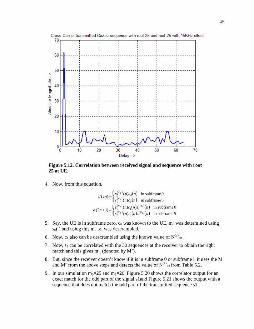
Figure 5.12. Correlation between received signal and sequence with root 25 at UE. .............45
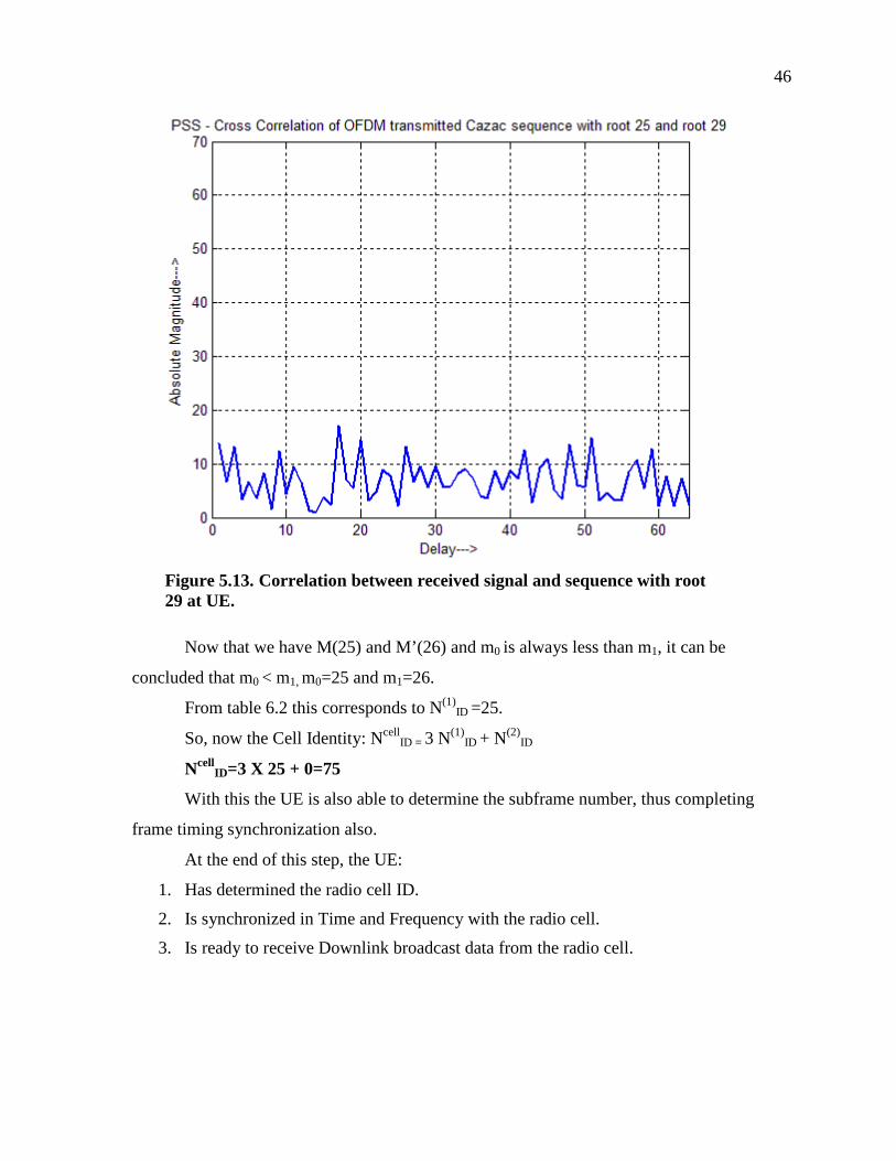
Figure 5.13. Correlation between received signal and sequence with root 29 at UE. .............46
Figure 5.14. Correlation between received signal and sequence with root 34 at UE. .............47
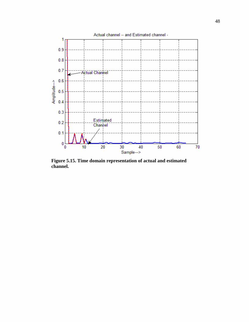
Figure 5.15. Time domain representation of actual and estimated channel.............................48
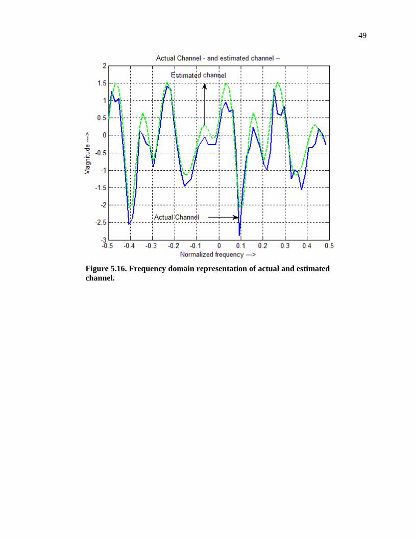
Figure 5.16. Frequency domain representation of actual and estimated channel. ...................49
Figure 5.17. SSS Detection block diagram. .............................................................................50
Figure 5.18. Correct match of signal with correlator for the de-interleaved even part. ...........51
Figure 5.19. Incorrect match of signal with correlator for the de-interleaved even part. ........52
Figure 5.20. Correct match for odd part of interleaved signal. ................................................53
Figure 5.21. Incorrect match for odd part of interleaved signal-peak is at an offset. ..............54
xi
ACKNOWLEDGEMENTS
I would like to whole heartedly thank Prof. fredric j.harris. His love for the subject
and passion to share his knowledge with students by explaining simply and clearly have
completely inspired and motivated me throughout the research and thesis process. He has
always been available to guide appropriately, answer questions and provide deeper insight
into the research study. I particularly thank him for all the time, support and encouragement
he had given me during this thesis. I would also like to thank Prof. Santosh Nagaraj and Prof.
Christopher Paolini for their valuable time serving on my thesis committee.

1
CHAPTER 1
INTRODUCTION
This Master’s Thesis presents in text and simulation, the cell search procedure, as
used by the Mobile Unit in 4G LTE systems. The cell search procedure begins when the
Mobile unit is powered on and it has to start communicating with the strongest base station.
This chapter presents some background information on the evolution of LTE.
We find ourselves in a generation where technology and gadgets have become an
integral part of our everyday life. We cannot imagine a day without laptops, mobile phones
and other gadgets like the iPod. Communication has matured a long way from being just a
means to communicate welfare to a stage where business and trade are being performed
online sitting at one place. This has been possible today thanks to the advancement in
communication and internet. Smart phones have merged so much into the wireless
communications industry that they have become an essential gadget in everyone’s life. With
the growing popularity of the smart phones and other mobile gadgets comes the need for
higher data transfer rates thus making Wireless Communications a constantly evolving field.
The first cellular system was developed by Nippon Telephone and Telegraph in Japan
in 1979. From here the ubiquitous cellular wireless communication system evolved. The first
generation cellular system was based on analog narrowband FM frequency division multiple
access. Spectrum efficiency was improved in second generation cellular with help of
improved digital communication techniques. The most common and widely used 2G systems
are CDMA (Code Division Multiple Access, IS-95) and GSM (Global System for Mobile
communications, originally Groupe Spécial Mobile) [1].
The next generation 3G system concept started in the mid-1980s as IMT200
(International Mobile Telecommunication). The 3G systems started with high commonality
of design with some basic key features including worldwide compatibility of services,
worldwide roaming, high speed internet and other multimedia applications. By the year 2000
two standards evolved for 3G systems, WCDMA (Wide Band CDMA) and UMTS
(Universal Mobile Telecommunication Systems). 3GPP Long Term Evolution (LTE) is a

2
standard in the mobile phone network technology tree that produced the GSM/EDGE and
UMTS/HSPA network technologies [1]. The world's first publicly available LTE-service
was opened by TeliaSonera in the two Scandinavian capitals Stockholm and Oslo on the 14th
of December 2009 [2].
In the further chapters, I would be presenting an overview of the evolution of LTE
and then proceed to the explanation of how the mobile unit performs cell search in LTE
systems.

3
CHAPTER 2
ORTHOGONAL FREQUENCY DIVISION
MULTIPLEXING
The need for high speed wireless applications at the cost of minimizing losses and
limited RF channel bandwidth have led to a need for the development of new power and
bandwidth efficient air interface schemes. The most spectral efficient scheme which has
gained popularity through 802.11 WLAN is the OFDM which has proved to be a foundation
for development of newer wireless air interface schemes.
The concept of OFDM has been around as early as 1960’s. The OFDM technique was
used in several high frequency military systems. In the 1980’s OFDM was studied for high
speed modems, digital mobile techniques for multiplexed QAM using DFT [3]. However
OFDM did reach its maturity for employment in wideband data communications over mobile
radio FM channels, high bit rate digital subscriber lines (HDSL; 1.6 Mbps) asymmetric
digital subscriber lines(ADSL; 6 Mbps), very high speed digital subscriber lines ( VDSL; 100
Mbps), Digital Audio Broadcasting (DAB), Terrestrial Broadcasting only during 1990’s [4].
The primary advantage of OFDM over single-carrier schemes is its ability to cope
with severe channel conditions (such as narrowband interference and frequency-selective
fading due to multipath) without complex equalization filters. Channel equalization is
simplified because OFDM may be viewed as using many slowly-modulated narrowband
signals rather than one rapidly-modulated wideband signal. The low symbol rate makes the
use of a guard interval between symbols affordable, making it possible to eliminate inter
symbol interference (ISI).
Frequency Division Multiplexing is one of the popular techniques used in Radio and
TV transmission. The frequency spectrum is divided into several logical channels, giving
each user an exclusive possession of the frequency band.

4
The basic approach is to divide the available bandwidth of a single physical medium
into a number of smaller, independent frequency channels. Figure 2.1 shows spectral
occupancy in a basic FDM system [5].
Figure 2.1. Spectral occupancy in FDM System.
OFDM is a special case of Frequency Division Multiplexing (FDM). OFDM is
frequency division multiplexing with a number of narrow band orthogonal sub carriers. The
main concept in OFDM is the orthogonality of the sub carriers.
The word Orthogonal in OFDM indicates the specific relationship between the
subcarriers in an OFDM system. The orthogonality of subcarriers is explained by Figure 2.2
[6]. Orthogonality can be achieved by carefully selecting carrier spacing, such as letting the
carrier spacing be equal to the reciprocal of the useful symbol period.
Figure 2.2. Orthogonality of OFDM subcarriers.
The peak of each carrier overlaps with the zeros of the remaining subcarriers so as to
minimize ISI. These orthogonal symbols can be separated at the receiver by correlation
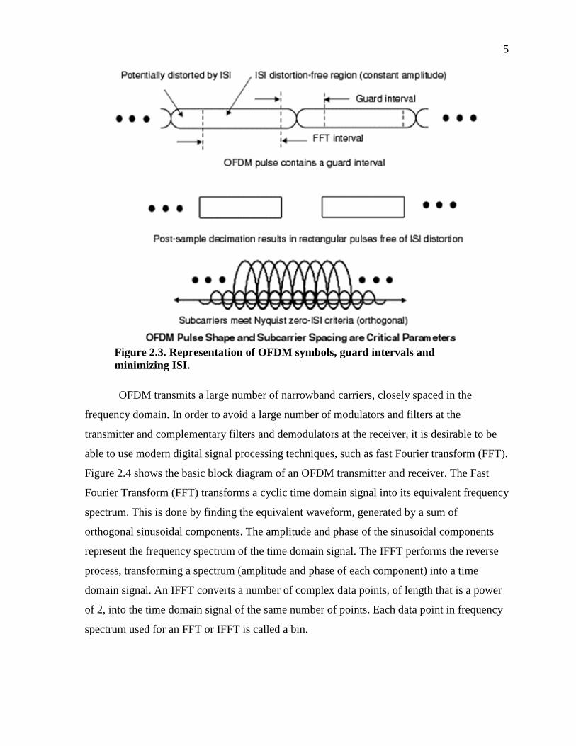
techniques; hence, Inter Symbol Interference among channels can be eliminated. Figure 2.3
shows how the presence of guard intervals in OFDM symbols generates a useful distortion
free region that can be used to recover data.
5
Figure 2.3. Representation of OFDM symbols, guard intervals and minimizing ISI.
OFDM transmits a large number of narrowband carriers, closely spaced in the
frequency domain. In order to avoid a large number of modulators and filters at the
transmitter and complementary filters and demodulators at the receiver, it is desirable to be
able to use modern digital signal processing techniques, such as fast Fourier transform (FFT).
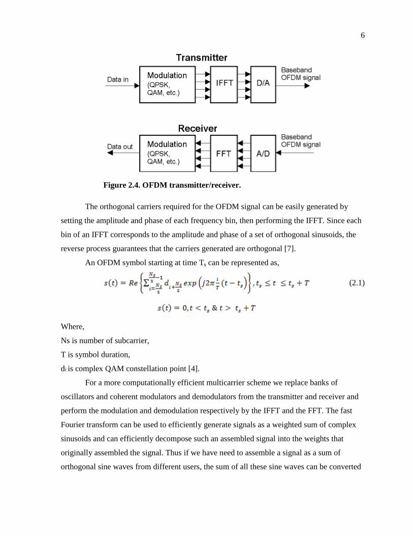
Figure 2.4 shows the basic block diagram of an OFDM transmitter and receiver. The Fast
Fourier Transform (FFT) transforms a cyclic time domain signal into its equivalent frequency
spectrum. This is done by finding the equivalent waveform, generated by a sum of
orthogonal sinusoidal components. The amplitude and phase of the sinusoidal components
represent the frequency spectrum of the time domain signal. The IFFT performs the reverse
process, transforming a spectrum (amplitude and phase of each component) into a time
domain signal. An IFFT converts a number of complex data points, of length that is a power
of 2, into the time domain signal of the same number of points. Each data point in frequency
spectrum used for an FFT or IFFT is called a bin.
6
Figure 2.4. OFDM transmitter/receiver.
The orthogonal carriers required for the OFDM signal can be easily generated by
setting the amplitude and phase of each frequency bin, then performing the IFFT. Since each
bin of an IFFT corresponds to the amplitude and phase of a set of orthogonal sinusoids, the
reverse process guarantees that the carriers generated are orthogonal [7].
An OFDM symbol starting at time Ts can be represented as,
(2.1)
Where,
Ns is number of subcarrier,
T is symbol duration,
di is complex QAM constellation point [4].
For a more computationally efficient multicarrier scheme we replace banks of
oscillators and coherent modulators and demodulators from the transmitter and receiver and
perform the modulation and demodulation respectively by the IFFT and the FFT. The fast
Fourier transform can be used to efficiently generate signals as a weighted sum of complex
sinusoids and can efficiently decompose such an assembled signal into the weights that
originally assembled the signal. Thus if we have need to assemble a signal as a sum of
orthogonal sine waves from different users, the sum of all these sine waves can be converted

7
into a single time signal by using an IFFT and then back to the amplitude of the individual
sine waves by using an FFT. Suppose the data to be transferred is,
,
At the transmitter, we perform and IFFT as shown here,
(2.2)
Where n belongs to the interval, [-N/2 to (N/2)-1].
At the receiver, we perform and FFT as shown here,
(2.3)
Where k belongs to the interval, [-N/2 to (N/2)-1].
One of the significant advantages of OFDM is in suppressing ISI. One of the main
factors causing ISI is distortion due to multipath. Multipath is generally caused by reflections
off objects such as buildings, vehicles and trees. Figure 2.5 shows an illustrative example of
multipath [8].
Figure 2.5. Multipath (Signal is reflected from various sources). Source: B. Schrick, and M. J. Riezenman, “Wireless Broadband in a Box,” IEEE Spectrum, vol. 39, no. 6, pp. 38-43, June 2002.

8
To mitigate the effects of Inter Symbol Interference (ISI) caused by channel delay
spread, each block of N IFFT coefficients is typically preceded by a cyclic prefix (CP) or a
guard interval consisting of Ng samples, such that the length of the CP is at least equal to the
channel length Nh in samples, where μ = (Th/Ts)N, Th is the length of (Continuous) channel,
and Ts is the duration of a OFDM block or symbol. Cyclic prefix is simply a repetition of the
last Ng IFFT coefficients. Alternatively, a cyclic suffix can be appended to the end of a block
of N IFFT coefficients that is a repetition of the first Ng IFFT coefficients [3].
2.1 TIME AND FREQUENCY SYNCHRONIZATION IN OFDM SYSTEMS
In order to demodulate an OFDM signal, the receiver needs to perform two important
synchronization tasks. First, Timing Synchronization -the timing offset of the symbol and the
optimal timing instants need to be properly determined. Second, Frequency Synchronization-
the receiver must align its carrier frequency as closely as possible with the transmitted carrier
frequency. The timing synchronization requirements are kind of relaxed when compared to
single carrier systems since OFDM structure is designed to accommodate an optimal level of
this error. Frequency synchronization however is of utmost importance since the
orthogonality of the signals depends on them being individually recognizable in the
frequency domain [9].
2.2 TIMING SYNCHRONIZATION The presence of cyclic prefix relaxes the effects of timing errors in OFDM. If perfect
synchronization is not maintained, it is still possible to tolerate a timing offset of τ seconds
without any degradation in performance, as long as 0≤τ≤Tm-Ts, where Ts is the guard
time(cyclic prefix duration), and Tm is the maximum channel delay spread. Here τ<0
corresponds to sampling earlier than the ideal instant whereas τ>0 is greater than the ideal
instant. As long as 0≤τ≤Tm-Ts the timing offset can be included by the channel estimator in
the complex gain estimate for each sub channel and the appropriate phase shift can be
applied without any loss in performance [9].
On the other hand, if the timing offset τ is not within the window 0≤τ≤Tm-Ts, ISI
occurs regardless of whether the phase shift is appropriately accounted for. For the case
where τ>0, the receiver loses some of the energy since only a delayed version of the symbols

9
is received and undesired energy from subsequent symbol is added to this symbol resulting in
erroneous detection. For the case where Tm-Ts < τ, desired energy is lost and energy from
preceding symbol is incorporated into this symbol [9].
2.3 FREQUENCY SYNCHRONIZATION The commonly represented form of subcarriers in OFDM is the sinc form, which is
represented as,
Which is pictorially represented in Figure 2.6:
Figure 2.6. OFDM orthogonal subcarriers.
Since the zero crossings of the frequency domain sinc pulses all line up, as long as the
frequency offset, δ=0, there is no interference between the carriers. In practice however, due
to mismatched oscillators at the transmitter and receiver end and Doppler shifts owing to
mobility the offset is never zero [9].
2.4 OBTAINING SYNCHRONIZATION Synchronization is generally obtained in OFDM based communication systems using
pilot symbol and cyclic prefix.
Known pilot symbols are transmitted at periodical intervals and since the receiver
knows what is transmitted, attaining time and frequency synchronization is easy, but at the
cost of surrendering some throughput. In the absence of pilot symbols, cyclic prefix which
also contains redundancy, can also be used to obtain time and frequency synchronization.

10
The pilot symbols periodically transmitted in the OFDM symbols are classified as
Long Preamble and Short Preamble. The function of each signal is as described [10]:
• Short Symbols
• Start of Frame Detection
• Signal Strength Indication
• Frequency Offset Resolution
• Long Symbols
• Channel Estimate
• Fine Time Resolution
• Distributed Pilots
• Carrier Tracking
• Sample Clock Tracking
OFDM has found its place in a wide variety of applications including:
• IEEE 802.11a, g, j, n (Wi-Fi) Wireless LANs
• IEEE 802.15.3a Ultra Wideband (UWB) Wireless PAN
• IEEE 802.16d, e (WiMAX), WiBro, and HiperMAN Wireless MANs
• IEEE 802.20 Mobile Broadband Wireless Access (MBWA)
• DVB (Digital Video Broadcast) terrestrial TV systems: DVB-T, DVB-H, T-DMB and ISDB-T
• DAB (Digital Audio Broadcast) systems: EUREKA 147, Digital Radio Mondiale,
• HD Radio, T-DMB and ISDB-TSB
• Flash-OFDM cellular systems
• 3GPP UMTS & 3GPP@ LTE (Long-Term Evolution), and 4G
11
CHAPTER 3
WAN CONTENDERS-LTE AND WIMAX
As the communications industry is busy formulating new standards to efficiently
deliver high speed broadband mobile access in a single air interface and network architecture
at low cost to operators and end users, two standards, IEEE 802.16 (WiMAX) and 3GPP
LTE are leading the pack towards forming the next-generation of mobile network standards.
This chapter presents an overview of both these technologies.
3.1 WIMAX WiMAX (Worldwide Interoperability for Microwave Access) is a broadband wireless
technology developed by the WiMAX forums and it is based on the 802.16 standard which
has the objective of providing high speed data transfers over the air. WiMAX is being
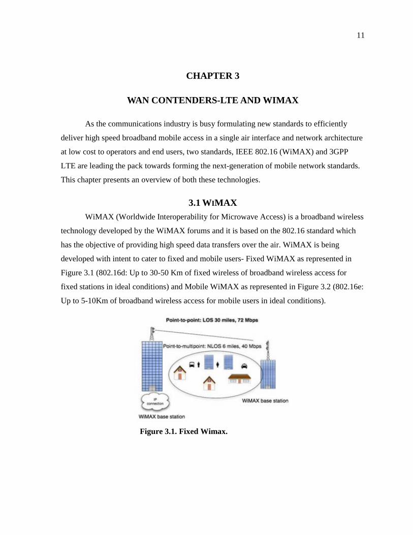
developed with intent to cater to fixed and mobile users- Fixed WiMAX as represented in
Figure 3.1 (802.16d: Up to 30-50 Km of fixed wireless of broadband wireless access for
fixed stations in ideal conditions) and Mobile WiMAX as represented in Figure 3.2 (802.16e:
Up to 5-10Km of broadband wireless access for mobile users in ideal conditions).
Figure 3.1. Fixed Wimax.
12
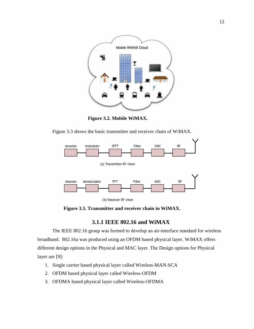
Figure 3.2. Mobile WiMAX.
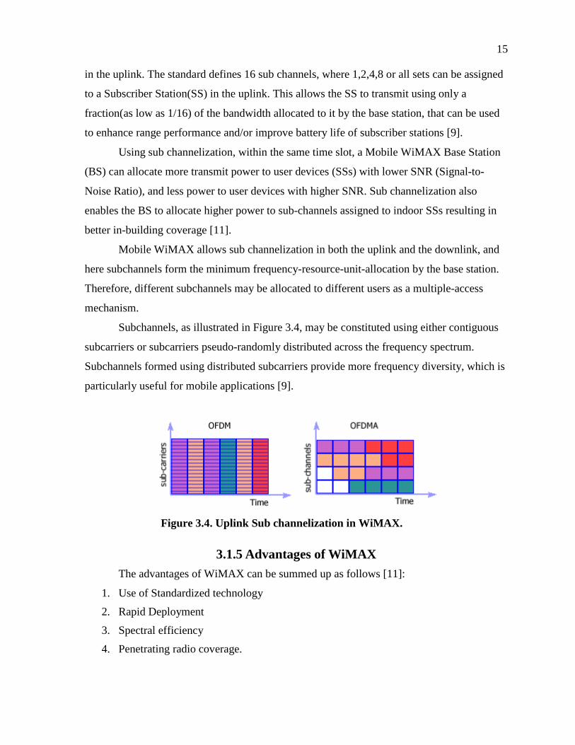
Figure 3.3 shows the basic transmitter and receiver chain of WiMAX.
Figure 3.3. Transmitter and receiver chain in WiMAX.
3.1.1 IEEE 802.16 and WiMAX The IEEE 802.16 group was formed to develop an air-interface standard for wireless
broadband. 802.16a was produced using an OFDM based physical layer. WiMAX offers
different design options in the Physical and MAC layer. The Design options for Physical
layer are [9]:
1. Single carrier based physical layer called Wireless-MAN-SCA
2. OFDM based physical layer called Wireless-OFDM
3. OFDMA based physical layer called Wireless-OFDMA

13
WiMAX supports both TDD(Time Division Duplexing) and FDD(Frequency
Division Duplexing). Currently there are two fixed WiMAX profiles against which
equipment have been certified. These are 3.5GHz systems operating over a 3.5 MHz channel,
based in IEEE 802.16-2004 OFDM physical layer. All mobile WiMAX profiles use scalable
OFDMA as the physical layer. All the current mobility certifications are TDD based [9].
3.1.2 Features of WiMAX Some of the important features of WiMAX are discussed here [9]:
Modulation supported by WiMAX: WiMAX supports the following formats in
downlink: BPSK,QPSK,16 QAM,64 QAM and supports the following formats in uplink:
BPSK,QPSK,16 QaM,64QAM.
High Peak data rates: The peak PHY data rat of WiMAX can be as high as 74Mbps
when using a 20MHz spectrum. Using 64 QAM in a 10 MHz spectrum operating using a
TDD scheme with 3:1 downlink-to-uplink ratio, the peak PHY data rate is about 25 Mbps
and 6.7 Mbps for downlink and uplink respectively.
OFDM Based PHY layer: The WiMAX PHY is based on OFDM which is known
for its good multi-path thus enabling WiMAX to operate in NLOS(Non Line-of-sight
conditions).
Scalable bandwidth and data rate support: The use of OFDM in the PHY layer
allows for the data rate to scale easily with available channel bandwidth. This is possible by
adjusting the FFT size. For example, a WiMAX system may use 128-, 512- or 1048-bit FFTs
based on whether the channel bandwidth is 1.25MHz, 5MHz or 10 MHz respectively. This
scaling may also be done dynamically.
Adaptive Modulation and Coding: WiMAX supports a number of Forward Error
Correcting Codes and allows the scheme to be changed on a frame by frame basis. This is an
effective mechanism to maximize throughput in a time-varying channel.
Support of TDD and FDD: IEEE 802.16-2004 and IEEE 802.16e-2005 supports
both Time Division Duplexing and Frequency Division Duplexing, as well as half-duplex
FDD.
Flexible and dynamic per user allocation: Both uplink and downlink resource
allocation are controlled by a scheduler at the base station. Capacity is shared among

14
multiple users on a demand basis, using a burst TDM scheme. The standard allows for
bandwidth resources to be allocated in Time, frequency and space and has a flexible
mechanism to convey the resource allocation information on a frame-by-frame basis.
Support for mobility: The mobile WiMAX has mechanisms to support secure
seamless handovers for delay-tolerant full-mobility applications, such as VoIP. The system
also has built-in support for power saving mechanisms that extend the battery life of
handheld subscriber devices. Physical layer enhancements such as more frequent channel
estimations, uplink sub channelization, and power control are also specified for mobile
applications.
3.1.3 OFDM Parameters in WiMAX The fixed and mobile versions of WiMAX have different implementations of the
OFDM Physical layer. Fixed WiMAX uses a 256 FFT-based OFDM Physical layer. Mobile
WiMAX, uses a scalable OFDMA physical layer in which the FFT sizes can vary from 128
bits to 2048 bits [9].
Table 3.1 shows a comparative analysis between the parameters used in Fixed and
Mobile WiMAX.
Table 3.1. Comparison between Fixed and Mobile WiMAX Parameter Fixed
WiMAX OFDM-PHY
Mobile WiMAX Scalable OFDMA-PHY
FFT Size 256 128 512 1024 2048 No. of used data subcarriers
192 72 360 720 1440
No. of pilot subcarriers 8 12 60 120 240 Number of guard band subcarriers
56 44 92 184 368
Channel BW 3.5 1,25 5 10 20 Subcarrier freq Spacing(kHz)
15.625 10.94 10.94 10.94 10.94
OFDM Symbol duration(micro seconds)
72 102.9 102.9 102.9 102.9
3.1.4 Subchannelization: OFDMA The available subcarriers may be divided into several groups of subcarriers called sub
channels. Fixed WiMAX based on OFDM-PHY allows a limited form of sub channelization
15
in the uplink. The standard defines 16 sub channels, where 1,2,4,8 or all sets can be assigned
to a Subscriber Station(SS) in the uplink. This allows the SS to transmit using only a
fraction(as low as 1/16) of the bandwidth allocated to it by the base station, that can be used
to enhance range performance and/or improve battery life of subscriber stations [9].
Using sub channelization, within the same time slot, a Mobile WiMAX Base Station
(BS) can allocate more transmit power to user devices (SSs) with lower SNR (Signal-to-
Noise Ratio), and less power to user devices with higher SNR. Sub channelization also
enables the BS to allocate higher power to sub-channels assigned to indoor SSs resulting in
better in-building coverage [11].
Mobile WiMAX allows sub channelization in both the uplink and the downlink, and
here subchannels form the minimum frequency-resource-unit-allocation by the base station.
Therefore, different subchannels may be allocated to different users as a multiple-access
mechanism.
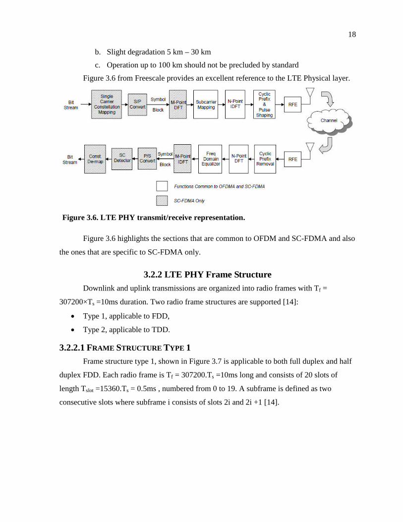
Subchannels, as illustrated in Figure 3.4, may be constituted using either contiguous
subcarriers or subcarriers pseudo-randomly distributed across the frequency spectrum.
Subchannels formed using distributed subcarriers provide more frequency diversity, which is
particularly useful for mobile applications [9].
Figure 3.4. Uplink Sub channelization in WiMAX.
3.1.5 Advantages of WiMAX The advantages of WiMAX can be summed up as follows [11]:
1. Use of Standardized technology
2. Rapid Deployment
3. Spectral efficiency
4. Penetrating radio coverage.

16
5. Scalability
6. Security
7. High Data throughput
8. Cost effectiveness.
3.2 LTE (LONG TERM EVOLUTION) This section provides an introduction to LTE systems and in the process highlights
the difference between LTE and WiMAX systems.
LTE is a wireless broadband technology designed to support roaming Internet access
via cell phones and handhelds. LTE is also referred to as 4G along with WiMAX because of
the significant improvements it offers. The goal of LTE is to provide a high-data-rate, low-
latency and packet-optimized radio-access technology.
LTE system supports flexible bandwidths thanks to OFDMA and SC-FDMA access
schemes. In addition to FDD(Frequency Division Duplexing) and TDD(Time Division
Duplexing), half duplex FDD is also allowed to support low cost UE. LTE system supports
peak data rates of 326 Mb/s with 4 X 4 MIMO within 20 MHz bandwidth. In terms of
latency, the LTE radio-interface and network provides capabilities for less than 10ms latency
for the transmission of a packet from network to UE [12]. OFDMA allows data to be directed
to or from multiple users on a subcarrier-by-subcarrier basis for a specified number of
symbol periods.
LTE differs significantly from WiMAX in the physical layer aspect that it uses SC-
FDMA for the uplink. SC-FDMA has shown to have much lower PAPR(Peak to Average
Power Ratio) when compared to OFDM which makes it a great choice for uplink
transmission in LTE.
Figure 3.5 represents the difference in the transmission scheme of OFDM and SC-
FDMA. The following section explains SC-FDMA in detail.
3.2.1 Design Goals of LTE The LTE Physical layer is designed to meet the following goals [13]:
1. Support scalable bandwidths of 1.25, 2.5, 5.0, 10.0 and 20.0 MHz
2. Peak data rate that scales with system bandwidth

17
Figure 3.5. OFDM and SC-FDMA transmission schemes.
a. Downlink (2 Ch MIMO) peak rate of 100 Mbps in 20 MHz channel
b. Uplink (single Ch Tx) peak rate of 50 Mbps in 20 MHz channel
3. Supported antenna configurations
a. Downlink: 4x2, 2x2, 1x2, 1x1
b. Uplink: 1x2, 1x1
4. Spectrum efficiency
a. Downlink: 3 to 4 x HSDPA Rel. 6
b. Uplink: 2 to 3 x HSUPA Rel. 6
5. Latency
a. C-plane: <50 – 100 msec to establish U-plane
b. U-plane: <10 msec from UE to server
6. Mobility
a. Optimized for low speeds (<15 km/hr)
b. High performance at speeds up to 120 km/hr
c. Maintain link at speeds up to 350 km/hr
7. Coverage
a. Full performance up to 5 km
18
b. Slight degradation 5 km – 30 km
c. Operation up to 100 km should not be precluded by standard
Figure 3.6 from Freescale provides an excellent reference to the LTE Physical layer.
Figure 3.6. LTE PHY transmit/receive representation.
Figure 3.6 highlights the sections that are common to OFDM and SC-FDMA and also
the ones that are specific to SC-FDMA only.
3.2.2 LTE PHY Frame Structure Downlink and uplink transmissions are organized into radio frames with Tf =
307200×Ts =10ms duration. Two radio frame structures are supported [14]:
• Type 1, applicable to FDD,
• Type 2, applicable to TDD.
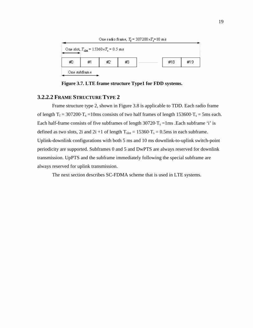
3.2.2.1 FRAME STRUCTURE TYPE 1 Frame structure type 1, shown in Figure 3.7 is applicable to both full duplex and half
duplex FDD. Each radio frame is Tf = 307200.Ts =10ms long and consists of 20 slots of
length Tslot =15360.Ts = 0.5ms , numbered from 0 to 19. A subframe is defined as two
consecutive slots where subframe i consists of slots 2i and 2i +1 [14].
19
Figure 3.7. LTE frame structure Type1 for FDD systems.
3.2.2.2 FRAME STRUCTURE TYPE 2 Frame structure type 2, shown in Figure 3.8 is applicable to TDD. Each radio frame
of length Tf = 307200⋅Ts =10ms consists of two half frames of length 153600⋅Ts = 5ms each.
Each half-frame consists of five subframes of length 30720⋅Ts =1ms .Each subframe ‘i’ is
defined as two slots, 2i and 2i +1 of length Tslot = 15360⋅Ts = 0.5ms in each subframe.
Uplink-downlink configurations with both 5 ms and 10 ms downlink-to-uplink switch-point
periodicity are supported. Subframes 0 and 5 and DwPTS are always reserved for downlink
transmission. UpPTS and the subframe immediately following the special subframe are
always reserved for uplink transmission.
The next section describes SC-FDMA scheme that is used in LTE systems.

20
One
slo
t, T
slot
=15
360T
s
GP
UpP
TS
Dw
PT
S
One
rad
io fr
ame,
Tf =
307
200T
s =
10
ms
One
hal
f-fr
ame,
153
600 T
s =
5 m
s
3072
0Ts
One
su
bfra
me,
30
720T
s
GP
UpP
TS
Dw
PT
S
Sub
fram
e #2
Sub
fram
e #3
Sub
fram
e #4
Sub
fram
e #0
Sub
fram
e #5
Sub
fram
e #7
Sub
fram
e #8
Sub
fram
e #9
Figu
re 3
.8. L
TE
fram
e st
ruct
ure
Typ
e2 fo
r T
DD
syst
ems.
21
CHAPTER 4
SC-FDMA
In cellular applications, the principal advantage of using OFDMA is its robustness in
the presence of multipath signal propagation [4]. This robustness of OFDMA against
multipath is due to the fact that OFDMA splits data into N subcarrier and thus each carrier
occupies 1/N-th of the available bandwidth and occupies a time span equal to N times the
time span of each input signal data symbol time duration. However OFDMA waveform
exhibits very pronounced envelop fluctuations resulting in high PAPR (Peak Average Power
Ratio), because of large PAPR, high linear amplifiers are required in the system. High linear
amplifiers usually have low power efficiency as they have to operate on large range [15].
The goal for the LTE uplink access scheme design is to provide low signal peakiness
comparable to WCDMA signal peakiness while providing orthogonal access not requiring an
SIC (Successive Interference Cancellation) receiver [12]. LTE systems use SC-FDMA
(Single Carrier Frequency Division Multiple Access) in the LTE uplink to cater to this
requirement. SC-FDMA systems have shown to have low PAPR when compared to OFDM.
SC-FDMA provides orthogonal access to multiple users simultaneously accessing the
system [12]. In SC-FDMA, the data sequence is FFT precoded and this FFT-precoded
sequence is mapped to uniformly spaced subcarriers at the input of the IFFT. This mapping
of FFT-precoded sequence onto IFFT can be performed in two ways: Distributed mapping
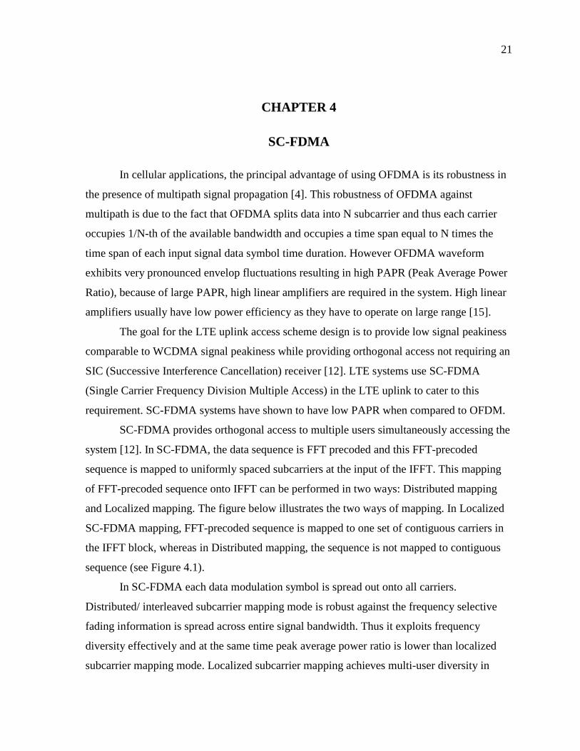
and Localized mapping. The figure below illustrates the two ways of mapping. In Localized
SC-FDMA mapping, FFT-precoded sequence is mapped to one set of contiguous carriers in
the IFFT block, whereas in Distributed mapping, the sequence is not mapped to contiguous
sequence (see Figure 4.1).
In SC-FDMA each data modulation symbol is spread out onto all carriers.
Distributed/ interleaved subcarrier mapping mode is robust against the frequency selective
fading information is spread across entire signal bandwidth. Thus it exploits frequency
diversity effectively and at the same time peak average power ratio is lower than localized
subcarrier mapping mode. Localized subcarrier mapping achieves multi-user diversity in
22
Figure 4.1. Localized mapping and Distributed mapping.
presence of frequency selective fading as user can be assigned subcarrier according to their
channel gain.
As a beginning of this research work, transmit and receive of SC-FDMA data
between two users, User A and User B was performed using CAZAC sequences for channel
estimation. The channel was estimated using Zadoff-Chu (CAZAC sequences) and this
channel was undone at the receiver end. Localized subcarrier mapping was used.
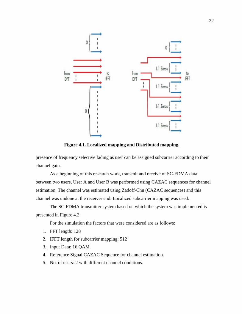
The SC-FDMA transmitter system based on which the system was implemented is
presented in Figure 4.2.
For the simulation the factors that were considered are as follows:
1. FFT length: 128 2. IFFT length for subcarrier mapping: 512
3. Input Data: 16 QAM.
4. Reference Signal CAZAC Sequence for channel estimation.
5. No. of users: 2 with different channel conditions.
23
Figure 4.2. SC-FDMA transmitter.
In the case of localized SC-FDMA the inputs to IFFT are given as,
X'l= Xl 0 ≤ l ≤ M-1
0 M ≤ l ≤ N-1
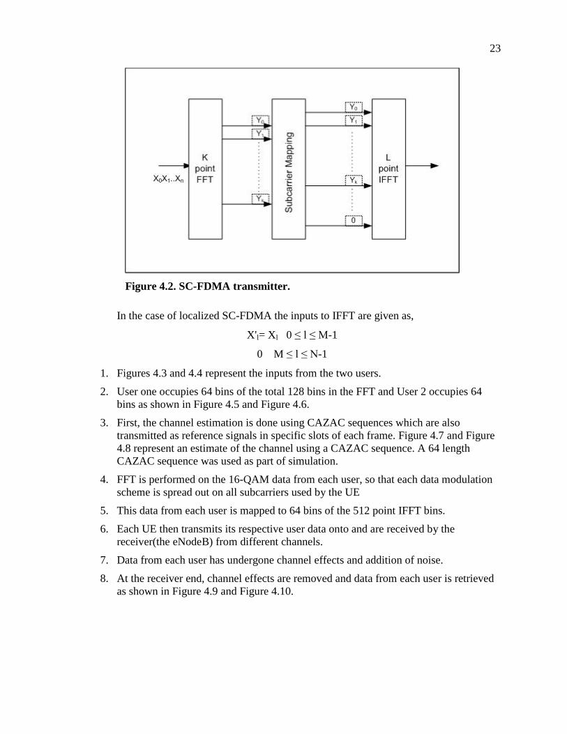
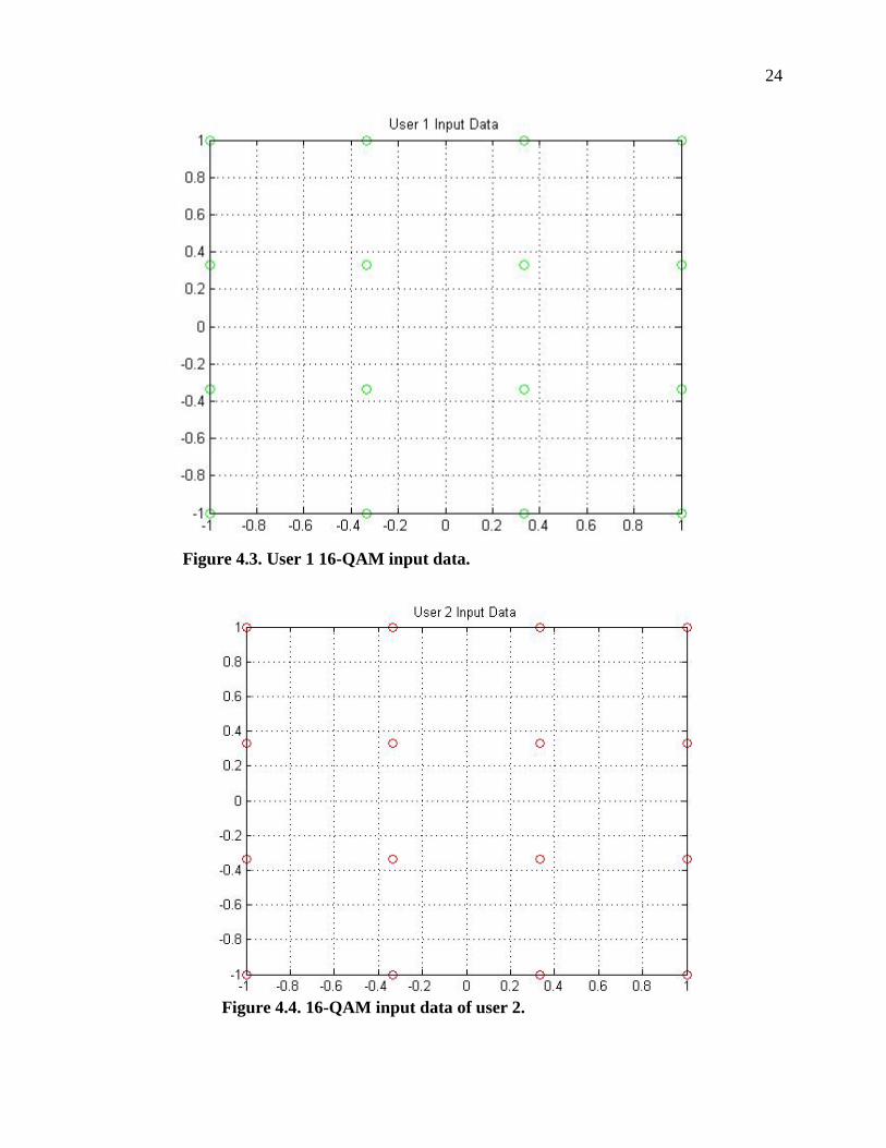
1. Figures 4.3 and 4.4 represent the inputs from the two users.
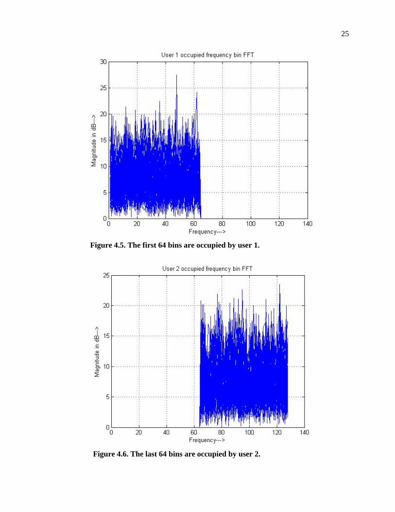
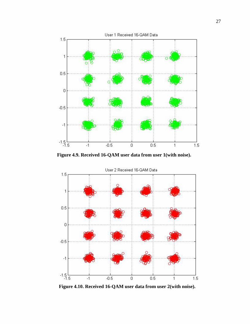
2. User one occupies 64 bins of the total 128 bins in the FFT and User 2 occupies 64 bins as shown in Figure 4.5 and Figure 4.6.
3. First, the channel estimation is done using CAZAC sequences which are also transmitted as reference signals in specific slots of each frame. Figure 4.7 and Figure 4.8 represent an estimate of the channel using a CAZAC sequence. A 64 length CAZAC sequence was used as part of simulation.
4. FFT is performed on the 16-QAM data from each user, so that each data modulation scheme is spread out on all subcarriers used by the UE
5. This data from each user is mapped to 64 bins of the 512 point IFFT bins.
6. Each UE then transmits its respective user data onto and are received by the receiver(the eNodeB) from different channels.
7. Data from each user has undergone channel effects and addition of noise.
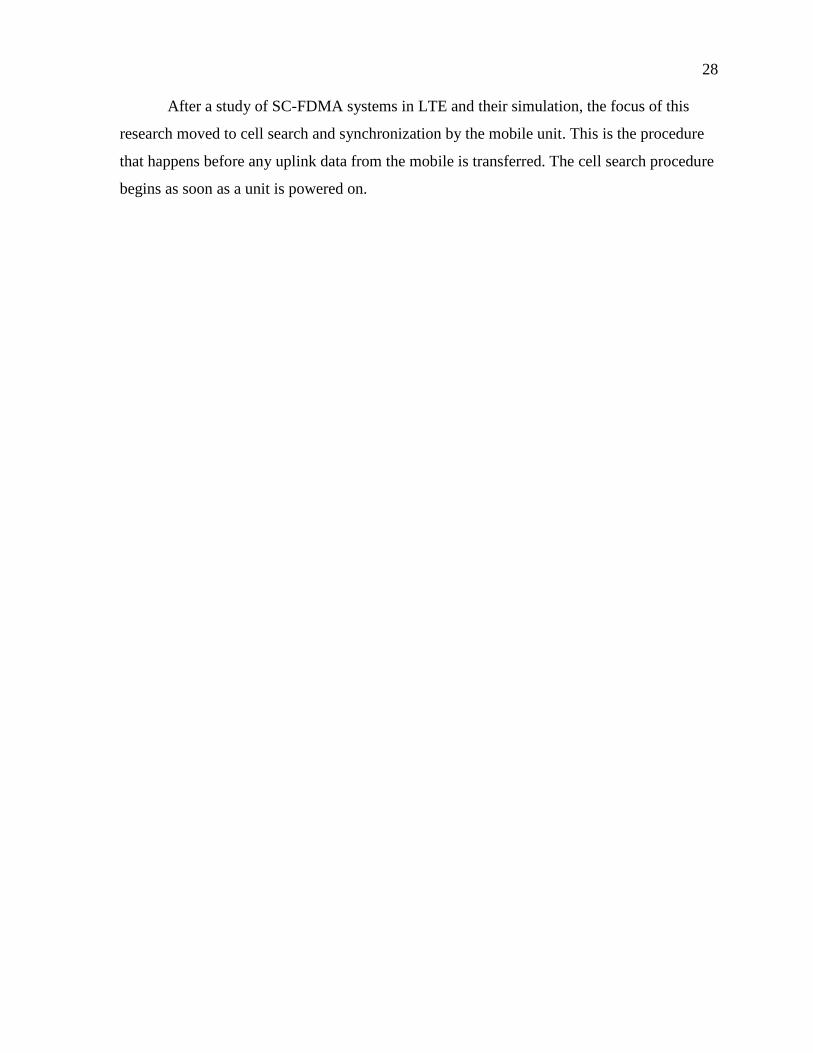
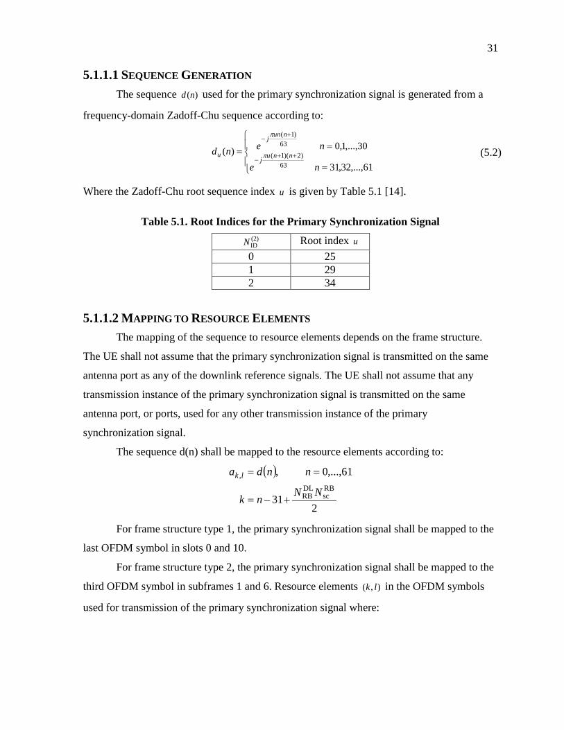
8. At the receiver end, channel effects are removed and data from each user is retrieved as shown in Figure 4.9 and Figure 4.10.
24
Figure 4.3. User 1 16-QAM input data.
Figure 4.4. 16-QAM input data of user 2.
25
Figure 4.5. The first 64 bins are occupied by user 1.
Figure 4.6. The last 64 bins are occupied by user 2.

26
Figure 4.7. Channel estimation by user 1.
Figure 4.8. Channel estimation by user 2.
27
Figure 4.9. Received 16-QAM user data from user 1(with noise).
Figure 4.10. Received 16-QAM user data from user 2(with noise).
28
After a study of SC-FDMA systems in LTE and their simulation, the focus of this
research moved to cell search and synchronization by the mobile unit. This is the procedure
that happens before any uplink data from the mobile is transferred. The cell search procedure
begins as soon as a unit is powered on.

29
CHAPTER 5
MOBILE CELL SEARCH AND
SYNCHRONIZATION
When an LTE mobile unit is powered on, it has to search for the available radio cells
and lock to one of them to continue further communication. Multiple mobile unit users
simultaneously try to access the same set of radio cells and also, the UE mobile unit begins it
search blindly without any knowledge of the bandwidth it has allocated. Hence the initial cell
search procedure must also be implemental in timing and frequency synchronization. This
research presents how a LTE mobile unit performs this cell search and identifies the strongest
available radio cell near it. The timing and frequency synchronization that is required as part
of this cell search procedure is also performed.
Cell Search is a basic function of any cellular system, during which timing and
frequency synchronization is obtained between the mobile unit and the network. Successful
execution of the cell search and selection procedure as well as acquiring initial system
information is essential for the UE before taking further steps to communicate with the
network. LTE uses a hierarchical cell-search procedure in which an LTE radio cell is
identified by a cell identity.
LTE systems consist of 504 unique physical layer cell identities. To accommodate
and manage this large amount, the cell identities are divided into 168 unique cell layer
identity groups. Each group further consists of three physical layer identities. A pictorial
representation of Hierarchical Cell identities is shown in Figure 5.1.
This is usually represented as: N(1)ID=0….167 and N(2)
ID=0,1,2.
And Cell Identity: NcellID = 3 N(1)
ID + N(2)ID
5.1 SYNCHRONIZATION SIGNALS This hierarchical cell search procedure is performed in two steps using two signals:
1. Primary Synchronization Signal and
2. Secondary Synchronization Signal.

30
Figure 5.1. Pictorial representation of hierarchical cell search.
The synchronization signals have 72 subcarriers reserved for them, but they use only
62 of the 72 subcarriers. The reason only 62 subcarriers are used is because it enables the UE
to perform 64 point FFT and lower sampling rate [16].
The Primary Synchronization signal first determines one of three cell identities (0, 1,
2), also represented by N(2)ID. Then the secondary synchronization signal, is used to determine
a cell ID between 0 and 167 represented by N(1)ID. The primary signal is based on Zadoff-Chu
sequence which is a Constant Amplitude Zero Auto Correlation (CAZAC) sequence.
A Zadoff-Chu sequence is a complex-valued mathematical sequence which exhibits
the useful property that cyclically shifted versions of it are orthogonal to each other.
The complex value at each position (n) of each root Zadoff–Chu sequence (u) given
by,
(5.1)
Where 0 <=n<=NZC-1,NZC = length of sequence. [17]
5.1.1 Primary Synchronization Signal This section describes in detail the generation and resource allocation of the Primary
Synchronization signal. The Primary Synchronization Signals are modulated using one of
three different frequency domain Zadoff-Chu sequences.
31
5.1.1.1 SEQUENCE GENERATION The sequence )(nd used for the primary synchronization signal is generated from a
frequency-domain Zadoff-Chu sequence according to:
=
== ++−
+−
61,...,32,31
30,...,1,0)(63
)2)(1(
63)1(
ne
nend nnuj
nunj
u π
π
(5.2)
Where the Zadoff-Chu root sequence index u is given by Table 5.1 [14].
Table 5.1. Root Indices for the Primary Synchronization Signal (2)IDN Root index u 0 25 1 29 2 34
5.1.1.2 MAPPING TO RESOURCE ELEMENTS The mapping of the sequence to resource elements depends on the frame structure.
The UE shall not assume that the primary synchronization signal is transmitted on the same
antenna port as any of the downlink reference signals. The UE shall not assume that any
transmission instance of the primary synchronization signal is transmitted on the same
antenna port, or ports, used for any other transmission instance of the primary
synchronization signal.
The sequence d(n) shall be mapped to the resource elements according to:
( )
231
61,...,0 ,RBsc
DLRB
,
NNnk
nnda lk
+−=
==
For frame structure type 1, the primary synchronization signal shall be mapped to the
last OFDM symbol in slots 0 and 10.
For frame structure type 2, the primary synchronization signal shall be mapped to the
third OFDM symbol in subframes 1 and 6. Resource elements ),( lk in the OFDM symbols
used for transmission of the primary synchronization signal where:
32
66,...63,62,1,...,4,52
31RBsc
DLRB
−−−=
+−=
n
NNnk
are reserved and not used for transmission of the primary synchronization signal [14].
NOTE: When mapping the PSS to resource elements, center element is left zero to
represent the DC component.
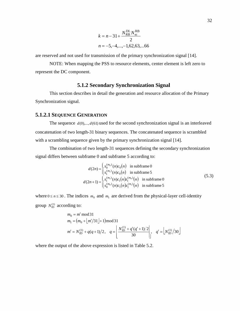
5.1.2 Secondary Synchronization Signal This section describes in detail the generation and resource allocation of the Primary
Synchronization signal.
5.1.2.1 SEQUENCE GENERATION The sequence )61(),...,0( dd used for the second synchronization signal is an interleaved
concatenation of two length-31 binary sequences. The concatenated sequence is scrambled
with a scrambling sequence given by the primary synchronization signal [14].
The combination of two length-31 sequences defining the secondary synchronization
signal differs between subframe 0 and subframe 5 according to:
( )( )( ) ( )( ) ( )
=+
=
5 subframein )(0 subframein )()12(
5 subframein )(0 subframein )()2(
)(11
)(0
)(11
)(1
0)(
1
0)(
0
10
01
1
0
nzncnsnzncnsnd
ncnsncnsnd
mm
mm
m
m
(5.3)
where 300 ≤≤ n . The indices 0m and 1m are derived from the physical-layer cell-identity
group (1)IDN according to:
( )
30,30
2)1(,2)1(
31mod13131mod
(1)ID
(1)ID(1)
ID
01
0
NqqqN
qqqNm
mmmmm
=′
+′′+=++=′
+′+=
′=
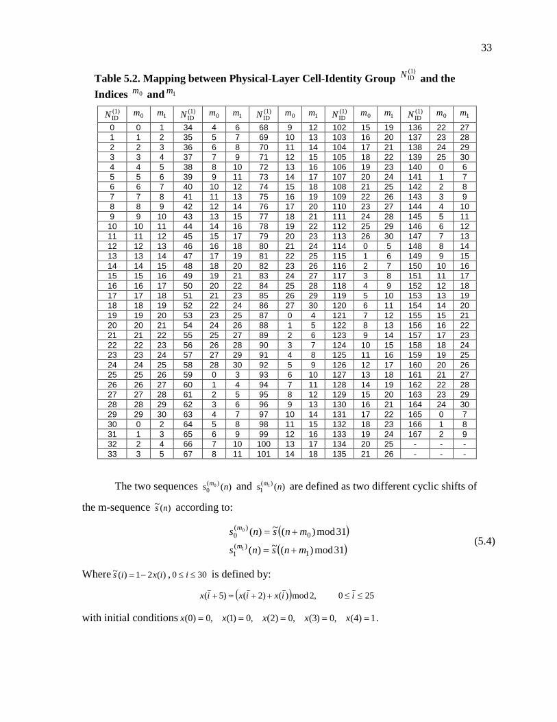
where the output of the above expression is listed in Table 5.2.
33
Table 5.2. Mapping between Physical-Layer Cell-Identity Group (1)IDN and the
Indices 0m and 1m (1)IDN 0m 1m
(1)IDN 0m 1m
(1)IDN 0m 1m
(1)IDN 0m 1m
(1)IDN 0m 1m
0 0 1 34 4 6 68 9 12 102 15 19 136 22 27 1 1 2 35 5 7 69 10 13 103 16 20 137 23 28 2 2 3 36 6 8 70 11 14 104 17 21 138 24 29 3 3 4 37 7 9 71 12 15 105 18 22 139 25 30 4 4 5 38 8 10 72 13 16 106 19 23 140 0 6 5 5 6 39 9 11 73 14 17 107 20 24 141 1 7 6 6 7 40 10 12 74 15 18 108 21 25 142 2 8 7 7 8 41 11 13 75 16 19 109 22 26 143 3 9 8 8 9 42 12 14 76 17 20 110 23 27 144 4 10 9 9 10 43 13 15 77 18 21 111 24 28 145 5 11 10 10 11 44 14 16 78 19 22 112 25 29 146 6 12 11 11 12 45 15 17 79 20 23 113 26 30 147 7 13 12 12 13 46 16 18 80 21 24 114 0 5 148 8 14 13 13 14 47 17 19 81 22 25 115 1 6 149 9 15 14 14 15 48 18 20 82 23 26 116 2 7 150 10 16 15 15 16 49 19 21 83 24 27 117 3 8 151 11 17 16 16 17 50 20 22 84 25 28 118 4 9 152 12 18 17 17 18 51 21 23 85 26 29 119 5 10 153 13 19 18 18 19 52 22 24 86 27 30 120 6 11 154 14 20 19 19 20 53 23 25 87 0 4 121 7 12 155 15 21 20 20 21 54 24 26 88 1 5 122 8 13 156 16 22 21 21 22 55 25 27 89 2 6 123 9 14 157 17 23 22 22 23 56 26 28 90 3 7 124 10 15 158 18 24 23 23 24 57 27 29 91 4 8 125 11 16 159 19 25 24 24 25 58 28 30 92 5 9 126 12 17 160 20 26 25 25 26 59 0 3 93 6 10 127 13 18 161 21 27 26 26 27 60 1 4 94 7 11 128 14 19 162 22 28 27 27 28 61 2 5 95 8 12 129 15 20 163 23 29 28 28 29 62 3 6 96 9 13 130 16 21 164 24 30 29 29 30 63 4 7 97 10 14 131 17 22 165 0 7 30 0 2 64 5 8 98 11 15 132 18 23 166 1 8 31 1 3 65 6 9 99 12 16 133 19 24 167 2 9 32 2 4 66 7 10 100 13 17 134 20 25 - - - 33 3 5 67 8 11 101 14 18 135 21 26 - - -
The two sequences )()(0
0 ns m and )()(1
1 ns m are defined as two different cyclic shifts of
the m-sequence )(~ ns according to:
( )( )31mod)(~)(
31mod)(~)(
1)(
1
0)(
0
1
0
mnsns
mnsnsm
m
+=
+=
(5.4)
Where )(21)(~ ixis −= , 300 ≤≤ i is defined by:
( ) 250 ,2mod)()2()5( ≤≤++=+ iixixix
with initial conditions 1)4(,0)3(,0)2(,0)1(,0)0( ===== xxxxx .
34
The two scrambling sequences )(0 nc and )(1 nc depend on the primary synchronization
signal and are defined by two different cyclic shifts of the m-sequence )(~ nc according to:
)31mod)3((~)(
)31mod)((~)()2(
ID1
)2(ID0
++=
+=
Nncnc
Nncnc
(5.5)
Where { }2,1,0)2(ID ∈N is the physical-layer identity within the physical-layer cell identity group
(1)IDN and )(21)(~ ixic −= , 300 ≤≤ i is defined by:
( ) 250 ,2mod)()3()5( ≤≤++=+ iixixix
with initial conditions 1)4(,0)3(,0)2(,0)1(,0)0( ===== xxxxx .
The scrambling sequences )()(1
0 nz m and )()(1
1 nz m are defined by a cyclic shift of the m-
sequence )(~ nz according to:
)31mod))8mod(((~)( 0)(
10 mnznz m +=
)31mod))8mod(((~)( 1)(
11 mnznz m += (5.6)
Where 0m and 1m are obtained from Table 5.2 and )(21)(~ ixiz −= , 300 ≤≤ i is defined by
( ) 250 ,2mod)()1()2()4()5( ≤≤++++++=+ iixixixixix
with initial conditions 1)4(,0)3(,0)2(,0)1(,0)0( ===== xxxxx .
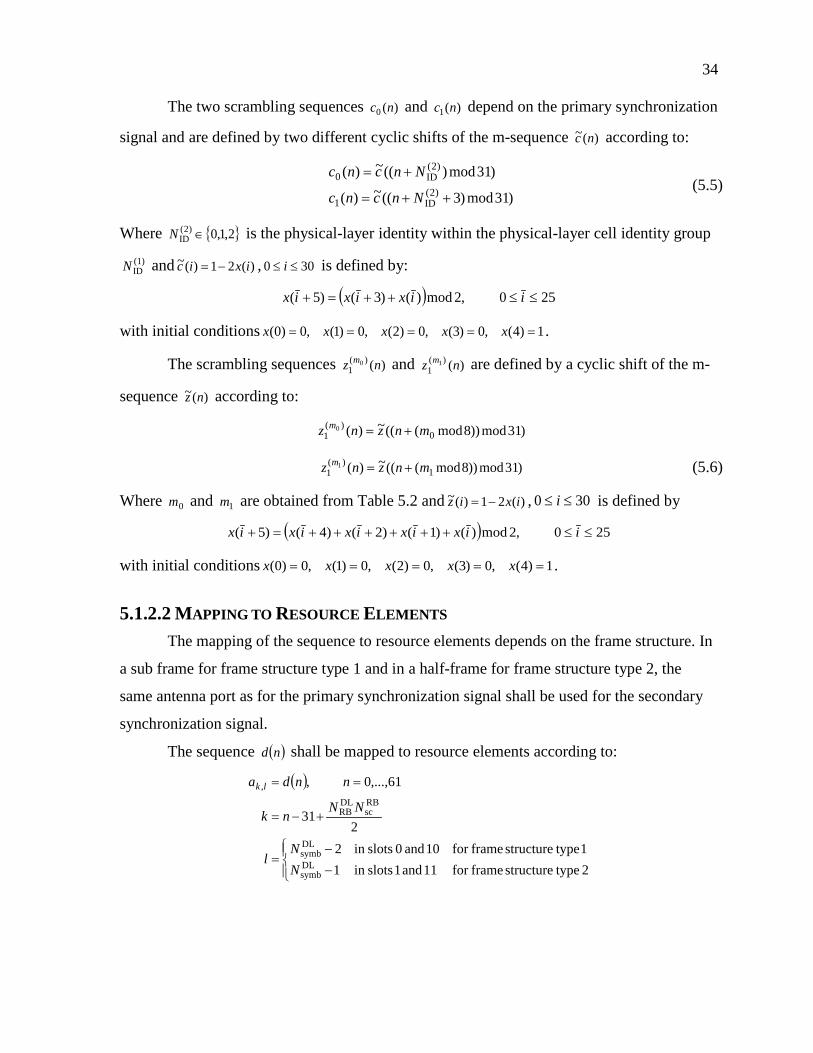
5.1.2.2 MAPPING TO RESOURCE ELEMENTS The mapping of the sequence to resource elements depends on the frame structure. In
a sub frame for frame structure type 1 and in a half-frame for frame structure type 2, the
same antenna port as for the primary synchronization signal shall be used for the secondary
synchronization signal.
The sequence ( )nd shall be mapped to resource elements according to:
( )
−
−=
+−=
==
2 typestructure framefor 11 and 1 slotsin 11 typestructure framefor 10 and 0 slotsin 2
231
61,...,0 ,
DLsymb
DLsymb
RBsc
DLRB
,
NN
l
NNnk
nnda lk

35
Resource elements ),( lk where:
66,...63,62,1,...,4,5
2 typestructure framefor 11 and 1 slotsin 11 typestructure framefor 10 and 0 slotsin 2
231
DLsymb
DLsymb
RBsc
DLRB
−−−=
−
−=
+−=
n
NN
l
NNnk
are reserved and not used for transmission of the secondary synchronization signal [14].
5.2 CELL SEARCH PROCEDURE Section 5.1 detailed the two synchronization signals that aid in cell search. The
detailed procedure of performing cell search and synchronization using these signals is
described in this section.
Firstly as soon as the UE (User Equipment) is switched on, it starts searching for a
strong cell in the Downlink band. Regardless of the bandwidth capability of the UE, it
generally searches in the central part of the bandwidth.
When the UE thinks it has found a good candidate with the required 72 subcarriers
(which are possibly the synch signals), the UE initially performs a rough frequency
synchronization. Since the PSS (Primary Synchronization Signal) is mapped to resource
elements after puncturing the DC element, the UE can look for the DC component and its
surrounding subcarriers to perform the rough synchronization.
The problems that the UE encounters and overcomes during initial startup are
simulated in this section and they are:
1. UE has to determine symbol start.
2. UE has to look for a cell and perform rough synchronization.
3. UE has to determine the carrier frequency.
4. UE has to perform timing synchronization.
5. UE has to perform fine frequency synchronization.
How these issues are encountered and resolved is schematically explained. This
assumes an FDD transmission scheme.
To begin with here is the MATLAB representation of the three primary
synchronization signals (see Appendix for MATLAB code to generate PSS). As described in
5.1.1, the PSS signals are Zadoff-chu sequences with their center made zero to represent DC.
36
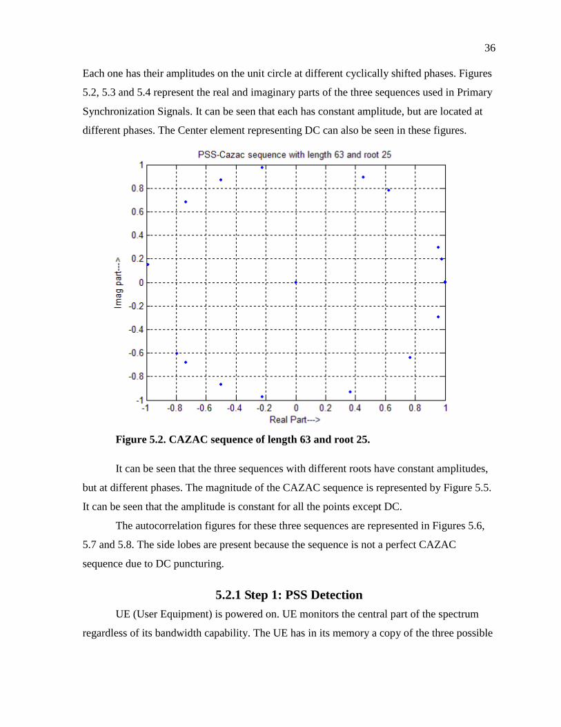
Each one has their amplitudes on the unit circle at different cyclically shifted phases. Figures
5.2, 5.3 and 5.4 represent the real and imaginary parts of the three sequences used in Primary
Synchronization Signals. It can be seen that each has constant amplitude, but are located at
different phases. The Center element representing DC can also be seen in these figures.
Figure 5.2. CAZAC sequence of length 63 and root 25.
It can be seen that the three sequences with different roots have constant amplitudes,
but at different phases. The magnitude of the CAZAC sequence is represented by Figure 5.5.
It can be seen that the amplitude is constant for all the points except DC.
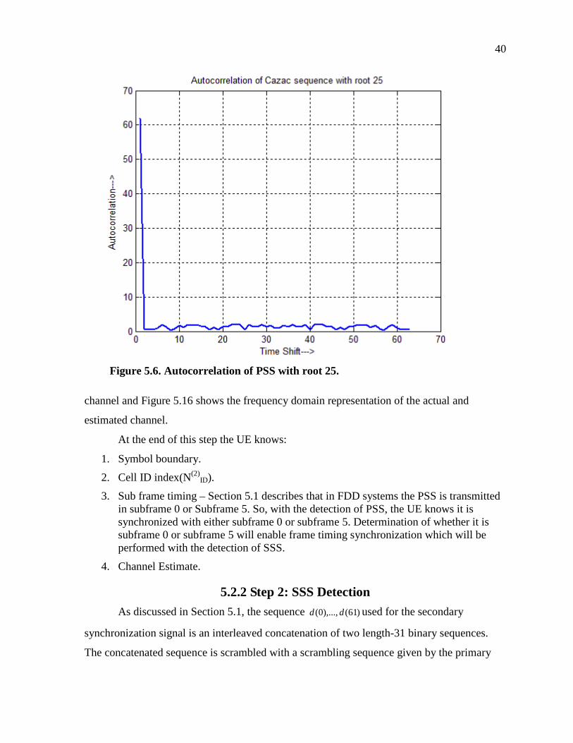
The autocorrelation figures for these three sequences are represented in Figures 5.6,
5.7 and 5.8. The side lobes are present because the sequence is not a perfect CAZAC
sequence due to DC puncturing.
5.2.1 Step 1: PSS Detection UE (User Equipment) is powered on. UE monitors the central part of the spectrum
regardless of its bandwidth capability. The UE has in its memory a copy of the three possible

37
Figure 5.3. CAZAC sequence of length 63 and root 29.
Primary Synchronization signals. The first step that a UE has to perform before proceeding
with further signal processing is the determination of the symbol start. The UE performs this
detection by using a sliding window method with a delay length of symbol length (here 64).
In this method, the received signal is processed with a delayed version of itself- the ratio of
the aggregated cross correlation(between the input to the delay line and the output to the
delay line) to the aggregated auto correlation at the output of the delay over a set of samples
helps in detecting the symbol start.
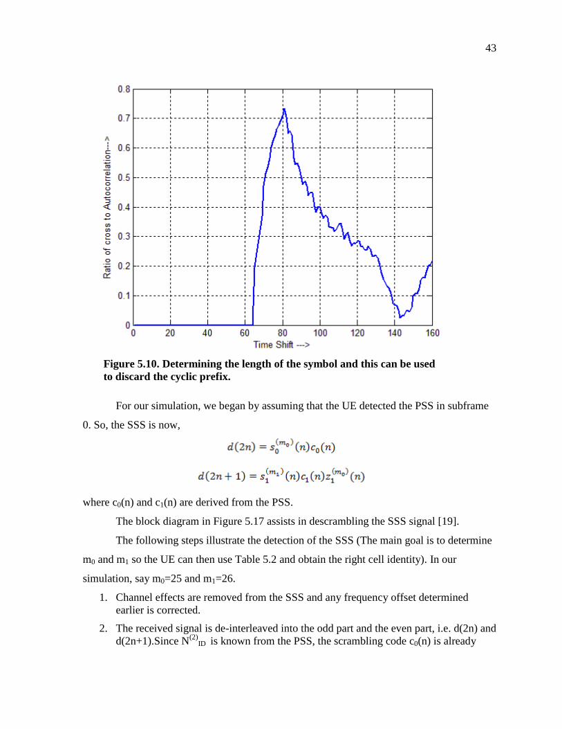
The symbol start is determined by checking the peak triangle in the ratio of the cross
and auto correlation as described in Figure 5.9. Figure 5.10 shows the peak that was obtained
at the symbol start.
From the MATLAB figure (Figure 5.10), the UE sees the peak at the 80th symbol, it
knows that the symbol start is after the 80th symbol.

38
Figure 5.4. CAZAC sequence of length 63 and root 34.
Now the UE has to match the received signal to one of the three sequences it knows.
The UE has to perform this with two considerations:
1. The signal has gone through a phase rotation while travelling from the radio cell to the UE.
2. The signal has undergone degradation due to the channel and the UE has to estimate the channel for use with the Secondary Synchronization Signal.
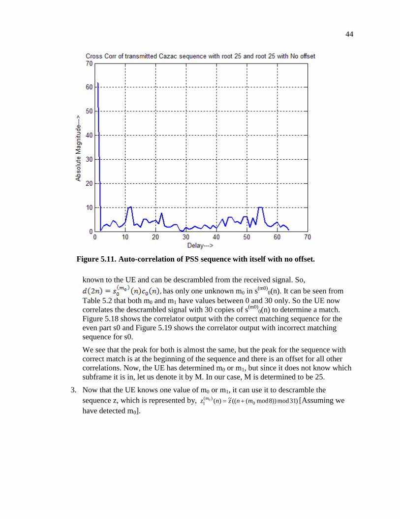
For simulation, it was assumed that the PSS with root 25 is the transmitted signal
from the radio cell. Figure 5.11 shows the correlation results at the receiver when there is an
exact match in sequence and there is no frequency offset. Figure 5.12 shows the correlation
results at the receiver when there is an exact match of the sequence with a 15 KHz offset.
Figure 5.13 and 5.14 shows the correlation results at the receiver when there is no exact
match.
It is evident from Figures 5.11-5.14 that the correlation amplitude maximum is
obtained only when the received sequence matches with one of the sequences. The UE has
determined which PSS the radio cell is transmitting (in this case, N(2)ID is 0 from Table 5.1).

39
Figure 5.5. Constant magnitude of PSS.
Also, the UE knows the position of the amplitude maximum peak when there is no offset and
depending on the position of the peak it finds when it detects the PSS it is able to calculate
the offset. In this case, it was determined that for every 15 kHz frequency offset, the peak
moves by one frequency bin. Now, the UE has determined the offset that it has to adjust
when it receives the SSS. Now, that the UE knows which PSS sequence is being received and
it has a known reference of the signal and has also determined any frequency offset, the UE
can now estimate the channel using its known reference of the original signal.
If the transmitted sequence is X, the received sequence is Y after channel effects, and
the channel is denoted by H, in frequency domain,
Y=XH and the channel H can be determined to be
H=Y/X.
The inverse of this known estimate of the channel can then substituted in the received
sequence. Figure 5.15 shows the time domain representation of the actual and estimated
40
Figure 5.6. Autocorrelation of PSS with root 25.
channel and Figure 5.16 shows the frequency domain representation of the actual and
estimated channel.
At the end of this step the UE knows:
1. Symbol boundary.
2. Cell ID index(N(2)ID).
3. Sub frame timing – Section 5.1 describes that in FDD systems the PSS is transmitted in subframe 0 or Subframe 5. So, with the detection of PSS, the UE knows it is synchronized with either subframe 0 or subframe 5. Determination of whether it is subframe 0 or subframe 5 will enable frame timing synchronization which will be performed with the detection of SSS.
4. Channel Estimate.
5.2.2 Step 2: SSS Detection As discussed in Section 5.1, the sequence )61(),...,0( dd used for the secondary
synchronization signal is an interleaved concatenation of two length-31 binary sequences.
The concatenated sequence is scrambled with a scrambling sequence given by the primary
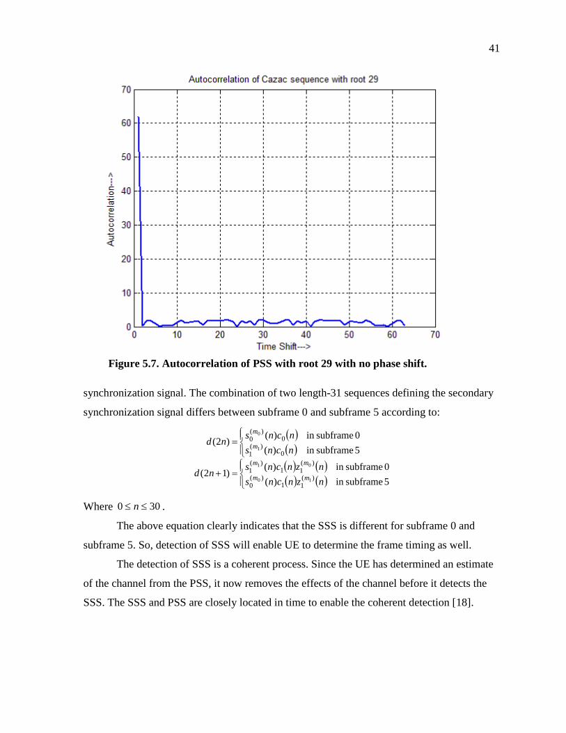
41
Figure 5.7. Autocorrelation of PSS with root 29 with no phase shift.
synchronization signal. The combination of two length-31 sequences defining the secondary
synchronization signal differs between subframe 0 and subframe 5 according to:
( )( )( ) ( )( ) ( )
=+
=
5 subframein )(0 subframein )()12(
5 subframein )(0 subframein )()2(
)(11
)(0
)(11
)(1
0)(
1
0)(
0
10
01
1
0
nzncnsnzncnsnd
ncnsncnsnd
mm
mm
m
m
Where 300 ≤≤ n .
The above equation clearly indicates that the SSS is different for subframe 0 and
subframe 5. So, detection of SSS will enable UE to determine the frame timing as well.
The detection of SSS is a coherent process. Since the UE has determined an estimate
of the channel from the PSS, it now removes the effects of the channel before it detects the
SSS. The SSS and PSS are closely located in time to enable the coherent detection [18].

42
Figure 5.8. Autocorrelation of PSS with root 34 with no phase shift.
Figure 5.9. Estimation of symbol start using cross and autocorrelation.
43
Figure 5.10. Determining the length of the symbol and this can be used to discard the cyclic prefix.
For our simulation, we began by assuming that the UE detected the PSS in subframe
0. So, the SSS is now,
where c0(n) and c1(n) are derived from the PSS.
The block diagram in Figure 5.17 assists in descrambling the SSS signal [19].
The following steps illustrate the detection of the SSS (The main goal is to determine
m0 and m1 so the UE can then use Table 5.2 and obtain the right cell identity). In our
simulation, say m0=25 and m1=26.
1. Channel effects are removed from the SSS and any frequency offset determined earlier is corrected.
2. The received signal is de-interleaved into the odd part and the even part, i.e. d(2n) and d(2n+1).Since N(2)
ID is known from the PSS, the scrambling code c0(n) is already
44
Figure 5.11. Auto-correlation of PSS sequence with itself with no offset.
known to the UE and can be descrambled from the received signal. So, has only one unknown m0 in s(m0)
0(n). It can be seen from Table 5.2 that both m0 and m1 have values between 0 and 30 only. So the UE now correlates the descrambled signal with 30 copies of s(m0)
0(n) to determine a match. Figure 5.18 shows the correlator output with the correct matching sequence for the even part s0 and Figure 5.19 shows the correlator output with incorrect matching sequence for s0.
We see that the peak for both is almost the same, but the peak for the sequence with correct match is at the beginning of the sequence and there is an offset for all other correlations. Now, the UE has determined m0 or m1, but since it does not know which subframe it is in, let us denote it by M. In our case, M is determined to be 25.
3. Now that the UE knows one value of m0 or m1, it can use it to descramble the sequence z, which is represented by, )31mod))8mod(((~)( 0
)(1
0 mnznz m += [Assuming we have detected m0].
45
Figure 5.12. Correlation between received signal and sequence with root 25 at UE.
4. Now, from this equation,
( )( )( ) ( )( ) ( )
=+
=
5 subframein )(0 subframein )()12(
5 subframein )(0 subframein )()2(
)(11
)(0
)(11
)(1
0)(
1
0)(
0
10
01
1
0
nzncnsnzncnsnd
ncnsncnsnd
mm
mm
m
m
5. Say, the UE is in subframe zero, c0 was known to the UE, m0 was determined using
s0(.) and using this m0 ,z1 was descrambled.
6. Now, c1 also can be descrambled using the known value of N(2)ID.
7. Now, s1 can be correlated with the 30 sequences at the receiver to obtain the right match and this gives m1. (denoted by M’).
8. But, since the receiver doesn’t know if it is in subframe 0 or subframe1, it uses the M and M’ from the above steps and detects the value of N(1)
ID from Table 5.2.
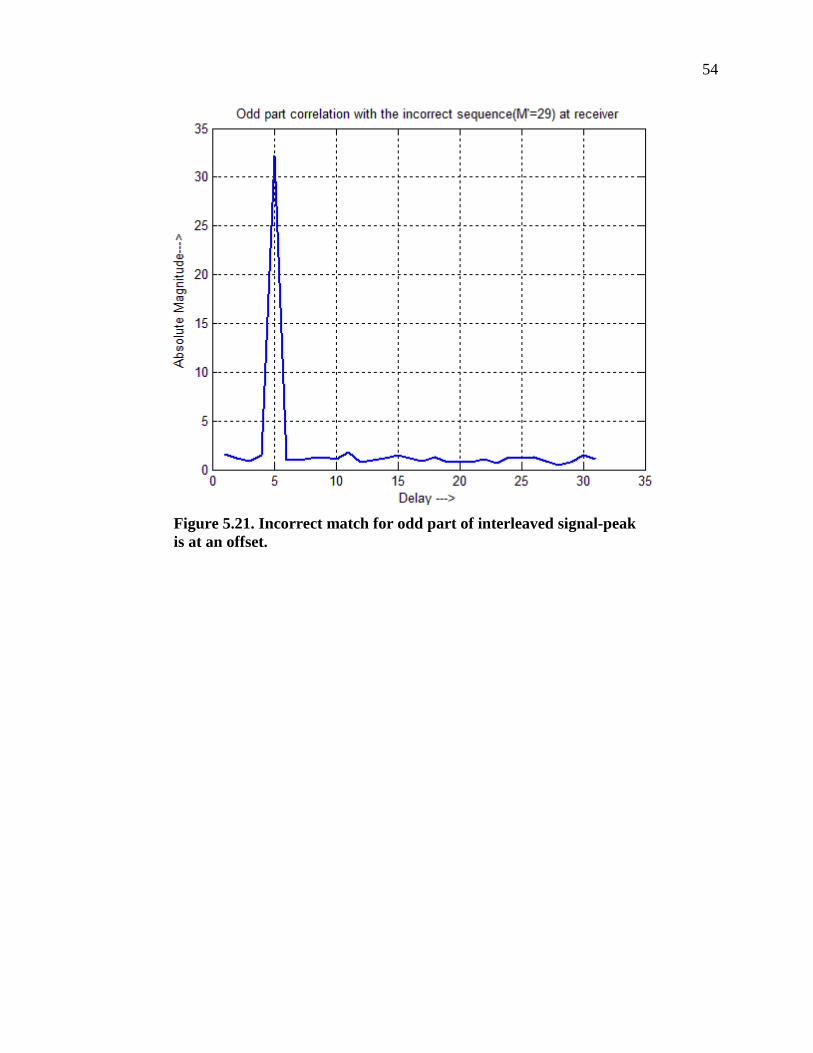
9. In our simulation m0=25 and m1=26. Figure 5.20 shows the correlator output for an exact match for the odd part of the signal s1and Figure 5.21 shows the output with a sequence that does not match the odd part of the transmitted sequence s1.
46
Figure 5.13. Correlation between received signal and sequence with root 29 at UE.
Now that we have M(25) and M’(26) and m0 is always less than m1, it can be
concluded that m0 < m1, m0=25 and m1=26.
From table 6.2 this corresponds to N(1)ID =25.
So, now the Cell Identity: NcellID = 3 N(1)
ID + N(2)ID
NcellID=3 X 25 + 0=75
With this the UE is also able to determine the subframe number, thus completing
frame timing synchronization also.
At the end of this step, the UE:
1. Has determined the radio cell ID.
2. Is synchronized in Time and Frequency with the radio cell.
3. Is ready to receive Downlink broadcast data from the radio cell.

47
Figure 5.14. Correlation between received signal and sequence with root 34 at UE.
48
Figure 5.15. Time domain representation of actual and estimated channel.
49
Figure 5.16. Frequency domain representation of actual and estimated channel.

50
Figure 5.17. SSS Detection block diagram.

51
Figure 5.18. Correct match of signal with correlator for the de-interleaved even part.

52
Figure 5.19. Incorrect match of signal with correlator for the de-interleaved even part.

53
Figure 5.20. Correct match for odd part of interleaved signal.
54
Figure 5.21. Incorrect match for odd part of interleaved signal-peak is at an offset.

55
CHAPTER 6
CONCLUSION AND FUTURE WORK
This master’s thesis has investigated, studied and simulated the Mobile cell search
and synchronization Procedure in LTE.
This research began with a study of SC-FDMA, which is a primary candidate for
uplink in LTE. Though it is much more complex than OFDMA but the low PAPR is the most
useful property of SC-FDMA and it compels us to use it as an uplink LTE systems.
In this thesis we have observed the data transfer from the mobile unit to the cell site
for two users using SC-FDMA- the channel estimation using CAZAC sequences and
subsequent demodulation at the receiver. In SC-FDMA system we used CAZAC sequence
for channel estimation. Channel estimation is important to mitigate the effect of channel
using an equalizer.
Using block diagrams we have studied the working of LTE cell search. We have
demonstrated the properties of Zadoff-Chu sequences whose correlation properties make it
an excellent choice for the primary synchronization signal. We also demonstrated the issues
of timing and frequency synchronization and also channel estimation and simulated
procedures to overcome these issues using Matlab model. This thesis gives the importance
of timing and frequency synchronization for successful demodulation of received data.

56
REFERENCES
[1] Google. (n.d.). LTE Encyclopedia [Online]. Available: https://sites.google.com/site/lteencyclopedia/home
[2] Wikipedia. (2011). 3GPP Long Term Evolution [Online]. Available: http://en.wikipedia.org/wiki/3GPP_Long_Term_Evolution
[3] Y. G. Li, and G. L. Stüber, Eds., Orthogonal Frequency Division Multiplexing for Wireless Communications. New York: Springer, 2006.
[4] R. Van Nee, and R. Prasad, OFDM for Wireless Multimedia Communications. Norwood, MA: Artech House Publishers, 2000
[5] National Instruments. (2006). Theory of Frequency Division Multiplexing [Online]. Available: http://zone.ni.com/devzone/cda/ph/p/id/269
[6] ProcessOnline. (2010). Applying wireless to EtherNet/IP automation systems — Part 1 [Online]. Available: http://www.processonline.com.au/articles/37629-Applying-wireless-to-EtherNet-IP-automation-systems-Part-1
[7] E. Lawrey. (2001). SkyDSP tutorial [Online]. Available: http://www.skydsp.com/publications/4thyrthesis/chapter1.htm
[8] B. Schrick, and M. J. Riezenman, “Wireless Broadband in a Box,” IEEE Spectrum, vol. 39, no. 6, pp. 38-43, June 2002.
[9] J. G. Andrews, A. Ghosh, and R. Muhamed, Fundamentals of WiMAX. New York: Prentice Hall.
[10] F. J. Harris, “Orthogonal frequency division multiplexing, OFDM,” presented at Department of Electrical Engineering, San Diego State University, San Diego, CA, 2008.
[11] Conniq. (2009). Introduction to FDM, OFDM, OFDMA, SC-FDMA [Online]. Available: http://www.conniq.com/WiMAX/fdm-ofdm-ofdma-sofdma-02.htm
[12] F. Khan, LTE for 4G Mobile Broadband. Cambridge, MA: Cambridge University Press, 2009.
[13] 3GPP. (n.d.). 3GPP TR 25.913 - v7.3.0, Requirements for EUTRA and EUTRAN [Online]. Available: http://www.3gpp.org/ftp/Specs/archive/25%5Fseries/25.913/
[14] European Telecommunications Standards Institute, 3GPP TS 36.211 version 9.1.0 Release 9, Sophia Antipolis, France: ETSI, 2010.
[15] H. G.Myung, J. Lim, and D. J. Goodman, “Single Carrier FDMA forUplink Wireless Transmission,” IEEE Veh. Technol. Soc., vol. 1, no. 3, pp. 30-38, Sept. 2006.
[16] A. Roessler, Cell Search and Cell Selection in UMTS LTE. Munich, Germany: Rhode and Schwarz, 2009.

57
[17] Wikipedia. (2011). Zadoff–Chu Sequence [Online]. Available: http://en.wikipedia.org/wiki/Zadoff%E2%80%93Chu_sequence
[18] H.-G. Park, I.-K. Kim, and Y.-S. Kim, “Efficient coherent neighbor cell search for synchronous 3GPP LTE system,” Electron. Lett., vol.44, no.21, Oct. 2008.
[19] J.-I. Kim, J.-S. Han, H.-J. Roh, and H.-J. Choi, “SSS detection method for initial cell search in 3GPP LTE FDD/TDD dual mode receiver,” presented at the 9th Int. Symp. on Communications and Information Technology, Incheon, Korea, Sept. 2009.
58
APPENDIX
SAMPLE MATLAB CODE
59
---------------------------------SYMBOL BOUNDARY DETECTION------------------------------- % Initialize the roots of the Zadoff-Chu Sequence u=25; u1=29; u2=34; % Initialize variables for the sequence. d=zeros(1,64); d1=zeros(1,64); d2=zeros(1,64); % Generate the sequences with three roots. for n=0:62 d(n+1)=exp(-j*(pi*u*n*(n+1))/63); d1(n+1)=exp(-j*(pi*u1*n*(n+1))/63); d2(n+1)=exp(-j*(pi*u2*n*(n+1))/63); end % Zero puncture the center element. d(32)=0; d1(32)=0; d2(32)=0; transmitted_sec_signal_1=ifft(d); SCFDMA.channel=[1 0 0 0 0.1 0 0 0 j*0.1 0 -0.05]; transmitted_sec_signal_2=[transmitted_sec_signal_1(49:64) transmitted_sec_signal_1 transmitted_sec_signal_1(49:64) transmitted_sec_signal_1]; transmitted_sec_signal_3=filter(SCFDMA.channel,1,transmitted_sec_signal_2); transmitted_sec_signal=transmitted_sec_signal_3.*exp(j*2*pi*(0:length(transmitted_sec_signal_3)-1)*(1/63)); % Estimate the frame start delay_line=zeros(1,65); delay_len=64; autocor_set=zeros(1,64); croscor_set=zeros(1,64); for nn=1:length(transmitted_sec_signal) delay_line=[transmitted_sec_signal(nn) delay_line(1:64)]; autocor(nn)=delay_line(65)*conj(delay_line(65)); croscor(nn)=delay_line(1)*conj(delay_line(65)); % autocor and croscor in sets of 64 autocor_set=[autocor(nn) autocor_set(1:63)];

60
croscor_set=[croscor(nn) croscor_set(1:63)]; % Running average over 64 samples. autocor_sum(nn)=sum(autocor_set); croscor_sum(nn)=sum(croscor_set); preamble_start_detection(nn)=croscor_sum(nn)/(autocor_sum(nn)+00000.1); end for q=1:100 if abs(preamble_start_detection(q)) > 0.5 frame_start=q; break; end end figure(1); plot(abs(preamble_start_detection)); grid on; -----------------------------PRIMARY SYNCHRONIZATION SIGNAL---------------------------- % Take IFFT of this signal as part of OFDM transmitter ofdm_transmitted_3=ifft(d); % Add cyclic prefix ofdm_transmitted_2=[ofdm_transmitted_3(49:64) ofdm_transmitted_3]; % Initialize the channel SCFDMA.channel=[1 0 0 0 0.1 0 0 0 j*0.1 0 -0.05]; % Filter the signal through the channel ofdm_transmitted_1=filter(SCFDMA.channel,1,ofdm_transmitted_2); % Add a spin ofdm_transmitted_4=ofdm_transmitted_1.*exp(j*2*pi*(0:length(ofdm_transmitted_1)-1)*(1/63)); % Received signal with spin for purposes of detecting the frequency offset. ofdm_transmitted=ofdm_transmitted_4(17:80); % Take fft as part of OFDM receiver. ofdm_received=fft(ofdm_transmitted); % FFT of reference signal copies at receiver. fft_op=fft(d); fft_op1=fft(d1);

61
fft_op2=fft(d2); fft_op_rotated=fft(ofdm_received); % Consider original sequence as the sequence with root 25. % Cross correlation of this rotated sequence with the sequence with root 29. conj_prod_cross1=fft_op_rotated.*conj(fft_op1); figure(1); ifft_op_cross1=ifft(conj_prod_cross1); plot(abs(fftshift(ifft_op_cross1))); grid on; title('PSS - Cross Correlation of OFDM transmitted Cazac sequence with root 25 and root 29'); xlabel('Delay--->'); ylabel('Absolute Magnitude--->') axis([0 64 0 70]) % Cross correlation of this sequence with the sequence with root 34. conj_prod_cross2=fft_op_rotated.*conj(fft_op2); figure(2); ifft_op_cross2=ifft(conj_prod_cross2); plot(abs(fftshift(ifft_op_cross2))); grid on; title('PSS - Cross Correlation of OFDM transmitted Cazac sequence with root 25 and root 34'); xlabel('Delay--->'); ylabel('Absolute Magnitude--->'); axis([0 64 0 70]) % Cross correlation of this sequence with the sequence with root 25 conj_prod_cross3=fft_op_rotated.*conj(fft_op); figure(3); ifft_op_cross3=ifft(conj_prod_cross3); plot(abs((ifft_op_cross3))); grid on; title('Cross Corr of transmitted Cazac sequence with root 25 and root 25 with 15KHz offset'); xlabel('Delay--->'); ylabel('Absolute Magnitude--->')

62
figure(4); plot(abs(d)); title('Magnitude of PSS - It is a CAZAC sequence with DC punctured'); xlabel('Sample--->'); ylabel('Absolute Magnitude--->') axis([0 70 0 2]); grid on; ------------------------------------------SSS GENERATION -------------------------------------------- % Secondary Synchronization Signal is an interleaved concatenation of two % length 31 sequences % d(2n)= s0m0(n)c0(n) % d (2n+1) = s1m1(n)c1(n)z1m0(n); in subframe 0 % d(2n)=s1m1(n)c0(n) % d(2n+1)=s0m0(n)c1(n)z1m1(n); in subframe 5 % where 0<=n<=30 % for our case, say N1=25, mo=25, m1=26 (m0 and m1 can be got from the % table) % Say, N2=0, as obtained from primary synch signal clear all; Signal_rotated_ofdm_channel_64point; Receiver_Match_Signals; %SSS_generation; N2=0; m0=25; m1=26; % Generate signals z1m0 and z1m1 xz(1)=0; xz(2)=0; xz(3)=0; xz(4)=0; xz(5)=1; for i=1:26 xz(i+5)=mod((xz(i+4)+xz(i+2)+xz(i+1)+xz(i)),2); end for n=1:31 zbar(n)=1-(2*xz(n)); end for nn=1:2:61 z1m0(nn)=zbar((mod((nn+mod(m0,8)),31))+1); z1m1(nn)=zbar((mod((nn+mod(m1,8)),31))+1); end % Generate the signals c0(n) and c1(n) xc(1)=0; xc(2)=0; xc(3)=0; xc(4)=0;xc(5)=1; for ii=1:26
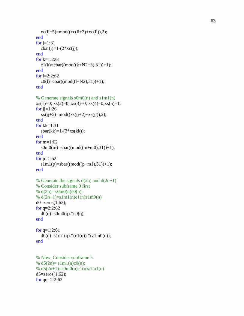
63
xc(ii+5)=mod((xc(ii+3)+xc(ii)),2); end for j=1:31 cbar(j)=1-(2*xc(j)); end for k=1:2:61 c1(k)=cbar((mod((k+N2+3),31))+1); end for l=2:2:62 c0(l)=cbar((mod((l+N2),31))+1); end % Generate signals s0m0(n) and s1m1(n) xs(1)=0; xs(2)=0; xs(3)=0; xs(4)=0;xs(5)=1; for jj=1:26 xs(jj+5)=mod((xs(jj+2)+xs(jj)),2); end for kk=1:31 sbar(kk)=1-(2*xs(kk)); end for m=1:62 s0m0(m)=sbar((mod((m+m0),31))+1); end for p=1:62 s1m1(p)=sbar((mod((p+m1),31))+1); end % Generate the signals d(2n) and d(2n+1) % Consider subframe 0 first % d(2n)= s0m0(n)c0(n); % d(2n+1)=s1m1(n)c1(n)z1m0(n) d0=zeros(1,62); for q=2:2:62 d0(q)=s0m0(q).*c0(q); end for q=1:2:61 d0(q)=s1m1(q).*(c1(q)).*(z1m0(q)); end % Now, Consider subframe 5 % d5(2n)= s1m1(n)c0(n); % d5(2n+1)=s0m0(n)c1(n)z1m1(n) d5=zeros(1,62); for qq=2:2:62

64
d5(qq)=s1m1(qq).*c0(qq); end for qq=1:2:61 d5(qq)=s0m0(qq).*(c1(qq)).*(z1m1(qq)); end