MMIICCRROOWWAAVVEESS – #4466221166 · Department of Electrical Engineering Technion – Israel...
323
Department of Electrical Engineering Technion – Israel Institute of Technology M M M I I I C C C R R R O O O W W W A A A V V V E E E S S S – – – # # # 4 4 4 6 6 6 2 2 2 1 1 1 6 6 6 L L L E E E C C C T T T U U U R R R E E E N N N O O O T T T E E E S S S based upon lectures delivered by Prof. L. Schächter M M M a a a r r r c c c h h h 2 2 2 0 0 0 0 0 0 9 9 9
Transcript of MMIICCRROOWWAAVVEESS – #4466221166 · Department of Electrical Engineering Technion – Israel...

Department of Electrical Engineering
Technion – Israel Institute of Technology
MMMIIICCCRRROOOWWWAAAVVVEEESSS ––– ###444666222111666
LLLEEECCCTTTUUURRREEE NNNOOOTTTEEESSS
based upon lectures delivered by
Prof. L. Schächter
MMMaaarrrccchhh 222000000999

This work is subject to copyright. All rights reserved, whether the whole part or part of the material is concerned, specifically the rights of translation, reprinting, reuse of illustrations, recitation, broadcasting, reproduction on microfilm, or in any other way, and storage in data banks and electronic storage. Duplication of this publication or parts thereof is permitted only with the explicit written permission of the authors. Violations are liable for prosecution.
i
CONTENTS
1 Transmission Lines 1
1.1 Simple Model ………………………………………………………… 2
1.2 Coaxial Transmission Line …………………………………………… 7
1.3 Low Loss System ……………………………………………………… 11
1.4 Generalization of the Transmission Line Equations ………………… 13
1.5 Non-Homogeneous Transmission Line ……………………………… 21
1.6 Coupled Transmission Lines ………………………………………… 24
1.7 Microstrip ……………………………………………………………… 26
1.8 Stripline ……………………………………………………………… 38
1.9 Resonator Based on Transmission Line ……………………………… 46
1.9.1 Short Recapitulation ………………………………………… 46
1.9.2 Short-Circuited Line ………………………………………… 50
1.9.3 Open-Circuited Line ………………………………………… 52
1.10 Pulse Propagation ……………………………………………………… 53
1.10.1 Semi-Infinite Structure ……………………………………… 53
1.10.2 Propagation and Reflection ………………………………… 59

ii
1.11 Appendix ……………………………………………………………… 64
1.11.1 Solution to Exercise 1.10 ……………………………………… 64
1.11.2 Solution to Exercise 1.11 ……………………………………… 65
1.11.3 Solution to Exercise 1.15 ……………………………………… 66
1.11.4 Solution to Exercise 1.17 ……………………………………… 68
2 Waveguides – Fundamentals 71
2.1 General Formulation …………………………………………………… 71
2.2 Transverse Magnetic (TM) Mode [Hz = 0] …………………………… 79
2.3 Transverse Electric (TE) Mode [Ez = 0] ……………………………… 82
2.4 Power Considerations ………………………………………………… 85
2.4.1 Power Flow …………………………………………………… 85
2.4.2 Ohm Loss ……………………………………………………… 88
2.4.3 Dielectric Loss ………………………………………………… 90
2.5 Mode Comparison …………………………………………………… 93
2.6 Cylindrical Waveguide ………………………………………………… 95
2.6.1 Transverse Magnetic (TM) Mode [Hz = 0] …………………… 95
2.6.2 Transverse Electric (TE) Mode [Ez = 0] ……………………… 97
2.6.3 Power Considerations ………………………………………… 100

iii
2.6.4 Ohm Loss ……………………………………………………… 104
2.7 Pulse Propagation ……………………………………………………… 107
2.8 Waveguide Modes in Coaxial Line …………………………………… 113
3 Waveguides – Advanced Topics 114
3.1 Hybrid Modes ………………………………………………………… 115
3.2 Dielectric Loading – TM01 …………………………………………… 125
3.3 Cross-Section Variation and Mode Coupling ………………………… 130
3.3.1 Step Transition – TE mode …………………………………… 130
3.3.2 Step Transition – TM0n Mode in Cylindrical Waveguide …… 139
3.4 Reactive Elements …………………………………………………… 146
3.4.1 Inductive Post ………………………………………………… 146
3.4.2 Diaphragm …………………………………………………… 153
3.5 Excitation of Waveguides ……………………………………………… 157
3.6 Coupling between Waveguides by Small Apertures ………………… 164
3.7 Surface Waveguides …………………………………………………… 165
3.7.1 Dielectric Layer above a Metallic Surface …………………… 166
3.7.2 Surface Waves along a Dielectric Fiber ……………………… 176
3.8 Transients in Waveguides ……………………………………………… 181

iv
3.9 Waveguide Based Cavities …………………………………………… 185
3.9.1 Power and Energy Considerations …………………………… 185
3.9.2 Rectangular Waveguide Cavity ……………………………… 187
3.9.3 Cylindrical Resonator ……………………………………… 191
3.9.4 Open Resonator – Rectangular Geometry (TM - Mode) ……… 193
3.9.5 Exciting a Cavity ……………………………………………… 194
3.10 Wedge in a Waveguide ……………………………………………… 197
3.10.1 Metallic Wedge ……………………………………………… 197
3.10.2 Dielectric Wedge ……………………………………………… 204
3.11 Appendix ……………………………………………………………… 207
3.11.1 Solution to Exercise 3.8 ……………………………………… 207
4 Matrix Formulations 211
4.1 Impedance Matrix …………………………………………………… 211
4.2 Scattering Matrix ……………………………………………………… 215
4.3 Transmission Matrix …………………………………………………… 220
4.4 Wave-Amplitude Transmission Matrix ……………………………… 221
4.5 Loss Matrix …………………………………………………………… 223
4.6 Directional Coupler …………………………………………………… 224

v
4.7 Coupling Concepts …………………………………………………… 225
4.7.1 Double Strip Line: Parameters of the Line …………………… 225
4.7.2 Equations of the System ……………………………………… 230
4.7.3 Simple Coupling Process ……………………………………… 233
5 Nonlinear Components 237
5.1 Transmission Line with Resistive Nonlinear Load …………………… 237
6 Periodic Structures 241
6.1 The Floquet Theorem ………………………………………………… 242
6.2 Closed Periodic Structure ……………………………………………… 252
6.2.1 Dispersion Relation …………………………………………… 254
6.2.2 Modes in the Groove …………………………………………… 259
6.2.3 Spatial Harmonics Coupling …………………………………… 261
6.3 Open Periodic Structure ……………………………………………… 264
6.3.1 Dispersion Relation …………………………………………… 266
6.4 Transients ……………………………………………………………… 271

vi
7 Generation of Radiation 276
7.1 Single-Particle Interaction …………………………………………… 277
7.1.1 Infinite Length of Interaction ………………………………… 277
7.1.2 Finite Length of Interaction …………………………………… 280
7.1.3 Finite Length Pulse …………………………………………… 281
7.1.4 Cerenkov Interaction ………………………………………… 282
7.1.5 Compton Scattering: Static Fields …………………………… 284
7.1.6 Compton Scattering: Dynamic Fields ………………………… 285
7.1.7 Uniform Magnetic Field ……………………………………… 286
7.1.8 Synchronism Condition ……………………………………… 287
7.2 Radiation Sources: Brief Overview …………………………………… 290
7.2.1 The Klystron ………………………………………………… 290
7.2.2 The Traveling Wave Tube ……………………………………… 291
7.2.3 The Gyrotron ………………………………………………… 293
7.2.4 The Free Electron Laser ……………………………………… 295
7.2.5 The Magnetron ………………………………………………… 297
7.3 Generation of radiation in a waveguide ……………………………… 299
7.4 Generation of radiation in a cavity …………………………………… 308

Chapter 1: Transmission Lines
In this chapter we shall first recapitulate some of the topics learned in the
framework of the course ``Waves and Distributed Systems'' and then we shall
extend the analysis to topics that are of
importance to microwave devices. But first a
few examples:
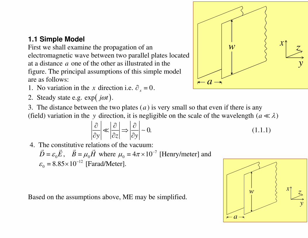
1.1 Simple Model First we shall examine the propagation of an
electromagnetic wave between two parallel plates located
at a distance a one of the other as illustrated in the
figure. The principal assumptions of this simple model
are as follows:
1. No variation in the x direction i.e. = 0x∂ .
2. Steady state e.g. ( )exp j tω .
3. The distance between the two plates (a ) is very small so that even if there is any
(field) variation in the y direction, it is negligible on the scale of the wavelength ( )λa
0.y z y
∂ ∂ ∂⇒
∂ ∂ ∂ ∼ (1.1.1)
4. The constitutive relations of the vacuum:
0 0= , =ε µ D E B H where
7
0 = 4 10µ π −× [Henry/meter] and
12
0 = 8.85 10ε −× [Farad/Meter].
Based on the assumptions above, ME may be simplified.
a
y
xzw
a
y
xzw
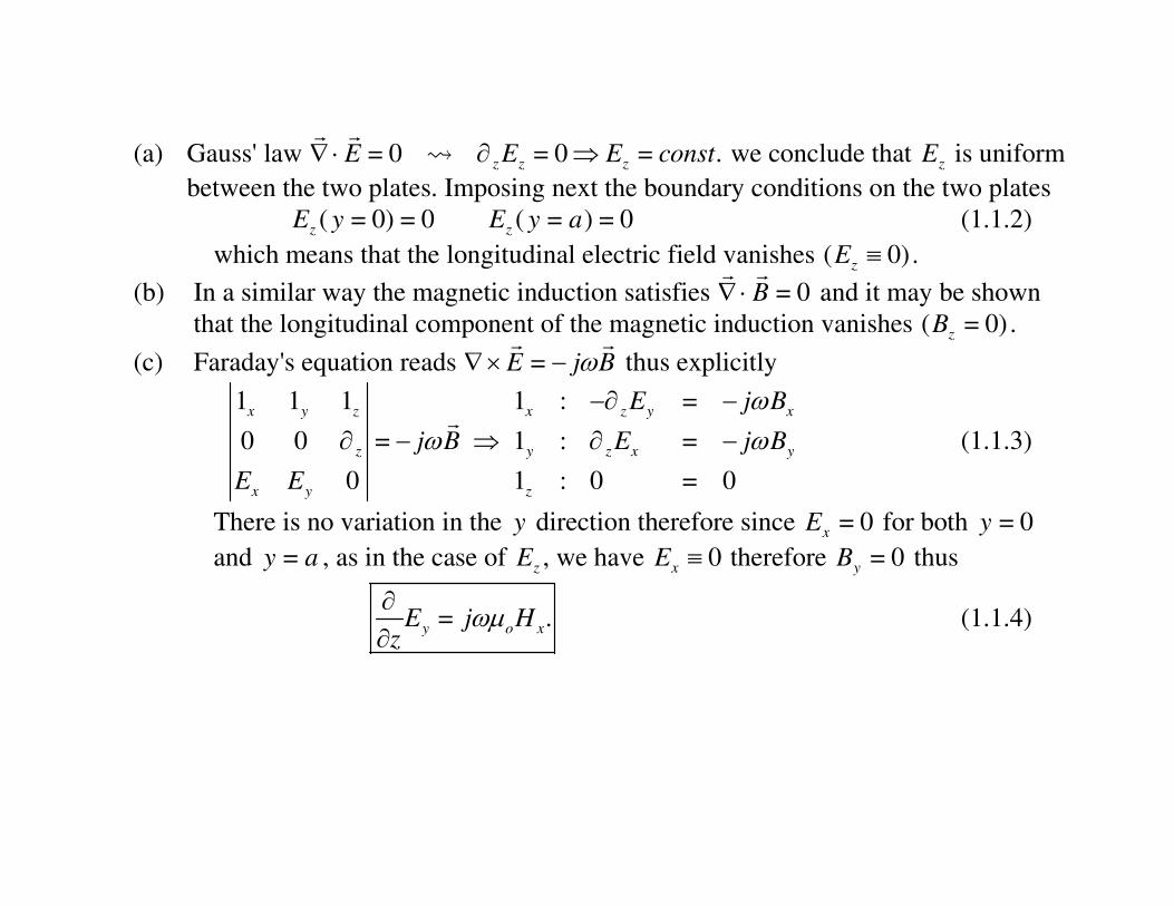
(a) Gauss' law = 0 = 0 = .z z zE E E const∇ ⋅ ∂ ⇒
we conclude that zE is uniform
between the two plates. Imposing next the boundary conditions on the two plates
( = 0) = 0 ( = ) = 0z zE y E y a (1.1.2)
which means that the longitudinal electric field vanishes ( 0)≡zE .
(b) In a similar way the magnetic induction satisfies = 0∇⋅
B and it may be shown
that the longitudinal component of the magnetic induction vanishes ( = 0)zB .
(c) Faraday's equation reads = ω∇ × − E j B thus explicitly
1 1 1 1 : =
0 0 = 1 : =
0 1 : 0 = 0
x y z x z y x
z y z x y
x y z
E j B
j B E j B
E E
ωω ω
−∂ −
∂ − ⇒ ∂ −
(1.1.3)
There is no variation in the y direction therefore since = 0xE for both = 0y
and =y a , as in the case of zE , we have 0≡xE therefore = 0yB thus
= .y o x
E j Hz
ωµ∂∂
(1.1.4)

(d) Ampere's law reads = ω∇ ×
H j D , or explicitly taking
advantage of the vanishing components we get
1 : 0 = 01 1 1
0 0 = 1 : =
0 0 1 : 0 = 0
xx y z
z y z x y
x z
j D H j D
H
ω ω∂ ⇒ ∂
(1.1.5)
hence
= .x o y
H j Ez
ωε∂∂
(1.1.6)
From these two equations [(1.1.4) and (1.1.6)] it can be readily seen that we obtain the
wave-equation for each one of the components:
2 2
2 2
=
= 0
=
x o y
y
y o x
H j Ez
Ez c
E j Hz
ωεω
ωµ
∂ ∂∂ ⇒ + ∂ ∂ ∂
(1.1.7)
which has a solution of the form
= exp expyE A j z B j zc c
ω ω − +
(1.1.8)
a
y
xzw

It is convenient at this point to introduce the notation in terms of
voltage and current. The voltage can be defined since = 0⋅∫E d ; it
reads
( ) = ( ) .− yV z E z a (1.1.9)
In order to define the current we recall that based on the boundary conditions we have
1 2( ) =× −
n H H K where K is the surface current. Consequently, denoting by w the
height of the metallic plates, the local current is = zI K w or
( ) = ( ) .xI z H z w (1.1.10)
Based on these two equations [(1.1.9)–(1.1.10)] it is possible to write
y o x o o
x o y o o
V I aE j H j V j I
z z a w z w
I V wH j E j I j V
z z w a z a
ωµ ωµ ω µ
ωε ωε ω ε
∂ ∂ ∂ = ⇒ − = ⇒ = − ∂ ∂ ∂ ∂ ∂ ∂ = ⇒ = − ⇒ = − ∂ ∂ ∂
(1.1.11)
The right hand side in both lines of (1.1.11) represent the so-called transmission line
equation also known as telegraph equations.
a
y
xzw

( )
( )
( )
( )
dV z j I z
dz
d
L
I z j V zz
Cd
ω
ω
= −
= − (1.1.12)
C being the capacitance per unit length whereas L is the inductance per unit length;
ando o
a wL C
w aµ ε= = . As expected, these two equations lead also to the wave equation
22
2= ( ) ( ) = 0
= ( )
dV dj LI z V zdz dzdI
j CV z LCdz ω
ω β
ω β
− + =
−
(1.1.13)
The general solution is ( ) =β β− +j z j z
V z Ae Be and correspondingly, the expression for
the current is given by
1
( ) = =dV j z j z
I z Ae Bej L dz L
β β βω ω− − −
(1.1.14)
defining the characteristic impedance 1 = =β ω
ω ω−c
LCZ
L L or ,c
LZ
C≡ we get
a
y
xzw

1
( ) = [ ].β β− +−
c
j z j zI z Ae Be
Z (1.1.15)
In the specific case under consideration
= = , = = .o
c o
o
a
awZ LCw w c
a
µ ωη β ω
ε (1.1.16)
1.2 Coaxial Transmission Line
As indicated in the previous case, two parameters are
to be determined: the capacitance per unit length ( )C
and the inductance per unit length ( )L . According to
(1.1.11) these two parameters can be determined in
static conditions. We determine next the capacitance
per unit length of a coaxial structure. For this
purpose it is assumed that on the inner wire a voltage
oV is applied, whereas the outer cylinder is grounded.
2Rint
2Rext

Consequently, the potential is given by
ln( / )
( ) = .ln( / )
ϕ exto
int ext
r Rr V
R R (1.2.1)
and the corresponding electric field associated with this potential is
1 1
= = .ln( / )
ϕ∂− −
∂r o
int ext
E Vr r R R
(1.2.2)
The charge per unit surface at = extr R is calculated based on 1 2( ) = ρ⋅ −
sn D D and it is
given by
( )
00
1= .
ln /ρ εs
ext ext int
V
R R R (1.2.3)
Based on this result, the charge per unit length ( )∆ z may be expressed as
( )0
21= 2 = 2 = .
ln /ln
o o os ext ext
z ext ext intext
int
V VQR R
R R RR
R
ε πρ π ε π
∆
(1.2.4)
Consequently, the capacitance per unit length is given by

2/
= .ln( / )
oz
o ext int
QC
V R R
πε∆≡ (1.2.5)
In a similar way, we shall calculate the inductance per unit length. Assuming that
the inner wire carries a current I , based on Ampere law the azimuthal magnetic field is
( ) = .2
φ πoI
H rr
(1.2.6)
With this expression for the magnetic field, we can calculate the magnetic flux. It is given
by
= ( ) = ln .2
Rext ext
o z o zR
int int
RIdrH r
Rφµ µ
πΦ ∆ ∆∫ (1.2.7)
The inductance per unit length ∆ z is
/
= ln .2
o extz
int
RL
I R
µπ
Φ ∆≡
(1.2.8)
o
∆ z
I

To summarize the parameters of a coaxial transmission line
1= ln
2
extc o
int
RLZ
C R
c
ηπ
ωβ
=
=
(1.2.9)
Exercise 1.1: Determine cZ and β for a coaxial line filled with a material ( ,ε µr r )?

1.3 Low Loss System
Based on Ampere's law we obtained
= ( ) = ( ),ωε ε ω∇ × −
o
dH j E I z j CV z
dz
(1.3.1)
where we assumed a line without dielectric (ε r ) and Ohm ( )σ loss. In the case of
dielectric loss we have
=ε ε ε′ ′′−r j (1.3.2)
or in our case
.j C j C G Yω ω→ + ≡ (1.3.3)
In a similar way based on Faraday's law
= ( ) = ( )o r
dE j H V z j LI z
dzωµ µ ω∇× − ⇒ −
(1.3.4)
and the magnetic losses
=µ µ µ′ ′′−r r rj
allows us to extend the definition according to
ω ω + ≡j L j L R Z (1.3.5)
hence the equations
a
y
xzw

( ) = ( )
( ) = ( )
dI z YV z
dz
dV z ZI z
dz
−
− (1.3.6)
may be conceived as a generalization of the transmission line equations in the presence of
loss. The characteristic impedance for small loss line is
= 12 2ω ω
+ − c
Z L G RZ j
Y C C L (1.3.7)
and the wave number
2 2
2 2 2 2 2
=
2 2
14 8 8
o
o
j
GZR
Z
RG G RLC
LC C L
γ α β
α
β ωω ω ω
+
+
− + +
(1.3.8)
Exercise 1.2: Prove the relations in Eq. (1.3.8).
a
y
xzw

1.4 Generalization of the Transmission Line Equations
The fundamental assumptions of the analysis are:
(i) TEM, (ii) the wave propagates in the z direction, (iii) we distinguish between
longitudinal ( z ) and transverse (⊥ ) components = 1⊥
∂∇ ∇ +
∂
zz
.
From Faraday law, = ωµ µ∇ × −
o rE j H , we obtain
1 ( )1 1 1
= 1
0 1
− ∂
∂ ∂ ∂ ∂
∂ − ∂
x z yx y z
x y z y z x
x y z x y y x
E
E
E E E E
(1.4.1)
thus
1 : =1 : 1 =
1 : =
1 : = 0 1 : = 0.
ωµ µωµ µ
ωµ µ⊥
⊥ ⊥
⊥ ⊥
−∂ − ∂× −
+∂ − ∂∂ − ∂ ∇ ×
x z y o r x
z o r
y z x o r y
z x y y x z
E j H Ej H
E j H z
E E E
(1.4.2)

In a similar way, from Ampere's law we have
1 : 1 ==
1 : = 0.
ωε εωε ε
⊥⊥ ⊥
⊥ ⊥
∂×
∇ × + ⇒ ∂ ∇ ×
z o r
o r
z
Hj E
H j E z
H
(1.4.3)
From the two curl equations 2
2
= 0 = ( ) ( , ) = 0
= 0 = ( ) ( , ) = 0,
ϕ ϕ
ψ ψ⊥ ⊥ ⊥ ⊥ ⊥
⊥ ⊥ ⊥ ⊥ ⊥
∇ × ⇒ ∇ ⇒ ∇
∇ × ⇒ ∇ ⇒ ∇
E E g z x y
H H h z x y (1.4.4)
we conclude that the transverse variations of the transverse field components are
determined by 2D Laplace equation justifying the use of DC quantities adopted above
(capacitance and inductance per unit length). From the other two equations we get the
wave equation
2
2
1
1 1 1 = [ ],
z o r
z z o r z o r o r
E Hj
z z z
E Hj j j E
z z
ωµ µ
ωµ µ ωµ µ ωε ε
⊥ ⊥
⊥ ⊥⊥
∂ ∂ ∂× = − ∂ ∂ ∂
∂ ∂× × = − × − ∂ ∂
(1.4.5)
or explicitly

2 2
2 2= 0.r r E
z c
ωµ ε ⊥
∂+ ∂
(1.4.6)
The last equation determines the dynamics of ( )g z [see (1.4.4)] and
the solution has the form ( ) =β− j z
g z e where = ( / )β ω ε µr rc . Note that
1 1
1 1
o rz o r z
o r
o rz o r z
o r
Ej H E H
z
Hj E H E
z
µ µωµ µ
ε ε
ε εωε ε
µ µ
⊥⊥ ⊥ ⊥
⊥⊥ ⊥ ⊥
∂× = − ⇒ × =
∂
∂× = ⇒ × = −
∂
(1.4.7)

As in the previous two cases we shall see next how
the electric parameters can be calculated in the
general case and for the sake of simplicity we shall
assume that the medium has uniform transverse and
longitudinal properties. The electric field in the entire space is given by
= ( )βϕ⊥ ⊥
−− ∇ j zE e whereas the magnetic field is
= ( 1 ) .ε ε βϕµ µ⊥ ⊥
−− ×∇
o rz
o r
j zH e (1.4.8)
Note that associated to this electric field, one can define the voltage
2 2 2
1 1 1
= = =ϕ ϕ⊥ ⊥− ⋅ ∇ ⋅∫ ∫ ∫
s s s
os s s
V E d d d (1.4.9)
such that ( ) =β−
o
j zV z V e . On the two (ideal) conductors the electric field generates a
surface charge given by
= ,ρ ε ε ⊥⋅
s o rn E (1.4.10)
therefore the charge per unit length is
= = ( ).ρ ε ε ⊥⋅∆ ∫ ∫
s o r
z
Qdl dl n E (1.4.11)
Since by virtue of linearity of Maxwell's equations
1
2
V
0=Vx
y
z
0V=s
s

the charge per unit length is proportional to the applied
voltage 0=∆ z
QCV we get
0
1= ( ).ε ε ⊥⋅∫
o rC d n E
V (1.4.12)
In a similar way, the magnetic field generates on the metallic electrode (wire) a surface
current given by
= .⊥×
sJ n H (1.4.13)
Since it was shown that = 1ε εµ µ⊥ ⊥×
o r
z
o r
H E we conclude that
= [1 ] ( )1o r o rs z z
o r o r
J n H n E n Eε ε ε εµ µ µ µ⊥ ⊥ ⊥= × × × = ⋅
(1.4.14)
hence the total current is
( )0 1 o rs z
o r
I J dl dl n Eε εµ µ ⊥= ⋅ = ⋅∫ ∫
(1.4.15)
At this point rather than calculating the inductance per unit length we combine the
previous result for the charge per unit length and (1.4.15) the result being
1
2
V
0=Vx
y
z
0V=s
s

= = ./
o r
o ro
z r ro r
dl n EI c
Q dl n E
ε εµ µ
µ εε ε
⊥
⊥
⋅
∆ ⋅
∫
∫
(1.4.16)
However, having established this relation between the current and the charge per unit
length we may use again the linearity of Maxwell's equations and express 0/ =∆ zQ CV .
Substituting in Eq. (1.4.16) we get
0 =µ εo r r
I c
CV (1.4.17)
but by definition
0
0
= ,c
VZ
I (1.4.18)
which finally implies that
1
= .µ εc r r
c
CZ
This result leads to a very important conclusion namely, in a transmission line of
uniform electromagnetic properties it is sufficient to calculate the capacitance per
unit length. Bearing in mind that = /cZ L C we find that once C is established,
1
2
V
0=Vx
y
z
0V=s
s

2= .
µ εr rLCc
(1.4.19)
It is important to re-emphasize that this relation is valid only if the electromagnetic
properties ( , )ε µr r are uniform over the cross-section.
Exercise 1.3: Calculate the capacitance per unit length of two wires of radius R which
are at a distance > 2d R apart.
Another quantity that warrants consideration is the average power
( ) ( )
* *
* *
1 1= R 1 = R 1 1
2 2
1 2 1= R
2 4
2= = [ ].
o rz z z
o r
o r o ro r
o r o r o r
e e m
o o r r r r
P e dxdy E H e dxdy E E
e dxdy E E dxdy E E
cW W W
ε εµ µ
ε ε ε εε ε
µ µ ε ε µ µ
ε µ ε µ ε µ
⊥ ⊥ ⊥ ⊥
⊥ ⊥ ⊥ ⊥
× ⋅ × × ⋅
⋅ = ⋅
+
∫ ∫
∫ ∫
(1.4.20)
1
2
V
0=Vx
y
z
0V=s
s

Exercise 1.4: In the last expression we used the fact that =e mW W -- prove it.
Exercise 1.5: Show that the power can be expressed as 2 *1 1
= | | =2 2
c o o oP Z I V I .
Finally, we may define the energy velocity as the average power propagating along the
transmission line over the total average energy per unit length
en = = .µ ε+e m r r
P cV
W W
Exercise 1.6: Show that the material is not frequency dependent, this quantity equals
exactly the group velocity. What if not? Namely r ( )ε ω .

1.5 Non-Homogeneous Transmission Line
There are cases when either the electromagnetic properties or the
geometry vary along the structure. In these cases the impedance per unit
length ( )Z and admittance ( )Y per unit length are z -dependent i.e.
( )( ) ( )
( )( ) ( ).
dV zZ z I z
dz
dI zY z V z
dz
= −
= − (1.5.1)
As a result, the voltage or current satisfy an equation that to some extent differs from the
regular wave equation
[ ]
2
2
( ) ( )( ) ( )
ln ( ) ( ) ( ) ( )
d V dZ z dI zI z Z z
dz dz dz
d dVZ z Z z Y z V z
dz dz
= − −
= +
(1.5.2)
A solution of a general character is possible only using
numerical methods. However, an analytic solution is
possible if we assume an ``exponential'' behavior of the

form
( )
( ) ( )( ) exp
exp
o
o
Z z j L qz
Y z j C qz
ω
ω
=
= − (1.5.3)
Substituting these expressions in Eq. (1.5.2) we get
2
2
2
( )= 0ω− + o o
d V z dVq L C V
dz dz (1.5.4)
therefore assuming a solution of the form 1( ) =γ− z
oV z V e we conclude that
2 2
1
1= 4 .
2γ ω − ± −
o oq q L C (1.5.5)
In a similar way, the equation for the current is given by
2
2ln[ ( )] ( ) = 0.− −
d I dI dY z YZI z
dz dz dz (1.5.6)
Assuming a solution of the form 2=γ− z
oI I e we obtain
2 2
2
1= 4 .
2γ ω ± −
o oq q L C (1.5.7)
It is convenient to define
2
2
2 2
/ 4,ω ≡c
o o
q
L C (1.5.8)

which sets a ``cut-off'' in the sense that for <ω ωc both 1γ and 1γ are real.
The second important result is that the impedance along the transmission
line
1
2
( )= = (0)
( )
γ
γ
−
−
z
ocz
o
V eV z qzZ e
I z I e
(1.5.9)
is frequency independent.
Exercise 1.7: Plot the average power along such a transmission line as well as the
average electric and magnetic energies. What is the energy velocity?

1.6 Coupled Transmission Lines
Microwave or high frequency circuits consist
typically of many elements connected usually with wires that
may be conceived as transmission lines. The proximity of
one line to another may lead to coupling phenomena. Our purpose in this section is to
formulate the telegraph equations in the presence of coupling. With this purpose in mind
let us assume N transmission lines each one of which is denoted by an index
(= 1,2 )n N -- as illustrated in the figure above. Ignoring loss in the system we may
conclude that the relation between the charge per unit length of each ``wire'' is related to
the voltages by
1
=N
n n
nz
QC Vν
ν=∆ ∑ (1.6.1)
,ν nC being the capacitance matrix per unit length. In a similar way, it is possible to
establish the inductance matrix per unit length relating the voltage on wire ν with all the
currents
=1
= .νν
Φ∆ ∑
N
n n
nz
L I (1.6.2)

Having these two equations [(1.6.1)–(1.6.2)] in mind, we may naturally extend the
telegraph equations to read
=1 =1
( ) = ( ) ( ) = ( ).M M
n n n n
n n
d dV z j L I z I z j C V z
dz dzν ν ν νω ω− −∑ ∑ (1.6.3)
Subsequently we shall discuss in more detail phenomena linked to this coupling process
however, at this point we wish to emphasize that the number of wave-numbers 2( )β
corresponds to the number of ports. This is evident since
0 0( ) = ( ) =β β− − j z j z
V z V e I z I e (1.6.4)
enabling to simplify (1.6.3) to read
0 0 0 0= =
= =V LI I CVβ ω β ω
(1.6.5)
thus the wavenumber is the non-trivial solution of
2 2 2 2
0 0= == = = =
[ ] = 0 or [ ] = 0.LC V C L Iω β δ ω β δ− −
(1.6.6)
wherein =δ is the unity matrix. Clearly the normalized wave number ( )22 /cβ β ω≡ are
the eigen-values of the matrix = =LC (
=== C L since both matrices are symmetric) and if the
dimension of =C and
=L is N then, the number of the eigen wavenumber is also N .

1.7 Microstrip
In this section we shall discuss in some detail
some of the properties of a microstrip which is an
essential component in any micro-electronic as well
as microwave circuit. The microstrip consists of a
thin and narrow metallic strip located on a thicker
dielectric layer. On the other side of the latter, there
is a ground metal; the side walls have been
introduced in order to simplify the analysis and the
width w is large enough such that it does not affect the physical processes in the vicinity
of the strip. We shall examine a simplified model of this system and for this purpose we
make the following assumptions: (i) The width of the device is much larger than the
height ( )w h and the width ( )∆w of the strip.
(ii) The charge on the strip is distributed uniformly.
Our goal is to calculate the two parameters of the transmission line: capacitance
and inductance per unit length. With this purpose in mind we shall start with
evaluation of the capacitance therefore let us assume a general charge distribution on the
εr
x
yh εr
∆
w

strip
( ) | |<2 2
( ) =
0 | |>2 2
s
wx x
xw
x
ηρ
∆ −
∆ −
(1.7.1)
With the exception of =y h the potential is given by
=0
=0
sin sinh 0
( , ) =( )
sin .
n
n
n
n
nx nyA y h
w w
x y ny h
nx wB e y hw
π π
ϕ ππ
∞
∞
≤ ≤
− − ≥
∑
∑
(1.7.2)
The continuity of the potential at =y h implies
=0
( , = ) = si
sinh =
n sinh = sin
.
n n
n
n n
n
x nh n
nhA
xx y h A n
Bw
Bw w w
π
π
πφ π
⇒
∑ ∑ (1.7.3)
εr
x
yh εr
∆
w

The electric induction yD is discontinuous at this plane. In each
one of the two regions the field is given by
( ,0 < ) sin cosh
( , > ) sin exp ( ) .
y o r n
n
y o n
n
n nx nyD x h A
w w w
n nx nD x y h B y h
w w w
π π πε ε
π π πε
= −
= − −
∑
∑ (1.7.4)
With these expressions, we can write the boundary conditions i.e., 1 2( ) = ρ⋅ −
sn D D in
the following form
( ) | |<2 2
sin cosh =
0 | |> .2 2
ηπ π π
ε ε
∆ − + ∆ −
∑o n r n
n
wx x
n nx nhB A
ww w wx
(1.7.5)
Using the orthogonality of the sin function we obtain [for this reason the two side walls
were introduced]
1 2 2cosh = ( )sin .
2
n r n
o
wnh nx
B A dx xww n w
π πε η
ε π
+ ∆ + − ∆ ∫ (1.7.6)
εr
x
yh εr
∆
w

The next step is to substitute (1.7.3) into the last expression. The
result is
1 2 2sinh cosh = ( )sin .
2
π π πε η
ε π
+ ∆ + − ∆
∫n r
o
wnh nh nx
A dx xww w n w
(1.7.7)
Consequently, subject to the assumption that ( )xη is known, the potential is known in the
entire space and specifically at =y h is given by
1 1 2 2( , = ) = sin ( )sin .
1 ctanh2
n or
wnx nx
x y h dx xwnhw n w
w
π πφ η
π ε πε
+ ∆′ ′ ′ − ∆ +
∑ ∫ (1.7.8)
In principle, this is an integral equation which can be solved numerically since the
potential on the strip is constant and it equals 0V ; many source solution.
At this point we shall employ our second assumption namely that the charge is
uniform across the strip and determine an approximate solution. The first step is to
average over the strip region, | / 2 | / 2x w− ≤ ∆ . The left hand side is by definition constant
thus
εr
x
yh εr
∆
w

1 2= ( , = )
2
(1/ )(2/ ) 1 2 2= sin ( )sin .
1 ctanh2 2
o
o
nr
w
V dx x y hw
w wn nx nx
dx dx xw wnh w w
w
φ
ε π π πη
πε
+ ∆
− ∆∆
+ ∆ + ∆ ′ ′ ′ − ∆ − ∆∆ +
∫
∑ ∫ ∫
(1.7.9)
Explicitly our assumption that the charge is uniformly distributed, implies /η ∆ ∆ zQ ,
therefore 2
0
1 2 1 1 2= sin
1 ctanh2
o
nzr
wQ nx
V dxwnhn w
w
ππε π ε
+ ∆
− ∆∆ ∆ +
∑ ∫
and finally the capacitance per unit length is
εr
x
yh εr
∆
w

22
/2/=
1/sincsin
2 21 ctanh
oz
o
nr
QC
n n nV
nh w
w
ε ππ π
πε
∆∆
+
∑ (1.7.10)
With this expression we can, in principle calculate all the parameters of the
microstrip. For evaluation of the inductance per unit length we use the fact that the
dielectric material cannot have any impact on the DC inductance. Moreover, we know
that in the absence of the dielectric ( = 1ε r ), the propagation number is /ω c and the
characteristic impedance satisfies
1 1 ( = 1)
= 1 = .( = 1) ( = 1)
εε ε
rc
r r
LZ
C c C (1.7.11)
Since the DC the magnetic field is totally independent of the dielectric coefficient of the
medium (electric property), we deduce from the expression of above that
2
1( = 1) = ,
( = 1)ε
ε⇒ r
r
Lc C
(1.7.12)
or explicitly
εr
x
yh εr
∆
w

2
=0
2 1= exp (2 1) sinh (2 1) sinc (2 1) .
2 1 2o
h hL
w w wν
πµ π ν π ν ν
π ν
∞ ∆ − + + + + ∑ (1.7.13)
With the last expression and (1.7.10) we can calculate the characteristic impedance of the
microstrip 1/2
1/22 2
=0 =0
sinh( )sinc ( ) sinc ( )2= = ,
2 1 (2 1)[1 ctanh( )]c o
r
he hL
ZC h
νν ν ν
ν ν ν
ηπ ν ν ε
∞− ∆ ∆ + + +
∑ ∑ (1.7.14)
where (2 1) /ν π ν≡ +h h w and (2 1)2
ν
πν
∆∆ ≡ +
w. The next parameter that remains to be
determined is the phase velocity. Since L and C are known, we know that =β ω LC
implying that
( )
2
=0
p 2
=0
sinc ( ) 1
2 1 1 ctanh( )1= = .
sinc ( )exp sinh( )
2 1
rh
hV c
LCh h
ν
ν ν
νν ν
ν
ν ε
ν
∞
∞
∆+ +∆
−+
∑
∑ (1.7.15)
εr
x
yh εr
∆
w

Contrary to cases encountered so far the dielectric material fills only part of the entire
volume. As a result, only part of the electromagnetic field experiences the dielectric. It is
therefore natural to determine the effective dielectric coefficient experienced by the
field. This quantity may be defined in several ways. One possibility is to use the fact that
when the dielectric fills the entire space we have the phase velocity in p =εh
r
cV it
becomes natural to define the effective dielectric coefficient as 2
e 2
p
ε ≡ff
h
c
V thus
( )2
=0e 2
=0
sinc ( )exp sinh( )
2 1= .
sinc ( ) 1
2 1 1 ctanh( )
ff
r
h h
h
νν ν
ν
ν
ν ν
νε
ν ε
∞
∞
∆−
+∆
+ +
∑
∑ (1.7.16)
The following figures illustrate the dependence of the various parameters on the
geometric parameters.
εr
x
yh εr
∆
w

(a) (b) (c)
(a) Characteristic impedance vs. ∆ ; = 2h mm, = 20w mm, = 10ε r and 100ν < .
(b) Phase velocity vs. ∆ ; = 2h mm , = 20w mm, = 10ε r and 100ν < .
(c) Effective dielectric coefficient vs. ∆ ; = 2h mm , = 20w mm, = 10ε r and 100ν < .
30
40
50
60
70
1.0 2.0 3.0 4.0
[ ]mm∆
[]
ohm
Zc 6.6
6.8
7.0
⋅eff
ε
0.351.0 2.0 3.0 4.0
[ ]mm∆
0.38
0.39
0.40
Vp
h/
7.2
6.21.0 2.0 3.0 4.0
[ ]mm∆
6.4
c

(a) (b) (c)
(a) Characteristic impedance vs. the height h ; = 2∆ mm, = 20w mm, = 10ε r , 100ν < .
(b) Phase velocity vs. the height h ; = 2∆ mm , = 20w mm, = 10ε r , 100ν < .
(c) Effective dielectric coefficient vs. the height h ; = 2∆ mm, = 20w mm, = 10ε r ,
100ν < .
40
50
60
70
301.0 2.0 3.0 4.0
[ ]mmh
[]
ohm
Zc
1.0 2.0 3.0 4.0
[ ]mm
0.37
0.38
0.39
0.40
0.41
Vp
h/
h
6.2
7.2
7.0
6.8
6.6
6.4
⋅eff
ε
1.0 2.0 3.0 4.0
[ ]mmh
c

Finally the figure below shows several alternative configurations

Exercise 1.8: Determine the effective dielectric coefficient relying on energy
confinement.
Exercise 1.9: What fraction of the energy is confined in the dielectric and how the
various parameters affect this fraction?
Exercise 1.10: Examine the effect of the dielectric coefficient on ,εc effZ and phV .
Compare with the case where the dielectric fills the entire space. (For solution see
Appendix 11.1)
Exercise 1.11: Show that if ,w h ∆ the various quantities are independent of w .
Explain!! (For solution see Appendix 11.2)
Exercise 1.12: Analyze the effect of dielectric and permeability loss on a micro-strip.
Exercise 1.13: Calculate the ohmic loss. Analyze the effect of the strip and ground
separately.
Exercise 1.14: Determine the effect of the edges on the electric parameters ( , )L C .

1.8 Stripline
Being open on the top side, the microstrip has limited ability to confine the
electromagnetic field. For this reason we shall examine now the stripline which has a
metallic surface on its top. The basic configuration of a stripline is illustrated below
The model we shall utilize first replaces the central strip with a wire as illustrated below
and as in Section 1.7 our goal is to calculate the parameters of the line.
x
y
d h
∆
ε
x
y
d h
ε

For evaluation of the capacitance per unit length it is first assumed that the charge density
is given by
( , ) = ( ) ( ),ρ δ δ −∆ z
Qx y x y h (1.8.1)
and we need to solve the Poisson equation subject to trivial boundary conditions on the
two electrodes. Thus
2 =
( = 0) = 0 ( , ) = ( )sin .
( = ) = 0
t
o r
n
n
nyy x y x
dy d
ρφ
ε επ
φ φ φφ
∇ − ⇒
∑ (1.8.2)
Substituting the expression in the right hand side in the Poisson equation we have 22
2( ) ( ) sin = ( ) ( )
π πφ φ δ δ
ε ε
− − − ∆ ∑ n n
n o r z
d n ny Qx x x y h
dx d d (1.8.3)
and the orthogonality of the trigonometric function we obtain
x
y
d h
ε

22
2
2( ) = ( ) sin = ( ),
π πφ δ δ
ε ε
− − − ∆ n n
o r z
d n Q nhx x Q x
dx d d d (1.8.4)
where
2
sin .π
ε ε ≡ ∆
n
o r z
Q nhQ
d d
The solution of (1.8.4) is given by
exp > 0
( ) =
exp < 0
n
n
n
xA n x
dx
xB n x
d
πφ
π
−
(1.8.5)
and since the potential has to be continuous at = 0x then
= ,n nA B (1.8.6)
integration of (1.8.4) determines the discontinuity:
=0 =0
= [ ] = .ϕ ϕ π
+ −
− − ⇒ − + −
n nn n n n
x x
d d nQ A B Q
dx dx d (1.8.7)
From (1.8.6) and (1.8.7) we find
x
y
d h
ε

= = = sinc .
2
nn n
o r z
Q Q h hA B n
n d d
d
ππ ε ε
∆
(1.8.8)
This result permits us to write the solution of the potential in the entire space as
=1
=1
sinc sin 0
( , ) =
sinc sin 0.
no r z
no r z
nxQ h nh ny de x
d d dx y
nxQ h nh ny de x
d d d
ππ π
ε εφ
ππ π
ε ε
∞
∞
− ≥ ∆ +
≤ ∆
∑
∑
(1.8.9)
At this stage we can return to the initial configuration and assume that the central
strip is a superposition of charges iQ located at ix and since the system is linear, we
apply the superposition principle thus
| |/( , ) = sin exp .i
i
n io r z
x xh d nh nyx y sinc Q n
d d d
π πφ π
ε ε− − ∆
∑ ∑ (1.8.10)
In the case of a continuous distribution we should replace
x
y
d h
ε

|| | |1
= ( )
π π ′− − − −′ ′
∆∑ ∫i
i
i
n nx x x x
d dQ e dx Q x e (1.8.11)
and consequently
/ 1( , ) = sinc sin ( )exp | | ,
no r z
h d nh ny nx y dx Q x x x
d d d
π π πφ
ε ε ′ ′ ′− − ∆ ∆
∑ ∫ (1.8.12)
which again leads us to an integral equation; note that the surface changes density as
( ) = ( ) /s zx Q xρ ∆∆ . As in the microstrip case, we shall assume uniform distribution
therefore
/2/( , ) = sinc sin exp | | .
/2o
no r z
Qh d nh ny nx y dx x x
d d d
π π πφ
ε ε −
∆ ′ ′− − ∆∆ ∆ ∑ ∫ (1.8.13)
The potential is constant on the strip
x
y
d h
∆
ε

1
2
=1
/21= ( , = )
/2
/2 /2( / ) 1 1= exp | |sin /2 /2
o
o
no r z
V dx x y h
h d Q nh nh ndx dx x x
d d d
φ
π π πε ε
−
−∞
− −
∆∆∆
∆ ∆ ′ ′− − ∆ ∆∆ ∆ ∆
∫
∑ ∫ ∫ (1.8.14)
and the two integrals may be simplified to read 1
/2 /21 1exp | = 1 exp sinhc
/2 /2 2 2 2
n n n ndx dx x x
d d d d
π π π π−
− −
∆ ∆ ∆ ∆ ∆ ′ ′− − − − ∆ ∆∆ ∆ ∫ ∫
(1.8.15)
such that
2
=1
2( / )
= sinc 1 exp sinhc .2 2
o
o
no r z
hh d Q
nh n nV
d d d
π π πε ε
∞
∆ ∆∆ − − ∆
∑ (1.8.16)
The last result enables us to write the following expression for the capacitance per unit
length
( )1
2
2
/ 1= = sinc 1 exp sinhc( )
2
o zo r n n
no
Q d nhC
V h d
πε ε ξ ξ
− ∆ ∆ − − ∑ (1.8.17)
x
y
d h
∆
ε

whereas = / 2ξ π ∆n n d , thus with it the characteristic impedance reads
( )2
21 2= = sinc 1 exp sinhc( ) .
c o n n
nph r
h nhZ
CV d d
πη ξ ξ
ε − − ∆
∑ (1.8.18)
The two frames show the impedance dependence on the width and height of the strip
Left: Characteristic impedance vs. the width ∆ [ = 2h mm, = 10ε r and = 0,1,...200n ]
Right: Characteristic impedance vs. the height h [ = 2∆ mm, = 10ε r and = 0,1,...200n ]
60
80
40
1.0 2.0 3.0 4.0
[]
oh
mZ
c
[ ]mm∆
1.0 2.0 3.0 4.0
[]
oh
mZ
c
100
20
200
150
100
50
0
[ ]mmh

Exercise 1.15: Determine the inductivity per unit length and analyse the dependence of
the various characteristics on the geometric parameters. (For solution see Appendix 11.3)
Exercise 1.16: Compare the dependence of the various characteristics of the stripline
and microstrip as a function of the geometric parameters.
Exercise 1.17: Compare micro-strip and strip-line from the perspective of sensitivity to
the dielectric coefficient. (For solution see Appendix 11.4)
Exercise 1.18: Determine the error associated with the assumption that the charge is
uniform across the strip.
Exercise 1.19: Analyze the effect of a strip of finite thickness. Remember that
throughout this calculation the strip was assumed to have a negligible thickness.

1.9 Resonator Based on Transmission Line
1.9.1 Short Recapitulation
Resonant circuits are of great importance for oscillator circuits, tuned amplifiers,
frequency filter networks, wavemeters for measuring frequency. Electric resonant circuits
have many features in common, and it will be worthwhile to review some of these by
using a conventional lumped-parameter RLC parallel network as an example Figure 8
illustrates a typical low-frequency resonant circuit. The resistance R is usually only an
equivalent resistance that accounts for the power loss in the inductor L and capacitor C
as well as the power extracted from the resonant system by some external load coupled to
the resonant circuit. One possible definition of
resonance relies on the fact that at resonance the
input impedance is pure real and equal to R
implying
*
2 ( )= .
/ 2
l m ein
P j W WZ
II
ω+ − (1.9.1)
Although this equation is valid for a one-port
circuit, resonance always occurs when =m eW W , if we define resonance to be that
condition which corresponds to a pure resistive input impedance or explicitly
0 = 1/ LCω ; note that these are the lumped capacitance ( )C and inductance ( )L .
R L CinZ V
I

An important parameter specifying the frequency selectivity, and performance in general,
of a resonant circuit is the quality factor, or Q . A very general definition of Q that is
applicable to all resonant ( = )e mW W systems is
0 (time average energy stored in the system)=
energy loss per second in the system.Q
ω − (1.9.2)
hence,
0 0= = / .Q RC R Lω ω (1.9.3)
In the vicinity of resonance, say 0=ω ω ω+ ∆ , the input impedance can be expressed in a
relatively simple form. We have
2
0
2
0 0
= = .2 1 2 ( / )
ωω ω ω ω+ ∆ + ∆in
RL RZ
L j R j Q (1.9.4)
A plot of inZ as a function of 0/ω ω∆ is given below.
When | |inZ has fallen to 1/ 2 (half the power) of its
maximum value, its phase is 45 if 0<ω ω and -45 if
0>ω ω thus
0
02 = 1 =2Q
Qω
ωω ω∆
⇒ ∆ (1.9.5)
R
inZ
90+
90−0ωω∆
BW
inZ
inZ∠
R707.0

The fractional bandwidth BW between the 0.707R points is twice this value, hence
0 1= = .
2
ωω∆
QBW
(1.9.6)
If the resistor R in Fig. 8 represents the loss in the resonant circuit only, the Q give by
(1.9.3) is called the unloaded Q . If the resonant circuit is coupled to an external load that
absorbs a certain amount of power, this loading effect can be represented by an additional
resistor LR in parallel with R . The total resistance is now less, and consequently the new
Q is also smaller. The Q , called the loaded Q and denoted LQ , is
0
/ ( )= .
ω+L L
L
RR R RQ
L (1.9.7)
The external Q , denoted eQ , is defined to be the Q that would result if the resonant
circuit were loss-free and only the loading by the external load was present. Thus
0
=ω
Le
RQ
L (1.9.8)
leading to
1 1 1
= .+L eQ Q Q
(1.9.9)
Another parameter of importance in connection with a resonant circuit is the decay factor
τ . This parameter measures the rate at which the oscillations would decay if the driving

source were removed. Significantly, with losses present, the energy stored in the resonant
circuit will decay at a rate proportional to the average energy present at any time (since *∝lP VV and *∝W VV , we have ∝lP W ), so that
0
2= = exp 2
dW tW W W
dt τ τ − ⇒ −
(1.9.10)
where 0W is the average energy present at = 0t . But the rate of decrease of W must
equal the power loss, so that
2
= =τ
− l
dWW P
dt
and consequently,
0 0
0
1= = = .
2 2 2
ω ωτ ω
l lP P
W W Q (1.9.11)
Thus, the decay factor is proportional to the Q . In place of (1.9.10) we now have
00= exp .W W t
Q
ω −
(1.9.12)

1.9.2 Short-Circuited Line
By analogy to the previous section, consider a short-circuited line of length l ,
parameters , ,R L C per unit length, as in Fig. 10. Let 0= / 2λl at 0=f f , that is, at
0=ω ω . For f near 0f , say 0= + ∆f f f , 0 0= 2 / = / = /β π πω ω π π ω ω+ ∆l f l c , since at
0 , =ω β πl . The input impedance is given by
tanh tan= tanh( ) = .
1 tan tanh
α ββ α
β α+
++in c c
l j lZ Z j l l Z
j l l (1.9.13)
But tanhα αl l since we are assuming small losses, so that
1α l . Also 0 0 0tan = tan( / ) = tan / /β π π ω ω π ω ω π ω ω+ ∆ ∆ ∆l
since 0/ω ω∆ is small. Hence
0
0 0
/=
1 /
α π ω ω ωα π
α π ω ω ω + ∆ ∆
≈ + + ∆ in c c
l jZ Z Z l j
j l (1.9.14)
since the second term in the denominator is very small. Now
= /cZ L C , 1
= = ( / 2) /2
α cRY R C L , and 0= =β ω πl LCl ; so
0/ =π ω l LC , and the expression for inZ becomes
αβ ,,cZ
l
inZ

1
= = .2 2
ω ω
+ ∆ + ∆
in
L l CZ R j l LC Rl jlL
C L
(1.9.15)
It is of interest to compare (1.9.15) with a series 0 0 0R L C circuit illustrated above. For this
circuit
( )2
0 0 0 0= 1 1/ .in
Z R j L L Cω ω+ −
If we let 2
0 0 0= 1/ω L C , then ( )2 2 2
in 0 0 0= / .Z R j Lω ω ω ω+ − Now if 0 =ω ω ω− ∆ is small
then
0 02 .inZ R jL ω+ ∆ (1.9.16)
By comparison with (1.9.15), we see that in the vicinity of the frequency for which
0= / 2λl , the short-circuited line behaves as a series resonant circuit with resistance
0 = / 2R Rl and inductance 0 = / 2L Ll . We note that ,Rl Ll are the total resistance and
inductance of the line; so we might wonder why the factors 1/ 2 arise: recall that the
current on the short-circuited line is half sinusoid, and hence the effective circuit
parameters 0 0,R L are only one-half of the total line quantities.The Q of the short-
circuited line may be defined as for the circuit
0 0 0
0
= = = .2
ω ω βα
L LQ
R R (1.9.17)
inZ
0R
0L
0C

1.9.3 Open-Circuited Line
By means of an analysis similar to that used earlier, it is readily verified that an open-
circuited transmission line is equivalent to a series resonant circuit in the vicinity of the
frequency for which it is an odd multiple of a quarter wavelength long. The equivalent
relations are
( )( )0
2
0 0 0 0 0 0
/ 2 / = / 2
/ 4, / 2, / 2, 1/
in cZ l j Z Rl j Ll
l R Rl L Ll L C
α π ω ω ω
λ ω
+ ∆ + ∆
= = = =
(1.9.18)
Comment: Note that formally from (1.9.13) in the lossless case i.e., = tan βin cZ jZ l we
conclude that there are many (infinite) resonances
since tan( )β l vanishes for =β πl but also for
=β πl n , = 1,2,3…n corresponding to all the
``series'' resonances. In case of ``parallel'' resonances
the condition tan β ±∞l is satisfied for
=2
πβ π+l n , = 1,2,…n . In practice, only the first
resonance is used since beyond that the validity of
the approximations leading to the equations are
questionable.
0R
0L
0C
cZ
l
inZ ≡

1.10 Pulse Propagation
1.10.1 Semi-Infinite Structure
So far the discussion has focused on solution of problems in the frequency domain.
In this section we shall discuss some time-domain features. Let us assume that at the
input of a semi-infinite and lossless transmission line we know the voltage pulse
0( = 0, ) = ( )V z t V t . In general in the absence of reflections
( )
( , ) = ( )ω β ωω ω −
∫j t j z
V z t d V e (1.10.1)
and specifically
( = 0, ) = ( )ωω ω∫j t
V z t d V e (1.10.2)
or explicitly, the voltage spectrum ( )ωV is the Fourier transform of the input voltage
0
1 1( ) = ( = 0, ) = ( ) .
2 2
j t j tV dtV z t e dtV t e
ω ωωπ π
∞ ∞
−∞ −∞
− −∫ ∫ (1.10.3)
Consequently, substituting in Eq.(1.10.1) we get
1( )( , ) = ( = 0, )
2
1 ( ) ( )= ( = 0, )
2
j t j z j tV z t d e dt V z t e
j t t j zdt V z t d e
ω β ω ωωπ
ω β ωωπ
∞ ∞
−∞ −∞
∞ ∞
−∞ −∞
′− −′ ′
′− −′ ′
∫ ∫
∫ ∫ (1.10.4)

and in the case of a dispersionless line we have ( ) =ω
β ω ε rc
which leads to
( , ) = ( = 0, ) = = 0, =r r
z zV z t dt V z t t t V z t t
c cδ ε ε
∞
−∞
′ ′ ′ ′− + − ∫ (1.10.5)
implying that the pulse shape is preserved as it propagates in the z -direction. If the
phase velocity is frequency-dependent, then different frequencies propagate at different
velocities and the shape of the pulse is not preserved. As a simple example let us assume
that the transmission line is filled with gas
2
2( ) = 1 .
ωε ω
ω− p
(1.10.6)
Since
( ) 2 21( , ) = = 0, exp ( )
2p
zV z t dt V z t d j t t
cω ω ω ω
π
∞
−∞
′ ′ ′− − − ∫ ∫ (1.10.7)
it is evident that sufficiently far away from the input, the low frequencies ( < )ω ωp have
no contribution and the system acts as a high-pass filter.
The dispersion process may be used to determine the frequency content of a signal.
In order to envision the process let us assume that the spectrum of the signal at the input
is given by

2
=1
( ) = expM
v
V a νν
ν
ω ωω
ω
− − ∆
∑ (1.10.8)
where all the parameters are known and that / 1ν νω ω∆ ; note that at the limit that
/ 0ν νω ω∆ → the Gaussian function behaves very similar to Dirac delta function. In such
a case it is convenient to expand
=
1 ( )( ) ( ) ( )
2 ( )ν ν
ω ων
ε ωε ω ε ω ω ω
ωε ω
∂+ −
∂ (1.10.9)
and also to use the fact that
( )1 1 ( )= = ( ) =
2 ( )
1 1 1 ( )= .
2 ( )
gr
ph
V c c c
V c
ε ωβ ω ω ε ωε ω
ω ω ωε ω
ω ε ωωε ω
∂ ∂ ∂ + ∂ ∂ ∂
∂+
∂
(1.10.10)
With these two observations, we now aim to develop an analytic expression for the
voltage at any location z and at any time t . Specifically, to demonstrate that the peak of
the Gaussian pulses depends on = / ( )ωgr rt z V and reveal the way this signal varies in
space.

The voltage variation in time is given by
2
( )( , ) = ( )
( )= exp
j t j zV z t d V e
j t j za d e ν
νν ν
ω β ωω ω
ω ωω β ωωω
∞
−∞
∞
−∞
−
−− − ∆
∫
∑ ∫ (1.10.11)
wherein the wave number is ( ) = ( )ω
β ω ε ωc
therefore,
2
=
( , ) = exp
1exp ( ) ( )
2 ( )
V z t a d
j t j zc
ν
νν
ν ν
ν ν
ω ω
ω ωω
ω
ω εω ε ω ω ω
ωε ω
∞
−∞
− − ∆
∂ × − + −
∂
∑ ∫ (1.10.12)
Rearranging the terms we have

2
2
( , ) = exp ( )
exp (
1 1
( )2 (
)
exp ( )
)
2 (.
)
z d
z z d
j
zV z t a j
t
tc
d j
c d
c c d
ν
ν
ν ν νν
νν
νω
ων
ν ν
ν
εω ωε
ω ε ω
ω ω
ω
ω
ω ω
ω εε ω
ωε ω
− −
−
+
× −
× ∆
− −
∑
∫ (1.10.13)
The first term in the integrand can be written as
exp ( )gr
z
Vj tνω ω
−
−
(1.10.14)
whereas for the second term it is convenient to write
=
1 1 1 1 1=
2 ( ) gr ph
d
c d V Vω ω νν ν
εω ωε ω
− (1.10.15)
and define
2 2
, ,
2
1 11.
( )gr ph
c cj z
c Vz V
ν
ν νν ν ν
ωω ω
+ − ≡∆ Ω ∆
(1.10.16)

Consequently, 2
2
( , ) = exp ( ) exp ( )
= exp exp .( )
gr
ph gr
z zV z t a j t d j t
c V
z za j t d j t
V V
νν ν ν ν
ν ν
ν ν ν νν ν
ω ωω ε ω ω ω ω
ω ξ ξ ξω
∞
−∞
∞
−∞
− − − − − ∆Ω
− ∆Ω − + ∆Ω −
∑ ∫
∑ ∫
(1.10.17)
The integral may be evaluated analytically since 2
=αα π∞
−∞
−∫ d e such that finally we
get
( )2
=1 , ,
( , ) = ( ) exp exp .2
M
gr gr
zz zV z t a z j t t
V V
νν ν ν
ν ν ν
π ω
∆Ω ∆Ω − − −
∑ (1.10.18)
According to (1.10.16) the width of the pulse varies with the distance from the input.
Comment: Discuss possibilities of spectrum measurement by its decomposition in space.

1.10.2 Propagation and Reflection
Other phenomena which may significantly affect the propagation of a pulse along a
transmission line are discontinuities. For a glimpse into those phenomena let us consider
three transmission lines connected in series.
The reflection and transmission coefficients in the frequency-domain are
1Z 2Z 3Z
0z = z d=
ρ τ

2
1 3 2 1 3 2
2
1 3 2 1 3 2
1 2
2
1 3 2 1 3 2
2
cos ( ) sin ( )=
cos ( ) sin ( )
2=
cos ( ) sin ( )
= .
Z Z Z j Z Z Z
Z Z Z j Z Z Z
Z Z
Z Z Z j Z Z Z
d
ψ ψρ
ψ ψ
τψ ψ
ψ β
− + −+ + +
+ + + (1.10.19)
With these coefficients we aim to determine the transmitted signal in the time domain.
Assuming that the incoming voltage is
( )( )
1( , ) = ( )expinV z t d V j t j zω ω ω β ω
∞
−∞ − ∫ (1.10.20)
wherein
( )1( ) = ( = 0, ) .
2
ωωπ
∞
−∞
−∫ in j t
V dtV z t e (1.10.21)
Based on this expression, the transmitted signal is
[ ]( )
3( , ) = ( )exp ( )( ) ( )trV z t d V j t j z dω ω ω β ω τ ω
∞
−∞− −∫ (1.10.22)
which assuming dispersionless transmission lines entails

( )
( )
( ) ( )
1 2
3
2 2
1 3 2 1 3 2
1, = ( = 0, )
2
4 exp exp
.2
(1 )( ) (1 )( )
tr in
j
j tV t z d dt V z t e
z dZ Z j j t
V
je Z Z Z e Z Z Z
ψ
ωωπ
ψ ω
ψ
∞ ∞
−∞ −∞
−
′ −′ ′
−− −
× −+ + + − +
∫ ∫
(1.10.23)
We now define
2
1 3 2 1 3 21 2
2 2
2 1 3 1 3 2 1 3 2 1 3 2
( )4= , =
( ) ( )
Z Z Z Z Z ZZ Z
Z Z Z Z Z Z Z Z Z Z Z Zξ χ
− + + ++ + + + + +
enabling us to write
3 2( ) ( )
2
exp1
( , ) = ( = 0, ) .2
1 exp 2
tr in
z d dj t t
V VV z t dt V z t d
j dV
ω
ξ ωπ ω
χ
∞ ∞
−∞ −∞
− ′− − − ′ ′
− −
∫ ∫ (1.10.24)
Since < 1χ we may expand

=0
1=
1
ν
ν
∞
− ∑uu
(1.10.25)
and further simplify
( ) ( )
3 2
=0 2
1( , ) = ( = 0, ) exp
2
exp 2 .
tr in z d dV z t dt V z t d j t t
V V
j dV
ν
ν
ξ ω ωπ
ωχ ν
∞ ∞
−∞ −∞
∞
− ′ ′ ′− − −
× −
∫ ∫
∑ (1.10.26)
The integration over ω is straight forward resulting in a Dirac delta function therefore
( ) ( )
=0 3
( , ) = = 0, (2 1) .ν
ν
ξ χ ν∞ −
− +
∑tr in z dV z t V z t
V (1.10.27)
A delay in the occurrence of the pulse reflects in the third term. The term = 0ν
represents the first pulse which reaches the output end. After a full round-trip, the second
contribution occurs. Effects of round-trip time and pulse duration as well as the sign of χ
are revealed by the following frames.

-0.5
0.2
0.4
0.6
0.8
1.0
1.2
1.4
20 4 6 8 10 12
200=85.0=
100=9.0=
0.2=
286.0=χ40=
5.0=d
200=75.0=143.0−=χ
100=9.0=4.0=
0.1=d
0.2=
50 10 15 20 250
0.2
0.4
0.6
0.8
1.0
200=75.0=
100=9.0=
0.2=
286.0=χ40=
0.1=d
50 10 15 20 25
1.5
1.0
2.0
0.5
0.0
-0.5
2 4 6 8
200=85.0=
9.0=
0.2=5.0=d
143.0−=χ100=
4.0=
10 120
1.5
1.0
2.0
0.5
0.0
-0.5
2Z
3Z3β
2β1Z
1Z
2Z
3Z
2β
3β
1Z
2β
2Z
3β
3Z
1Z
3β
2Z
3Z3β
pT
()
pT
dz
V9
,/
()
pT
dz
V9
,/
()
pT
dz
V4
,/
()
pT
dz
V4
,/
pT
pT pT
dz / dz /
dz / dz /

1.11 Appendix
1.11.1 Solution to Exercise 1.10
Microstrip:
dependence of
various
parameters on
the geometric
parameters and
the dielectric
coefficient. For
all the graphs the
paramters are
(when they are
not the variable):
= 2∆ mm,
= 20w mm,
= 2h mm,
= 10ε r and
= 0,1 100ν .
rε
68
104
140
1 4 7 10
1 2 3 430
[ ]mmh
1 2 3 430
40
50
60
70
]Ω[
cZ
[ ]mm∆
40
50
60
70
]Ω[
cZ
rε1 4 7 10
0.47
0.65
0.82
1.00
0.30
cV
ph
/1 2 3 4
[ ]mmh
0.38
0.36
0.40
0.42
cV
ph
/
1 2 3 4
0.38
0.37
0.39
0.40
cV
ph
/
[ ]mm∆
rε1 4 7 10
2.2
4.6
7.0
eff
εef
fε
1 2 3 4
[ ]mmh
6.4
6.8
7.2
eff
ε
1 2 3 4
6.4
6.8
7.2
[ ]mm∆
]Ω[
cZ

1.11.2 Solution to Exercise 1.11
Show that if ,∆w h the various quantities are independent of w .
Dependence of various parameters in
w. [ = 2∆ mm, = 10ε r , = 2h mm and
= 0,1 100ν ].
5 70 135 2006.50
6.55
6.60
6.65
6.70
6.75
0 100 200 30020
28
36
44
52
60
50.385
0.393
0.400
0.408
0.415
36.67 68.33 100
]Ω[
cZ
[ ]mm
cV
ph
/
eff
εw
n=50
n=100
n=150, 200
n=50
n=100, 150, 200
n=50, 100, 150, 200
[ ]mmw
[ ]mmw

1.11.3 Solution to Exercise 1.15
Determine the inductivity per unit length and determine its dependence on the
various parameters.
The inductivity per unit length of the stripline can be determined according to Eq.
(1.7.12) 2
= 1/ ( = 1)rL c C ε substituting the expression for the capacitance per unit length
given by Eq. (1.8.17) ( )2
2
0
=1
sinh( )= 2 sinc 1 exp n
n
n n
h hL n
d d
ξµ π ξ
ξ
∞ − − ∆ ∑
where 1
=2
ξ π∆
n nd
.
The figure shows the inductance per unit length of a
stripline as a function of h . Clearly it is symmetrical around
the maxima point = 2h mm, corresponding to the
symmetrical stripline configuration. [ = 4d mm, = 2∆ mm,
= 1,2, 200n ].
1.0 1.5 2.0 2.5 3.00.28
0.30
0.32
0.34
0.36
[ ]mmh
]m
HL
/µ[

The figure shows the dependence of L on ∆ , the strip
width. The inductance per unit length of the stripline decreases
as the strip width increases, and saturates as ∆ becomes very
large compared to h . From this result one can conclude that
the inductance per unit length of a metallic wire is larger than
that of a strip [ = 2h mm, = 4d mm = 1,2, 200n ].
The characteristic impedance of a stripline as a function
of d (Eq. (1.8.18)). The impedance decreases as d decreases,
due to increase in the capacitance per unit length of the
stripline as shown in Figure 20. The symmetrical case where
= 2d h , is obtained at the knee of the graph corresponding to
= 4d mm. An asymptotic behavior is observed as d becomes
large compared to ,∆h . [ = = 2∆h mm, = 10ε r ,
= 1,2, 200n ].
[]
mH
L/
µ
1 2 3 4
0.2
0
0.4
0.6
0.8
[ ]mm∆
0 5 10 15 20
d
0
20
40
60
]Ω[
[ ]mm
cZ

1.11.4 Solution to Exercise 1.17
Compare micro-strip and strip-line from the perspective of sensitivity to the
dielectric coefficient.
The characteristic impedance of a
microstrip (the red solid line) and a stripline
(the blue dotted line) as a function of ε r . The
characteristic impedances of both the microstrip
and the stripline decrease as ε r increases. This
result can be explained by noting that increasing
the dielectric constant increases the capacitance
per unit length of the line ( )C and thus
decreases the characteristic impedance, which is
inverse proportional to the capacitance
according to = 1 /c phZ CV , where phV is the
phase velocity, in turn ε r decreases phV but in
lower rate than the increase of C . [ = = 2∆h
mm, = 4d mm (stripline), = 20ω mm,
= 1,2, 200n , and = 0,1, 200ν … ]. 5 10 15
Stripline
Microstrip
rε
50
100
150
00
]Ω[
cZ

The derivative of the characteristic impedance of a
microstrip (solid line) and a stripline (dotted line) as a
function of ε r . At low values of ε r , the absolute value
of the / εc rdZ d is larger in stripline (dotted line) than
in microstrip (solid line), implying a higher sensitivity
to variations in ε r in the stripline geometry at that low
range of ε r . As ε r is increased, the sensitivity of the
microstrip characteristic impedance ( )cZ becomes
slightly larger than that of the stripline. At high values
of ε r , the sensitivity of both configurations approach
zero asymptotically as expected. [ = = 2∆h mm,
= 4d mm, = 20ω mm, = 1,2, 200n , and
= 0,1, 200ν … ].
Sensitivity to dielectric coefficient of a
microstrip (solid line) and a stripline (dotted
line) as a function of ε r . The figure shows
clearly that the stripline geometry is more
sensitive with respect to ε r than the microstrip
configuration [ = = 2∆h mm, = 4d mm
(stripline), = 20ω mm, = 1,2, 200n , and
0 5 10 15
Stripline
Microstrip
-60
-40
-20
0
rdε
rε
cZ
d
5 10 15
rε0
15
20
25
30
35[
]m
pF
ddC r
/ε Microstrip
Stripline

= 0,1, 200ν … ].
The normalized phase velocity of a microstrip (solid line)
and a stripline (dotted line) as a function of ,ε r phV of stripline is
simply / ε rc (for a TEM mode), phV of microstrip (for the
quasi-TEM mode) is / ε effc , where εeff is given by Eq. (7.17).
As ε r is increased, /phV c decreases as expected, according to
1 / ε r and 1 / ε eff relations, for stripline and microstrip cases
respectively, where the following inequality holds 1 < <ε εeff r . In
the special case = 1ε r where only vacuum is experienced by the
electromagnetic field, phV is simply c for both geometries
[ = = 2∆h mm, = 4d mm (stripline), = 20ω mm,
= 1,2, 200n , and = 0,1, 200ν … ].
The derivative of the normalized phase velocity of
a microstrip (solid line) and a stripline (dotted line) as a
function of ε r . The absolute value of the derivative is
higher for the stripline case compared to the microstrip
case, implying higher sensitivity in the stripline with
respect to changes in ε r . For relatively high values of ε r
the sensitivity of both configurations approaches zero
asymptotically [ = = 2∆h mm, = 4d mm (stripline),
0 5 10 15
Stripline
Microstrip
rε
0.2
0.4
0.6
0.8
cV
ph
/
0 5 10 15
rε
-0.6
-0.4
-0.2
0
rph
ddV ε
1MicrostripStripline
c

Chapter 2: Waveguides – Fundamentals
2.1 General Formulation
So far we have examined the propagation of electromagnetic waves in a structure
consisting of two or more metallic surfaces. This type of structure supports a transverse
electromagnetic (TEM) mode. However, if the electromagnetic characteristics of the
structure are not uniform across the structure, the mode is not a pure TEM mode but it
has a longitudinal field component.
In this chapter we consider the propagation of an electromagnetic wave in a closed
metallic structure which is infinite in one direction ( z ) and it has a rectangular (or
cylindrical) cross-section as illustrated in Fig. 1. While the use of this type of waveguide
is relatively sparse these days, we shall adopt it since it provides a very convenient
mathematical foundation in the form of a set of trigonometric functions. This is an
orthogonal set of functions which may be easily manipulated. The approach is valid
whenever the transverse dimensions of the structure are comparable with the wavelength.


µ0µ
rε 0 ε r
x
yz
a
b
Rectangular waveguide; a and b are the dimensions of the rectangular cross section. a corresponding to
the x coordinate, b to the y coordinate.
The first step in our analysis is to establish the basic assumptions of our approach:
a) The electromagnetic characteristics of the medium: 0= rµ µ µ and 0= rε ε ε .
b) Steady state operation of the type ( )exp j tω .
c) No sources in the pipe.
d) Propagation in the z direction -- ( )zexp jk z− ; zk can be either real or imaginary or
complex number.
e) The conductivity ( )σ of the metal is assumed to be arbitrary large (σ →∞).

Subject to these assumptions Maxwell's Equations may be
written in the following form
= =E j H H j Eωµ ωε∇× − ∇×
(2.1.1)
Substituting one equation into the other we obtain the wave equation
2 2
2 2
2 2
2 2
2 2
( ) ( ) ( ) ( )
( ) ( ) ( ) ( )
( ) ( )v v
= 0 = 0
0v v
E j H H j E
E E j j E H H j j H
E E E H H H
E H
E
ωµ ωεωµ ωε ωε ωµ
ω ω
ε µ
ω ω
∇× ∇× = − ∇× ∇× ∇× = ∇×
∇ ∇⋅ −∇ = − ∇ ∇ ⋅ −∇ = −
∇ ∇ ⋅ −∇ = ∇ ∇⋅ −∇ =
∇ ⋅ ∇ ⋅
∇ + = ∇ +
0H =
(2.1.2)
where v = 1/ µε is the phase-velocity of a plane wave in the medium. Specifically, we
conclude that the z components of the electromagnetic field satisfies
2 2
2 2
2 2= 0, = 0
v vz zE H
ω ω ∇ + ∇ +
(2.1.3)
µ0µ
rε 0 ε r
x
yz
a
b

and subject to assumption (d) we have
2 2
2 2 2 2
2 2= 0 = 0.
v vz z z zk E k H
ω ω⊥ ⊥
∇ − + ∇ − +
As a second step, it will be shown that assuming the longitudinal components of the
electromagentic field are known, the transverse components are readily established. For
this purpose we observe that Faraday's Law reads
z
1 1 1
= = .
x y z
x y
x y z
E j H jk j H
E E E
ωµ ωµ∇× − ⇒ ∂ ∂ − −
(2.1.4)
z z
z z
(i) 1 : = =
(ii) 1 : ( ) = =
(iii) 1 : = = .
x y z y x y x y
y x z x y x y x
z x y y x z x y y
z
zx
zE jk E j H jk E j H
E jk E j H jk E j H
E
E
E
E j E E j HH
ωµ ωµωµ ωµωµ ωµ
∂ + − + − ∂
− ∂ + − − + ∂
∂ − ∂ − ∂ − ∂ −
In a similar way, Ampere's law reads
z
1 1 1
= = ,
x y z
x y
x y z
H j E jk j E
H H H
ωε ωε∇× ⇒ ∂ ∂ −
(2.1.5)
µ0µ
rε 0 ε r
x
yz
a
b

or explicitly
z
z z
(iv) 1 : = =
(v) 1 : ( ) = =
(vi) 1 : = = .
x y z y x x z y y
y x z x y y x x
z x y y x z x y y x
z
z
z
H jk H j E j E jk H
H jk H j E j E jk H
H H j E H H j
H
H
E
ωε ωεωε ωεωε ωε
∂ + − ∂
− ∂ + + − ∂
∂ − ∂ ∂ − ∂
From equations (ii) and (iv) we obtain
z
2 2z z z
z
z2 2
z
1 1
( /v)
( /v)
y x z y z
x y x z
x y y z
x x z y z
jkH E H
jk E j H E k k
j E jk H H jE k E H
k
ωεωµ ω ωε
ωεωµ
ω
= ∂ + ∂ − + = ∂ − →− = ∂ = ∂ + ∂ −
(2.1.6)
It is convenient at this point to define the transverse wavenumber
2
2 2
z2vk k
ω⊥ ≡ − (2.1.7)
That as we shall shortly see, has a special physical meaning.
µ0µ
rε 0 ε r
x
yz
a
b
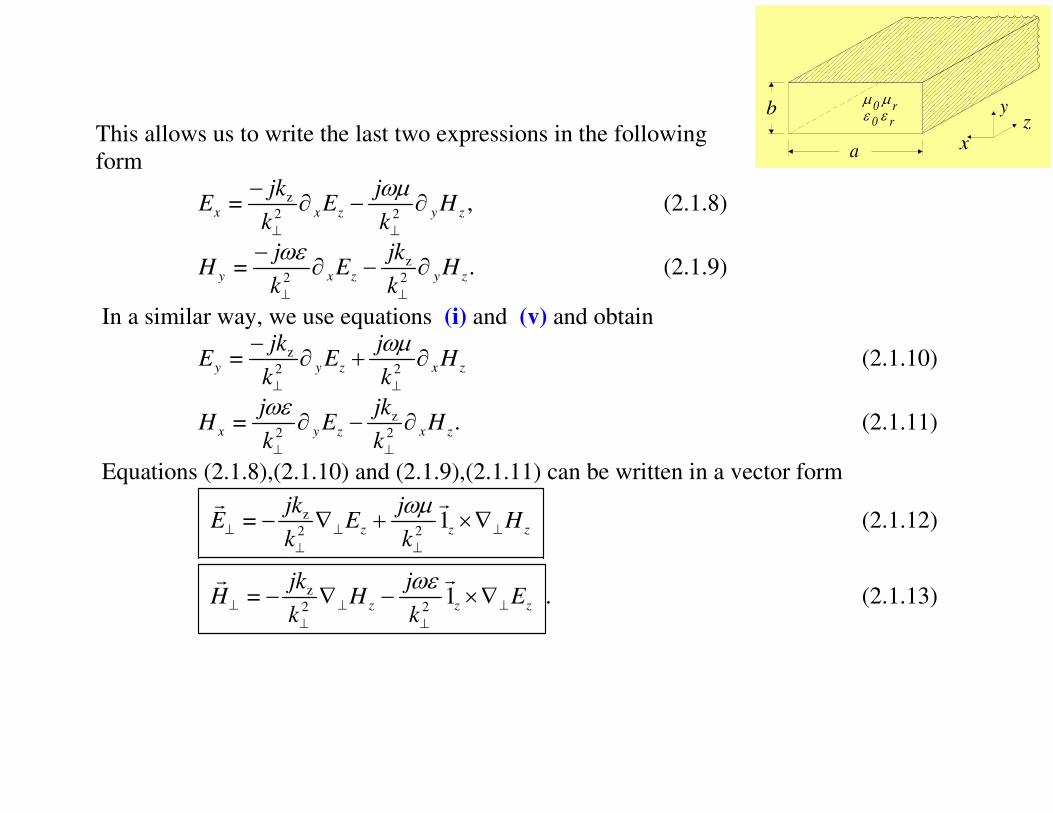
This allows us to write the last two expressions in the following
form
z
2 2= ,x x z y z
jk jE E H
k k
ωµ
⊥ ⊥
−∂ − ∂ (2.1.8)
z
2 2= .y x z y z
j jkH E H
k k
ωε
⊥ ⊥
−∂ − ∂ (2.1.9)
In a similar way, we use equations (i) and (v) and obtain
z
2 2=y y z x z
jk jE E H
k k
ωµ
⊥ ⊥
−∂ + ∂ (2.1.10)
z
2 2= .x y z x z
j jkH E H
k k
ωε
⊥ ⊥
∂ − ∂ (2.1.11)
Equations (2.1.8),(2.1.10) and (2.1.9),(2.1.11) can be written in a vector form
z
2 2= 1z z z
jk jE E H
k k
ωµ⊥ ⊥ ⊥
⊥ ⊥
− ∇ + ×∇
(2.1.12)
z
2 2= 1 .z z z
jk jH H E
k k
ωε⊥ ⊥ ⊥
⊥ ⊥
− ∇ − ×∇
(2.1.13)
µ0µ
rε 0 ε r
x
yz
a
b

Comments:
1. The wave equations for zE and zH with the corresponding boundary conditions and
the relations in ((2.1.12)--(2.1.13)) determine the electromagnetic field in the entire
space (at any time).
2. Note that the only assumption made so far was that in the z direction the
propagation is according to ( )zexp jk z− . No boundary conditions have been
imposed so far.
3. Therefore it is important to note within the framework of the present notation that
TEM mode ( = 0, = 0)z zH E is possible provided that 0k⊥ ≡ or substituting in the
wave equations
2 2= 0; = 0.E H⊥ ⊥ ⊥ ⊥∇ ∇
(2.1.14)
4. By the superposition principle and the structure of ((2.1.12)--(2.1.13)), the ransverse
field components may be derived from the longitudinal ones.
Complete Solution = ( = 0) and( = 0) ( = 0) and ( = 0)
Transverse Electric(TE) Transverse Magnetic(TM)
z z z zE H E H/ /+
.

2.2 Transverse Magnetic (TM) Mode [ = 0zH ]
In this section our attention will be focused on a specific case where = 0zH . This
step is justified by the fact that equations ((2.1.12)--(2.1.13)) are linear, therefore by
virtue of the superposition principle (e.g. circuit theory) and regarding zH and zE as
sources of the transverse field, we may turn off one and solve for the other and vice
versa. As indicated in the last comment of the previous section, the overall solution is,
obviously the superposition of the two. The boundary conditions impose that the
longitudinal electric field zE vanishes on the metallic wall therefore
z ,
,
= sin sin .z
n m
z nm
n m
jkmx nyE A e
a b
π π −
∑ (2.2.1)
This further implies that the transverse wave vector, k⊥ , is entirely determined by the
geometry of the waveguide (substitute in (2.1.3))
2 2 22 2
z2= = .
v
m nk k
a b
π π ω⊥
+ −
(2.2.2)
From these two equations we obtain
µ0µ
rε 0 ε r
x
yz
a
b

2 22 22 2
z, , 2 2
2 22
z 2
= =v v
= .v
n m
m nk k
a b
m nk
a b
ω ω π π
ω π π
⊥ − − −
± − −
(2.2.3)
This expression represents the dispersion equation of the electromagnetic wave in the
waveguide.
Exercise 2.1: Analyze the effect of the material characteristics on the cut-off frequency.
Exercise 2.2: What is the impact of the geometry?
Exercise 2.3: Can two different modes have the same cut-off frequency?!
What is the general condition for such a degeneracy to occur?
µ0µ
rε 0 ε r
x
yz
a
b

Comments:
a) Asymptotically ( vkω ⊥ ) this dispersion relation behaves as if
no walls were present i.e. zvkω .
b) There is an angular frequency c, ,n mω for which the wavenumber zk vanishes. This is
called the cutoff frequency.
( ) ( )2 2 2 2
, ,
1v = v = v ,
2c m n mc n
m nf
m nk
a b a b
π πω ⊥
≡ + ⇒ +
(2.2.4)
where v = /r r
c ε µ .
c) Below this frequency the wavenumber zk is imaginary and the wave decays or grows
exponentially in space.
d) The indices n and m define the mode ,m nTM ; m
represents the wide transverse dimension ( x ) whereas n
represents the narrow transverse dimension ( y ).
µ0µ
rε 0 ε r
x
yz
a
b
12cω
11cω
zk
ω
vkz=ω

2.3 Transverse Electric (TE) Mode [ = 0zE ]
The second possible solution according to (2.1.12)--(2.1.13) is when = 0zE and
since the derivative of the longitudinal magnetic field zH vanishes on the walls (see
(2.1.12)) we conclude that
z ,,
,
= cos cos .z
m n
z m n
m n
jkmx nyH A e
a b
π π −
∑ (2.3.1)
The expression for the transverse wavenumber k⊥ is identical to the TM case and so is
the dispersion relation. However, note that contrary to the TM mode where if n or m
were zero the field component vanishes, in this case we may allow = 0n or = 0m
without forcing a trivial solution.
µ0µ
rε 0 ε r
x
yz
a
b

For convenience, we present next a comparison table of the
various field components of the two modes. TM mode TE mode
z= sin sinzmn
z mnmn
mx ny jkE A e
a b
π π −
∑ = cos coszmn
z mnmn
mx ny jkH B e
a b
π π −
∑
2
,
= sin cosx mnmnn m
j n mx nyH A
k b a b
ωε π π π
⊥
∑ … 2
= cos sinx mnmn
j n mx nyE B
k b a b
ωµ π π π
⊥
∑ …
2
= cos siny nmn
j m mx nyH A
k a a b
ωε π π π
⊥
−
∑ … 2
= sin cosy mnmn
j m mx myE B
k a a b
ωµ π π π
⊥
−
∑ …
= 0zH = 0zE
z
2= cos sinx mnmn
jk m mx nyE A
k a a b
π π π
⊥
−
∑ … z
2= sin cosx mnmn
jk m mx myH B
k a a b
π π π
⊥
+
∑ …
z
2= sin cosy mnmn
jk n mx nyE A
k b a b
π π π
⊥
−
∑ … z
2= cos siny mnmn
jk n mx myH B
k b a b
π π π
⊥
+
∑ …
1/22
, ,( ) ( )
, ,= ; 1c m nTM TM
x mn mn y mn mn
fE Z H Z
f
µε
= −
1/ 22
, , ,( )
, ( )= ; 1
y mn c m nTE
x mn mnTE
mn
E fH Z
Z f
µε
−
− = −
( )
, ,= TM
y mn mn x mnE Z H− ,
, ( )=
x mn
y mn TE
mn
EH
Z
Exercise 2.4: Check all the expressions presented in the table above.
µ0µ
rε 0 ε r
x
yz
a
b

Comments:
1. The phase velocity of the wave is the velocity an imaginary observer has to move
in order to measure a constant phase i.e. z =t k zω − const.. This implies,
1/22
p 2
z
v = v 1 .ch
f
k f
ω−
≡ −
(2.3.2)
2. The phase velocity is always faster than v !! Specifically, in vacuum the phase
velocity of a wave is larger than c . In fact close to cutoff this velocity becomes
``infinite"!!
3. The group velocity is defined from the requirement that an observer sees a constant
envelope in the case of a relatively narrow wave packet. At the continuous limit this
is determined by
1/22
gr 2
z
v = = v 1 .cf
k f
ω ∂− ∂
(2.3.3)
4. The group velocity is alway smaller than v . Specifically, in vacuum it is always
smaller than c . It is the group velocity is responsible to information transfer.
5. When the waveguide is uniform
2
ph gv v = v .r
(2.3.4)
µ0µ
rε 0 ε r
x
yz
a
b
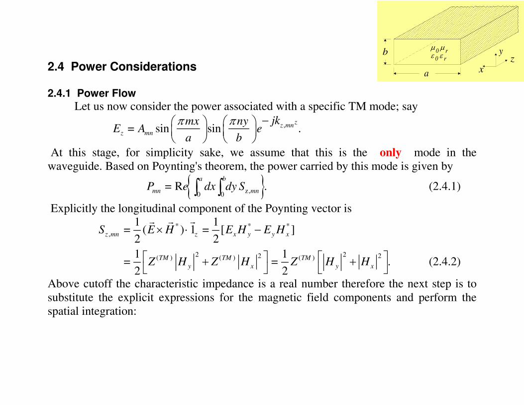
2.4 Power Considerations
2.4.1 Power Flow
Let us now consider the power associated with a specific TM mode; say
,= sin sin .z
z mn
z mn
jkmx nyE A e
a b
π π −
At this stage, for simplicity sake, we assume that this is the only mode in the
waveguide. Based on Poynting's theorem, the power carried by this mode is given by
z,0 0
= R .a b
mn mnP e dx dy S∫ ∫ (2.4.1)
Explicitly the longitudinal component of the Poynting vector is
* * *
,
2 22 2( ) ( ) ( )
1 1= ( ) 1 = [ ]
2 2
1 1= = .
2 2
× ⋅ −
+ +
z mn z x y y x
TM TM TM
y x y x
S E H E H E H
Z H Z H Z H H (2.4.2)
Above cutoff the characteristic impedance is a real number therefore the next step is to
substitute the explicit expressions for the magnetic field components and perform the
spatial integration:
µ0µ
rε 0 ε r
x
yz
a
b

2 2( )
0 0
2 22 22( )
4
2
2 22( )
2
1=
2
1=
2
1= .
2
2
4
2
a bTM
mn y x
TM
mn
k
TM
mn mn
P Z dx dy H H
m nZ A
k a b
abP Z A
k
a bω ε π π
ω ε
⊥
⊥
⊥
+
+
⋅
∫ ∫
(2.4.3)
The last expression represents the average power carried by the specific mode.
Exercise 2.5: What is the power at any particular point in time?
Exercise 2.6: Since the two sets sin( / )mx aπ and sin( / )ny bπ are two orthogonal sets of
functions, the total average power carried by the wave in the forward direction is a
superposition of the average power carried by each individual mode separately. In other
words show that ,
=mnn m
P P∑ .
Exercise 2.7: Show that below cutoff, the power is identically zero although the field is
not zero.
µ0µ
rε 0 ε r
x
yz
a
b

Exercise 2.8: Note that the average power is proportional to the
average magnetic energy per unit length. Calculate this quantity. Compare it with the
average electric energy per unit length.
Exercise 2.9: Calculate the energy velocity of a specific mode v = /EM EMP W⟨ ⟩ . Compare
to the group velocity. What happens if the frequency is below cutoff?
Exercise 2.10: Repeat the last exercise for a superposition of modes ,n mA .
µ0µ
rε 0 ε r
x
yz
a
b

2.4.2 Ohm Loss
So far it was assumed that the walls are made of an ideal metal ( )σ →∞ . If this is
not the case (σ ) a finite amount of power is absorbed by the wall. In order to calculate
this absorbed power we firstly realize that the magnetic field is ``discontinuous" which is
compensated by a surface current
= .sJ n H×
(2.4.4)
This current flows in a very thin layer which is assumed to be on the scale of the skin-
depth [ = /sJ J δ ] therefore, the dissipated average power per unit length is given by
21 1
= ,2
D sP dxdy Jδσ ∫
(2.4.5)
or explicitly
22 21 1
= = = ,2 2 2
s sD s s
J RP dl dl J dl Jδ
σ δ δσ∫ ∫ ∫
(2.4.6)
where 2 / oδ ωµ σ≡ , / 2s oR ωµ σ≡ and the integration is over the circumference of
the waveguide
µ0µ
rε 0 ε r
x
yz
a
b

21
= .2
D s sP R dl J∫
(2.4.7)
This is the average electromagnetic power per unit length which is converted into heat
(dissipation) due to Ohm loss. Based on Poynting's theorem we may deduce that the
spatial change in the electromagnetic power is given by
D
dP P
dz= − (2.4.8)
and since in case of a single mode both P and DP are proportional to 2| |A ,
2 2
and∝ ∝DP A P A (2.4.9)
we conclude that the change in the amplitude of the mode is given by
2
2 2 2 2= 2 ( ) = ( = 0) .d A z
A A z A z edz
αα −− ⇒ (2.4.10)
The coefficient α represents the exponential decay of the amplitude and based on the
arguments of above is given by
.2
DP
Pα ≡ (2.4.11)
Let us denote by (0)
zk the wavenumber in a lossless waveguide. Subject to the
µ0µ
rε 0 ε r
x
yz
a
b
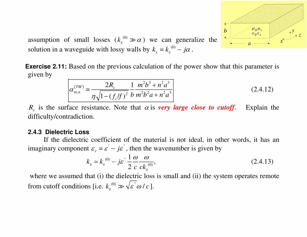
assumption of small losses ((0)
zk α ) we can generalize the
solution in a waveguide with lossy walls by (0)
z z=k k jα− .
Exercise 2.11: Based on the previous calculation of the power show that this parameter is
given by
( )
2 3 2 3
, 2 2 2 32
2 1=
1 ( / )
TM sm n
c
R m b n a
b m b a n af fα
η
++−
(2.4.12)
sR is the surface resistance. Note that α is very large close to cutoff. Explain the
difficulty/contradiction.
2.4.3 Dielectric Loss
If the dielectric coefficient of the material is not ideal, in other words, it has an
imaginary component =' ''
r jε ε ε− , then the wavenumber is given by
(0)
z z (0)
z
1,
2
''k k j
c ck
ω ωε− (2.4.13)
where we assumed that (i) the dielectric loss is small and (ii) the system operates remote
from cutoff conditions [i.e. (0)
z /''k cε ω ].
µ0µ
rε 0 ε r
x
yz
a
b

We can now repeat the entire procedure described in the
previous subsection for a TE mode. Here are the main steps and
results
( )
,
,0 0
22* *
, ( )
= cos cos , = e ,
1 1= = .
2 2
a bzz mn
z mn mn z mn
z mn x y y x x yTEmnmnmn
jkmx nyH A e P R dx dyS
a b
S E H E H E EZ
π π −
− +
∫ ∫
(2.4.14)
2 22 2 2 2
2
( ) 4 4
2 22
( ) 2
1 1 1 1 1 1=
2 2 2 2 2
1=
8
mn mnTE
mn
mnTE
mn
n mP A a b a b
Z k b k a
abA
Z k
ω µ π ω µ π
ω µ
⊥ ⊥
⊥
+ (2.4.15)
2 3 2
( )
1/2 2 2 22
2 1 ( / )= .
( / )1 ( / )
TE smn
c
R m b a n
b m b a nf fα
η
++ −
(2.4.16)
µ0µ
rε 0 ε r
x
yz
a
b

Exercise 2.12: Check equation (2.4.16). In particular check the cases = 0n or = 0m .
Repeat all the exercises from the above (TM mode) for the TE mode. Make a comparison
table where relevant.
Exercise 2.13: Note that both ( )TEα and ( )TMα are large close to cutoff and increase as
ω for large frequencies. In between there is a minimum loss for an optimal
frequency. Calculate it.
Exercise 2.14: Calculate the loss very close to cutoff.

2.5 Mode Comparison
Mode comparison for a rectangular waveguide.

2
3
x
y z
2
3
1
x
y z
1
2
3
x
y z
1
z
23
1
x
yz
2
3
1
2
3
1
x
yz
1
23
10TE
1
23
21TE
1
23
11TE
1
23
20TE
1
23
11TM
1
23
21TM

2.6 Cylindrical Waveguide
2.6.1 Transverse Magnetic (TM) Mode [ = 0]zH
In this section we shall investigate the propagation of a wave in a cylindrical
waveguide. The longitudinal component of the electric field satisfies
2 2
[ ] = 0,zk E⊥ ⊥∇ + (2.6.1)
where 2
2 2
2=
vz
k kω
⊥ − or explicitly
2 2
2
2 2 2
1 1= 0.zk E
r r r r ϕ ⊥
∂ ∂ ∂+ + + ∂ ∂ ∂
(2.6.2)
The solution of this equation subject to the boundary conditions ( = ) = 0zE r R reads
[ ]z ,
,
,
= cos( ) sin( ) ,z
s n
z n s n ns ns
n s
jkrE J p e A n B n
Rϕ ϕ
− +
∑ (2.6.3)
where ( )nJ u if the n 'th order Bessel function of the first kind. This function behaves
similar to a trigonometric function (sin or cos ). It has zeros, denoted by ,s np i.e.,
, ,: ( ) 0.s n n s n
p J p ≡

The first few zeros of the Bessel function are tabulated next.
s=1 s=2 s=3
n= 0 2.405 5.52 8.654
n=1 3.832 7.016 10.174
n=2 5.135 8.417 11.62
Substituting (2.6.3) in (2.6.2) we obtain
22 2,
2 2 2
1 1= 0
s n
z
pE
r r r r Rϕ
∂ ∂ ∂+ + + ∂ ∂ ∂
(2.6.4)
thus
22,2 2
2
22,2
z , 2 2== .
v v
s s
n
n
sz
np
kR
pk k
R
ωω⊥
≡ − ⇒ −
(2.6.5)
Based on this expression the characteristic impedance of the TM mode is given by
z, ,( )
,
v= .
s nTM
s n
kZ η
ω (2.6.6)

2.6.2 Transverse Electric (TE) Mode [ = 0]zE
In this case the wave equation reads
2 2
[ ] = 0zk H⊥ ⊥∇ + (2.6.7)
and its solution has the form
z ,
, , ,
,
= cos( ) sin( ) ,z
s n
z n s n s n s n
s n
jkrH J p e A n B n
Rϕ ϕ
− ′ + ∑ (2.6.8)
where
, ,
=
= 0 : ( ) = 0.zs n n s n
r R
Hp J p
r
∂ ′ ′ ′⇒∂
(2.6.9)
The first few zeros of the derivatives of the Bessel function are
s=1 s=2 s=3
N=0 3.832 7.016 10.174
N=1 1.841 5.331 8.536
N=2 3.054 6.706 9.970
thus
22
,( )
, z, ,
, ,
= , =v v
s nTE
s n s n
z s n
pZ k
k R
ω ωη
′ −
(2.6.10)

Summary
( )
2
,
2
,
TE modes TM modes
cos0
sin
cos0
sin
cos/
sin
sin
cos
zsn
z n sn
zsn
z n sn
z TMsn sn snr n sn sn
sn
zsn snn sn
sn
nr jkH J p e
nR
nr jkE J p e
nR
njk p r jkH J p e E Z
nRk R
njnk r jkH J p e
rk R
ϕ
ϕ
ϕϕ
ϕϕ
ϕϕ
ϕ
′⊥
⊥
− ′=
− =
′ − ′= − −
−− ′= −
( )
( )
2
,
( )
2
,
1/2 1/22 22 2
2 2
(
/
cos
sin
sin
cos
v v
TM
r sn
zTE sn sn snr sn n sn
sn
zTE sn snsn r n sn
sn
sn snsn
T
sn
E Zn
njk p r jkE Z H J p e
nRk R
njnk r jkE Z H J p e
nrk R
p pk
R R
Z
ϕ
ϕ
ϕ
ϕϕ
ϕϕ
ω ω
′⊥
⊥
− = −
−− = − −
′ = − −
) ( )
,
v
v
/ /
E TM snsn
sn
sn sn sn
kZ
k
k p R p R
ωη η
ω
⊥
= =
′=

'2 2 2 2 20 0,4 4
, 0, , 0,
1/2 1/22 2 2 2 2 22
, , ,
2 2 '2 2 2
TE modes TM modes
Power= ( ) ( ) [ ( )]2 2
v v1 1
sn snsn n sn sn n sn
sn n sn n
sn sn sns s
sn
k k k kp n J p p J k R
k g k g
k k c kR n R
R p n R
η π η π
αη ω ω η ω
⊥⊥ ⊥
− −
⊥ ⊥ ⊥
′ ′−
= − + −
−
00,
00 0
1 = 01
v= , = =
2 = 0
rn
rr r
n
g
n
µ µη
ε εµ µ ε ε
/

2.6.3 Power Considerations
According to Maxwell's Equations for a single mode we have
2
= , = , = / .z rz r TM
TM
jk EE E H H E Z
k Zϕ ϕ⊥ ⊥
⊥
− ∇ −
Consequently, the average Poynting vector is
( )*1= 1
2z zS E H⊥ ⊥× ⋅
and the average power flowing in the waveguide
* * *
. . . .
22
22
. . . .
22
2 2
2 4. . . .
1 1= Re = Re
2 2
1 | | 1= e = Re
2 2
1 1= Re = Re
2 2
r rc s c sz
rr
c s c sTM TM TM
z zz z
c s c sTM TM
P da E H da E H E H
EER da da E E
Z Z Z
k kda E da E
Z k Z k
ϕ ϕ
ϕϕ
⊥ ⊥
⊥ ⊥⊥ ⊥
× −
+ +
∇ ∇
∫ ∫
∫ ∫
∫ ∫
. (2.6.11)
In order to further simplify the last expression let us examine the wave equation:
( )2 2 = 0zk E⊥ ⊥∇ + (2.6.12)

we multiply by the complex conjugate of zE
( )* 2 2 = 0z zE k E⊥ ⊥∇ + (2.6.13)
and integrate over the entire cross section
( )
2* 2 2
2 2* 2
= 0
= 0.
⊥ ⊥
⊥ ⊥ ⊥ ⊥
∆ ∇ +
∆ ∇ ∇ − ∇ +
∫
∫
z z z z
z z z z z
da E E k E
da E E E k E (2.6.14)
The first term in the integrand is zero since
* *= = 0z z z zda E E d E E⊥ ⊥ ⊥ ⊥ ∇ ∇ ⋅ ∇ ∫ ∫
hence
2 22= .z zda E k da E⊥ ⊥∇∫ ∫ (2.6.15)
Now back to the propagating power for a superposition of modes starting from the
expression for a single mode we get
( ) ( )
2 22 2
, 4 2
,
, ,2 ,
0 0
', ' ' ', '
', '
1 1= Re =
2 2
cos( )1
=2 / v
cos( ' )
zs n z zTM TM
s n
zs n n s n
R s n
s n n s n
s n
k kP da E da E
k kZ Z
k rA J p n
k RP d drr
rA J p n
k R
π
ϕ
φη ω
ϕ
⊥⊥ ⊥
⊥
⊥
∇
∫ ∫
∑∫ ∫
∑
The integration over the angle it is sraight forward
2
, '0
1 = 0
cos( )cos( ' ) 2 , = 1= 0
2
n n n n
n
d n n g gn
πφ ϕ ϕ π δ
= /
∫
and after integration over r we get
( )
2 22, , 2
, ,2, , , ,,
1=2 ( )
22
z s n
n s n n s n ssTMn s s s ns n
k RP g A J p
kZπ δ ′
′ ⊥
′ ∑
where we used
2
2
, , ' , , '0
( )2
R
n n s n n s n n s s s
r r Rdr r J p J p J p
R Rδ ′ = ∫ (2.6.16)

In the case of a single mode we have
222
2, ,
, , 2 2
,
( )1= Re .
2 v v
s n n s n
s n s n n
s n
p J pP RA R R g
R p
ω ωπ
η
′ − (2.6.17)
Note that there is power flow only if the wave is above cutoff and as in the rectangular
case, the the total power is the superposition of the power in each mode separately
Exercise 2.15: Calculate the average energy per unit length stored in the
electromagnetic field.

2.6.4 Ohm Loss
Now to the general expression for the losses. Starting from the dissipated power
( )
( )
( )
( )
22 2 ,( )
,1bound
2
22 2
2
222
2
1 1= = =
2 2 2
1= 2
2
1= 2
2 v
r snsusuD sn z s s TM
sn
n nssn sn
TMns
sn
n nssn sn
ns
ERP J d R H d R d
Z
J pRk R g A R
pRZ
J pRR g A R
pR
φ
π
ωπ
η
′
′
∫ ∫ ∫
(2.6.18)
which finally entails for a single mode
,( ) 1
= .ph snTM s
ns
vR
R vα
η
(2.6.19)
Exercise 2.16: Check Eq. (2.6.19).
Exercise 2.17: Calculate ( )TE
nsα .
Exercise 2.18: Calculate the exponential decay due to dielectric loss.

Mode comparison for cylindrical waveguide.
0 0.4 0.8 1.2 1.6 20 24 28 32 36 400
0.002
0.004
0.006
0.008
0.010
Att
enua
tion
, dec
ibel
s/m
eter
DiameterWavelength
Attenuation due to copper losses in circular waveguides at 3000 Mc/sec.1 2 30
Relative cutoff frequencies of waves in a circular guide.
1000 5000 9000 13000
0.01
0.02
0.03
0.04
0.05
0.06
0.07
Att
enua
tion
, dec
ibel
s/m
eter
Frequency, megacycles/second
Attenuation due to copper losses in circularwaveguides; diameter = 2 in.
11TE 21TE 01TE 31TE 41TE 12TE
01TM 11TM21TM 02TM
( )11TEfc
11TE
01TM
01TE
11TE 01TM 01TE
fel

Wave Type TM 01 TM 02 TM11 TE 01 TE11
Field distribution
in cross-sectional
plane, at plane of
maximum
transverse fields
Field distribution
along guide
DistributionsBelow Along
This Plane
DistributionsBelow Along
This Plane
Field components
present , ,z rE E Hϕ , ,z rE E Hϕ , , , ,z r rE E E H Hϕ ϕ , ,z rH H Eϕ , , , ,z r rH H H E Eϕ ϕ
p or p′ 2.405 5.52 3.83 3.83 1.84
( )ck 2.405
α
5.52
α
3.83
α
3.83
α
1.84
α
( )cλ 2.61α 1.14α 1.64α 1.64α 3.41α
( )cf
0.383
α µε
0.877
α µε
0.609
α µε
0.609
α µε
0.293
α µε
Attenuation due to
imperfect
conductors 2
1
1 ( / )
s
n c
R
f fα −
2
1
1 ( / )
s
n c
R
f fα −
2
1
1 ( / )
s
n c
R
f fα −
2
2
( / )
1 ( / )
s c
n c
R f f
f fα −
2
1
1 ( / )
s
n c
R
f fα −

2.7 Pulse Propagation
Let us consider an azimuthally symmetric TM mode described by
[ ]0
=1
( , , ) = ( ) exp ( )z s s s
s
rE r z t J p d j t z
Rω ω ω
∞ ∞
−∞−Γ∑ ∫ E (2.7.1)
wherein 2 2 2 2 2
= / /s sp R cωΓ − and ( )s ωE is the Fourier transform of this field component
at = 0z
( )02 02
1
1 1( ) = exp ( , = 0, ).
2( )
2
R
s s z
s
rdr r J p dt j t E r z t
R RJ p
ω ωπ
∞
−∞
′ ′ ′ ′ ′ ′− ∫ ∫E (2.7.2)
Let us now calculate the energy associated with the radiation field as it propagates in
an empty waveguide. The transverse field components are
( )
( )
1 22=1
2
1 222=1 0
2
( , , ) = exp
1( , , ) = exp
s s sr s s
s
s
s ss s
s
s
prE r z t J p d j t z
R R
c
pr jH r z t J p d j t z
R R c
c
ϕ
ω ωω
ωω ω
ωµ
∞
−∞
∞ ∞
−∞
Γ −Γ Γ +
−Γ Γ +
∑ ∫
∑ ∫
E
E (2.7.3)
therefore, the z -component of the Poynting vector is

( )
( )
1
=1
1
=1 0
( , , ) = exp ( )
1exp ( ) ( ) .
z s s s s
s s
r RS r z t J p d j t z
R p
r RJ p d j t z j
R cpσ σ σ
σ σ
ω ω ω
η
∞ ∞
−∞
∞ ∞
−∞
− Γ Γ
× Ω Ω −Γ Ω Ω Ω
∑ ∫
∑ ∫
E
E (2.7.4)
Using the orthogonality of Bessel functions
2
2
1 1 10
= ( )2
R
s s s
r r RdrrJ p J p J p
R Rσ σδ
∫ (2.7.5)
the power propagating is
( )
( )
22
1
=1
0
( , ) = 2 ( ) exp ( )2
1exp ( )
s s s s
s s
s s
s
R RP z t J p d j t z
p
Rd j t z j
cp
π ω ω ω
η
∞ ∞
−∞
∞
−∞
−Γ Γ
× Ω Ω −Γ Ω Ω
∑ ∫
∫
E
E (2.7.6)
and the energy associated with this power

( ) ( )
( ) [ ]
22
1
=1
0
( ) = ( , )
= (2 ) ( ) ( )exp ( )exp2
1 1exp ( ) .
R
s s s s s
s
s
s s
W z dtP z t
RJ p d z d z
Rj R dt j t
p c p
π ω ω ω
ω ωη
∞
−∞
∞
∞
−∞
−Γ Ω Ω −Γ Ω
Ω× Γ +Ω
∫
∑ ∫ ∫
∫
E E
(2.7.7)
With the definition of the Dirac delta function 1 ( )
( )2
j tdt e
ωδ ωπ
+ΩΩ+ ≡ ∫ we have
( ) ( ) 2
2 2
1
=1
( ) = (2 ) ( ) ( ) ( )exp2
( ) 1 1.
R s s s s s
s
s
s o s
RW z J p d z
Rj R
p c p
π ω ω ω ω ω
ω ωη
∞ ∞
−∞ − − Γ + Γ −
Γ× −
∑ ∫ E E
(2.7.8)
For proceeding it is important to emphasize two features: since the field components are
real functions, it is evident that the integrand ought to satisfy *
( ) = ( )s sω ω−F F .
Consequently
*
( ) = ( )s sω ω−E E (2.7.9)
and
*
( ) = ( ).s sω ωΓ − Γ (2.7.10)

This last conclusion implies that if the frequency is below cut-off (| |< / )sp c Rω then
( ) =| ( ) |s sω ωΓ − Γ (2.7.11)
whereas if | |> /scp Rω
( ) = | ( ) |.s sjω ωΓ − − Γ (2.7.12)
With these observations we conclude that
( )2 2/
2 2
10
=10
2
/
2(2 )( ) = ( )2Re | ( ) |
2
| ( ) | | ( ) || ( ) | .
cp R ss
R s s
s
s ss
cp Rss s s s
zRW z J p d e
R Rj R Rd
cp p cp p
ωπω ω
η
ω ωω ωω ω
∞
∞
− Γ
Γ Γ− × +
∑ ∫
∫
E
E
(2.7.13)
Clearly the first integrand is pure imaginary therefore, its contribution is identically
zero and as a result, in the lossless case considered here, the energy associated with the
propagating signal does not change as a function of the location 2 2
2 2
1/
=10
| ( ) |(2 )= ( ) 2 | ( ) | .
2
ss s
cp Rss s s
RR RW J p d
cp p
ωπ ωω ω
η
∞ ∞ Γ
∑ ∫ E (2.7.14)

Comments:
1. Only the propagating components contribute to the radiated energy.
2. The non-propagating components are confined to the close vicinity of the input
(where initial conditions were defined).
3. If all the spectrum is confined to the region 10 < < /p c Rω , no energy will
propagate.
4. Since the waveguide is lossless, the propagating energy does not change as a
function of z .
Exercise 2.19: Calculate the electromagnetic energy per unit length. Compare with
(2.7.14).
Let us now simplify the discussion and focus on a source which excites only the first
mode ( = 1)s i.e., 0 1 0( , = 0, ) = ( / ) ( )zE r z t J p r R E t therefore according to Eq.(2.7.2) we get
0 0 1 02 02
1
,1
0
1 1( ) = ( ')
2( )
2
= ( ')2
R
s s
s
s
r r j tdr r J p J p dt e E t
R R RJ p
j tdt e E t
ωωπ
δ ωπ
∞
−∞
∞
−∞
′ −′ ′ ′
′−′
∫ ∫
∫
E
(2.7.15)

As an example, consider a signal starting from t=0 ramping up and oscillating
and decaying
( ) ( )( )
2,1
0 0 0 2 2 2( ') sin exp ( ) =
2 1 2
s
s
t TE t E t h t E
T j T T
δω
π ω ωΩ = Ω − ⇒
+ + Ω − E (2.7.16)
Substituting in Eq.(2.7.14)
( )( )( ) ( )1
2 4 2 221
2 4 1 10 22 2/ 2 2 210 1
1 ( )=
1 2cp R
TJ pW E R d
c p T Tω
ω ω ωω
η ω ω
∞
=
Ω −
+ Ω − + ∫ (2.7.17)
Normalizing to the cutoff frequency, 1/u ω ω= as well as 1 1/ , T Tω ωΩ =Ω = the last
integral simplifies to read
2 2
2 3 21 10 0 21 2 2 2 2 2
1
( ) 1=
4
J p u uW E R du
p T u u Tε
∞
− −
−Ω
+Ω − + ∫ (2.7.18)
Its numerical analysis reveals that
2
2 3 21 10 0
1
1 1( )
4 1
J pW E R
p T
πε
Ω <Ω
Ω >∼ (2.7.19)
Exercise 2.20: Compare with the dependence of the propagating energy in the frequency
Ω when the signal prescribed by Eq.(2.7.16) propagates in free space.

2.8 Waveguide Modes in Coaxial Line

Chapter 3: Waveguides – Advanced Topics
After paving the foundations of electromagnetic phenomena in waveguides, in this chapter we shall consider some advanced phenomena including:
1. Hybrid modes, whereby the TM and TE are coupled 2. Dielectric loaded waveguide 3. Mode coupling due to geometric discontinuity 4. Reactive elements 5. Excitation of Waveguides 6. Coupling between two waveguides 7. Surface waveguides 8. Transients 9. Cavities 10. Wedge in a Waveguide

3.1 Hybrid Modes In Section 2.1 it was demonstrated that if the waveguide's electromagnetic
characteristics are uniform on the cross-section, the transverse components may be derived from the two longitudinal components that in turn are independent. For example in a rectangular waveguide we had
,
,,
,
,,
( , , ; ) = sin sin
( , , ; ) = cos cos
zn nx yz n n x yx y
n n x yx y
zm mx yz m m x yx y
m m x yx y
x yE x y z A n n ea a
x yH x y z B m m ea a
γω π π
γω π π
−⎛ ⎞⎛ ⎞⎜ ⎟⎜ ⎟ ⎜ ⎟⎝ ⎠ ⎝ ⎠
−⎛ ⎞⎛ ⎞⎜ ⎟⎜ ⎟ ⎜ ⎟⎝ ⎠ ⎝ ⎠
∑
∑ (3.1.1)
wherein ( )22 2r r= /k cγ ε μ ω⊥ − and ( ) ( )222 = / /x x y yk n a n aπ π⊥ + for the transverse
magnetic (TM) mode or ( ) ( )222 = / /x x y yk m a m aπ π⊥ + for the transverse electric (TE) mode. The transverse components being given by
2 2 2 2= 1 , = 1z zz z z zE E H H Ej jk k k k
Hγ ωμ γ ωε⊥ ⊥ ⊥ ⊥
⊥ ⊥ ⊥ ⊥⊥ ⊥− ∇ + ×∇ − ∇ − ×∇ (3.1.2)

Let us now assume that the relative dielectric coefficient r( )ε depends on the transverse coordinates (e.g. x and y in a rectangular geometry) and so is the relative permeability coefficient r( )μ , the goal being to determine the character of the modes supported by the structure. Our starting point again is Maxwell's equations
0 r 0 r
r 0 r
= ( ) = 0
= ( ) = 0o
E j H H
H j E E
ωμ μ μ μ
ωε ε ε ε
∇× − ∇ ⋅
∇× ∇ ⋅ (3.1.3)
which lead to the following wave equations
0 r 0 r r
20 r r 0 r
22
r r 0 r2
( ) = ( ) = [ ]
( ) = [ ( )]
= ( ) 1
∇× ∇× − ∇× − ∇ × + ∇×
−∇ +∇ ∇⋅ − ∇ × +
⎡ ⎤ ⎡ ⎤∇ + ∇ ∇⋅ + ∇ ×⎢ ⎥ ⎣ ⎦⎣ ⎦z z
E j H j H H
E E j H j E
E E j Hc
ωμ μ ωμ μ μ
ωμ μ μ ωε ε
ω ε μ ωμ μ (3.1.4)
Bearing in mind Gauss' law r r( ) = 0 = lnE E Eε ε∇ ⋅ ⇒∇ ⋅ − ⋅∇ we get 2
2 2r r r 0 r r2 = ( ln ) ( ln ) 1z zE E j H
cωγ ε μ γ ε ωμ μ μ⊥ ⊥ ⊥ ⊥ ⊥
⎡ ⎤∇ + + ⋅∇ + ∇ × ⋅⎢ ⎥⎣ ⎦
(3.1.5)

and in a similar way 2
2 2r r r 0 r r2 = ( ln ) ( ln ) 1z zH H j E
cωγ ε μ γ μ ωε ε ε⊥ ⊥ ⊥ ⊥ ⊥
⎡ ⎤∇ + + − ⋅∇ − ∇ × ⋅⎢ ⎥⎣ ⎦
(3.1.6)
It is evident from these two equations (3.1.5)--(3.1.6) that zE and zH are no longer independent if transverse variations in the cross-section occur. Modes which are linear combinations of TE and TM modes are called hybrid modes and they frequently occur in microwave components.
In order to illustrate the coupling of TE and TM modes let us consider a dielectric loaded waveguide as illustrated in the figure. A fraction of the waveguide (0 < )x d≤ is filled with dielectric material r( )ε whereas the remainder ( < )d x a≤ has the same characteristics as the vacuum. In each region the material is uniform which means that the wave equation is
x
y
a
b
d
εr

2
r2 22 = 0
1 zEc
ε ω γ⊥
⎡ ⎤⎛ ⎞∇ + +⎢ ⎥⎜ ⎟
⎝ ⎠⎣ ⎦ (3.1.7)
and its solution is 2 2
2r 2
2 22
2
sinh 0
= sin
sinh ( )
z
mA x x db cyzE e m
b mB x a d x ab c
π ωγ εγ π
π ωγ
⎧ ⎡ ⎤⎛ ⎞⎪ ⎢ ⎥− − ≤ ≤⎜ ⎟⎪ ⎢ ⎥⎝ ⎠⎪ ⎣ ⎦⎛ ⎞−⎨⎜ ⎟
⎝ ⎠ ⎡ ⎤⎪ ⎛ ⎞⎢ ⎥− − − ≤ ≤⎪ ⎜ ⎟⎢ ⎥⎝ ⎠⎪ ⎣ ⎦⎩
(3.1.8)
wherein we impose the boundary condition at = 0x and =x a . Similarly, for zH we have
2
r2 22 = 0
1 zHc
ε ω γ⊥
⎡ ⎤⎛ ⎞∇ + +⎢ ⎥⎜ ⎟
⎝ ⎠⎣ ⎦ (3.1.9)
and
x
y
a
b
d
εr

2 22
r 2
2 22
2
cosh 0
= cos
cosh ( )
z
mC x x db cmzH e y
b mD x a d x ab c
π ωγ επγ
π ωγ
⎧ ⎡ ⎤⎛ ⎞⎪ ⎢ ⎥− − ≤ ≤⎜ ⎟⎪ ⎢ ⎥⎝ ⎠⎪ ⎣ ⎦⎛ ⎞−⎨⎜ ⎟
⎝ ⎠ ⎡ ⎤⎪ ⎛ ⎞⎢ ⎥− − − ≤ ≤⎪ ⎜ ⎟⎢ ⎥⎝ ⎠⎪ ⎣ ⎦⎩
(3.1.10)
Imposing the boundary condition at x=d leads us to the dispersion relation. In order to emphasize the coupling between TE and TM modes we shall develop the dispersion relation in two stages. Stage I: we impose the continuity of zE and zH facilitating to redefine the amplitudes thus A and D according to
[ ][ ]
v
v
sinh( ) 0sinh( )
= sinsinh ( )sinh ( )
z
x x ddyzE Ae m
a xbd x a
a d
ε
εγ π
Λ⎧ ≤ ≤⎪ Λ⎪⎛ ⎞−⎨⎜ ⎟ Λ −⎝ ⎠⎪ ≤ ≤⎪ Λ −⎩
(3.1.11)
and
x
y
a
b
d
εr

[ ][ ]
v
v
cosh( ) 0cosh( )
= coscosh ( )cosh ( )
z
x x ddyzH De m
a xbd x a
a d
ε
εγ π
Λ⎧ ≤ ≤⎪ Λ⎪⎛ ⎞−⎨⎜ ⎟ Λ −⎝ ⎠⎪ ≤ ≤⎪ Λ −⎩
(3.1.12)
wherein ( ) ( )2 22 2/ /m b cε π γ ε ωΛ ≡ − − is the horizonthal wave number in the dielectric
(subscript ε ) and ( ) ( )2 22 2v / /m b cπ γ ωΛ ≡ − − represents the horizonthal wave number in
the vacuum (subscript v). It is evident that if = 0d or =d a (i.e. the waveguide is filled uniformly), the regular solutions may be readily retrieved v =a j nπΛ or =a j nε πΛ . Stage II: In our second step if 0 < <d a we need to impose continuity of yE and yH at
=x d . According to (3.1.2) the transverse components are
02 2
2 2r r2 2
0 r2 2
2 2r r2 2
=
=
− ∂ + ∂+ +
− ∂ − ∂+ +
y y z x z
y y z x z
jE E H
c cj
H H E
c c
ωμγω ωγ ε γ ε
ωε εγω ωγ ε γ ε
(3.1.13)
x
y
a
b
d
εr

Based on (3.1.13) and (3.1.11)-(3.1.12) we get
02 2
2 2r r2 2
02 2
2 22 2
( = 0) = tanh( )
( = 0) = tanh[ ( )]
⎛ ⎞− + Λ Λ⎜ ⎟⎝ ⎠+ +
+ − Λ Λ −+ +
y
y v v
jmE x d A D db
c cjmE x d A D a d
bc c
ε εωμγ π
ω ωγ ε γ ε
ωμγ πω ωγ γ
(3.1.14)
thus their continuity implies
[ ]02 2 2 2
2 2 2 2r r2 2 2 2
tanh ( ) tanh( )= v v
m ma d db bA j D
c c c c
ε ε
π πγ γωμ
ω ω ω ωγ ε γ γ γ ε
⎛ ⎞ ⎡ ⎤⎜ ⎟ ⎢ ⎥Λ Λ − Λ Λ
− − +⎜ ⎟ ⎢ ⎥⎜ ⎟ ⎢ ⎥+ + + +⎜ ⎟ ⎢ ⎥⎝ ⎠ ⎣ ⎦
(3.1.15)
x
y
a
b
d
εr

Similarly
0 r2 2
2 2r r2 2
( = 0) = coth( )yjmH x d D A d
bc c
ε εωε εγ π
ω ωγ ε γ ε
− ⎛ ⎞− − − Λ Λ⎜ ⎟⎝ ⎠+ +
(3.1.16)
02 2
2 22 2
( = 0) = ( )coth[ ( )]y v vjmH x d D A a d
bc c
ωεγ πω ωγ γ
− ⎛ ⎞+ − − −Λ Λ −⎜ ⎟⎝ ⎠+ +
(3.1.17)
thus
0 0 r2 2 2 2
2 2 2 2r r2 2 2 2
coth[ ( )] coth( ) = 0.v v
m mj j b bA a d d D
c c c c
ε
π πγ γωε ωε ε εω ω ω ωγ γ ε γ ε γ
⎧ ⎫ ⎛ ⎞−⎜ ⎟⎪ ⎪⎪ ⎪Λ Λ − + Λ Λ + +⎜ ⎟⎨ ⎬
⎜ ⎟⎪ ⎪+ + + +⎜ ⎟⎪ ⎪⎩ ⎭ ⎝ ⎠ (3.1.18) The dispersion relation, in a matrix form, may by now be expressed using (3.1.15) and (3.1.18)
x
y
a
b
d
εr
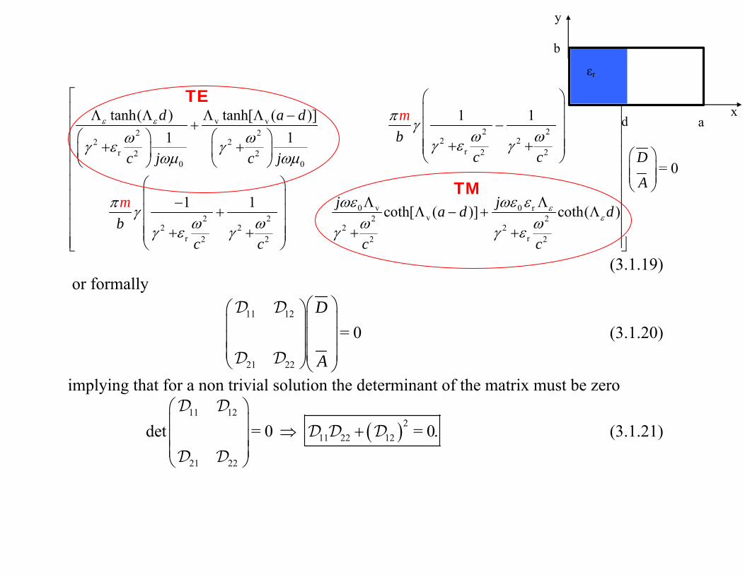
v v2 22 2
2 22 2r 2 2r 2 2
0 0
0 v 0 rv2 2 2 2
2 2 2 2r r2 2 2 2
tanh( ) tanh[ ( )] 1 11 1
1 1 coth[ ( )] coth( )
d a db
c cc j c j
j ja d db
c c
m
c
m
c
ε ε
εε
π γω ωω ω γ ε γγ ε γ
ωμ ωμ
ωε ωε επ γω ω ω ωγ ε γ γ γ ε
⎡ ⎛ ⎞⎢ ⎜ ⎟Λ Λ Λ Λ −
+ −⎢ ⎜ ⎟⎛ ⎞ ⎛ ⎞⎢ ⎜ ⎟+ ++ + ⎜ ⎟⎜ ⎟ ⎜ ⎟⎢ ⎝ ⎠⎝ ⎠ ⎝ ⎠⎢⎢ ⎛ ⎞⎢ ⎜ ⎟ Λ Λ−
+ Λ − + Λ⎢ ⎜ ⎟⎢ ⎜ ⎟+ + + +⎜ ⎟
⎝ ⎠⎣
= 0D
A
⎤⎥⎥⎥⎥⎛ ⎞⎥⎜ ⎟⎜ ⎟⎥⎝ ⎠⎥⎥⎥
⎢ ⎥⎦ (3.1.19) or formally
11 12
21 22
= 0D
A
⎛ ⎞⎛ ⎞⎜ ⎟⎜ ⎟⎜ ⎟⎜ ⎟
⎜ ⎟⎜ ⎟⎝ ⎠⎝ ⎠
D D
D D (3.1.20)
implying that for a non trivial solution the determinant of the matrix must be zero
( )11 12
211 22 12
21 22
det = 0 = 0.⎛ ⎞⎜ ⎟ ⇒ +⎜ ⎟⎜ ⎟⎝ ⎠
D DD D D
D D (3.1.21)
x
y
a
b
d
εr
TE
TM

x
y
a
b
d
εr
Comments: 1. The diagonal terms represent the dispersion relation of TE and
TM modes. 2. If there are no variations in one transverse dimension (e.g. = 0m ), the TE and
TM modes are decoupled. Such an example will be considered in the next section.
Exercise 3.1: Analyze the solution of the dispersion relation as a function of d . Specifically, compare to the case = 0d and =d a . Exercise 3.2: Calculate the group velocity and the energy velocity. Exercise 3.3: For a given propagating power, determine the ratio of electric and magnetic energy (per unit length) as a function of d .

3.2 Dielectric Loading – TM01
In the previous section it was concluded that partial
loading in one direction and the field variations in the other direction leads to hybrid modes. Moreover, we claimed that if there are no field variations in the second transverse direction the modes are not coupled. We shall examine this kind of configuration next, namely, a partially filled with dielectric rε configuration as illustrated in Figure 2. The radius of the waveguide is R and the inner radius of the dielectric is denoted with
dR . We shall assume a solution of the form ( )( , ) = ( )expzE r z E r jkz− in which case the amplitude ( )E r
satisfies
( )2
2r2
1 ( ) = 0d dr r k E rr dr dr c
ω ε⎡ ⎤
+ −⎢ ⎥⎣ ⎦
(3.2.1)
Rd R

in the dielectric region or explicitly for < <dR r R :
2
212
2
1 ( ) = 0d dr k E rr dr dr c
κε
ω ε
⎡ ⎤⎢ ⎥
+ −⎢ ⎥⎢ ⎥⎢ ⎥⎣ ⎦
(3.2.2)
whereas in the vacuum 0 < < dr R :
2
222
2v
1 ( ) = 0.d dr k E rr dr dr c
κ
ω⎡ ⎤⎢ ⎥
+ −⎢ ⎥⎢ ⎥⎢ ⎥⎣ ⎦
(3.2.3)
It is therefore convenient to define the radial wave number ( )22 2v / c kκ ω≡ − in vacuum
(subscript v) whereas the corresponding quantity in the dielectric is defined as ( )22 2/ c kεκ ε ω≡ − based on which the solution reads
Rd R

( ) 0
0
20 0
0 20 0 0 0
20 v v
0 20 v v
( ) 0 < <( ) < <
( ) ( ) ( ) ( ) > 0( )
(| | ) (| | ) (| | ) (| | ) 0
( ) > 0( ) =
(| | ) 0
dz
d
o o
AS r r RE r
BT r R r R
J r Y R Y r J RT r
I r K R K r I R
J rS r
I r
ε ε ε ε ε
ε ε ε ε ε
κ κ κ κ κκ κ κ κ κ
κ κκ κ
⎧= ⎨⎩⎧ −
≡ ⎨− <⎩
⎧⎨
<⎩
(3.2.4)
As in the previous section the dispersion relation will be now determined by imposing the boundary conditions at the interface between the two regions. Firstly, we impose the continuity of zE at = dr R :
0 0( ) = ( )z d dE AS R BT R⇒ (3.2.5) and secondly, the continuity of Hϕ at = dr R
( )0 v
0 02 2 22v
| | | |= ( ) = ( )/r z
r d dr
j EH BT R AS Rrk c
εϕ
ε
ωε ε κ κεκ κε ω
∂⇒
∂− (3.2.6)
wherein
Satisfies the boundary condition on the external wall
Satisfies the boundary condition in the center
Rd R

21 1 0
0 21 0 1 0
21 v v
0 21 v v
( ) ( ) ( ) ( ) > 0( )
(| | ) (| | ) (| | ) (| | ) 0
( ) > 0( ) =
(| | ) 0
oJ r Y R Y r J RT r
I r K R K r I R
J rS r
I r
ε ε ε ε ε
ε ε ε ε ε
κ κ κ κ κκ κ κ κ κ
κ κκ κ
⎧− +≡ ⎨
+ <⎩⎧ −⎨
<⎩
(3.2.7)
From the previous two equations[(3.2.5), (3.2.6)] we obtain the dispersion equation
v0 00 02 2
v
| | | |=rS T S Tε
ε
κ κεκ κ
(3.2.8)
which can be solved numerically as illustrated below. According to the frequency, the mode varies from the characteristics of empty space (close to cut-off) of dielectric filled case.
Rd R
0 1 2 3 4 5 60
5
10
15
20
kR
[] z
GH
fempty waveguide
waveguidedielectric filled

Exercise 3.4: Analyse the effect of dR on the phase velocity, group velocity and ohm loss of the metal. What about dielectric loss? Exercise 3.5: Analyze the ratio of the electric energy stored per unit length vs. magnetic energy per unit length. Exercise 3.6: Compare the energy stored in the dielectric with that in air. Exercise 3.7: Determine the higher modes of a coaxial line illustrated below. The radii are in d ext, ,R R R .
R
airmetal
dielectric

3.3 Mode Coupling 3.3.1 Step Transition – TE mode
A longitudinal change in the cross-section of the waveguide leads to a coupling
process between virtually all possible modes. Excitation of modes is an inherent process associated with the necessity to satisfy the boundary conditions. Whether these modes propagate or not, it is only a question of what is the frequency (or frequencies) of the incoming signal. In general, the coupling occurs between TE and TM or between various hybrid modes however, in what follows we shall consider a configuration whereby the coupling is between the various eigen-modes of a TE mode.

x
y
z
z=0
a
b
d
a d
z=0 x z
A TE01 wave propagates from z → −∞ towards the discontinuity at = 0z
( )(inc)0 z= cos expz
xH H jk za
π⎛ ⎞⎜ ⎟⎝ ⎠
(3.3.1)
in a waveguide of width a and height b ; note that ( ) ( )2 22 / /zk c aω π= − . At the discontinuity the width of the waveguide varies abruptly from a to <d a . A direct result of the discontinuity is a reflected field described by
( ) ( ) ( )2 2(ref )0
=0
= cos exp ; = / /z n n mn
nxH H z m a ca
πρ π ω∞ ⎛ ⎞ Γ Γ −⎜ ⎟
⎝ ⎠∑ (3.3.2)

mρ are the reflection coefficients of the various modes. Similarly, the transmitted field is given by
( ) ( ) ( )2 2(tr )0
=0
= cos exp ; = / /z m m mm
mxH H z m d cd
πτ π ω∞ ⎛ ⎞ −Λ Λ −⎜ ⎟
⎝ ⎠∑ (3.3.3)
mτ representing the transmitted coefficient of each mode. Three observations at this stage:
1. The amplitude of both reflected ( )mρ and transmitted ( )mτ will be determined by the boundary conditions to be imposed shortly.
2. The character of the mode (propagating or evanescent) is determined by the angular frequency ( )ω of the incident wave.
3. The choice of TE01 is dictated by the need for a simple analysis. If a higher mode is launched (e.g. TE11 ) there will be coupling to TM modes.
a d
z=0 x z

Step 1: Continuity of the y -component of the electric field in the range 0 < <x a implies
( tr )
(inc) (sc) =0=0
| 0 < <( | =
0 < < .y z
y y zE x d
E Ed x a
⎧+ ⎨
⎩ (3.3.4)
Faraday's law, in our case 0=x y zE j Hωμ∂ − , thus
( )=0 0
(sc)=0 0
( )=0 0
| = sin
| = sin
| = sin .
incy z o
y z o mm
try z o m
m
a xE j Ha
a mxE j Hm ad m xE j Hm d
πωμπ
πωμ ρπ
πωμ τπ′
′
⎛ ⎞ ⎛ ⎞− ⎜ ⎟ ⎜ ⎟⎝ ⎠ ⎝ ⎠
⎛ ⎞ ⎛ ⎞− ⎜ ⎟ ⎜ ⎟⎝ ⎠ ⎝ ⎠
′⎛ ⎞ ⎛ ⎞− ⎜ ⎟ ⎜ ⎟′⎝ ⎠ ⎝ ⎠
∑
∑ (3.3.5)
Substituting in (3.3.4) we get
,1
sin 0 < <[ ]sin =
0 < < .
mmm m
m
d m x x da mxm d
m ad x a
πτπδ ρ ππ
′′
′⎧ ⎛ ⎞⎪⎛ ⎞ ⎜ ⎟′+ ⎝ ⎠⎨⎜ ⎟
⎝ ⎠ ⎪⎩
∑∑ (3.3.6)
Using the orthogonality of the trigonometric function we obtain
a d
z=0 x z

,1 0
1 1[ ] = sin sin ,2
d
m m mm
a d m x mxdxm m a d a
π πδ ρ τπ π ′
′
′⎛ ⎞ ⎛ ⎞+ ⎜ ⎟ ⎜ ⎟′ ⎝ ⎠ ⎝ ⎠∑ ∫ (3.3.7)
or ,1 = ,m m mm m
m
Aδ ρ τ′ ′′
+ ∑ (3.3.8)
wherein the matrix mmA ′ is proportional to the overlap integral of the modes from both sides of the discontinuity
2
0ssi in12 n .
d
mmd mA d m x ma
xa
xm d d
π π′
′⎛⎛ ⎞ ⎛ ⎞≡ ⎜ ⎟ ⎜ ⎟′⎝ ⎠ ⎝ ⎠⎛ ⎞⎜ ⎟⎝
⎜ ⎟⎝ ⎠ ⎠
⎞∫ (3.3.9)
Step 2: Continuity of the x -component of the magnetic field in the region 0 < <x d implies
( ) ( ) ( )=0 =0| = |inc sc tr
x x z x zH H H+ (3.3.10) and since = 0H∇⋅ or explicitly = 0z z x xH H∂ + ∂ we get at = 0z
a d
z=0 x z

( )(inc)0 z01
(sc)0
( tr )0
= sin
= sin
= sin ( ).
x
x m mm
x m mm
a xH H jka
a mxH Hm ad m xH Hm d
ππ
πρπ
πτπ′′
⎛ ⎞− −⎜ ⎟⎝ ⎠
⎛ ⎞− Γ⎜ ⎟⎝ ⎠
′⎛ ⎞− −Λ⎜ ⎟′ ⎝ ⎠
∑
∑ (3.3.11)
Thus, in the region 0z = and 0 < <x d
0 ,1[ ]sin = sin ;m m m om mm
a mx d m xm a m d
π πδ ρ τπ π ′ ′
′
′⎛ ⎞ ⎛ ⎞Γ − + − Λ⎜ ⎟ ⎜ ⎟′⎝ ⎠ ⎝ ⎠∑ ∑ (3.3.12)
this time we use the orthogonality of ( )sin /m x dπ ′ in the range 0 x d≤ ≤ we get
,1 0
1 1= sin sin ,2
d
m m m m mm
d a m mdx x xm m d d a
π πτ δ ρπ π′ ′
′⎡ ⎤ ⎡ ⎤ ⎛ ⎞ ⎛ ⎞⎡ ⎤Λ Γ − ⎜ ⎟ ⎜ ⎟⎣ ⎦⎢ ⎥ ⎢ ⎥′⎣ ⎦ ⎣ ⎦ ⎝ ⎠ ⎝ ⎠∑ ∫ (3.3.13)
or ,1= [ ],m m m m m
mBτ δ ρ′ ′ −∑ (3.3.14)
where the matrix m mB ′ is also proportional to the overlap integral
a d
z=0 x z

0
sin12 .sind
mm m
m
a mB dxd m d
m xa
xd
mπ π′
′
′′ Γ≡
Λ⎛ ⎞⎜ ⎟⎝
⎛ ⎞⎟
⎝ ⎠ ⎠⎜∫ (3.3.15)
We can now write (3.3.8) and (3.3.14) in a vector form = and = ( )A Bδ ρ τ τ δ ρ+ − (3.3.16)
respectively. Substituting the expression for τ we obtain = ( )ABδ ρ δ ρ+ − , or [ ] = [ ]I AB AB Iρ δ+ − . Finally the amplitudes of the reflected and transmitted amplitudes are given by
1
1
= [ ] [ ]
= 2[ ] .
I AB AB I
I BA
ρ δ
τ δ
−
−
+ −
+ (3.3.17)
For evaluation of the matrices A and B we need to evaluate the integral
0
1 sin sin = sinc sinc .′ ⎡ ⎤ ⎡ ⎤⎛ ⎞ ⎛ ⎞ ⎛ ⎞ ⎛ ⎞′ ′− − +⎜ ⎟ ⎜ ⎟ ⎜ ⎟ ⎜ ⎟⎢ ⎥ ⎢ ⎥⎝ ⎠ ⎝ ⎠ ⎝ ⎠ ⎝ ⎠⎣ ⎦ ⎣ ⎦∫
d m x mx d ddx m m m md d a a a
π π π π (3.3.18)
a d
z=0 x z

With the amplitudes established we may proceed and evaluate the power in the system:
22 2
inc 0 ,1 0=1
22 2
ref 0 0=1
22 2
tr 0 0=1
1= | | Re( )2 2
1= | | Re( )2 2
1= | | Re( )2 2
m mm
m mm
m mm
a aP H b jm
a aP H b jm
d dP H b jm
δ ωμπ
ρ ωμπ
τ ωμπ
∞
∞
∞
′
⎛ ⎞ − Γ⎜ ⎟⎝ ⎠
⎛ ⎞ Γ⎜ ⎟⎝ ⎠
⎛ ⎞ − Λ⎜ ⎟′⎝ ⎠
∑
∑
∑ (3.3.19)
Assuming that at the operating frequency there is only a single propagating mode in each region, then the average power may be written as in a transmission line
2 1inc 1 1 1 0 1 0
1
2 2ref 1 1 1
2 2 2tr 2 1 2 2 0 2 0
2
1= | | = , =2 21= | | | |21= | | | | = , =2 2
k a abP I Z Z I Hck
P I Z
k d dbP I Z Z I Hck
ωηπ
ρ
ωτ ηπ
⇒
⇒ (3.3.20)
a d
z=0 x z

wherein ( ) ( )2 21 = / /k c aω π− and ( ) ( )2 2
2 = / /k c dω π− . Let us examine closely the normalized reflected power ( ) ( )ref inc
1 1/P P⎡ ⎤⎣ ⎦ in the first mode as a function of the
frequency: 1. The power can be injected at frequencies
above 6GHz (a=2.5cm). 2. To the point whereby the first mode in the
second part is above cutoff 8.485cf GHz ( = / 2d a )
the reflection coefficient of the first mode is unity. 3. Above 8.485GHz power can be transferred to the second part therefore the
reflected power drops yet ( ) ( ) ( )inc ref tr1 1 1=P P P+ .
4. Above 12 GHz for which the second mode in the left-hand side may carry power, the power reflected in the first mode decreases further yet beyond this point ( ) ( ) ( )inc ref tr
1 1 1P P P≠ + but rather ( ) ( ) ( ) ( )inc ref ref tr1 1 2 1P P P P= + + .
4 6 8 10 12 14 16 180.4
0.6
0.8
1.0
1.2
Ref
lect
ion
coef
ficie
nt
[ ]zGHf

3.3.2 Step Transition – TM0n Mode in Cylindrical Waveguide
An additional example illustrating mode-coupling due to discontinuity in the transverse geometry is brought next. In fact, in this case there are two discontinuities, and the first and last sections have the same cross section. It will be reiterated that even if the incident wave is composed of a single (lowest) mode, the coupling causes other modes that in turn may carry part of the electromagnetic energy.
In the left hand side ( < 0z ) of a cylindrical waveguide of radius extR , there is an incident and a reflected TM wave
( )
( )
(inc)0 0 1 1
ext
(ref )0 0 1
=1 ext
( , ) = exp
( , ) = exp ,
z
z s ss
rE r z E J p zR
rE r z E J p zR
ρ∞
⎛ ⎞−Γ⎜ ⎟
⎝ ⎠⎛ ⎞
Γ⎜ ⎟⎝ ⎠
∑ (3.3.21)
where 2 2ext( / ) ( / )s sp R cωΓ ≡ − and sρ represents the normalized amplitudes of the
Rext
Rint d
z z = 0

reflected modes. In the region 0 z d≤ ≤ the radius of the waveguide is smaller int ext<R R however for z d≥ the radius returns to its initial value. Consequently, in the other regions we have
( ) ( )
[ ]
( )0 0
=1 int
( tr )0 0
=1 ext
( , ) = exp exp
( , ) = exp (
dz n n n n n
n
z s s ss
rE r z d E J p A z B zR
rE r z d E J p z dR
τ
∞
∞
⎛ ⎞⎡ ⎤< −Λ + Λ⎜ ⎟ ⎣ ⎦
⎝ ⎠⎛ ⎞
> −Γ −⎜ ⎟⎝ ⎠
∑
∑ (3.3.22)
where 2 2int= ( / ) ( / )n np R cωΛ − . As previously, the goal is to determine the
amplitudes of the transmitted and reflected waves ( sτ and sρ ). For this purpose let us concentrate on the field components at = 0z .
( ) ( )( ) ( )
( ) ( )( ) ( )
(left ),1 10ext
0 1(left ),1 11 ext
(d)0int
0 1(d)int
exp exp=
exp exp
exp exp=
exp exp
s s ss
s s s ssr
n n n nn
n n n n n nnr
z zjH R rE J pz zp RE
j A z B zH R rE J pA z B zp RE
ϕ
ϕ
δ ρωεδ ρ
ωε
⎛ ⎞−Γ + Γ⎛ ⎞ ⎛ ⎞⎛ ⎞⎜ ⎟⎜ ⎟ ⎜ ⎟⎜ ⎟ −Γ − ΓΓ⎝ ⎠ ⎝ ⎠⎝ ⎠ ⎝ ⎠
⎛ ⎞−Λ + Λ⎛ ⎞ ⎛ ⎞⎛ ⎞⎜⎜ ⎟ ⎜ ⎟⎜ ⎟Λ −Λ − Λ⎝ ⎠ ⎝ ⎠⎝ ⎠ ⎝
∑
∑ ⎟⎠
(3.3.23)
With these field components we impose the boundary conditions at = 0z . Continuity of
Rext
Rint d
z z = 0

the radial electric field implies
int
int ext
( , = 0 ) 0 < <( , = 0 ) =
0 < <r
rE r z r R
E r zR r R
+− ⎧
⎨⎩
(3.3.24)
Using the orthogonality of the Bessel functions
ext2
2ext1 1 10
ext ext
= ( )2
R
s s s ssRr rdrrJ p J p J p
R Rδ′ ′
⎛ ⎞ ⎛ ⎞⎜ ⎟ ⎜ ⎟⎝ ⎠ ⎝ ⎠
∫ (3.3.25)
we obtain from (3.3.24) intint
,1 1 12 02 =1ext ext ext int
1
1= [ ]( )
2
R
s s n n n s nns n
ss
R r rA B drrJ p J pR R p R RJ pp
δ ρ∞ ⎛ ⎞ ⎛ ⎞
− Λ − ⎜ ⎟ ⎜ ⎟Γ ⎝ ⎠ ⎝ ⎠∑ ∫ (3.3.26)
or
,1=1
= [ ],s s sn n nn
A Bδ ρ∞
− −∑L (3.3.27)
where the matrix snL is proportional to the overlap integral int
3int
, ,2 3 2 01 ext i
1ex
1intt tn
1 2,( )
Rs n
s sn s n s nn s s
nrJ p
Rp R U U dr rp J p
JRR Rrp
⎛ ⎞Λ⎜ ⎟
⎛ ⎞⎜ ⎟
⎠ ⎠≡
Γ ⎝⎝≡ ∫L (3.3.28)
Rext
Rint d
z z = 0

The continuity of the azimuthal magnetic field in the region int0 < <r R is
( ) ( )( , = 0 ) = ( , = 0 )d dH r z H r zφ φ− + . Again we use the orthogonality of the
Bessel functions in the inner region int
22int int ext
1 ,1 1 10=1 ext int
[ ] ( ) = [ ]2
R
n n n s s s nsn s
R R R r rA B J p drrJ p J pp p R R
δ ρ∞ ⎛ ⎞ ⎛ ⎞
+ + ⎜ ⎟ ⎜ ⎟⎝ ⎠ ⎝ ⎠
∑ ∫ (3.3.29)
hence ,1= ( ),n n ns s s
sA B δ ρ+ +∑M (3.3.30)
where using the definition (3.3.28) we have further defined
ext,2
int 1
1 .( )
nsn s n
s n
R p UR p J p
≡M (3.3.31)
From these expressions we can easily deduce the two equations representing the boundary conditions at =z d :
( ) ( )=1
exp exp =n n n n ns ss
A d B d τ∞
−Λ + Λ ∑M (3.3.32)
Rext
Rint d
z z = 0

( ) ( ),=1
= [ exp exp ].s s n n n n nn
A d B dτ∞
−Λ − Λ∑L (3.3.33)
All four equations (3.3.27), (3.3.30), (3.3.32), (3.3.33) can be formulated in a vector (matrix) notation
( ) ( )( ) ( )( )( ) ( )
1 1 1
1 1 1 1
3.3.273.3.30
3.3.32 003.3.33 0
d d d
d d d
A B A I IA B B I I
Ae Be A I IeB I IAe Be e
δ ρ δδ ρ ρ
τ ττ
− − −
−−Λ Λ −−Λ − −
−Λ Λ Λ
⎫→ − = − − ⎛ ⎞−⎛ ⎞ ⎛ ⎞ ⎛ ⎞⇒ =⎬ ⎜ ⎟⎜ ⎟ ⎜ ⎟ ⎜ ⎟→ + = + ⎝ ⎠ ⎝ ⎠ ⎝ ⎠⎝ ⎠⎭⎫→ + = −⎛ ⎞ ⎛ ⎞−⎛ ⎞ ⎛ ⎞ ⎛ ⎞⎪⇒ =⎬ ⎜ ⎟ ⎜ ⎟⎜ ⎟ ⎜ ⎟ ⎜ ⎟→ − = ⎝ ⎠ ⎝ ⎠ ⎝ ⎠⎝ ⎠ ⎝ ⎠⎪⎭
L L LM M M
M L LL M M
(3.3.34) Substituing we get
Rext
Rint d
z z = 0

1 1 1 11 1
1 1 11 1 1
10
00or
00 0
d
d
d
d
I I I II I I I
I I I II
ee
eeI I I
δ τρ
τ δρ
−−Λ
Λ
−Λ
Λ
− −−
− −
− − −
− − − −
⎛ ⎞⎛ ⎞ ⎛ ⎞= ⎜ ⎟⎜ ⎟ ⎜ ⎟
⎝ ⎠ ⎝ ⎠⎝ ⎠
⎛ ⎞⎛ ⎞ ⎛ ⎞= ⎜ ⎟⎜ ⎟ ⎜ ⎟
⎝ ⎠ ⎝ ⎠⎝ ⎠
⎛ ⎞ ⎛ ⎞− −⎜ ⎟
− −⎛ ⎞ ⎛ ⎞⎜ ⎟ ⎜ ⎟⎝ ⎠ ⎝ ⎠
− −⎛ ⎞ ⎛ ⎞⎜ ⎟ ⎜ ⎟⎝ ⎠ ⎝
⎜ ⎟⎝ ⎠ ⎝ ⎠
⎛ ⎞ ⎛ ⎞− −⎜ ⎟ ⎜ ⎟⎝ ⎠ ⎠⎠ ⎝
L L L LM M M M
L L L LM M M M
(3.3.35)
or using a short notation
11 12
21 22
=0
Q QQ Q
δ τρ
⎛ ⎞⎛ ⎞ ⎛ ⎞⎜ ⎟⎜ ⎟ ⎜ ⎟
⎝ ⎠ ⎝ ⎠⎝ ⎠ (3.3.36)
thus 11 12 =Q Qδ ρ τ+ and 21 22 = 0Q Qδ ρ+ . Consequently, 1 1
22 21 11 12 22 21= , = [ ] .Q Q Q Q Q Qρ δ τ δ− −− − (3.3.37) The Figure below illustrates the reflection coefficient and power conservation as a function of the frequency. We observe that below the cut-off of the second mode all the propagating power is in the first mode. As the frequencies exceed the cut-off of the second mode, part of the power leaves the system through the second mode.
Rext
Rint d
z z = 0

The reflection coefficient as a function of the frequency and energy conservation of the first mode. Note that as long as the higher mode is below cutoff, 2 2
1,11,1| | | | = 1ρ τ+ while above cutoff, energy is transferred from the
first mode to the second and therefore 2 21,11,1| | | | 1ρ τ+ ≠ .
5 10 15 200.5
0.6
0.7
0.8
0.9
[ ]zGHf
11ρ
0.8
0.9
1.0
1.1
211
211
τρ
+
5 10 15 20
[ ]zGHf

3.4 Reactive Elements Obstacles in waveguides or transmission lines may cause reflections which in turn
may be detrimental. Power reflected implies obviously reduction in the transmitted power but it entails that some energy is stored in the evanescent waves which develop in the vicinity of the obstacle.
3.4.1 Inductive Post
As an example we shall examine a cylindrical post and an incident TE01 mode determined by
( ) ( ) 2 20 1 1( , ) = sin exp ; = ( / ) ( / ) =p
yxE x z E z a c ja
π π ω β⎛ ⎞ −Γ Γ −⎜ ⎟⎝ ⎠
(3.4.1)
In zero order this primary field excites in the metallic cylinder a current density
( , ) = ( ) ( )yJ x z I z x dδ δ − (3.4.2) which may be interpreted as surface current density
x a
b
d
y
2R

,=1
( ) = ( ) = sin∞ ⎛ ⎞− ⎜ ⎟
⎝ ⎠∑y s mm
xJ x I x d U ma
δ π (3.4.3)
hence
2= sin .⎛ ⎞⎜ ⎟⎝ ⎠
mdU I m
a aπ (3.4.4)
This current generates a secondary field
( )(sec)
=1( , ) = sin expy m m
m
xE x z m za
π∞ ⎛ ⎞ −Γ⎜ ⎟
⎝ ⎠∑E (3.4.5)
where 2 2 2 2= ( / ) /m m a cπ ωΓ − . In order to establish the relation between the current's ``harmonics'' and the secondary field we observe that based on Maxwell's equations the magnetic field
( )(sec)
=10
1( , ) = sin exp sgn( )x m m mm
xH x z m z zj a
πωμ
∞− ⎛ ⎞Γ −Γ⎜ ⎟⎝ ⎠
∑ E (3.4.6)
enables via its discontinuity condition ,( , = 0 ) ( , = 0 ) =x x y sH x z H x z J+ −− (3.4.7)
to determine the amplitudes of the modes describing the secondary field in terms of the current on the filament

0= sin .⎛ ⎞− ⎜ ⎟ Γ⎝ ⎠m
m
jI dma a
ωμπE (3.4.8)
We have yet to determine the relation between the current ( )I in the filament and the amplitude of the incident wave. This is done by relaxing the condition of our infinitely small filament and imposing that the tangential electric field vanishes on the wall of the post. Specifically, averaging the electric field over the azimuthal coordinate at =r R we must get zero total field, namely
2 ( ) (sec)
= cos0= sin
[ ] = 0.incy y x d R
z R
d E Eπ
φφ
φ ++∫ (3.4.9)
explicitly
( ) ( ) ( )2
0 ,10=1
exp sin exp sin sin cosm m m mm
md E R R d Ra
π πφ δ φ φ φ∞ ⎡ ⎤⎡ ⎤−Γ + −Γ +⎢ ⎥⎣ ⎦ ⎣ ⎦∑∫ E (3.4.10)
which formally may be rewritten by defining
( ) ( )2(1)
0
1 exp sin sin cos2m m
md R d Ra
π πφ φ φπ
⎡ ⎤≡ −Γ +⎢ ⎥⎣ ⎦∫L (3.4.11)
and
( ) ( )2(2)
0
1 exp sin sin cos2m m
md R d Ra
π πφ φ φπ
⎡ ⎤≡ −Γ +⎢ ⎥⎣ ⎦∫L (3.4.12)
x a
b
d
y
2R

hence
( ) ( )
(1)(1) (2)0 01
0 1(2)=1 0
=1
1 sin = 0 = ./ sin /
mm m
m mm
j E adE I m Ia a j c md a
ωμπηω π
∞
∞⎛ ⎞− ⇒⎜ ⎟ Γ⎝ ⎠ Γ
∑∑
LL L
L
(3.4.13) At this stage we may define the reflection coefficient
( ) ( )
( ) ( )
(1)1
(2)0
=1
/ sin /=
/ sin /
mmm
n nn
j c md aE j c nd a
ω πρ
ω π∞
− Γ≡
Γ∑LE
L (3.4.14)
or for the fundamental ( ) ( )
( ) ( ) ( ) ( )
(1)1
1(2) (2)1
=2
/ sin /= .
/ sin / / sin /n nn
c d a
c d a j c nd a
ω β πρ
ω β π ω π∞
−
+ Γ∑L
L L (3.4.15)
At this point it can be shown that since = 1m is a propagating mode (1) (2)1 1= Re( )L L and
the second term in the denominator is pure imaginary
( )( )
1 (2)(2)1
(1) (1)=21 1
1= .sin /Im( )1sin /
n
n n
nd aj j
d a
ρπβπ
∞
−⎛ ⎞
+ + ⎜ ⎟Γ⎝ ⎠∑LL
L L
(3.4.16)
x a
b
d
y
2R

Based on this last result, we conclude that the post may be represented by a reactance since according to the equivalent scheme below
11 1= =
1 2 1 2L LZ j Xρ − −
+ +
and ( )( )
(2)(2)1
(1) (1)=21 1
sin /1 Im[ ]= .2 sin /
nL
n n
nd aX
d aπβπ
∞
+Γ∑LL
L L
Further simplification, is achieved assuming that R d we get
( ) ( )(1)0
1sin exp sin sin2m m m
d dm d R m I Ra a
π
ππ φ φ π
π −
⎛ ⎞ ⎛ ⎞−Γ Γ⎜ ⎟ ⎜ ⎟⎝ ⎠ ⎝ ⎠∫L (3.4.17)
( )
( ) ( ) ( )
(2)
0
01
2sin exp sin2
1sin 2 1 sinc2
m m
km k m
k
dm d Radm I R k I Ra
ππ φ φ
π
π π∞
=
⎛ ⎞ −Γ⎜ ⎟⎝ ⎠
⎡ ⎤⎛ ⎞ ⎛ ⎞Γ + − Γ⎜ ⎟ ⎜ ⎟⎢ ⎥⎝ ⎠ ⎝ ⎠⎣ ⎦
∫
∑
L
(3.4.18)
thus
x a
b
d
y
2R
ZL Z0 Z0

( ) ( ) ( )
( )
20 2 1
=2 0
20
14 sin2 1
=sin
kn k n
n kn nL
I R I R dnR k R a
XJ R d
R a
ππ
βπ
β
∞ ∞+
=
⎡ ⎤Γ Γ− ⎛ ⎞−⎢ ⎥ ⎜ ⎟Γ + Γ ⎝ ⎠⎢ ⎥⎣ ⎦⎛ ⎞⎜ ⎟⎝ ⎠
∑ ∑ (3.4.19)
At the limit 0R → or more precisely assuming 1 and 1nR Rβ Γ thus ( ) ( )1 / 2 / !I x x ν
ν ν we get
( ) ( )( )
1In 2 2 12
=2 0
t
2
11 4 1 sin2 1 2 1 ! 2
=1 sin
aR kk k
n
n knL
R dnR k k a
Xd
R a
π
ππ
πβ
⎛ ⎞⎜ ⎟⎝ ⎠ +∞
=
⎡ ⎤Γ− ⎛ ⎞ ⎛ ⎞−⎢ ⎥⎜ ⎟ ⎜ ⎟Γ + + ⎝ ⎠ ⎝ ⎠⎢ ⎥⎣ ⎦⎛ ⎞⎜ ⎟⎝ ⎠
∑ ∑ (3.4.20)

Exercise 3.8: Analyze (numerically) the dependence of the normalized reactance on three parameters; the angular frequency ( )ω , its location ( )d and its radius ( )R . It is possible to simplify the two quantities defined in (3.4.11) and (3.4.12) by using
=
1exp = ( ) ; ( ) = ( 1) ( ).2
k kk k k
k
z t t J z J z J zt
∞
−−∞
⎡ ⎤⎛ ⎞− −⎜ ⎟⎢ ⎥⎝ ⎠⎣ ⎦∑
(For solution see Appendix 10.1) Exercise 3.9: Calculate the energy stored in the vicinity of the post and compare it with energy per unit length carried by the incident wave. Exercise 3.10: Analyze the ratio of electric to magnetic energy stored around the post.

3.4.2 Diaphragm Another element (obstacle)
that may deflect radiation but not absorb it is the diaphragm. This is a thin metallic layer occupying part of the cross-section. Consider a diaphragm occupying the region
< <d x a its thickness being negligible compared to the wavelength and the skin depth. The electric field is given by
( ) ( ) ( )
( )
1=2
0
1=2
exp exp sin exp sin < 0=
sin exp sin > 0.
m mm
y
m mm
x xj z j z z m za a
E Ex xj ze z m za a
β ρ β π ρ π
βτ π τ π
∞
∞
⎧ ⎛ ⎞ ⎛ ⎞⎡ ⎤− + + Γ⎜ ⎟ ⎜ ⎟⎪⎣ ⎦⎪ ⎝ ⎠ ⎝ ⎠⎨
⎛ ⎞ ⎛ ⎞−⎪ + −Γ⎜ ⎟ ⎜ ⎟⎪ ⎝ ⎠ ⎝ ⎠⎩
∑
∑
(3.4.21) Let us denote by ( ) 0, 0 ( )yE x z E x= = E the transverse electric field in the aperture, thus
x a
b
d
y

1 1 0
2= 1: 1 = = ( )sin ⎛ ⎞+ ⎜ ⎟⎝ ⎠∫
d xm dx xa a
ρ τ πE (3.4.22)
0
22 : = = ( )sin .⎛ ⎞≥ ⎜ ⎟⎝ ⎠∫
d
m mxm dx x m
a aρ τ πE (3.4.23)
( )xE represents the horizontal variation of the vertical electric field ( )yE . Continuity of
xH in the aperture (0 < < )x d implies
1 1=2 =2
(1 )sin sin = sin sin .∞ ∞⎛ ⎞ ⎛ ⎞ ⎛ ⎞ ⎛ ⎞− − + Γ − − Γ⎜ ⎟ ⎜ ⎟ ⎜ ⎟ ⎜ ⎟
⎝ ⎠ ⎝ ⎠ ⎝ ⎠ ⎝ ⎠∑ ∑m m m mm m
x x x xj m j ma a a a
β ρ π ρ π βτ π τ π
(3.4.24) Substituting (3.4.23) we get
1 0=2
42 sin = sin ( )sin∞ ′Γ⎛ ⎞⎛ ⎞ ⎛ ⎞ ⎛ ⎞′ ′− −⎜ ⎟ ⎜ ⎟ ⎜ ⎟⎜ ⎟−⎝ ⎠ ⎝ ⎠ ⎝ ⎠⎝ ⎠∑ ∫
dm
m
x x xm dx x ma j a a a
ρ π π πβ
E (3.4.25)
and further multiplying and deviding by 11 ρ+ and using (3.4.22) we finally obtain
10 0
=21
2 'sin ( )sin = 2 sin ( )sin .1
d dm
m
x x x xdx x j m dx x ma a a a
ρ π π π πρ β
∞ ′⎛ ⎞Γ⎛ ⎞ ⎛ ⎞ ⎛ ⎞ ⎛ ⎞′ ′ ′ ′⎜ ⎟ ⎜ ⎟ ⎜ ⎟ ⎜ ⎟⎜ ⎟+ ⎝ ⎠ ⎝ ⎠ ⎝ ⎠ ⎝ ⎠⎝ ⎠∑∫ ∫E E
(3.4.26)
x a
b
d
y

Since the admittance is 1
1
2=1
LY ρρ
−+
in the left hand side may be rewritten
0 0=2
'sin ( )sin = 2 sin ( )sin .d dm
Lm
x x x xY dx x j m dx x ma a a a
π π π πβ
∞ ′⎛ ⎞Γ⎛ ⎞ ⎛ ⎞ ⎛ ⎞ ⎛ ⎞′ ′ ′ ′−⎜ ⎟ ⎜ ⎟ ⎜ ⎟ ⎜ ⎟⎜ ⎟⎝ ⎠ ⎝ ⎠ ⎝ ⎠ ⎝ ⎠⎝ ⎠
∑∫ ∫E E (3.4.27)
So far the formulation is exact (of course subject to the specified assumptions). At this stage we multiply both sides by ( )xE and integrate over the cross section of the aperture and get
2
0
2=2
0
( )sin= 2 .
'( )sin
d
mL
dm
xdx x maY j
xdx xa
π
βπ
∞
′⎡ ⎤⎛ ⎞′ ′ ⎜ ⎟⎢ ⎥⎛ ⎞Γ ⎝ ⎠⎣ ⎦− ⎜ ⎟⎝ ⎠ ⎡ ⎤⎛ ⎞′ ′ ⎜ ⎟⎢ ⎥⎝ ⎠⎣ ⎦
∫∑
∫
E
E
(3.4.28)
which evidently entails that the distribution of the electric field in the aperture determines the admittance of the diaphragm as experienced by the wave. For a rough approximation we may consider the simplest form of ( )xE that satisfies the boundary conditions at = 0x and =x d but it ignores edge effect namely, ( )( )x x d x∝ −E . An
estimate of the edge effect may be considered by ( )( )x x d x ν∝ −E with 0 1ν< ≤ .
x a
b
d
y

Exercise 3.11: Compare the admittace using the approximation ( )( )x x d x= −E with that evaluated by Lewin (Theory of Waveguides)
42= 1 sin .2
LdY j
a aπ πβ
−⎡ ⎤⎛ ⎞− ⎜ ⎟⎢ ⎥⎝ ⎠⎣ ⎦
Exercise 3.12: What is the effect of the edge of the diaphragm?
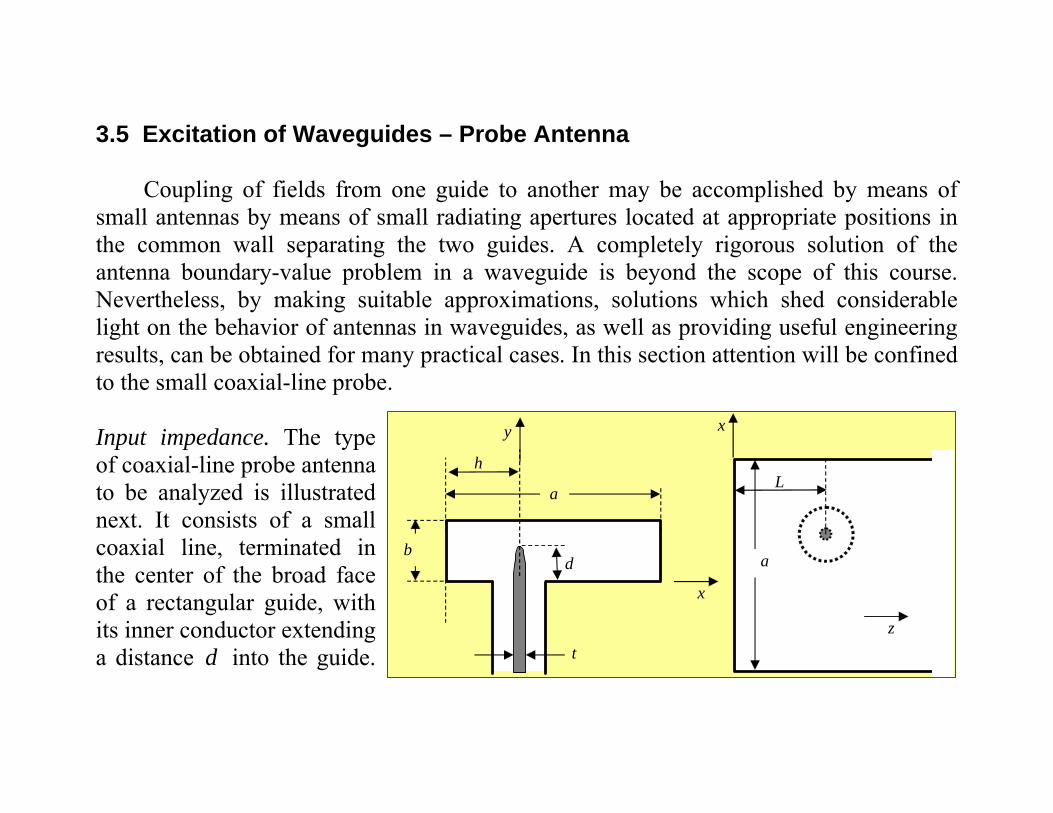
3.5 Excitation of Waveguides – Probe Antenna Coupling of fields from one guide to another may be accomplished by means of
small antennas by means of small radiating apertures located at appropriate positions in the common wall separating the two guides. A completely rigorous solution of the antenna boundary-value problem in a waveguide is beyond the scope of this course. Nevertheless, by making suitable approximations, solutions which shed considerable light on the behavior of antennas in waveguides, as well as providing useful engineering results, can be obtained for many practical cases. In this section attention will be confined to the small coaxial-line probe.
Input impedance. The type of coaxial-line probe antenna to be analyzed is illustrated next. It consists of a small coaxial line, terminated in the center of the broad face of a rectangular guide, with its inner conductor extending a distance d into the guide.
a
b
y
x
d
h
t
x
a
z
L

In order to have the antenna radiate in one direction only, a short-circuiting plunger is placed at a distance L to the left of the probe. The basic concept is to generate a current ( )I at a location where the parallel electric field is maximum -- quarter wavelength from a short circuiting plane.
b
y
z
L
2Rint
2Rext
The total field in the waveguide could be found if aE and aH , the total tangential
fields in the aperture were known. Unfortunately, these aperture fields are unknown, but, if the coaxial-line opening is small, we may, to a first approximation, assume that the higher-order coaxial-line modes which being excited, are negligible. The field in the aperture will then be that associated with the incident and reflected TEM modes in the coaxial line.

Relying on Poynting's complex theorem we find by denoting by P the power flow far away from the probe that
*1 = 2 [ ]2 y y M EdVJ E P j W Wω− + ⟨ ⟩ − ⟨ ⟩∫ (3.5.1)
where the current density may be approximated, assuming a thin probe, by
( )2 2int2
int
( )( , , ) = ( ) .yI yJ x y z u R x h z L
Rπ⎡ ⎤− − + −⎢ ⎥⎣ ⎦
(3.5.2)
This current density excites a TE nm mode satisfying
2 2
202 2
0
1=y y yE j J Jc j yω ωμ
ωε⎛ ⎞ ∂∇ + −⎜ ⎟ ∂⎝ ⎠
(3.5.3)
which in terms of Green's function reads
( ) ( )2 2
0 2 2( , , ) = ( , , | , , ) ', ', ' ', ', ' .'y y y y
cE x y z j dx dy dz G x y z x y z J x y z J x y zy
ωμω
⎡ ⎤∂′ ′ ′ ′ ′ ′− +⎢ ⎥∂⎣ ⎦∫
(3.5.4) In turn Green's function for our configuration is given by
b
y
z
L
2Rint
2Rext

( )
,0=1, =0
, ,
1( | ') = (1 )sin sin2
cos cos exp exp ( )
y mn m nm
n m n m
x xG r r n nab a a
y ym m z z z zb b
δ π π
π π
∞ ′⎛ ⎞ ⎛ ⎞+ ⎜ ⎟ ⎜ ⎟Γ ⎝ ⎠ ⎝ ⎠′⎛ ⎞ ⎛ ⎞ ′ ′⎡ ⎤ ⎡ ⎤× −Γ − − −Γ +⎜ ⎟ ⎜ ⎟ ⎣ ⎦ ⎣ ⎦⎝ ⎠ ⎝ ⎠
∑
(3.5.5) Exercise 3.13: Prove that this is the solution of
22
2 = ( ) ( ) ( )
( = 0, ) = 0, = 0, ( , , = 0) = 0.=0,
y
yy y
G x x y y z zc
GG x a G x y z
y y b
ω δ δ δ⎛ ⎞
′ ′ ′∇ + − − − −⎜ ⎟⎝ ⎠
∂
∂
Substituting (3.5.4) and (3.5.2) in (3.5.1) as well as taking advantage of the probe being thin we have
2 2*0
2 '2( ) ( | ) ( ) ( ) = 2 [ ]2 M E
j cdyI y dy g y y I y I y P j W Wy
ωμ ωω
⎡ ⎤∂′ ′ ′ ′+ + ⟨ ⟩ − ⟨ ⟩⎢ ⎥∂⎣ ⎦∫ ∫ (3.5.6)
wherein
b
y
z
L
2Rint
2Rext

( ) ( )
( )
,0=1 ,=0
2,
1( | ) = , , = | = , , = = (1 )2
sin 1 exp 2 cos cos
mn n mm
n m
g y y G x h y z L x h y z Lab
h y yn L m ma b b
δ
π π π
′ ′ ′ ′≡ +Γ
′⎛ ⎞ ⎛ ⎞ ⎛ ⎞⎡ ⎤× − − Γ⎜ ⎟ ⎜ ⎟ ⎜ ⎟⎣ ⎦⎝ ⎠ ⎝ ⎠ ⎝ ⎠
∑ (3.5.7)
In terms of the current at the aperture of the coax (interface coax-waveguide) the current is (0)I therefore, we may define the input impedance
2
2 [ ]1 | (0) |2
M Ein
P j W WZI
ω+ ⟨ ⟩ − ⟨ ⟩≡ (3.5.8)
hence 2 2*
0 2 '20 0( ) ( | ) ( ') ( ) .
d d
incZ j dyI y dy g y y I y I y
yωμ
ω⎡ ⎤∂′ ′ ′+⎢ ⎥∂⎣ ⎦
∫ ∫ (3.5.9)
At the end of the probe the current is zero, therefore, for simplicity sake we assume
2( )( ) = =
(0)I y y dI y
dI−⎛ ⎞
⎜ ⎟⎝ ⎠
(3.5.10)
or
b
y
z
L
2Rint
2Rext

2 2 2
in 0 2 20 0
2= ( | )d dy d y d cZ j dy dy g y y
d d dωμ
ω⎡ ⎤′− −⎛ ⎞ ⎛ ⎞′ ′ +⎢ ⎥⎜ ⎟ ⎜ ⎟
⎝ ⎠ ⎝ ⎠⎢ ⎥⎣ ⎦∫ ∫ (3.5.11)
Let us assume now that except the first mode, all the modes are evanescent. Clearly their contribution to the impedance is pure imaginary (inductive). Only the propagating mode has both imaginary and real contribution to the impedance
( ) ( ) ( )22
20in = sin sin sin cos 1 6
18d hZ L L j L dab c a c
η ω ωπ β β ββ
−⎡ ⎤⎛ ⎞ ⎛ ⎞⎡ ⎤+ +⎢ ⎥⎜ ⎟ ⎜ ⎟⎣ ⎦⎝ ⎠ ⎝ ⎠⎢ ⎥⎣ ⎦(3.5.12)
Comment: The required values of L and d to make = 0X and = cR Z , so that all the incident power is coupled into the guide, may be found graphically from a plot of the
= 0X and =R constant contours in the 0k d Lβ− plane. Such a plot is given in the
figure above for a guide of dimensions 2.3 1× cm and a probe diameter equal to 0.23cm at a wavelength of 3.14cm. The
b
y
z
L
2Rint
2Rext
4/π 2/π π 10β
0=X
Ω= 100RΩ= 70RΩ= 50R
dk0
4/3π1
2
3
L

intersection of the two curves determines the required parameters. From the figure it is seen that the self-resonant length of the antenna, corresponding to = 0Lβ or / 2π , is
00.28λ . Also it is seen that, for 0k d less than 1.22 ( < 0.61d centimeter), a value of Lβ which will make = 0X does not exist. The reason is that the TE10 mode standing wave between the antenna and the short-circuiting plunger cannot provide enough inductive reactance to counterbalance the high capacitive reactance of a short probe.

3.6 Coupling between Waveguides by Small Apertures Electromagnetic energy may be coupled from one waveguide into another guide or
into a cavity resonator by a small aperture located at a suitable position in the common wall. For apertures whose linear dimensions are small compared with the wavelength, an approximate theory is available which states that the aperture is equivalent to a combination of radiating electric and magnetic dipoles, whose dipole moments are respectively proportional to the normal electric field and tangential magnetic field of the incident wave. This theory was originally developed by H.A. Bethe in ``Theory of Diffraction by Small Holes", Physical Review, vol. 66, pp. 163--182, 1944.

3.7 Surface Waveguides In addition to the closed cylindrical conducting tube and the conventional TEM
wave-transmission line, there exists a class of open boundary structures which are capable of guiding an electromagnetic wave. The field is characterized by an exponential decay away from the surface and having the usual propagation function ( )exp j zβ− along the axis of the structure. Moreover it has a discrete spectrum of eigenmodes. This type of wave is called a surface wave, and the structure which guides this wave may be appropriately referred to as a surface waveguide. Some typical structures that are capable of supporting a surface wave are illustrated in Figure 10. These consist of dielectric-slabs, fibers, dielectric-coated planes and wires and corrugated planes and wires.
z
zz
z
(a) (b)
(c) (d)

Although surface waveguides have several features which are similar to those of the cylindrical conducting-tube guide, they have many characteristics which are quite different. Some of the outstanding differences are:
1. Propagation with no low-frequency cutoff. 2. Finite number of discrete modes of propagation at a given frequency. 3. Phase velocity smaller than that of plane wave in vacuum.
3.7.1 Dielectric Layer above a Metallic Surface Consider a TM mode and for the sake of simplicity, yet without significant loss of
generality, we shall examine the case when = 0y∂ , or more specifically TM01. This mode may be derived from the longitudinal electric field
rε
x
z
d
Basic configuration of the open dielectric waveguide.

( )
22
r2
22
2
sin 0 < <
( , ) = exp
exp ( ) >z
A x k x dc
E x z jkz
B x d k x dc
ω ε
ω
⎧ ⎛ ⎞⎪ −⎜ ⎟⎜ ⎟⎪⎪ ⎝ ⎠− ⎨
⎡ ⎤⎪− − −⎢ ⎥⎪⎢ ⎥⎪ ⎣ ⎦⎩
(3.7.1)
The x -component of the electric field may be derived using Gauss' law ( = 0)E∇⋅
( )
22
r222
r2
22
222
2
cos 0 < <
( , ) = exp
exp ( ) >x
jkA x k x dc
kcE x z jkzjkB x d k x d
ck
c
ω εω ε
ωω
⎧ ⎛ ⎞−⎪ −⎜ ⎟⎜ ⎟⎪ ⎝ ⎠−⎪⎪− ⎨
⎡ ⎤⎪ −− − −⎢ ⎥⎪⎢ ⎥⎣ ⎦⎪ −
⎪⎩
(3.7.2)
for establishing the magnetic field we use Ampere's law ( 0 r=H j Eωε ε∇× )
rε
x
z
d

( )
220 r
r 222
r 2
220
222
2
cos 0 < <
( , ) = exp
exp ( ) < < .y
j A x k x dc
kcH x z jkz
j B x d k d xc
kc
ωε ε ωεωε
ωε ωω
⎧ ⎡ ⎤−⎪ −⎢ ⎥⎪ ⎢ ⎥⎣ ⎦−⎪⎪− ⎨
⎡ ⎤⎪ −− − − ∞⎢ ⎥⎪⎢ ⎥⎣ ⎦⎪ −
⎪⎩
(3.7.3) Continuity of the tangential electric field implies
2
2r 2: sin =zE A d k B
cωε
⎡ ⎤−⎢ ⎥
⎢ ⎥⎣ ⎦ (3.7.4)
whereas the continuity of the tangential magnetic field
2
2rr 22 2
2 2r 2 2
1: cos = .yH A d k Bc
k kc c
ε ωεω ωε
⎡ ⎤−⎢ ⎥
⎢ ⎥⎣ ⎦− −
(3.7.5)
These two equations lead to the following dispersion relation
rε
x
z
d

2
22tan( ) = ,rd k
cωξ ξ ε − (3.7.6)
where 2
2rd k
cωξ ε≡ − . It is also convenient to define 0 r= 1d
cωξ ε − therefore, we
may write
2 2 2
2 2 2 2 2 2r 02 2 2= ( 1) =d k d k
c c cω ω ωξ ε ξ ξ
⎡ ⎤− + − ⇒ − −⎢ ⎥
⎣ ⎦ (3.7.7)
Consequently, the dispersion relation reads
2 2r 0tan( ) = .ξ ξ ε ξ ξ−
(3.7.8) The two sides of the equation are plotted in the figure below
rε
x
z
d
rε
x
z
d

Clearly for a single mode operation, we require
that 0r
1< <1c d
ω πξ πε
⇒−
.
We shall examine what happens at low frequencies i.e. 00, 0ξ ξ→ → . At this limit the dispersion relation reads
2 2 2r 0=ξ ε ξ ξ− (3.7.9)
The solution of the fourth order polynomial which corresponds to a low-frquency propagating wave is
2
2 2 2 02
1= 1 42 r r
r
ξξ ε εε
⎡ ⎤− + +⎢ ⎥⎢ ⎥⎣ ⎦
(3.7.10)
and now substituting the definitions of ξ and 0ξ we get
2
2eff= ⎛ ⎞⎜ ⎟⎝ ⎠
kcωε (3.7.11)
which is only weakly dependent on the thickness (provided d λ ) but is dependent on
rε
x
z
d
03ξε r
02ξε r
01ξε r
π2π
23π03ξ02ξ01ξ ξ
( )ξξ tan
( )ξξ tan

the dielectric coefficient (but > 1rε ). To be more accurate
( )
22 22
r r2 2 2
22
2
4= 1 1 12
=
r
r
k dc d c
kc
ω ε ωε εε
ω
⎡ ⎤⎛ ⎞⎢ ⎥− − + + −⎜ ⎟⎢ ⎥⎝ ⎠⎣ ⎦ (3.7.12)
where the effective dielectric coefficient is unity.
rε
x
z
d

The figure below illustrates the dispersion relation of the system.
rε
x
z
d
kd
dcω
dcω
rdcω ε3
0.5cmr
dε ==

Our next step is to examine the energy distribution in the system. Denoting
( ) ( )2 22 2r / and /d c k d k cξ ε ω χ ω≡ − ≡ − we calculate the average electric energy
per unit surface ( )y zΔ Δ in the dielectric and the air
( )2( ) 2 22 20 r
20
22
0 r
= sin cos4
sin(2 ) sin(2 )= 1 18 2 2
ddE
kdx xW dx A Ad d
A kdd
ε ε ξ ξξ
ξ ξε εξ ξ ξ
⎡ ⎤⎛ ⎞ ⎛ ⎞+⎢ ⎥⎜ ⎟ ⎜ ⎟⎝ ⎠ ⎝ ⎠⎢ ⎥⎣ ⎦
⎧ ⎫⎛ ⎞ ⎡ ⎤⎪ ⎪− + +⎨ ⎬⎜ ⎟ ⎢ ⎥⎝ ⎠ ⎣ ⎦⎪ ⎪⎩ ⎭
∫ (3.7.13)
2 2( ) 2 20
2
2 22 20
2
= ( ) 1 exp 2sin4
= ( ) 1 .sin4 2
airE d
k d x dW A dxd
k d dA
ε ξ χχ
ε ξχ χ
∞ ⎡ ⎤ −⎛ ⎞+ −⎜ ⎟⎢ ⎥ ⎝ ⎠⎣ ⎦⎡ ⎤+⎢ ⎥
⎣ ⎦
∫
(3.7.14)
Similarly the average magnetic energy
rε
x
z
d

( )2 2 2 2 2 2 2 2( ) 2 220 0 r 0 r
02 20
2 2 2( ) 2 2 0
0 2
sin 21 1= = 1cos4 4 2 2
1= sin4 2
ddM
aM
d dxW dx A A dd
d dW A
ξμ ω ε ε ω ε εξ μξ ξ ξ
ω εμ ξχ χ
⎡ ⎤⎛ ⎞ +⎢ ⎥⎜ ⎟⎝ ⎠ ⎣ ⎦
∫
(3.7.15) The ratio of energy stored in the dielectric relative to the total energy is illustrated below as a function of the frequency
0 5 10 15 200
0.2
0.4
0.6
0.8
1.0
,KΩ
T
dWW
T
dm
WW ,
T
de
WW ,
i 0,
30.5 cm
r
dε ==

Exercise 3.14: Show that for a dielectric layer ( )rε of thickness 2d there are even TE modes that satisfy
2 20tan =ξ ξ ξ ξ− (3.7.16)
and odd TE modes satisfying 2 2
0ctan = .− −ξ ξ ξ ξ (3.7.17) What happens at low frequencies in each case? Calculate the energy ratio in each case. Exercise 3.15: A metallic ``wire'' of radius intR is coated with a dielectric layer ( )rε the external radius being extR . Show that the TM on mode is described by
0
0 0 0 0
( ) >=
[ ( ) ( ) ( ) ( ) < <int
zint int int ext
AK r r RE
B J r Y R Y r J R R r RΓ⎧
⎨ Λ Λ − Λ Λ⎩
wherein 2 2 2= /k cωΓ − and 2 2 2= / c kεωΛ − . Demonstrate that the dispersion relation is
1 1 0 1 0
0 0 0 0 0
( ) ( ) ( ) ( ) ( )= .( ) ( ) ( ) ( ) ( )
ext ext int ext int
ext ext int ext int
K R J R Y R Y R J RK R J R Y R Y R J R
εΓ Λ Λ − Λ Λ−
Γ Γ Λ Λ Λ − Λ Λ
Analyze the mode.

3.7.2 Surface Waves along a Dielectric Fiber
kR
r
zθ
As a second example of a structure capable of supporting a surface wave, we
consider a dielectric rod of radius a , as in the figure above. Dielectric rods are similar in behavior to dielectric sheets in that a number of surface-wave modes exist. Pure TM or TE modes are possible only if the field is independent of the azimuthal coordinate φ . As the radius of the rod increases, the number of TM and TE modes also increases. These modes do, however, have a cutoff point such that, below some minimum value of 0/R λ , the mode cannot exist any longer. All modes with angular dependence are a combination of a TM and a TE mode, and are classified as hybrid EH or HE modes, depending on whether the TM or TE mode predominates, respectively. All these modes, with the exception of the HE11 mode, exhibit cutoff phenomena similar to that of the axially symmetric modes. Since the HE11 mode has no low-frequency cutoff, it is the dominant mode. For small-diameter rods, the field extends for a considerable distance beyond the

surface, and the axial propagation constant β is only slightly larger than 0k . As the radius increases, the field is confined closer and closer to the rod, and β approaches 0 r= kβ ε in the limit of infinite radius. Since 0> kβ , the phase velocity is less than that of plane waves in free space. In all of the above respects, the dielectric rod does not differ from the plane-dielectric sheet. Omitting the term ( )exp jn j zφ β− − , the field expansion components are r R< r R>
02
02
2
2
= ( )
= ( ) ( )
= ( ) ( )
= ( )
= ( ) ( )
= ( ) ( )
z n n
r n n n n
n n n n
z n n
r n n n n
n n n n
E A J rnjE A J r B J r
rjnE A J r B J r
rH B J r
n jH A J r B J rr
j nH A J r B J rr
φ
φ
ωμβ
ωμβ
ωε β
ωε β
Λ
′− Λ − ΛΛ Λ
′− Λ + ΛΛ Λ
Λ
′Λ − ΛΛ Λ
′− Λ − ΛΛ Λ
02
02
02
02
= ( )
= ( ) ( )
= ( ) ( )
= ( )
= ( ) ( )
= ( ) ( )
z n n
r n n n n
n n n n
z n n
r n n n n
n n n n
E C K rnjE C K r D K r
rjnE C K r D K r
rH D K r
n jH C K r D K rr
j nH C K r D K rr
φ
φ
ωμβ
ωμβ
ωε β
ωε β
Γ
′ Γ + ΓΓ Γ
′Γ − ΓΓ Γ
Γ
′− Γ + ΓΓ Γ
′ Γ + ΓΓ Γ

2
2 22=
cωε βΛ − and
22 2
2=cωβΓ − ; , , ,n n n nA B C D are normalized amplitude; and the
prime indicates differentiation with respect to the arguments rΛ or rΓ . Imposition of the boundary conditions at =r R leads to equations for determining
the relative amplitudes of the coefficients, and also the eigenvalue equation. The eigenvalue equation is
22 21 2 1 2 2 1
2 21 1 2 2 1 1 2 2 0 1 2
( ) ( ) ( ) ( ) ( )=( ) ( ) ( ) ( )
n n n n
n n n n
J u K u J u K u n u uu J u u K u u J u u K u k u uε β⎡ ⎤ ⎡ ⎤ ⎡ ⎤′ ′ ′ ′ +
− +⎢ ⎥ ⎢ ⎥ ⎢ ⎥⎣ ⎦ ⎣ ⎦ ⎣ ⎦
(3.7.18)
where 1 2= , =u R u RΛ Γ . When = 0n , the right-hand side vanishes, and each factor on the left-hand side must equal zero. These two factors give the eigenvalue equations for the axially symmetric TM and TE modes:
0 1 0 2
1 0 1 2 0 2
( ) ( )= TM modes( ) ( )
J u K uu J u u K uε ′ ′
(3.7.19)
0 1 0 2
1 0 1 2 0 2
( ) ( )= TE modes.( ) ( )
J u K uu J u u K u′ ′
− (3.7.20)
In addition, 1u and 2u are related by the equation
( )2
2 21 2 = 1 .u u R
cωε ⎛ ⎞+ − ⎜ ⎟⎝ ⎠
(3.7.21)

The ratio of β to 0k as a function of 02 /R λ for a polystyrene rod is given below for axially symmetric TM1 and TE1 modes and the HE11 dipole mode. Both the TM1 and TE1 modes are cut off for 02 < 0.163a λ , while the HE11 mode has no low-frequency cutoff. Comments: 1. The problem of exciting surface waves differs somewhat from that of exciting a propagating mode in an ordinary closed-boundary guide, in that some of the power radiated by the source goes into the propagating field – not necessarily bounded to the dielectric. 2. The conclusion reached in (3.7.12) that there is smooth ``transition'' to 0ω→ is not general for surface waves. In order to demonstrate this fact let us return to (3.7.19). It is possible to write the dispersion relation in the following form
= 2.56ε
0.2 0.4 0.6 0.8 1.0 1.21.0
1.1
1.2
1.3
1.4
1.5
11HE 1TE 1TM
0.613
0/2 λa
0/k
β

( )
( )2 2
1 01
2 2 2 2r 00 0 0 1
1 1 ( )= .( )
J KKJ
ψ ψ ψε ψ ψψ ψ ψ ψ
−
− − (3.7.22)
wherein 0 = 1Rcωψ ε − and 2 2 2= /R k cψ ω− as a function of the frequency for
several phase velocities reads
1
r 0
1 1 1 ( )= .2 ( )
KK
ψε ψ ψ
(3.7.23)
The solution denoted by r( )cψ ε implies
22 2
2 2 2 2 r2 2 2
( )= = cc R k k
c c Rψ εω ωψ
⎛ ⎞− +⎜ ⎟
⎝ ⎠ (3.7.24)
and since for example for r = 3ε , the solution is = 0.963cψ , we conclude that there is no solution which is consistent with the assumption 0ψ → . Consequently, there is no solution at low frequencies.

3.8 Transients in Waveguides In any waveguide, the phase velocity phv , is a function of frequency. As a
consequence, all signals having a finite frequency spectrum will undergo dispersion when transmitted through a length of guide. The phase relationship between the frequency components of the original signal at the feeding point continually changes as the signal progresses along the guide. Any realistic analysis should take into account the frequency characteristics of the antenna or aperture that couples the signal into the guide as well as the characteristics of the circuit elements used to extract the signal at the receiving end. In this section we shall consider only the properties of the guide itself. The effect of losses and their variation will also be neglected. In practice, this does not lead to significant errors, because in most cases the frequency bandwidth of the signal is relatively narrow, and the mid-band frequency of operation is usually chosen far enough above the cutoff frequency so that the attenuation curve is approximately constant throughout the band.
Before some time, which we choose as the time origin = 0t , the disturbance in the guide is zero. When a current element is introduced into the guide, a disturbance or signal is generated. This signal is a solution of the time-dependent field equations. Let
( , ), ( , )r rt tE H be the time-dependent field vectors. For a unit impulse current element ( )t tδ ′− applied at time =t t′ and located at the point ( , , )x y z′ ′ ′ , the field vectors are a
solution of

0
0
=
= ( ) ( ')
t
t tt
μ
ε δ δ
∂∇× −
∂∂ ′∇ × + − −∂
s r r
HE
EH (3.8.1)
where t is a unit vector giving the direction of the current element, and r designates the field point ( , , )x y z , while 'r designates the source point or location. If the Laplace transform of these equations is taken, we get
0
0
( , ) = ( , )
( , ) = ( , ) ( ')
s s ssts s s e
μ
ε δ
∇× −′−∇× + −
E r H r
H r E r s r r (3.8.2)
0
stwhere ( ,s)= ( ,t)e dt∞ −∫E r rE
with a similar definition for ( , )sH r . These equations are formally the same as those obtained by assuming a time dependence j te ω , and the solution may be obtained by the methods we have previously discussed. All our previous solutions may be converted into solutions of (3.8.2) by replacing jω by s and j te ω by ste ′− . The Laplace transform has the effect of suppressing the time variable. The solution to (3.8.2) constitutes the Laplace transform of the time-dependent Green's function. Inverting the transform yields the time-dependent Green's function. For an arbitrary spatial and time variation, the solution may be obtained by a super position integral.

If we restrict ourselves to a line current extending across the narrow dimension of a rectangular guide, the appropriate Green's function corresponding to ( )yE r
2 2 2 1/20
1/22 2 2=1
exp [( / ) / ] | |( | ', ) = ( ) ( )
( / ) /n n
n
s st n a s c z zG s x x
a n a s c
πμ φ φπ
∞ ′ ′− − + −− ′⎡ ⎤+⎣ ⎦
∑r r (3.8.3)
where ( ) = sin( / )n x n x aφ π . The inversion of this expression gives us the time-dependent Green's function corresponding to the disturbance set up in the waveguide by an impulse line current located at ,x z′ ′ . A typical term from (3.8.3) gives
1/22 2 2
1/22 2 2
2 2 2 1/20
exp ( ) ( / ) / | |12 ( / ) /
| |[ ( ) ( ) ] 0 < <=
0 otherwise
C
s t t n a s c z zds
j n a s c
n z zcJ c t t z z t ta c
π
π π
π
′ ′⎡ ⎤− − + −⎣ ⎦
⎡ ⎤+⎣ ⎦′⎧ −⎧ ⎫′ ′ ′− − − −⎪ ⎨ ⎬
⎩ ⎭⎨⎪⎩
∫
(3.8.4)
where 0J is the Bessel function of the first kind. At any given distance | |z z′− from the source, the disturbance is zero until a time = | | /t t z z c′ ′+ − is reached when the presence of the signal first becomes known to the observer at this position. No information reaches the observer in a time interval less than the time required to propagate a disturbance with

the velocity of light. The velocity of light is, therefore, the wavefront velocity. The time derivative of the above function is
3
2 2 2 1/212 2 2 1/2
( / )( ) [ ( ) ( ) ][ ( ) ( ) ]
c n a t t nJ c t t z zc t t z z a
π π′− − ⎧ ⎫′ ′− − −⎨ ⎬′ ′− − − ⎩ ⎭ (3.8.5)
where 1J is the Bessel function of the first kind and order 1. The solution for the time-dependent Green's function which is equal to ( , )y trE becomes
[ ] 2 2 2 1/21
2 2 2 1/2=10
( / )[ ( ) ( ) ]1( | ', ) = ( ) ( ) ( )[ ( ) ( ) ]n n
n
J n a c t t z znt t x x c t ta a c t t z z
ππ φ φε
∞ ′ ′− − −′ ′ ′− −
′ ′− − −∑r rG (3.8.6)
for < < | | /t t t z z c′ ′ ′+ − and zero otherwise.

3.9 Waveguide Based Cavities
3.9.1 Power and Energy Considerations The goal of this sub-section is to determine a general relation between power, energy and impedance at the input of an electromagnetic device. We shall consider the power in a volume V and an envelope S ; through this envelope an average power P crosses
*1= Re .2
P E H ds× ⋅∫ (3.9.1)
Thus based on the complex Poynting theorem * * * *1 1 1 1( ) = 2 .
2 4 4 2V VE H ds j dV B H E D E J dVω ⎡ ⎤× ⋅ − ⋅ − ⋅ − ⋅⎢ ⎥⎣ ⎦∫ ∫ ∫ (3.9.2)
Assuming linear medium characterized by = jμ μ μ′ ′′− , = jε ε ε′ ′′− and σ we can separate the real and imaginary part of this theorem
* 2 2 21 1 1 1Re = 2 | | | | | |2 4 4 2V
E H ds dV H E dV Eω μ ε σ⎧ ⎫ ⎡ ⎤′′ ′′× ⋅ − + −⎨ ⎬ ⎢ ⎥⎩ ⎭ ⎣ ⎦∫ ∫ ∫ ∫
* 2 21Im = 2 | | | | .2 4 4
′ ′⎧ ⎫ ⎡ ⎤× ⋅ − −⎨ ⎬ ⎢ ⎥⎩ ⎭ ⎣ ⎦∫ ∫ ∫VE H ds dV H Eμ εω (3.9.3)

Several comments are in place 1. The terms proportional to ωμ′′ or ωε ′′ can be interpreted as loss. 2. The reactive energy flow into the volume V equals exactly 2ω the reactive energy difference ( )M EW W− stored in the volume. 3. In terms of a lumped parameters (RLC ): if the current at the entrance is denoted by I and the voltage V , we may write the complex power at the input as
* * *1 1 1 1= = ,2 2 2VI ZII II R j L
j Cω
ω⎡ ⎤
+ +⎢ ⎥⎣ ⎦
(3.9.4)
where 2| | / 2LP R I= represents all losses in the system, 2| | / 4MW L I= represents the average magnetic energy stored in the system whereas 2| | / 4EW C V= represents the average electric energy stored in the system hence
* 21 1= | | = 2 ( )2 2 L M EVI Z I P j W Wω+ − (3.9.5)
or
2
2 [ ]= .1| |2
L M EP j W WZI
ω+ − (3.9.6)
This can be conceived as a generalization of the impedance concept.
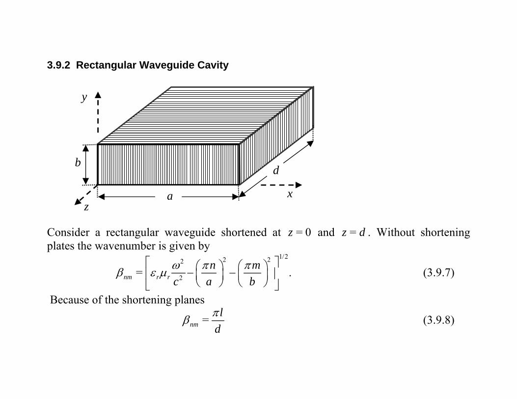
3.9.2 Rectangular Waveguide Cavity
x
y
za
db
Consider a rectangular waveguide shortened at = 0z and =z d . Without shortening plates the wavenumber is given by
1/22 22
2= .nm r rn m
c a bω π πβ ε μ
⎡ ⎤⎛ ⎞ ⎛ ⎞− −⎢ ⎥⎜ ⎟ ⎜ ⎟⎝ ⎠ ⎝ ⎠⎣ ⎦
(3.9.7)
Because of the shortening planes
=nml
dπβ (3.9.8)
thus the resonance frequencies are given by
1/22 2 2
, ,1= .
2n m lr r
c n m lfa b dπ π π
π ε μ
⎡ ⎤⎛ ⎞ ⎛ ⎞ ⎛ ⎞+ +⎢ ⎥⎜ ⎟ ⎜ ⎟ ⎜ ⎟⎝ ⎠ ⎝ ⎠ ⎝ ⎠⎣ ⎦
(3.9.9)
We shall examine next electromagnetic field characteristics in a cavity. In particular we shall calculate the quality factor of a 101TE . Choosing > >d a b , this is the lowest mode. It has the following field (non-zero) components
0
cos
sin
sin
z
x
y r r
xj z j zH Ae Bea
j a xj z j zH Ae Bea
j a xj z j zE Ae Bec a
πβ β
β πβ βπω πβ βε μ ηπ
⎛ ⎞−⎡ ⎤= + ⎜ ⎟⎢ ⎥⎣ ⎦ ⎝ ⎠⎛ ⎞−⎡ ⎤= − ⎜ ⎟⎢ ⎥⎣ ⎦ ⎝ ⎠
⎛ ⎞−⎡ ⎤= − + ⎜ ⎟⎢ ⎥⎣ ⎦ ⎝ ⎠
(3.9.10)
Bearing in mind that yE vanishes at = 0z we obtain = 0A B+ and applying the
same condition at =z d we get = 0 si2 n( ) = 0j d j dAe Be jA dβ β β− − ⇒ − therefore for a non trivial solution β has to satisfy =d lβ π which is just (3.9.8).

Consequently, the mode 101TE is described by
1/22 2
2
( , ; ) 2 cos sin
( , ; ) 2 sin cos
( , ; ) 2 sin sin
z
x
y
x zH x z jAa d
a x zH x z jAd a d
a a x zE x z Ad d a d
π πω
π πω
π π π πω ηπ
⎛ ⎞ ⎛ ⎞= − ⎜ ⎟ ⎜ ⎟⎝ ⎠ ⎝ ⎠⎛ ⎞ ⎛ ⎞= ⎜ ⎟ ⎜ ⎟⎝ ⎠ ⎝ ⎠
⎡ ⎤⎛ ⎞ ⎛ ⎞ ⎛ ⎞= − +⎢ ⎥⎜ ⎟ ⎜ ⎟ ⎜ ⎟⎝ ⎠ ⎝ ⎠ ⎝ ⎠⎢ ⎥⎣ ⎦
(3.9.11)
The electric and the magnetic energy stored in the system
2 2 2
2 2 22 2 20 0 0
1 1= | | | 2 | =4 4 2 2
a b d
E o y o Ma a dW dx dy dz E A b W
a dπ πε ε η
π⎡ ⎤
= +⎢ ⎥⎣ ⎦
∫ ∫ ∫
Clearly at resonance the electric energy equals the magnetic energy stored in the system therefore the total average energy stored in the cavity is
2
22
1= 2 = ( ) 1 | | .2T E o
aW W bad Ad
μ⎡ ⎤+⎢ ⎥
⎣ ⎦ (3.9.12)
Next we shall calculate the loss. The surface current is given by =sJ n H× therefore the dissipated power is given by
( )
2 222
loss
2 3 3 3 3 2
| |1 1 1 1= = = = | |2 2 2 2
=| | 2 2 /
s x sx
s
J H RJP da da da da H
A R a b d b ad da d
δ δσ δ σ δσ
⎛ ⎞⎜ ⎟⎝ ⎠
+ + +
∫ ∫ ∫ ∫ (3.9.13)
Consequently, the quality factor
( ) ( )
3/22 2 3
2 3 3 3 3
/ / ( )2= = = .2 (2 2 )
T E
loss loss s
a d adW WQP P R a b d b a d d a
π πω ω ηπ
⎡ ⎤+⎣ ⎦+ + +
(3.9.14)
As an example consider the following parameters [ ] [ ] [ ] [ ]
[ ]
7Cu
0
0.14 nsec5.8 10 Ohm/m , = = = 3 cm = 7.0 GHz , = 1/
0 0.5.02 8 ms2 , 12700, = 2 = / ec/ .s
a b d f T f
R Q Q Q f
σ
τ ω π
× →
Ω
∼
∼ ∼
In the case of dielectric losses
ef
2loss,
loss f,
1 2= | | = 1 1=2
1=d
Ed dV
d
WP dV E QP Q Q Qω εωε
ε′
′′ ⇒ ⇒′
+′∫ (3.9.15)
since the total power loss is the sum of the two mechanisms. Exercise 3.18: Check whether (3.9.13) is correct. In particular check if zH does not contribute to the relevant surface current. Calculate the impedance in (3.9.6).

3.9.3 Cylindrical Resonator In this subsection we briefly repeat the
previous exercise in cylindrical geometry. Consider a cylindrical waveguide of radius R . with two shorting planes at = 0z and =z d . We shall examine in this case the 11TE mode
1 11= coszr j z j zH J p Ae BeR
β βφ⎛ ⎞ −⎡ ⎤′ +⎜ ⎟ ⎢ ⎥⎣ ⎦⎝ ⎠ (3.9.16)
wherein 11 = 1.841p′ . Determine all the other field components!! As in the previous subsection
( = 0, ) = 0
2 sin( ) = = / .( = 0, ) 0
rE z djA d d d
E z dφ
β β π β π⎫⇒ − ⇒ ⇒⎬= ⎭
(3.9.17)
thus
1/22 2
11= .pc d Rω π⎡ ⎤′⎛ ⎞ ⎛ ⎞+⎢ ⎥⎜ ⎟ ⎜ ⎟
⎝ ⎠ ⎝ ⎠⎣ ⎦ (3.9.18)
2R
d

Exercise 3.19: Prove that the quality factor for a TE mode is given by
( )
( )
( )
3/22 22
222
11=
2 1 2
nmnmTE
nml
snm
nm
n lp Rp d
QR l R nl Rp Rc d d d p d
π
ω π πδ
⎡ ⎤ ⎡ ⎤⎛ ⎞ ⎛ ⎞′⎢ ⎥− +⎢ ⎥⎜ ⎟ ⎜ ⎟′ ⎝ ⎠⎢ ⎥ ⎢ ⎥⎝ ⎠ ⎣ ⎦⎣ ⎦⎛ ⎞⎛ ⎞ ⎛ ⎞′ + + − ⎜ ⎟⎜ ⎟ ⎜ ⎟ ′⎝ ⎠ ⎝ ⎠⎝ ⎠
(3.9.19)
For a TM mode the quality factor is given by
( )
1/222
0
> 01 1 2=
= 01
nm
TMnml
snm
lp Rd
lRQ d
pc lRd
π
ω δ
⎧⎡ ⎤⎛ ⎞⎪ +⎢ ⎥⎜ ⎟⎪ ⎝ ⎠⎢ ⎥⎣ ⎦⎪⎪ +⎨⎪⎪⎪
+⎪⎩
(3.9.20)
Exercise 3.20: Retrieve the result in (3.9.19)--(3.9.20). Compare to a rectangular cavity of the same volume or same surface.

3.9.4 Open Resonator – Circular Geometry
In many cases the cavity relies on evanescent waves that decay in one direction and they do not carry any power in that direction. One example is illustrated below: A cylindrical waveguide of radius R with a short-circuiting plane at z=0, a dielectric ( )rε of thickness d .
Exercise 3.21: Determine the resonant frequency and the quality factor for a TMnm mode. Repeat the exercise for TEnm mode. Consider both metallic and dielectric loss.
2R
d
rε

3.9.5 Exciting a Cavity
There are two main methods to excite cavities: with coaxial line (electric or magnetic coupling) or with a waveguide through an aperture.
In what follows, we shall consider a simple example
of excitation of a cavity by a waveguide through a small (circular) aperture of radius 0r as illustrated in lower frame. Ignoring loss processes the input impedance is given by the parallel impedance of the aperture
( )( tan )= .tan( )
Lin
L
j X j dZj X j d
ββ+
(3.9.21)
To include propagation loss (still assuming ideal aperture) the input impedance is
tanh( )= .tanh( )
Lin
L
j X d j dZj X d j d
α βα β
++ +
(3.9.22)
Cavity
Waveguide Aperture
Coaxialline
(a)
Coaxialline
(b)
(c)
0=z
1=cZ LXj
y
z
b
dz =d d
02r
( )a ( )b

In case of a TE10 the normalized impedance of the aperture is 2
00
8=3
LrX r
abπ β
π⎛ ⎞⎜ ⎟⎝ ⎠
revealing that this is proportional to the areas ratio. For low loss
( ) tan( )tan tanh( )
Lin
L
j X j LZj X j d
ββ α+ +
(3.9.23)
and the condition for resonance ( ) tan = 0LXω β≡ +D (3.9.24)
implies that at resonance ( 0ω ω= )
2
0( = ) .Lin
XZd
ω ωα
(3.9.25)
In the vicinity of the resonance
2
in 0in
0 0= =0 0
( = )( )( ) 1 ( )
L ZXZjd jdω ω ω ω
ω ωωα ω ω ω ω
ω α ω∂ ∂⎛ ⎞+ − + −⎜ ⎟∂ ∂⎝ ⎠D D
(3.9.26)
Since for an RLC circuit the impedance in the vicinity of the resonance is [ ] 1
in in 0 0( ) ( = ) 1 ( ) /Z Z jω ω ω ω ω ω −+ − Δ we conclude by analogy that the bandwidth is ( )0/ =dω α ω ω′Δ = D implying that the quality factor ( )0 0 0/ = /Q dω ω ω ω ω α′= Δ = D .

Comment: It is interesting to note that ( )0=ω ω′D depends on the group velocity since =LX U dβ
( )
( )0
0 2= 0
2 2
1= = [ tan( )] =cos
= 1 tan = [ 1 ( ) ]gr gr
U d d d Ud
d dU d U U dV V
ω ω
ω ω
βω ω β βω ω β
β β=
⎡ ⎤∂ ∂′ + +⎢ ⎥∂ ∂ ⎣ ⎦
⎡ ⎤+ + + +⎣ ⎦
D
(3.9.27)
where 2
0 08=3
r rUab dπ
π⎛ ⎞⎜ ⎟⎝ ⎠
implying that the quality factor is inversely proportional to the
group velocity in the waveguide consisting the cavity ( )0= 1/ grQ Vω ω′∝ ∝D .

3.10 Wedge in a Waveguide 3.10.1 Metallic Wedge The goal of this section is to analyze a wave guide of a circular cross-section but which lacks a slice as illustrated below
In order to keep the problem relatively simple, we shall limit the discussion to the evaluation of the cut-off frequency. For this purpose we recall that in Section 2.1 we
x
y
α
2R

found that
z2 2
z2 2
2 2 2
= 1
= 1
z z z
z z z
jk jE E Hk kjk jH H Ek k
k k
ωμ
ωε
ω εμ
⊥ ⊥ ⊥⊥ ⊥
⊥ ⊥ ⊥⊥ ⊥
⊥
− ∇ + ×∇
− ∇ − ×∇
= −
(3.10.1)
And both longitudinal components satisfy the wave equation. Limitint the analysis to the cut-off frequencies 0zk = these equations simplify
1 11= 1
1
1 11= 1
1
r z
z z
z
r z
z z
z
E Hj r
E Hj E H
j r
H Ej r
H Ej H E
j r
φ
φ
ωε φωε
ωε
ωμ φωμ
ωμ
⊥ ⊥
⊥ ⊥
∂⎧ =⎪ ∂⎪− ×∇ ⇒ ⎨ ∂⎪ = −⎪ ∂⎩
− ∂⎧ =⎪ ∂⎪+ ×∇ ⇒ ⎨ ∂⎪ =⎪ ∂⎩
(3.10.2)
and the wave equation simplifies
α
2R

22
2 2
1 1 0z
z
Er
Hr r r rω με
φ⎛ ⎞⎛ ⎞∂ ∂ ∂
+ + =⎜ ⎟⎜ ⎟∂ ∂ ∂ ⎝ ⎠⎝ ⎠ (3.10.3)
Obviously, the solution of this set of equations describe a resonator whereby the field does not vary in the z-direction. For the TM modes the solution is of the form
( ) ( ) ( ) ( ), cos sinzE r J qr A Bνφ νφ νφ⎡ ⎤∝ +⎣ ⎦ (3.10.4) subject to the boundary conditions
( )( )( )
, / 2 2 / 2 0
, / 2 0
, 2 / 2 0
z
z
z
E r R
E r
E r
α φ π α
φ α
φ π α
= < < − =
= =
= − =
(3.10.5)
The first condition implies that ( ) 0J qRν = (3.10.6)
wherein q is yet to be determined and from the other two conditions we will specify :ν
( ) ( ) ( )( ) ( ) ( )
, / 2 0 cos / 2 sin / 2 0
, 2 / 2 0 cos 2 / 2 sin 2 / 2 0z
z
E r A B
E r A B
φ α να να
φ π α ν π α ν π α
= = ⇒ + =
⎡ ⎤ ⎡ ⎤= − = ⇒ − + − =⎣ ⎦ ⎣ ⎦(3.10.7)
or explicitly
α
2R
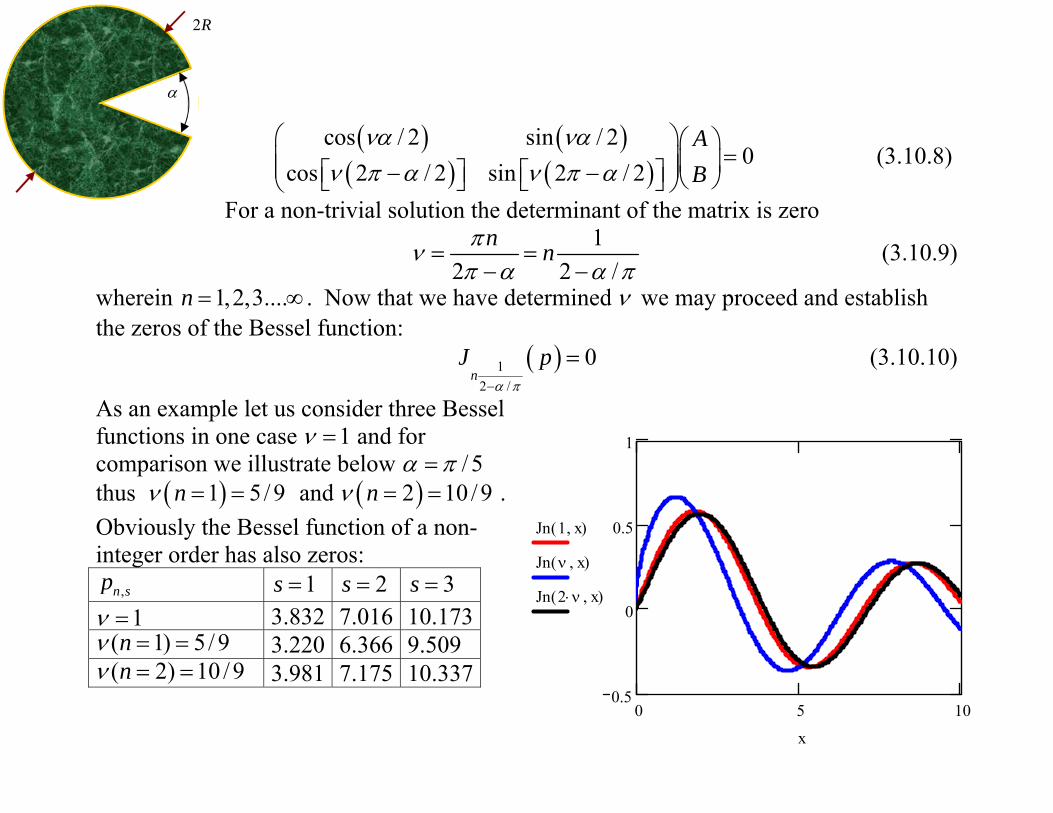
( ) ( )( ) ( )
cos / 2 sin / 20
cos 2 / 2 sin 2 / 2AB
να ναν π α ν π α
⎛ ⎞⎛ ⎞=⎜ ⎟⎜ ⎟⎜ ⎟⎡ ⎤ ⎡ ⎤− − ⎝ ⎠⎣ ⎦ ⎣ ⎦⎝ ⎠
(3.10.8)
For a non-trivial solution the determinant of the matrix is zero
12 2 /
n nπνπ α α π
= =− −
(3.10.9)
wherein 1,2,3....n = ∞ . Now that we have determined ν we may proceed and establish the zeros of the Bessel function:
( )12 /
0n
J pα π−
= (3.10.10)
As an example let us consider three Bessel functions in one case 1ν = and for comparison we illustrate below /5α π= thus ( )1 5/ 9nν = = and ( )2 10 /9nν = = . Obviously the Bessel function of a non-integer order has also zeros:
,n sp 1s = 2s = 3s = 1ν = 3.832 7.016 10.173
( 1) 5/9nν = = 3.220 6.366 9.509 ( 2) 10 /9nν = = 3.981 7.175 10.337
0 5 100.5
0
0.5
1
Jn 1 x,( )
Jn ν x,( )
Jn 2 ν⋅ x,( )
x
α
2R

Explicitly
( )
( )
, 1 ,, 1 2 /
, 12 /
/ 2, sin2
: 0
z n s n snn s
n s n
rE r U J p nR
p J pα π
α π
φ αφ ππ α
∞
= −
−
−⎛ ⎞ ⎛ ⎞= ⎜ ⎟ ⎜ ⎟−⎝ ⎠ ⎝ ⎠
=
∑
(3.10.11) and the cut-off frequencies are determined by
co ,n sc pR
ω = (3.10.12)
The top frame in the right reveals the contours of constant zE for
1and 1s n= = . The central frame illustrates the case 1and 2s n= = whereas the lower frame corresponds to 2and 1s n= = .
Ez2
Ez
Ez3
α
2R

A similar approach may be followed for the TE modes
( ) ( ) ( ) ( ), cos sinzH r J qr A Bνφ νφ νφ⎡ ⎤∝ +⎣ ⎦ (3.10.13) subject to the boundary conditions
( )( )( )
, / 2 2 / 2 0
, / 2 0
, 2 / 2 0r
r
E r R
E r
E r
φ α φ π α
φ α
φ π α
= < < − =
= =
= − =
(3.10.14)
The first condition [Eq. (3.10.2)] implies that
( ) 0r R
d J qrdr ν
=
⎡ ⎤ =⎢ ⎥⎣ ⎦ (3.10.15)
wherein q is yet to be determined and from the other two conditions we specify :ν
( ) ( ) ( )( ) ( ) ( )
, / 2 0 sin / 2 cos / 2 0
, 2 / 2 0 sin 2 / 2 cos 2 / 2 0r
r
E r A B
E r A B
φ α να να
φ π α ν π α ν π α
= = ⇒ − + =
⎡ ⎤ ⎡ ⎤= − = ⇒ − − + − =⎣ ⎦ ⎣ ⎦(3.10.16)
or explicitly
( ) ( )( ) ( )
sin / 2 cos / 20
sin 2 / 2 cos 2 / 2AB
να ναν π α ν π α
⎛ ⎞− ⎛ ⎞=⎜ ⎟⎜ ⎟⎜ ⎟⎡ ⎤ ⎡ ⎤− − − ⎝ ⎠⎣ ⎦ ⎣ ⎦⎝ ⎠
(3.10.17)
For a non-trivial solution the determinant of the matrix is zero

12 2 /
n nπνπ α α π
= =− −
(3.10.18)
wherein 1,2,3....n = ∞ . Now that we have determined ν we may proceed and establish the zeros of the Bessel function:
( )12 /
0n
J pα π−
′ = (3.10.19)
From here the approach is virtually identical
( )
( )
, 1 ,, 1 2 /
, 12 /
/ 2, cos2
: 0
z n s n snn s
n s n
rH r U J p nR
p J pα π
α π
φ αφ ππ α
∞
= −
−
−⎛ ⎞ ⎛ ⎞′= ⎜ ⎟ ⎜ ⎟−⎝ ⎠ ⎝ ⎠′ ′ =
∑ (3.10.20)
Exercise 3.22: Draw the contours of constant zH . Compare the field distribution of the TE and TM modes. For both modes compare the magnetic and electric energy per-unit length.

3.10.2 Dielectric Wedge The goal of this section is to analyze a waveguide of a circular cross-section but which has a material ( ),r rμ ε slice as illustrated below As in the metallic case we keep the problem relatively simple, and limit the discussion to the evaluation of the cut-off frequency. As a result, we can separate the analysis of the TE and TM modes. So let us start with the TM mode.
Vacuum Slice 2 2
2 2 2
0
0
1 1 0
1 1
1
z
r z
z
r Er r r r c
H Ej r
H Ej rφ
ωφ
ωμ φ
ωμ
⎛ ⎞∂ ∂ ∂+ + =⎜ ⎟∂ ∂ ∂⎝ ⎠
− ∂=
∂
∂=
∂
2 2
2 2 2
0
0
1 1 0
1 1
1
r r z
r zr
zr
r Er r r r c
H Ej r
H Ej rφ
ω μ εφ
ωμ μ φ
ωμ μ
⎛ ⎞∂ ∂ ∂+ + =⎜ ⎟∂ ∂ ∂⎝ ⎠
− ∂=
∂
∂=
∂A differential approach (separation of variables) is not applicable since the radial
x
y
2R
α
( ),r rμ ε
11
r
r
με
==

variation needs to be the same in both regions but if this is the case the function does not satisfy the wave equation. We must seek an integral approach. For determining the cut-off frequencies associated with the TM-like modes we need to solve
( )2 2 2
2 2 2 2
1 1z zr E f E
r r r r c cω ω φ
φ⎛ ⎞∂ ∂ ∂
+ + = −⎜ ⎟∂ ∂ ∂⎝ ⎠ (3.10.21)
wherein ( )f φ is a function which equals 1r rμ ε − in the region(s) with material and zero otherwise. A solution which satisfies the boundary conditions
( ) ( ), ,1
, expz n s n n sn s
rE r J p jnR
φ φ∞ ∞
=−∞ =
⎛ ⎞= ⎜ ⎟⎝ ⎠
∑ ∑E (3.10.22)
substituting in (3.10.21) we get
( ) ( ) ( ) ( )
( ) ( )
2 2 2,, ,
, , , , ',2 2 21
1 1, ' , ', ' ' ', ' , , , ' , ,
0 0
',
,
1 exp '2
n ss s sn s n n m m n n m
m
s s s sn n n n s n n s n n s s n n s n n s
n m
pF
R c c
dx xJ p x J p x dx xJ p x J p x
F d f j n m
σσ
σ
π
π
ω ωχ χ
χ χ δ
φ φ φπ
∞ ∞
=−∞ =
−
⎛ ⎞− + = −⎜ ⎟⎝ ⎠
≡ =
⎡ ⎤= − −⎣ ⎦
∑ ∑
∫ ∫
∫
E E
(3.10.23)

Rewriting 2
, , 2, , , , , , , ,
1
s s sm m n n m n m s n s n n n s
mR F p
cσ
σ σσ
ω χ δ δ χ∞ ∞
=−∞ =
⎛ ⎞ ⎡ ⎤+ =⎜ ⎟ ⎣ ⎦⎝ ⎠∑ ∑E E (3.10.24)
and defining the matrices
,,
, , ,, , , , 2, ,
sm n
n m n m sn s m s sn n n s
C Fp
σ
σσ
χδ δ
χ⎡ ⎤= +⎣ ⎦ (3.10.25)
thus defining /R cω ω= .
2, , , , , , , ,
, ,n s m m n s m m
m mC Iσ σ σ σ
σ σ
ω−=∑ ∑E E (3.10.26)
implying that the (square of the ) cut-off frequencies are the inverse of the eigen-values of the matrix C
2 0ω−− =C I . (3.10.27)
Exercise 3.23: Calculate the first cut-off frequency of a waveguide with dielectric slice identical with the metallic slice. Compare the two results. Examine the convergence of the solution. Exercise 3.24: Repeat Exercise 3.23 for the TE mode including the formulation.

3.11 Appendix 3.11.1 Solution to Exercise 3.8
Analyze (numerically) the dependence of the normalized reactance on three parameters; the angular frequency ( )ω , its location ( )d and its radius ( )R .
The normalized reactance of a cylindrical post located
in a rectangular waveguide as a function of f . The normalized reactance given by Eq. (3.4.20) is shown to increase with frequency, which implies an inductive behavior. [ = 2.5a cm, = 1b cm, = 1rε , = / 2 = 1.25d a mm,
= / 20R a , = 2,3, 200n ].
x a
b
d
y
2R
x a
b
d
y
2R[ ]GHzf
X
0.3
0.4
0.5
0.6
8 9 10
L

The normalized reactance of a cylindrical post
located in a rectangular waveguide as a function of d . The solid line and the dotted line correspond to
= 8f GHz and = 10f GHz, respectively. A minima in the normallized reactance is observed at the middle of the rectangular waveguide, whereas close to the edges the normalized reactance increases. [ = 2.5a cm, = 1b cm, = 1rε , = / 20R a ,
= 2,3, 200n ].
0
2
4
6
[ ]GHz10
[ ]GHz8
[ ]mmd
5 10 15 20
XL
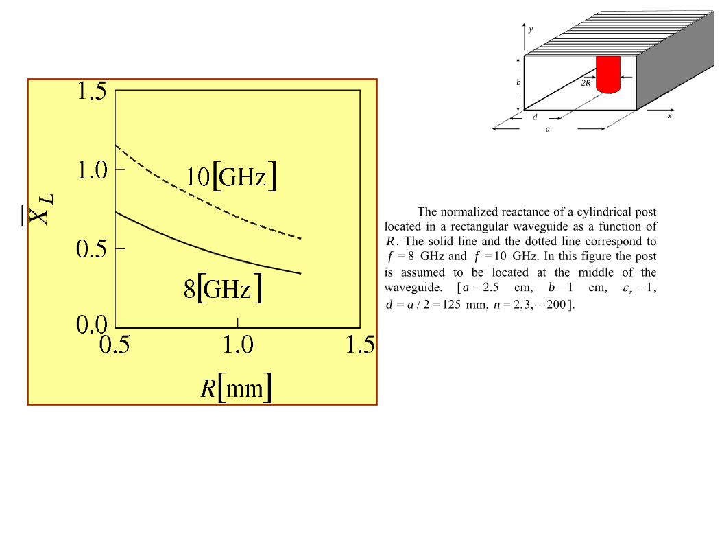
The normalized reactance of a cylindrical post
located in a rectangular waveguide as a function of R . The solid line and the dotted line correspond to
= 8f GHz and = 10f GHz. In this figure the post is assumed to be located at the middle of the waveguide. [ = 2.5a cm, = 1b cm, = 1rε ,
= / 2 = 125d a mm, = 2,3, 200n ].
x a
b
d
y
2R

The normalized reactance of a cylindrical post located in a rectangular waveguide as a function of R . The solid line and the dotted line correspond to = 8f GHz and = 10f GHz, In this figure the post is assumed to be located close to one of the edges of the waveguide. [ = 2.5a cm, = 1b cm, = 1rε , = 5d mm, = 2,3, 200n ].
x a
b
d
y
2R
[ ]GHz10
[ ]mmR
0.5 1.0 1.50.0
0.5
1.0
1.5
[ ]GHz8
XL

Chapter 4: Matrix Formulations
4.1 Impedance Matrix
Consider an N port systems that is characterized at a given frequency by set of complex
numbers ijZ ∼ i.e. 22N parameters
11 1
1
1 1
2=
N
NN NNN
Z Z
Z Z
V I
V
V I
(4.1.1)
or, explicitly,
=0
= .iij
jk j
VZ
II ≠
(4.1.2)
1V
2V
NV
1I
2I
NI

In a similar way we can define the admittance matrix
1 111 1
21 2
1
2 2
= .
N
N
N NN NN
Y Y
Y Y
Y Y
I V
I V
I V
(4.1.3)
Example: For the sake of simplicity, let us determine the Z matrix of a section of
transmission line.
This two port system is characterized by
1 11 12 1
2 21 22 2
=V Z Z I
V Z Z I
(4.1.4)
and for example the first term is
111
1 =02
=V
ZI I
(4.1.5)
wherein 2 = ( = )I I z− . Without loss of
generality, the voltage and current wave are
given by
1I 2I
1V 2V
0=Z =Z
0Z

( ) =j z j z
V z V e V eβ β
+ −− +
1
( ) =o
j z j zI z V e V e
Z
β β+ −− −
(4.1.6)
respectively. At the ``input'', i.e. at = 0z
1 1
1= = ( ).
o
V V V I V VZ
+ − + −+ − (4.1.7)
Based on (4.1.5) we explicitly have
11 =
( )=0o
V VZ Z
V V I
+ −
+ −
+−
(4.1.8)
wherein the condition ( ) = 0I implies
1 2
( ) = = 0 =o
j j jI V e V e V V e
Z
β β β+ − − +− − −
(4.1.9)
hence
11
21 cos( )
= = = ctan( )2 sin1
−+−
−−
o o o
je
Z Z Z jZj je
β βββ β
(4.1.10)
11 = ctan( ).− oZ jZ β (4.1.11)

In a similar way we may establish the other parameters of the matrix. For example,
112 0
2 =01
= =
( )
V V VZ Z
j jI V e V eIβ β+ −
+ −
+− − −
(4.1.12)
and since [ ]1
1= =
o
I V V V VZ
+ − + −− we get
012 0
2= =
sin( )
jZZ Z
j je e
β β β−
− − − (4.1.13)
In a similar way 21 12=Z Z and 22 11=Z Z implying
ctan( )sin
= .
ctan( )sin
− −
− −
o
o
o
o
jZjZ
ZjZ
jZ
θθ
θθ
(4.1.14)

4.2 Scattering Matrix
In many cases it is more convenient to measure the
amplitudes of the reflected and transmitted waves
1 111 1
2 2
1
=
N
N NNN N
v vS S
v v
S Sv v
− +
− +
− +
(4.2.1)
1 11 1
o o
v vv v
Z Z
+ −+ −≡ ≡ (4.2.2)
the reason for this normalization becomes evident since
*
2*1 ( ) 1
= = = ( ) .2 2 2o o
V VP V v v
Z Z
+ ++ ++ (4.2.3)
+1V
−1V
+2V
−2V
+NV
−NV

The S matrix elements are defined by
=0
= .i
ij
jk j
vS
v v
−
++≠
(4.2.4)
In order to achieve = 0kv+
the port is loaded with a
matched impedance, namely
the diagonal term iiS represents the reflection
coefficient at the i th port when all the other ports are
matched.
Describing linear systems, both S and Z matrices
are interrelated. Firstly it is convenient to define
=ij
ij
o
ZZ
Z, =
o
vv
Z and = oI I Z consequently
=v v v+ −+ and =I v v
+ −− .
Using now the definition of the Z matrix
= =v v v Z v v+ − + − + −
(4.2.5)
0Z 0Z
0=+kv
−kv

[ ] = [ ]I Z v I Z v+ −
− − + (4.2.6)
thus since =v Sv− +
1= ( ) ( ).S Z I Z I−+ − (4.2.7)
Properties of the S matrix:
Property 1: If the system is reciprocal S is symmetrical
= or = .t
ij jiS S S S (4.2.8)
This is true provided that at all ports the power is given by 21
| |2
nv i.e. characterization
impedance at all ports is the same. In order to prove this statement we recall that based on
Lorentz reciprocity theorem (in absence of sources)
1 2 2 1 = 0 =i j j i
s i jE H E H nds E H da E H da × − × ⋅ ⇒ × × ∫ ∫ ∫
(4.2.9)
and since the electric field is associated with the voltage whereas the local magnetic
field is linked to the current 1 1 2 2,E V H I∼ ∼ thus
= .i j j jv I v I (4.2.10)

Bearing in mind that =i j ij jI Y vΣ and =j i ji iI Y vΣ we conclude that
= = =i j i jij ji ij ji ij jiv v Y v v Y Y Y Z Z⇒ ⇒ (4.2.11)
Namely both the admitance and impedance matrices are symmetric aobviously since 1= ( ) ( 1)S Z I Z
−+ − if Z is symmetrical so is S
= .ij jiS S (4.2.12)
Property 2. For a lossless system, S is unitary namely
1 * *
= ( ) ( ) = .T
S S S S I− +
(4.2.13)
For prooving this statement we bear in mind that power conservation implies
* * **
* * ***
0 0
0 0
T TT T
T T Tt t
v v v v v I v Sv Sv
v I v v S S v v I S S v
− + + + ++ + −
+ + + + + +
− = ⇒ − =
− = ⇒ − =
(4.2.14)
Example: Consider a two ports system with a load LZ at the output

1 111 12
21 222 2
=S Sv v
S Sv v
− +
− +
(4.2.15)
whereas the load
2
2
= = = .L oL L
L o
Z Z vS
Z Z vρ
+
−
−+
(4.2.16)
Combining the two entails
1 1 2 1 211 12 11 12= = Lv S v S v S v S S v− + + + −
+ +
2 1 2 2 121 22 22 21= (1 ) =L Lv S v S S v v S S S v− + − − +
+ → − (4.2.17)
Thus the reflection coefficient
1 12 2111
1 22
= = = .1
Lin in
L
v S S SS S
v S Sρ
−
+ +−
(4.2.18)
+1v
+2v
−2v
LZ
−1v

4.3 Transmission Matrix
1 2
1 2
=v vA B
I IC D
(4.3.1)
1 11 1 12 2
2 21 1 22 2
=
=
v Z I Z I
v Z I Z I
−
− (4.3.2)
Thus
2
11 11 22 12
1 112 12
1 122
12 12
=1
Z Z Z Z
v vZ Z
I IZ
Z Z
−
(4.3.3)
Det 1≡ABCD (4.3.4)
1v 2v
1I 2I

4.4 Wave-Amplitude Transmission Matrix
1 211 12
21 221 2
=T Tv v
T Tv v
− +
+ −
(4.4.1)
Relation to S matrix
11 22 11 2211 12 12 21 22
21 21 21 21
1= , = , = , =
S S S ST S T T T
S S S S− − (4.4.2)
In a reciprocal system S is symmetrical and 12 21=S S . Therefore
12
21
Det( ) = = 1S
TS
(4.4.3)
+1v
+2v
−2v
−1v

Example: Scattering and transmission matrices of a section of transmission line
11 121 1
21 222 2
=S Sv v
S Sv v
− +
− +
(4.4.4)
1 2 1 211 22 12 21
1 2 2 1=0 =0 =0 =02 1 1 2
= = 0, = = 0, = = , = =v v v vj j
S S S e S ev v v vv v v v
β β− − − −
+ + + ++ + + +
− −
(4.4.5)
00
= =
00
je j
eS T
jej
e
ββ
ββ
− −
− −
(4.4.6)
0Z
+1v
−2v
−1v
+2v

4.5 Loss Matrix
Based on the result in Eq.(4.2.14)
*= ( )TQ I S S− (4.5.1)
and since the dissipated power is
*
dis
1= ( )
2
+ + −
TT
P v I S S v (4.5.2)
the matrix defined above determines this dissipated power
dis
1=
2
+ +
T
P v Qv . (4.5.3)

4.6 Directional Coupler
• 4 ports, lossless and reciprocal
• At least one symmetry plane
• Each port is matched when all
the
other are loaded with oZ
• The power entering (1) splits
equally between (3) and (4).
No power reaches (2).
Performance parameters:
( )( )
1 4
4 2
Coupling : = 10log /
Directivity : = 10log /
C P P
D P P
S matrix:
12 21 34 43
11 22 33 44
13 31 23 32 14 41 24 42
Isolation condition : = = = = 0
Matching condition : = = = = 0
Symmetrical condition : = , = , = , =
S S S S
S S S S
S S S S S S S S
13 14
23 24
13 23
14 24
0 0
0 0
0 0
0 0
S S
S SS
S S
S S
=
1
2
3
4
input
insulated
direct
coupled

4.7 Coupling Concepts
We shall discuss several aspects of the coupling effect. Here we shall investigate
coupling in transmission line configuration.
4.7.1 Double Strip Line: Parameters of the Line
The basic configuration under consideration is illustrated above. Each one of the wires is
x=0
x=a
z=0
a/2
∆
(1) (2)
δ
x
z

charged thus the charge distribution in the system is assumed to be
1 1 2 2( , ) = , ( , ) =2 2 2 2
a ax z x z x z x zρ λδ δ ρ λ δ δ
∆ ∆ − − − +
For the electrostatic potential we may write the following expression
=1
( , ) = ( )sinn
n
nxx z z
a
πϕ
∞ Φ
∑
Which satifies the boundary conditions on the two plates. This potential satisfies the
Poisson equation i.e.,
2 2
2 2
22
2
1( , ) = ( , )
1 2( ) = ( , )sin
1 2= sin
2 2
o
n
o
o
x z x zx z
d n nxz dx x z
dz a a a
nz
a
νν
ν
ϕ ρε ε
π πϕ ρ
ε ε
πλ δ
ε ε
∂ ∂+ − ⇒ ∂ ∂
−
∆ − −
∫
∑
(4.7.1)
where = 1,2ν and 1 2= , =∆ ∆ ∆ −∆ .
1 2
=1
1( , ) = sin sinc exp exp
2 2 2 2n
nx n n nx z z z
a a a
π πϕ λ π λ π
∞ ∆ ∆ − + + − −
∑ (4.7.2)

For a strip of width δ we have
2 2
1
2 2
=12 2
2
2 2
1( )exp
1( , ) = sin sinc
2 21
( )exp
n
nd z
anx
x z na
nd z
a
δ
δ
δ
δ
πξλ ξ ξ
δπ π
ϕ
πξλ ξ ξ
δ
∆− +
∆∞ − −
∆+
∆−
− −
+ − −
∫
∑
∫
(4.7.3)
Assuming that 1( )λ ξ and 2 ( )λ ξ are uniform
=1
2 2 2 2
1 2
2 2 2 2
1( , ) = sin sinc
2 2
exp
n
nxx z n
a
nd d z
a
δ δ
δ δ
π πϕ
λ λ πξ ξ ξ
δ δ
∞
∆ ∆− + +
∆ ∆− − −
× + − −
∑
∫ ∫(4.7.4)
Moreover, the potential is uniform on the strip

2 2
1
2 2
2 2 2 2
1
=1
2 2 2 2
2 2 2 2
2
=1
2 2 2 2
1( , )
2
1= sin sinc exp
2 2 2
1sin sinc exp
2 2 2
n
n
aV dz x z
n nn dz d z
a
n nn dz d z
a
δ
δ
δ δ
δ δ
δ δ
δ δ
ϕδ
λ π π πξ ξ
δ δ
λ π π πξ ξ
δ δ
∆− +
∆− −
∆ ∆− + − +
∞
∆ ∆− − − −
∆ ∆− + +
∞
∆ ∆− − −
= =
− −
+ − −
∫
∑ ∫ ∫
∑ ∫ ∫
(4.7.5)
The integrals may be evaluated analytically therefore
2
11
=1
2
2
12
=1
1= sinc 1 exp sinhc
2 2 2 2
1= sinc sinhc
2 2exp
2 2
n
n
n
a
a n n nU
a a
a n n nU
a a
π π δ π δδ
π π δ π δδ
π
∞
∞
− −
− ∆
∑
∑ (4.7.6)
Similar considerations can be applied to the second strip hence 2 21 1 22 2=V U Uλ λ+
and detailed calculation shows that 21 12 22 11= and =U U U U . Note that the off

diagonal term is proportional to
)exp ( nna
π∆ −
∑ (4.7.7)
which indicates that the coupling drops rapidly. Furthermore, 11U are ∆ independent!
If the strips have different geometries 11 22=U U/ but still 12 21=U U . In a matrix form:
1 11 12 1 1 11 12 1
2 21 22 2 2 12 22 2
= =
V U U C C V
V U U C C V
λ λ
λ λ
⇒
(4.7.8)
A similar approach can be applied for evaluation of the inductance
1 11 12 1
2 12 22 2
=
L L I
L L I
Φ Φ
(4.7.9)
Exercise 4.1: Analyze the coupling term.
Exercise 4.2: Calculate the inductance matrix and analyze the coupling term.
Exercise 4.3: Analyze the case when the two strips are not equally wide.
Exercise 4.4: Analyze the case when the two strips are not equally wide and are not in
the same plane.

4.7.2 Equations of the System
The transmission line equations in this case read
1
11 12 1
2 12 22 2
1
11 12 1
2 12 22 2
= =
= =
dV
L L Idzd
V j LI jdz
dV L L I
dz
dI
C C Vdzd
I j CV jdz
dI C C V
dz
ω ω
ω ω
− −
− −
(4.7.10)
It is convenient in this case to investigate the waves which propagate in this system
2
2
2= = ( ) =
d dIV j L j L j CV LCV
dz dzω ω ω ω− − − − (4.7.11)
Let us define the wavenumber matrix

2 2
11 12
2 2
12 22
2 2=
K K
L
K
K
K
Cω
≡
(4.7.12)
Assume a solution of the form j z
eβ−
2 2 2
11 12 1
22
2 2 2
12 22 2
0
( ) = 0 = 0
0
K K V
I K V
K K V
ββ
β
− − + ⇒ +
−
(4.7.13)
Explicitly this reads
2 2 2
11 12 1
2 2 2 2 4
11 22 12
2 2 2
12 22 2
= 0 ( )( ) = 0
K K V
K K K
K K V
ββ β
β
− ⇒ − − −
−
(4.7.14)
Let us assume for simplicity sake that the two lines are identical i.e. 11 22=K K hence
2 2 2
1
2 2 2 4
11 1 112 2( ) = =0K K K Kββ ± ±− − (4.7.15)
The eigen-vectors corresponding to 2β+ may be derived from one of the two equations

eg., 2 2 2
11 1 12 2( ) = 0K V K Vβ+− + threfore choosing 1 = 1V we get 2 2
112 2
12
= = 1K
VK
β+−− implying
that the normalized egen-vector is
1 / 2
=
1/ 2
V +
(4.7.16)
And in a similar way, the normalized eigen-vector corresponding to 2β− is
1/ 2
=
1/ 2
V −
−
(4.7.17)
The general solution has the form
( ) =z z z zj j j j
V z V Ae Be V Ce Deβ β β β+ + − −
+ −− + − + + + +
(4.7.18)

4.7.3 Simple Coupling Process
In this subsection we ignore reflections. The schematics of the system under
consideration is illustrated in the right. Consider a solution of the form
( ) =z zj j
V z V Ae V Beβ β+ −
+ −− −
+ (4.7.19)
At = 0z only the mode in the first line exists. The question is how the power varies with
the length L .
( ) ( )
( ) ( )
1/ 2 1/ 2
( ) =
1/ 2 1/ 2
1/ 2 1/ 2
=
1/ 2 1/ 2
z z
z z
z z
j jV z Ae Be
j jAe Be
j jAe Be
β β
β β
β β
+ −
+ −
+ −
− −
+ −
− − +
− − −
(4.7.20)
In the absence of coupling 11= = Kβ β+ −
1
2 L

11 11
1 0
( ) =
0 1
z zjK jKV z C e D e
− − +
(4.7.21)
Now since 0( = 0) =V z V for line 1 and ( = 0) = 0V z for line 2 we get 0=C V and = 0D
implying that the voltage on line 2 is always zero.
Let us reinstate the coupling process: the voltage along the transmission lines is
given by
0
0
/ 2 / 2
( = 0) = = = =2
0 / 2 / 2
V A BV
V z A B
A B
+ ⇒
−
(4.7.22)
hence
( ) ( )
( ) ( )
1cos
2
1exp
2
( ) =
1sinx
2
=2
1e p
2
o
o
o
V j zj z j ze e
VV z
j z j ze e V j zz j
zβ ββ ββ β
β ββ β β β
+ −+ −
+
−
−−+ −
+
+
− +− − + − − − − +
−
−
In order to illustrate the coupling process, we examine the voltage on each one of the
1
2 L

lines
( ) ( )1
1 1= exp cos( ) cos
2 2o o
V V j z z V zβ β β β+ − + − − + −
(4.7.23)
( ) ( )2
1 1= exp sin( ) sin
2 2o o
V jV j z z V zβ β β β+ − + − − + −
(4.7.24)
Schematically these voltages are illustrated in the figure in the right. If we terminate
the ``coupler'' at a length L such that
( )1=
2 2L
πβ β+ −− (4.7.25)
the voltage is maximum on line 2 and zero on line
1. Recall 2 2
11 12= K Kβ± ± . For simplicity we
shall assume 2 2
11 12K K hence
2
1211
11
1=
2
KK
Kβ± ± (4.7.26)
and
1
2 L

( )2 2 2
12 12
11
2
1211 11
2
1
1
11 1 11
1 1 1 1 1=
2 2 2 2
=
2
=2
KL
K K KL
K
K K L LK K K
β β
π π
+ −
− + − −
⇒
(4.7.27)
This clearly indicates that the coupling is directly related to the off diagonal term in the
matrix 2
K .
Exercise 4.5: Analyze L as a function of the geometry (separation ∆ , width δ and planes
separation a ) in the previous section. Make sure that the result is independent of the
number of harmonics.
1
2 L

Chapter 5: Nonlinear Components
5.1 Transmission Line with Resistive Nonlinear Load
Consider a transmission line with a non-linear load
0 0( ) = tanh( / ).L LV t V I I (5.1.1)
The voltage-wave has two components, +V propagating in the forward direction and −V
representing the reflected wave
( , ) =z z
V z t V t V tv v
+ − − + +
(5.1.2)
wherein v is the phase-velocity.
Load 0
Z
0z =

In a similar way the current 2
0
1= ( ).
∞
− −−∞∫W dt V tZ
0
1( , ) = .+ −
− − +
z zI z t V t V t
Z v v (5.1.3)
At the location of the load
0
( ) ( = 0, ) = ( ) ( )
1( ) ( = 0, ) = [ ( ) ( )]
L
L
V t V z t V t V t
I t I z t V t V tZ
+ −
+ −
= +
= − (5.1.4)
thus after substituting in the constitutive relation
0
0 0
1( ) ( ) = tanh [ ( ) ( )] .+ − + −
+ −
V t V t V V t V t
Z I (5.1.5)
It is convenient to define
0
0 0 0 0
= and =±± L
VVV Z
Z I Z I (5.1.6)
hence
= tanh( ).+ − + −+ −LV V Z V V (5.1.7)
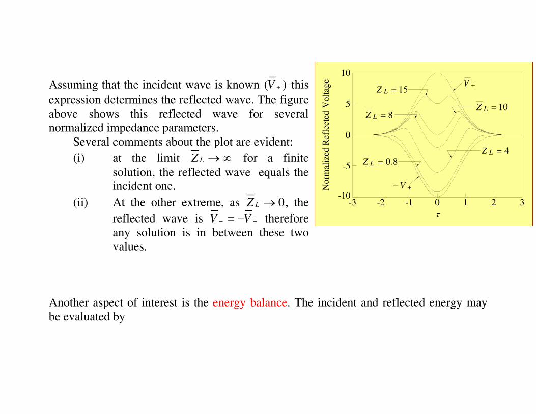
Assuming that the incident wave is known ( )+V this
expression determines the reflected wave. The figure
above shows this reflected wave for several
normalized impedance parameters.
Several comments about the plot are evident:
(i) at the limit →∞LZ for a finite
solution, the reflected wave equals the
incident one.
(ii) At the other extreme, as 0→LZ , the
reflected wave is =− +−V V therefore
any solution is in between these two
values.
Another aspect of interest is the energy balance. The incident and reflected energy may
be evaluated by
-3 -2 -1 0 1 2 3-10
-5
0
5
10
15=LZ
8=LZ
8.0=LZ
10=LZ
4=LZ
+−V
+V
τ
No
rmal
ized
Ref
lect
ed V
olt
age

2 2
0 0
1 1= ( ), = ( ).W dt V t W dt V t
Z Z
∞ ∞
+ + − −−∞ −∞∫ ∫ (5.1.8)
In a linear system the ratio of the two is
2
1=
1
−
+
−≡
+
L
WL
W Z
W Zρ (5.1.9)
wherein 0= /L LZ Z Z . The figure in the right illutrates Wρ
when the maximum value of the incident (Gaussian) wave
is (max )
= 2,5,10+V . This figure clearly reveals that there is
full reflection when LZ is zero or tends to infinity. Zero
reflection occurs when
(m
(maxax)
(max)0
0 0 0
)
0
0
= = .=L
V VZ V
Z I Z IV V+
++ ⇒ ⇒
0 5 10 15 200
0.2
0.4
0.6
0.8
1.0
LZ
Ra
tio
Energ
y
loadLinear
2max =V
5max =V
10max =V

Chapter 6: Periodic Structures
In a variety of applications it is necessary to control the phase velocity of the wave
or the propagation time. Periodic metallic or dielectric structures play an important role in
implementation of these devices. The periodic geometry can be conceived as a set of
obstacles delaying the propagation of the wave due to the multi-reflection process and, as
will be shown during our discussion on Floquet's theorem, an infinite spectrum of spatial
harmonics develops. A few of which cases these harmonics may propagate with a phase
velocity larger or equal to c but the absolute majority have a smaller phase velocity.
In the first section we present the basic theorem of periodic structures namely,
Floquet's theorem. This is followed by an investigation of closed periodic structures in
Section 6.2 and open structures in the third. Smith-Purcell effect is considered as a
particular case of a Green's function calculation for an open structure and a simple
scattering problem is also considered. The chapter concludes by presenting a simple
transient solution in a periodic structure.

6.1 The Floquet Theorem
A periodic function, ( )f z , is a function whose value at a given point z is equal to
its value at a point +z L i.e.,
( ) = ( ),+f z f z L (6.1.1)
where L is the periodicity of the function. Any periodic function can be represented as a
series of trigonometric functions exp( 2 / )− j nz Lπ and since this is an orthogonal and
complete set of functions, it implies
=
2 /( ) = .
∞
−∞
−∑ n
n
j nz Lf z f e
π (6.1.2)
The amplitudes nf are determined by the value of the function ( )f z in a single cell.
Specifically, we multiply (6.1.2) by 2 /j mz L
eπ
and integrate over one cell i.e.,
0 0
=
2 / 2 / 2 /( ) = .
∞
−∞
−∑∫ ∫L L
n
n
j mz L j mz L j nz Ldzf z e dze f e
π π π (6.1.3)
Using the orthogonality of the trigonometric function we have
0
1 2 /= ( ) .∫
L
m
j mz Lf dzf z e
L
π (6.1.4)
This presentation is called the Fourier series representation and it is valid for a static
phenomenon in the sense that the value of ( )f z at the same relative location in two

different cells is identical. It can not describe a propagation phenomenon, thus it can not
represent a dynamic system. In the latter case the function ( )f z has to satisfy
( ) = ( ),+f z f z Lξ (6.1.5)
which means that the value of the function is proportional to the value of the function in
the adjacent cell up to a constant, ξ , whose absolute value has to be unity otherwise at
→ ±∞z the function diverges or is zero as can be concluded from
( ) = ( ),+nf z f z nLξ (6.1.6)
where n is an arbitrary integer. Consequently, the coefficient ξ can be represented as a
phase term of the form = exp( )jξ ψ hence
( ) = ( );+jf z e f z L
ψ (6.1.7)
ψ is also referred to as the phase advance per cell. Without loss of generality one can
redefine this phase to read = kLψ . Since a-priori we do not know ψ , this definition does
not change the information available. Nonetheless based on the Fourier series in (6.1.2)
we can generalize the representation of a dynamic function in a periodic structure to
=
2 /( ) = ,
∞
−∞
− −∑ n
n
j nz L jkzf z f e e
π (6.1.8)
and realize that it satisfies
( ) = ( ),+jkLf z e f z L (6.1.9)

which is identical with the expression in (6.1.7). The last two expressions are different
representations of the so-called Floquet's Theorem. Later we shall mainly use the form
presented in (6.1.8), however in order to illustrate the use of Floquet's theorem in its latter
representation, we investigate next the propagation of a TM wave in a periodically loaded
waveguide.
.
Let us consider a waveguide of radius R which is loaded with dielectric layers: a
representative cell (0 ≤ ≤z L) consists of a region, 0 ≤ ≤z g , filled with a dielectric, rε ,
and the remainder is vacuum -- see Figure 1. We shall determine the dispersion relation
of this structure and for this purpose we write the solution of the magnetic vector
rε
R2
Lg
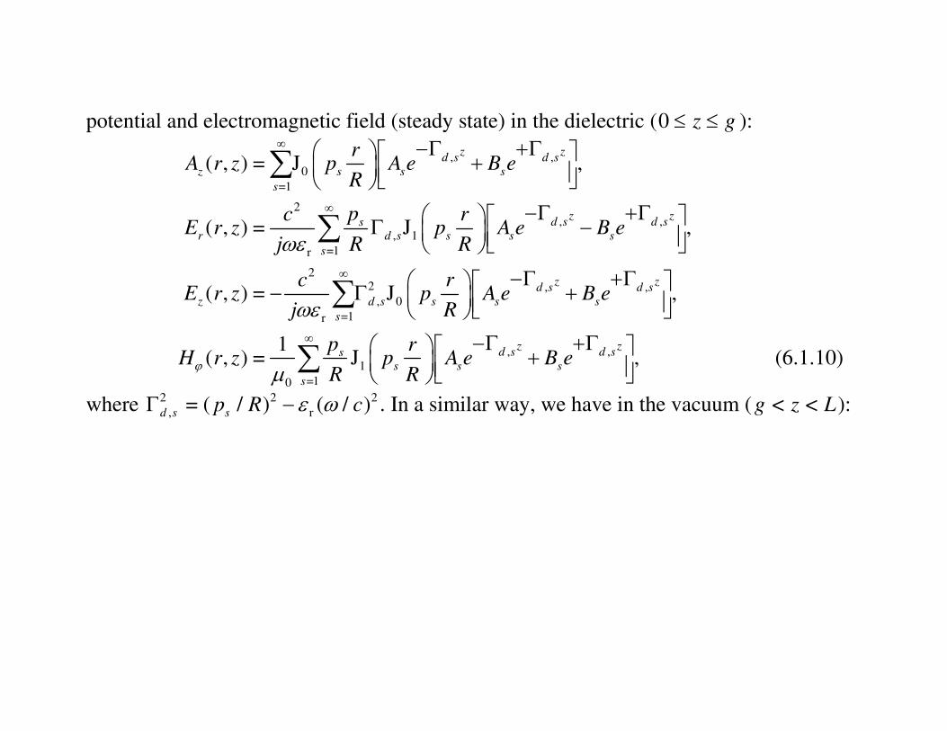
potential and electromagnetic field (steady state) in the dielectric (0 ≤ ≤z g ):
, ,0
=1
2
, ,, 1
=1r
22 , ,
, 0
=1r
1
=10
( , ) = J ,
( , ) = J ,
( , ) = J ,
1( , ) = J
∞
∞
∞
∞
−Γ +Γ +
−Γ +Γ Γ −
−Γ +Γ − Γ +
∑
∑
∑
∑
z zd s d s
z s s s
s
z zd s d ss
r d s s s s
s
z zd s d s
z d s s s s
s
s
s
rA r z p A e B e
R
pc rE r z p A e B e
j R R
c rE r z p A e B e
j R
pH r z p
Rϕ
ωε
ωε
µ, , ,
−Γ +Γ +
z zd s d s
s s s
rA e B e
R (6.1.10)
where 2 2 2
, r= ( / ) ( / )Γ −d s sp R cε ω . In a similar way, we have in the vacuum ( < <g z L):

( ) ( )
0
=1
2( ) ( )
1
=1
2( ) ( )2
0
=1
=10
( , ) = J ,
( , ) = J ,
( , ) = J ,
1( , ) =
∞− −
∞− −
∞− −
∞
−Γ +Γ +
−Γ +Γ Γ −
−Γ +Γ − Γ +
∑
∑
∑
∑
z g z gs s
z s s s
s
z g z gs s sr s s s s
s
z g z gs s
z s s s s
s
s
s
rA r z p C e D e
R
pc rE r z p C e D e
j R R
c rE r z p C e D e
j R
pH r zϕ
ω
ω
µ( ) ( )
1J ,− −−Γ +Γ +
z g z gs s
s s s
rp C e D e
R R (6.1.11)
with 2 2 2
= ( / ) ( / )Γ −s sp R cω . At this point we shall consider only the TM01 mode ( = 1s )
thus the continuity of the radial electric field at =z g implies
[ ],1 ,1,1 1 1 1 1 1
r
1= ,
−Γ +Γ Γ − Γ −
g gd d
d A e B e C Dε
(6.1.12)
and in a similar way the continuity of the azimuthal magnetic field reads
,1 ,1
1 1 1 1= .−Γ +Γ
+ +g g
d dA e B e C D (6.1.13)
Last two equations express the relation between the amplitudes of the field in the
dielectric and vacuum.
In the dielectric filled region of next cell ( ≤ ≤ +L z L g ) the field has a similar form

as in (6.1.10) i.e.,
( ) ( ), ,
0
=1
2( ) ( )
, ,, 1
=1r
2( ) (2 , ,
, 0
=1r
( , ) = J ,
( , ) = J ,
( , ) = J
∞− −
∞− −
∞− −
−Γ +Γ +
−Γ +Γ Γ −
−Γ +Γ − Γ −
∑
∑
∑
z L z L' 'd s d s
z s s s
s
z L z L' 'd s d s
r s d s s s s
s
z L z L' 'd s d s
z d s s s s
s
rA r z p A e B e
R
c rE r z p R p A e B e
j R
c rE r z p A e B e
j R
ωε
ωε)
( ) ( ), ,
1
=10
,
1( , ) = J
∞− −
−Γ +Γ + ∑
z L z L' 'd s d s
s s s s
s
rH r z p R p A e B e
Rϕ µ
(6.1.14)
Accordingly, the boundary conditions at =z L read
( ) ( )
1 1,1 1 1 1 1 1
r
1= ,
− −−Γ Γ Γ − Γ − L g L g' '
d A B C e D eε
(6.1.15)
and
( ) ( )
1 11 1 1 1= .
− −−Γ Γ+ +
L g L g' 'A B C e D e (6.1.16)
The relation between the amplitudes of the wave in the second cell ( < < 2L z L) and
the first cell can be represented in a matrix form

= ,a Ta'
(6.1.17)
where the components of a' are 1
'A and 1
'B and similarly the components of a are 1A and
1B . According to Floquet's theorem (6.1.9) the two vectors are expected to be related by
= ,−
a a' jkL
e (6.1.18)
thus − jkL
e represents the eigen-values of the single cell transmission matrix T :
| |= 0.−−T I
jkLe (6.1.19)
Explicitly this reads
11 22 11 22 12 21
2( ) = 0.
− −− + + −jkL jkLe e T T T T T T (6.1.20)
For a passive system the determinant of the matrix T is unity (prove this statement!!),
thus
11 22
2( ) 1 = 0.
− −− + +jkL jkLe e T T (6.1.21)
The fact that the last term in this equation is unity indicates that if k is a solution of
(6.1.21) −k is also a solution. Consequently, we can write
11 22
1cos( ) = ( ).
2+kL T T (6.1.22)
Note that this is an explicit expression for k as a function of the frequency and the other
geometric parameters. In principle there are ranges of parameters where the right-hand

side is larger than unity and there is no real k which satisfies this relation. If only the
frequency is varied then this result indicates that there are frequencies for which the
solution of the dispersion relation is real thus a wave can propagate, or the solution is
imaginary and the amplitude of the wave is zero. The frequency range for which the wave
is allowed to propagate is called the passband. Explicitly, the right-hand side of (6.1.22)
reads 2 2
1 2 1 2
11 22
1 2 1 2
( ) ( )1( ) = cosh( ) cosh( ),
2 4 4
+ −+ + − −
Z Z Z ZT T
Z Z Z Zψ χ ψ χ (6.1.23)
where 1= ( )Γ −L gψ , ,1= Γd gχ , the characteristic impedances are
0 ,1 0 1
1 2
r
= , = ,Γ Γdc c
Z Zj j
η ηωε ω
(6.1.24)
and 0 = 377Ωη is the impedance of the
vacuum.
0 5 10 15 20 25-2
-1
0
1
2
( )zGHf0.0 0.4 0.80
5
10
20
π/kL
15
()
GH
zf

Figure 2 illustrates the right-hand side of (6.1.22) as a function of the frequency
( r = 10, = 2Rε cm, = 1L cm and = / 2g L ). The blocks at the bottom, illustrate the
forbidden frequencies, namely at these frequencies TM waves can not propagate. In
Figure 3 the dispersion relation of the first three passbands is presented; these branches
correspond only to the TM01 mode. Higher symmetric or asymmetric modes have
additional contributions in this range of frequencies.
Comment 1. The expression in (6.1.22) is the dispersion relation of a TM01 mode in the
periodic structure illustrated in Figure 1. From this simple example however we observe
that the dispersion relation of a periodic structure is itself periodic in k with a
periodicity 2 / Lπ . This is a general feature which can be deduced from (6.1.9). If the
latter is satisfied for 0=k k then (6.1.9) is satisfied also for 0= 2 /+k k Lπ as shown next
2 / )0 0
0
( 2( ) = ( ) ,
= ( ) = ( ).
++ +
+
L L L
L
j k jk jf z L e f z L e e
jkf z L e f z
π π
(6.1.25)
Consequently, since the dispersion relation is periodic in k , it is sufficient to represent
its variation with k in the range / /− ≤ ≤L k Lπ π ; this k domain is also called the first
Brillouin zone.
Comment 2. Bearing in mind the last comment, we can re-examine the expression in

(6.1.8) and realize that ( )f z is represented by a superposition of spatial harmonics
exp( )− njk z where
2
= ,+nk k nL
π (6.1.26)
which all correspond to the solution of the dispersion relation of the system. According
to this definition the phase velocity of each harmonic is
p , = ,h n
n
vck
ω (6.1.27)
and for a high harmonic index, n , this velocity decreases as 1−n . Furthermore, all
harmonics with negative index correspond to backward propagating waves. In addition,
note that the zero harmonic ( = 0n ) has a positive group velocity for / > > 0L kπ and
negative in the range / < < 0− L kπ . This is a characteristic of all spatial harmonics.
Since the group velocity is related to the energy velocity, one can conclude that although
the the wave number of a particular space harmonic is positive, the power it carries may
flow in the negative direction (if the group velocity is negative).

6.2 Closed Periodic Structure
Based on what was shown in the previous section
one can determine the dispersion relation of a TM01
mode which propagates in a corrugated waveguide
[Brillouin (1948)]. Its periodicity is L , the inner
radius is denoted by intR and the external by extR ; the
distance between two cavities (the drift region) is d . Using Floquet's Theorem (6.1.8)
we can write for the magnetic potential in the inner cylinder ( int0 < <r R ) the following
expression
0
=
( , ) = I ( ),∞
−∞
−Γ∑ z
nz n n
n
jkA r z A e r (6.2.1)
and accordingly, the electromagnetic field components read
extR2 int2RL
d

2
1
=
22
0
=
1
=0
( , ) = ( ) I ( ),
( , ) = ( ) I ( ),
1( , ) = I ( )
∞
−∞
∞
−∞
∞
−∞
−− Γ Γ
−−Γ Γ
−− Γ Γ
∑
∑
∑
zn
r n n n n
n
zn
z n n n
n
zn
n n n
n
c jkE r z jk A e r
j
c jkE r z A e r
j
jkH r z A e rϕ
ω
ω
µ (6.2.2)
In these expressions,
2
2 2
2= ,Γ −n nk
c
ω (6.2.3)
and 0 1I ( ), I ( )x x are the zero and first order modified Bessel functions of the first kind
respectively. This choice of the radial functional variation is dictated by the condition of
convergence of the electromagnetic field on axis.
In each individual groove (superscript σ ) the electromagnetic field can be derived
from the following magnetic vector potential:
[ ]( ) ( )
0,
=0
( , ) = cos ( ) ( ),∞
− −∑zA r z B q z z d t rσ σ
ν ν σ νν
(6.2.4)
where = / ( )−q L dν πν ,
0, 0 0 ext 0 0 ext( ) = I ( )K ( ) K ( )I ( ),Λ Λ − Λ Λt r r R r Rν ν ν ν ν (6.2.5)
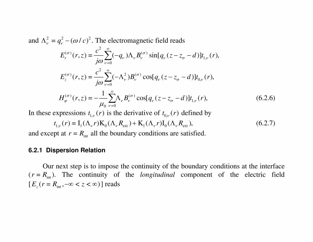
and 2 2 2
= ( / )Λ −q cν ν ω . The electromagnetic field reads
2( ) ( )
1,
=0
2( ) 2 ( )
0,
=0
( ) ( )
1,
=00
( , ) = ( ) sin[ ( )] ( ),
( , ) = ( ) cos[ ( )] ( ),
1( , ) = cos[ ( )] ( ),
∞
∞
∞
− Λ − −
−Λ − −
− Λ − −
∑
∑
∑
r
z
cE r z q B q z z d t r
j
cE r z B q z z d t r
j
H r z B q z z d t r
σ σν ν ν ν σ ν
ν
σ σν ν ν σ ν
ν
σ σϕ ν ν ν σ ν
ν
ω
ω
µ (6.2.6)
In these expressions 1, ( )t rν is the derivative of 0, ( )t rν defined by
1, 1 0 ext 1 0 ext( ) = I ( )K ( ) K ( )I ( ),Λ Λ + Λ Λt r r R r Rν ν ν ν ν (6.2.7)
and except at int=r R all the boundary conditions are satisfied.
6.2.1 Dispersion Relation
Our next step is to impose the continuity of the boundary conditions at the interface
( int=r R ). The continuity of the longitudinal component of the electric field
[ int( = , < < )−∞ ∞zE r R z ] reads

22
0 int
=
22 ( )
0, int
=0
( ) I ( )
0 for < < ,
=
cos[ ( )] ( ) for < < ,
∞
−∞
∞
−−Γ Γ
+− Λ − − + +
∑
∑
zn
n n n
n
c jkA e R
j
z z z d
cB q z z d t R z d z z L
j
σ σ
σν ν ν σ ν σ σ
ν
ω
ω
(6.2.8)
and the azimuthal magnetic field [ int( = , < < )+ +H r R z d z z Lϕ σ σ ] reads
( )
1 int 1, int
= =00 0
1 1I ( ) = cos[ ( )] ( ).
∞ ∞
−∞
−− Γ Γ − Λ − −∑ ∑z
nn n n
n
jkA e R B q z z d t R
σν ν ν σ ν
νµ µ (6.2.9)
From these boundary conditions the dispersion relation of the structure can be
developed. For this purpose we analyze the solution in the grooves having Floquet's
theorem in mind. The latter implies that the longitudinal electric field in the σ 's groove
has to satisfy the following relation:
2 ( ) 2 ( 1)
0, 1 0,
=0 =0
cos[ ( )] ( ) = cos[ ( )] ( ).jkL
B q z z d t r B e q z L z d t rσ σ
ν ν ν σ ν ν ν ν σ νν ν
∞ ∞+
+Λ − − Λ + − −∑ ∑

(6.2.10)
But by definition 1 =+ −z z Lσ σ therefore, the last expression implies that
( )
.− jkz
B B eσ σ
ν ν (6.2.11)
This result permits us to restrict the investigation to a single cell and without loss of
generality we chose =0 = 0zσ since if we know Bν in one cell, the relation in (6.2.11)
determines the value of this amplitude in all other cells. With this result in mind we
multiply (6.2.8) by z
mjk
e and integrate over one cell; the result is
2 2
, 0 int 0, int
= =0
I ( ) ( ) cos[ ( )],∞ ∞
−∞
Γ Γ Λ −∑ ∑ ∫L z
mn n n m n
dn
jkA L R B t R dze q z dν ν ν ν
ν
δ (6.2.12)
here ,n mδ is the Kroniker delta function which equals 1 if =n m and zero otherwise. We
also used the orthogonality of the Fourier spatial harmonics. We follow a similar
procedure when imposing the continuity of the magnetic field with one difference, (6.2.9)
is defined only in the groove aperture thus we shall utilize the orthogonality of the
trigonometric function cos[ ( )]−q z dν . Accordingly, (6.2.9) is multiplied by
cos[ ( )]−q z dµ and we integrate over < <d z L; the result is
1 int 1, int ,
= =0
I ( ) cos ( ) = ( )( ) ,∞ ∞
−∞
− Γ Γ − Λ − ∑ ∑∫L z
nn n n
dn
jkA R dz q z d e B t R L d gµ ν ν ν µ ν µ
ν
δ
(6.2.13)

where 0 = 1g and 0 = 0.5≠gµ otherwise. It is convenient to define the quantity
[ ],
1( ) cos ( ) ,= −
− ∫L z
nn
d
jkk dz q z d e
L dν νL (6.2.14)
which allows us to write (6.2.12) as
2
0, int ,2=00 int
1( ) ( ) ,
I ( )
∞−= ΛΓ Γ ∑n n
n n
L dA t R k B
LRν ν ν ν
ν
L (6.2.15)
and (6.2.13) as
*
1 int ,
=1, int
1I ( ) ( ).
( )
∞
−∞
= Γ ΓΛ ∑ n n n n
n
B A R kt R g
ν νν ν ν
L (6.2.16)
These are two equations for two unknown sets of amplitudes ( , )nA Bν and the
dispersion relation can be represented in two equivalent ways: One possibility is to
substitute (6.2.16) in (6.2.15) and get
0, int *1 int
, , ,2= =0 1, int0 int
( )I ( )0,
( )I ( )
∞ ∞
−∞
ΛΓ Γ−− =
Γ Γ ∑ ∑m m
n m n m m
m n n
t RRL dA
L t R gR
ν νν ν
ν ν ν
δ L L (6.2.17)
whereas the other possibility is to substitute (6.2.15) in (6.2.16) and obtain

2
0, int *1 int
, , ,
=0 =1, int 0 int
( ) I ( )0.
( ) I ( )
∞ ∞
−∞
Λ Γ−−
Λ Γ Γ ∑ ∑ n
n n
n n n
t R RL dB
L t R g R
µ µν µ ν µ µ
µ ν ν ν
δ L L (6.2.18)
In both cases the dispersion relation is calculated from the requirement that the
determinant of the matrix which multiplies the vector of amplitudes, is zero.
Although the two methods are equivalent, we found that the latter expression is by
far more efficient for practical calculation because of the number of modes required to
represent adequately the field in the groove compared to the number of spatial harmonics
required to represent the field in the inner section. In the case of single mode operation
we found that 1 to 3 modes are sufficient for description of the field in the grooves and
about 40 spatial harmonics are generally used in the inner section. As indicated by these
numbers it will be much easier to calculate the determinant of a 3 3× matrix rather than
40 40× one; we shall quantify this statement later. At this point we shall discuss the
design of a disk-loaded structure assuming that the number modes in the grooves and
harmonics in the inner space are sufficient.
Let assume that we want to determine the geometry of a disk-loaded structure which
enables a wave at 10 GHz to be in resonance with electrons with = 0.9β and the phase
advance per cell is assumed to be = 2 / 3kL π . These two conditions determine the period
of the structure. In our case = 9L mm. There are three additional geometric parameters
to be determined: ext int,R R and d . The last two have

a dominant effect on the width of the passband and for the
lowest mode, the passband increases with increasing intR and
decreases with increasing d . The passband, ∆ω , of a mode sets
a limit on the maximum group velocity as can be seen bearing in
mind that the half width of the first Brillouin zone is = /∆k Lπ .
Consequently, g = / < /∆ ∆ ∆rv k Lω ω π . A solution of the
dispersion relation in (6.2.18) is illustrated the geometry chosen
is: 9L = mm, int = 8R mm and = 2d mm and from the condition
of phase advance per cell of 120o at 10 GHz, we determined,
using the dispersion relation, the value of the external radius to
be ext = 13.96R mm.
6.2.2 Modes in the groove
Therefore, before we conclude this subsection, we shall quantify the effect of higher
modes. The first mode in the groove ( = 0ν ) represents a TEM mode which propagates in
the radial direction. Other modes (TM0, >0ν ) are either propagating or evanescent. The
amplitudes of the magnetic and electric field ( zE ) of the TEM mode are constant at the
groove aperture thus the choice of using a single mode in the groove is equivalent to the
0.0 0.4 0.8
π/kL
mmRext 14=mmR 8int =
mmL 9=mmd 2=
3/2π=kL
9.0=βBeam Line
9
10
11
()
GH
zf
8

average process at the boundary
-- approach usually adopted in
the literature. The Figure
illustrates the dependence of
upper and lower cut-off
frequency on the number of
harmonics used in the
calculation; the number of
modes in the grooves is a
parameter. For the geometry
presented above, the number of
harmonics required is 20 or
larger; typically about 40
harmonics are being used. The
effect of the = 1ν mode is
negligible in this case as seen for both upper and lower cut-off frequencies. The effect of
the higher mode introduces a correction on the order of 1% which for most practical
purposes is sufficient.
0 20 40 60 8010010.0
10.2
10.4
10.6
10.8
11.0
Total Number ofHarmonics
=3
0 20 40 60 80100
Total Number ofHarmonics
8.65
8.67
8.69
8.71
8.73
8.75
()
GH
zf
()
GH
zf
=2Modes=1
=3=2
Modes=1

6.2.3 Spatial Harmonics Coupling
Contrary to uniform dielectric structures, here each mode consists of a superposition
of an infinite number of spatial harmonics. These harmonics are all coupled by the
conditions imposed on the electromagnetic field by the geometry at int=r R . We shall
limit the investigation to the accuracy associated with a single mode taken in the groove,
therefore according to (6.2.15), we have
2
0,0 int ,0 02 2
0 int
1( ) ( ) ,
I ( )= −
Γ Γn n
n n
A t R k BR c
ωL (6.2.19)
and in this particular case
,0
1 1( ) sinc ( ) exp ( ) .
2 2
− = − + n n n
L dk k L d j k L d
LL (6.2.20)
Let us compare the first few spatial harmonics relative to the zero harmonic. For this
purpose we take = 10f GHz, 0 int= 0.9 , = 8v c R mm, = 9L mm and = 2d mm. The ratio
of the first two amplitudes is

3 6 6 81 1 2 2
0 0 0 0
= 8 10 , = 3 10 , = 2 10 , = 1 10A A A A
A A A A
− − − −− −× × × × (6.2.21)
This result indicates that on axis, the amplitude of the interacting harmonic is dominant.
At the interface with the grooves ( int=r R ) the ratio between the contribution of the zero
and n th harmonic is much closer to unity and it can be checked that it reads
, int
,0 int 0
| ( = ) | | sinc( ( ) / 2) |,
| ( = ) | | sinc( ( ) / 2) |
−=
−z n n
z
E r R k L d
E r R k L d (6.2.22)
which is a virtually unity.
A more instructive picture is obtained by examining the average power flowing in
one time and spatial period of the system:
int *
0 0
1 1= 2 ( , ) ( , ) .
2
∫ ∫
R L
rP drr dz E r z H r zL
ϕπ (6.2.23)
According to the definition in (6.2.2) we have
int2 2
10
=0
| | I ( );∞ Γ
−∞
= ∑ ∫R
nn
n
n
ckP cA dxx x
πη ω
(6.2.24)
the integral can be calculated analytically [Abramowitz and Stegun (1968) p.484] and it
reads

2 2 2 2
1 0 1 1 00
1( ) I ( ) I ( )I ( ) [I ( ) I ( )].
2≡ + −∫U dxx x
ξξ ξ ξ ξ ξ ξ ξ (6.2.25)
Based on these definitions we can calculate the average power carried by each harmonic
as
2
int
0
| | ( ),= Γn
n n n
ckP cA U R
πη ω
(6.2.26)
and the result is listed below
3 4 32 1 1 2
0 0 0 0
= 3 10 , = 0.16, = 1 10 , = 3 10P P P P
P P P P
− − −− −− × − × × (6.2.27)
Although there is a total flow of power along (the positive) direction of the z axis, a
substantial amount of power is actually flowing backwards. In this numerical example for
all practical purposes we can consider only the lowest two harmonics and write the total
power which flows, normalized to the power in the zero harmonic. Thus if the latter is
unity, then the power in the forward is 1 0.16 = 0.84− . This result indicates that if we
have a finite length structure with finite reflections from the input end, then in this
periodic structure we have an inherent feedback even if the output end is perfectly
matched.

6.3 Open Periodic Structure
In this section an analysis similar to
that in Section 6.2 is applied to an open
periodic structure. As we shall see the
number of modes which may develop in
such a structure is small and therefore
mode competition is minimized.
We shall consider a system in which the wave propagates along the periodic
structure which consists of a disk-loaded wire, as illustrated in Figure 5 whose periodicity
is L , the inner radius is denoted by intR , the external by extR and the distance between two
cavities is d . Floquet's theorem as formulated in (6.1.8) allows us to write for the
magnetic potential in the external region ( ext>∞ ≥r R ) the following expression
0
=
( , ) = K ( ),∞
−∞
−Γ∑ z
nz n n
n
jkA r z A e r (6.3.1)
and accordingly, the electromagnetic field components read
extR2
d
int2RL

2
1
=
22
0
=
1
=0
( , ) = ( ) K ( ),
( , ) = ( ) K ( ),
1( , ) = ( ) K ( )
zn
r n n n n
n
zn
z n n n
n
zn
n n n
n
c jkE r z jk A e r
j
c jkE r z A e r
j
jkH r z A e rϕ
ω
ω
µ
∞
−∞
∞
−∞
∞
−∞
−Γ Γ
−−Γ Γ
−− −Γ Γ
∑
∑
∑
(6.3.2)
In these expressions 0 1K ( ), K ( )x x are the zero and first order modified Bessel functions
of the second kind respectively and 2 2 2
= ( / )Γ −n nk cω . This choice of the radial functional
variation is dictated by the condition of convergence of the electromagnetic field far
away from the structure.
In each individual groove the electromagnetic field can be derived from the
following magnetic vector potential:
( ) ( )
0,
=0
( , ) = cos[ ( )] ( ),∞
− −∑zA r z B q z z d t rσ σ
ν ν σ νν
(6.3.3)
where = / ( )−q L dν πν ,
0, 0 0 int 0 0 int( ) = I ( )K ( ) K ( )I ( ),Λ Λ − Λ Λt r r R r Rν ν ν ν ν (6.3.4)
and 2 2 2
= ( / )Λ −q cν ν ω . The electromagnetic field reads

2( ) ( )
1,
=0
2( ) 2 ( )
0,
=0
( ) ( )
1,
=00
( , ) = ( ) sin[ ( )] ( ),
( , ) = ( ) cos[ ( )] ( ),
1( , ) = cos[ ( )] ( ).
∞
∞
∞
− Λ − −
−Λ − −
− Λ − −
∑
∑
∑
r
z
cE r z q B q z z d t r
j
cE r z B q z z d t r
j
H r z B q z z d t r
σ σν ν ν ν σ ν
ν
σ σν ν ν σ ν
ν
σ σϕ ν ν ν σ ν
ν
ω
ω
µ (6.3.5)
The index σ labels the ``cavity" and in these expressions we used
1, 1 0 int 1 0 int( ) = I ( )K ( ) K ( )I ( ).Λ Λ + Λ Λt r r R r Rν ν ν ν ν (6.3.6)
The solution above satisfies all boundary conditions with the exception of ext=r R .
6.3.1 Dispersion Relation
Our next step is to impose the continuity of the boundary conditions at the interface
( ext=r R ). Continuity of the longitudinal component of the electric field implies
ext( = , < < )−∞ ∞zE r R z , reads

22
0 ext
=
22 ( )
0, ext
=0
( ) K ( )
0 for < < ,
cos[ ( )] ( ) for < < ,
∞
−∞
∞
−−Γ Γ =
+− Λ − − + +
∑
∑
zn
n n n
n
c jkA e R
j
z z z d
cB q z z d t R z d z z L
j
σ σ
σν ν ν σ ν σ σ
ν
ω
ω
(6.3.7)
and the azimuthal magnetic field, ext( = , < < )+ +H r R z d z z Lϕ σ σ , reads
( )
1 ext 1, ext
= =00 0
1 1K ( ) cos[ ( )] ( ).
∞ ∞
−∞
−Γ Γ − Λ − −∑ ∑z
nn n n
n
jkA e R B q z z d t R
σν ν ν σ ν
νµ µ (6.3.8)
Following the same arguments as in Section 6.2.1 it can be shown that
( )=
− jkzB B e
σ σν ν and consequently we can limit the discussion to a single cell. We
multiply (6.3.7) by z
mjk
e and integrate over one cell; the result being
2 2
, 0 ext 0, ext
= =0
K ( ) ( ) cos[ ( )].∞ ∞
−∞
Γ Γ Λ −∑ ∑ ∫L z
mn n n m n
dn
jkA L R B t R dze q z dν ν ν ν
ν
δ (6.3.9)

We follow a similar procedure when imposing the continuity of the magnetic field; the
difference in this case is that (6.3.8) is defined only in the groove's aperture thus we shall
utilize the orthogonality of the trigonometric function cos[ ( )]−q z dν . Accordingly,
(6.3.8) is multiplied by cos[ ( )]−q z dµ and we integrate over < <d z L; the result is
1 ext 1, ext ,
= =0
K ( ) cos[ ( )] ( )( ) .∞ ∞
−∞
−Γ Γ − − Λ −∑ ∑∫
L zn
n n nd
n
jkA R dz q z d e B t R L d gµ ν ν ν µ ν µ
ν
δ
(6.3.10)
In this expression 0 = 1g and 0 = 0.5≠ng . It is convenient to define the quantity
,
1( ) cos[ ( )] ,= −
− ∫L z
nn
d
jkk dz q z d e
L dν νL (6.3.11)
by whose means, (6.3.9) reads
2
0, ext ,2=00 ext
1( ) ( ) ,
K ( )
∞−= ΛΓ Γ ∑n n
n n
L dA t R k B
LRν ν ν ν
ν
L (6.3.12)
whereas (6.3.10)
*
1 ext ,
=1, ext
1K ( ) ( ).
( )
∞
−∞
− Γ ΓΛ ∑ n n n n
n
B A R kt R g
ν νν ν ν
L (6.3.13)
These are two equations for two unknown sets of amplitudes ( , )nA Bν . The

dispersion relation can be represented in two equivalent ways: One possibility is to
substitute (6.3.13) in (6.3.12) and obtain one equation for the amplitudes of the various
harmonics
0, ext *1 ext
, , ,2= =0 1, ext0 ext
( )K ( )= 0.
( )K ( )
∞ ∞
−∞
ΛΓ Γ−+
Γ Γ ∑ ∑m m
n m n m m
m n n
t RRL dA
L t R gR
ν νν ν
ν ν ν
δ L L (6.3.14)
The other possibility is to substitute (6.3.12) in (6.3.13) and obtain one equation for the
amplitudes of the various modes in the groove 2
0, ext *1 ext
, , ,
=0 =1, ext 0 ext
( ) K ( )= 0.
( ) K ( )
∞ ∞
−∞
Λ Γ−+
Λ Γ Γ ∑ ∑ n
n n
n n n
t R RL dB
L t R g R
µ µν µ ν µ µ
µ ν ν ν
δ L L (6.3.15)
In both cases the dispersion relation is calculated from the requirement that the
determinant of the matrix which multiplies the vector of amplitudes, is zero. As in the
closed structure the two methods are equivalent, but the last expression is by far more
efficient for practical calculation.
There is one substantial difference between open and closed periodic structures. In the
latter case, the radiation is guided by the waveguide and there is an infinite discrete
spectrum of frequencies which can propagate along the system. In open structures, modes
can propagate provided that the projection of the wavenumbers of all harmonics in the
first Brillouin zone corresponds to waves whose phase velocity is smaller than c ; in other

words, no radiation propagates outwards
(radially). The figure illustrates the two
regions of interest: in the shadowed region no
solutions are permissible and in the remainder
the solution is possible with an adequate
choice of the geometric parameters. It is
evident from this picture that waves at
frequencies higher than
1
,2
≥c
fL
(6.3.16)
can not be supported by a disk-loaded wire, regardless of the
geometrical details of the cavity. With this regard, an open
structure forms a low pass filter. Figure 3.1 illustrates the
dispersion relation of such a system for = 3L mm, = 1d mm,
int = 15R mm and ext = 21R mm. For comparison, in the same
frequency range (0--50 GHz) there are 6 symmetric TM modes
which can propagate in a closed system of the same geometry;
obviously there are many others at higher frequencies.
ω
π/kL-6 0 2 4
1=phβ 1=phβ
-2-4
π/kL
0.0 0.2 0.4 0.6 0.8 1.0
mmR 15int =mmRext 21=
mmL 3=mmd 1=
0
10
20
30
40
50
()
GH
zf
1=phβ

6.4 Transients
In order to illustrate the effect of the periodicity on the propagation of a wave packet
we shall consider at = 0t the same wavepacket ( )a z , in vacuum and in a periodic
structure. The propagation in vacuum will be represented by a dispersion relation 2 2 2= /k cω , therefore a scalar wave function ( , )Ψ z t is given by
1
( , ) = ( ) .2
∞
−∞
− − Ψ + ∫jkz jkct jkct
z t dk k e e eψ (6.4.1)
Since at = 0t this function equals ( )a z , the amplitudes ( )kψ can be readily determined
using the inverse Fourier transform hence
1
( ) = ( ) .2
∞
−∞∫jkz
k dza z eψπ
(6.4.2)
Substituting back into (4.1) we find that
[ ]1( , ) = ( ) ( ) ,
2Ψ − + +z t a z ct a z ct (6.4.3)
which basically indicates that the pulse moves at the speed of light in both directions and
asymptotically, it preserves its shape. In a periodic structure the description of the
wavepacket is complicated by the dispersion relation which in its lowest order
approximation (e.g., first TM symmetric mode in a waveguide) can be expressed as

( ) = cos( ),−k kLω ω δω (6.4.4)
where 0= ( ) / 2+ πω ω ω is the average frequency between the low ( = 0kL ) cut-off
denoted by 0ω and the high ( =kL π ) cut-off denoted by πω . The quantity
0= ( ) / 2−πδω ω ω is half the passband width and L is the period of the structure.
Contrary to the previous case k here denotes the wavenumber in the first Brillouin zone.
In the framework of this approximation we can use Floquet's representation to write
/
/=
( )( , ) = Re ( ) ,
∞
−−∞
−Ψ
∑ ∫
L zn
nL
n
j k t jkz t dk k e
π
π
ωψ (6.4.5)
where = 2 /+nk k n Lπ . The amplitudes ( )n kψ are determined by the value of the
function at = 0t hence
( ) = 12 ( ) .∞
−∞∫z
nn
jkk dza z eψ π (6.4.6)
Substituting back into (6.4.5) we have
/ ( )
/=
1 [ cos( )]( , ) = Re ( ) .
2
∞∞ −
−∞ −−∞
− −Ψ
∑∫ ∫
L zn
Ln
jt kL jkz t d a dke
π ζ
π
ω δωζ ζπ
(6.4.7)
At this point we can take advantage of

=
1( 1/ )
2 J ( ),∞
−∞
−≡ ∑e
νν
ν
ζ τ ττ ζ (6.4.8)
and simplify the last equation to read
/ ( )
/= =
1 ( /2)( , ) = Re ( ) J ( ) ,
2
∞ ∞∞ −
−∞ −−∞ −∞
−−Ψ ×
∑ ∑∫ ∫L z
n
Ln
jkj t j kLz t d a dke t e e
π ζνπ
ν
ω π νζ ζ δωπ
(6.4.9)
which after the evaluation of the integrals and summation (over n ) reads
=
( , ) = ( )J ( )cos( / 2).∞
−∞
Ψ − −∑z t a z L t tνν
ν δω ω πν (6.4.10)

The figure illustrates the propagation of two
wavepackets in vacuum (dashed line) and in a
periodic structure. The latter is characterized by
= 2 10×ω π GHz, = / 30δω ω and a spatial
periodicity of = 1L cm. At = 0t the distribution is a
Gaussian, 2( ) = exp[ ( / ) ]−a z z L . In each one of the
frames ( , )Ψ z t was plotted at a different time as a
function of z . Characteristic to all the frames is the
relatively large peak following the front of the pulse.
It is evident that although the front of the pulse
propagates at the speed of light (as in vacuum) the
main pulse propagates slower. In fact, a substantial
fraction of the energy remains at the origin even a
long time after = 0t . For the parameters used, the
amplitude of the signal at the origin ( = 0z ) is
dominated by the zero order Bessel function i.e.,
0J ( )tδω therefore the energy is drained on a time
scale which is determined by the asymptotic behavior
of the Bessel function namely 1 /∝ tδω . Clearly the wider the passband the faster the
energy is drained from the origin.
0 5 10 15-0.5
0.0
0.5
Lz /
()t
z,Ψ
cLt /12=
cLt /3= cLt /6=
cLt /9=
0 5 10 15-0.5
0.0
0.5
Lz /
()t
z,Ψ
0 5 10 15-0.5
0.0
0.5
Lz /
()t
z,Ψ
0 5 10 15-0.5
0.0
0.5
Lz /
()t
z,Ψ
Exercise 6.1: Based on the solution for ( , )zA r z in Section 6.1 determine the Floquet
representation of the magnetic vector potential (TM01). In other words write
0 1( , ) = J ( )−
∑ zn
z n
n
r jkA r z p a k e
R
and determine ( )na k .
Exercise 6.2: Find all the waves which can propagate between = 0f to 20 GHz,
including asymmetric modes for the system described in Section 6.1. Repeat this exercise
for the branches of the TE modes.
Exercise 6.3: Analyze the coupling of spatial harmonics for the system in Section 6.3 in
a similar way as in Section 6.2.2.
Exercise 6.4: Repeat the calculation of the propagation of a transient in a periodic
structure (Section 6.4) but this time for a TEM-like mode. [Hint: take = ( )∼ khπω ω .]

Chapter 7: Generation of radiation
Throughout these notes it was always assumed that somewhere there is a radiation source
providing us with the necessary energy. In what follows we shall skim through the
fundamentals of generation of radiation. Our discussion will be limited to ``vacuum''
devices, this is to say that the energy is extracted from free electrons in vacuum.
Employed on medium (< 1kW) and high (> 1kW) power devices, the concepts to be
discussed rely solely on energy and momentum conservation. Another very important
family of devices relying on electrons moving in ``solid state'', will not be discussed here.
7.1 Single-Particle Interaction
On its own, an electron cannot transfer energy via a linear process to a
monochromatic electromagnetic wave in vacuum if the interaction extends over a very
long region. Non-linear processes may facilitate energy exchange in vacuum, but this
kind of mechanism is rarely used since most systems require a linear response at the
output. Therefore throughout this text we shall consider primarily linear processes and in
this introductory chapter we shall limit the discussion to single-particle schemes.
Collective effects, where the current is sufficiently high to affect the electromagnetic
field, are also important but cannot be covered at this stage and they are the essence of a
different course.
7.1.1 Infinite Length of Interaction
Far away from its source, in vacuum, an electromagnetic wave forms a plane wave
which is characterized by a wavenumber whose magnitude equals the angular frequency,
ω , of the source divided by 1
= 299,792,458m−
c s , the phase velocity of the plane wave
in vacuum, and its direction of propagation is perpendicular to both the electric and
magnetic field. For the sake of simplicity let us assume that such a wave propagates in
the z direction and the component of the electric field is parallel to the x axis i.e.,

0( , ) = cos . −
x
zE z t E t
cω (7.1.1)
If a charged particle moves at v parallel to z axis, then the electric field this charge
experiences (neglecting the effect of the charge on the wave) is given by
0
( )( ( ), ) = cos .
− x
z tE z t t E t
cω (7.1.2)
A crude estimate for the particle's trajectory is
( ) ,z t vt (7.1.3)
therefore if the charge moves in the presence of this wave from → −∞t to →∞t then
the average electric field it experiences is zero,
cos 1 = 0,∞
−∞
− ∫
vdt t
cω (7.1.4)
even if the particle is highly relativistic. The lack of interaction can be illustrated in a
clearer way by superimposing the dispersion relation of the wave and the particle on the
same diagram. Firstly, the relation between energy and momentum for an electron is
given by
2 2= ( ) ,+E c p mc (7.1.5)
where 31= 9.1094 10−×m Kg is the rest mass of the electron. Secondly, the corresponding

relation for a photon in free space is
= .E cp (7.1.6)
For the interaction to take place the electron has to change its initial state, subscript i,
denoted by i i( , )E p along the dispersion relation to the final, subscript f, denoted by
f f( , )E p in such a way that the resulting photon in case of emission or absorbed photon
for absorption, has exactly the same difference of energy and momentum i.e.,
i f ph= ,+E E E (7.1.7)
and
i f ph= .+p p p (7.1.8)
In vacuum this is impossible, as can be shown by
substituting (7.1.5)--(7.1.6)in (7.1.7)--(7.1.8). We
can also reach the same conclusion by examining
Fig. 1.1 The expression, =E cp , which describes
the photon's dispersion relation, is parallel to the
asymptote of the electron's dispersion relation. Thus,
if we start from one point on the latter, a line parallel
to =E cp will never intersect (7.1.5) again. In other
words, energy and momentum can not be conserved
simultaneously in vacuum.
p
iE
E
222 cmpcE +=
cpE =
ip
E
fp
f

7.1.2 Finite Length of Interaction
If we go back to (7.1.4) we observe that if the electron spends only a finite time in the
interaction region then it can experience a net electric field. Let us denote by −T the time
the electron enters the interaction region and by T the exit time. The average electric
field experienced by the electron (subject to the same assumptions indicated above) is
( )0
0
1= cos 1 ,
2
= sinc 1 ;
−⟨ ⟩ −
−
∫T
TE E dt t vc
T
vE T
c
ω
ω (7.1.9)
here sinc( ) = sin( ) /x x x . That is to say that if the time the electron spends in the
interaction region, is small on the scale of the radiation period 0 = 2 /T π ω then the net
electric field it experiences, is not zero. From the perspective of the conservation laws,
the interaction is possible since although the energy conservation remains unchanged i.e.,
i f= ,+ E E ω (7.1.10)
the constraint on momentum conservation was released somewhat and it reads

i f| |< ,− − p p cTc
ω (7.1.11)
which clearly is less stringent than in (7.1.8) as also illustrated
in the figure; 34
= 1.05457 10 Jsec−× is the Planck constant. The
operation of the klystron to be discussed subsequently relies on
the interaction of an electron with a wave in a region which is
shorter than the radiation wavelength.
7.1.3 Finite Length Pulse
Another case where energy transfer is possible in vacuum is when the pulse duration
is short. In order to examine this case we consider, instead of a periodic wave whose
duration is infinite, a short pulse of a typical duration τ . In order to visualize the
configuration, consider a field given by 2 2( / ) /
0( , ) = .− −t z c
xE z t E eτ
(7.1.12)
A particle following the same trajectory as in (7.1.3) will clearly
experience an average electric field which is non-zero even when
the interaction duration is infinite. This is possible since the
spectrum of the radiation field is broad -- in contrast to Sect. 7.1.1
where it was peaked -- therefore again the constraint of the
conservation laws is less stringent:
p
iE
E
222 cmpcE +=
ip
E
cpE =
fp
f
iE
fE
222cmpcE +=
E
cpE =
fppip

i f| |< ,−
E Eτ
(7.1.13)
and
i f| |< .−
p pcτ
(7.1.14)
Schematics of this mechanism is illustrated in the figure. It should be also pointed out
that in this section we consider primarily the kinematics of the interaction and we pay no
attention to the dynamics. In other words, we examined whether the conservation laws
can be satisfied without details regarding the field configuration.
7.1.4 Cerenkov Interaction
It was previously indicated that since the dispersion
relation of the photon is parallel to the asymptote of the
electron's dispersion relation, the interaction is not possible
in an infinite domain. However, it is possible to change the
``slope'' of the photon, namely to change its phase velocity
-- see Figure. The easiest way to do so is by ``loading" the
medium where the wave propagates with a material whose
dielectric coefficient is larger than one. Denoting the
p
222 cmpcE +=
ip
cpE =
fp
( )pncE /=
iE
E
fE

refraction coefficient by n , the dispersion relation of the photon is given by
ph ph= ,c
E pn
(7.1.15)
while the dispersion relation of the electron remains unchanged. Substituting in the
expressions for the energy and the momentum conservation laws we find that the
condition for the interaction to occur is
= ,c
vn
(7.1.16)
where it was assumed that the electron's recoil is relatively small i.e., 2/ 1 mcω . The
result in (7.1.16) indicates that for the interaction to occur, the phase velocity of a plane
wave in the medium has to equal the velocity of the particle. This is the so-called
Cerenkov condition. Although dielectric loading is conceptually simple, it is not always
practical because of electric charges which accumulate on the surface and of a relatively
low breakdown threshold which is critical in high-power devices. For these reasons the
phase velocity is typically slowed down using metallic structures with periodic
boundaries. The operation of traveling wave tubes (or backward wave oscillators) relies
on this concept.

7.1.5 Compton Scattering: Static Fields
It is not only a structure with periodic boundaries
which facilitates the interaction between electrons and
electromagnetic waves but also periodic fields. For example,
if a magneto-static field of periodicity L is applied on the
electron in the interaction region, then this field serves as a
momentum ``reservoir" which can supply momentum quanta of (2 / )n Lπ where
= 0, 1, 2,...± ±n ; see Figure. The energy conservation law remains unchanged i.e.,
i f ph= ,+E E E (7.1.17)
but the momentum is balanced by the applied static field
i f ph
2= .+ + p p p n
L
π (7.1.18)
For a relativistic particle ( 1)β and when the electron's recoil is assumed to be small,
these two expressions determine the so-called resonance condition which reads
2 22 ,
c
nL
πω γ (7.1.19)
where 2 1/2[1 ( / ) ]−≡ − v cγ . Note that the frequency of the emitted photon depends on the
p
iE
222cmpcE +=
ip
E
cpE =fE
Lnh /
fp

velocity of the electron which means that by varying the velocity we can change the
operating frequency. A radiation source which possesses this feature is a tunable source.
Identical result is achieved if we assume a periodic electrostatic field and both field
configurations are employed in the so-called ``free electron lasers''.
7.1.6 Compton Scattering: Dynamic Fields
Static electric or magnetic field can be conceived as limiting cases of a dynamic
field of zero or vanishingly small frequency and we indicated above that they facilitate
the interaction between an electron and a wave. Consequently we may expect that the
interaction of an electron with a wave will occur in the presence of another wave. Indeed,
if we have an initial wave of frequency 1ω and the emitted wave is at a frequency 2ω the
conservation laws read
i 1 f 2= ,+ + E Eω ω (7.1.20)
and
1 2
i f= .+ + p pc c
ω ω (7.1.21)
Following the same procedure as above we find that the ratio between the frequencies of
the two waves is

22
1
4 ,ω
γω
(7.1.22)
which is by a factor of 2 larger than in the static case. The figure
illustrates this process.
7.1.7 Uniform Magnetic Field
A periodic magnetic field can provide quanta of momentum necessary to satisfy the
conservation law. It does not affect the average energy of the particle. An opposite
situation occurs when the electron moves in a uniform magnetic field (B ): there is no
change in the momentum of the particle whereas its energy is given by
2 2= ( ) 2 ,+ − E c p mc n eB (7.1.23)
where 19= 1.6022 10−×e C is the charge of the electron and = 0, 1, 2...± ±n .
For most practical purposes the energy associated with the magnetic field is much
smaller than the energy of the electron therefore we can approximate
p
iE
ip
E
cpE =fE
fp
222 cmpcE +=
1E
2E

2 2
i 1 f 2 ph
i f
= ,− − + ec B ec B
E n E n EE E
(7.1.24)
and the momentum conservation remains unchanged i.e.,
i f ph= .+p p p (7.1.25)
From these two equations we find that the frequency of the
emitted photon is
2
= 2 = 2 .
eB eB
m mω γ γ
γ (7.1.26)
The last term is known as the relativistic cyclotron angular frequency, c, /≡rel eB mω γ .
The figure illustrates schematically this type of interaction. It indicates that the dispersion
line of the electron is split by the magnetic field in many lines (index n ) and the
interaction is possible since the electron can move from one line to another. Gyrotron's
operation relies on this mechanism and it will be discussed briefly in the next section.
7.1.8 Synchronism Condition
All the processes in which the interaction of an electron with a monochromatic wave
extends to large regions, have one thing in common: the velocity of the electron has to
p
E
cpE =
fE
fp ip
iE
1+n
n
1−n
π2/2222neBhcmpcE −+=

equal the effective phase velocity of the pondermotive wave along the electron's main
trajectory, namely
ph,eff= .v v (7.1.27)
Here by pondermotive wave we mean the effective wave along the longitudinal trajectory
of the particle which accounts for transverse or longitudinal oscillation. In the Cerenkov
case we indicated that the phase velocity is /c n and there is no transverse motion
therefore the condition for interaction implies = /n c v where n is the refraction
coefficient of the medium. In the presence of a periodic static field the wavenumber of
the pondermotive wave is / 2 /+c Lω π therefore
ph,eff = ,/ 2 /+
vc L
ωω π
(7.1.28)
and for a dynamic field
2 1
ph,eff
2 1
= ,−
+v
k k
ω ω (7.1.29)
where 1,2 1,2= /k cω are the wavenumbers of the two waves involved. Finally, in a
uniform magnetic field only the effective frequency varies
c,rel
ph,eff = .−
vk
ω ω (7.1.30)
The reader can check now that within the framework of this formulation we obtain

(7.1.19) from (7.1.28), in the case of the dynamic field we have from (7.1.29) the 24γ
term as in (7.1.22) and finally (7.1.30) leads to the gyrotron's operation frequency
presented in (7.1.26).

7.2 Radiation Sources: Brief Overview
There are numerous types of radiation sources driven by electron beams. Our
purpose in this section is to continue the general discussion from the previous section and
briefly describe the operation principles of one ``member" of each class of what we
consider the main classes of radiation sources. A few comments on experimental work
will be made and for further details the reader is referred to recent review studies. The
discussion continues with the classification of the major radiation sources according to
several criteria which we found to be instructive.
7.2.1 The Klystron
The klystron was one of the first radiation sources to be developed. It is a device in
which the interaction between the particle and the wave is localized to the close vicinity
of a gap of a cavity, as illustrated in the Figure.
input
output
cathode
collector

Electrons move along a drift tube and its geometry is chosen in such a way that at
the frequency of interest it does not allow the electromagnetic wave to propagate. The
latter is confined to cavities attached to the drift tube. The wave which feeds the first
cavity modulates the velocity of the otherwise uniform beam. This means that after the
cavity, half of the electrons have a velocity larger than the average beam velocity
whereas the second half has a smaller velocity. According to the change in the (non-
relativistic) velocity of the electrons the beam becomes bunched down the stream since
accelerated electrons from one period of the electromagnetic wave catch up with the slow
electrons from the previous period. When this bunch enters the gap of another cavity it
may generate radiation very efficiently. In practice, several intermediary cavities are
necessary to achieve good modulation.
7.2.2 The Traveling Wave Tube
The traveling wave tube (TWT) is a Cerenkov device, namely the phase velocity of
the interacting wave is smaller than c and the interaction is distributed along many
wavelengths. Generally speaking, as the beam and the wave advance, the beam gets
modulated by the electric field of the wave and in turn, the modulated beam increases the
amplitude of the electric field. In this process both the beam modulation and the radiation
field grow exponentially in space.

input
output
cathode
input output
cathode
collector
(a)
(b)
output
input
cathode output
cathode
(c)
(d)
(e)
cathode

In the interaction process the electron oscillates primarily along the major axis ( z
direction ) and the interaction is with the parallel component of the electric field.
Correspondingly, the interaction occurs here with the transverse magnetic (TM) mode.
7.2.3 The Gyrotron
The gyrotron relies on the interaction between an annular beam, gyrating around the
axis of symmetry due to an applied uniform magnetic field, and a transverse electric (TE)
mode. The concept of generating coherent radiation from electrons gyrating in a magnetic
field was proposed independently by three different researchers in the late fifties, and it
has attracted substantial attention due to its potential to generate millimeter and
submillimeter radiation.
In this device electrons move in the azimuthal direction and they get bunched by the
corresponding azimuthal electric field. As in the case of the TWT the bunches act back
on the field and amplify it. In contrast to traveling wave tubes or klystrons in which the
beam typically interacts with the lowest mode, in the gyrotron the interaction is with high
modes therefore various suppression techniques are employed in order to obtain coherent
operation with a single mode.
The operation frequency is determined by the applied magnetic field, the energy of
the electrons and, in cases of high mode operation, also by the radius of the waveguide:

2 2
c c c= ,+ + oω ω γ γβ ω ω (7.2.1)
where = /v cβ , = /c eB mω and coω is the cutoff frequency of the mode. The operating
frequency in this case can reach very high values: for a magnetic field of 1T and 2.5γ
the operation frequency is of the order of 150 GHz or higher according to the mode with
which the electrons interact.
Since the interaction of the electrons is with an azimuthal electric field, it is
necessary to provide the electrons with maximum momentum in this direction. The
parameter which is used as a measure of the injected momentum is the ratio of the
First Anode-350kV
Circuit Coil
Second Anode Open Cavity
Gun Coil
Cathode500kV
transverse to longitudinal momentum /⊥≡ zv vα . This transverse motion is acquired by
the electrons in the gun region as can be deduced from the schematics illustrated in the
Figure. In relativistic devices this ratio is typically smaller than unity whereas in non-
relativistic devices it can be somewhat larger than one.
Beam location is also very important. In the TWT case the interaction is with the
lowest symmetric TM mode. Specifically the electrons usually form a pencil beam and
they interact with the longitudinal electric field which has a maximum on axis. We
indicated that gyrotrons operate with high TE modes and the higher the mode, the higher
the number of nulls the azimuthal electric field has along the radial direction. Between
each two nulls there is a peak value of this field. It is crucial to have the annular beam on
one of these peaks for an efficient interaction to take place.
7.2.4 The Free Electron Laser
As the gyrotron, it is a fast-wave device in the sense that the interacting
electromagnetic wave has a phase velocity larger or equal to c but instead of a uniform
magnetic field it has a periodic magnetic field. The ``conventional" free electron laser
(FEL) has a magnetic field perpendicular to the main component of the beam velocity. As
a result, the electrons undergo a helical motion which is suitable for interaction with
either a TE or a TEM mode. The oscillation of electrons is in the transverse direction but
the bunching is longitudinal and in this last regard the process is similar to the one in the

traveling wave tube. However, its major advantage is the fact that it does not require a
metallic (or other type of) structure for the interaction to take place. Consequently, it has
the potential to either generate very high power at which the contact of radiation with
metallic walls would create very serious problems, or produce radiation at UV, XUV or
X-ray where there are no other coherent radiation sources. The Figure illustrates the basic
configuration.
cathode
N N N NSS S S
N N NSS S S N

7.2.5 The Magnetron
The magnetron was invented at the beginning
of the 20th century but because of its complexity
there is no analytical model, as yet, which can
describe its operation adequately as a whole. In
recent years great progress has been made in the
understanding of the various processes with the aid
of particle in cell (PIC) codes. Its operation combines potential and kinetic energy
conversion. The Figure illustrates the basic configuration. Electrons are generated on the
cathode (inner surface) and since a perpendicular magnetic field is applied they form a
flow which rotates azimuthally. The magnetic field and the voltage applied on the anode
are chosen in such a way that, in equilibrium, the average velocity of the electrons equals
the phase velocity of the wave supported by the periodic structure at the frequency of
interest.
A simplistic picture of the interaction can be conceived in the following way:
electrons which lose energy to the wave via the Cerenkov type interaction, move in
upward trajectories -- closer to the anode. Consequently, two processes occur. Firstly, the
closer the electron is to the periodic surface the stronger the radiation field and therefore
v
B

the deceleration is larger, causing a further motion upwards. Secondly, as it moves
upwards its (dc) potential energy varies. Again, this is converted into electromagnetic
energy.
Two major differences between the magnetron and other radiation sources
mentioned above, are evident: (i) in the magnetron the beam generation, acceleration and
collection occur all in the same region where the interaction takes place. (ii) The
potential energy associated with the presence of the charge in the gap plays an important
role in the interaction; the other device where this is important is the vircator which will
be briefly discussed next.

7.3 Generation of radiation in a waveguide
In this subsection we consider the electromagnetic field associated with the
symmetric transverse magnetic (TM) mode in a dielectric filled waveguide. As in the
previous subsection, the source of thiss field is a particle moving at a velocity 0v ,
however, the main difference is that the solution has a constraint since on the waveguide's
wall ( =r R ) the tangential electric field vanishes. Therefore, we shall calculate the Green
function in the frequency domain subject to the condition ( = , | , ) = 0' 'G r R z r z . We
assume a solution of the form
0
=1
( , | , ) ( | , )J ,∞ =
∑' ' ' '
s s
s
rG r z r z G z r z p
R (7.3.1)
substitute in (2.4.11) and use the orthogonality of the Bessel functions we find that
02 2
1
1( | , ) J ( | ),
1J ( )
2
=
'
' ' '
s s s
s
rG z r z p g z z
RR p
(7.3.2)
where ( | )'
sg z z satisfies
2
2
2
1( | ) ( ),
2
− Γ = − −
' '
s s
dg z z z z
dzδ
π (7.3.3)
and

2 2
2
r2 2.Γ = −s
s
p
R c
ωε (7.3.4)
For > 'z z the solution of (7.3.3) is
( )
( | ) ,−Γ −
+='
z z' ssg z z A e (7.3.5)
and for < 'z z the solution is
( )
( | ) .Γ −
−='
z z' ssg z z A e (7.3.6)
Green's function is continuous at = 'z z i.e.,
,+ −=A A (7.3.7)
and its first derivative is discontinuous. The discontinuity is determined by integrating
(7.3.3)from = 0−'z z to = 0+'
z z i.e.,
= 0 = 0
1( | ) ( | ) .
2+ −
− = − ' '
s s' '
z z z z
d dg z z g z z
dz dz π (7.3.8)
Substituting the two solutions introduced above, and using (7.3.7)we obtain
| |1
( | ) .4
−Γ −=
Γ
'z z' s
s
s
g z z eπ
(7.3.9)
Finally, the explicit expression for the Green's function corresponding to azimuthally
symmetric TM modes in a circular waveguide is given by

| |0 0
2 2=11
J ( / )J ( / ) 1( , | , ) .
1 4J ( )
2
∞−Γ −
=Γ∑
''
z z' ' s s s
s ss
p r R p r RG r z r z e
R pπ
(7.3.10)
In this expression it was tacitly assumed that > 0ω and Γs [defined in (7.3.4)] is non-
zero.
With Green's function established, we can calculate the magnetic vector potential as
generated by the current distribution described in (2.4.10); the result is
00
( / )0 0 02 2 2 2
2 2=1 01
( , , ) = 2 ( , | , ) ( , )
J ( / ) 2= .
18 /J ( )
2
∞
−∞
∞−
−Γ +
∫ ∫
∑
R' ' ' ' '
z z
j v zs
s ss
A r z drr dz G r z r z J r z
e p r Re
vR p
ω
ω πµ
µπ ω
(7.3.11)
It will be instructive to examine this expression in the time domain; the Fourier transform
is
2
2 2 2 2
0
( / )0
0
2 2 2=1 1
( , , )2 1
J ( / ),
J ( )
−∞ ∞
−∞
= −−
×+Ω∑ ∫
z
j t z v
s
s s s
eA r z t
R n
p r R ed
p
ω
βπ ε β
ωω
(7.3.12)

where
2 22
2 2.
1
Ω = − s
s
p c
R n
ββ
(7.3.13)
The problem has been now simplified to the evaluation of the integral
0 2 2( = / ) ,
∞
−∞− ≡
+Ω∫j
s
s
eF t z v d
ωτ
τ ωω
(7.3.14)
which in turn is equivalent to the solution of the following differential equation
2
2
2( ) 2 ( ).
−Ω = −
s s
dF
dτ πδ τ
τ (2.4.39)
If the particle's velocity is smaller than the phase velocity of a plane wave in the medium
( < 1nβ ) then 2
> 0Ω s and the solution for > 0τ is
( > 0) ,−Ω
+= ssF A e
ττ (7.3.15)
or
( < 0) .Ω
−= ssF A e
ττ (7.3.16)
As previously, in the case of Green's function, ( )sF τ has to be continuous at = 0τ
and its derivative is discontinuous:

=0 =0
( ) ( ) 2 .+ −
− = −
s s
d dF F
d dτ τ
τ τ πτ τ
(7.3.17)
When the velocity of the particle is smaller than /c n (i.e., < 1nβ ) the characteristic
frequency Ω s is real, therefore
| |
( ) ,−Ω
=Ω
ss
s
F eτπ
τ (7.3.18)
and
2
| / |0 02 2 2 2
=10 1
J ( / )( , , ) .
2 1 J ( )
∞−Ω −
= −− Ω∑ t z vs s
z
s s s
p r ReA r z t e
R n p
βπε β
(7.3.19)
This expression represents a superposition of evanescent modes attached to the particle. It
is important to emphasize that since the phase velocity of a plane wave in the medium is
larger than the velocity of the particle there is an electromagnetic field in front ( < 0τ ) of
the particle. The situation is different in the opposite case, > 1 / nβ , since 2
< 0Ω s . In this
case the waves are slower than the particle and there is no electromagnetic field in front
of the particle i.e.,
( < 0) 0.=sF τ (7.3.20)
By virtue of the continuity at = 0τ we have for > 0τ
( )( > 0) sin | | .+= Ωs sF Aτ τ (7.3.21)

Substituting these two expressions in (2.4.42) we obtain
( )2( ) sin | | ( ),
| |= − Ω
Ωs s
s
F hπ
τ τ τ (7.3.22)
and the magnetic vector potential reads
2
2 2 2
0
0
2=1 0 01
( , , )1
J ( / )sin | | ,
J ( ) | |
= −−
× Ω − − Ω ∑
z
s
s
s s s
eA r z t
R n
p r R z zt h t
v vp
βπε β
(7.3.23)
where ( )h ξ is the Heaviside step function. This expression indicates that when the
velocity of the particle is larger than /c n , there is an entire superposition of propagating
waves traveling behind the particle. Furthermore, all the waves have the same phase
velocity which is identical with the velocity of the particle, 0v . It is important to bear in
mind that this result was obtained after tacitly assuming that rε is frequency independent
which generally is not the case, therefore the summation is limited to a finite number of
modes. The modes which contribute are determined by the Cerenkov condition
( = ) > 1Ωsn ω β .
After we established the magnetic vector potential, let us now calculate the average
power which trails behind the particle. Firstly, the azimuthal magnetic field is given by

0
1
=10
0 0
1( , , ) = ( , , )
1= J
sin | | ,
∂−
∂
× Ω − −
∑
z
s
s s
s
s
H r z t A r z tr
p rA p
R R
z zt h t
v v
ϕ µ
µ
(7.3.24)
where
2
2 2 2 2
0 1
1.
1 J ( ) | |= −
− Ωs
s s
eA
R n p
βπε β
(7.3.25)
Secondly, the radial electric field is determined by the electric scalar potential which in
turn is calculated using the Lorentz gauge and it reads

2
1
=1r 0
0 0
( , , ) = ( , , )
= J
sin | | .
∂− Φ∂
× Ω − −
∑
r
s
s s
s
s
E r z t r z tr
pc rA p
v R R
z zt h t
v v
ε
(7.3.26)
With these expressions we can calculate the average electromagnetic power trailing the
particle. It is given by
2
2 2 2=10 r r 1
1 1.
2 1 J ( )=
− ∑s s
e cP
R p
βπε ε ε β
(7.3.27)
Note that for ultra relativistic particle ( 1→β ) the power is independent of the particle's
energy. In order to have a measure of the radiation emitted consider a very narrow bunch
of 1110∼N electrons injected in a waveguide whose radius is 9.2 mm. The waveguide is
filled with a material whose dielectric coefficient is r 2.6ε and all electrons have the same
energy 450 keV. If we were able to keep their velocity constant, then 23 MW of power at
11.4 GHz (first mode, = 1s ) will trail the bunch. Further examining this expression we
note that the average power is quadratic with the frequency i.e.,

22
2=1 =10 r 1
| |( ).
2 [ J ( )]
Ω≡ =∑ ∑ s
s
s s s s
NeP P
c p pπε ε β (7.3.28)
In addition, based on the definition of the Fourier transform of the current density in
(2.4.10), we conclude that the current which this macro-particle excites in the s th mode
is / 2Ωs sI eN π . With this expression, the radiation impedance of the first mode ( = 1s ) is
[ ]
1C,1 0 2
2r 1 1 1
1
4.
1 J ( )| |2
= =P
Rp pI
πηε β
(7.3.29)
For a relativistic particle, 1β , a dielectric medium r = 2.6ε the radiation impedance
corresponding to the first mode is 1200Ω which is one order of magnitude larger than
that of a dipole in free space or between two plates. Note that this impedance is
independent of the geometry of the waveguide and for an ultra-relativistic particle it is
independent of the particle's energy.

7.4 Generation of radiation in a cavity In order to examine transient phenomena associated with reflected waves we shall
calculate the electromagnetic energy in a cavity as a single (point) charge traverses the
structure. Consider a lossless cylindrical cavity of radius R and length d . A charged
particle ( )e moves along the axis at a constant velocity 0v . Consequently, the longitudinal
component of the current density is the only non-zero term, thus
0 0
1( , ) ( ) ( ).
2= − −rzJ t ev r z v t
rδ δ
π (7.4.1)
It excites the longitudinal magnetic vector potential ( , )rzA t which for an azimuthally
symmetric system satisfies
2 2
02 2 2
1 1 1( , , ) ( , , ).
∂ ∂ ∂+ − = − ∂ ∂ ∂ ∂
z zr A r z t J r z tr r r z c t
µ (7.4.2)
In this section we shall consider only the internal problem, ignoring the electromagnetic
phenomena outside the cavity. The boundary conditions on the internal walls of the
cavity impose that ( = , , ) = 0zE r R z t , ( , = 0, ) = 0rE r z t and ( , = , ) = 0rE r z d t therefore
the magnetic vector potential reads
, 0
=1, =0
( , , ) ( )J cos .∞ =
∑z s n s
s n
r nA r z t A t p z
R d
π (7.4.3)

Using the orthogonality of the trigonometric and Bessel functions we find that the
amplitude , ( )s nA t satisfies
22 0, ,2
2 201
00
1 1( )
12J ( )
2
cos ( ) ,
+Ω − −
× − −
s n s n
ns
evdA t
dt g dR p
vnv t h t h t
d d
πε
π (7.4.4)
where
1 for = 0,
0.5 otherwise,
n
ng (7.4.5)
and
2 2
, , Ω = +
s
s n
p nc
R d
π (7.4.6)
are the eigen-frequencies of the cavity. Before the particle enters the cavity ( < 0t ), no
field exists, therefore
, ( < 0) = 0.s nA t (7.4.7)
For the time the particle is in the cavity namely, 00 < < /t d v , the solution of (7.4.4)
consists of the homogeneous and the excitation term:
, 1 , 2 ,
0
,
0 < < cos( ) sin( )
cos( ),
= Ω Ω
+
s n s n s n
s n n
dA t B t B t
v
tα ω (7.4.8)
where
0, 2 2
2 20 ,1
1 1 1,
12J ( )
2
= −Ω −s n
n s n ns
ev
g dR p
απε ω
(7.4.9)
and
0.=n
nv
d
πω (7.4.10)
Since both the magnetic and the electric field are zero at = 0t , the function , ( )s nA t and its
first derivative are zero at = 0t hence
1 , 0,=s nBα (7.4.11)
and
2 0.=B (7.4.12)
Consequently, the amplitude of the magnetic vector potential [ , ( )s nA t ] reads
, , ,( ) cos( ) cos( ) . = − Ω s n s n n s nA t t tα ω (7.4.13)

Beyond 0= /t d v , the particle is out of the structure thus the source term in (7.4.4) is zero
and the solution reads
, 1 ,
0 0
2 ,
0
> cos
sin .
= Ω −
+ Ω −
s n s n
s n
d dA t C t
v v
dC t
v (7.4.14)
As in the previous case, at 0= /t d v both , 0( > / )s nA t d v and its derivative, have to be
continuous:
, , 1
0
( 1) cos , − − Ω =
n
s n s n
dC
vα (7.4.15)
, , , 2 ,
0
sin .
Ω Ω = Ω
s n s n s n s n
dC
vα (7.4.16)
For this time period, the explicit expression for the magnetic vector potential is

( )
, , , ,
0 0 0
, , 0 ,
0
> ( 1) cos cos
sin sin ,
= − − Ω Ω −
+ Ω Ω −
n
s n s n s n s n
s n s n s n
d d dA t t
v v v
ddv t
v
α
α (7.4.17)
The expressions in (7.4.7), (7.4.13), (7.4.17) describe the magnetic vector potential in the
cavity at all times. The Figure illustrates schematically this solution.
During the period the electron spends in the
cavity, there are two frequencies which are
excited: the eigen-frequency of the cavity ,Ωs n and
the ``resonances" associated with the motion of the
particle, nω . The latter set corresponds to the case
when the phase velocity, p /hv kω , equals the
velocity 0v . Since the boundary conditions impose
/k n dπ and the resonance implies
2
0 ph 2,
= =
dv v c
c n
ωπ
(7.4.18)
d
0v R
r
z
d
R
r
z
d
R
r
z
0v
0v

thus we can immediately deduce the resonance frequencies nω as given in (7.4.10).
Now that the magnetic vector potential has been determined, we consider the effect
of the field generated in the cavity on the moving particle. The relevant component is
( ), 0 ,
=1, =00
, ,0 < < J cos cos cos( ) . = × − Ω
∑z s n s n s n
s n
d rA r z t p z t t
v R nd
πα ω (7.4.19)
Note that the upper limit in the double summation was omitted since in practice this limit
is determined by the actual dimensions of the particle, which so far was considered
infinitesimally small. In order to quantify this statement we realize that the summation is
over all eigenmodes which have a wavenumber much longer than the particle's dimension
i.e., , b / < 1Ω s n R c .
According to Maxwell's equations, the longitudinal electric field is
0
1( , ) ( , ) ( , ).
∂ ∂= − +
∂ ∂r r rz zE t J t rH t
t r rϕε (7.4.20)
Furthermore, the field which acts on the particle does not include the self field, therefore
we omit the current density term. Using the expression for the magnetic vector potential
[(2.1.36)], we have
2 1( , ) ( , ),
∂ ∂= −
∂ ∂∫r rz zE t c dt r A tr r r
(7.4.21)
or explicitly,

2
,
, 0
=1, =00 ,
sin( )sin( ), ,0 < < J cos( ) .
Ω = × − Ω ∑ s ns n
z s n s
s n n s n
tcp td r nE r z t p z
v R R d
ωπα
ω
(7.4.22)
In a lossless and closed cavity the total power flow is zero, therefore Poynting's theorem
in its integral form reads
0 0
2 ( , , )J ( , , ).= − ∫ ∫R d
z z
dWdrr dzE r z t r z t
dtπ (7.4.23)
Thus substituting the current density [(7.4.1)] we obtain
/
0
0 00
( , = , ),= ∫d v
zW ev dtE r z v t t (7.4.24)
which has the following explicit form 2
/0 ,
0 ,0
=1, =0 ,
sin( )sin( )cos( ) .
Ω = × − Ω ∑ ∫
d vs ns n
s n n
s n n s n
tcp tW ev dt t
R
ωα ω
ω (7.4.25)
The time integral in this expression can be evaluated analytically. As can be readily
deduced, the first term represents the non-homogeneous part of the solution and its
contribution is identically zero whereas the second's reads
2
, 0
0 , 2 2=1, =0 ,
1 ( 1) cos( / ).
− − Ω = − Ω − ∑
n
s nss n
s n s n n
d vcpW ev
Rα
ω (7.4.26)

Substituting the explicit expression for ,s nα we have
12
0
2
,
22 2
=1, =0 1 0
4
2 1 11 ( 1) cos .
J ( ) ( / )
−
≡
Ω = × − −
+ ∑ s nns
s n s ns
eW W
d
pd
p g vp nR d
πε
π γ(7.4.27)
In the Figure we illustrate two typical terms from the expression above as a function of
the particle's momentum. The (normalized) energy stored at 10.7 GHz (corresponding to
= 1, = 1s n ) is shown in the left frame and we observe that for = 2.5γβ the energy
reaches its asymptotic value [ ( = 1, = 1) 4W s n ]. This is in contrast to the energy stored
in the 35.5 GHz ( = 3, = 3s n ) wave
which at the same momentum
reaches virtually zero level; the
asymptotic value
[ ( = 3, = 3) 0.5]W s n is reached
for a much higher momentum
( = 15γβ ).
0.0 1.0 2.00.0
1.0
2.0
3.0
4.0cmR 5.1=cmd 0.2=
γβ
()
1,1W
()
3,3
W
0.0 1.0 2.00.0
1.0
2.0
3.0
4.0cmR 5.1=cmd 0.2=
γβ