MKS AGENCY - ERIC

ED 238 710

AUTHORTITLE

INSTITUTIONMKS AGENCYPUB DATECONTRACTNOTEPUB TYPE

EDRS PRICEDESCRIPTORS4t,

DOCUMENT RESUME

SE 043 686

Wasserman, Edward A.; Shaklee, HarrietJudging Response-Outcome Relations: The Role ofResponse-Outcome Contingency, Outcome Probability,and Method. of Information Presentat.On.Iowa Univ., Iowa City. Dept. of Psydhology.National Inst. of Education (ED), Washingtin, DC.(83]NIE-G-80-009159p.; Appendix E of SE 043 682.Resorts - Research /Technical (143)

MF01/PC03 Plus Postage.*Cognitive Processes; Educational Rcsearch;*Evaluative Thinking; HigherNEducation; *Learning;Mathematical Concepts; *Probability; Problem Solving;*Psychological Studies

ABSTRACT'Four ekperiments investigated college students'

judgments of inter-event contingency. Subjects were asked to judgethe effect of a discrete response (tapping a wire) on the occurrenceof a brief outcome (a radio's buzzing). Pairings of the possibleevent-state combinations were presented in a summary table, anunbroken time line, or a broken time line format. Subjects judged theextent to ::hick the response, caused the outcome or prevented it fromoccurring. Across all methods of information presentation, judgmentswere a positive function of response- outcome contingency and outcomeprobability. In the unbroken time line condition, judgments ofnegative response-outcome contingencies were less extreme thanjudgments of equivalent pottive contingencies. Judgments of positiveand negative relationships ere generally symmetrical in the summarytable condition. Summary tablf judgments were less influenced by_theoverall probability of outcome occurrence. These judgment differencesamong format conditions suggest that, depending on the method ofinformation presentation, subjects differently partition eventsequences into discrete event pairings. (Author/MRS)

******A***********************************************;****************

Reproductions supplied by EDRS are the best that can be madefrom the original document.

***********************************************************************

ti

oft

US. DEPARTMENT OF EDUCATIONNATIONAL INSTITUTE OP EDUCATION

EDUCATIONAL reesouBees INF9RMATIONCENTER IEFACI

m loCurnent has been reproduced deref/treed tronr the person or orgalat.tscergoahngMoser changes have beers mote to et:provereproduction Oudt.IV

Peon ot.ew dr °pooh& stated rn tht decoteem do not Oacessen.,, represent otkoitieDoman or pokcy

Judging Response-Outcome Relations: The Role of

Response-Outcome Contingency, Outcome Probability,

and Method of Information Presentation

Edward A. Wasserman and Harriet Shaklee

The University of Iowa--A

Running head: Judging Response-Outcome Relations

2

ti

Judging Response-Outcome Relations

.tbstract

A.series of four experiments investigated college students' judgments-of

interevent contingency. Subjects were asked to judge the effect of a discrete

response (tapping a wire) on the\\

occurrence of a brief outcome (a radio's

buzzing). Pairings of the possible event-state combinations (response-out-

come, response-no outcome, no response-outcome, no response-no outcome) were

presented in a summary table (Experiments 2 and 4), in.an unbroken time line

(Experiments 1, 2, and 4), or in a broken time line'format (Experiment 3).

Subjects judged the extent to which the response caused the outcome or pre-

vented it from occurring. Across all methods of information presentation,

judgments were a positive function of response-outcome contingency aid outcome

Probability. In the unbroken time line condition, judgments of negative

response-outcome contingenCies were e-14ess extreme than judgments of equivalent

positive contingencies. This asymmetAy was smaller in the broken time line

condition and in those conditions where subjects were encouraged to segment an

unbroken time line into discrete response-outcome units. -Finally, judgments

of positive and negative relationships were generally'symmetrical in the

summary table condition. Relative to the two time line portrayals, summary

table judgments were also less influenced by the overall probability of out-

come occurrence. These judgment differences among format conditions suggest4

that, depending on the method of information presentation, subjects differently

partition event sequences into discrete event pairings. The seguienting of

continuous event streams aay be an important factor In the accuracy of every-

day judgments of interevent contingency.

A

Children's Judgments about Covariation between Events:A Series of Training Studies. Appendix E.

a

Judging Response-Outcoie telations

And now remains,That we fin4'out the cause 01 this effect,Or rather say the cause of this defect,For this effect defectivA comes by cause.

W. Shakespeare; Hamlet, II, ii

Students of behavior both before and after Shakespearel,have been interested

in causal perception. Most noteworthy was D. Hume (1739) who proposed a set

of conditions which were conducive to cause-effect impressions. Hume's

insights into the psychology of causation have helped to shape the direction

of subsequent research and theory in the area.

Also important have been discussions of causal perception from compara-

tive and developmental perspectives. C. L. Morgan (1893, 1894) concluded on

the basis of extremely limited evidence that human adults, but not children

and animals, can perceive the relationship between events. More systematic

data led Inhelder and Piaget \(1958) to propose..a.stagewisa unfolding of the

human's conception of iaterevent correlation or contingency as the individual

develops from child to adult.

Subsequent investigations into the perception of intere'ent relations

have not yielded evidence that is consistently fa7orable to the developmental

and evolutionary speculations of Morgan and of Inhelder and Piaget. Nor is

the evidence particularly supportive of modern theories, which posit a

virtual identity between humans' and animals' perceptions and the actual

interevent contingencies that prevail in their environments (e.g., Heider,

1958; Kelley, 1967; Matkintosh, 1974; escoria, 1978).

In the basic human judgment paradigm, subjects are givon information

about the frequency of pairings of alternative states (e.g., presence and

absence) of two events (e,g.., plant food and plant health); they can then be

asked to judge the direction 4nd magnitude oE the relationship between the

events. In many of these experiments, adults do not accurately judge the

correlation between two binari variables (see Crocker, 1981 for a review).

-N.

$

4

Judging Response-Outcome hlations

3

Despite these negative results. other work has been more successful in. ,

\showing that adults can accurately judge interevent relations under some

circumstances (e.g., Allan & Jenkins, 1980; Alloy & Abramson, 1979; Seggie,

1975; Seggie & Endersby, 19712i Shaklee & Tricker, 1980). Nevertheless, many

factors hive been suggested over the past 20 years which may contribute to

distortions in he perception of correlation.44

Investigators havr found that the accuracy of correlational judgments

depends on the sign of the relationship being judged. In particular, Erlick

and Mills (1967) found that subjects judged negative correlations as closer to

zero than positive correlations of equal magnitudes. Also common is the

result that subjects find contingencies of zero to be especially difficult to

identify. For example, Seggie (1975) reported that subjects were accurate in

their_judgments_of_contingene-relationships, jut were e-rrarg-sroneri-jtiditlfigW

noncontingent relationships (also see Allan, 1980; Allan & Jenkins, 1980).

Alloy and Abramson (1979) replicated this pattern of differential accuracy in

nondepressed sublecs, but foulid that depressed adults judged noncontingent

problems closer to zero than did nondeprepsed subjects.

One must, however, be cautious in interpreting the effects of relation-_

ship direction; subjects may approach the stimuli in.Ruestion with strong

expectations about the nature of the relationship that will hold. In Seggie's

1975 study, for example, subjects judge4whether or not hospitalizing a victim

of a tropical, disease would improve-the chances of recovery. Erlick and

Mills' (1967) subjects judged the relationship between the quantity of a

particular food a person ate and whether the person felt better or worse.

People who elieve in the merits of medical science or hearty eating would be

4 0

likely to pect each to improve general well being. This expectation could

produce a bias to report relationships as positive, resulting in errors in

judging negatively related and independent events.

Judging Response-Outcowe Relations

4

*Evidence of such an expectation effect vas found in the5search of

Chapman and Chapman (1967.a & b), where subjects judged there to be a positive

4

relationship between semantically-associated clinical signs and symptoms in

stimuli that actually presented the sign and symptom as independent, or%even

negatively, related. This illusory correlation effect proved to be highly/

resistant to a variety of attempts to reduce it, including exposing subjects

to the stimuli several times and offering them a $20 reward for accuracy.

Similar expectancy effects may be a reason for some past findings of differen-

tial accuracy as a function of relationship diredtion. Any attempt to examine

the effect of relationship direction shpuld then be conducted in a context in

.110,7st,

which prior expectations are minimal.

A second common finding in past research is that judgments of interevent

covrelations are biased by the relative frequencies of the event states of the

4variables involved. For example, Jenkins and Ward (1965) asked subjects how

much control their responses (pushing Button 1 or 2) had over the frequency

with which a scorelight appeared. Subjects' judgments of zontrol were most

,strongly correlated with the number of times the score light occurred, regard-,

less of whether that outcome fs/a01-abtlially-influenced by their, choice of buttons.

Allan and Jenkins (1980) found that this bias was reduced, but not eliminated

when subjects had a single.button to press or not to press, compared to Jenkins

and Ward's two - button condition (also see Alloy & Abramson, 1979). The findings

of these investigations indicate that the probability of the outcome i a

second possible confound to be controlled of manipulated in alieessing contin-

gency judgment

A final recurrent finding in past research iA41at the accuracy of judging

interevent contingency depend:. on how the event freqUency information'is

presented. Two common formats present this information either as a series of

6 4

k

Judging Pesionse-Outcome Relations

5 '

individual event-state combinations (e.g., Alloy & Abramson, 1979; Shaklee &

Mims 1982; Ward 4 Jenkins, 1965) or as a summary table (e.g., Seggie, 1975;

Smells unde 196; Ward & Jenkins, 1965). Experiments which have compared the

two pr stntation formats have found accuracy to be higher when the frequency

information is summarized in iatle formates,

.

Of co4rot, the serial and summary formats differ in a variety of ways.

Most.obvious is the added memer4, demand involved in the trial- by-trial Presen-or

tatiou of informition; thus, subjects who add .a strong memory load to an

already complex judgment process may"compromise accuracy to simplify an over-

whelming task. Shaklee and Mims (1982) relied upon such # memory account in

interpreting their judgment findings. Ward and Jenkins (1965), howevr,

argued tha?, while important:memory load cannot fully account for the judg-s

ment difference-between serial and summary formats. Rather, they moposed

that the serial presentation of stimulus information may lead subjects to

organize the information differently from those who view the same'information

in a tabled format. In support of this point, Ward and Jenkins note that

aubjects in their experiments wlio were shown tabled information afteesarial

presentation. used less appropriate judgment strategies than those who saw only

the tabled information. If information is organized differently ender the two

conditions, then this may lead subjects to make different judgments of inter- -

event relationships.' Although this reasoning is plausible, past paradigmi

have confounded presintation format with memory load; the contributions of

memory and organization effects in past research cannot then be separated.

The issue is best addressed by coMpsring use of. serial and summary frequehey

information in conditions alike in memory load.

The present study thus compared serial and summary formats in a setting

free of memory demands, while also using a :moblem for which subjects should

4

7


6

have little bias as"to the nature of the interevent relation. The basic

Situation involvetroubleshouting a malfunctioning radio. While this situ-

ation is far less dramatic than Polonius' efforts L.) determine the reason for

, Hamlet's odd behavior, it is.nonethetess representative of everyday instances

of causal reasoning.

Subjects were told that an individual was trying to find the cause of an

intermitte< buzz (B) by occasionally tapping (T) on a wire inside the radio.

The results of the troubleshooting were then given to the subject, who was

asked to judge"the degree to which tapping affected the radio's buzzing: from

la

"causes the sound to occur" to "has no effect on the sound".to "prevents the

sound from occurring." This context has the virtue of being one in which

subjects should got have a strong expectation about the naturelOof the response-

outcome relationship; tapping a wire should be as likely to complete as to

reek a loose connection. Similarly, if the wire is not loose,Atappiqg 1..

should tome no effect on the buzz.

Holding constant the probability of tapping, £(T), both the probability

0,

of a buzz given a tap, ja(B/T), and the probability of a buzz given no tap,

' 20/15, were systematically varied to yield 24 different tvoubleshooting

conditions. These conditions in turn constituted nine tap -buzz contingencies,

20/T) - 2.(B/1), ranging in .25-steps.frem -1.00 to +1.00 (see Allah, 1900 or

further discussion of various measures "f contingency or correlation):

An additional feature of the 24 t oubleshoo4ing conditiggs was that they

were contrived in such a way that they varied not only inrthe tap-buzz contin-

gency, but also in the overall probability per sampling interval of the

buzzing sound, .2.(B). Eight different buzz probabilities were studied, ranging

in .125-steps from .125 to 1.000. Because the tap-buzz contingency and the

. relative frequency of the radio's buzzing vs its not buzzing were independent

Judging Response:Outcome Relations

7

dimensions in the present experimental design, the contributions of these

variables to subjects' judgments of correlation could be individually assessed.

The method of inf imation presentation was studied with two basic techni-

ques. In one, suyects were given summary tables showing the numbers of times

that the four possible event sequences occurred in 24 sampling intervals:

tap-buzz, tap-no buzz, no tap-buzz.and no tap-no buzz. In the others, the

same information was given in a time line format, with the 24 sampling inter- ;cor

vals graphically and linearly arrayed. Such an arrangement preserves the

sequential character of the critical events, while minimizing the strong

memory demands that are ordinarily placed on subjects when they are given

information in a trial-by-trial fashion. This method was origiially suggested

by Ward and Jenkins (1965, p. 240); however, it has'never been utilized in-

experimental research.

Since past work has not entailed a time line.. presentation of event

.freruencies, our series of investigations began by looking at subjects' judg-

ments using this format alone. EXperiment 1 explored the effects of tap-buzz

contingency and buzz probability on judgments of tap-buzz co4gation i; both

within-subjects and between-subjects paradigms. Experiment 2 directly' com-

pared the effects of the time line and summary table methods of information

presentation. Because the second experiment disclosed that judgments did

differ under the two conditions of information presentation, Experiments 3 and

4 explored possible reasons for the judgment differences.

Experiment 1

The first experiment investigated the-judgment of response-outcome corre-m

lation when responses and outcomes were sloven to subielts in a time line

format. In ;p16.parttof the experiment, each subject received only 1 of 24

possible taprbuzz conditions; in the othe part, each subject received all' 24

9

AJudging Response - Outcome Relations. - ,

8

;

tap7buzz conditions. loth between- and within-subjects conditionsL were included

in order to identify: possible influences of multiple judgments, since we hoped

to use the more efficient within- subjects procaddre in,lati.r work. Subjects'

ratings of the'response-Outcoaie relationships allowed us to determinelbte,

degree to which the tap-buzz contingency, .20/T) - £(B /T), And the overall'4

probability of the buzzin( sound, £(B), influenced their behairior. To deter-

mine whether the sign of-the response-outcolu#Norrelation. affected subjects' 01

judgments, equal numbers of positive and negative contingencies were studied.

t

Method,

Subjects. The subjects were participants in an introductory psychology.

class, who served in the experiment as one 6tion forafulfilling a course

1.:_--

.

, requirement. A total of 552 students served in the tetween.sadects part of

1

the experi4nt and a total of 25 students served in the witnin-subjects part.. 1

Probl 491 set of 24 problems was constructed. These prolgems were.

..

alike in that they'41 comprised 24 sampling intervals. Each sampling inter-

val in turn had twocomponents: a _sponse" component during which'a tap

might or might not occur, and an "outcome" component during which a buzz might.

..

.

1

or might not occur. Each of the 48 resulting components of a problem was

denoted on the subject's problem sheet as a dash; the...40 oonsZciltY4e dashes

thus constituted the tiara line for each problem. Taps in the response corn-. .

60 ponent of a sampling interval were deno\ ted by an "A" above the dashed time

line, and buzzes in the outcome component of a sampling interval we;e denoted

Cy a "B" below the dashed time line.. \,.

4f,t4IFor all'24 problems, there were 12 taps represented in the 24 possible74

response components. Thus, the probability of tapping per sampling internal,.

2.(T), was always :50. Problems varied in terms of the likelihood that a buzz

was represented in the outcome components, 20), and the likelihood of buzzes

following taps, 2(B /T), and no tapt, ROM, in the response components.

10

JUdgini Response-Outcome RelationsW

V

9

et

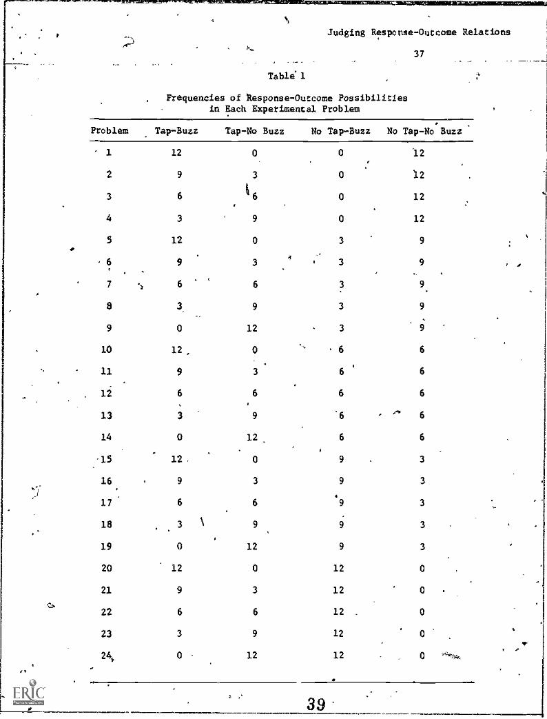
1 For each of the 24 problems, Table show the numbers of sampling inter-

vale of each of four possible types: tap-buzz,hap-no buzz, no tap-buzz, and

no tap-no bttzz. Note that the number of sampling intervals with a tap is t

equal to 12, which is the same as the number of sampling intervals without a

tap. Note also that the total number of sampling intervals equals 24. And

note finally. that the number of samplintintervaim with a buzz varies:from 3

to 24: .

\ Insert Table 1 about here

6

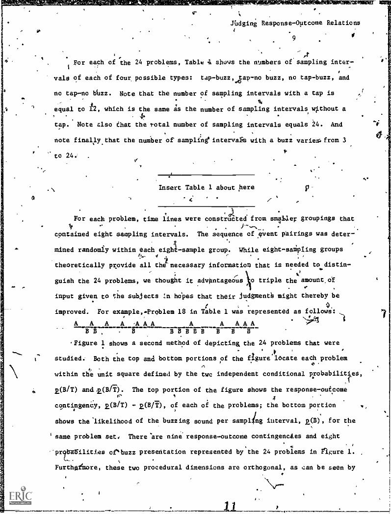
4).For each problem, time lines were constructedfrom smfllep groupings that

contained eight sampling intervals. The sequence of Avent pairings was deter-

. mined randomly within each eighl-sample group. While eight-sanipIing groups4.

theoretically provide all the7necessary information that is needed to.distin-

guish the 24 problems, we thought it advantageous o triple the amount.or

input given to t,lie subjects In hdpes that their Judgmenth might thereby be

. 0improved. For example,4roblem 18 in Table 1 was represented as follows:

AAAA,AAA A AAAAB B -------B B B B B --I B -I--

dFigure 1 shows a second method of depicting. the 24 problems that were

t studied: Both the top and bottom portions of the figure locate each problemA r.

within the unit square defined by the twc independent conditional probabilities,

2(B /T) and .2,(B /Y). The top portion of the figure Shows the response -- outcome

contingeny, 20/T) -2.(B/Y), of each of the problems; the bottom portion

shows the'likelihood of the buzzing sound per sampling interval, 00', for the

same problem set. There"Are nine response-outcome contingencies and eight

pr 6ilitles of`buzz presentation represented by the 24 problems in VIgure 1.

FurthafMore, these two procedural dimensions are orthogonal, as can be seen by

I

0

1

V

ithe 0 mite slopes of the lines that connect the 24,problems in the top and

bot m portions of the figure. From the figure it can finally be seen that

tone possible problem was not included in the set. When 2.(5/T) sa 0 im 20/i),

108) .3 0; little sense could this have been made of the task by the subjects

(see next section for questionnaire instructions).


10

Insert Figure 1 about here

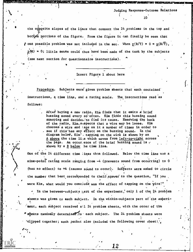
Procedure. Subjects were'given problem sheets that each contained'

instructions, a time line, and a rating scale. The instructions read as

follows:

. After buying a new radio, KiM finds that it emits g briefbuzzing sound every sd'often. Kim finds this buzzing soundannoying and decides/to find its cause. Rtmdving the backof the radio, Kim.suspects that a wire may be loose. Kimchooses a wire and taps on it a number of times in order tosee if this'has any Meet on the buzzing sound. In thediagram below), Kim'. tapping on the wire is shown by anA above the time li :.e which moves from left-to-right acrossthe page. An occur. ence of the brief buzzing sound isshown by a B below he time line.

One of the 24 different time lines then followed. Below the time line was a

nine-poin? rating scale ranging from -4 (prevents sound from occurring) to 0

(has no effect) to +4 (causes souttd to occur). Sub'j'ects were asked to circle

.

the number that best correhponded to theit\answel to the question, "If you ,

were Kim, what would you conclude, was the effect of tapping on the ire?"

In the between-subjects hart of the experiment,' only 1 of the, 24 probleM

sheets was given to each subject. In the within-subjects part of the extoeri-

k., . '4 . .,

'meat, each subject received a:1 24 problem sheets, with the order of the

*spats rendoily determindeco- each subject. The 24 problem sheets were::

'clipped together; each packet also included the following cover sheet::

e ..,14 r N

i,s ... )

32

-16

isJudging Response-Outcome Relations

11

the aim of this experiment is to see how people judgethe relationship between their actions and the consequencesof those. actions. In the 24 sheets that follow, the samebasic problem is posed: Whet is the relation between Kim'stapping on the wire of a malfunctioning radio and theoccurrence of a brief buzzing sound that the radio,pccasionallyemits. The 24 sheets differ only to the particular relationshipbetween Kim's tapping and the occurrence of the sound. Foreach of the 24 sheets, please rate the degree to which Kim'stapping affects the rate of the radio's buzzing, from "preventsthe sound from occurring" to "causes the sound, to occur." As

you go through the 24 problems, you'll soon see that the problemsdiffer from one another to varying degrees. You may sometimeswant to look back to prior problems; you may even want to changeprior responses. This is OK. It is more important to work

NLthrough the'Oroblems carefully and methodically than to givequick and offhand reactions. Indeed, the materials are paper-clipped together so that you can sort through the many sheetsand organize them any way you wish

Results'

Table 2 shows thmeans and standard deviations of subjects' judgments

for the 24 problems in both the between- and within-subjects parts of the4. .

experiment.. Each of t e 24 problems is located in the table by the coor-

dinates 2(B /T) - 2(B /F) and £(B). In general, subjects' rating scores were

positive functions ofibothe2(8 /T) - 2(B /T) and (B).

In ;ert Table 2 about here

5

Figure 2 graphically por rays subjects' rating scores as separate func-

tions Of 2(B /T). (B /T) and ...(1) in each part of the experiment. Analysis of

IPvariance simultaneously assts ed the reliability of these two sets of functions.

1

Ins.rt Figure 2 about here

The left panel of Figure 2 displays subjects' ratings as a function of

2(B /T) - 2(B /f). The F sitiv, diagonal in the figure shOws the responses of a

13

v


12

hypothetical judge whose responses correspond in a linear fashion to the

actual response-outcome contingencies and to also employs the full rating

scale. In the between- and within-subjects parts of the experiment, subjects'

judgments'Pere reliable linear functions of 2(B /T) - )F(1, 528) =

139.17, 24 .001, and F(1, 24) = 74.76, R;< .001, respectively; however, the

slopes of those functions were clearly less than that of our.hypothetical

linear observer. The between- and within-subjects functions also had reliable

quadratic components, F(1, 528) = 11.28, 2.= .001, and F(1, 24) = 28.07,

.24 .001, respectively; this trend appears to be due to the negative segments

of the functipns having shallower slopes than the positive segients. Finally,

in the within-subjects part co. the experiment, the contingency-rating function

had a reliable cubic component, F(1, 24) = 10.96, p = .003; this trend appiars

to be due to the function having an inverted S shape. Although the overall

form of the between-subjects function was similar, it did not have a reliable

cubi- component.

The right panel of Figure 2 displays subjects' ratings as a function of

2.(B). In the within- subjects part of the experiment, ratings were a positive

linear function of £(B), F(l, 24) = 32.63, 24 .001. In the between-subjects

part of the experiment, the linear trend only approached significance, F(1,

528) = 2.90, 2... .089.

To assess the relative contributions of 2.(B/T) 2,(B/T) and £(B) to sub-

jects' judgment,$) cores, the percentage of problem variance accounted for by

these factors was determined through the cubic component Rf each; beyond the

cubic component, no significant variance remained fo'V%r either part of the

experiment. In the between-subjects part of the experiment, 2(B /T) - p,(B /T),,

accounted for 86.47% of the total variance and 2.(B) accounted for 3.21%; in

the within-subjects part of the experiment, the corresponding scores were

71.87% and 24.10%.

0 14


13

Discuss3.on

Subjects' judgmentspf contingencies in the time line format showed

several interesting trends that were generally comparable in the within- and

between-subjects parts of the experiment. These results also accord well with

past paradigms using different presentation formats. First, judgments of

response-outcome correlation were a refiable,function of the r...ntingency

between the tapping of a wire and the occurr4nce of a brief buzzing sound.

1

Subjects' ratings rose as the tap-buzz contingency, 11(B/T) - 00), increased

lifrom negative to positive values. Thus, sub ects clearly showed_some sophis-

tication about apprctpriate bases of continvincy judgment.

tThe relative accuracy of subjects' jud ments is, however another issue.

Mean judgments indicated that subjects rated noncontingent relationships close

*.-to zero, but ratings of several negative elationships hovered close to zero

as well. While subject? 'ere asked to r to both the degree and thesign of a

correlation, the clearest evidence of a uracy here was the rated direction of

Zthe reljionship. Subjects' judgments huuld also have been ordered according

to'the strength of the correlation. ile this was generally true, the ratings

yielded contingency judgments that were poorer than ideal. Indeed, the quad-

/ratic component of the judgment function indicates that subjects did not treat

positive and negative relationships symmetrically; contingencies of the same

absolute value were rated as stronger for positive than for negative reia-

tiorAips. The form of this difference in ratings of relationship strength

closely resembles that found -n prior research by Erlick and Mills (1967).

The second main finding uas that judgments of correlation were reliably

influenced by the likelihood of the buzzing sound, 2(B). This bias is com-

parable to that found in other studies in which the judgment of contingency

depended on the likelihood th.tt theAutcome occurred (Allan & Jenkins, 1980;

Judginp, Resppsilse-Outcome Relations

14.

Alloy & Abramson, 1979; Jenkins & Ward, 1965). these prior studies most con-

vincingly demonstrated a bias effect of R(S) with response-outcome contin-

gencies of zero; Allan and Jenkins' (1980) investigation further suggested

that the bias effect could ;rise under positive contingencies. The present

report confirms the above trends and also shows that the effect of 2.(8) on

judgments holds under negative response-outcome contingencies as well (see

that ratings tend to increase from top to bottom within most columns of Table

2).

Experiment 2

The results of the time line portrayals in _Aperiment 1 were comparable

in many ways to those of past paradigms. However, subjects who view informa-

tion in a particular format may treat the information in a manner specific to

that format; tbs.: is, subjects' attention to information may depend on the way

the information is presented. The organization or integration of attended

information may vary with stimulus format as well. We propose three ways in

which the time line and the more familiar summary tabie'format may produce

different judgments.

l'irst, tabled prisentatIon of event frequency information offers the

subjects tallies of the frequencies of each type of event-state combination.

Our time line presentation (like past Serial presentation techniques) requires

the subjects to generate such tallies on their own. Subjects 'liven time line:

information may guess rather than count those freqUencies, resulting in esti-j

nation errors. This logic suggests that judgments with time line presentation

will be generally less accurate than judgments with tabled presentation and

that such differential accuracy will be relatively constant across positivek

negative, and noncontingent relationships. The resultant judgment function'

should be relatively flat across all contingencies compared to that of tabled

.4

iniormatAon.

16

i

NJudging Response-Outcome Relations

15

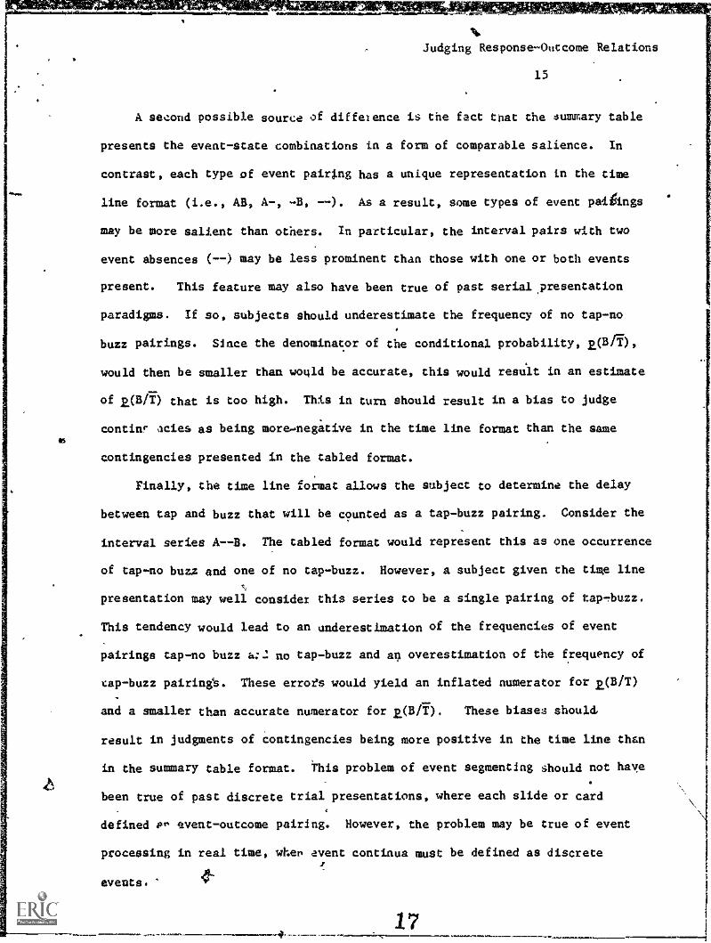
A second possible source of difference is the fact that the summary table

presents the event-state combinations in a form of comparable salience. In

contrast, each type of event pairing has a unique representation in the time

line format (i.e., AB, A-, -B, --). As a result, some types of event paigings

may be more salient than others. In particular, the interval pairs with two

event absences (--) may be Less prominent than those with one or both events

present. This feature may also have been true of past serial, presentation

paradigms. If so, subjects should underestimate the frequency of no tap-no

buzz pairings. Since the denominator of the conditional probability, .20/Y),

would then be smaller than would be accurate, this would result in an estimate

of E01/T} that is too high. This in turn should result in a bias to judge

continr acies as being more.-negative in the time line format than the same

contingencies presented in the tabled format.

Finally, the time line format allows the subject to determine the delay

between tap and buzz that will be counted as a tap-buzz pairing. Consider the

interval series A - -B. The tabled format would represent this as one occurrence

of tap-no buzz and one of no tap-buzz. However, a subject given the time line

presentation may well consider this series to be a single pairing of tap -buzz.

This tendency would lead to an underestimation of the frequencies of event

pairings tap-no buzz a:1 no tap-buzz and an overestimation of the frequency of

cap-buzz pairing's. These error's would yield an inflated numerator for E.(B/T)

and a smaller than accurate numerator for ppi/i5. These biases should.

result in judgments of contingencies being more positive in the time line than

in the summary table format. This problem of event segmenting should not haye

been true of past discrete trial presentations, where each slide or card

defined or. event-outcome pairing. However, the problem may be true of event

processing in real time when event continua must be defined as discrete

events. 4t-

rJudging Response-Outcome Relations

16

Thus, each of three reasons for judgment differences in the two informa-

tion presentation conditions would result in a unique pattern of judgment

outcomes. Whether any of these differences will materialize is an empirical

question. Experiment 2 addressed this issue by comparing judgments under the

time line format employed in Experiment 1 with judgments of the same problems4,

presented in the summary table format used in past investigations (e.g.,

Smedslund, 1963; Ward & Jenkins, 1965). Since judgments were so comparable in

the between -- and within-subjects parts of Experiment 1, subjects in Experiment

2 judged all 24 problems.

Method

Subjects. The subjects were 34 undergraduate research participants.

Problems. The same 24 problems were used here as in Experiment 1.

Problems in the time line format were typed on a single sheet of paper with

the nine-point rating scale to the right of each problem. Problems in the

summary table format were typed on-another she of paper similar to Table 1,

except that the four types of sampling intervals were vertically arrayed;

identical rating scales were located beneath each problem. Problems were

presented in a single random sequence for the time line format and'in a

different random sequence for the table format.

Procedure. During the first portion of the experimental session, sub-

jects were given an instruction sheet describing the troubleshooting problems

on the attached sheet of paper. For half of the subjects the problems were in

format, and for the other half the problems were in the summarythe time line

table format.

iu the format

lems were the

During the second half of the session, subjects worked problems

not worked in the first half. Instructions for time line prob-

same as those used in Experiment 1. Instructions for summary

table problems were the same, with appropriate adjustments to introduce the

table rather than the time line format.

18


17

Results

Table 3 shows the means and standard deviations of subject; judgments

for the 24 problems given in the time line and summary table formats. Because

analysis of variance failed to disclose any reliable effects attributable to

the order of format presentation, this factor is not considered in Table 3 nor

in later data analpsis. As in Experiment 1, subjects' ratings were positive

functiOs of both 2(B /T) - 2(B /Y) and 2(B).

Insert Table 3 about herc.,

Figure 3 graphically depicts subjects' rating scores as separate func-

tions of 2(B /T) 2(B/i7) and 2(B) for each method of information presentation:

Analysis of variance simultaneously compared these two sets of functions.


The left panel of Figure 3 portrays subjects' ratings as a function of

2(B /T) - 2(B /i). Overall,* ratings were reliable linear, F(1, 31) = 51.72,

p < .001, and quadratic, F(I, 32) = 12.90, p .. .001, functions of tap-buzz

contingency. Additionally,;there was a reliable quadratic contingency by

format interaction, F(1, 32)\= 4.97, 2 = .033. To pinpoint the source of this

3

interaction, separate analyse of variance were conducted on the time line and

summary table data. For both the time line and the summary table formats,A

ratings were reliable linear functions of contingency, F(l, 33) = 36.77,

p < .001, and F(1, 33) = 44.27, 2< .001, respectively. However, the quad-

ratic trend was reliable for the time line format only, F(1, 33) = 14.59, 2 w

.001. Thus, subjeccs' judgments were reliable linear fun(rions of response-

Judging Response-Out,:ome dulations

18

outcome contingency with both methods of information presentation; however,

the method of information presentation influenced those functions, with the

tabled format supporting judgments that better approximated those of an ideal

observer, particularly in the region of negative contingencies.

The right 2ariel of Figure 3 illustrates subjects' ratings as a function

of 2(B). Overall, ratings were reliable linear, F(1, 32) = 30.11, 2 < .001,

and quadratic, F(1, :32) = 26.68, 2.< .001, functions of outcome probability.

Additionally, there were reliable linear, F(I, 12) = 6.32, 2. = .017, and

quadratic, F(1, 32) = 12.94, 2 < .001, outcome prohbility by format inter-

S

actions. Because of these interactions, follow-up analyses were separately

1

performed on the time line and summary table data. For the time line data,

ratings were reliable linear, F(l, 33) = 34.37, 2.< .001, and quadratic, F(1,

33) = 30.43;2. < .001, functions of 2SB); for the summary table data, the

linear trend was reliable, F(1, 33) = 5.33, 2.= .027, and the quadratic trend

fell just short of statistical significance, F(l, 33) = 3.69, P = .063. Thus,

the method of information pre ntation altered the.influence of outcome proba-

bility on subjects' ratings; providing the information in a time line format

both steepened the probability-judgment function and increased its curvature

relative to providing the same information in a summary table format.

And, regardless of tap-buzz contingency and buzz probability, judgments

were reliably higher in the time line condition, than in the slmary table

condition, F(1, 32) = 5.03, 2 = .032.

TO assess the relative contributions of response-outcome contingency and

outcome probability to subjects' ratings, the percentage of problem variance

accounted for by each factor was determined as in Experiment 1. For the

summary table data, 2(B/T) - 2(E/F) accounted for 81.35% of die total variance

and 2(B) accounted for 12.58%; for the time line data, the corresponding

go

Judging Response-04tcome Relations

19

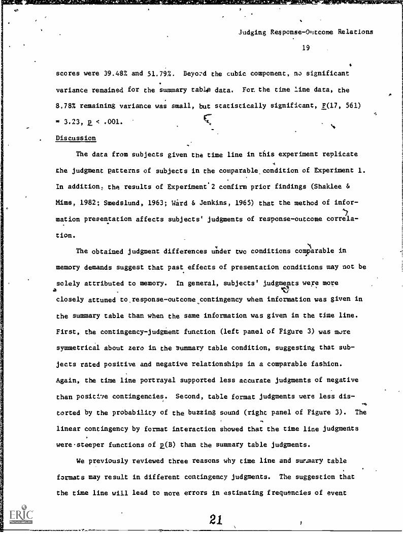
scores were 39.48% and 51.79%. Beyo:d the cubic component, no significant

variance remained for the summary table data. For, the time line data, the

8.78% remaining variance was small, but statistically significant, F(17, 561)

im 3.23, k < .001.

Discussion

The data from subjects given the time line in this experiment replicateA

the judgment patterns of subjects in the comparable condition of Experiment 1.

In addition; the results of Experiment.2 confirm prior findings (Shaklee &

Mims, 1982; Smedslund, 1963; Wird & Jenkins, 1965) that the method of infor-

'7or presentation affects subjects' judgments of response-outcome correla-

tion.

Tice obtained judgment differences under two conditions comparable in

memory demands suggest that past effects of presentation conditions may not be

solely attributed to memory. In general, subjects' iudgmepts were morea

closely attuned to.response-outcome contingency when information was given in

the summary table than when the same information was given in the time line.

First, the contingency-judgient function (left panel of Figure 3) was mare

symmetrical about zero in the Summary table condition, suggesting that sub-

jects rated positive and negative relationships in a comparable fashion.

Again, the time line portrayal supported less accurate judgments of negative

than positie contingencies. Second, table format judgments were less dis-

torted by the probability of the buzzing sound (right panel of Figure 3). The

linear contingency by format interaction showed that the time line judgments

were steeper functions of £(B) than the summary table judgments.

We previously reviewed three reasons why time line and summary table

formats may result in different contingency judgments. The suggestion that

the time line will lead to more errors in estimating frequencies of event


20

(

pairings than the summary table predicted overall poorer contingency judgment

Accuracy (i.e., a flatter, but symmetrical contingency-judgment function) in

the time line than in the tabled format condition. The possibility that joint

event ab ?ences (no tap-no buzz) were less salient in the time line than in the

tabled presentation' mode predicted a general bias to report relationships as

more negative in the time line than in the summary table format. However,

neither of these' difference patterns describe our results.

Subjects in this experiment did show a tendency to judge relationshipi as

more positive in the time line than in the summary table condition. This c

result supports our third proposed source of differences, that subjects may

1,7"- group event pairings differently in the time line than the tabled format. In

particular, event Levies A -B could be identified as a single tap-buzz occurrence

rather than a tap-no buzz-and a no tap-buzz, yieldirg in a bias to report

relationships as positive. However, we should note that while ratings were

generally higher in the time line than in the summary table condition, the

positivity bias was more pronounced for negative than positive contingencies.

One possible account for this finding involves the influence of context on the

grouping of event pairings; that is, A--B may be most likely to be judged a

tap-buzz occurrence when there are few contiguous AB pairings in the time

line, as would be the case in negative contingencies.

Besides helping us to understand why different presentation formats sup-er

port different judgments, these performance differences between groups also

allow us to.reject the possibility that time line subjects' problems with

rating negative contingencies are due to a response bias or to prior expecta-

tions. Any expectation about the effect of tapping on the radio's buzzing

should be the same in the two groups, but judgments of negative contingencies

were distorted feriime line subjects only. Similarly, since subjects made

22

444


21

judgments on the same rating scale in the two conditions, gerforMance dif-

ferences cannot be attributed to peculiarities in the scale itself.

4Experiment 3

The results thus far suggest that subjects may define events differently4 V

in the time line and table forMats. If this is the principal reason for the

inaccurate responses of time line subjects, theh their judgments should

improve when the continuous stream of events in the time line.is separated

into discrete units.

Our third experiment further explored'the problem of defining individual

sampling periods by placing a clear break between paired.intervals in the time

line forpat. To do this, we simply, added a blank space between successive

sampling intervals along the time line. As in the within-subjects part of

Experiment 1, subjects rated all 24 tap-buzz contingencies. These 'judgments

were compared to those obtained in Experiment 1,. in which successive sampling

intervals immediately followed one another:

Method

Subjects. Another group of 25 undergraduate research participants joined

the 25 vlbo had served in the within-subjects part of Experiment 1, and whose

data are depicted again-in the Results section that follows. Subjects in

these two groups vere from the same introductory psychology course and were

tested within 3 weeks of the same school term.

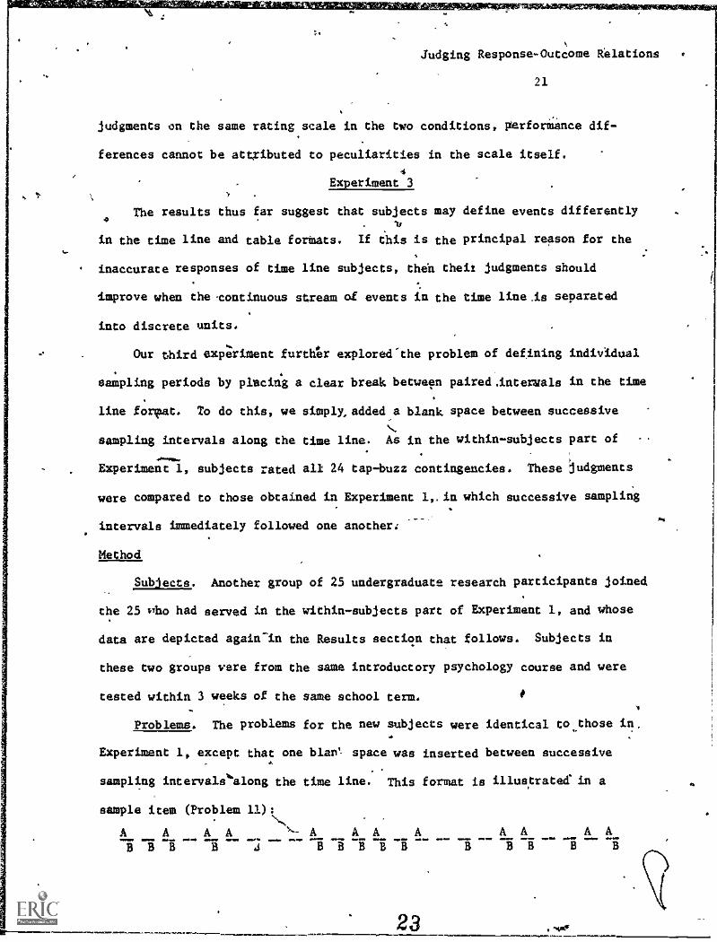
Problems. The problems for the new subjects were identical tothose in.

Experiment 1, except that one blaW- space was inserted between successive

sampling intervale'along the time line. This format is illustrated in a

sample item (Problem 11)AAAA \-AAAA AA AA1 I -I i -I -I E -I I -I B I I

23


, 22

Procedure. The procedure for the new subjects given the broken time

lines was identical to that'for the former subjects given the unbroken tie

lines in,Experiment 1.

'Results

Table 4 shows the means and standard deviations of subjects' -judgments

for the 24 probldms given in the broken and the unbroken time line conditions

of Experiment 3. ,Again, subjects' ratings were positive functions of 2(B /T) -.

20/i5 a'1id.2(8).

Insert,Table 4 about here

Figure 4 graphically illustrates subjects' rating scores as separate

functions of 2(B /T) - 2(8 /i) and 2(B) for each time line-condition. Analysis

of variance simultaneously compared these two sets of functions.


The left panel of Figure 4 shows, subjects' ratings as a function of

i(B/T) 2(B /i). Overall, ratings were reliable linear, F(1, 576) 0.542.75,,

E 2 .001, quadratic, V1, 570) 34.32, 2 < .001, and cubic, P(I, 576/

20.35, 2 < .001, functions of tap-buzz contingency. Additionally, there was a

.reliable linear contingency, by time line interaction, P(1, k76) = 5.08, 2

.025, and a near significant quadratic contingency by time line interaction;

F(1, 576) 3.18, 2. :075. Therefore, separate analyses of variance were

-conducted on the data for the group given the broken time line and for the

group given the unbroken time line. Air both the broken and unbroken time

lime groups, ratings were reliable linear functions, P(1, 24) 83.74, 2 < .001,

24.01.

Judging Response Outcome Relations

23

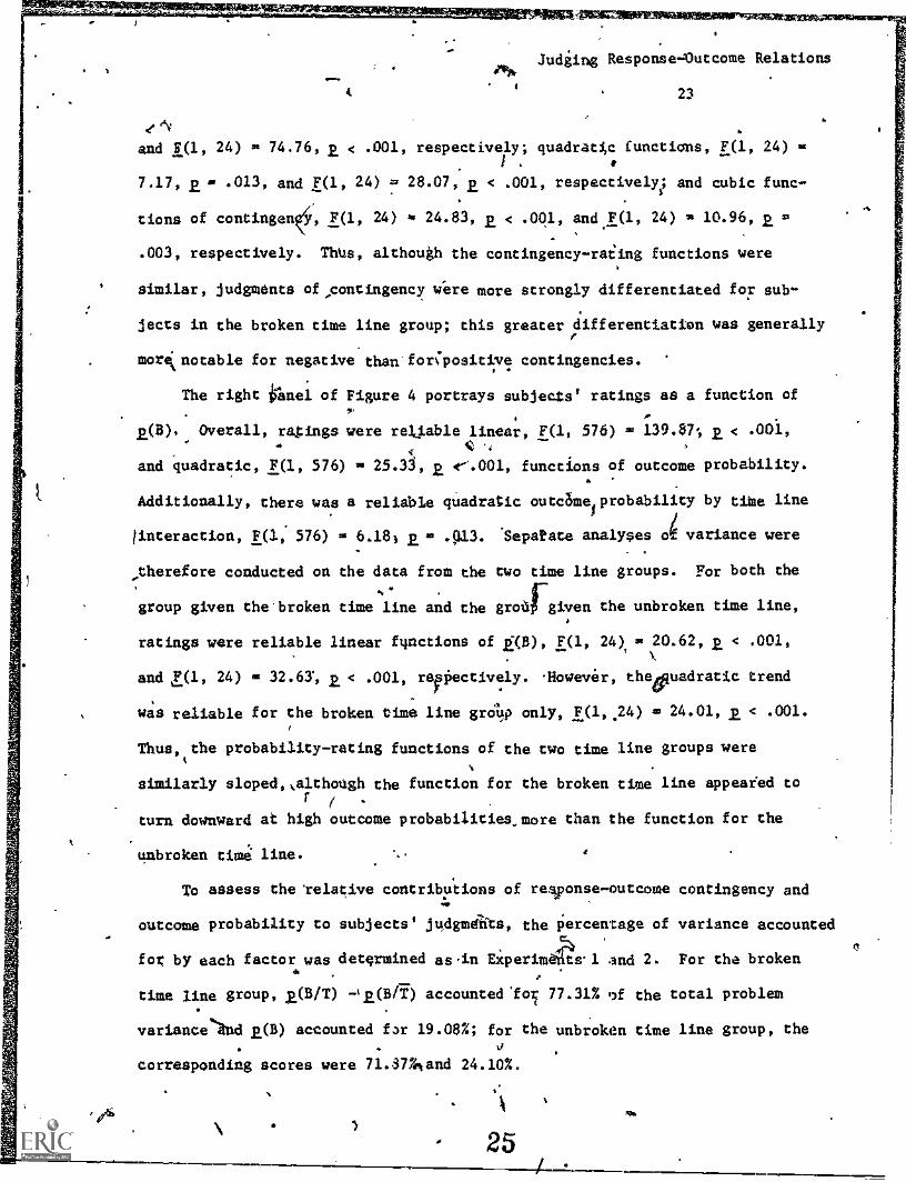
and 1(1, 24) = 74.76, P < .001, respectively; quadratic functions, F(1, 24) =

7.17, 2, = .013, and F(1, 24) = 28.07, k < .001, respectively; and cubic func-.

tions of contingent, F(1, 24) it, 24.83, k < .001, and.F(1, 24) = 10.96, P =

.003, respectively. ThUs, although the contingencyrating functions were

similar, judgments of,contingency were more strongly differentiated for sub-

jects in the broken time line group; this greater differentiation was generally

more otable for negative than'foripositive contingencies.

The right iranel of Figure 4 portrays subjects' ratings as a function of

2.(8). Overall, ratings were reliable linear, F(1, 576) = 139.87.; < .001,

and quadratic, F(1, 576) = 25.33, P 4--.001, functions of outcome probability.

Additionally, there was a reliable quadratic outanelprobability by time line

!interaction, F(1; 576) = 6.18; 2Las .913. 'Separate analyses o4 variance were

therefore conducted on the data from the two time line groups. For both the

group given the'broken time line and the groaf-given the unbroken time line,4,

ratings were reliable linear Ainctions of 2(B), F(1, 24), = 20.62, < .001,

and B1, 24) = < .001, respectively. iowever, theivadratic trend

was reliable for the broken time line grO4p only, F(1,,24) = 24.01, jl< .001.

'Thus, the probability-rating functions of the two time line groups were

similarly sloped"although the function for the broken time line appeared toF /

turn downward at high outcome probabilities more than the function for the

unbroken time line.

To assess the 'relative contributions of response-outcome contingency and

outcome probability to subjects' judgmats, the Percentage of variance accounted

fox by each factor was determined as.in ExperimeaS.1 and 2. For the broken6

time line group, 20/T) -42.(11/Y) accounted 1o5 77.31% of the total problem

varianceInd 2(B) accounted far 19.08%; for the unbroken time line group, the

corresponding scores were 71.$7ZNand 24.10%.

25

Discussion ay.

.

) . '"

Judging Response-Ouccome.Ralitions

24

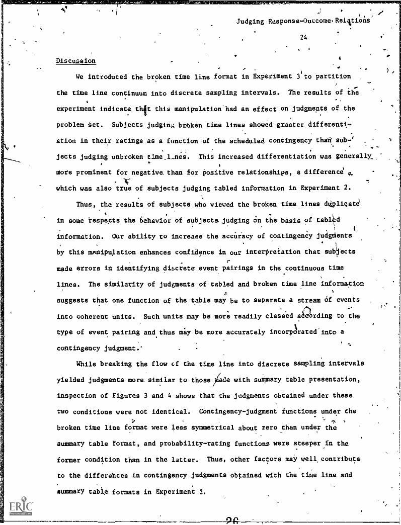
We introduced the broken time line format in Experiment 3'to partition

.

the time line continuum into discrete sampling intervals. The results of the

experiment indicate thit this manipulation had an effect on judgments of the

problem set. Subjects judging broken time lines showed greater differenti-

ation in their ratings as a function of the scheduled contingency theft sub-'

jecte judging unbroken time.1-nes. This increased differentiation was generally .'%

more prominent for negative than for positive relationships, a difference 4,

truewhich was also true of subjects judging tabled information in Experiment 2.

Thus, the results of subjects who viewed the broken time lines diplicate

.

in some respects the behavior of subjects judging on the basis of tabildt

information. Our ability to increase the accuracy of contingency judgdenes

by this mAnipulation enhances confidence in our interpretation that subjects

made errors in identifying discrete event pairings in the continuous time

lines. The similarity of judgments of tabled and broken time line information

4

suggests that one function of the table may be to separate a stream of events

into Coherent units. Such units may be more readily claSsed aiarding to the

type of event pairing and, thus may be more accurately incorOreted'into a

contingency judgment.'

While breaking the flow of the time line into discrete sampling intervals

yielded judgments more similar to those ,iade with summary table presentation,

inspection of Figures 3 and 4 shows that the judgments obtained under these

two conditions were not identical. Contingency - judgment functions under the

broken time line format were less symmetrical about zero than under the

summary table format, and probability-rating functions were steeper in the

former condition than in the latter. Thus, other factors may well. contribute

to the differehtes in contingency judgments obtained with the time line and

summary table formats in Experiment 2.


25

Experiment 4

Thus far, our leading interpretation of the problems created by-a con-

tinuous representation of events is that people have difficul v breaking the

stream into discrete units. An alternative approach to testing this account

might be to teach people to parse the time line into the component units. If

such training produes judgment functions like those found in our broken time

line and table formats, such findings would further support this as the source

of judgment differences. A second innciion of the table mentioned earlier0,

might be to offer subjects numerical summaries of the information about the

four event combinations. This summarized information may be more readily

incorporated Ant° a decision rule in judging event covariations. In this way,

judgment accuracy might be further enhanced if subjects were asked to count

the occurrences of each event-state combination and note these frequencies

in a table. By this process, subjects would effectively convert a time line

into a table format.

Our fourth and final experiment used each of these approaches. One group

of subjects was presented with the 24 problems in our original time line

format, but were taught to break the line into response-outcome intervals

(line-interval). A second group received these instructions and were also

asked to count the frequencies of each event-state pairing and write those

frequencies in a tale (line-table). Time line and table groups using our

original instructions served az comparison conditions for these manipulations.

impreved judgment by line-interval subjects.comparri to time line subjects

-would further implicate line segmenting as a factor in contingency judgment.

Further improvesdEts by line-table subjects would suggest that summary infor-

mation is also an important function of the tahled format. Because we found

sex differences in contingency judgment in related work of ours (Shaklee &

Hall, in press), sex was included as a factor in this experiment.

27


26

Method

Subjects. A total of 160 introductory psycholOgy subjects served in the

experiment with 20 males and 20 females.in each of four judgment conditions.

Problems. The 24 contingencies for this experiment were the same asS''

those in the previous expeiiments. Format of problems in the time line and

table representations was the same 4s that used in Experiments 1 and,2.

Procedure. The' introduction to the troubleshooting problems was identi-

cal ri that used in the previous studies, except that the problem representa-

tion was explained in one of four ways:

Line: These instructions were the same as those used in Experiments 1

and 2.

Line-Interval: The problems were represented in a time line like that

used in Experments I ad 2, but in this case subjects were specifically

instructed how to break the time line into response-outcome intervals. In-

structions were as follows:

Each dash on the time line represents one unit of time.Time units come in pairs, with the first an opportunityfor a response (Tap or No Tap) and the second an opportunityfor an outcome (Buzz or No Buzz). Thus, pairs of successiveintervals can be of four types: Tap-Buzz, Tap-No Buzz, NoTap-Buzz, No Tap-No Buzz. For each of the time lines, pleaserate the degree to which Kim's tapping affects the rate ofthe radio's buzzing, from "prevents the sound from occurring"to "causes the sound to occur."

Line-Table: Problems and instructions were identical to-those in the

Line-Interval condition, except that, each problem was accompanied by a bliank

table labeled as in the previous table condition of Experiment 2. SubjeCts

were instructed to complete the table before making their judgment. Instruc-

0tions were as follows:

4

Each dash on the time line represents, one unit of time.Time units coMe,in pairs, with the first an opportunity fora response (Tap or No Tap).and the second an opportianity for

28


27

(a outcome (fuzz or No Buzz). Thus, pairs of successiveintervals can be of folv types: Tap-Buzz, Tap-No Buzz, NoTap-Buzz, No Tap-No Buzk. For each time line, please countthe frequency of each of these four types of interval pairs.Enter those frequencies in the table to chi right of the timeline. Once you have completed the table, please rate thedegree to whick Kim's tapping affects the rate of the radio'sbuzzing, from "prevents the sound from occurring" to "causesthe sound to occur."

Table: Problems and instructions in this condition were identical to

those is Experiment 2.

I each condition, the information offered in the instructions Js shown

on a sample problem illustrating each type of response-outcome pairing.

Subjects were invited to ask any questions they might have, after which they

proceeded at their own pace through the problem set.

Results

Means and standard deviations of subjects' judgments for the 24 problems

in each judgment condition ace shown in Table 5. Figure 5 illustrates sub-

jects' judgments of the nine contingencies, 20/T) - 2.(E/f), and the eight

probabilities of buzzing sound, gat), for the four judgment conditions. These

functions were simultaneourly compared by analysis of variance, including sex

of subject and judgment condition as factors. Paired follow-up analyses were

aonducted on interactions, setting alpha at .025 to reduce the experiment-wide

error rate.

Insert Table 5 and Figure 5 about here

The overall analysis yielded reliable linear, F(1, 152) 851.86, lt< .001,

quadratic F(1, 152) mg 100.92, p < .001, and cubic F(1, 152) S. 12.52, B. < .001

trends of response-outceme contingency on subjects' judgments. As it our

previoUs experiments, judgments were a function of problem contingency, but

4)k 29 .

10'

Judging Response-Outnome Relations

28

with judgments of negative relations closer to zero than those of posaive

relations. This analysis also showed a main effect of judgment condition,

F(3, 152) = 11.40, P < .001, although that effect is qualified by a contin-

gency by condition interaction, F(23, 306) = 2.47, 2. < .001. As seen in the

left portion of Figure 5, the form of this interaction shows that Judgments in

the Table condition were most symmetrical about zero, Judgments in the Line

condition were least symmetrical, and judgments in the Line-Interval ano Line-

able conditions fell between these two extremes. Follow-up analyses.compared

contingency jungment functions for selected condition pairs. Line-interval

and Line conditions were compared to identify the effect of the interval

segmenting instructions. This analysis showed Line - Interval subjects to be

significantly different from Line subjects; linear trend F(1, 76) = 11.12, 2L=

.001, the quadratic trend approaching significance f(l, 76) 40 4.92, .R. = .029.

Comparison of Line-Table and Line-Interval contingency functions showed that

tabling the frequency information had no additional effect on judgment accuracy.

Line-Tableand Table j'ges were compared co see if judges who tabled the

frequency information for themselves were equivalent in Judgment to those who

judged tables provided by the experimenter. This comparison showed that

contingency judgment fUnctions were not equivalent for the two groups, with

Line-Table and Table judges reliably different in quadratic trend, F(1, 76) =

5.83, 2. ='.018, but not in linear or cubic trends.

Sex differences in contingency functions were statistically significant,

with the contingency-judgment function for females flatter than that, for

males: linear trend F(1, 152) = 3.94, .049, cubic trend F(1, 152) = 4.38,

2, .0 .038. This aex effect did not interact significantly with judgment condition.

As in our previous experiments, subjects' judgments were an increasing

function of the probability of the buzzing sound (see right portion of Figure

it


29

5). Ratings showed significant linear, F(1, 152) m= 210.66, z< .001, quad-

ratic, F(1, 152) 80.90, z< .001, and cubic, F(1, 152) mi 4.58, 2, .034,

trends as a function 'of 03). Unlike previous analyses, however, these

probability-judgment functions were not reliably affected by judgment condi-

tion, although the Line group again showed the greatest effect of 00 and the

Table group showed the least effect. Effects of £(B) aim, did not differ as a

function of subjects' sex.

The relative contributions of response-outcome contingency and outcome

probability in each of the four conditions were determined as in the prior

experiments. For the Table group, 2.(B/T) - 03/76 accounted far 89.07% of the

total problem variance and 03).accounted for 9.47%; for -thq Line-Table group,

the corresponding scores were 80.97% and 17.02%; for the Line-Interval group,

the scores were 76.04% and 17.61%; and f9k the Line groap,'the scores were

71.38% and 22.64%. In only the latter two groups was the residual variance

significant: Line-Interval residual mi 6.35%, F(17, 646) 6.72, z < .001, and

Line residual at 5.98%, F(17, 646) it 2.25, 2. .003.

Since frequency judgment errors may detract from contingency judgment

accuracy, the frequency tables generated by subjects in the Line-Table condi-

tion were examined for accuracy. Overall, errors were small, with mean

absolute deviations of .15, .10, .30, and 1.65 for Tap-Buzz, Tap-No Buzz, No

Tap -Buzz, and No Tap-No Buzz frequencies, respectively. In view of the dif-

ferential judgments of positive and negative relationships in this condition,

'frequency judgment accuracy was compared for problems representing positive

and negative contingencies. Absolute deviations were averaged across table

cells for this analysis. A matched-pairs t --test showed no reliable differences

in frequency judgment errors on positive and negative contingencies, t(39) < 1.

Discussion

aperiment 4 represents a conceptual replication of our third experiment.

31


30

In Experiment 3, we broke the time line into discrete units. In this experi-

ment, we taught the subjects themselves to define these intervals. The results

indicate that the manipulations in the two experiments had similar effects.

Line - Interval and Line-Table subjects in Experiment 4 produced contingency-,

judgment functions intermediate to those of our Line and Table subjects.

Line-Interval and Line-Table subjects' contingency-judgment functions were

more symmetrical about zero than that of Line subjects, although the two new

conditions did not differ from each other. This failure to find additional

improvement by subjects who completed a frequency table indicates that the

availability of summary information contributes little to judgment accuracy.

However, the similarity of these two functions to that of subjects in our past

broken time line condition enhances our confidence in the problem of event

segmenting as a source of error in judging negative relationships.

The finding that Line-Table judges are also less accurate than Table

judges is a bit of a surprise. These subjects have effectively converted time

line information into a tabled float. However, the accuracy of that conversion

is a second question. Since any deviations infrequency judgments must

necessarily be in the direction of lower accuracy, subjects in this condition

may have somewhat erroneous information on Which to base their judgments.

However, a look at subjects' frequency counts indicates reasonable accuracy;

indeed, 12 out of 40 subjects did not show a single- error on any of the 24

problems. In adaition, error rates were similar on negative and positive

.contingency problems. "Thus, inac6uracy of-frequency jitdgm6ts constitutes a

weak account of the difference is judgment functions of Line-Table and Table

subjects.

These differences between Line-Table and Table judgments replicate the

stimulue presentation effects of Ward and Jenkins (1965) in a substantiallyw,'

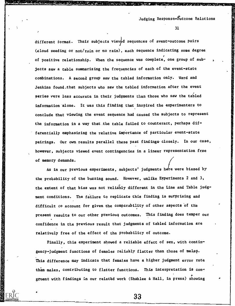
Judging Response - outcome Relations

31

different format. Their subjects view d sequences of avent-outcome pairs

(cloud seeding or not/rain or no rain), each sequence indicating some degree

of positive relationship. When the sequence was complete, one group of sub-

jects saw a table summarizing the frequencies of each of the event-state

combinations. A second group saw the tabled information only. Ward and

Jenkins found-that subjects who saw the tabled information after the event

aeries were less accurate in their judgments than those who saw the tabled

information Alone. It was this finding that inspired the experimenters to

conclude that viewing the event sequence had caused the subjects to represent

the information in a way that.the table failed to counteract, perhaps dif-

ferentially emphasizing the relative importance of particular event-state

pairings. Our own results parallel these past findings-closely. In our case,

however, subjects viewed event contingencies in a linear representation free

of memory demands.

As in our previous experiments, subjects' judgments h re were biased by

the probability of the buzzing sound. However, unlike Experiments 2 and 3,

the extent of that bias was not reliably different in the Line and Table judg-

ment conditions. The failure to replicate this finding is surprising and

difficult to account for given the comparability of other aspects 'of the

present results to our other previous outcomes. This finding does temper our

confidence in the previous result that judgments of tabled information are

relatively free of the effect of the probability of outcome.

Finally, this experiment showed a reliable effect of sex, with contin-

gency-judgment functions of females reliably flatter than those of males.

This difference may indicate that females have a higher judgment error rate

th6 males, contributing to flatter functions. This interpretation is cow,

gruent with findings in our relatbd work (Shaklee & Hall, in press) showing

33


32

that Females use simtpler, less accurate rules tiiiiShoseilia-by

judge event covariations. An alternative interpretation of the sex differences

in the present experiment is that-the two sexes judge the problems with similar

accuracy, but that the females use a more limited range of the scale to make

their judgments. However, a comparison of judgments indicates that the two

sexes use the scale extremes (+4) at comparable rates (11.3% and 12.2% of

judgments for males and females, respectively), ruling out response conser-4

vatism as a viable account of this sex difference.

Concluding

In overview, the results of four different experiments suggest that

judgments of interevent contingency importantly depend on the method of

presenting information about event pairings. Most accurate were judgments of

summary table information (Experiments 2 and 4); least accurate were judgments

of information presented in a continuous time line format (Experiments 1, 2,

and 4). The accuracy of subjects judging partitioned time lines (Experiment

3) fell in between that of the other two conditions. Eubjectsrtrained to

segment continuous time lines (Experiment 4) made judgments similar to those

who saw partitioned time lines. .This evidence suggests that Ward and Jenkins

(1965) were correct in their suspicion that presentation format may influence

subjects' treatment of frequency information in making contingency judgments.

Our evidence indicates that subjects may break event sequences into different

discrete event pairings depending on the format in which the frequency infor-

maiion is presented. Tills explanation accounts well for our own findings, ,but

may not be similarly useful in explaining the effects of relationship direction

in some past paradigms. As noted earlier, slide or card sequence presentations

offer event pairings as discrete units rasher than as event Continua.

This interpretation offers a ready account for the finding in past

research that subjects judge negative relationships less accurately' than

Judging Reponse -Outcome Relations

33

positive relationships. Past researchers have suggested qat subjects know

how to judge positive, but not negative contingencies. All (1980), however,

n5pointed out one difficulty With this interpretation; subjec s who only know

how to judge positive relationships must be able to distinguish between posi- .7'

tive and negative relationships in order to apply the appropriate rule to

4

positive contingencies. Presumably, a different, less accurate rule is

applied to negative (and independent) relationships. Thus, this interpreta-

tion requirez that an individual maintain more than one rule to judge event

contingencies, and that the person know, when to apply which rule to which

relationship.

Our analysis indicaLes a single judgment problem which would result in

differential accuracy on positive and negative relationships: that is, sub-,

jects' boundaries for event segments depend on the other events in the stream.

Positive relationships are typified by many response-outcome pairs which would

define a brief time interval as a response-outcome unit. However, where few

outcomes promptly follow responses, the observer may accept relatively delayed

outcomes as "caused" by the response. The estimate of response-outcome pairs

is inflated, resulting in an illusion of a relationship which is less negative

bean is objectively the case.

We would argue that the problems our subjects encountered in the time

line format could be similar to those encountered in judgments of real world

contingencies--response-'outcome delays may vary in everyday experience. One

task of the perceiver is then to define which sequences represent true response-

outcome pairings. Investigations of the cues used to b reak event sequences

into discrete units are rare. Our evidence suggests that understanding this

process may be important to our ability to account for contingency judgments.

35


References

34

Allan,-L. A note on measurements of continency between two binary variables.

in judgment tasks. Bulletin of the Psychonomic Society. 1980, 415, 147-149.

Allan, L., & Jenkins, H. The judgment of contingency and the nature of the

response. Canadian Journal of Psychology/Review of Canadian Psychology.,

1980, 34, 1-11.

Alloy, L., & Abramson, I. Judgment of contingency in depressed and nondepressed

students: Sadder but wiser? Journal of Experimental Psychology: General,

1979, 108, 441-485.

Chapman, L., & Chapman, J. Genesis of popular but erroneous psych diagnostic

observations. .Journal of Abnormal Psychology, 1967, 72, 193-204. (a)

Chapman, L., & Chapman, J. IlluOory correlation as an obstacle to the use of

valid psychodiagnostic signs. Journal of Abnormal Psycholly, 1967, 74,

271-280. (b)

Crocker, J. Judgment of covariation by social perceivers. Psychological

Bulletin, 1981, 90, 272-292. 1

Erlick, D. E., & Mills, R. G. Perceptual quantification of conditional depen-

dency. Journal of Experimental Psychology, 1967, 43, 9-14.

Heider, F. The psychology of interpersonal relations. New York: Wiley, 1958.

Hume, D. A treatise of human nature. In A. Flew (Ed.i, On human nature and

the understanding: New York: Collier, 1962. (A Treatise of human nature

was originally published in 1739.)

Infielder, B., & Piaget, J. The growth of logical thinking from childhood

to adolescence. New York: Basic Books, 1958.

Jenkins, H., & Ward, W. Judgment of contingency between responses and outcomes.

PsycholoOcal Monographs, 1965, 79, 1-17.

Keliey,,H. H. Attribution theory in social psychology. In D. Levine (Ed,),

Nebraaka Symposium on Motivation (vol. 15). Lincoln: University of

Habra ess, 1967.36


351

.....o..........Mackintosh, N. J. The psychology of animak learning.. London: Academic Press,

1974.;

Morgan, C. L. The limits of animal intelligence. Fortnightly Review, 1893.

54, 223 -239.

Morgan, C. L. An introduction to comparative psychology. London: Walteru

Scott, Ltd., 1894.

f/-7IRescorla, R. A. Some in-lications of a.cognitive perspective on Pavlovian

. conditioning. In S. H. Hulse, H. Fowler, & W. K. Honig (Eds.), Caektve

processes in animal behavior. Hillsdale, NJ: ErlbauM, 1978.

Seggie, 4. The empirical observation of the Piagetian concept of correlation.

Canadian Journal of Psychology/Review of Canadian Psychology, 1975, 29, ,

32-42.

Seggie, J., WEndersby, H. The empirical implications of Piaget's concept of

`correlation. Australian Journal of Psychology, 1972, 24, 3-8.

Shaklee, H., & Hall, L. Methods of assessing strategies judging covaril.

ation between events.. Journal of Educational Psychology, in press.

Shaklee, H., & Mims, M. Sources of error in judging event covariations: EffectsaGf

of memory demanda. Journal of Experimental Psychology: Learning, Memory,

and Cognition, 1982, 13, 208-224.

Shaklee, H., & Tucker, D. A rule analysis of judgments of covariation between

events. Memory and Cognition, 1980, 8, 459-467.

Smedslund, J. The concept of correlation in adults. Scandinavian Journal of

tychologx, 1963,.4, 165-173.

Ward, W., & Jenkins, H. The display of information and the judgment of contin-

gency. Canadian Journal of Psychology, 1965, 19, 231-241.

37

AoJudging Response-Outcome Relations

36

11C-80-0091 to H.S. The authors are greatly indebted to R. H. Roble for his

This research was supported by NSP grant 79-14160 to E.A.W. and NIE giant

,

%:,,

.

Footnote

li

\I

helpful technical assistance. Portions of this research were reported at the

annual meeting of the Psychonomic Society, Philadelphia, PA, November, 1981.

,

t.

Requests for reprints may be sent to either author, Department'of Psychology,

The University of Iowa, Iowa City, IA 52242.

4

38

4.

4.

A


37

Table'l

Frequencies of Response-Outcome Possibilitiesin Each Experimental Problem

Problem Tap-Buzz Tap-No Buzz No Tap-Buzz No Tap-No Buzz

' 3. 12 0 0 '12

2 9 3 0 12

3 6 6 0 12

4 3 9 0 12

5 12 0 3 9

6,

9 3 3 9

7 6 6 3 9.

8 3 9 3 9

9 0 12 3 9

10 12, 0 6 6

11 9 3 6 6

12 6 6 6 6

13 3 9 .6 6

14 0 12 6 6

-15 12 . 0

,

9 3

16 9 3 9 3

17 6 6,

9 3

18 3 9 9 3

19 0 12 9 3

20 12 0 12 0

21 9 3 12 0

22 6 6 12 0

23 3 9 12 0

244 0 12 12 0A

39

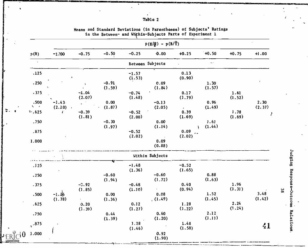
40

Table 2

Means and Standard Deviations (in Parentheses) of Subjects" Ratingsin the Between- and Wilfhin-Subjects Parts of Experiment 1

P(14) P(B/f)

P(B) -1:00 -0.75 -0.50 -0.25 0.00 +0.25 +0.50 +0.75

Between Subjects

.125 -1.57 0.13(1.53) (0.90)

.250 , -0.91 0.09 1.30(1.59) (1.84) (1.57)

.375 -1.04 -0.74 0.17 1.61(2.07) (1.48) (1.79) (1.52)

.500 -1.43 0.00 -0.13 0.96t. ,

v-.625

(2.10) .

i -0.39

(1.87) (2.05)

-0.52.

0.39(1.49)

1.78

(1.81) (2.00) (1.69) (1.69)

.750 -0.30 0.00 /.61

(1.97) (1.14) y (1.44)

.875 -0.52 0.09(2.02) (2.02)

1.000 0.09(0.88)

Within Subjects

.125 -1.48 -0.52(1.36) (1.65)

.250 -0.60 -0.60 0.88

(1.94) (1.72) (1.63)

.375 -0.48 0.40 1.96

(1.85) (1.10) (0.94) 0.31).500 0.00 0.08 1.52

(1.78) (1.36) ,(1.49) (1.45)

.625 0..20 0.12 1.28 2.24

(3.39) (1.27) (1.22) (1.24)

.750 0.44 0.60 2.12

(1.39) (1.20) (1 .11 )

.8751

1.28(1.46)

1.48

(1.58)

1.000 0.92

(1.90)

+1.00

2.30

(2.37)

,i,

os3.48 o

1.7

(1.42) o0am

41

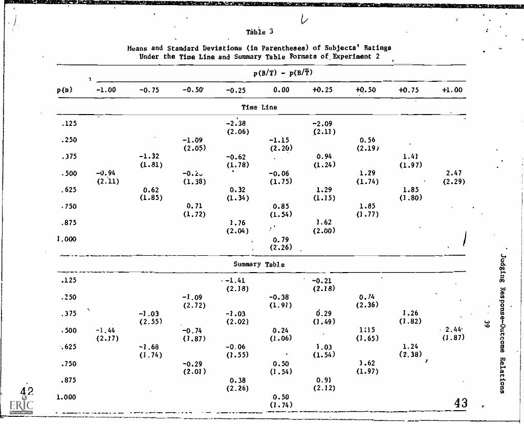
4 2

Table 3

Means and Standard Deviations (in Parentheses) of Subjects' RatingsUnder the Time Line and Summary Table Formats of,Experiment 2

p(B/T) P(B/t)

P(b) -1.00 -0.75 -0.25 0.00 +0.25 +0.50 +0.75

Time Line

.125 -2.38 -2.09(2.06) (2.11)

.250 -1.09 -1.15 0.56(2.05) (2.20) (2.19)

.375 -1.32 -0.62 0.94 1.41

(1.81) (1.78) (1.24) (1.97)

.500 -0.94 -0.... -0.06 1.29(2:11) (1.38) (1.75) (1.74)

.625 0.62 0.32 1.29 1.85(1.85) (1.34) (1.15) (1.80)

.750 0.71 0.85 1.85

(1.72) (1.54) (1.77)

.875 1.76 1.62

(2.04) (2.00)

1.000 0.79(2.26)

Summary Table

.125 -1.41 -0.21(2.18) (2.18)

.250 -1.09 -0.38 0./4

(2.72) (1.91) (2.36)

.375 ' -1.03 -1.03 d.29 1.26

(2.55) (2.02) (1.49) (1.82)

.500 -1.44 -0.74 0.24 125(2.X7) (1.87) (1.06) (1.65)

.625 -1.68 -0.06 1.03 1.24

(1.74) (1.55) (1.54) (2.38)

.750 -0.29 0.50 1.62 :

(2.01) (1.54) (1.97)

.875 0.38 0.93

(2.26) (2.12)

1.000 0.50(1.74)

+1.00

2.47

(2.29)

(...)

2.44% '0(1.87)

43 0

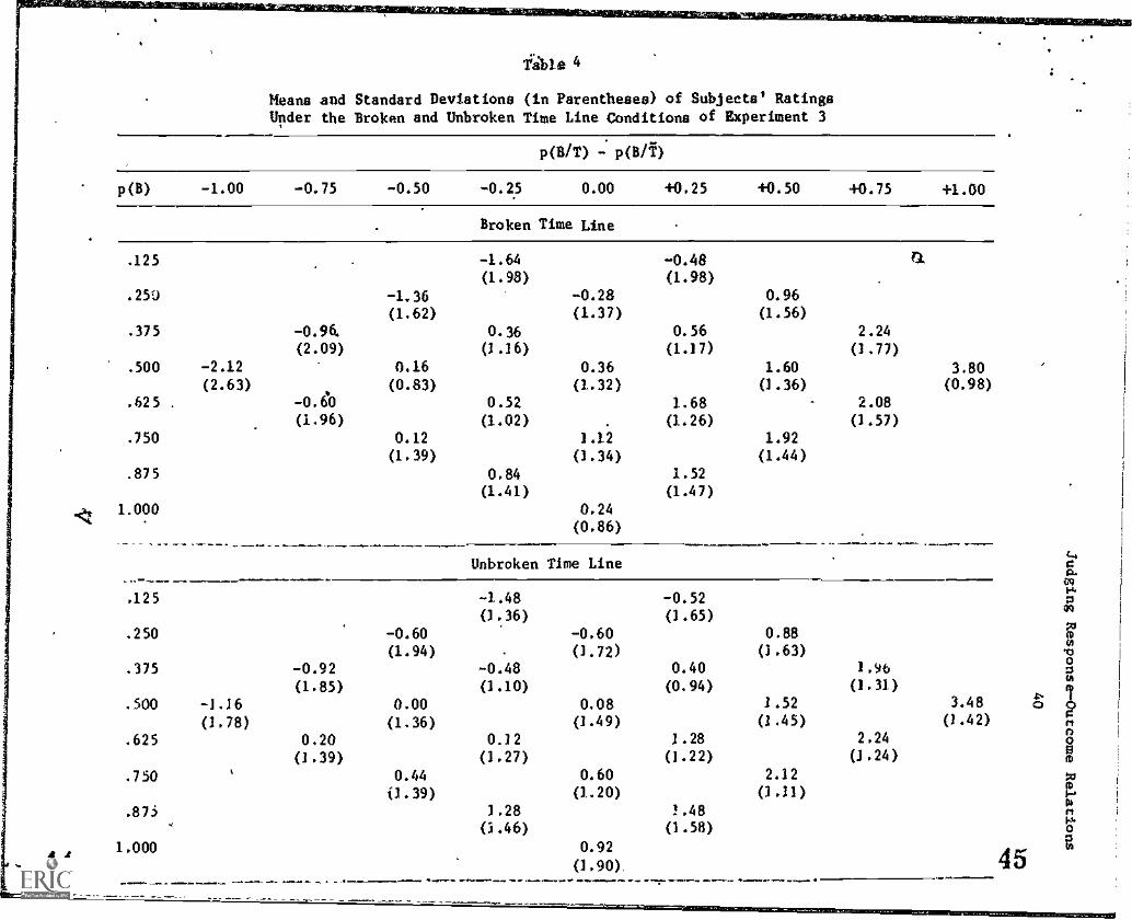
male 4

Means and Standard Deviations (in Parentheses) of Subjects' RatingsUnder the Broken and Unbroken Time Line Conditions of Experiment 3

p(B/T) p(B/f)

p(B) -1.00 -0.75 -0.50 -0.25 0.00 +0.25 +0.50 +0.75 +1.00

Broken Time Line

.125 -1.64 -0.48(1.98) (1.98)

.250 -1.36 -0.28 0.96(1.62) (1.37) (1.56)

.375 -0.96. 0.36 0.56 2.24

(2.09) (1.16) (1.17) (1.77)

.500 -2.12 0.16 0.36 1.60 3.80(2.63) (0.83) (1.32) (1.36) (0.98)

.625 . -0.60 0.52 1.68 2.08(1.96) (1.02) (1.26) (1.57)

.750 0.12 1.12 1.92(1.39) (1.34) (1.44)

.875 0.84 1.52(1.41) (1.47)

1.000 0.24(0.86)

..111.11.11.110.

Unbroken Time Line-

.125 -1.48 -0.52

(3.36) (1.65)

.250 -0.60 -0.60 0.88

(1.94) (3.72) (1.63)

.375 -0.92 -0.48 0.40 3.96

(1.85) (1.10) (0.94) (1.31)

.500 -1.16 0.00 0.08 1.52 3.48

(1.78) (1.36) (1.49) (1.45) (3.42)

.625 0.20 0.12 1.28 2.24

(1.39) (1.27) (1.22) (i.24)

.750 0.44 0.60 2.12

(1.39) (3.20) 0.11).875 3.28 1.48

(a .46) (1.58)

1.000 0.92

44 (1.90).

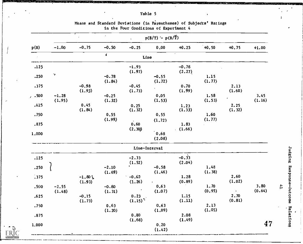
Table 5

Means and Standard Deviations (in Parentheses) of Subjedte Ratings

in the Pour Conditions of Experiment 4

p(8) -1.00 -0.75 -0.50

4

.125

....250 -0.78

(1.84)

.375 -0.98

(1.93)

.500 -1.28 -0.25(1.95) (1.32)

.625 0,45(1.84)

.750 0.55

(1.99)

.875

1.000

.125

.250 -2.10(1.69)

.375 -1.801(1.93)

.500 -2.55 -0.80(1.48) (1.31)

.625 -0.15

(1.73)

.750 0.63(1.20)

.875

1.000

P(BIT) '- p(E/T)

-0.25 0.00 40.25

Line

-1.93 -0.78(1.97) (2.27)

-0.55(1.72)

-0.45(1.73)

0.25(1.32)

0..60(2.34)

0.70

(1.99)0.05

(1.53)1.23(1.33)

0.55

(1.72)1.83(1.66)

0.68

(2.08)

Line-Interval

-2.33(1.52)

' -0.58(1.46)

-0.63

(1.26) .

0.63

(1.07)0.23(1.15)s

0.63

(1.09)0.80(1.68)

0.20

(1.42)

-0.i3(2.04)

1.28(0.89)

1.15

(1.11)

2.08(1.49)

40.50 40.75 +1.00

1.15

(1.77)

2.13

(1.60)1.58 3.45

(1.53) (1.16)

2.25(1.32)

1.60

(1.77)

1.48

(1.38)

2.60(1.02)

1.70 3.80 t'-a

(0.95) . (0.64)

2.70(0.81)

2.13

(1.05)

47

1.... .Pmrbi.

i

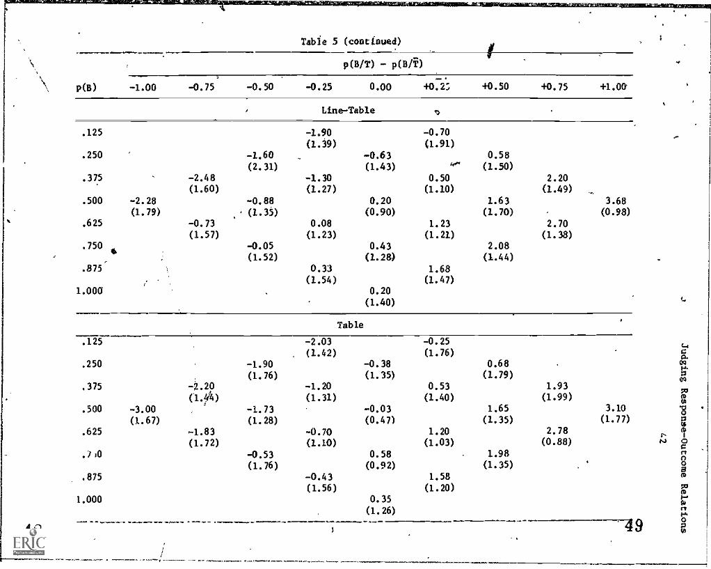
Table 5 (continued)

p(B/T) - p(0)I

p(B) -1.00 -0.75 -0.50 -0.25 0.00 +072: +0.50 +0.75 +1.00

Line-Table i.

125 -1.90 -0.70

(1.39) (1.91)

.250 -1.60 -0.63 0.58(2.31) (1.43) ke. (1.50)

.375. -2.48 -1.30 0.50 2.20

(1.60) (1.27) (1.10) (1.49)

.500 -2.28 -0.88 0.20 1.63 3.68

(1.79) . (1.35) (0.90) (1.70) (0.98)

.625 -0.73 0.08 1.23 2.70(1.57) (1.23) (1.21) (1.38)

.750 -0.05 0.43 2.084

(1.52) (1.28) (1.44)

.875 0.33 1.68

(1.54) (1.47)1.000 . 0.20

(1.40)

Table

.125 -2.03 -0.25

(1.42) (1.76)

.250 -1.90 -0.38 0.68(1.76) (1.35) (1.79)

.375 -2.20 -1.20 0.53 1.93

(1 .,W4) (1.31) (1.40) (1.99)

.500 -3.00 -1.73 -0.03 1.65 3.10

(1.67) (1.28) (0.47) (1.35) (1.77)

.625 -1.83 -0.70 1.20 2.78

(1.72) (1.10) (1.03) (0.88)

./J0 -0.53 0.58 1.98

(1.76) (0.92) (1.35)

.875 -0.43 1.58

(1.56) (1.20)

1.000 0.35

(1.26)

48

.

ow

f..

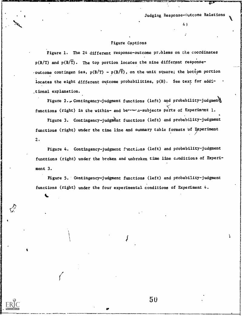
Judging Response-outcome Relations

43

Figure Captions

Figure 1. The 24 different response-outcome prJblems on the coordinates

p(B/T) and p(B/1). The top portion locates the nine different response -

- outcome contingen ies, p(B/T) p(B /T), on the-unit square; the bottom portion

locates the eight different outcome probabilities, p(B). See text for addi-

,t ional explanation.

Figure 2. io Contingency-judgment functions (left) and probability-judgmeA

functions (right) in the within- and be*0,a-subjects parts of Experiment 1.

Figure 3. Contingency-judgmlint functions (left) and probability-judgment

functions (right) under the time line and summary table formats of reriment

2.

Figure 4. Contingency-judgment fncti,:ms (left) and probability-judgment

functions (right) under the broken and unbroken time line c4nditions of Experi-

ment 3.

Figure 5. Contingency-judgment functions (left) and probability-Judgment

functions (right) under the four experimental conditions of Experiment 4.

1'

I

I

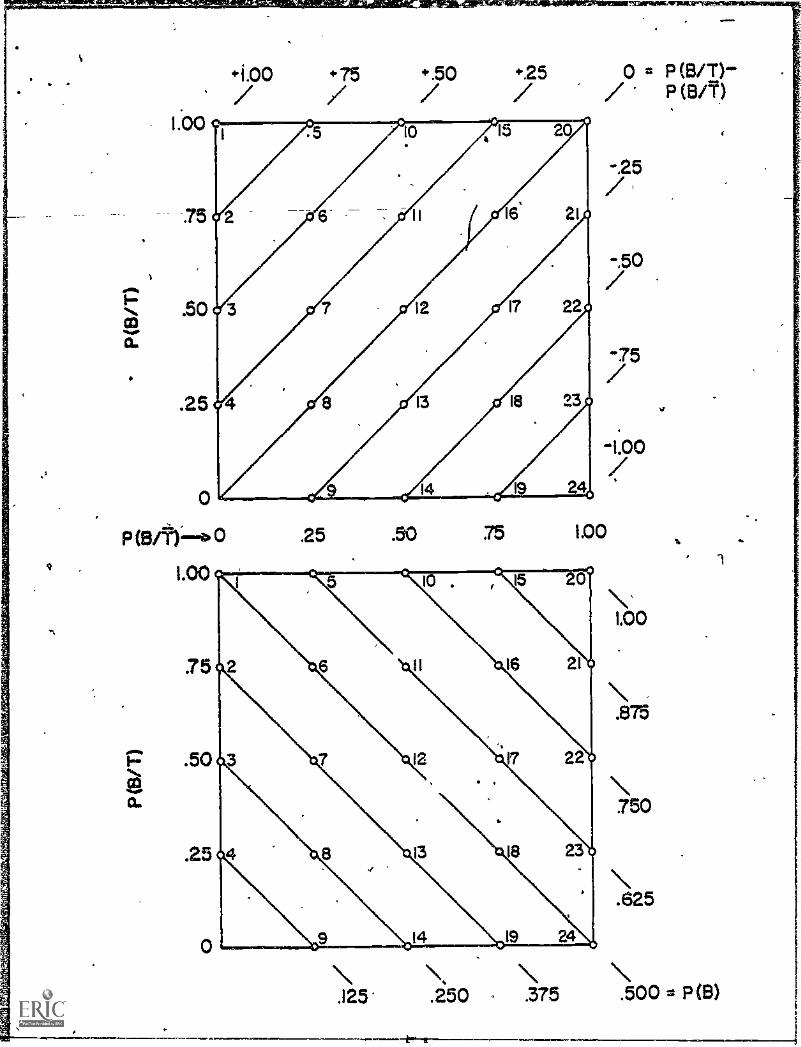
.50 +25 0 a P (B/T)/ / P EEO)

-25/-.50/

.25 .50 75

-1.00

L00

/

\100

.875

.750

.625

\ \J25 .250 .375 .500 2 NB)

1

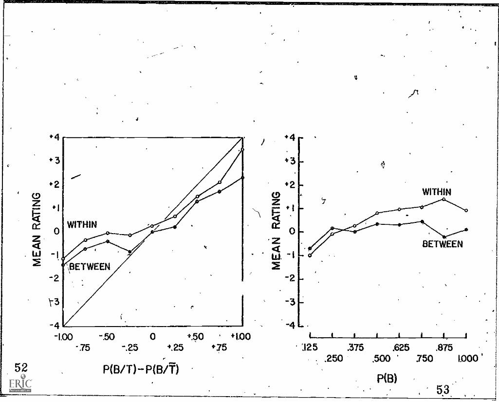
4!

410

WITHIN

WITHIN

r3e

4100 .50 0 .50 ' +100

-75 .25 .25 75

52 P03/11-PCBI)

i

4

BETWEEN

i_i_i_____iiik_i'i25 .375 .625 .875

.250 .500 750 1.000

P(B). 5,3

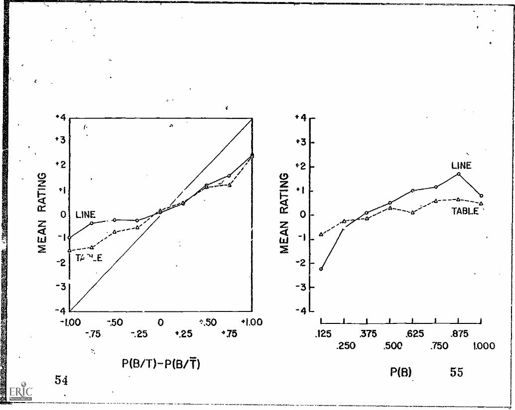
0zF.4titz4tLi2

-41.00 -,50 0 t.50 .1.00 1.._ii_i_____1, __

-.75 -.25 *.25 .75 .125 .375 .625 .875.250 .500 .750 1.000

54P(BiT)-P(B/f)

P(B) 55

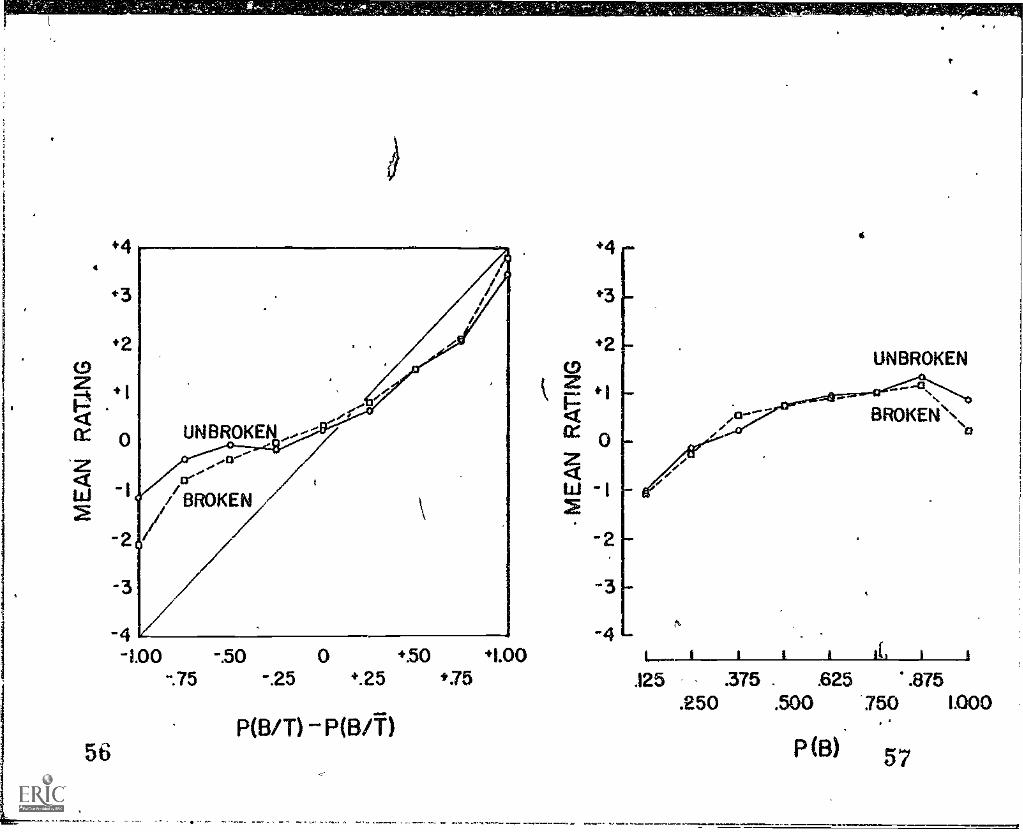
4

-4"-WO -.50 0 +.50 +1.00

-.75 -.25 '.25 +.75

Patin -1303/T)56

42UNBROKEN

C..9

4 .0 BROKEN\Ce .'4 .'W2

ft

1_,I I II ILI i.125 .375. .625 ..1375

.250 .500 '750 1.000

NB) 57

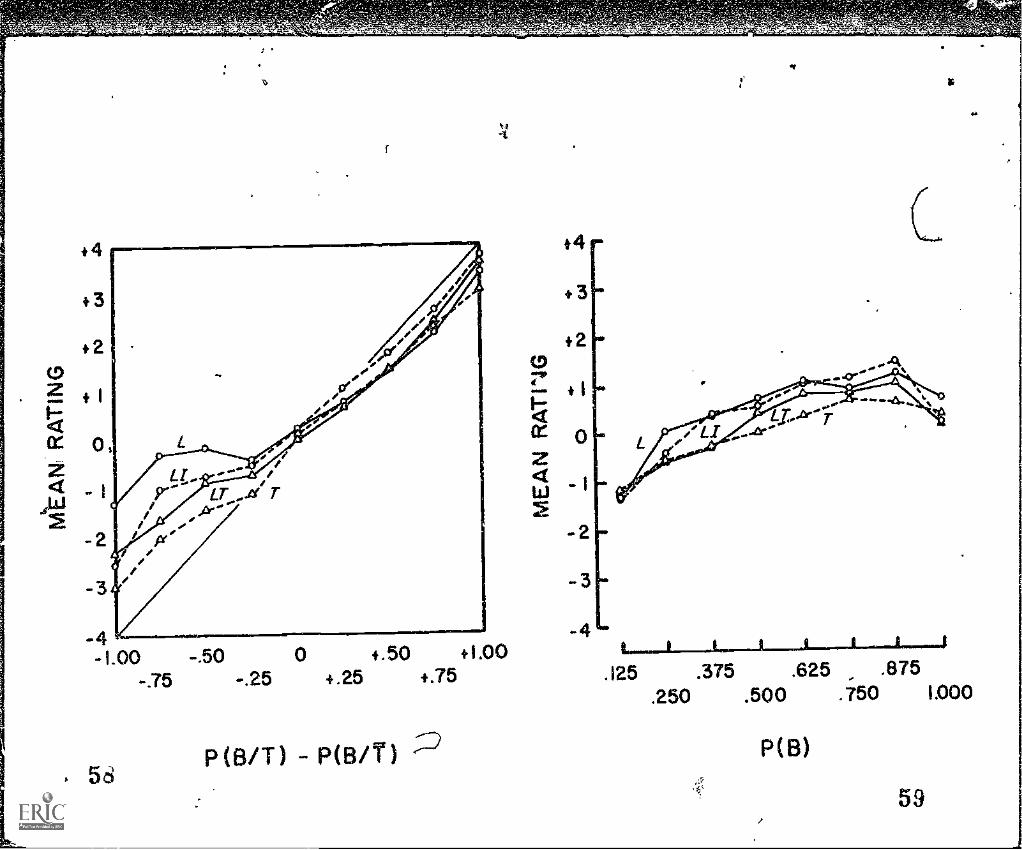
-4-1.00 -.50 0 +.50 +1.00

-.75 -.25 +.25 +.75

58P(B/T)-P(3/T)

c

.125 .375 .625 .875.250 .500 .750 1.000

NB)

59

MKS AGENCY - ERIC

Documents

Transcript of MKS AGENCY - ERIC