RESEARCH ARTICLE10.1002/2016JC011650

Mixing and phytoplankton dynamics in a submarine canyon inthe West Antarctic PeninsulaFilipa Carvalho1, Josh Kohut1, Matthew J. Oliver2, Robert M. Sherrell1,3, and Oscar Schofield1

1Department of Marine and Coastal Sciences, Rutgers University, New Brunswick, New Jersey, USA, 2College of Earth,Ocean and Environment, University of Delaware, Lewes, Delaware, USA, 3Department of Earth and Planetary Sciences,Rutgers University, Piscataway, New Jersey, USA

Abstract Bathymetric depressions (canyons) exist along the West Antarctic Peninsula shelf and havebeen linked with increased phytoplankton biomass and sustained penguin colonies. However, the physicalmechanisms driving this enhanced biomass are not well understood. Using a Slocum glider data set withover 25,000 water column profiles, we evaluate the relationship between mixed layer depth (MLD,estimated using the depth of maximum buoyancy frequency) and phytoplankton vertical distribution. Weuse the glider deployments in the Palmer Deep region to examine seasonal and across canyon variability.Throughout the season, the ML becomes warmer and saltier, as a result of vertical mixing and advection.Shallow ML and increased stratification due to sea ice melt are linked to higher chlorophyll concentrations.Deeper mixed layers, resulting from increased wind forcing, show decreased chlorophyll, suggesting theimportance of light in regulating phytoplankton productivity. Spatial variations were found in the canyonhead region where local physical water column properties were associated with different biologicalresponses, reinforcing the importance of local canyon circulation in regulating phytoplankton distributionin the region. While the mechanism initially hypothesized to produce the observed increases in phytoplank-ton over the canyons was the intrusion of warm, nutrient enriched modified Upper Circumpolar Deep Water(mUCDW), our analysis suggests that ML dynamics are key to increased primary production over submarinecanyons in the WAP.

1. Introduction

The cross-shelf canyon systems in the West Antarctic Peninsula (WAP) are considered biological ‘‘hot-spots’’ because they are associated with penguin chick rearing locations [Erdmann et al., 2011; Fraser andTrivelpiece, 1996]. The association of penguin colonies with deep submarine canyons has led to thehypothesis that phytoplankton productivity is enhanced as a result of water column dynamics in the canyonheads [Schofield et al., 2013]. The presence of the UCDW has been linked to increased phytoplankton productivity[Kavanaugh et al., 2015; Pr�ezelin et al., 2000; Pr�ezelin et al., 2004] which supports a productive regional food web[Schofield et al., 2010], yet the physical mechanisms driving phytoplankton blooms in these canyons are not wellunderstood.

The canyons in the WAP are shelf-incising [Harris and Whiteway, 2011], and often connect the off-shelf regionto the coast. Heat transport facilitated by cross-shelf canyons/troughs is enhanced by mixing particularlydue to tides [Allen and de Madron, 2009]. Small-scale roughness in canyons can be responsible for much ofthe internal tidal energy [Kunze et al., 2002], which tends to be enhanced in canyons. Additionally theseregions have enhanced internal waves with periods shorter than that of tides, and has been associated withthe vertical mixing over the slope and shelf waters [Bruno et al., 2006]. Tides in these canyons also appear to beimportant for penguin foraging behavior [Oliver et al., 2013] and krill swarms [Bernard and Steinberg, 2013].

These canyons allow UCDW to penetrate across the shelf, providing warmer [Martinson and McKee, 2012;Martinson et al., 2008] and nutrient-enriched water to mix with coastal surface waters [Arrigo et al., 2015;Pr�ezelin et al., 2000; Pr�ezelin et al., 2004]. The presence of these canyons has been connected to locallyincreased sea surface temperature (SST), reduced sea ice coverage, and increased diatom biomass [Kava-naugh et al., 2015]. Using a model, Allen et al. [2001] showed that the formation of an eddy over the head ofa canyon trapped passive particles such as phytoplankton and small zooplankton in that location.

Key Points:� Underwater gliders observe

phytoplankton dynamics in Antarcticcoastal seas� Mixed layer depth and water stability

as key driver of seasonalphytoplankton blooms� Contrary to what was initially

hypothesized, mUCDW does notseem to play an important role in thephytoplankton spring bloom in thecanyon

Correspondence to:F. Carvalho,filipa@marine.rutgers.edu

Citation:Carvalho, F., J. Kohut, M. J. Oliver,R. M. Sherrell, and O. Schofield (2016),Mixing and phytoplankton dynamicsin a submarine canyon in the WestAntarctic Peninsula, J. Geophys. Res.Oceans, 121, 5069–5083, doi:10.1002/2016JC011650.

Received 14 JAN 2016

Accepted 1 JUL 2016

Accepted article online 5 JUL 2016

Published online 24 JUL 2016

VC 2016. The Authors.

Journal of Geophysical Research:

Oceans published by Wiley Periodicals,

Inc. on behalf of American Geophysical

Union.

This is an open access article under the

terms of the Creative Commons

Attribution-NonCommercial-NoDerivs

License, which permits use and

distribution in any medium, provided

the original work is properly cited, the

use is non-commercial and no

modifications or adaptations are

made.

CARVALHO ET AL. PHYTOPLANKTON DYNAMICS IN WAP CANYON 5069

Journal of Geophysical Research: Oceans

PUBLICATIONS

Globally, light and nutrients are key drivers of a bloom, but their relative importance in primary productiondepends on the region and the role of local stratification. Light is a key factor regulating phytoplanktongrowth in polar regions, including the WAP. Several studies have linked shallower mixed layer depths(MLD), which increases the overall light available to phytoplankton [Holm-Hansen and Mitchell, 1991; Mitchelland Holm-Hansen, 1991; Moline and Prezelin, 1996; Sakshaug et al., 1991], with increased phytoplankton bio-mass, especially diatoms [Fragoso and Smith, 2012]. Increased irradiance and vertical stratification have alsobeen positively correlated with increased diatom biomass [Mitchell and Holm-Hansen, 1991; Nelson andSmith, 1991], especially during early spring season [Fragoso and Smith, 2012]. Macronutrients are generallyabundant throughout the WAP [Ducklow et al., 2012; Serebrennikova and Fanning, 2004] and although theyshow marked seasonality [Clarke et al., 2008], in most cases they do not seem to limit phytoplankton growth[Holm-Hansen and Mitchell, 1991]. Micronutrients such as iron do not seem to limit primary production inthe coastal waters of the WAP where canyon heads are located either [Annett et al., 2015; Helbling et al.,1991; Martin et al., 1990], but available data are limited.

It is important to understand the link between some of the physical drivers, like stratification and MLD, andphytoplankton dynamics as the higher trophic levels are dependent on primary producers [Schofield et al.,2010]. In this work, we characterize the phytoplankton dynamics in submarine canyons in the WAP usingPalmer Deep Canyon (PD) as a focused study area. Here we describe, both temporally and spatially, the phy-toplankton spring bloom at PD, using a 6 year Slocum glider dataset. The high spatial and temporal resolu-tion sampling provides a detailed analysis of the phytoplankton and physical dynamics at the head of asubmarine canyon in the WAP. While the mechanism initially hypothesized to produce the observedincreases in phytoplankton over the canyons was the intrusion of warm, nutrient-enriched mUCDW [Pr�ezelinet al., 2000; Pr�ezelin et al., 2004; Schofield et al., 2013], our analysis suggests that ML dynamics are key toincreased primary production over submarine canyons in the WAP.

2. Materials and Methods

2.1. Slocum GlidersSlocum electric gliders are a robust tool to map in high-resolution the upper water column properties in dif-ferent environments [Schofield et al., 2007] including polar regions [Kohut et al., 2013; Oliver et al., 2013;Schofield et al., 2013]. These 1.5 m torpedo-shaped buoyancy-driven autonomous underwater vehicles pro-vide high-resolution surveys of the physical and bio-optical properties of the water column [Schofield et al.,2007]. Data were collected using both shallow (100 m depth range) and deep (1000 m) gliders. However,only data above 100 m were considered for this analysis as we are focusing on processes within the eupho-tic zone. All gliders were equipped with a Seabird Conductivity-Temperature-Depth (CTD) sensor and WETLabs Inc. Environmental Characterization Optics (ECO) pucks, which measured chlorophyll-a fluorescence,and optical backscatter at 470, 532, 660, and 700 nm. Glider based conductivity, temperature, and depthmeasurements were compared with a calibrated ship CTD sensor on deployment and recovery to ensuredata quality, as well as with a calibrated laboratory CTD prior to deployment. Glider profiles were binnedinto 1 m bins and assigned a midpoint latitude and longitude.

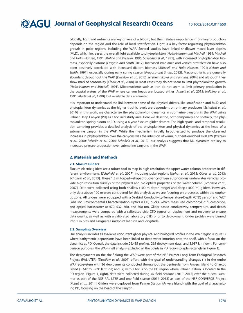
2.2. Sampling OverviewOur analysis includes all available concurrent glider physical and biological profiles in the WAP region (Figure 1)where bathymetric depressions have been linked to deep-water intrusion onto the shelf, with a focus on thedynamics at PD. Overall, the data include 26,455 profiles, 265 deployment days, and 3,937 km flown. For com-parison purposes, the WAP-shelf analysis excluded all the points in PD region (purple rectangle in Figure 1).

The deployments on the shelf along the WAP were part of the NSF Palmer-Long-Term Ecological ResearchProject (PAL-LTER) [Ducklow et al., 2007] effort, with the goal of understanding changes (1) in the entireWAP ecosystem with 26 deployments conducted throughout the peninsula from Anvers Island to CharcotIsland (2648 to 2698 latitude) and (2) with a focus on the PD region where Palmer Station is located. In thePD region (Figure 1, right), data were collected during six field seasons (2010–2015) over the austral sum-mer as part of the NSF PAL-LTER and one field season (2014–2015) as part of the NSF CONVERGE Project[Kohut et al., 2014]. Gliders were deployed from Palmer Station (Anvers Island) with the goal of characteriz-ing PD, focusing on the head of the canyon.

Journal of Geophysical Research: Oceans 10.1002/2016JC011650

CARVALHO ET AL. PHYTOPLANKTON DYNAMICS IN WAP CANYON 5070

PD (Figure 1, right), a cross-shelf canyon bathymetrically similar to others in the WAP, is associated withlarge penguin colonies [Fraser and Trivelpiece, 1996; Schofield et al., 2013]. PD extends approximately 22 kmin length and 10 km across with a maximum depth of 1420 m. Over the head of the canyon, there is evi-dence of increased primary production [Kavanaugh et al., 2015] and localized penguin foraging [Oliver et al.,2013]. Our study will describe glider data collected over varying spatial scales from the WAP shelf, to PD,and, at the smallest scale, the head of PD.

2.3. Mixed Layer Depth EstimationFor each profile, MLD was determined by finding the depth of the maximum water column buoyancy fre-quency, max (N2). A quality index (Equation 1) following Lorbacher et al. [2006] was used to quantify theuncertainty in the MLD estimate, and to filter out profiles where MLD was not resolved. Using

QI512rmsd qk2qð Þj H1 ;HMLDð Þ

rmsd qk2qð Þj H1;1:53HMLDð Þ(1)

where qk is the density at a given depth (k) and rmsd () denotes the standard deviation of from the verticalmean q from H1, the first layer near the surface, to the MLD or 1.5xMLD. This index evaluates the quality ofthe MLD computation, where MLD was determined with certainty (QI> 0.8), determined but with someuncertainty (0.5<QI< 0.8) or not determined (QI< 0.5). This index does not take into account the strengthof stratification, rather it indicates that there is a homogeneous layer present and the MLD calculated isclose to the lower boundary of that vertically uniform surface layer. Higher QI are observed during summerand fall, where sharp gradients at the base of the seasonal mixed layer are present [Lorbacher et al., 2006].

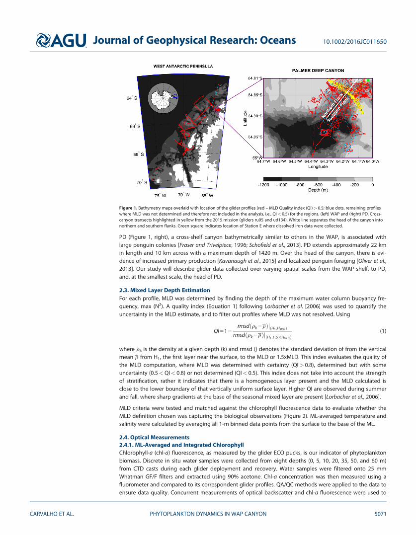
MLD criteria were tested and matched against the chlorophyll fluorescence data to evaluate whether theMLD definition chosen was capturing the biological observations (Figure 2). ML-averaged temperature andsalinity were calculated by averaging all 1-m binned data points from the surface to the base of the ML.

2.4. Optical Measurements2.4.1. ML-Averaged and Integrated ChlorophyllChlorophyll-a (chl-a) fluorescence, as measured by the glider ECO pucks, is our indicator of phytoplanktonbiomass. Discrete in situ water samples were collected from eight depths (0, 5, 10, 20, 35, 50, and 60 m)from CTD casts during each glider deployment and recovery. Water samples were filtered onto 25 mmWhatman GF/F filters and extracted using 90% acetone. Chl-a concentration was then measured using afluorometer and compared to its correspondent glider profiles. QA/QC methods were applied to the data toensure data quality. Concurrent measurements of optical backscatter and chl-a fluorescence were used to

Figure 1. Bathymetry maps overlaid with location of the glider profiles (red – MLD Quality index (QI)> 0.5; blue dots, remaining profileswhere MLD was not determined and therefore not included in the analysis, i.e., QI< 0.5) for the regions, (left) WAP and (right) PD. Cross-canyon transects highlighted in yellow from the 2015 mission (gliders ru05 and ud134). White line separates the head of the canyon intonorthern and southern flanks. Green square indicates location of Station E where dissolved iron data were collected.

Journal of Geophysical Research: Oceans 10.1002/2016JC011650

CARVALHO ET AL. PHYTOPLANKTON DYNAMICS IN WAP CANYON 5071

correct for light-dependent effects. Given the high linear correlation found between backscatter and chloro-phyll-a fluorescence (R2 between 0.76 and 0.95 for all deployments), a correction was applied to the latterto account for nonphotochemical quenching [Behrenfeld et al., 2005]. Linear regressions were calculated bydeployment using all the measurements taken between 20 and 40 m, below the light influenced chl-a val-ues and above the possible sedimentary (deep) sources of backscatter. Slope and intercept were calculatedand used to correct chlorophyll from the surface to the chlorophyll maximum in each profile. No chlorophyllmaxima were found shallower than 15 m.

Integrated and averaged chlorophyll from our defined MLD to the surface were determined using the trape-zoid method. Chl-a concentration was calculated for each 1 m bin and a cumulative value from the surfacedown to the MLD was calculated to determine the ML-integrated chlorophyll. The ML-averaged chlorophyllwas determined by dividing the ML-integrated chlorophyll by the depth of the mixed layer.2.4.2. Chlorophyll DepthA model-2 regression was used to compare the MLD with the lower boundary of the surface chlorophyllfluorescence layer. Following a method adapted from the maximum angle principle [Chu and Fan, 2011],the depth of lower boundary of chlorophyll was estimated (referred to as chlorophyll depth in Figure 2).Here we apply the same principle using the maximum angle, as we are interested in calculating the depthat which the chlorophyll profile starts decreasing. Using a vector of n 5 7 data points, the depth of the max(tanh) of the chlorophyll profile was determined and used as the chlorophyll depth.

2.5. ClimatologyOne of the main goals of this study is to characterize the physical setting and to map the seasonal phyto-plankton dynamics at the head of the PD by taking advantage of the high spatial and temporal glider

Figure 2. (top row) h-S for the two areas shown in Figure 1: (a, c) WAP, and (b, d) Palmer Deep Canyon. All data collected below 100 m areplotted in black. Color indicates depth of the water column measurement (upper 100 m of the water column). Primary water masses sam-pled are indicated and labeled (WW 5 Winter Water; AASW 5 Antarctic (summer) Surface Water; mUCDW 5 modified Upper CircumpolarDeep Water; and the regional ACC-core UCDW. (bottom row) Scatter plots comparing depth of the mixed layer (MLD) with the depth ofthe lower boundary of the chlorophyll profile for all glider profiles with Quality Index (QI) over 0.5. Shaded region represents 95% confi-dence intervals (CI) for each region. Trend lines are shown for each area and each quality index. Line 1:1 shown in green. A quality index of0.5 was also applied to chlorophyll (QIchl) profiles and only profiles with QIchl> 0.5 are shown above. Color of the dots represents normal-ized stability, i.e., the stability frequency at the depth of the ML divided by the median stability of that region.

Journal of Geophysical Research: Oceans 10.1002/2016JC011650

CARVALHO ET AL. PHYTOPLANKTON DYNAMICS IN WAP CANYON 5072

coverage. Using a 6 year data set of glider deployments (13,972 profiles after all filters applied), MLDs werecalculated for each individual profile and daily MLD averages were calculated for temperature, salinity andchlorophyll by averaging all the values between the surface and the base of the MLD.

Wind and Photosynthetic Available Radiation (PAR) data were collected from an automated weather station(AWS) at Palmer Station, on Anvers Island. Daily averages were calculated using 2 min data.

2.6. Seawater Iron MethodsSurface water was collected at LTER Station E (6.5 km NE of the head of PD), at eight time points between 5January and 9 March 2015. Samples were cleanly collected in duplicate from a Zodiac inflatable boat usingall-polypropylene syringes and filtered directly into 60 mL LDPE bottles (NalgeVR ) using 25mm Acrodisc(PallVR ) 0.45 mm pore size syringe filters, within minutes of sample collection. The resulting samples werestored at 48C until arrival at Rutgers University, where they were acidified to pH�2.0 with ultrapure HCl(Fisher OptimaVR , concentration in seawater 0.012 M). The mean of the duplicates is reported if they agreewithin 15% (difference about the mean), otherwise the lower of the two values is reported.

Seawater samples were prepared for analysis of dissolved Fe and other trace metals at Rutgers Universityusing the commercially available version of an automated preconcentration and matrix elimination system(SeaFAST picoVR , ESI, Omaha, NB) which operates on the same principle as reported in Lagerstr€om et al.[2013], and employs the method of isotope dilution, but collects eluates offline rather than directly analyz-ing online.

The eluate solutions, 25-fold concentrates of the trace metals in the sample but with greatly reduced majorion concentrations, were analyzed in medium resolution on a Thermo Element-1 HR-ICP-MS. Determinedprocess blanks for Fe typically averaged 0.040 nM and precision was 1–3% standard deviation about themean. Accuracy was verified by repeated analysis of reference seawater materials (SAFe S and D2, GEOTRA-CES S, and D), which showed agreement within one standard deviation of the consensus values.

2.7. Cross-Canyon AnalysisTo better understand the across canyon spatial variability in MLD and chlorophyll, a 1 month long glidermission was designed with a repeated transect (yellow, Figure 1) that crossed the head of the canyon per-pendicularly to its deep channel axis (64848.7’S and 64817.9’W to 64853.7’S and 6484.2’W, corresponding tothe northern and southernmost extreme of the transect, respectively). Gliders used for this temporal/spatialstudy were both shallow gliders (ru05 and ud134) rated to 100 m. The first glider (ud134) was deployed 6January 2015 and performed six full transects before ru05 took over its mission of surveying the head of thecanyon. The second glider was recovered, brought back to Palmer Station, and redeployed twice more dur-ing its mission to replace batteries and resume the cross-canyon mission. Final recovery took place on 8 Feb-ruary 2015. Gliders repeated transects across the head of the canyon 39 times throughout their missions,taking an average of 16 h to complete each cross section. The orientation of PD was used to divide (Figure1, white line) the head of the canyon into two regions, the northern and the southern flanks.

3. Results

3.1. Physical Properties Around the Palmer Deep CanyonGliders were able to map many of the key water masses during the austral summer in the WAP shelf andPD region (top plots of Figure 2). The glider profiles over six field seasons identified the Antarctic SurfaceWater (AASW), Winter Water (WW), and modified Upper Circumpolar Deep Water (mUCDW). The core-UCDW seen immediately offshore of the WAP shelf (1.7� T� 2.13; 34.54� S� 34.7, following Martinsonet al. [2008]) was not present in the canyon; instead the canyon was characterized by a modified colder andfresher mUCDW water mass. This mUCDW extended to depths below 100 m. A second water mass presentin PD was the WW (or Tmin, minimum temperature), defined by T�21.28C and 33.85� S� 34.13. The WWrepresents the remnants of the mixed-layer water from the previous winter [Martinson et al., 2008] and wasfound over a range of depths. Above the WW was the AASW (seen in the blue colors of Figure 2). In the can-yon, AASW showed a wider range of temperature, salinity, and depth. In both the WAP and PD, this watermass was freshest of all the water masses present. The main differences between the PD and the WAP shelf(PD profiles were excluded from the latter) were the absence of core-UCDW and fresh surface waters at PD.WW was found at greater depths in the WAP compared to the canyon.

Journal of Geophysical Research: Oceans 10.1002/2016JC011650

CARVALHO ET AL. PHYTOPLANKTON DYNAMICS IN WAP CANYON 5073

We evaluated the relationship between the MLD and chlorophyll depth with a model-2 linear regression(Figures 2c and 2d). In the canyon, the MLD-chlorophyll relationship was close to a 1:1 line with 95% confi-dence levels with the tightest regression associated with the profiles with the highest stability. Generallythe PD had shallower MLD than the WAP. Although more profiles in the WAP fell away from the 1:1 line,there were no significant differences (with a 95% CI) from that line for MLDs below 23 m.

3.2. Coupled Dynamics at Palmer Deep Canyon3.2.1. Seasonal Climatology of MLD and ChlorophyllA seasonal climatological analysis of the MLD properties (Figure 3) was conducted by averaging the databetween the surface and the corresponding ML for temperature, salinity, and chlorophyll-a fluorescence.Generally, MLD shoaled in December, reaching its shallowest depth (MLD5211 6 0.76 m) in the beginningof January. MLD remained fairly constant (above 20 m) throughout most of January, then started to deepenat the end of this month. The ML in January was generally fresher and colder and as it deepened it becamewarmer and saltier. Wind speed was fairly constant and low until late January. From then, there was increas-ing wind speed until the end of the growing season. The summer MLD reached its maximum depth(MLD 5 252 6 0.66 m) during the first week of February and then started shoaling again in early March.Both the temperature (Figure 3a) and salinity (Figure 3c) showed a very clear temporal signal. Secondaryshoaling of the ML in mid-February was accompanied by a freshening and slight cooling of the ML. The ML-averaged chlorophyll (Figure 3b) was highest when MLD was shallowest, i.e., throughout January. Goinginto February, when MLD was deepest, chlorophyll concentrations were low. ML-averaged chlorophyllshowed a direct relationship with MLD (y 5 0.136x 1 7.03; r2 5 0.42; p< 0.0002), with higher chl-a whenMLD is shallow and lower chl-a when deeper. An increase in chlorophyll was observed when MLD shoaledagain later in the season. Surface dissolved iron (Fe) concentrations (Figure 3d) at a station 6.5 km from the

Figure 3. Mixed Layer Depth (MLD) in the Palmer Deep region showing evolution on MLD throughout the spring/summer season. Colordenotes ML-averaged: (a) temperature, (b) chlorophyll, (c) salinity, and (d) ML-integrated chlorophyll. Marker size represents the standarderror of the variable in color (larger marker represents lower standard error, and vice-versa). Standard error of depth MLD is shown in thevertical bars. Averages were calculated using 13,972 individual glider profiles collected during 2010–2015 deployments. Daily averages ofwind and surface PAR are shown in Figures 3a and 3b, respectively. Surface iron measurements at Station E are shown in Figure 3d from2014–2015 season.

Journal of Geophysical Research: Oceans 10.1002/2016JC011650

CARVALHO ET AL. PHYTOPLANKTON DYNAMICS IN WAP CANYON 5074

canyon head, exhibited an inverse relationship with chlorophyll, reaching maximum values when MLD wasdeepest. Throughout the season, Fe concentrations at this station never fell below 0.6 nmol kg21.

The strength of water column stratification at the depth of the ML (max N2) was seen to vary through the sea-son (Figure 4). In January, when chlorophyll concentrations were high, the water column was more stable (Fig-ure 4b) and over the season the water column stability decreased. Stability was inversely correlated withsalinity (R2520.77, p< 0.0001), with higher stability associated with shallower MLD and lower salinities (Fig-ure 4a) suggesting the importance of sea ice melt and potentially glacial melt in phytoplankton primaryproductivity.3.2.2. Cross-Canyon VariabilityFour glider deployments, conducted over 1 month, collected high-resolution data across the head of thecanyon in PD with the goal of understanding the dynamics of the water masses in the canyon over the sum-mer season. The mission characterized the spatial variability between the northern and southern regions ofPD (Figure 1). A temporal and spatial analysis of the h-S plot is shown in Figure 5. The AASW, representedby the shallowest depths (blue), was cold and fresh in the beginning of January. As the month progressed,surface water became warmer and saltier. Winter water (T<21.28C), was present in the beginning of Janu-ary and was found in deeper waters as time progressed. Deeper water (reds) was warmer and saltier in thebeginning of January. The AASW was warmer at the beginning of February (Figure 5, last column).

Figure 4. Water stability in the Palmer Deep region using daily averages: (a) salinity and maximum of stability frequency (max N2);(b) seasonal climatology of MLD with max(N2). Averages were calculated using 13,972 individual glider profiles collected during2010–2015 deployments.

Figure 5. h-S scatter plots from ru05/ud134 gliders, comparing the water masses of Northern (N, top) and Southern (S, bottom) flanks of the head of the Palmer Deep canyon throughtime (plots left to right). Black dots represent all glider measurements (both areas) for the entire deployment. Color denotes depth of the water column measurement.

Journal of Geophysical Research: Oceans 10.1002/2016JC011650

CARVALHO ET AL. PHYTOPLANKTON DYNAMICS IN WAP CANYON 5075

Given the importance of ML structure in driving the chlorophyll, the h-S plots in Figure 5 were decomposedinto average depth profiles (Figure 6). The average temperature (b plots, middle row) and salinity (c plots,bottom row) depth profiles for each time point, were calculated and then compared between the tworegions (blue and red) at the head of the PD canyon. The top row in Figure 6 is for the average distributionand respective standard deviation for the temperature and salinity for each depth and different time peri-ods over the month. The southern region (blue, Figure 6a1) showed overall a wider range in temperatureand salinity in the beginning of January. This increased variance was especially marked in AASW, which wascharacterized by lower salinities. This trend reversed over the month with the northern region of the canyon(red) showing a wider variance in surface water properties (both temperature and salinity). Observed differ-ences were more influenced by temperature (Figures 6b126b4) than by salinity (Figures 6c126c4).Although surface temperatures were similar between regions, below the MLD, the northern region (red)had consistently lower temperatures (Figures 6b126b4) compared to the southern region. Differences ofover 0.58C, sometimes almost up to 18C, were found at depth on 20 January (Figure 6b2). Both areasshowed similar salinity profiles in January. The only salinity differences found were in February and weremostly due to deeper MLDs in the southern region.

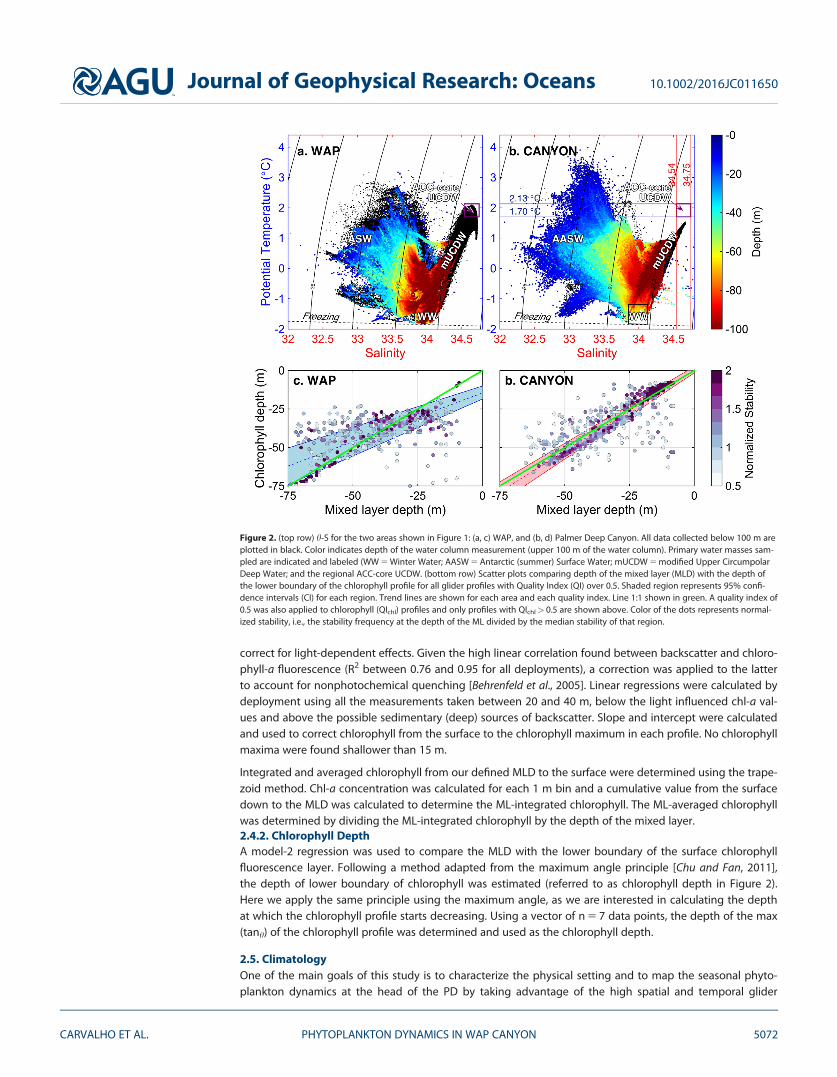
The ML-averaged and integrated chlorophyll were calculated for each profile and plotted against its corre-sponding MLD (Figure 7). Here we define the end of the bloom (21/22 January) by evaluating the evolutionof individual profiles of chlorophyll and the change of the trends between MLD and chl-a through time.This date separated two time periods, one during bloom conditions (blue, from 5 to 21 January) and thesecond during postbloom conditions (red, from 22 January to 9 February). Bloom conditions were character-ized by a clear progression from a moderately shallow (30 m) and highly productive MLD (dark blue) to aneven shallower (8 m) and less productive ML (light blue). Both ML-integrated (Figure 7a) and averaged chlo-rophyll (Figure 7b) showed similar trends. While ML-averaged chlorophyll decreased with the deepening of

Figure 6. Decomposition of the h-S diagrams from Figure 5, for Northern (red) and Southern (blue) flanks of the head of the Palmer Deep canyon: (a1–a4) average h-S diagram with aver-age (center points) and standard deviation (horizontal bars for salinity; vertical bars for temperature), (b1–b4) average temperature profile, (c1–c4) average salinity profile, with standarddeviation (shaded area), per depth for each time point.

Journal of Geophysical Research: Oceans 10.1002/2016JC011650

CARVALHO ET AL. PHYTOPLANKTON DYNAMICS IN WAP CANYON 5076

the ML and consequent ending of the bloom, ML-integrated chlorophyll increased during this postbloomcondition (Figures 7 and 9e). When comparing the two regions (northern-solid line; southern-dashed line),few differences were found.

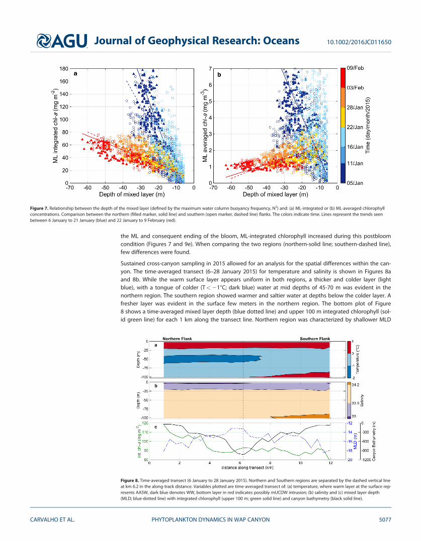
Sustained cross-canyon sampling in 2015 allowed for an analysis for the spatial differences within the can-yon. The time-averaged transect (6–28 January 2015) for temperature and salinity is shown in Figures 8aand 8b. While the warm surface layer appears uniform in both regions, a thicker and colder layer (lightblue), with a tongue of colder (T<218C; dark blue) water at mid depths of 45-70 m was evident in thenorthern region. The southern region showed warmer and saltier water at depths below the colder layer. Afresher layer was evident in the surface few meters in the northern region. The bottom plot of Figure8 shows a time-averaged mixed layer depth (blue dotted line) and upper 100 m integrated chlorophyll (sol-id green line) for each 1 km along the transect line. Northern region was characterized by shallower MLD

Figure 7. Relationship between the depth of the mixed layer (defined by the maximum water column buoyancy frequency, N2) and: (a) ML-integrated or (b) ML-averaged chlorophyllconcentrations. Comparison between the northern (filled marker, solid line) and southern (open marker, dashed line) flanks. The colors indicate time. Lines represent the trends seenbetween 6 January to 21 January (blue) and 22 January to 9 February (red).

Figure 8. Time-averaged transect (6 January to 28 January 2015). Northern and Southern regions are separated by the dashed vertical lineat km 6.2 in the along-track distance. Variables plotted are time-averaged transect of: (a) temperature, where warm layer at the surface rep-resents AASW, dark blue denotes WW, bottom layer in red indicates possibly mUCDW intrusion; (b) salinity and (c) mixed layer depth(MLD; blue-dotted line) with integrated chlorophyll (upper 100 m; green solid line) and canyon bathymetry (black solid line).

Journal of Geophysical Research: Oceans 10.1002/2016JC011650

CARVALHO ET AL. PHYTOPLANKTON DYNAMICS IN WAP CANYON 5077

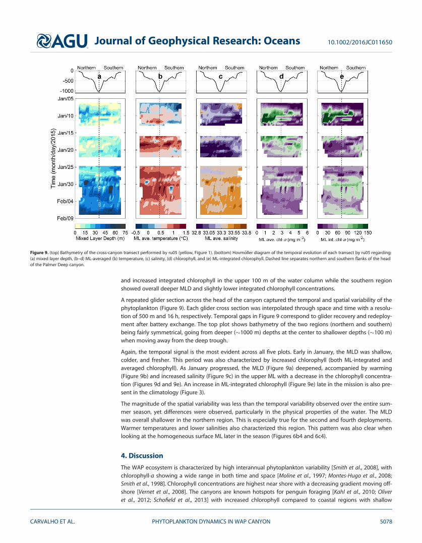
and increased integrated chlorophyll in the upper 100 m of the water column while the southern regionshowed overall deeper MLD and slightly lower integrated chlorophyll concentrations.

A repeated glider section across the head of the canyon captured the temporal and spatial variability of thephytoplankton (Figure 9). Each glider cross section was interpolated through space and time with a resolu-tion of 500 m and 16 h, respectively. Temporal gaps in Figure 9 correspond to glider recovery and redeploy-ment after battery exchange. The top plot shows bathymetry of the two regions (northern and southern)being fairly symmetrical, going from deeper (�1000 m) depths at the center to shallower depths (�100 m)when moving away from the deep trough.

Again, the temporal signal is the most evident across all five plots. Early in January, the MLD was shallow,colder, and fresher. This period was also characterized by increased chlorophyll (both ML-integrated andaveraged chlorophyll). As January progressed, the MLD (Figure 9a) deepened, accompanied by warming(Figure 9b) and increased salinity (Figure 9c) in the upper ML with a decrease in the chlorophyll concentra-tion (Figures 9d and 9e). An increase in ML-integrated chlorophyll (Figure 9e) late in the mission is also pre-sent in the climatology (Figure 3).

The magnitude of the spatial variability was less than the temporal variability observed over the entire sum-mer season, yet differences were observed, particularly in the physical properties of the water. The MLDwas overall shallower in the northern region. This is especially true for the second and fourth deployments.Warmer temperatures and lower salinities also characterized this region. This pattern was also clear whenlooking at the homogeneous surface ML later in the season (Figures 6b4 and 6c4).

4. Discussion

The WAP ecosystem is characterized by high interannual phytoplankton variability [Smith et al., 2008], withchlorophyll-a showing a wide range in both time and space [Moline et al., 1997; Montes-Hugo et al., 2008;Smith et al., 1998]. Chlorophyll concentrations are highest near shore with a decreasing gradient moving off-shore [Vernet et al., 2008]. The canyons are known hotspots for penguin foraging [Kahl et al., 2010; Oliveret al., 2012; Schofield et al., 2013] with increased chlorophyll compared to coastal regions with shallow

Figure 9. (top) Bathymetry of the cross-canyon transect performed by ru05 (yellow, Figure 1). (bottom) Hovm€oller diagram of the temporal evolution of each transect by ru05 regarding:(a) mixed layer depth, (b–d) ML-averaged (b) temperature, (c) salinity, (d) chlorophyll, and (e) ML-integrated chlorophyll. Dashed line separates northern and southern flanks of the headof the Palmer Deep canyon.

Journal of Geophysical Research: Oceans 10.1002/2016JC011650

CARVALHO ET AL. PHYTOPLANKTON DYNAMICS IN WAP CANYON 5078

bathymetry [Kavanaugh et al., 2015]. While previous studies have focused on the primary productivity overthe entire WAP [Moline and Prezelin, 1996; Montes-Hugo et al., 2010; Pr�ezelin et al., 2004], the high-resolutionsampling capabilities introduced with gliders, allowed us to conduct a detailed analysis of the canyon pri-mary production focusing on the physical forcing of the increased production observed over submarinecanyons.

4.1. The Seasonal Cycle at Palmer Deep Canyon4.1.1. Primary Water MassesA fundamental question regarding phytoplankton dynamics in the region [Schofield et al., 2013] involvesthe supply of heat and nutrients from the warm, deep water (UCDW) found at depth off the shelf. Canyonsprovide a conduit for this water to move across the shelf [Martinson et al., 2008]. No direct pathways havebeen found of ACC-core UCDW onto the Palmer Deep Canyon, so no ACC-core UCDW is present in the can-yon, but by looking at Tmax at depth, we find a modified-UCDW (relatively colder and fresher than pureUCDW) at depth. Because the bulk of the mUCDW is found at deeper depths and the gliders are usuallyonly sampling the upper 100 m of the water column, we are only partially capturing this intrusion onto thecanyon. This intrusion however is not observed to reach the euphotic zone until after the growing season.Therefore it is unlikely that it plays an important role in supplying nutrients to primary producers over thecanyon during the growing season.

The WW, identified by Tmin in the profile, was found above mUCDW. This water mass is the remnant surfacewater from the preceding winter season and is typically found at 50–60 m. WW has a very clear seasonalpattern (Figure 5), showing a well-defined and strong presence early in the season, followed by erosion bymixing with warmer water from above and below as the season progresses. The increase in solar radiationand winds, typical of the late summer season in the region, deepens the MLD, further mixing AASW withthe WW below. As the latter, saltier water mass is slowly eroded, together with the decrease in freshwaterinput later in the season due to the reduction in sea ice meltwater, a marked increase in the overall salinityof surface water is observed.4.1.2. Phytoplankton Seasonal DynamicsIn the WAP, chlorophyll-a variability has been correlated with local physical forcing such as wind, water col-umn stability, and sea ice [Saba et al., 2014]. The relationship between sea ice dynamics and biological pro-ductivity is complex. While decreasing sea ice cover can remove the shading effect of ice resulting in higherproductivity, as seen in the southern region of the WAP [Montes-Hugo et al., 2009; Saba et al., 2014], at thesame time, the decrease in fresh water input from melting sea ice will result in lower stratification and likelydeeper MLDs, which should lead to decreased primary production resulting from decreasing average lightlevels [Vernet et al., 2008].

The high variability in the timing of the sea ice retreat [Stammerjohn et al., 2008] matches the high variabilityseen in the MLD (y-axis, Figure 3) in late December. Shallower MLDs in the early growing season show bothincreased stability (Figure 4) and decreased salinity (Figure 3d). They have been associated with low windspeeds over weekly timescales [Moline, 1998; Moline and Prezelin, 1996], freshwater input from glacial and seaice melt [Meredith et al., 2008], and surface warming from incoming solar energy. The input of fresh waterfrom glacial and sea ice melting shoals the MLD, increases the stability of the water column [Garibotti et al.,2003] and restricts deep mixing. This creates a stable upper water column in which phytoplankton cells areallowed to remain in a favorable light regime [Garibotti et al., 2003; Vernet et al., 2008]. In addition, the can-yon’s proximity to land shelters the canyon head from storms and strong winds seen offshore [Hofmann et al.,1996], helping to maintain the observed shallow and stable MLD. Modeling work by Mitchell and Holm-Hansen[1991] concluded that intense phytoplankton blooms develop when MLD is shallower than 25 m, there is nolimitation by nutrients and specific loss rate is �0.3–0.35 d21, with grazing and respiration comprising over 2/3 of this loss. Although we do not have direct measurements of nutrients or loss rates at the same time as theglider profiles, our MLD and chlorophyll data match this model, with high concentrations of chlorophyllobserved in MLD of 25–30 m or shallower and declining when the MLD is deeper. Note that there was adecrease in ML-averaged chlorophyll when MLD shoals to values close to 10 m (Figure 7), suggesting somephotoinhibition processes due to high light or light limitation by self-shading [Moline et al., 1996].

The mechanisms driving the chlorophyll decrease later in the growing season remain an open question.Data show that decreases in ML-averaged chl-a are accompanied by a deepening of the ML (Figures 3

Journal of Geophysical Research: Oceans 10.1002/2016JC011650

CARVALHO ET AL. PHYTOPLANKTON DYNAMICS IN WAP CANYON 5079

and 7). Decrease in freshwater input together with increased vertical mixing from wind forcing causes MLDto deepen and water stability to decrease. Another contributor to this decreased water column stability isthe warming of WW by vertical mixing with intruding mUCDW from below. The deepening of the ML candecrease the ML-averaged chl-a concentrations by diluting a high concentration of phytoplankton over alarger depth interval; this idea is also supported by the increase in ML-integrated chl-a as MLD deepens(red line; Figure 7a), indicating there are phytoplankton below the MLD. While the deepening of the MLalone could drive down the ML-averaged chl-a concentrations as it also decreases the mean light levelsrequired for phytoplankton photosynthesis [Mitchell and Holm-Hansen, 1991], other factors, such as nutrientlimitation and grazing, can also play a role in this decrease. Although gliders do not provide in situ measure-ments of the nutrient concentrations in the water column, an inspection of historical nutrient data from theLTER Station E (6.5 km NE of the sampled area) shows that no macronutrient limitation is observed through-out the season [Ducklow et al., 2012]. The scarce micronutrient (trace metal) studies in the region make itdifficult to evaluate the micronutrient limitation question, especially regarding iron deficiency after a bloom.Iron is known to be a limiting factor controlling primary productivity in the Southern Ocean, mainly due tothe lack of efficient supply mechanisms [Boyd et al., 2012]. However, recent studies have shown that regionsin close proximity to the coast in Antarctica, such as canyon heads, are not iron limited, and that in certainparts of the WAP there is enough iron to allow the potential utilization of all macronutrients available[Annett et al., 2015]. Surface dissolved Fe:PO4 ratios measured at Station E were always above 1.1 mmolmol21, much higher than cellular Fe:P�0.2 mmol mol21 measured in Fe-limited Southern Ocean waters[Twining and Baines, 2013]. In addition, dissolved Fe was always >0.5 nmol/kg (Figure 3), higher than dis-solved Fe concentrations �0.1 nmol kg21 typical of Fe-limited waters [Sedwick et al., 2008], further support-ing our inference that Fe is not limiting phytoplankton production at the head of Palmer Canyon. Increasesin surface dissolved Fe concentrations at Station E (Figure 3) are concurrent with the deepening of the ML,indicating a potential source of iron to the surface waters. The presence of WW, acting as a physical barrierbetween the AASW and mUCDW implies that this Fe source is likely related to vertical mixing from shallowsediments or lateral advection of surface inputs such as glacial meltwater. Losses by grazing are likely a con-tributing cause of chl-a decline as canyons are known to aggregate zooplankton prey for the apex preda-tors [Bernard and Steinberg, 2013], however, we do not have concurrent zooplankton data to address thisquestion.

The timing of a secondary shoaling of the MLD in late February/early March is matched with a freshening ofthe ML and a small increase in water column stability. The rising air temperatures in the summer monthsdrive the increased fresh, glacial meltwater input onto the surface coastal waters. Concurrent with this, asecondary peak in chl-a is observed, consistent with previous work by Moline and Prezelin [1996], and areduction of dissolved Fe to intermediate values, presumably a result of decreased supply from below andincreased Fe removal in association with the chl-a increase, balancing the increased supply of Fe from gla-cial meltwater.

4.2. Palmer Deep Cross-Canyon Spatial AnalysisWhile most phytoplankton studies in the WAP canyons have focused on the temporal (seasonal and inter-annual) variability [Kavanaugh et al., 2015; Moline and Prezelin, 1996], little is known about what is drivingthe high small-scale spatial variability observed in the foraging behavior of penguins [Oliver et al., 2013].Spatial differences in phytoplankton are also likely to occur as a cyclonic eddy feature is expected to domi-nate the upper water column circulation over the canyon and to aggregate small nonmigratory species atthe head of canyons, particularly at the downstream side of the canyon [Allen et al., 2001].

Preliminary analysis of CODAR High-Frequency Radar (HFR) data at PD [Kohut et al., 2014], which providessurface maps of ocean currents, shows on average for the months of January and February, a strong North-eastward (onshore) current toward the Bismarck Straight that crosses the southern region of this study,with average speeds an order of magnitude faster than the flow that crosses the northern region. On theother hand, although a less prominent feature, a weaker Southeastward (offshore) coastal current crossesthe northern flank of the transect. Initial analysis of the mean current standard deviation shows higher vari-ability in the flow that crosses the southern region [Todoroff et al., 2015]. This highly energetic and variableflow can explain the increased variability in the water properties in that region as seen in Figures 5 and 6.This variability decreases with the temporal evolution of the water masses, with surface water becomingwarmer and saltier and with WW being warmed both from above and below. Main spatial differences in

Journal of Geophysical Research: Oceans 10.1002/2016JC011650

CARVALHO ET AL. PHYTOPLANKTON DYNAMICS IN WAP CANYON 5080

water properties can be found at depth, with the northern region showing overall colder temperatures, asevident by the presence of WW until later in the season. The southern flank shows intrusions of warm, salty,deep water likely from the onshore current forcing mUCDW onto the shelf that then mixes upward, weak-ening the signal of WW from below (Figure 8). The northern flank shows a strong presence of winter waterand a fresh water lens that comes from glacial and sea ice melt brought by the coastal current. The differ-ences in magnitude and the variability of the currents between the two regions are likely to contribute tothe stability of the MLD dynamics on local scales. With less energetic currents, the water in the northernregion is likely to show higher residence times, ideal for local primary production to occur. On the otherhand, southern region mean currents show higher variability and magnitude that can potentially impedelocal production to fully thrive as the timescales of the mean currents are shorter than the doubling time ofAntarctic phytoplankton.

Another factor known to control primary production is the availability of iron [Twining and Baines, 2013].Although there are several potential sources of iron to surface waters (glacial melt, sea-ice melt, seawaterinteraction with shallow sediments, atmospheric input and deep water upwelling), glacial meltwater hasbeen identified as one of the most important [Dierssen et al., 2002; Hawkings et al., 2014], by its volume fluxand because of the continuous yet variable supply during the growing season [Meredith et al., 2008]. Theclose proximity of canyon head systems on the WAP to the coast where glaciers are prominent features,may also contribute favorably to the increased production seen in the canyon as the increased glacial melt-water input (and pushed by the coastal current) contributes to increased water column stability and is apotential source of iron to the system [Alderkamp et al., 2015; Annett et al., 2015; Arrigo et al., 2015]. WhilemUCDW upwelling enriched with iron from sediments has been proposed as a potential source of iron tocoastal WAP regions [Annett et al., 2015], at Ryder Bay (340 km south of Palmer Deep) it was found toaccount for very little of the iron input due to the highly stratified waters during the growth season. It ishowever identified as an important source of iron over annual or longer time-scales. The same seems truefor the overall nutrient budget. Glider observations during the austral spring and summer show no evidenceof this mUCDW upwelling reaching surface waters during the growth season as there is a clear layer of WWphysically separating surface waters from the deep waters below while the bloom is present. However,this water mass is slowly warming throughout the season due to vertical mixing from above and below,contributing to the decreased water column stability. While there is no evidence of the surface waters at PDbeing limited by macro or micronutrients at any point, a drawdown in the nutrient pool is apparent whilethe bloom is thriving [Ducklow et al., 2012]. After the growth season, as the stratification weakens, mUCDWintrusions from below will replenish the surface water with both micro and macronutrients required for thefollowing year’s spring phytoplankton bloom.

5. Conclusions

Understanding the spatial and temporal variability of phytoplankton is important, especially to assess thedynamics of higher trophic levels as they are dependent on primary producers for food source. The high-resolution capabilities of gliders allow sampling and coverage at appropriate scales to evaluate phytoplank-ton dynamics. Using the 6 year glider observations over PD, we were able to describe the fine temporal andspatial variability of the phytoplankton seasonal cycle and relate it to its main physical drivers, namely MLDand water stability. Although interannual variability was observed in the data, the shoaling of the MLD inlate spring matching increased chlorophyll concentration was a pattern observed in all years sampled(2010–2015), as more light becomes available to the phytoplankton community. Following this period, asummer (February) deepening of the MLD was accompanied by decreased chlorophyll concentration.

Observations showed that MLD dynamics and chlorophyll variability were tightly coupled in both time andspace. Spatial variability was evaluated by glider transects across the head of the canyon. While MLDdynamics was similar in the northern and southern canyon regions, the physical setting observed in diffe-rent regions of the canyon, such as water column stratification and water masses present, explain some ofthe observed chlorophyll variability. Preliminary analysis of surface currents provides an insight on whatcould be driving some of the observed differences in water column structure that are key for phytoplanktondevelopment. The northern region with increased chlorophyll showed a more coastal influence, withincreased freshwater input, slower currents, and increased stratification, while the southern region with

Journal of Geophysical Research: Oceans 10.1002/2016JC011650

CARVALHO ET AL. PHYTOPLANKTON DYNAMICS IN WAP CANYON 5081

lower chlorophyll showed more influence from offshore with faster currents and more intrusions of mUCDWfrom below. However, further sampling and analysis is necessary to evaluate whether water column physicsis driving the spatial differences in chlorophyll concentrations alone or if iron supply plays a role in the sys-tem at any point in the growth season.

ReferencesAlderkamp, A., G. L. van Dijken, K. E. Lowry, T. L. Connelly, M. Lagerstr€om, R. M. Sherrell, C. Haskins, E. Rogalsky, O. Schofield, and

S. E. Stammerjohn (2015), Fe availability drives phytoplankton photosynthesis rates during spring bloom in the Amundsen Sea Polynya,Antarctica, Elementa, 3(1), 000043.

Allen, S. E., and X. D. de Madron (2009), A review of the role of submarine canyons in deep-ocean exchange with the shelf, Ocean Sci., 5(4),607–620.

Allen, S. E., C. Vindeirinho, R. E. Thomson, M. G. G. Foreman, and D. L. Mackas (2001), Physical and biological processes over a submarinecanyon during an upwelling event, Can. J. Fish. Aquat. Sci., 58(4), 671–684, doi:10.1139/cjfas-58-4-671.

Annett, A. L., M. Skiba, S. F. Henley, H. J. Venables, M. P. Meredith, P. J. Statham, and R. S. Ganeshram (2015), Comparative roles of upwell-ing and glacial iron sources in Ryder Bay, coastal western Antarctic Peninsula, Mar. Chem., 176, 21–33, doi:10.1016/j.marchem.2015.06.017.

Arrigo, K. R., G. L. van Dijken, and A. L. Strong (2015), Environmental controls of marine productivity hot spots around Antarctica,J. Geophys. Res. Oceans, 120, 5545–5565, doi:10.1002/2015JC010888.

Behrenfeld, M. J., E. Boss, D. A. Siegel, and D. M. Shea (2005), Carbon-based ocean productivity and phytoplankton physiology from space,Global Biogeochem. Cycles, 19, GB1006, doi:10.1029/2004GB002299.

Bernard, K. S., and D. K. Steinberg (2013), Krill biomass and aggregation structure in relation to tidal cycle in a penguin foraging region offthe Western Antarctic Peninsula, ICES J. Mar. Sci., 70(4), 834–849, doi:10.1093/icesjms/fst088.

Boyd, P. W., K. R. Arrigo, R. Strzepek, and G. L. van Dijken (2012), Mapping phytoplankton iron utilization: Insights into Southern Ocean sup-ply mechanisms, J. Geophys. Res., 117, C06009, doi:10.1029/2011JC007726.

Bruno, M., A. Vazquez, J. Gomez-Enri, J. M. Vargas, J. G. Lafuente, A. Ruiz-Canavate, L. Mariscal, and J. Vidal (2006), Observations of internalwaves and associated mixing phenomena in the Portimao Canyon area, Deep Sea Res., Part II, 53(11–13), 1219–1240, doi:10.1016/j.dsr2.2006.04.015.

Chu, P. C., and C. W. Fan (2011), Maximum angle method for determining mixed layer depth from seaglider data, J. Oceanogr., 67(2),219–230, doi:10.1007/s10872-011-0019-2.

Clarke, A., M. P. Meredith, M. I. Wallace, M. A. Brandon, and D. N. Thomas (2008), Seasonal and interannual variability in temperature, chlo-rophyll and macronutrients in northern Marguerite Bay, Antarctica, Deep Sea Res., Part II, 55(18–19), 1988–2006, doi:10.1016/j.dsr2.2008.04.035.

Dierssen, H. M., R. C. Smith, and M. Vernet (2002), Glacial meltwater dynamics in coastal waters west of the Antarctic peninsula, Proc. Natl.Acad. Sci. U. S. A., 99(4), 1790–1795, doi:10.1073/pnas.032206999.

Ducklow, H. W., K. Baker, D. G. Martinson, L. B. Quetin, R. M. Ross, R. C. Smith, S. E. Stammerjohn, M. Vernet, and W. Fraser (2007), Marinepelagic ecosystems: The west Antarctic Peninsula, Philos. Trans. R. Soc. B, 362(1477), 67–94.

Ducklow, H. W., A. Clarke, R. Dickhut, S. C. Doney, H. Geisz, K. Huang, D. G. Martinson, M. P. Meredith, H. V. Moeller, and M. Montes-Hugo(2012), The Marine System of the Western Antarctic Peninsula, in Antarctic Ecosystems: An Extreme Environment in a Changing World,edited by A. D. Rogers, et al., pp. 121–159, John Wiley & Sons, Ltd., Chichester, U. K., doi:10.1002/9781444347241.ch5.

Erdmann, E. S., C. A. Ribic, D. L. Patterson-Fraser, and W. R. Fraser (2011), Characterization of winter foraging locations of Adelie penguinsalong the Western Antarctic Peninsula, 2001-2002, Deep Sea Res., Part II, 58(13–16), 1710–1718, doi:10.1016/j.dsr2.2010.10.054.

Fragoso, G. M., and W. O. Smith (2012), Influence of hydrography on phytoplankton distribution in the Amundsen and Ross Seas, Antarcti-ca, J. Mar. Syst., 89(1), 19–29, doi:10.1016/j.jmarsys.2011.07.008.

Fraser, W. R., and W. Z. Trivelpiece (1996), Factors controlling the distribution of seabirds: Winter-summer heterogeneity in the distributionof ad�elie penguin populations, Antarct. Res. Ser., 70, 257–272.

Garibotti, I. A., M. Vernet, M. E. Ferrario, R. C. Smith, R. M. Ross, and L. B. Quetin (2003), Phytoplankton spatial distribution patterns alongthe western Antarctic Peninsula (Southern Ocean), Mar. Ecol. Prog. Ser., 261, 21–39, doi:10.3354/meps261021.

Harris, P. T., and T. Whiteway (2011), Global distribution of large submarine canyons: Geomorphic differences between active and passivecontinental margins, Mar. Geol., 285(1–4), 69–86, doi:10.1016/j.margeo.2011.05.008.

Hawkings, J. R., J. L. Wadham, M. Tranter, R. Raiswell, L. G. Benning, P. J. Statham, A. Tedstone, P. Nienow, K. Lee, and J. Telling (2014), Icesheets as a significant source of highly reactive nanoparticulate iron to the oceans, Nat. Commun., 5, 3929, doi:10.1038/ncomms4929.

Helbling, E. W., V. Villafane, and O. Holmhansen (1991), Effect of Iron on Productivity and Size Distribution of Antarctic Phytoplankton, Lim-nol. Oceanogr., 36(8), 1879–1885.

Hofmann, E. E., J. M. Klinck, C. M. Lascara, and D. A. Smith (1996), Water mass distribution and circulation west of the Antarctic Peninsulaand including Bransfield Strait, in Foundations for Ecological Research West of the Antarctic Peninsula, edited by R. M. Ross, E. E. Hofmannand L. B. Quetin, AGU, Washington, D. C., doi:10.1029/AR070p0061.

Holm-Hansen, O., and B. Mitchell (1991), Spatial and temporal distribution of phytoplankton and primary production in the western Brans-field Strait region, Deep Sea Res. Part A, 38(8), 961–980.

Kahl, L. A., O. Schofield, and W. R. Fraser (2010), Autonomous gliders reveal features of the water column associated with foraging by adeliepenguins, Integr. Comp. Biol., 50(6), 1041–1050, doi:10.1093/icb/icq098.

Kavanaugh, M. T., F. N. Abdala, H. Ducklow, D. Glover, W. Fraser, D. Martinson, S. Stammerjohn, O. Schofield, and S. C. Doney (2015), Effectof continental shelf canyons on phytoplankton biomass and community composition along the western Antarctic Peninsula, Mar. Ecol.Prog. Ser., 524, 11–26, doi:10.3354/meps11189.

Kohut, J., E. Hunter, and B. Huber (2013), Small-scale variability of the cross-shelf flow over the outer shelf of the Ross Sea, J. Geophys. Res.Oceans, 118, 1863–1876, doi:10.1002/jgrc.20090.

Kohut, J., K. Bernard, W. Fraser, M. J. Oliver, H. Statscevvich, P. Winsor, and T. Miles (2014), Studying the impacts of local oceanographic pro-cesses on adelie penguin foraging ecology, Mar. Technol. Soc. J., 48(5), 25–34.

Kunze, E., L. K. Rosenfeld, G. S. Carter, and M. C. Gregg (2002), Internal waves in Monterey Submarine Canyon, J. Phys. Oceanogr., 32(6),1890–1913, doi:10.1175/1520-0485(2002)032< 1890:IWIMSC>2.0.CO;2.

AcknowledgmentsWe thank the two anonymousreviewers whose suggestions helpedimprove and clarify this manuscript.The research was supported by theNational Science Foundation grantsANT-0823101 (Palmer-LTER), ANT-1327248 and ANT-1326541(CONVERGE) and ANT-1142250 (ironWAP). Filipa Carvalho was funded by aPortuguese doctoral fellowship fromFundac~ao para a Ciencia e Tecnologia(DFRH-SFRH/BD/72705/2010). Gliderdata can be accessed at ERDDAPserver at http://erddap.marine.rutgers.edu/erddap/info/. Weather data canbe access at http://oceaninformatics.ucsd.edu/datazoo/data/pallter/datasets.

Journal of Geophysical Research: Oceans 10.1002/2016JC011650

CARVALHO ET AL. PHYTOPLANKTON DYNAMICS IN WAP CANYON 5082

Lagerstr€om, M., M. Field, M. S�eguret, L. Fischer, S. Hann, and R. Sherrell (2013), Automated on-line flow-injection ICP-MS determination oftrace metals (Mn, Fe, Co, Ni, Cu and Zn) in open ocean seawater: Application to the GEOTRACES program, Mar. Chem., 155, 71–80.

Lorbacher, K., D. Dommenget, P. P. Niiler, and A. K€ohl (2006), Ocean mixed layer depth: A subsurface proxy of ocean-atmosphere variability,J. Geophys. Res., 111, C07010, doi:10.1029/2003JC002157.

Martin, J. H., S. E. Fitzwater, and R. M. Gordon (1990), Iron deficiency limits phytoplankton growth in Antarctic waters, Global Biogeochem.Cycles, 4(1), 5–12.

Martinson, D. G., and D. C. McKee (2012), Transport of warm upper circumpolar deep water onto the western Antarctic Peninsula continen-tal shelf, Ocean Sci., 8(4), 433–442, doi:10.5194/os-8-433-2012.

Martinson, D. G., S. E. Stammerjohn, R. A. Iannuzzi, R. C. Smith, and M. Vernet (2008), Western Antarctic Peninsula physical oceanographyand spatio-temporal variability, Deep Sea Res., Part II, 55(18–19), 1964–1987, doi:10.1016/j.dsr2.2008.04.038.

Meredith, M. P., M. A. Brandon, M. I. Wallace, A. Clarke, M. J. Leng, I. A. Renfrew, N. P. Van Lipzig, and J. C. King (2008), Variability in the fresh-water balance of northern Marguerite Bay, Antarctic Peninsula: Results from hwater b, Deep Sea Res., Part II, 55(3), 309–322.

Mitchell, B. G., and O. Holm-Hansen (1991), Observations of modeling of the Antartic phytoplankton crop in relation to mixing depth, DeepSea Res., Part A, 38(8), 981–1007.

Moline, M. A. (1998), Photoadaptive response during the development of a coastal Antarctic diatom bloom and relationship to water col-umn stability, Limnol. Oceanogr., 43(1), 146–153.

Moline, M. A., and B. B. Prezelin (1996), Long-term monitoring and analyses of physical factors regulating variability in coastal Antarcticphytoplankton biomass, in situ productivity and taxonomic composition over subseasonal, seasonal and interannual time scales, Mar.Ecol. Prog. Ser., 145(1–3), 143–160, doi:10.3354/meps145143.

Moline, M. A., B. B. Prezelin, and H. Claustre (1996), Light-saturated primary production in antarctic coastal waters, Antarct. J. U. S., 31(5),105–107.

Moline, M. A., B. B. Prezelin, O. Schofield, and R. C. Smith (1997), Temporal dynamics of coastal Antarctic phytoplankton: Environmentaldriving forces and impact of 1991/92 summer diatom bloom on the nutrient regimes, in Antarctic Communities: Species, Structure andSurvival, edited by B. Battaglia, J. Valencia, and D. W. H. Walton, pp. 67–72, Cambridge Univ. Press, Cambridge.

Montes-Hugo, M. A., M. Vernet, D. Martinson, R. Smith, and R. Iannuzzi (2008), Variability on phytoplankton size structure in the westernAntarctic Peninsula (1997-2006), Deep Sea Res., Part II, 55(18–19), 2106–2117, doi:10.1016/j.dsr2.2008.04.036.

Montes-Hugo, M. A., S. C. Doney, H. W. Ducklow, W. Fraser, D. Martinson, S. E. Stammerjohn, and O. Schofield (2009), Recent changes inphytoplankton communities associated with rapid regional climate change along the western Antarctic Peninsula, Science, 323(5920),1470–1473, doi:10.1126/science.1164533.

Montes-Hugo, M. A., C. Sweeney, S. C. Doney, H. Ducklow, R. Frouin, D. G. Martinson, S. Stammerjohn, and O. Schofield (2010), Seasonalforcing of summer dissolved inorganic carbon and chlorophyll a on the western shelf of the Antarctic Peninsula, J. Geophys. Res., 115,C03024, doi:10.1029/2009JC005267.

Nelson, D. M., and W. Smith (1991), The role of light and major nutrients, Limnol. Oceanogr., 36, 1650–1661.Oliver, M. J., M. A. Moline, I. Robbins, W. Fraser, D. Patterson, and O. Schofield (2012), Letting penguins lead: Dynamic modeling of penguin

locations guides autonomous robotic sampling, Oceanography, 25(3), 120–121.Oliver, M. J., A. Irwin, M. A. Moline, W. Fraser, D. Patterson, O. Schofield, and J. Kohut (2013), Adelie penguin foraging location predicted by

tidal regime switching, PLoS One, 8(1), e55163, doi:10.1371/journal.pone.0055163.Pr�ezelin, B. B., E. E. Hofmann, C. Mengelt, and J. M. Klinck (2000), The linkage between Upper Circumpolar Deep Water (UCDW) and phyto-

plankton assemblages on the west Antarctic Peninsula continental shelf, J. Mar. Res., 58(2), 165–202.Pr�ezelin, B. B., E. E. Hofmann, M. Moline, and J. M. Klinck (2004), Physical forcing of phytoplankton community structure and primary pro-

duction in continental shelf waters of the Western Antarctic Peninsula, J. Mar. Res., 62(3), 419–460.Saba, G. K., et al. (2014), Winter and spring controls on the summer food web of the coastal West Antarctic Peninsula, Nat. Commun., 5,

4318, doi:10.1038/ncomms5318.Sakshaug, E., G. Johnsen, K. Andresen, and M. Vernet (1991), Modeling of light-dependent algal photosynthesis and growth: Experiments

with the Barents sea diatoms Thalassiosira nordenskioldii and Chaetoceros furcellatus, Deep Sea Res., Part A, 38(4), 415–430.Schofield, O., et al. (2007), Slocum gliders: Robust and ready, J. Field Robot, 24(6), 473–485, doi:10.1002/rob.20200.Schofield, O., H. W. Ducklow, D. G. Martinson, M. P. Meredith, M. A. Moline, and W. R. Fraser (2010), How do polar marine ecosystems

respond to rapid climate change?, Science, 328(5985), 1520–1523.Schofield, O., et al. (2013), Penguin biogeography along the west antarctic peninsula testing the canyon hypothesis with Palmer LTER

observations, Oceanography, 26(3), 204–206.Sedwick, P. N., A. R. Bowie, and T. W. Trull (2008), Dissolved iron in the Australian sector of the Southern Ocean (CLIVAR SR3 section): Merid-

ional and seasonal trends, Deep Sea Res., Part I, 55(8), 911–925, doi:10.1016/j.dsr.2008.03.011.Serebrennikova, Y. M., and K. A. Fanning (2004), Nutrients in the Southern Ocean GLOBEC region: Variations, water circulation, and cycling,

Deep Sea Res., Part II, 51(17–19), 1981–2002, doi:10.1016/j.dsr2.2004.07.023.Smith, R. C., K. S. Baker, and M. Vernet (1998), Seasonal and interannual variability of phytoplankton biomass west of the Antarctic Peninsu-

la, J. Mar. Syst., 17(1–4), 229–243, doi:10.1016/S0924-7963(98)00040-2.Smith, R. C., D. G. Martinson, S. E. Stammerjohn, R. A. Iannuzzi, and K. Ireson (2008), Bellingshausen and western Antarctic Peninsula region:

Pigment biomass and sea-ice spatial/temporal distributions and interannual variabilty, Deep Sea Res., Part II, 55(18–19), 1949–1963, doi:10.1016/j.dsr2.2008.04.027.

Stammerjohn, S. E., D. G. Martinson, R. C. Smith, and R. A. Iannuzzi (2008), Sea ice in the western Antarctic Peninsula region: Spatiotemporalvariability from ecological and climate change perspectives, Deep Sea Res., Part II, 55(18-19), 2041–2058, doi:10.1016/j.dsr2.2008.04.026.

Todoroff, K., J. Kohut, P. Winsor, and H. Statscewich (2015), Spatial circulation patterns over Palmer Deep canyon and the effects on Ad�eliePenguin foraging, paper presented at OCEANS 2015-MTS/IEEE Washington, IEEE, Washington, D. C., 19–22 Oct.

Twining, B. S., and S. B. Baines (2013), The trace metal composition of marine phytoplankton, Ann. Rev. Mar. Sci., 5, 191–215, doi:10.1146/annurev-marine-121211-172322.

Vernet, M., D. Martinson, R. Iannuzzi, S. Stammerjohn, W. Kozlowski, K. Sines, R. Smith, and I. Garibotti (2008), Primary production within thesea-ice zone west of the Antarctic Peninsula: I-Sea ice, summer mixed layer, and irradiance, Deep Sea Res., Part II, 55(18–19), 2068–2085,doi:10.1016/j.dsr2.2008.05.021.

Journal of Geophysical Research: Oceans 10.1002/2016JC011650

CARVALHO ET AL. PHYTOPLANKTON DYNAMICS IN WAP CANYON 5083