Mixers - courses.aqsim.comcourses.aqsim.com/Analyzer/V9.5/TOTv9.5-Ch-05-Mixers--Jun17.pdf · Mixers...
25
Mixers Introduction In this chapter, we will look at how Stream Analyzer mixes two or more streams. The object is called Mixer and you will familiarize yourselves with its three mixing options, Multiplier, Ratio, and Volume. It should be noted that in previous software versions, the Multiplier option was called Ratio and the Ratio option was labeled Proportion. If you are familiar with Versions 4 and earlier, you will note this difference. We will also mix two incompatible waters using the Water Analysis objects that were created in Chapter 4. Lastly, we will perform a titration experiment using the Mixer feature. As in previous chapters, these lessons are designed around real-world situations. The Mixer object or block can be accessed from the Menu Bar by selecting Calculations > Add Mixer or by selecting the Add Mixer in the Actions Pane as shown below: Large Icon View Small Icon / List View The Mixer should not be confused with the Studio ScaleChem object called Mixing Water: Calculation List 5.1 Mixing Two Incompatible Waters.................................................................................................................2 5.2 Simple Mixer Calculation ..............................................................................................................................8 5.3 Neutralizing Two Streams .......................................................................................................................... 12 5.4 Creating a Titration Curve.......................................................................................................................... 23
Transcript of Mixers - courses.aqsim.comcourses.aqsim.com/Analyzer/V9.5/TOTv9.5-Ch-05-Mixers--Jun17.pdf · Mixers...

Mixers
Introduction
In this chapter, we will look at how Stream Analyzer mixes two or more streams. The object is called Mixer and you will familiarize yourselves with its three mixing options, Multiplier, Ratio, and Volume. It should be noted that in previous software versions, the Multiplier option was called Ratio and the Ratio option was labeled Proportion. If you are familiar with Versions 4 and earlier, you will note this difference.
We will also mix two incompatible waters using the Water Analysis objects that were created in Chapter 4. Lastly, we will perform a titration experiment using the Mixer feature. As in previous chapters, these lessons are designed around real-world situations.
The Mixer object or block can be accessed from the Menu Bar by selecting Calculations > Add Mixer or by selecting the Add Mixer in the Actions Pane as shown below:
Large Icon View
Small Icon / List View
The Mixer should not be confused with the Studio ScaleChem object called Mixing Water:
Calculation List 5.1 Mixing Two Incompatible Waters .................................................................................................................2
5.2 Simple Mixer Calculation ..............................................................................................................................8
5.3 Neutralizing Two Streams .......................................................................................................................... 12
5.4 Creating a Titration Curve .......................................................................................................................... 23

5-2 Chapter 5 Mixers Tricks of the Trade
5.1 Mixing Two Incompatible Waters
Overview
This case was begun in Chapter 4, where two water analyses, High Ca/Ba and High HCO3/SO4 were created. These waters will be mixed in this case. The potential solid phases are Ca+2, Sr+2, and Ba+2 forms of SO4
-2 and CO3-2. The exact phase that forms depends on the mixing fraction of each water.
Procedure
✓ Open the file that contains the ‘High Calcium/Barium’ and the ‘High Bicarb/Sulfate’ analyses
Each object should have a distinct label. This will be important in the next step
✓ Add a new Mixer from the Actions Pane or from the menu bar Calcualtions > Add Mixer
✓ Rename the mixer ‘Incompatible Waters’
✓ Select the Definition tab of the new mixer
There should be two streams in the Available field, Reconcile Ca/Ba and Reconcile HCO3/SO4. These are the two Reconcile objects. By comparison the Water Analysis objects are not present, because no charge balance or calculation was done at that level.
✓ Highlight both streams and add them to the Selected section.
Tricks of the Trade Chapter 5 Mixers 5-3
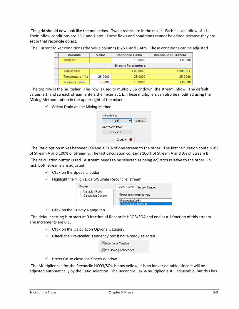
The grid should now look like the one below. Two streams are in the mixer. Each has an inflow of 1 L. Their inflow conditions are 25 C and 1 atm. These flows and conditions cannot be edited because they are set in that reconcile object.
The Current Mixer conditions (the value column) is 25 C and 1 atm. These conditions can be adjusted.
The top row is the multiplier. This row is used to multiply up or down, the stream inflow. The default values is 1, and so each stream enters the mixer at 1 L. These multipliers can also be modified using the Mixing Method option in the upper right of the mixer
✓ Select Ratio as the Mixing Method
The Ratio option mixes between 0% and 100 % of one stream to the other. The first calculation contain 0% of Stream A and 100% of Stream B. The last calculation contains 100% of Stream A and 0% of Stream B.
The calculation button is red. A stream needs to be selected as being adjusted relative to the other. In fact, both streams are adjusted;
✓ Click on the Specs… button
✓ Highlight the ‘High Bicarb/Sulfate Reconcile’ stream
✓ Click on the Survey Range tab
The default setting is to start at 0 fraction of Reconcile HCO3/SO4 and end at a 1 fraction of this stream. The increments are 0.1.
✓ Click on the Calculation Options Category
✓ Check the Pre-scaling Tendency box if not already selected
✓ Press OK to close the Specs Window
The Multiplier cell for the Reconcile HCO3/SO4 is now yellow, it is no longer editable, since it will be adjusted automatically by the Ratio selection. The Reconcile Ca/Ba multiplier is still adjustable, but this has

5-4 Chapter 5 Mixers Tricks of the Trade
the net effect of changing the total amount of flow to the system, and not just this stream, since the mixing is still based on fraction.
✓ Calculate
✓ Select the Plot tab
The plot will be blank, because there is no default variable set. You will select variables next.
✓ Select the Variables button
✓ Remove any variables from the Y1 Axis
✓ Expand the Pre-Scaling Tendencies category
✓ Double-click Dominant Pre-Scaling Tendencies to add it to the Y1 Axis
✓ Press OK and view the plot
The resulting plot is a typical fluid incompatibility. The two waters when mixed equally are predicted to reach maximum supersaturation with barite. Notice that other curves are present, but their shape cannot be seen because of the high barite value.
✓ Select the Curves button
✓ Double-click Dominant Pre-Scaling Tendencies to remove it from the Y1 Axis
✓ Expand the Pre-Scaling Tendency category
✓ Add CaCO3 (Calcite) and SrSO4 to the Y-Axis
Tricks of the Trade Chapter 5 Mixers 5-5
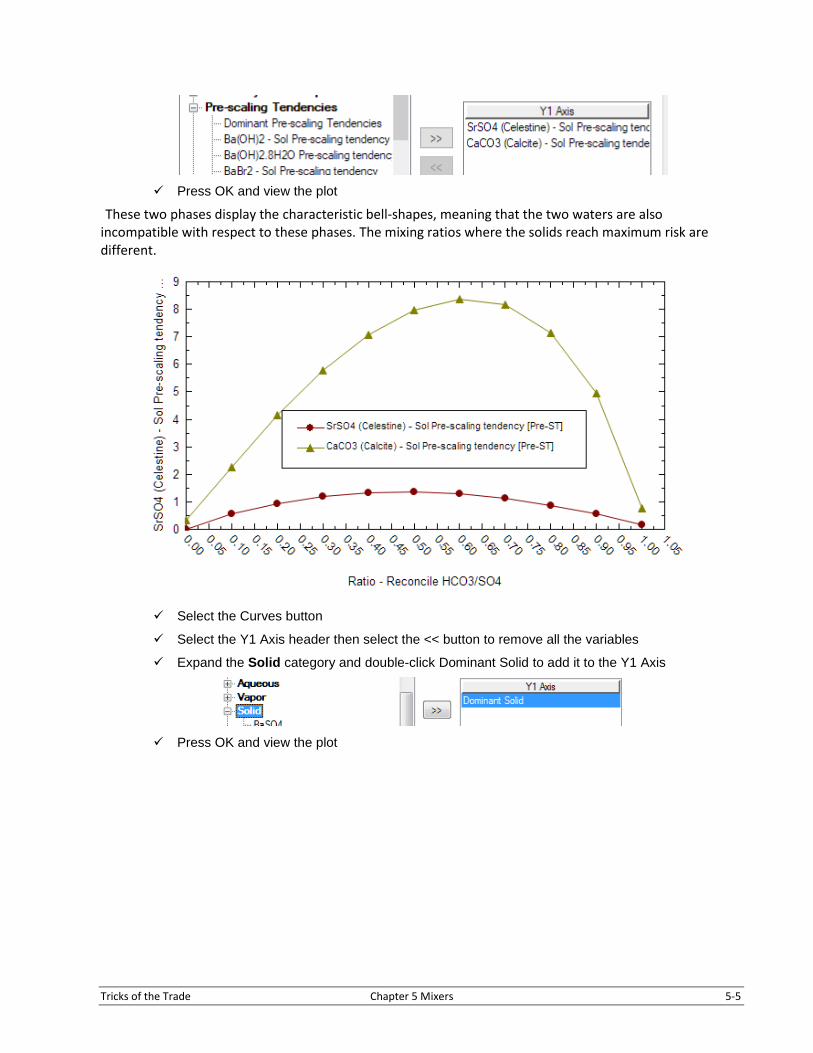
✓ Press OK and view the plot
These two phases display the characteristic bell-shapes, meaning that the two waters are also incompatible with respect to these phases. The mixing ratios where the solids reach maximum risk are different.
✓ Select the Curves button
✓ Select the Y1 Axis header then select the << button to remove all the variables
✓ Expand the Solid category and double-click Dominant Solid to add it to the Y1 Axis
✓ Press OK and view the plot

5-6 Chapter 5 Mixers Tricks of the Trade
The maximum scale mass occurs at 3 different ratios, 5% for BaSO4, 50% for SrSO4, and 75% for CaCO3. The units are in moles, which is useful when looking at absolute values. In this case, however, concentration units will be more useful.
✓ Select the Units Manager button in the toolbar
✓ Select the Customize button
✓ Change the Solids Composition row from Moles to Concentration
✓ Press OK twice to close the Units windows
✓ Refresh the plot by clicking a different tab (for example click on the Definition tab) then click back on the Plot tab

Tricks of the Trade Chapter 5 Mixers 5-7
The curves have similar shapes, but now the high formula weight of BaSO4 makes this curve more pronounced. The ratio where the barite amount is at maximum is at 5% of the High Bicarb/Sulfate stream. We can see this comparing the Ba+2 and SO4
-2 concentrations in their respective waters (view the table below). The amount of Ba+2 and SO4
-2 in the two waters are 0.00109 and 0.0208 moles/kg respectively. They therefore are equivalent in moles, when the High Calcium/Barium water is 19.1 times greater than the High Bicarb/Sulfate water.
Barium and Sulfate concentrations
mg/l Molal Mole Ratio
High Calcium/Barium 150 mg/l Ba+2 0.00109 1
High Bicarb./Sulfate 2000 mg/l SO4-2 0.0208 19.1
Likewise, the calcium to carbonate molar ratio in the two waters is 3.2 moles Ca+2 to 1 mole CO3-2.
Therefore, the maximum mas should occur at 3.2
3.2+1= 76% of the High Bicarb/Sulfate water.
Calcium and Carbonate concentrations
mg/l Molal Mole Ratio
High Calcium/Barium 2000 mg/l Ca+2 0.0499 3.20
High Bicarb./Sulfate 950 mg/l CO3-2 0.0156 1
Lastly, the strontium to sulfate molar ratio is 1 to 6.12, which, of using the same logic would result in
maximum SrSO4 mass forming at 6.12
6.12+1= 86% of the High Calcium/Barium water. However, it instead
occurs at 50% mixture. A question to consider: why does this happen?
Strontium and Sulfate concentrations
mg/l Molal Mole Ratio
High Calcium/Barium 300 mg/l Sr+2 0.0034 1
High Bicarb./Sulfate 200 mg/l SO4-2 0.0208 6.12
✓ Save the file
Summary
This case is an example of how we can test the incompatibility of two waters using the ratio mixing option.

5-8 Chapter 5 Mixers Tricks of the Trade
5.2 Simple Mixer Calculation
Overview
This is a simple two-step calculation. First, we will create two new streams, 0.1 HF and 0.1 CaCl2. We will perform a single point calculation on each. Then, we will mix them in equal amounts. Our goal is to determine the new mixture’s pH.
✓ Select File > New then select File > Save As … and enter ‘Chapter 5’ as the name
1st Stream 2nd Stream
Name 0.1 HF Name 0.1 CaCl2
Unit Set Default Unit Set Default
Names Style Formula Names Set Formula
Framework Aqueous Framework Aqueous
Temperature 30 C Temperature 30 C
Pressure 1 atm Pressure 1 atm
H2O calculated H2O calculated
HF 0.1 mol CaCl2 0.1 mol
✓ Add two new streams with the compositions from the table above
✓ Add a single point, isothermal calculation on each stream
✓ Calculate
The Navigator contians the two streams and their single point calculations. We can now mix the streams.
✓ Highlight the Global Streams icon in the Navigator
✓ Add a new Mixer
✓ Press the <F2> key to rename the mixer ‘HF CaCl2 Mixer’
✓ Select the mixer’s Definition tab

Tricks of the Trade Chapter 5 Mixers 5-9
✓ Highlight 0.1 HF and 0.1 CaCl2 in the Available Streams column
✓ Click the double arrows >> to move them to to the Selected column
✓ Select Single Point Mix as the Mixing Method
✓ Select Isothermal as the Type of Calculation
✓ Press the <F9> key or select the Calculate button
✓ Select the Report tab then scroll down to the
✓ In the Report tab, scroll down to the Stream Parameters section
The pH is 1.44. Does this seem like unusual pH behavior? Mixing an acid and a base should result in a neutralized solution. In this case, the pH is lower than the starting streams.
Mixer Changes
✓ Select the Definition tab

5-10 Chapter 5 Mixers Tricks of the Trade
✓ Change the Mixing Method from Single Point Mix to Multiplier
✓ Click the Specs button
✓ In the Category field, select Variable-Multiplier
✓ Select 0.1 CaCl2 in the Selected Stream field
✓ Select the Survey Range tab
HF CaCl2 Mixer Survey Range
Start 0
End 10
Increment 0.1
✓ Change the survey range according to the table above
✓ Press OK then Calculate
✓ Select the Plot tab then select the Curves button
✓ Press the Y1 Axis header then the << button to remove any variables

Tricks of the Trade Chapter 5 Mixers 5-11
✓ Expand the Additional Stream Parameters category then double click pH Aqueous
✓ Press OK to view the plot
What does this plot indicate about the pH?
✓ Save the file

5-12 Chapter 5 Mixers Tricks of the Trade
5.3 Neutralizing Two Streams In this section, we will learn more about the Volume, Ratio, and Multiplier mixing methods. We will create
two refinery wastewaters, a spent caustic, and a spent sulfuric acid. A third stream will contain air. We will mix the streams and study their speciation.
✓ Create three new streams
✓ Set to formula view or Name view, depending on ease of use
✓ Set all streams to Aqueous Framework
✓ Change the Units Manager based on the settings provided for each stream
5.3 Spent Caustic
Name Spent Caustic
Units Metric Mass Frac
Amount 1000 kg
Temp 50 C
Pressure 1 atm
H2O (mass%) balance
NaOH 0.9
Methyl mercaptan 0.2
NaCl 0.2
H2S 0.5
Phenol 0.2
Naphthenic acid 0.15
NH4Cl 0.07
5.3 Spent Acid
Name Spent Acid
Units Metric, Mass Frac
Amount 1500 kg
Temp 42 C
Pressure 1 atm
H2O (mass%) balance
H2SO4 1.5
Na2SO4 0.5
Na2S2O3 0.3
Lauric acid 5.2
5.3 Air*
Name Air
Units Metric Mole Frac
Amount 3500 mol
Temp 25 C
Pressure 1 atm
H2O (mole%) balance
N2 76.85
O2 20 %
CO2 0.04 %

Tricks of the Trade Chapter 5 Mixers 5-13
✓ Add a new Mixer and rename it ‘Waste Tank’
✓ Add the Spent Caustic and Spent Acid to the Selected field
✓ Select Multplier as the Mixing Method
✓ Click the Specs button
✓ Select Spent Acid as the adjustible stream
✓ Select the Survey Range tab
Multiplier survey range
Start 0
End 1
Increment 0.01
✓ Change the survey range according to the table above
✓ Close the window and Calculate
✓ Select the Plot tab then select the Curves button
✓ Press the Y1 Axis header then the << button to remove any variables
✓ Expand the Additional Stream Parameters category then double click pH Aqueous

5-14 Chapter 5 Mixers Tricks of the Trade
✓ Press OK then view the plot
The steep slope (inflection points) are at about 7.3 pH, 5.1 pH, and 2.9 pH. These pH values are the ends of the buffering regions created by the the the weak acids and bases in the two waters. The pH buffering regions are at the shallow sloped areas.
There are a number of variables to review in a multicomponent mixing calculation like this, and several plots will be studied herein. Remember to clear any variables before proceeding. Click the top double arrow buttons to add or removes curves to or from the X Axis. Click the bottom double arrow buttons to add or remove curves to or from the Y2 Axis.
✓ Change the Names manager so that it displays Formula View -
You will want to toggle among names view as you study the various chemical systems, inorganics are generally easier to interpret in Formula view.
H2S speciation during mixing
✓ Select the Curves button
✓ Change the plot variables to the following
Category Curve Axis
Aqueous HS-1, H2S, S-2 Y1 Axis
Vapor H2S Y1 Axis

Tricks of the Trade Chapter 5 Mixers 5-15
or
✓ Press OK and view the plot
As Spent Acid is added to Spent Caustic, the sulfide speciation shifts to molecular H2S. At about 0.25
Multiplier of the spent acid, an H2S bubble forms as the nearly all the sulfide present in the system is
converted to H2S. This H2S vapor is present until about 0.43 multiplier. The shallow decline of the H2S
vapor is the result of dilution as more liquid is added. Eventually the overall H2S concentration reduces
enough to where the vapor phase collapses under the 1 atm confining pressure.
This can be confirmed by plotting the total dissolved sulfur using concentration units.
✓ Open the Units Manager and select the Customize button.
✓ Set the Aqueous composition to Concentraiton
✓ Open the Variables window. Expand the MBG Totals - Aqueous category
✓ Add S-2 to the Y1 Axis
✓ Remove the H2S Vap from the Y1 Axis
✓ Close the window and view the plot
The updated plot shows all the aqueous concentration

5-16 Chapter 5 Mixers Tricks of the Trade
The amber triangles is the total dissolved sulfide. Its value is 4755 mg/l in the ~1000 L spent caustic that is present in the mixer. As the Spent acid is added, the total dissolved H2S decreases linearly. At 0.25 multiplier, which is about 400 L, there is a sharp concentration drop as H2S partitions to the vapor phase. Eventually sufficient liquid is added at 0.45 multiplier (~650 L) to where the H2S redissolves and continues to decrease in concentration as the total mixer volume increases. Once all the spent acid is added, the final volume is about 2400 L, and so the total dissolved H2S decreases to about 1960 mg/l.
It is also possible to study the results using pH as the x-axis, rather than the Spent Acid Multiplier.
✓ Open the Variables window and change the x-axis to pH
The HS-H2S curves cross at about 6.6 pH. This is the maximum pH-buffering region for the reaction:𝐻𝑆−1 + 𝐻+ = 𝐻2𝑆 (𝑎𝑞).

Tricks of the Trade Chapter 5 Mixers 5-17
The dissolved H2S-aq curve increases steadily from 9 to 6 pH, after which it levels abruptly. This is because any additional H2S that is created as the pH decreases partitions to the vapor phase.
Organic acid speciation during mixing
✓ Select the Curves button and change the plot variables to the following
Category Curve Axis
Additional Stream Parameters pH Aqueous X Axis
Aqueous C12H23O2-1, C12H24O2 Y1 Axis
✓ Press OK and view the plot
Lauric acid (C12H2402 (aq)) – also known by its more formal name dodecanoic acid – comes in with the Spent Acid. As pH decreases, the concentration increases. Note that the crossover occurs at 4.6 pH.
Phenol speciation during mixing
✓ Select the Curves button and change plot variables to the following then press OK
Category Curve Axis
Additional Stream Parameters pH Aqueous X Axis
Aqueous C6H5O-1, C6H5OH Y1 Axis

5-18 Chapter 5 Mixers Tricks of the Trade
The phenol-phenolate crossover occurs at a high pH of 9.39. Thus, as the spent acid mixes with the spent caustic, this reaction will create the buffering at high pH.
Methyl mercaptan speciation during mixing
✓ Select the Curves button and change plot variables to the following then press OK
Category Curve Axis
Additional Stream Parameters pH Aqueous X Axis
Aqueous CH3S-1, CH4S Y1 Axis
Vapor CH4S Y1 Axis

Tricks of the Trade Chapter 5 Mixers 5-19
The Mercaptan reaction 𝐶𝐻3𝑆−1 + 𝐻+ = 𝐶𝐻3𝑆𝐻 (𝑎𝑞) also occurs at a high pH of 10. This will be the first H+ adsorption reaction that occurs when the spent acid mixes. These curves cross at different pH levels. The crossing points are called equivalence points and are where buffering is the greatest.
Next Step – H2S Safety
The next step in this case is to review the H2S aqueous-vapor partitioning. The existence of an H2S vapor below 6 pH is a safety hazard. Therefore, the properties of the mixture will be investigated further. The first calculation will be to determine the vapor pressure of the mixture. The confining pressure is 1 atm, the default value. Now however, the software will compute what the confining pressure needs to be so that no vapor forms
Pressurized system
The first calculation is consisten with what is already computed, except in this next step the vapor pressure of the mix will be computed.
✓ Select the Definitions tab
✓ Change the Type of Calculation to Bubble Point
✓ Change the Calculate cell from Temperture to Pressure
✓ Calculate
✓ Plot the Total pressure (Stream Parameters category) on the Y1 axis against either the pH, which is the default, or gains the Waste Acid multiplier (Survey Variables)
The resulting plots show that the maximum confining pressure is about 1.1 atm. At 5.5 pH or at about 0.28 multiplier (~400 l) the H2S vapor pressure reaches a maximum. Thus, according to this calculation, the mixing tank will need to be closed with at least a 1.2 atm positive pressure to eliminate degassing.

5-20 Chapter 5 Mixers Tricks of the Trade
Or
Case 2 – Atmospheric system
The purpose of this example is to estimate the amount of H2S in the nearby air if the tank is open to the atmosphere. The Air stream amount is 3500 moles. This occupies a volume of 85.6 m3. This is an arbitrary value, and represents the airspace 5 m high above a tank with a radius of 2.3 m.
✓ Return to the Definitions tab
✓ Start by editing the units – Change the Vapor Composition from moles to mole fraction
✓ Next, change the Mole fraction units from mole % to ppm (mole)
✓ Add Air to add it to the Selected column

Tricks of the Trade Chapter 5 Mixers 5-21
✓ Change the Type of Calculation back to Isothermal
✓ Calculate
✓ Select the Plot tab and change the plot varialbes
o Change the x-axis to Multiplier – Spent Acid (Survey Variables category)
o Change the y1 axis to H2S – vapor
✓ Press Ok and view the plot
Air, or a headspace, is now present in all mixing points, and not only when H2S form the headspace. As a
result, H2S is in the air and the fraction increases as the Spent acid amount increases. it reaches a
maximum value of ~38000 ppmV at the 0.25 multiplier and remains relatively constant thereafter. Thus
virtually any mixture of these two waste stream when open to the atmosphere will present an H2S safety
hazard.

5-22 Chapter 5 Mixers Tricks of the Trade
Summary
The mixing results are secondary to the objective of comparing the different mixing scenarios. The list below summarizes the mix types.
Multiplier Survey – This survey calculation adjusts the inflow mass of the selected stream only. Its mass is multiplied by the multiplier value.
𝑆𝑡𝑟𝑒𝑎𝑚 𝑀𝑎𝑠𝑠 ∗ 𝑀𝑢𝑙𝑡𝑖𝑝𝑙𝑖𝑒𝑟 = 𝑇𝑜𝑡𝑎𝑙 𝐼𝑛𝑓𝑙𝑜𝑤 𝑀𝑎𝑠𝑠
The second (third, fourth, etc.) stream inflows are kept constant.
Volume Survey – This survey calculation adjusts the inflow volume while keeping the other stream volumes constant.
Ratio Survey – The Ratio survey calculation adjusts both inflow streams using the following rule
𝑆𝑒𝑙𝑒𝑐𝑡𝑒𝑑 𝑆𝑡𝑟𝑒𝑎𝑚 𝑀𝑎𝑠𝑠 ∗ 𝑅𝑎𝑡𝑖𝑜 = 𝐼𝑛𝑓𝑙𝑜𝑤 𝑀𝑎𝑠𝑠
𝑆𝑢𝑚 𝑜𝑓 𝑂𝑡ℎ𝑒𝑟 𝑆𝑡𝑟𝑒𝑎𝑚 𝑀𝑎𝑠𝑠𝑒𝑠 ∗ (1 − 𝑅𝑎𝑡𝑖𝑜) = 𝑂𝑡ℎ𝑒𝑟 𝑀𝑎𝑠𝑠
In this survey calculation, the overall inflow mass is kept constant.

Tricks of the Trade Chapter 5 Mixers 5-23
5.4 Creating a Titration Curve
Overview
A titration curve shows the mixing of two reagents, typically an acid and base. The software can mix two or more reagent streams and model typical acid-base or other potentiometric titrations. In this example, we will titrate seawater down to 4.5 pH to compute its alkalinity.
Getting started
Adding the seawater analysis
There are several Seawater objects installed with the software. They are found in the Object library with several other standard streams. So, instead of starting from a laboratory analysis, you will add the Seawater object from the library to the Navigator pane.
✓ Open the Object Library if it is not opened at the right of the screen–
o Click on View-Toolbars-Object Library (from the menu)
✓ Drag the Standard Seawater Analysis object to the Navigator Panel
Seawater is at the bottom of the Object Library. When you drag it to the Navigator panel, drag to the top-most Streams or to below the last object in the panel.
✓ Add a Reconciliation object and name it Reconciled Seawater
✓ Calculate

5-24 Chapter 5 Mixers Tricks of the Trade
Adding the 1N H2SO4 reagent
✓ Add a new stream and give it a name, 1 N H2SO4 (1ml) -
✓ Change the units to Metric-Batch-Molar Conc
✓ Change the Stream amount to 0.001 L (1ml)
✓ Add H2SO4 to the grid and enter a value of 0.5 mol/l
Adding the titration apparatus
✓ Add a new Mixer and rename it ‘Titration Apparatus’
✓ Add the Reconciled Seawater and 1N H2SO4 to the Selected section
✓ Select Multiplier as the Mixing Method
✓ Open the Specs button and 1N H2SO4 as the Adjusted stream
✓ Set the Survey: Start at 0, end at 10 (ml) with increments of 0.1 (ml).
✓ Calculate
✓ Cick on the Plot tab and plot the pH in the Y1 axis

Tricks of the Trade Chapter 5 Mixers 5-25
The resulting pH titration curve is the standard approach for measuring total alkalinity. The alkalinity endpoint is 4.5 pH, and the corresponding H2SO4 multiplier is 2.8, or 2.8 ml.
The conversion from ml H2SO4 to mg/l Alkalinity as HCO3 is straight forward:
𝐴𝑙𝑘𝑎𝑙𝑖𝑛𝑖𝑡𝑦 𝑎𝑠 𝐻𝐶𝑂3−1 (
𝑚𝑔
𝑙) =
𝑣𝑜𝑙 𝐻2𝑆𝑂4 (𝑚𝑙) ∗ 𝑁 𝐻2𝑆𝑂4 (𝑒𝑞𝑙
)
𝑣𝑜𝑙 𝑆𝑎𝑚𝑝𝑙𝑒 (𝑚𝑙)⁄ ∗ 61000 (
𝑚𝑔
𝑒𝑞)
𝐴𝑙𝑘𝑎𝑙𝑖𝑛𝑖𝑡𝑦 𝑎𝑠 𝐻𝐶𝑂3−1 (
𝑚𝑔
𝑙) =
2.8 (𝑚𝑙) ∗ 1 (𝑒𝑞𝑙
)
1000 (𝑚𝑙)⁄ ∗ 61000 (
𝑚𝑔
𝑒𝑞) = 170.8
𝑚𝑔
𝑙𝑎𝑠 𝐻𝐶𝑂3
−1