Mixed Inductive-Coinductive Reasoning
340
Mixed Inductive-Coinductive Reasoning Types, Programs and Logic Proefschriſt ter verkrijging van de graad van doctor aan de Radboud Universiteit Nijmegen op gezag van de rector magnificus prof. dr. J.H.J.M van Krieken, volgens besluit van het college van decanen in het openbaar te verdedigen op donderdag 19 april 2018 om 16:30 uur precies door Henning Basold geboren op 16 juni 1986 te Braunschweig (Duitsland)
Transcript of Mixed Inductive-Coinductive Reasoning

Mixed Inductive-Coinductive ReasoningTypes, Programs and Logic
Proefschriftter verkrijging van de graad van doctoraan de Radboud Universiteit Nijmegen
op gezag van de rector magnificus prof. dr. J.H.J.M van Krieken,volgens besluit van het college van decanen
in het openbaar te verdedigen op donderdag 19 april 2018om 16:30 uur precies
door
Henning Basold
geboren op 16 juni 1986te Braunschweig (Duitsland)

PromotorenProf. dr. Jan RuttenProf. dr. Herman Geuvers
CopromotorDr. Helle Hvid Hansen (Technische Universiteit Delft)
ManuscriptcommissieProf. dr. Bart Jacobs (Voorzitter)Prof. dr. Neil Ghani (University of Strathclyde, Verenigd Koninkrijk)Prof. dr. Tarmo Uustalu (Tallinn University of Technology, Estland)Dr. Andreas Abel (Chalmers University of Technology en Götenborgs
Universitet, Zweden)Dr. Ekaterina Komendantskaya (Heriot-Watt University, Verenigd Koninkrijk)
This research has been carried out under the auspices of the iCIS (institute for Computing andInformation Science) of the Radboud University Nijmegen, the Formal Methods Group of the CWI,and the research school IPA (Institute for Programming research and Algorithmics).
This research has been supported by NWO (grant number 612.001.021).
cba Copyright © 2018 Henning Basold, under a Creative Commons Attribution-ShareAlike 4.0International License: http://creativecommons.org/licenses/by-sa/4.0/.
ISBN 978-0-244-67206-5Typeset with XƎLATEXPrinted and published by Lulu
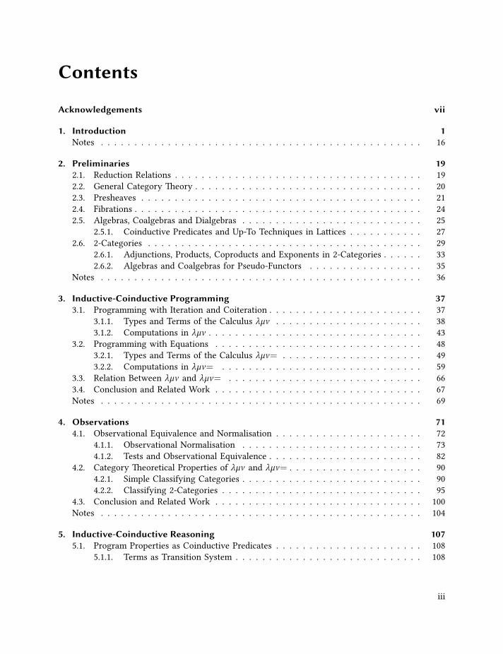
Contents
Acknowledgements vii
1. Introduction 1Notes . . . . . . . . . . . . . . . . . . . . . . . . . . . . . . . . . . . . . . . . . . . . . . . . 16
2. Preliminaries 192.1. Reduction Relations . . . . . . . . . . . . . . . . . . . . . . . . . . . . . . . . . . . . . 192.2. General Category Theory . . . . . . . . . . . . . . . . . . . . . . . . . . . . . . . . . . 202.3. Presheaves . . . . . . . . . . . . . . . . . . . . . . . . . . . . . . . . . . . . . . . . . . 212.4. Fibrations . . . . . . . . . . . . . . . . . . . . . . . . . . . . . . . . . . . . . . . . . . . 242.5. Algebras, Coalgebras and Dialgebras . . . . . . . . . . . . . . . . . . . . . . . . . . . 25
2.5.1. Coinductive Predicates and Up-To Techniques in Lattices . . . . . . . . . . . 272.6. 2-Categories . . . . . . . . . . . . . . . . . . . . . . . . . . . . . . . . . . . . . . . . . 29
2.6.1. Adjunctions, Products, Coproducts and Exponents in 2-Categories . . . . . . 332.6.2. Algebras and Coalgebras for Pseudo-Functors . . . . . . . . . . . . . . . . . 35
Notes . . . . . . . . . . . . . . . . . . . . . . . . . . . . . . . . . . . . . . . . . . . . . . . . 36
3. Inductive-Coinductive Programming 373.1. Programming with Iteration and Coiteration . . . . . . . . . . . . . . . . . . . . . . . 37
3.1.1. Types and Terms of the Calculus λµν . . . . . . . . . . . . . . . . . . . . . . 383.1.2. Computations in λµν . . . . . . . . . . . . . . . . . . . . . . . . . . . . . . . . 43
3.2. Programming with Equations . . . . . . . . . . . . . . . . . . . . . . . . . . . . . . . 483.2.1. Types and Terms of the Calculus λµν= . . . . . . . . . . . . . . . . . . . . . 493.2.2. Computations in λµν= . . . . . . . . . . . . . . . . . . . . . . . . . . . . . . 59
3.3. Relation Between λµν and λµν= . . . . . . . . . . . . . . . . . . . . . . . . . . . . . 663.4. Conclusion and Related Work . . . . . . . . . . . . . . . . . . . . . . . . . . . . . . . 67Notes . . . . . . . . . . . . . . . . . . . . . . . . . . . . . . . . . . . . . . . . . . . . . . . . 69
4. Observations 714.1. Observational Equivalence and Normalisation . . . . . . . . . . . . . . . . . . . . . . 72
4.1.1. Observational Normalisation . . . . . . . . . . . . . . . . . . . . . . . . . . . 734.1.2. Tests and Observational Equivalence . . . . . . . . . . . . . . . . . . . . . . . 82
4.2. Category Theoretical Properties of λµν and λµν= . . . . . . . . . . . . . . . . . . . . 904.2.1. Simple Classifying Categories . . . . . . . . . . . . . . . . . . . . . . . . . . . 904.2.2. Classifying 2-Categories . . . . . . . . . . . . . . . . . . . . . . . . . . . . . . 95
4.3. Conclusion and Related Work . . . . . . . . . . . . . . . . . . . . . . . . . . . . . . . 100Notes . . . . . . . . . . . . . . . . . . . . . . . . . . . . . . . . . . . . . . . . . . . . . . . . 104
5. Inductive-Coinductive Reasoning 1075.1. Program Properties as Coinductive Predicates . . . . . . . . . . . . . . . . . . . . . . 108
5.1.1. Terms as Transition System . . . . . . . . . . . . . . . . . . . . . . . . . . . . 108
iii
Contents
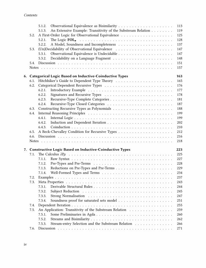
5.1.2. Observational Equivalence as Bisimilarity . . . . . . . . . . . . . . . . . . . . 1135.1.3. An Extensive Example: Transitivity of the Substream Relation . . . . . . . . 119
5.2. A First-Order Logic for Observational Equivalence . . . . . . . . . . . . . . . . . . . 1255.2.1. The Logic FOL . . . . . . . . . . . . . . . . . . . . . . . . . . . . . . . . . . 1285.2.2. A Model, Soundness and Incompleteness . . . . . . . . . . . . . . . . . . . . 137
5.3. (Un)Decidability of Observational Equivalence . . . . . . . . . . . . . . . . . . . . . 1475.3.1. Observational Equivalence is Undecidable . . . . . . . . . . . . . . . . . . . . 1475.3.2. Decidability on a Language Fragment . . . . . . . . . . . . . . . . . . . . . . 148
5.4. Discussion . . . . . . . . . . . . . . . . . . . . . . . . . . . . . . . . . . . . . . . . . . 151Notes . . . . . . . . . . . . . . . . . . . . . . . . . . . . . . . . . . . . . . . . . . . . . . . . 157
6. Categorical Logic Based on Inductive-Coinductive Types 1636.1. Hitchhiker’s Guide to Dependent Type Theory . . . . . . . . . . . . . . . . . . . . . 1656.2. Categorical Dependent Recursive Types . . . . . . . . . . . . . . . . . . . . . . . . . 176
6.2.1. Introductory Example . . . . . . . . . . . . . . . . . . . . . . . . . . . . . . . 1776.2.2. Signatures and Recursive Types . . . . . . . . . . . . . . . . . . . . . . . . . 1786.2.3. Recursive-Type Complete Categories . . . . . . . . . . . . . . . . . . . . . . . 1816.2.4. Recursive-Type Closed Categories . . . . . . . . . . . . . . . . . . . . . . . . 187
6.3. Constructing Recursive Types as Polynomials . . . . . . . . . . . . . . . . . . . . . . 1886.4. Internal Reasoning Principles . . . . . . . . . . . . . . . . . . . . . . . . . . . . . . . 199
6.4.1. Internal Logic . . . . . . . . . . . . . . . . . . . . . . . . . . . . . . . . . . . . 1996.4.2. Induction and Dependent Iteration . . . . . . . . . . . . . . . . . . . . . . . . 2026.4.3. Coinduction . . . . . . . . . . . . . . . . . . . . . . . . . . . . . . . . . . . . . 210
6.5. A Beck-Chevalley Condition for Recursive Types . . . . . . . . . . . . . . . . . . . . 2126.6. Discussion . . . . . . . . . . . . . . . . . . . . . . . . . . . . . . . . . . . . . . . . . . 216Notes . . . . . . . . . . . . . . . . . . . . . . . . . . . . . . . . . . . . . . . . . . . . . . . . 218
7. Constructive Logic Based on Inductive-Coinductive Types 2237.1. The Calculus λPµ . . . . . . . . . . . . . . . . . . . . . . . . . . . . . . . . . . . . . . 225
7.1.1. Raw Syntax . . . . . . . . . . . . . . . . . . . . . . . . . . . . . . . . . . . . . 2277.1.2. Pre-Types and Pre-Terms . . . . . . . . . . . . . . . . . . . . . . . . . . . . . 2287.1.3. Reductions on Pre-Types and Pre-Terms . . . . . . . . . . . . . . . . . . . . . 2297.1.4. Well-Formed Types and Terms . . . . . . . . . . . . . . . . . . . . . . . . . . 234
7.2. Examples . . . . . . . . . . . . . . . . . . . . . . . . . . . . . . . . . . . . . . . . . . . 2377.3. Meta Properties . . . . . . . . . . . . . . . . . . . . . . . . . . . . . . . . . . . . . . . 243
7.3.1. Derivable Structural Rules . . . . . . . . . . . . . . . . . . . . . . . . . . . . . 2447.3.2. Subject Reduction . . . . . . . . . . . . . . . . . . . . . . . . . . . . . . . . . 2457.3.3. Strong Normalisation . . . . . . . . . . . . . . . . . . . . . . . . . . . . . . . 2477.3.4. Soundness proof for saturated sets model . . . . . . . . . . . . . . . . . . . . 251
7.4. Dependent Iteration . . . . . . . . . . . . . . . . . . . . . . . . . . . . . . . . . . . . . 2557.5. An Application: Transitivity of the Substream Relation . . . . . . . . . . . . . . . . 259
7.5.1. Some Preliminaries in Agda . . . . . . . . . . . . . . . . . . . . . . . . . . . . 2607.5.2. Streams and Bisimilarity . . . . . . . . . . . . . . . . . . . . . . . . . . . . . . 2627.5.3. Stream-entry Selection and the Substream Relation . . . . . . . . . . . . . . 266
7.6. Discussion . . . . . . . . . . . . . . . . . . . . . . . . . . . . . . . . . . . . . . . . . . 271
iv

Contents
Notes . . . . . . . . . . . . . . . . . . . . . . . . . . . . . . . . . . . . . . . . . . . . . . . . 273
8. Epilogue 277
References 279Own Publications . . . . . . . . . . . . . . . . . . . . . . . . . . . . . . . . . . . . . . . . . 299
Subject Index 301
Notation Index 305
A. Confluence for λµν= 309
B. Proofs of Section 6.3 315
Summary 319
Samenvatting 321
Zusammenfassung 323
Curriculum Vitae 327
v


Acknowledgements
Ich sage: laßt alle Hoffnung fahren, ihr, die ihr in die Beobachtung eintretet.(Eng.: I say, abandon all hope, you who enter the realm of observation.)
— Galileo Galilei in Bertolt Brechts “Leben des Galilei”, Akt 9.
Before we start with the technical content of the thesis, I would like to thank a few people thatcontributed to its development in one way or another.
First and foremost, I would like to thank my supervisor Helle Hvid Hansen. Her infinite patience,her vast knowledge of scientific topics and the English language, and her attention to detail mademe not only a better researcher but also a much better writer. Before I started my PhD, I didan internship at the CWI in Amsterdam with Marcello Bonsangue and Jan Rutten, who then alsobecame my promoter. It was there that I met Helle the first time and we started to have scientificand non-scientific conversations. We also shared good evenings outside of work, through whichI learned about very nice restaurants in Amsterdam, and one or two tricks in the kitchen. Bothour discussions and Helle’s incredibly detailed feedback improved my research, mathematical andwriting skills tremendously, and without them, my thesis would be far worse than it is now.
As I already mentioned, I did an internship with Jan before he became my promoter. Alreadyat that time it became clear that Jan finds a good balance between giving one a lot of freedomand guidance. But not just that, Jan has also the ability, which amazes me every time, to makesuggestions that open up new paths or lead to vast simplifications. This impression proved to beright, and I am greatly indebted to Jan in his role as my supervisor. Without him, I would haveneither arrived at the research topics of my thesis nor at all where I am today. His constant support,his suggestions, feedback and his ability to listen are invaluable.
Last but not least, Herman Geuvers entered the team when my research shifted towards typetheory. I learned a lot from Herman about logic and type theory. He has an enormous knowledgeabout these fields, and I could always come by and get an extensive answer. If the answer wouldbe too complicated to be answered on the spot, he would go to his cabinet or bookshelf and takea printed publication, sometimes his own, that would answer the question. Indeed, the strongnormalisation proof in the last chapter would not be there, had he not given me his ’94 paper onstrong normalisation of the calculus of constructions. Making a long story short, Herman is anothercornerstone in my development as a researcher, and I would like to wholeheartedly thank him foreverything he did and the positive atmosphere he creates.
Overall, I am equally indebted to all of you, Helle, Jan and Herman, for your support, yourkindness and what you have taught me. You were the best team of supervisors that I could envision!
I would like to thank other people that have directly contributed to the content of this thesis.First, there is the reading committee consisting of Andreas Abel, Neil Ghani, Bart Jacobs, EkaterinaKomendantskaya and Tarmo Uustalu. I am grateful for all the time and effort they put into reviewingthis, fairly lengthy, thesis and all the suggestions they made. In particular, I am happy that afundamental flaw was found by Andreas before publication.
Next, there are all the people that I have collaborated with on publications: Damien, Helle, HenningG., Herman, Jan, Jean-Éric, Jurriaan, Katya, Marcello, Michaela, Niels and Stefan. I would like tothank all of them for being fantastic collaborators.
vii

Acknowledgements
Finally, there are a few other people that I would like to mention because they had a directinfluence on the content and even the existence of this thesis. I am especially indebted to StefanMilius, who brought me into contact with Jan and thus opened up the path to my PhD. Thisresulted in an internship with Jan and Marcello. During this internship and afterwards, I had someoutstanding discussions with Marcello, which resulted in my first publication. I am grateful forMarcello’s scientific guidance, which laid the foundations for my later work in theoretical computerscience, particularly in the field of coalgebra.
Science demands a certain amount of dedication, a demand that can be very high at times andone that can only be fulfilled if we have people of support and collaboration around us. It is thesepeople that I would like to dedicate the opening quote to. Brecht derived it from the inscription“Abandon all hope, ye who enter here.” above the entrance to hell in Dante Alighieri’s La DivinaCommedia. The phrase is used by Galilei in Brecht’s play when he picks up again his studies on therotation of the sun and describes his approach to science: Work slowly, question everything, repeatexperiments and compare the outcomes, distrust everything that fits your beliefs, and only accept aresult if all other possibilities can be excluded. This is a daunting task, which can not only be lonelyat times but also carries the danger of becoming ignorant of the surrounding world. However, I wasvery lucky and met some fantastic people along the way, who reminded me about what is importantin life and who were willing to share this daunting task. I mentioned my scientific collaboratorsand guides already above, but there are further important people in my life.
In particular, I would like to thank Pauline Chew, Simone Lederer and Jurriaan Rot. Pauline wasalways around with continuous support and for, often intense, conversations over food or late atnight. Thank you, Pauline, for all this and, above all, for making me grow as a person. With SimoneI had a perfect travel partner, who was always up for spontaneous activities in the weekend andfor good conversations. To you also a big thank you, Simone, for the good time and the differentperspectives you offered. And, I would like to thank you both, Pauline and Simone, for beingmy paranimphs. I met Jurriaan at the CWI, from where we became friends and research partners.Among the many interests that we share, our running sessions and bike rides, cooking and, of course,coalgebras are the most important ones to me. Thank you, Jurriaan, for all the good cooperation,and for your help with my thesis and articles.
The next shout goes out to my friends in Nijmegen, with whom I spent a great deal of my sparetime, be it at dinners, watching films, going to concerts or to museums: Alexis, Dario, Elena, Gabriel,Jacopo, Joshua, Michael, Michele, Pauline, Robbert, Rui Fei, Simon, Sjef, Steffen and Tim, and myflatmate Katja. Some friends I also found in Amsterdam, like Nick, who was my flatmate for twoyears, and with whom I shared meals and good conversations in the evenings. Sung is another greatperson that I met at the CWI. We had many discussions about Reo and life in general. Thank youall for the pleasant time I had in the Netherlands, each of you knows what we share.
Among the fantastic people I met, there are also those that I am lucky to have or have had ascolleagues. My first job was the civil service in the hospital in Braunschweig, where I found inThomas Joosten and Jürgen Feß people, who supported me in my choice to study but also made meaware of possible pitfalls. I am thankful that I could work before and during my studies with UdoHanfland and the people at BBR in Braunschweig, where I learned a lot about programming, projectmanagement and collaboration.
At the university in Braunschweig, I am indebted to Jiří Adámek, Michaela Huhn and Stefan Miliusfor their supervision of my master’s thesis. Also, I would like to thank Rainer Löwen for his lectures,
viii
which shaped my mathematical mind, and Fiona Gottschalk, Nadine Hattwig, Sebastian Struckmannand Kristof Teichel for the good time we had racking our brains over (algebraic) topology.
The next stage was my time at the CWI, where I met many great people. The first was probablyAlexandra Silva. I owe her a lot, as she brought me in contact with Nick, gave us some basic furnitureand later often provided me with shelter in Nijmegen (thanks also to Neko for being such a goodhost!). Besides being an excellent cook, Alexandra was a good friend and colleague in Nijmegen. AtCWI, I also got in contact with Matteo Mio with whom I have, on and off, good discussions aboutmathematics, logic, geeky topics but also some nice evenings out. Also Enric Cosme-Llópez wasover at CWI as visitor and we had, both, in Amsterdam and in Lyon, a few good evenings. Sincewe are at it, I would like to thank also all the other people that I met at CWI: Dominik, Erik, Farhad(especially for the stories and film recommendations!), Frank (for the jokes and famous FM dinners),Joost, Julian, Kasper, Michiel, Nikos, Stijn and Vlad.
At the Radboud University itself, I crossed paths with many people that I would like to thankas well. One part of working at the university is teaching. I was lucky enough to assist in thecombinatorics course given by Engelbert, who is a fabulous teacher and prepares everything someticulously that there is nothing more that an assistant could wish for. Another part of working atthe university is research and writing. I would like to thank Bart for his scientific and initial financialsupport, for his feedback and for managing the reading committee of my thesis. The last part ofworking is, of course, the environment. I am grateful for all the people at the Radboud university thatmade working there a pleasant experience: Aleks, Arjen, Baris, Bart, Bas S., Bas W., Bram, Camille,Dan, Elena M., Elena S., Engelbert, Erik, Fabian, Fabio, Freek, Frits, Gabriel, Guillaume, Hans, Henk,Herman, Ingrid, Irma, Jacopo, Jonce, Josef, Joshua, Jurriaan, Kasper, Kenta, Maaike, Markus, Mathys,Matteo S., Max, Maya, Michael, Michiel, Mohsen, Nicole, Niels, Paul, Perry, Peter, Ralf, Rick, Ridho,Robbert, Robert, Robin, Ronny, Ruifei, Saskia, Simone L., Simone M., Suzan, Tim, Tom C., Tom H.,Twan, Zaheer. In particular, I would like to thank the Data Science group that I could still feel beinga part of, even though I was technically in another group after the reorganisation.
And then there are the people that I met “in the wild”, that is, at conferences, workshops or otheroccasions. I am happy to be part of the coalgebra and TYPES community and would like to thankthem for their very warm and welcoming atmosphere. Apart from the people that I have mentionedalready, I would like to especially thank Andreas for our discussions that led me to the topics of thelast two chapters; Clemens for hosting me in Edinburgh and for being a friend in general; Filippofor being a great roommate on Barbados and for initialising my contact to work in Lyon; Katya forour discussions and her invitations to Scotland; Neil for our joint workshop and his insights intocategory theory; Prakash for bringing together researchers through workshops and SIGLOG; Tarmofor my fantastic first experience of TYPES in Tallinn and our discussions; and finally Daniela forbeing a perfect flatmate and friend, who gave me also many scientific insights.
I want to end by coming back to my roots in Braunschweig, where I was happy to have foundsome very good friends: Anja, Christoph, Christian, Lea & Patrick and Philipp & Kathrin. Thankyou all for your friendship and the great time we spent together. I would also like to express mygratitude in memory to Rudolf, Anselm, Inge, Helga & Alfred. And finally, I would like to thank myfamily, my parents and Virginie for their support and love.
Henning Basold, February 2018, Lyon.
ix


CHAPTER 1
Introduction
Thought must never submit, neither to a dogma, nor to a party, nor to a passion, nor to an interest, nor to apreconceived idea, nor to whatever it may be, save to the facts themselves, because, for thought, submissionwould mean ceasing to be.
— Henri Poincaré, 1909.1
The purpose of this thesis is to systematically study languages for specifying and reasoning aboutmixed inductive-coinductive structures and processes. We will focus mostly on type theoretic andcategory theoretic languages, but some of the reasoning principles are based on standard bisimula-tions and up-to techniques. In the course of this thesis, we will analyse existing simple type theoriesthat allow the specification of inductive-coinductive processes, and we will exhibit several reasoningprinciples for these type theories: through category theory, by using coinductive predicates and rela-tions combined with up-to techniques, in form of a logic, and in certain cases by automatic decisionprocedures. Moreover, we will develop a dependent type theory, both category theoretically and asa syntactic calculus, that is based solely on inductive-coinductive types. As we will see, this typetheory can serve as a framework for quite general inductive-coinductive definitions and proofs, andforms the pinnacle in expressivity of this thesis.
In the remainder of this introduction, we will motivate the study of inductive-coinductive reasoningand provide an overview of the developments that happen throughout this thesis. To illustrate why itis important to study inductive-coinductive reasoning in its own right, we will first discuss an exampleof an inductive-coinductive property that pervades this thesis and that illustrates beautifully howinductive-coinductive reasoning arises naturally in Mathematics and Computer Science. Afterwards,we will give a brief historical overview, discuss the problems that will be tackled in this thesisand detail the approach that we take. We will finish the introduction with a discussion of thecontributions and outline of this thesis.
Background and MotivationAre you sitting comfortably? Then let us dive into the story of mixed induction-coinduction andhow it can help us in the practice of Mathematics and Computer Science.
Induction and coinduction are threads that cross the landscape of Mathematics and ComputerScience as methods to define objects and reason about them. Of these two, induction is by far thebetter known technique, although disguised coinduction has always been around. It was only inrecent years that we began to see through this disguise and developed coinduction as a technique inits own right. This led to some remarkable theory under the umbrella of coalgebra and to strikingapplications of coinduction.
One of the topics in coalgebra that is actively researched are so-called behavioural differentialequations (BDE) [Rut03; Rut05], which allow for very concise and intuitive process specifications,analogous to the differential equations from Mathematical Analysis. However, BDEs also inherit
1

Chapter 1. Introduction
from their analytic counterpart the problem that a system of equations may specify impossiblebehaviour, and therefore may not have a unique solution or may have no solution at all. Thestarting point of the research, which led up to this thesis, was thus to extend the known formatsfor BDEs to cover wider application areas, while guaranteeing that the specified behaviour in thesemore general formats is still well-defined. Once we have the ability to specify processes, it isnatural to also investigate reasoning principles for such processes to, for example, to be able tocompare their behaviour. Generalising process specifications and exhibiting reasoning principles forthese processes were the two main goals of the NWO project “Behavioural Differential Equations”(612.001.021), in which part of the research for this thesis has been conducted. So how does mixedinduction-coinduction fit into this agenda?
As it turns out, induction and coinduction are complementary techniques, they are dual in aprecise sense that we will discuss later. Being complementary, it is often necessary to use bothtechniques or even intertwine them. The combination of induction and coinduction allows us, forinstance, to construe forms of behavioural differential equations whose expressiveness exceeds thatof the currently available forms. We will also see that combined induction-coinduction is oftenused implicitly, just like induction and coinduction used to be. Thus, the purpose of this thesis isto systematically study the combination of induction and coinduction, which I hope, if anything,inspires others to work on and use inductive-coinductive techniques.
The perspective that we will take in this thesis is that of logic and computation. However, thisshould not limit the applicability of the results presented in this thesis to Computer Science. Rather,the logics developed here are largely independent of the field, as are many of the ideas. I think thatmany objects that occur in Mathematics, Computer Science, and other branches of science, in whichwe build formal models, lend themselves to a mixed inductive-coinductive description. Therefore, Iwish to demonstrate, besides presenting general theory, also the use of inductive-coinductive objectsin an accessible way. That being said, some parts of this thesis presuppose knowledge of categorytheory (Section 4.2 and Chapter 6) and an understanding of dependent type theory (Chapter 6and Chapter 7). To support a reader unfamiliar with any of these, we provide in Section 6.1 ashort introduction to dependent type theory, and introduce some notations and non-standard bitsof category theory in Chapter 2. Despite these requirements, I hope that the reader may still findpleasure in reading this thesis, and may obtain new insights from examples like that in Section 7.5.
Induction and CoinductionSo what are induction and coinduction? And how can their combination contribute to our under-standing of problems in Mathematics and Computer Science and help solving these problems? Theway we will approach these questions is through the slogan that2
inductive objects describe terminating computations and values, whereascoinductive objects describe the behaviour of observable processes.
Consider, for instance, natural numbers and infinite sequences, from here on called streams, ofnatural numbers. The former illustrate the idea of terminating computations that result in values:every computation on natural numbers terminates in either zero or the successor of another naturalnumber. For instance, the number “1” is a value, since it is the successor of zero, whereas “1 + 2”is not a value but it computes to the value “3”. Streams of natural numbers, on the other hand, are
2

observable processes. To illustrate this, let us picture a box with a screen labelled “head” that displaysa natural number and a button labelled “tail”. If we push the button “tail”, the state of the box maychange and a new number may be displayed on the box. We can observe the behaviour of the box byrepeatedly pushing the “tail” button and noting down all the numbers that we see, thereby obtainingan arbitrarily long sequence of numbers. This is illustrated in the following diagram, where eachsquare represents the unknown state of the box, the double arrows labelled “head” point to thedisplayed values, and “tail”-labelled arrows signify state changes through button pushes.
n0
head
tail
n1
head
tail
n2
head
tail
n3
head…
In fact, we can use these descriptions to characterise natural numbers and streams as follows.First of all, for a given type3 X , we will write x : X if x is an element of type X . Let N be atype of natural numbers and Nω a type of streams over natural numbers, both of which we willcharacterise now without further specifying their internal structure.4 We have already said that thenatural numbers are characterised by having an element zero and a successor map, that is, thereis an element 0 : N and a map suc : N → N. In contrast to this, the streams come with two mapshd : Nω → N and tl : Nω → Nω that allow us to obtain the head and the tail of a stream. Note thatthe structure on N allows us to construct elements of N, hence we will refer to 0 and suc generallyas constructors. Streams have the dual property, their structure is determined by maps out of Nω ,the observations hd and tl that we can make on streams. Suppose now that X is a type that comeswith a distinguished element x0 : X and a map s : X → X . We will compactly denote this as a triple(X ,x0, s) and call it an algebra. What makes N special among such algebras is that there is a uniquemap f : N→ X , such that, for all n : N,
f (0) = x0 and f (suc(n)) = s(f (n)). (1.1)
This is summed up by saying that (N, 0, suc) is initial among all algebras (X ,x0 : X , s : X → X ).Dually, streams are characterised by the property that (Nω , hd, tl) is final among all coalgebras(Y ,h : Y → N, t : Y → Y ), which means that there is a unique map д : Y → Nω such that, for ally : Y
hd(д(y)) = h(y) and tl(д(y)) = д(t(y)). (1.2)
We formulate now the properties of inductive and coinductive types more abstractly. Let 1 be atype with the property that the point x0 is equivalently5 given by a map z : 1→ X . If the types aresets, then 1 is a set with just one element, say ∗ : 1, and we would define z(∗) = x0. Similarly, werequire that 0 : N is also given as a map zero : 1→ N. These assumptions allow us to express (1.1)more elegantly in terms of composition of maps:
f zero = z and f suc = s f . (1.3)
To express (1.2) in this way, we do not need any further assumptions:
hd д = h and tl д = д t . (1.4)
3

Chapter 1. Introduction
Natural Numbers (Initial Algebra) Streams (Final Coalgebra)Structure Constructors: zero and successor
zero : 1→ N suc : N→ NObservations: head and tail
hd : Nω → N tl : Nω → Nω
UMPx0 : X s : X → X
f : N→ X
1
N X
zero z
f
N X
N X
suc
f
sf
h : Y → N t : Y → Yд : Y → Nω
Y Nω
Nh
д
hd
Y Nω
Y Nω
t
д
tlд
Table 1.1.: Defining properties of natural numbers and streams
Let us collect the defining properties of natural numbers and streams: natural numbers are determinedby constructors and a universal mapping property (UMP) for maps out of N, whereas streams aredetermined by their observations and a UMP for maps into Nω . This is summed up in Table 1.1,where we express the existence of the maps f and д as proof rules and the equations (1.3) and (1.4)as commuting diagrams.
To describe in general terms what initial algebras and final coalgebras are, we will work with acategory C, which is a collection of objects and maps (also called morphisms) between them.6 Wewrite then X : C, if X is an object of C, and f : X → Y , if f is a map from X to Y in C. The integralfeature of categories is that we can compose maps of matching type: Given maps X
f−→ Y
д−→ Z in C,
there is a composed map д f : X → Z in C. This composition should also resemble the structure ofa monoid, in the sense that it is associative, and that for each object X : C there is a distinguishedmap idX : X → X , such that for all f : X → Y , we have f idX = f and idY f = f . The last bitof lingo that we need is that of a functor. A functor is a map F : C→ D between categories C andD that maps objects and maps in C to objects and maps in D, while preserving the types of maps:If f : X → Y is a map in C, then F (f ) : F (X ) → F (Y ) is a map in D. Moreover, such a functormust preserve identities and composition, analogous to monoid homomorphisms, which means thatF (idX ) = idF (X ) and F (д f ) = F (д) F (f ). Using the language of category theory, we can nowdescribe abstractly what inductive and coinductive objects are.
In general, induction arises from initial algebras and coinduction from final coalgebras. Let C bea category and F1, . . . , Fn be functors with Fk : C → C. An algebra for these functors7 is a tuple(X ,a1, . . . ,an), where X : C and ak : Fk (X )→ X . We say that an algebra (Θ, c1, . . . , cn) is initial, iffor each algebra (X ,a1, . . . ,an) there is a unique map f : Θ→ X , such that for all k = 1, . . . ,n thefollowing diagram commutes.
Fk (Θ) Fk (X )
Θ X
ck
Fk (f )
akf
(1.5)
In this case, we refer to the maps ck as constructors. Dually, a coalgebra is a tuple (Y , t1, . . . , tn) with
4

Y : C and tk : Y → Fk (Y ), and (Ω,d1, . . . ,dn) is final, if for any coalgebra (Y , t1, . . . , tn) there is aunique map д : Y → Ω that makes the following diagram commute for k = 1, . . . ,n.
Y Ω
Fk (Y ) Fk (Ω)
tk
д
dkFk (д)
(1.6)
Consequently, we call the maps dk of a final coalgebra observations. Returning to the originalterminology, initial algebras are inductive objects, while final coalgebras are coinductive objects.Moreover, it is fairly easy to see that the natural numbers object, as we described it in Table 1.1,forms with zero and suc an initial algebra for the functors F1, F2 : C→ C with
F1(X ) = 1 F2(X ) = X
F1(f ) = idX F2(f ) = f ,
and that the streams object is final for the functors G1,G2 : C → C with
G1(X ) = N G2(X ) = X
G1(f ) = idN G2(f ) = f .
For instance, given an algebra (X , z, s), the equation that arises from (1.5) for the constructor zeroof the natural numbers is
f zero = z F1(f ).
Since F1(f ) = idX and by the laws of the category C, this equation reduces to f zero = z idX = z,which is the identity that we have already encountered in (1.3).
Weaving Together Induction and Coinduction
So far, we have explored inductive and coinductive objects separately. Let us now take a look, againwith a computational angle, at an example that crucially combines inductive and coinductive objects.
Suppose we ask ourselves whether a stream σ is contained in another stream τ , that is, whetherall the entries in σ occur in order in τ . We say that σ is a substream of τ . For instance, a streamthat only consists of ones is certainly a substream of a stream that alternates between zero and one.We can display their relation pictorially as follows, where we draw a line between entries in σ andτ to show how they need to be related, in order to prove that σ is a substream of τ .
τ : 0 1 0 1 0 1 0 · · ·
σ : 1 1 1 1 1 1 1 · · ·
τ1 = tl τ
σ1 = tl σ
5

Chapter 1. Introduction
From this picture, we can extract a process for showing that σ is a substream of τ : The first entryin σ is 1, which we can match with a 1 in τ by skipping the first entry in τ . Thus, we havehd σ = hd τ1, where τ1 = tl τ . Having found the first match, we continue with the secondentry in σ . Indeed, we can match the second entry by hd σ1 = hd τ2, where σ1 = tl σ andτ2 = tl tlτ1. This process can be continued indefinitely, hence it is a coinductive process. However,we note that it is important that finding an entry of σ in τ must not be an infinite process, forotherwise the entry would actually not be found. In other words, matching one entry in σ with onein τ is a terminating computation, thus inductive.
We can define the substream relation as follows. Let us, for reasons of brevity, say that σ is astream in Nω , if σ : 1→ Nω and we write also σ : Nω . Moreover, let Rel(Nω ,Nω) be the set of binaryrelations between elements of Nω . The substream relation, which we will denote by ≤ here, willbe defined mutually with another relation ⊴ : Rel(Nω ,Nω). These two relations together implementexactly the matching process that we outlined above: The inductive part comes about by saying thatσ ⊴ τ , if we can obtain a stream τ1 by dropping a finite prefix of τ , such that hd σ = hd τ1. Thecoinductive relation ≤ repeats this process indefinitely. Formally, the substream relation ≤ is thelargest relation ≤ : Rel(Nω ,Nω), such that
∀σ ,τ : Nω . σ ≤ τ → σ ⊴ τ ,
and ⊴ : Rel(Nω ,Nω) is the least relation withi) ∀σ ,τ : Nω . (hd σ = hd τ ) ∧ (tl σ ≤ tl τ )→ σ ⊴ τ and
ii) ∀σ ,τ : Nω . (σ ⊴ tl τ )→ σ ⊴ τ .The clause for ≤ says that if σ is a substream of τ , then σ is finitely matched by τ . On the other
hand, the clauses of the finite matching relation ⊴ state that σ ⊴ τ , either if their heads match andthe tail of σ is again a substream of the tail of τ , or if σ finitely matches τ after dropping the firstentry from τ . Since ⊴ is the least relation closed under these clauses, it indeed only allows finitelymany dropping steps.
There are, of course, some subtleties in this definition and how to use it. Thus, we need a frameworkfor inductive-coinductive definitions and reasoning, which prevents us from running into problemsthat are caused by those subtleties. Since, as we will see below, there are no mathematical frameworksthat support inductive-coinductive reasoning to full extent, we set out in this thesis to develop suchframeworks. In the end, we will have the ability to reason about the substream relation formallyand work with it in an intuitive way. For instance, if 1ω is the stream of only ones and alt is thestream alternating between 0 and 1, then an easy application is to show 1ω ≤ alt by simultaneouslyshowing that 1ω ⊴ alt and 1ω ⊴ tl alt.
Overall, this is an example that shows how inductive and coinductive reasoning naturally occurtogether and complement each other. These are the kinds of examples that motivate and drive thedevelopments in this thesis.
Related Work and OriginsGiven this motivation, let me sketch the evolution of induction and coinduction, and why we areonly at beginning of the evolution of mixed induction-coinduction. This also allows us to show howthis thesis fits into the existing literature.
6
The Orgins of Induction
Induction, as a proof technique on natural numbers, has been around implicitly since ancient times,for instance in a proof by Euclid of the infinitude of the prime numbers, but was only madeexplicit in the 17th century by Bernoulli. In the early 19th century it was popularised under thename “Mathematical Induction” [Caj18], which is still used to this date, though we will refer to itin this thesis just as induction. The name “Mathematical Induction” was chosen to distinguish itfrom the argumentation method of “induction”, as it is used in the natural sciences. However, themathematical world had to wait until the end of the 19th century for a truly rigorous formulationof induction. One was given by Dedekind [Ded88] in, what we would call today, second-order logicand the other by Peano [Pea89] as a scheme in first-order logic. From there on, induction on naturalnumbers became a standard technique in Mathematics, and was further developed into transfiniteor well-founded induction. A principal problem of restricting induction to natural numbers is thatone has to code other inductive structures, like finite trees, as natural numbers. This process issometimes referred to as “Gödelisation” because an integral part of Gödel’s incompleteness proofrelies on coding formulas as natural numbers. With the advent of Computer Science it was realisedthat functions on inductive objects could be defined directly by “structural recursion” [Pét61] andthat properties could be proved by “structural induction” [Bur69]. Throughout this thesis, we willrefer to the former here just as iteration and the latter as induction, no matter what the underlyinginductive object is.
The Orgins of Coinduction
Just like induction, also coinduction has gone unnoticed for a long time. Most prominently, themethods for proving the equivalence of states in automata theory or worlds in modal logic featuredconcepts that are instances of coinduction. But even the function extensionality principle, namelythat two functions are equal if and only if they are equal on every argument, is an instance ofcoinduction, as we will see. An important step towards exposing bisimulations was Milner’s workon concurrency [Mil80], where he gives an inductive definition of bisimilarity. The crucial step toexhibit the coinductive nature of bisimilarity was only taken by Park [Par81], who showed howbisimilarity can be constructed as a largest fixed point for a certain monotone function. Alsoset-theorists became interested in coinductive concepts, in the beginning of the 20th century onlyimplicitly but later more explicitly. The goal there was to overcome the restrictions of the axiomof foundation, which ensures that the membership relation is well-founded. The problem then is torecover the notion of extensionality, namely that two sets shall be considered equal precisely whenall their elements are equal. Aczel and Mendler [AM89] and Barwise et al. [BGM71] discovered thatextensionality in non-well-founded set theory can be stated through coinduction, see also [BM96].What really stands out in the work of Aczel [Acz88] is the use of final coalgebras and a categorytheoretical definition of bisimilarity [AM89]. From here on, coalgebras were studied in their ownright as a theory of processes or systems, with Rutten [Rut00] laying the ground work for a systematicstudy of coalgebras and their properties. For insights into the historical development of coinduction,the reader may consult [San09], which focuses on modal logic, non-wellfounded set theory and ordertheory. The history of coalgebras is further discussed in [Rut00] and in the introductory texts [JR97;JR11; and Jac16].
After coinduction and coalgebras had been developed, people strived to improve the definition
7

Chapter 1. Introduction
and proof principles associated with them. Two strands, which are the ones important to us here,are the development of behavioural differential equations and up-to techniques. We have mentionedbehavioural differential equations (BDE) already earlier as the starting point of this thesis. Theywere developed by Rutten [Rut03], building on the idea of input derivatives by Brzozowski [Brz64]and Conway [Con71], which fully specify the behaviour of certain systems. BDEs allowed Rutten tobuild a coinductive calculus of streams and formal power series, which he then uses to manipulatesolutions of some analytic differential equations [Rut05]. This last step is an elegant reformulationof results by Pavlovic and Escardó [PE98]. The idea of using BDEs as process specification languagewas picked up and further developed, for example, for streams [HKR17; KNR11; Rut05], binarytrees [SR10], automata theory [Han+14; KR12], context free languages [WBR11] and final coalgebrasthat are presented by so-called co-operations [KR08]. Up-to techniques are the other coalgebraicdevelopment that is important to us here. These were originally conceived as an improvement tocoinduction by Milner [Mil89] in his work on concurrent processes, and further studied by Sangiorgi[San98]. Pous [Pou07] provided later a framework for the composition of up-to techniques, whichwas presented and studied by Bonchi et al. [Bon+14] in category theoretical form, and furtherexpanded by Rot [Rot15].
Applications and Theory of Inductive-Coinductive ReasoningThe reason we went through the history of induction and coinduction is to show that both of themhave been used implicitly for a long time, and only fairly recently have they been made explicitand studied in their own right. In fact, the same is true for mixed induction and coinduction. Forinstance, the sieve of Eratosthenes itself is an inductive-coinductive process, in that it produces thestream of prime numbers but requires an increasing, but finite, amount of computation steps tocompute the next prime number, see [Ber05]. But also in the general theory of coalgebras it wasrealised that systems often need some further algebraic structure to, for example, model push downautomata [GMS14], formulate structural operational semantics [Kli11; TP97] or define operations oncoinductive objects [HKR17].
Of these, abstract generalised structural operational semantics [Bar04; TP97] is an interestingcase because the studied objects there are bialgebras, that is, objects that carry both algebraic andcoalgebraic structure. This happens usually because one aims to give operational semantics to asyntactic theory, hence the name of the framework. In this framework, one may find an initialbialgebra, which represents the operational semantics of the pure syntactic theory, and a finalbialgebra, which models denotational semantics. Since these two bialgebras generally differ, we notethat each of them only admits either induction or coinduction as proof technique, but not both.
There are many more examples, where induction and coinduction crucially occur together, likeweak bisimilarity [CUV15; NU10; Rut99; San11], Kőnig’s lemma and the fan theorem [NUB11;TvD88], the study of continuous functions [GHP09a; GHP09b], Cauchy sequences, resolution forcoinductive logic programs [KL17; KP11], and recursion theory [Bas18b; Cap05]. Surely, there arefurther examples that need to be uncovered, and I hope that this list inspires the reader to embracethe inductive-coinductive approach.
This list virtually screams for a general account of mixed induction and coinduction. So is itpossible that no one has provided some general theory, given that inductive-coinductive reasoningseems to be so prevalent? Indeed, people considered general approaches to some aspects of inductive-coinductive objects. Most prominent are probably the cases of modal logic, programming and to some
8

extent category and game theory. In the case of modal logic, the desire was to express propertiesthat could refer to more than the (finite) number of steps that are specifiable with plain ^-formulas.This lead Pnueli [Pnu77] to add further modal operators, resulting in linear time logic (LTL), thatallow one to state properties of finite trace prefixes and indefinitely long trace postfixes. In fact, thisallows the expression of restricted inductive-coinductive modal properties. It was later realised thatwhat LTL did could be expressed more generally as least and greatest fixed point formulas, therebymotivating the development of the modal µ-calculus [Koz83]. The modal µ-calculus is an exampleof a language, complemented by semantics [NW96] and proof systems [DHL06; Wal93], that dealswith general inductive-coinductive properties, albeit in a restricted setting.
In the case of programming, many people have worked on general calculi that feature inductive-coinductive types. Probably the first to make such structures explicit and present them in a modernform were Hagino [Hag87] and Mendler [Men87; Men91]. Later, Geuvers [Geu92] studied inductive-coinductive types in their own right as well as inside the polymorphic λ-calculus of Girard [Gir71].Most approaches, including the ones mentioned above, to programming with inductive-coinductivetypes are based on iteration and coiteration schemes [AMU05; Gre92; How96a; Mat99; UV99b].However, more recently Abel and Pientka [AP13] and Abel et al. [Abe+13] suggested the use of co-patterns, which are in a sense dual to the well-known patterns for inductive types. These copatternsenable very elegant specifications of inductive-coinductive processes by using recursive equations,as we will see throughout this thesis. In fact, the original motivation for studying copatterns was theaforementioned problem of extending behavioural differential equations, and copatterns certainlyinspired parts of this thesis. Copattern specifications are now part of the Agda language [Agd15],which can serve both as a programming language and a “mathematical assistant” [Bar13]. Towardsthe end of this thesis, we will demonstrate that reasoning based on equational specifications withcopatterns leads to compact proofs for properties of inductive-coinductive objects. Another mathem-atical assistant that should be mentioned here is Coq [Coq12], since it also provides the possibilityto work with general inductive-coinductive objects, including predicates and relations. The problemwith Coq is the inherently flawed view that is taken on coinductive types, as we will discuss in detailin Chapter 7. All of these existing calculi for constructing and reasoning about inductive-coinductiveobjects are, however, either too weak to serve as a general logic or they lack a formal correctnessproof.
Then there are also order and category theory, which provide the most abstract accounts ofinduction and coinduction that there are. In principle, both ordered sets and categories give us thepossibility to deal with higher-order recursion, in that we can construct initial and final objectsthat are themselves monotone functions or functors, respectively [AAG05; Kim10; Par79]. Yet thisfact is hardly ever used, and it is one of the central themes in this thesis to take advantage of theconstruction of higher-order inductive-coinductive objects.
Speaking of category theory, Santocanale [San02b] has used categories, in which certain inductive-coinductive objects are available, to give semantics to parity games. Last but not least, inductiveand coinductive objects also arose in categorical logic. For instance, in the work of van den Bergand de Marchi [vdBdM04] the aim is to formulate predicative set theory, that is, set theory withoutthe power set axiom, by using categorical logic. This aim is very close to that of this thesis. Indeed,one of the main motivations, which drives the development of languages for inductive-coinductivereasoning here, is to contribute to foundations that allow us to formalise large parts of Mathematicsand Computer Science in a constructive and computer-verifiable way. And once our reasoning
9

Chapter 1. Introduction
methods have evolved so far to attain this goal, we can free ourselves from Cantor’s “paradise”.
A Note on TerminologyTo simplify the process of relating this thesis to existing work, we need to discuss the use ofterminology here and elsewhere. In view of the type theoretic development, we will distinguishbetween the definition principles for maps on inductive and coinductive objects, and the associatedproof principles. For the definition principle on inductive objects, the terms “recursion”, “iteration”and “induction” are often used interchangeably. However, I refrain from following this, and reserve“recursion” for general self-reference, “iteration” for the definition principle of maps out of inductiveobjects and “induction” for the proof principle. This matches also the traditional use of the termin recursion (or computability) theory. When it comes to coinductive objects, the situation is that“coinduction” is commonly used to refer to the definition principle (!) of maps into coinductiveobjects [San11]. The associated proof principle is in the theory of coalgebras called the coinductiveproof principle [JR11; Rut00] or bisimulation proof method, for an appropriate notion of bisimulation,cf. [Sta11]. We shall here, however, dualise the terminology for inductive objects and refer to thedefinition principle of maps into coinductive objects as coiteration and the proof principles, whichallows us to show that elements of a coinductive object are equal, as coinduction. This streamlinesthe terminology in [Rut00] and follows, in the case of coinduction, the wording in [HJ97]. Forconvenience, we list this terminology with its meaning in the following table.
Inductive Objects Coinductive ObjectsDefinition principle Iteration: maps out of inductive
objects (also: inductive extension)Coiteration: maps into coinduct-ive objects (also: coinductive exten-sion [Rut00])
Proof principle Induction: uniqueness of iteration,or no proper subalgebras, or min-imal structure closed under con-structors
Coinduction: uniqueness of coit-eration, or no proper quotients, orbisimilarity implies equality
Research Aims: How to Weave Induction and CoinductionSo, if induction and coinduction work so nicely together, why is it necessary to write a wholedoctoral thesis on this topic? To clarify this, let us discuss the research aims that we will pursuehere. First of all, some aspects in our motivating example may strike one at least as odd and asbeing a burden. For instance, the necessity to represent elements of an object as maps out of 1, oreven the need to rely on some external set theory to construct the substream relation. Thus, we arecertainly in the need of a language that allows us to define and reason about inductive-coinductiveobjects in an accessible notation and without having to resort to any external theory. This leads usto our first objective, namely to
find and study languages for inductive-coinductive definitions and reasoning.
However, we know that humans make mistakes. Although we can learn from these mistakes, theyshould be avoided in published results that others rely on. A reasonable way to prevent mistakes
10
from slipping into accepted knowledge is to have a trusted entity that can check all our definitionsand proofs. Traditionally, we entrusted other humans with this task, with the advent of computersit was realised though that proof checking could be mechanised if only sufficiently many details aregiven. If we had languages, in which propositions and proofs can be implemented with reasonableeffort and are automatically verifiable, then this would lead to a shift from technical (proof) detailsto the actual knowledge contained in publications. Hence, we obtain the requirement that
the studied languages should lend themselves to being automatically verifiable.
Once we have found such languages, we need to ask about the meaning of the objects that canbe defined in those languages. In other words, we need to
provide semantics for the studied languages.
This semantics can, and will, be given in terms of category and set theoretical structures and interms of operational semantics. Relating our languages to existing theories should be seen as acomplementary perspective, which exhibits the differences between the theories.
Finally, to make the languages useful, they should
provide an abstraction level similar to category theory but make specifications and proofseasier to write and follow than in the language of categories.
This is somewhat vague, but notice that we used variables in the intuitive description of algebrasand coalgebras and the associated equations (1.1) and (1.2). That way, the behaviour of f and дwere clear from the outset. Moreover, we had to resort to identifying elements of an object X withmaps 1→ X . This is not just awkward, but also not correct in general, for example in the case ofmonoids or presheaves.
Put in general terms, the intention of studying languages for inductive-coinductive definitionsand reasoning is to provide a framework that can serve as a logical foundation for category and settheory. Since we will give operational semantics to our languages, we gain some understanding ofthe languages on their own and we can equip them with meaning independent of other theories. Ifthe languages are now sufficiently rich to accommodate category theory and set theory, then weare in the position to formalise and verify proofs for both of them. This is of course an ambitiousgoal that will not be fully attained in this thesis, but we will nonetheless contribute to it.
Methodology: The Weaving ToolsHaving collected our research aims, let us now discuss how we will approach them. The majorviewpoint that runs trough this thesis is type theory. In type theory, one studies types and terms,where each term crucially has a type. In particular, we will study three type theories. Two of themallow the definition of simple types like natural numbers and streams, while the third is a dependenttype theory and thus will admit inductive-coinductive predicates and relations. But we will notrestrict ourselves to type theory here. Indeed, we will also use category theory, coalgebraic methodsand first-order logic to provide reasoning principles for the type theories.
11

Chapter 1. Introduction
On the Choice of Type Theory
So, why should we prefer to use type theory as framework, rather than just category theory or settheory? To explain this, we need to understand that category theory and set theory shine in certainareas but are problematic in others. For example, relationships between objects in a wide variety ofsituations are perfectly captured in categories, but categories in themselves are notoriously difficultto use as logic directly and the arising proofs are not automatically verifiable upfront. We sawthe difficulty of using category theory already in the example, in particular in the identification ofelements with maps out of 1. This difficulty will become even more visible in the elaborate examplebelow. Axiomatic set theory, on the other hand, allows us to mechanise proof checking, but forcesus to work with explicit encodings, if not enriched with further abstractions (who would really wantto write a pair as a, a,b?). Finally, there are all kinds of philosophical issues with set theory,which I will not dwell on here too much. Let me just say that in mathematical practice, set theoryis usually viewed as platonic, that is, one assumes a fixed universe of sets that exists independentlyof our reality.8 Moreover, actual infinity is central to contemporary mathematical thinking andpractice [Fle07]. For example, whenever we say that (0, 1, 2, 3, . . . ) is the stream of natural numbers,we signify that the process indicated by the dots can be completed to an entity that consists of allnatural numbers. This is in stark contrast to the idea of coalgebras, which only describe the step-wisebehaviour of processes. For instance, the stream of natural numbers would intuitively be specifiedby saying that its head is zero and that the further entries arise as the successor of the precedingentry. The point of using type theories is now that they allow us to describe infinite objects andprocesses abstractly, without the need to assume the existence of actual infinity, that is, withouthaving to assume the existence of infinite sets as objects in themselves. In fact, we will see that thetype theories allow us to directly express our intuitive understanding of natural numbers: the values(terms in normal form) of the natural numbers type are static representations of numbers, whereasthe iteration and induction principle for that type expresses the dynamic character of counting.
Of course, one may object to this view on set theory, both on philosophical and practical grounds.However, I think that type theory is at the moment the approach that reflects, at least in principle,the mathematical practice of abstraction best. The hardest part is only to understand that proofscan be represented as terms, something we will explain in Chapter 6. Thus, the type-theoretic viewon inductive-coinductive reasoning is in my opinion a fruitful one to study.
Now, this is a lot of praise for type theories, but we should also discuss their problems anddisadvantages in comparison to category and set theory. The first thing that most people wouldnotice, and which often triggers the rejection to use type theories, is the heavy syntactic burdenthat comes with them. This is certainly a problem, which is not yet solved. However, by usingcomputers as “mathematical assistants” and by bringing type theories closer to mathematical practice,we should eventually overcome this burden. A good example, in my opinion, of a development inthe right direction is Agda. Next, one may argue that all the abstraction that we can obtain withtype theories can also be reached by using category theory. This is indeed true, but I also donot see category theory and type theory as competitors, they rather complement each other asdiscussed above and, for example, by Lambek and Scott [LS88]. Concerning (axiomatic) set theoryversus type theory, this is mostly a philosophical issue as we saw, and merely a question of whetherone accepts impredicative definitions, which were for example rejected by Poincaré; whether oneaccepts actual infinity, as it is rejected by constructivists and many pre-Cantorian mathematicians;and whether one is willing to combine impredicative definitions and actual infinity with the law of
12

excluded middle and possibly the axiom of choice, despite the far-reaching consequences like theBanach-Tarski paradox.
Outline and ContributionsAfter this somewhat philosophical digression, let us get back to the reality of this thesis and outlinethe scientific contributions that may be found here.
We will go through a variety of languages that present different aspects and expressivity ofinductive-coinductive objects. In particular, in Chapter 3 we study two typed calculi λµν and λµν=that cover the natural numbers and streams types. By a typed calculus we mean a language thatallows the construction of types, which correspond to the category theoretical notion of object, andterms that inhabit these types, which in turn correspond to maps. The reason for studying twolanguages is that the correctness of the first is easier to justify, whereas the second is easier to usebut requires more advanced techniques in its justification. Both calculi have appeared in one oranother form already, as we will discuss in Section 3.4. Thus, there is nothing new in the calculithemselves, but rather in the analysis of and reasoning principles for these calculi.
Analysis of and Reasoning Principles for the Calculi λµν and λµν=In Chapter 4, we first define observational equivalence for λµν and λµν= in terms of a modal logicand prove some basic properties of it. This equivalence builds on, but also refines, many existingideas of program equivalences to make it work in an inductive-coinductive setting and to obtain thedesired category theoretical properties. These category theoretical properties are to show that thetypes in both calculi have the expected unique mapping properties up to observational equivalence,which we will express by using 2-categories. Employing 2-categories to study properties of programsis, next to the definition of observational equivalence, the second contribution of Chapter 4. Bothobservational equivalence and its category theoretical properties, although not described by using2-categories, appear already in
[BH16] Henning Basold and Helle Hvid Hansen. ‘Well-Definedness and ObservationalEquivalence for Inductive-Coinductive Programs’. In: J. Log. Comput. (2016).
The established 2-categories give us already some first reasoning principles for the calculi λµνand λµν=. However, these principles are fairly difficult to use directly, which leads us to study inChapter 5 three approaches to expressing and proving properties of programs of the calculi fromChapter 3. The first approach is based on bisimulations, which we prove to be adequate for themodal logic that defines observational equivalence, in the sense that bisimilarity coincides withobservational equivalence. This shows that existing notions from the theory of coalgebra can beinstantiated even in a mixed inductive-coinductive setting. Furthermore, we show in an extensiveexample that the substream relation, which we discussed earlier, is transitive. Since this relation isdefined as a mixed inductive-coinductive relation, we establish an up-to technique that allows us tocombine induction and coinduction in a novel way.
We will also see that it is not easy to use these bisimulations. Therefore, we are led to studyanother approach, which consists of providing a logic that supports reasoning about inductiveand coinductive types, and the corresponding terms, equally well. The main reason for this logic
13
Chapter 1. Introduction
being easier to use than bisimulations is that it allows proofs to be recursive, that is, it provides amechanism, the so-called later modality, for (controlled) self-references in proofs. Crucially, the latermodality enables us to ensure the correctness of recursive proofs locally through inference rulesand saves us from having to construct explicit bisimulations. By giving sound semantics to thislogic in terms of the earlier studied bisimulations and up-to techniques, we obtain another proofmethod for observational equivalence. For proofs that involve induction, this method is easier to usethan the method based on bisimulations. Moreover, the logic gives rise to automatically verifiableproofs, which is demonstrated in a prototype implementation that accompanies the chapter. To myknowledge, such a logic has not been studied before. However, in
[Bas18a] Henning Basold. ‘Breaking the Loop: Recursive Proofs for Coinductive Pre-dicates in Fibrations’. In: arXiv (2018). arXiv: 1802.07143.
I tried to condense the essentials of this logic and present it in the setting of general fibrations. Thelink between this generalisation and the here presented logic is not made in this thesis.
The last approach to proving observational equivalence we study in Chapter 5 is fully automatic.This allows us to prove or disprove the equivalence of simple terms without human intervention.Both the decision procedure for the language fragment and the accompanying correctness proofsare new, although similar approaches have been studied for non-deterministic automata. We finishChapter 5 by showing that the automatic approach necessarily has to be restricted to fragments ofthe languages from Chapter 3. This approach is thus limited in its applicability, compared to theprevious proof techniques.
Of these three proof techniques, the bisimulation and the automated method have been presentedin [BH16]. The extensive substream example in Section 5.1.3 and the logic in Section 5.2 areunpublished.
Categorical Dependent Inductive-Coinductive TypesNote that in the definition of the substream relation we had to resort to set theory, which is externalto the category C. Up to Chapter 5, the provided languages only allow the simple types like that ofnatural numbers or streams, and some basic reasoning about them, but it is not possible to definethe substream relation directly in any of these languages. Thus, the next logical step is to providelanguages that support also inductive-coinductive predicates and relations. This is the topic of thelast two chapters, where we develop a dependent type theory that is purely founded on inductive-coinductive types. Preference was given to dependent type theory rather than the usual syntacticproof systems, as they appeared in Chapter 5, because type theory generalises much better the ideasbehind the languages in Chapter 3 to predicates and relations. Moreover, proofs that one writes ina dependent type theory can be readily verified by means of type checking. This motivation behinddependent type theory is further explained in the guide in Section 6.1.
We develop in Chapter 6 requirements on categories that allow us to construct and reason aboutinductive-coinductive types, which encompass the types from Chapter 3 and inductive-coinductivepredicates and relations. Such categories will be called µP-complete categories. Moreover, we showthat categories, which admit initial algebras for polynomial functor, are µP-complete under somemild conditions. Both developments stem from
[Bas15a] Henning Basold. ‘Dependent Inductive and Coinductive Types Are Fibrational
14

Dialgebras’. In: Proceedings of FICS ’15. Ed. by Ralph Matthes and Matteo Mio. Vol. 191.EPTCS. Open Publishing Association, 2015, pp. 3–17,
but the full proofs were not presented there. We further analyse in Chapter 6 the consequences of therequirements on an µP-complete category, to the effect that we establish induction and coinductionprinciples inside these categories. Finally, we give a first account of the relation of µP-completecategories to the syntactic calculus we study in Chapter 7.
The basic idea of Chapter 6, to represent inductive-coinductive types as initial and final dialgebras,is an extrapolation of the approach by Hagino [Hag87] to dependent types. Apart from this, all thepresented results in this chapter are new.
Syntactic Dependent Inductive-Coinductive TypesThe final Chapter 7 provides a calculus, which casts the category theoretical language from Chapter 6into syntactic form. To show that the resulting calculus can serve as a basis for reasoning aboutinductive-coinductive objects, we provide a representation of first-order intuitionistic logic in thecalculus and show that it is consistent as such. In technical terms we show that the reductionrelation for that calculus preserves types and is strongly normalising. Both the calculus and itsmentioned properties are a novel development and have been presented in
[BG16a] Henning Basold and Herman Geuvers. ‘Type Theory Based on DependentInductive and Coinductive Types’. In: Proceedings of LICS ’16. Logic In ComputerScience. ACM, 2016, pp. 327–336,
where the full proofs may be found in [BG16c]. We finish the chapter, and the thesis, with anapplication of inductive-coinductive reasoning, which also serves as a running example.
The Substream Relation as Running ExampleThroughout this thesis we follow one example that illustrates the stages of development. Thisexample is, how could it be any different, of mixed inductive-coinductive nature. The aim of thisexample is to define and reason about the substream relation that we have seen earlier. In particular,we want to show that this relation is transitive. We will take our first step towards defining thesubstream relation in Chapter 3 by selecting entries of streams, which is interestingly an inductive-coinductive process. The substream relation is defined in Example 5.1.13 in terms of stream entryselection, which allows us to prove in Section 5.1.3 that the substream relation is transitive. InChapter 6, we review the definition of the substream relation and obtain a direct description of itas an inductive-coinductive relation, without having to go through the process of selecting fromstreams. We end Chapter 7 by representing this direct definition and the transitivity proof for thesubstream relation in a theory of dependent inductive-coinductive types.
Further Contributions Beyond This ThesisApart from the above mentioned publication, the author has participated in the following contri-butions, which, unfortunately, did not make it into this thesis due to size constraints: [Bas+14a;BGvdW17; Bas+14b; Bas+15; Bas+17; BK16; BPR17].
15

Chapter 1. Introduction
Reading AdviceA quick word on how to read this thesis. Each chapter consists of an introduction, the main contentand a discussion of the content, related work, technical contributions and future work. Moreover, thetext is often annotated with further thoughts, remarks and some technical points. These annotationsappear at the end of each chapter, so as to avoid disrupting the actual text with littering remarks.Let us also mention the dependencies between the content of the chapters. Chapter 3 provides thebasic object languages, for which we will provide reasoning techniques in Chapter 4 and Chapter 5.The latter Chapter 5 depends crucially on the notion of program observation that we define inChapter 4. To read the last two chapters it is not necessary to have read any of the previous ones,but it certainly helps to have done so. Also, it is not strictly necessary to read Chapter 6 beforeChapter 7, although the ideas for dependent inductive-coinductive types are mainly developed inChapter 6. Finally, since we use categories and many other technical notions, Chapter 2 providesfor convenience an overview of theory that is frequently used throughout the thesis, and which canbe consulted at any time.
Notes1 In Œuvres de Henri Poincaré (1956), p. 152.2 Sangiorgi [San11] describes coinduction as the study of cyclic processes. I find this view toonarrow, as it excludes, for instance, the sampling of physical (stochastic) processes, Brouwer’schoice sequences or real numbers that are not computable. Admittedly, in the study of languages forinductive-coinductive reasoning, the only processes we can describe by finite means necessarily haveto be cyclic. However, restricting ourselves to only cyclic processes would imply, for example, thatthere are only countably many real numbers. Let us not get too much into philosophical discussionson Platonism etc. here, but just cherish the idea that coinductive objects appear in a wide range ofsituations. We will also find that function spaces are coinductive objects and, even though one cansee functions as non-cyclic cyclic processes, this stretches the “cyclic processes” perspective quite abit.
3 The word “type” has at this point no formal meaning, rather it rather refers to abstract entities, whoseonly criterion is that they we are able to decide whether something is an element of it, cf. [Wet14].Note that the use of the notation x : X for stating that x is of type X is consistent with the notationfor maps in categories: Given objects A and B in a category C, the notation f : A→ B can be readas “f is of type A→ B”, where A→ B is the type of maps from A to B in the category C.
4 The approach of leaving the internal structure of types unspecified is typical for both category theoryand type theory. This is also their biggest strength compared to (axiomatic) set theory, where onedoes specify the internal structure of types, here sets, and derives their properties from there.
5 In general categories this characterisation of natural numbers does, of course, not work. For instance,the correct way to identify the properties of natural numbers in the category of monoids and theirhomomorphisms is as a free monoid with one generator. Since we are more interested here infoundations for definitions and reasoning, we will not talk explicitly about categories, in which theobjects have additional (algebraic) structure. That being said, the dependent type theory, which we
16

develop towards the end of this thesis, allows us to reason about categories with more structuredobjects.
6 It should be noted that in the thesis itself it is assumed that the reader is familiar with categorytheory, at least for Section 4.2, to some extent Section 5.2.2 and certainly in Chapter 6. Only for thepurpose of the introduction do we recall some of the category theoretical terminology.
7 A reader familiar with algebras and coalgebras will object now that this is not the standard definition.This is indeed true and, in fact, we are dealing rather with dialgebras [Hag87] in disguise here.However, for the sake of simplicity, we use the present definition in the introduction, as it allowsus to avoid introducing products and coproducts at this stage.
8 Also I am guilty of this, because in this thesis we will often refer to the category of sets, and therebyfollow common practice. Such a category does not exist, as the usual Zermelo-Fraenkel axiomshave no unique model. Even worse, there are non-standard models that completely break with ourintuition. However, moving away from the practice of referring to a category of sets would lead ustoo far astray and is certainly besides the point of this thesis.
17


CHAPTER 2
Preliminaries
The purpose of this chapter is to provide a common base of terminology and notation for thosetopics of term rewriting, category theory and coalgebraic theory that are necessary throughout thethesis. Most of this material can be found in the standard literature on the corresponding topics.Only in Section 2.6.1 do we pick notions of pseudo-adjoints between 2-categories that appear underdifferent names in other places. Thus, that section serves as a name reference for this thesis.
This chapter is structured as follows. We first introduce reduction relations in Section 2.1. In Sec-tion 2.2, we settle on some notation for general category theory. The following four sections introducethen more specific category theoretical terminology: presheaves and specific instances thereof arediscussed in Section 2.3; fibrations are defined in Section 2.4; Section 2.5 is devoted to algebras, coal-gebras, their common generalisation of dialgebras, and a brief overview over coalgebraic predicates;Section 2.6 introduces 2-categories, pseudo-structures, and (co)algebras for pseudo-functors.
2.1. Reduction Relations
In this section, we recall a few standard notions from the theory of term rewriting and equipourselves with some notation that we will need throughout the whole thesis. A standard referenceon term rewriting is, for example, [Klo92].
Generally, we consider an (abstract) term rewriting system to be given by a set T and a relation−→⊆ T ×T . We refer to T as a set of terms and to −→ as a reduction relation on the terms in T . Sucha given reduction relation induces further relations on T . The first is the reflexive, transitive closureof −→, which we usually denote by . Convertibility of terms arises as the symmetric closureof , that is, as the equivalence closure of −→. This convertibility relation will be denoted by ≡,and one says that terms s and t in T are convertible, if s ≡ t .
Terms and reduction relations may feature several properties. Let us introduce the ones that areimportant to us here. First of all, a term t ∈ T is in normal form, if there is no reduction step fromt possible, that is, there is no s ∈ T with t −→ s . Sometimes, we denote this by t −→. If for t ∈ Tthere is a term s in normal form and t s , then we say that t is normalising or that t has a normalform. Should there be no infinite reduction sequence that starts at t , then we say that t is stronglynormalising and we write t ↓ in this case. We may generalise this terminology to the reductionrelation by saying that −→ is (strongly) normalising if all terms in T are. Finally, −→ is said to beconfluent, if for all t , s1, s2 ∈ T with s1 t s2, there is an s ∈ T , such that s1 s s2. Wenote that for confluent reduction relations convertibility is equivalently be given by
t1 ≡ t2 iff ∃t3.t1 t3 t2.
19

Chapter 2. Preliminaries
2.2. General Category TheoryAgain, we will merely set up terminology and notations here to have a common ground with thereader in what follows. A general introduction to the necessary category theory can be found inthe handbook of Borceux [Bor08], or from a more logic-oriented perspective in [LS88].
In this thesis, we will denote general categories by upper-case, bold-face letters B,C, . . . . Specialcases are the category Set of sets and functions, the (large) category Cat of categories and functors,and the final category 1 with one object ∗ and one morphism id∗. Given a category C, we shalldenote the collection of objects in C by obC, but we also customarily write A ∈ C instead of A ∈ obC.For objects A,B ∈ C, the collection of morphisms, also called hom-set, between A and B is writtenas C(A,B). Note that we talk about sets here, which means that one would usually refer to C aslocally small. We shall not worry about size issues here too much and rely on the understandingthat C(A,B) is considered in a larger univerise, if it is not actually a set. This may happen, forexample, when we talk about functor categories later. However, if the morphisms between twoobjects actually form a set, then C(A,B) can be extended to a functor C : Cop ×C→ Set by definingit on morphisms f : A′→ A and д : B → B′ in C to be
C(f ,д)(u) = д u f .
From given categories, there are several ways of constructing other categories. The first con-struction we need is that of functor categories: Given categories C and D, we denote by [C,D] thecategory that has functors C→ D as objects and natural transformations between such functors asmorphisms. From the hom-functors we get a functor y : C → [Cop, Set] that embeds any categoryC into a functor category, the so-called Yoneda embedding.
Another canonical construction of a category from a given category C is the so-called arrowcategory C→. This category has as objects morphisms A → B of C and as morphisms betweenf : A→ B and д : A′→ B′ pairs (u,v) of morphisms in C, making the following diagram commute.
A A′
B B′
u
f д
v
For every object A ∈ C, there is a full subcategory C/A of C→, the slice category of C above A. Theobjects in this category are again morphisms in C, but this time around with fixed codomain A, andthe morphisms are given by commuting triangles of the following form.
B C
A
u
f д
Thus C/A embeds into C→ by mapping a morphism u : f → д to (u, idA). We will meet theseconstructions of arrow and slice categories again when we come to fibrations in Section 2.4.
The last construction on categories that we will need is that of a quotient category. Suppose thatC is a category and ∼ an equivalence relation between the morphisms of C that respects typing and
20
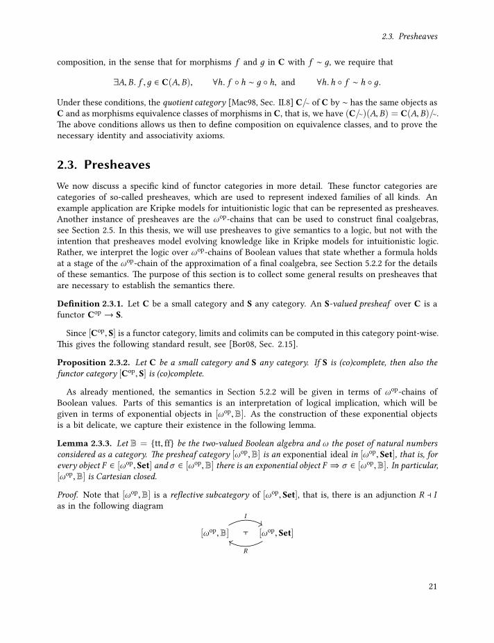
2.3. Presheaves
composition, in the sense that for morphisms f and д in C with f ∼ д, we require that
∃A,B. f ,д ∈ C(A,B), ∀h. f h ∼ д h, and ∀h.h f ∼ h д.Under these conditions, the quotient category [Mac98, Sec. II.8] C/∼ of C by ∼ has the same objects asC and as morphisms equivalence classes of morphisms in C, that is, we have (C/∼)(A,B) = C(A,B)/∼.The above conditions allows us then to define composition on equivalence classes, and to prove thenecessary identity and associativity axioms.
2.3. PresheavesWe now discuss a specific kind of functor categories in more detail. These functor categories arecategories of so-called presheaves, which are used to represent indexed families of all kinds. Anexample application are Kripke models for intuitionistic logic that can be represented as presheaves.Another instance of presheaves are the ωop-chains that can be used to construct final coalgebras,see Section 2.5. In this thesis, we will use presheaves to give semantics to a logic, but not with theintention that presheaves model evolving knowledge like in Kripke models for intuitionistic logic.Rather, we interpret the logic over ωop-chains of Boolean values that state whether a formula holdsat a stage of the ωop-chain of the approximation of a final coalgebra, see Section 5.2.2 for the detailsof these semantics. The purpose of this section is to collect some general results on presheaves thatare necessary to establish the semantics there.
Definition 2.3.1. Let C be a small category and S any category. An S-valued presheaf over C is afunctor Cop → S.
Since [Cop, S] is a functor category, limits and colimits can be computed in this category point-wise.This gives the following standard result, see [Bor08, Sec. 2.15].
Proposition 2.3.2. Let C be a small category and S any category. If S is (co)complete, then also thefunctor category [Cop, S] is (co)complete.
As already mentioned, the semantics in Section 5.2.2 will be given in terms of ωop-chains ofBoolean values. Parts of this semantics is an interpretation of logical implication, which will begiven in terms of exponential objects in [ωop,B]. As the construction of these exponential objectsis a bit delicate, we capture their existence in the following lemma.
Lemma 2.3.3. Let B = tt, ff be the two-valued Boolean algebra and ω the poset of natural numbersconsidered as a category. The presheaf category [ωop,B] is an exponential ideal in [ωop, Set], that is, forevery object F ∈ [ωop, Set] and σ ∈ [ωop,B] there is an exponential object F ⇒ σ ∈ [ωop,B]. In particular,[ωop,B] is Cartesian closed.
Proof. Note that [ωop,B] is a reflective subcategory of [ωop, Set], that is, there is an adjunction R ⊣ Ias in the following diagram
[ωop,B] [ωop, Set]
I
R
⊣
21

Chapter 2. Preliminaries
in which the functor I is fully faithful. The inclusion I is given by
I(σ)(n) =
1, σ(n) = tt∅, σ(n) = ff
and the reflector R byR(F )(n) = tt ⇐⇒ F (n) is inhabited.
Clearly, the induced monad L = I R on [ωop, Set] preserves finite products, from which be obtainby [Joh02, Prop. A4.3.1] that [ωop,B] is an exponential ideal.
The proof of Lemma 2.3.3 appeals to a rather abstract result. Let us for later reference give anexplicit definition of exponential objects in [ωop,B]. Usually, see [Awo10, Sec. 8.7], exponentialobjects in [Cop, Set] are defined to be
(GF )(U ) = [Cop, Set] (y(U ) × F ,G),
that is, (GF )(U ) is given as the set of natural transformations y(U ) × F ⇒ G. The reason why[ωop,B] has exponential objects is that we can define a map yB : ω → [ωop,B] by
yB(n)(m) B ω(m,n) is inhabited =m ≤ n.
That yB is indeed a functor follows by transitivity of ≤. Since the product in [ωop,B] is given bypoint-wise conjunction, we also denote it by
(σ ∧ τ )(n) B σ(n) ∧ τ (n).
The exponential object for σ ,τ ∈ [ωop,B] is then given by
(σ ⇒ τ )(n) = [ωop,B] (yB(n) ∧ σ ,τ ) is inhabited= ∀m ∈ N. (yB(n)(m) ∧ σ(m)) =⇒ τ (m)
= ∀m ∈ N. (m ≤ n ∧ σ(m)) =⇒ τ (m).
A reader who has seen Kripke semantics for intuitionistic logic will certainly recognise that thisdefinition resembles the interpretation of implication in a Kripke frame.
Another ingredient of the semantics in Section 5.2.2 is the so-called later modality that has beentreated category theoretically by Birkedal et al. [Bir+11]. We define it and give some of its properties.
Lemma 2.3.4. Let C be a category with a final object 1, then the map ▷ : [ωop,C] → [ωop,C] given onobjects by
(▷σ)(n) =
1, n = 0
σ(k), n = k + 1
(▷σ)(n ≤ m) =
! : (▷σ)(m)→ 1, n = 0
σ(k ≤ k ′), n = k + 1,m = k ′ + 1
is a functor. Moreover, there is a natural transformation next : Id⇒ ▷.
22

2.3. Presheaves
Proof. First, we check that ▷σ ∈ [ωop,C], if σ ∈ [ωop,C]. Since (▷σ)(0) = 1 is final in C, there is aunique morphism ! : (▷σ)(m)→ (▷σ)(0). For k ∈ N, we have on the other hand that if k + 1 ≤ m,then m = k ′ + 1 with k ′ =m − 1 ∈ N. Thus it is sufficient to define
(▷σ)(k + 1 ≤ k ′ + 1): (▷σ)(k ′ + 1)→ (▷σ)(k + 1).
Since (▷σ)(k + 1) = σ(k) and (▷σ)(k ′ + 1) = σ(k ′), we can thus put (▷σ)(k + 1 ≤ k ′ + 1) =σ(k ≤ k ′). Second, we define ▷ on morphisms. So let σ ,τ ∈ [ωop,C] and let f : σ → τ be a naturaltransformation, we define a natural transformation ▷ f : ▷σ → ▷ τ as follows.
(▷ f )n : (▷σ)(n)→ (▷ τ )(n)
(▷ f )n =
! : 1→ 1, n = 0
fk : σ(k)→ τ (k), n = k + 1
Naturality of ▷ and the functor laws follow from finality of 1.Finally, we need to establish the natural transformation next : Id⇒ ▷. We define it to be
nextσ : σ → ▷σ
nextσ ,n =
! : σ(0)→ 1, n = 0
σ(k ≤ k + 1): σ(k + 1)→ σ(k), n = k + 1
That next is natural in σ is again proven by finality of 1.
The last integral result to the semantics is that the later modality gives rise to a fixed pointoperator in the presheaf category [ωop,B], called Löb induction by Birkedal et al. [Bir+11].
Lemma 2.3.5. Let σ ∈ [ωop,B]. There is a morphism (▷σ ⇒ σ)→ σ in [ωop,B].
Proof. A very quick proof goes by using the fact that for any U ∈ [ωop, Set] there is a morphism(▷U ⇒ U ) → U in [ωop, Set], see [Bir+11], and then appealing by to the fact that [ωop,B] is areflective subcategory of [ωop, Set]. For convenience, we give a direct proof here though.
Let σ ∈ [ωop,B] and n ∈ N. We need to to show that if (▷σ ⇒ σ)(n) holds, then σ(n) holds. Thisis shown by induction on n. Recall that
(▷σ ⇒ σ)(n) = ∀m ∈ N. (m ≤ n ∧ (▷σ)(m)) =⇒ σ(m).
For n = 0, we have that m ≤ n only if m = 0, and that (▷σ)(0) = tt. Thus, (▷σ ⇒ σ)(n) = σ(0),as required. Suppose now that n = k + 1. The assumption reads then as
(▷σ ⇒ σ)(k + 1) = ∀m ∈ N. (m ≤ k + 1 ∧ (▷σ)(m)) =⇒ σ(m).
In particular, we have that ∀m ∈ N. (m ≤ k∧(▷σ)(m)) =⇒ σ(m), fromwhich be derive by inductionthat σ(k) holds. Using the assumption again with m = k + 1, we obtain σ(k) =⇒ σ(k + 1). Thus,we have σ(k + 1). By this induction, σ(n) holds for all n ∈ N if (▷σ ⇒ σ)(n) holds. Hence, thereis a morphism (▷σ ⇒ σ)→ σ .
23

Chapter 2. Preliminaries
2.4. FibrationsThe next category theoretical notion we need are fibrations. Fibrations are an elegant way ofcapturing the fact that in a (higher-order) predicate logic the variables range over some collection ofdata. These variables are typically assigned some sorts, as the validity of a proposition often dependson the data its variables range over. For instance, let P(x) B “x has a maximal element”. First ofall, we need to know what “element of” in this case means, so let us say, for example, that x rangesover lists, and that “element of” means occurrence in a list. Next, what is the meaning of “maximal”here? A possibility is that x ranges over non-empty, finite lists of natural numbers and we can usethe usual order on the natural numbers. Then for any such list u, the proposition P(u) has a sensibleinterpretation and is in fact true. It would not be universally true if we had, for example, x assumedto range over streams of natural numbers, as these have no maximal element. Finally, P(u) wouldeven be nonsensical if u would be a list over some non-ordered structure (leaving things like thewell-ordering theorem aside). This way of assigning types is exactly what we will use fibrations forin Chapter 6. We will also discuss the intention of using fibrations further there. For now we willjust go through the technical background.
Definition 2.4.1. Let P : E → B be a functor, where the E is called the total category and B thebase category. We say for u : I → J in B that a morphism f : A → B in E is cartesian over u,provided that i) P f = u, and ii) for all д : C → B in E and v : PC → I with Pд = u v there isa unique h : C → A such that f h = д. For P to be a fibration, we require that for every B ∈ Eand u : I → PB in B, there is a cartesian morphism f : A→ B over u. Finally, a fibration is cloven,if it comes with a unique choice for A and f , in which case we denote A by u∗ B and f by u B, asdisplayed in the following diagram.
C
u∗ B B E
PC
I PB B
д
!hu B
PPд
vu
On cloven fibrations, we can define for each u : I → J in B a functor, the reindexing along u, asfollows. Let us denote by PI the category having objects A with P(X ) = I and morphisms f : A→ Bwith P(f ) = idI . We call PI the fibre above I . The assignment of u∗ B to B for a cloven fibrationcan then be extended to a functor u∗ : PJ → PI . Moreover, one can show that id∗I IdPI and(v u)∗ u∗ v∗. In this work, we are often interested in split fibrations, which are cloven fibrationssuch that the above isomorphisms are equalities, that is, id∗I = IdPI and (v u)∗ = u∗ v∗.
Example 2.4.2 (See [Jac99]). Important examples of fibrations arise from categories with pullbacks.Let C be a category and C→ be the arrow category as in Section 2.2. We can then define a functorcod : C→ → C by cod(f : X → Y ) = Y . This functor turns out to be a fibration, the codomainfibration, if C has pullbacks, where the fibre of cod above an object A ∈ C is isomorphic to the slicecategory C/A. If we are given a choice of pullbacks, then cod is also cloven.
The split variant of this construction is given by the category of set-indexed families over C.
24
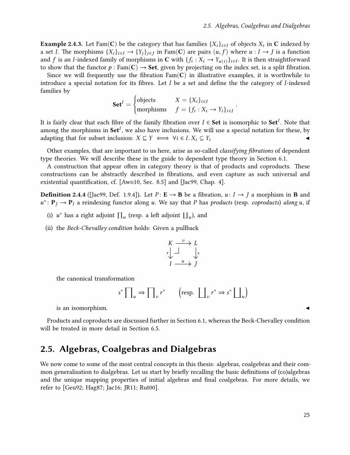
2.5. Algebras, Coalgebras and Dialgebras
Example 2.4.3. Let Fam(C) be the category that has families Xi i ∈I of objects Xi in C indexed bya set I . The morphisms Xi i ∈I → Yj j ∈J in Fam(C) are pairs (u, f ) where u : I → J is a functionand f is an I -indexed family of morphisms in C with fi : Xi → Yu(i)i ∈I . It is then straightforwardto show that the functor p : Fam(C)→ Set, given by projecting on the index set, is a split fibration.
Since we will frequently use the fibration Fam(C) in illustrative examples, it is worthwhile tointroduce a special notation for its fibres. Let I be a set and define the the category of I -indexedfamilies by
SetI =
objects X = Xi i ∈Imorphisms f = fi : Xi → Yi i ∈I
.
It is fairly clear that each fibre of the family fibration over I ∈ Set is isomorphic to SetI . Note thatamong the morphisms in SetI , we also have inclusions. We will use a special notation for these, byadapting that for subset inclusion: X ⊑ Y ⇐⇒ ∀i ∈ I .Xi ⊆ Yi
Other examples, that are important to us here, arise as so-called classifying fibrations of dependenttype theories. We will describe these in the guide to dependent type theory in Section 6.1.
A construction that appear often in category theory is that of products and coproducts. Theseconstructions can be abstractly described in fibrations, and even capture as such universal andexistential quantification, cf. [Awo10, Sec. 8.5] and [Jac99, Chap. 4].
Definition 2.4.4 ([Jac99, Def. 1.9.4]). Let P : E→ B be a fibration, u : I → J a morphism in B andu∗ : PJ → PI a reindexing functor along u. We say that P has products (resp. coproducts) along u, if
(i) u∗ has a right adjoint∏
u (resp. a left adjoint⨿
u ), and
(ii) the Beck-Chevalley condition holds: Given a pullback
K L
I J
v
r s
u
the canonical transformation
s∗∏
u⇒
∏vr ∗
(resp.
⨿vr ∗ ⇒ s∗
⨿u
)is an isomorphism.
Products and coproducts are discussed further in Section 6.1, whereas the Beck-Chevalley conditionwill be treated in more detail in Section 6.5.
2.5. Algebras, Coalgebras and DialgebrasWe now come to some of the most central concepts in this thesis: algebras, coalgebras and their com-mon generalisation to dialgebras. Let us start by briefly recalling the basic definitions of (co)algebrasand the unique mapping properties of initial algebras and final coalgebras. For more details, werefer to [Geu92; Hag87; Jac16; JR11; Rut00].
25

Chapter 2. Preliminaries
Definition 2.5.1. Let C and D be categories and F ,G : C → D functors. An (F ,G)-dialgebrais a morphism c : FA → GA in D, where A is an object in C. Given dialgebras c : FA → GAand d : FB → GB, a morphism h : A→ B is said to be a (dialgebra) homomorphism from c to d , ifGh c = d Fh. We can form a category DiAlg(F ,G) of (F ,G)-dialgebras and their homomorphisms.A dialgebra is said to be initial (resp. final) if it is an initial (resp. final) object in DiAlg(F ,G).
A word about terminology: Given a dialgebra d : FB → GB, we call the unique homomorphismfrom an initial (F ,G)-dialgebra into d the inductive extension of d . Dually, the unique homomorphisminto a final dialgebra is called the coinductive extension of d .
Let us discuss an example of a dialgebra in the category of sets.Example 2.5.2. Let F ,G : Set→ Set × Set be given by F = ⟨1, Id⟩ and G = ⟨Id, Id⟩, that is, F mapsa set X to the pair (1,X ) in the product category. Similarly, G, the diagonal functor, maps X to(X ,X ). Now, let z : 1 → N and s : N → N be the constant zero map and the successor on naturalnumbers, respectively. It is then easy to see that (z, s) : F (N)→ G(N) is an initial dialgebra.
We will often need the case of dialgebras, in which F or G is the identity functor.Definition 2.5.3. Let H : C → C be a functor. An algebra is a morphism a : HX → X in C and acoalgebra is a morphism c : X → HX . The notion of homomorphism of algebras and coalgebras is thesame as for dialgebras with the choices G = Id and F = Id, respectively. We denote by Alg(H) andCoAlg(H) the categories of algebras and coalgebras with their homomorphisms. These categoriesmay have initial (resp. final) objects, to which we refer as initial algebra (resp. final coalgebra).
The following is an important result that shows the relation between initial algebras and leastfixed points, and final coalgebras and greatest fixed points in ordered structures like lattices.Lemma 2.5.4 (Lambek). Let F : C → C be a functor. Every initial algebra α : FA → A and finalcoalgebra ξ : B → FB is an isomorphism. In other words, the objects A and B are fixed points, in the sensethat FA A and FB B.
Now that we know that initial algebras and final coalgebras generalise fixed points, one may askhow these can be constructed. The way that is most important to us here are the so-called initialand final chain constructions.Definition 2.5.5. Let F : C → C be a functor. If C has an initial object 0, then the initial chain isthe functor −→F : ω → C from the ordinal ω considered as a poset to C defined as in the followingdiagram. Here, ! denotes the unique morphism out of 0.
−→F : 0 F (0) F 2(0) F 3(0) · · ·! F (!) F 2(!) F 3(!)
More precisely, this means that −→F is defined on objects by−→F (0) = 0 −→
F (k + 1) = F(−→F (k)
)and on morphisms by −→F (0 ≤ n) = ! : 0→ Fn(0) and −→F (k +1 ≤ n) = F
(−→F (k ≤ n)
). Dually, if C has
a final object 1, then there is a functor ←−F : ωop → C, the final chain, as in the following diagram.←−F : 1 F (0) F 2(0) F 3(0) · · ·! F (!) F 2(!) F 3(!)
We say that the initial and final chain stabilise, if F(colim−→F
) colim−→F and F
(lim←−F
) lim←−F .
26
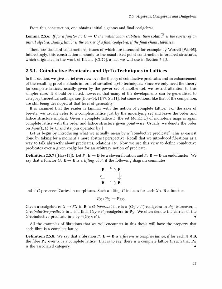
2.5. Algebras, Coalgebras and Dialgebras
From this construction, one obtains initial algebras and final coalgebras.
Lemma 2.5.6. If for a functor F : C → C the initial chain stabilises, then colim−→F is the carrier of aninitial algebra. Dually, lim←−F is the carrier of a final coalgebra, if the final chain stabilises.
These are standard constructions, issues of which are discussed for example by Worrell [Wor05].Interestingly, this construction amounts to the usual fixed point construction in ordered structures,which originates in the work of Kleene [CC79], a fact we will use in Section 5.2.2.
2.5.1. Coinductive Predicates and Up-To Techniques in LatticesIn this section, we give a brief overview over the theory of coinductive predicates and an enhancementof the resulting proof methods in form of so-called up-to techniques. Since we only need the theoryfor complete lattices, usually given by the power set of another set, we restrict attention to thissimpler case. It should be noted, however, that many of the developments can be generalised tocategory theoretical settings, see [Bon+14; HJ97; Sta11], but some notions, like that of the companion,are still being developed at that level of generality.
It is assumed that the reader is familiar with the notion of complete lattice. For the sake ofbrevity, we usually refer to a complete lattice just by the underlying set and leave the order andlattice structure implicit. Given a complete lattice L, the set Mon(L,L) of monotone maps is againcomplete lattice with the order and lattice structure given point-wise. Usually, we denote the orderon Mon(L,L) by ⊑ and its join operator by
⊔.
Let us begin by introducing what we actually mean by a “coinductive predicate”. This is easiestdone by taking for a moment a more abstract perspective. Recall that we introduced fibrations as away to talk abstractly about predicates, relations etc. Now we use this view to define coinductivepredicates over a given coalgebra for an arbitrary notion of predicate.
Definition 2.5.7 ([Has+13]). Let P : E→ B be a cloven fibration and F : B→ B an endofunctor. Wesay that a functor G : E→ E is a lifting of F , if the following diagram commutes
E E
B BP
G
P
F
and if G preserves Cartesian morphisms. Such a lifting G induces for each X ∈ B a functor
GX : PX → PFX .
Given a coalgebra c : X → FX in B, a G-invariant in c is a (GX c∗)-coalgebra in PX . Moreover, aG-coinductive predicate in c is a final (GX c∗)-coalgebra in PX . We often denote the carrier of theG-coinductive predicate in c by ν(GX c∗).
All the examples of fibrations that we will encounter in this thesis will have the property thateach fibre is a complete lattice.
Definition 2.5.8. We say that a fibration P : E→ B is a fibre-wise complete lattice, if for each X ∈ B,the fibre PX over X is a complete lattice. That is to say, there is a complete lattice L, such that PXis the associated category.
27
Chapter 2. Preliminaries
The importance of this definition comes from the fact that we can find by the Knaster-Tarskitheorem for any lifting to a fibre-wise complete lattice the corresponding coinductive predicate.
Proposition 2.5.9. Let P : E → B be a fibration that is a fibre-wise complete lattice. For any functorF : B→ B, any lifting G of F and any coalgebra c : X → FX , the G-coinductive predicate in c exists.
We now restrict attention to a single complete lattice L and a monotone map Φ: L → L, whichshould be thought of as being of the form GX c∗. The idea of Φ is that it allows us to describeinvariants. In particular, we obtain the following standard proof method for coinductive predicates:If p ≤ Φ(p), that is, p is a Φ-invariant, then p ≤ νΦ. This is a useful proof method that has foundmany applications. For instance, bisimilarity of transition systems can be described as coinductivepredicate, and the above proof method is then the standard bisimulation proof method [San11].
Often, we find ourselves that an invariant has to be chosen quite large, mostly with elements thatcould be “automatically” added. To overcome this, up-to techniques were introduced in [Mil89] andfurther developed in [Bon+14; Pou07; PS11; Rot15; San98]. A particular class of up-to techniques,the so-called compatible ones, has emerged in this development. The significance of this class comesfrom the fact that it is closed under composition and other lattice operations.
Definition 2.5.10. A Φ-compatible up-to technique is a monotone map T : Ln → Lm with T Φ×n ⊑Φ×m T , where Φ×n : Ln → Ln is given by point-wise application of Φ to the elements in the productlattice Ln . We say that p ∈ L is a Φ-invariant up to T , if p×m ⊑ Φ(T (p×n)).
The following result makes precise the importance of compatible up-to techniques that we men-tioned above: They are sound enhancement of the coinductive proof method and they can becomposed. This result can be found, for example, in [Bon+14; Pou07; Rot+17].
Lemma 2.5.11.
1. If T : L→ L is Φ-compatible and p ∈ L is an invariant up to T , then p ≤ νΦ (Soundness).
2. If T1 : Ln → Lm and T2 : Lm → Lk are Φ-compatible, then so is their composition T2 T1.
3. If T1 : Ln → Lm and T2 : Ln → Lm are Φ-compatible, then so is T1 ⊔T2.
4. Both the identity id : L→ L and Φ itself are Φ-compatible.
Proof. For the first item, one defines a monotone map Tω : L→ L of all finite iterations of T , whichis given by Tω =
⊔n∈NT
n . It can then be shown that if p is an invariant up to T , then Tω(R) isa Φ-invariant. For details see [Bon+14; Rot15]. The second and third item are given by an easycalculation using compatibility and monotonicity:
(T2 T1) Φ ⊑ T2 Φ T1 ⊑ Φ (T2 T1).
and for p ∈ Ln
((T1 ⊔T2) Φ)(p) = T1(Φ(p)) ∨T2(Φ(p)) ≤ Φ(T1(p)) ∨ Φ(T2(p))≤ Φ(T1(p) ∨T2(p)) = (Φ (T1 ⊔T2))(p).
Finally, the compatibility of id is given by id Φ = Φ = Φ id, and the compatibility of Φ isimmediate by the definition of compatibility.
28

2.6. 2-Categories
The advantage of compatible up-to techniques over other techniques that are merely sound, thefirst property in Lemma 2.5.11, is that they can be composed. This allows us to break up proofs ofsoundness into simpler techniques and then combine these techniques in the proof of an invariant.A problem is though that we need to carefully set up the combination of up-to techniques beforestarting the proof. We can resolve this issue by using a universal, compatible up-to technique, theso-called companion [Pou16; PR17].
Definition 2.5.12. The companion of Φ is defined by
γΦ B⊔
T ∈Mon(L,L)T Φ⊑ΦT
T .
The point of the companion is that it is the largest compatible up-to technique for Φ. Thus, wecan use in a proof of invariance the companion instead of having to establish explicitly all the up-totechniques that we use in that proof. This is captured by the following lemma.
Lemma 2.5.13. The companion of Φ is the largest compatible up-to technique and idempotent:
• γΦ is Φ-compatible
• If T is Φ-compatible, then T ⊑ γΦ.
• γΦ γΦ ⊑ γΦ
Proof. That γΦ is the largest compatible functions, the first and second property, is given immediatelyby definition, since the join ranges over all compatible maps. The third property follows from thefact that compatible functions are closed under composition and the other two properties.
2.6. 2-CategoriesA useful tool for describing the difference between the computational behaviour and observablebehaviour of programs are 2-categories. The goal of this section is to carefully set up the terminologyof 2-category theory, which can be a bit confusing at times. We begin with the basic definition ofa (strict) 2-category, which can be found for example in [Bor08] or [Lei04].
Definition 2.6.1. A (strict) 2-category C is a category enriched over the category Cat of all categories.This means that for all objects A and B of C there is a category of morphism C(A,B), and for allobjects A,B,C there are composition and unit functors
cABC : C(A,B) × C(B,C)→ C(A,C) and uA : 1→ C(A,A),
subject to the associativity and unit axioms in the following two diagrams.
C(A,B) × C(B,C) × C(C,D) C(A,B) × C(B,D)
C(A,C) × C(C,D) C(A,D)
Id×cBCD
cABC×Id cABD
cACD
29

Chapter 2. Preliminaries
1 × C(A,B) C(A,B) C(A,B) × 1
C(A,A) × C(A,B) C(A,B) C(A,B) × C(B,B)
uA×Id
Id×uAcAAB cABB
The reason why the 2-categories we defined in Definition 2.6.1 carry the prefix “strict” is thatthere exist various definitions of a category with 2-morphisms. Rather one is faced with a choicein which form the composition of 1-morphisms is unital and associative. For a strict 2-category werequired that these take the form of equalities. However, one can also require instead that therefor all f ,д,h there merely are invertible 2-morphisms α : h (д f )⇒ (h д) f , γ1 : id f ⇒ fand γ2 : f id ⇒ f , which satisfy some coherence conditions. Such a structure is then called abicategory or weak 2-category. For example, given a category C with pullbacks, there is a bicategorySpan(C) that has as objects the objects of C, spans A ←− B −→ C as morphisms and morphisms ofspans as 2-morphisms. Associativity cannot hold strictly in Span(C) because pullbacks are onlyunique up-to isomorphism.
A strict 2-category C can equivalently be described algebraically as follows [Bor08]. First of all,C consists of the following data:
• a collection of objects (0-cells), denoted by A,B, . . . ;
• 1-morphisms (1-cells) between objects, denoted by f : A→ B; and
• 2-morphisms (2-cells) between 1-morphisms, denoted by α : f ⇒ д.
Just like we can compose morphisms in ordinary categories, 1- and 2-morphisms can be composedin 2-categories. Clearly, we have different ways of composing these though. So let us go throughthe different kinds of compositions and their interactions.
Given 1-morphisms f : A→ B and д : B → C there is a morphism д f : A→ C given by cABC (f ,д),just as for ordinary categories. For 2-morphisms though there are two ways of composing them, asindicated in the following diagrams.
A B
f
д
h
α
βA B C
f1
д1
f2
д2
γ δ
In the left diagram we are able to compose α and β along the indicated 1-morphisms to β 1 α : f ⇒ h,where the subscript 1 indicates that we compose along 1-morphisms. This is the so-called verticalcomposition of α and β , and is given by composition in C(A,B). In the diagram on right we composealong objects. This horizontal composition of γ and δ results from the action of cABC morphisms. Itis usually denoted by δ 0 γ : f2 f1 ⇒ д2 д1, where the 0 subscript indicates that we composealong objects (0-cells). We often write γδ instead of δ 0 γ , which relates the horizontal compositionbetter to the geometry of diagrams.
Finally, all the above compositions are associative, the compositions and 1 are unital, and thetwo compositions of 2-morphisms interact through the exchange law as follows.
30

2.6. 2-Categories
• For every object A there is an identity morphisms idA = uA(∗) that is neutral with respect tocomposition, that is, idB д = д = д idA for all morphisms д : A→ B;
• For all 1-morphisms f , there are 2-morphisms idf that are neutral for 1;
• All the compositions of 1- and 2-morphisms are associative;
• The exchange law for the composition of 2-morphisms holds, that is, we have
(β2 1 α2) 0 (β1 1 α1) = (β2 0 β1) 1 (α2 0 α1),
for 2-morphisms as in the following diagram.
A B C
α1
β1
α2
β2
Since no other forms of 2-categories, like weak 2-categories or bicategories, do not appear in thisthesis, we follow Lack [Lac10] and refer to strict 2-categories just as 2-categories,
Example 2.6.2. We just list a few examples of 2-categories. Further examples, a discussion of2-categories and more references can be found in [Lac10].
• We can extend the (large) category Cat of categories and functors with natural transformationsas 2-cells, which we denote by abuse of notation also as Cat. This is the prototypical exampleof a 2-category.
• There is a sub-2-category of Cat, which has the same objects and morphisms, but the 2-morphisms are only the natural isomorphisms.
• A similar example is the 2-category Adj that has again categories as objects, but now ad-junctions as 1-morphisms and morphism between adjunctions, called conjugate pairs, as2-morphisms.
• There are of course also examples of 2-categories that do not not just have categories asobjects. One of these is an extension of the category of topological spaces.Let I be the unit interval of the real numbers. A homotopy between two continuous mapsf ,д : X → Y is a continuous map h : I × X → Y , such that h(0,−) = f and h(1,−) = д.Such homotopies can be composed vertically and horizontally, and there is a homotopy thattakes the role of the identity. The only caveat is that associativity and the unit law forcomposition only hold up-to a homotopy I × (I × X ) → Y . So we end up with a 2-categorythat has topological spaces as objects, continuous maps between spaces as 1-morphisms, andhomotopy-equivalence classes of homotopies between continuous maps as 2-morphisms. Fora few more details see [Bor08, Ex. 7.1.4].
31

Chapter 2. Preliminaries
• Another example is the category PreOrd that has pre-ordered sets (X , ≤X ) as objects andmonotone functions as morphisms. A 2-cell f ⇒ д between two maps f ,д : X → Y exists inPreOrd if f is point-wise smaller than д. Since morphisms are functions, their compositionand identity morphisms are immediate. For 2-cells, note that the vertical composition istransitivity of the point-wise order, and the existence of identities for vertical compositionencodes that the point-wise order is reflexive. To define the horizontal composition, supposewe have
X Y Z
f
f ′
≤
д
д′
≤
Then we can easily calculate from monotonicity of д that for all x ∈ X we have
д(f (x)) ≤Z д(f ′(x)) ≤Z д′(f ′(x)),
thus we can compose the inequalities horizontally to obtain д f ≤ д′ f ′.
In Section 4.2.2 we will see more concrete examples of 2-categories. There, 2-morphisms will allowus to speak about a program equivalence in categorical terms while still retaining information aboutcomputations.
Since the collection of morphisms in a 2-category forms a category, we can talk about isomorphic1-morphisms.
Definition 2.6.3. Let f ,д : A → B be 1-morphisms in a 2-category C. We say that f and д areisomorphic, written f д, if they are isomorphic as objects in Hom (A,B), that is, if there are2-morphisms α : f ⇒ д and β : д⇒ f with α 1 β = id and β 1 α = id.
Definition 2.6.1 might suggest that 2-categories could be studied just as an instance of enrichedcategory theory. The problem with this view is that it locks us into notions of functors and (co)limitsin 2-categories that are usually too strict. For instance, the notion of functor that arises fromenriched category theory requires that the composition of 1-morphisms is strictly preserved, that is,F (д f ) = F (д) F (f ). As it will turn out, we instead need the weaker notion of pseudo-functors,where we only have F (д f ) F (д) F (f ).
Definition 2.6.4. LetC andD be 2-categories. A pseudo-functor F : C→ Dmaps the 0-, 1- and 2-cellsin C to those in D, such that 1-identities and the 1-composition are preserved up-to isomorphism,and 2-identities and 2-compositions are strictly preserved. More precisely, let uC and uD be theunit functors of C and D, respectively, and cC and cD the corresponding composition functors. Thepseudo-functor F consists of
• an object F (A) in D for each object A in C,
• a functor FA,B : C(A,B)→ C(FA, FB) for all objects A and B,
• a natural isomorphism FidA : uDFA ⇒ FA,A uCA for all A,
• a natural isomorphism FABC : cDFA,FB,FC (FA,B × FB,C )⇒ FA,C cCABC for all A, B and C .
32

2.6. 2-Categories
To improve readability, we write FidA instead of (FidA)∗ for ∗ ∈ 1 and F (д, f ) instead of (FABC )(f ,д).Finally, the following three coherence diagrams must commute for all suitable f , д and h.
F (f ) idF (A) F (f )
F (f ) F (idA) F (f idA)
idF (f )FidAF (f , idA)
idF (B) F (f ) F (f )
F (idB) F (f ) F (idB f )
FidB idF (f )F (idB,f )
F (h) F (д) F (f ) F (h д) F (f )
F (h) F (д f ) F (h д f )
idF (h)F (д,f )
F (h,д)idF (f )
F (hд,f )F (h,дf )
We say that F is a strict 2-functor , if all the isomorphisms FidA and F (д, f ) are identities.9
Just as for any ordinary category D there is a hom-functor D : Dop ×D→ Set, we note that thereis the corresponding analogue for 2-categories, see [Bor08, Ex. 7.2.4].
Example 2.6.5. For every 2-category C there is a strict 2-functor Cop ×C→ Cat, where C(A,B) isthe hom-category as in Definition 2.6.1, and for f : A′→ A and д : B → B′ the functor part is
C(f ,д) : C(A,B)→ C(A′,B′)C(f ,д) = cA′BB′(−,д) cA′AB(f ,−),
that is, given by pre-composing with f and post-composing with д as for the ordinary hom-functor.
Proof. Since the composition c is a functor, C(f ,д) is a functor. So it remains to prove the preservationof units and composition. It follows easily from the unit laws in Definition 2.6.1 that C(id, id) = id.From the associativity law it also follows that cA′BB′(−,д) cA′AB(f ,−) = cA′AB′(f ,−) cABB′(−,д),which in turn gives us for all f ′,д′ that C(f ′ f ,д д′) = C(f ,д) C(f ′,д′).
2.6.1. Adjunctions, Products, Coproducts and Exponents in 2-CategoriesHaving introduced 2-categories and a notion of morphism between them (pseudo-functors), it is onlynatural to study tighter connections between 2-categories, namely that of pseudo-adjunctions. Thesepseudo-adjunctions will also allow us to introduce suitable generalisations of limits and colimits to2-categories.
Unfortunately, the machinery to describe suitably weak adjunctions between 2-categories andlimits and colimits gets very technical because of the necessary coherence conditions that have tobe satisfied. On the positive side though, we have that many of the technicalities are still simpler incomparison to what we would find in, for example, bicategories. We will always give some intuitionabout how the weakened notions compare to those for ordinary categories. This should give at leastan idea to the reader what we are up to, so that the technicalities can be skipped for the most part.
Definition 2.6.6. Let F ,G : C→ D be pseudo-functors. A pseudo-natural transformation α : F ⇒ Gis given by the following data:
33

Chapter 2. Preliminaries
• a morphism αA : FA→ GA for every object A ∈ C, and
• for all objects A,B ∈ C a natural isomorphism
αA,B : C(αA, idGB) GA,B ⇒ C(idFA,αB) FA,B ,
where C is the 2-functor obtained in Example 2.6.5.
Moreover, the following two coherence diagrams must commute.
αA idGA αA G(idA) αA
αA idFA αA F (idA)
GidA idαA
αidAidαA FidA
Gд Gf αA Gд αA F f αA Fд F f
G(д f ) αA αA F (д f )
idGдαf
G(д,f )idαA
αд idGf
idαA F (д,f )αдf
As before, we obtain a strict version by requiring that αA,B is the identity.
Definition 2.6.7. A pseudo-adjunction between 2-categories C and D is a pair of pseudo-functorsF : C→ D and G : D→ C, such that for each A ∈ C and B ∈ D there is a equivalence of categories
D(FA,B) ≃ C(A,GB)
that is pseudo-natural in both A and B. We say that F is left pseudo-adjoint to G, and denote thisby F ⊣ G.
Definition 2.6.8. We say that a 2-category C has binary pseudo-coproducts and pseudo-products, ifthere is a left pseudo-adjoint + ⊣ ∆, respectively a right pseudo-adjoint ∆ ⊣ ×, to the diagonal2-functor ∆: C → C × C. Moreover, a 2-category with pseudo-products C is said to have pseudo-exponents if for each object A ∈ C, the one-sided product pseudo-functor (−) × A : C → C has aright pseudo-adjoint (−) ×A ⊢ (−)A. Finally, an object ⊤ in C is said to be pseudo-final, if for everyobject A in C we have C(A,⊤) ≃ 1, that is, the hom-category C(A,⊤) is equivalent to the finalcategory.
Definition 2.6.8 is very compact and generalises directly adjunctions for ordinary categories, butis also very dense at that. So let us unfold what the definition for pseudo-products actually says.Let A and B be objects in C. Then there is an object A × B with projections π1 : A × B → A andπ2 : A × B → B, such that
• for all f : C → A and д : C → B there is an h : C → A × B with isomorphism π1 h f andπ2 h д, and
• for all h,k : C → A × B and 2-morphisms α : π1 h ⇒ π1 k and β : π2 h ⇒ π2 k , there isa unique γ : h ⇒ k such that π1γ = α and π2γ = β .
34

2.6. 2-Categories
For pseudo-coproducts we have of course the dual situation. So let us instead spell out thedefinition of pseudo-exponents. Let A be an object in C. We denote the functors that mediate thehom-categories for the exponential objects by
αB,C : C(B ×A,C) ≃ C(B,CA) : βB,C .
The pseudo-naturality of α reads then for u : B′→ B, v : C → C ′ and k : B ×A→ C as
αB′,C ′(v k u ×A) = αB′,C ′(C(u ×A,v)(k)) C(u,vA)(αB,C (k))= vA α(k) u
(2.1)
We now have for each object B an evaluation morphism evB : BA × A→ B that is given by evB =βBA,B(idBA). Moreover, for every f : B × A → C we find a morphism λ f : A → CB by puttingλ f = αB,C (f ). This morphism has then the expected property, only weakening the usual one forexponents:
evC (λ f ×A) f .
To see this, we can just give the usual argument, only replacing identities with isomorphisms. First,we have for д B αB,C (evC (λ f ×A))
д = αB,C (evC (λ f ×A))= αB,C (β(id) (α(f ) ×A)) by definition αB,C (β(id)) α(f ) (2.1) with v = id,u = α(f ),k = β(id) α(f ) α , β form an equivalence.
This gives us nowevC (λ f ×A) β(α(evC (λ f ×A))) β(д) f ,
as required. Using similar reasoning, we can now also show that the abstraction is unique up tounique isomorphism, just as we have seen that the pairing for pseudo-products is unique up tounique isomorphism.
2.6.2. Algebras and Coalgebras for Pseudo-FunctorsDefinition 2.6.9. Given a 2-category C and a pseudo-functor F : C → C, we call a morphismc : X → FX an F -coalgebra. A pseudo-homomorphism of F -coalgebras c : X → FX and d : Y → FYis a morphism h : X → Y , such that there is an 2-isomorphism φh : d h ⇒ Fh c . F -algebras andtheir homomorphisms are given by duality, with the 2-isomorphism being denoted by θ .
Lemma 2.6.10. Let C be a 2-category and F : C→ C be a pseudo-functor. There are 2-categories Alg(F )and CoAlg(F ) of algebras and, respectively, coalgebras and their pseudo-homomorphisms.
Proof. We carry out the proof for CoAlg(F ), that for Alg(F ) follows by duality. The 2-categoryCoAlg(F ) is given by
CoAlg(F ) =
objects: pairs (X , c : X → FX ) of objects and coalgebras in Cmorphisms: pseudo-homomorphisms (X , c)→ (Y ,d)
2-cells: all 2-morphisms of C between pseudo-homomorphisms
35
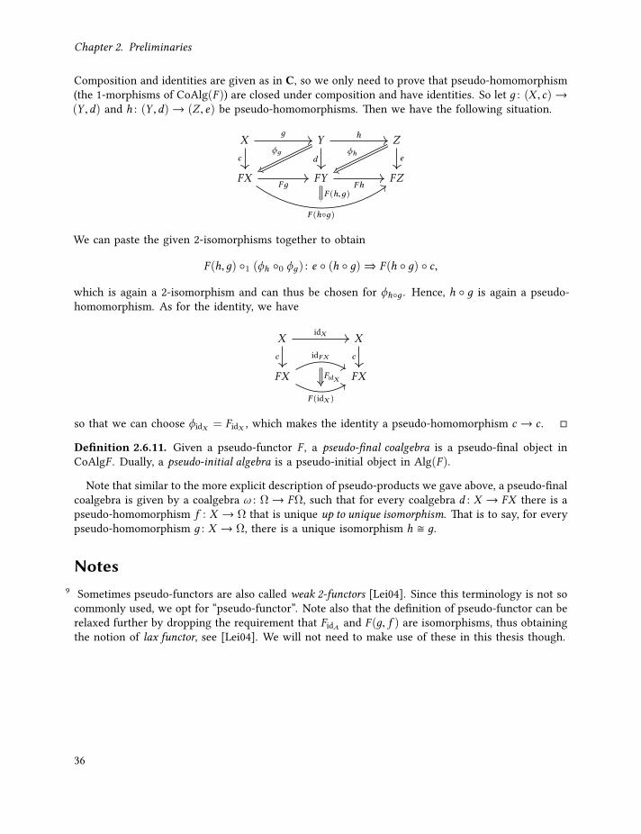
Chapter 2. Preliminaries
Composition and identities are given as in C, so we only need to prove that pseudo-homomorphism(the 1-morphisms of CoAlg(F )) are closed under composition and have identities. So let д : (X , c)→(Y ,d) and h : (Y ,d)→ (Z , e) be pseudo-homomorphisms. Then we have the following situation.
X Y Z
FX FY FZ
c
д
d
h
φдe
φh
Fд
F (hд)
FhF (h,д)
We can paste the given 2-isomorphisms together to obtain
F (h,д) 1 (φh 0 φд) : e (h д)⇒ F (h д) c,
which is again a 2-isomorphism and can thus be chosen for φhд . Hence, h д is again a pseudo-homomorphism. As for the identity, we have
X X
FX FX
c
idX
cidFX
F (idX )
FidX
so that we can choose φidX = FidX , which makes the identity a pseudo-homomorphism c → c .
Definition 2.6.11. Given a pseudo-functor F , a pseudo-final coalgebra is a pseudo-final object inCoAlgF . Dually, a pseudo-initial algebra is a pseudo-initial object in Alg(F ).
Note that similar to the more explicit description of pseudo-products we gave above, a pseudo-finalcoalgebra is given by a coalgebra ω : Ω→ FΩ, such that for every coalgebra d : X → FX there is apseudo-homomorphism f : X → Ω that is unique up to unique isomorphism. That is to say, for everypseudo-homomorphism д : X → Ω, there is a unique isomorphism h д.
Notes9 Sometimes pseudo-functors are also called weak 2-functors [Lei04]. Since this terminology is not socommonly used, we opt for “pseudo-functor”. Note also that the definition of pseudo-functor can berelaxed further by dropping the requirement that FidA and F (д, f ) are isomorphisms, thus obtainingthe notion of lax functor, see [Lei04]. We will not need to make use of these in this thesis though.
36

CHAPTER 3
Inductive-Coinductive Programming
We can forgive a man for making a useful thing as long as he does not admire it. The only excuse for makinga useless thing is that one admires it intensely.
— Oscar Wilde, “The Picture of Dorian Gray”, 1891.
Though this thesis is about mixed inductive-coinductive reasoning, we first need something toreason about. Given that the focus of this thesis lies on proofs that can be checked by computers,a good starting point is the reasoning about programs. So the goal of this chapter is to establishprogramming calculi that allow us manipulate inductive-coinductive data.
In Section 3.1, we introduce a typed λ-calculus λµν that has at its heart iteration and coiterationschemes for defining functions out of inductive types and into coinductive types, respectively. Thiscalculus comes with a notion of computation that is defined through a reduction relation, whichallows us to execute programs on data. The reduction relation enjoys very good properties likeconfluence, progression and strong normalisation. However, the calculus itself is difficult to use,especially once we start mixing inductive and coinductive types.
This leads us to consider in Section 3.2 another calculus λµν= in which the iteration and coiterationschemes are replaced by recursive equations. For example, we can define in λµν= the addition ofnatural numbers simply by case distinction and recursion: 0+m =m and (sucn)+m = suc(n+m),whereas in λµν we have to use higher-order iteration. This makes it much easier to specify programsin the calculus, but we lose the property that all computations are terminating, that is, there areprograms on which the reduction relation associated with the calculus is not strongly normalisinganymore. We come back to this problem in Chapter 4.
In the last Section 3.3, we relate the two calculi by translating the terms of λµν to terms in λµν=.This shows that the iteration and coiteration schemes can be emulated as recursive equations inλµν=. Moreover, this also allows us to infer properties, like confluence, of λµν from those of λµν=.
Original Publication The calculus presented in Section 3.1 has not appeared in any of the author’spublications but similar calculi can be found throughout the literature. We will discuss this inSection 3.4 at the end of the chapter. The content of Section 3.2 is largely based on Basold andHansen [BH16], which considers a variation of the copattern calculus given by Abel et al. [Abe+13].
3.1. Programming with Iteration and CoiterationIn this section we give a first introduction to mixed inductive-coinductive programming by devisinga simply typed calculus that features both inductive and coinductive data types. The calculus is setup so as to avoid issues related to program termination, something we will deal with in Section 3.2and Section 4.1. For easier reference, we will refer to the calculus presented in this section as λµνand that presented in Section 3.2 as λµν=.
37

Chapter 3. Inductive-Coinductive Programming
X ∈ ΘΘ ⊩ X : Ty Θ ⊩ 1 : Ty
Θ ⊩ A : Ty Θ ⊩ B : TyΘ ⊩ A+ B : Ty
Θ ⊩ A : Ty Θ ⊩ B : TyΘ ⊩ A × B : Ty
⊩ A : Ty Θ ⊩ B : TyΘ ⊩ A→ B : Ty
Θ,X ⊩ A : TyΘ ⊩ µX .A : Ty
Θ,X ⊩ A : TyΘ ⊩ νX .A : Ty
Figure 3.1.: Type construction rules
3.1.1. Types and Terms of the Calculus λµνWe first introduce the types with respect to which the calculus will be typed.
Definition 3.1.1. Let TyVar be a countably infinite set of type variables, elements of which wedenote by X ,Y ,Z possibly with subscript indices. We say that A is a raw type if it is generated bythe following grammar.
A,B F X | 1 | A+ B | A × B | A→ B | µX .A | νX . B
To avoid ambiguities, we adopt the following common conventions for binding of type operators.First of all, one may always use parentheses to disambiguate. Further, × binds stronger than →,which binds stronger than +; × and + are left-associative; → is right-associative; and the bindingof fixed point types extends from the dot all the way to the right.
If a raw type A is strictly positive, that is, if type variables never occur left of an arrow, then Ais a type. More precisely, A is a type if for some sequence Θ of type variables, Θ ⊩ A : Ty can bederived inductively from the rules in Figure 3.1. In case Θ is empty, we say that A is closed type.The set of all closed types is denoted by Ty. Sometimes we have to be a bit more precise about thevariables that are actually used in a type. To this end, we define for a (raw) type A the set fv(A)of free variables, by fv(X ) = X , fv(1) = ∅ and in the other cases in the obvious way. Finally, wecall a map υ : Θ→ Ty a type substitution and denote the set of all such substitutions by TySubst(Θ).The empty type substitution is denoted by ().
Let us give a few examples of Definition 3.1.1.
Example 3.1.2. The first example is a type that is supposed to resemble the empty set:
0 B µX .X .
We will see that the idea of this type is that any potential inhabitant would have to representa non-terminating computation. Since we will exclude such computations, the type will have noinhabitants, as required.
Dually to the empty type, we can define a type that corresponds to a singleton set by
1′ B νX .X .
In Example 3.1.6 we show that this type has an inhabitant, but it is only in Chapter 4 that we areable to prove that this inhabitant is canonical, thus that 1′ is isomorphic to 1.
38

3.1. Programming with Iteration and Coiteration
A non-trivial example is the type of natural numbers, which is given by
Nat B µX . 1+ X .
As usual, the idea is that this type has two constructors, one for the number 0 and one for thesuccessor of a given number. We will see this in Example 3.1.7. Streams, on the other hand, arecharacterised by the two destructors of taking the head (first element) of a stream and the tail (theremaining stream after the head). So for a given type A, the type of streams over A is given by thefollowing coinductive type.
Aω B νX .A × XWe expose the head and tail destructors in Example 3.1.8.
These are well-known, classical examples of inductive and coinductive types. Let us now come totypes that properly mix inductive and coinductive types.
Example 3.1.3. One example are streams over given typesA and B in which infinitely many elementsof type A occur, called left-fair streams. These streams can be defined as type by
LFairA B B νX . µY .A × X + B × Y .
Note that this type should be read as νX . (µY . ((A × X ) + (B × Y ))) according to the conventionsin Definition 3.1.1. Another example that illustrates nested fixed points are A-labelled, finitely-branching, potentially infinite, nonempty trees, which are given by
TrA B νX .A × (µY . 1+ X × Y ).
We will come back to these types in Section 3.2.
Finally, non-examples of types are µX .X → X and µX . (X → 1) → 1. Both types are forbiddenbecause the type variable X occurs left of an arrow. The latter type is commonly referred to as a(non-strictly) positive type because X occurs left of an even number of arrows. Positive types canbe acceptable from a computational perspective [Abe04; Gre92; Mat99; Men91; UV96]. However,allowing non-strictly positive types would make a lot of the development in this thesis much harder,especially that in Section 4.1. Thus, we rule out non-strictly positive types here. Note that thefirst type would allow us to embed the untyped λ-calculus into the calculus we introduce below,see [BDS13, Sec. 9.3], and thus would lead to the existence of non-normalising terms.
We now introduce the terms of the calculus λµν .
Definition 3.1.4. Let TeVar be a countably infinite set of term variables, the elements of which wedenote by x ,y, z,x1,x2, . . . The raw terms of λµν are generated by the following grammar.
s, t ,u F ⟨ ⟩ | κ1 t | κ2 t | α t | π1 t | π2 t | ξ t | t s | ⟨t , s⟩| x | λx . t | κ1 x 7→ s ; κ2 y 7→ t u x ,y ∈ TeVar| iterµX .A (x . t) s | coiterνX .A (x . t) s X ⊩ A : Ty
We adopt the usual convention that application is left-associative to again allow for disambiguationof raw terms. This applies also to κ1,π1 etc.
39

Chapter 3. Inductive-Coinductive Programming
(x : A) ∈ Γ(Proj)
Γ ⊢ x : A(1-I)
Γ ⊢ ⟨ ⟩ : 1
i ∈ 1, 2 Γ ⊢ t : A1 ×A2 (×-E)Γ ⊢ πi t : Ai
Γ ⊢ t1 : A Γ ⊢ t2 : B (×-I)Γ ⊢ ⟨t1, t2⟩ : A × B
Γ ⊢ t1 : A→ B Γ ⊢ t2 : A (→-E)Γ ⊢ t1 t2 : B
Γ,x : A ⊢ t : B (→-I)Γ ⊢ λx .t : A→ B
i ∈ 1, 2 Γ ⊢ t : Ai (+-I)Γ ⊢ κi t : A1 +A2
Γ,x : A ⊢ s : C Γ,y : B ⊢ t : C Γ ⊢ u : A+ B(+-E)
Γ ⊢ κ1 x 7→ s ; κ2 y 7→ t u : C
Γ ⊢ t : A[µX .A/X ](µ-I)
Γ ⊢ α t : µX .A
Γ,x : A[B/X ] ⊢ t : B Γ ⊢ s : µX .A(µ-E)
Γ ⊢ iterµX .A (x . t) s : B
Γ ⊢ t : νX .A (ν-E)Γ ⊢ ξ t : A[νX .A/X ]
Γ,x : B ⊢ t : [B/X ] Γ ⊢ s : B(ν-I)
Γ ⊢ coiterνX .A (x . t) s : νX .A
Figure 3.2.: Well-Typed Terms of λµν
A context Γ is a possibly empty sequence x1 : A1, . . . ,xn : An of variables xi ∈ TeVar annotatedwith types Ai ∈ Ty. We write (x : A) ∈ Γ, if there is an i with x = xi and A = Ai . A raw term tis said to be a term of λµν of type A in context Γ, if Γ ⊢ t : A can be derived inductively from therules in Figure 3.2. The set of all λµν-terms is denoted by Λ.
Let us now go through the term constructors given in Definition 3.1.4 and explain their corres-ponding meaning. In general, for each type we have means to introduce and eliminate terms of thecorresponding type, which is indicated in the names of the typing rules in Figure 3.2. Given a termt of type A1 × A2, we can access its components πi t : Ai by using the projections πi , and thus aterm of type A1 ×A2 can be given by specifying its components as in ⟨t1, t2⟩. Dually, terms of typeA1 +A2 are given by applying one of the constructors κi , and terms of this type are eliminated byusing the case distinction κ1 x 7→ s ; κ2 y 7→ tu. It should be noted that the case distinction bindsthe variables x and y in s and t , respectively. Next, terms of function type are, as usual, eliminatedby application (→-E) and introduced by λ-abstraction (→-I). Finally, the recursive types also havea dual set of introduction and elimination principles. Given a type A with X ⊩ A : Ty, the termsof least fixed point type µX .A are introduced through the constructor α and eliminated by meansof iteration iterµX .A (x . t) s . The term t with x : A[B/X ] ⊢ t : B in this iteration should thereby bethought of as an algebra for A in the category theoretical sense, so that iterµX .A (x . t) becomes thehomomorphism from µX .A to B. For the greatest fixed point we have the dual concepts, in the sensethat we can observe terms of νX .A by using the destructor ξ , and we can introduce terms by meansof coiteration on coalgebras. Since the type superscript of iter and coiter can hinder readability, weleave it out whenever the type is understood from the context.
To further clarify the intention of the term constructors, let us give some example programs inthis calculus.
40

3.1. Programming with Iteration and Coiteration
Example 3.1.5. Recall that we have defined the empty type by 0 = µX .X . Let us now show howthis type resembles the empty set, at least from an abstract perspective, by showing that for anytype B there is map from 0 to B. To this end, we give a term E0B of type 0 → B, just like for anyset U there is a map ∅ → U . This term is given by
E0B B λx . iter0 (y.y) x ,
That E0B is well-typed can be seen by the following type derivation, where we use that X [B/X ] = B.
(Proj)x : 0,y : 0 ⊢ y : 0 (Proj)
x : 0 ⊢ x : 0(µ-E)
x : 0 ⊢ iter0 (y.y) x : B(→-I)
⊢ λx .iter0 (y.y) x : 0→ B
From a category theoretical perspective, 0 thus behaves almost like an initial object, only that E0Bdoes not have to be unique, see Lemma 4.2.6. However, it is unique under observational equivalence,which we introduce in Section 4.1. See also Theorem 4.2.14.
Example 3.1.6. Dually to Example 3.1.5, we have that the type 1′ = νX .X corresponds to a singletonset. To show this, we define for every type B a term of type B → 1′ by
I1′
B B λx . coiter1′ (y.y) x .
This term allows us to introduce terms of type 1. In particular, we can apply I1(−) to the type
T = 1′→ 1′ and the identity idT with idT = λx . x on T to obtain
⟨ ⟩′ B I1′
T idT ,
which is then clearly of type 1′. So 1′ has almost the property of being a final object, only that weneed to show that I1′B is unique. We come back to that in Section 4.2.2.
Let us now come to some standard examples for functions on natural numbers.
Example 3.1.7. Recall that we defined the type of natural numbers to be Nat = µX . 1 + X . First,note that for each t : Nat we can define its successor by
suc t B α (κ2 t).
To show that suc t is of type Nat, we use (1+ X )[Nat/X ] = 1+ Nat in the following derivation.
Γ ⊢ t : NatΓ ⊢ κ2 t : 1+ NatΓ ⊢ α (κ2 t) : Nat
We can use suc to represent all natural numbers n ∈ N as terms n : Nat inductively as follows.0 B α (κ1 ⟨ ⟩)
n + 1 B suc n
41

Chapter 3. Inductive-Coinductive Programming
Next, we define addition of natural numbers as the term plus : Nat→ Nat→ Nat by iteration.д+ B λm. κ1 y 7→m ; κ2 f 7→ suc (f m) x
plus B λnm. iterNat (x .д+) nm
To see that this definition is type correct, we first show that
x : 1 + (Nat→ Nat) ⊢ д+ : Nat→ Nat
by means of the following derivation, where we use Γ = x : 1 + (Nat→ Nat),m : Nat.
Γ,y : 1 ⊢m : NatΓ, f : Nat→ Nat ⊢ f m : Nat
Γ, f : Nat→ Nat ⊢ suc (f m) : Nat Γ ⊢ x : 1 + (Nat→ Nat)Γ ⊢ κ1 y 7→m ; κ2 f 7→ suc (f m) x : Nat
x : 1 + (Nat→ Nat) ⊢ λm. κ1 y 7→m ; κ2 f 7→ suc (f m) x : Nat→ Nat
Second, we use the type of д+ to show that plus is type correct:
n : Nat,m : Nat,x : 1 + (Nat→ Nat) ⊢ д+ : Nat→ Nat n : Nat,m : Nat ⊢ n : Natn : Nat,m : Nat ⊢ iterNat (x .д+) n : Nat→ Nat
n : Nat,m : Nat ⊢ iterNat (x .д+) nm : Nat⊢ λnm. iterNat (x .д+) nm : Nat→ Nat→ Nat
Now that we have convinced ourselves that plus is well-typed, let us understand the idea of thisdefinition. Since the type of plus is Nat → (Nat → Nat), it immediately suggests itself to defineplus by iteration on the first argument. In turn, this means that the outcome of the iteration mustbe a function. This type of iteration over a function space is sometimes referred to as higher orderiteration.10 The idea of the iteration itself is that we construction a function by induction on the firstargument n that corresponds to the n-fold application of the successor function to its argument m.This is implemented in д+ as follows: in the base case we just returnm itself (0+m =m), and in thestep case we apply the successor to the result of the induction step ((sucn)+m = suc (n+m)). Thiswill become clearer once we understand the computational behaviour of д+ in Example 3.1.12.
Note that in Example 3.1.7 we pulled д+ out of plus to make its definition easier to understand.We can improve readability further by making use of an equational style of giving definitions, usingtype annotations, and employing infix notation. The addition can then be represented as:
_+ _ : Nat→ Nat→ Natn +m = iterNat д+ nm
whereд+ : 1 + (Nat→ Nat)→ (Nat→ Nat)д+ x m = κ1 y 7→m ; κ2 f 7→ suc (f m) x
It is clear that this style of defining terms can be reduced to terms in λµν , as long as there are nocyclic references between definitions. In that case we can substitute the term corresponding to adefined symbol for that symbol in all other terms, thus obtaining one big term in λµν . For example,
42
3.1. Programming with Iteration and Coiteration
we can substitute the right-hand side of the definition of д+ above into the definition of plus, therebyobtaining one term that defines plus.
Let us now come to some standard examples for the coinductive type of streams.
Example 3.1.8. Recall that the type of streams over a type A is given by Aω = νX .A ×X . We willuse the following common notation for the head and tail of a stream term s : Aω .
hd s = π1(ξ s)
tl s = π2(ξ s)
Given an a : A, we can define a stream term aω that is equal to a in every position by coiterationon the singleton state space:
aω : Aω
aω = coiterNatω дa ⟨ ⟩
where дa x = ⟨a,x⟩
Again using coiteration, point-wise addition of streams over natural numbers is given by
_ ⊕ _ : Natω → Natω → Natω
s ⊕ t = coiterNatω д⊕ (s, t)
whereд⊕ : Natω × Natω → Nat × (Natω × Natω)д⊕ x =
⟨hd (π1 x) + hd (π2 x), ⟨tl (π1 x), tl (π2 x)⟩
⟩.
We can now give two different definitions of the stream of natural numbers.
nats1 : Natω
nats1 = coiterNatω д1 0
whereд1 : Nat→ Nat × Natд1 n = ⟨n,n + 1⟩
nats2 : Natω
nats2 = coiterNatω д2 0ω
whereд2 : Natω → Nat × Natω
д2 s =⟨hd s, s ⊕ 1ω
⟩The definition on the left is quite direct by using an accumulator, whereas nats2 corresponds tothe definition typically found in literature on behavioural differential equations [NR11]. Indeed, inExample 3.1.13, we will see that both definitions have the expected computational behaviour. Butwe will only be able to prove that these two definitions have the same observable behaviour inChapter 5.
3.1.2. Computations in λµνSince we have mentioned the computational behaviour of terms frequently in the above examples,it is about time we actually say what we mean by that. Computations of terms are given by meansof a reduction relation, which we will define now. As preparation, we introduce some short-hand
43

Chapter 3. Inductive-Coinductive Programming
notation that will make the following development more readable. Let s and t be terms, then wedefine the following terms, which resemble those commonly used for functions.
id B λx .x
t s B λx .t (s x)
t + s B λx .κ1 x 7→ κ1 (t x) ; κ2 y 7→ κ2 (s y) xt × s B λx .
⟨t (π1 x), s (π2 x)
⟩The second ingredient we need in order to define a reduction relation on terms of λµν , is an action
of types C with X ⊩ C : Ty on terms, analogously to the action of a functor on morphisms. By thatwe mean that we can derive from the type C and a term t : A→ B a term C[t ] : C[A/X ]→ C[B/X ],such that for any term s : C[A/X ] the term C[t ] s applies t to the parts of s where the type variable Xappears in the type of s , but leaves s otherwise intact. The need for this action on terms arises fromthe fact that the reductions for iteration and coiteration follow the usual homomorphism diagramsfor algebras and coalgebras, respectively. For example, recall that the type of streams over A is givenby Aω = νX .A×X . The reduction relation on coiteration for streams will essentially implement thediagram for (final) stream coalgebras:
B Aω
A × B A ×Aωt
coiterAω t
ξ
id×coiterAω t
Thus, the action of A × X on terms will be given by (A × X )[t ] = idA × t .Formally, given a type C with X ⊩ C : Ty, we define for each term t a term C[t ], such that the
following typing rule is fulfilled.
Γ ⊢ t : A→ BΓ ⊢ C[t ] : C[A/X ]→ C[B/X ]
(3.1)
In Section 4.2 we will see that the action of types on terms is more than a mere notational similarityto functors and that terms given by (co)iteration are indeed homomorphisms under the reductionrelation.
Definition 3.1.9. Let C be a type with X1, . . . ,Xn ⊩ C : Ty, and #—A = (A1, . . . ,An) be a tuple of
closed types. We putC
[ #—A
]B C
[ #—A
/ #—X
].
Let #—B = (B1, . . . ,Bn) be another tuple of closed types and #—
t = (t1, . . . , tn) terms with tk : Ak → Bk ,which we denote by ϵ if n = 0. We define in Figure 3.3 a term
C[
#—t]: C
[ #—A
]→ C
[ #—B
]by induction on the construction of C , where we indicate the type of the produced term on the right.Note that in the first case, we drop the arguments because C will never use them.11 Moreover, incase of the function space, the type C1 must be closed (due to strict positivity), thus C1[
#—A ] = C1
and we only need to post-compose with C2[#—t ] in this case.
44
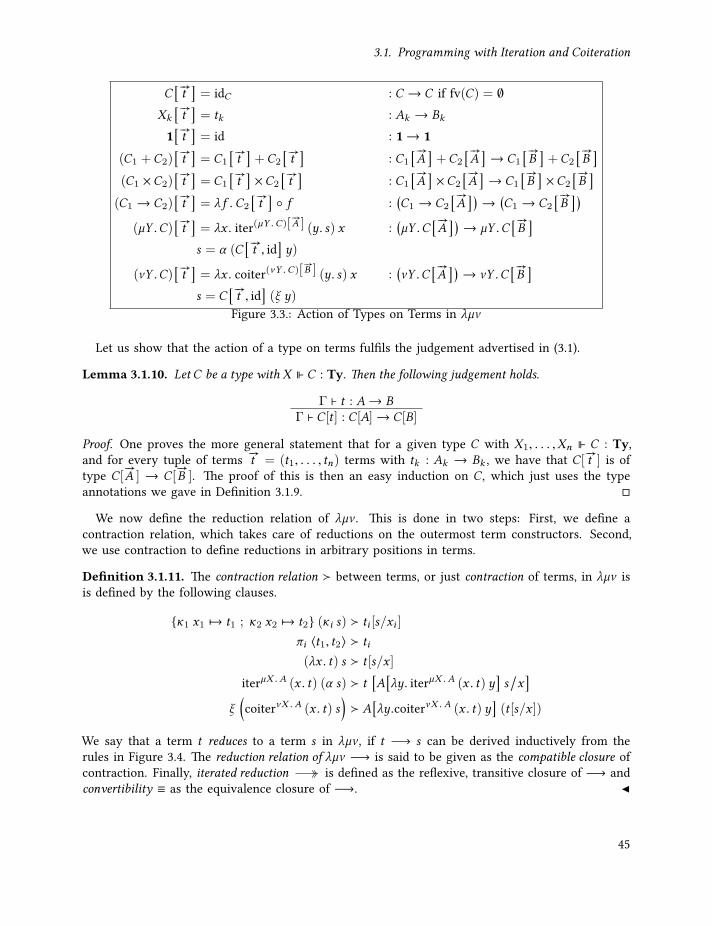
3.1. Programming with Iteration and Coiteration
C[
#—t]= idC : C → C if fv(C) = ∅
Xk[
#—t]= tk : Ak → Bk
1[
#—t]= id : 1→ 1
(C1 +C2)[
#—t]= C1
[#—t]+C2
[#—t]
: C1
[ #—A
]+C2
[ #—A
]→ C1
[ #—B
]+C2
[ #—B
](C1 ×C2)
[#—t]= C1
[#—t]×C2
[#—t]
: C1
[ #—A
]×C2
[ #—A
]→ C1
[ #—B
]×C2
[ #—B
](C1 → C2)
[#—t]= λ f .C2
[#—t] f :
(C1 → C2
[ #—A
] )→
(C1 → C2
[ #—B
] )(µY .C)
[#—t]= λx . iter(µY .C)[
#—A ] (y. s) x :
(µY .C
[ #—A
] )→ µY .C
[ #—B
]s = α (C
[#—t , id
]y)
(νY .C)[
#—t]= λx . coiter(νY .C)[
#—B ] (y. s) x :
(νY .C
[ #—A
] )→ νY .C
[ #—B
]s = C
[#—t , id
](ξ y)
Figure 3.3.: Action of Types on Terms in λµν
Let us show that the action of a type on terms fulfils the judgement advertised in (3.1).
Lemma 3.1.10. Let C be a type with X ⊩ C : Ty. Then the following judgement holds.
Γ ⊢ t : A→ BΓ ⊢ C[t ] : C[A]→ C[B]
Proof. One proves the more general statement that for a given type C with X1, . . . ,Xn ⊩ C : Ty,and for every tuple of terms #—
t = (t1, . . . , tn) terms with tk : Ak → Bk , we have that C[ #—t ] is of
type C[#—A ] → C[
#—B ]. The proof of this is then an easy induction on C , which just uses the type
annotations we gave in Definition 3.1.9.
We now define the reduction relation of λµν . This is done in two steps: First, we define acontraction relation, which takes care of reductions on the outermost term constructors. Second,we use contraction to define reductions in arbitrary positions in terms.
Definition 3.1.11. The contraction relation ≻ between terms, or just contraction of terms, in λµν isis defined by the following clauses.
κ1 x1 7→ t1 ; κ2 x2 7→ t2 (κi s) ≻ ti [s/xi ]
πi ⟨t1, t2⟩ ≻ ti
(λx . t) s ≻ t [s/x ]
iterµX .A (x . t) (α s) ≻ t[A[λy. iterµX .A (x . t) y
]s/x]
ξ(coiterνX .A (x . t) s
)≻ A
[λy.coiterνX .A (x . t) y
](t [s/x ])
We say that a term t reduces to a term s in λµν , if t −→ s can be derived inductively from therules in Figure 3.4. The reduction relation of λµν −→ is said to be given as the compatible closure ofcontraction. Finally, iterated reduction is defined as the reflexive, transitive closure of −→ andconvertibility ≡ as the equivalence closure of −→.
45

Chapter 3. Inductive-Coinductive Programming
t ≻ st −→ s
t −→ sπi t −→ πi s
t −→ t ′
⟨t , s⟩ −→ ⟨t ′, s⟩s −→ s ′
⟨t , s⟩ −→ ⟨t , s ′⟩t −→ t ′
t s −→ t ′ ss −→ s ′
t s −→ t s ′
t −→ sλx . t −→ λx . s
s −→ s ′
κ1 x 7→ s ; κ2 y 7→ t u −→ κ1 x 7→ s ′ ; κ2 y 7→ t ut −→ t ′
κi t −→ κi t′
t −→ t ′
κ1 x 7→ s ; κ2 y 7→ t u −→ κ1 x 7→ s ; κ2 y 7→ t ′ ut −→ t ′
α t −→ α t ′t −→ t ′
ξ t −→ ξ t ′u −→ u ′
κ1 x 7→ s ; κ2 y 7→ t u −→ κ1 x 7→ s ; κ2 y 7→ t u ′t −→ t ′
(co)iter (x . t) s −→ (co)iter (x . t ′) ss −→ s ′
(co)iter (x . t) s −→ (co)iter (x . t) s ′
Figure 3.4.: Compatible Closure of Contraction in λµν
Let us illustrate the reduction relation by means of addition on natural numbers and streams.
Example 3.1.12. We show that addition of natural numbers, defined in Example 3.1.7, has theexpected computational behaviour on zero and successors. For C = 1 + X , we have for any termsu and t the following.
C[u] t = (1[u] + X [u]) t
= (id1 + u) t
= (λx . κ1 y 7→ κ1 (id1 y) ; κ2 z 7→ κ2 (u z) x) t≻ κ1 y 7→ κ1 (id1 y) ; κ2 z 7→ κ2 (u z) t−→ κ1 y 7→ κ1 y ; κ2 z 7→ κ2 (u z) t by id1 y ≻ y
(3.2)
Recall that д+ was defined in Example 3.1.7 by д+ = λm. κ1 y 7→ m ; κ2 f 7→ suc (f m) x .Using this and (3.2), we get for any term t of type Nat that 0 + t t and hence 0 + t ≡ t bythe sequence of reduction steps in Figure 3.5, where we use R B λy. iter (x .д+) y as a short-handnotation. Similarly, we get for s : Nat the reduction sequence in Figure 3.6. Now we note that
suc (iterNat (x .д+) s t)←− suc ((λnm. iterNat (x .д+) nm) s t) = suc (s + t),
so that (suc s) + t ≡ suc (s + t) as expected.12
Example 3.1.13. Similarly to the last example, we demonstrate that the terms given in Example 3.1.8have the expected computational behaviour. For the constant streams we have
hd aω = hd (coiter дa ⟨ ⟩) ≡ π1 ((id × (coiter дa)) (дa ⟨ ⟩))≡ π1 ((id × (coiter дa)) ⟨a, ⟨ ⟩⟩)≡ π1 ⟨a, (coiter дa ⟨ ⟩)⟩≡ a,
andtl aω = tl (coiter дa ⟨ ⟩) ≡ · · · ≡ π2 ⟨a, (coiter дa ⟨ ⟩)⟩ ≡ coiter дa ⟨ ⟩ = aω .
46

3.1. Programming with Iteration and Coiteration
0 + t
= (λnm. iterNat (x .д+) nm) 0 t
≻ (λm. iterNat (x .д+) 0m) t
≻ iterNat (x .д+) 0 t
= iterNat (x .д+) (α (κ1 ⟨ ⟩)) t
−→ д+ [C[R] (κ1 ⟨ ⟩)/x ] t iterNat (x .д+) (α (κ1 ⟨ ⟩)) ≻ . . .−→ д+[κ1 y 7→ κ1 y ; κ2 z 7→ κ2 (R z) (κ1 ⟨ ⟩)/x ] t by (3.2)−→ д+[κ1 ⟨ ⟩/x ] t κ1 x 7→ κ1 x ; · · · (κ1 ⟨ ⟩) ≻ κ1 ⟨ ⟩=
(λm. κ1 y 7→m ; κ2 f 7→ suc (f m) (κ1 ⟨ ⟩)
)t
≻ κ1 y 7→ t ; κ2 f 7→ suc (f t) (κ1 ⟨ ⟩)≻ t
Figure 3.5.: Reduction Sequence for 0 + t in λµν
(suc s) + t = (λnm. iterNat (x .д+) nm) (α (κ2 s)) t
= · · ·−→ д+[κ1 y 7→ κ1 y ; κ2 z 7→ κ2 (iterNat (x .д+) z) (κ2 s)/x ] t−→ д+ [κ2 (iterNat (x .д+) s)/x ] t
=(λm. κ1 y 7→m ; κ2 f 7→ suc (f m) (κ2 (iterNat (x .д+) s))
)t
≻ κ1 y 7→ t ; κ2 f 7→ suc (f t) (κ2 (iterNat (x .д+) s))
≻ suc (iterNat (x .д+) s t)
Figure 3.6.: Reduction Sequence for (suc s) + t in λµν
An easy calculation also shows that
hd (s ⊕ t) ≡ hd s + hd t and tl (s ⊕ t) ≡ tl s ⊕ tl t .
We can use these equivalences now to check the computational behaviour of the second definitionof the stream of natural numbers:
hd nats2 = hd (coiter д2 0ω) ≡ π1 ((id × coiter д2)(д2 0ω))≡ π1 ((id × coiter д2)(hd 0ω , 0ω ⊕ 1ω)) ≡ 0.
Note that we can continue to explicitly check that the n-th position of nats2, given by hd (tln nats2),is indeed n. We introduce in Chapter 5 the necessary machinery to prove this for all n.
Let us now show that the reduction relation preserves types of terms, that is, if Γ ⊢ t : A andt −→ s , then Γ ⊢ s : A. We say then that subject reduction holds for −→. The first step towards thiswas Lemma 3.1.10, where we proved that the type action is type correct, which allows us to provesubject reduction for the contraction relation introduced in Definition 3.1.11. This, in turn, givesimmediately that the reduction relation preserves types by its definition as compatible closure ofcontraction.
47

Chapter 3. Inductive-Coinductive Programming
Theorem 3.1.14. The reduction relation of λµν preserves types.
Proof. We first show that the contraction relation preserves types. The cases for sum types, productand function types are readily proved by a standard argument. For the contraction on recursivetypes, we use Lemma 3.1.10 as follows. Suppose we have Γ,x : A[B/X ] ⊢ t : B and Γ ⊢ s : A[µX .A/X ],so that Γ ⊢ iterµX .A (x . t) (α s) : B. The following derivation then shows that the right-hand side ofthe contraction for iteration also has type B.
Γ ⊢ λy. iterµX .A (x . t) y : (µX .A)→ B
Γ ⊢ A[λy. iterµX .A (x . t) y
]: A[µX .A]→ A[B] Γ ⊢ s : A[µX .A/X ]
Γ ⊢ A[λy. iterµX .A (x . t) y
]s : A[B]
Γ ⊢ t [A[λy. iterµX .A (x . t) y
]s/x ] : B
Similarly, for t : A[B/X ] and s : B, we have that in the case of ν-types the type of the right side ofthe contraction matches that of the left side. This is demonstrated by the following type derivation.
Γ ⊢ λy. coiterνX .A (x . t) y : B → νX .A
Γ ⊢ A[λy. coiterνX .A (x . t) y
]: A[B]→ A[νX .A]
Γ ⊢ s : BΓ ⊢ t [s/x ] : A[B]
Γ ⊢ A[λy. coiterνX .A (x . t) y
](t [s/x ]) : A[νX .A]
Second, since the contraction relation preserves types and the reduction relation is the compatibleclosure of contraction, type preservation of reductions is immediate.
This concludes our introduction into simple inductive-coinductive programming, and we move onto a more practical language.13
3.2. Programming with EquationsIn the previous section, we have introduced the simply typed calculus λµν for programming withmixed inductive-coinductive types. It was fairly straightforward to set up the calculus and, as notedin Note 13, all terms of that calculus are strongly normalising. However, since the calculus is basedon iteration and coiteration schemes, programming can become quite complicated. We have seenthis already in Example 3.1.7, but the complications become even more prevalent when iteration andcoiteration are mixed.
For example, suppose we want to define a map that projects a left-fair stream to its A-elements.In λµν we can define such a map as follows.
Example 3.2.1. To define the projection proj : LFairAB → Aω , we put U = A× (LFairAB) + B ×Yand let L = µY .U be the first unfolding of LFair. Then we define
proj = λx . coiterAω f x
f : LFairA B → A × LFairA B
f x = iterL д (ξ x)д : U [A × LFairA B/Y ]→ A × LFairA B
д x = κ1 x 7→ x ; κ2 y 7→ π2 y x
48

3.2. Programming with Equations
This is a short definition, but coming up with it, let alone understanding it, is rather difficult.
This situation can be improved by moving away from (co)iteration schemes and instead useequational specifications, which allow recursive references to function symbols. This is essentiallyhow one writes programs in a functional language like Haskell. We will introduce in this section acalculus, denoted by λµν=, that implements this idea by replacing the (co)iteration schemes of λµνby recursive equations, patterns and so-called copatterns. This calculus is a variation of the copatterncalculus given by Abel et al. [Abe+13] . We discuss the differences and rationale for these changesin Section 3.4. The calculus λµν= has been studied in [BH16]. Note, however, that in loc. cit. thesyntax is slightly different, in that the authors use a syntax similar to that of λµν for destructorsof products and ν-types. The choice of syntax in this section brings the calculus λµν= closer tobehavioural differential equations [Rut03], object oriented programming and the original syntaxin [Abe+13]. It also emphasises that function space types are coinductive, in that its destructor, thefunction application, is also written in post-fix notation.
3.2.1. Types and Terms of the Calculus λµν=The types for the calculus λµν= are exactly the ones we gave in Definition 3.1.1 for λµν . As for theterms, the introduction rules for coproducts and µ-types are the same, whereas the elimination rulesfor coinductive types (products, functions and ν-types) are now all written in post-fix notation. Also,the elimination rules for inductive types (sums and µ-types) and introduction rules for coinductivetypes will be replaced by patterns and copatterns, respectively, combined with recursive equations.Such recursive equations can thereby be given via a binding construct rletΣ in t , where Σ containssymbols and their definitions, and t is a term. The calculus is formally given by the followingdefinition.
Definition 3.2.2. Let TeVar and SigVar be countably infinite, disjoint sets of term variables x ,y, z, . . .and signature variables f ,д,h, . . ., respectively. The raw terms s, t , patterns p, copatterns q, declarationbodies D and declaration blocks Σ of λµν= are generated by the following grammar.
s, t F x ∈ TeVar | ⟨ ⟩ | κ1 t | κ2 t | α t | t .pr1 | t .pr2 | t .out | t s| f ∈ SigVar | λD | rlet Σ in t
p F x ∈ TeVar | κi p | α p
q F · | q.pr1 | q.pr2 | q.out | q pD F q1 7→ t1 ; . . . ; qn 7→ tnΣF f1 : A1 = D1, . . . , fn : An = Dn
To resolve ambiguities, To increase readability, we adopt here the same conventions as for λµν(application is left-associative and variables do not need parentheses) plus that application of de-structors is also left-associative. For example, t .out.pr1 is to be read as (t .out).pr1. The analogousconventions also hold for patterns and copatterns.
We now define what the (well-typed) terms of λµν= are.
Definition 3.2.3. A context Γ is a possibly empty sequence x1 : A1, . . . ,xn : An of variablesxi ∈ TeVar annotated with types Ai . A raw term t is said to be a term of λµν= of type A in context
49

Chapter 3. Inductive-Coinductive Programming
Γ using the declarations in Σ, if Γ;Σ ⊢ t : A can be derived inductively from the rules in Fig. 3.7. Wedenote the set of all well-typed terms by Termsλµν=. The judgement for well-typed terms involvesthe following judgements, which are defined in Fig. 3.7 as well.
• Γ;Σ ⊢bdy D : A, states that D is a declaration body of type A in the variable context Γ usingthe declarations in Σ;
• Σ1 ⊢dec Σ2, states that Σ2 is a well-formed declaration block, using declarations in Σ1;
• Γ ⊢pat p : A, states that p is a pattern on the type A that binds variables in Γ; and
• Γ ⊢cop q : A⇒ B, states that q is a copattern, binding variables in Γ, such that for all evaluationcontexts e that match q, applying e to a term of type A results in a term of type B.
(x : A) ∈ Γ(Proj)
Γ;Σ ⊢ x : A
(f : A = D) ∈ Σ(ProjSig)
Γ;Σ ⊢ f : A(1-I)
Γ;Σ ⊢ ⟨ ⟩ : 1
Γ;Σ ⊢ t : Ai(i = 1, 2) (+-I)
Γ;Σ ⊢ κi t : A1 +A2
Γ;Σ ⊢ t : A[µX .A/X ](µ-I)
Γ;Σ ⊢ α t : µX .A
Γ;Σ ⊢ t : A1 ×A2 (×-E1)Γ;Σ ⊢ t .pr1 : A1
Γ;Σ ⊢ t : A1 ×A2 (×-E2)Γ;Σ ⊢ t .pr2 : A2
Γ;Σ ⊢ t : νX .A (ν-E)Γ;Σ ⊢ t .out : A[νX .A/X ]
Γ; Σ ⊢ t1 : A→ B Γ;Σ ⊢ t2 : A (→-E)Γ;Σ ⊢ t1 t2 : B
Γ;Σ ⊢bdy D : A(Abs)
Γ;Σ ⊢ λD : A
Σ1 ⊢dec Σ2 Γ;Σ1,Σ2 ⊢ t : A (Rlet)Γ;Σ1 ⊢ rlet Σ2 in t : A
Γi ⊢cop qi : B ⇒ Ai Γ,Γi ; Σ ⊢ ti : Ai for all 1 ≤ i ≤ n
Γ;Σ ⊢bdy q1 7→ t1; . . . ;qn 7→ tn : B
∅; Σ1,Σ2 ⊢bdy D : A for all (f : A = D) ∈ Σ2
Σ1 ⊢dec Σ2
x ∈ Varx : D ⊢pat x : D ⊢pat ⟨ ⟩ : 1
x : D ⊢pat p : Ai
x : D ⊢pat κi p : A1 +A2
x : D ⊢pat p : A[µX .A/X ]
x : D ⊢pat α p : µX .A
∅ ⊢cop · : C ⇒ C
Γ ⊢cop q : C ⇒ A1 ×A2
Γ ⊢cop q.pr1 : C ⇒ A1
Γ ⊢cop q : C ⇒ A1 ×A2
Γ ⊢cop q.pr2 : C ⇒ A2
Γ ⊢cop q : C ⇒ νX .A
Γ ⊢cop q.out : C ⇒ A[νX .A/X ]
Γ ⊢cop q : C ⇒ (A→ B) x : D ⊢pat p : A x < ΓΓ,x : D ⊢cop q p : C ⇒ B
Figure 3.7.: Rules for forming terms, declaration bodies and blocks, and (co)patterns
50

3.2. Programming with Equations
Let us explain the typing rules in Definition 3.2.3. The main difference with the calculus λµνis that we omit the iteration and coiteration schemes in favour of rlet-blocks. Such blocks allowus to construct terms with recursive occurrences of symbols, that is, in a term rlet Σ2 in t , thesymbols defined in the declaration block Σ2 can be (directly or indirectly) self-referential. This canbe seen from the single rule for Σ1 ⊢dec Σ2 in Figure 3.7, where every declaration body in Σ2 ischecked with all declarations of Σ2 in scope. Note that there is no restriction on the recursiveoccurrence of symbols, which means that it is possible to write non-terminating programs in λµν=,see Example 3.2.21. On the other hand, this also allows us to write programs that are well-definedbut not obeying any syntactic restriction like guardedness [Gim95], see Example 4.1.6.
The declaration bodies form the heart of the calculus, as they allow us to define objects ofcoinductive type by means of copatterns and functions out of inductive types by means of patterns.For instance, to define a function of type A+ B → C , we may use pattern matching to distinguishwhether we get an element from A or B as input. Given terms s and t of type C , we can form thedeclaration body D with D =
· (κ1 x) 7→ s ; · (κ2 y) 7→ t
, which covers the two cases of the sum
type. We may then use the abstraction rule to form the term λD of type A + B → C that allowsus to carry out the case distinction, see Example 3.2.4. Concerning coinductive types, we insteadspecify the outcome of observations that can be made on a term through the use of destructors. Forexample, given terms s and t respectively of type A and B, we can obtain the pair of these termsby abstraction of the declaration body D defined by D =
· .pr1 7→ s ; · .pr2 7→ t
, which gives us
λD : A × B. Pairing for products is further explained in Example 3.2.5. The last example that wediscuss at this point are streams. To increase readability, we introduce some short-hand notationsfor head and tail projections on streams:
.hd B .out.pr1 and .tl B .out.pr2. (3.3)
As one would expect, a stream is given by providing the terms for the head and tail, say s : A andt : Aω , and bundling them in the body
· .hd 7→ s ; · .tl 7→ t : A ×Aω .
We will see in Example 3.2.9, Example 3.2.10 and Example 3.2.11 further specifications of streams.Let us now explain patterns and copatterns in more broad terms. As we said above, copatterns
allow us to specify the outcome of observations on a term, while patterns allow us to analysearguments of inductive type. This idea is reflected in the interplay of the typing rules for declarationbodies, patterns and copatterns. Generally, the judgement Γ ⊢cop q : C ⇒ B says that if we want toform a declaration body of the form q 7→ t of type C , then t must be of type B and the abstractionλq 7→ t binds all the variables in Γ. Consider, for instance, the declaration body D =
· (α x) 7→ t
.
First of all, we expect that λD is a function that takes an argument of type µX .A for some type Aand returns something of type B. Second, λD should bind the variable x in t . Both requirements areincluded in the typing of the copattern · (αx), which in turn is obtained by the following derivation.
∅ ⊢cop · :((µX .A)→ B
)⇒
((µX .A)→ B
) x : A[µX .A/X ] ⊢pat x : A[µX .A/X ]
x : A[µX .A/X ] ⊢pat α x : µX .A
x : A[µX .A/X ] ⊢cop · (α x) :((µX .A)→ B
)⇒ B
We can now read off from this that t can have a free variable of type A[µX .A/X ], which is boundin λD, that t must be of type B, and that the type of λD is then (µX .A) → B. In the course of
51

Chapter 3. Inductive-Coinductive Programming
the examples below, we will familiarise ourselves more with this interplay between the rules forcopatterns and declaration bodies.
There are two aspects of declarations that are worthwhile to discuss. First, we mentioned alreadythat the variables contained in copatterns are bound through declaration bodies. To avoid dependen-cies between patterns in a body and the problems that spring from such dependencies, one usuallyrequires patterns of a declaration to be linear , that is, variables may occur at most once in them.We ensure this here in the rule for copatterns of function application by checking, upon formingthe copattern q p, that the variable that appears in the argument pattern p does not occur already inthe copattern q. This guarantees that any variable occurs at most once in a copattern, which rulesout copatterns like “· (κ1 x) x”. Second, the reader might have noticed that neither the definitionof raw terms nor that of well-typed terms ensures that a declaration body has to cover all cases.Consider for instance the term f given by f = λ
· (κ1 x) 7→ t
, which does not cover the case that
an argument may be of the form κ2 s . Thus, if we tried to evaluate f (κ2 s), then the computa-tion would get stuck. So far, there is nothing in the calculus that ensures that a declaration bodycovers all possible cases for (co)patterns. It even might happen that there are several cases for thesame copattern, which would make computations non-deterministic. We will discuss this further inExample 3.2.23 and then address these issues when proving confluence in Proposition 3.2.32.
Let us now go through the remaining rules in Figure 3.7. We have already seen that (Rlet) allowsus to construct terms with recursively defined symbols. The rule (ProjSig) complements this, inthat it allows us to use any declared symbol as term. Sometimes, we would like to give a term inthe form of a declaration body without having to introduce a new symbol, see Example 3.2.5 below.This can be done by using the rule (Abs). The other rules to construct terms correspond exactly tothose in λµν , except that the destructors appear in post-fix position.
We illustrate λµν= on some non-recursive examples, in which we recover notations from λµν . InSection 3.3, we will properly study the relation between these two calculi.
Example 3.2.4. We have almost the same notation for case distinction on sums:
κ1 x 7→ s ; κ2 y 7→ t u B λ· (κ1 x) 7→ s ; · (κ2 y) 7→ t
u
Let us check that this definition is well-typed. The first step is to assign types to the two copatternsin the term on the right. This is done by the following two derivations.
⊢cop · : (A+ B → C)⇒ (A+ B → C)
x : A ⊢pat x : A
x : A ⊢pat κ1 x : A+ B
x : A ⊢cop · (κ1 x) : (A+ B → C)⇒ C
⊢cop · : (A+ B → C)⇒ (A+ B → C)
y : B ⊢pat y : B
y : B ⊢pat κ2 y : A+ B
y : B ⊢cop · (κ2 y) : (A+ B → C)⇒ C
Next, we check the type of the abstraction. For this, suppose that we have Γ,x : A ⊢ s : C andΓ,y : B ⊢ t : C and Γ;Σ ⊢ u : A+ B. Using the short-hand notation U = A+ B → C , we can make
52

3.2. Programming with Equations
the following derivation.
x : A ⊢cop · (κ1 x) : U ⇒ C
y : B ⊢cop · (κ2 y) : U ⇒ C Γ,x : A ⊢ s : C Γ,y : B ⊢ t : CΓ;Σ ⊢bdy
· (κ1 x) 7→ s ; · (κ2 y) 7→ t
: A+ B → C
Γ;Σ ⊢ λ· (κ1 x) 7→ s ; · (κ2 y) 7→ t
: A+ B → C
Finally, we check the application to u:
Γ;Σ ⊢ λ· (κ1 x) 7→ s ; · (κ2 y) 7→ t
: A+ B → C Γ;Σ ⊢ u : A+ B
Γ;Σ ⊢ λ· (κ1 x) 7→ s ; · (κ2 y) 7→ t
u : C
Thus the definition of case distinction we gave above is well-typed.
Next, we can also recover the notation for product types that we used in λµν .
Example 3.2.5. The projections on product types can be defined for u : A × B by
π1 u B u .pr1 and π2 u B u .pr2,
so that the pairing constructor is given by
⟨s, t⟩ B λ· .pr1 7→ s ; · .pr2 7→ t
.
Let us again check that these definitions are well-typed. This is clear for the projections, so wecheck just the pairing. Assume that Γ;Σ ⊢ s : A and Γ;Σ ⊢ t : B. Then we have
⊢cop · : A × B ⇒ A × B⊢cop · .pr1 : A × B ⇒ A
⊢cop · : A × B ⇒ A × B⊢cop · .pr2 : A × B ⇒ B
Γ;Σ ⊢bdy· .pr1 7→ s ; · .pr2 7→ t
: A × B
Γ;Σ ⊢ λ· .pr1 7→ s ; · .pr2 7→ t
: A × B
as required.
Finally, we can also recover the usual notation for function spaces.
Example 3.2.6. Note that application of terms of function type is written in λµν= just as in λµν .However, λ-abstraction is slightly more complicated:
λx . t B λ· x 7→ t.
Assuming that Γ,x : A; Σ ⊢ t : B, we can indeed derive the following.
⊢cop · : (A→ B)⇒ (A→ B)
⊢cop · x : (A→ B)⇒ B Γ,x : A; Σ ⊢ t : BΓ;Σ ⊢bdy · x 7→ t : A→ B
Γ;Σ ⊢ λ· x 7→ t : A→ B
So the λ-abstraction is well-typed with the expected type.
53

Chapter 3. Inductive-Coinductive Programming
Recall from Example 3.1.6 that we could represent in λµν a one-element set by the fixed pointtype νX .X . This is again true in λµν=, except that the inhabitant ⟨ ⟩′ is easier to establish.
Example 3.2.7. Recall from Example 3.1.6 that we used the coiteration scheme of λµν on a functiontype to get an inhabitant of the type 1′. In λµν= this inhabitant can be given much easier by
⟨ ⟩′ B rlet f : 1′ = · .out 7→ f in f .
Let us use the typing rules to show that ⟨ ⟩′ : 1′ indeed holds.
⊢cop · : 1′⇒ 1′
⊢cop · .out : 1′⇒ X [1′/X ] f : 1′ ⊢ f : 1′
f : 1′ ⊢bdy · .out 7→ f : 1′
⊢dec f : 1′ = · .out 7→ f f : 1′ ⊢ f : 1′
⊢ ⟨ ⟩′ : 1′
In Section 4.1, it will turn out that also this inhabitant of 1′ is canonical.
We have advertised the present calculus as being easier to program with. The next exampledemonstrates this on the projection out of the left-fair streams. Since these streams are given by amixed inductive-coinductive type, the example combines patterns and copatterns.
Example 3.2.8. Recall the type LFair A B = νX . µY . (A × X + B × Y ), consisting of streams overA and B, such that elements of A occur infinitely often. We define a map that projects a left-fairstream onto a stream over A as in Example 3.2.1. This can be done by defining maps pA and eraseBby mutual recursion as follows.
projA B rletpA : LFairA B → Aω =
(· x).out 7→ eraseB (x .out)
eraseB : µY . (A × LFairA B) + B × Y )→ A ×Aω = · (α (κ1 u)) 7→ ⟨u .pr1, pA (u .pr2)⟩ ;· (α (κ2 u)) 7→ eraseB (u .pr2)
in pA
Note that pA is defined coinductively, whereas eraseB is defined by induction.We now derive the type of projA. For brevity, let us agree on the following short-hand notation.
F = LFairA B L = µY . (A × LFairA B) + B × Y )V = F → Aω W = L→ A ×Aω
Σ = pA : V , eraseB :W
First, we find that the type of the copattern used in pA is V ⇒ A ×Aω :⊢cop · : V ⇒ V u : F ⊢pat u : F
u : F ⊢cop · u : V ⇒ Aω
u : F ⊢cop (· u).out : V ⇒ A ×Aω(3.4)
54

3.2. Programming with Equations
We can use this information then to check that the body of pA is type-correct:
(3.4)u : F ; Σ ⊢ eraseB :W
u : F ; Σ ⊢ u : F
u : F ; Σ ⊢ u .out : Lu : F ; Σ ⊢ eraseB(u .out) : A ×Aω
Σ ⊢bdy(· u).out 7→ eraseB (u .out)
: V
Similarly, we can type the body of eraseB . Putting these two derivations together, we can checkthat Σ is well-formed.
...
Σ ⊢bdy(· u).out 7→ . . .
: V
...
Σ ⊢bdy· (α(κ1 v)) 7→ . . .
:W
⊢dec Σ (3.5)
Finally, we check the rlet-declaration that defines projA:
(3.5) Σ ⊢ pA : V
⊢ projA : LFairA B → Aω
Thus projA is a well-formed term.Note that projA is defined by a single rlet-block, which declares a fresh symbol pA that defines
projA. Since this situation occurs quite frequently, we will usually leave out this rlet and presentits content as a set of equations, just like one would write programs in Haskell or how behaviouraldifferential equations are given. The above program is then given as follows.
projA : LFairA B → Aω
(projA x).out = eraseB (x .out)eraseB : µY . (A × LFairA B) + B × Y )→ A ×Aω
eraseB (α (κ1 y)) = ⟨y.pr1, projA (y.pr2)⟩eraseB (α (κ2 y)) = eraseB (y.pr2)
This lifts some notational burden and makes programs easier to read.
The next example demonstrates the use of mixed induction-coinduction on streams over naturalnumbers. Note that, in contrast to left-fair streams, this is a type in which least and greatest fixedpoint types are separable but the function still mixes induction and coinduction.
Example 3.2.9. We define a function H of type Natω → Natω → Natω that maps streams s and t toa stream r with r(n) = t(
∑ni=0 s(i)) by mixing patterns and copatterns as in the following program.
We display the program in two forms: on the left in the formally correct notation of λµν= and onthe right in the more readable, Haskell-like notation that we introduced in Example 3.2.8.
55
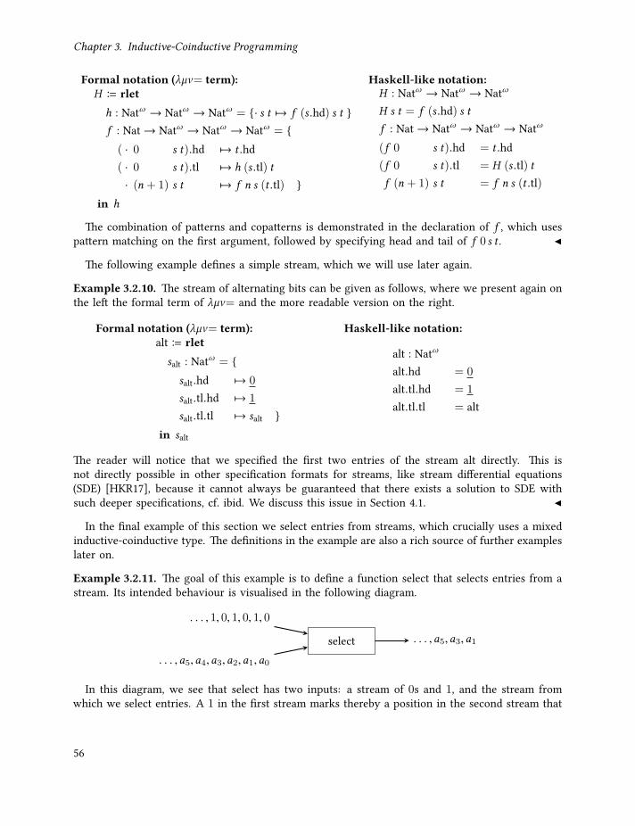
Chapter 3. Inductive-Coinductive Programming
Formal notation (λµν= term):H B rleth : Natω → Natω → Natω = · s t 7→ f (s .hd) s t f : Nat→ Natω → Natω → Natω = ( · 0 s t).hd 7→ t .hd( · 0 s t).tl 7→ h (s .tl) t· (n + 1) s t 7→ f n s (t .tl)
in h
Haskell-like notation:H : Natω → Natω → Natω
H s t = f (s .hd) s tf : Nat→ Natω → Natω → Natω
(f 0 s t).hd = t .hd(f 0 s t).tl = H (s .tl) tf (n + 1) s t = f n s (t .tl)
The combination of patterns and copatterns is demonstrated in the declaration of f , which usespattern matching on the first argument, followed by specifying head and tail of f 0 s t .
The following example defines a simple stream, which we will use later again.
Example 3.2.10. The stream of alternating bits can be given as follows, where we present again onthe left the formal term of λµν= and the more readable version on the right.
Formal notation (λµν= term):alt B rletsalt : Natω = salt.hd 7→ 0
salt.tl.hd 7→ 1
salt.tl.tl 7→ salt in salt
Haskell-like notation:
alt : Natω
alt.hd = 0
alt.tl.hd = 1
alt.tl.tl = alt
The reader will notice that we specified the first two entries of the stream alt directly. This isnot directly possible in other specification formats for streams, like stream differential equations(SDE) [HKR17], because it cannot always be guaranteed that there exists a solution to SDE withsuch deeper specifications, cf. ibid. We discuss this issue in Section 4.1.
In the final example of this section we select entries from streams, which crucially uses a mixedinductive-coinductive type. The definitions in the example are also a rich source of further exampleslater on.
Example 3.2.11. The goal of this example is to define a function select that selects entries from astream. Its intended behaviour is visualised in the following diagram.
select
. . . , 1, 0, 1, 0, 1, 0
. . . ,a5,a4,a3,a2,a1,a0
. . . ,a5,a3,a1
In this diagram, we see that select has two inputs: a stream of 0s and 1, and the stream fromwhich we select entries. A 1 in the first stream marks thereby a position in the second stream that
56

3.2. Programming with Equations
should be kept, whereas 0s mark positions that shall be dropped. However, there is a problem if thefirst stream consists only of 0s, as we would have to drop all entries of the second input and thuswould not be able to compute an output stream.
This problem is solved, if we only accept streams that contain infinitely many 1s or, equivalently,in which all consecutive sequences of 0s are finite. We can guarantee this property by using streamselectors instead of 0-1-streams, which are elements of the following type F .
F B νX . µY .X + Y
Fµ B µY . F + Y
Let us give some names to the constructors of Fµ to improve readability. For patterns Γ1 ⊢pat p1 : Fand Γ2 ⊢pat p2 : Fµ , we define the following patterns for the type Fµ .
pres p1 B α (κ1 p1)
drop p2 B α (κ2 p2)
The first pattern signifies that an entry should be preserved, which corresponds to a 1 in the intuitiveexplanation of selectors above. On the other hand, we mark positions that shall be dropped by thesecond pattern, the 0 in the bit sequence view. Using these notations, we can implement the selectfunction, mutually with an auxiliary function on Fµ , as follows.
select : F → Aω → Aω
select x = selectµ (x .out)selectµ : Fµ → Aω → Aω
(selectµ (pres x) s).hd = s .hd(selectµ (pres x) s).tl = select x (s .tl)selectµ (drop u) s = selectµ u (s .tl)
The functions select and selectµ are typical examples of a mixed inductive-coinductive definition:We define selectµ by induction on the first argument, and by coinduction in the base case pres x ofthis induction. The role of select is to unfold the selector one step, so that we can calculate the nextelement of the output stream.
Let us now also use the same notation for constructing elements of Fµ as we did for the patterns.That is, given an element x of type F , we write pres x B α (κ1 x) : Fµ and similar for drop. Thisallows us to concisely give a selector for the odd positions of a stream as follows.
oddF : F
oddF.out = drop (pres oddF)
Intuitively, this selector corresponds to the stream (0, 1, 0, 1, 0, 1 . . . ) in the original picture. It allowsus to define the following function that drops all the even positions of streams over A.
odd : Aω → Aω
odd = select oddF
57

Chapter 3. Inductive-Coinductive Programming
We will see in Example 3.2.19 the computational behaviour of select. In Chapter 5 we will be ableto show that select indeed produces an output for any selector, and in the same chapter we provesome further properties of select. Finally, in Chapter 7 we apply selectors and the select function inthe proof of a proposition.
Let us discuss some interesting aspects of Example 3.2.11. First, Bertot [Ber05] uses selection fromstreams by means of predicates to implement the sieve of Eratosthenes in Coq. Suppose that A is atype, P a predicate14 on A and s : Aω a stream on A. Bertot then aims to define a stream select P sthat arises from s by keeping exactly those entries that fulfil the predicate P . However, it is clearthat such a stream does not exist for all combinations of predicates and streams, but only if thepredicate P holds on infinitely many entries of the stream s . If we say in this situation that P is fairon s , then we can alternatively describe this fairness property as inductive-coinductive property: Pis fair on s if P eventually holds on some element in s and P is fair on the stream after that position.We will make this definition precise in Section 7.5.3. Let us just say that this fairness of P on scorresponds to the formula ^P (read: always, eventually P ) in linear temporal logic. In contrastto Bertot’s development, we have selected entries from streams in Example 3.2.11 by specifying thepositions that should be kept/dropped from a stream, so that a selector is independent of the streamfrom which we select. However, these two approaches of selecting can be seen to be equivalent.
The second interesting aspect of entry selection is its relation to (uniform) continuity. Let us writes ≈n t for n ∈ N and stream terms s, t : Aω , if s and t agree on the first n entries. More precisely,
s ≈n t B ∀k < n. (s .tlk .hd ≡ t .tlk .hd),
where .tlk is the k-fold application of .tl. This gives us a metric on stream terms [Smy92, Chap. 6]:
d(s, t) = inf2−n | n ∈ N, s ≈n t.
A term f : Aω → Aω is uniformly continuous with modulus of continuity M : N→ N, if for all n ∈ N
∀s, t : Aω .d(s, t) ≤ 2−M(n) =⇒ d(f s, f t) ≤ 2−n .
Note now that for a stream s the n-th element of odd s is the (2n+1)-th element of the input streams . Thus, we claim that odd is uniformly continuous with modulus M(n) = 2n + 1. Indeed, we candefine a map mod : F → Nat→ Nat that computes for x : F the modulus of continuity of select x :
mod x = modµ (x .out)modµ : Fµ → Nat→ Natmodµ (pres x) 0 = 0
modµ (pres x) (suc n) = suc (mod x n)modµ (drop x) n = suc (modµ x n)
In Example 3.2.20, we show that mod oddF n computes 2n + 1. This will allow us to show that thelook-ahead of odd, that is, the number of entries that are read from an input to produce an output,is bounded by mod oddF. In other words, odd is uniformly continuous with modulus mod oddF.15
58

3.2. Programming with Equations
3.2.2. Computations in λµν=We now give a reduction relation on terms in λµν=. This reduction relation has at its heart again acontraction relation, which essentially applies the defining equations as rewrite rules. For instance,we will have
⟨ ⟩′.out = (rlet f : 1′ = · .out 7→ f in f ).out−→ rlet f : 1′ = · .out 7→ f in (f .out)−→ rlet f : 1′ = · .out 7→ f in f
= ⟨ ⟩′.
Turning copattern equations into rewrite rules also ensures that the definitions in Example 3.2.4,3.2.5 and 3.2.6 yield terms whose reductions coincide with their counterparts in λµν .
Definition 3.2.12. A substitution is a function σ : TeVar→ Termsλµν= that maps variables to terms.We denote by dom(σ) the domain of σ , which is given by dom(σ) = x | σ(x) , x. Given a termt ∈ Termsλµν=, the application t [σ ] of σ to t is the term that results from replacing all variablesx ∈ dom(σ) that are unbound in t by σ(x) while renaming bound variables in t (α-renaming) toavoid binding of variables in σ(x). For a context Γ, we denote by dom(Γ) the set of variables thatoccur in Γ. We then say that a substitution σ is a Γ-substitution, if dom(Γ) ⊆ dom(σ).
Definition 3.2.13. Given a copattern q with Γ ⊢cop q : A ⇒ B and a Γ-substitution σ , we calle = q[σ ] an evaluation context on type A with result in B and we say that q matches e . For terms t ,we denote by e[t/·] the term obtained by replacing the hole · in q[σ ] by t .
Note that in Definition 3.2.13, if there is a context Γ′, such that Γ′ ⊢ t : A and Γ′ ⊢ σ(x) : Γ(x)for all x ∈ dom(Γ), where Γ(x) is the type of the variable x in Γ, we have Γ′ ⊢ e[t/·] : B.
We use matching to define contraction and reductions of terms.
Definition 3.2.14. Given a term t : A and an evaluation context e , we say that the term e[t/·]contracts to t ′ using declarations in Σ, if e[t/·] ≻Σ t ′ can be derived using the following rules:
qi 7→ ti ∈ Dqi [σ ][λD/·] ≻Σ ti [σ ]
e[λD/·] ≻Σ t ′ f : A = D ∈ Σe[f /·] ≻Σ t ′
For each declaration block Σ, we define the reduction relation of λµν= −→Σ on terms as thecompatible closure of contraction and the following rule, which makes declarations available inreductions.
t −→Σ1,Σ2t ′
rlet Σ2 in t −→Σ1rlet Σ2 in t ′
Finally, we need that rlet-bindings interact well with the rest of the calculus. Thus, we have twomore rules for each evaluation context e and constructor c ∈ κ1,κ2,α .
e[rlet Σ2 in t/·] −→Σ1rlet Σ2 in e[t/·] rlet Σ2 in (c t) −→Σ1
c (rlet Σ2 in t)
We denote the relation −→∅ by −→. As before, we write for the reflexive, transitive closureof −→ and ≡ for the equivalence closure of −→ (convertibility).
59

Chapter 3. Inductive-Coinductive Programming
Let us now show that we can recover the reductions of λµν on non-recursive types.
Example 3.2.15. Recall that we introduced in Example 3.2.4, 3.2.5 and 3.2.6 notation that resembledthe structure of non-recursive types of λµν in λµν=. We now show how in each of the three casesDefinition 3.2.14 applies and that the result of a reduction is the same as in λµν . Let Γ,x : A ⊢ s : C ,Γ,y : B ⊢ t : C and Γ;Σ ⊢ a : A, so that we can form
κ1 x 7→ s ; κ2 y 7→ t (κ1 a) = λ· (κ1 x) 7→ s ; · (κ2 y) 7→ t
(κ1 a)
in the notation of Example 3.2.4. If we now put q1 = · (κ1 x) and σ(x) = a, then
κ1 x 7→ s ; κ2 y 7→ t (κ1 a) = q1[σ ][λ· (κ1 x) 7→ s ; · (κ2 y) 7→ t
/·].
Thus, by the first rule in Definition 3.2.14 we have
κ1 x 7→ s ; κ2 y 7→ t (κ1 a) ≻Σ s[σ ] = s[a/x ],
which is exactly how we defined contraction for λµν on terms of sum type in Definition 3.1.11.Similarly, we have for q1 = · .pr1 and the empty substitution (everywhere undefined function) σ
π1 ⟨s, t⟩ = λ· .pr1 7→ s ; · .pr2 7→ t
.pr1
= q1[σ ][λ· .pr1 7→ s ; · .pr2 7→ t
/·]
≻Σ s[σ ]
= s,
so that the projections on product types also work as expected.Finally, also β-reduction on functions is recovered in λµν=:
(λx . t) s = (· x)[s/x ][λ· x 7→ t/·] ≻Σ t [s/x ].
Let us now give an example of computations on recursive type.
Example 3.2.16. Recall that we have defined in Example 3.1.8 constant streams by using coiter inλµν . The definition of these constant streams for a : A in λµν= is even easier:
aω B rlet ca : Aω = ·.hd 7→ a ; ·.tl 7→ ca in ca
If we put Σ = ca : Aω = ·.hd 7→ a ; ·.tl 7→ ca, then we have
aω .hd = (rlet Σ in ca).hd = (· .hd)[rlet Σ in ca/·] −→ rlet Σ in ((· .hd)[ca/·]).
To proceed further, we use the first contract rule to obtain
((· .hd)[λ·.hd 7→ a ; ·.tl 7→ ca/·]) ≻Σ a,
from which we get by the second contraction rule that
((· .hd)[ca/·]) ≻Σ a.
60

3.2. Programming with Equations
Thus, by the reduction rule for rlet-blocks, we can continue the reduction by
rlet Σ in ((· .hd)[ca/·]) −→ rlet Σ in a.
It is now crucial to note that the last two reduction rules in Definition 3.2.14 give us that thisresulting term behaves exactly like a itself despite it sitting under a rlet-binding. For instance, wecan reduce the term further if a = 0:
rlet Σ in 0 = rlet Σ in α (κ1 ⟨ ⟩) −→ α (rlet Σ in (κ1 ⟨ ⟩)) −→ α (κ1(rlet Σ in ⟨ ⟩)) −→ α (κ1 ⟨ ⟩).
This means that we are not able to distinguish rletΣ in 0 from 0 inside λµν=. We make this precisein Section 4.1.
Convention 3.2.17. Since we were hiding outermost rlet-bindings in the Haskell-like notation, seeExample 3.2.8 and 3.2.9, it is convenient to do the same for terms like rletΣ in 0 in Example 3.2.16above. Hence, we will usually denote rlet Σ in 0 by 0 instead.
We now use this convention to demonstrate the computational behaviour of H from Example 3.2.9on the alternating bit stream.
Example 3.2.18. Using the computation 0ω .hd −→ 0 from Example 3.2.16, the definition of alt inExample 3.2.10 and of H , we obtain the following computation.
(H 0ω alt).hd −→ (f (0ω .hd) 0ω alt).hd −→ (f 0 0ω alt).hd −→ alt.hd −→ 0
Thus, we have (H 0ω alt).hd 0 and (H 0ω alt).hd ≡ 0, see Definition 3.2.14. For simplicity, wewill usually just write ≡ whenever we carry out computation steps, as this allows us to abstractaway from the exact number of intermediate computation steps. We use this convention in thefollowing computation of the head of H 1ω alt.
(H 1ω alt).hd ≡ (f (1ω .hd) 1ω alt).hd ≡ (f 1 1ω alt).hd ≡ (f 0 1ω (alt.tl)).hd ≡ alt.tl.hd ≡ 1
Let us briefly come back to the selector example (3.2.11).
Example 3.2.19. Recall that we have defined odd : Aω → Aω to be odd = select oddF. We are goingto use odd with A = Nat and apply it to alt from Example 3.2.10. Since the intuition of odd is thatit only keeps the odd positions of a stream, counting from 0, we expect that odd alt is equal to 1 inall positions. Indeed, the computational behaviour of odd alt is given as follows. First, we have
odd alt = select oddF alt−→ selectµ (oddF.out) alt−→ selectµ (drop (pres oddF)) alt−→ selectµ (pres oddF) (alt.tl),
which can only be reduced further if we request the head or tail of odd alt, see the definition ofselectµ . For the head we get then the following reduction to 1, which is the element in the first oddposition of alt.
(selectµ (pres oddF) (alt.tl)).hd −→ alt.tl.hd −→ 1
61
Chapter 3. Inductive-Coinductive Programming
Upon requesting the tail of odd alt, we obtain
(selectµ (pres oddF) (alt.tl)).tl −→ select oddF (alt.tl.tl) −→ select oddF alt = odd alt.
Thus, if we read further positions by applying the tail repeatedly as in (odd alt).tln .hd, we wouldalways get 1 as output. So, as expected, odd alt is the constant stream 1ω . We will develop inSection 4.1 a notion of program equivalence that allows us to formulate this statement precisely bysaying that odd alt and 1ω are observationally equivalent.
Example 3.2.20. Recall that we have defined after Example 3.2.11 a map mod : F → Nat → Nat.Let us first show that mod oddF n ≡ 2n + 1 by induction on n. In the base case we have
mod oddF 0 ≡mµ (drop (pres oddF)) 0≡ suc (mµ (pres oddF) 0)≡ suc 0= 2 · 0 + 1
For the induction step, we assume that mod oddF n ≡ 2n + 1 holds and proceed by
mod oddF (n + 1) ≡mµ (drop (pres oddF)) (n + 1)
≡ suc (mµ (pres oddF) (suc n))≡ suc (suc (mod oddF n))≡ suc (suc (2n + 1))
= 2n + 1 + 2
= 2(n + 1) + 1,
which proves the induction step. Note that the last two steps are arithmetic identities on naturalnumbers and are not given by conversion of terms.
It is now easy to see that mod oddF is the modulus of continuity of odd = select oddF, that is, forall n ∈ N and s, t : Aω we have
d(s, t) ≤ 2−(mod oddF n) =⇒ d(odd s, odd t) ≤ 2−n .
More generally, select is continuous on the domain F ×Aω , see [BH16].
So far, we have only seen examples of computations that eventually end. Since λµν= is fairlyliberal in how equational specifications can be used, we can write non-terminating programs inλµν=, that is, terms from which infinite reduction sequences originate.
Example 3.2.21. The following term Ω is a generic term for any type A that has no normal form,which means that any reduction sequence from Ω is infinite.
ΩA B rlet ω : A = · 7→ ω in ω
With Σ = ω : A = · 7→ ω, we have
ω = ·[ω/·] ≻Σ ω,
62

3.2. Programming with Equations
thus ΩA −→ ΩA, which gives immediately the desired infinite reduction sequence.The same mechanism also allows us to construct a fixed point of an arbitrary term f : A→ A:
fix f B rlet r : A = · 7→ f r in r .
Depending on the evaluation strategy and f , this term might have a normal form. We will not gointo this further here though.
We will now prove some results about the reduction relation of λµν=, which are going to beimportant in what follows. Let us first show that computations do not alter types of terms.
Theorem 3.2.22. The reduction relation −→Σ preserves types, that is, if Γ;Σ ⊢ t : A and t −→Σ s forsome term s , then Γ;Σ ⊢ s : A. In particular, −→ preserves types of closed terms.
Proof. The proof that −→Σ preserves types on the rules that do not involve rlet-blocks is immediateby type preservation of the contraction relation ≻Σ, see [Abe+13]. Type preservation of reductionsthat are given by the three rules involving rlet-blocks follows immediately from the fact that thetype of rlet Σ1 in t is given by the type of t .
We have discussed after Definition 3.2.3 that nothing prevents us in λµν= from giving declarationbodies that are not exhaustive or may even overlap in some case. The following example demonstratesthe computations on such terms.
Example 3.2.23. First, we note that there are terms from which no reduction is possible because theirbehaviour is underspecified. An example is the term λ
·.pr1 7→ t
.pr2, since the body
·.pr1 7→ t
has no case for the second projection and thus there is no contraction possible. Second, from theterm λ
·.pr1 7→ t ; ·.pr1 7→ s
.pr1 there are two reductions possible: either to t or to s . If t and s
cannot be reduced to a common term, then the reduction is non-deterministic in this case.
This example demonstrates that we need to ensure that a collection of copatterns covers all possiblecases (in which case we call it exhaustive) and does not lead to non-deterministic reductions (inwhich case we call it non-overlapping). The former is important because we might otherwise getstuck on a term of type Nat that cannot be reduced further and is neither a successor or zero. Non-determinism, on the other hand, causes confluence of the reduction relation to fail. Since confluencebecomes important in Section 4.1, we need to rule out non-deterministic declaration bodies as well.Collections of copatterns that are exhaustive and non-overlapping are said to be covering. Formally,covering is given with respect to a type as in the following definition, which we adapt from [Abe+13].
Definition 3.2.24. A set of annotated copatterns is a set Q of triples (Γ;q;B), where Γ is a context,q a copattern and B a type. We write Q↓ for the underlying set of copatterns:
Q↓ B q | (Γ;q;B) ∈ Q.
A set Q of copatterns covers a type A, if there is a set Q of annotated copatterns such that Q = Q↓
63
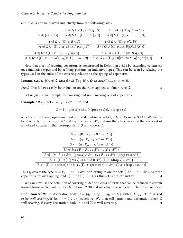
Chapter 3. Inductive-Coinductive Programming
and A ◁| Q can be derived inductively from the following rules.
A ◁| (∅; ·;A)A ◁| Q ∪ (Γ,x : 1;q;C)A ◁| Q ∪ (Γ;q[⟨ ⟩/x ];C)
A ◁| Q ∪ (Γ;q;B → C)A ◁| Q ∪ (Γ,x : B;q x ;C)
A ◁| Q ∪ (Γ;q;B ×C)A ◁| Q ∪ (Γ;q.pr1;B), (Γ;q.pr2;C)
A ◁| Q ∪ (Γ;q;νX . B)A ◁| Q ∪ (Γ;q.out;B[νX . B/X ])
A ◁| Q ∪ (Γ,x : B1 + B2;q;C)A ◁| Q ∪ (Γ,xi : Bi ;q[κi xi/x ];C) | i = 1, 2
A ◁| Q ∪ (Γ,x : µX . B;q;C)A ◁| Q ∪ (Γ,y : B[µX . B/X ];q[α y/x ];C)
Note that a set of covering copatterns is constructed in Definition 3.2.24 by extending copatternson coinductive types and by refining patterns on inductive types. This can be seen by relating thetypes used in the rules of the covering relation to the typing of copatterns:
Lemma 3.2.25. If A ◁| Q, then for all (Γ;q;B) ∈ Q we have Γ ⊢cop q : A⇒ B.
Proof. This follows easily by induction on the rules applied to obtain A ◁| Q.
Let us give some example for covering and non-covering sets of copatterns.
Example 3.2.26. Let U = Fµ → Bω → Bω and
Q = (· (pres x) s).hd, (· (pres x) s).tl, · (drop u) s,
which are the three copatterns used in the definition of selectµ : U in Example 3.2.11. We definetwo contexts Γ1 = x : F , s : Aω and Γ2 = u : Fµ , s : A
ω , and use these to check that there is a set ofannotated copatterns that corresponds to Q and covers U :
U ◁| (∅; ·; Fµ → Bω → Bω)U ◁| (y : Fµ ; · y;Aω → Aω)U ◁| (y : Fµ , s : A
ω ; · y s;Aω)U ◁| (z : F + Fµ , s : A
ω ; · (α z) s;Aω)U ◁| (x : F , s : Aω ; · (pres x) s;Aω), (u : Fµ , s : A
ω ; · (drop u) s;Aω)U ◁| (Γ1; (· (pres x) s).out;A ×Aω), (Γ2; · (drop u) s;Aω)
U ◁| (Γ1; (· (pres x) s).hd;A), (Γ1; (· (pres x) s).tl;Aω), (Γ2; · (drop u) s;Aω)
Thus Q covers the type U = Fµ → Bω → Bω . Non-examples are the sets ·.hd ; ·.tl ; ·.hd, as thesecopatterns are overlapping, and (· 0).hd ; (· 0).tl, as this set is not exhaustive.
We can now use the definition of covering to define a class of terms that can be reduced to certainnormal forms (called values, see Definition 3.2.30) and on which the reduction relation is confluent.
Definition 3.2.27. A declaration body D = q1 7→ t1; . . . ;qn 7→ tn with Γ;Σ ⊢bdy D : A is saidto be well-covering, if qi | i = 1, . . .n covers A. We then call terms t and declaration block Σwell-covering, if every declaration body in t and Σ is well-covering.
64

3.2. Programming with Equations
Example 3.2.28. By Example 3.2.26, we have that selectµ is well-covering.
Let us now put the covering relation to use. The class of terms that we have been advertising, onwhich the reduction relation is well-behaved, is given by the following definition.Definition 3.2.29. For a declaration block Σ and a type A, we define several sets of terms:
Λ=Σ(A) B t | ∅; Σ ⊢ t : A and t is well-coveringΛ=Σ B
∪A∈Ty
Λ=Σ(A)
Λ=(A) B Λ=∅ (A)
Λ= B Λ=∅
First, we show that every well-covering term is either a value or can be further reduced. Thenotion of value is given in the following definition.Definition 3.2.30. A term t of type A is a value if (i) A is an inductive type and t = c s for aconstructor c and a value s; (ii) A is coinductive; or (iii) t = x for some variable x .
Lemma 3.2.31 (Progress). Let A be a type and Σ a well-covering declaration block. For every termt ∈ Λ=
Σ(A), we have that either t is a value or that there is a t ′ with t −→Σ t ′.
Proof. The proof of this fact is easily adopted from [Abe+13, Sec. 5], where one crucially has toappeal to the two rules that distribute evaluation contexts and constructors over rlet-bindings.
On the same class of terms, we now also prove confluence. The details of the proof can be foundin Appendix A.Proposition 3.2.32. For any type A and any well-covering Σ, −→Σ is confluent on Λ=
Σ(A) and, inparticular, −→ is confluent on Λ=.
Let us briefly discuss what the relevance of the progress result and confluence is in the contextof this thesis. First of all, confluence allows us to simplify the definition of convertibility to t1 ≡t2 ⇐⇒ ∃t3. t1 t3 t2, see Section 2.1. More importantly, it ensures that constructors in headposition of terms are unique.Lemma 3.2.33. If t ∈ Λ=(A1 +A2) and t κi t
′ for some i ∈ 1, 2, then for all t ′′ with t κj t′′
we must have that i = j.
Proof. By confluence, there must be a term s with κi t′ s κj t
′′. Since reduction steps donot change or remove constructors, it follows that s = κi s
′ with i = j.
In combination with the progress lemma, we can find for every term of inductive type a weak headnormal form (WHNF) with unique constructors as follows. We denote the set family of all stronglynormalising terms by SN = SNAA∈Ty, whereby SNA = t ∈ Λ=(A) | t ↓, see Section 2.1.Lemma 3.2.34 (Weak Head Normal Forms). Let t ∈ SNA be a strongly normalising term. IfA = µX . B,then there is a t ′ ∈ SNB[µX . B/X ] with t ≡ α t ′. Otherwise, if A = B1 + B2, then there is i ∈ 1, 2 and at ′ ∈ SNBi with t ≡ κi t ′, and for every s with t ≡ κj s we have i = j.
Proof. Since t is strongly normalising, there is a normal form u with t u. The claim follows byapplying Lemma 3.2.31 to u. For sums, uniqueness of i is the content of Lemma 3.2.33.
65

Chapter 3. Inductive-Coinductive Programming
3.3. Relation Between λµν and λµν=Let us comment on the relation between the two presented calculi. As we have seen, they embodytwo different styles of recursion We can, however, emulate the recursion style of λµν in λµν=.Definition 3.3.1. We simultaneously define by induction on the type A the following three termconstructors in λµν=.
1. Given a type A and a term t with X ⊩ A : Ty and Γ;Σ ⊢ t : B → C , we define a termΓ;Σ ⊢ A[t ] : A[B]→ A[C];
2. given a term r with Γ;Σ ⊢ r : A[B/X ]→ B, we define an iterator Γ;Σ ⊢ Rµ r : µX .A→ B;
3. given a term r with Γ;Σ ⊢ r : B → A[B/X ], we define a coiterator Γ;Σ ⊢ Rν r : B → νX .A.The term A[t ] is given literally as in λµν (Definition 3.1.9), only with iter replaced by Rµ and coiterby Rν . For the iterator, we define
Rµ r B rlet f : µX .A→ B =· (α x) 7→ r (A[f ] x)
in f ,
and the coiterator, on the other hand, we define by
Rν r B rlet f : B → νX .A =(· x).out 7→ A[f ] (r x)
in f .
We then obtain for the terms in Definition 3.3.1 the same typing rules as in λµν .Lemma 3.3.2. The following typing rules hold in λµν= for the terms defined in Definition 3.3.1.
Γ;Σ ⊢ t : B → C
Γ;Σ ⊢ A[t ] : A[B/X ]→ A[C/X ]
Γ; Σ ⊢ r : A[B/X ]→ B
Γ;Σ ⊢ Rµ r s : µX .A→ B
Γ;Σ ⊢ r : B → A[B/X ]
Γ; Σ ⊢ Rν r s : B → νX .A
These terms are, moreover, well-covering if r , s and t are.
Proof. The proof for the first rule is again carried out by induction on A, just like in Lemma 3.1.10.That the typing rules of the iterator and coiterator hold is seen as follows. First, we show that thebodies for the coiteration and iteration are well-typed, where we use the typing rule for A[t ]. Forthe case of Rν , we let Dν =
(· x).out 7→ A[f ] (r x)
and Σ′ = Σ, (f : B → νX .A = Dν ). Then we
can derive that D is well-typed as follows.Γ;Σ′ ⊢ f : B → νX .A
Γ;Σ′ ⊢ A[f ] : A[B]→ A[νX .A]
Γ; Σ′ ⊢ r : B → A[B] Γ; Σ′ ⊢ x : B
Γ,x : B; Σ′ ⊢ r x : A[B]
Γ,x : B; Σ′ ⊢ A[f ] (r x) : A[νX .A]Γ; Σ′ ⊢bdy
(· x).out 7→ A[f ] (r x)
: B → νX .A
Similarly for the body of Rµ , we put Dµ =· (α x) 7→ r (A[f ] x)
and Σ′ = Σ, (f : B → νX .A = Dµ ),
allowing us to carry out the following derivation.Γ;Σ′ ⊢ f : µX .A→ B
Γ;Σ′ ⊢ A[f ] : A[µX .A]→ A[B] Γ,x : A[µX .A]; Σ′ ⊢ x : A[µX .A]
Γ,x : A[µX .A]; Σ′ ⊢ A[f ] x : A[B]
Γ,x : A[µX .A]; Σ′ ⊢ r (A[f ] x) : BΓ;Σ′ ⊢bdy
· (α x) 7→ r (A[f ] x)
: µX .A→ B
66

3.4. Conclusion and Related Work
Since the bodies are well-typed, it is clear that Rµ r and Rν r have the required types.Finally, well-covering follows also by a straightforward induction on the type A. We check, as
an example, that Rν r is well-covering. This requires us to construct an annotated set of copatternsthat corresponds to (· x).out, which can be constructed by the following derivation.
B → νX .A ◁| (∅; ·;B → νX .A)B → νX .A ◁| (x : B; · x ;νX .A)
B → νX .A ◁| (x : B; (· x).out;A[νX .A/X ])
Thus, (· x).out covers B → νX .A, as required, and Rν r is well-covering.
This definition allows us to translate terms of λµν to terms in λµν=.
Definition 3.3.3. We define a function (−) : Λ→ Λ= by induction on the terms of λµν :
⟨ ⟩ = ⟨ ⟩
κi t = κi t
α t = α t
πi t = t.priξ t = t.out
s t = s t
x = x
λx . t = λ· x 7→ t⟨s, t⟩ = λ
· .pr1 7→ t ; · .pr2 7→ s
iterµX .A (x . t) s = Rµ (λx . t) s
coiterνX .A t s = Rν (λx . t) s
κ1 x 7→ s ; κ2 y 7→ t u = λκ1 x 7→ s ; κ2 y 7→ t u
Theorem 3.3.4. Definition 3.3.3 gives rise to a map (−) : Λ→ Λ=, in the sense that terms of λµν aremapped to well-covering terms of λµν=. Moreover, it preserves types:
Γ ⊢ t : A =⇒ Γ ⊢ t : A.
Proof. Both well-covering and type preservation are proved by induction on terms. All cases, exceptthat for iter and coiter, are thereby immediate. That the translation of iter and coiter is well-coveringand type preserving has been proved in Lemma 3.3.2.
3.4. Conclusion and Related WorkThe purpose of this chapter was to give some understanding of how to program with inductive-coinductive data. We chose here two calculi that employ different ways of dealing with inductive andcoinductive data, and compared their corresponding strengths and weaknesses: The first calculusλµν is hard to use, but all terms are strongly normalising. On the other hand, λµν= is fairly easyto use, but we can write non-terminating programs in it. Note that we have not proved strongnormalisation of λµν in this chapter, this will be rectified in Chapter 7. We tackle the problem ofnon-termination in λµν= in the next chapter.
In Chapters 6 and 7, we will establish category theoretical and type theoretic extensions of thesimple calculus λµν to the setting of dependent types. This will allow us to intertwine programmingand reasoning. Also, we will give there further applications of inductive-coinductive programming.
67

Chapter 3. Inductive-Coinductive Programming
The calculi presented in this chapter have been discussed in one form or another in other places,so let us clarify the relation to existing work. Possibly the earliest calculi with mixed inductive-coinductive types were given by Mendler [Men87; Men91] and Hagino [Hag87]. Mendler combinesthereby the polymorphic λ-calculus with inductive and coinductive types, whereas Hagino bases hiscalculus on the notion of dialgebra, something we will come back to in Chapter 7. Hagino’s iterationand coiteration schemes match quite clearly with the ones we used in Section 3.1. Mendler [Men91],on the other hand, models the iteration principle using constants
RµX .A : ∀Y .(∀Z .(Z → Y )→ A→ Y )→ µX .A→ Y .
If we note that the type ∀Z .(Z → Y ) → A → Y corresponds with maps A[Y/X ] → Y , then wecan read the type of RµX .A as “for every type Y and every A-algebra there is a map µX .A → Y ”.Thus, also Mendler’s style of introducing iteration gives rise to the same iteration principle thatwe were using in λµν , cf. Section 3.3 and [UV96]. Similarly, also his coiteration principle matchesthat of λµν . Thus both calculi agree on the inductive and coinductive types, but Mendler’s calculusalso features (impredicative) polymorphism. This allows Mendler to obtain iteration and coiterationprinciples without having to introduce explicitly the action of types on terms, see [UV96; UV02] fora detailed discussion and [UV99a; Ven00] for a discussion from a category theoretical perspective.To ensure strong normalisation, Mendler, of course, allows fixed points only of positive types. Inthis respect, Mendler’s calculus [Men87; Men91] goes beyond λµν , as we only allow strictly positivetypes. In principle, we could also extend λµν and λµν= to arbitrary positive types, see [Mat99] foruseful examples, but this would make the later developments in this thesis much harder. Similarly,Greiner [Gre92] considered a language with positive inductive and coinductive types as well, butrestricts to top-level polymorphism. Finally, Howard [How92; How96a] proved confluence and strongnormalisation for a calculus that is essentially an extension of λµν to positive types, and implementedthis calculus in the Lemon language [How95]. Interestingly, Howard [How96a] extends his calculusalso with an operation force : νX .A → µX .A for, what he calls, pointed types. This operationintroduces full recursion into the calculus for pointed types, essentially by turning the categoryassociated to the calculus into an algebraically compact category à la Freyd [Fre90].
Besides calculi with mixed inductive-coinductive types, one can find in the literature many calculiwith just inductive types [BDS13; Con97; Gim95; Mat99; Wer94], only coinductive types [Møg14]and calculi with one-layer inductive or coinductive types [Geu92]. Of these, most are based oniteration/coiteration schemes to avoid termination issues. Since programming with equational defin-itions is much more practical, as we have seen in Section 3.2, also calculi that support programmingwith recursive equations have been proposed. The calculus in Section 3.2 is, as mentioned, basedon the work by Abel et al. [Abe+13]. The termination issue for such calculi is being dealt with by,for example, Abel and Pientka [AP13], Atkey and McBride [AM13], Barthe et al. [Bar+04], Coquand[Coq93], Giménez [Gim95], Sacchini [Sac13] and Xi [Xi01].
Finally, syntactic specification formats for elements of final coalgebras have been proposed inseveral forms. The formats that are closest to the specifications that can be given in λµν= arethe behavioural differential equations (BDE) described, for example, by Hansen et al. [HKR17],Kupke and Rutten [KR08] and Rutten [Rut03]. To guarantee (unique) solutions to BDEs, Kupke andRutten [KR08] define a notion of complete sets of equations. These correspond to covering sets ofcopatterns, which we used to ensure that normalising terms have weak head normal forms withunique constructors in head position (Lemma 3.2.34). An important difference between the systems
68

3.4. Conclusion and Related Work
of equations developed in [KR08] and copattern equations is that specifications in λµν= can onlybe given on fixed point types, which correspond to final coalgebras. In contrast, the equationsin [KR08] can be given on so-called observational coalgebras, which are coalgebras for which themap into the final coalgebra is injective. It would be interesting to study a type theory that allowsthe specification of sub-types of largest fixed point types by specifying additional properties thatelements of that type must satisfy, see [Bas15b] for an example. Another approach to specificationsthat do not force the use of iteration and coiteration schemes are cyclic proof systems and games.These have, for example, been investigated by Cockett [Coc01] and Santocanale [San02a; San02b].
Notes10 Note that the the addition of natural numbers can also be defined without iteration on functions by
usingд+ B λm. κ1 y 7→m ; κ2 k 7→ suc k x
plus B λnm. iterNat (x .д+m) n
instead. However, it is illustrative to see how the function space can be exploited in iteration. Ancommon example of a function that can only be defined with higher-order iteration is the Ackermannfunction.
11 The extra case for types that do not use any variables in the definition of the action of types onterms is needed in a very subtle way. Not only does this give us better computation rules, but it isactually crucial in the proof of Proposition 4.1.9. An elegant way around this extra case would be touse externally given monotonicity witnesses, as in [Mat99; UV02]. We will discuss other approachesin the conclusion of this chapter.
12 It should be noted that programming just with iteration and coiteration schemes can be very chal-lenging. For example, the predecessor on natural numbers or the construction of a stream from itshead and tail are surprisingly difficult to define. In the setting of initial algebras and final coalgebrastheir definitions follow from Lambek’s lemma (Lemma 2.5.4), but in a syntactic calculus it takes abit of ingenuity to come up with their definitions. For the predecessor function this even lead to anice story about Kleene having an epiphany at the dentist of how to implement the predecessor inpure λ-calculus [Cro75]. This problem can be remedied by generalising the concept of iteration andcoiteration that we used here, to that of primitive recursion and primitive corecursion, respectively,see [BDS13; Geu92; Lei89; UV99c; Ven00; VU98]. We will not discuss this further though, as it notrelevant to us here, and since these problems do not occur in the calculus introduced in Section 3.2below. Also the dependent type theory in Chapter 7 immediately admits primitive recursion.
13 One could continue to prove relevant properties about this calculus like subject reduction (types ofterms are preserved under reduction steps), confluence (any two reduction sequences originating atthe same term can be joined), progress (every term can be reduced to a value, where a value is aterm that has been constructed only by introduction rules, projection and weakening) and strongnormalisation (no term has an infinite reduction sequence). However, we refrain from doing so, as(variations of) the calculus λµν have been extensively studied. Proofs of strong normalisation can,for example, be found in [AA99; How92; Mat99], whereby confluence is also proven by Howard
69
Chapter 3. Inductive-Coinductive Programming
[How92]. We just note here that λµν can be encoded into other calculi presented in this thesis,while preserving reduction steps. More specifically, λµν is a (strongly normalising) fragment ofthe calculus considered in Section 3.2, from which we can obtain subject reduction, progress andconfluence, see Section 3.3. λµν is also a non-dependent fragment of the dependent type theorystudied in Chapter 7, from which we can obtain strong normalisation. Hence, we will not study theproperties of the present calculus in isolation.
14 We do not have a precise notion of predicate at this point, but we just assume an intuitive under-standing that we can check whether a predicate holds for a given element of A.
15 We note that one can also define by iteration a function _@_ : Aω → Nat → A that, given astream s and an index n : Nat, returns the element s @ n at position n in s . Moreover, thereis a stream nats : Natω that enumerates the natural numbers. It is then fairly easy to see that(select x s)@ n ≡ s @ (select x nats @ n) for every n ∈ N. From these considerations, it follows thatmod x n ≡ select x nats@n, which gives us a more direct way to express mod and a direct link withselect. To ease calculations, we stick here to the explicit definition of mod though.
70

CHAPTER 4
Observations
In this sense, meanings control us, inculcate obedience to the discipline inscribed in them. And this is byno means purely institutional or confined to the educational process. […] The right word in a new situationdoes not always readily present itself. Language sometimes seems to lead a life of its own. Words are unruly“They’ve a temper, some of them”, Humpty Dumpty goes on to observe.
— Catherine Belsey, “Poststructuralism”, 2002.
In the last chapter, we defined the two calculi λµν and λµν=. The aim of this chapter is to makesome first steps towards reasoning principles for the programs of these calculi.
One of the most important ingredients in reasoning about programs is the ability to comparetheir behaviour. So far, we are only able to compare programs on the basis of their computationalbehaviour , which is given by the reduction relations on the terms of the two calculi. In particular,these reduction relations give rise to convertibility as their equivalence closure. Convertibility canreadily be used to compare the computational behaviour of programs. However, this comparison isoften too fine-grained to be useful. For instance, the terms 1ω and odd alt are not convertible toeach other. But we have
1ω .hd ≡ 1 1ω .tl ≡ 1ω (Example 3.2.16)odd alt .hd ≡ 1 odd alt .tl ≡ odd alt, (Example 3.2.19)
from which we would like to infer that the programs 1ω and odd alt produce the same streamentries but arrive at them through different computations. The question is now how we can formallycharacterise that they have “the same entries”?
An important notion that pervades reasoning about programs is that of observations, which determ-ine in turn the observational behaviour of programs. For example, on streams the two fundamentalobservations are taking the head and the tail of a stream. Functions, on the other hand, haveas many observations as they have possible arguments, since we can observe the outcome of theapplication of a function to any argument. In a mixed inductive-coinductive setting, general ob-servations on programs are more complex. For instance, what is the observational behaviour ofthe term 1, or of the selector oddF from Example 3.2.11? In the former case, 1 is as a value, seeDefinition 3.2.30, completely determined by its computational behaviour. However, for oddF wehave oddF.out ≡ drop (pres oddF), thus we should clearly consider the constructors drop and presas part of the observational behaviour of oddF. This raises the question of how to characterisethe observational behaviour for general inductive-coinductive programs. We will resolve this inSection 4.1.2 by introducing a type-driven notion of observation in the form of a modal logic ofprogram tests, which will formally define what the observable behaviour of program is. Havingdefined the observational behaviour of programs, we can also say that programs are observationallyequivalent, given that they show the same observational behaviour.
Despite the fact that comparing the observational behaviour of programs is often more useful, alsocomputational behaviour plays a role. For example, the coiteration on streams over A (Section 3.3)
71

Chapter 4. Observations
has the property that(Rν r s).hd ≡ (r s).pr1,
where r : B → A × B and s : B. Since conversions that arise from iteration and coiteration can bevery complex and tedious to carry out by hand, it lifts a great burden from us if we can pass theseto a machine. This, however, requires that the conversion relation is computable, which would fail ifwe had, for example, that Rν ≡ h for all homomorphisms h : B → Aω that fulfil h.hd ≡ (r s).pr1 andh.tl ≡ h ((r s).pr2). Rather, we will say that Rν r and all such homomorphisms h are observationallyequivalent, which we write as Rν r ≡obs h.
Our goal in Section 4.2 is to analyse and compare both computational and observational behaviourin a common framework, towards which we proceed in two steps. The first step in understandingthe difference between the two behaviours is the use of categories in which objects are typesand morphisms are equivalence classes of terms up-to convertibility. Thus, we first take only thecomputational behaviour into account. In this setup, we can already identify some concepts thatresemble category theoretical constructions. For instance, we will find that product types are weakproducts, in other words, they have projections and maps can be paired, but this pairing is notunique. Next, we will extend these categories to 2-categories, where the objects and morphisms areas before but 2-cells relate observationally equivalent terms. Setting up 2-categories in this way hastwo effects. First of all, we can identify more precisely the structure that the types come with. Forexample, we have that the product types give rise to pseudo-products, which in this case meansthat the pairing is unique up-to observational equivalence. Secondly, we are able to distinguishthe computational from the observational behaviour, in the sense that computational equivalence isgiven as equality of morphisms, while observational equivalence is situated at the level of 2-cells.This has the effect that, for instance, the identity (Rν r s).hd = (r s).pr1 holds in the 2-category, butin general we only have an isomorphism Rν r h, see Definition 2.6.3, between the coiteration anda homomorphism h. Thus, this 2-category theoretical setup allows to identify the properties anddifferences of computational and observable behaviour of programs in λµν and λµν=.
The purpose of this chapter is to develop the fundamental ability to compare the behaviour ofprograms, specifically programs of inductive-coinductive types. Towards the end of Section 4.1, weare thus able to express interesting properties of programs in λµν and λµν=. In Chapter 5, wewill then provide techniques to prove such properties. Also the category theoretical description ofthe types and terms will reappear in Chapter 6, although there we will deal with dependent types.Finally, in Chapter 7, we will be able to compare programs in the there provided dependent typetheory, without having to resort to an external logic or set theory.
Original Publication Section 4.1 has been presented in [BH16]. In the same paper, a categorytheoretical account of the calculus from Section 3.2 has also been given. However, the analysis wegave there was not very precise, as we did not make any distinction between computations andobservations. This is remedied in Section 4.2.
4.1. Observational Equivalence and NormalisationWe have already come across the notion of observational behaviour of programs a couple of times.The purpose of this section is to make this notion precise. In what follows, we introduce test formulas
72

4.1. Observational Equivalence and Normalisation
that allow us to carry out observations on terms of λµν and λµν=. We then use these test formulasto define observational equivalence, which compares terms on the basis of their observational ratherthan their computational behaviour. Moreover, we use test formulas to single out the observationallynormalising terms of λµν=, which are those terms that respond to any observation with a stronglynormalising term.
Test formulas are formulas of a multi-modal logic, where the modalities capture the observationsthat can be carried out on terms of a given type. Thus, test formulas are themselves typed. Theseformulas are closely related to the testing logic considered in [San11, Sec. 6.2], and the many-sortedcoalgebraic modal logics for polynomial functors studied, for example, by Jacobs [Jac01] and Kupke[Kup06, Sec. 2.1.2]. Considering how the calculi in Chapter 3 were set up, the reader might haveguessed by now that the essential observations on terms of product- and ν-type are given by thecorresponding destructors π1, π2 and ξ , respectively. What needs clarification are observations onterms of inductive type and on functions.
The distinguishing feature of inductive types are the constructors. This is reflected both in thecase distinction for sums and the recursion principle in λµν , and the covering of patterns in λµν=.In both calculi, we construct programs on sum and µ-types from programs that cover all possibleconstructor cases. These considerations lead us to use modalities in the testing logic that inspectthe constructor in the head position of terms, see Definition 4.1.19.
For tests on terms of function type we would expect that an observation amounts to functionapplication, thus there should be a modality for each possible argument. However, there is a caveat.If we allow any argument, then we could inspect the computational behaviour of terms, which shouldnot be an observable property. Hence, it should also not be taken into account for observationalequivalence. Consider, for example, the following two terms f1, f2 : Nat→ Nat in λµν=.
f1 B λ· 0 7→ 0 ; · (suc n) 7→ 1
f2 B λ
· 0 7→ 0 ; · (suc 0) 7→ 1 ; · (suc (suc n)) 7→ 1
Then for the non-terminating program Ω from Example 3.2.21, we have f1 (suc Ω) −→ 1, whereasf2 (sucΩ) does not have a weak head normal form. Thus, we can distinguish f1 and f2 by applyingthem to a term that does not have a normal form. If we restrict attention to strongly normalisingterms t though, then f1 t ≡ f2 t . For this reason, the modalities on function types will range onlyover the observationally normalising terms of λµν=, see Definition 4.1.3.
Observationally normalising terms subsume both terminating computations of inductive typeand, what is usually called, productive programs of coinductive type. In the case of streams, therequirement that a term t : Natω is observationally normalising will be defined as follows. First, thehead of t is a strongly normalising term of type Nat, that is, t .hd ≡ n for some n ∈ N. Second, its tailt .tl is strongly normalising and again observationally normalising. What this gives us, is that we areable to interpret t as a function t† : N → N in the set-theoretic sense by iteratively extracting theentries of t , in other words we put t†(0) = n and t†(k + 1) = (t .tl)†(k). In general, the restrictionto observationally normalising terms allows us to interpret these as set-theoretic (total) functions.
4.1.1. Observational NormalisationAs we discussed in the introduction, we want to test terms of function type only on terms thatnormalise under any observation. Thus, to be able to define tests for λµν=, our first task is to define
73

Chapter 4. Observations
the corresponding class of, what we call here, observationally normalising terms. The intention isto capture the largest class of terms that can serve as an interpretation for types, which separatesinductive and coinductive types. In particular, this means that all terms in that class must be stronglynormalising, that is, correspond to terminating computations, and the class must be closed underobservations. For instance, given observationally normalising terms t and s with t : A → B ands : A, also the application t a should be observationally normalising. Since we are interested in thelargest class of terms, the iterators and coiterators, which we introduced in Definition 3.3.1, shouldalso be in that class. The definition of observational normalisation and the proof that the iteratorsand coiterators are observationally normalising are our concern in the remainder of the presentsubsection. Closure under observations in proved in Theorem 4.1.17 in the next subsection.
Before we come to the definition of observational normalisation, we need to introduce somenotation. First of all, to define observational normalisation on open terms, we need to generalisethe notion of substitution that we used before, see Definition 3.2.12. Recall that a substitution is amap σ that assigns to variables in TeVar terms in λµν or λµν=. Moreover, we denoted the type ofx in a context Γ by Γ(x).
Definition 4.1.1. Let U = UAA∈Ty be a family of sets indexed by types. For a context Γ, wesay that a substitution σ is U -Γ-closing, if dom(Γ) ⊆ dom(σ) and for every x ∈ dom(Γ) we haveσ(x) ∈ UΓ(x). We denote by Subst(U ; Γ) the set of all U -Γ-closing substitutions.
Secondly, we will define observationally normalising terms on open types, whose variables willbe interpreted as sets of terms. This leads us to the following definition.
Definition 4.1.2. Let Θ be a type variable context and υ a substitution of closed types for thevariables in Θ, see Definition 3.1.1. We denote by IΘ,υ be set of valuation functions V that mapvariables X in Θ to subsets of Λ=
υ(X ), that is,
IΘ,υ =V : Θ→ P(Λ=)
V (X ) ⊆ Λ=υ(X )
.
Moreover, let us denote by ε the empty valuation. Finally, if V ∈ IΘ,υ , A ∈ Ty and U ⊆ Λ=A , then we
write V [X 7→ U ] for the updated valuation in I(Θ,X ),υ[A/X ].
Now we are in the position to define the set of observationally normalising terms. We do thisin three steps: First, we define by iteration on types an operator WD (“well-defined”) that takesan open type and a valuation for the variables of that type as input. This first step is required todefine observationally normalising terms on fixed point types. Next, the set ON of observationallynormalising terms is given by evaluating WD on closed types. Finally, observational normalisationon open terms is defined in terms ON and ON-closing substitutions. These three steps are capturedin the following definitions.
Definition 4.1.3. Let Θ be a type variable context, υ ∈ TySubst(Θ), and V ∈ IΘ,υ . Given a type A
74

4.1. Observational Equivalence and Normalisation
with Θ ⊩ A : Ty, we define WDυ,VA ⊆ Λ=
A[υ] by iteration on A as follows.WDυ,V
1 = SN1
WDυ,VX = V (X )
WDυ,VA1+A2
=∪i=1,2
s ∈ SN(A1+A2)[υ]
(∃s ′. s κi s′) ∧
(∀s ′. (s κi s
′) =⇒ s ′ ∈WDυ,VAi
)WDυ,V
A1×A2=
s ∈ SN(A1×A2)[υ]
∧i=1,2
s .pri ∈WDυ,VAi
WDυ,V
A→B =s ∈ SNA→B[υ]
∀t ∈WD(),εA . s t ∈WDυ,V
B
WDυ,V
µX .A = µU .s ∈ SN(µX .A)[υ]
(∃s ′. s α s ′)
∧(∀s ′. (s α s ′) =⇒ s ′ ∈WDυ[µX .A/X ],V [X 7→U ]
A
)WDυ,V
νX .A = νU .s ∈ SN(νX .A)[υ]
s .out ∈WDυ[νX .A/X ],V [X 7→U ]
A
,
In this definitions, the fixed points are taken in the complete lattice of subsets of Λ=, which existbecause WDυ,V
A is clearly monotone in V in each case. For a closed type A, that is, if Θ is empty,we define the set family ONA of observationally normalising terms of type A by16
ONA BWD(),εA .
Moreover, given a context Γ, we define ONΓA to be the set of all terms t such that t ∈ SN and
t [σ ] ∈ ONA for any ON-Γ-closing substitution σ , see Definition 4.1.1. Finally, given a type A withΘ,X ⊩ A : Ty, we define a monotone function
Ψυ,VA : P
(Λ=A[µX .A/X ][υ]
)→ P
(Λ=A[µX .A/X ][υ]
)Ψυ,VA (U ) =
s (∃s ′. s α s ′) ∧
(∀s ′. (s α s ′) =⇒ s ′ ∈WDυ[µX .A/X ],V [X 7→U ]
A
)∩ SN,
so that WDυ,VµX .A = µU .Ψυ,V
A (U ).
Before we continue, let us remark on the use of the least fixed point the definition of WD inthe case of µ-types. This least fixed point ensures that a term can only be finitely often unfolded,which is crucial in ensuring that the iterator that we introduced in Definition 3.3.1 is observationallynormalising. This, in turn, will allow us to prove in Section 4.2 that in the category of observation-ally normalising terms, all µ-types are initial algebras. Interestingly, in the calculus λµν= strongnormalisation and admitting only finitely many unfolding steps do not coincide, as the followingexample shows.17
Example 4.1.4. Given a closed type A, we can define the type A∗ of lists over A to be µX . 1+A×X .Suppose that we are given a term a of type A, then the following is a program in λµν=.
p : A ×A∗
p.pr1 = a
p.pr2 = α (κ1 p)
75

Chapter 4. Observations
Note that p.pr2 denotes an infinite list of a’s, but p.pr2 ∈ SNA∗ . However, one can show p.pr2 < ONA∗
by induction on a hypothetical proof of p.pr2 ∈ ONA∗ .
As intended, strong normalisation is implied by observational normalisation.
Lemma 4.1.5. There is an inclusion ON ⊑ SN of set families, that is, ONA ⊆ SNA for all A ∈ Ty.
Proof. To prove that ON ⊑ SN holds, one shows for all types A with Θ ⊩ A : Ty, substitutionsυ ∈ TySubst(Θ) and valuations V ∈ IΘ,υ with V (X ) ⊆ SNυ(X ) that WDυ,V
A ⊆ SNA[υ] by inductionon A. This induction is then almost trivial, except for the cases of µ- and ν-types, in which we haveto use the fixed point properties. The result follows for closed types by definition of ON.
In following example we illustrate that the definition of observational normalisation includes termsthat do not necessarily correspond to guarded recursive equations [Bar04] or guarded recursiveschemes [Gim95]. This example is intended for readers who are familiar with stream differentialequations (SDE) [HKR17] with the goal being an interpretation of some SDEs in λµν=.
Example 4.1.6. To simplify the development in this example, we restrict attention to SDEs over asignature with two symbols, say f1 and f2, each of arity 2. Given a type A, let us denote the productA ×A by A2. We can represent a signature with two symbols of arity 2 by the type
F B X 2 + X 2,
in the sense that the type F ∗ of terms over this signature with variables in Y is given by
F ∗ B µX . F + Y
with Y ⊩ F ∗ : Ty. Let us now fix a type V of four elements that we will use as stream variables:
V B (1+ 1) + (1+ 1).
We denote these variables by
x B κ1 (κ1 ⟨ ⟩) y B κ1 (κ2 ⟨ ⟩)
x′ B κ2 (κ1 ⟨ ⟩) y′ B κ2 (κ2 ⟨ ⟩).
The variables represent two streams x and y, and their tails x′ and y′ in the syntax of SDEs.Let A ∈ Ty. A system of SDEs over F is given by four observationally normalising terms
hi : A2 → A, i = 1, 2
di : A2 → F ∗[V ], i = 1, 2,
We interpret these terms as the following system of stream differential equations, see [HKR17].
fi (s, t).hd = hi (s .hd, t .hd)fi (s, t).tl = di (s .hd, t .hd)[s/x, t/y, (s .tl)/x′, (t .tl)/y′]
(4.1)
These equations say that the head and tail of fi (s, t) are given by evaluating at the head of s andt the maps hi and di , respectively. In the case of the tail, we also need to substitute the input
76

4.1. Observational Equivalence and Normalisation
streams s and t and their tails into the expression that results from di . The goal of this example isto implement the substitution and the above system of SDEs in λµν=.
We first deal with substitution. Let I B V → Aω , which is the type of interpretations of thevariables inV over streams. The substitution operation we need is a map that, given an interpretationu : I , replaces every variable v : V in a term in F ∗[V ] by u v , thus obtaining a term in F ∗[Aω ]. This isin fact just given by F ∗[u] : F ∗[V ]→ F ∗[Aω ], see Definition 3.3.1. To simplify notation, we introducea term mkI : Aω ×Aω → I that allows us to construct the substitution in (4.1):
mkI u x = u .pr1 mkI u y = u .pr2mkI u x′ = u .pr1.tl mkI u y′ = u .pr2.tl
The substitution in (4.1) is then given for stream terms s and t by mkI ⟨s, t⟩. We can now interpret(4.1) in λµν= by mutual recursion:
⌊−⌋ : F [Aω ]→ Aω
⌊κi u⌋ .hd = hi ((hd × hd) u) i = 1, 2
⌊κi u⌋ .tl =⌊F ∗[mkI u] (di ((hd × hd) u))
⌋µ i = 1, 2
⌊−⌋µ : F ∗[Aω ]→ Aω
⌊α (κ1 t)⌋µ = ⌊F [⌊−⌋µ ] t⌋⌊α (κ2 s)⌋µ = s
The way ⌊−⌋ corresponds to (4.1) is as follows. First of all, recall that the SDE term “fi (s, t)” isgiven by the term κi ⟨s, t⟩ of type F [Aω ]. Thus, the cases for head and tail in the definition of⌊κi u⌋ correspond to the head and tail cases in (4.1). This also readily explains the definition of thehead of ⌊−⌋. However, the tail case needs a few more words of explanation. In (4.1), a substitutionand the complex SDE term di are used. The substitution is carried out in the definition of ⌊−⌋ byapplying F ∗[mkI u] to di . Afterwards, we use ⌊−⌋µ to give an interpretation of the SDE term, inwhich variables have been replaced by elements of A and streams over A. Interpreting such a termproceeds then by iteration, where each function symbol, denoted by t in the definition of ⌊−⌋µ , isagain interpreted by appealing to ⌊−⌋, and each stream variable is interpreted by its assigned stream.
Note that in the tail-case of ⌊−⌋ the outermost function is not ⌊−⌋ itself. Thus, the above definitionis not syntactically guarded and it is thus not immediately clear that it is well-defined. We claim,however, that ⌊−⌋ ∈ ON. Since we first need that the action F ∗[−] on terms preserves observationalnormalisation, we defer the proof.
It should also be noted that ⌊−⌋ can be implemented in Agda by using sized types. Sized typesallow the check for well-definedness of recursive equations through the use of a typing mechanism,see for example [AP13]. We will not discuss this here further, but see [Bas16] for an implementationof ⌊−⌋ over a general signature that uses sized types in Agda.
Throughout the remainder of this section we show that the iterator and coiterator from Defini-tion 3.3.1 are observationally normalising. This is what one would expect, as the encoding of thecalculus λµν into λµν= from Section 3.3 should restrict to ON because all the terms in λµν arestrongly normalising. However, the proof is fairly involved, since the iterator and coiterator aredefined simultaneously with the action of open types on terms. This forces us to prove also observa-tional normalisation the iterators, coiterators and type actions simultaneously, see Proposition 4.1.9below.
77
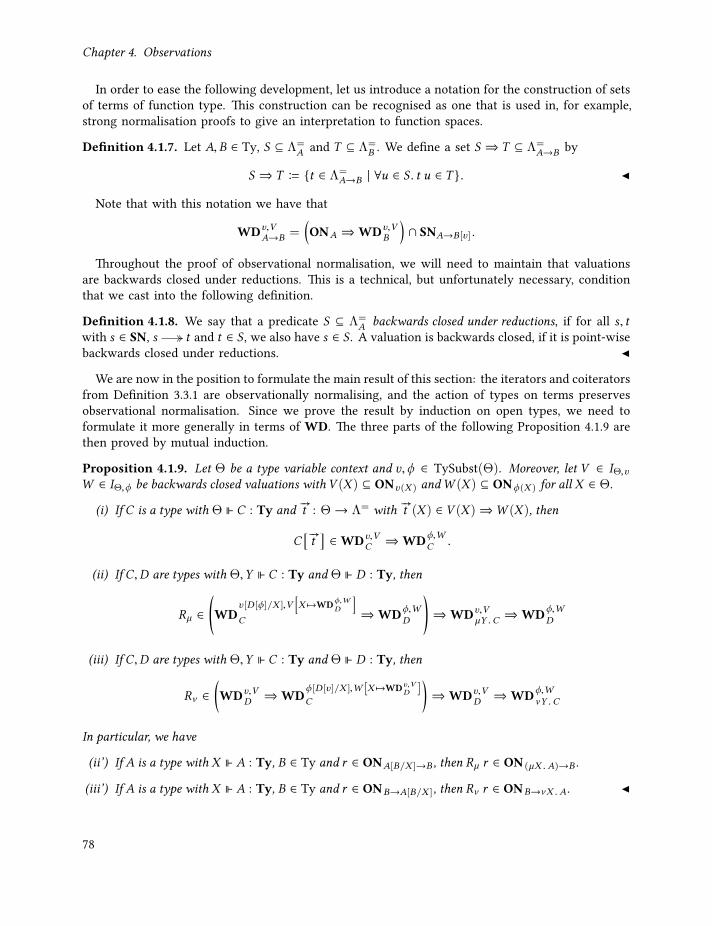
Chapter 4. Observations
In order to ease the following development, let us introduce a notation for the construction of setsof terms of function type. This construction can be recognised as one that is used in, for example,strong normalisation proofs to give an interpretation to function spaces.
Definition 4.1.7. Let A,B ∈ Ty, S ⊆ Λ=A and T ⊆ Λ=
B . We define a set S ⇒ T ⊆ Λ=A→B by
S ⇒ T B t ∈ Λ=A→B | ∀u ∈ S . t u ∈ T .
Note that with this notation we have that
WDυ,VA→B =
(ONA ⇒WDυ,V
B
)∩ SNA→B[υ].
Throughout the proof of observational normalisation, we will need to maintain that valuationsare backwards closed under reductions. This is a technical, but unfortunately necessary, conditionthat we cast into the following definition.
Definition 4.1.8. We say that a predicate S ⊆ Λ=A backwards closed under reductions, if for all s, t
with s ∈ SN, s t and t ∈ S , we also have s ∈ S . A valuation is backwards closed, if it is point-wisebackwards closed under reductions.
We are now in the position to formulate the main result of this section: the iterators and coiteratorsfrom Definition 3.3.1 are observationally normalising, and the action of types on terms preservesobservational normalisation. Since we prove the result by induction on open types, we need toformulate it more generally in terms of WD. The three parts of the following Proposition 4.1.9 arethen proved by mutual induction.
Proposition 4.1.9. Let Θ be a type variable context and υ,φ ∈ TySubst(Θ). Moreover, let V ∈ IΘ,υW ∈ IΘ,φ be backwards closed valuations with V (X ) ⊆ ONυ(X ) andW (X ) ⊆ ONφ(X ) for all X ∈ Θ.
(i) If C is a type with Θ ⊩ C : Ty and #—t : Θ→ Λ= with #—
t (X ) ∈ V (X )⇒W (X ), then
C[
#—t]∈WDυ,V
C ⇒WDφ,WC .
(ii) If C,D are types with Θ,Y ⊩ C : Ty and Θ ⊩ D : Ty, then
Rµ ∈(WD
υ[D[φ]/X ],V[X 7→WDφ,W
D
]C ⇒WDφ,W
D
)⇒WDυ,V
µY .C ⇒WDφ,WD
(iii) If C,D are types with Θ,Y ⊩ C : Ty and Θ ⊩ D : Ty, then
Rν ∈(WDυ,V
D ⇒WDφ[D[υ]/X ],W [X 7→WDυ,VD ]C
)⇒WDυ,V
D ⇒WDφ,WνY .C
In particular, we have
(ii’) If A is a type with X ⊩ A : Ty, B ∈ Ty and r ∈ ONA[B/X ]→B , then Rµ r ∈ ON(µX .A)→B .
(iii’) If A is a type with X ⊩ A : Ty, B ∈ Ty and r ∈ ONB→A[B/X ], then Rν r ∈ ONB→νX .A.
78

4.1. Observational Equivalence and Normalisation
In what follows, we prepare the proof of Proposition 4.1.9. First of all, we prove that WD isbackwards closed. This will be necessary, since we will interpret variables at fixed point types byappealing to to WD.
Lemma 4.1.10. Suppose A is a type with Θ ⊩ A : Ty, υ a substitution and V ∈ IΘ,υ a backwards closedvaluation. Then also WDυ,V
A is backwards closed. In particular, for all B ∈ Ty, t ∈ ONB and s ∈ SN withs t , we have s ∈ ONB .
Proof. Let A, υ and V be as assumed in the lemma. We show that WDυ,VA is backwards closed by
induction on A.
• Note that WDυ,V1 is backwards closed by definition, and that WDυ,V
X is backwards closed bythe assumption that V is backwards closed.
• In case of the sum types, suppose that t ∈ WDυ,VA1+A2
and that s t . To prove thats ∈WDυ,V
A1+A2, we have to provide an i ∈ 1, 2, such that there is an s ′ with s κi s
′ andsuch that for any such s ′, we have s ′ ∈ WDυ,V
Ai. Since t κi t
′ for some i ∈ 1, 2 and t ′,we also have a weak head reduction s κi t . Thus, we can use s ′ = t ′. Suppose now thats κi s
′ for some s ′. Then, by confluence, there is a t ′ with t κi t′ κi s
′. Hence,we also have s ′ t ′. Since t ∈WDυ,V
A1+A2, we obtain t ′ ∈ t ∈WDυ,V
Aiand, by the induction
hypothesis, that s ′ ∈WDυ,VAi
. Putting everything together, we have s ∈WDυ,VA1+A2
.
• Similarly, the case of µ-types is proven by defining
S Bt ∈WDυ,V
µX .A
∀s . (s t) =⇒ s ∈WDυ,VµX .A
and then showing that WDυ,V
µX .A ⊆ S by appealing to the definition of WDυ,VµX .A as a least
fixed point, confluence and the induction hypothesis.
• For function types, we have to show for given t ∈ WDυ,VA→B and s t , that s ∈ SN and
that for all u ∈ ONA that s u ∈ WDυ,VB . The former is given by assumption, while the latter
follows from the induction hypothesis from the fact that t u ∈ WDυ,VB and because s t
induces s u t u.
• The case of products follows by a similar argument as in the case of function types.
• To prove the case of ν-types, one easily shows, by using the induction hypothesis and thefact that WDυ,V
νX .A defined as a largest fixed point, that the set S given by
S B s ∈ SNνX .A[υ] | s t
is contained in WDυ,VνX .A. The claim of the lemma then immediately follows.
Next, we show that that WD is closed under identity maps, composition and the formation ofpattern matching and pairs. These results give us directly the proof of Proposition 4.1.9.(i) in thecase of function, sum and product types.
79

Chapter 4. Observations
Lemma 4.1.11. Let A,A1,A2 be types with Θ1 ⊩ A,A1,A2 : Ty, B,B1,B2 with Θ2 ⊩ B,B1,B2 : Ty, Ca type with Θ3 ⊩ C : Ty, υ, φ and ω substitutions for, respectively, Θ1, Θ2 and Θ3,V ∈ IΘ1,υ ,W ∈ IΘ2,υ ,andU ∈ IΘ3,ω . Then the following holds.
(i) id ∈WDυ,VA ⇒WDυ,V
A
(ii) If s ∈WDυ,VA ⇒WDφ,W
B and t ∈WDυ,VB ⇒WDφ,U
C , then t s ∈WDυ,VA ⇒WDω,U
C .
(iii) If ti ∈WDυ,VAi⇒WDφ,W
B for all i ∈ 1, 2 then
λκ1 x 7→ t1 x ; κ2 y 7→ t2 y ∈WDυ,VA1+A2
⇒WDφ,WB .
(iv) If ti ∈WDυ,VA ⇒WDφ,W
Bifor all i ∈ 1, 2 then
λx . ⟨t1 x , t2 x⟩ ∈WDυ,VA ⇒WDφ,W
B1×B2.
(v) If ti ∈ WDυ,VAi⇒ WDφ,W
Bifor all i ∈ 1, 2 then t1 + t2 ∈ WDυ,V
A1+A2⇒ WDφ,W
B1+B2and
t1 × t2 ∈WDυ,VA1×A2
⇒WDφ,WB1×B2
.
Proof. (i) SinceWDυ,VA is backwards closed by Lemma 4.1.10, id ∈WDυ,V
A ⇒WDυ,VA immediately
follows from id u u for u ∈WDυ,VA .
(ii) Again by using Lemma 4.1.10, closure of WD under composition follows directly from thedefinition of WD and ⇒.
(iii) Closure under pattern matching is given as follows. To show λκ1 x 7→ t1 x ; κ2 y 7→ t2 y ∈WDυ,V
A1+A2⇒WDφ,W
B , suppose s ∈WDυ,VA1+A2
. Then there is an i ∈ 1, 2 and an s ′ ∈WDυ,VAi
,such that s κi s
′. This gives us λκ1 x 7→ t1 x ; κ2 y 7→ t2 y s ti s′ and, by assumption,
that ti s ′ ∈ WDφ,VB . Hence, by Lemma 4.1.10, λκ1 x 7→ t1 x ; κ2 y 7→ t2 y s ∈ WDφ,V
B , andthus λκ1 x 7→ t1 x ; κ2 y 7→ t2 y ∈WDυ,V
A1+A2⇒WDφ,W
B .
(iv) The case for pairing is analogous to that for pattern matching.
(v) This follows immediately from closure under composition, and from closure under patternmatching and pairing, respectively.
After all this preliminary setup, we can finally proceed to prove the main result of this section.
Proof of Proposition 4.1.9. We prove the three parts of the proposition mutually by induction on C .
(i) Let C be a type with Θ ⊩ C : Ty and #—t with #—
t (X ) ∈ V (X ) ⇒W (X ), as in the proposition.To prove C
[#—t]∈WDυ,V
C ⇒WDφ,WC , we proceed by distinguishing the cases for C .
• If C is closed or C = 1, then C[
#—t]
= idC . The proof is then immediate fromLemma 4.1.11.(i).
80

4.1. Observational Equivalence and Normalisation
• For variables, we have X [#—t ] =
#—t (X ). By assumption, we have #—
t (X ) ∈ V (X )⇒W (X )
and thus #—t (X ) ∈WDυ,V
X ⇒WDφ,WX .
• The cases for sum, product and function types are given immediately by Lemma 4.1.11and the induction hypothesis.
• For the case of least fixed point types, recall that
(µY .C)[
#—t]= Rµ
(α C
[#—t , id
] ),
which means we have to prove that
Rµ(α C
[#—t , id
] )∈
(WDυ,V
µY .C ⇒WDφ,WµY .C
). (4.2)
We define new substitutions υ ′ = υ[µY .C[φ]/X ] and φ ′ = φ[µY .C[φ]/X ], and valuationsV ′ = V
[X 7→WDφ,W
µY .C
]and W ′ =W
[X 7→WDφ,W
µY .C
]. Note that V ′ and W ′ are back-
wards closed by Lemma 4.1.10, and that id ∈ V ′(X )⇒W ′(X ) by Lemma 4.1.11. By theinduction hypothesis we have thus obtain
C[
#—t , id
]∈WDυ′,V ′
C ⇒WDφ′,W ′
C .
Since composition with α preserves WD by definition, we also have
α C[
#—t , id
]∈WDυ′,V ′
C ⇒WDφ,WµY .C .
Now we can apply (ii) by using D = µY .C to obtain (4.2).• The case for ν-types is analogous to that of µ-types, only that we use here the induction
hypothesis (iii).
(ii) Let C,D be types with Θ,Y ⊩ C : Ty and Θ ⊩ D : Ty, as in the proposition. Put φ ′ = υ[D[φ]/Y ]
and W ′ = V[Y 7→WDφ,W
D
]. We have to show for all terms r ∈ WDφ′,W ′
C ⇒ WDφ,WD and
s ∈WDυ,VµY .C that Rµ r s ∈WDφ,W
D . To do so, we define S ⊆ Λ=µY .C
S Bs ∈WDυ,V
µY .C
Rµ r s ∈WDφ,WD
and prove that Ψυ,V
C (S) ⊆ S . This gives us by induction that WDυ,VµY .C ⊆ S and therefore the
desired property.Let s ∈ Ψυ,V
C (S). We have to show that s ∈ S , that is, s ∈WDυ,VµY .C and Rµ r s ∈WDφ,W
D . First,we obtain s ∈ WDυ,V
µY .C immediately from Ψυ,VC (S) ⊆ Ψυ,V
C
(WDυ,V
µY .C
)= WDυ,V
µY .C . Moreover,we get a term s ′ with s α s ′ and s ′ ∈WDυ[µY .C [υ]/Y ],V [Y 7→S ]
C . This gives us a reduction
Rµ r s r (C[υ][Rµ r ] s′).
By Lemma 4.1.10, it suffices now to prove that r (C[υ][Rµ r ]s ′) ∈WDφ,WD . Using the assumption
that r ∈ WDφ′,W ′
C ⇒ WDφ,WD , we need to show that C[υ][Rµ r ] s ′ ∈ WDφ′,W ′
C . If we putυ ′ = υ[µY .C[υ]/Y ] and V ′ = V [Y 7→ S], then this last step follows from (i) by the followingfour observations:
81

Chapter 4. Observations
• V ′(Y ) ⊆ ONυ′(Y ) and W ′(Y ) ⊆ ONφ′(Y );
• C[υ][Rµ r ] = C[#—id,Rµ r ] because υ(X ) is closed for all X ∈ Θ and by the first case in the
definition of the action of types on terms in Figure 3.3 on page 45;• id ∈ V ′(X )⇒W ′(X ) for all X ∈ Θ by the backwards closure of W ; and• Rµ r ∈ V ′(Y )⇒W ′(Y ) by definition of S .
Thus, (i) applies and we obtain C[υ][Rµ r ] ∈ WDυ′,V ′C ⇒ WDφ′,W ′
C . Hence, Rµ r s ∈ WDφ,WD
and we have Ψυ,VC (S) ⊆ S , as desired.
(iii) The proof of this part uses, dually to the proof of Proposition 4.1.9.(ii), the fact that WDφ,WνY .C
is defined as a largest fixed point and the predicate
S BRν r s ∈ SN(νY .C)[φ]
s ∈WDυ,VD
.
This concludes our study of observational normalisation for now, and we can continue with thediscussion of program tests and the induced program equivalence.
4.1.2. Tests and Observational EquivalenceSince we will use tests for both calculi λµν and λµν=, we first give a definition of tests that isparameterised in the arguments that can be used for observations on functions.
Definition 4.1.12. Let U = UAA∈Ty be any family of sets indexed by types. For a type A, we saythat ϕ is a test (formula) onA (over U ), if ϕ :↓A can be inductively derived from the following rules.
⊤ :↓A ⊥ :↓Aϕ1 :↓A1 ϕ2 :↓A2
[ϕ1,ϕ2] :↓A1 +A2
ϕ :↓A[µX .A/X ][α−1
]ϕ :↓ µX .A
ϕ :↓A[νX .A/X ]
[ξ ]ϕ :↓ νX .XAϕ :↓Ai
[πi ]ϕ :↓A1 ×A2
ϕ :↓ B v ∈ UA
[v]ϕ :↓A→ B
The set of all test formulas on A over U is denoted by
Tests(U )A B ϕ | ϕ :↓A,
and the family of all tests over U consequently by Tests(U ).
The tests for the calculus λµν are easy to give, as termination is not an issue in λµν . Thus, wecan use any term as function argument, that is, any well-formed term in Λ (Definition 3.1.4).
Definition 4.1.13. The tests for λµν are given by Tests(λµν) B Tests(Λ).
Defining tests on terms of the calculus λµν= is a bit more complicated, as we need to restrict thearguments used in tests on function types to observationally normalising terms. Thus, we need todefine observationally normalising terms. The first step towards this is to interpret tests as termsin λµν=. Note that there is a type of Boolean values, which is given by
Bool B 1+ 1.
82
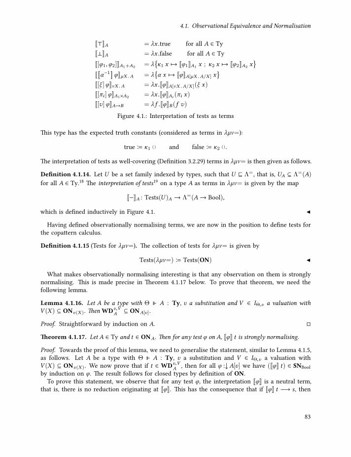
4.1. Observational Equivalence and Normalisation
J⊤KA = λx .true for all A ∈ TyJ⊥KA = λx .false for all A ∈ TyJ[ϕ1,ϕ2]KA1+A2= λ
κ1 x 7→ Jϕ1KA1
x ; κ2 x 7→ Jϕ2KA2x
J[α−1] ϕKµX .A = λα x 7→ JϕKA[µX .A/X ] x
J[ξ ]ϕKνX .A = λx .JϕKA[νX .A/X ](ξ x)J[πi ]ϕKA1×A2
= λx .JϕKAi (πi x)J[v]ϕKA→B = λ f .JϕKB(f v)Figure 4.1.: Interpretation of tests as terms
This type has the expected truth constants (considered as terms in λµν=):
true B κ1 ⟨ ⟩ and false B κ2 ⟨ ⟩.
The interpretation of tests as well-covering (Definition 3.2.29) terms in λµν= is then given as follows.
Definition 4.1.14. Let U be a set family indexed by types, such that U ⊑ Λ=, that is, UA ⊆ Λ=(A)
for all A ∈ Ty.18 The interpretation of tests19 on a type A as terms in λµν= is given by the map
J−KA : Tests(U )A → Λ=(A→ Bool),
which is defined inductively in Figure 4.1.
Having defined observationally normalising terms, we are now in the position to define tests forthe copattern calculus.
Definition 4.1.15 (Tests for λµν=). The collection of tests for λµν= is given by
Tests(λµν=) B Tests(ON)
What makes observationally normalising interesting is that any observation on them is stronglynormalising. This is made precise in Theorem 4.1.17 below. To prove that theorem, we need thefollowing lemma.
Lemma 4.1.16. Let A be a type with Θ ⊩ A : Ty, υ a substitution and V ∈ IΘ,υ a valuation withV (X ) ⊆ ONυ(X ). Then WDυ,V
A ⊆ ONA[υ].
Proof. Straightforward by induction on A.
Theorem 4.1.17. Let A ∈ Ty and t ∈ ONA. Then for any test ϕ on A, JϕK t is strongly normalising.
Proof. Towards the proof of this lemma, we need to generalise the statement, similar to Lemma 4.1.5,as follows. Let A be a type with Θ ⊩ A : Ty, υ a substitution and V ∈ IΘ,υ a valuation withV (X ) ⊆ ONυ(X ). We now prove that if t ∈ WDυ,V
A , then for all ϕ :↓A[υ] we have (JϕK t) ∈ SNBoolby induction on ϕ. The result follows for closed types by definition of ON.
To prove this statement, we observe that for any test ϕ, the interpretation JϕK is a neutral term,that is, there is no reduction originating at JϕK. This has the consequence that if JϕK t −→ s , then
83

Chapter 4. Observations
either s = JϕK t ′ with t −→ t ′, or JϕK t ≻ s . Since t ∈ SN by Lemma 4.1.5, we thus have that anyreduction sequence of JϕK t towards a normal form s is of the form
JϕK t JϕK t ′ ≻ s ′ s .
Using this property, all cases of the induction are straightforward, except for the case of least fixedpoint types. Thus, we focus on this case: Suppose we are given a test
[α−1
]ϕ with ϕ :↓A[µX .A/X ].
We define S ⊆ Λ=µX .A by
S =t ∈WDυ,V
µX .A
q[α−1
]ϕyt ∈ SN
,
and show WDυ,VµX .A ⊆ S . To prove this, we use the fixed point property of WDυ,V
µX .A. Thus, wehave to show Ψυ,V
A (S) ⊆ S . To this end, let t ∈ Ψυ,VA (S), leaving us with having to prove thatq[
α−1]ϕyt ∈ SN. By the property we mentioned in the beginning, we haveq[
α−1]ϕyt
q[α−1
]ϕy(α t ′) ≻ JϕK t ′. (4.3)
Recall that
Ψυ,VA (S) =
s (∃s ′. s α s ′) ∧
(∀s ′. (s α s ′) =⇒ s ′ ∈WDυ[µX .A/X ],V [X 7→S ]
A
).
From this and (4.3), we obtain t ′ ∈ WDυ[µX .A/X ],V [X 7→S ]A . By Lemma 4.1.16, we can apply the
induction hypothesis and get JϕK t ′ ∈ SN. Thus,q[α−1
]ϕyt ∈ SN by the above-mentioned property.
Since this holds for any t ∈ S , we have Ψυ,VA (S) ⊆ S .
Let us illustrate how to use Theorem 4.1.17 to show that a certain stream term is not observationallynormalising. This shows that we cannot compute a stream from that term, thereby showing thatthe stream term is not productive.
Example 4.1.18. Let x and even be given by
x : Natω
x .hd = 1
x .tl = even x
even : Natω → Natω
(even s).hd = hd s(even s).tl = even (s .tl.tl)
(4.4)
To see that x is not observationally normalising, we apply the evaluation context e = ·.tl.tl.hd to xand find that
e[x ] = x .tl.tl.hd −→ (even x).tl.hd −→ (even (x .tl.tl)).hd −→ x .tl.tl.hd = e[x ].
Hence, there is a diverging reduction sequence starting at e[x ], from which we get by Theorem 4.1.17that x is not in ON by using the test [tl] [tl] [hd]⊤, where the modalities [hd] and [tl] are defined inthe obvious way.
Recall that we defined the interpretation of stream terms as functions x† : N → N iteratively byx†(0) = n for x .hd ≡ n and x†(k + 1) = (x .tl)†(k). Note that the divergence of e[x ] implies thatthere is no natural number n ∈ N, such that e[x ] ≡ n. This in turn means that we cannot produce thevalue of x†(2), hence we cannot construct x† by successively computing head and tail of x . We saythat x is not productive, see [End+10; EH11]. If we interpret (4.4) as a system of stream differentialequations, then there is no unique solution for the variable x in (4.4), cf. [HKR17, Sec. 8.4].
84
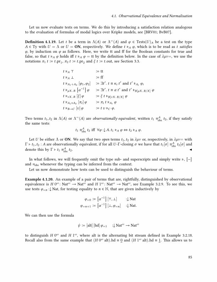
4.1. Observational Equivalence and Normalisation
Let us now evaluate tests on terms. We do this by introducing a satisfaction relation analogousto the evaluation of formulas of modal logics over Kripke models, see [BRV01; BvB07].
Definition 4.1.19. Let t be a term in Λ(A) or Λ=(A) and ϕ ∈ Tests(U )A be a test on the typeA ∈ Ty with U = Λ or U = ON, respectively. We define t ⊨A ϕ, which is to be read as t satisfiesϕ, by induction on ϕ as follows. Here, we write tt and ff for the Boolean constants for true andfalse, so that t ⊨A ϕ holds iff t ⊨A ϕ = tt by the definition below. In the case of λµν=, we use thenotations π1 t B t .pr1, π2 t B t .pr2 and ξ t B t .out, see Section 3.3.
t ⊨A ⊤ B ttt ⊨A ⊥ B fft ⊨A1+A2
[ϕ1,ϕ2] B ∃t ′. t ≡ κi t ′ and t ′ ⊨Ai ϕi
t ⊨µX . B[α−1
]ϕ B ∃t ′. t ≡ α t ′ and t ′ ⊨B[µX . B/X ] ϕ
t ⊨νX . B [ξ ]ϕ B ξ t ⊨B[νX . B/X ] ϕ
t ⊨A1×A2[πi ]ϕ B πi t ⊨Ai ϕ
t ⊨B→C [v]ϕ B t v ⊨C ϕ.
Two terms t1, t2 in Λ(A) or Λ=(A) are observationally equivalent, written t1 ≡Aobs t2, if they satisfythe same tests:
t1 ≡Aobs t2 iff ∀ϕ :↓A. t1 ⊨A ϕ ⇔ t2 ⊨A ϕ.
Let U be either Λ or ON. We say that two open terms t1, t2 in λµν or, respectively, in λµν= withΓ ⊢ t1, t2 : A are observationally equivalent, if for all U -Γ-closing σ we have that t1[σ ] ≡Aobs t2[σ ] anddenote this by Γ ⊢ t1 ≡Aobs t2.
In what follows, we will frequently omit the type sub- and superscripts and simply write ⊨, J−Kand ≡obs whenever the typing can be inferred from the context.
Let us now demonstrate how tests can be used to distinguish the behaviour of terms.
Example 4.1.20. An example of a pair of terms that are, rightfully, distinguished by observationalequivalence is H 0ω : Natω → Natω and H 1ω : Natω → Natω , see Example 3.2.9. To see this, weuse tests ϕ=n :↓Nat, for testing equality to n ∈ N, that are given inductively by
ϕ=0 B[α−1
][⊤,⊥] :↓Nat
ϕ=n+1 B[α−1
][⊥,ϕ=n ] :↓Nat.
We can then use the formula
ψ B [alt] [hd]ϕ=1 :↓Natω → Natω
to distinguish H 0ω and H 1ω , where alt is the alternating bit stream defined in Example 3.2.18.Recall also from the same example that (H 0ω alt).hd ≡ 0 and (H 1ω alt).hd ≡ 1. This allows us to
85

Chapter 4. Observations
show that H 0ω does not satisfy ψ , while H 1ω does satisfy ψ , as we have
H 0ω ⊨ [alt] [hd]ϕ=1 ⇐⇒ H 0ω alt ⊨ [hd]ϕ=1
⇐⇒ (H 0ω alt).hd ⊨ ϕ=1
⇐⇒ 0 ⊨[α−1
][⊥,ϕ=0] by (H 0ω alt).hd ≡ 0
⇐⇒ κ1 ⟨ ⟩ ⊨ [⊥,ϕ=0]
⇐⇒ ⟨⟩ ⊨ ⊥and
H 1ω ⊨ [alt] [hd]ϕ=1 ⇐⇒ · · · ⇐⇒ 1 ⊨ ϕ=1 ⇐⇒ · · · by (H 1ω alt).hd ≡ 1
⇐⇒ ⟨⟩ ⊨ ⊤.
So the terms H 0ω and H 1ω are distinguished by the test ψ .
After having seen an example of how to distinguish terms, let us now consider an example wherewe actually prove that two terms are observationally equivalent. This is typically done by inductionon tests.
Example 4.1.21. Recall that we gave in Example 3.2.7 another unit type 1′ = νX .X with a canonicalinhabitant ⟨ ⟩′. We now show that this term is actually unique up to observational equivalence. Thisrequires us to show for all terms t : 1′ that t ≡obs ⟨ ⟩′, which means by definition of observationalequivalence that we have to show for all tests ϕ ∈ Tests(λµν=)1′ that t ⊨ ϕ iff ⟨ ⟩′ ⊨ ϕ.
We proceed by induction on ϕ to prove for all terms t : 1′ that t ⊨ ϕ iff ⟨ ⟩′ ⊨ ϕ. Note thatthe term t is universally quantified in the induction hypothesis. Let t : 1′ be a term. In thebase case, where either ϕ = ⊤ or ϕ = ⊥, we trivially have t ⊨ ϕ ⇐⇒ ⟨⟩′ ⊨ ϕ. For theinduction step, ϕ is of the form ϕ = [ξ ]ψ with ψ ∈ Tests(λµν=)1′ . Since ⟨ ⟩′.out ≡ ⟨ ⟩′, see theopening discussion of Section 3.2.2, ⟨ ⟩′ ⊨ [ξ ]ψ ⇐⇒ ⟨⟩′ ⊨ ψ . Applying the induction hypothesisto ψ , we have t .out ⊨ ψ ⇐⇒ ⟨⟩′ ⊨ ψ . Thus, by definition of the satisfaction relation, we havet ⊨ [ξ ]ψ ⇐⇒ ⟨⟩′ ⊨ [ξ ]ψ , hence t ⊨ ϕ ⇐⇒ ⟨⟩′ ⊨ ϕ. So by induction, t and ⟨ ⟩′ satisfy the same testsϕ, thus are observationally equivalent.
At this point, a reader versed in the area of transition systems, coalgebras and such might wonderabout the relation of observational equivalence to bisimilarity. Indeed, it would be natural to view ⟨ ⟩′
as a single state transition system and prove that any other term of type 1′ is bisimilar to that system.The hope would then be that such a proof corresponds to showing that the term is observationallyequivalent to ⟨ ⟩′. In Section 5.1, we will show that one can define a general notion of bisimilarityon terms of all inductive-coinductive types, which coincides with observational equivalence.
Another point of interest might be whether it is possible to automatically prove that two termsare observationally equivalent. In fact, if there are no terms of function type involved, like inExample 4.1.21, then observational equivalence is decidable. One might call the function-free frag-ment of λµν= the data fragment, as we cannot carry out any computations, thus only constructdata, in that fragment. However, if we include functions, then observational equivalence becomesundecidable. We discuss this in detail in Section 5.3.
The following example illustrates a, perhaps surprising, effect of the restriction to observationallynormalising function arguments in the definition of observational normalisation itself: There is awell-defined function from the empty type 0 to any type A.
86

4.1. Observational Equivalence and Normalisation
Example 4.1.22. Recall the empty type from Example 3.1.2 was given by 0 = µX .X . We can givefor each type A a function E0A : 0→ A from 0 into A by20
E0A B rletf : 0→ A =
· (α x) 7→ f x
in f .
Note that there is no observationally normalising inhabitant of 0. This can be proved either bycontradiction to Lemma 4.1.5, or directly by induction. Since the latter is more elegant, let us provethat ON0 = ∅ by induction. To this end, recall that ON0 = µU .Ψ
(),εX (U ). Thus, we can prove
ON0 = ∅ by showing Ψ(),εX (∅) ⊆ ∅. Suppose now that s ∈ Ψ
(),εX (∅), thus there is an s ′ with
s α s ′ and s ′ ∈ ∅. This means, however, that there is no such s ′ and thus also no such s . Hence,Ψ
(),εX (∅) and ON0 are empty, as claimed. Since ON0 is empty and there are no reduction possible
on E0A, we have that E0A ∈ ON0→A.
Recall that we have defined an interpretation J−K of tests as terms of type A → Bool in λµν=.One might reasonably expect that this interpretation coincides with the satisfaction relation, inthe sense that for all tests and terms JϕK ≡ true iff t ⊨ ϕ. However, there is a subtle differenceon non-terminating terms: Let A be a type and put ϕ =
[α−1
]⊤, so that ϕ is a test on µX .A.
Recall that we defined in Example 3.2.21 a term ΩµX .A that only admits reduction steps of the formΩµX .A −→ ΩµX .A. This means then that neither JϕK(ΩµX .A) ≡ true nor JϕK(ΩµX .A) ≡ false. Onthe other hand, we have ΩµX .A ⊨ ϕ ⇐⇒ ∃t ′.ΩµX .Aα t ′ and t ′ ⊨ ⊤. Since no such t ′ exists, weconclude that ΩµX .A ⊭ ϕ. So the difference between the evaluation of JϕK(t) and t ⊨ ϕ lies in thefact that the former requires that there must be a way to reduce JϕK(t) to true or false. We capturethis situation in the following proposition.
Proposition 4.1.23. If t ∈ Λ=(A) and ϕ :↓A, such that JϕK(t) has a normal form, then
JϕK(t) ≡ true iff t ⊨ ϕ.
Proof. This follows by an easy induction on ϕ.
To put the above discussion into broader terms, if we accept the principle of excluded middle,then for all tests ϕ :↓A
∀t ∈ Λ=(A). t ⊨ ϕ ∨ t ⊭ ϕ.The example above shows however that in general ¬(∀t ∈ Λ=(A). JϕK(t) ≡ true ∨ JϕK(t) ≡ false).More generally, we can evaluate tests by using J−K only on observationally normalising terms,whereas on non-normalising terms J−K cannot assign a definite truth value to a test.
We finish this section by collecting some properties of observational equivalence. First, we showthat the definition of observational equivalence of open terms makes sense.
Lemma 4.1.24. For all x : A ⊢ ti : B with i = 1, 2, we have both in λµν and λµν=
x : A ⊢ t1 ≡Bobs t2 ⇔ λx .t1 ≡A→Bobs λx .t2 (4.5)
Proof. Since we have a common notation for function application and abstraction in both calculi,we give the proof independent of the calculus at hand. Let us write ri = λx .ti .
87

Chapter 4. Observations
’⇒’ We need to show that r1 and r2 satisfy the same tests ϕ. If ϕ = ⊤ or ϕ = ⊥, this is trivial. Ifϕ = [v]ψ , we have by assumption
r1 ⊨ ϕ ⇐⇒ t1[v/x ] ⊨ ψ ⇐⇒ t2[v/x ] ⊨ ψ ⇐⇒ r2 ⊨ ϕ
’⇐’ Let U be either Λ or ON. To show that t1 ≡obs t2, we need to show that t1[σ ] ≡Bobs t2[σ ] forevery U -(x : A)-closing substitution σ . That is to say we need to show t1[v/x ] ≡Bobs t2[v/x ]for every v ∈ U . But this follows immediately, as for every test ψ on B, we have
t1[v/x ] ⊨ ψ ⇐⇒ r1 ⊨ [v]ψ ⇐⇒ r2 ⊨ [v]ψ ⇐⇒ t2[v/x ] ⊨ ψ ,
just as for the other direction of the lemma.
The next lemma states a number of properties of that we will need frequently.
Lemma 4.1.25. Observational equivalence ≡obs has the following properties.
(i) Substitutivity: Given terms r ∈ ONx :AB and t1, t2 ∈ ONA such that t1 ≡Aobs t2, we have that
r [t1/x ] ≡Bobs r [t2/x ].
(ii) ≡obs is a congruence on ON, that is, ≡obs is an equivalence relation on ON and fulfils substitutivityas in (i), see [Pit04, Def. 7.5.1].
(iii) If t1 ≡Aobs t2, then for all f with ⊢ f : A→ B we have f t1 ≡Bobs f t2.
(iv) ≡obs strictly contains convertibility (i.e., ≡ ⊂ ≡obs).
(v) ≡obs is extensional for terms of function type: if t1, t2 : A→ B and t1v ≡obs t2v for all v : A in ON,then t1 ≡obs t2.
(vi) ≡obs contains η-equivalence: λx .tx ≡obs t , x < fv(t).
Most of these properties are straightforward to prove, only substitutivity (i) requires a bit morework. The proof uses the following technical lemma.
Lemma 4.1.26. Let s ∈ ONx :AB and let t ∈ ONA. For all tests ϕ :↓ B with s[t/x ] ⊨ ϕ there are tests
ψ1, . . . ,ψn on A such that
(i) t ⊨ ψi for all 1 ≤ i ≤ n and
(ii) for all t ′ ∈ ONA, if t ′ ⊨ ψi for all 1 ≤ i ≤ n, then s[t ′/x ] ⊨ ϕ.
This lemma states that we can find for each computation that s can make, formulas that characteriseinputs to s that lead to the same output as t . One can read this as a continuity property of s , inthe sense that finite observations on s[t/x ] only depend on finite observations on t . We will not gointo this further here, but it is discussed in [BH16].
88

4.1. Observational Equivalence and Normalisation
Proof of Lemma 4.1.26. To prove the statement of the lemma, we need to generalise it a bit. Thisgeneralisation becomes easier, if we use conjunctive tests, that is, tests that may contain conjunctions.Given tests ϕ1,ϕ2 : A, their conjunction ϕ1 ∧ϕ2 is satisfied by t : A if t ⊨ ϕi for both i = 1 and i = 2.Conjunctive tests allow us to simplify the formulation of Lemma 4.1.26 by replacing ψ1, . . . ,ψn byψ = ψ1 ∧ · · · ∧ψn .
More generally, we set out to prove the following. Let f ∈ ONΓA and let τ ∈ Subst(ON,Γ). For
all tests ϕ :↓A with f [τ ] ⊨ ϕ there are conjunctive tests ψx x ∈dom(Γ) such that(i) τ (x) ⊨ ψx for all x ∈ dom(Γ) and
(ii) for all σ ∈ Subst(ON,Γ), if σ(x) ⊨ ψx for all x ∈ dom(Γ), then f [σ ] ⊨ ϕ.We only sketch the proof of this generalised property. Since f is in ONΓ
A, JϕK(f [τ ]) is stronglynormalising, thus there is a finite reduction sequence JϕK(f [τ ]) N to a normal form. We obtainthe family ψx by induction on this reduction sequence. In this induction, two cases have to bedistinguished: either τ (x) is contracted within an evaluation context e , in which case ψx is extendedby the modalities given by e , or τ (x) is used as a function argument in a contraction. In the lattercase, we reduce the corresponding function to λD or a symbol д, and extend ψx by the pattern ofD or д that matched τ (x).21
Proof of Lemma 4.1.25. (i) To show that r [t1/x ] ≡obs r [t2/x ], we show that both terms simultan-eously satisfy any test ϕ : B.First, assume that r [t1/x ] ⊨ ϕ. Lemma 4.1.26 gives us that for τ = [t1/x ] there are testsψ1, . . . ,ψn on A, such that ∀1 ≤ i ≤ n. t1 ⊨ ψi and if ∀1 ≤ i ≤ n. t2 ⊨ ψi , then r [t2/x ] ⊨ ϕ. Sincet1 ≡obs t2, both terms simultaneously satisfy all the ψi , thus r [t2/x ] ⊨ ϕ.Conversely, r [t2/x ] ⊨ ϕ implies, in the same way, that r [t1/x ] ⊨ ϕ. Summarising, the termsr [t1/x ] and r [t2/x ] satisfy the same tests, hence are observationally equivalent.
(ii) This follows immediately from ≡ being an equivalence relation and from (i).
(iii) This is just the combination of (i) and Lemma 4.1.24.
(iv) The inclusion is proved by induction on tests. It is strict by appealing to item (v): For instance,the terms λx . x and λ
· (α x) 7→ x
are not convertible but they are observationally equivalent
by extensionality.
(v) Trivially by the shape of tests on A→ B.
(vi) Let t : A → B be a term with x < fv(t). For every v ∈ ONA, we have (λx .(t x))v ≡ t v andhence by (iv) and (v) the equivalence λx .(t x) ≡obs t follows.
The last property of ≡obs we record is that the equational theory ≡obs is consistent.Definition 4.1.27 (cf. [Bar85, Def. 2.1.30]). An equational theory for a family UAA∈Ty is a family≈ of equivalence relations ≈A ⊆ UA ×UA. The equational theory is said to be consistent, if there isA ∈ Ty and s, t ∈ UA with s 0A t .Proposition 4.1.28. The equational theory ≡obs is consistent both for Λ and Λ=.
Proof. The terms true, false : Bool are not observationally equivalent, as they are distinguishable bythe test [⊤,⊥]. Hence ≡obs is consistent.
89
Chapter 4. Observations
4.2. Category Theoretical Properties of λµν and λµν=We have now seen two different calculi for programming with mixed inductive-coinductive types,and we introduced a notion of program equivalence that is based on program observations for thesecalculi. Moreover, we defined what it means for a program in the calculus λµν= to be observationallynormalising, using again the same notion of program observation. Basing program equivalence andobservational normalisation on observations is an intuitive approach, but we need to show how thesenotions relate to properties that occur elsewhere in the description of program behaviour. Specifically,we want to relate here to the usual category theoretical definition of inductive-coinductive objectsin terms of unique mapping properties. We proceed in two steps to clarify the relation. First, weintroduce in Section 4.2.1 the so-called classifying category for each of the calculi. Then we show thatthe classifying categories indeed admit to some extent the categorical structures that are suggestedby the types. For instance, greatest fixed point types are weakly final coalgebras.
The problem with classifying categories is that we are trying to force the calculi into a cloakthat does not really fit them. Just to name one major issue: the action of types on terms, given inDefinition 3.1.9, looks like the definition of a functor on the classifying categories but it really isnot. Thus we are not even able to, for instance, form a category of coalgebras for open types.
We overcome these issues in a second step, where we refine the classifying categories by (1) re-stricting the attention to only observationally normalising terms in the classifying category forλµν=, and (2) augmenting the classifying categories with observational equivalence as 2-categoricalstructure. The first step is important to properly classify inductive types (sums and least fixedpoints), since non-termination leads to inhabitants of inductive types on which no observation ispossible, see the discussion before Proposition 4.1.23. Through the second step we obtain a precisecategorical classification of the types, in the sense that the action of a type on terms turns out tobe a pseudo-functor and largest fixed point types are pseudo-final coalgebras.
One might now raise the objection to the 2-categorical approach that we could just take a quotientof the classifying 2-categories, which allows us to drop the prefix “pseudo” everywhere. However,besides violating the abstract “principle of equivalence” [nLa16], we also lose some information byforming a quotient category: we cannot distinguish anymore between term equivalences arisingfrom computations and those stemming from observational equivalence.
4.2.1. Simple Classifying CategoriesThe goal of this section is to describe the categorical structure that arises from the type structureof the calculi λµν and λµν=. We begin by identifying properties of calculi for which we are able togive classifying categories22, see Definition 4.2.2.
Definition 4.2.1. Let U be a set. We assume that there is a judgement of the form
x : A ⊢ t : B,
which is a relation between contexts x : A and elements t ∈ U, where A and B are types as inDefinition 3.1.1. The set U together with the relation ⊢ is called a classifiable calculus, if
1. Projection holds: TeVar ⊆ U, and for all x ∈ TeVar, the judgement x : A ⊢ x : A is valid;
2. Substitution exists: for every t , s ∈ U and x ∈ TeVar, there is an element t [s/x ] ∈ U;
90

4.2. Category Theoretical Properties of λµν and λµν=
3. Substitution preserves typing: if x : B ⊢ t : C and x : A ⊢ s : B, then x : A ⊢ t [s/x ] : C;
4. Substitution preserves identities: For all t , s ∈ U and x ∈ TeVar, x [t/x ] = t and t [x/x ] = t ;
5. Substitution lemma holds: For all t , s ∈ U and x ∈ TeVar,
t [s[r/x ]/x ] = t [s/x ][r/x ]. (4.6)
Given a classifiable calculus, we will refer to the elements of U as terms.
A classifiable calculus allows us, as the name suggests, to construct its classifying category.23
Definition 4.2.2. Let U be a classifiable calculus. We denote by Cℓs (U) the simple classifyingcategory of U, given as follows.
Cℓs (U) =
objects: Types Amorphisms: t : A→ B is a term t ∈ U with x : A ⊢ t : B
An identity morphism A→ A is given by x : A ⊢ x : A and composition is defined by substitution:t s = t [s/x ]. That the composition is well-defined follows from type preservation. The identity lawis immediate by t [x/x ] = t and x [t/x ] = t , whereas associativity is given by (4.6).
Lemma 4.2.3. Both Λ and Λ= are classifiable, thus their respective simple classifying categories Cℓs (Λ)and Cℓs (Λ=) exist.
Proof. The judgement Γ,x : A ⊢ x : A is immediate by projection in both calculi. Equation (4.6) isproved by a simple but tedious induction on terms, just like the other conditions.
This description of the calculi allows us to state Theorem 3.3.4 more precisely.
Proposition 4.2.4. The map (−) : Λ→ Λ= extends to a functor Cℓs (Λ)→ Cℓs (Λ=).
Proof. We define (−) on types to be the identity. Then, by the type preservation in Theorem 3.3.4,we have that for a morphism (a term) t : A→ B that t : A → B. So it remains to prove thatthe encoding preserves identities and composition. The former is immediate, since x = x . Thatcomposition is preserved means that s[t/x ] = s[t/x ], which is proved by induction on s .
To establish further categorical structure on the simple classifying categories, we need to takesome term equivalences into account.
Definition 4.2.5. Suppose U is a classifiable calculus with an equivalence relation ≡ on terms thatrespects substitution: if t ≡ t ′ and s ≡ s ′, then t [s/x ] ≡ t ′[s ′/x ]. Suppose further that ≡ is typecorrect, that is, for all Γ ⊢ t : A and s , if t ≡ s then Γ ⊢ s : A. Then the simple classifying categorymodulo computations Cℓ≡s (U) is the quotient category Cℓs (U)/≡, see Section 2.2.
Many categorical constructions are described through universal mapping property (UMP). For in-stance, the Cartesian product of two objects A1 and A2 is given by an object A1 × A2 and twoprojections πi : A1 × A2 → Ai , such that for all f1 : C → A1 and f2 : C → A2 there exists a uniqueд : C → A1 × A2 with πi д = fi . In the context of type theory one tries to model these UMPs
91
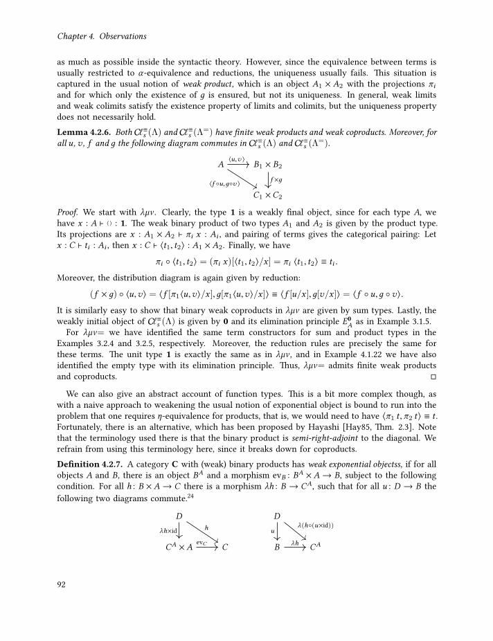
Chapter 4. Observations
as much as possible inside the syntactic theory. However, since the equivalence between terms isusually restricted to α-equivalence and reductions, the uniqueness usually fails. This situation iscaptured in the usual notion of weak product, which is an object A1 × A2 with the projections πiand for which only the existence of д is ensured, but not its uniqueness. In general, weak limitsand weak colimits satisfy the existence property of limits and colimits, but the uniqueness propertydoes not necessarily hold.Lemma 4.2.6. Both Cℓ≡s (Λ) and Cℓ≡s (Λ=) have finite weak products and weak coproducts. Moreover, forall u, v , f and д the following diagram commutes in Cℓ≡s (Λ) and Cℓ≡s (Λ=).
A B1 × B2
C1 ×C2
⟨u,v ⟩
⟨f u,дv ⟩ f ×д
Proof. We start with λµν . Clearly, the type 1 is a weakly final object, since for each type A, wehave x : A ⊢ ⟨ ⟩ : 1. The weak binary product of two types A1 and A2 is given by the product type.Its projections are x : A1 × A2 ⊢ πi x : Ai , and pairing of terms gives the categorical pairing: Letx : C ⊢ ti : Ai , then x : C ⊢ ⟨t1, t2⟩ : A1 ×A2. Finally, we have
πi ⟨t1, t2⟩ = (πi x)[⟨t1, t2⟩/x ] = πi ⟨t1, t2⟩ ≡ ti .Moreover, the distribution diagram is again given by reduction:
(f × д) ⟨u,v⟩ = ⟨f [π1⟨u,v⟩/x ],д[π1⟨u,v⟩/x ]⟩ ≡ ⟨f [u/x ],д[v/x ]⟩ = ⟨f u,д v⟩.It is similarly easy to show that binary weak coproducts in λµν are given by sum types. Lastly, theweakly initial object of Cℓ≡s (Λ) is given by 0 and its elimination principle E0A as in Example 3.1.5.
For λµν= we have identified the same term constructors for sum and product types in theExamples 3.2.4 and 3.2.5, respectively. Moreover, the reduction rules are precisely the same forthese terms. The unit type 1 is exactly the same as in λµν , and in Example 4.1.22 we have alsoidentified the empty type with its elimination principle. Thus, λµν= admits finite weak productsand coproducts.
We can also give an abstract account of function types. This is a bit more complex though, aswith a naive approach to weakening the usual notion of exponential object is bound to run into theproblem that one requires η-equivalence for products, that is, we would need to have ⟨π1 t ,π2 t⟩ ≡ t .Fortunately, there is an alternative, which has been proposed by Hayashi [Hay85, Thm. 2.3]. Notethat the terminology used there is that the binary product is semi-right-adjoint to the diagonal. Werefrain from using this terminology here, since it breaks down for coproducts.Definition 4.2.7. A category C with (weak) binary products has weak exponential objectss, if for allobjects A and B, there is an object BA and a morphism evB : BA × A→ B, subject to the followingcondition. For all h : B × A→ C there is a morphism λh : B → CA, such that for all u : D → B thefollowing two diagrams commute.24
D
CA ×A C
hλh×idevC
D
B CA
uλ(h(u×id))
λh
92

4.2. Category Theoretical Properties of λµν and λµν=
Lemma 4.2.8. Both Cℓ≡s (Λ) and Cℓ≡s (Λ=) have weak exponential objects.
Proof. For Cℓ≡s (Λ) the exponential object BA for types A and B is given by the function space A→ Band the evaluation map evB by
x : BA ×A ⊢ (π1 x) (π2 x) : B.
Let t : B ×A→ C , that is, x : B ×A ⊢ t : C . We define λt : B → CA to be the term
x : B ⊢ λy. t [⟨x ,y⟩/x ] : A→ C .
For terms x : D ⊢ u : B and x : D ⊢ v : A we now haveevC ⟨λt u,v⟩ = ((π1 x) (π2 x))[⟨λt u,v⟩/x ]
≡ (λt u)v= ((λy. t [⟨x ,y⟩)/x ])[u/x ])v= (λy. t [⟨u,y⟩/x ])v≡ t [⟨u,v⟩/x ]= t ⟨u,v⟩
andλ(t (u × id)) ≡ λ(t ⟨u π1,π2⟩)
= λ(t [⟨u[π1 x/x ],π2 x⟩/x ])= λy. (t [⟨u[π1 x/x ],π2 x⟩/x ])[(x ,y)/x ]≡ λy. (t [⟨u[x/x ],y⟩/x ])= λy. (t [⟨u,y⟩/x ])= (λy. (t [⟨x ,y⟩/x ]))[u/x ]= λt u .
Thus Cℓ≡s (Λ) has weak exponential objects. That Cℓ≡s (Λ=) also has weak exponentials follows bythe same reasoning and using the notations introduced in Example 3.2.6.
For the following proposition we need to relax our understanding of what algebras and coalgebrasare. Recall from Section 2.5 that an initial algebra for a functor F : C→ C is a morphism FA→ Afor some object A, such that for all algebras FB → B there is a unique homomorphism A→ B. Theconcept of a final coalgebra is defined dually. We would like to understand fixed point types inthese terms. Just as in Lemma 4.2.6, we can drop the uniqueness constraint for the homomorphismto obtain a notion of weakly initial algebras and weakly final coalgebras. However, already the veryusage of functors in the definition of (co)algebras poses a problem because the action of types onterms that we gave in Definition 3.1.9 does not satisfy the laws of a functor. Thus, fixed point typesdo not have a (co)algebra structure for a functor F in the usual sense, rather we can only require Fto be a map on objects and morphisms.
Definition 4.2.9. A pre-functor F : C→ D between categories C and D is a map that sends everyobject X ∈ obD to an object F (X ) ∈ obD, and every morphism f : X → Y in C to a morphismF (f ) : F (X )→ F (Y ) in D.
93

Chapter 4. Observations
Pre-functors are the weakest possible mapping between categories. However, since they neitherpreserve identities nor composition, there is no good general theory for pre-functors. The reasonwhy we are introducing them here nevertheless is to have a language for organising the propertiesof fixed point types. By abuse of language, we will also talk about algebras, coalgebras and theirhomomorphisms, even if we are only given a pre-functor instead of a functor, cf. Definition 2.5.3.
Definition 4.2.10. Let F : C → C be a pre-functor. A weakly final coalgebra for F is a morphismc : X → FX in C, such that for every coalgebra d : Y → FY there is a coalgebra homomorphismf : Y → X from d to c . Weakly initial algebras for F are defined dually.
Lemma 4.2.11. Let X ⊩ T : Ty, that is, let T be a type with a free type variable X , see Definition 3.1.1.Then T gives rise to pre-functors Cℓ≡s (Λ)→ Cℓ≡s (Λ) and Cℓ≡s (Λ=)→ Cℓ≡s (Λ=) by putting
T (A) B T [A] = T [A/X ] and T (t) B T [λx .t ] x ,
usingT [−] as defined in Definition 3.1.9. Moreover, there is a weakly initial algebra δ : T (µX .T )→ µX .Tand a weakly final coalgebraω : νX .T → T (νX .T ) both in Cℓ≡s (Λ) and Cℓ≡s (Λ=). This means that for anymorphisms a : T (A)→ A and c : A→ T (A) there are (not necessarily unique) morphisms a : µX .T → Aand c : A→ νX .T , such that the following two diagrams commute.
T (µX .T ) T (A)
µX .T A
δ
T (a)
a
a
A νX .T
T (A) T (νX .T )
c
c
ω
T (c)
Proof. To show that T gives rise to a map Cℓ≡s (Λ)→ Cℓ≡s (Λ) requires us to show that t ≡ s impliesT (t) ≡ T (s). This, in turn, follows from ≡ being a congruence and by a simple induction on T . Recallthat T (A) = T [A/X ], so that
x : T (µX .T ) ⊢ α x : µX .T and x : νX .T ⊢ ξ x : T (νX .T ),
and the algebra and coalgebra structures are thus given by δ B α x and ω B ξ x . Next, giveny : T (A) ⊢ a : A and y : A ⊢ c : T (A), as in the assumption, we can define the inductive extension of aby a B iterµX .T (y. a) y and the coinductive extension of c by c B coiterνX .T (y. c) y, thus obtaining
y : µX .T ⊢ a : A and y : A ⊢ c : νX .T .
Before we continue, let us briefly spell out the diagram for weakly final coalgebras in Cℓ≡s (Λ).Since morphisms in Cℓ≡s (Λ) are (equivalence classes) of terms with a free variable for the domain,we can picture the homomorphism diagram for c as follows.
A νX .T
T (A) T (νX .T )
y : A ⊢ coiterνX .T (y . c) y : νX .T
x : A ⊢ c : T (A) x : νX .T ⊢ ξ x : T (νX .T )
x : T (A) ⊢ T (coiterνX .T (y . c) y) : T (νX .T )
≡
94

4.2. Category Theoretical Properties of λµν and λµν=
That this homomorphism diagram commutes follows directly from the definition of conversion:
ω c = (ξ x)[coiterνX .T (y. c) y/x ]
= ξ (coiterνX .T (y. c) y)
≡ T [λy.(coiterνX .T (y. c) y)](c[y/y])
= T [λy.(coiterνX .T (y. c) y)] c
= T(coiterνX .T (λy.c) y
)[c/x ]
= T (c) c,
and analogously for µX .T .In Cℓs (Λ=) we find back exactly the same structure by putting
δ B α x and ω B x .out,
anda B rlet f : µX .T → A = · (α x) 7→ a[T (f x)/x ] in f x
c B rlet f : A→ νX .T = (· x).out 7→ T (f x)[c/x ] in f x .
That these are well-typed is checked as in Theorem 3.3.4. Note that the inductive extensions a andthe coinductive extensions c resemble the rewriting steps as given by contraction for iter and coiterin Definition 3.1.11. Hence that these are homomorphisms just follows as for λµν .
4.2.2. Classifying 2-CategoriesOn the one hand, we have given in Section 4.2.1 a category theoretical account of the computationalbehaviour of terms in the two calculi λµν and λµν=. On the other hand, we have described inSection 4.1 the observational behaviour of terms. The purpose of the present section is to mergethese two views. This is achieved by augmenting the classifying categories Cℓ≡s (Λ) and Cℓ≡s (Λ=)with a 2-categorical structure that encodes the information about observations. This allows us tocontrast the equality between morphisms in these categories, which relates terms with the samecomputational behaviour , and 2-cells between the morphisms, which relates terms with the sameobservational behaviour .
The 2-categories, which we obtain by adding 2-cells to the simple classifying categories, have“pseudo” instead of “weak” categorical structure. For instance, the product types do not just haveprojections πi and pairing, subject to the equations πi ⟨f1, f2⟩ = fi , but the pairing is additionallyunique up to isomorphism, see Definition 2.6.8. This stronger property allows us to show that theaction of types on terms gives rise to a pseudo-functor. Thus, we can form 2-categories of algebrasand coalgebras, whose pseudo-initial and, respectively, pseudo-final objects are given by fixed pointtypes.
When enhancing the results of Section 4.2.1, we will find that we get an even stronger resultthan just pseudo-structures. Note that in the definition of pseudo-products, Definition 2.6.8, wehave that for all fi : C → Ai there is an h : C → A1 × A2 with πi h fi . So there only needsto be an isomorphism between πi h and fi . However, we have shown in Lemma 4.2.6 that in the
95

Chapter 4. Observations
classifying categories there is a (not necessarily unique) h, such that π h = fi . We will call sucha structures pseudo-products with strict choice. These characterise precisely the interplay of thereduction relation of the calculi and observational equivalence.
We begin by casting this last discussion into definitions, thereby refining the definitions given inDefinition 2.6.8.
Definition 4.2.12. Let C be a 2-category. We say that C has finite pseudo-products with strict choice,if it has finite pseudo-products, see Definition 2.6.8, such that for all A1, A2 and fi : C → Ai thereis an h : C → A1 × A2 with πi h = fi , where πi : A1 × A2 → Ai are the projections of thepseudo-product. We denote this h by ⟨f1, f2⟩. Moreover, we have for all appropriate u, v , f , дthat (f × д) ⟨u,v⟩ = ⟨f u,д v⟩, cf. Lemma 4.2.6. Dually, C is said to have pseudo-coproductswith strict choice, if it has pseudo-coproducts, with injections κi : Ai → A1 + A2, such that forall morphisms fi : Ai → C , there is a morphism [f1, f2] : A1 + A2 → C with [f1, f2] κi = fi .Finally, pseudo-exponents with strict choice in C are pseudo-exponents, such that the two identitiesin Definition 4.2.7 are fulfilled.25
Let us now identify the concepts from Definition 4.2.12 in the calculi λµν and λµν=. To do that,we first need to enrich their classifying categories with a 2-categorical structure that representsobservational equivalence.
Lemma 4.2.13. There are 2-categories Cℓ≡s,obs(Λ) and Cℓ≡s,obs(ON), where26
Cℓ≡s,obs(Λ) B
objects: types Amorphisms: [t ]≡ : A→ B is the convertibility equivalence class of a term
t ∈ Λ with x : A ⊢ t : B2-cells: t ⇒ s exists iff t ≡obs s .
and
Cℓ≡s,obs(ON) Bobjects: types Amorphisms: [t ]≡ : A→ B is the convertibility equivalence class of a term t ∈ ONx :A
B
2-cells: t ⇒ s exists iff t ≡obs s .
Proof. The vertical composition of 2-cells in Cℓ≡s,obs(Λ) is just given by transitivity of observationalequivalence: If γ : r ⇒ s and ρ : s ⇒ t , then r ≡obs s and s ≡obs t . By transitivity we have r ≡obs t ,and thus there is a δ : r ⇒ t . Since 2-cells are unique in Cℓ≡s,obs(Λ), we can define ρ 1 γ = δ .
Horizontal composition arises in a situation like the following.
A B C
t
t ′
≡obss
s ′
≡obs
By (i) of Lemma 4.1.25 and the definition of observational equivalence on open terms we have
s[t/x ] ≡obs s[t ′/x ] ≡obs s ′[t ′/x ],
96
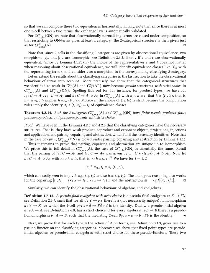
4.2. Category Theoretical Properties of λµν and λµν=
so that we can compose these two equivalences horizontally. Finally, note that since there is at mostone 2-cell between two terms, the exchange law is automatically validated.
For Cℓ≡s,obs(ON) we note that observationally normalising terms are closed under composition, sothat restricting to ON-terms gives at least a category. The 2-categorical structure is then given justas for Cℓ≡s,obs(Λ).
Note that, since 2-cells in the classifying 2-categories are given by observational equivalence, twomorphisms [s]≡ and [t ]≡ are isomorphic, see Definition 2.6.3, if only if s and t are observationallyequivalent. Since by Lemma 4.1.25.(iv) the choice of the representatives s and t does not matterwhen reasoning about observational equivalence, we will identify equivalence classes like [s]≡ withthe representing term s , and consider s as a morphism in the corresponding classifying 2-category.
Let us extend the results about the classifying categories in the last section to take the observationalbehaviour of terms into account. More precisely, we show that the categorical structures thatwe identified as weak in Cℓ≡s (Λ) and Cℓ≡s (Λ=) now become pseudo-structures with strict choice inCℓ≡s,obs(Λ) and Cℓ≡s,obs(ON). Spelling this out for, for instance, for product types, we have fort1 : C → A1, t2 : C → A2 and h : C → A1 ×A2 in Cℓ≡s,obs(Λ) with πi h ti that h ⟨t1, t2⟩, that is,πi h ≡obs ti implies h ≡obs ⟨t1, t2⟩. Moreover, the choice of ⟨t1, t2⟩ is strict because the computationrules imply the identity πi ⟨t1, t2⟩ = ti of equivalence classes.
Theorem 4.2.14. Both the 2-categories Cℓ≡s,obs(Λ) and Cℓ≡s,obs(ON) have finite pseudo-products, finitepseudo-coproducts and pseudo-exponents with strict choice.
Proof. We have seen in the Lemmas 4.2.6 and 4.2.8 that the classifying categories have the necessarystructures. That is, they have weak product, coproduct and exponent objects, projections, injectionsand application, and pairing, copairing and abstraction, which fulfil the necessary identities. Note thatin the case of λµν=, Cℓ≡s,obs(ON) is closed under pairing, copairing and abstraction by Lemma 4.1.11.
Thus it remains to prove that pairing, copairing and abstraction are unique up to isomorphism.We prove this in full detail in Cℓ≡s,obs(Λ), the case of Cℓ≡s,obs(ON) is essentially the same. Recallthat the pairing of t1 : C → A1 and t2 : C → A2 was given by x : C ⊢ ⟨t1, t2⟩ : A1 × A2. Now leth : C → A1 ×A2 with πi h ti , that is, πi h ≡obs ti .27 We have for i = 1, 2
πi h ≡obs ti ≡ πi ⟨t1, t2⟩,
which can easily seen to imply h ≡obs ⟨t1, t2⟩ and so h ⟨t1, t2⟩. The analogous reasoning also worksfor the copairing [t1, t2] = κ1 x 7→ t1 ; κ2 x 7→ t2 x and the abstraction λt = λy.t [⟨x ,y⟩/x ].
Similarly, we can identify the observational behaviour of algebras and coalgebras.
Definition 4.2.15. A pseudo-final coalgebra with strict choice is a pseudo-final coalgebra c : X → FX ,see Definition 2.6.9, such that for all d : Y → FY there is a (not necessarily unique) homomorphismd : Y → X for which the 2-cell φd : c d ⇒ Fd d is the identity. Dually, a pseudo-initial algebraa : FA→ A, see Definition 2.6.9, has a strict choice, if for every algebra b : FB → B there is a pseudo-homomorphism b : A→ B, such that the mediating 2-cell θb : b a ⇒ b Fb is the identity.
Next, we prove that for each type A the action of A on terms, see Definition 3.1.9, gives rise to apseudo-functor on the classifying categories. Moreover, we show that fixed point types are pseudo-initial algebras or pseudo-final coalgebras with strict choice for these pseudo-functors. These two
97

Chapter 4. Observations
results are proved my mutual induction, since pseudo-initial algebras and pseudo-final coalgebrasare used to define functors from fixed point types, and conversely, pseudo-functoriality is needed toobtain pseudo-initial algebras and pseudo-final coalgebras for smaller types.
We start the mutual induction by showing that the type action indeed gives a pseudo-functor.
Lemma 4.2.16. Let T be a type with X1, . . . ,Xn ⊩ T : Ty.28 If all fixed point types occurring in Tare pseudo-initial algebras and pseudo-final coalgebras, then the maps of categories associated with Tin Lemma 4.2.11 can be extended to pseudo-functors of arity n: T (−) :
(Cℓ≡s,obs(Λ)
)n → Cℓ≡s,obs(Λ) andT (−) :
(Cℓ≡s,obs(ON)
)n → Cℓ≡s,obs(ON).Proof. To show that that T (−) is a pseudo-functor, we need to extend T (−) to 2-cells and prove thatT (−) preserves identity morphisms and composition up to isomorphism, that is, up to observationalequivalence. First, recall that for a tuple #—
t of terms we defined T (#—t ) = T [
# —
λx . t ] x in Lemma 4.2.11.By the definition of the type action in Definition 3.1.9, we have that T [−] substitutes #—
t into anobservationally normalising context. Thus, if #—
t ≡obs#—
t ′ , we have by Lemma 4.1.25(i) that alsoT( #—t)≡obs T
( #—
t ′). This in turn means, that we can send a 2-cell in
(Cℓ≡s,obs(Λ)
)n , which says that allthe terms in #—
t and #—
t ′ are observationally equivalent, to the unique 2-cell in Cℓ≡s,obs(Λ) that expressesthat T
( #—t)and T
( #—
t ′)are observationally equivalent. So T also has a well-defined action on 2-cells.
It remains to prove that T fulfils the law of a pseudo-functor. We proceed by induction on T . Inthe base case T = Xi , we note that Xi [−] is the ith projection from the product category, hence apseudo-functor.
To prove the induction step, we need to show that for compound types T , T (−) is a pseudo-functor, provided that its components are pseudo-functors. Concretely, we need to show that thepseudo-functor laws hold for the compound types T1 +T2, T1 ×T2 and T1 → T2, provided the lawshold for T1 and T2. This is a routine calculation by using Theorem 4.2.14.
The case for fixed point types is essentially an adoption of the standard proof that the point-wiseexistence of final coalgebras gives rise to a functor [Kim10], but we have to replace equality betweenmorphisms by observational equivalence. We give the details for νX .T , the case for least fixed pointtypes is analogous. Consider the fixed point type νX .T . The induction hypothesis is in this casefor X1, . . . ,Xn ,X ⊩ T : Ty that T (−) :
(Cℓ≡s,obs(Λ)
)n+1 → Cℓ≡s,obs(Λ) is a pseudo-functor. Now let#—t :
#—A → #—
B be a morphism in(Cℓ≡s,obs(Λ)
)n . By Lem. 4.2.18 below, the pseudo-functors T ( #—A ,−)
and T (#—B ,−) of type Cℓ≡s,obs(Λ) → Cℓ
≡s,obs(Λ) have as pseudo-final coalgebras ξ #—
A and ξ #—B , and we
take (νX .T )(#—t ) to be the coinductive extension (Lemma 4.2.11) of
νT (#—A ,−)
ξ #—A−−→ T (#—A ,νT (
#—A ,−))
T (#—A , id)
−−−−−−→ T (#—B ,νT (
#—A ,−)),
cf. Definition 3.1.9. The pseudo-functor laws follow from uniqueness up to isomorphism of coin-ductive extensions on pseudo-final coalgebras, see Section 2.6.2.
In case of Cℓ≡s,obs(ON), one proceeds in exactly the same way, only that we have to use Proposi-tion 4.1.9.(i) to ensure that the functorial action of T is a morphism in Cℓ≡s,obs(ON).
The following technical lemma is used in the proof of Lemma 4.2.18. It allows us to construct foreach coalgebra c and each test ϕ on the unfolding of largest fixed point types, a “universal” term t
98

4.2. Category Theoretical Properties of λµν and λµν=
that cannot be distinguished from any homomorphism from c into the largest fixed point up to theobservation depth given by ϕ.
Lemma 4.2.17. Let T be a type with X ⊩ T : Ty.
1. For every coalgebra c : A → T [A] in one of the classifying 2-categories, every (observationallynormalising) term u : A and every test ϕ :↓T [νX .T ], there is a term t with x : A ⊢ t : T [νX .T ],such that for any T -coalgebra pseudo-homomorphism h : A→ νX .T from c to ω = ξ x , we have
t [u/x ] ⊨ ϕ ⇐⇒ (ξ h)[u/x ] ⊨ ϕ.
2. For every algebra a : T [A] → A in one of the classifying 2-categories, every (observationally nor-malising) term u : T [A] and every test ϕ :↓ A, there is x : T [µX .T ] ⊢ t : A, such that for anypseudo-homomorphism h : µX .T → A from δ = α x to a, we have
t [u/x ] ⊨ ϕ ⇐⇒ h[α u/x ] ⊨ ϕ.
Proof. We only sketch the proof of 1, the proof of 2 is given by duality. Since h is a pseudo-homomorphism, we have (ξ h)[u/x ] ⊨ ϕ ⇐⇒ (T [h] c)[u/x ] ⊨ ϕ hence it suffices to prove theexistence of a t with t [u/x ] ⊨ ϕ ⇐⇒ (T [h] c)[u/x ] ⊨ ϕ. We do this by proving the following.
For any sub-expression S of T ,29 any x : A ⊢ c ′ : T [A], any u ′ ∈ ONA and any test ψ :↓ S[νX .T ]there is x : A ⊢ t : S[νX .T ], such that for any T -coalgebra pseudo-homomorphism f from c ′ toω = ξ x the equivalence t [u ′/x ] ⊨ ψ ⇐⇒ (S[f ] c ′)[u ′/x ] ⊨ ψ holds. The result then follows bytaking c ′ = c and ψ = ϕ. The claim itself is proved by induction on ψ .
The following lemma is needed in the induction step for fixed points in the proof of Lem. 4.2.16.
Lemma 4.2.18. For any typeT withX ⊩ T : Ty, if the associated map of classifying categories defined inLemma 4.2.11 is a pseudo-functor, then δ : T (µX .T )→ µX .T is a pseudo-initial algebra andω : νX .T →T (νX .T ) a pseudo-final coalgebra with strict choice.
Proof. We already proved in Lemma 4.2.11 that δ and ω are weakly initial and final, respectively.Thus we already have a choice of strict (co)inductive extensions, which are also morphisms inthe corresponding classifying categories by Proposition 4.1.9. It only remains to prove that theseextensions are unique up to isomorphism.
The argument for µX .T is completely analogous to that for νX .T , so we only prove that the latteris pseudo-final. So let c : A→ T (A) be a coalgebra and h : A→ νX .T be a pseudo-homomorphisminto ω : νX .T → T (νX .T ), that is to say, with ξ h ≡obs T [h] c . We have to show h ≡obs c .
Since h and c are open terms, we need to show that for any (observationally normalising) termu : A and every test ψ :↓ νX .T , h[u/x ] ⊨ ψ ⇐⇒ c[u/u] ⊨ ψ . If ψ is ⊤ or ⊥, then this isclear. So suppose ψ = [ξ ]ϕ for some test ϕ :↓T (νX .T ). By Lemma 4.2.17 there is a t , such that,x : A ⊢ t : T (νX .T ) and for which we have
h[u/x ] ⊨ ψ ⇐⇒ (ξ h)[u/x ] ⊨ ϕ Def. ⊨⇐⇒ t [u/x ] ⊨ ϕ Lem. 4.2.17⇐⇒ (ξ c)[u/x ] ⊨ ϕ
⇐⇒ c[u/u] ⊨ ψ .
99

Chapter 4. Observations
Since this holds for any u and ϕ, we have that h ≡obs c , as required. Thus ω is a pseudo-finalcoalgebra with strict choice.
From Lem. 4.2.16 and Lem. 4.2.18 the main result of this section follows.
Theorem 4.2.19. For all typesT withX ⊩ T : Ty, the pseudo-functorT has a pseudo-initial algebra withstrict choice on the carrier µX .T , and a pseudo-final coalgebra with strict choice on the carrier νX .T .
All the statements and proofs in this section were given both for the classifying 2-category of λµνand λµν=. To do so, we have often carried out proofs just for Cℓ≡s,obs(Λ) and treated Cℓ≡s,obs(ON) byanalogy. This can be made more precise by defining observational normalisation and observationalequivalence for certain 2-categories, where the 2-cells are intended to be rewriting steps. We wouldthen extend the simple classifying categories Cℓs (Λ) and Cℓs (Λ=) with the structure of a 2-category,where a 2-cell t ⇒ s exists if t s . One could then characterise strongly normalising terms, definetests and observational normalisation, and carry out the rest of the development in this section inthese categories. The properties of these 2-categories that are needed to do that are basically thecontent of the Lemmas 4.2.6, 4.2.8 and 4.2.11. The only difference is that computation steps in thesecategories are given by 2-cells instead of equality, since in the above-mentioned lemmas we usedquotients of Cℓs (Λ) and Cℓs (Λ=). The problem with this approach is that, while being very general,it is also very technical. So we will not pursue this further here.
4.3. Conclusion and Related Work
SummaryIn the present chapter we have set the scene for the remainder of this thesis by defining a notionof observation for programs, and we gave some first reasoning principles for programs.
In the course of this, we identified two important aspects of programs: observational normalisationand observational equivalence. Observational normalisation is only relevant in the case of the calculusλµν=, as in the calculus λµν all terms are strongly normalising to begin with. The reason for singlingout observationally normalising terms is that we needed a class of terms that normalise under allobservations to give a reasonable notion of tests on terms of function types. Further, observationallynormalising terms were precisely the class of terms that allowed us to construct a 2-category ofterms that admits initial algebras and final coalgebras on µ- and ν-types.
The second notion we studied was observational equivalence, which is induced by observation onprograms. First, we defined observations for programs of mixed inductive-coinductive type uniformlythrough program tests. This logic is interesting because it makes the usual slogan that “inductivetypes are defined by their constructors and coinductive types are defined by their destructors”precise. Moreover, this definition of observation opens up the possibility to take a coalgebraic viewon observational equivalence. We discuss will this in Section 5.1.2.
The reasoning principles for programs come about as mapping principles of pseudo-productsetc. In particular, we can show that programs are observationally equivalent by using inductionand coinduction, that is, by establishing that programs are homomorphisms, respectively, out of aninductive or into a coinductive type. Moreover, the established 2-categories allowed us to distinguishcomputational and observational behaviour of programs, in the sense that convertible terms are equal,
100

4.3. Conclusion and Related Work
whereas observationally equivalent terms are merely isomorphic. This is captured by showing thatthe pseudo-structure of the 2-categories Cℓ≡s,obs(Λ) and Cℓ≡s,obs(ON) come with a choice of a strictmorphism.
In the next chapter, we will devise more reasoning methods for observational normalisation andobservational equivalence. This improves on the category theoretical reasoning about programs inthree ways. First, observational normalisation cannot be proven for general terms by means of the(2-)categories we have given. Second, proving equivalences in Cℓ≡s,obs(ON) is limited to terms thatarise through recursion and corecursion, which takes away the usefulness of the copattern calculusλµν=. Third, reasoning in the basic language of (2-)categories is very hard. This is why one usuallyassociates to a category an equational theory or a logic, which captures the essential properties ofthat category, see [Gol84; LS88].
Related WorkThere is an enormous body of work on program equivalences, and the category theoretical view onprograms and their properties. So let us clarify the relation to existing work and novelties in eachsection.
Observational Equivalence and Normalisation Productivity and well-definedness of programshave also been studied in other settings than type theory. For instance, conditions for productivityof stream programs have been provided in [EGH08; End+10; HKR14]. For more general programs,abstract formats for ensuring productivity can be obtained from the framework of (abstract) GSOS[Kli11; TP97], and from the guardedness condition of [AMV11]. Some steps towards less syntactic,more general conditions for ensuring productivity have recently been made in [EH11] by usinginfinitary rewriting techniques.
Interestingly, the definition of observational normalisation is very similar to the interpretationof types as saturated sets in proofs of strong normalisation, see for instance [AA99]. Also theproofs that, for instance, the iterator and coiterator are strongly normalising have the same flavour.However, a major difference to [AA99] is that in the present setting we use impredicative definitionsof fixed points. It would be interesting to study a predicative definition as in loc. cit., but we shallleave that for the future.
Another possibility to study inductive and coinductive types in type theory is via an encodinginto the (impredicative) polymorphic λ-calculus, see e.g. Geuvers [Geu92]. Using this approach,Plotkin and Abadi [PA93] and Hasegawa [Has94] have shown that parametricity schemes induce anequivalence which yields initial algebras and final coalgebras. However, since these parametricityresults are external to the polymorphic λ-calculus it is hard to devise induction and coinductionschemes inside a calculus based on the impredicative encoding. This issue becomes even moreimportant in dependently typed languages, see Chapter 7. There has been some recent progress byGhani et al. [GFO16] in making parametricity available inside the theory, but this naturally becomeshighly complicated. Thus we avoid such an encoding into an impredicative language entirely.
Program equivalence in a dependent type theory is formalised in Altenkirch et al. [AMS07] viaa propositional equality type called observational equality. This equality type is defined inductivelyover types in a manner similar to ours, but they do not need to require (an analogue of) observationalnormalisation as their term language contains only restricted forms of λ-abstraction and recursionwhich ensures that all terms are strongly normalising. In particular, their system has no coinductive
101
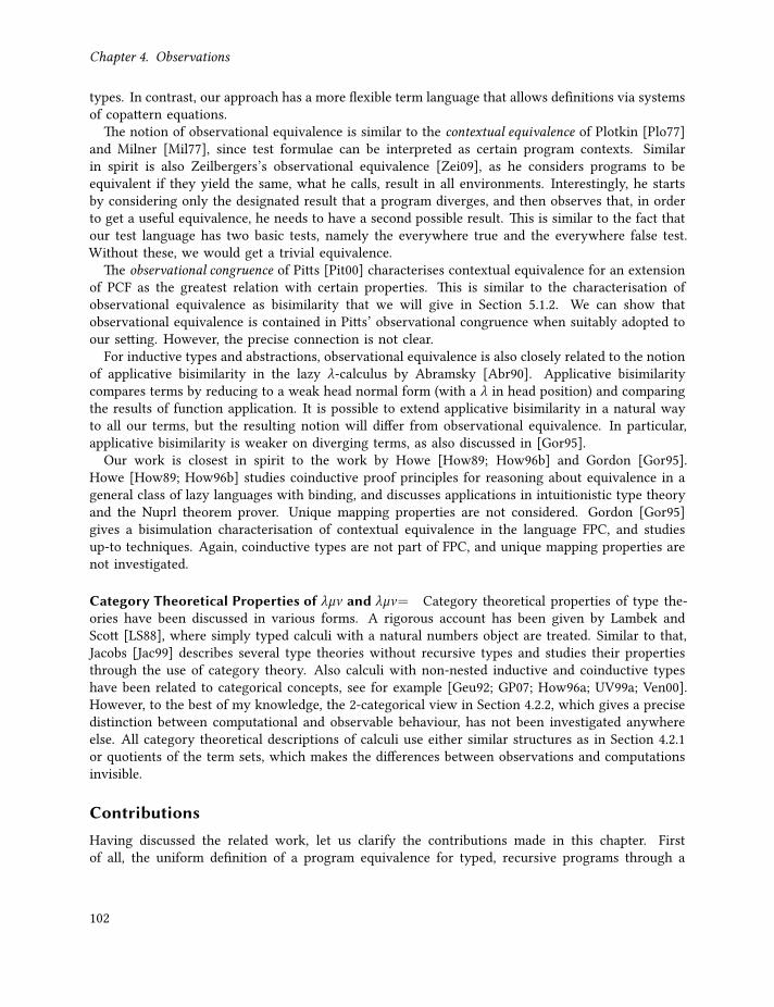
Chapter 4. Observations
types. In contrast, our approach has a more flexible term language that allows definitions via systemsof copattern equations.
The notion of observational equivalence is similar to the contextual equivalence of Plotkin [Plo77]and Milner [Mil77], since test formulae can be interpreted as certain program contexts. Similarin spirit is also Zeilbergers’s observational equivalence [Zei09], as he considers programs to beequivalent if they yield the same, what he calls, result in all environments. Interestingly, he startsby considering only the designated result that a program diverges, and then observes that, in orderto get a useful equivalence, he needs to have a second possible result. This is similar to the fact thatour test language has two basic tests, namely the everywhere true and the everywhere false test.Without these, we would get a trivial equivalence.
The observational congruence of Pitts [Pit00] characterises contextual equivalence for an extensionof PCF as the greatest relation with certain properties. This is similar to the characterisation ofobservational equivalence as bisimilarity that we will give in Section 5.1.2. We can show thatobservational equivalence is contained in Pitts’ observational congruence when suitably adopted toour setting. However, the precise connection is not clear.
For inductive types and abstractions, observational equivalence is also closely related to the notionof applicative bisimilarity in the lazy λ-calculus by Abramsky [Abr90]. Applicative bisimilaritycompares terms by reducing to a weak head normal form (with a λ in head position) and comparingthe results of function application. It is possible to extend applicative bisimilarity in a natural wayto all our terms, but the resulting notion will differ from observational equivalence. In particular,applicative bisimilarity is weaker on diverging terms, as also discussed in [Gor95].
Our work is closest in spirit to the work by Howe [How89; How96b] and Gordon [Gor95].Howe [How89; How96b] studies coinductive proof principles for reasoning about equivalence in ageneral class of lazy languages with binding, and discusses applications in intuitionistic type theoryand the Nuprl theorem prover. Unique mapping properties are not considered. Gordon [Gor95]gives a bisimulation characterisation of contextual equivalence in the language FPC, and studiesup-to techniques. Again, coinductive types are not part of FPC, and unique mapping properties arenot investigated.
Category Theoretical Properties of λµν and λµν= Category theoretical properties of type the-ories have been discussed in various forms. A rigorous account has been given by Lambek andScott [LS88], where simply typed calculi with a natural numbers object are treated. Similar to that,Jacobs [Jac99] describes several type theories without recursive types and studies their propertiesthrough the use of category theory. Also calculi with non-nested inductive and coinductive typeshave been related to categorical concepts, see for example [Geu92; GP07; How96a; UV99a; Ven00].However, to the best of my knowledge, the 2-categorical view in Section 4.2.2, which gives a precisedistinction between computational and observable behaviour, has not been investigated anywhereelse. All category theoretical descriptions of calculi use either similar structures as in Section 4.2.1or quotients of the term sets, which makes the differences between observations and computationsinvisible.
ContributionsHaving discussed the related work, let us clarify the contributions made in this chapter. Firstof all, the uniform definition of a program equivalence for typed, recursive programs through a
102

4.3. Conclusion and Related Work
testing logic has not been studied before. The testing logic builds thereby on the definition ofobservationally normalising terms, which are terms on which all observations are computable, thatis, any observation results in a strongly normalising term and least fixed point types only admitfinitely many consecutive unfolding steps. To my knowledge, such a notion has not been studied oncalculi that allow non-terminating programs, although the definition of observational normalisation isclosely related to the saturated sets semantics of types in strong normalisation proofs, see e.g. [AA99]and Chapter 7. More interesting, however, are the proof principles for observational equivalencethat we will establish in Chapter 5.
The second contribution in this chapter is the study of observational equivalence through the eyeof 2-categories. More specifically, we constructed 2-categories, whose objects are types, morphismsare equivalence classes of terms of λµν or λµν= under conversion, and 2-cells are given by theobservational equivalence of terms. This setup allowed us to characterise, for instance, producttypes as pseudo-products with strict choice. In particular, this means that on the product type thereare projections and one can pair morphisms. The crucial property of the paired morphism is thatits composition with the projections is strictly equal to the components, while the pairing itself isunique only up to isomorphism. Since strict equality corresponds to conversion and isomorphismscorrespond to observational equivalence, the notion of pseudo-product with strict choice capturesand distinguishes precisely the computational and observational behaviour of product types. Thus,the main contribution in Section 4.2 is this 2-category theoretical characterisation of computationaland observational behaviour of all types in the two calculi.
Future WorkThere is always room for improvements, but let us highlight one particular possibility for extendingthe 2-category view in Section 4.2.2. Recall that we defined a 2-category Cℓ≡s,obs(ON) that has onlyobservationally normalising terms of λµν= as morphisms. We can drop this restriction and obtain a2-category Cℓ≡s,obs(Λ
=) that has all λµν=-terms as morphisms. It seems that all proofs in Section 4.2.2can be adapted to this 2-category, so that also Cℓ≡s,obs(Λ
=) has pseudo-products, pseudo-coproductsetc. This raises of course the question what the relation is between Cℓ≡s,obs(Λ
=) and Cℓ≡s,obs(ON).Clearly, there is an inclusion 2-functor I : Cℓ≡s,obs(ON) → Cℓ
≡s,obs(Λ
=). Now note that Cℓ≡s,obs(ON)only consists of total functions, whereas Cℓ≡s,obs(Λ
=) also contains partial functions. Thus, we wouldexpect there to be a relation like the adjunction between the categories of sets with total functionsand sets with partial functions. In this classical case, a partial function f : X Y is sent to a totalfunction д : X + 1→ Y + 1, and the adjunction property expresses that a partial function f : X Ycorresponds to exactly one total function д : X → Y + 1:
X −− Y in Setpar
X −−→ Y + 1 in Set
However, the definition of д from f requires the law of excluded middle, because one definesд(x) = κ1(f (x)) if x ∈ dom(f ) and д(x) = κ2(∗) otherwise. Thus, it is not possible to write д as aprogram, since termination is not decidable in general.
Fortunately, an alternative to represent partial functions is offered by the so-called type of partialelements, which was first introduced by Capretta [Cap05]. For any type A ∈ Ty the type of partial
103

Chapter 4. Observations
A-elements is given in our type system by Aν B νX .A, where we obtain A by replacing every typevariable Y in A by X +Y . The idea is that every recursion step can now be captured through the typeAν . One needs to show that (−)ν can be extended to a functor Cℓ≡s,obs(Λ
=) → Cℓ≡s,obs(ON), whichis moreover right-adjoint to the inclusion. I conjecture that this can be done by instrumenting aprogram so that every computation step is recorded in Aν . For instance, recall from Example 4.1.22that the type 0 = µY .Y has no normalising inhabitant. However, we can define the term B = α Bof type 0 in λµν=. This term can be transformed into B : 0ν with 0ν = νX . µY .X + Y by putting
B.out = α (κ1 B).
The aim is thus to assign to each t with x : A ⊢ t : B an observationally normalising term twith x : A ⊢ t : Bν by means of such an instrumentation. Conversely, we can erase the partialityannotation from x : A ⊢ s : Bν by defining a term called extract of type Bν → B by induction onB. We can use extract to define a term s with x : A ⊢ s : B by putting s B extract s . These twoconstructions should give us then a correspondence
A −→ B in Cℓ≡s,obs(Λ=)
A −→ Bν in Cℓ≡s,obs(ON)
which is one-to-one up to observational equivalence. In other words, I conjecture that there is apseudo-adjunction as in the following diagram.
Cℓ≡s,obs(ON) Cℓ≡s,obs(Λ=)
I
(−)ν
⊣
The difficulty is the definition of the instrumented term t . I claim that t is computable, since itseems to be possible to define the instrumentation by induction on the term structure, cf. [Cap05,Sec. 4]. This in contrast to the classical approach, which requires us to decide termination. Butas the instrumentation is also a tedious process, I leave this for the future. One final note onthis instrumentation: One might be tempted to use directly the delay monad from [Cap05]. This,however, would not allow us to define the above advertised adjunction. For instance, if we use0ν = νX . 0 + X instead, then the only way to define B is by B.out = κ2 B, from which we cannotrecover a term that is observationally equivalent to B. This is the reason for the more complicatedinstrumentation, which allows us to preserve the observational behaviour of terms.
Following the program of Lambek and Scott [LS88], it would be natural to show that the classifying2-category of the calculus λµν is initial among all 2-categories that have the same closure properties,that is, which have all finite pseudo-products etc. This should not be a too difficult task, but it is leftopen for now. More intricate is to show that there is also a functor from the classifying 2-categoryof the observationally normalising terms in λµν= to the classifying 2-category of λµν . The difficultylies in the fact that systems of equations need to be reduced to iteration and coiteration. We alsoneed to leave this reduction open for now.
104
4.3. Conclusion and Related Work
Notes16 We could have called terms in ON persistently strongly normalising, in analogy with the similar
notion of the typed λ-calculus [BDS13, Sec. 17.2]. However, we favour the name observationallynormalising since it emphasises that terms in ON must be strongly normalising under all possibleobservations.
17 The fact that strong normalisation and the non-existence of infinite unfoldings on least fixed pointtypes do not coincide is actually an oversight in [BH16]. I would like to thank Andreas Abel forpointing this problem out to me, and preventing it therefore from slipping into my thesis.
18 See Example 2.4.3 for notation regarding families of sets.19 The interpretation in Definition 4.1.14 of tests on A as terms of type A→ Bool is similar to the notion
of observation from the λ-calculus [BDS13, Sec. 3.5]. However, there observations on function typesallow any term as argument, whereas we restrict to observationally normalising terms. This has theeffect that we identify terms of function type on the basis of their observational rather than theircomputational behaviour, see the discussion in the introduction of this chapter. This connection withthe λ-calculus is one reason for the name “observational equivalence”, another is that our notion isan instance of the coalgebraic notion of observable behaviour, as we will see in Section 5.1.
20 The notation E0A is used here because under the propositions-as-types interpretation, see Section 6.1, 0can be seen as the formula denoting falsum. Under this interpretation, the term E0A is the eliminationprinciple for 0.
21 Note that λD and д are similar to what Abramsky [Abr90] calls principal weak head normal forms.22 Usually, classifying categories are given for terms in arbitrary contexts. In that case, a classifiable
calculus would also have to satisfy weakening and exchange. However, the remaining developmentin this section does not require a general notion of classifying categories, and in fact is simpler inthe way it is presented. Note also that one could directly assume a calculus to be given in form ofa classifying category. But since the existence of such a category has to be proved in one way oranother, we prefer the given presentation, which allows us to give a general existence proof.
23 Note that the notion of classifying category that we use here is a simplification of the classifyingcategories in [Jac99].
24 Hayashi [Hay85] uses a slightly more complicated definition. The version that we use here isequivalent to the original one under the assumption of the distributivity law for products that weestablished in Lemma 4.2.6. This simplification was suggested to me by Andreas Abel.
25 It should be noted that pseudo-products, pseudo-coproducts, and pseudo-exponents with strict choiceare stronger than their weak counterparts. The reason is that we can alternatively define, for example,pseudo-products with strict choice as weak products, such that the pairing is unique up to a unique2-isomorphism.
26 In the proof of Lemma 4.2.13 we see that the coherence between vertical and horizontal compositionare automatically fulfilled, since in the classifying 2-categories there is at most one 2-cell between
105

Chapter 4. Observations
morphisms. In other words, the classifying 2-categories Cℓ≡s,obs(Λ) and Cℓ≡s,obs(ON) are order-enriched
(or even more specific: enriched over equivalence relations), cf. Definition 2.6.1. Such 2-categoriesare also called “locally posetal” by Lack [Lac10]. This property of the classifying 2-categories is goingto very useful in the following, as we always just have to prove that two terms are observationallyequivalent but we can save ourselves from proving any coherence conditions.
27 Note that πi h is a statement in the 2-category Cℓ≡s,obs(Λ). Recall that πi : A1 × A2 → Ai wasdefined, by abuse of notation, to be the term πi x . Thus πi h = (πi x)[h/x ] = πi h.
28 Definition 3.1.9 and Lemma 4.2.16 can both be given more generally for types T in which variablesXi occur in either negative position or in positive position. However, since we restrict attention tostrictly positive types, the current formulation suffices.
29 Sub-expressions of syntactic (Kripke-)polynomial functors are called ingredients by, for example,Kupke [Kup06].
106

CHAPTER 5
Inductive-Coinductive Reasoning
Here comes the argumentHere comes the argumentHere comes the argumentFolderol
— Fugazi, “Argument”, 2001.
In the last chapter we have constructed two languages that allow us to program with mixedinductive-coinductive types. Moreover, we have established a common notion of observationalequivalence on terms and, for the second language, singled out a class of observationally normalisingterms. The goal of this chapter is to establish methods of reasoning about inductive-coinductiveprograms, in particular methods for proving that programs are observationally equivalent. We willstudy three quite different proof methods, each having its own advantages and disadvantages, as wewill see.
In the remainder of this introduction we will discuss further the different proof methods thatwe advertised above. In Section 5.1, we obtain a proof technique for observational equivalencefrom a transition system that represents the observations that can be made on programs. Weshow that observational equivalence coincides with the canonical notion of bisimilarity that can beobtained by applying coalgebraic methods to the transition system. As such, the proof techniqueis readily usable but often requires the construction of annoyingly complicated relations. This canbe improved drastically through the use of up-to techniques, which we will demonstrate as well.As an illustration of the bisimulation proof method, we show that the substream relation, whichwe defined in Example 5.1.13, is transitive. Lastly, we also discuss the possibility of characterisingobservational normalisation as a coinductive predicate.
The proof techniques we have established up to here are fairly easy to prove correct and canbe used immediately. However, since they are cast in naive set theory, it becomes difficult toautomatically show, for instance, that a relation is a bisimulation because the description of thatrelation can be arbitrarily complex. Moreover, already the need to come up with an invariant thatdescribes a bisimulation is a huge burden and is unnecessary. In fact, the so-called bisimulation gameallows one to prove or disprove bisimilarity of processes interactively. The only problem with playsof a bisimulation game is that their correctness is difficult to ensure in general because of globalparity conditions that have to be checked. All three issues, automatic verification, upfront guessingand global correctness conditions, will be remedied by the syntactic proof systems for observationalequivalence in Section 5.2.
The syntactic proof system in Section 5.2 allows us to prove formulas of a first-order predicatelogic with an internal equality that models observational equivalence. Since the aim of the proofsystem is to allow for easy discovery of proof steps along the way, in contrast to having to guess abisimulation relation upfront, we opt for a recursive proof system. Such a proof system allows usto refer back to proof steps that we encountered before. To ensure that recursive references giverise to well-defined proofs, we use the so-called later modality [Nak00], which allows us to control
107

Chapter 5. Inductive-Coinductive Reasoning
where recursion steps can occur. In contrast to cyclic proof systems, our proof system allows proofsto be checked locally at every proof step. We describe this in detail in Section 5.2.
The two proof methods for observational equivalence that we discussed up to this point requiresome ingenuity in constructing proofs of program equivalences. In Section 5.3 we show that this isunavoidable, since observational equivalence is undecidable, as one would expect. More positively,we also establish there a fragment of the languages, on which observational equivalence is decidable.
Original Publication For the most part, the content of Section 5.1 has been presented in [BH16],but without the extensive example and the up-to technique for carrying out induction in a bisimu-lation proof in Section 5.1.3. In the same paper, also the results in Section 5.3 have been published.The logic FOL in Section 5.2 is, on the other hand, completely new. However, in [Bas18a] a generalapproach for constructing a logic for coinductive predicates, which is based on the later modality,from a logic given in form of a fibration is presented. This subsumes, in principle, the developmentin Section 5.2, see the discussion [Bas18a].
5.1. Program Properties as Coinductive PredicatesSince observational equivalence is defined in terms of tests, the only way to prove that two programsare equivalent is so far by induction on tests. In this section we develop a set-based proof techniquefor observational equivalence, which is simpler and more intuitively usable than induction on tests.This proof technique is centred around the idea that observations on programs give rise to a labelledtransition system on programs. We introduce this transition system in Section 5.1.1. Associated tosuch a transition system is the usual notion of bisimilarity. In Section 5.1.2 we show that observationalequivalence coincides with this notion of bisimilarity. This allows us to prove that programs areobservationally equivalent by establishing a bisimulation relation containing these terms, insteadof having to proceed by induction on tests. We demonstrate the use of this proof method on anextensive example in Section 5.1.3.
The description of observational equivalence as coinductive predicate gives us a powerful prooftechnique. However, this proof technique is also very tedious to use in its basic form, which leadsus to consider up-to techniques that can drastically reduce the complexity of equivalence proofs. Wegive in Section 5.1.2 several general up-to techniques, that can be used in any proof of observationalequivalence. In the example in Section 5.1.3, we also develop an up-to technique that allows us touse induction inside bisimulation proofs.
5.1.1. Terms as Transition SystemTowards coinductive proof principles for observational equivalence and observational normalisation,the first step is to establish a labelled transition system (LTS), in which the states are terms of λµν=.The labels in this transition system are the observations that are given by the modalities of thetesting logic in Definition 4.1.12. Given such a label, the successors of a term t are all those termsthat can be reached after making the observation given by that label.
The transition system on terms is defined by composing two relations. One relation, denoted by, represents the observations that can be made. For example, a possible observation on a term t
of type A× B is the first projection, which leads us to have a transition tπ1 π1 t in the transition
108

5.1. Program Properties as Coinductive Predicates
system. On an inductive type like A1 + A2 we can observe a constructor on terms of the formκi s for some term s of type Ai , in which case there is a transition κ1 s
κi s . Note that such atransition is only possible on terms in weak head normal form (Lemma 3.2.34). Thus, to avoid thatthe transition system gets stuck, we also need to take reductions into account. We can achieve thisby adding transitions to all terms that are reachable by reductions after making an observation ona term of coinductive type and before observing terms of inductive type. The transition relation weobtain from combining and reductions is denoted by .
The observation relation lA ⊆ Λ=(A) × Λ=(A) is given by the following rules. Note that the
relation is annotated with the type of the term on the left-hand side. This is necessary to decidewhen to make a reduction step in the definition of below.
t ∈ Λ=(A1 ×A2) i ∈ 1, 2
tπi
A1×A2t .pri
t ∈ Λ=(νX .XA)
tξ
νX .A t .out
t ∈ Λ=(A→ B) u ∈ ONA
t uA→B t u
t ∈ Λ=(Ai )
κi tκi
A1+A2t
t ∈ Λ=(A[µX .A/X ])
α t αµX .A t
The labelled transition relation lA ⊆ Λ=(A) × Λ=(A) is then defined by composing the labelled
observation relation with the reduction relation, as follows. Here ; denotes relation compositionand is the reflexive, transitive closure of the reduction relation −→, see Definition 3.2.14.30
lA=
; l
A if A is inductivel
A ; if A is coinductive
If the type A is clear from the context, we shall drop the subscript of this relation.Let us give some examples of transitions that can be taken in the above LTS. The first example
illustrates the need for reduction steps in between observations.
Example 5.1.1. Let A,B,C be types, and s and t be terms with s : A and t : C , so that we can form⟨κ1 s, t⟩ : (A+ B) ×C . There is now an observation step
⟨κ1 s, t⟩ π1 ⟨κ1 s, t⟩.pr1to a term of type A+ B. However, we cannot make any further observations, since the term on theright-hand side has no constructor in head position. So the observation relation gets stuck. Thisleads us to use the reduction relation to obtain
⟨κ1 s, t⟩.pr1 κ1 s,
from where we can again take an observation step
κ1 sκ1 s .
Thus the following sequence of steps is possible in the transition system.
⟨κ1 s, t⟩ π1 κ1 sκ1 s .
109

Chapter 5. Inductive-Coinductive Reasoning
Let us give some further and more concrete examples of possible transitions.
Example 5.1.2. We give several snapshots of the transition system, both on inductive and coinductivetypes. A full circle represents hereby a state of the transition system, whereas a dashed circlerepresents intermediate states.
1. The term ⟨ ⟩′ of type 1′ was defined in Example 3.2.7 so that ⟨ ⟩′.out ⟨ ⟩′. This leads to theloop displayed in the following diagram.
⟨ ⟩′ ⟨ ⟩′.outξ
It is noteworthy that we cannot extract any further information about ⟨ ⟩′, since ξ is theonly observation we can make on ⟨ ⟩′. In fact, this is what allowed us to show that 1′ is apseudo-terminal object in Theorem 4.2.14.
2. We display some transitions that start in the encoding 1 : Nat of 1. Recall that Nat = µX . 1+X ,and that the encoding was defined in Example 3.1.7 by 0 = α (κ1 ⟨ ⟩) and 1 = α (κ2 0).
1 κ2 0 0 κ1 ⟨ ⟩ ⟨ ⟩α κ2 α κ1
3. Of course, there are also terms in λµν= that have no outgoing transition because they do nothave a WHNF. For example, recall from Example 3.2.21 that we can define for any type A aterm ΩA = rlet f : Nat = · 7→ f in f , which has no normalising reductions. If we nowinstantiate this term for an inductive type, like for instance Nat, then ΩNat has no WHNF.This is to say that there is no term t : 1+ Nat with ΩNat α t . Thus there is no transitionoriginating from ΩNat in the LTS.
4. The final example is concerned with terms of coinductive types. Recall that we have definedin Example 3.2.9 a function term H : Natω → Natω → Natω . So for any observationallynormalising term u of type Natω there is a step H u H u possible. In particular, we canuse a term nats ∈ ONNatω that represents the stream (0, 1, 2, . . .) of natural numbers, seeExample 3.1.8. We show in the diagram in Figure 5.1 a part of the transition system, startingat H . It is important to note that we only display a fraction of the possible transitions, asthere is, for example, a transition originating from H for every term in u ∈ ONNatω and toevery term t with H u t .
We now give a description of the labelled transition relation (Λ=, ) as a coalgebra on terms.This will allow us to apply coalgebraic techniques to define bisimilarity on this labelled transitionsystem. An integral part of the transition relation on terms is that it is type-driven, whichin turn enforces that only terms of the same type can be related by a bisimulation relation. Weimplement this typing constraint in a coalgebra, which represents the transition system, by usingthe set family of terms indexed by their types. Thus, we consider Λ= as an element in SetTy, thecategory of set families indexed by types, see Example 2.4.3, and the transition system as a coalgebrafor a functor F : SetTy → SetTy. This functor describes the branching type of the transition system:for X ∈ SetTy and C ∈ Ty, F (X )C is the set that can be inspected by tests on type C , see the rules for
above. Formally F and the coalgebra representing the transition system are given as follows.
110

5.1. Program Properties as Coinductive Predicates
H nats H
H nats nats f 0 nats nats hd (f 0 nats nats)
tl (f 0 nats nats)H nats (tl nats) 0
1 H (tl nats) (tl2 nats)...
nats
· · · u nats
hd
tl
hd tl
Figure 5.1.: A few transitions in the LTS on terms originating at H
Definition 5.1.3. Let F : SetTy → SetTy be the functor given by
F (X )C =
1, C = 1⨿i ∈1,2 P(XAi ) + 1, C = A1 +A2
P(XA[µX .A/X ]) + 1, C = µX .A∏i ∈1,2 P(XAi ), C = A1 ×A2
P(XA[νX .A/X ]), C = νX .A
P(XB)ONA , C = A→ B
where P(−) is the covariant powerset functor, and for a set U , (−)U is the function space functor.F acts on morphisms in the obvious way. We define the coalgebra on terms δ : Λ= → F (Λ=) by
δ1(t) = ∗
δA1+A2(t) =
ιi (t ′ : Ai | t κi t
′), ∃t ′. t κi t′
∗, otherwise
δµX .A(t) =
t ′ : A | t α t ′, ∃t ′. t α t ′
∗, otherwise
δA1×A2(t)(i) = t ′ : Ai | πi t t ′
δνX .A(t) = t ′ : A | ξ t t ′δA→B(t)(u) = t ′ : C | t u t ′
Note that uniqueness of WHNFs, Lemma 3.2.33, ensures that δ is well-defined on sum types.31
111

Chapter 5. Inductive-Coinductive Reasoning
Of course, we would expect the transition system and the coalgebra δ to be equivalent. Toshow this, let us introduce another functor G : SetTy → SetTy. In the definition of G, we use theconstructors and projections as labels in the index of the corresponding coproducts and products.The reason for using F rather than G in the course of this chapter is that G is complicated. However,it simplifies the construction of a coalgebra from the transition system.
G(X )C =
⨿κi ∈κ1,κ2 P(XAi ) + 1, C = A1 +A2
1, C = 1⨿l ∈α P(XA[µX .A/X ]) + 1, C = µX .A∏πi ∈π1,π2 P(XAi ), C = A1 ×A2∏l ∈ξ P(XA[νX .A/X ]), C = νX .A∏u ∈ONA
P(XB), C = A→ B
Note that for fixed point types there is only one label, thus G(X )C is in these cases isomorphic toF (X )C . Similarly, we can rename the labels κi in the sum case to 1 and 2 and obtain thereby anisomorphism G(X )A1+A2
F (X )A1+A2. Analogously, G(X )C and F (X )C are also isomorphic for all
other types C . Since these isomorphisms are natural in X , we obtain an isomorphism F G. Wecan now associate a G-coalgebra (Λ=,d) with the rule-based transition system:
d : Λ= → G(Λ=)
dA(t) = ιℓ(t ′
t ℓA t ′
), A inductive and ∃t ′. t ℓ
A t ′
dA(t) = ∗, A inductive and ¬(∃t ′. t ℓA t ′)
dA(t)(ℓ) =t ′
t ℓA t ′
, A coinductive
Note that d is again well-defined on inductive types due to uniqueness of WHNFs. It is hopefullyclear that d is a G-coalgebraic representation of the relation . We now show that the F -coalgebraδ and the G-coalgebra d essentially define the same transition system.
Proposition 5.1.4. The transition systems defined by the F -coalgebra δ and by the G-coalgebra d areequivalent in the sense that the following diagram commutes.
F (Λ=)
Λ=
G(Λ=)
δ
d
Proof. Let f be the isomorphism G(Λ=) → F (Λ=). We proceed by case distinction in A ∈ Ty toshow that δA = fA dA.
112
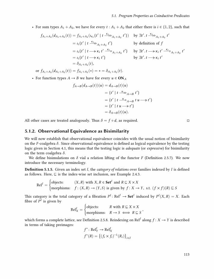
5.1. Program Properties as Coinductive Predicates
• For sum types A1 +A2, we have for every t : A1 +A2 that either there is i ∈ 1, 2, such that
fA1+A2(dA1+A2
(t)) = fA1+A2(ικi t ′ | t
κiA1+A2
t ′) by ∃t ′. t κiA1+A2
t ′
= ιi t ′ | t κiA1+A2
t ′ by definition of f
= ιi t ′ | t κi t′ κi
A1+A2t ′ by ∃t ′. t κi t
′ κiA1+A2
t ′
= ιi t ′ | t κi t′ by ∃t ′. t κi t
′
= δA1+A2(t),
or fA1+A2(dA1+A2
(t)) = fA1+A2(∗) = ∗ = δA1+A2
(t).
• For function types A→ B we have for every u ∈ ONA
fA→B(dA→B(t))(u) = dA→B(t)(u)
= t ′ | t uA→B t ′
= t ′ | t uA→B t u t ′
= t ′ | t u t ′= δA→B(t)(u).
All other cases are treated analogously. Thus δ = f d , as required.
5.1.2. Observational Equivalence as BisimilarityWe will now establish that observational equivalence coincides with the usual notion of bisimilarityon the F -coalgebra δ . Since observational equivalence is defined as logical equivalence by the testinglogic given in Section 4.1, this means that the testing logic is adequate (or expressive) for bisimilarityon the term coalgebra δ .
We define bisimulations on δ vial a relation lifting of the functor F (Definition 2.5.7). We nowintroduce the necessary terminology.Definition 5.1.5. Given an index set I , the category of relations over families indexed by I is definedas follows. Here, ⊑ is the index-wise set inclusion, see Example 2.4.3.
RelI =objects: (X ,R) with X ,R ∈ SetI and R ⊑ X × Xmorphisms: f : (X ,R)→ (Y , S) is given by f : X → Y , s.t. (f × f )(R) ⊑ S
This category is the total category of a fibration P I : RelI → SetI induced by P I (X ,R) = X . Eachfibre of P I is given by
RelIX =
objects: R with R ⊑ X × Xmorphisms: R → S ⇐⇒ R ⊑ S
,
which forms a complete lattice, see Definition 2.5.8. Reindexing on RelI along f : X → Y is describedin terms of taking preimages:
f ∗ : RelIY → RelIXf ∗(R) =
(fi × fi )
−1(Ri )i ∈I
113

Chapter 5. Inductive-Coinductive Reasoning
We will omit I in the superscripts of Rel and P , if it is understood from the context.
Recall from Definition 2.5.7 that a lifting H to RelI of a functor L : SetI → SetI restricts for eachX ∈ SetI to a functor HX : RelIX → RelILX on fibres, and that we can model for a given coalgebrac : X → LX relational properties of c as final coalgebras for the functor Hc : RelIX → RelIX , where
Hc B c∗ HX .
In particular, it is well-known that bisimulations for δ : Λ= → F (Λ=) are exactly the post-fixedpoints of F δ , where F is the canonical relation lifting of F , see [Sta11].
Definition 5.1.6. The canonical relation lifting F : RelTy → RelTy of F is given by
F (X ,R) = (FX , ⟨F (π1), F (π2)⟩(FR)).
Let Φ: RelTyΛ= → RelTyΛ= be the monotone map
Φ B F δ = δ ∗ FX .
An observational bisimulation is a Φ-invariant (or F -bisimulation on δ ), see Definition 2.5.7, that is,a relation R ∈ RelTyΛ= on terms, such that
R ⊑ Φ(R).
Notation 5.1.7. In the remainder of this chapter, we will only use type-indexed relations. So tokeep the notation simple, we omit the superscript in RelTy and just write Rel.
Let us describe the canonical lifting of F and the monotone operator Φ, more concretely. Suppose,we are given R ∈ RelΛ= . Then for all (U1,U2) ∈ F (Λ=)A × F (Λ=)A, we have
(U1,U2) ∈ F (R)A ⇐⇒ ∃U ∈ F (R)A.U1 = (Fπ1)A(U ) and U2 = (Fπ2)A(U ).
Thus we haveΦ(R)A = (t1, t2) ∈ Λ=(A)2 | (δA(t1),δA(t2)) ∈ F (R)A.
Let us now give an explicit description of the properties that a relation has to fulfil in order to bean observational bisimulation. The easiest case to spell out the requirements on an observationalbisimulation is if we do not have to take explicit reduction steps into account. This is captured inthe following lemma, for which we recall that ≡ denotes the convertibility relation, Definition 3.2.14.
Lemma 5.1.8. Let R ∈ RelΛ= and assume that R is ≡-closed, that is, for all (s, t) ∈ RA, s ≡ u and t ≡ v ,the pair (u,v) is also in RA. Then R is an observational bisimulation if and only if the following conditionsare fulfilled.
• If (s, t) ∈ RA1+A2, then either neither of s and t has a WHNF, or there is an i ∈ 1, 2 with s ≡ κi s ′,
t ≡ κi t ′ and (s ′, t ′) ∈ RAi .
• If (s, t) ∈ RµX .A, then either neither of s and t has a WHNF, or s ≡ α s ′, t ≡ α t ′ and (s ′, t ′) ∈RA[µX .A/X ].
114

5.1. Program Properties as Coinductive Predicates
• If (s, t) ∈ RA1×A2, then (s .pr1, t .pr1) ∈ RA1
and (s .pr2, t .pr2) ∈ RA2.
• If (s, t) ∈ RA→B , then for all u ∈ ONA we must have (s u, t u) ∈ RB .
• If (s, t) ∈ RνX .A, then (s .out, t .out) ∈ RA[νX .A/X ].
Proof. Let R ∈ RelΛ= be ≡-closed. We need to show that R ⊑ Φ(R) if and only if the above conditionshold. So let A be a type and (s, t) ∈ RA. That (s, t) ∈ Φ(R)A is equivalent to the correspondingcondition for each type A ∈ Ty is shown by case distinction on A. We only demonstrate theseequivalences on function types and least fixed point types, since the other cases are dealt withanalogously.
• Suppose that (s, t) ∈ Φ(R)A→B . We need to show that this is equivalent to saying that∀u ∈ ONA. (s u, t u) ∈ RB . First, we can rewrite the condition (s, t) ∈ Φ(R)A→B to clausesthat are familiar from labelled transition systems without using the fact that R is ≡-closed:
(s, t) ∈ Φ(R)A→B
⇐⇒ (δA→B(s),δA→B(t)) ∈ F (R)A→B
⇐⇒ ∃U ∈ P(RB)ONA . δA→B(s) = (Fπ1)(U ) ∧ δA→B(t) = (Fπ2)(U )
⇐⇒ ∃U ∈ P(RB)ONA . ∀u ∈ ONA.
∀s ′ ∈ δA→B(s)(u). ∃t ′. (s ′, t ′) ∈ U (u) ∧ ∀(s ′, t ′) ∈ U (u). s ′ ∈ δA→B(s)(u)
∧ ∀t ′ ∈ δA→B(t)(u). ∃s ′. (s ′, t ′) ∈ U (u) ∧ ∀(s ′, t ′) ∈ U (u). t ′ ∈ δA→B(t)(u)
⇐⇒ ∀u ∈ ONA. ∀s ′ ∈ δA→B(s)(u). ∃t ′ ∈ δA→B(t)(u). (s′, t ′) ∈ RB
∧∀t ′ ∈ δA→B(t)(u). ∃s ′ ∈ δA→B(s)(u). (s′, t ′) ∈ RB
⇐⇒ ∀u ∈ ONA. ∀s ′. (s u s ′) =⇒ (∃t ′. t u t ′ ∧ (s ′, t ′) ∈ RB)∧∀t ′. (t u t ′) =⇒ (∃s ′. s u s ′ ∧ (s ′, t ′) ∈ RB)
Since R is closed under conversions, we obtain then the desired property:
(s, t) ∈ Φ(R)A→B
⇐⇒ ∀u ∈ ONA. ∀s ′. (s u s ′) =⇒ (∃t ′. t u t ′ ∧ (s ′, t ′) ∈ RB)∧∀t ′. (t u t ′) =⇒ (∃s ′. s u s ′ ∧ (s ′, t ′) ∈ RB)
see above
⇐⇒ ∀u ∈ ONA. ∀s ′. (s u s ′) =⇒ (s ′, t u) ∈ RB∧∀t ′. (t u t ′) =⇒ (s u, t ′) ∈ RB
R ≡-closed
⇐⇒ ∀u ∈ ONA. (s u, t u) ∈ RB ∧ (s u, t u) ∈ RB R ≡-closed⇐⇒ ∀u ∈ ONA. (s u, t u) ∈ RB .
Therefore, we have that (s, t) ∈ Φ(R)A→B ⇐⇒ ∀u ∈ ONA. (s u, t u) ∈ RB , and thus, onfunction types, R ⊆ Φ(R)A→B is equivalent to
∀(s, t). (s, t) ∈ R =⇒ ∀u ∈ ONA. (s u, t u) ∈ RB .
115
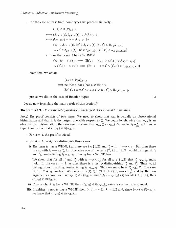
Chapter 5. Inductive-Coinductive Reasoning
• For the case of least fixed point types we proceed similarly:
(s, t) ∈ Φ(R)µX .A
⇐⇒ (δµX .A(s),δµX .A(t)) ∈ F (R)µX .A
⇐⇒ δµX .A(s) = ∗ = δµX .A(t)∨(∀s ′ ∈ δµX .A(s). ∃t ′ ∈ δµX .A(t). (s′, t ′) ∈ RA[µX .A/X ]
∧ ∀t ′ ∈ δµX .A(t). ∃s ′ ∈ δµX .A(s). (s′, t ′) ∈ RA[µX .A/X ]
)⇐⇒ neither s nor t has a WHNF ∨(∀s ′. (s α s ′) =⇒ (∃t ′. t α t ′ ∧ (s ′, t ′) ∈ RA[µX .A/X ])
∧ ∀t ′. (t α t ′) =⇒ (∃s ′. s α s ′ ∧ (s ′, t ′) ∈ RA[µX .A/X ]))
From this, we obtain
(s, t) ∈ Φ(R)A→B
⇐⇒ neither s nor t has a WHNF ∨∃s ′, t ′. s ≡ α s ′ ∧ t ≡ α t ′ ∧ (s ′, t ′) ∈ RA[µX .A/X ],
just as we did in the case of function types.
Let us now formulate the main result of this section.32
Theorem 5.1.9. Observational equivalence is the largest observational bisimulation.
Proof. The proof consists of two steps: We need to show that ≡obs is actually an observationalbisimulation and that it is the largest one with respect to ⊑. We begin by showing that ≡obs is anobservational bisimulation, thus we need to show that ≡obs ⊑ Φ(≡obs). So we let t1 ≡Aobs t2 for sometype A and show that (t1, t2) ∈ Φ(≡obs)A.
• For A = 1, the proof is trivial.
• For A = A1 +A2, we distinguish three cases.i) The term t1 has a WHNF, i.e., there are i ∈ 1, 2 and t ′1 with t1 κi t
′1. But then there
is a t ′2 with t2 κi t′2, for otherwise one of the tests [⊤,⊥] or [⊥,⊤] would distinguish t1
and t2, contradicting t1 ≡obs t2. Thus t2 has a WHNF, too.We show that for all t ′1 and t ′2 with tk κi t
′k for all k ∈ 1, 2 that t ′1 ≡obs t ′2 must
hold. In the case i = 1, assume there is a test ϕ distinguishing t ′1 and t ′2. Then [ϕ,⊥]distinguishes t1 and t2, contradicting t1 ≡obs t2. Thus we must have t ′1 ≡obs t ′2. The caseof i = 2 is symmetric. We put U =
(t ′1, t
′2)
∀k ∈ 1, 2. tk κi t′k
and by the two
arguments above, we have ιi (U ) ∈ F (≡obs)A and δ(tk ) = ιi (πk (X )) for all k ∈ 1, 2, thus(t1, t2) ∈ Φ(≡obs)A.
ii) Conversely, if t2 has a WHNF, then (t1, t2) ∈ Φ(≡obs)A using a symmetric argument.iii) If neither t1 nor t2 has a WHNF, then δ(tk ) = ∗ for k = 1, 2 and, since (∗, ∗) ∈ F (≡obs)A,
we have that (t1, t2) ∈ Φ(≡obs)A.
116

5.1. Program Properties as Coinductive Predicates
• The case A = µX . B is proved analogously.
• If A = B → C , we have for each u ∈ ONB and t ′k with tk u t ′k and k ∈ 1, 2 thatt ′1 ≡obs t ′2. Assume that t ′1 and t ′2 could be distinguished by a test ϕ, then the test [u]ϕ woulddistinguish t1 and t2, which contradicts t1 ≡obs t2. Thus, t ′1 ≡obs t ′2 for all such t ′1 and t ′2.Now let X (u) = (t ′1, t ′2) | ∀k ∈ 1, 2. tk u t ′k . By the above discussion, X ∈ F (≡obs)A,and by definition, also πk (X (u)) = δ(tk )(u) for all 1, 2 and for all u ∈ ONB , hence(t1, t2) ∈ Φ(≡obs)A.
• The cases for products and greatest fixed point types can be proved analogously.
Having proved that ≡obs is an observational bisimulation, it remains to prove that ≡obs is the largestsuch bisimulation. So let R ∈ RelΛ= be such that R ⊑ Φ(R). We show that R ⊑ ≡obs by showing thatfor all A ∈ Ty, all (t1, t2) ∈ RA and all ϕ : A that t1 ⊨ ϕ ⇔ t2 ⊨ ϕ holds. The proof is by inductionon ϕ. The base case for the trivial tests ⊤ and ⊥ is immediate. We prove the induction step by casedistinction in A.
• If A = A1 + A2, then, since R is a bisimulation, either δ(t1) = δ(t2) = ∗ or there is ani ∈ 1, 2 such that
∀t ′1. (t1 κi t′1) =⇒ (∃t ′2. t2 κi t
′2 ∧ (t ′1, t
′2) ∈ RAi ) (5.1)
∀t ′2. (t2 κi t′2) =⇒ (∃t ′1. t1 κi t
′1 ∧ (t ′1, t
′2) ∈ RAi ) (5.2)
We use this to show that t1 and t2 satisfy ϕ simultaneously. If there is k ∈ 1, 2 such thatδ(tk ) = ∗, then tk does not have a WHNF and both t1 and t2 do not satisfy ϕ. Otherwise, weuse that the test ϕ must be of the form [ψ1,ψ2] with ψi :↓ Bi . By definition, t1 ⊨ ϕ ⇔ t ′1 ⊨ ψifor t1 ≡ κi t ′1. The existence of t ′1 with t1 ≡ κi t ′1 implies that there is a t ′′1 with t1 κi t
′′1 .
By (5.1), there is a t ′2 with t2 κi t′2 and (t ′′1 , t
′2) ∈ RAi . Finally, by the induction hypothesis,
t ′1 and t ′2 simultaneously satisfy ψi , hence t2 ⊨ ϕ. Using (5.2), we prove analogously that t2 ⊨ ϕimplies t1 ⊨ ϕ.
• We proceed analogously for least fixed point types.
• If A = B → C , then the assumption RA ⊆ Φ(R)A says that for all u ∈ ONB
∀t ′1. (t1 u t ′1) =⇒ (∃t ′2. t2 u t ′2 ∧ (t ′1, t′2) ∈ RC ) (5.3)
∀t ′2. (t2 u t ′2) =⇒ (∃t ′1. t1 u t ′1 ∧ (t ′1, t′2) ∈ RC ) (5.4)
This allows us to show that t1 ⊨ ϕ ⇔ t2 ⊨ ϕ. The test ϕ must be of the form [u]ψ for someu ∈ ONB and ψ :↓C . By (5.3), there is a t2 u t ′2 with (t1 u, t
′2) ∈ RC , which implies by
induction that t1 u and t ′2 simultaneously satisfy ψ . Moreover, t2 u t ′2 implies that t2 u andt ′2 simultaneously satisfy ψ . Hence t1 u ⊨ ψ ⇒ t2 u ⊨ ψ and thus t1 ⊨ ϕ ⇒ t2 ⊨ ϕ. Analogously,we prove t2 ⊨ ϕ ⇒ t1 ⊨ ϕ by (5.4), thus t1 and t2 simultaneously satisfy ϕ.
• The case for products and greatest fixed points is proved analogously.
Thus ≡obs is the largest observational bisimulation, hence it is final for Φ.
117
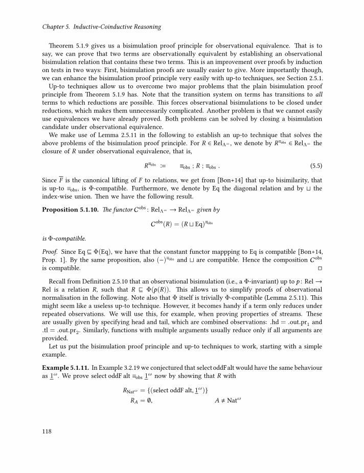
Chapter 5. Inductive-Coinductive Reasoning
Theorem 5.1.9 gives us a bisimulation proof principle for observational equivalence. That is tosay, we can prove that two terms are observationally equivalent by establishing an observationalbisimulation relation that contains these two terms. This is an improvement over proofs by inductionon tests in two ways: First, bisimulation proofs are usually easier to give. More importantly though,we can enhance the bisimulation proof principle very easily with up-to techniques, see Section 2.5.1.
Up-to techniques allow us to overcome two major problems that the plain bisimulation proofprinciple from Theorem 5.1.9 has. Note that the transition system on terms has transitions to allterms to which reductions are possible. This forces observational bisimulations to be closed underreductions, which makes them unnecessarily complicated. Another problem is that we cannot easilyuse equivalences we have already proved. Both problems can be solved by closing a bisimulationcandidate under observational equivalence.
We make use of Lemma 2.5.11 in the following to establish an up-to technique that solves theabove problems of the bisimulation proof principle. For R ∈ RelΛ= , we denote by R≡obs ∈ RelΛ= theclosure of R under observational equivalence, that is,
R≡obs B ≡obs ; R ; ≡obs . (5.5)
Since F is the canonical lifting of F to relations, we get from [Bon+14] that up-to bisimilarity, thatis up-to ≡obs, is Φ-compatible. Furthermore, we denote by Eq the diagonal relation and by ⊔ theindex-wise union. Then we have the following result.
Proposition 5.1.10. The functor Cobs : RelΛ= → RelΛ= given by
Cobs(R) = (R ⊔ Eq)≡obs
is Φ-compatible.
Proof. Since Eq ⊑ Φ(Eq), we have that the constant functor mappping to Eq is compatible [Bon+14,Prop. 1]. By the same proposition, also (−)≡obs and ⊔ are compatible. Hence the composition Cobs
is compatible.
Recall from Definition 2.5.10 that an observational bisimulation (i.e., a Φ-invariant) up to p : Rel→Rel is a relation R, such that R ⊑ Φ(p(R)). This allows us to simplify proofs of observationalnormalisation in the following. Note also that Φ itself is trivially Φ-compatible (Lemma 2.5.11). Thismight seem like a useless up-to technique. However, it becomes handy if a term only reduces underrepeated observations. We will use this, for example, when proving properties of streams. Theseare usually given by specifying head and tail, which are combined observations: .hd = .out.pr1 and.tl = .out.pr2. Similarly, functions with multiple arguments usually reduce only if all arguments areprovided.
Let us put the bisimulation proof principle and up-to techniques to work, starting with a simpleexample.
Example 5.1.11. In Example 3.2.19 we conjectured that selectoddFalt would have the same behaviouras 1ω . We prove select oddF alt ≡obs 1ω now by showing that R with
RNatω = (select oddF alt, 1ω)RA = ∅, A , Natω
118

5.1. Program Properties as Coinductive Predicates
is an observational bisimulation up to Φ Cobs. Recall from Example 3.2.19 that
(select oddF alt).hd ≡ 1
(select oddF alt).tl ≡ select oddF altand
(1ω).hd ≡ 1
(1ω).tl ≡ 1ω
Since (1, 1) ∈ Cobs(R)Nat and (select oddF alt, 1ω) ∈ RωNat ⊆ Cobs(R)Natω , we have
((select oddF alt).out, (1ω).out) ∈ Φ(Cobs(R))Nat×Natω
and hence(select oddF alt, 1ω) ∈ Φ(Φ(Cobs(R)))Natω .
So R is indeed an observational bisimulation up to Φ Cobs.
Example 5.1.11 shows that it requires some ingenuity to combine up-to techniques in the correctorder for a proof to go through. So it would be useful if there was a way to introduce up-totechniques in a proof whenever necessary without the need to correctly specify the order of usebeforehand. Fortunately, this can be achieved by using the companion of Φ that we introducedin Definition 2.5.12. For instance, the companion allows us to close a relation backwards underobservations, as the following lemma shows.
Lemma 5.1.12. Let R ∈ RelΛ= . The companion γΦ of Φ, see Definition 2.5.12, fulfils the followingbackwards closure conditions.
• If for all u ∈ ONA we have (s u, t u) ∈ γΦ(R)B , then (s, t) ∈ γΦ(R)A→B .
• If for all i ∈ 1, 2 we have (πi s,πi t) ∈ γΦ(R)Ai , then (s, t) ∈ γΦ(R)A1×A2.
• If (s .out, t .out) ∈ γΦ(R)A[νX .A/X ], then (s, t) ∈ γΦ(R)νX .A.
Proof. We only prove the case for functions, the other cases are analogous. Recall from Lemma 5.1.8that ∀u ∈ ONA. (s u, t u) ∈ γΦ(R)B is equivalent to (s, t) ∈ Φ(γΦ(R))A→B . Since Φ is compatible, wehave Φ(γΦ(R)) ⊑ γΦ(R). Thus, (s, t) ∈ γΦ(R)A→B follows.
5.1.3. An Extensive Example: Transitivity of the Substream RelationWe will now study an elaborate example that demonstrates the use of the bisimulation proof method,up-to techniques and the companion. In this example, we show that the following substream relationis transitive.
Example 5.1.13. Recall that a stream selector was given as element of the type F , where F =νX . µX .X + Y . Let s, t : Natω be stream terms in We say that s is substream of t , written s ≤ t , ifthere is a selector x ∈ ONF such that select x s ≡obs t . Symbolically, we define
s ≤ t B ∃x ∈ ONF . s ≡obs select x t .
To prove transitivity, we observe that if r ≤ s by x1 and s ≤ t by x2, then
t ≡obs select x2 s ≡obs select x2 (select x1 r). (5.6)
119

Chapter 5. Inductive-Coinductive Reasoning
We thus expect to be able to relate r and t directly by some form of composition of selectors. Indeed,we can compose selectors in λµν= as follows, where Fµ = µX .X + F .
comp : F → F → F
(comp x y).out = compµ (x .out) (y.out)compµ : Fµ → Fµ → Fµ
compµ (pres x) (pres y) = pres (comp x y)compµ (pres x) (dropv) = drop (compµ (x .out)v)compµ (drop u)v = drop (compµ u v)
Note that comp is defined coinductively, whereas compµ is defined first by iteration on the firstargument, and then in the base case of the first argument by iteration on the second argument. Letus introduce some more visually appealing notation for the composition of selectors:
y • x B comp x y y •µ x B compµ x y.
If we can show thatselect (y • x) ≡obs select y select x , (5.7)
then we can continue the chain of equations in (5.6) with
t ≡obs select x2 (select x1 r) ≡obs select (x2 • x1) r .
Hence, the selector that witnesses r ≤ t is given by composing the selectors that witness r ≤ s ands ≤ t , respectively.
The rest of this subsection is devoted to proving (5.7). A first step towards this is to prove aninduction principle that allows us to prove observational equivalence of maps out of Fµ . This requiresthe characterisation of the elements in Fµ , which is the content of the following lemma.
Lemma 5.1.14. For all u ∈ ONFµ there are n ∈ N and x ∈ ONF , such that u ≡ dropn (pres x).
Proof. Since u ∈ ONFµ ⊆ SNFµ , by Lemma 3.2.34 there is an i ∈ 1, 2 and an observationallynormalising u ′ with u α (κi u
′). If i = 1, then α (κi u′) = pres u ′, thus u ≡ drop0 (pres u ′).
Hence, the claim holds with x = u ′. Otherwise, if i = 2, then α (κi u′) = drop u ′. As u ′ is a finite
term and strongly normalising, we get by induction on the reduction steps towards a normal formof u ′ that there are x ∈ ONF and k ∈ N, such that u ′ ≡ dropk (pres x). Hence, the claim holds inthis case with n = k + 1, that is, we have u ≡ dropk+1 (pres x).
Given the characterisation of elements in Fµ , we now construct an operator that closes a relationunder the application to arguments in Fµ . The idea is that whenever there are terms s and t relatedby RFµ→A, then we would like to extend R, such that s u and t u are related for all u ∈ Fµ . In general,this is not sound as an up-to technique. However, if we assume that s u and t u are related by RA inthe base case where u ≡ pres x for some x : F , and that R is closed under induction steps, then wecan safely build a closure of R that contains all pairs (s u, t u). This closure is given in the followingdefinition.
120

5.1. Program Properties as Coinductive Predicates
Definition 5.1.15. We define H : [RelΛ= ,RelΛ= ] → [RelΛ= ,RelΛ= ], where [RelΛ= ,RelΛ= ] is the setof monotone functions on RelΛ= , as follows by using the closure under convertibility (−)≡.
H(T )(R)A = (s u, t u) |(s, t) ∈ RFµ→A ∧ u ∈ ONFµ ∧ x ∈ ONF ∧ u ≡ pres x∧ (s (pres x), t (pres x)) ∈ RA
∪ (s u, t u) |(s, t), (s ′, t ′) ∈ RFµ→A ∧ u,u ′ ∈ ONFµ
∧ s (drop u ′) ≡ s ′ u ′ ∧ t (drop u ′) ≡ t ′ u ′
∧ (s ′ ′, t ′u ′) ∈ T (R)≡A
The Fµ -closure is the least fixed point µH : RelΛ= → RelΛ= of H .
We show that the inductive closure µH is sound as an up-to technique, by proving that it iscontained in the companion of Φ. Thus, we can use µH in all proofs of bisimilarity up to γΦ.
Lemma 5.1.16. µH is contained in the companion of Φ: µH ⊑ γΦ.
Proof. To show that µH ⊑ γΦ, we need to prove that µH(R)A ⊆ γΦ(R)A for all R ∈ RelΛ= andA ∈ Ty. Since µH is a fixed point of H , it suffices to prove H(µH)(R)A ⊆ γΦ(R)A. So let (s u, t u) ∈H(µH)(R)A for some (s, t) ∈ RFµ→A by one of the clauses of H . We proceed by induction on n foru ≡ dropn (pres x), see Lemma 5.1.14.
• If n = 0, then the first case of H applies and we have (s (pres x), t (pres x)) ∈ RA. Thus also(s (pres x), t (pres x)) ∈ γΦ(R)A. Since Cobs is compatible by Proposition 5.1.10, it is containedin the companion, which means that the companion is ≡-closed. Thus, (s u, t u) ∈ γΦ(R)A.
• If n = k +1, then by the second case of H we get (s ′, t ′) ∈ RFµ→A, such that s (dropu ′) ≡ s ′u ′,t (drop u ′) ≡ t ′ u ′ and (s ′ u ′, t ′ u ′) ∈ µH(R)A, where u ′ = dropk (pres x). By the inductionhypothesis for k , we thus obtain (s ′ u ′, t ′ u ′) ∈ γΦ(R)A. Appealing again to the ≡-closure ofγΦ, we thus have (s u, t u) ∈ γΦ(R)A, as required.
Hence, µH(R)A = H(µH)(R)A ⊆ γΦ(R)A for all R and A, and so µH ⊑ γΦ.
It is fairly hard to use the definition of µH directly in a bisimilarity proof because it is not clearwhich conditions R needs to satisfy in order for µH(R)A to contain (s u, t u) for all (s, t) ∈ RFµ→Aand u ∈ ONFµ . In the lemma below, we establish such conditions on a given relation R and theterms related by RFµ→A, which leads to a proof principle that allows us to easily apply µH . Theseconditions essentially require that RA relates terms in the base case of Fµ and that R is closed undercomputations in the induction step.33
Lemma 5.1.17. Let R ∈ RelΛ= and A ∈ Ty. Suppose that for all (s, t) ∈ RFµ→A and all monotoneT : RelΛ= → RelΛ= the following conditions hold:
i) ∀x ∈ ONF . (s (pres x), t (pres x)) ∈ RA and
ii) ∀u ∈ ONFµ . ∃(s ′, t ′) ∈ RFµ→A. (s′ u, t ′ u) ∈ T (R)A =⇒ (s (drop u), t (drop u)) ∈ T (R)≡A
Then for all u ∈ ONFµ and all (s, t) ∈ RFµ→A we have (s u, t u) ∈ µH(R)A.
121

Chapter 5. Inductive-Coinductive Reasoning
Proof. Let R andA be given as required by the lemma. Suppose now that u ∈ ONFµ . By Lemma 5.1.14,there is an n ∈ N and an x ∈ ONF , such that u ≡ dropn (pres x). We proceed by induction on n toprove for all (s, t) ∈ RFµ→A that (s u, t u) ∈ µH(R)A.
• If n = 0, then u ≡ pres x . Condition i) gives us that (s (pres x), t (pres x)) ∈ RA. By definitionof H (Definition 5.1.15), we thus have (s u, t u) ∈ H(µH)(R)A, and by µH being a fixed pointof H hence (s u, t u) ∈ µH(R)A.
• If n = k +1, then u ≡ dropu ′ for u ′ = dropk (presx). From condition ii), we get with T = µHa pair (s ′, t ′) ∈ RFµ→A, such that, (s ′u ′, t ′u ′) ∈ µH(R)A would imply (s (dropu ′), t (dropu ′)) ∈µH(R)≡A. Since by induction we have for any (s ′, t ′) ∈ RFµ→A that (s ′ u ′, t ′ u ′) ∈ µH(R)A, wethus obtain (s (drop u ′), t (drop u ′)) ∈ µH(R)≡A. By definition of H , this implies (s u, t u) ∈H(µH)(R)A. Hence, again by µH being a fixed point, it follows that (s u, t u) ∈ µH(R)A.
This induction on n shows for all (s, t) ∈ RFµ→A that (s u, t u) ∈ µH(R)A, as required.
The induction principle that we devised in Lemma 5.1.17 is readily usable, if we want to prove thattwo functions with one argument in Fµ are observationally equivalent. However, (5.7) requires usto prove an equivalence between functions with two arguments in Fµ , see Proposition 5.1.19 belowfor details. We could apply Lemma 5.1.17 twice in this situation, but note that compµ does not doany further pattern matching on the second argument in the last case of its definition. Hence, weonly need to distinguish three cases: both arguments are given by the pres-constructor; the first isa pres- and the second drop-constructor; and the first is given by the drop-constructor, while thesecond argument is arbitrary. The following lemma applies Lemma 5.1.17 twice to obtain a mutualinduction principle that captures exactly this situation.34
Lemma 5.1.18. Let R ∈ RelΛ= and A ∈ Ty. Suppose that for all (s, t) ∈ RFµ→Fµ→A and all monotoneT : RelΛ= → RelΛ= the following conditions hold:
i) ∀x ,y ∈ ONF . (s (pres x) (pres y), t (pres x) (pres y)) ∈ RA,
ii) ∀v ∈ ONFµ . ∃(s ′, t ′) ∈ RFµ→Fµ→A.
(∀u ∈ ONFµ . (s′ u v, t ′ u v) ∈ T (R)A)
=⇒ ∀x ∈ ONF . (s (pres x) (dropv), t (pres x) (dropv)) ∈ T (R)≡Aiii) ∀u,v ∈ ONFµ . ∃(s ′, t ′) ∈ RFµ→Fµ→A.
(s ′ u v, t ′ u v) ∈ T (R)A =⇒ (s (drop u)v, t (drop u)v) ∈ T (R)≡AThen for all (s, t) ∈ RFµ→Fµ→A and all u,v ∈ ONFµ we have (s u v, t u v) ∈ γΦ(R)A.Proof. The proof proceeds by applying Lemma 5.1.17 to the second argument to show that we have(λu . s u v, λu . t u v) ∈ µH(γΦ(R))Fµ→A for all v ∈ ONFµ . Two cases arise from this: First, we needto prove for all y ∈ ONF that (λu . s u (pres y), λu . t u (pres y)) ∈ γΦ(R)Fµ→A, and, second, that forall operators T and all v ′ ∈ ONFµ also (λu . s u (drop v ′), λu . t u (drop v ′)) ∈ T (γΦ(R))Fµ→A. Bothcases are tackled by appealing to Lemma 5.1.12, so that we have to prove for all u ∈ ONFµ that(s u (pres y), t u (pres y)) ∈ γΦ(R)Fµ→A, and (s u (drop v ′), t u (drop v ′)) ∈ T (γΦ(R))Fµ→A. Finally,both cases are resolved by applying in each of them the inductive closure from Lemma 5.1.17 to u.The first case cases uses thereby the first and third assumption of the lemma, whereas the secondcase requires the second and third assumption.
122

5.1. Program Properties as Coinductive Predicates
Having all this machinery of up-to techniques set up, we are finally in the position to prove thatselect is a homomorphism from selector composition to function composition, that is, we can proveselect (y • x) ≡obs select y select x for all x ,y ∈ ONF , see Equation (5.7). The idea of the proof isthat we first show that selectµ is a homomorphism from •µ to function composition, in other words,we have for all u,v ∈ ONF that selectµ (v •µ u) ≡obs selectµ v selectµ u. We prove this equation byproving that the abstractions λu v . selectµ (v •µ u) s and λu v . selectµ v (selectµ u s) of the involvedterms are observationally equivalent. This allows us to apply the induction principle that we derivedin Lemma 5.1.18. The identity (5.7) follows then by definition of select in terms of selectµ .
Proposition 5.1.19. The relation R ∈ RelΛ= , given by
RFµ→Fµ→Aω =(λu v . selectµ (v •µ u) s, λu v . selectµ v (selectµ u s)
) s ∈ ONAω
RAω = (selectµ ((pres y) •µ (pres x)) s, selectµ (pres y) (selectµ (pres x) s)) |s ∈ ONAω ,x ,y ∈ ONF
is an observational bisimulation up to γΦ. In particular, for all x ,y ∈ ONF the equation (5.7), that isselect (y • x) ≡obs select y select x , holds.Proof. We first show that for all (f ,д) ∈ RFµ→Fµ→Aω and u,v ∈ ONFµ that
(f u v,д u v) ∈ γΦ(R)Aω . (5.8)
So let (f ,д) ∈ RFµ→Fµ→Aω , that is, f = λu v . selectµ (v •µ u) s and д = λu v . selectµ v (selectµ u s)for s ∈ ONAω . From Lemma 5.1.18, we obtain (f u v,д u v) ∈ γΦ(R)Aω , by proving the followingthree conditions.
i) Let x ,y ∈ ONF , then (f (pres x) (pres y),д (pres x) (pres y)) ∈ γΦ(R)Aω , by definition of Rand id ⊑ γΦ.
ii) For the second condition, let v ∈ ONFµ . Given x ∈ ONF , we first note that we have thefollowing computations:
f (pres x) (dropv) ≡ selectµ (compµ (pres x) (dropv)) s≡ selectµ (drop (compµ (x .out)v)) s≡ selectµ (compµ (x .out)v) (s .tl)≡ (λu v . selectµ (v •µ u) (s .tl)) (x .out)v
andд (pres x) (dropv) ≡ selectµ (dropv) (selectµ (pres x) s)
≡ selectµ v ((selectµ (pres x) s).tl)≡ selectµ v (select x (s .tl))≡ selectµ v (selectµ (x .out) (s .tl))≡ (λu v . selectµ v (selectµ u (s .tl))) (x .out)v .
Thus, we can pick f ′ B λu v . selectµ (v •µ u) (s .tl) and д′ B λu v . selectµ v (selectµ u (s .tl)),which are related by RFµ→Fµ→Aω . Assume that (f ′ u v,д′ u v) ∈ T (R)Aω for all u ∈ ONFµ .Then by the above computations, (f (pres x) (drop v),д (pres x) (drop v)) ∈ T (R)≡Aω for allx ∈ ONF . Thus, also the second condition of Lemma 5.1.18 is fulfilled.
123

Chapter 5. Inductive-Coinductive Reasoning
iii) Let u,v ∈ ONFµ . We note now thatf (drop u)v = (λu v . selectµ (v •µ u) s) (drop u)v
≡ selectµ (v •µ (drop u)) s= selectµ (compµ (drop u)v) s≡ selectµ (drop (compµ u v)) s≡ selectµ (compµ u v) (s .tl)≡ (λu v . selectµ (v •µ u) (s .tl)) u v
andд (drop u)v = (λu v . selectµ v (selectµ u s)) (drop u)v
≡ selectµ v (selectµ (drop u) s)≡ selectµ v (selectµ u (s .tl))≡ (λu v . selectµ v (selectµ u (s .tl))) u v
Since s ∈ ON, also s .tl ∈ ON. Thus, if we define terms f ′ B λu v . selectµ (v •µ u) (s .tl) andд′ B λuv . selectµ v (selectµ u (s .tl)), then by the above reasoning (f ′uv,д′uv) ∈ T (γΦ(R))Aωimplies that (f (drop u) v,д (drop u) v) ∈ T (γΦ(R))
≡Aω . Hence, also the third condition of
Lemma 5.1.18 is fulfilled.Since all conditions of Lemma 5.1.18 are fulfilled for all (f ,д) ∈ γΦ(R)Fµ→Fµ→Aω and u,v ∈ ONFµ ,we obtain that (f u v,д u v) ∈ γΦ(R)Aω .
We now prove that R ⊑ Φ(γΦ(R)). For the case (f ,д) ∈ γΦ(R)Fµ→Fµ→Aω , we have shown above that(f u v,дu v) ∈ γΦ(R)Aω for all u,v ∈ ONFµ . It follows by Lemma 5.1.12 that (f u,дu) ∈ γΦ(R)Fµ→Aω
for all u ∈ ONFµ , hence (f ,д) ∈ Φ(γΦ(R))Fµ→Fµ→Aω .It remains to prove that (t1, t2) ∈ RAω implies (t1, t2) ∈ Φ(γΦ(R))Aω . Let (t1, t2) ∈ RAω , so
that we have for s ∈ ONAω and x ,y ∈ ONF that t1 = selectµ ((pres y) •µ (pres x)) s andt2 = selectµ (pres y) (selectµ (pres x) s). We now need to show that (t1.hd, t2.hd) ∈ γΦ(R)A and(t1.tl, t2.tl) ∈ γΦ(R)Aω . Note first that we have the following computations for t1:
t1 ≡ selectµ (compµ (pres x) (pres y)) s≡ selectµ (pres (comp x y)) s≡ selectµ (pres (y • x)) s
Sincet1.hd ≡ s .hd
≡ (selectµ (pres x) s).hd≡ (selectµ (pres y) (selectµ (pres x) s)).hd≡ t2.hd,
we obtain (t1.hd, t2.hd) ∈ γΦ(R)A. Next, we have
t1.tl ≡ select (y • x) (s .tl)≡ selectµ ((y • x).out) (s .tl)≡ selectµ ((y.out) • (x .out)) (s .tl)
124

5.2. A First-Order Logic for Observational Equivalence
andt2.tl ≡ (selectµ (pres y) (selectµ (pres x) s)).tl≡ select y ((selectµ (pres x) s).tl)≡ select y (select x (s .tl))≡ selectµ (y.out) (select x (s .tl))≡ selectµ (y.out) (selectµ (x .out) (s .tl))
Combining this with (5.8) we thus obtain (t1.tl, t2.tl) ∈ γΦ(R)Aω . Applying Lemma 5.1.12 to the resultthat (t1.hd, t2.hd) ∈ γΦ(R)A and (t1.tl, t2.tl) ∈ γΦ(R)Aω , we finally obtain that (t1, t2) ∈ Φ(γΦ(R))Aω .Hence, R is an observational bisimulation up to γΦ. So for all s ∈ ONAω
λu v . selectµ (v •µ u) s ≡obs λu v . selectµ v (selectµ u s). (5.9)
Finally, we need to show for x ,y ∈ ONF that select (y • x) ≡obs select y select x holds. Since
select (y • x) ≡ selectµ ((y • x).out) ≡ selectµ ((y.out) •µ (x .out))
andselect y select x ≡ selectµ (y.out) selectµ (x .out),
we obtain by (5.9) that select (y •x)s ≡obs (selecty selectx)s for all s ∈ ONAω . Thus, the equivalenceselect (y • x) ≡obs (select y select x) follows from extensionality (Lemma 4.1.25.(v)).
5.2. A First-Order Logic for Observational EquivalenceIn Section 5.1.2, we have described a proof method for observational equivalence that is based onbisimulation relations. There are several problems with this approach. For one, we have to explicitlyuse several up-to techniques to be able to give reasonable bisimulations. This can be somewhatimproved by using the companion, see Definition 2.5.12, but even then we have to establish thateach up-to technique, which appears in a proof, is compatible or contained in the companion, seeLemma 5.1.16. Even worse, general bisimulations and the explicit use of up-to techniques does notlend itself very well to automatically verifiable proofs. The other problem with this approach is thatwe need to come up with a bisimulation of which we know beforehand that it proves the desiredidentity. This is not an easy task, as we have seen in Proposition 5.1.19, but it can be simplified bythe use of parametrised coinduction [Hur+13]. Since we aim for automatically verifiable proofs, wenow take a more syntactic approach for proving observational equivalence.
More specifically, we will establish in this section a first order logic together with a proof sys-tem for observational equivalence, to which we will refer as FOL . This logic has the standardpropositional and first order connectives, and a binary relation that represents observational equi-valence. The proof system supports both inductive and coinductive reasoning, that is, we can carryout proofs by induction on inductive data types and prove identities on coinductive types. Induc-tion and coinduction are usually introduced by means of induction and coinduction schemes, seefor example [Bla+14; Gim95]. Though it is in principle possible to use the explicit induction andcoinduction schemes to prove most theorems [Wir04], such proofs are notoriously hard to set up
125

Chapter 5. Inductive-Coinductive Reasoning
because one needs to guess the induction and coinduction hypotheses beforehand. Thus, we willnot rely on the standard induction and coinduction schemes in the proof system.
A more natural approach are cyclic proofs, that is, proofs that repeat arguments by referring backto a step made before in the proof. Famous examples of cyclic proofs are the proof of irrationalityof the square root of two by an infinite descent argument [Wir04], the proof that the Ackermannfunction is total, and generally proofs by well-founded induction. It is important to note that cyclicproofs are finite representations of infinite proofs [DHL06; NW96; Stu08], where the latter cannotbe automatically verified and are also frequently rejected for philosophical reasons. Cyclic proofshave been extensively studied for purely inductive proofs [Bae09; Bro05; BBC08; BDP11; BG14;BGP12; BS07; BS11; RB17; Sim17; SD03; Wir04], to some extent for coinductive proofs [RL09] andin specific cases for mixed inductive-coinductive proofs [SD03]. Cockett [Coc01] and Santocanale[San02a] have used cyclic proof systems to define maps on inductive and coinductive types, andin the former also to reason about the thus defined maps. We will discuss the relation to all thesesystems in Section 5.4. Moreover, cyclic proofs have made an implicit appearance through gamesemantics [NW96] and in parametrised coinduction [Hur+13]. That cyclic proofs are a promisingapproach is witnessed by the fact that the structural induction principle is subsumed by, sometimeseven equivalent to, cyclic proofs [Bro05; Sim17].
A problem of cyclic proofs is that we need to ensure that a proof is actually correct, mostimportantly, the verification that a cycle leads to a well-defined proof. The various approachesto deal with this problem include trace conditions [Bro05; Sim17], parity conditions [San02a] andsize-based termination [AP13; Bar+04; LJB01; SD03; Xi01]. Since these conditions are either global,that is they are conditions on the whole proof object, or require non-trivial constraint solving, bothsoundness and proof checking are difficult to establish for the above mentioned systems. For thisreason, we will use another approach in this exposition.
An elegant way to ensure correctness of recursive definitions (or cyclic proofs in the context oflogics) was introduced by Nakano [Nak00]. We adapt this approach here by annotating formulaswith a so-called later modality. This later modality stems originally from the provability logic,or Gödel-Löb logic, which characterises transitive, well-founded Kripke frames [Sol76], and thusallows one to carry out induction without an explicit induction scheme [Bek99]. Later, Nakano’sapproach was further developed by Appel et al. [App+07], Atkey and McBride [AM13], Bizjak et al.[Biz+16b] and Møgelberg [Møg14], mostly with the intent to replace syntactic guardedness checks(cf. Example 4.1.6) for coinductive definitions by type-based checks of well-definedness. We will usethe later modality in a similar way to control the use of an induction or coinduction hypothesisin a proof, which leads to easily verifiable proofs. In particular, we introduce a logic FOL witha Gentzen-style intuitionistic sequent calculus that internalises the rules of provability logic andcombines these with rules that enable step-wise reasoning about observational equivalence, as webriefly explain now.
The intuition behind the logic FOL and especially the interplay of the later modality and theequality relation is the following. Given two terms s and t in λµν=, there is a formula s ∼ t inFOL , which should be read as s and t are observationally equivalent. To be more precise, it meansthat s and t are related by every step in the ωop-chain that can be used to construct the relation≡obs, cf. Theorem 5.1.9 and Section 2.5. Using this interpretation of the equality relation, we canunderstand the role of the later modality in FOL . Given a formula s ∼ t , we can obtain anotherformula (s ∼ t), which should be read as “s and t are later observationally equivalent”, that is, a
126

5.2. A First-Order Logic for Observational Equivalence
proof of (s ∼ t) is a promise that we can prove s ∼ t later. We will make this intuition a bit moreprecise now.
Recall from Definition 2.5.5 that the ωop-chain to approximate the greatest fixed point of a mono-tone map F : RelX → RelX is given by the chain of inclusions
1 F (1) F 2(1) · · · ,⊇ ⊇ ⊇
where 1 is the full relation on X . We will denote this chain by←−F with←−F (n) = Fn(1). The semanticsof the relation ∼ is given by instantiating F in this construction with the operator Φ, which we usedto characterise observational equivalence as largest bisimulation in Section 5.1.2. A formula s ∼ t
is then interpreted at n ∈ N by (s, t) ∈ ←−Φ(n). To make sense of a formula (s ∼ t), we define thechain ▷←−Φ by (▷
←−Φ)(0) = 1 and (▷
←−Φ)(n + 1) =
←−Φ(n), which corresponds to the following picture.
▷←−Φ : 1 1 Φ(1) Φ2(1) · · ·⊇ ⊇ ⊇ ⊇
The reason why we introduce the later formula is that the implication (s ∼ t) → s ∼ t will beinterpreted at n ∈ N as
(s, t) ∈ (▷←−Φ)(n) =⇒ (s, t) ∈ ←−Φ(n). (5.10)We can depict this implication by the following diagram.
▷←−Φ : (s, t) ∈ 1 (s, t) ∈ 1 (s, t) ∈ Φ(1) (s, t) ∈ Φ2(1) · · ·
←−Φ : (s, t) ∈ 1 (s, t) ∈ Φ(1) (s, t) ∈ Φ2(1) (s, t) ∈ Φ3(1) · · ·
Starting with (s, t) ∈ 1, which is always true, we can move in a zig-zag from left to right throughthe diagram, thereby proving that (s, t) ∈ ←−Φ(n) for all n ∈ N, cf. Lemma 2.3.5. Thus, we can inferfrom the implication (5.10) that s and t are observationally equivalent. This proof principle is calledLöb induction and is captured by the following rule, which is part of the proof system for FOL ina more general form, see Definition 5.2.4.
(s ∼ t) ⊢ s ∼ t⊢ s ∼ t
Besides this rule, there are also rules that allow us to state that if we later have a proof for anequivalence between the observations on terms of a fixed point type, then we get a proof now of theequivalence between the original terms. For instance, we can derive the following rule for streamsin FOL , see Example 5.2.12.
⊢ hd s ∼A hd t ⊢ (tl s ∼Aω tl t)⊢ s ∼Aω t
Note the similarity of this rule with the bisimulation proof principle for streams, cf. Example 5.1.11.The power of the proof system comes, as one might imagine, from the combination of these tworules. The interested reader might want to compare the bisimulation-based proof in Example 5.1.11with the syntactic proof in Example 5.2.12 below. Further details on the interpretation of the logicare given in Section 5.2.2.
127

Chapter 5. Inductive-Coinductive Reasoning
5.2.1. The Logic FOLIn this section, we introduce the formulas of the logic FOL and its proof system, we prove somebasic properties of the logic, and we demonstrate the use of FOL in some example applications.All the examples in this section have been checked automatically in the prototype implementationof a proof checker for FOL .
For the remainder of this section, we restrict attention to terms of λµν=. Recall that we wroteΓ ⊢ t : A, whenever t is a term of type A in context Γ. For clarity, we will henceforth add a supscriptTy to the judgement and write instead
Γ ⊢Ty t : A.
Definition 5.2.1. The formulas of FOL are given by
ϕ,ψ F ⊥ | t A s | t ∼A s | ϕ | ϕ ∨ψ | ϕ ∧ψ | ϕ → ψ | ∀x : A.ϕ | ∃x : A.ϕ,
where A ranges over all types in Ty. To disambiguate formulas, we will use parentheses and adapta few conventions concerning the binding of connectives: The later modality binds stronger thanall other logical connectives; the implication is right associative; binding of quantifiers extends fromthe dot towards the end of the formula; and implication binds stronger than conjunction, whichagain binds stronger than disjunction. We say that ϕ is a well-formed formula in context Γ, if Γ ⊩ ϕcan be derived inductively from the following rules.
Γ ⊩ ⊥Γ ⊢Ty s, t : AΓ ⊩ s A t
Γ ⊢Ty s, t : AΓ ⊩ s ∼A t
Γ ⊩ ϕΓ ⊩ ϕ
Γ ⊩ ϕ Γ ⊩ ψ ∈ ∧,∨,→Γ ⊩ ϕ ψ
Γ,x : A ⊩ ϕΓ ⊩ ∀x : A.ϕ
Γ,x : A ⊩ ϕΓ ⊩ ∃x : A.ϕ
If the type A is clear from the context, we usually drop the subscript in - and ∼-formulas, andwrite s ∼ t instead of s ∼A t . A finite sequence of formulas ∆ is said to be well-formed in contextΓ, if Γ ⊩ ϕ for all ϕ in ∆. We denote this by Γ ⊩ ∆ as well.
The reader will have noticed that there are two binary relations on terms among the formulasof FOL . Besides the relation ∼, which reflects observational equivalence in the logic, there is arelation . This relation will be interpreted as the conversion relation ≡. A formula of the forms t is then usually paraphrased as s and t are definitionally equal [Mar75a]. For the most part,definitional equality can be ignored, we only need it to be able to talk about weak head normalforms inside the logic.
When giving the axioms and later the semantics of FOL we need to be able to substitute terms forvariables in formulas. The following definition introduces substitutions and accompanying notationsfor the formulas in FOL .
Definition 5.2.2. The term substitution of λµν= extends to formulas in the expected way by defining(s ∼ t)[u/x ] = s[u/x ] ∼ t [u/x ], (ϕ ∧ψ )[u/x ] = ϕ[u/x ] ∧ψ [u/x ] etc. We denote for a formula ϕ withΓ ⊩ ϕ and a substitution σ ∈ Subst(Λ=; Γ) by ϕ[σ ] the result of substituting for all variables in ϕ thecorresponding term in σ . Given a type A and a term t ∈ Λ=(A), we write σ [x 7→ t ] for the updatedsubstitution in Subst(Λ=; Γ,x : A) that is the same as σ but additionally substitutes t for x . Finally,if the variable x is understood from the context, then we write ϕ[t ] for ϕ[t/x ].
128

5.2. A First-Order Logic for Observational Equivalence
The following result allows us to switch the order of substitutions, similar to the substitutionLemma 4.2.3 for terms.
Lemma 5.2.3. If Γ,x : A,y : B ⊩ ϕ, Γ ⊢Ty s : A and Γ,x : A ⊢Ty t : B, then we have that the equationϕ[t/y][s/x ] = ϕ[s/x ][t [s/x ]/y] holds.
Proof. This follows by induction on ϕ from the substitution lemma for λµν=, see Lemma 4.2.3.
We now define the syntactic proof system for FOL .
Definition 5.2.4. Let ϕ be a formula and ∆ a sequence of formulas. We say ϕ is provable in contextΓ under the assumptions ∆, if Γ | ∆ ⊢ ϕ holds. The provability relation ⊢ is thereby given inductivelyby the rules in the Figures 5.2, 5.3, 5.4, 5.5 and 5.6.
Γ ⊩ ∆,ϕ(Proj)
Γ | ∆,ϕ ⊢ ϕΓ | ∆ ⊢ ϕ Γ ⊩ ψ
(Weak)Γ | ∆,ψ ⊢ ϕ
Γ ⊩ ϕ Γ | ∆ ⊢ ⊥(⊥-E)
Γ | ∆ ⊢ ϕΓ | ∆ ⊢ ϕ Γ | ∆ ⊢ ψ
(∧-I)Γ | ∆ ⊢ ϕ ∧ψ
Γ | ∆ ⊢ ϕ1 ∧ ϕ2 i ∈ 1, 2(∧i -E)
Γ | ∆ ⊢ ϕiΓ | ∆ ⊢ ϕi Γ ⊩ ϕ j j , i
(∨i -I)Γ | ∆ ⊢ ϕ1 ∨ ϕ2
Γ | ∆,ϕ1 ⊢ ψ Γ | ∆,ϕ2 ⊢ ψ (∨-E)Γ | ∆,ϕ1 ∨ ϕ2 ⊢ ψ
Γ | ∆,ϕ ⊢ ψ(→-I)
Γ | ∆ ⊢ ϕ → ψ
Γ | ∆ ⊢ ϕ → ψ Γ | ∆ ⊢ ϕ(→-E)
Γ | ∆ ⊢ ψ
Γ,x : A | ∆ ⊢ ϕ(∀-I)
Γ | ∆ ⊢ ∀x : A.ϕ
Γ | ∆ ⊢ ∀x : A.ϕ t ∈ ONΓA (∀-E)
Γ | ∆ ⊢ ϕ[t/x ]
t ∈ ONΓA Γ | ∆ ⊢ ϕ[t/x ]
(∃-I)Γ | ∆ ⊢ ∃x : A.ϕ
Γ ⊩ ψ Γ,x : A | ∆,ϕ ⊢ ψ(∃-E)
Γ | ∆,∃x : A.ϕ ⊢ ψ
Figure 5.2.: Intuitionistic Rules for Standard Connectives
Γ ⊢Ty t , s : A t ≡ s(Def)
Γ | ∅ ⊢ t A s
Γ | ∆[s/x ] ⊢ ϕ[s/x ] Γ | ∆ ⊢ s A t(-Repl)
Γ | ∆[t/x ] ⊢ ϕ[t/x ]
Figure 5.3.: Rules for Definitional Equality
The rules are grouped as follows. In Figure 5.2, we find the standard proof rules for an intuitionisticfirst-order logic. The rules for definitional equality are given in Figure 5.3. They are the standardrules for equality, see for example [Jac99, Chap. 3]. The rules in Figure 5.4 describe how equivalencesof programs can be proven. Those rules that can be applied in both directions are thereby denotedby a double line. None of these rules should come at a surprise, except for (ν-Ext) and (µ-Cong).In these rules, the later modality makes its appearance to control the use of hypotheses that canbe introduced through the Löb (or fixed point) rule (Löb) in Figure 5.5. The rule (ν-Ext) should beread as “to prove an equivalence between two programs on a ν-type, it suffices to give a proof later
129
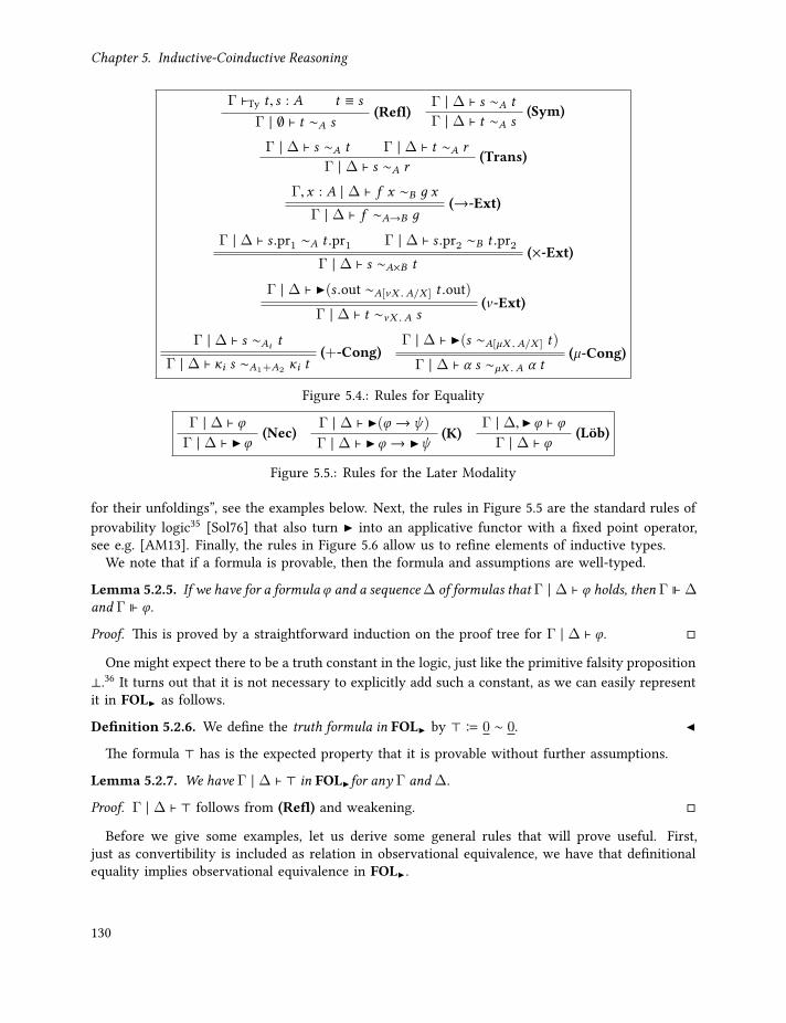
Chapter 5. Inductive-Coinductive Reasoning
Γ ⊢Ty t , s : A t ≡ s(Refl)
Γ | ∅ ⊢ t ∼A s
Γ | ∆ ⊢ s ∼A t (Sym)Γ | ∆ ⊢ t ∼A s
Γ | ∆ ⊢ s ∼A t Γ | ∆ ⊢ t ∼A r (Trans)Γ | ∆ ⊢ s ∼A r
Γ,x : A | ∆ ⊢ f x ∼B д x (→-Ext)Γ | ∆ ⊢ f ∼A→B д
Γ | ∆ ⊢ s .pr1 ∼A t .pr1 Γ | ∆ ⊢ s .pr2 ∼B t .pr2 (×-Ext)Γ | ∆ ⊢ s ∼A×B t
Γ | ∆ ⊢ (s .out ∼A[νX .A/X ] t .out)(ν-Ext)
Γ | ∆ ⊢ t ∼νX .A s
Γ | ∆ ⊢ s ∼Ai t (+-Cong)Γ | ∆ ⊢ κi s ∼A1+A2
κi t
Γ | ∆ ⊢ (s ∼A[µX .A/X ] t)(µ-Cong)
Γ | ∆ ⊢ α s ∼µX .A α t
Figure 5.4.: Rules for Equality
Γ | ∆ ⊢ ϕ(Nec)
Γ | ∆ ⊢ ϕΓ | ∆ ⊢ (ϕ → ψ )
(K)Γ | ∆ ⊢ ϕ → ψ
Γ | ∆, ϕ ⊢ ϕ(Löb)
Γ | ∆ ⊢ ϕ
Figure 5.5.: Rules for the Later Modality
for their unfoldings”, see the examples below. Next, the rules in Figure 5.5 are the standard rules ofprovability logic35 [Sol76] that also turn into an applicative functor with a fixed point operator,see e.g. [AM13]. Finally, the rules in Figure 5.6 allow us to refine elements of inductive types.
We note that if a formula is provable, then the formula and assumptions are well-typed.
Lemma 5.2.5. If we have for a formula ϕ and a sequence∆ of formulas that Γ | ∆ ⊢ ϕ holds, then Γ ⊩ ∆and Γ ⊩ ϕ.
Proof. This is proved by a straightforward induction on the proof tree for Γ | ∆ ⊢ ϕ.
One might expect there to be a truth constant in the logic, just like the primitive falsity proposition⊥.36 It turns out that it is not necessary to explicitly add such a constant, as we can easily representit in FOL as follows.
Definition 5.2.6. We define the truth formula in FOL by ⊤ B 0 ∼ 0.
The formula ⊤ has is the expected property that it is provable without further assumptions.
Lemma 5.2.7. We have Γ | ∆ ⊢ ⊤ in FOLfor any Γ and ∆.
Proof. Γ | ∆ ⊢ ⊤ follows from (Refl) and weakening.
Before we give some examples, let us derive some general rules that will prove useful. First,just as convertibility is included as relation in observational equivalence, we have that definitionalequality implies observational equivalence in FOL .
130

5.2. A First-Order Logic for Observational Equivalence
Γ | ∆[⟨ ⟩/x ] ⊢ ϕ[⟨ ⟩/x ](1-Ref)
Γ,x : 1 | ∆ ⊢ ϕ
Γ,y : A | ∆[κ1 y/x ] ⊢ ϕ[κ1 y/x ] Γ,y : B | ∆[κ2 y/x ] ⊢ ϕ[κ2 y/x ] (+-Ref)Γ,x : A+ B | ∆ ⊢ ϕ
Γ,y : A[µX .A/X ] | ∆[α y/x ] ⊢ ϕ[α y/x ](µ-Ref)
Γ,x : µX .A | ∆ ⊢ ϕ
Figure 5.6.: Refinement Rules
Lemma 5.2.8. The following rule can be derived in FOL for all terms s and t with Γ ⊢Ty s, t : A.
Γ | ∆ ⊢ s A t
Γ | ∆ ⊢ s ∼A t
Proof. We put ϕ B s ∼ x , so that Γ,x : A ⊩ ϕ and Γ | ∅ ⊢ ϕ[s/x ] by (Refl). Note that ∆[t/x ] = ∆,as x is not in ∆. Through repeatedly applying (Weak), we obtain Γ | ∆ ⊢ ϕ[s/x ]. Finally, we use(-Repl) and Γ | ∆ ⊢ s A t to deduce Γ | ∆ ⊢ ϕ[t/x ]. Since ϕ[t/x ] = s ∼ t , we get Γ | ∆ ⊢ s ∼ t .
Second, we can obtain a few structural rules related to terms and term variables.37
Lemma 5.2.9. In FOL weakening for term variables is derivable for any type A ∈ Ty:
Γ | ∆ ⊢ ϕΓ,x : A | ∆ ⊢ ϕ
Moreover, the following substitution rule is derivable.
Γ,x : A | ∆ ⊢ ϕ Γ ⊢Ty u : A(Subst)
Γ | ∆[u/x ] ⊢ ϕ[u/x ]
We also have the following exchange rule:
Γ | ∆1,ϕ1,ϕ2,∆2 ⊢ ψ (Exch)Γ | ∆1,ϕ2,ϕ1,∆2 ⊢ ψ
Finally, we can derive the following conversion rule, which is a weak form of replacement.
Γ | ∆[s/x ] ⊢ ϕ[s/x ] s ≡ t(Conv)
Γ | ∆[t/x ] ⊢ ϕ[t/x ]
Proof. All the rules weakening, substitution, exchanges and conversion, are derived by induction onthe proof trees. Most steps in these induction proofs are direct, so we only go through the criticalcases here. For weakening, (Refl) is the crucial case, in which we use that the underlying termlanguage has weakening as follows. If Γ | ∅ ⊢ t ∼B s is given by (Refl) from Γ ⊢Ty t , s : B and t ≡ s ,then also Γ,x : A ⊢Ty t , s : B and Γ,x : A | ∅ ⊢ t ∼B s by (Refl). For (Subst), the (Refl) rule is againthe crucial case, where we use that s ≡ t implies s[u/x ] ≡ t [u/x ]. For proving (Exch), on the other
131

Chapter 5. Inductive-Coinductive Reasoning
hand, the important cases are (Proj), (→-I) and (Löb). Each of them is dealt with by using (Weak)in a standard manner. Finally, for the conversion rule (Proj), (Def) and (Refl) are the critical cases.In the (Proj)-case, we use that the reduction relation preserves types (Theorem 3.2.22), whereas boththe (Def)- and (Refl)-case are given by transitivity of conversion. This concludes the proof of allfour derived rules.
In many proofs, we will need that the later modality interacts well with other results that can beproven in FOL . For instance, if we derived an entailment ϕ ⊢ ψ , then this entailment should alsohold later, that is, ϕ ⊢ ψ should be derivable as well. This is formulated in the following lemmain a more general way, together with some useful consequences like the distribution of the latermodality over the universal quantifier.
Lemma 5.2.10. The following rule, which makes an applicative functor in the sense of [AM13], isderivable in FOL .
Γ | ∆ ⊢ (ϕ → ψ ) Γ | ∆ ⊢ ϕ(Appl)
Γ | ∆ ⊢ ψMore generally, the later modality can be distributed over rules: Let Γ,∆, ϕ1, . . . ,ϕn andψ be given, suchthat for every ∆′ the following is derivable
Γ | ∆,∆′ ⊢ ϕ1 · · · Γ | ∆,∆′ ⊢ ϕnΓ | ∆,∆′ ⊢ ψ
(5.11)
in FOL , then also the following is derivable
Γ | ∆ ⊢ ϕ1 · · · Γ | ∆ ⊢ ϕnΓ | ∆ ⊢ ψ
(5.12)
In particular, the later modality distributes over ∀-quantification and (×-Ext):
Γ | ∆ ⊢ (∀x : A.ϕ)
Γ | ∆ ⊢ ∀x : A. ϕ(5.13)
Γ | ∆ ⊢ (π1 s ∼A π1 t) Γ | ∆ ⊢ (π2 s ∼B π2 t)Γ | ∆ ⊢ (s ∼A×B t)
(5.14)
Proof. We first derive (5.12) from an arbitrary proof (R) of (5.11). Let Γ, ∆, ϕ1, . . . ,ϕn andψ be givenas in the assumption. We put ∆′ B ϕ1, . . . ,ϕn , and derive from (5.11) and repeated applications of(→-I), (K) and (→-E) the following proof.
(Proj)Γ | ∆,∆′ ⊢ ϕ1 · · · Γ | ∆,∆′ ⊢ ϕn(R)
Γ | ∆,∆′ ⊢ ψ(→-I)
Γ | ∆ ⊢ ϕ1 → · · · → ϕn → ψ(Nec)
Γ | ∆ ⊢ (ϕ1 → · · · → ϕn → ψ )(K)
Γ | ∆ ⊢ ϕ1 → · · · → ϕn → ψ Γ | ∆ ⊢ ϕ1 · · · Γ | ∆ ⊢ ϕn(→-E)Γ | ∆ ⊢ ψ
132
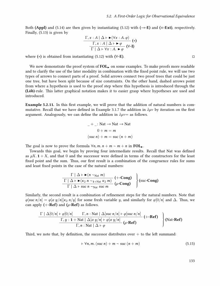
5.2. A First-Order Logic for Observational Equivalence
Both (Appl) and (5.14) are then given by instantiating (5.12) with (→-E) and (×-Ext), respectively.Finally, (5.13) is given by
Γ,x : A | ∆ ⊢ (∀x : A.ϕ)(∗)
Γ,x : A | ∆ ⊢ ϕ(∀-I)
Γ | ∆ ⊢ ∀x : A. ϕ
where (∗) is obtained from instantiating (5.12) with (∀-E).
We now demonstrate the proof system of FOL on some examples. To make proofs more readableand to clarify the use of the later modality in combination with the fixed point rule, we will use twotypes of arrows to connect parts of a proof. Solid arrows connect two proof trees that could be justone tree, but have been split because of size constraints. On the other hand, dashed arrows pointfrom where a hypothesis is used to the proof step where this hypothesis is introduced through the(Löb)-rule. This latter graphical notation makes it to easier grasp where hypotheses are used andintroduced.
Example 5.2.11. In this first example, we will prove that the addition of natural numbers is com-mutative. Recall that we have defined in Example 3.1.7 the addition in λµν by iteration on the firstargument. Analogously, we can define the addition in λµν= as follows.
_+ _ : Nat→ Nat→ Nat0 +m =m
(suc n) +m = suc (n +m)
The goal is now to prove the formula ∀n,m.n +m ∼m + n in FOL .Towards this goal, we begin by proving four intermediate results. Recall that Nat was defined
as µX . 1 + X , and that 0 and the successor were defined in terms of the constructors for the leastfixed point and the sum. Thus, our first result is a combination of the congruence rules for sumsand least fixed points in the case of the natural numbers:
Γ | ∆ ⊢ (n ∼Nat m)(+-Cong)
Γ | ∆ ⊢ (κ2 n ∼1+Nat κ2m)(µ-Cong)
Γ | ∆ ⊢ suc n ∼Nat sucm
(suc-Cong)
Similarly, the second result is a combination of refinement steps for the natural numbers. Note thatϕ[suc n/n] = ϕ[α y/n][κ2 n/y] for some fresh variable y, and similarly for ϕ[0/n] and ∆. Thus, wecan apply (+-Ref) and (µ-Ref) as follows.
Γ | ∆[0/n] ⊢ ϕ[0/n] Γ,n : Nat | ∆[suc n/n] ⊢ ϕ[suc n/n](+-Ref)
Γ,y : 1+ Nat | ∆[α y/n] ⊢ ϕ[α y/n](µ-Ref)
Γ,n : Nat | ∆ ⊢ ϕ
(Nat-Ref)
Third, we note that, by definition, the successor distributes over + to the left summand:
⊢ ∀n,m. (suc n) +m ∼ suc (n +m) (5.15)
133

Chapter 5. Inductive-Coinductive Reasoning
by the following proof in FOL .
(suc n) +m ≡ suc (n +m)(Refl)
n,m : Nat | ∅ ⊢ (suc n) +m ∼ suc (n +m)(∀-I)⊢ ∀n,m. (suc n) +m ∼ suc (n +m)
Lastly, the analogous property for the right summand, that is
⊢ ∀n,m.n + (sucm) ∼ suc (n +m), (5.16)
also holds as follows. First, we note that the definition of + gives us the following computations.
0 + sucm ≡ sucm ≡ suc (0 +m) (5.17)(suc n) + (sucm) ≡ suc(n + (sucm)) (5.18)suc ((suc n) +m) ≡ suc (suc (n +m)) (5.19)
The proof of the successor distribution to the right is our first proof that uses the (Löb)-rule. Asdiscussed, we indicate the recursion step by a dashed arrow in the proof. We put Γ B n,m : Natand ∆ B (∀n,m.n + (sucm) ∼ suc (n +m)), and prove (5.16) by induction on n as follows.
(5.17)
(Proj), (∀-E)Γ | ∆ ⊢ (n + (sucm) ∼ suc (n +m))
(suc-Cong)Γ | ∆ ⊢ suc (n + (sucm)) ∼ suc (suc (n +m)) (5.18), (5.19)
(Conv)Γ | ∆ ⊢ (suc n) + (sucm) ∼ suc ((suc n) +m)
(Nat-Ref)Γ | ∆ ⊢ n + (sucm) ∼ suc (n +m)
(∀-I)n : Nat | ∆ ⊢ ∀m.n + (sucm) ∼ suc (n +m)
(∀-I)∆ ⊢ ∀nm.n + (sucm) ∼ suc (n +m)
(Löb)⊢ ∀nm.n + (sucm) ∼ suc (n +m)
Finally, we can put the above results together to prove commutativity of addition. In the proofbelow we use the assumptions ∆ and the context Γ, given by ∆ B (∀n,m.n +m ∼ m + n) andΓ B n,m : Nat, respectively. The proof of commutativity is given as follows.
Γ | ∆ ⊢ 0 + 0 ∼ 0 + 0
(Proj), (5.13), (∀-E)Γ | ∆ ⊢ (0 +m ∼m + 0)
(suc-Cong)Γ | ∆ ⊢ suc (0 +m) ∼ suc (m + 0)
(5.16), (Trans), (5.15)Γ | ∆ ⊢ 0 + (sucm) ∼ (sucm) + 0
(Nat-Ref)Γ | ∆ ⊢ 0 +m ∼m + 0
Γ | ∆ ⊢ 0 +m ∼m + 0
(Proj), (5.13), (∀-E)Γ | ∆ ⊢ (n +m ∼m + n)
(suc-Cong)Γ | ∆ ⊢ suc (n +m) ∼ suc (m + n)
(5.15), (Trans), (5.16)Γ | ∆ ⊢ (suc n) +m ∼m + (suc n)
(Nat-Ref)Γ | ∆ ⊢ n +m ∼m + n (Löb) + (∀-I)⊢ ∀n,m.n +m ∼m + n
134

5.2. A First-Order Logic for Observational Equivalence
Note that we used two recursion steps in this proof, as the proof proceeds by induction both on nand on m. Traditionally, this proof would be broken up into two separate induction proofs to fitthe usual induction scheme. However, in the present setup we can just follow the natural steps thatarise in the proof.
Let us now use FOL to prove some equivalences on coinductive types. In the first example, welook again at the stream equivalence that we proved in Example 5.1.11. This allows us to demonstratehow proofs by coinduction arise from combining the extensionality rules for products and greatestfixed points, and the (Löb)-rule.
Example 5.2.12. Recall from Example 3.2.11 that we have defined a map that selects the oddpositions of a stream, and that we have proved in Example 5.1.11 that the application of this map tothe alternating bit stream results in a constant stream. In Example 5.1.11, we used the bisimulationproof method to show this equivalence. We will now prove it again but this time around in FOL .That is, we show that the formula select oddF alt ∼ 1ω is derivable in FOL .
Intuitively, to show that two streams are equivalent, we need to show that their heads matchand their tails continue to be equivalent. This extensionality principle for streams can be derived inFOL , similarly to the refinement rule for natural numbers:
Γ | ∆ ⊢ s .hd ∼A t .hd(Nec)Γ | ∆ ⊢ (s .hd ∼A t .hd) Γ | ∆ ⊢ (s .tl ∼Aω t .tl)
(5.14)Γ | ∆ ⊢ (s .out ∼ t .out)
(ν-Ext)Γ | ∆ ⊢ s ∼Aω t
(Aω -Ext)
Combined with the fixed point rule (Löb), this extensionality principle allows us to prove streamequivalences, as we will demonstrate now.
We want to show that select oddFalt ∼ 1ω is derivable. This is accomplished by the following proof,in which we use ∆ given by ∆ B (select oddF alt ∼ 1ω), and the following two computations.
(select oddF alt).tl ≡ select oddF alt (5.20)1ω .tl ≡ 1ω (5.21)
∆ ⊢ (select oddF alt).hd ≡ 1ω .hd∆ ⊢ (select oddF alt).hd ∼A (1ω).hd
(Proj)∆ ⊢ (select oddF alt ∼ 1ω) (5.20), (5.21)
(Conv)∆ ⊢ ((select oddF alt).tl ∼ 1ω .tl)
(Natω -Ext)∆ ⊢ select oddF alt ∼ 1ω
(Löb)⊢ select oddF alt ∼ 1ω
This proof should be compared to Example 5.1.11, where we proved that the relation R, which wasgiven by RNatω = (select oddF alt, 1ω), is an observational bisimulation up-to. However, there wehad to use a clever combination of up-to techniques, whereas in the present proof the steps that wehave to take arise naturally in the construction of the proof. It should be noted though that up-totechniques still play an important role in the semantics of FOL , see Section 5.2.2.
In the next example we prove that addition of streams is commutative. This demonstrates coin-duction for streams on a quantified formula.
135

Chapter 5. Inductive-Coinductive Reasoning
Example 5.2.13. Recall that streams of natural numbers are given by Natω = νX .Nat × X , see Ex-ample 3.1.2, and from Example 3.1.8 that stream addition is defined from addition on Nat by
_ ⊕ _ : Natω → Natω → Natω
(s ⊕ t).hd = s .hd+ t .hd(s ⊕ t).tl = s .tl ⊕ t .tl
To show that ⊕ is commutative, we first observe that by commutativity of addition on naturalnumbers (Example 5.2.11) we have for all s, t : Natω
(s ⊕ t).hd ≡ s .hd+ t .hd ∼ t .hd+ s .hd ≡ (t ⊕ s).hd, (5.22)
and from the definition of stream addition we obtain
(s ⊕ t).tl ≡ s .tl ⊕ t .tl and t .tl ⊕ s .tl ≡ (t ⊕ s).tl (5.23)
Let ∆ B (∀s, t : Natω . s ⊕ t ∼ t ⊕ s) and Γ B s, t : Natω , then the following is a proof in FOL .
(5.22)Γ | ∆ ⊢ (s ⊕ t).hd ∼ (t ⊕ s).hd
(Proj), (5.13)Γ | ∆ ⊢ ∀s, t : Natω . (s ⊕ t ∼ t ⊕ s)
(∀-E)Γ | ∆ ⊢ (s .tl ⊕ t .tl ∼ t .tl ⊕ s .tl)
(Conv), (5.23)Γ | ∆ ⊢ ((s ⊕ t).tl ∼ (t ⊕ s).tl)
(Natω -Ext)Γ | ∆ ⊢ s ⊕ t ∼ t ⊕ s (∀-I)
∆ ⊢ ∀s, t : Natω . s ⊕ t ∼ t ⊕ s (Löb)⊢ ∀s, t : Natω . s ⊕ t ∼ t ⊕ s
This shows that ⊕ is commutative.
In the final example of this section we derive the FOL-version of the induction principle fornatural numbers.
Example 5.2.14. Recall from Definition 5.2.2 that for formula ϕ with Γ,n : Nat ⊩ ϕ, we denote fort : Nat the formula ϕ[t/n] by ϕ[t ]. Usually, the induction principle for natural numbers reads like
Γ ⊢ ϕ[0] Γ,m : Nat | ϕ[m] ⊢ ϕ[sucm]
Γ,n : Nat ⊢ ϕ
In the context of the logic FOL , we cannot derive the rule in this form but we need to introducea later modality on the induction hypothesis:
Γ | ∆ ⊢ ϕ[0] Γ | ∆ ⊢ ∀n : Nat. ϕ[n]→ ϕ[suc n](Nat-Ind)
Γ | ∆ ⊢ ∀n : Nat.ϕ
This rule can be derived by using the fixed point rule and the refinement rules as in the following
136
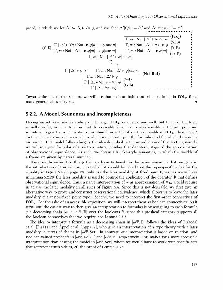
5.2. A First-Order Logic for Observational Equivalence
proof, in which we let ∆′ B ∆, ∀n.ϕ, and use that ∆′[0/n] = ∆′ and ∆′[suc n/n] = ∆′.
Γ | ∆′ ⊢ ∀n : Nat. ϕ[n]→ ϕ[suc n](∀-E)
Γ,m : Nat | ∆′ ⊢ ϕ[m]→ ϕ[sucm]
(Proj)Γ,m : Nat | ∆′ ⊢ ∀n.ϕ
(5.13)Γ,m : Nat | ∆′ ⊢ ∀n. ϕ
(∀-E)Γ,m : Nat | ∆′ ⊢ ϕ[m]
(→-E)Γ,m : Nat | ∆′ ⊢ ϕ[sucm]
Γ | ∆′ ⊢ ϕ[0] Γ,m : Nat | ∆′ ⊢ ϕ[sucm](Nat-Ref)
Γ,n : Nat | ∆′ ⊢ ϕ(∀-I)
Γ | ∆, ∀n.ϕ ⊢ ∀n.ϕ(Löb)
Γ | ∆ ⊢ ∀n.ϕTowards the end of this section, we will see that such an induction principle holds in FOL for amore general class of types.
5.2.2. A Model, Soundness and IncompletenessHaving an intuitive understanding of the logic FOL is all nice and well, but to make the logicactually useful, we need to show that the derivable formulas are also sensible in the interpretationwe intend to give them. For instance, we should prove that if s ∼ t is derivable in FOL , then s ≡obs t .To this end, we construct a model, in which we can interpret the formulas and for which the axiomsare sound. This model follows largely the idea described in the introduction of this section, namelywe will interpret formulas relative to a natural number that denotes a stage of the approximationof observational equivalence. As such, we obtain a Kripke-style semantics, in which the worlds ofa frame are given by natural numbers.
There are, however, two things that we have to tweak on the naive semantics that we gave inthe introduction of this section. First of all, it should be noted that the type-specific rules for theequality in Figure 5.4 on page 130 only use the later modality at fixed point types. As we will seein Lemma 5.2.28, the later modality is used to control the application of the operator Φ that definesobservational equivalence. Thus, a naive interpretation of ∼ as approximation of ≡obs would requireus to use the later modality in all rules of Figure 5.4. Since this is not desirable, we first give analternative way to prove and construct observational equivalence, which allows us to leave the latermodality out at non-fixed point types. Second, we need to interpret the first-order connectives ofFOL . For the sake of an accessible exposition, we will interpret them as Boolean connectives. As itturns out, the easiest way to then give an interpretation to formulas is by assigning to each formulaϕ a decreasing chain JϕK ∈ [ωop,B] over the booleans B, since this presheaf category supports allthe Boolean connectives that we require, see Lemma 2.3.3.
The idea to interpret a formula as a decreasing chain in [ωop,B] follows the ideas of Birkedalet al. [Bir+11] and Appel et al. [App+07], who give an interpretation of a type theory with a latermodality in terms of chains in [ωop, Set]. In contrast, our interpretation is based on relation- andBoolean-valued presheafs in [ωop,RelΛ= ] and [ωop,B], respectively. This makes for a more accessibleinterpretation than casting the model in [ωop, Set], where we would have to work with specific setsthat represent truth-values, cf. the proof of Lemma 2.3.3.
137
Chapter 5. Inductive-Coinductive Reasoning
Notation 5.2.15. Since we focus on terms in the copattern calculus λµν= in this chapter, we abusenotation and write Rel instead of RelΛ= for the complete lattice of (type-indexed) binary relationsover terms in λµν=.
In what follows, we need to characterise the components of closed types.
Lemma 5.2.16. Let A be a closed type. Then either there are closed types B and C , such that A = B ×C ,A = B +C or A = B → C , or there is X ⊩ B : Ty and ρ ∈ µ,ν with A = ρX . B. In the first case, werefer to B and C as the components of A.
Proof. This follows directly by induction on the derivation of ⊩ A : Ty.
As we mentioned already above, we need a different way of proving observational equivalencethat allows us to leave out intermediate steps in a bisimulation. For example, if we want to provethat R is an observational bisimulation at the type of streams over A, then the results in Section 5.1.2require us to show for all (s, t) ∈ RAω that (s .out, t .out) ∈ Cobs(R)A×Aω . Typically, we are onlyinterested in the head and tail of streams though. Thus, it would be more natural to leave out theintermediate step and only require that (s .hd, t .hd) ∈ Cobs(R)A and (s .tl, t .tl) ∈ Cobs(R)Aω . We canachieve this simplification by using the following notion of compressed bisimulation. Note that theuse of compressed bisimulations is very similar to the use of Φ as an up-to technique.
Definition 5.2.17. Let Φc : Rel→ Rel be the operator defined by
Φc (R)A =
Φ(R)A, A = ρX . B, ρ ∈ µ,ν Φ(Φc (R))A, otherwise.
A compressed observational bisimulation, Φc -bisimulation for short, is a relation R ∈ Rel, such thatR ⊑ Φc (R).
Note that Φc in Definition 5.2.17 is well-defined because in the second clause A is a product, asum or a function space, hence Φ only refers to the components of these types, see Definition 5.1.6and Lemma 5.1.8. For instance, if A = B → C , then we have that
Φc (R)B→C = Φ(Φc (R))B→C = (t1, t2) | (δ(t1),δ(t2)) ∈ F (Φc (R))B→C = (t1, t2) | (δ(t1),δ(t2)) ∈ ⟨F (π1), F (π2)⟩(F (Φc (R)))B→C
and since F (Φc (R))B→C = P(Φc (R)B)ONA , the definition of Φc (R)B→C only depends on Φc (R)B . By
Lemma 5.2.16 we eventually arrive at the first case.As one might expect, a compressed observational bisimulation can be completed to an actual
observational bisimulation. For instance, in the stream example we can add all pairs (s .out, t .out),for which (s, t) ∈ R, (s .hd, t .hd) ∈ Cobs(R)A and (s .tl, t .tl) ∈ Cobs(R)Aω . Instead of constructing sucha bisimulation, we can show directly that a Φc -bisimulation is a Φ-bisimulation up to γΦ, whereγΦ is the companion of Φ from Definition 2.5.12. This approach significantly simplifies the proofbecause the construction of a Φ-bisimulation from a Φc -bisimulation is quite involved.
Lemma 5.2.18. If R is a Φc -bisimulation, then R is a Φ-bisimulation up to γΦ. Thus, if two terms s andt are related by R, then s ≡obs t .
138

5.2. A First-Order Logic for Observational Equivalence
Proof. Let R be a Φc -bisimulation. We prove RA ⊆ Φ(γΦ(R))A by induction on A, see Lemma 5.2.16.If A is a fixed point type, that is, if A = ρX . B, then
RA ⊆ Φc (R)A = Φ(R)A ⊆ Φ(γΦ(R))A,
by the assumption that R is a Φc -bisimulation, the definition of Φc and id ⊑ γΦ (Lemma 2.5.13).Otherwise, if A is not a fixed point type, then
RA ⊆ Φc (R)A = Φ(Φc (R))A ⊆ Φ(Φ(γΦ(R)))A ⊆ Φ(γΦ(R))A,
by definition of Φc , the induction hypothesis that RB ⊆ Φ(γΦ(R))B for components B of A, andΦ ⊑ γΦ (Lemma 2.5.13). Thus, R ⊑ Φ(γΦ(R)) as required.
We are now in the position to construct a model for the logic FOL . Since formulas of the forms ∼ t will be interpreted in the approximations of Φc -bisimilarity, the first step is to define theseapproximations.
Definition 5.2.19. The chain of approximations of compressed observational bisimilarity is thesequence ←−−Φc ∈ [ωop,Rel] defined inductively by
←−−Φc (0) B I B Λ= × Λ=
←−−Φc (n + 1) B Φc
(←−−Φc (n)
).
Note that this is indeed an ωop-chain because ←−−Φc (I)(n) ⊒←−−Φc (I)(n + 1) for all n ∈ N by I ⊒ Φ(I)
and monotonicity of Φc .
The crucial result is now that we can prove observational equivalence of two terms by provingthat they are related by every approximation of Φc -bisimilarity.
Lemma 5.2.20. Let A be a type in Ty and s, t terms in Λ=(A). If (s, t) ∈ ←−−Φc (n)A for all n ∈ N, thens ≡obs t .
Proof. One first proves that Φc is ωop-continuous, that is, for any family Ri i ∈N of ≡-closed relationsRi ∈ Rel with Ri+1 ⊑ Ri , we have Φc (
di ∈N Ri ) =
di ∈NΦc (Ri ). This follows easily from the
characterisation of Φ in Lemma 5.1.8, where care has to be taken only in the case of inductive types.There, the limit preservation crucially requires confluence of the reduction relation in λµν=. SinceΦc is ωop-continuous, the chain ←−−Φc stabilises, see Definition 2.5.5. Thus, by Lemma 2.5.6, we getthat the largest fixed point νΦc ∈ Rel of Φc is given as νΦc =
dn∈N←−−Φc (n), see also [CC79; San09].
Thus, s and t are related by νΦc if and only if they are related by ←−Φ(n) for every n. Since νΦc is aΦc -bisimulation, we obtain s ≡obs t from Lemma 5.2.18.
Recall from Lemma 2.3.3 that B = tt, ff is the two-valued Boolean algebra and that [ωop,B] isCartesian closed, complete and cocomplete (Proposition 2.3.2). For brevity, we denote this categoryby
T B [ωop,B] . (5.24)
139
Chapter 5. Inductive-Coinductive Reasoning
Given a set I , we denote the I -indexed product and coproduct by∧· I : TI → T and
∨· I : TI → T,respectively. If I is a two element set, then we denote the resulting binary product and coproductby ∧· and ∨· . Completeness and cocompleteness also give rise to initial and terminal objects that aregiven by
∀n ∈ N. 0(n) = ff and 1(n) = tt.
Finally, the exponential in T is denoted by ⇒ : Top × T→ T, see the discussion after Lemma 2.3.3.To make the semantics of the logic more readable, we interpret the membership for pairs of terms
in the chain ←−−Φc as a chain in T as follows.
Definition 5.2.21. For a type A ∈ Ty and terms s, t ∈ Λ=(A), we define a chain s ≈c t ∈ T:
∀n ∈ N. (s ≈c t)(n) B (s, t) ∈ ←−−Φc (n)A. (5.25)
That s ≈c t is a chain in T follows directly from the fact that ←−−Φc ∈ [ωop,Rel].
The model of FOL is now given by the following Kripke-style semantics. Here, ▷ : T→ T is thefunctor with (▷ ζ )(0) = tt and (▷ ζ )(k + 1) = ζ (k) that we introduced in Lemma 2.3.4. Moreover,we denote by λλ the introduction of a set-theoretic function.
Definition 5.2.22. Let ϕ be a formula of FOL with Γ ⊩ ϕ, see Definition 5.2.1. We define forσ ∈ Subst(ON; Γ) a chain JϕK(σ) ∈ T by induction on ϕ.
J⊥K(σ) B 0Js tK(σ) B λλn. s[σ ] ≡ t [σ ]Js ∼ tK(σ) B s[σ ] ≈c t [σ ]JϕK(σ) B ▷JϕK(σ)Jϕ ∧ψ K(σ) B JϕK(σ) ∧· Jψ K(σ)Jϕ ∨ψ K(σ) B JϕK(σ) ∨· Jψ K(σ)Jϕ → ψ K(σ) B JϕK(σ)⇒ Jψ K(σ)J∀x : A.ϕK(σ) B ∧· t ∈ONAJϕK(σ [x 7→ t ])J∃x : A.ϕK(σ) B ∨· t ∈ONAJϕK(σ [x 7→ t ])
Suppose ∆ is a sequence of formulas with Γ ⊩ ∆. Given n ∈ N, a formula ϕ and σ ∈ Subst(ON; Γ),we write
σ ;n ⊨ ϕ B JϕK(σ)(n),and say that ϕ is satisfied at stage n and σ . Next, given a sequence ∆ of formulas we say that ϕ issatisfied under the assumption in ∆ at σ , if whenever all the formulas in ∆ are satisfied, then ϕ issatisfied:
∆;σ ;n ⊨ ϕ B if (∀ψ ∈ ∆. σ ;n ⊨ ψ ), then σ ;n ⊨ ϕ.
Finally, we say that ϕ is satisfied under the assumptions in ∆, if ∆;σ ;n ⊨ ϕ holds for all σ :
Γ | ∆;n ⊨ ϕ B ∀σ ∈ Subst(ON; Γ).∆;σ ;n ⊨ ϕ
140

5.2. A First-Order Logic for Observational Equivalence
We note for ζ ∈ T that ∀n ∈ N. ζ (n) holds if and only if there exists a morphism 1 → ζ in T.Thus, we frequently use the equivalence
∀n ∈ N.n ⊨ ϕ holds iff the hom-set T(1, JϕK) is inhabited.
The following proposition provides a more general formulation of this fact.
Proposition 5.2.23. Given a sequence ∆ of formulas, a formula ϕ and a substitution σ , we have that
there is a morphism(∧· ψ ∈∆Jψ K(σ)) → JϕK(σ) in T iff ∀n ∈ N.∆ |;σ ;n ⊨ ϕ.
We now show in a series of lemmas that the axioms of FOL are sound for the interpretation inDefinition 5.2.22. The final result we aim for is the following theorem.
Theorem 5.2.24. The axioms of FOL are sound for the interpretation in Definition 5.2.22, in the sensethat for all formulas ϕ,
if Γ | ∆ ⊢ ϕ, then ∀n ∈ N. Γ | ∆;n ⊨ ϕ.
In particular, if ⊢ s ∼ t , then s ≡obs t .
The first step towards proving Theorem 5.2.24 is to show the validity of the rules that make ∼an equivalence relation. We prove this by appealing to the following result that allows us to inferproperties of the approximations ←−Φ from compatible up-to techniques, for which we recall fromDefinition 2.5.10 that Φ×mc : Lm → Lm is given by point-wise application of Φc .
Lemma 5.2.25. Let T : Relm → Rel be Φc -compatible, that is T Φ×mc ⊑ Φc T . Then we haveT (←−−Φc (n)
m) ⊑ ←−−Φc (n) for all n ∈ N.
Proof. We proceed by induction on n. If n = 0, then ←−−Φc (0) = I and the claim holds trivially.Otherwise, assume that T (←−−Φc (n)
m) ⊑ ←−−Φc (n) holds for n ∈ N, and we prove T (←−−Φc (n + 1)m) ⊑
←−−Φc (n + 1). Indeed, we have
T (←−−Φc (n + 1)m) = T (Φc (
←−−Φc (n))
m)
⊑ Φc (T (←−−Φc (n)
m)) by compatibility
⊑ Φc (←−−Φc (n)) by IH and monotonicity of Φc
=←−−Φc (n + 1)
Thus, by induction, T (←−−Φc (n)m) ⊑ ←−−Φc (n) holds for all n ∈ N.
Since we have already investigated some up-to techniques for Φ, we wish to reuse these techniquesfor compressed bisimulations. The following result allows us to transfer compatibility of up-totechniques for Φ to Φc , if the up-to technique in question is given on each type separately.
Lemma 5.2.26. LetT : Relm → Rel beΦ-compatible and assume thatT factors through a family of mapsSA : RelmΛ=(A) → RelΛ=(A)A∈Ty, in the sense that for any m-tuple of relations
#—R , we have T
( #—R
)A =
SA( # —RA
). Under these conditions, T is also Φc -compatible.
141

Chapter 5. Inductive-Coinductive Reasoning
Proof. We show that for any m-tuple #—R of relations and type A that T
(Φ×mc
( #—R
) )A ⊆ Φc
(T
( #—R
) )A by
induction on A. If A = ρX . B, then
T(Φ×mc
( #—R
) )A = SA
(Φ×mc
( #—R
)A
)by factorisation of T
= SAΦ×m ( #—
R)A by definition of Φc
= T(Φ×m
( #—R
) )A by factorisation of T
⊆ Φ(T( #—R
) )A by compatibility
= Φc(T
( #—R
) )A by definition of Φc .
Otherwise, if A is not a fixed point type, then we have
T(Φ×mc
( #—R
) )A = SA
(Φ×mc
( #—R
)A
)= SA
(Φ×m
(Φ×mc
( #—R
) )A
)= T
(Φ×m
(Φ×mc
( #—R
) ) )A by factorisation T
⊆ Φ(T(Φ×mc
( #—R
) ) )A by compatibility
⊆ Φ(Φc
(T
( #—R
) ) )A by induction Hyp.
= Φc(T
( #—R
) )A by definition of Φc .
Thus T(Φ×mc
( #—R
) )A ⊆ Φc
(T
( #—R
) )A holds for all #—
R and A, hence T is Φc -compatible.
We now use Lemma 5.2.25 to obtain soundness of the rules (Refl), (Sym) and (Trans).
Lemma 5.2.27. The chain ≈c is an equivalence relation and is closed under conversion at each stage.More precisely, for all A ∈ Ty and r , s, t ,u ∈ Λ=(A), there are the following morphisms in T.
1. 1→ t ≈c t (Reflexivity);
2. s ≈c t → t ≈c s (Symmetry);
3. r ≈c s ∧ s ≈c t → r ≈c t (Transitivity); and
4. s ≈c t → r ≈c u, if r ≡ s and t ≡ u (Conversion closure).
Proof. We prove 1–4 by formulating these properties so that we can apply Lemma 5.2.25. This isachieved by using the maps Refl : 1→ Rel, Sym : Rel→ Rel, _ ;_ : Rel×Rel→ Rel and C≡ : Rel→ Rel,where Refl maps constantly to the diagonal relation Eq, Sym maps a relation to its inverse, _ ; _is the composition of relations, and C≡ closes a relation under conversion. The statement of 1–4 is then equivalent to saying for all n ∈ N that Refl
(←−−Φc (n)
)⊑ ←−−Φc (n), Sym
(←−−Φc (n)
)⊑ ←−−Φc (n),
←−−Φc (n) ;
←−−Φc (n) ⊑
←−−Φc (n) and C≡
(←−−Φc (n)
)⊑ ←−−Φc (n). It remains to show that the maps Refl, Sym,
_ ; _ and C≡ are Φc -compatible, since we then can appeal to Lemma 5.2.25 to obtain the aboveinclusions. Towards this end, one first shows that these maps are Φ-compatible. Compatibility ofreflexivity, symmetry and composition has been proved in [Bon+14, Sec 4.2], which uses that Φ isthe canonical relation lifting of F , see Definition 5.1.6 and that F preserves weak pullbacks. Weakpullback preservation follows directly from the definition of F in terms of products, coproducts, andthe power set functor, see [GS00]. For compatibility of the ≡-closure we use that for any relation
142

5.2. A First-Order Logic for Observational Equivalence
C≡(R) ⊑ C≡obs(R) and that C≡obs is compatible, see Proposition 5.1.10. Finally, Φc -compatibility ofthe maps follows from Lemma 5.2.26, as the maps Refl, Sym, _ ; _ and C≡ are defined on each typeseparately.
The next step is to establish the soundness of the extensionality and congruence rules for ∼. Sincethe rules (ν-Ext) and (µ-Cong) involve the later modality, we first show how this modality can beinterpreted over [ωop,Rel] and how it can be used to “guard”, cf. [BM13], the unfolding of ←−−Φc .
Lemma 5.2.28. Let Φc : [ωop,Rel] → [ωop,Rel] be given by Φc (S)(n) B Φc (S(n)). We have for thefunctor ▷ : [ωop,Rel]→ [ωop,Rel] defined in Lemma 2.3.4 that
←−−Φc = ▷(Φc (
←−−Φc )). (5.26)
Proof. To show that ←−−Φc = ▷(Φc (←−−Φc )) for the ←−−Φc from Definition 5.2.19, let n ∈ N. Then by
Lemma 2.3.4
▷(Φc (←−−Φc )
)(n) =
I, n = 0
Φc (←−−Φc )(k), n = k + 1
=
I, n = 0
Φc (←−−Φc (k)), n = k + 1
=
I, n = 0←−−Φc (k + 1), n = k + 1
=←−−Φc (n).
Thus, ▷(Φc (←−−Φc ))(n) =
←−−Φc (n) for all n ∈ N and so ←−−Φc = ▷(Φc (
←−−Φc )).
Lemma 5.2.29. The rules (→-Ext), (×-Ext), (ν-Ext), (+-Cong) and (µ-Cong) are sound for the inter-pretation in Definition 5.2.22. More precisely, the following are isomorphisms in T.
(s ≈c t) ∧·
u ∈ONA
s u ≈c t u ∀s, t : A→ B
(s ≈c t) (π1 s ≈c π1 t) ∧ (π2 s ≈c π2 t) ∀s, t : A × B(s ≈c t) ▷(t .out ≈c s .out) ∀s, t : νX .A
(κi s ≈c κi t) (t ≈c s) ∀i ∈ 1, 2 and s, t : Ai
(α s ≈c α t) ▷(t ≈c s) ∀s, t : A[µX .A/X ]
Proof. We show that the premises of the rules imply the corresponding conclusion in each case.
• For function typesA→ B, we first note that for s, t ∈ Λ=(A→ B) the existence of an isomorph-ism (s ≈c t)
∧· u ∈ONA s u ≈c t u simply means that for all n ∈ N, (s, t) ∈ ←−−Φc (n)A→B ⇐⇒
∀u ∈ ONA. (s u, t u) ∈←−−Φc (n)B . For 0 this is trivial since ←−−Φc (0) = I. On the other hand, for
n ∈ N we have←−−Φc (n + 1)A→B = Φc (
←−−Φc (n))A→B = Φ(Φc (
←−−Φc (n)))A→B = Φ(
←−−Φc (n + 1))A→B .
By Lemma 5.1.8 (s, t) ∈ Φ(←−−Φc (n + 1))A→B is equivalent to ∀u ∈ ONA. (s u, t u) ∈←−−Φc (n + 1)
because ←−−Φc is ≡-closed, see Lemma 5.2.27. Thus the desired isomorphism exists.
143

Chapter 5. Inductive-Coinductive Reasoning
• The proof of soundness for (×-Ext) and (+-Cong) is analogous to that for (→-Ext).
• To prove soundness of (ν-Ext) and (µ-Cong), we appeal to the identity ←−−Φc = ▷(Φc (←−−Φc )
)from Lemma 5.2.28 as follows. Suppose we are given s, t ∈ Λ=(νX .A) and n ∈ N. Then wehave
(s, t) ∈ ▷(Φc (←−−Φc )
)(n)νX .A ⇐⇒
(s, t) ∈ IνX .A, n = 0
(s, t) ∈ Φ(←−−Φc (k))νX .A, n = k + 1
⇐⇒(s .out, t .out) ∈ IA[νX .A/X ], n = 0
(s .out, t .out) ∈ ←−−Φc (k)A[νX .A/X ], n = k + 1(∗)
⇐⇒ (s .out, t .out) ∈ (▷←−−Φc )(n)A[νX .A/X ],
where we can apply Lemma 5.1.8 in the second case of (∗), since ←−−Φc is closed under convert-ibility. Combining this relation with (5.26) from Lemma 5.2.28, we obtain
(s ≈c )(n) ⇐⇒ (s, t) ∈ ←−−Φc (n)
⇐⇒ (s, t) ∈(▷Φc (
←−−Φc )
)(n) by (5.26)
⇐⇒ (s .out, t .out) ∈ (▷←−−Φc )(n) see above⇐⇒ ▷(s .out ≈c t .out)(n)
which shows that (ν-Ext) is sound.
• Similarly, one shows for s, t ∈ Λ=(A[µX .A/X ]) and n ∈ N that
(α s,α t) ∈(▷Φc (
←−−Φc )
)(n) ⇐⇒ (s, t) ∈ (▷←−−Φc )(n),
from which we obtain soundness of (µ-Cong) by the same reasoning as for (ν-Ext).
Now that we have proven that the axioms for ∼ are correct, we are left with the task to showsoundness of the axioms for the later modality (Figure 5.5 on page 130) and of the refinement rules(Figure 5.6, page 131). The rules (K) and (Nec) for the later modality are instances of the functorialityof ▷ and the next operator in Lemma 2.3.4 for the category T. The soundness of the fixed point rule(Löb) has been proven in Lemma 2.3.5.
To prove the refinement rules correct, we first show that we can replace convertible terms informulas without affecting their validity. Conveniently, this also proves soundness of the replacementrule for definitional equality.
Lemma 5.2.30. Let ϕ be a formula with Γ ⊩ ϕ and σ ,τ ∈ Subst(ON; Γ). If σ ≡ τ , that is σ(x) ≡ τ (x)for all x ∈ dom(Γ), then JϕK(σ) JϕK(τ ).Proof. We proceed by induction on the formula ϕ. By applying Lemma 5.2.27 to s[σ ] ≡ s[τ ] andt [σ ] ≡ t [τ ], we have for all terms s and t that Js ∼ tK(σ) Js ∼ tK(τ ), which proves the claim in thebase case ϕ = s ∼ t . All the other cases follow immediately by induction from functoriality of theoperations that we used in the definition of J−K in Definition 5.2.22.
144
5.2. A First-Order Logic for Observational Equivalence
Lemma 5.2.30 allows us now to replace terms of inductive type by their weak head normal forms,which allows us to obtain soundness for the refinement rules.
Lemma 5.2.31. The rules (1-Ref), (+-Ref) and (µ-Ref) are sound for the interpretation in Defini-tion 5.2.22, that is, for all n ∈ N we have
i) if Γ | ∆[⟨ ⟩/x ];n ⊨ ϕ[⟨ ⟩/x ], then Γ,x : 1 | ∆;n ⊨ ϕ;
ii) if Γ,yi : Ai | ∆[κi yi/x ];n ⊨ ϕ[κi yi/x ] for all i ∈ 1, 2, then Γ,x : A1 +A2 | ∆;n ⊨ ϕ;
iii) if Γ,y : A[µX .A/X ] | ∆[α y/x ];n ⊨ ϕ[α y/x ], then Γ,x : µX .A | ∆;n ⊨ ϕ.
Proof. Suppose that ϕ is a formula with Γ,x : A1 + A2 ⊩ ϕ, and let us assume for all n ∈ N thatΓ,yi : Ai | ∆[κi yi/x ];n ⊨ ϕ[κi yi/x ] holds for all i ∈ 1, 2. We need to show that Γ,x : A1 + A2 |∆;n ⊨ ϕ holds for all n ∈ N. Thus, by Proposition 5.2.23, we need to show that if for all i ∈ 1, 2and all τ ∈ Subst(ON; Γ,x : Ai ), there are morphisms
∧· ψ ∈∆Jψ [κi yi/x ]K(τ )→ Jϕ[κi yi/x ]K(τ ), then
for all σ ∈ Subst(ON; Γ,x : A1 +A2), there is∧· ψ ∈∆Jψ K(σ)→ JϕK(σ).
So let σ ∈ Subst(ON; Γ,x : A1 +A2). Since σ(x) ∈ ONA1+A2, there is an i ∈ 1, 2 and a t with
σ(x) ≡ κi t . We then define τ B σ [x 7→ κi t ] and γ B σ [yi 7→ t ], so that ∆[κi yi/x ][γ ] = ∆[τ ] andϕ[κi yi/x ][γ ] = ϕ[τ ]. From the assumptions and Lemma 5.2.30 we then obtain∧
·ψ ∈∆
Jψ K(σ) ∧·
ψ ∈∆Jψ K(τ ) ∧
·ψ ∈∆
Jψ [κi yi/x ]K(γ )→ Jϕ[κi yi/x ]K(γ ) JϕK(τ ) JϕK(σ),as required. The proofs for (1-Ref) and (µ-Ref) are completely analogous.
We can now put everything together to show soundness of FOL’s proof system.
Proof of Theorem 5.2.24. To prove that Γ | ∆ ⊢ ϕ implies Γ | ∆;n ⊨ ϕ for all n ∈ N, one proceeds byinduction on the proof tree that witnesses Γ | ∆ ⊢ ϕ. The cases for the standard rules of intuitionisticlogic in Figure 5.2 are thereby given by the properties of the Boolean algebra B, see Proposition 2.3.2and Lemma 2.3.3. It only should be noted that these rules are sound because of the way wehandle variables in FOL and because there is no strengthening rule, see the discussions [LS88, p.131] and [Jac99, p. 231]. Soundness of the rules for definitional equality (Figure 5.3) are given byLemma 5.2.30 and by convertibility being an equivalence relation. Next, soundness for the ∼-rules inFigure 5.4 is given by Lemma 5.2.27 and Lemma 5.2.29. The rules for the later modality in Figure 5.5are valid by Lemma 2.3.4 and Lemma 2.3.5. Finally, the rules in Figure 5.6 are proved correct inLemma 5.2.31. The special case for ϕ = s ∼ t gives us that ⊢ s ∼ t implies (s, t) ∈ ←−−Φc (n) for alln ∈ N. By Lemma 5.2.20 we then obtain s ≡obs t , as required.
Now that we have established a model for the logic FOL ,38 one might ask whether we canprove any observational equivalence. In other words, we may ask whether FOL is complete forobservational equivalence. We answer this question negatively in the following example.
Example 5.2.32 (Incompleteness). We define for each type A ∈ Ty a term δ : Nat→ Aω → Aω thatiteratively takes the tail of an input stream:
δ 0 s = s
δ (suc n) s = δ n (s .tl)
145

Chapter 5. Inductive-Coinductive Reasoning
Note that the first argument of inductive type (Nat) introduces an observation on a coinductive typein the second case of δ ’s definition. This leads to the a problem if we want to prove properties ofδ in FOL . For example, we clearly have (δ n s).tl ≡obs δ n (s .tl) for all n ∈ ONNat and s ∈ ONAω ,because n ≡m for some m ∈ N and thus
(δ n s).tl ≡ (δ m s).tl ≡ (s .tlm).tl ≡obs (s .tl).tlm ≡ δ n (s .tl).
If we try to prove this in FOL we encounter the following problem though. Let ϕ be the formula∀n. ∀s . (δ n s).tl ∼ δ n (s .tl), which we aim to prove. We can start a proof for ϕ:
(δ 0 s).tl ≡ s .tl ≡ δ 0 (s .tl)ϕ ⊢ (δ 0 s).tl ∼ δ 0 (s .tl)
⁇n : Nat, s : Aω | ϕ ⊢ (δ n (s .tl)).tl ∼ δ n (s .tl.tl)
n : Nat, s : Aω | ϕ ⊢ (δ (suc n) s).tl ∼ δ (suc n) (s .tl)n : Nat, s : Aω | ϕ ⊢ (δ n s).tl ∼ δ n (s .tl)
ϕ ⊢ ϕ⊢ ϕ
The problem arises if we try to fill the question marks. By instantiating the quantifiers with n ands .tl, we can obtain by (5.13) and (∀-E) from ϕ only
((δ n (s .tl)).tl ∼ δ n (s .tl.tl)
),
from which we have to remove the later modality to fill the question marks. But since this is notsound, ϕ cannot be proven in this way. Indeed, the problem is that we have to prove ϕ by usinginduction on n, but the resulting later modality does not interact well with the tail observation onthe coinductive type of streams. In other words, we are not able to carry out proofs by inductionon elements coinductive types.
Let us finish this section with remarking on our use of the terms “induction” and “coinduction”in reference to proofs in FOL . One can show that the usual induction and coinduction schemesare derivable in FOL , only with the difference that the later modality appears in the induction andcoinduction hypotheses. More precisely, one first defines for a type39 A with X ⊩ A : Ty a predicatelifting A and a relation lifting A that are subject to the following two rules. In these rules, A[−] isthe action of the type A as in Definition 3.3.1.
Γ,x : B ⊩ ϕ
Γ,x : A[B] ⊩ A(ϕ)
Γ,x : B ×C ⊩ ϕΓ,x : A[B] ×A[C] ⊩ A(ϕ)
The definition of these liftings follows thereby the definition of liftings by Hermida and Jacobs [HJ97]for polynomial functor.
Given a formula ϕ on the least fixed point type µX .A, that is, with Γ,x : µX .A ⊩ ϕ, one can showthat the following induction principle for ϕ is derivable in FOL .
Γ | ∆ ⊢ ∀y : A[µX .A].A(ϕ)[y]→ ϕ[α y]
Γ | ∆ ⊢ ∀(x : µX .A).ϕ
To establish a coinduction principle, let B ∈ Ty and C ∈ Ty, and let c : B → A[B] and d : C → A[C]be coalgebras. Moreover, assume that we are given a relation between B and C in form of a formula
146

5.3. (Un)Decidability of Observational Equivalence
ϕ with Γ,x : B ×C ⊩ ϕ. One can then show that the following coinduction principle holds in FOL ,where Rν is the coiterator from Definition 3.3.1.
Γ,x : B,y : C | ∆ ⊢ ϕ[⟨x ,y⟩]→ A(ϕ)[⟨c x ,d y⟩]Γ,x : B,y : C | ∆ ⊢ ϕ[⟨x ,y⟩]→ Rν c x ∼ Rν d y
We will not go into the details of how to prove that the induction and coinduction principles arederivable in FOL , since they are of limited use and merely show that the proof system subsumesthe standard principles.
5.3. (Un)Decidability of Observational EquivalenceIn this section, we present two results concerning decidability of observational equivalence. The firstjust makes precise the intuitive assertion that, in general, observational equivalence is undecidable.The second result, however, establishes a fragment of λµν= on which observational equivalenceactually becomes decidable. This fragment is admittedly rather small, but still an interesting start.Since this fragment contains non-terminating terms, the algorithm that checks observational equi-valence has to check at the same time for observational normalisation. We thereby show that alsoobservational normalisation is decidable in this fragment of λµν=.
5.3.1. Observational Equivalence is UndecidableProposition 5.3.1. Observational inequivalence is semi-decidable on ON-terms.
Proof. Let t1, t2 be two terms in ONA. To decide whether t1 ≡obs t2 we can enumerate all tests on Aand check for each of them whether t1 and t2 do not satisfy it simultaneously. This gives a procedurethat terminates, if t1 ≡obs t2. We now show that it is impossible to give a general algorithm thatchecks observational inequivalence via an encoding of Post’s correspondence problem (PCP). Thisshows that observational equivalence is undecidable.
Let A be a finite alphabet with at least two letters, and w = (w1, . . . ,wN ) and v = (v1, . . . ,vN )sequences of words over A. A solution to the PCP for ⟨w,v⟩ is a finite sequence (ik )1≤k≤K suchthat for all k ∈ 1, . . . ,K, 1 ≤ ik ≤ N , and
wi1 · · ·wiK = vi1 · · ·viK . (5.27)
It is known to be undecidable whether a solution exists for any given ⟨w,v⟩. The idea of the encodingof the PCP, which we are about to give, is to define a decidable predicate on finite sequences thatcontains all lists for which (5.27) holds. This is carried out in the following way.
We begin by defining the relevant data structures as types, and basic functions on them. LetA have n letters, so that we can encode A as the sum A = 1+ · · ·+ 1︸ ︷︷ ︸
n
. Words over A are given
by lists A∗ = µX . 1 + A × X , thus a word w can be written as a sequence of constructors, andconcatenation of lists · can be defined inductively in the usual way. We can also define predicateseqA : A × A→ Bool and eqL : A∗ × A∗ → Bool that are computable on observationally normalisingarguments, such that
eqA x ≡ ⊤ iff x .pr1 ≡ x .pr2 andeqL y ≡ ⊤ iff y.pr1 ≡ y.pr2.
147

Chapter 5. Inductive-Coinductive Reasoning
Finally, we encode the set of numbers 0, . . . ,N − 1 with the type N = 1+ · · ·+ 1︸ ︷︷ ︸N
and finite,
non-empty sequences of them by N+ = µX . N + N × X .To reduce an instance ⟨w,v⟩ of PCP to observational equivalence, we define a map h which given
a sequence u = (ik )1≤k≤K computes the pair (wi1 · · ·wiK ,vi1 · · ·viK ), a predicate P which testswhether a sequence is a solution, and the empty predicate P⊥ by
h : N+ → A∗ ×A∗
h i = ⟨wi ,vi ⟩h (i : u) =
⟨wi · ((h u).pr1),vi · ((h u).pr2)
⟩P : N+ → Bool P⊥ : N+ → BoolP = eqL h P⊥ u = ⊥
Hence, for u : N+, P u ≡ ⊤ if and only if u solves the PCP for ⟨w,v⟩, and P is clearly computablefor ON terms. Moreover, since observational inequivalence is witnessed by tests, P ≡obs P⊥ meansthat there is a ϕ ∈ TestsN+→Bool such that P ⊨ ϕ and P⊥ ⊭ ϕ. We may assume that such a ϕ is ofthe form ϕ = [u] [⊤,⊥] for some u : N+ so that P u ≡ ⊤, and u is a solution to the PCP. Thus, if wecan find ϕ, we can solve the PCP. In other words, P ≡obs P⊥ if and only if the PCP for ⟨w,v⟩ has asolution.
In summary, if for all terms t1, t2 it is decidable whether there is a test that distinguishes t1 andt2, then the PCP is decidable, hence observational equivalence cannot be decidable.
5.3.2. Decidability on a Language Fragment
Even though observational equivalence is undecidable on the full language, there is a fragment ofthe language on which we can decide it. Analysing the encoding of Post’s correspondence problem,we find that the encoding crucially requires functions. Indeed, once we forbid terms of functiontype, observational equivalence becomes decidable.
More precisely, we fix a declaration block Σ, and consider terms that are well-typed within Σ inthe following restricted syntax:
t F f | κi t | α t | t .pr1 | t .pr2 | t .out
D F·.pr1 7→ t1 ; ·.pr2 7→ t2
| ·.out 7→ t.
That is, in this restricted calculus we cannot form terms of function type, copatterns have only onelayer, and λ-abstraction is excluded. It should be noted that one-layer copatterns and excludingλ-abstraction do not pose any limitations, as we can first unroll nested copatterns into nested λ-abstractions and then introduce for each λ-abstraction a new symbol into the signature. Thesetransformations preserve observational equivalence.
In this restricted calculus, Algorithm 1 decides whether two terms are observationally equivalent,returning a witnessing test if they are not or a bisimulation up-to convertibility if they are. The
148

5.3. (Un)Decidability of Observational Equivalence
Algorithm 1: Decide whether two terms are observationally equivalentCheckBisim(t1, t2 ∈ ONA, R ∈ RelΛ=) : Tests+ RelΛ=
Invariant: If t1 RA t2, then R is a bisimulation up-to convertibility.if t1 RA t2 then return RAdd (t1, t2) to RBring t1 and t2 into WHNFcase ti = fi with (fi : A = Di ) ∈ Σ do
case D1 =·.pr1 7→ r1 ; ·.pr2 7→ r2 7→ ·.pr2 7→ r2
and
D2 =·.pr1 7→ s1 ; ·.pr2 7→ s2 7→ ·.pr2 7→ s2
do
R′← UpdateTest(λλϕ. [π1]ϕ, CheckBisim(r1, s1, R))UpdateTest(λλϕ. [π2]ϕ, CheckBisim(r2, s2, R′))
case D1 = ·.out 7→ r and D2 = ·.out 7→ s doUpdateTest(λλϕ. [ξ ]ϕ, CheckBisim(r , s , R))
case t1 = κi t′1 and t2 = κj t
′2 do
if i , j then return [⊤,⊥]UpdateTest(CoprodTest(i), CheckBisim(t ′1, t
′2, R))
case t1 = α t ′1 and t2 = α t ′2 doUpdateTest(λλϕ. α−1ϕ, CheckBisim(t ′1, t
′2, R))
endUpdateTest(f : Tests→ Tests,U ∈ Tests+ RelΛ=) : Tests+ RelΛ=
case U is a test ϕ do return f(ϕ)case U is a relation R do return R
endCoprodTest(i , ϕ)
if i = 1 then return [ϕ,⊥] else return [⊥,ϕ]end
notation we use in the algorithm is similar to that of monadic Haskell-code, where we treat Tests+(−)as a monad and we use the left-arrow notation.1
Informally, the algorithm works as follows. It compares recursively the given terms according towhat it requires to fulfil the same tests. If that fails, it builds up a test witnessing this, while returningfrom the recursion. Otherwise, it puts the given pair of terms in the bisimulation candidate R andtries to close R recursively. Once it arrives at a pair that has already been compared, it returns theconstructed relation, which is closed at that point.
Termination of the algorithm is ensured by the fact that a term t in the fixed declaration block Σessentially generates a finite subsystem of the term transition system, as we explain now. Moduloreduction to WHNF, the only way of creating a term of inductive type is by a finite sequence ofconstructors, hence we can remove only finitely many such. For coinductive types, on the otherhand, a WHNF must be a symbol in Σ, hence we must eventually reach a pair of symbols that arealready in the relation, as there are only |Σ|2 such pairs. Therefore, the algorithm terminates.
We will now make these arguments precise.
1Implementation: https://github.com/hbasold/ObservationalEquiv/blob/master/DecideEquiv
149

Chapter 5. Inductive-Coinductive Reasoning
Theorem 5.3.2. Let t1, t2 ∈ ONA be in the restricted language. Then the following holds.
(i) If CheckBisim(t1, t2, ∅) returns a test ϕ, then (t1 ⊨ ϕ) , (t2 ⊨ ϕ).
(ii) If CheckBisim(t1, t2, ∅) returns a relation R, then R is a bisimulation up-to convertibility and wehave (t1, t2) ∈ RA.
(iii) CheckBisim(t1, t2, ∅) terminates.
Proof. (i) This is very easy to see, as we only stop with a test if the constructors for elements ofa sum type do not match and then trace back the observations we made to get to the sumconstructors.
(ii) We prove the invariant given at the beginning of CheckBisim: If t1 and t2 are related by R, thenR is already a bisimulation up-to convertibility. Since ∅ fulfils this and we return R withoutfurther changes, the statement of the theorem follows.So assume that t1 and t2 are not yet related by R, in which case the pair is added and we continueon the WHNF of these terms. In all cases, we recurse on elements of δ(t1) and δ(t2), whereδ is the transition system that we defined in Section 5.1.1. This means that, in the recursionstep, if these elements are already in R, we indeed have found a bisimulation. For example, ifA = B1 × B2 and ti = fi with (fi : A = Di ) ∈ Σ, then δ(ti )(j) = t ′ : Bj | t ′ ≡ πj t for j = 1, 2and, in particular, r j ∈ δ(f1)(j) and sj ∈ δ(f2)(j). Since, as a result of CheckBisim(r1, s1,R), R′is a bisimulation up-to convertibility and contains (r1, s1), the result of CheckBisim(r2, s2,R′)contains (r1, s1), (r2, s2) and is a bisimulation up-to convertibility as well. Therefore, theinvariant is preserved.
(iii) We use the following two termination measures: n, the maximum of the sizes of the termst1 and t2, and m = |Σ|2 − #pairs of symbols in R. On the recursive calls of CheckBisim forinductive types, n strictly decreases and for coinductive types, m strictly decreases (thoughn might increase in this case). Thus m becomes eventually 0, meaning that all symbols of Σhave been related with each other. From here on, n must decrease until it becomes 1, at whichpoint t1 and t2 must be symbols from Σ and are thus related. Hence, CheckBisim stops andreturns R.
After having proved that we can decide observational equivalence on observationally normalisingterms, one might ask whether observational normalisation is a decidable property. The answer tothis question is indeed yes and we describe the idea for a decision procedure in the following.
We have seen that ON is the largest predicate that is contained in SN and is closed under δ -steps.This can be leveraged, just as we did for observational equivalence, by constructing recursively apredicate that contains strongly normalising terms, giving, again as before, a terminating procedure,if we can decide strong normalisation. In the restricted calculus, we only need to decide whetherthere is a WHNF though, since
1. there is always a unique reduction sequence and
2. we check strong normalisation by continuing to check recursively for observational normal-isation under constructors.
150

5.4. Discussion
So we are left with the task to decide whether a term has a WHNF. This can be done by tryingto reduce the term to a WHNF and storing every term in the reduction sequence in a predicate thatwitness whether a term has no WNHF. If we reach a term a second time in the reduction sequence,we know that there can be no WHNF. For the same reasons as before, this eventually terminatesdue to the fact that terms can make only finitely many transitions.
We illustrate this with an example of a term that has no WHNF.
Example 5.3.3. Let Σ be the following declaration block.
grow : Nat × Natω
grow.pr1 = 0
grow.pr2 = grow.pr2.out.pr2
The term grow.pr2 leads to the following reduction sequence
grow.pr2 −→ grow.pr2.out.pr2 −→ grow.pr2.out.pr2.out.pr2 −→ · · ·
which is obviously diverging. We can show this with the following predicate that the decisionprocedure constructs.
PNatω = grow.pr2, grow.pr2.out.pr2PNat×Natω = grow.pr2.outPC = ∅, all other types C
That P indeed proves that grow.pr2 has no WHNF is seen as follows. In order to reduce grow.pr2,we need to reduce grow.pr2.out.pr2, thus we need to make a reduction step on grow.pr2.out, whichin turn needs a reduction of grow.pr2. Since all of these terms are in P , we have found a loop inthe reduction sequence, hence grow.pr2 has no WHNF.
This procedure to decide the (non-)existence of a weak head normal form can also be found inthe above mentioned implementation.
5.4. DiscussionThe purpose of the present chapter was to find better ways of proving observational equivalence forλµν=-programs than mere induction on tests. This led us to study three very different approaches:a coinduction proof principle, a syntactic proof system and automatic proofs for a fragment of λµν=.We obtained the first method, the coinduction principle, by showing that there is a labelled transitionsystem on terms, for which the largest bisimulation relation is given by observational equivalence.A major advantage of the coinduction principle over the test induction is that the former can bedrastically improved by using so-called up-to techniques. In Section 5.1.3, we demonstrated onan example how the coinduction principle and up-to techniques can be used to prove complexproperties.
The example in Section 5.1.3 showed also that, even if observational equivalence can be charac-terised coinductively, equivalences between functions with inductive domain require an induction
151

Chapter 5. Inductive-Coinductive Reasoning
principle for inductive types. In that example, we implemented such an induction principle in formof an up-to technique, but this came at the cost of largely obscuring the proof. We found that thereason for this obscurity is that the program equivalence in Section 5.1.3 would naturally be shownby a mutual coinduction and two induction proofs. This mutual proof is, however, stratified in theapproach that we took by implementing induction as an up-to technique for the coinduction prin-ciple. Such a stratification leads then to complicated proof goals, which take away from the actualresult we set out to prove. Thus, the next step is to find a proof method that supports inductionand coinduction equally well.
In Section 5.2, we introduced the logic FOL for observational equivalence that has two importantfeatures: it treats induction and coinduction on a par, and it allows the discovery of proof goals inthe proof construction. The need for the former was discussed above. Discovering proof goals whileconstructing a proof, on the other hand, lifts another burden of the usual coinduction principle,namely that one has to guess a bisimulation relation beforehand. This can be a tricky task, as wehave seen in the extensive example. The need for guessing a bisimulation can be overcome by usingso-called parameterised coinduction, but we refrain here from introducing another complication.Instead, we endowed the logic FOL with a proof system, which allows us to refer back to previoussteps in a proof and thereby removing the need for guessing proof goals up-front, similarly to whatcyclic proof systems achieve.
An interesting aspect of the logic FOL , or actually its soundness proof, is that up-to techniquesare still used “under the hood”, in the sense that we use up-to techniques in order to show thatthe axioms of the logic are sound for observational equivalence, see Lemma 5.2.27. The differencebetween the axioms in the logic and the up-to techniques is that in the former case we do not needto explicitly assemble the up-to techniques that are used in a proof, see also the discussion afterExample 5.1.11. In Section 5.1.3 we avoided the explicit assembly of compatible up-to techniquesby using the companion instead. Appealing to the companion in a proof is of course fine as faras correctness is concerned, but one loses any sense of what the actual content of that proof is.More specifically, the companion is defined impredicatively, that is, the companion itself is alreadyincluded in the join that defines the companion, see Definition 2.5.12. This fact is what makes itimpossible to extract from proofs that involve the companion a bisimulation. Thus, such proof “feelmagical” and lose any constructive content. The proof trees of FOL , on the other hand, implicitlyrecord all uses of up-to techniques, since each proof step is annotated by the corresponding proofrule, which in turn might refer to an up-to technique through the soundness proof. Thus, we canrecover from a proof tree all up-to techniques that appear in a proof, without having to explicitlyassemble an up-to technique for that proof.
In Section 5.3, we concerned ourselves with the question whether observational equivalence canbe automatically proven. We showed there that observational equivalence is indeed decidable on afragment of the calculus λµν=, by exhibiting an algorithm that outputs either a bisimulation or acounterexample. Moreover, we also proved that observational equivalence is in general undecidable,which shows the limit of the automatic approach to proving observational equivalence.
Related WorkProgram Properties as Coinductive Predicates In Chapter 4, we discussed some work thatrelates to our notion of observational equivalence. One particular piece of work that we discussedthere is also relevant here: Abramsky [Abr90] introduces, what he calls, applicative bisimilarity
152
5.4. Discussion
to reason about the equivalence of λ-terms. What is interesting about his work, is that Abramskydefines applicative bisimilarity using the ωop-chain construction, which appears here in Lemma 5.2.20,and then shows that applicative bisimilarity coincides with a notion of contextual equivalence. Thisapproach is very similar to the result of Section 5.1.2, namely that observational equivalence is thelargest observational bisimulation. However, it is clear that we are dealing with a different notionof (program) context, since Abramsky compares programs in any context, whereas we restrict tothose contexts that arise from tests. In particular, we only allow observationally normalising termsas function arguments, whereas in the contextual equivalence in [Abr90] any term is allowed asfunction argument.
There is another crucial difference with Abramsky’s work: In order to prove two λ-terms M,N tobe applicative bisimilar, one tries to reduce both terms to a λ-abstraction, say λx .M ′ and λx .N ′, andthen shows that for any term P that M ′[P/x ] and N ′[P/x ] are applicative bisimilar. If we adopt thisdefinition to our setting, then this leads to another notion of equivalence because we then also takeweak head normalisation for terms of function type (or more generally, of coinductive type) intoaccount. That is to say, to show that terms s, t of type A→ B are applicative bisimilar, we first tryto reduce s to either λ· x 7→ s ′ or to f with (f : A→ B = · x 7→ s ′) ∈ Σ, and similarly for t andsome t ′. Having found these WHNFs, we require then that for all u ∈ ONA that s ′[u/x ] and t ′[u/x ]
are again applicative bisimilar.40 It is clear that this leads to a different notion of equivalence becausefirst of all we take normalisation of function to WHNFs into account. But more importantly, thisway of observing the behaviour of terms is not part of the language λµν=, thus it might be possibleto show that up-to-context is a sound up-to technique for this notion of applicative bisimilarity,cf. Note 33.
Some evidence that supports this conjecture is provided by the work of Sangiorgi et al. [SKS11],where applicative bisimilarity is replaced by so-called environmental bisimilarity. An environmentalbisimulation is thereby a relation between terms relative to a set of possible arguments for therelated terms (the environment). The bisimulation condition is very similar to that for applicativebisimilarity, namely that one first tries to find a WHNF and then substitute arguments, only that thearguments in this case come from the corresponding environment. This definition allows Sangiorgiet al. to show that environmental bisimilarity is a congruence and that up-to-context is a soundup-to technique.
Another notion of bisimilarity between terms has been studied by Sumii and Pierce [SP07]. Theintention there was to find an alternative to logical relations [Pit00] for languages with recursivetypes. Also here, the same differences arise from comparing terms on the basis of weak head normalforms, as we discussed above for applicative and environmental bisimilarity.
This also gives us the opportunity to discuss logical relations as another way of reasoning aboutprogram equivalence or, more specifically, contextual equivalence. These were introduced by Pitts[Pit00] because properties of contextual equivalence are hard or even impossible to prove by inductionon contexts. For the polymorphic lambda calculus λ2 (or System F) [Gir72; Rey74], logical relationshave turned out to be a valuable proof tool. However, logical relations cannot be used that easilyfor systems with recursive types because logical relations are usually defined by induction on types,which is impossible for recursive types. There has been some work to overcome this problem,see [BH99; CH07] and the discussion in [SP07], but it seems that bisimulations are a better choiceto reason in the presence of recursive types. Moreover, the definition of what a bisimulation onterms is can be varied, depending on which kind of observations on programs one is interested,
153

Chapter 5. Inductive-Coinductive Reasoning
cf. [San11].Apart from studies specifically about program equivalences, the work on bisimilarity, and coin-
ductive predicates in general, is relevant here. Especially useful were to us coalgebras and generalnotions of bisimilarity [Has+13; HJ97; Rut00; Sta11] and the investigations on up-to techniques,both lattice theoretically [Pou07; Pou16; PS11] and category theoretically [Bon+14; PR17; Rot+17].The usefulness of the coalgebraic approach to defining and proving program properties stems fromits wide applicability, which arises because coalgebras and the accompanying notions are definedindependently of any programming language or semantics. However, we have also seen that thereare currently limits to the applicability of existing tools, see in particular Note 33 and Note 32.
A First-Order Logic for Observational Equivalence Let us now discuss the work that is relatedto our logic FOL for observational equivalence. First of all, since the logic contains intuitionisticfirst order logic and has a Gentzen-style sequent calculus as proof system, the corresponding piecesof work like [Gen35] and [TvD88, Chap. 10] apply. Similarly relevant is also the literature aboutthe provability logic of Löb as origin of the later modality as it was used by Nakano [Nak00] andlater by Appel et al. [App+07] for (semantical) type construction and type checking. In particular,the correspondence between the Löb logic and transitive, well-founded Kripke-frames [SV82; Smo85;Sol76] is of interest here. This correspondence tells us that the Löb logic characterises (well-founded)induction [Bek99] and even fixed points [Smo85, Thm. 3.15] in a parameter-free way.
But let us be a bit more specific in the comparison. Upon discussing coinductive proof systemsthat are not based on explicit bisimulations, the most prominent example that comes to mind is thesystem Circ by Roşu and Lucanu [RL09]. When it comes to universally quantified equivalences, Circis likely to be as expressive as FOL . The more complicated first-order formulas that are availablein FOL are not expressible in Circ. Also, induction was not available in the original system buthas been added later to the implementation [Gor+11]. Interestingly, this induction principle alsoarises in Circ through the same so-called freezing mechanism as coinduction does. This suggeststhat freezing is strongly related to the way we use the later modality in FOL . In particular, it seemsthat the rule [Derive] in [RL09] is a combination of our (Löb)-rule with (ν-Ext). However, there isa major difference between the two approaches: the soundness proof for Circ is monolithic in thesense that one can only show that a completed proof is correct. In contrast, in FOL the correctnessof a proof is ensured locally for each proof rule, thereby allowing for a modular soundness proof,see Section 5.2.2, and easier proof checking, see Definition 5.2.4.
More generally, the proof system of FOL shares with cyclic proof systems that it has no explicitinduction or coinduction scheme, see also in the introduction, therefore proof discovery becomesmuch more natural. On the other hand, FOL has the advantage over cyclic proof systems that thereis no global correctness condition on proofs, rather each derivation step ensures the correctness ofa proof locally. This drastically simplifies the soundness proof and proof checking for FOL , as wehave discussed above in the comparison to Circ.
Another approach to proving properties about programs and to logic in general is (dependent)type theory. This view on logic is going to be the subject of the next two chapters, thus we postponea further discussion of this approach for now. Let us just mention Agda [Agd15] as implementationof an advanced type theory, in which transitivity of the substream relation has a short and crispproof, in contrast to our development in Section 5.1.3. There are several reasons for that. First ofall, we had to develop an induction principle from scratch, which is already part of Agda’s type
154

5.4. Discussion
theory. Second, Agda carries out all the computations automatically that we had to derive by handin the proof of Proposition 5.1.19. Finally, the stratification of induction and coinduction makesthe bisimulation-based proof more involved than necessary. Despite the deficits of the approach inSection 5.1.3, this should be seen of a study of the principles behind mixed inductive-coinductivereasoning, which should enable us to develop useful and well-understood proof techniques.
On the semantical side, Dreyer et al. [DAB11] have used approximations of logical relationsthat are indexed by their corresponding approximation depth. This solves the problem, which wementioned above, that logical relations cannot be directly used to prove contextual equivalence forprograms in languages with recursive types. Dreyer et al. then go ahead and devise a syntax for alogic that encompasses first-order logic over term and type variables, second order logic for (logical)relations, and fixed points of relation transformers. They ensure thereby that the fixed points ofrelation transformers are well-defined by requiring that the fixed point variable only occurs undera later modality. This guarantees that the relation transformer is contractive, which in turn allowsthe approximation of its fixed point through an ωop-chain construction. The outcome of the effortsin [DAB11] is then a collection of inference rules that hold on the semantics of these formulas. Theserules are close to that of FOL , only that they are tailored towards capturing contextual equivalence,cf. the discussion above.
In later work, Birkedal et al. [Bir+11] developed the approach of step-indexing further to givean axiomatic description of domain theoretic constructions by using the later modality. Based onthis, Birkedal and Møgelberg [BM13] and Møgelberg [Møg14] developed programming languages, inwhich well-definedness of recursive definitions is ensured through type-annotations. In [Biz+16b],this language was then extended to a dependent type theory. Since a dependent type theory canserve as a vehicle for intuitionistic logic, one might expect that our logic FOL could be construedin the theory of Bizjak et al. [Biz+16b]. However, there is a crucial point that prevents this. Takefor example the type of streams over A and observational equivalence on that type. Recall that wehave defined streams to be given by the type νX .A × X , thus the obligations for proving s ∼Aω twere that s .hd ∼A t .hd and (s .tl ∼Aω t .tl), see Example 5.2.12. In contrast in the type theoryproposed ibid., streams over A are given by the type StrA with StrA = fixX .A × X , where fix is ageneral fixed point operator and is the type theoretical equivalent of the later modality that weused here. For an extension of the type theory [Bir+16], it was then shown that the identity typeon streams (cf. Chapter 7), which is denoted by IdStrA(s, t) for s and t of type StrA, is isomorphic toIdA(hd s, hd t) × Id StrA(tl s, tl t). This resembles our Lemma 5.2.29 with the slight, but very crucial,difference that here the later modality is pushed into the underlying data type, whereas the latermodality stays in our setting on the level of propositions about that data type. Thus, these extensionsof dependent type theory by Birkedal et al. cannot be applied directly here.
Since we just came across the result in Lemma 5.2.29, we should briefly mention that similarcorrespondences, for example, between the equality on a product type and the conjunction ofequality on the product components appear also in other places. Undoubtedly, this correspondencebetween equality proofs can be found in many places, but let us just mention two instances here.An example is of course the obligatory reference to homotopy type theory with the univalenceaxiom [Uni13]. But already in observational type theory [AMS07], this correspondence is taken tobe the definition of equality on product types.
155

Chapter 5. Inductive-Coinductive Reasoning
Contributions
It should be clear by now that there is plenty of work closely related to both the bisimulation proofmethod and FOL . So a clarification of the contributions made in this chapter is in order.
Since observational equivalence for the inductive-coinductive calculus λµν= has not been studiedbefore, also the characterisation in terms of bisimulations is new. The real novelty is though the useof an up-to technique that enables the use of induction in a bisimulation proof. To my knowledge,such an up-to technique has not been studied before. Another contribution is the more organisedapproach that was taken here to characterise observational equivalence by choosing a transitionsystem that encodes the relevant observations, from which observational equivalence is obtainedas the canonical notion of bisimulation. This facilitates the reuse of existing work on, for example,up-to techniques.
The logic FOL is, as far as I know, the first logic for mixed inductive-coinductive programs thatsupports proof discovery, without requiring the user to find an induction or coinduction hypothesisupfront. Moreover, due to the local proof correctness condition, the proof rules and the soundnessproof are fairly easy to understand. This is in contrast to cyclic proof systems, which have globalcorrectness criteria.
Finally, the approach to automatically prove program equivalences by constructing a bisimulationup-to is a novel instance of a similar technique that has been studied for finite automata and finitetransition systems [Bon+13; BP13; CH89]. In the setting of inductive-coinductive programs, thesetechniques were not used before to devise algorithms for equivalence checking.
Future Work
There are plenty of open questions concerning the material of this chapter. I will list a few thatstrike me as important, but surely the attentive reader will find more.
First of all, there is some general improvement that can be made on the different notions ofbisimulation for (higher-order) languages by Sumii and Pierce [SP07] and Sangiorgi et al. [SKS11].Recall that we have worked with bisimulations indexed by types in Section 5.1.2, which allowed usto define observational bisimulations very smoothly by appealing to standard coalgebraic machinery.This definition also enabled us to reuse existing work on up-to techniques to improve the bisimulationproof method. Up-to techniques are also used in [SKS11], but the notion of compatibility has not beenused there yet, and all the soundness proofs for these up-to techniques are quite ad-hoc. Concerning[SP07], the situation is even worse, since a bisimulation there is not just a relation between terms butbetween terms, type contexts and assignments of types to type variables. This leads to the problemthat bisimulations in [SP07] are not even closed under unions, which prevents the construction of alargest bisimulation. In both cases, one can work instead with binary relations between terms thatare indexed by environments. Such environments are assignments of terms to variables in the caseof [SKS11] and assignments of types to type variables for [SP07]. By using indexed binary relations,it becomes then possible to use standard coalgebraic methods like compatible up-to techniques forthese notions of bisimulation, just like we did in Section 5.1.
An obvious deficit of FOL , which we discussed in Example 5.2.32, is its incompleteness in mixedinductive-coinductive cases. The problem here is that the later modality allows us to derive aninduction principle for inductive types only because observational equivalence on such a type canequivalently be characterised inductively. This claim is supported by the exhaustive set of the tests
156
5.4. Discussion
on natural numbers that we gave in Example 4.1.20. So to prove the property in Example 5.2.32, weeither need to add an explicit induction principle to the logic or we need to devise another way ofusing the later modality to obtain a true induction principle. Adding an explicit induction principleis possible and should be sound, since we can obtain an up-to technique that models induction for(separable) types, just as we did in Section 5.1.3 for the substream example. However, adding aninduction principle is also unsatisfactory because this breaks proof discovery, a proof method thatwe embraced when constructing FOL . So it would be better, if we could obtain instead the missinginduction principle by revisiting the way we use the later modality. A possibility might be to haveseveral later modalities, as proposed by Atkey and McBride [AM13], so as to control the use of the(Löb)-rule in different parts of a proof.
Overcoming the lack of a proper induction principle leads also to the question of whether thetechniques we developed to prove soundness apply to more general predicates and relations. Itshould certainly be possible to construe logics for general coinductive predicates like we did here forobservational equivalence. If the sets over which such predicates are constructed have some inductiveflavour, then this will be reflected in the logic, as we have seen for observational equivalence oninductive types. What about inductive or even mixed inductive-coinductive predicates though? Theproblem here is of course that these are not constructed as ωop-chains but as ω-chains, thus asincreasing rather than decreasing chains. However, both forms of chains are given by induction onnatural numbers. Therefore, the fact that the provability logic characterises well-founded induction,see the discussion above, should enable us to construct a logic, possibly with several later modalities,that also accounts for inductively defined predicates.
Another direction for extending FOL is to allow more general (coinductive) predicates thatcannot be constructed as ωop-chain, but which require transfinite induction instead, cf. the proofof Lemma 5.2.20. Also here, the remark that provability logic characterises well-founded framesapplies. Thus, it should not even be necessary to change the logic but just the interpretation, in thesense that a model has general ordinals as index rather than just natural numbers.
Finally, it would be interesting to see how far the language fragment of λµν= of Section 5.3.2 canbe extended so that observational equivalence is still decidable on that fragment. A possible sourceof inspiration can be here the work on higher order model checking by Kobayashi and Igarashi[KI13], Ong [Ong15], and others.
Notes30 One can see the reduction steps, which can occur in between observations in the above transition
system, as internal computations. By this we mean computation steps that are not labelled andtherefore not visible from outside the system. Thus, the above definition of from and
is the so-called saturation of a transition system that has two types of transitions: the labelledtransitions given by , and unlabelled transitions given by reduction steps through −→. Underthis reinterpretation of the transition system given by , the notion of bisimilarity, which we willstudy in Section 5.1.2, is actually weak bisimilarity in this alternative transition system, cf. [San11,Sec. 4.2].
31 One may object to this way of casting the transition system into the coalgebra δ for tworeasons. First, it seems to obscure that fact that δ comes from a labelled transition system. However,
157

Chapter 5. Inductive-Coinductive Reasoning
just having one set of labels is problematic, because the labels that the transition system may takedependent on the type of the terms from which a transition originates. Second, the (−) + 1 part ofthe functor F might be seen as superfluous, as in the case that a term has no WHNF one may alsochoose the empty set for the outgoing transitions. The problem with this approach is that in thecase of sum types we cannot choose whether to use the empty set in P(Λ=(A1)) or P(Λ=(A2)).
32 We already mentioned that Theorem 5.1.9 is often referred to as expressiveness of the testing logic forbisimilarity. Klin [Kli07] proves a general result that allows one to derive expressiveness of a logicfor bisimilarity from some conditions on the transition system and logic at hand. More specifically,one has to establish that the logic and the transition system interact through a so-called distributivelaw. There is a way, albeit rather complex, to describe the testing logic in the appropriate form andgive the necessary distributive law. However, this distributive law violates the injectivity conditionthat is required in [Kli07].
Another approach to obtain adequacy results is the bialgebra framework of Turi and Plotkin[TP97]. Unfortunately, also their results do not apply here, see Note 33 for a discussion.
33 The reader might be wondering why we need a complicated up-to technique that essentially actslike a contextual closure, namely by extending a relation R for each pair (s, t) ∈ RFµ→A and eachu ∈ ONFµ by (s u, t u). We remarked earlier that without further conditions on R, such a closure isnot sound for observational bisimulation proofs. This can be seen as follows.
Suppose there is a general, Φ-compatible contextual closure Cctx : RelΛ= → RelΛ= . Now for anytwo types A,B ∈ Ty and terms s, t : A → B, we can form the relation RA→B = (s, t). Thecontextual closure gives us for all u ∈ ONA that the pair (s u, t u) is related by Cctx(R)B . We thenalso have that (s u, t u) ∈ Cobs(Cctx(R))B . Since Cobs is ≡-closed, we obtain from Lemma 5.1.8 that(s, t) ∈ Φ(Cobs(Cctx(R)))B . By Φ-compatibility of Cctx, we find that R is an observational bisimulationup to Cobs Cctx, hence s ≡obs t . Because s and t are arbitrary terms and since by Proposition 4.1.28there are terms that are not observationally equivalent, it cannot be the case that Cctx is a compatibleup-to technique.
It now follows that there can be no bialgebraic description, in the style of Turi and Plotkin [TP97],of the transition system in Section 5.1.1: Suppose we had such a description. It would then follow thatthere is a compatible contextual closure, see [Bon+14, Cor. 3]. Therefore, such a description cannotexist by the above argument. Analysing the above argument further, we see that the deeper reason isthat the term language of λµν= contains the observations of the transition system as operations. It isknown [Kli11] that specifications that allow observations on the underlying transition system needto be given through so-called coGSOS specifications (the dual of Generalised Operational Semantics).As the language λµν= also allows complex terms as output, we need to combine coGSOS with GSOSspecifications, see [Kli11]. Thus, to express the transition system in Section 5.1.1 as bialgebra, wewould need a format for operational semantics that accommodates both GSOS and coGSOS. However,this combination fails in general, as shown by Klin [Kli11] and Klin and Nachyla [KN14]. Also thetyft/tyxt formats [GV92; Sta08] for operational semantics do not help in this case, as reduction stepsin the transition system involve complex terms as source. So to summarise, it is not clear whetherthere is a way to express the transition system from Section 5.1.1 by using bialgebras, in such a waythat some results, like congruence, can be derived from more general results, cf. Note 32.
34 It might help the reader to compare Lemma 5.1.18 to the following mutual induction principle for
158

5.4. Discussion
predicates on natural numbers. Suppose that ϕ(n,m) is a first order formula over pairs of naturalnumbers. If the following three conditions, corresponding to those in Lemma 5.1.18, are fulfilled,then ϕ(n,m) holds for all natural numbers n,m ∈ N:
i) ϕ(0, 0) holds;
ii) If m ∈ N and ∀n.ϕ(n,m) holds, then ϕ(0,m + 1) holds; and
iii) If n,m ∈ N and ϕ(n,m) holds, then ϕ(n + 1,m) holds.
One then shows that ϕ(n,m) holds for all m,n ∈ N through proving by induction on m thatthe formula ψ (m) with ψ (m) B ∀n.ϕ(n,m) holds. This corresponds to the outer induction that weemployed in the proof of Lemma 5.1.18. Both, ψ (0) and ψ (m+1) are then again proved by inductionon n, where one uses the corresponding conditions on ϕ.
35 A reader who is familiar with modal logic, and with provability logic in particular, will have noticedthat both the necessitation rule (Nec) and the implication introduction rule (→-I) are part of FOL .Hence, we can derive ⊢ ϕ → ϕ for any formula ϕ. In the usual provability logic [Sol76], thisimplication would not be valid, only the sequent ϕ ⊢ ϕ is valid there. The reason is that thesequent is external in the provability interpretation, that is, we can prove that if ϕ is a theorem, thenthere is a proof of ϕ in the logic under consideration. In contrast, the implication means that insidethe considered system we can show that if ϕ holds, then ϕ is provable. Clearly, this does not holdin a consistent logic, see [Smo85, Rem. 14, p. 66] for a discussion. The reason why we can allow theimplication here is because we choose a specific model, see Section 5.2.2, which is different fromthe provability interpretation and which fulfils this implication.
36 Negation and Inequality One might be tempted to introduce falsity, similarly to how we introduced⊤ in Lemma 5.2.7, by defining ⊥′ B 0 ∼ 1. However, we cannot derive the elimination scheme⊥′→ ϕ for an arbitrary formula ϕ. This can be seen as follows. Let us use the usual definitions ofnegation ¬ϕ B ϕ → ⊥ and inequality s ≁ t B ¬(s ∼ t). Then, in fact, one of the axioms of Peanoarithmetic is 0 ≁ 1, which reads as ⊥′ → ⊥ for the above definition of ⊥′. This axiom, in turn, isindependent of the other axioms in Peano arithmetic. Since the present system does not connect⊥ and ∼ other than through (⊥-E), it is likely that ⊥′ → ⊥ cannot be derived, just as it cannot bederived in Peano arithmetic.
We might expect at least though that the above definition of ⊥′ allows us to derive for s : A andt : B the implication κ1 s ∼A+B κ2 t → ⊥′. This, however, is again not possible because s and t arefixed, thus we cannot infer from κ1 s ∼ κ2 t any information about 0 ∼ 1. As the same problemis shared by ⊥ in FOL , we could remedy this problem by adding a new rule that generalises theaxiom 0 ≁ 1 of Peano arithmetic:
Γ ⊢Ty s : A Γ ⊢Ty t : BΓ | ∆ ⊢ κ1 s ≁ κ2 t
This rule allows us to directly derive both ⊥′→ ⊥ and κ1 s ∼ κ2 t → ⊥′.The addition of this rule would be fine in a classical logic, since there we would be able to derive¬(s ≁ t)→ s ∼ t by appealing to the law of excluded middle. If, however, we want to have a robustset of axiom and thus stick to the intuitionistic axioms we used to so far, then we need to have
159

Chapter 5. Inductive-Coinductive Reasoning
a different way of dealing with inequality. The common way to do so is to introduce a so-calledapartness relation into the logic, see [TvD88]. In the setting of FOL , we would introduce for anytwo terms s, t a formula s # t , which should be read as “s and t are apart”. As an intuition, one canthink of s # t as stating that there is a test that distinguishes s and t . The axiom that makes theapartness relation work, is then ¬(s # t) ↔ s ∼ t . We will comment on the possible semantics ofthe apartness relation and the validity of the axiom in Note 38.
37 It is important to note that both the rules (-Repl) in Figure 5.3 and (Conv) in Lemma 5.2.9only work for definitionally equal and convertible terms, respectively, and not for observationallyequivalent terms. The reason is that, if we were be able to derive the more general replacement rule
Γ | ∆[s/x ] ⊢ ϕ[s/x ] Γ | ∆ ⊢ s ∼ tΓ | ∆[t/x ] ⊢ ϕ[t/x ]
then the proof system would be inconsistent. This can be seen as follows.
First, we can derive from the hypothetical replacement rule that ∼ is a congruence on functionterms, that is, for all terms u,v : A and f : A→ B, u ∼A v implies f u ∼B f v . Suppose now thatwe are given s, t : Aω . By using f = λx .(x .tl) we can, in combination with (K), derive in FOL that(s ∼ t) implies (s .tl ∼ t .tl). We can combine this with (5.14) and (ν-Ext), see also Example 5.2.12below, to prove that (s ∼ t) implies s ∼ t . So, finally, we can apply (Löb) to obtain s ∼ t . Sinces and t are arbitrary streams, we obtain from the (hypothetical) replacement rule that the proofsystem would become inconsistent relative to the desirable property that 0 ≁ 1. This property holdsin the model that we give in Section 5.2.2, thus a general replacement rule would be unsound forthis model.
38 Recall from Note 36 that we discussed a possible replacement for inequalities s ≁ t , namely anapartness relation s # t . This relation ought to fulfil the axiom ¬(s # t) ↔ s ∼ t . We also hintedin Note 36 at a possible interpretation: s and t are considered to be apart if there is a test thatdistinguishes them. Given the development in this section, we can define
n ⊨ s #A t B (s, t) <←−−Φc (n).
One then has to prove for n ∈ N that (s, t) ∈ ←−−Φc (n) is the same as saying that s and t cannot bedistinguished by any test that makes at most n observations on fixed point types, cf. Theorem 5.1.9,Lemma 5.2.18 and Definition 5.2.19. For example, the tests ϕk :↓ Nat, which we devised in Ex-ample 4.1.20, makes at most k observations on fixed point types. Let us write ℓ(ϕ) ≤ n, if ϕ makesat most n observations on fixed point types. This characterisation of (s, t) ∈ ←−−Φc (m) allows us toequivalently give semantics to s # t by
n ⊨ s #A t = ∃ϕ ∈ TestsA. ℓ(ϕ) ≤ n ∧ ¬(s ⊨ ϕ ⇐⇒ t ⊨ ϕ).
160
5.4. Discussion
Since s ⊨ ϕ is decidable for any term and test, we can now derive
n ⊨ ¬(s #A t) = ¬(∃ϕ ∈ TestsA. ℓ(ϕ) ≤ n ∧ ¬(s ⊨ ϕ ⇐⇒ t ⊨ ϕ)) (∗)= ∀ϕ ∈ TestsA.¬(ℓ(ϕ) ≤ n) ∧ (¬(¬(s ⊨ ϕ ⇐⇒ t ⊨ ϕ)))
= ∀ϕ ∈ TestsA. ℓ(ϕ) > n ∧ (s ⊨ ϕ ⇐⇒ t ⊨ ϕ) (∗∗)
= ∀m > n. (s, t) ∈ ←−−Φc (m) (∗)
= (s, t) ∈ ←−−Φc (n) (∗ ∗ ∗)= n ⊨ s ∼ t ,
where the identities (∗) hold by the above discussion, (∗∗) holds because s ⊨ ϕ ⇐⇒ t ⊨ ϕ is decidable,and (∗ ∗ ∗) is obtained from the fact that ←−−Φc is an ωop-chain (i.e., n < m implies ←−−Φc (m) ⊑ ←−−Φc (n)).This proves that the desired axiom ¬(s # t)↔ s ∼ t indeed holds.
39 The class of type for which the induction and coinduction principles can be derived has actually tobe restricted to non-mutual fixed point types. The reason for this is that FOL does not have fixedpoint formulas, which would be necessary to formulate the induction and coinduction hypothesesfor mutual types.
40 In general, we have to deal with more complicated copatterns, but we shall ignore this technicalityfor the present discussion.
161


CHAPTER 6
Categorical Logic Based onInductive-Coinductive Types
The greatest art in theoretical and practical life consists in changing the problem into a postulate; that wayone succeeds.
— J. W. von Goethe in a letter to C. F. Zelter.41
In the previous chapters we have studied mixed inductive-coinductive programs and some reas-oning principles for those programs. A prototypical example is the stream filtering program fromExample 3.2.11. What is more, we have also used this program in Example 5.1.13 to define thesubstream relation, which is a mixed inductive-coinductive relation, as we have have seen in Sec-tion 5.1.3. Thus, we need a language for expressing more general inductive-coinductive predicatesand relations, and reason with them.
One could extend the logic FOL with fixed point operators that would allow us to expressinductive-coinductive predicates, cf. Note 39. This is a route that has been taken by Aho and Ullman[AU79] and Gurevich and Shelah [GS86] with the goal that inductive predicates, like the transitiveclosure of a relation, can be expressed in an extended first-order logic without having to invokefull second-order logic. The problem with this approach is that we would have to repeat the typestructure of the languages λµν and λµν= in the formulas and the proofs. That is to say, we willhave on the one hand a calculus with fixed point types and the corresponding term formation rules,and on the other hand a logic with fixed point formulas, which come again with a set of proof rules.Since both, term formation and proof rules, would look essentially the same, we would repeat allthe work that we did for the calculus λµν again for the logic over that calculus. Thus, it would saveus a lot of work, if we can unify programming and reasoning into one system, as we then only needto give one set of rules that subsume term formation and proof rules. This is where dependent typetheory enters the picture.
In a dependent type theory, one allows terms to occur inside types. Thus, it would be moreprecise to say that a dependent type theory is a theory of types that can depend on terms. But whatdoes this actually mean and how can such a theory be useful? We will answer these questions inthe introductory Section 6.1, and thereby lay the foundation for the remainder of this thesis. Beforethat, let us see how the actual content of this chapter is structured though.
Structure of the ChapterAs we mentioned above, the aim of this and the following chapter is to develop a theory of dependentinductive-coinductive types. It turns out that inductive and coinductive types are enough to accountfor propositional and first-order connectives, hence the title “Categorical Logic Based on Inductive-Coinductive Types”. In this chapter, we first develop dependent inductive-coinductive types in thecontext of category theory. This allows us to hide many difficulties arising from a syntactic approach,which we still have to face in Chapter 7, such as the need for variable renaming or reduction relations.
163

Chapter 6. Categorical Logic Based on Inductive-Coinductive Types
The basic idea to describe dependent inductive-coinductive types is to extend the approach ofHagino [Hag87] from simple to dependent types. Hagino gave in his seminal paper a calculus of,what he called, categorical data types. These types correspond to initial and final dialgebras forfunctors that determine the type of the constructors and destructors, respectively, of data types.More specifically, an inductive type with n constructors is category theoretically given in [Hag87] asan initial (F ,∆)-dialgebra, where F ,∆: C→ ∏n
i=1 C are functors, of which ∆ is the diagonal andF determines the domain of each constructor. This setup allows Hagino to represent coproduct andproduct as inductive and coinductive types, respectively. For example, he uses that the coproductis left-adjoint to the diagonal functor, so that for the choice F : C→ C × C with F (X ) = (A,B), wehave that A+ B ∈ C is an initial (F ,∆)-dialgebra. Since dependent types can be seen as objects infibres of a fibration, we just replace the category C with the fibres of a given fibration P : E → B.For example, inductive types that are indexed by I ∈ B arise then as initial (F ,Gu)-dialgebras forfunctors F ,Gu : PI → PJ1 × · · · × PJn , where Gu generalises the diagonal functor to reindexing asfollows. If u = (u1, . . . ,un) are morphisms u : Jk → I in B, then Gu is given by reindexing along allthese morphisms: Gu = ⟨u∗1, . . . ,u∗n⟩. How this allows us to describe dependent types and therebygeneralises Hagino’s idea is the subject of the first Section 6.2. The outcome of this endeavour is thenotion of dependent recursive type closed categories (µPCC), which allow the interpretation of (strictlypositive) dependent inductive-coinductive types.
Throughout the remainder of the chapter we study µPCCs further. In Section 6.3, we show howto construct types in locally Cartesian closed categories from only initial algebras of polynomialfunctors. We obtain thereby a class of models for dependent recursive type closed categories. Thisresult extends the work of Abbott [Abb03], Abbott et al. [AAG05] and Gambino and Kock [GK13]to the fairly general dependent types that are the subject of the present chapter.
With a dependent type theory comes naturally a first-order logic, as we will see in Section 6.1.Thus, we go ahead in Section 6.4 and analyse this logic further. We do so by constructing a fibrationof predicates over types of a µPCC. In this fibration, we show that the validity of the inductionprinciple for inductive types is equivalent to having strong coproducts. This result is not surprising,given the development in [FGJ11; HJ97], but it puts the strong elimination for sum types in a broaderperspective, as its validity has been discussed in the past.42 Similarly, we show that coinductive typesalways come with a bisimulation proof principle in µPCCs, which is again not very surprising asthese types come about as final dialgebras. These two results give us the basic principles to reasonabout inductive-coinductive types in the logic that arises from data type closed categories.
To interpret sum and product types over a fibration, one has to require the so-called Beck-Chevalley condition to hold, see Definition 2.4.4. This condition allows us to move reindexingfunctors over products and coproducts, which ensures that, respectively, all products and coproductsare essentially the same throughout the fibres. As such, this condition corresponds to the expecteddefinition of substitution on sum types: (Σx : A[y]. B[x ,y])[t/y] = Σx : A[t ]. B[x , t ], where x and yare distinct variables. We generalise in Section 6.5 the Beck-Chevalley condition to the inductive-coinductive types that we introduce in Section 6.2. Moreover, we show that our Beck-Chevalleycondition is equivalent to the usual one for products and coproducts, and that binary products,binary coproducts and final objects are fibred if we construct these as data types that satisfy theBeck-Chevalley condition.
164
6.1. Hitchhiker’s Guide to Dependent Type Theory
Original Publication The sections 6.2 and 6.3 are based on [Bas15a], but have been expandedin explanation and detail. Another difference is that the terminology has been changed slightly tosomething more accurate: Data type complete categories are now called dependent recursive typecomplete categories, µP-complete categories for short, and data type closed categories are accordinglynow called dependent recursive type closed categories (µPCC instead of DTCC). Both sections 6.4and 6.5 stem from unpublished notes.
6.1. Hitchhiker’s Guide to Dependent Type TheoryI will try to give here a short overview over what dependent type theory is, the various perspectiveson dependent types in programming, logic and category theory, and the origins of dependent types.If the reader is familiar with all of this, then she might wish to skip ahead to Section 6.2.
Dependent Types in ProgrammingOur first stop is the use of dependent types in programming. As an example, suppose we want towrite a program involving lists. Upon implementing the function head : A∗ → A, which shall returnthe first element of the input list, we find that this function is undefined on the empty list. Wecan solve this by aborting the program, if “head” gets applied to the empty list. But this leaves uswith potential run-time errors, if we are not careful in using head. Another example that we mightencounter is the function zipWith : (A→ B → C)→ A∗ → B∗ → C∗, which is intended to combinetwo lists entry-wise with a given function. The problem here is that if the input lists do not havethe same length, then the output can only be as long as the shorter of the two input list. Suchbehaviour can easily lead to bugs in programs, since in this form zipWith silently discards parts ofthe input. A possible way to prevent both faulty and unexpected behaviour is the use of dependenttypes, as we will explain in what follows.
Before getting into dependent types, let us briefly digress to discuss another way to deal with theabove problems. In functional programming, one often alters the return type of head and zipWith,as to allow the function caller to handle possible errors. For example, one can give head the typeA∗ → A+ 1 and return κ2 ⟨ ⟩ in case the input list is empty. For zipWith we face a choice however:Do we use C∗ + 1 as return type to allow signalling an error, or do we use C∗ × (1 + A∗ + B∗) togive the user the opportunity to handle the remainder of the longer list, if the inputs do not havethe same length? Since possible errors have to be handled explicitly, altering the return type clearlyleads to more complex code, which one might want to avoid. This is what we can achieve by usingdependent types.
So how can dependent types be helpful to prevent software bugs? A common slogan in typedprogramming is that programs that type check “can never go wrong”. The actual content of thisstatement depends, however, on the expressiveness of the type system at hand. For instance, thetype system of the programming language C can be utilised to make some guarantees, but of coursea lot of things still go wrong because they are not captured by the type system: wrong indexinginto an array, memory leaks, etc. In a dependent type theory, terms may appear in types, thus weare able to use arbitrary run-time information during type checking. This is what makes dependenttypes such a powerful tool to specify aspects of run-time behaviour through types and capture errorsduring type checking.
165

Chapter 6. Categorical Logic Based on Inductive-Coinductive Types
Let us employ dependent types to capture the possible errors that might occur from the use of thelist functions, which we described above. Suppose that for n : Nat there is a type “ListA n” of liststhat have exactly length n, also known as vectors of length n. Then the situation regarding the useof head and zipWith can be improved by implementing for all values n : Nat, functions headn andzipWithn of type ListA (n + 1)→ A and (A→ B → C)→ ListA n → ListB n → ListC n, respectively.These types say that headn can only be applied to non-empty lists, and zipWith expects lists of thesame length as input and also returns a list of that length. This reading allows us to implementheadn so that it is well-defined for every input, and zipWithn so that it does not discard any input.
Of course, we do not want to implement for each n : Nat the functions head and zipWith separately,but rather have in each case one function for all n : Nat. This can be achieved by using dependentproducts as follows. Consider for a set I and a family X of sets Xi i ∈I the usual set-theoreticproduct of X given by ∏
i ∈IXi =
f : I →
∪i ∈I
Xi
∀i ∈ I . f (i) ∈ Xi
.
To obtain the dependent product of a type, we mimic this definition by a type as follows. Supposethat A is a type, and that the variable x occurs freely in the type B[x ] and ranges over A. We denotethis situation for the moment by x : A ⊢ B[x ] : Type. The intuition for the dependent product,written as Πx : A. B[x ], is thus that it consists of functions f , such that for all t : A we have f t : B[t ],where B[t ] is the type B[x ] in which t is substituted for x , cf. Definition 5.2.2. This dependent producttype allows us to assign general types to head and zipWith:
head : Πn : Nat. ListA (n + 1)→ A
zipWith : (A→ B → C)→ (Πn : Nat. ListA n → ListB n → ListC n).
For example, we can apply head to 2 : Nat to obtain the function head 2 : ListA 3 → A, which wecalled head2 above.43
It is interesting to note that if B[x ] does not use the variable x , then this type family is constant.Hence for f : Πx : A. B[x ], we have that f t : B for all t : A, which is to say that f is a functionof type A→ B. More generally, we can define for types A and B, where x does not occur in B, thefunction type A→ B to be given by Πx : A. B.44
Continuing our programming journey, we may find that we have to maintain invariants in theprogram and ensure through appropriate interfaces that these invariants are never violated. Thefollowing example from [Jac99] illustrates how dependent types allow us to utilise the type checkerto enforce such invariants. Suppose our program may involve date calculations, so we want torepresent dates as a type. The typical approach would be to use triples of type Nat × Nat × Nat, inwhich the components are year, month and day. The problem with this representation is that thereare invalid combinations, since a year has only twelve months and also the day of a month is limited.Even worse, the number of days depend on the month and the year. A way to enforce the invariantthat all date triples are valid can be achieved, for example, with interfaces in object oriented languagesor with polymorphism in functional languages [Pie02]. In both cases, we as programmers must stillbe disciplined enough to ensure that the invariant is never violated inside the implementation ofthe interface for the date type. Therefore, it would be better if the programming language provideda mechanism to enforce the correctness invariant on the type itself. What we actually would like tohave in the above example is that for n : Nat there is a type Pos n of positive numbers bounded by
166

6.1. Hitchhiker’s Guide to Dependent Type Theory
n. Then the correct type for months would be Pos 12. However, what do we do with the day? Theanswer to this lies in using types that mimic coproducts of set families. Recall that the coproductof an I -indexed family X is given by⨿
i ∈IXi = ⟨i,x⟩ | i ∈ I ,x ∈ Xi .
The types that correspond to the coproduct in dependent type theory are the dependent sum types.These are denoted for a type B[x ] with x : A ⊢ B[x ] : Type by Σx : A. B[x ]. Elements of a sum typeare dependent pairs, that is, given s : A and t : B[s], there is an element ⟨s, t⟩ of type Σx : A. B[x ].In the case of dates, the type we are after is given by
Σy : Nat.Σm : Pos 12. Pos (days ym),
where “days y m” computes the numbers of days in the month m of the year y. As required, anyelement of this type is now a valid date, and the promise that computations on dates only returnvalid dates can be validated through type checking.
There are many more examples that underpin the usefulness of dependent types to ensure morecomplex correctness properties of programs. As such, dependent types appear in an increasingnumber of programming languages: Extensions of Haskell allow the simulation of some aspects ofdependent types; Agda [Agd15] was designed in the first place as a total programming language;and Idris [Idr17] combines, just like Epigram [AMM05], partial programs with dependent types.Lastly, dependent types also allow the verification of correctness properties of hardware specific-ations [BMH07; HDL90; PS15]. So we may say that dependent types have proven to be a usefulprogramming tool.
However, as we all know, there is no such thing as a free lunch. In the case of dependent typetheories, the express power comes at the cost that type checking becomes more difficult because wemay have to evaluate some computations in the process. For instance, we claimed above that head 2is of type ListA 3 → A, whereas, strictly speaking it is of type ListA (2 + 1) → A. Thus, we firstneed to compute 2 + 1 to be able to apply head 2 to a list of type ListA 3. We will see in Chapter 7how this works in a concrete type theory. Other problem that come with moving to dependenttype theories is that deciding whether a type is inhabited is in general undecidable. This is not sosurprising though, as dependent type theories correspond to first-order logic, as we will see.
We this, it is now time to move on to the second use of dependent types, and their actual originas a correspondence with first-order logic.
Dependent Types in Intuitionistic LogicLogical reasoning and the axiomatic method had been known already by the ancient Greek, but itwas only by the turn of the 20th century that logic became an independent branch of mathematics.This was caused by the need for a rigorous foundation of mathematics to avoid the contradictions inarguments and paradoxes that were discovered around that time. The development of mathematicallogic led to several logical systems but also to the philosophical question of what we accept asreasoning principles. Most famously, we distinguish today between classical and constructive logic,where the latter requires proofs to have a certain constructive content. For example, constructiviststherefore reject the principle of excluded middle and the axiom of choice. Requiring proofs to begiven by explicit constructions was an idea that already lurked around in algebra and analysis by
167
Chapter 6. Categorical Logic Based on Inductive-Coinductive Types
the end of the 19th century45, but it was only in the work of Brouwer and his successors that thisidea was put into shape [Tro11].
These days, we associate with constructive logic the so-called Brouwer-Heyting-Kolmogorov in-terpretation (BHK-interpretation), which encapsulates the idea that a proof is given by an explicitconstruction. For instance, a proof of the formula ∀x : A. ∃y : B.ϕ(x ,y) is a procedure that forany a in A constructs an element b in B, such that ϕ(a,b) holds, cf. [TvD88, Sec. 1.3]. With theadvent of the study of recursion and computable arithmetic, this interpretation of proofs was pushedeven further to require that proofs are machine computable constructions. One of the most famousinstances of the use of recursion is the encoding used by Gödel in his incompleteness proof, butalso realisability of proofs and Markov’s principle arose from there, see [TvD88, Chap. 4]. This idea,the computability of proofs, is today the main driving force behind the type theoretic approach tothe BHK-interpretation of intuitionistic logic.
Types made their first appearance in Russel and Whitehead’s Principia Mathematica, but werenot studied there in their own right. It was only Church [Chu40] who used types to representpropositions so that proofs of these propositions were given by λ-terms [Chu32]. Coincidentally, itturned out that these very same λ-terms could be used to describe all computable functions [Chu36],albeit being untyped. The simple type theory of Church made a severe restriction to the domain offunctions that could be described by typeable λ-terms. This restriction ruled out, for example, theoption of encoding all of higher-order arithmetic of System T, thus also the encoding of Gödel’sDialecta interpretation [Göd58; BDS13, Sec. 5.3]. Girard [Gir71; Gir72] overcame this problem byintroducing System F,46 which extends Church’s simple types with impredicative polymorphism.Besides capturing a larger class of total higher-order functions, System F includes universal second-order quantification. However, it is lacking first-order quantification, which is what dependent typescan achieve.
Dependent types were first conceived by de Bruijn for his Automath project, see [dBru66] for aninformal overview and [dBru68] for a fully formal description. The goal of the Automath projectwas the formalisation of mathematics in a human-readable language, assisted by a computer thatchecks the correctness of proofs. Later, other logicians picked up on the idea of dependent typesto account for first-order logic. The dependent type theory that is most popular today is Martin-Löf’s type theory (MLTT), which he first developed in 1972 but never published, and then revisedin [Mar75b] to overcome an inconsistency [Gir72]. It is the work of Martin-Löf that forms thebasis of many modern proof assistants. For example, Coq [Coq12] is based on the Calculus of(Inductive) Constructions [CH88; Pau15], and extends MLTT with, among other things, a specialtype of propositions. Agda, on the other hand, is directly based on MLTT [Nor07]. There have beenplenty of other type systems that feature dependent types like Pure Type Systems [GN91; KLN04],Nuprl [Con97], and the Extended Calculus of Constructions [Luo89], which is the type theory ofthe proof assistant LEGO. A more detailed discussion can be found in the introduction of [NGdV94]or in [NG14]. Due to its tight connection to logic and category theory, we base our understandingof dependent types here on the work of Martin-Löf though.
After this history lesson about constructivism and dependent types, we shall now take our secondstop to see how dependent types are viewed from the perspective of logic. Recall that we devisedin Chapter 5 the logic FOL that extends standard first-order intuitionistic logic. This logic camewith a proof system, in which we represented all proofs as finite trees. These trees are thereby builtup using the proof rules of the logic. The idea of Church [Chu32] was to represent such proofs as
168

6.1. Hitchhiker’s Guide to Dependent Type Theory
λ-terms. Let us illustrate this idea on the two quantifiers.Among the formulas of FOL there were universally quantified formulas. To remind ourselves of
the rules for those quantified formulas, let us reintroduce some notation. Recall that the logic FOLcame with a judgement Γ | ∆ ⊢ ϕ that holds if the formula ϕ uses only variables from the context Γand is derivable in the proof system of FOL from the assumptions in ∆. We write Γ ⊢L t : A, if tis a term from some underlying language L, like λµν , λµν= or ONΓ
A, of type A in the object contextΓ. Moreover, we write Γ ⊩ ϕ if ϕ is a formula that is type correct for the variables in context Γ,and we denote the substitution of t for x in a formula ϕ by ϕ[t ], if x is uniquely determined. Theuniversal quantifier was then determined by the following two rules.
Γ,x : A | ∆ ⊢ ϕ(∀-I)
Γ | ∆ ⊢ ∀x : A.ϕ
Γ | ∆ ⊢ ∀x : A.ϕ Γ ⊢L t : A(∀-E)
Γ | ∆ ⊢ ϕ[t ]
Instead of coding proofs as trees, we can associate to each proof rule a term constructor, therebyturning the above proof construction rules into typing rules:
Γ,x : A | ∆ ⊢ p : ϕ
Γ | ∆ ⊢ (λx .p) : (∀x : A.ϕ)
Γ | ∆ ⊢ p : (∀x : A.ϕ) Γ ⊢L t : A
Γ | ∆ ⊢ p t : ϕ[t ]
These rules should be read as follows. For the first, if p is a proof of ϕ for an arbitrary x : A,then the λ-abstraction λx .p proves ∀x : A.ϕ. The second rule, implements precisely the idea of theBHK-interpretation that a proof p for ∀x : A.ϕ is a procedure that produces for each t a proof forϕ[t ]. Similarly, we can turn the rules for the existential quantifier
Γ ⊢L t : A Γ | ∆ ⊢ ϕ[t ](∃-I)
Γ | ∆ ⊢ ∃x : A.ϕ
Γ ⊩ ψ Γ,x : A | ∆,ϕ ⊢ ψ(∃-E)
Γ | ∆,∃x : A.ϕ ⊢ ψ
into typing rules. How can this be achieved? Well, in the introduction rule we need to provide awitness and a proof that this witness satisfies the corresponding proposition. Thus, a proof of anexistential quantifier is given by the pair of this witness and the proof:
Γ ⊢L t : A Γ | ∆ ⊢ p : ϕ[t ]
Γ | ∆ ⊢ ⟨t ,p⟩ : (∃x : A.ϕ)
The second rule is a bit more delicate, since we now assign names to proofs, which would lead usto introduce a fresh variable in the conclusion of the elimination rule. A better way is to add theproof of the existentially quantified proposition as an extra assumption. Keeping this in mind, wecan also turn (∃-E) into a type checking rule for a proof term.
Γ ⊩ ψ Γ,x : A | ∆,α : ϕ ⊢ p : ψ Γ | ∆ ⊢ q : (∃x : A.ϕ)
Γ | ∆ ⊢ unpack q as ⟨x ,α⟩ in p : ψ
The proof term “unpack q as ⟨x ,α⟩ in p” allows us to inspect the existential proof q and use thefact that there is a witness x : A and a proof α : ϕ. However, we do not get further informationabout them, which is why both the witness and the proof are variables in p.
Let us put the proof terms for universal and existential quantifier to use and derive a smalltautology of intuitionistic logic:
∃x : A. ∀y : B.ϕ[x ,y] ⊢ ∀y : B. ∃x : A.ϕ[x ,y]. (6.1)
169
Chapter 6. Categorical Logic Based on Inductive-Coinductive Types
This requires us to find a proof term p that uses the assumption on the left, which can be accessedthrough a proof variable α , with
α : (∃x : A. ∀y : B.ϕ[x ,y]) ⊢ p : (∀y : B. ∃x : A.ϕ[x ,y]).
Using λ-abstraction, we can define p B λy.q, if we have a proof q with
y : B | α : (∃x : A. ∀y : B.ϕ[x ,y]) ⊢ q : (∃x : A.ϕ[x ,y]).
Since we need an element of type A to prove q, we have to extract this element from α . This can bedone by using the elimination for the existential quantifier, hence we put q B unpack α as ⟨x , β⟩ in rfor some proof r with
y : B,x : A | β : (∀y : B.ϕ[x ,y]) ⊢ r : (∃x : A.ϕ[x ,y]).
The proof r is now a proof of an existential quantifier, thus we use the dependent pairing and theproof β to obtain r B ⟨x , β y⟩. Putting all these steps into one proof, we thus have
α : (∃x : A. ∀y : B.ϕ[x ,y]) ⊢ λy. unpack α as ⟨x , β⟩ in ⟨x , β y⟩ : (∀y : B. ∃x : A.ϕ[x ,y]).
From the perspective of the BHK-interpretation, this proof is also an intuitive computational processthrough which the global choice of x for all y in α is turned into a local choice for all y.47
It would be natural to turn the mere derivability in (6.1) into the following implication.
⊢ (∃x : A. ∀y : B.ϕ[x ,y])→ ∀y : B. ∃x : A.ϕ[x ,y] (6.2)
To do so, we need proof terms for the implication, which are basically the same as for the functiontype or the universal quantifier, only that this time the “domain” of the implication ranges over proofs.Thus, we can form λα .p : ϕ → ψ , where p is a proof for ψ that may use the assumption ϕ throughthe proof variable α . The implication in (6.2) is then proved by λα . λy. unpack α as ⟨x , β⟩ in ⟨x , β y⟩.
At this point, we have introduced three different types of application and λ-abstraction, all ofthem only differentiated by their types, as we can see from the following table.
Role Application AbstractionFunction Type t s : B for t : A→ B and s : A λx . t : A→ BImplication p q : ψ for p : ϕ → ψ and q : ϕ λα .p : ϕ → ψUniversal Quantification p t : ϕ[t ] for p : (∀x : A.ϕ) and t : A λx .p : ∀x : A.ϕ
That there are so many different flavours of abstraction and application is owed to the fact thatChurch’s proof system in [Chu32] has a strict separation between objects and proofs, just like ourlogic FOL . However, if we push further the idea of expressing proofs as elements of types thatrepresent propositions, then we arrive at the propositions-as-types interpretation.48 The idea of thisinterpretation is that we can associate to each proposition of an intuitionistic logic (propositional,first-order, etc.) an appropriate type and to each proof a term. In the present context, we associateto first-order formulas types of a dependent type theory. More specifically, universal quantifierscorrespond to the dependent product types (Π-types) and existential quantifiers to dependent sums(Σ-types) that we already used above. This allows us to subsume all the different rules for applicationsand abstractions by two rules, as we shall explain now.
170

6.1. Hitchhiker’s Guide to Dependent Type Theory
Recall that we introduced earlier the dependent product typeΠx : A. B[x ] to mimic the set-theoreticproduct of set-families and that both come with a notion of function application. Now suppose thatfor a family Xi i ∈I we have made a choice of elements ui ∈ Xi for each i ∈ I . Then we can constructa function f ∈ ∏
i ∈X Xi with f (i) ∈ Xi by putting f (i) = ui . This function formation, togetherwith function application, defines the family product. Therefore, we characterise dependent producttypes by the following two formation rules.
Γ,x : A ⊢ t : B[x ]Γ ⊢ (λx . t) : (Πx : A. B[x ])
Γ ⊢ t : (Πx : A. B[x ]) Γ ⊢ s : AΓ ⊢ t s : B[s]
Let us compare these two rules to those for the universal quantifier above. Two things have happenedhere. First, the context of assumptions ∆ has vanished from the picture. This is because we interpretnow propositions as types, thus the assumptions that used to be in ∆ appear now in the contextΓ. But this also means that the types that appear in Γ may use variables that appear before in Γ.For instance, a possible context would be (n : Nat,v : ListA n). Second, did objects in the universalquantifier instantiation range before over terms of an external language L, then these objects stemnow from the type theory itself. This is seen in the application rule for the dependent product type.Thus, the dependent product type streamlines universal quantification and functions into one type.Similarly, the dependent sum type is given by the following two rules.
Γ ⊢ s : A Γ ⊢ t : B[s]Γ ⊢ ⟨s, t⟩ : (Σx : A. B[x ])
Γ,x : A,y : B[x ] ⊢ t : C Γ ⊢ s : (Σx : A. B[x ])
Γ ⊢ unpack s as ⟨x ,y⟩ in t : C
These term formation rules unify products and sums with the first-order quantifiers.Let us exemplify this unification by showing the correspondence between dependent products and
sums, and universal and existential quantifier. Suppose that we inductively translate formulas intotypes and that we have already translated a formula ϕ into a type ϕ. We can extend the translationto the quantified versions of this formula by defining
∀x : A.ϕ = Πx : A.ϕ and ∃x : A.ϕ = Σx : A.ϕ.
The logical implication is just given by the function type, which in turn is defined in terms of thedependent product, as we have seen earlier. Coming back to our example from equation (6.1) above,we want to show that there is a term t of type
(Σx : A.Πy : B.C[x ,y])→ Πy : B.Σx : A.C[x ,y].
The term that achieves this is literally the one we have used before, only to be interpreted now inthe type theory: λα . λy. unpack α as ⟨x , β⟩ in ⟨x , β y⟩. Thus, after the translation of formulas totypes, we can just keep the same proof terms as before.
The reader might have noticed that in our table one possibility of abstraction is missing:
Role Application AbstractionData Extraction t p : A for t : ϕ → A and p : ϕ λα . t : ϕ → A
That is, the extraction of data, which is contained in a proof, back into the object language. Suchan extraction is usually not part of a logic,49 but it can be derived if we approach logic through
171
Chapter 6. Categorical Logic Based on Inductive-Coinductive Types
dependent types. A typical example for the use of this extraction mechanism is the recovery of thewitness of an existential proof:
(λy. unpack y as ⟨x ,α⟩ in x) : (Σx : A. B[x ])→ A
This extraction of witnesses from sum types will be discussed again in Section 6.4 and Chapter 7.We round off the type theoretic view on logic by a more concrete example. Suppose we want to
use our highly sophisticated type theory to reason about something mundane as holidays. Supposewe have encoded our favourite holidays as a type isHoliday[y,m,d], with
y : Nat,m : Pos 12,d : Pos (days ym) ⊢ isHoliday[y,m,d] : Type,
where “days” calculates again the days in the given month of a year. The question of how to actuallydefine isHoliday is left for later. From the logic point of view, isHoliday is a predicate (or relation)on years, months and days that should hold if the given date is a holiday.50 The type theoreticanalogue is the existence of a term (a proof) of type isHoliday[y,m,d], provided the given date isa holiday. We then say that the type isHoliday[y,m,d] is inhabited. Analogous to the set-theoreticnotion of comprehension, which allows us to form a set that contains exactly those elements forwhich a predicate holds, we can form a type Holiday that is inhabited only by dates that are provablyholidays. This type is given by
Holiday B Σy : Nat,m : Pos 12,d : Pos (days ym). isHoliday[y,m,d],
where we abbreviate the nested sum types by just one Σ. As a type, Holiday resembles the set(y,m,d) | isHoliday[y,m,d], with the difference that each date in the type Holiday comes with aproof that it actually is a holiday.
Dependent Types in Categorical LogicIt is now time to get to our final destination: the category theoretical perspective on dependent typetheory. This completes our trip through the three-fold relation between computations, logic andcategory theory. The reason for discussing the category theoretical perspective is that it provides uswith an elegant framework for the model theory of types, and it will allow us to discuss conceptsof inductive-coinductive types from an abstract perspective. But more is true: Categories and typetheories complement each other. The former can serve also as deductive systems, while allowingus to sweep many technicalities of syntactic type theories, like variable binding, under the rug.However, it is much easier to give and check proofs in syntactic theories, because category theorymakes every application of structural rules like weakening explicit. That category theory is soexplicit leads to an enormous amount of bookkeeping, which is necessary to construct even simpleterms in the language of category theory. This is contrary to syntactic theories, where we leaveweakening steps implicit and are thereby able to manage even complex proofs. We will not delvedeeply in how the relation between category and type theory developed, but rather refer to thewonderful introduction by Lambek and Scott [LS88].
It is a well-known fact that the simply typed λ-calculus with finite product types, finite sum typesand function types corresponds to Cartesian closed categories with finite coproducts, if we imposeenough equations on the terms of the calculus, cf. Section 4.2. In fact, the simply typed λ-calculus
172

6.1. Hitchhiker’s Guide to Dependent Type Theory
gives rise to an initial object in the category of Cartesian closed categories, as shown in [LS88, Chap.I.11]. So what is then the category theoretical counterpart to dependent type theory?
When we introduced the dependent product and sum types, we got our intuition for their definingproperties from set-families. In the preliminaries (Section 2.4) it is shown how set-families can beorganised into a fibration by letting Fam(Set) be the category of families and P : Fam(Set)→ Set bethe functor that maps a family Xi i ∈I to the index set I . This fibration is the prototypical examplefor a model of dependent type theory. But what are the integral features that a fibration must haveto interpret such a theory? The answer to this question is best found by organising a dependenttype theory itself into a fibration.
So we wish construct a fibration T : T → C from a given dependent type theory, the classifyingfibration of that theory. The base category C of that fibration has contexts as objects and substitutionsas morphisms. By a substitution σ : Γ1 → Γ2 we mean here an n-tuple (t1, . . . , tn) of terms, whereΓ2 = x1 : A1, . . . ,xn : An and Γ1 ⊢ ti : Ai [t1/x1, . . . , ti−1/xi−1]. Such substitutions can be composedand there is an identity substitution, both of which are given by extending the corresponding notionsfrom classifying categories in Section 4.2.1. The total category T of the fibration consists of typesand terms in contexts. More precisely, the objects of T are judgements Γ ⊢ A : Type and themorphisms Γ1 ⊢ A : Type→ Γ2 ⊢ B : Type are pairs (σ , t), where σ is a substitution Γ1 → Γ2 andt is a term with Γ1,x : A ⊢ t : B[σ ]. The fibration is then given by the obvious projection functorT : T → C with P(Γ ⊢ A : Type) = Γ. Note that a fibre TΓ of T over a context Γ consists oftypes in that context and the morphisms are pairs (idΓ, t), where idΓ is the identity substitution andΓ,x : A ⊢ t : B. Using this fact, we can easily describe the Cartesian lifting of a substitution. Sincethe fibration P will be cloven (and even split), it suffices to define for a substitution σ : Γ1 → Γ2
the reindexing functor σ ∗ : TΓ2→ TΓ1
. As one might expect, this functor is given by applying thesubstitution: σ ∗(Γ2 ⊢ A : Type) = Γ2 ⊢ A[σ ] : Type and σ ∗(idΓ2
, t) = (idΓ1, t [σ ]). One can easily
check that T is a fibration with these definitions, provided that the dependent type theory satisfiessome conditions like a substitution lemma, cf. Section 4.2.1.
Let us now connect dependent types to set-families. The idea is essentially that a dependent typecan be seen as a family of types that is indexed by other types. More precisely, a context Γ ∈ Ccorresponds to an index set I ∈ Set and a type A in that context to a set family X indexed by I .The exact interpretation of contexts as index sets and types as set families depends of course on theconcrete theory at hand. But as an illustration, let A be a type in an empty context and B be a typewith x : A ⊢ B : Type. Then the context x : A is an element of C and the type B is in Tx :A. Nowsuppose that we (inductively) interpreted the context x : A as a set I and the type B as a familyX ∈ SetI , where SetI is the fibre of the set-family fibration over I . In the type theory we can thenform the sum type over B with ∅ ⊢ Σx : A. B : Type, which is thus an element of T∅. On the sideof set families, we can form the singleton family ⨿i ∈I Xi ⋆∈1 that consists just of the coproduct ofall sets in the family X and is an element of Set1. This example illustrates how contexts correspondto index sets, in particular the empty context to the singleton set, and how type families give riseto set families.
As a further example, we return now to the types that we cooked up to model calendar days.To this end, we need the family Posnn∈N with Posn = k ∈ N | 1 ≤ k ≤ n, which is an objectin SetN. Earlier, we formed the type of correct dates as a sum type by using a type of boundedpositive numbers. We can take now Pos as the corresponding family. So the question is: How wecan properly represent sum types as operations on (fibres of) the set-family fibration? Recall that
173

Chapter 6. Categorical Logic Based on Inductive-Coinductive Types
the date type consists of two sums, where the inner one was taken over a type that corresponds tothe family
D = Posdays y m(y,m)∈N×Pos12 .
We can now form the coproduct over the index for the month to obtain the first sum:
DM =⨿
m∈Pos12D(y,m)
y∈N.
Finally, the date type corresponds to the following family, where we write X 1 instead of X ⋆∈1.⨿y∈N
DMy
1
Since we are using the terminology “coproduct” here, we need to explain what the appropriateuniversal property is. This will allow us to relate the rules of the type theory to those of theset-fibration.
In essence, the universal property of the coproducts above will correspond to the term formationrules of sum types, as we demonstrate now. So let A and B[x ] be a types, where x : A occurs freelyin B[x ]. We can see B[x ] as a family of types indexed by A, and therefore consider A and B[x ]analogous to an index set I and a set-family X in SetI , respectively. Recall now that sum typescame with a pairing of type x : A,y : B[x ] ⊢ ⟨x ,y⟩ : Σx : A. B[x ]. Note that we can use weakeningto view the type Σx : A. B[x ] as a family with x : A ⊢ Σx : A. B[x ] : Type. By analogy, the singletonfamily ⨿i ∈I Xi 1 gives rise to the I -indexed family ⨿i ∈I Xi j ∈I , in which the index j is not used.Formally, this weakening is achieved by considering the unique map ! : I → 1 from I to the singletonset. This map gives rise to the reindexing functor, see Section 2.4,
!∗ : Set1 → SetI
by !∗(Y ) = Y⋆j ∈I , where ⋆ denotes the only element in 1. With this notation for weakening athand, we can now see the pairing for the coproduct as a map
ηX : X → !∗(⨿
i ∈IXi
)in SetI by putting ηX = ηX ,i i ∈I with ηX ,i (x) = (i,x). A reader familiar with adjoint functorsrecognises probably already the notation for the unit of an adjunction lurking in here, so let usmake the guess that the coproduct is left adjoint to the weakening functor !∗. Indeed, let us write⨿
I X for the coproduct⨿
i ∈I Xi . We then have the following adjoint correspondence between mapson indexed sets.
f :⨿
I X −→ Y Set1
д : X −→ !∗ Y SetI
From top to bottom, we have that f = f⋆ :⨿
I X → Y gives the family д = дi : Xi → Y⋆i ∈I byputting дi (x) = f (i,x). Going upwards, we define f from д by putting f⋆(i,x) = дi (x). This latterdefinition corresponds to what we achieved with unpacking for sum types, in the sense that f⋆(s)corresponds to unpack s as ⟨i,x⟩ in дi (x). The universal property of the coproduct of set-families is
174

6.1. Hitchhiker’s Guide to Dependent Type Theory
now given by the adjunction⨿
I ⊣ !∗, which, as we have seen, captures precisely the term formationrules for sum types.51
So far, we have explained the sum type of date types with only one free variable. But what aboutset-families like D that have multiple free variables? To tackle this case, we first need to discusshow free variables are introduced in the first place. Type theoretically, one usually has a contextformation rule that, given a valid context Γ and a type A in that context, allows us to expand thecontext Γ to a new context Γ,x : A. Since a context Γ corresponds to an index set I and a type Ain this context to a family X indexed by I , we thus need an operation that turns a set-family intoa set. In other words, we want to have a functor − : Fam(Set) → Set, which is usually calledcomprehension. Recall that we saw X as an object (I ,X ) in the category Fam(Set) of set-families.Then we can define the comprehension functor by (I ,X ) = ⨿
i ∈I Xi . Note that if X is a constantfamily, that is, if there is a set A with Xi = A for all i ∈ I , then (I ,X ) I ×A. We can now definea map πX : X → I by putting πX (i,x) = i . Reindexing along this map corresponds to weakeningof types. For example, if I is a set, then we can form the singleton family I ⋆∈1, from which weobtain I 1 1 × I I . The projection π I 1 : I 1 → 1 is then nothing but the unique map! : I → 1 that we used earlier to express the universal property of the coproduct
⨿I X . Indeed, given
a family Y ∈ Set1, we have that π ∗(Y ) = Y⋆j ∈I , which is the set-theoretic analogue to weakeningof a type X without dependencies, in that we introduce a fresh variable j of type I into the (empty)context of Y . Therefore, we also have that the coproduct functor
⨿I is left-adjoint to π ∗. More
generally, coproduct and products for set-families are captured by the following adjoint situation, inwhich A ∈ SetI and πA : A → I .
SetA SetI
⨿A
∏A
π ∗A
⊣⊣
Let us now see by the holiday example how the comprehension functor allows the introduction offresh variables into context. Recall that we considered the family D, where D(y,m) contains exactlythose positive numbers that correspond to the days in the month m of the year y. Comprehensionnow allows us to view the predicate isHoliday as a set-family in SetD : Define
isHoliday((y,m),d) B set of proofs that d.m.y is a holiday we acknowledge
for (y,m) ∈ N × Pos12 and d ∈ D(y,m), or, if we are only interested in provability and not the proofsthemselves, we can use the non-constructive definition
isHoliday((y,m),d) B
1, d.m.y is a holiday we acknowledge∅, otherwise
.
To construct the set-family that corresponds to the type of holidays we need to go through a smallcomplication. This complication should be embraced though, as it shows how category theorymakes the use of weakening explicit. We noted earlier that the comprehension of a constant familyis isomorphic to a product, thus for the map !N : N→ 1 we obtain !∗N(Pos12) N× Pos12. In other
175

Chapter 6. Categorical Logic Based on Inductive-Coinductive Types
Dependent Type Theory FibrationsContext Γ Object I in base category BType in context Γ Object X in fibre PI of fibration P : E→ B over IContext expansion Comprehension − : E→ BWeakening Reindexing along projection πX : X → PXDependent Product/function space Π Product with π ∗X ⊣
∏X
Dependent sum Σ Coproduct with⨿
X ⊣ π ∗XEquality type (see Example 6.2.12) Equality Eq : PI → PI×I , left adjoint to contraction
δ ∗ with δ : I → I × I
Table 6.1.: Comparison of Notions from Dependent Type Theory and Fibrations
words, the index of D is equivalently given by !∗N(Pos12). This allows us to use the description ofcoproducts as left-adjoint functors to form the (singleton) family Holiday by the following repeatedcoproduct.
Holiday B⨿N
⨿!∗N(Pos12)
⨿D
isHoliday
In this definition, the coproducts are, from right to left, left-adjoint to the reindexing functorscoming from πD : D → !∗N(Pos12), π!∗N(Pos12) : !
∗N(Pos12) → N, and πN : N → 1, respectively.
This formation of the family Holiday illustrates the bookkeeping that is introduced when encodingtype families that use weakening.
Of course, one has to appropriately axiomatise the notion of comprehension, but the basic ideais that it is a functor from the total into the base category of a fibration that comes with projectionmorphisms like the ones we used above. Further technical details are deferred to Section 6.2.4. Letus just mention that there are other notions than fibrations with comprehension that can be utilisedto model dependent type theory: display map categories [Tay99], categories with attributes [Car78;and Dyb95; Mog89; Pit01], categories with families [Dyb95], and contextual categories [Car86; KL16;Str91]. These notions do not differ very much from each other though, see [Jac93] and [nLa17].Finally, to keep track of the correspondence between type theoretic and category theoretical concepts,the reader might find Table 6.1 useful.
This ends our tour through the three different worlds of dependent type theory. Other views,further explanation and more references concerning dependent type theory may be found in, amongother places, [GTL89; Hof97; Jac99; Mar75b; NGdV94; NG14; and Pie04].
6.2. Categorical Dependent Recursive TypesIn this section, we give a category theoretical description of dependent inductive-coinductive types.The word “type” is somewhat loosely used here in the sense that we do not mean by “type” asyntactic label, rather we mean an entity (here: an object in a category) that determines the values(morphisms from a final object, see [LS88]) for variables of that type and the behaviour of maps(morphisms) on it, cf. [PSW76]. This allows us to construct a type theory that corresponds to theseentities. For example, for objects A and B, the maps into A × B are completely determined by mapson A and B through the projections and pairing together with the universal mapping property. Thisgives rise to product types with the appropriate term constructors, cf. Section 3.1. That being said,
176
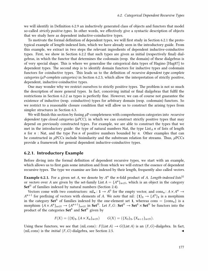
6.2. Categorical Dependent Recursive Types
we will identify in Definition 6.2.9 an inductively generated class of objects and functors that modelso-called strictly positive types. In other words, we effectively give a syntactic description of objectsthat we study here as dependent inductive-coinductive types.
To motivate the formal definition of dependent types, we will first study in Section 6.2.1 the proto-typical example of length-indexed lists, which we have already seen in the introductory guide. Fromthis example, we extract in two steps the relevant ingredients of dependent inductive-coinductivetypes. First, we show in Section 6.2.2 that such types are given as initial (respectively final) dial-gebras, in which the functor that determines the codomain (resp. the domain) of these dialgebras isof very special shape. This is where we generalise the categorical data types of Hagino [Hag87] todependent types. The second step is to identify domain functors for inductive types and codomainfunctors for coinductive types. This leads us to the definition of recursive dependent type completecategories (µP-complete categories) in Section 6.2.3, which allow the interpretation of strictly positive,dependent, inductive-coinductive types.
One may wonder why we restrict ourselves to strictly positive types. The problem is not so muchthe description of more general types. In fact, conceiving initial or final dialgebras that fulfil therestrictions in Section 6.2.2 as types is perfectly fine. However, we can of course not guarantee theexistence of inductive (resp. coinductive) types for arbitrary domain (resp. codomain) functors. Sowe restrict to a reasonable closure condition that will allow us to construct the arising types fromsimpler structures in Section 6.3.
We will finish this section by fusing µP-completeness with comprehension categories into recursivedependent type closed categories (µPCC), in which we can construct strictly positive types that maydepend on previously constructed types. For example, we are able to construct the types that wemet in the introductory guide: the type of natural numbers Nat, the type ListA n of lists of lengthn for n : Nat, and the type Pos n of positive numbers bounded by n. Other examples that canbe constructed in µPCCs include bisimilarity and the substream relation for streams. Thus, µPCCsprovide a framework for general dependent inductive-coinductive types.
6.2.1. Introductory ExampleBefore diving into the formal definition of dependent recursive types, we start with an example,which allows us to first gain some intuition and from which we will extract the essence of dependentrecursive types. The type we examine are lists indexed by their length, frequently also called vectors.
Example 6.2.1. For a given set A, we denote by An the n-fold product of A. Length-indexed lists52
or vectors over A are given by the set-family List A = Ann∈N, which is an object in the categorySetN of families indexed by natural numbers (Section 2.4).
Vectors come with two constructors: nil⋆ : 1 → A0 for the empty vector, and consn : A × An →An+1 for prefixing of vectors with elements of A. We note that nil : 11 → A01 is a morphismin the category Set1 of families indexed by the one-element set 1, whereas cons = consn is amorphism A × Ann∈N → An+1n∈N in SetN. Let F ,G : SetN → Set1 × SetN be functors into theproduct of the categories Set1 and SetN given by
F (X ) = (11, A × Xnn∈N) G(X ) = (X01, Xn+1n∈N).
Using these functors, we see that (nil, cons) : F (List A) → G(List A) is an (F ,G)-dialgebra. In fact,(nil, cons) is the initial (F ,G)-dialgebra, see Section 2.5.
177

Chapter 6. Categorical Logic Based on Inductive-Coinductive Types
At this stage, the reader might be wondering why we are using initial dialgebras rather than initialalgebras to describe the inductive data type in Example 6.2.1. There are two reasons for this. Firstly,as we will see in Definition 6.2.9, using dialgebras allows us to give a straightforward definition of(strictly positive) dependent types. Such a definition is also possible for algebras, cf. Theorem 6.3.1,but much more complicated to carry out. The second reason for using dialgebras is that these allowus the representation of dependent sum and dependent product types as initial and, respectively,final dialgebras. This view will lead to a minimal type theory in Chapter 7.
In Example 6.2.1, we have presented vectors as an initial dialgebra for certain functors. As it turnsout, the functor that describes the codomain of the constructors has a special form.
Example 6.2.2. First, we note that the fibre of Fam(Set) above I is isomorphic to SetI . Let thenz : 1 → N and s : N → N be defined by z(∗) = 0 and s(n) = n + 1, giving us reindexing functorsz∗ : SetN → Set1 and s∗ : SetN → SetN. By their definition, z∗(X ) = X01 and s∗(X ) = Xn+1n∈N,hence the functor G, we used to describe vectors as dialgebra, is G = ⟨z∗, s∗⟩. In Sec. 6.2.2, weaddress the structure of F .
6.2.2. Signatures and Recursive TypesThe idea that underlies the categorical data types of Hagino [Hag87] is that the outcome of aconstructor for a type must be of that type itself. More concretely, a (non-dependent) inductivetype T with n constructors is given by a declaration like that on the left in Figure 6.1. Hagino then
data T wherec1 : F1(T) → T...cn : Fn (T) → T
data Γ ⊢ T’ whereΓ1 ⊢ c ′1 : F ′1(T’) → T’[σ1]...Γ1 ⊢ c ′n : F ′n (T’) → T’[σn]
Figure 6.1.: Declarations of Non-Dependent and Dependent Inductive Types
notices that T corresponds to an initial (F ,G)-dialgebra in a category C with F ,G : C → ∏nk=1 C,
F = ⟨F1, . . . , Fn⟩ and G = ⟨Id, . . . , Id⟩. The dialgebra structure on T is then given by the tuple(c1, . . . , cn), which is a morphism in the category
∏nk=1 C. We now extend this idea to dependent
types. Suppose that T ′ is a dependent type as in Figure 6.1 with variables in context Γ. Eachconstructor c ′k of T ′ may live in a different local context Γk , thus we have to apply a substitutionσk to the type T ′ to bring it into the local context, see the codomain of the constructors c ′k inFigure 6.1. We encountered this already in the example in Section 6.2.1, as the type of vectors overA corresponds to the following type declaration.
data n : Nat ⊢ ListAn where⊢ nil : 1→ ListA 0
k : Nat ⊢ cons : ListAk → ListA (k + 1)
Assume that we are given a fibration P : E → B and that there is an index I ∈ B that correspondsto the context Γ. To view T ′ as an object in the fibre PI , we assume that each Γk corresponds to anobject Jk ∈ B as well. Given this setup, we note that c ′k must be a morphism in PJk , hence F ′k (T
′)
178

6.2. Categorical Dependent Recursive Types
must also be an object in the same fibre. This leads us for each 1 ≤ k ≤ n to the assumption that F ′kis a functor PI → PJk . Similarly, each σk is a substitution that assigns to each variable in the contextΓ a term that lives in context Γk . Therefore, we also assume that there is a morphism uk : Jk → Iin the base B, which in turn gives rise to the reindexing functors u∗k : PI → PJk . These assumptionsallow us to view each constructor c ′k as a morphism F ′k (T
′) → u∗k (T′) in PJk or, equivalently, as
morphism (c ′1, . . . , c′n) in
∏nk=1 PJk . Putting this all together, we will conceive (c ′1, . . . , c
′n) as an
initial dialgebra on T ′ for the functors F ′ and Gu with F ′ = ⟨F ′1, . . . , F ′n⟩ and Gu = ⟨u∗1, . . . ,u∗n⟩. Thisdevelopment is summed in the following definition of a signature and the definition of a recursivetype below in Definition 6.2.7.
Definition 6.2.3. Let P : E→ B be a fibration. A (dependent) recursive-type signature with parametersin a category C, is a pair (F ,u) consisting of
• a functor F : C × PI → D, where D =∏n
k=1 PJk is a product of categories for some n ∈ N,objects Jk ∈ B with k = 1, . . . ,n and I ∈ B, and
• a family u of n morphisms in B with uk : Jk → I for k = 1, . . . ,n.
A family u as above induces a functor Gu : PI → D given by Gu B ⟨u∗1, . . . ,u∗n⟩.
Signatures form the basis of the types we will introduce in Definition 6.2.7. Before we get tothem, let us give the official signature for the type of vectors.
Example 6.2.4. In Example 6.2.2, we have seen that the codomain of the constructors for vectorsare given by a functor G with G = ⟨z∗, s∗⟩. According to Definition 6.2.3, we have G = Gu withu = (z, s), thus the signature of vectors is (F ,u), with the functor F : SetN → Set1 × SetN, as givenin Example 6.2.1.
Note that the parameter category C is trivial (C = 1) in this case. To make the set A, over whichwe considered vectors, a parameter we can use instead the functor F ′ : Set × SetN → Set1 × SetNgiven by F ′(Y ,X ) = (11, Y × Xnn∈N). Note that we then have F ′(A,−) = F for any set A. Thisgives us a signature (F ′,u) with parameters in Set.
We showed in Example 6.2.1 that vectors are an initial (F ,Gu)-dialgebra. This is an instance ofwhat we will call an inductive type for a signature. In Example 6.2.4, we added the set over whichwe consider vectors as a parameter to the signature. So to define types for arbitrary signatures (withparameters), we need to be able to deal with parameterised dialgebras, which are dialgebras thattake further parameters. More technically, these are dialgebras in functor categories for a lifting ofthe functors F and Gu that we will define now. This is analogous to, for example, [Kim10].
Definition 6.2.5. Suppose that we are given a signature (F ,u), where F : C×PI → D. For eachV ∈ Cwe define a functor F (V ,−) : PI → D by putting F (V ,−)(X ) B F (V ,X ). Let us, moreover, assumethat for all V an initial (F (V ,−),Gu)-dialgebra αV : F (V ,ΦV ) → Gu(ΦV ) and final (Gu , F (V ,−))-dialgebra ξV : Gu(ΩV )→ F (V ,ΩV ) exists, where Gu = ⟨u∗1, . . . ,u∗n⟩.
Given these assumptions, we define functors on functor categories with fixed domain C:
F , Gu : [C,PI ]→ [C,D] F (H) B F ⟨IdC,H ⟩ Gu(H) B Gu H . (6.3)
179

Chapter 6. Categorical Logic Based on Inductive-Coinductive Types
We use the dialgebras ΦV and ΦV to build functors µ(F , Gu) : C→ PI and ν(Gu , F ) : C→ PI by
µ(F , Gu)(V ) B ΦV µ(F , Gu)(f : V →W ) B (αW F (f , idΦW ))
ν(Gu , F )(V ) B ΩV ν(Gu , F )(f : V →W ) B (F (f , idΩV ) ξV )∼ ,
where the bar and tilde superscripts denote the inductive and coinductive extensions, that is, theunique homomorphism given by initiality and finality, respectively.
To understand the definition of the functors µ(F , Gu) and ν(Gu , F ), it helps to visualise theirdefinition as homomorphism diagrams:
F (V ,ΘV ) F (V ,ΘW )
F (W ,ΘW )
Gu(ΘV ) Gu(ΘW )
αV
F(V ,µ
(F ,Gu
) )(f )
F(f , idΦW )
αWµ(F ,Gu
)(f )
Gu(ΩV ) Gu(ΩW )
F (V ,ΩV )
F (W ,ΩV ) F (W ,ΩW )
ξV
ν(Gu , F
)(f )
ξW
F(f , idΩV )F(W ,ν
(Gu , F
) )(f )
Now note that F(µ(F , Gu)
)(V ) = F (V ,ΦV ) and Gu
(µ(F , Gu)
)(V ) = Gu(ΦV ), so that the α given in
in Definition 6.2.5 is a family of morphisms, which is moreover natural by uniqueness of inductiveextensions. Since the same also holds for ξ , we obtain the following lemma.
Lemma 6.2.6. The morphisms αV and ξV in Definition 6.2.5 form natural transformations
α : F(µ(F , Gu)
)⇒ Gu
(µ(F , Gu)
)and ξ : Gu
(ν(Gu , F )
)⇒ F
(ν(Gu , F )
). (6.4)
Moreover, α and ξ are, respectively, initial and final dialgebras in the functor category [C,D].
Having set up the notations for parameterised initial and final dialgebras, we can finally definewhat (dependent) recursive types are.
Definition 6.2.7. Let (F ,u) be a recursive-type signature with parameters in C and F : C× PI → D.An inductive type for (F ,u) is an initial (F , Gu)-dialgebra with carrier µ(F , Gu). Dually, a coinductivetype for (F ,u) is a final (Gu , F )-dialgebra, note the order, with the carrier being denoted by ν(Gu , F )Both carriers are functors with
µ(F , Gu) : C→ PI and ν(Gu , F ) : C→ PI .
If C = 1, then we view these carriers as objects in PI and drop the hats from the notation.
We have seen in the introductory guide that dependent coproducts and products play a centralrole in dependent type theory. Moreover, we have claimed that these would arise as inductive andcoinductive types, respectively. The following example makes this statement precise.
180

6.2. Categorical Dependent Recursive Types
Example 6.2.8. Recall from Section 2.4 that a fibration P : E → B is said to have dependentcoproducts and products along a morphism f : I → J in B, if there are functors
⨿f and
∏f from PI
to PJ that are, respectively, left and right adjoint to f ∗. For each X ∈ PI , we can define a signature,such that
⨿f (X ) and
∏f (X ) arise as recursive types for these signatures, as follows. Define the
constant functor by
KX : PJ → PI KX (Y ) = X KX (д) = idX .
With this definition, (KX , f ) is the signature for coproducts and products. For example, the unit ηof the adjunction
⨿f ⊣ f ∗ is the initial (KX , f
∗)-dialgebra ηX : KX (⨿
f (X )) → f ∗(⨿
f (X )), usingthat KX (
⨿f (X )) = X .
To actually get a functor⨿
f : PI → PJ we need to move to a parameterised signature. Theobservation we use is that the projection functor π1 : PI × PJ → PI is a “parameterised” constantfunctor, since we have K J
A = π1(A,−). If we are given f : I → J in B, then we use the signature(π1, f ), and define
⨿f B µ(π1, f ∗) and
∏f B ν( f ∗, π1). We claim now that we indeed get
adjunctions⨿
f ⊣ f ∗ ⊣ ∏f . This will be proven in Thm. 6.2.11. For now, let us just mention that,
for example, the unit η : Id⇒ f ∗⨿
f is given by the initial dialgebra on µ(π1, f ∗).
6.2.3. Recursive-Type Complete Categories
We now define a class of signatures and functors that should be seen as category theoretical lan-guage for, what is usually called, strictly positive types [AM09], positive generalised abstract datatypes [HF11] or descriptions [Cha+10; DM13]. Note, however, that none of these treat coinductivetypes. A non-dependent version of strictly positive types that include coinductive types are givenin [AAG05].
Let us first introduce some notation. Given categories C1 and C2 and an object A ∈ C1, we denoteby KC1
A : C1 → C2 the functor mapping constantly to A. The projections on product categories aredenoted, as usual, by πk : C1 ×C2 → Ck . Using these notations, we can define what we understandto be a recursive type.
Definition 6.2.9. Let P : E → B be a cloven fibration, S a class of signatures in P and D a classof functors. We denote by SC→D ⊆ S the class of all signatures (F ,u) ∈ S such that F : C → D.Similarly, DC→D ⊆ D is the class of all functors F ∈ D with F : C→ D.
We say that P is a recursive-type complete category (µP-complete category) if there is a class S ofsignatures in P and a class D of functors subject to the following closure rules. The class S mustbe closed under formation of signatures over D with arbitrary reindexing morphisms in B:
D =∏n
i=1 PJi F ∈ DC×PI→D u = (u1 : J1 → I , . . . ,un : Jn → I) morphisms in B(F ,u) ∈ SC×PI→D
The classD must contain base types and must be closed under pairing, composition and the formation
181

Chapter 6. Categorical Logic Based on Inductive-Coinductive Types
of recursive types from signatures in S:
A ∈ PJKPIA ∈ DPI→PJ
C =∏n
i=1 PIiπk ∈ DC→PIk
f : J → I in Bf ∗ ∈ DPI→PJ
F1 ∈ DPI→PK F2 ∈ DPK→PJF2 F1 ∈ DPI→PJ
Fi ∈ DPI→PJi i = 1, 2
⟨F1, F2⟩ ∈ DPI→PJ1×PJ2
(F ,u) ∈ SC×PI→D
µ(F , Gu) ∈ DC→PI
(F ,u) ∈ SC×PI→D
ν(Gu , F ) ∈ DC→PI
If S and D are the minimal classes that are closed under these rules, then we call S the class ofstrictly positive signatures and D the class of strictly positive types.
A brief note about terminology: The name µP-complete is an adaption of the λ-cube terminology,where the calculus with just dependent types is called λP, see [Bar91; NG14]. The letter “P” stands inthis context for “predicate” and signifies the involvement of dependent types. With the Greek letterµ, we intend to refer to recursive types and not just inductive types. The reader should think hereof general µ-recursion as a mnemonic, similar to the naming of µ-bicomplete categories [San02b].
The following assumption reflects that D contains exactly the strictly positive types we willconsider in Chapter 7.
Assumption 6.2.10. We assume, without loss of generality, that for a µP-complete category, theclasses S and D are exactly its strictly positive signatures and types.
One feature of recursive-type complete categories is that basic types, like fibrewise and dependentproducts and coproducts, arise naturally as inductive and coinductive types. This is an instance ofthe following, more general, result.
Theorem 6.2.11. Suppose P : E→ B is a µP-complete category. LetC =∏n
i=1 PJi and π1 : C×PI → Cbe the first projection. If (π1,u) is a signature such uk : Ji → I , then we have for Gu = ⟨u∗1, . . . ,u∗n⟩ thefollowing adjoint situation:
µ(π1, Gu) ⊣ Gu ⊣ ν(Gu , π1).
Proof. We only show how the adjoint transposes are obtained in the case of inductive types. Con-cretely, for a tuple V ∈ C and an object A ∈ PI , we need to prove the correspondence
f : µ(π1, Gu)(V ) −→ A in PI
д : V −→ GuA in C
Let us use the notation H = µ(π1, Gu), then the choice of π1 implies that the initial (π1, Gu)-dialgebrais of type α : IdC ⇒ Gu H , since π1(H) = π1 ⟨IdC,H ⟩ = IdC and Gu(H) = Gu H . This allows usto use as transpose of f the morphism V
αV−−→ Gu(H(V ))Gu f−−−→ GuA. As transpose of д, we use the
inductive extension of π1(KCA)(V ) = V
д−→ GuA = Gu(K
CA)(V ). The proof that this correspondence
is natural and bijective follows straightforwardly from initiality. For coinductive types, the result isgiven by duality.
182

6.2. Categorical Dependent Recursive Types
From this result we can recover the usual binary, fibrewise products and coproducts, and thedependent products and coproducts as shown in the following table.
Construction Parameter C Reindexing u DefinitionBinary Coproduct +I : PI × PI → PI PI (idI , idI ) +I = µ(π1, Gu)
Binary Product ×I : PI × PI → PI PI (idI , idI ) ×I = ν(Gu , π1)
Dependent Coproduct⨿
f : PI → PJ 1 (f : I → J)⨿
f = µ(π1, Gu)
Dependent Product⨿
f : PI → PJ 1 (f : I → J)∏
f = ν(Gu , π1)
Many more examples, like initial and final objects etc., can be obtained in a µP-complete category,but we defer their construction to the examples in Chapter 7 to reduce repetition. Let us give twoexamples that become relevant in Section 6.4 though.
Example 6.2.12 (Propositional Equality). There are several definable notions of equality, providedthat B has binary products. A generic one is propositional equality EqI : PI → PI×I , the left adjointto the so-called contraction functor δ ∗ : PI×I → PI , where δ is the diagonal δ : I → I × I . Thus,propositional equality can be obtained from the table above as the dependent coproduct along δ :EqI B
⨿δ . Since EqI is a left adjoint, it comes for each X ∈ PI×I with a constructor reflX : X →
δ ∗(EqI (X )).Let us clarify this definition by instantiating it over set families. For Y ∈ SetI×I and i ∈ I , we
have δ ∗(Y )i = Yδ (i) = Y(i,i). The equality type on X ∈ SetI and (i, j) ∈ I × I is given on the otherhand by
EqI (X )(i, j) =⨿k ∈I
δ (k)=(i, j)
Xk
Xi , i = j
∅, i , j.
The constructor reflX is given for each i ∈ I as a map Xi → EqI (X )(i,i) Xi , and is essentially theidentity map. It should be noted that one is usually more interested in the instance EqI (1I ), where1I in the final object in PI . For this reason, we define
Eq(I) B EqI (1I ). (6.5)
In Fam(Set), one obtains thus
Eq(I) = EqI (1I ) 1, i = j
∅, i , j,
which is the definition of equality on I that might be more familiar.
Example 6.2.13 (Bisimilarity for Streams). Assume that there is an object Aω in B of streams overA, together with projections hd : Aω → A and tl : Aω → Aω , giving us the head and tail of a stream.We can define bisimilarity between streams as coinductive type for the signature
F ,Gu : PAω×Aω → PAω×Aω × PAω×AωF =
⟨(hd × hd)∗ KEq(A), (tl × tl)∗
⟩and u = (idAω×Aω , idAω×Aω ).
183

Chapter 6. Categorical Logic Based on Inductive-Coinductive Types
Let us put this definition of bisimilarity into a broader perspective. There is a category Rel(E) ofbinary relations in E by forming the pullback of P along ∆: B→ B with ∆(I) = I × I , see [HJ97]:
Rel(E) E
B B
Rel(P) P
∆
Since P is cloven, also the resulting fibration Rel(P) is cloven ([Jac99, Lem. 1.5.1]). Thus, we obtainreindexing functors between the fibres of Rel(E), which we will denote by (−)#. Note that the fibresof Rel(E) can be presented by the isomorphism Rel(E)X PX×X , so that reindexing in Rel(P) iseffectively given by f # = (f × f )∗. We can now reinterpret F and Gu in Rel(E) by
F ,Gu : Rel(E)Aω → Rel(E)Aω × Rel(E)AωF = ⟨hd# KEq(A), tl#⟩ and Gu = ⟨id#
Aω , id#Aω ⟩.
The final (Gu , F )-dialgebra on BisimA ∈ Rel(E)Aω is a pair of morphisms(hd∼A : BisimA → hd#(Eq(A)), tl∼A : BisimA → tl#(BisimA)
).
BisimA should be thought of to consist of all bisimilarity proofs. Coinductive extensions yield theusual coinduction proof principle, allowing us to prove bisimilarity by establishing a bisimulationrelation R ∈ Rel(E)Aω together with h : R → hd#(Eq(A)) and t : R → tl#(R). This says, as usual, thatthe heads of streams related by R are equal and that the tails of related streams are again related.Later, in Example 6.4.13, we will see how bisimilarity arises canonically for coinductive types.
Let us now come to an example of a truly dependent, inductive-coinductive type. This type willrepresent the substream relation that we encountered before.
Example 6.2.14. Recall that we have defined in Example 5.1.13 the substream relation that relatestwo streams s and t , if all the elements in s occur in order in t . We denoted this relation symbolicallyby s ≤ t . In Section 5.1.3, we found out that this relation could be expressed by selecting elementsfrom the stream t through an inductive-coinductive type. From this, we inferred that ≤ is aninductive-coinductive relation. The purpose of this example is to make this somewhat more preciseby defining ≤ directly as a recursive type. In Section 7.5.3 we will relate both definitions.
To give an intuitive description of the direct definition of the substream relation, let us use for amoment the language of the copattern calculus λµν=. Let s and t thus be of type Aω . We considers to be substream of t , written s ≤ t , if we can obtain a stream t ′ by finitely often applying .tl to t ,such that
1. s .hd = t ′.hd, and
2. s .tl ≤ t ′.tl.
Figure 6.2 should give an idea of how this definition works for streams of natural numbers.Let us now derive from this description a definition of the substream relation in a µP-complete
category. As a first towards this goal consider the following mutually recursive declaration of thedependent types s ≤ t and s ≤µ t .
184

6.2. Categorical Dependent Recursive Types
t : 1 5 0 3 1 2 4 · · ·
s: 0 1 2 3 4 5 6 · · ·
t ′ = t .tl.tl
s .tlFigure 6.2.: Operational View on Substream Relation
codata s, t : Aω ⊢ s ≤ t whereout : s ≤ t → s ≤µ t
data s, t : Aω ⊢ s ≤µ t wherematch : (s.hd = t.hd) × (s.tl ≤ t.tl) → s ≤µ tskip : s ≤µ t.tl → s ≤µ t
The first type is coinductive, which is signified by the keyword codata, whereas the second is aninductive type. Of course, the first type should represent the substream relation. But what is therole of the type s ≤µ t? Note that in the description of the substream relation above we said that fors ≤ t to hold there must be a stream t ′ that is obtained by finitely often applying the tail destructorto t . These skipping steps can be exactly achieved by using the “skip” constructor of s ≤µ t and,since this is an inductive type, we eventually need to use the “match” constructor. This constructor,in turn, requires us to show that the heads of s and t match and that the tail of s is a substream ofthe tail of t ′. Hence, “match” formalises exactly the two conditions we posed above on t ′.
In Figure 6.3, we give a representation of a proof tree for the fact that the constant stream 1ω isa substream of the alternating bit stream alt. Since the tail of alt starts with a 1, we use for claritythe notation 1 : alt instead of alt.tl in the tree. Moreover, the dashed line shows how the proof treeis build through the coinductive type 1ω ≤ alt. We will give a formal definition of this proof byusing finality of the substream relation.
skip(1ω ,alt)
match(1ω ,1 : alt)refl1
Figure 6.3.: Conceptual Representation of a Proof of 1ω ≤ alt
After developing an intuition for how the substream relation arises as an inductive-coinductivetype, it is now our job to construct this relation by using the machinery of µP-complete categories.This is done in three steps: First, we define a functor S ′µ : Rel(E)Aω → Rel(E)Aω , such that S ′µ (R)corresponds to ≤µ but with all occurrences of ≤ in its declaration replaced by R. Second, we defineS ∈ Rel(E)Aω , which corresponds to ≤. Finally, the type ≤µ itself is interpreted as S ′µ (S). SinceS ′µ : Rel(E)Aω → Rel(E)Aω should be an inductive type, we define S ′µ = µ
(F , Gu
)with
F : Rel(E)Aω × Rel(E)Aω → Rel(E)Aω × Rel(E)AωF (S,R) =
(hd#(Eq(A)) × tl#(S), (id × tl)∗(R)
)185

Chapter 6. Categorical Logic Based on Inductive-Coinductive Types
and u = (idAω , idAω ). On top of this type, we can now define the substream relation S ∈ Rel(E)Aωby S = ν
(GidAω , S
′µ). Notice how these definitions reflect exactly the type declarations above because
with Sµ = S ′µ (S) we obtain the following operations, since S and Sµ are final and initial dialgebras.
out : S → Sµ
match : hd#(Eq(A)) × tl#(S)→ Sµ
skip : (id × tl)∗(Sµ )→ Sµ
Coming back to the example that 1ω is a substream of alt, we can give in Rel(Fam(Set))Aω aformal description of the proof tree in Figure 6.3. To do so, recall that Rel(Fam(Set))Aω SetAω×Aω ,which allows us to define relations easily as set families. Thus, let us define R ∈ SetAω×Aω to be
R(σ ,τ ) =
1, σ = 1ω and τ = alt∅, otherwise
.
We can then define morphism c : R → S ′µ (R) in SetAω×Aω by
c(1ω ,alt)(⋆) = skip(1ω ,alt)(match(1ω ,1 : alt)(refl1(⋆),⋆)
).
Since id#(R) Id(R) = R, we have that c is a(Gid, S
′µ)-dialgebra and can thus be extended to a
homomorphism c : R → S . By applying this map, we obtain the tree in Figure 6.3 as the elementc(1ω ,alt)(⋆) in S .
Summing up, we have shown how to construct the substream relation in any µP-complete category.We show that this direct definition is equivalent to the one given by stream filtering in Section 5.1.3.
Up to this point, all coinductive types that we encountered only used the identity substitution todetermine the domain of their destructors. In the last example of this section we study a dependentcoinductive type that uses a non-trivial substitution instead. The point of this example is to illustratehow non-trivial substitutions allow us to block the application of destructors.53 54
Example 6.2.15. A partial stream is a stream together with a, possibly infinite, depth up to whichit is defined. Assume that there is an object N∞ of natural numbers extended with infinity and asuccessor map s∞ : N∞ → N∞ in B, we will see how these can be defined in Example 6.2.19. Thepartial streams correspond to the following type declaration, the idea of which is that the head andtail of partial streams are defined only on those partial streams that are defined in, at least, the firstposition.codata n : N∞ ⊢ PStr A n where
k : N∞ ⊢ hd k : PStr A (s∞ k) → Ak : N∞ ⊢ tl k : PStr A (s∞ k) → PStr A k
As set of partial functions, we can define partial streams as a family indexed by n ∈ N∞:
PStr(A)n = s : N A | ∀k < n.k ∈ dom s ∧ ∀k ≥ n.k < dom s,
where the order on N∞ is given by extending that of the natural numbers with ∞ as strict topelement, that is, such that k < ∞ for all k ∈ N.
186

6.2. Categorical Dependent Recursive Types
The interpretation of PStr(A) for A ∈ P1 in a µP-complete category is given as the carrier of thefinal (Gu , F )-dialgebra with
Gu , F : PN∞ → PN∞ × PN∞ Gu =⟨s∗∞, s
∗∞⟩
F =⟨KN
∞A′ , Id
⟩,
where A′ = !∗N∞(A) ∈ PN∞ is the weakening of A with !N∞ : N∞ → 1. On set families, partial streams
are given by the dialgebra ξ = (hd, tl)with hdk : PStr(A)(s∞ k) → A and tlk : PStr(A)(s∞ k) → PStr(A)kfor every k ∈ N∞.
We can make this construction functorial in A, using the same “trick” as for sums and products.To this end, we define the functor H : P1 × PN∞ → PN∞ × PN∞ with H =
⟨!∗N∞ π1,π2
⟩, where π1
and π2 are corresponding projection functors, so that H(A,X ) = F (X ). This gives, by recursive-typecompleteness, rise to a functor ν(Gu , F ) : PN∞ → PN∞ , which we denote by PStr, together with apair (hd, tl) of natural transformations.
6.2.4. Recursive-Type Closed Categories
We have seen in the introduction that one of central notions in a (dependent) type theory is contextextension. It turned out that a possible category theoretical counterpart was to have a comprehensionfunctor. The following definition gives a precise description of the necessary ingredients that afibration with comprehension needs to have, so that dependently typed contexts can be interpretedover that fibration. This definition can be found, for example, in [Jac99, Lem. 1.8.8, Def. 10.4.7]and [FGJ11].
Definition 6.2.16. Let P : E → B be a fibration. If each fibre PI has a final object 1I and theseare preserved by reindexing, then there is a fibred final object functor 1(−) : B→ E. (Note that thenP(1I ) = I .) P is a comprehension category with unit (CCU ), if 1(−) has a right adjoint − : E → B,called comprehension. This gives rise to a functor P : E → B→ into the arrow category over B, bymapping P(A) = P(εA) : A → P(A) and P(f ) = ( f , P f ), where ε : 1− ⇒ Id is the counit of1(−) ⊣ −. We often denote P(A) by πA and call it the projection of A. Finally, P is said to be a fullCCU , if P is a fully faithful functor.
Note that, in a µP-complete category, we can define final objects in each fibre, though the preser-vation of them by reindexing needs to be required separately, see Section 6.5.
Let us record for later use what the fullness conditions for a CCU means explicitly. Recall thata morphism between projections πA and πB in the arrow category B→ is given by a commutingdiagram of the following form.
A B
PA PB
f
πA πBд
That P is a fully faithful functor means now that there is a unique h : A→ B in E with P(h) = (f ,д).By definition of P, we thus have f = h and д = Ph.
The following example describes comprehension for the set-family fibration, which he have en-countered already in the introduction.
187

Chapter 6. Categorical Logic Based on Inductive-Coinductive Types
Example 6.2.17. In Fam(Set), the final object functor is given by 1I = (I , 1i ∈I ), where 1 is thesingleton set. Comprehension is defined to be (I ,X ) = ⨿
i ∈I Xi and the projections πI map thenan element of
⨿i ∈I Xi to its component i in I .
Using comprehension, we can give a general account to dependent recursive types.
Definition 6.2.18. We say that a fibration P : E→ B is a recursive-type closed category (µPCC), if itis a CCU, has a terminal object in B and is µP-complete.
As already mentioned, the purpose of introducing comprehension is that it allows us to userecursive types defined in E again as index. The terminal object in B is used to introduce recursivetypes without dependencies, like natural numbers. Let us reiterate on Ex. 6.2.15 to illustrate this.
Example 6.2.19. Recall that we assumed the existence of extended naturals N∞ and the successormap s∞ on them to define partial streams. We are now in the position to define in a recursive-typeclosed category everything from scratch as follows.
Having defined + : P1 × P1 → P1, see Thm. 6.2.11, we put N∞ B ν(Id, 1 + Id) with its finaldialgebra structure being the predecessor pred. The successor map s∞ : N∞ → N∞ can then bedefined as the unique homomorphism in the following diagram.
N∞ N∞
1+ N∞ N∞
s∞
κ2 predid+s∞
Partial streams PStr : PN∞ → PN∞ are then given as in Ex. 6.2.15 by the final (Gu , F )-dialgebra,only this time we need to apply the comprehension functor to s∞ to obtain a map in the basecategory B. Thus, we put u = (s∞, s∞) and F =
⟨!∗N∞ π1,π2
⟩.
6.3. Constructing Recursive Types as PolynomialsIn Section 6.2, we have given conditions on fibrations that allow us to use them as dependenttype theory based only on inductive and coinductive types. The important notion there was thatof µP-completeness (Definition 6.2.9). This raises of course the question whether there are anyexamples of µP-complete categories. We will answer this question affirmatively by showing thatthere is a class of categories, called Martin-Löf categories, that admit an interpretation of all necessaryrecursive types. This works by reducing all recursive types to polynomial functors [GK13] (also calledcontainer [AAG05]). An example of this class is then the codomain fibration over the category ofsets.
The construction proceeds in two steps. First, we reduce in Theorem 6.3.1 the dialgebras arisingfrom signatures to algebras and coalgebras, respectively. Second, we construct the necessary initialalgebras and final coalgebras as fixed points of polynomial functors, analogous to the constructionof strictly positive types in [AAG05]. This second step is again an assembly of results. We provein Theorem 6.3.10 that fixed points of dependent polynomial functors with parameters are againpolynomial functors. This allows us to construct nested recursive types, and is the significant result ofthis section. Next, we show that dependent recursive types can be constructed from non-dependent
188

6.3. Constructing Recursive Types as Polynomials
recursive types. For coinductive types the corresponding result is given in Theorem 6.3.6, whereasthe analogous result for inductive types is already in [AAG05] and [GK13]. Finally, the constructionof non-dependent, coinductive types can be reduced to that of inductive types, which is again provedby Abbott et al. [AAG05].
We begin by showing that inductive and coinductive types correspond to certain initial algebrasand final coalgebras, respectively.
Theorem 6.3.1. Let P : E → B be a fibration with fibrewise coproducts and dependent sums. If (F ,u)with F : PI → PJ1 × · · · × PJn is a signature, then there is an isomorphism
DiAlg(F ,Gu) Alg(⨿u1
F1 +I · · ·+I
⨿un
Fn)
where Fk = πk F is the kth component of F . In particular, existence of inductive types and initial algebrascoincide. Dually, if P has fibrewise and dependent products, then
DiAlg(Gu , F ) CoAlg(∏u1
F1 ×I · · · ×I∏un
Fn).
In particular, existence of coinductive types and final coalgebras coincide.
Proof. The first result is given by a simple application of the adjunctions⨿n
k=1 ⊣ ∆n between the(fibrewise) coproduct and the diagonal, and
⨿uk ⊣ u∗k :
FX −→ GuX (in PJ1 × · · · × PJn )
(⨿
u1(F1X ), . . . ,
⨿un (FnX )) −→ ∆nX (in PnI )⨿n
k=1
⨿uk (FkX ) −→ X (in PI )
That homomorphisms are preserved follows at once from naturality of the used Hom-set isomorph-isms. The correspondence for coinductive types follows by duality.
To be able to reuse existing work, we work in the following with the codomain fibrationcod : B→ → B for a category B with pullbacks. Moreover, we assume that B is finitely com-plete and locally Cartesian closed. The following definition allows to connect this to our setup offibrations.
Definition 6.3.2 ([Jac99, Def. 10.5.3]). Let P : E→ B be a comprehension category with coproducts,that is, for every A ∈ E with projection πA : A → PA there is an adjunction
⨿A ⊣ π ∗A that
satisfies the Beck-Chevalley condition, see Definition 2.4.4. We denote the unit of these coproductsby η : Id⇒ π ∗A
⨿A, and we let πA (
⨿A X ) be the Cartesian lifting of πA as in the following diagram.
π ∗A⨿
A X⨿
A X
A PA = P(⨿
A X )
πA (⨿
A X )
πA
P
189

Chapter 6. Categorical Logic Based on Inductive-Coinductive Types
The fibration P has strong coproducts, if the dependent pairing κ : X → ⨿I X , given by
κ =πA
(⨿AX
) ηX
,
is an isomorphism. We call P a closed comprehension category (CCompC), if it is a full CCU withproducts, strong coproducts and has a final object in the base category B.
By [Jac99, Thm 10.5.5], a finitely complete category B is locally Cartesian closed if and only ifthe codomain fibration is cod : B→ → B is a closed comprehension category. Another assumptionthat we need is that the binary coproducts in B are disjoint, which means that the injections aremonomorphisms and form the following pullback square.
0 J
I I + J
κ2κ1
Under the assumption that coproducts are disjoint, we obtain an equivalence B/I+J ≃ B/I × B/J ,see [Jac99, Prop. 1.5.4].
Assumption 6.3.3. In this section we assume that B is a finitely complete, locally Cartesian closedcategory with disjoint coproducts.
Definition 6.3.4. A dependent polynomial Γ indexed by I on variables indexed by J is given by atriple of morphisms
B A
J Is
ft
If J = I = 1, f is said to be a (non-dependent) polynomial. The extension of a polynomial Γ is givenby the composite JΓK = B/J s∗−→ B/B
∏f−−→ B/A
⨿t−−→ B/I ,
which we denote by Jf K if Γ is non-dependent. A functor F : B/J → B/I is a dependent polynomialfunctor , if there is a dependent polynomial Γ such that F JΓK.
Note that polynomials are called containers by Abbott et al. [Abb03; AAG05], and a polynomialΓ = 1
!←− Bf−→ A
!−→ 1 would be written as A ▷ f there. Similarly, dependent polynomials are a slightgeneralisation of indexed containers [AM09]. Container morphisms, however, are different fromthose of dependent polynomials, as the latter correspond to strong natural transformations [GK13,Prop. 2.9], whereas the former are in exact correspondence with all natural transformations betweenextensions [AAG05, Thm. 3.4]. Because of this relation, we will apply results for containers, whichdo not involve morphisms, to polynomials. Another difference in terminology between the theory ofpolynomial functors and containers is that initial algebras and final coalgebras for functors associatedto containers are called and W-types and M-types, respectively. We will adopt this terminology inthe following and denote for f : A→ B byWf the carrier of the initial algebra and by Mf the carrierof the final coalgebra for Jf K. In particular, we can use this to translate [AAG05, Prop. 4.1], givingus a construction of final coalgebras for polynomial functors from initial algebras for polynomialfunctors.
190

6.3. Constructing Recursive Types as Polynomials
Assumption 6.3.5. We assume additionally that B is closed under the formation of W-types, thusis a Martin-Löf category in the terminology of Abbott et al. [AAG05]. By the above remark, B thenalso has all M-types.
Analogously to how [GH04, Thm. 12] extends [MP00, Prop. 3.8], we extend here [vdBdM04,Thm 3.3]. That is to say, we show that final coalgebras for dependent polynomial functors can beconstructed from final coalgebras of non-dependent polynomial functors. One reviewer of [Bas15a]had pointed out that this result can be derived from [vdBdM07, Thm 3.1], the published versionof [vdBdM04]. However, we include a proof here, since it gives some insight into the handling ofdependencies.
Theorem 6.3.6. Dependent polynomial functors B/I → B/I have final coalgebras.
Proof. Let Γ = Is←− B
f−→ A
t−→ I be a dependent polynomial. We construct, analogously to [GH04],the carrier of a final coalgebra V of JΓK as an equaliser as in the following diagram, in which f × Iis a shorthand for B × I
f ×idI−−−−→ A × I and Mf ×I is the carrier of the final Jf × IK-coalgebra.V Mf Mf ×I
д u1
u2
(6.6)
First, we give u1 and u2, whose definitions are summarised in the following two diagrams.
Mf Mf ×I
Jf K(Mf )
Jf × IK(Mf ) Jf × IK(Mf ×I )
u1
ξf
ξf ×I
pMf Jf ×IK(u1)
Mf Mf ×I Mf ×I
Jf × IK(Mf ×I )
Jf × IK(Mf ×I × B) Jf × IK(Mf ×I )
u1
u2
ξf ×I
ψ
ξf ×I
ΣA×IK Jf ×IK(φ)These diagrams shall indicate that u1 is given as coinductive extension and ψ as one-step definition,using that Mf ×I is a final coalgebra, see Appendix B. The maps involved in the diagram are givenas follows, which we sometimes spell out in the internal language of the codomain fibration, see forexample [Abb03], as this is sometimes more readable.55
• The natural transformation p : ΣAΠf ⇒ ΣA×IΠf ×I sends (a,v) to (a, t(a),v). It is given bythe extension Jα , βK : Jf K⇒ Jf × IK of the morphism of polynomials [AAG05]
B A
B × I A × I
f
β αf ×I
where α = ⟨id, t⟩ and β = ⟨id, t f ⟩.
191

Chapter 6. Categorical Logic Based on Inductive-Coinductive Types
• The map K : Πf ×I (Mf ×I )→ Πf ×I (Mf ×I × B) is given as transpose of
⟨εMf ×I ,π1 π ⟩ : (f × I)∗(Πf ×I (Mf ×I ))→ Mf ×I × B,
where ε is the counit of the product (evaluation) and π is the context projection. In theinternal language K is given by K v = λ(b, i).(v (b, i),b).
• φ : Mf ×I × B → Mf ×I is constructed as coinductive extension as in the following diagram
Mf ×I × B Mf ×I
Jf × IK(Mf ×I ) × B
Jf × IK(Mf ×I × B) Jf × IK(Mf ×I )
ξf ×I×id
φ
ξf ×I
e Jf ×IK(φ)Here e is given by e((a, i,v),b) = (a, s b, λ(b ′, s b).(v (b ′, i),b ′)), arising from the so-calledFrobenius property, see [Jac99, Lem. 1.9.12].
We note that the elements of the subobject V of Mf , as given in (6.6), can be described by
x : Vi ⇐⇒ξf x = (a : A,v : Πf Mf ), t a = i and (∀b : B. f b = a ⇒ v b : Vs b).
The direction from left to right is given by simple a calculation, whereas the other direction can beproved by establishing a bisimulation between u1 x and u2 x . We defer these details to Appendix B.
This characterisation of V allows us to prove that ξf : Mf → Jf K(Mf ) restricts to ξ ′ : V → JΓK(V )and that ξ ′ is a final coalgebra. Hence, V is indeed the carrier of a final JΓK-coalgebra in B/I .
Before we continue, let us briefly illustrate the construction of final coalgebras for dependentpolynomials from non-dependent polynomials in Set→.
Example 6.3.7. Recall from Ex. 6.2.15 that partial streams are given bycodata n : N∞ ⊢ PStr A n where
k : N∞ ⊢ hd k : PStr A (s∞ k) → Ak : N∞ ⊢ tl k : PStr A (s∞ k) → PStr A k
and that PStr is the final (Gu , H)-dialgebra, where we have that H : Set1 × SetN∞ → SetN∞ × SetN∞
with H =⟨!∗N∞ π1,π2
⟩and u = (s∞, s∞). By Thm. 6.3.1, we can construct PStr as the final coalgebra
of F : Set/1 × Set/N∞ → Set/N∞ with F (A,X ) =∏
s∞ !∗N∞ A ×N∞
∏s∞ X .
Let us now fix an object A ∈ Set/1 and put A′ B !∗N∞(A). To represent F (A,−) as a polynomialfunctor, we will need the following pullback
Q⨿N∞
∏s∞ A
′
N∞ N∞
p
f
π
s∞
(6.7)
192

6.3. Constructing Recursive Types as Polynomials
(3,a0)
(∞,a1)
(15,a2)
...
(2, 3, a0)
(∞, ∞, a1)
(14, 15, a2)
f (3,b0)
(2,b1)
(1,b2)
(0,⊥)
(2, 3, b0)
(1, 2, b1)
(0, 1, b2)
3 π
2
p
π
1
p
π
0
p
π
(∞, c0)
(∞, c1)
(∞, c2)
...
(∞, ∞, c0)
(∞, ∞, c1)
(∞, ∞, c2)
∞ π
Figure 6.4.: Intermediate trees constructed in Thm. 6.3.6; only the last two are valid
where π is the evident coproduct projection. Now we have
F (A,X ) =∏
s∞A′ ×N∞
∏s∞
X
⨿
ππ ∗
(∏s∞
X)
× represented by⨿
⨿
π
∏fp∗X Beck-Chevalley with (6.7)
= JΓK(X ),
where Γ is the polynomial given by
Γ = N∞p←− Q
f−→
⨿N∞
∏s∞
A′π−→ N∞.
To be able to picture trees in Mf and in the final coalgebra of JΓK, we note that
Q (k, (n,v)) ∈ N∞ ×
⨿N∞
∏s∞
A′ s∞k = n
.
Moreover, we denote a pair (n,v) ∈ ⨿N∞
∏s∞ A
′ by (n,a) if there in a k ∈ N∞ with n = s∞ k andv k = a, or if n = 0 by (0,⊥).
Recall that we construct in Thm. 6.3.6 the final coalgebra of JΓK as a subobject of Mf . In Figure 6.4,we present three trees that are elements of Mf , where only the second and third are actually selectedby the equaliser taken in Thm. 6.3.6. The matching of indices, which is used to form the equaliser,is indicated in the second tree. This tree is then an element of PStr(A)3, whereas the third is inPStr(A)∞.
Both in [AAG05, Prop. 4.1] and [vdBdM07, Cor. 4.3] it is shown that a final coalgebra for apolynomial functor can be constructed in a Martin-Löf category from an initial algebra and anequaliser. This is closely related the result of Barr [Bar93], which states that a final coalgebra of an(accessible, ω-continuous) functor F with F∅ , ∅ is the Cauchy completion of its initial algebra. Wecan combine this with Theorem 6.3.6 to obtain final coalgebras for dependent polynomial functorsfrom initial algebras of (non-dependent) polynomial functors. This gives us already the possibility
193

Chapter 6. Categorical Logic Based on Inductive-Coinductive Types
of interpreting non-nested fixed points in any Martin-Löf category. So it remains to show that wecan interpret nested fixed points.
We proceed as follows. Suppose that we are given a parameterised signature (F ,u) with F : C ×B/I → D, C =
∏mi=1 B/Ki , D =
∏ni=1 B/Ji , and ui : Ji → I . Then we need to show that µ(F , Gu)
and ν(F , Gu) are both polynomial functors of type C→ B/I . To do so, we first use Thm. 6.3.1, thuswe have to show that for each A ∈ C the intial algebra respectively final coalgebra of the functors
H1(A,−) =⨿u1
F1(A,−) +I · · ·+I
⨿un
Fn(A,−)
H2(A,−) =∏u1
F1(A,−) ×I · · · ×I∏un
Fn(A,−)
give rise to polynomial functors, assuming that F1, . . . , Fn are polynomial functors. Let K be givenby K = K1 + · · · + Kn , then one can use the equivalence C × B/I ≃ B/K+I to show that there arepolynomial functors H ′k : B/K+I → B/I that are naturally isomorphic to C × B/I ≃ B/K+I
Hk−−→ B/I ,see [Abb03, Prop. 4.4.2]. Such functors H ′k are captured by the following definition.
Definition 6.3.8. We call a dependent polynomial parametric, if it is of the form
K + I B A I .s f t
As we have seen, such polynomials represent polynomial functors B/K × B/I → B/I and allowus speak about nested fixed points. What thus remains is that fixed points of parametric dependentpolynomial functors are again dependent polynomial functors. Towards this, we first bring parametricpolynomials into a convenient form.
Lemma 6.3.9. Let
Γ : K + I B A I ,s f t
be a parametric polynomial. Then there are two polynomials
K B1
A I
I B2
s1f1
t
s2f2
such that for all Z ∈ B/K+I ⨿t
(∏f1s∗1 κ
∗1 Z ×A
∏f2s∗2 κ
∗2 Z
) JΓK(Z),
where κ1 : K → K + I and κ2 : I → K + I .
Proof. We form the pullbacks
B1 K
B K + I
s1
p1 κ1
s
B2 I
B K + I
s2
p2 κ2
s
194

6.3. Constructing Recursive Types as Polynomials
and put fi = f pi . Then, using the abbreviations X = κ∗1 Z and Y = κ∗2 Z , we have⨿t
(∏f1s∗1X ×A
∏f2s∗2 Y
)
⨿t
(∏f
∏p1s∗1X ×A
∏f
∏p2s∗2 Y
) ∏f pi
∏f
∏pi
⨿
t
(∏fs∗
∏κ1
X ×A∏
fs∗
∏κ2Y)
Beck-Chevalley
⨿
t
∏fs∗
(∏κ1
X ×K+I
∏κ2Y)
fibred product
⨿
t
∏fs∗
(∏κ1κ∗1 Z ×K+I
∏κ2κ∗2 Z
)Def. X ,Y
⨿
t
∏fs∗ Z Disjoint coprod.
= JFK(Z)
We are now in the position to prove that initial algebras and final coalgebras of parametricpolynomial functors are again polynomial functors, the final step towards constructing recursivetypes. The proof of this fact follows that for container [Abb03, Sec. 5.3-5.5] or for non-dependentpolynomials [GH04], except that we need to take care of the indices.
Theorem 6.3.10. Initial algebras and final coalgebras of parametric (dependent) polynomial functorsare again polynomial functors. More formally, let F : B/K+I → B/I be a parametric polynomial functor.Then there are polynomial functors µF ,νF : B/K → B/I and natural transformations
α : F (µF )⇒ µF and ξ : νF ⇒ F (νF ),
so that α is an initial algebra and ξ a final coalgebra for F : [B/K,B/I ]→ [B/K,B/I ].
Proof. Suppose F is given by the parametric polynomial
Γ : K + I B A I .s f t
Then, by Lemma 6.3.9, we obtain two polynomials
Γ1 : K B1
A I
Γ2 : I B2
s1f1
t
s2f2
that represent JΓK. Let H : B/K × B/I → B/I be the functor given by
H(X ,Y ) B⨿
t
(∏f1s∗1X ×A
∏f2s∗2 Y
). (6.8)
The goal is then to show that there is a polynomial functor G : B/K → B/I that carries the structureof an initial algebra or final coalgebra, respectively.
195

Chapter 6. Categorical Logic Based on Inductive-Coinductive Types
As a first step, let us assume that such a G exists and is given by G J∆K with
∆ : K Q P I .x h y
Then we must have for each X ∈ B/K an isomorphism H(X ,G(X )) G(X ). We now want tocalculate, as in [Abb03, Sec. 5.3-5.4], how ∆ needs to be given.
The first step is to define y : P → I , an easy calculation shows that there must be an isomorphism
ψ : JΓ2K(y) −→ y. (6.9)
So, analogously to [Abb03; GH04], we construct y as the carrier of an initial algebra or final coalgebra,respectively, of JΓ2K, depending on whether G should be the carrier of an initial algebra or finalcoalgebra.
To define h and x , we first introduce a few morphisms obtained from pullbacks. Their purposewill become clear once we give the constraints introduced by the isomorphism H(X ,G(X )) G(X ).First, we reindex y along s2 by means of the following pullback.
s∗2 P P
B2 I
s∗2 y
s2 y
y
s2
Next, we will use the pullback
U B2
∏t⨿
f2 s∗2 P A
pU2
pU1 f2π1
from which we define a morphism γ : U → f ∗2∏
f2 s∗2 P as in the following diagram, i.e., by using
the lifting property of the Cartesian morphism f2 (∏
f2 s∗2 y).
U∏
t⨿
f2 s∗2 P
f ∗2∏
f2 s∗2 P
∏f2 s∗2 P
B2 A
pU1
γ
pU2
π2
f2 (∏
f2 s∗2 y)
f ∗2 (∏
f2 s∗2 y)
∏f2 s
∗2 y
f2
Finally, we use will use the counit ε : f ∗2∏
f2 ⇒ Id of the adjunction f ∗2 ⊣∏
f2 . With all this notationset up, we demand there to be an isomorphism
ϕ : π ∗1(f1) +⨿
pU1(s2 y εs∗2 y γ )
∗(h)−→ ψ ∗(h), (6.10)
196

6.3. Constructing Recursive Types as Polynomials
where the binary coproduct is taken in B/∏t⨿
f2 s∗2 P . Since⨿
ψ
(π ∗1(f1) +
⨿pU1
(s2 y εs∗2 y γ )∗)
is a polynomial functor, we can construct, analogously to [Abb03], ϕ as initial dialgebra by usingTheorem 6.3.1.
The last ingredient to the polynomial ∆, which represents G, is the map x : Q → K . It can bedefined as the inductive extension of
χ : π ∗1(f1) +⨿
pU1(s2 y εs∗2 y γ )
∗(KQ )−→ ψ ∗(KQ )
χ = [s1,π2].
We thus havex = [s1,x π2] ϕ−1. (6.11)
By using ψ and ϕ, we can now define mutually inverse maps
αX : H(X ,G(X )) G(X ) : βX ,
where G = J∆K. In other words, we show that⨿t
(∏f1s∗1X ×A
∏f2s∗2
⨿y
∏hx∗X
)
⨿y
∏hx∗X
by means of αX and βX . To simplify the presentation, we give these maps in the internal languageof B→ and annotate steps with types. Thus, let i : I and define αX by
αX ,i
(a : A,u :
(∏f1s∗1X
)a,v :
(∏f2s∗2
⨿y
∏hx∗X
)a
t a = i
)= (p,w)
where(p : P | y p = i) = ψ (a,π1 v)w : (
∏h x∗X )p
w (q : h | h q = p) = [w1,w2](ϕ−1 q)
w1 : (π∗1(f1))(a,π1v) → (x∗X )(a,π1v)
w1 (b1 : B1 | f1 b1 = a) = u b1
w2 : ((s2 y εs∗2 y γ )∗(h))(a,π1v) → (x∗X )(a,π1v)
w2 ((b2 : B2,a′ : A, z : (
∏f2 s∗2 y)a′),q
′ : Q
| f2 b2 = a′ = a and z = π1 v and h q′ = z b2 = π1(v b2))
= π2 (v b2) q′.
Note that p is in the correct fibre, since
y p = y (ψ (a,u ′)) = (⨿
t∏
f2 s∗2 y)(a,u
′) = t a = i,
197

Chapter 6. Categorical Logic Based on Inductive-Coinductive Types
and that w1 and w2 are well-defined because
X (u b1) = s1 b1 = [s1,x π2] (κ1 b1) = [s1,x π2] (ϕ−1 q) = x q
and
X (π2 (v b2) q′) = x q′ = [s1,x π2] (κ2 ((b2,a′, z),q′)) = [s1,x π2] (ϕ−1 q) = x q.
Dually, βX is given for i : I by
βX ,i
(p : P ,w :
(∏hx∗X
)p
y p = i
)= (a,u,v)
where(a : A,v ′ :
(∏f2 s∗2 y
)a
t a = i)= ψ−1i p
u :(∏
f1 s∗1X
)a
u (b1 : B1 | f1 b1 = a) = w (ϕ(a,v ′) (κ1 b1))
v :(∏
f2 s∗2
⨿y∏
h x∗X
)a
v (b2 : B2 | f2 b2 = a) = (v ′ b2,w′)
wherew ′ (q : Q | h q = v ′ b2) = w (ϕ(a,v ′) (κ2 (b2,a,v
′,q))).
Let us also check that the indices for βX match up. For well-definedness of u we have
h (ϕ(a,v ′) (κ1 b1)) = ψi (a,v′) = ψi (ψ
−1i p) = p,
thus the application w (ϕ(a,v ′) (κ1 b1)) is well-defined, and we have
X (w (ϕ (κ1 b1))) = x (ϕ (κ1 b1)) = [s1,π2] (ϕ−1 (ϕ (κ1 b1))) = [s1,π2] (κ1 b1) = s1 b1,
hence u : (∏
f1 s∗1X )a . For v we note that
y (v ′ b2) = s2 b2,
thus v ′ b2 : (s∗2 y)b2 . Moreover, we have
h (ϕ(a,v ′) (κ2 (b2,a,v′,q))) = ψi (a,v
′) = p,
so that the application w (ϕ(a,v ′) (κ2 (b2,a,v′,q))) is well-defined. Finally, we find
X (w (ϕ (κ2 (b2,a,v′,q)))) = x (ϕ (κ2(b,a,v
′,q)))
= [s1,x ] (ϕ−1 (ϕ (κ2(b,a,v
′,q))))
= [s1,x ] (κ2(b,a,v′,q))
= x q.
198

6.4. Internal Reasoning Principles
So w : (∏
h x∗X )v ′ b2 and, putting this together with v ′ b2 : (s∗2 y)b2 , we have that v has the claimed
type. Hence βX is well-defined.It is now also straightforward to check that αX and βX are mutually inverse natural transformations.
Finally, to show that G(X ) is the initial algebra (resp. final coalgebra) for H(X ,−) follows the sameline of argument as [Abb03].
Summing up, we obtain the following result.
Corollary 6.3.11. All recursive types for strictly positive signatures can be constructed in the Martin-Löfcategory B.
6.4. Internal Reasoning Principles
In the introduction we have seen that first-order intuitionistic logic arises through the Brouwer-Heyting-Kolmogorov interpretation in dependent type theories. The comprehension categories(Definition 6.2.16) allowed us to give a category theoretical account for dependent types, and inTheorem 6.2.11 we saw that that important connectives, like conjunction and disjunction, universaland existential quantification, falsum etc., are definable as recursive types in a µPCC. Thus, we areable to encode first-order formulas in a µPCC. This raises the question, under what conditions weare able to prove formulas in a µPCC by appealing to induction and coinduction principles for trulyrecursive types like natural numbers or streams.
More specifically, given an inductive type, like the natural numbers, we want to prove propositionson that type by induction. On the other hand, for coinductive types, like streams, we would like toprove identities between elements of that type by establishing a bisimulation relation. Both proofmethods are well-understood for fibrations L : L → D, where L is to be thought of as a logic withfree variables ranging over recursive types in D, see the work of Hermida and Jacobs [HJ97], andFumex et al. [FGJ11]. However, the way to think about dependent types is that these simultaneouslydefine types and a logic for these types, so that we can actually construct L for a µPCC P : E→ B.It is then this logic, in which we want to derive induction and coinduction principles.
This section is structured as follows. First, we construct said logic over P , and give a weak inductionprinciple within this logic that can be proved without further assumptions. Then we instantiate, underadditional assumptions, the framework for “fibred” induction and coinduction, defined in [FGJ11].It turns out that the crucial assumption for obtaining induction is a strong elimination principle forcoproducts. Next, we show that strong elimination is equivalent to dependent recursion, where thelatter seems to be a more natural requirement. Finally, we derive a simple coinduction principle forµPCCs, which holds without any further assumptions. This last fact tells us that µPCC model, asexpected, extensional rather than intensional type theories.
6.4.1. Internal Logic
We begin by defining a notion of predicates ϕ over types in a µPCC P : E→ B. For a type A, theseare given as objects in PA , that is, types depending on A. This situation is captured by the pullback
199

Chapter 6. Categorical Logic Based on Inductive-Coinductive Types
(change of base) below.L E
E B
B
PL
L P
P
−
We call L : L → E the internal logic of P . Explicitly, objects in L are pairs (A,ϕ) with ϕ ∈ PAand morphisms (A,ϕ) → (B,ψ ) are pairs (f ,д) of morphisms in E with f : A→ B, д : ϕ → ψ and f = Pд. The internal logic fibration L restricts for each I ∈ B to a fibration LI : PLI → PI , wherePLI is the fibre of P L, the left side in the diagram, above I . The reindexing functor u# : PLJ → PLIfor u : I → J in B is then given by
u#(A,ϕ) = (u∗A, u A∗ ϕ) u#(idA, f ) = (idu∗ A, u A∗ f )where u A : u∗A→ A is the Cartesian lifting of u, see Def. 2.4.1.
As we have seen in Theorem 6.2.11, every µPCC P has coproducts⨿
f : PI → PJ along all f : I → Jin B as left adjoint to f ∗, in other words, P is a bifibration, see [Jac99, Lem. 9.1.2]. We use thesecoproducts mostly to turn a predicate over A into a type in PI , where I = PA. In this case, we usethe notation
⨿A B
⨿πA for the projection πA : A → I given in Definition 6.2.16. Crucially, these
projections come, by their definition, in the form of a natural transformation π : − ⇒ P . Thisallows us to define a fibrewise comprehension-like functor −I : PLI → PI for LI .Lemma 6.4.1. For each I ∈ B, we have the following.
1. LI : PLI → PI is a bifibration, given for f : A→ B in PI by⨿
f (A,ϕ) =(B,
⨿f ϕ
).
2. LI : PLI → PI has a right adjoint 1I(−) : PI → PLI , given by 1IA =
(A, 1A
).
3. There is a functor −I : PLI → PI , given by (A,ϕ)I = ⨿A ϕ, with projections π I : −I ⇒ LI .
Proof. 1. (Bi)fibrations are preserved under change of base, see for example [Jac99, Lem. 1.51and Lem. 9.1.2].
2. Fibred final objects are preserved under change of base [Jac99, Lem 1.8.4], hence we get a finalobject functor 1(−) : E→ L. Since this is a fibred functor, we can restrict it to 1I
(−) : PI → PLI .
3. To define the action of −I on morphisms (f ,д) : (A,ϕ) → (B,ψ ), we use that there is aunique mediating morphism h : ϕ → f ∗ψ above the identity with f ψ h = д as in thefollowing diagram, see Definition 2.4.1.
ϕ
f ∗ψ ψ E
A
A B B
д
!h
f ψ
PPд
idf =Pд
200

6.4. Internal Reasoning Principles
Note, moreover, that there is a canonical natural transformation β :⨿
A f ∗ ⇒ P(f )∗⨿
B ,as used in the Beck-Chevalley condition, which arises because of the identity P(f ) πA =πB f : ⨿
A f ∗ ⇒
⨿A f ∗ π ∗B
⨿B
=⇒
⨿Aπ ∗A (P f )∗
⨿B⇒ (P f )∗
⨿B
Then we can put
(f ,д)I =⨿
Aϕ
⨿A h−−−−→
⨿A f ∗ψ
βψ−−→ (P f )∗(⨿
Bψ)−→
⨿Bψ ,
using the isomorphism P(f )∗ = id∗I Id. To check that this indeed gives rise to a functor, oneneeds to check that id(A,ϕ)I = id(A,ϕ)I and (f2,д2) (f1,д1)I = (f2,д2)I (f1,д1)I .Both follow, with enough patience, from the coherence conditions of a cloven fibration andof the adjunction
⨿A ⊣ π ∗A, naturality of the involved morphism, and the uniqueness of h.
We demonstrate this for id(A,ϕ)I = (idA, idϕ )I and id(A,ϕ)I = id⨿A ϕ in the following
diagram, in which (idA, idϕ )I is the outer, upper triangle.⨿A ϕ
⨿A id∗ ϕ
⨿A id∗ π ∗A
⨿A ϕ
⨿A π∗A id∗
⨿A ϕ
id∗⨿
A ϕ
⨿A ϕ
⨿A π∗A⨿
A ϕ
id∗⨿
A ϕ
⨿A ϕ
⨿A h
1
⨿A id∗ ηϕ
Nat. ρ−1
(⨿
A ρ−1 π ∗A⨿
A)ϕ (⨿
A µid,πA⨿
A)ϕ
2
(⨿
A π ∗A ρ−1 ⨿
A)ϕ
εid∗⨿A ϕ
3
⨿A ρ−1ϕ ⨿
A ηϕ
ε⨿A ϕ
⨿A ⊣ π ∗A
Naturality ε
ρ−1⨿A ϕ
The triangle 1 commutes because ρ is defined as h in this case, thus⨿
A ρ−1ϕ
⨿A h = id
by functoriality of⨿
A. The parts 2 and 3 both commute by the coherence conditions ofa cloven fibration. For the other parts, the reason for commutativity have been indicated inthe diagram.The projections are obtained as follows. For each A, we can define a morphism prjA : 1A →π ∗AA as the unique map mediating the counit εA : 1A → A of 1 ⊣ − and the Cartesianlifting πAA : π ∗AA→ A. This gives a map
ϕ!ϕ−→ 1A
prjA−−−→ π ∗AA,
201
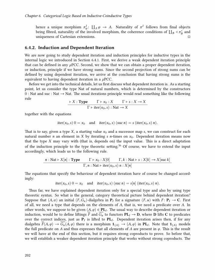
Chapter 6. Categorical Logic Based on Inductive-Coinductive Types
hence a unique morphism π Iϕ :
⨿A ϕ → A. Naturality of π I follows from final objects
being fibred, naturality of the involved morphism, the coherence conditions of⨿
B ⊣ π ∗B anduniqueness of Cartesian extensions.
6.4.2. Induction and Dependent IterationWe are now going to study dependent iteration and induction principles for inductive types in theinternal logic we introduced in Section 6.4.1. First, we derive a weak dependent iteration principlethat can be defined in any µPCC. Second, we show that we can obtain a proper dependent iteration,or induction, principle if we have strong sums. Since the second projection of strong sums can bedefined by using dependent iteration, we arrive at the conclusion that having strong sums is theequivalent to having dependent iteration in a µPCC.
Before we get into the technical details, let us first discuss what dependent iteration is. As a startingpoint, let us consider the type Nat of natural numbers, which is determined by the constructors0 : Nat and suc : Nat→ Nat. The usual iterations principle would read something like the followingrule
⊢ X : Type Γ ⊢ x0 : X Γ ⊢ s : X → X
Γ ⊢ iter(x0, s) : Nat→ X
together with the equations
iter(x0, s) 0 = x0 and iter(x0, s) (suc n) = s (iter(x0, s) n).
That is to say, given a type X , a starting value x0 and a successor map s , we can construct for eachnatural number n an element in X by iterating s n-times on x0. Dependent iteration means nowthat the type X may vary with (that is, depends on) the input value. This is a direct adaptationof the induction principle to the type theoretic setting.56 Of course, we have to extend the inputaccordingly, which leads us to the following rule.
n : Nat ⊢ X [n] : Type Γ ⊢ x0 : X [0] Γ,k : Nat ⊢ s : X [k]→ X [suc k]Γ,n : Nat ⊢ iter(x0, s) n : X [n]
The equations that specify the behaviour of dependent iteration have of course be changed accord-ingly:
iter(x0, s) 0 = x0 and iter(x0, s) (suc n) = s[n] (iter(x0, s) n).
Thus far, we have explained dependent iteration only for a special type and also by using typetheoretic syntax. So what is the general, category theoretical picture behind dependent iteration?Suppose that (A,α) an initial (F ,Gu)-dialgebra in PI for a signature (F ,u) with F : PI → C. Firstof all, we need a type that depends on the elements of A, that is, we need a predicate over A. Inother words, we suppose to be given (A,ϕ) ∈ PLI . The usual way to describe dependent iteration orinduction, would be to define liftings F and Gu to functors PLI → D, where D lifts C to predicatesover the correct indices, just as PI is lifted to PLI . Dependent iteration arises then, if for anydialgebra F (A,ϕ) → Gu(A,ϕ) there is a morphism 1A → (A,ϕ) in PLI . Note that 1A modelsthe full predicate on A and thus expresses that all elements of A are present in ϕ. This is the resultwe will have at the end of this section, but it requires strong coproducts to prove. So before that,we will establish a weaker dependent iteration principle that works without strong coproducts. The
202

6.4. Internal Reasoning Principles
idea is that we can track dependencies using sums, that is, given (A,ϕ) ∈ PLI , we can pack thispredicate to (A,ϕ)I = ⨿
A ϕ ∈ PI , see Lemma 6.4.1. This trick allows us to avoid having to moveto dialgebras on predicates and instead formulate dependent iteration simply on data types, as thefollowing proposition shows.
Proposition 6.4.2. Let (F ,u) be a signature with F : PI → C, (A,α) an initial (F ,Gu)-dialgebra, andd : F (A,ϕ)I → Gu (A,ϕ)I , such that π I
ϕ : (A,ϕ)I → A is a homomorphism. Then there is a uniquehomomorphism h : (A,α)→ ((A,ϕ)I ,d) with π I
ϕ h = idA as in the following diagrams.
F (A) F (A,ϕ)I F (A)
Gu(A) Gu (A,ϕ)I Gu(A)
α
Fh
d
Fπ Iϕ
α
Guh Guπ Iϕ
A (A,ϕ)I
A
!h
π Iϕ
Proof. The homomorphism h is the inductive extension of d and, since π Iϕ h is an endomorphism
on α , it must be the identity by uniqueness of inductive extensions.
Note that the condition π Iϕ being a homomorphism states that d only changes the element of ϕ,
but preserves the elements of A. The morphism h maps the elements of A to their correspondingelements of ϕ, and the assertion π I
ϕ h = id tells us that h keeps the index from A intact. Letus demonstrate the dependent iteration principle by deriving the classical induction principle forvectors.
Example 6.4.3. Recall that we defined vectors as the initial (F ,Gu)-dialgebra with F = ⟨1,KA × Id⟩and Gu = ⟨z∗, s∗⟩, giving rise to the constructor α = (nil, cons). In this case, the condition that πNϕis a homomorphism for a map d = (d1,d2) becomes
d1 : 1→ z∗(⨿
VecA(ϕ)
)z∗
(πNϕ
) d1 = nil
d2 : A ×⨿
VecA(ϕ)→ s∗
(⨿VecA
(ϕ))
s∗(πNϕ
) d2 = cons
(idA × πNϕ
),
which are, modulo the use of coproducts, the usual condition for induction base and step.Let us derive from Proposition 6.4.2 an induction principle for predicates on vectors that have
only trivial proofs for membership. More precisely, let Ψ ⊑ VecA be a predicate in SetN, where⊑ denotes the index-wise set inclusion. We can derive from Ψ a predicate ϕ ∈ SetVec A in theinternal logic of Fam(Set) by defining
ϕ(n,v) =
1, v ∈ Ψn
∅, otherwise.
Our goal is now to derive the following induction principle for Ψ by using Proposition 6.4.2 on ϕ.
nil ∗ ∈ Ψ0 ∀n ∈ N. ∀a ∈ A. ∀v ∈ (Vec A)n .v ∈ Ψn =⇒ cons a v ∈ Ψn+1
VecA ⊑ Ψ(6.12)
The premises of the rule (6.12) allow us to define maps d1 and d2 as above by putting
d1(⋆) B (nil⋆,⋆) d2(a, (v,⋆)) B (cons a v,⋆).
203
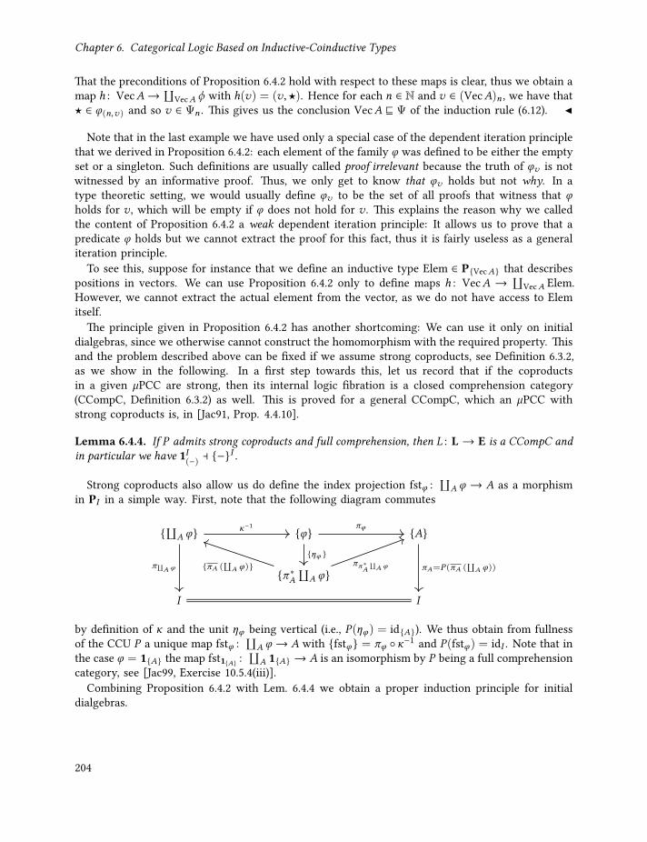
Chapter 6. Categorical Logic Based on Inductive-Coinductive Types
That the preconditions of Proposition 6.4.2 hold with respect to these maps is clear, thus we obtain amap h : VecA→⨿
VecA φ with h(v) = (v,⋆). Hence for each n ∈ N and v ∈ (VecA)n , we have that⋆ ∈ ϕ(n,v) and so v ∈ Ψn . This gives us the conclusion VecA ⊑ Ψ of the induction rule (6.12).
Note that in the last example we have used only a special case of the dependent iteration principlethat we derived in Proposition 6.4.2: each element of the family ϕ was defined to be either the emptyset or a singleton. Such definitions are usually called proof irrelevant because the truth of ϕv is notwitnessed by an informative proof. Thus, we only get to know that ϕv holds but not why. In atype theoretic setting, we would usually define ϕv to be the set of all proofs that witness that ϕholds for v , which will be empty if ϕ does not hold for v . This explains the reason why we calledthe content of Proposition 6.4.2 a weak dependent iteration principle: It allows us to prove that apredicate ϕ holds but we cannot extract the proof for this fact, thus it is fairly useless as a generaliteration principle.
To see this, suppose for instance that we define an inductive type Elem ∈ PVecA that describespositions in vectors. We can use Proposition 6.4.2 only to define maps h : VecA → ⨿
VecA Elem.However, we cannot extract the actual element from the vector, as we do not have access to Elemitself.
The principle given in Proposition 6.4.2 has another shortcoming: We can use it only on initialdialgebras, since we otherwise cannot construct the homomorphism with the required property. Thisand the problem described above can be fixed if we assume strong coproducts, see Definition 6.3.2,as we show in the following. In a first step towards this, let us record that if the coproductsin a given µPCC are strong, then its internal logic fibration is a closed comprehension category(CCompC, Definition 6.3.2) as well. This is proved for a general CCompC, which an µPCC withstrong coproducts is, in [Jac91, Prop. 4.4.10].
Lemma 6.4.4. If P admits strong coproducts and full comprehension, then L : L → E is a CCompC andin particular we have 1I
(−) ⊣ −I .
Strong coproducts also allow us do define the index projection fstϕ :⨿
A ϕ → A as a morphismin PI in a simple way. First, note that the following diagram commutes
⨿A ϕ ϕ A
π ∗A⨿
A ϕ
I I
κ−1
π⨿A ϕ
πϕ
ηϕ πA=P(πA (
⨿A ϕ))πA (
⨿A ϕ) ππ ∗A
⨿A ϕ
by definition of κ and the unit ηϕ being vertical (i.e., P(ηϕ ) = idA). We thus obtain from fullnessof the CCU P a unique map fstϕ :
⨿A ϕ → A with fstϕ = πϕ κ−1 and P(fstϕ ) = idI . Note that in
the case ϕ = 1A the map fst1A :⨿
A 1A → A is an isomorphism by P being a full comprehensioncategory, see [Jac99, Exercise 10.5.4(iii)].
Combining Proposition 6.4.2 with Lem. 6.4.4 we obtain a proper induction principle for initialdialgebras.
204
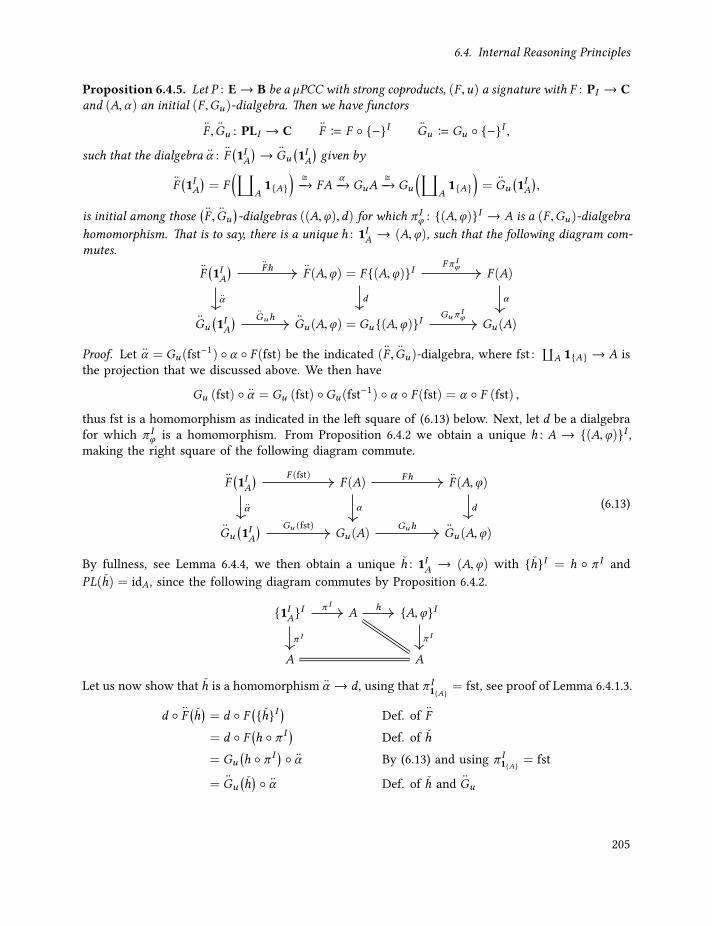
6.4. Internal Reasoning Principles
Proposition 6.4.5. Let P : E→ B be a µPCC with strong coproducts, (F ,u) a signature with F : PI → Cand (A,α) an initial (F ,Gu)-dialgebra. Then we have functors
F , Gu : PLI → C F B F −I Gu B Gu −I ,
such that the dialgebra α : F(1IA
)→ Gu
(1IA
)given by
F(1IA
)= F
(⨿A1A
)−→ FA
α−→ GuA−→ Gu
(⨿A1A
)= Gu
(1IA
),
is initial among those(F , Gu
)-dialgebras ((A,ϕ),d) for which π I
ϕ : (A,ϕ)I → A is a (F ,Gu)-dialgebrahomomorphism. That is to say, there is a unique h : 1IA → (A,ϕ), such that the following diagram com-mutes.
F(1IA
)F (A,ϕ) = F (A,ϕ)I F (A)
Gu(1IA
)Gu(A,ϕ) = Gu (A,ϕ)I Gu(A)
α
F h
d
Fπ Iϕ
α
Guh Guπ Iϕ
Proof. Let α = Gu(fst−1) α F (fst) be the indicated (F , Gu)-dialgebra, where fst :⨿
A 1A → A isthe projection that we discussed above. We then have
Gu (fst) α = Gu (fst) Gu(fst−1) α F (fst) = α F (fst) ,
thus fst is a homomorphism as indicated in the left square of (6.13) below. Next, let d be a dialgebrafor which π I
ϕ is a homomorphism. From Proposition 6.4.2 we obtain a unique h : A → (A,ϕ)I ,making the right square of the following diagram commute.
F(1IA
)F (A) F (A,ϕ)
Gu(1IA
)Gu(A) Gu(A,ϕ)
α
F (fst)
α
Fh
d
Gu (fst) Guh
(6.13)
By fullness, see Lemma 6.4.4, we then obtain a unique h : 1IA → (A,ϕ) with hI = h π I andPL(h) = idA, since the following diagram commutes by Proposition 6.4.2.
1IAI A A,ϕI
A A
π I
π I h
π I
Let us now show that h is a homomorphism α → d , using that π I1A = fst, see proof of Lemma 6.4.1.3.
d F(h)= d F
(hI
)Def. of F
= d F(h π I ) Def. of h
= Gu(h π I ) α By (6.13) and using π I
1A = fst
= Gu(h) α Def. of h and Gu
205

Chapter 6. Categorical Logic Based on Inductive-Coinductive Types
Uniqueness of h is immediate by uniqueness of h and by the comprehension being faithful. Henceα is initial indeed.
Now that we have obtained a dependent iteration (or induction) principle from uniqueness ofinductive extensions and strong coproducts, one may ask if we can also go the other way round.That is to say, can we state a dependent iteration principle without appealing to strong coproductsand then derive the existence of an inverse for the coproduct injection from there? We will answerthe first question affirmatively here, but leave the second to the syntactic development in Chapter 7.The reason for deferring the second part is that the answer to the first question is unfortunately verytechnical and should merely be seen as a possibility result, not a practically usable result. One canformulate the result differently as to obtain a better usable result but that requires us to manuallydefine a lifting for the strictly positive type functors in Definition 6.2.9. This is certainly possiblebut then we would do the same again in the syntactic development, thereby repeating a lot of work.Cutting a long story short, we will now adapt the development of an induction principle by Fumexet al. [FGJ11] to our setting of dependent iteration for inductive types without appealing to strongcoproducts.
In [FGJ11], Fumex et al. define a generic lifting for functors to predicates to be able to formulatean induction principle. A remarkable fact of this lifting is that it does not use any further propertiesof the functor that it lifts, only the fact that comprehension is right adjoint to the final object functor.However, in our case we would thus need for each I ∈ B that −I is right adjoint to 1I
(−), whichin turn needs that the coproducts in the fibration P are strong, see Lemma 6.4.4. Since we want toavoid requiring that, we restate the result in [GJF12, Thm. 4.14] under weaker conditions, namelywithout using the full adjunction 1I
(−) ⊣ −I .
Lemma 6.4.6. If P : E→ B is a µPCC, then there are functors LI : PLI → P→I and U I : P→I → PLI , ofwhich LI is given by LI (A,ϕ) = π I
ϕ :⨿
A ϕ → A. Moreover, given a functor F : PI → PJ , then there is afunctor F→ : P→I → P→J defined by F→(f : A→ B) = F f : FA→ FB. Out of these,U I and F→ preservefinal objects and, if P has full comprehension, then also LI preserves final objects.
Proof. Functoriality of LI follows readily from π I being a natural transformation. U I is given, asin [GJF12], by
U I (f : A→ B) =⨿
f(1IA) =
⨿f(A, 1A) =
(B,
⨿f
1A),
where the coproduct⨿
f is taken in LI (Lemma 6.4.1) The definition of U I on morphisms is slightlymore complicated, see loc. cit., we note however that it only uses properties of cartesian liftings.Finally, F→ is the canonical lifting of a functor to arrow categories.
The proof that U I preserves final objects is given by Ghani et al. [GJF12, Thm. 4.14], and thepreservation of final objects by F→ is a routine proof. That LI preserves final objects means thatit maps 1IA =
(A, 1A
)to an isomorphism. This is indeed the case here, as, by fullness, the map
π Iϕ :
⨿A 1A → A is an isomorphism, see [Jac99, Ex. 10.5.4]. The rest of the proof in [GJF12] can
be preserved.
As in [FGJ11], we can combine these functors into a lifting of functors F : PI → PJ to predicates.
206

6.4. Internal Reasoning Principles
Definition 6.4.7. The canonical predicate lifting of a functor F : PI → PJ is given by
F B PLILI−−→ P→I
F→−−→ P→JU J
−−→ PLJ .
This extends to a canonical predicate lifting of a signature (F ,u) with F : PI →∏
k=1, ...,n PJk to (F ,u)
with F : PLI →∏
k=1, ...,n PLJk by putting
Fk B PLILI−−→ P→I
F→k−−→ P→JkU Jk−−−→ PLJk .
Note that the functor Gu associated to this signature is then given by
Gu = ⟨u#1, . . . ,u
#n⟩ : PI →
∏n
k=1PLJk ,
where the reindexing is now taken in the internal logic L.
The liftings F and Gu preserve fibred final objects by Lem. 6.4.6 and by reindexing preservingfibred structure, respectively. This gives us the following important property of the canonical liftings,which enables us to express a dependent iteration principle.
Lemma 6.4.8. The canonical predicate lifting of a signature (F ,u) is truth-preserving, in the sense that
F 1I(−) (
n∏k=1
1Jk(−)
) F and Gu 1I(−)
(n∏
k=1
1Jk(−)
)Gu .
Let us briefly discuss what shape the dialgebras for these lifted functors take in Fam(Set).
Example 6.4.9. Recall that an object in PLI is a pair (A,ϕ) with ϕ ∈ PA . Let us first spell outhow F and Gu act component-wise on such objects.
Fk (A,ϕ) = U Jk F→k LI (A,ϕ)
= U Jk F→k
(fstϕ :
⨿Aϕ → A
)= U Jk
(Fk (fstϕ ) : Fk
(⨿Aϕ)→ FkA
)=
(FkA,
⨿Fk (fstϕ )
1Fk (⨿A ϕ)
)and
Gu,k (A,ϕ) = u#k (A,ϕ)
=(u∗k A, uk A
∗ ϕ)
= (Gu,kA, uk A∗ ϕ)
A morphism r : F (A,ϕ)→ Gu(A,ϕ) in∏n
k=1 PLJk is now an n-tuple of pairs ((d1,b1), . . . , (dn ,bn)),such that (d1, . . . ,dn) : FA→ GuA is an (F ,Gu)-dialgebra, and each bk is a morphism
bk :⨿Fk (fstϕ )
1Fk (⨿A ϕ) → uk A∗ ϕ
207

Chapter 6. Categorical Logic Based on Inductive-Coinductive Types
with dk = P(bk ). Recall that comprehension in Fam(Set) was given by taking coproducts. Thus,for A ∈ SetI we have FkA =
⨿j ∈Jk (FkA)j and the elements of FkA are of the form (j,x) with
j ∈ Jk and x ∈ (FkA)j . Given ϕ ∈ SetA , we have for (j,x) ∈ FkA(⨿Fk (fstϕ )
1Fk (⨿A ϕ)
)(j,x)
=⨿
(j′,y) ∈ Fk (⨿
A ϕ)j′=j and Fk (fstϕ )j (y) = x
1 ⨿
y ∈ Fk (⨿
A ϕ)jFk (fstϕ )j (y) = x
1,
from where we obtain that the components of bk have the following type.
(bk )(j,x) :⨿
y ∈ Fk (⨿
A ϕ)jFk (fstϕ )j (y) = x
1 −→ ϕ(uk (j),dk, j (x)).
Most importantly, note the use of dk in the codomain of bk , which comes from the fact thatdk = P(bk ). The intuition is that each bk proves, from the induction hypothesis that ϕ holds atthe argument of the constructor dk , that ϕ holds at dk, j(x).
Let us spell this example further out in the case when A is the family of vectors of a set B. Thus,we assume, see Example 6.2.4, that F : SetN → Set1 × SetN with F1 = K1 and F2 = !∗N(B) × Id, andG(u1,u2) = ⟨z∗, s∗⟩. Recall that we called the constructors for vectors nil and cons, so that we nowput d1 = nil and d2 = cons. Given a predicate ϕ ∈ SetList B that we want to prove by induction, weneed to provide maps b1 and b2 of the following type. For b1, note that F1(List B) =
⨿x ∈1 1 1,
so that there only needs to be a single map b1 of type
b1 :⨿y ∈ 1
id(y) =⋆
1 −→ ϕ(0,nil(⋆)).
For b2, we note that elements of F2(List B) are given by pairs (n, (b,x)) where n ∈ N and(b,x) ∈ B × (List B n). Thus, we have
(b2)(n,(b,x)) :⨿
(b,u) ∈ F2(⨿
ListB ϕ)nfstϕ (u) = x
1 −→ ϕ(n+1,consn(b,x)).
We can now read the types of b1 and b2 as follows. Firstly, the map b1 picks out a proof that ϕholds for the empty vector nil(⋆). Second, for a fixed n ∈ N, b ∈ B and x ∈ List B n, we can refinethe domain of (b2)(n,(b,x)) further. Note that u ∈ (⨿ListB ϕ)n is a pair (x ′,p), where x ′ ∈ List B n andp ∈ ϕ(n,x ′). The constraint that fstϕ (u) = x ensures then that x ′ = x . In other words, the domain ofb2 consists essentially of all proofs of ϕ(n,x). These observations allow us to rewrite the type of b2to the following.
(b2)(n,(b,x)) : ϕ(n,x) → ϕ(n+1,consn(b,x))
In this form, we recognise immediately the assumptions of the expected induction scheme for vectors,if we use a proof-irrelevant ϕ as in Example 6.4.3.
ϕ(0,nil(⋆)) ∀n ∈ N. ∀b ∈ B. ∀x ∈ List B n.ϕ(n,x) → ϕ(n+1,consn(b,x))
∀n ∈ N. ∀x ∈ List B n.ϕ(n,x)
208

6.4. Internal Reasoning Principles
We will discuss the case for a predicate ϕ that is not defined to be proof-irrelevant in Example 6.4.11.
What remains is to define dependent iteration using the canonical predicate lifting.
Definition 6.4.10. There is a functor
DiAlg(1) : DiAlg(F ,Gu)→ DiAlg(F ,Gu)
given on objects d : FX → GuX by
DiAlg(1)(d) = F(1IX
)
n∏k=1
1JkF (X )
∏nk=1
1Jkd−−−−−−−−→n∏
k=1
1JkGu (X ) Gu
(1IX
),
using that the canonical lifting is truth-preserving, see Lemma 6.4.8. We say that a µPCC P : E→ Badmits dependent iteration, if DiAlg(1) preserves initial dialgebras, cf. [HJ97].
Let us explicate this form of dependent iteration for vectors, thereby continuing Example 6.4.9.
Example 6.4.11. Recall that for a predicate ϕ ∈ SetList B we were able to reduce the conditionson a dialgebra r : F (List B,ϕ)→ Gu(List B,ϕ) with r = ((nil,b1), (cons,b2)) to
b1 : 1→ ϕ(0,nil(⋆)) and (b2)(n,(b,x)) : ϕ(n,x) → ϕ(n+1,consn(b,x)).
If P happens to admit dependent iteration, then there is a unique homomorphism h : 1IList B →(List B,ϕ). Since 1IList B = (List B, 1List B ), we have that h = (f ,д), where f and д are maps withf : List B → List B and д : 1List B → ϕ. Moreover, for f the following diagram commutes.
F (List B) F (List B)
Gu(List B) Gu(List B)
F f
(nil,cons) (nil,cons)Gu f
From uniqueness of inductive extensions, we thus immediately conclude that f is the identity map.For the map д, the following diagram commutes for any choice of n ∈ N, b ∈ B and x ∈ List B n.
(1, (1List B )(n,x)) (1,ϕ(n,x))
((1List B )(0,nil(⋆)), (1List B )(n+1,consn(b,x))) (ϕ(0,nil(⋆)),ϕ(n+1,consn(b,x)))
(id1, id1)
(id,д(n,x))
(b1,(b2)(n,(b,x)))(д(0,nil(⋆)),д(n+1,consn (b,x)))
This diagram expresses the expected computational behaviour of dependent recursion.To sum the above discussion up, let us state the following dependent iteration rule for vectors in
Fam(Set), in which we use dependent products to express the type constraints of b1 and b2 moreconveniently.
b1 : 1→ ϕ(0,nil(⋆)) b2 : Πn ∈ N.Πb ∈ B.Πx ∈ List B n.ϕ(n,x) → ϕ(n+1,consn(b,x))
д : Πn ∈ N.Πx ∈ List B n. 1→ ϕ(n,x)
209

Chapter 6. Categorical Logic Based on Inductive-Coinductive Types
The second diagram above expresses then indeed the expected computational behaviour:
д(0, nil(⋆))(⋆) = b1(⋆)
д(n + 1, consn(b,x))(⋆) = (b2)(n,(b,x))(д(n,x)(⋆))
With this, we end our exploration of dependent iteration and induction in the context of categoricaldependent inductive types. It is time to move on to its dual: coinduction.
6.4.3. CoinductionIn the last section we have discussed dependent iteration principles for inductive types. Underthe BHK-interpretation, these dependent iteration principles give us then also induction principles,with which we can prove predicates to hold on all elements of an inductive type. This raises ofcourse the question what the corresponding principle for coinductive types is. Since elements ofcoinductive types allow the description and comparison of behaviour, Hermida and Jacobs [HJ97]observed that the canonical proof principle associated with coalgebras is concerned with provingequality. More specifically, the principle of coinduction grants us the possibility to prove an identitybetween elements of a coinductive type by establishing a bisimulation relation. The goal of thissection is to provide a simple coinduction principle for coinductive types in a recursive-type closedcategory (µPCC).
To state what a bisimulation relation for a coinductive type is, we first need to define relationsinternal to a µPCC, where by relation we mean here binary relations on one carrier. Intuitively, suchrelations are given as predicates on the binary product of that carrier with itself. Since the carriermight be a dependent type, we need to take those dependencies into account. These considerationsleads us to define the category of relations in the internal logic of P as the following pullback of LIalong ∆, where ∆ is the diagonal given by ∆(A) = A ×I A and the binary product is taken in PI ,see Theorem 6.2.11.
Rel(PI ) PLI
PI PI
LI
∆
We will usually leave out the subscript of the binary product, if the index I is understood from thecontext. Intuitively, Rel(PI ) consists of objects (A,R) with A ∈ PI and R ∈ PA×A . The morphismsin Rel(PI ) are pairs (f ,д) : (A,R) → (A′,R′) with f : A → A′, д : R → R′ and Pд = f ×I f , cf.Section 6.4.1.
To define relation liftings, Fumex et al. [FGJ11] use a so-called quotient functor Q : Rel(PI )→ PI .Such a functor intuitively takes (A,R) to the quotient of A by the equivalence closure of R. We willnot need a full quotient here to formulate a coinduction principle, rather it suffices to take insteadthe collection of pairs in A together with a proof that these are related. The reason for this is thatthe coinduction principle is only valid on final dialgebras, hence there is no need to take a quotientto compare states of other dialgebras under behavioural equivalence. So let us define a functorQ : Rel(PI )→ PI by
Q(A,R) B (A ×A,R)I =⨿
A×AR. (6.14)
Similar to the weak dependent iteration principle, we will now use Q to establish a coinductionprinciple by appealing to the fact that coinductive types admit unique coinductive extensions. To
210
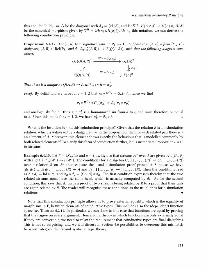
6.4. Internal Reasoning Principles
this end, let δ : IdPI ⇒ ∆ be the diagonal with δA = ⟨id, id⟩, and let ∇H : H(A×A)→ H(A)×I H(A)be the canonical morphism given by ∇H = ⟨H(π1),H(π2)⟩. Using this notation, we can derive thefollowing coinduction principle.
Proposition 6.4.12. Let (F ,u) be a signature with F : PI → C. Suppose that (A, ξ ) a final (Gu , F )-dialgebra, (A,R) ∈ Rel(PI ) and d : Gu(Q(A,R)) → F (Q(A,R)), such that the following diagram com-mutes.
Gu(Q(A,R)) Gu(A)2
F (Q(A,R)) F (A)2
d
∇Gu Gu (π IR )
ξ×I ξ∇F F (π IR )
Then there is a unique h : Q(A,R)→ A with δA h = π IR .
Proof. By definition, we have for i = 1, 2 that πi ∇Gu = Gu(πi ), hence we find
πi ∇Gu Gu(πIR) = Gu(πi π I
R),
and analogously for F . Thus πi π IR is a homomorphism from d to ξ and must therefore be equal
to h. Since this holds for i = 1, 2, we have π IR = δA h.
What is the intuition behind this coinduction principle? Given that the relation R is a bisimulationrelation, which is witnessed by a dialgebra d as in the proposition, then for each related pair there is aan element of A. Moreover, this element shows exactly the behaviour that is modelled commonly byboth related elements.57 To clarify this form of coinduction further, let us instantiate Proposition 6.4.12to streams.
Example 6.4.13. Let F = ⟨KA, Id⟩ and u = (id1, id1), so that streams Aω over A are given by ν(Gu , F )with (hd, tl) : Gu(A
ω)→ F (Aω). The conditions for a dialgebra Gu(⨿
Aω×Aω (R))→ (A,⨿
Aω×Aω (R))over a relation R on Aω then capture the usual bisimulation proof principle: Suppose we have(d1,d2) with d1 :
⨿Aω×Aω (R) → A and d2 :
⨿Aω×Aω (R) →
⨿Aω×Aω (R). Then the conditions read
as δ d1 = hd πR and πR d2 = (tl × tl) πR . The first condition expresses thereby that the tworelated streams must have the same head, which is actually computed by d1. As for the secondcondition, this says that d2 maps a proof of two streams being related by R to a proof that their tailsare again related by R. The reader will recognise these conditions as the usual ones for bisimulationrelations.
Note that this coinduction principle allows us to prove external equality, which is the equality ofmorphisms in E, between elements of coinductive types. This includes also the (dependent) functionspace, see Theorem 6.2.11. In particular, we can show in this case that functions are equal by provingthat they agree on every argument. Hence, for a theory in which functions are only externally equalif they are convertible, we need to relax the requirement that coinductive types are final dialgebras.This is not so surprising, and we will discuss in Section 6.6 possibilities to overcome this mismatchbetween category theory and syntactic type theory.
211

Chapter 6. Categorical Logic Based on Inductive-Coinductive Types
6.5. A Beck-Chevalley Condition for Recursive TypesAs already mentioned in the introduction, if we want to recover the expected property that substitu-tions distribute over sum types, then we need to require that the so-called Beck-Chevalley conditionholds for coproducts. More specifically, given a term t and variables x and y, such that x is distinctfrom all the variables in t and from y, one defines substitution on sum types by
(Σx : A[y]. B[x ,y])[t/y] = Σx : A[t ]. B[x , t ].
Notice that there is something subtle is going on here. First, the sum on the right is a different onebecause the type of the variable x has changed. Second, we assumed that the variable x is distinctfrom all other variables around, which allows to avoid having to rename x . More generally, we couldintroduce a fresh name, rename the bound occurrences of x in B and then define the substitutionon sums by
(Σx : A[y]. B[x ,y])[t/y] = Σx ′ : A[t ]. B[x ′, t ]. (6.15)
We will now use the classifying fibration for a dependent type theory, which we introducedin Section 6.1, to explain how the Beck-Chevalley condition captures this definition of substitutioncategory theoretically. Recall that we defined the coproduct as a left-adjoint functor to the projectionsπA : A → PA. In the context of the classifying fibration for a dependently typed calculus, wedefined comprehension as context extension and the projections are the weakening substitutions.More precisely, for a context Γ = x1 : A1, . . . ,xn : An , a type A with Γ ⊢ A : Type and a freshvariable x comprehension is given by Γ ⊢ A : Type = Γ,x : A. The corresponding projectionπA : Γ,x : A → Γ is given by πA = (x1, . . . ,xn). This allows us to express the equation (6.15) incategory theoretical terms by using the coproduct as follows. Suppose that y : C ⊢ A : Type andΓ ⊢ t : C , then equation (6.15) reads as(⨿
πAB[x ,y]
)[t/y] =
⨿πA[t ]
B[x ′, t ].
Using that reindexing amounts to the application of substitutions, we can further rewrite this to:
t∗(⨿
πA[y]B[x ,y]
)=
⨿πA[t ]
(t ,x ′)∗(B[x ,y]).
Note that the involved substitutions and projections can be organised in the following pullbackdiagram.
Γ,x ′ : A[t ] Γ
y : C,x : A y : C
πA[t ]
(t,x ′) t
πA
The fact that this is a pullback diagram captures the essence of the variable renaming and therebyalso the interaction between the involved coproduct and reindexing functors.
Let us now generalise this interaction between reindexing and coproducts to arbitrary coproducts.The above considerations lead us then to assume that we are given a pullback square such as the
212
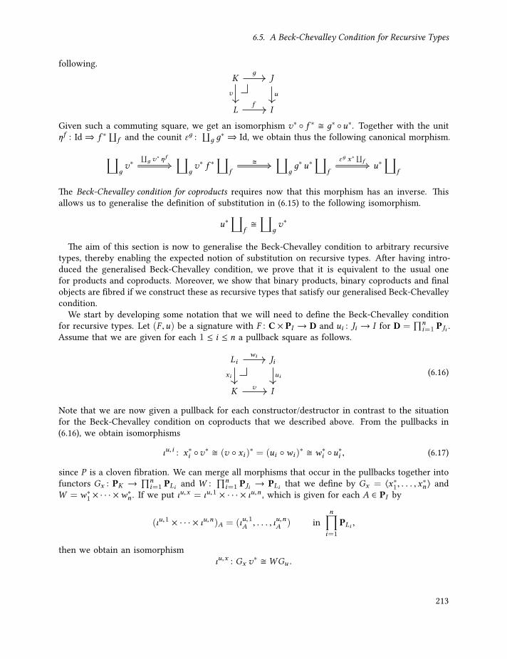
6.5. A Beck-Chevalley Condition for Recursive Types
following.K J
L I
д
v uf
Given such a commuting square, we get an isomorphism v∗ f ∗ д∗ u∗. Together with the unitηf : Id⇒ f ∗
⨿f and the counit εд :
⨿д д∗ ⇒ Id, we obtain thus the following canonical morphism.⨿
дv∗
⨿дv∗ f ∗
⨿f
⨿дд∗ u∗
⨿f
u∗⨿
f
⨿д v∗ ηf εд x ∗
⨿f
The Beck-Chevalley condition for coproducts requires now that this morphism has an inverse. Thisallows us to generalise the definition of substitution in (6.15) to the following isomorphism.
u∗⨿
f
⨿дv∗
The aim of this section is now to generalise the Beck-Chevalley condition to arbitrary recursivetypes, thereby enabling the expected notion of substitution on recursive types. After having intro-duced the generalised Beck-Chevalley condition, we prove that it is equivalent to the usual onefor products and coproducts. Moreover, we show that binary products, binary coproducts and finalobjects are fibred if we construct these as recursive types that satisfy our generalised Beck-Chevalleycondition.
We start by developing some notation that we will need to define the Beck-Chevalley conditionfor recursive types. Let (F ,u) be a signature with F : C × PI → D and ui : Ji → I for D =
∏ni=1 PJi .
Assume that we are given for each 1 ≤ i ≤ n a pullback square as follows.
Li Ji
K I
wi
xi ui
v
(6.16)
Note that we are now given a pullback for each constructor/destructor in contrast to the situationfor the Beck-Chevalley condition on coproducts that we described above. From the pullbacks in(6.16), we obtain isomorphisms
ιu,i : x∗i v∗ (v xi )∗ = (ui wi )∗ w∗i u∗i , (6.17)
since P is a cloven fibration. We can merge all morphisms that occur in the pullbacks together intofunctors Gx : PK →
∏ni=1 PLi and W :
∏ni=1 PJi → PLi that we define by Gx = ⟨x∗1, . . . ,x∗n⟩ and
W = w∗1 × · · · ×w∗n . If we put ιu,x = ιu,1 × · · · × ιu,n , which is given for each A ∈ PI by
(ιu,1 × · · · × ιu,n)A = (ιu,1A , . . . , ιu,nA ) in
n∏i=1
PLi ,
then we obtain an isomorphismιu,x : Gx v
∗ WGu .
213
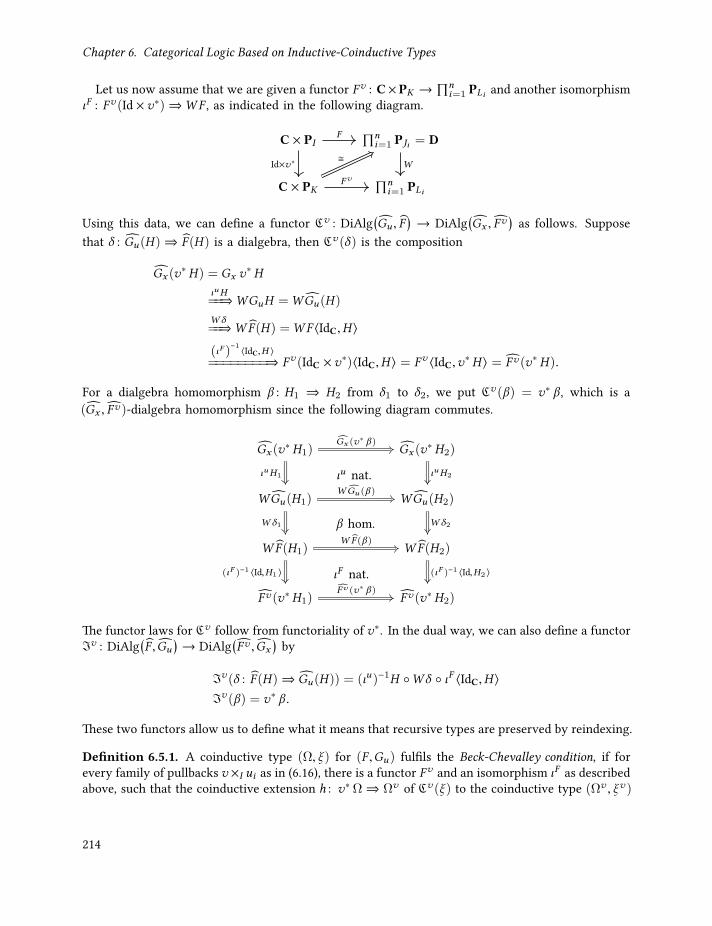
Chapter 6. Categorical Logic Based on Inductive-Coinductive Types
Let us now assume that we are given a functor Fv : C×PK →∏n
i=1 PLi and another isomorphismιF : Fv (Id ×v∗)⇒WF , as indicated in the following diagram.
C × PI∏n
i=1 PJi = D
C × PK∏n
i=1 PLi
F
Id×v∗ W
Fv
Using this data, we can define a functor Cv : DiAlg(Gu , F
)→ DiAlg
(Gx , Fv
)as follows. Suppose
that δ : Gu(H)⇒ F (H) is a dialgebra, then Cv (δ) is the composition
Gx (v∗H) = Gx v
∗H
ιuH==⇒WGuH =WGu(H)
W δ==⇒W F (H) =WF ⟨IdC,H ⟩(ιF )
−1 ⟨IdC,H ⟩========⇒ Fv (IdC ×v∗)⟨IdC,H ⟩ = Fv ⟨IdC,v∗H ⟩ = Fv (v∗H).
For a dialgebra homomorphism β : H1 ⇒ H2 from δ1 to δ2, we put Cv (β) = v∗ β , which is a(Gx , Fv )-dialgebra homomorphism since the following diagram commutes.
Gx (v∗H1) Gx (v
∗H2)
WGu(H1) WGu(H2)
W F (H1) W F (H2)
Fv (v∗H1) Fv (v∗H2)
Gx (v∗ β)
ιuH1 ιu nat. ιuH2
WGu (β)
W δ1 β hom. W δ2
W F (β)
(ιF )−1 ⟨Id,H1 ⟩ ιF nat. (ιF )−1 ⟨Id,H2 ⟩
Fv (v∗ β)
The functor laws for Cv follow from functoriality of v∗. In the dual way, we can also define a functorIv : DiAlg
(F , Gu
)→ DiAlg
(Fv , Gx
)by
Iv (δ : F (H)⇒ Gu(H)) = (ιu)−1H W δ ιF ⟨IdC,H ⟩Iv (β) = v∗ β .
These two functors allow us to define what it means that recursive types are preserved by reindexing.
Definition 6.5.1. A coinductive type (Ω, ξ ) for (F ,Gu) fulfils the Beck-Chevalley condition, if forevery family of pullbacks v ×I ui as in (6.16), there is a functor Fv and an isomorphism ιF as describedabove, such that the coinductive extension h : v∗Ω⇒ Ωv of Cv (ξ ) to the coinductive type (Ωv , ξv )
214

6.5. A Beck-Chevalley Condition for Recursive Types
for (Fv ,Gx ), as in the following diagram, is an isomorphism Cv (ξ ) ξv of dialgebras.
Gx (v∗ Ω) Gx (Ω
v )
Fv (v∗ Ω) Fv (Ωv )
Cv (ξ )
Gx (h)
ξv
Fv (h)
The Beck-Chevalley condition for inductive types is defined dually using Iv .
As the name suggests, this definition is supposed to capture the known Beck-Chevalley conditions.To prove this, we first need a small technical following.
Lemma 6.5.2. Let F1 : C1 → C2 be a functor and (F2,u) be a signature with F2 : C2 × PI → C3. Wedefine a functor F : C1 × PI → C3 by F = F2 (F1 × Id). With this definition, we have µ(F , Gu) =
µ(F2, Gu) F1 and α (F ,Gu ) = α (F2,Gu )F1. Dually, we also have that ν(Gu , F ) = ν(Gu , F2) F1 andξ (F ,Gu ) = ξ (F2,Gu )F1.
Proof. This follows simply from the definitions. Let V ∈ C1, then
µ(F , Gu)(V ) = µ(F (V ,−),Gu) = µ((F2 (F1 × Id))(V ,−),Gu)
= µ(F2(F1(V ),−),Gu) = µ(F2, Gu)(F1(V ))
= (µ(F2, Gu) F1)(V )
and the equality of the natural transformations follows immediately from their definition and thefunctor equality above.
We can now show the usual Beck-Chevalley condition and the one given in Definition 6.5.1 areequivalent for the adjunctions we obtained as recursive types in Theorem 6.2.11.
Theorem 6.5.3. The adjunctions constructed inTheorem 6.2.11 are fibred iff they fulfil the Beck-Chevalleycondition for recursive types.
Proof. We prove this for the constructed right adjoints, the proof for the left adjoints follows byduality. Recall that we defined for C =
∏ni=1 PJi , a right adjoint for all Gu = ⟨u∗1, . . . ,u∗n⟩ by
ν(Gu , π1) : D → PI with π1 : C × PI → C. Given pullbacks (xi ,wi ) = v ×I ui as in (6.16), we putD =
∏ni=1 PLi ,W : C→ D withW = w∗1 × · · · ×w∗1 and Gx = ⟨x∗1, . . . ,x∗n⟩. We find the right adjoint
of Gx to be ν(Gx , π′1) with π ′1 : D × PK → D. The Beck-Chevalley condition (B-C condition) for
adjoint functors requires that the canonical natural transformation γ : v∗ ν(Gu , π1)⇒ ν(Gx , π′1)W
is an isomorphism. We show that this coincides with our definition for recursive types.Let ξ be the final (Gu , π1)-dialgebra and ξv the final (Gx , Fv )-dialgebra. We note that for the
projection π ′′1 : C × PK → C, we have π ′1 (W × Id) = W π ′′1 . Thus, we can choose for the B-Ccondition Fv =W π ′′1 and get, by Lemma 6.5.2, ν(Gx , Fv ) = ν(Gx , π
′1) W . By finality, this means
that γ is in fact the unique morphism from Cv (ξ ) to ξv . The B-C condition for recursive typesrequires this to be an isomorphism, just as the B-C condition for adjoints does. This means thatthe constructed adjunctions are fibred iff they satisfy the B-C condition for recursive types with thechoice Fv =W π ′′1 .
215

Chapter 6. Categorical Logic Based on Inductive-Coinductive Types
In the same way, we can relate fibred final objects and our Beck-Chevalley condition.
Theorem 6.5.4. Terminal objects 1I , constructed as ν(id∗I , IdPI ), are fibred iff they satisfy the Beck-Chevalley condition for recursive types.
Proof. We note that the pullback (6.16) degenerates, in this case, to only give a morphism v : K → I .Then we pick Idv = v∗ and the rest follows as in Theorem 6.5.3.
6.6. Discussion
In the previous Chapter 5 we established several approaches to reasoning about mixed inductive-coinductive programs. Among these approaches was a syntactic logic FOL together with a proofsystem. We realised at the end of Section 5.2 that we could implement the standard induction andcoinduction principles for non-mutual inductive or coinductive types but not for more general types,see Note 39, since the logic FOL is lacking the possibility to form fixed point formulas. However,adding fixed point formulas would force us to also add the corresponding proof rules to the logic,which are a mere adaption of the term formation rules for fixed point types in the calculus λµν . Tosave ourselves from duplicating rule sets and from repeating proofs of properties for the logic, wedecided to merge programming and reasoning into one language.
In the present chapter, we established a dependent type theory in the language of category theory,in which we can write the same programs as in the calculus λµν , as well as reason about theseprograms. The idea of this category theoretical language was to extend the ideas of Hagino [Hag87]from a simply typed calculus to a dependently typed one. Specifically, this meant that we viewedinductive and coinductive types as initial and final dialgebras in the fibres of a fibration. Thesefibres replaced thereby the simple categories that Hagino used and allowed us to manipulate thedependencies, as we have seen in the principle example of vectors in Section 6.2.1. Starting fromthis view on dependent types, we developed notions of signatures and strictly positive types thatform a general basis for dependent inductive-coinductive types. All these considerations led usto the definition of recursive type closed categories (µPCC) as a theory of inductive-coinductivedependent types. Besides the truly recursive types like vectors, (partial) streams, bisimilarity, andthe substream relation, we were also able to encode the standard connectives of Martin-Löf typetheory as (non-recursive) inductive and coinductive types. This will enable us in the next Chapter 7to construct a syntactic type theory that is purely based on recursive types, while still subsumingstandard Martin-Löf type theory.
After we introduced the basic category theoretical setup, we showed that the developed theoryis actually sensible by showing that the initial and final dialgebras can be constructed as initialalgebras and final coalgebras of polynomial functors. This opens up a wide class of models for thetheory. Moreover, we demonstrated that the unique mapping properties of inductive and coinductivetypes give rise to a simple dependent iteration (or induction) principle and a coinduction principle.Under the further assumption that coproducts are strong, that is, they admit projections for bothcomponents, we could also obtain a proper dependent iteration principle. Finally, we established aBeck-Chevalley condition for recursive types to allow the interpretation of a corresponding syntactictheory of inductive-coinductive dependent types in a µPCC.
216

6.6. Discussion
Related WorkLet us briefly discuss existing work that is related to the content of this chapter. Most of the relevantwork has been already discussed in the corresponding places, but a more streamlined overview seemsappropriate.
Categorical Dependent Recursive Types The basic setup, which we chose here to construedependent inductive-coinductive types category theoretically, is essentially a combination of existingideas. Specifically, we took Hagino’s dialgebra approach for simple types [Hag87] and merged itwith the fibrational view on dependent types [Jac99]. This fibrational view is, in my opinion, themost modular and transparent presentation of dependent types in terms of categories, since allrequirements made on a fibration have a clearly defined purpose. It is this modularity that makesfibrations very suitable for reusing existing notions in the context of inductive-coinductive dependenttypes. As mentioned at the end of Section 6.1, there is an abundant supply of category theoreticalmodels for dependent types. However, since these are specifically tailored towards dependent types,it is often the case that the straightforward approach of using dialgebras cannot be implemented there.Moreover, many of these models are related or even equivalent to fibrational models [Jac93]. Finally,we should mention that there are other category theoretical approaches to recursive dependent types,but none of them actually treats coinductive dependent types, see the introduction of Section 6.2.3.
Constructing Recursive Types as Polynomials Polynomial functors are the go-to class of func-tors that is used whenever reasonably general but also well-behaved class of functors are required.One of the main reasons for that is that they preserve certain limits and colimits [GK13], whichare important for constructing initial algebras [GH04; GK13; Koc11] and final coalgebras [Jac16;vdBdM07]. Another reason is that it is straightforward to associate a syntactic theory to initialalgebras [Fio12; HF11] and to final coalgebras [BRS09; Gol01] of polynomial functors, since theseare, respectively, finite and potentially infinite trees. This latter reason is also why polynomial func-tors [GK13; HF11] or container [Abb03; AAG05] are taken as foundation for data types. Fortunately,this interest led to many existing results that we were able to use in our reduction of theory ofdependent recursive types to polynomial functors in Section 6.3. The main sources that we usedhere were [GK13] and [AAG05].
Internal Reasoning Principles Both induction and coinduction principles have been studied ex-tensively in the context of category theory. The clearest expositions on these principles are [HJ97]and the extension [FGJ11] thereof to indexed sets. In Section 6.4, we instantiated some of the resultsfrom these two publications and proved other results under weaker conditions. This is discussed indetail in the corresponding places in Section 6.4.
A Beck-Chevalley Condition for Recursive Types The Beck-Chevalley condition is well- andwidely known for products and coproducts, but our analogue for recursive types has not been studiedanywhere. That being said, since products and coproducts arise as recursive types, one may askhow the classical Beck-Chevalley condition relates to ours in those cases. Indeed, in Theorem 6.5.3we showed that the classical condition is equivalent to ours for the presentation of products andcoproducts as recursive types.
217

Chapter 6. Categorical Logic Based on Inductive-Coinductive Types
Contributions
After summarising the content and context of the chapter, let us also clearly mark the contributionsmade in this chapter. First of all, the adaption of Hagino’s categorical data types to dependent typeshas not been explored before. Moreover, the resulting theory explains the types of Martin-Löf typetheory in terms of inductive-coinductive types, which was considered to some extend folklore but hasnever been formally explored somewhere. The construction of recursive types through polynomialsrequired one new result (Theorem 6.3.10), which is the main contribution of Section 6.3. Next, theinternal logic of a dependent type theory has, to the best of my knowledge, not been presentedand studied as we did in Section 6.4. In particular, the resulting (weak) induction and coinductionprinciples were not studied in the absence of strong coproducts and quotients. Since there was nocategory theoretical study of general dependent inductive-coinductive types, also the Beck-Chevalleycondition from Section 6.5 is a novel contribution.
Future Work
Much of the content in this chapter is fairly stable and explored. There are a few directions forfuture research though. As we will see in Chapter 7, the (unique) mapping principle of the recursivetypes from Section 6.2 correspond to simple iteration and coiteration rules on the syntactic side. Theproblem with this is that it usually much easier to write programs by giving a set of equations, similarto what we found in Section 3.2. This raises of course the question whether there is a way to giveequational specifications of morphisms on dependent recursive types. A possible approach mightbe to adapt, at least in the coinductive case, completely iterative algebras [Acz+03] to dependenttypes. However, the equational specifications there need to be extended with pattern matching forthe specification of functions on inductive types, and one needs to be careful with identity types, aspattern matching might lead to stronger than expected theories, cf. [CDP16; GMM06].
Since in Section 6.4 we found the internal reasoning principles were based on the fact that induct-ive and coinductive types come with unique mapping principles, we concluded that the categorytheoretical approach we took so far makes too strong requirements on types. The reason is thatuniqueness of inductive and coinductive extensions are problematic in syntactic theories becauseit usually breaks decidability of type checking. A possibility to overcome this problem is to makeuniqueness proof-relevant, in the sense that whenever we show the uniqueness of a homomorphism,then there is an explicit proof object in the category that witnesses this fact. This can be realised,for example, by using 2-categories or higher generalisations thereof. But since this takes us to farastray, we leave the problem of matching the category theoretical semantics better intensional typetheories for the future.
Notes41 Translation taken from “Substance and Function and Einsteins Theory of Relativity“ by E. Cassirer,
p.371, 1923.
42 For instance, having both projections for sum types in an impredicative calculus like the Calculusof Constructions, leads to inconsistencies, see [Coq89]. More precisely, the fact that there is a
218

6.6. Discussion
proposition isomorphic to the coproduct of a family of propositions is independent of having an im-predicative universe of propositions [Str89]. Similarly, a logic that combines computational classicallogic in form of control operators with strong sum types also becomes inconsistent, as has beenshown by Herbelin [Her05].
43 The alert reader might note that we only obtain (ListA (n + 1))[2] = ListA (2 + 1). To get to ListA 3we actually need to use the computation 2 + 1 ≡ 3 inside the type. Since this is not really relevantto the present introduction, we sweep this problem under the rug for now and come back to it inthe next chapter.
44 A more modern notation for dependent function types, which emphasises the close relation to thesimple function type, is (x : A) → B[x ] for Πx : A. B[x ]. However, since the dependent functionspace is given category theoretically as a product, we stick to the traditional notation here.
45 A historical overview can be found in [TvD88, Sec. 1.4].46 In modern expositions, System F is called λ2, see for example [NG14].47 The reverse direction of
∃x : A. ∀y : B.ϕ[x ,y] ⊢ ∀y : B. ∃x : A.ϕ[x ,y]
is the constructive version of the axiom of choice:
α : (∀x : A. ∃y : B.ϕ[x ,y]) ⊢ p : (∃f : A→ B. ∀x : A.ϕ[x , f x ]).
To give such a proof p, we need to assume though something more about the existential quantifier,namely that there are projections z : (∃x : A.ψ [x ]) ⊢ π1 z : A and z : (∃x : A.ψ [x ]) ⊢ π2 z : ψ [π1 z].How these can be obtained is discussed towards the end of Section 6.1 and in the next chapter. Ifwe have these projections, then the proof p is given by
p B⟨λx . π1 (α x), λx . π2 (α x)
⟩.
48 The propositions-as-types interpretation is often also referred to as Curry-Howard correspondence. Iwill, however, avoid this terminology here, since it is neither descriptive nor very accurate. Thereare many more people that would have to be mentioned in this name, first and foremost, Church ismissing from the list.
49 An exception is Frege’s definite description operator ι that allows one to name an object that uniquelysatisfies a proposition, see e.g. [TvD88, Par. 2.2.9] and [NG14, Sec. 12.7].
50 Of course, we can see isHoliday also as a predicate over the date type that we introduced above.However, we use the present definition for illustrative purposes later.
51 The adjunction⨿
I ⊣ !∗ consists in fact also of some equations that need to hold. As it turns out, one ofthese equations gives the computation rule for sum types: unpack ⟨u,v⟩ as ⟨i,x⟩ in t −→ t [u/i,v/x ].The other equation ensures that unpack y as ⟨i,x⟩ in t is the unique term with that computationalproperty, and as such is usually not part of a syntactic theory. Thus, the category theoretical
219

Chapter 6. Categorical Logic Based on Inductive-Coinductive Types
approach makes slightly to strong requirements here, see also the discussion in Section 4.2 for theanalogous situation in non-dependent calculi. This can be solved in the case of sum types by allowingη-conversions: unpack s as ⟨i,x⟩ in t [⟨i,x⟩/y] −→ t [s/y]. However, η-conversions are difficult tomanage and do not generalise well to recursive types.
52 There are two principal ways to conceive of vectors: Either we group the vectors of the same lengthinto a set, thereby forming a family of sets, or we see vectors as the set of all lists together withthe map that assigns to each list its length. In Example 6.2.1, we use the first view, but we will laterreturn to the second when we consider dependent types as objects in slice categories.
53 For an Agda-versed reader it might be interesting to note that the use of non-trivial substitutionin the domain of destructors is currently not available in Agda. It is questionable though whetheradding this capability is useful in an intensional theory like Agda. The reason is that if we are givenn : N∞ and t : PStr A n, then to apply hd to t we would have to establish that n = s∞ k for somek : N∞. However, since N∞ is a coinductive type, we will rarely find ourselves in the luxury positionthat we can prove an equality, rather we may only find that n is bisimilar to s∞ k for some k . Butan even better way would be to define PStr differently:
codata n : N∞ ⊢ PStr A n wherehd : PStr A n → (Π k : N∞. (n .out = κ2 k) → A)tl : PStr A n → (Π k : N∞. (n .out = κ2 k) → PStr A k)
Given an element s : PStrAn for some n : N∞, we can always apply, say, tl to s . This gives us thena term of type Πk . (n.out = κ2 k) → PStr A k . Thus, if we have a k of type N∞ and a proof p forn.out = κ2 k , then we obtain the tail of s by tl s k p : PStrAk . Such a definition works much betterin an intensional theory like Agda and, in contrast to a bisimilarity-based definition, still enablesthe use of automatic reductions.
54 Even though µP-complete categories offer more flexibility for the domain of the destructors of acoinductive type, see the note 53, the coinductive types in Agda provide some further power. Morespecifically, the destructors of a coinductive type in Agda can refer to previously declared destructors.This allows the declaration of a strong dependent sum, see [Jac99, Sec. 10.1 and Def. 10.5.2]. Wediscuss this in Section 6.4, and see also Note 47.
55 If X ∈ B/I and Y ∈ B/J , then a morphism f : X → Y in B can be defined in the internal language ofthe codomain fibration by statements of the form “fi p = e”, where p is a pattern and e an expressionthat are given by the following grammar.
e F x | f | e e | λp. e | (e, e)p F x | x : T | (p,p) | (p | c)c F e = e
T F I | Xe
The intention is that x is a variable, f a morphism in B, λp. e an element of a product, and (e, e)an element of a coproduct. A pattern is either a, possibly typed, variable, or it matches dependentpairs of a coproduct, or it introduces some constraints that arise from products or coproducts. Thoseconstraints may just be identities between expressions that can involve only the variables of the
220

6.6. Discussion
corresponding pattern. Finally, a type is either an object I of B or it selects a fibre Xe of X by meansof an expression. Typing constraints can then be given in the form e1 : Xe2 , which expresses thatX e1 = e2, using the fact that X is a morphism U → I for some object U in B. Expressions, patternsand constraints are all subject to the obvious typing constraints. For instance, given a morphismh : I → J in B and a morphism f : X → Y in B/I , we can define
⨿h f :
⨿h X →
⨿h Y by(⨿
hf)j(i,x : Xi | h i = j) = (i, f x).
We now need to show that (i, f x) : (⨿
h Y )j , i.e., h(Y (f x)) = j. Since f is a morphism in B/I ,we have that Y f = X . This gives us the required identity by using the constraint h i = j in thepattern of
⨿h f : h (Y (f x)) = h (X x) = h i = j.
56 Besides enabling induction, the dependent iteration allows also for interesting computational spe-cifications. For example, primitive recursion can be implemented much more efficiently by usingdependent iteration. In particular, the predecessor map pred : Nat → Nat is given by iter(0, λn.k)in the notation of the introduction of Section 6.4.2, where k : Nat ⊢ λn.k : Nat. The computationalrules give then pred 0 = 0 and pred (s n) = (λn.k)[n] (pred n) = n, as expected.
57 This is very similar to the span-based definition of bisimilarity that is studied in the context of thetheory of coalgebras, see e.g. [Sta11].
221


CHAPTER 7
Constructive Logic Based onInductive-Coinductive Types
I would like to argue […] that without a system of formal constraints there are no creative acts; specifically,in the absence of intrinsic and restrictive properties of mind, there can be only ‘shaping of behavior’ but nocreative acts of self-perfection.
— Noam Chomsky, “Language and Freedom”, 1970.58
In Chapter 6, we have established a category theoretical approach to dependent type theory thatwas solely based on inductive-coinductive types. The key idea was to model inductive types asinitial dialgebras and coinductive types as final dialgebras in fibres of a fibration. Moreover, wesingled out functors that describe the domain and codomain of constructors and destructors ofstrictly positive, recursive types. This allowed us to construct models for these categorical types interms of polynomial functors on the slices of certain locally Cartesian closed categories.
The goal of this final chapter is to find a syntactic type theory that matches the category theoreticalsetup of Chapter 6 and show that this theory is consistent. This dependent type theory is centredaround recursive types that correspond to the initial and final dialgebras for strictly positive signa-tures. To show that the theory is consistent, we give proofs of subject reduction (types are preservedby reduction steps) and of strong normalisation. These are the main results of the present chapter.However, to demonstrate also the usefulness of the type system, we give plenty of examples inSection 7.2, including an encoding of the propositional connectives of first-order intuitionistic logic,plus an extensive application in Section 7.5. There we show the equivalence between the definitionof the substream relation in terms of stream filtering (Example 5.1.13), and the direct definition inExample 6.2.14. We use this equivalence to prove that the substream relation is transitive. The fulldevelopment of this is given in Section 7.5, which is compiled from Agda code.
Since the application in Section 7.5 requires an induction principle for inductive types, we need toextend the calculus that we developed in Section 7.1. The reason is that this calculus only features anon-dependent iteration scheme, which is, as we have seen in Section 6.4.2, not enough to establisha general dependent iteration scheme. This extension is straightforward, though somewhat tediousto carry out. It is expected that the strong normalisation proof for the basic calculus carries over tothis extension, but this is a conjecture at this point. However, we extend the subject reduction proof,as this is only a small exercise in patience. The result of this effort is a calculus in which we canprove, under the propositions-as-types interpretation, propositions on inductive types by induction.
At this point, we should justify the need for another type theory. This is a pressing question, sinceMartin-Löf type theory (MLTT) [Mar75a] and the calculus of inductive constructions (CoIC) [BC04;Pau93; Wer94] are well-studied frameworks for intuitionistic logic. The main reason is that theexisting type theories have no explicit dependent coinductive types, which prevents us from directlydefining coinductive predicates and relations like the substream relation. Giménez [Gim95] discussesan extension of the CoIC with coinductive types and guarded recursive schemes, but he proves noproperties about the conversion relation. On the other hand, Sacchini [Sac13] extended the Calculus
223

Chapter 7. Constructive Logic Based on Inductive-Coinductive Types
of Constructions with streams and sized-types, and proves subject reduction and strong normalisation.However, the problem of limited support for general coinductive types remains. Finally, we shouldalso mention that general coinductive types are available in implementations like Coq [Coq12],which is based on [Gim95], Agda [Agd15] and Nuprl [Con97]. Yet, none of these has a formaljustification, and Coq’s coinductive types are even known to have problems, for example related tosubject reduction.59
One might argue that (dependent) coinductive types can be encoded through inductive types, aswe have seen in Section 6.3 and was demonstrated in the setting of univalent homotopy type theoryby Ahrens et al. [ACS15]. However, such an encoding does not give rise to a useful computationprinciple in an intensional type theory such as MLTT or CoIC, see [cLa16] for details. This becomesan issue once we try to prove propositions about terms of coinductive type, as we cannot usecomputational rules like those in Definition 3.1.11. For example, in such an encoding not even theconversion tl 1ω ≡ 1ω holds, which prevents us from proving the simple identity in Example 5.1.11directly.60 Clearly, such a restriction is not desirable, hence an encoding of coinductive types is forpractical reasons not an option.
Interesting is also the fact that all basic connectives of MLTT, like the (dependent) functionspace, can be described as recursive types. This means that we do not need to have separate typeconstructors and the corresponding terms formation rules for dependent sums and products, butrather can derive them from the rules for recursive types. This is well-known in category theory,see also Theorem 6.2.11, but we do not know of any treatment of this fact in syntactic type theories.
Chapter Outline
The remainder of this chapter is structured as follows. We start by introducing the calculus aroundwhich the chapter revolves. Due to the complicated interactions between types, terms and thereduction relation in a dependently typed calculus, we proceed in three steps. First, in Section 7.1.1we give the raw syntax in form of a context-free grammar, in which types and terms are notdistinguished. The second step is to separate types and terms into, what we call here, pre-types andpre-terms in Section 7.1.2. At this stage terms are, however, not yet well-typed. This separationallows us to define a reduction relation on terms, which we need in the typing rules in the last step.The third, and last, step is to give the rules for well-formed types and terms in Section 7.1.4.
Having defined the calculus, we provide in Section 7.2 a host of examples that illustrate the useof the calculus. In particular, we show how all connectives of intuitionistic first-order logic can berepresented in the calculus. Section 7.3 is devoted to proving the central properties of the type theorythat we are interested here. These are subject reduction in Section 7.3.2, and strong normalisationin Section 7.3.3. To be able to reason about inductive types, we introduce in Section 7.4 a dependentiteration principle for the calculus. This is a somewhat tedious, but straightforward, extension of theprevious calculus. At this stage, there is no proof of strong normalisation, but it is expected that theproof in Section 7.3.3 can be extended accordingly. However, subject reduction is preserved underthis extension, as we will see. With this extended calculus under our belt, we come in Section 7.5to the final application in this thesis. There, we prove, yet again, that the substream relation istransitive. This section has been fully formalised in Agda. We end the chapter with a discussion ofrelated work and future directions in Section 7.6.
224
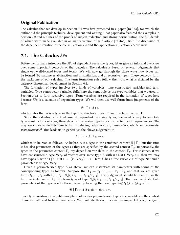
7.1. The Calculus λPµ
Original PublicationThe calculus that we develop in Section 7.1 was first presented in a paper [BG16a], for which theauthor did the principle technical development and writing. That paper also featured the examples inSection 7.2 and outlines of the proofs of subject reduction and strong normalisation, the full detailsof which were made available in an ArXiv version of said article [BG16c]. Both the discussion ofthe dependent iteration principle in Section 7.4 and the application in Section 7.5 are new.
7.1. The Calculus λPµBefore we formally introduce the λPµ of dependent recursive types, let us give an informal overviewover some important concepts of that calculus. The calculus is based on several judgements thatsingle out well-formed types and terms. We will now go through the three ways how types canbe formed: by parameter abstraction and instantiation, and as recursive types. These concepts formthe backbone of our calculus. The term formation rules follow then just what is dictated by thecategory theoretical development in Section 6.2.
The formation of types involves two kinds of variables: type constructor variables and termvariables. Type constructor variables fulfil here the same role as the type variables that we used inSection 3.1.1 to form recursive types. Term variables are required in the formation of types herebecause λPµ is a calculus of dependent types. We will then use well-formedness judgements of theform
Θ | Γ ⊢ A : ∗,which states that A is a type in the type constructor context Θ and the term context Γ.
Since the calculus is centred around dependent recursive types, we need a way to annotatetype constructor variables, through which recursive types are constructed, with dependencies. Theway we chose to do this here is by introducing, what we call, parameter contexts and parameterinstantiations.61 This leads us to generalise the above judgement to
Θ | Γ1 ⊢ A : Γ2 _ ∗,which is to be read as follows. As before, A is a type in the combined context Θ | Γ1, but this timeit has also parameters of the types as they are specified by the second context Γ2. Importantly, thetypes in the parameter context Γ2 my depend on variables in the context Γ1. For instance, if wehave constructed a type VecB of vectors over some type B with n : Nat ⊢ VecB : ∗, then we mayhave types C with Θ | n : Nat ⊢ C : (x : VecB) _ ∗. Here, C has a free variable n of type Nat and aparameter x of type VecB .
Given a parameterised type A as above, we can instantiate its parameters with terms of thecorresponding types as follows. Suppose that Γ2 = x1 : B1, . . . ,xn : Bn and that we are giventerms t1, . . . , tn with Γ1 ⊢ tk : Bk [t1/x1, . . . , tk−1/xk−1]. This judgement should be read as: in theterm variable context Γ1, the term tk is of type Bk [t1/x1, . . . , tk−1/xk−1]. Then we can instantiateparameters of the type A with these terms by forming the new type A@ t1 @ · · ·@ tn with
Θ | Γ1 ⊢ A@ t1 @ · · ·@ tn : ∗.
Since type constructor variables are placeholders for parameterised types, the variables in the contextΘ are also allowed to have parameters. We illustrate this with a small example. Let VecB be again
225
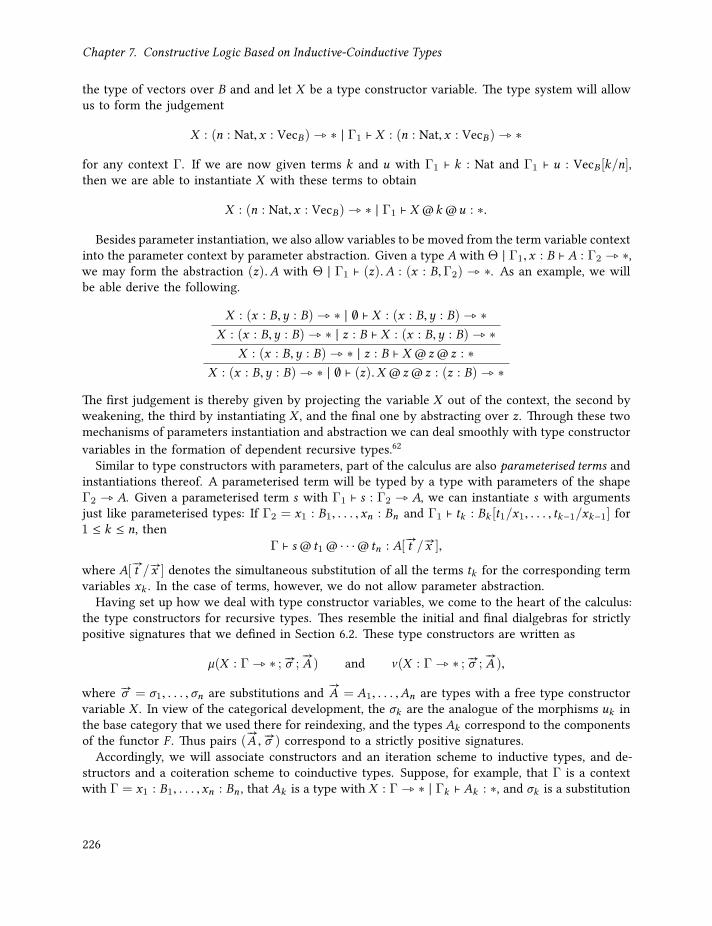
Chapter 7. Constructive Logic Based on Inductive-Coinductive Types
the type of vectors over B and and let X be a type constructor variable. The type system will allowus to form the judgement
X : (n : Nat,x : VecB) _ ∗ | Γ1 ⊢ X : (n : Nat,x : VecB) _ ∗for any context Γ. If we are now given terms k and u with Γ1 ⊢ k : Nat and Γ1 ⊢ u : VecB [k/n],then we are able to instantiate X with these terms to obtain
X : (n : Nat,x : VecB) _ ∗ | Γ1 ⊢ X @k @u : ∗.
Besides parameter instantiation, we also allow variables to be moved from the term variable contextinto the parameter context by parameter abstraction. Given a type A with Θ | Γ1,x : B ⊢ A : Γ2 _ ∗,we may form the abstraction (z).A with Θ | Γ1 ⊢ (z).A : (x : B,Γ2) _ ∗. As an example, we willbe able derive the following.
X : (x : B,y : B) _ ∗ | ∅ ⊢ X : (x : B,y : B) _ ∗X : (x : B,y : B) _ ∗ | z : B ⊢ X : (x : B,y : B) _ ∗
X : (x : B,y : B) _ ∗ | z : B ⊢ X @ z@ z : ∗X : (x : B,y : B) _ ∗ | ∅ ⊢ (z).X @ z@ z : (z : B) _ ∗
The first judgement is thereby given by projecting the variable X out of the context, the second byweakening, the third by instantiating X , and the final one by abstracting over z. Through these twomechanisms of parameters instantiation and abstraction we can deal smoothly with type constructorvariables in the formation of dependent recursive types.62
Similar to type constructors with parameters, part of the calculus are also parameterised terms andinstantiations thereof. A parameterised term will be typed by a type with parameters of the shapeΓ2 _ A. Given a parameterised term s with Γ1 ⊢ s : Γ2 _ A, we can instantiate s with argumentsjust like parameterised types: If Γ2 = x1 : B1, . . . ,xn : Bn and Γ1 ⊢ tk : Bk [t1/x1, . . . , tk−1/xk−1] for1 ≤ k ≤ n, then
Γ ⊢ s @ t1 @ · · ·@ tn : A[#—t / #—x ],
where A[ #—t / #—x ] denotes the simultaneous substitution of all the terms tk for the corresponding term
variables xk . In the case of terms, however, we do not allow parameter abstraction.Having set up how we deal with type constructor variables, we come to the heart of the calculus:
the type constructors for recursive types. Thes resemble the initial and final dialgebras for strictlypositive signatures that we defined in Section 6.2. These type constructors are written as
µ(X : Γ _ ∗ ; #—σ ;#—A ) and ν(X : Γ _ ∗ ; #—σ ;
#—A ),
where #—σ = σ1, . . . ,σn are substitutions and #—A = A1, . . . ,An are types with a free type constructor
variable X . In view of the categorical development, the σk are the analogue of the morphisms uk inthe base category that we used there for reindexing, and the types Ak correspond to the componentsof the functor F . Thus pairs ( #—
A , #—σ ) correspond to a strictly positive signatures.Accordingly, we will associate constructors and an iteration scheme to inductive types, and de-
structors and a coiteration scheme to coinductive types. Suppose, for example, that Γ is a contextwith Γ = x1 : B1, . . . ,xn : Bn , that Ak is a type with X : Γ _ ∗ | Γk ⊢ Ak : ∗, and σk is a substitution
226

7.1. The Calculus λPµ
with σk = (t1, . . . , tn). The kth constructor of µ(X : Γ _ ∗ ; #—σ ;#—A ) is then denoted by αk and has
the following type, where we use the shorthand µ = µ(X : Γ _ ∗ ; #—σ ;#—A ).
⊢ αk : (Γk , z : Ak [µ/X ]) _ (µ@ t1 @ · · ·@ tm) .
The constructor αk can now be instantiated according to the parameter context: Suppose, forsimplicity, that Γk = y : C for some type C that does not depend on X and that we are given a termΓ ⊢ s : C . For a recursive argument Γ ⊢ u : Ak [µ/X ][s/y], we obtain thus
Γ ⊢ αk @ s @u : (µ@ t1 @ · · ·@ tm)[s/y].
The rest of the type and term constructors are the standard structural rules, like weakening,one would expect. It should be noted that there is a strong similarity in the use of destructorsfor coinductive types to λµν . Moreover, the definition scheme for generalised abstract data typesin [HF11] describes the same inductive types. We will discuss this further in Section 7.6.
7.1.1. Raw SyntaxWe now formally introduce the syntax of the calculus λPµ. The first step is to give, what we callhere, its raw syntax. This syntax has only one syntactic class for types and terms, which is givenby the syntactic objects M and N in the following context free grammar. Part of the grammar arealso type and term variable contexts, denoted by Θ and Γ, respectively, and substitutions σ .
Definition 7.1.1. Let Var and TyVar be two disjoint, countably infinite sets of term variables andtype constructor variables. Term variables will be denoted by x ,y, z, . . . , whereas type constructorvariables are denoted by capital letters X ,Y ,Z , . . . . The raw contexts, substitutions and terms aregiven by the following grammar.
ΓF ∅ | Γ,x : M x ∈ VarΘF ∅ | Θ,X : Γ _ ∗σ F () | (σ ,M)
M,N F ⊤ | ⟨ ⟩ | x ∈ Var | M @N | (x).M | X ∈ TyVar | ρ(X : Γ _ ∗ ; #—σ ;#—M ), ρ ∈ µ,ν
| α µ(X :Γ_∗ ; #—σ ;#—A )
k | ξ ν (X :Γ_∗ ; #—σ ;#—A )
k , k ∈ N
| iterµ(X :Γ_∗ ; #—σ ;#—M ) # —
(Γk ,yk .Nk )
| coiterν (X :Γ_∗ ; #—σ ;#—M ) # —
(Γk ,yk .Nk )
To disambiguate raw terms, we use the the convention that instantiation, that is the operator @,binds to the left, and that abstraction binds from the dot all the way to the right.
Let us explain the intention of the raw terms that we have not covered in the introduction above.In the calculus, we have an explicit type ⊤ with a single element ⟨ ⟩, thereby resembling a singletonset. We need this type to form closed terms, as we will explain further in Example 7.2.1. Theterm ξk is the destructor for coinductive types, analogous to the destructor for the greatest fixedpoint types in Section 3.1. Correspondingly, terms of the form coiterν (X :Γ_∗ ; #—σ ;
#—M )
# —
(Γk ,yk .Nk ) are
227

Chapter 7. Constructive Logic Based on Inductive-Coinductive Types
instances of the coiteration scheme for the coinductive type ν(X : Γ _ ∗ ; #—σ ;#—M ). The role of the
terms Nk and the binding construct (Γk ,yk ).Nk will become clearer once we introduce the typingrules for well-formed terms. Thus, we postpone the explanation of these to Section 7.1.4. Dually,iterµ(X :Γ_∗ ; #—σ ;
#—M )
# —
(Γk ,yk .Nk ) is an instance of the iteration scheme for inductive types.The type annotations on the constructors, destructors, and the iteration and coiteration schemes
are necessary in the definition of the reduction relation and typing rules that we give later. However,whenever the annotated types are clear from the context, then we will usually leave them out.
7.1.2. Pre-Types and Pre-TermsThe next step is to separate the raw terms from Section 7.1.1 into, what we call here, pre-typesand pre-terms. This is an intermediate step towards the definition of the typing rules, which hasa two-fold purpose. First of all, the definition of the typing rules of the calculus λPµ require areduction relation on terms. However, we cannot produce such a reduction relation for the rawsyntax because essential to the definition of this relation is an action of types on terms, just like forthe reduction relation of λµν in Section 3.1.2. Such an action on terms is not definable for the wholeraw syntax though. Thus, we are lead to single out syntactic objects that allow us to define an actionon terms for them. These are the pre-types that we are going to define in this section. The secondneed for pre-types and pre-terms arises in the proof of strong normalisation for λPµ. This proof isbased on the construction of a syntactic model in terms of so-called saturated sets. Usually, such asyntactic model is constructed from raw terms because the typing rules get in the way otherwise.But since we can define the reduction relation only on pre-terms, we also use pre-terms as a sweetspot in between raw and typed terms in the strong normalisation proof.
The major difference between pre-types and pre-terms, and the (well-formed) types and terms inSection 7.1.4 is that that pre-terms only get a single placeholder type assigned. This placeholder typeis denoted by an empty box . Having only a placeholder type breaks the dependency betweenthe reduction relation and rules for pre-terms. Such a dependency occurs because among the rulesfor terms is a so-called conversion rule, which allows computations (reduction steps) during type-checking. Instead, we define first pre-terms and pre-types, for which we can define in a second stepthe reduction relation.
Pre-types and pre-terms are defined through the following two judgements.
Θ | Γ1 ⊢pre A : Γ2 _ ∗ and Γ1 ⊢pre t : Γ2 _ .The first judgement expresses that A is a pre-type in the type context Θ, the term context Γ1 andhas the parameter context Γ2. Pre-terms are given by the second judgement, where the contexts Γ1
and Γ2 play the same role, but it should be noted that the type of t is just the placeholder .We will now just give the rules for pre-types and -terms without further commenting on them,
since they are essentially the same as the rules in Section 7.1.4. The only difference is that the typesof terms are erased and that there is no conversion rule for pre-terms. Moreover, the pre-types and-terms are only a technical tool to establish the reduction relation in Definition 7.1.6 and for thestrong normalisation proof. Thus, the reader is advised to skip ahead and read the explanation ofthe reduction relation below and of the well-formedness rules in Section 7.1.4 first. The definitionof pre-terms and pre-types is mostly here for completeness. However, due to the technical difficulty,their definition and that of the reduction relation below have been formalised in Agda [Bas18b].
228
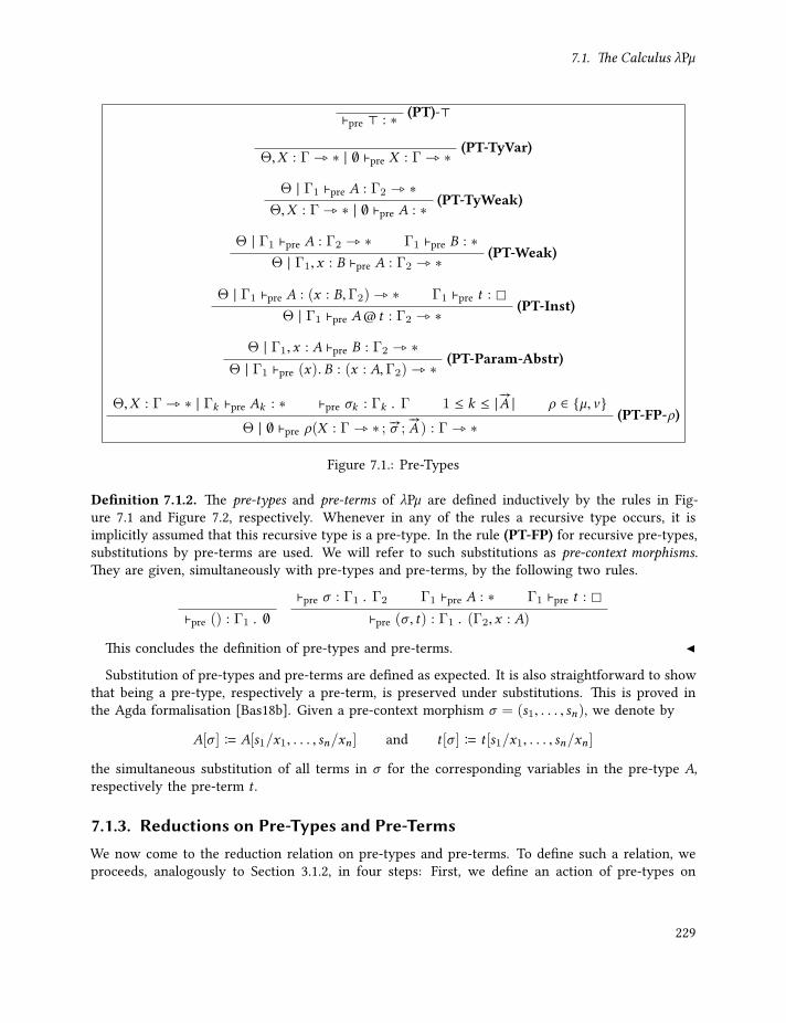
7.1. The Calculus λPµ
(PT)-⊤⊢pre ⊤ : ∗
(PT-TyVar)Θ,X : Γ _ ∗ | ∅ ⊢pre X : Γ _ ∗
Θ | Γ1 ⊢pre A : Γ2 _ ∗(PT-TyWeak)
Θ,X : Γ _ ∗ | ∅ ⊢pre A : ∗
Θ | Γ1 ⊢pre A : Γ2 _ ∗ Γ1 ⊢pre B : ∗(PT-Weak)
Θ | Γ1,x : B ⊢pre A : Γ2 _ ∗Θ | Γ1 ⊢pre A : (x : B,Γ2) _ ∗ Γ1 ⊢pre t :
(PT-Inst)Θ | Γ1 ⊢pre A@ t : Γ2 _ ∗
Θ | Γ1,x : A ⊢pre B : Γ2 _ ∗(PT-Param-Abstr)
Θ | Γ1 ⊢pre (x). B : (x : A,Γ2) _ ∗Θ,X : Γ _ ∗ | Γk ⊢pre Ak : ∗ ⊢pre σk : Γk ▷ Γ 1 ≤ k ≤ | #—A | ρ ∈ µ,ν
(PT-FP-ρ)Θ | ∅ ⊢pre ρ(X : Γ _ ∗ ; #—σ ;
#—A ) : Γ _ ∗
Figure 7.1.: Pre-Types
Definition 7.1.2. The pre-types and pre-terms of λPµ are defined inductively by the rules in Fig-ure 7.1 and Figure 7.2, respectively. Whenever in any of the rules a recursive type occurs, it isimplicitly assumed that this recursive type is a pre-type. In the rule (PT-FP) for recursive pre-types,substitutions by pre-terms are used. We will refer to such substitutions as pre-context morphisms.They are given, simultaneously with pre-types and pre-terms, by the following two rules.
⊢pre () : Γ1 ▷ ∅⊢pre σ : Γ1 ▷ Γ2 Γ1 ⊢pre A : ∗ Γ1 ⊢pre t :
⊢pre (σ , t) : Γ1 ▷ (Γ2,x : A)
This concludes the definition of pre-types and pre-terms.
Substitution of pre-types and pre-terms are defined as expected. It is also straightforward to showthat being a pre-type, respectively a pre-term, is preserved under substitutions. This is proved inthe Agda formalisation [Bas18b]. Given a pre-context morphism σ = (s1, . . . , sn), we denote by
A[σ ] B A[s1/x1, . . . , sn/xn ] and t [σ ] B t [s1/x1, . . . , sn/xn ]
the simultaneous substitution of all terms in σ for the corresponding variables in the pre-type A,respectively the pre-term t .
7.1.3. Reductions on Pre-Types and Pre-TermsWe now come to the reduction relation on pre-types and pre-terms. To define such a relation, weproceeds, analogously to Section 3.1.2, in four steps: First, we define an action of pre-types on
229

Chapter 7. Constructive Logic Based on Inductive-Coinductive Types
(PO-⊤-I)⊢pre ⟨ ⟩ : Γ1 ⊢pre t : (x : A,Γ2) _ Γ1 ⊢pre s : (PO-Inst)
Γ1 ⊢pre t @ s : Γ2 _ x ∈ Var Γ ⊢pre A : ∗
(PO-Proj)Γ,x : A ⊢pre x : Γ ⊢pre A : ∗ Γ1 ⊢pre t : Γ2 _
(PO-Weak)Γ1,x : A ⊢pre t : Γ2 _
1 ≤ k ≤ | #—A | (PO-Ind-I)⊢pre α µ(X :Γ_∗ ; #—σ ;
#—A )
k : (Γk ,y : Ak [µ/X ]) _ 1 ≤ k ≤ | #—A | (PO-Coind-E)
⊢pre ξ ν (X :Γ_∗ ; #—σ ;#—A )
k : (Γk ,y : ν @σk ) _ ∆ ⊢pre C : Γ _ ∗ ∀1 ≤ k ≤ | #—A |.
(∆,Γk ,yk : (C @σk ) ⊢pre дk : )
(PO-Ind-E)∆ ⊢pre iterµ(X :Γ_∗ ; #—σ ;
#—A )
# —
(Γk ,yk .Nk ) : (Γ,y : µ@idΓ) _ ∆ ⊢pre C : Γ _ ∗ ∀1 ≤ k ≤ | #—A |.
(∆,Γk ,yk : (C @σk ) ⊢pre дk : )
(PO-Coind-I)∆ ⊢pre coiterν (X :Γ_∗ ; #—σ ;
#—A )
# —
(Γk ,yk .Nk ) : (Γ,y : C @idΓ) _ Figure 7.2.: Pre-Terms
pre-terms. Then we use this action to define a simple contraction relation. From this contractionrelation we obtain, as the third step, a reduction relation by taking its compatible closure. Finally,we use the resulting reduction relation on pre-terms to define a reduction on pre-types.
For convenience, let us introduce some notation for dealing with pre-context morphisms. Thesenotations make it also easier to relate the present development to the category theoretical approachin Section 6.2.Notation 7.1.3. First, for Γ = x1 : A1, . . . ,xn : An we define the identity (pre-)context morphismidΓ by idΓ B (x1, . . . ,xn). Second, given a type A with Θ | Γ1 ⊢pre A : Γ _ ∗ and a pre-contextmorphism σ with ⊢pre σ : Γ1 ▷ Γ and σ = (t1, . . . , tn), we denote by A@σ the instantiationA@ t1 @ · · ·@ tn . Finally, we will need to compose pre-context morphisms later. This compositionis given for pre-context morphisms Γ3
σ▷ Γ2
τ▷ Γ by
τ • σ B (τ1[σ ], . . . ,τn [σ ]), (7.1)
where τk [σ ] denotes the substitution of σ in all terms in τk .
Since we will frequently deal with parameter abstractions of many variables at the same time, itis worth to also introduce some notation concerning multi-variable abstractions.Notation 7.1.4. Let us agree on the following notations for parameter abstraction. Given a contextΓ = x1 : A1, . . . ,xn : An and a pre-type Θ | Γ ⊢pre B : ∗, we denote the full abstraction of B by(Γ). B B (x1). · · · (xn). B, which gives us
Θ | ∅ ⊢pre (Γ). B : Γ _ ∗.230
7.1. The Calculus λPµ
Moreover, if we are given a sequence #—B of such types, that is, if Θ | Γi ⊢pre Bi : ∗ for each Bi in
that sequence, we denote by# —
(Γi ). B the sequence of types that arises by fully abstracting each typeBi separately.
Having introduced all this notation, we can now define the action A of a pre-type A on pre-typesand -terms. Suppose that A andU are pre-types with X : Γ _ ∗ | Γ1 ⊢pre A : Γ2 _ ∗ and Γ ⊢pre U : ∗.Then the action of A on U is given by
A(U ) = A[(Γ).U /X ]@idΓ2.
On terms, we will define A so that the following rule holds.
X : Γ _ ∗ | Γ1 ⊢pre A : Γ2 _ ∗ Γ,x : U ⊢pre t : Γ1,Γ2,y : A(U ) ⊢pre A(t) :
This action of pre-types is defined analogously to that of types on terms in the simply typed casein Section 3.1.2. As such, it follows in the case of recursive types the definition of functors fromparameterised initial and final dialgebras in Section 6.2.2. In fact, A has the type of a functor thatturns types in context Γ into types in the context Γ1,Γ2. That will become clearer once we introducewell-formed types and terms in Section 7.1.4 and prove subject reduction in Section 7.3.2.
In the following definition of the action of pre-types, we need to generalise the above rules toan arbitrary number of free type constructor variables in A. That means that, instead of assumingX : Γ _ ∗ | Γ1 ⊢pre A : Γ2 _ ∗, we have Θ | ∆1 ⊢pre A : ∆2 _ ∗ for an arbitrary type context Θ.
Definition 7.1.5. Let Θ | ∆1 ⊢pre A : ∆2 _ ∗ be a pre-type with Θ = X1 : Γ1 _ ∗, . . . ,Xn : Γn _ ∗,#—U and #—
V be sequences of pre-types with Γi ⊢pre Ui : ∗ and Γi ⊢pre Vi : ∗ for all 1 ≤ i ≤ n. The actionof A on the sequence #—
U of types is given by
A(#—U ) B A[
# —
(Γi ).U /#—X ]@id∆2
.
Note that we then have that Θ | ∆1,∆2 ⊢pre A(#—U ) : ∗.
For a sequence #—t of pre-terms with Γi ,x : Ui ⊢pre t : for all 1 ≤ i ≤ n, we define the action of
A on #—t , denoted by A(
#—t ), so that the following rule holds.
Θ | ∆1 ⊢pre C : ∆2 _ ∗ ∀1 ≤ i ≤ n. Γi ,x : Ui ⊢pre ti : ∆1,∆2,y : C(
#—U ) ⊢pre C( #—
t ) : If n = 0, we simply put A(ε) = y, which also covers the case (PT-⊤). If n > 0, we define A(
#—t )
231
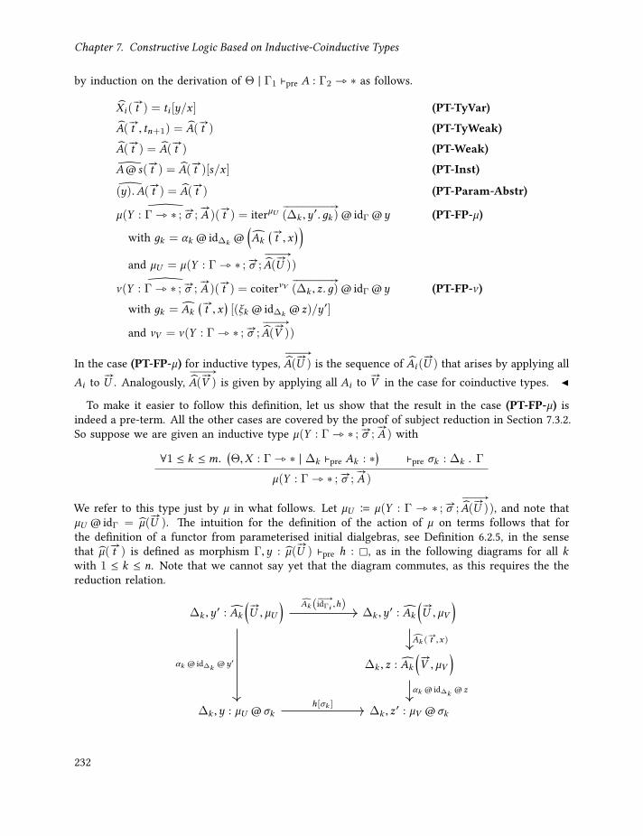
Chapter 7. Constructive Logic Based on Inductive-Coinductive Types
by induction on the derivation of Θ | Γ1 ⊢pre A : Γ2 _ ∗ as follows.
Xi (#—t ) = ti [y/x ] (PT-TyVar)
A(#—t , tn+1) = A(
#—t ) (PT-TyWeak)
A(#—t ) = A(
#—t ) (PT-Weak)A@ s(
#—t ) = A(
#—t )[s/x ] (PT-Inst)(y).A( #—
t ) = A(#—t ) (PT-Param-Abstr)µ(Y : Γ _ ∗ ; #—σ ;
#—A )(
#—t ) = iterµU
# —
(∆k ,y′.дk )@idΓ @y (PT-FP-µ)
with дk = αk @id∆k @(Ak
( #—t ,x
) )and µU = µ(Y : Γ _ ∗ ; #—σ ;
# —
A(#—U ))ν(Y : Γ _ ∗ ; #—σ ;
#—A )(
#—t ) = coiterνV
# —
(∆k , z.д)@idΓ @y (PT-FP-ν )
with дk = Ak( #—t ,x
)[(ξk @id∆k @ z)/y ′]
and νV = ν(Y : Γ _ ∗ ; #—σ ;# —
A(#—V ))
In the case (PT-FP-µ) for inductive types,# —
A(#—U ) is the sequence of Ai (
#—U ) that arises by applying all
Ai to #—U . Analogously,
# —
A(#—V ) is given by applying all Ai to #—
V in the case for coinductive types.
To make it easier to follow this definition, let us show that the result in the case (PT-FP-µ) isindeed a pre-term. All the other cases are covered by the proof of subject reduction in Section 7.3.2.So suppose we are given an inductive type µ(Y : Γ _ ∗ ; #—σ ;
#—A ) with
∀1 ≤ k ≤ m.(Θ,X : Γ _ ∗ | ∆k ⊢pre Ak : ∗
)⊢pre σk : ∆k ▷ Γ
µ(Y : Γ _ ∗ ; #—σ ;#—A )
We refer to this type just by µ in what follows. Let µU B µ(Y : Γ _ ∗ ; #—σ ;# —
A(#—U )), and note that
µU @idΓ = µ(#—U ). The intuition for the definition of the action of µ on terms follows that for
the definition of a functor from parameterised initial dialgebras, see Definition 6.2.5, in the sensethat µ( #—
t ) is defined as morphism Γ,y : µ(#—U ) ⊢pre h : , as in the following diagrams for all k
with 1 ≤ k ≤ n. Note that we cannot say yet that the diagram commutes, as this requires the thereduction relation.
∆k ,y′ : Ak
(#—U , µU
)∆k ,y
′ : Ak
(#—U , µV
)∆k , z : Ak
(#—V , µV
)∆k ,y : µU @σk ∆k , z
′ : µV @σk
Ak(# —idΓi ,h)
αk @id∆k @y′
Ak (#—t ,x)
αk @id∆k @ z
h[σk ]
232

7.1. The Calculus λPµ
iter# —
(Γk ,yk .дk )@ (σk • τ )@ (αk @τ @u) ≻ дk[Ak (iter
# —
(Γk ,yk .дk )@idΓ @x)/yk
][τ ,u]
ξk @τ @ (coiter# —
(Γk ,yk .дk )@ (σk • τ )@u) ≻ Ak
(coiter
# —
(Γk ,yk .дk )@idΓ @x)[дk/y][τ ,u]
Figure 7.3.: Contraction of Terms.
In Definition 7.1.5, the pre-term h was given by defining
дk = αk @id∆k @(Ak
( #—t ,x
) )h = iterµU
# —
(∆k ,y′.дk )@idΓ @y.
Note that дk = (αk @id∆k @ z)[(Ak
( #—t ,x
) )/z], which is the right-hand side of the above diagram.
Let us now derive that all the дk and h are correct pre-terms. First of all, we obtain from theinduction hypothesis in the definition of the pre-type action the following derivation.
Θ,X : Γ _ ∗ | ∆k ⊢pre Ak : ∗ ∀1 ≤ i ≤ n.(Γi ,x : Ui ⊢pre t : )
Γ,x : µ(#—V ) ⊢pre x :
∆k ,y′ : Ak (
#—U , µ(
#—V )) ⊢pre Ak (
#—t ,x) :
By the typing rules for the constructors of the inductive type µU , we also have the following.
∆k , z : Ak (#—U , µU ) ⊢pre z :
∆k , z : Ak (#—U , µU ) ⊢pre αk @id∆k @ z :
Putting these together, we have
∀1 ≤ i ≤ n.(Γi ,x : Ui ⊢pre t : )
∀1 ≤ k ≤ m.(∆k ,y
′ : Ak (#—U , µ(
#—V )) ⊢pre дk : )
⊢pre iterµU# —
(∆k ,y.дk ) : (Γ,y : µ(#—U )) _
Γ,y : µ(#—U ) ⊢pre h :
This shows that µ( #—t ) = h is indeed a pre-term in the expected context.
We now come to the definition of the reduction relations on pre-terms and pre-types. Analogouslyto the development in Section 3.1.2, we define the reduction relation on pre-terms by first givinga contraction relation, which carries out single-step computations, and then taking the compatibleclosure of this contraction relation is reduction relation. The reduction relation on pre-types reducesthen parameters by means of the reduction relation on pre-terms. Moreover, it performs β-reductionfor instantiations.
So let us start by providing the reduction on pre-terms by appealing to the action of pre-types.
Definition 7.1.6. The reduction relation of λPµ −→ on pre-terms is defined as compatible closure63of the contraction relation of λPµ ≻ given in Figure 7.3. We introduce in the definition of contractiona fresh variable x , for which we immediately substitute (either u or дk ). This is necessary for theuse of the action of types on terms, see Definition 7.1.5.
233

Chapter 7. Constructive Logic Based on Inductive-Coinductive Types
On terms, the reduction relation for a destructor-coiterator pair essentially emulates the ho-momorphism diagram for coinductive extensions. So suppose we are given a coinductive typeν = ν(Y : Γ _ ∗ ; #—σ ;
#—A ) with Γk ⊢pre Ak : ∗ and a pre-type C with ⊢pre C : Γ _ ∗. Then the
contraction relation acts as in the following diagram, where composition is given by substitution.
Γk ,xk : C @σk Γk ,y : ν @σk
Γk ,y : Ak [C/X ] Γk , z : Ak [ν/X ]
coiter # —
(Γk ,y . дk )@σk @ x
дk ξk @idΓk @y≺
Ak (coiter# —
(Γk ,y . д)@σk @ x)
To be precise, this means that we have
(ξk @idΓk @y)[coiter
# —
(Γk ,y.дk )@σk @x/y]= ξk @idΓk @
(coiter
# —
(Γk ,y.дk )@σk @x)y
≻ Ak (coiter# —
(Γk ,y.д)@σk @x)[дk/y].
The reduction relation for a iterator-constructor pair emulates the dual of this diagram for homo-morphisms out of initial dialgebras.
From the reduction relation on pre-terms, we can now define reductions on pre-types.
Definition 7.1.7. The reduction relation on pre-types consists of two types of reductions: First,β-reduction for parameter instantiations is given by parameter reduction64
((x).A)@ t −→p A[t/x ].
Second, we lift the reduction relation on pre-terms to pre-types by taking the compatible closure ofreduction of parameters, which is given by
t −→ t ′
A@ t −→ A@ t ′(7.2)
We combine these relations into one reduction relation on pre-types:
−→T B −→p ∪ −→.
One-step conversion of pre-types is then given by
A←→T B ⇐⇒ A −→T B or B −→T A.
This concludes the definition of reductions on pre-types and -terms. So we can finally come tothe definition well-formed types and terms.
7.1.4. Well-Formed Types and TermsThe goal of this section is carve out the well-formed types and terms of the calculus λPµ fromthe pre-terms and pre-types that we defined in the last section. We will do this through severaljudgements, each of which has its own set of derivations rules. It is understood that the derivabilityof these judgments is defined by simultaneous induction. So, Definitions 7.1.8, 7.1.9, 7.1.10 and 7.1.11should be seen as one simultaneous definition. The judgements we are going to use are are thefollowing.
234

7.1. The Calculus λPµ
• ⊢ Θ TyCtx — The type constructor variable context Θ is well-formed.
• ⊢ Γ Ctx — The term variable context Γ is well-formed.
• σ : Γ1 ▷ Γ2 – The context morphism σ is a well-formed substitution for Γ2 with terms incontext Γ1.
• Θ | Γ1 ⊢ A : Γ2 _ ∗ — The type constructor A is well-formed in the combined contextΘ | Γ1 and can be instantiated with terms according to the parameter context Γ2, where it isimplicitly assumed that Θ, Γ1 and Γ2 are well-formed.
• Γ1 ⊢ t : Γ2 _ A — The term t is well-formed in the term variable context Γ1 and, afterinstantiating it with arguments according to parameter context Γ2, is of type A with thearguments substituted into A.
Definition 7.1.8. The judgements for singling out well-formed contexts (type variable contexts andterm variable contexts) are given by the following rules.
⊢ ∅ TyCtx⊢ Θ TyCtx ⊢ Γ Ctx⊢ Θ,X : Γ _ ∗ TyCtx ⊢ ∅ Ctx
∅ | Γ ⊢ A : ∗⊢ Γ,x : A Ctx
It is important to note that whenever a term variable declaration is added into the context, itstype is not allowed to have any free type constructor variables, which ensures that all types arestrictly positive. For example, we are not allowed to form the term context Γ = x : X in which Xoccurs freely. This prevents us, as we will see in Ex. 7.2.4, from forming function spaces X → A.
Definition 7.1.9 (Context Morphism). We introduce the notion of context morphisms as a shorthandnotation for typed substitutions. Let Γ1 and Γ2 be contexts. A context morphism σ : Γ1 ▷ Γ2 is givenby the following two rules.
() : Γ1 ▷ ∅σ : Γ1 ▷ Γ2 Γ1 ⊢ t : A[σ ]
(σ , t) : Γ1 ▷ (Γ2,x : A)
where ∅ | Γ2 ⊢ A : ∗, and A[σ ] denotes the simultaneous substitution of the terms in σ for thecorresponding variables, which is often also denoted by A[σ ] = A[σ/ #—x ].
Definition 7.1.10 (Well-formed Type Constructor of λPµ). The judgement for type constructors isgiven inductively by the rules in Figure 7.4, where it is understood that all involved contexts arewell-formed. where in the (FP-Ty)-rule #—σ and #—
A are assumed to have the same length | #—A |.
Note that type constructor variables come with a parameter context. This context determines theparameters of an initial/final dialgebra, which essentially bundle the local context, the domain andthe codomain of their constructors respectively destructors. In other words, the types implementprecisely the closure rules for µP-complete categories.
This brings us finally to the rules for well-formed terms.
Definition 7.1.11 (Well-formed Terms of λPµ). The judgement for terms is given by the rules inFig. 7.5. To improve readability, we use the shorthand ρ = ρ(X : Γ _ ∗ ; #—σ ;
#—A ), ρ ∈ µ,ν , and
implicitly assume all involved types and contexts are well-formed.
235

Chapter 7. Constructive Logic Based on Inductive-Coinductive Types
(⊤-I)⊢ ⊤ : ∗
⊢ Θ TyCtx ⊢ Γ Ctx(TyVar-I)
Θ,X : Γ _ ∗ | ∅ ⊢ X : Γ _ ∗Θ | Γ1 ⊢ A : Γ2 _ ∗ ⊢ Γ Ctx (TyVar-Weak)Θ,X : Γ _ ∗ | Γ1 ⊢ A : Γ2 _ ∗Θ | Γ1 ⊢ A : Γ2 _ ∗ Γ1 ⊢ B : ∗ (Ty-Weak)
Θ | Γ1,x : B ⊢ A : Γ2 _ ∗Θ | Γ1 ⊢ A : (x : B,Γ2) _ ∗ Γ1 ⊢ t : B (Ty-Inst)
Θ | Γ1 ⊢ A@ t : Γ2[t/x ] _ ∗Θ | Γ1,x : A ⊢ B : Γ2 _ ∗ (Param-Abstr)
Θ | Γ1 ⊢ (x). B : (x : A,Γ2) _ ∗∀1 ≤ k ≤
#—A
. σk : Γk ▷ Γ Θ,X : Γ _ ∗ | Γk ⊢ Ak : ∗ ρ ∈ µ,ν (FP-Ty-ρ)
Θ | ∅ ⊢ ρ(X : Γ _ ∗ ; #—σ ;#—A ) : Γ _ ∗
Figure 7.4.: Judgements for the well-formed types of λPµ
We will often leave out the type information in the superscript of constructors and destructors. Thedomain of a constructor α µ(X :Γ_∗ ; #—σ ;
#—A )
k is determined by Ak and its codomain by the instantiationσk . Dually, the domain of a destructor ξk is given by the instantiation σk and its codomain byAk . It is important to note in that both the iteration and coiteration schemes variable binding isintroduced: Given terms дk with ∆,Γk ,yk : Ak [C/X ] ⊢ дk : C @σk , the iterator iter
# —
(Γk ,yk .дk )binds the variables in Γk and the variable yk of each дk . For instance, this will give us the variablebinding that happens in λ-abstraction, see Example 7.2.4.
This concludes the definition of our proposed calculus λPµ. Note that there are no primitive typeconstructors for →-, Π- or ∃-types, all of these are, together with the corresponding introductionand elimination principles, definable in the above calculus, as we will see in the next section.
As the alert reader might have noticed, our calculus does not have dependent recursion andcorecursion, that is, the type C in (Ind-E) and (Coind-I) cannot depend on elements of the cor-responding recursive type. This clearly makes the calculus weaker than if we had the dependentversion: In the case of inductive types we do not have an induction principle, cf. Example 7.2.6. Wewill come back to this issue in Section 7.4. For coinductive types, on the other hand, one cannoteven formulate a dependent version of (Coind-I), rather one would expect a coinduction rule thatturns a bisimulation into an equality proof. This would imply that we have an extensional functionspace, see Example 7.2.4. How to possibly add such a bisimulation proof principle will be discussedin the future work in Section 7.6.
236

7.2. Examples
(⊤-I)⊢ ⟨ ⟩ : ⊤Γ1 ⊢ t : (x : A,Γ2) _ B Γ1 ⊢ s : A (Inst)
Γ1 ⊢ t @ s : Γ2[s/x ] _ B[s/x ]
Γ ⊢ t : A A←→T B (Conv)Γ ⊢ t : B
Γ ⊢ A : ∗ (Proj)Γ,x : A ⊢ x : A
Γ1 ⊢ t : Γ2 _ A Γ1 ⊢ B : ∗ (Weak)Γ1,x : B ⊢ t : Γ2 _ A
⊢ µ(X : Γ _ ∗ ; #—σ ;#—A ) : Γ _ ∗ 1 ≤ k ≤ | #—A |
(Ind-I)⊢ α µ(X :Γ_∗ ; #—σ ;
#—A )
k : (Γk ,y : Ak [µ/X ]) _ µ@σk
⊢ ν(X : Γ _ ∗ ; #—σ ;#—A ) : Γ _ ∗ 1 ≤ k ≤ | #—A |
(Coind-E)⊢ ξ ν (X :Γ_∗ ; #—σ ;
#—A )
k : (Γk ,y : ν @σk ) _ Ak [ν/X ]
∆ ⊢ C : Γ _ ∗ ∆,Γk ,yk : Ak [C/X ] ⊢ дk : (C @σk ) ∀k = 1, . . . , #—A
(Ind-E)
∆ ⊢ iter # —
(Γk ,yk .дk ) : (Γ,y : µ@idΓ) _ C @idΓ
∆ ⊢ C : Γ _ ∗ ∆,Γk ,yk : (C @σk ) ⊢ дk : Ak [C/X ] ∀k = 1, . . . , #—A
(Coind-I)
∆ ⊢ coiter # —
(Γk ,yk .дk ) : (Γ,y : C @idΓ) _ ν @idΓ
Figure 7.5.: Judgements for well-formed terms of λPµ
7.2. ExamplesIn this section, we illustrate the calculus given in Section 7.1 on a variety of examples. We beginwith a few basic ones, then work our way through the encoding of logical operators, and finish withlists indexed by their length (vectors) as an actually recursive type.
Before we go through the examples, let us introduce a notation for sequences of empty contextmorphisms. We denote such a sequence of k empty context morphisms by
εk B ((), . . . , ()).
Given contexts Γ1, . . . ,Γk , we then have that εk is a sequence of context morphisms (Γ1 ▷ ∅, . . . ,Γk ▷∅).
Let us start with one of the most basic types: the singleton type. This first example also gives usthe opportunity to explain the role of the base type ⊤.
Example 7.2.1 (Final Object). We first note that, in principle, we can encode ⊤ as a coinductivetype by 1 B ν(X : ∗ ; ε1;X ):
X : ∗ | ∅ ⊢ X : ∗ ε1 : ∅ ▷ ∅ (FP-Ty)⊢ ν(X : ∗ ; ε1;X ) : ∗
237

Chapter 7. Constructive Logic Based on Inductive-Coinductive Types
This gives us the destructor ξ1 : (x : 1) _ 1 and the inference⊢ C : ∗ y : C ⊢ y : C
(Coind-I)⊢ coiter (y.y) : (y : C) _ 1So the analogue of the categorical concept of the (unique) morphism into a final object is given by!C B coiter (y.y). Note that it is not possible to define a closed term of type 1 directly, rather weonly get one with the help of ⊤ by ⟨ ⟩′ B !⊤@ ⟨ ⟩. Thus, the purpose of ⊤ is to allow the formationof closed terms. Now, these definitions and X (t) = t , see Def. 7.1.5, give us the following reduction.
ξ1 @ ⟨ ⟩′ = ξ1 @ (coiter (y.y)@ ⟨ ⟩)
−→ X (coiter (y.y)@x)[⟨ ⟩/y]
= (coiter (y.y)@x)[y/x ][⟨ ⟩/y]
= coiter (y.y)@ ⟨ ⟩
= ⟨ ⟩′
Hence, ⟨ ⟩′ is the canonical element of 1 with no observable behaviour.
Dual to the final object 1, we can form an initial object.Example 7.2.2. We put 0 B ⊥ B µ(X : ∗ ; ε1;X ), dual to the definition of 1. For a given type C ,we can define the usual elimination principle for falsum by E⊥C B iter (y.y). As expected, we have
Γ ⊢ C : ∗Γ ⊢ E⊥C : (y : ⊥) _ C
Let us now move to more complex type formers, or logical connectives under the propositions-as-types interpretation.Example 7.2.3 (Binary Product and Coproduct). Suppose we are given types Γ ⊢ A1,A2 : ∗, thentheir binary product is fully specified by the two projections and pairing. Thus, we can use thefollowing coinductive type for A1 ×Γ A2.
Γ ⊢ A1 : ∗ Γ ⊢ A2 : ∗Γ ⊢ ν(X : Γ _ ∗ ; (idΓ, idΓ); (A1,A2))@idΓ : ∗
Then the projections are given by πk B ξk @idΓ, and pairing by ⟨t1, t2⟩ B Pt1,t2 @idΓ @ ⟨ ⟩, where weabbreviate Pt1,t2 B coiter ((Γ, _. t1), (Γ, _. t2)). For this definition of pairing, we have the followingexpected typing derivation.
⊢ (Γ).⊤ : Γ _ ∗ Γ ⊢ tk : Ak
Γ, _ : ⊤ ⊢ tk : Ak
⊢ Pt1,t2 : (Γ, _ : ⊤) _ A1 ×Γ A2
Γ ⊢ ⟨t1, t2⟩ : A1 ×Γ A2
This setup gives us the usual reductions for k ∈ 1, 2:πk @ ⟨t1, t2⟩ = ξk @idΓ @ (Pt1,t2 @idΓ @ ⟨ ⟩)
−→ Ak (Pt1,t2 @idΓ @x)[tk/y][(idΓ, ⟨ ⟩)]= y[tk/y][(idΓ, ⟨ ⟩)]= tk ,
238

7.2. Examples
where the third step is given by Ak = y, since Ak does not use type constructor variables,see Def. 7.1.5.
Dually, the binary coproduct of A1 and A2 is given by
A1 +Γ A2 B µ(X : Γ _ ∗ ; (idΓ, idΓ); (A1,A2))@idΓ,
the corresponding injections by κi B αi @idΓ, and we can form the case distinction
κ1 x1 7→ t1 ; κ2 x2 7→ t2 s B iter ((Γ,x . t1), (Γ,x . t2))@ s,
which is subject to the following typing rule.
Γ ⊢ C : ∗ Γ,xk : Ak ⊢ tk : C Γ ⊢ s : A1 +Γ A2
Γ ⊢ κ1 x1 7→ t1 ; κ2 x2 7→ t2 s : C
Moreover, we get the expected reduction:
κ1 x1 7→ t1 ; κ2 x2 7→ t2 (κk @ s) −→ tk [s/xk ].
Thus, we have recovered binary products and coproducts with their introduction and eliminationrules, and the corresponding reduction rules in λPµ. These definitions correspond to our result inTheorem 6.2.11 and the table that follows this theorem.
Next, we show how to recover the dependent function space as coinductive type and dependentsums as inductive types in λPµ. This follows again Theorem 6.2.11.
Example 7.2.4 (Dependent Product, Universal Quantifier). Given types A and B with ⊢ A : ∗ andx : A ⊢ B : ∗, we expect the dependent product of B to be a type with ⊢ Πx : A. B : ∗. This leads usto use ∅ as global context for the dependent product and Γ1 = x : A as local context. Since we have
x : A ⊢ B : ∗(TyVar-Weak)X : ∗ | x : A ⊢ B : ∗ ε1 : Γ1 ▷ ∅ (FP-Ty)
⊢ ν(X : ∗ ; ε1;B) : ∗
we may define Πx : A.B B ν(X : ∗ ; ε1;B). If t is a term with Γ,x : A ⊢ t : B, we get its λ-abstractionby putting λx .t B coiter (x ,u . t)@ ⟨ ⟩ for some fresh variable u. This term is indeed correctly typed:
Γ,x : A ⊢ t : B Γ,x : A ⊢ ⊤ : ∗ (Weak)Γ,x : A,u : ⊤ ⊢ t : B (Coind-I)
Γ ⊢ coiter (x ,u . t) : (u : ⊤) _ Πx : A.B(Inst)
Γ ⊢ λx .t : Πx : A.B
Function application is given by destructor application: s a B ξ1 @a@ s . Since we have thatB[Πx : A.B/X ] = B and (Πx : A.B)[ε1] = Πx : A.B, we can derive the typing rule for application.
Γ ⊢ a : A Γ ⊢ s : Πx : A.BΓ ⊢ s a : B[a/x ]
239
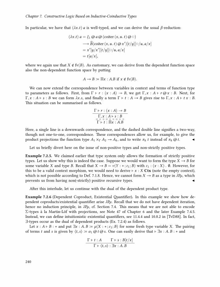
Chapter 7. Constructive Logic Based on Inductive-Coinductive Types
In particular, we have that (λx .t) a is well-typed, and we can derive the usual β-reduction:
(λx .t) a = ξ1 @a@ (coiter (x ,u . t)@ ⟨ ⟩)
−→ B(coiter (x ,u . t)@x ′)[t/y][⟨ ⟩/u,a/x ]
= x ′[y/x ′][t/y][⟨ ⟩/u,a/x ]
= t [a/x ],
where we again use that X < fv(B). As customary, we can derive from the dependent function spacealso the non-dependent function space by putting
A→ B B Πx : A.B if x < fv(B).
We can now extend the correspondence between variables in context and terms of function typeto parameters as follows. First, from Γ ⊢ r : (x : A) _ B, we get Γ,x : A ⊢ r @x : B. Next, forΓ,x : A ⊢ s : B we can form λx .s , and finally a term Γ ⊢ t : A → B gives rise to Γ,x : A ⊢ t x : B.This situation can be summarised as follows.
Γ ⊢ r : (x : A) _ B
Γ,x : A ⊢ s : BΓ ⊢ t : Πx : A.B
Here, a single line is a downwards correspondence, and the dashed double line signifies a two-way,though not one-to-one, correspondence. These correspondences allow us, for example, to give theproduct projections the function type A1 ×Γ A2 → Ak , and to write πk t instead of πk @ t .
Let us briefly divert here on the issue of non-positive types and non-strictly positive types.
Example 7.2.5. We claimed earlier that type system only allows the formation of strictly positivetypes. Let us show why this is indeed the case. Suppose we would want to form the type X → B forsome variable X and type B. Recall that X → B = ν(Y : ∗ ; ε1;B) with ε1 : (x : X ) ▷ ∅. However, forthis to be a valid context morphism, we would need to derive ⊢ x : X Ctx (note the empty context),which is not possible according to Def. 7.1.8. Hence, we cannot form X → B as a type in λPµ, whichprevents us from having non(-strictly) positive recursive types.
After this interlude, let us continue with the dual of the dependent product type.
Example 7.2.6 (Dependent Coproduct, Existential Quantifier). In this example we show how de-pendent coproducts/existential quantifier arise λPµ. Recall that we do not have dependent iteration,hence no induction principle, in λPµ, cf. Section 7.4. This means that we are not able to encodeΣ-types à la Martin-Löf with projections, see Note 47 of Chapter 6 and the later Example 7.4.5.Instead, we can define intuitionistic existential quantifiers, see 11.4.4 and 10.8.2 in [TvD88]. In fact,∃-types occur as the dual of dependent products (Ex. 7.2.4) as follows.
Let x : A ⊢ B : ∗ and put ∃x : A. B B µ(X : ∗ ; ε1;B) for some fresh type variable X . The pairingof terms t and s is given by ⟨t , s⟩ B α1 @ t @ s . One can easily derive that ⊢ ∃x : A. B : ∗ and
Γ ⊢ t : A Γ ⊢ s : B[t/x ]Γ ⊢ ⟨t , s⟩ : ∃x : A. B
240
7.2. Examples
from (Ind-I) and (Inst). Equally easy is also the derivation that the elimination principle forexistential quantifiers, defined by
unpack t as ⟨x ,y⟩ in p B iter (x : A,y : B.p)@ t ,
can be formed by the following rule.
⊢ C : ∗ Γ,x : A,y : B ⊢ p : C Γ ⊢ t : ∃x : A.B
Γ ⊢ unpack t as ⟨x ,y⟩ in p : C
Finally, we get the usual reduction rule
unpack ⟨t , s⟩ as ⟨x ,y⟩ in p −→ p [t/x , s/y ] .
Even though we do not have a strong enough elimination principle for ∃-types to define thesecond projection of pairs, we are still able to define the first projection by
π1 B λz. unpack z as ⟨x ,y⟩ in x .
Indeed, one easily derives that ⊢ π1 : (∃x : A. B)→ A.
Example 7.2.7 (Generalised Dependent Product and Coproduct). From a categorical perspective, itmakes sense to not just consider product and coproducts that bind a variable in a type but also toallow the restriction of terms we allow as values for this variable. We can achieve this by replacingε1 in Ex. 7.2.4 and Ex. 7.2.6 by an arbitrary term x : I ⊢ f : J . This gives us type constructors with
y : J ⊢⨿f A : ∗ and y : J ⊢∏
f A : ∗
that are weakly adjoint⨿
f ⊣ f ∗ ⊣ ∏f , where f ∗ substitutes f . Similarly, propositional equality
arises as left adjoint to contraction δ ∗, where δ : (x : A) ▷ (x : A,y : A) is the diagonal substitutionδ B (x ,x), see Example 7.2.8 below.
Example 7.2.8 (Propositional Equality). In Ex. 7.2.7, we remarked that the propositional equalityarises as left adjoint to the contraction δ ∗, cf. [Jac99, Def. 10.5.1], hence can be represented in λPµ asa generalised dependent coproduct. Let us elaborate this a bit more. First, we represent the equalitytype in λPµ as an inductive type by
EqA(s, t) B µ(X : (x : A,y : A) _ ∗ ;δ ;⊤)@ s @ t ,
where δ : (x : A) ▷ (x : A,y : A) is the diagonal δ = (x ,x). This type has the usual constructor
refl : Πx : A. EqA(x ,x)refl B λx . α1 : (x : A) _ EqA(x ,x)
and the (weak) elimination rule
x : A,y : A ⊢ C : ∗ x : A ⊢ p : C[x/x ,x/y] Γ ⊢ q : EqA(s, t)Γ ⊢ EEq(p,q) : C [s/x , t/y ]
241

Chapter 7. Constructive Logic Based on Inductive-Coinductive Types
where EEq(p,q) B iter (x .p)@ s @ t @q. This is of course not the full J-rule (or path induction)but it is already strong enough to prove, for example, the following replacement (or substitution ortransport) rule that allows us to replace equal terms in types.
Γ,x : A ⊢ P : ∗ Γ ⊢ p : P [s/x ] Γ ⊢ q : EqA(s, t)Γ ⊢ repl(p,q) : P [t/x ]
This can be derived by using P [x/x ]→ P [y/x ] for C and puttingrepl(p,q) B EEq(λr . r ,q) p.
That this term is of the correct type can be seen by the following derivation.
Γ ⊢ λr . r : P [x/x ]→ P [x/x ] Γ ⊢ q : EqA(s, t)Γ ⊢ EEq(λr . r ,q) : P [s/x ]→ P [t/x ] Γ ⊢ p : P [s/x ]
Γ ⊢ EEq(λr . r ,q) p : P [t/x ]
As such, this derivation is a typical example of higher-order iteration, similar to Example 3.1.7. After we have recovered all of basic Martin-Löf type theory, with the caveat that the existential
quantifier does not have a second projection, it is time to move to truly recursive types. The firsttype is that of the natural numbers, which we will use in the definition of length-indexed lists.Example 7.2.9. We can define the type of natural numbers in λPµ by
Nat B µ(X : ∗ ; ε2; (⊤,X )),
with contexts Γ = Γ1 = Γ2 = ∅. We get the usual constructors for the zero and the successor:0 = αNat
1 @ ⟨ ⟩ : Nat and s = αNat2 : (y : Nat) _ Nat.
Moreover, we obtain the standard iteration principle:⊢ t0 : C y : C ⊢ ts : C
⊢ iter (t0, (y. ts )) : (y : Nat) _ C
The reader will have noticed that this representation of the natural numbers is essentially the sameas the definition that we gave in Example 3.1.2. In the calculus λPµ it is only easier to give the typesof the two constructors separately. We could have just as well represented Nat as µ(X : ∗ ; ε1;⊤+X )by using the coproduct from Example 7.2.3. More generally, all types from Definition 3.1.1 togetherwith the corresponding terms of the simple calculus λµν can be represented in λPµ by appealing tothe above examples.
Let us show now how length-indexed lists (vectors) arise as a dependent recursive in λPµ.Example 7.2.10 (Vectors). We define vectors VecA : (n : Nat) _ ∗, which are lists over A indexedby their length, as follows.
VecA B µ(X : Γ _ ∗ ; (σ1,σ2); (⊤,A × X @k))
Γ = n : Nat and Γ1 = ∅ and Γ2 = k : Natσ1 = (0) : Γ1 ▷ (n : Nat) and σ2 = (s @k) : Γ2 ▷ (n : Nat)X : (n : Nat) _ ∗ | Γ1 ⊢ ⊤ : ∗X : (n : Nat) _ ∗ | Γ2 ⊢ A × X @k : ∗
242
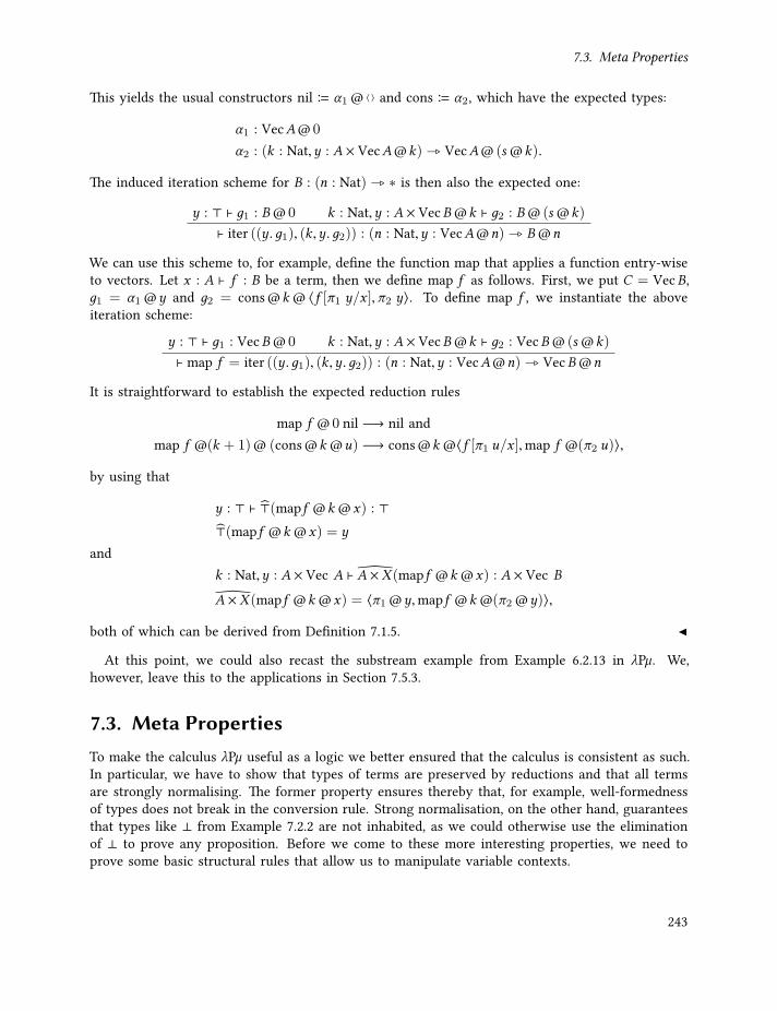
7.3. Meta Properties
This yields the usual constructors nil B α1 @ ⟨ ⟩ and cons B α2, which have the expected types:
α1 : VecA@ 0
α2 : (k : Nat,y : A × VecA@k) _ VecA@ (s @k).
The induced iteration scheme for B : (n : Nat) _ ∗ is then also the expected one:
y : ⊤ ⊢ д1 : B@ 0 k : Nat,y : A × VecB@k ⊢ д2 : B@ (s @k)
⊢ iter ((y.д1), (k,y.д2)) : (n : Nat,y : VecA@n) _ B@n
We can use this scheme to, for example, define the function map that applies a function entry-wiseto vectors. Let x : A ⊢ f : B be a term, then we define map f as follows. First, we put C = VecB,д1 = α1 @y and д2 = cons@k @ ⟨f [π1 y/x ],π2 y⟩. To define map f , we instantiate the aboveiteration scheme:
y : ⊤ ⊢ д1 : VecB@ 0 k : Nat,y : A × VecB@k ⊢ д2 : VecB@ (s @k)
⊢ map f = iter ((y.д1), (k,y.д2)) : (n : Nat,y : VecA@n) _ VecB@n
It is straightforward to establish the expected reduction rules
map f @ 0 nil −→ nil andmap f @(k + 1)@ (cons@k @u) −→ cons@k @⟨f [π1 u/x ],map f @(π2 u)⟩,
by using that
y : ⊤ ⊢ ⊤(mapf @k @x) : ⊤⊤(mapf @k @x) = y
andk : Nat,y : A × Vec A ⊢A × X (mapf @k @x) : A × Vec BA × X (mapf @k @x) = ⟨π1 @y,mapf @k @(π2 @y)⟩,
both of which can be derived from Definition 7.1.5.
At this point, we could also recast the substream example from Example 6.2.13 in λPµ. We,however, leave this to the applications in Section 7.5.3.
7.3. Meta PropertiesTo make the calculus λPµ useful as a logic we better ensured that the calculus is consistent as such.In particular, we have to show that types of terms are preserved by reductions and that all termsare strongly normalising. The former property ensures thereby that, for example, well-formednessof types does not break in the conversion rule. Strong normalisation, on the other hand, guaranteesthat types like ⊥ from Example 7.2.2 are not inhabited, as we could otherwise use the eliminationof ⊥ to prove any proposition. Before we come to these more interesting properties, we need toprove some basic structural rules that allow us to manipulate variable contexts.
243
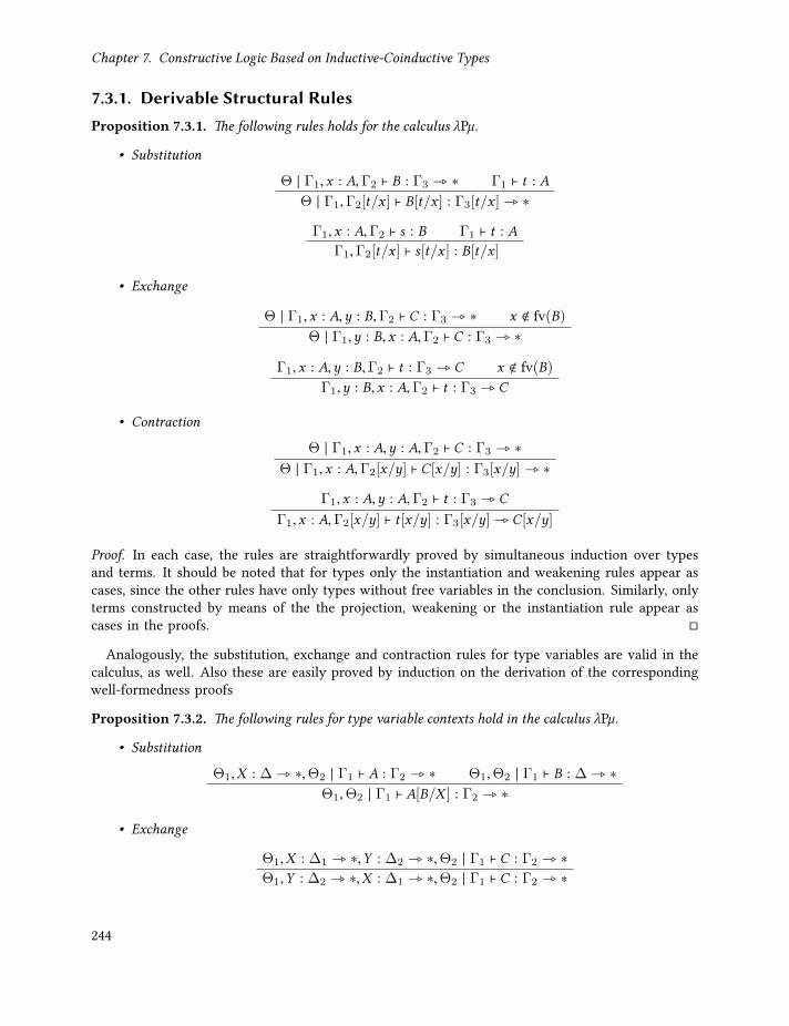
Chapter 7. Constructive Logic Based on Inductive-Coinductive Types
7.3.1. Derivable Structural RulesProposition 7.3.1. The following rules holds for the calculus λPµ.
• Substitution
Θ | Γ1,x : A,Γ2 ⊢ B : Γ3 _ ∗ Γ1 ⊢ t : AΘ | Γ1,Γ2[t/x ] ⊢ B[t/x ] : Γ3[t/x ] _ ∗Γ1,x : A,Γ2 ⊢ s : B Γ1 ⊢ t : A
Γ1,Γ2[t/x ] ⊢ s[t/x ] : B[t/x ]
• Exchange
Θ | Γ1,x : A,y : B,Γ2 ⊢ C : Γ3 _ ∗ x < fv(B)Θ | Γ1,y : B,x : A,Γ2 ⊢ C : Γ3 _ ∗
Γ1,x : A,y : B,Γ2 ⊢ t : Γ3 _ C x < fv(B)Γ1,y : B,x : A,Γ2 ⊢ t : Γ3 _ C
• Contraction
Θ | Γ1,x : A,y : A,Γ2 ⊢ C : Γ3 _ ∗Θ | Γ1,x : A,Γ2[x/y] ⊢ C[x/y] : Γ3[x/y] _ ∗
Γ1,x : A,y : A,Γ2 ⊢ t : Γ3 _ C
Γ1,x : A,Γ2[x/y] ⊢ t [x/y] : Γ3[x/y] _ C[x/y]
Proof. In each case, the rules are straightforwardly proved by simultaneous induction over typesand terms. It should be noted that for types only the instantiation and weakening rules appear ascases, since the other rules have only types without free variables in the conclusion. Similarly, onlyterms constructed by means of the the projection, weakening or the instantiation rule appear ascases in the proofs.
Analogously, the substitution, exchange and contraction rules for type variables are valid in thecalculus, as well. Also these are easily proved by induction on the derivation of the correspondingwell-formedness proofs
Proposition 7.3.2. The following rules for type variable contexts hold in the calculus λPµ.
• Substitution
Θ1,X : ∆ _ ∗,Θ2 | Γ1 ⊢ A : Γ2 _ ∗ Θ1,Θ2 | Γ1 ⊢ B : ∆ _ ∗Θ1,Θ2 | Γ1 ⊢ A[B/X ] : Γ2 _ ∗
• Exchange
Θ1,X : ∆1 _ ∗,Y : ∆2 _ ∗,Θ2 | Γ1 ⊢ C : Γ2 _ ∗Θ1,Y : ∆2 _ ∗,X : ∆1 _ ∗,Θ2 | Γ1 ⊢ C : Γ2 _ ∗
244

7.3. Meta Properties
• Contraction
Θ1,X : ∆1 _ ∗,Y : ∆2 _ ∗,Θ2 | Γ1 ⊢ C : Γ2 _ ∗Θ1,X : ∆1 _ ∗,Θ2 | Γ1 ⊢ C[X/Y ] : Γ2 _ ∗
It should be noted that the analogues of Proposition 7.3.1 and Proposition 7.3.2 are proved forpre-types and pre-terms in the Agda formalisation [Bas18b]. These are necessary there to constructthe reduction relation.
7.3.2. Subject ReductionLet us now come to a more interesting property: the preservation of types by the reduction relation.This result is stated in Theorem 7.3.4. Towards the proof of it, we need the the following key lemmafirst, which essentially states that the action of types on terms acts like a functor.
Lemma 7.3.3 (Type correctness of type action). Given the action of types on terms, see Def. 7.1.5, thefollowing inference rule holds.
X : Γ1 _ ∗ | Γ′2 ⊢ C : Γ2 _ ∗ Γ1,x : A ⊢ t : BΓ′2,Γ2,x : C(A) ⊢ C(t) : C(B)
Proof. We want to prove this lemma by induction on the derivation of X : Γ1 _ ∗ | Γ′2 ⊢ C : Γ2 _ ∗,thus we need to generalise the statement to arbitrary type constructor contexts Θ. So assumethat Θ is a context, such that Θ = X1 : Γ1 _ ∗, . . . ,Xn : Γn _ ∗, that Θ | Γ′ ⊢ C : Γ _ ∗ andΓi ,x : Ai ⊢ ti : Bi terms for i = 1, . . . ,n. Our goal is then to show that Γ′,Γ,x : C(
#—A) ⊢ C( #—
t ) : C(#—B ),
which we can do now by induction on the derivation of Θ | Γ′ ⊢ C : Γ _ ∗.The induction base has two cases. First, it is clear that if Θ = ∅, then #—
A = ε and C(#—A ) = C , thus
the definition is thus well-typed. Second, if C = Xi for some i , then we immediately have
C(#—A ) = C[
# —
(Γi ).A/#—X ] idΓi = ((Γi ).Ai ) idΓi −→p Ai ,
thus, by (Conv) and the type of ti , we have Γi ,x : C(#—A ) ⊢ ti : C(
#—B ) as required.
In the induction step, we have five cases for C .
• The type correctness for C in case C has been constructed by Weakening for type and termvariables is immediate by induction and the definition of F in these cases.
• C = C ′@ s and Γ = ∆[s/y] with
Θ | Γ′ ⊢ C ′ : (y : D,∆) _ ∗ Γ′ ⊢ s : DΘ | Γ′ ⊢ C ′@ s : ∆[s/y] _ ∗
By induction we have then that Γ′,y : D,∆,x : C ′(#—A ) ⊢ C ′( #—
t ) : C ′(#—A ), thus, since
C ′(#—A ) = C ′[
# —
(Γ1).A/#—X ]@idy:D,∆
= C ′[# —
(Γ1).A/#—X ]@y@id∆,
245

Chapter 7. Constructive Logic Based on Inductive-Coinductive Types
we get by Prop. 7.3.1
Γ′,∆[s/y],x : C ′[# —
(Γ1).A/#—X ]@ s @id∆[s/y]
⊢ C ′( #—t )[s/y] : C ′[
# —
(Γ1). B/#—X ]@ s @id∆[s/y].
As we now have
C ′@ s(#—A ) = (C ′@ s)[
# —
(Γ1).A/#—X ]@id∆[s/y]
= C ′[# —
(Γ1).A/#—X ]@ s @id∆[s/y]
and C ′@ s(#—t ) = C ′(
#—t )[s/y], we find that
Γ′,∆[s/y],x : C ′@ s(#—A ) ⊢ C ′@ s(
#—t ) : C ′@ s(
#—B )
as expected.
• C = (y).C ′ with Θ | Γ′,y : D ⊢ C ′ : Γ _ ∗. This gives us, by the induction hypothesis,Γ′,y : D,Γ,x : C ′(
#—A ) ⊢ C ′( #—
t ) : C ′(#—B ). Now we observe that
C ′(#—A ) = C ′[
# —
(Γ1).A/#—X ]@idΓ
←−p ((y).C ′[# —
(Γ1).A/#—X ])@y@idΓ
= C[# —
(Γ1).A/#—X ]@idy:D,Γ
= C(#—A ),
which gives us, by (Conv), that Γ′,y : D,Γ,x : C(#—A ) ⊢ C ′( #—
t ) : C(#—B ). Thus the definition(x).C ′( #—
t ) = C ′(#—t ) is well-typed.
• C = µ(Y : Γ _ ∗ ; #—σ ;#—D ) with
Θ,Y : Γ _ ∗ | ∆k ⊢ Dk : ∗ σk : ∆k ▷ Γ
Θ | ∅ ⊢ µ(Y : Γ _ ∗ ; #—σ ;#—D ) : Γ _ ∗
For brevity, we define R #—B = µ(Y : Γ _ ∗ ; #—σ ;
#—D [
#—B /
#—X ]). Then, by induction, we have
Γ,x : Dk (#—A ,R #—
B ) ⊢ Dk (#—t ,x) : Dk (
#—B ,R #—
B )
Now we have that Dk (#—A ,R #—
B ) = Dk [# —
(Γi ).A/#—X ][R #—
B /Y ]. Note that the second substitutiondoes not contain a parameter abstraction, as R #—
B is closed. If we define
дk = αk @id∆k @(Dk
( #—t , idR #—B
) ),
246

7.3. Meta Properties
where αk refers to α µ(Y :Γ_∗ ; #—σ ;#—D [
# —
(Γi ). B/#—X ])
k (see the definition of F ), then we can derive thefollowing.
⊢ αk : ∆k (Dk (#—A ,R #—
B ) _ R #—B @σk ) (Inst)
∆k ⊢ αk @id∆k : Dk (#—A ,R #—
B ) _ R #—B @σk (Inst)
∆k ,x : Dk [# —
(Γi ).A/#—X ][R #—
B /Y ] ⊢ дk : R #—B (Ind-E)
Γ ⊢ iter# —
(∆k ,y′.дk )@idΓ : R #—
A @idΓ _ R #—B @idΓ (Inst)
Γ,x : R #—A @idΓ ⊢ iter
# —
(∆k ,y′.дk )@idΓ @x : R #—
B @idΓFinally, we have
C(#—A ) = µ(Y : Γ _ ∗ ; #—σ ;
#—D )[
# —
(Γi ).A/#—X ]@idΓ = R #—
A @idΓ,
which implies, by the above derivitations, that we indeed have
Γ,x : C(#—A ) ⊢ C( #—
t ) : C(#—B ).
• C = ν(Y : Γ _ ∗ ; #—σ ;#—D ). This case is treated analogously to that for inductive types.
This concludes the induction, thus (7.3.3) indeed holds for types C with one free variable.
The following is now an easy consequence of Lemma 7.3.3.
Theorem 7.3.4 (Subject reduction). If Γ ⊢ t1 : A and t1 −→ t2, then Γ ⊢ t2 : A.
Proof. Lemma 7.3.3 gives us immediately subject reduction for the contraction relation. Since thereduction relation is the compatible closure of contraction, type preservation −→ follows at once.
7.3.3. Strong NormalisationThis section is devoted to show that all well-formed terms of λPµ are strongly normalising, whichmeans that all reduction sequences in the calculus terminate. We would intuitively expect this, giventhat we introduced the reduction relation by following the homomorphism property of (co)recursionfor initial and final dialgebras. But since the proof is not obvious, we fully present it here.
The proof of strong normalisation uses the saturated sets approach, see for example [Geu94]. Inthis approach, one defines a model of strongly normalising (pre-)terms for the types as follows. First,we define what it means for a set of pre-terms to be saturated, where, most importantly, all termsin a saturated set are strongly normalising. Next, we give an interpretation JAK of dependent typesA as families of saturated sets. Finally, we show that if Γ ⊢ t : A, then for all assignments ρ ofterms to variables in Γ, we have t ∈ JAK(ρ). This proof proceeds by induction on the derivation ofΓ ⊢ t : A, and the interpretation of terms as saturated sets give us precisely the necessary inductionhypothesis for this proof to go through. Since JAK(ρ) ⊆ SN, strong normalisation for all well-formedterms follows.
Towards this model, we need to define all of the above concepts, starting with a few basic notations.
Definition 7.3.5. We use the following notations.
247

Chapter 7. Constructive Logic Based on Inductive-Coinductive Types
• Λ is the set of pre-terms.
• SN is the set of strongly normalising pre-terms.
• ⌈Γ⌉ is the set of variables in context Γ.
For simplicity, we identify context morphisms σ : Γ1 ▷ Γ2 and valuations ρ : ⌈Γ2⌉ → Λ, if weknow that the terms of ρ are typeable in Γ1. This allows us to write σ(x) for x ∈ ⌈Γ2⌉, and M @ ρfor pre-terms M . It is helpful though to make explicit the action of context morphisms on valuations,essentially given by composition, and write
Jσ : Γ1 ▷ Γ2K : Λ ⌈Γ1 ⌉ → Λ ⌈Γ2 ⌉Jσ : Γ1 ▷ Γ2K(γ )(y) = σ(y)[γ ].(7.3)
Saturated sets are defined by containing certain open terms (base terms) and by being closed underkey reductions. The idea of base terms is that they are neutral, i.e. they do not admit any reductions,but it is possible to substitute variables so that new reductions are possible. Moreover, they willensure that all variables are in the interpretation of types as saturated sets, see Definition 7.3.8.Key redexes, on the other hand, will allow us to prove that saturated sets are backwards closedunder constructors for inductive types and coiteration for coinductive types, see Lemma 7.3.22 andLemma 7.3.24. We introduce these two notions in the following two definitions.
Definition 7.3.6 (Base Terms). The set of base terms B is defined inductively by the following threeclosure rules.
• Var ⊆ B
• iter# —
(Γk ,x .Nk )@σ @M ∈ B, provided that M ∈ B, Nk ∈ SN and σ ∈ SN.
• ξν (X :Γ_∗ ; #—τ ;
#—A )
k @σ @M ∈ B, provided that M ∈ B, σ ∈ SN and ∃γ . (σ = Jτk K(γ )).
Definition 7.3.7 (Key Redex). A pre-term M is a redex, if there is a P with M ≻ P . M is the keyredex
1. of M itself, if M is a redex,
2. of iter# —
(Γk ,yk .Nk )@σ @N , if M the key redex of N , or
3. of ξk @σ @N , if M the key redex of N .
We denote by redk (M) the term that is obtained by contracting the key redex of M .
Note that a key redex is given both for inductive and coinductive types by the correspondingelimination principles (iteration and destructors, respectively).
We are now in the position to define what a saturated set is.
Definition 7.3.8 (Saturated Sets). A set X ⊆ Λ is saturated, if
1. X ⊆ SN
248

7.3. Meta Properties
2. B ⊆ X
3. If redk (M) ∈ X and M ∈ SN, then M ∈ X .
We denote by SAT the set of all saturated sets.
It is easy to see that SN ∈ SAT, and that every saturated set is non-empty. Moreover, it is easyto show that SAT is a complete lattice with set inclusion as order. Besides these standard facts, wewill use the following constructions on saturated sets.
Definition 7.3.9. Let Γ be a context. We define a semantical context extension (comprehension) ofpairs (E,U ) with E ⊆ Λ ⌈Γ⌉ and U : E → SAT with respect to a given variable x < ⌈Γ⌉ by
(E,U )x =ρ[x 7→ M]
ρ ∈ E and M ∈ U (ρ), (7.4)
where ρ[x 7→ M] : ⌈Γ⌉ ∪ x → Λ extends ρ by mapping x to M . Moreover, we define a semanticalversion of the typing judgement:
E ⊩ U = M | ∀γ ∈ E. M[γ ] ∈ U (γ ). (7.5)
We now show that we can give a model of well-formed types by means of saturated sets. Toachieve this, we define simultaneously an interpretation of contexts and the interpretation of types.The intention is that we have that
• if ⊢ Γ Ctx, then JΓK is the set of valuations for variables in Γ with JΓK ⊆ Λ ⌈Γ⌉ ;
• if ⊢ Θ TyCtx, then JΘK(X ) : JΓK→ SAT for all X : Γ _ ∗ in Θ, and
• if Θ | Γ1 ⊢ A : Γ2 _ ∗, then JAK : JΘK × JΓ1,Γ2K→ SAT.
Definition 7.3.10 (Interpretations). We interpret type variable contexts, term variable contexts andtypes simultaneously. First, we assign to each term context is a set of allowed possible valuations:
J∅K B ! : ∅ → ΛJΓ,x : AK B (JΓK, JAK)x = ρ[x 7→ M] | ρ ∈ JΓK and M ∈ JAK(ρ)For Θ = X1 : Γ1 _ ∗, . . . ,Xn : Γn _ ∗ we define
JΘK B ∏Xi ∈ ⌈Θ⌉
IΓi ,
where IΓ is the set of valuations that respect convertibility:
IΓ = U : JΓK→ SAT | ∀ρ, ρ ′. ρ −→T ρ ′⇒ U (ρ) = U (ρ ′)
Finally, we define in Fig. 7.6 the interpretation of types as families of term sets. In the clause forinductive types, A∆
k denotes the type that is obtained by weakening Γk ⊢ Ak : ∗ to ∆,Γk ⊢ A∆k : ∗,
π : (Γk ,y : A∆k ) ▷ Γk projects y away, and Jσk • πK∗(U ) B U Jσk • πK is the reindexing for set
families.
249

Chapter 7. Constructive Logic Based on Inductive-Coinductive Types
J⊢ ⊤ : ∗K(δ , ρ) = ∩X ∈ SAT | ⟨ ⟩ ∈ X JΘ,X : Γ _ ∗ | ∅ ⊢ X : Γ _ ∗K(δ , ρ) = δ(X )(ρ)JΘ,X | Γ1 ⊢ A : Γ2 _ ∗K(δ , ρ) = JΘ | Γ1 ⊢ A : Γ2 _ ∗K(δ | ⌈Θ⌉ , ρ)JΘ | Γ1,x : B ⊢ A : Γ2 _ ∗K(δ , ρ) = JΘ | Γ1 ⊢ A : Γ2 _ ∗K(δ , ρ | ⌈Γ1 ⌉)JΘ | Γ1 ⊢ A@ t : Γ2[t/x ] _ ∗K(δ , ρ) = JΘ | Γ1 ⊢ A : (x : B,Γ2) _ ∗K(δ , ρ[x 7→ t [ρ]])JΘ | Γ1 ⊢ (x).A : (x : B,Γ2) _ ∗K(δ , ρ) = JΘ | Γ1,x : B ⊢ A : Γ2 _ ∗K(δ , ρ)JΘ | ∅ ⊢ µ(X : Γ _ ∗ ; #—σ ;
#—A ) : Γ _ ∗K(δ , ρ) =
M | ∀U ∈ IΓ. ∀∆. ∀k . ∀Nk ∈JΓk K,JA∆
k K(δ [X 7→ U ])y ⊩ Jσk • πK∗(U ).
iter# —
(Γk ,y.Nk )@ ρ@M ∈ U (ρ)
JΘ | ∅ ⊢ ν(X : Γ _ ∗ ; #—σ ;#—A ) : Γ _ ∗K(δ , ρ) =
M | ∃U ∈ IΓ. ∀k . ∀γ ∈ Jσk K−1(ρ). ξk @γ @M ∈ JAk K(δ [X 7→ U ],γ )
Figure 7.6.: Interpretation of types as families of saturated sets
Most of the clauses in the interpretation in Figure 7.6 are straightforward. The only two interestingcases are the recursive types. In both the inductive and the coinductive case we interpret the typesas sets that are closed under the corresponding elimination principles. For inductive case we usethereby a least fixed point, impredicatively defined by the use of a universal quantification. Onthe other hand, coinductive types are interpreted as a greatest fixed point by means of existentialquantification.
Before we continue stating the key results about this interpretation of types, let us briefly lookat an example.
Example 7.3.11. Suppose A,B are closed types. Recall that the function space was defined byA → B = ν(X : ∗ ; ε1 : (x : A) ▷ ∅;B), and the application by t a = ξ1 @a@ t . Note that theconditition γ ∈ Jε1K−1(ρ) reduces to γ (x) ∈ JAK because Jε1K(γ )(y ∈ ∅) = ρ(y)[ε1] holds for anyγ ∈ J(x : A)K. So we write N instead of γ (x). We further note that, since A, B and thus A→ B areclosed, we can leave out the type variable valuation δ . Taking all of this into account, we obtain
JA→ BK(γ ) = M | ∀N ∈ JAK. ξ1 @γ @M ∈ JBK= M | ∀N ∈ JAK.M N ∈ JBK,
which is the usual definition definition, see [Geu94].
We just state here the key lemmas and the main result.65 The interested reader may find the proofsand the supporting lemmas in Section 7.3.4 below.
Lemma 7.3.12 (Soundness of type action). Suppose C is a type with Θ | Γ ⊢ C : Γ′ _ ∗ that Θ isa type variable context with Θ = X1 : Γ1 _ ∗, . . . ,Xn : Γn _ ∗. Assume further that that for allparameters ∆ ⊢ r : C ′ occurring in C and τ : ∆′ ▷ ∆, we have r [τ ] ∈ JC ′K(τ ). Let δA,δB ∈ JΘK andΓi ,x : Ai ⊢ ti : Bi , such that for all σ ∈ JΓiK, ti ∈ δB(Xi )(τ ). Then for all contexts ∆, all σ : ∆ ▷ Γ,Γ′
250

7.3. Meta Properties
and all s ∈ JCK(δA,σ)C(
#—t )[σ , s] ∈ JCK(δB ,σ). (7.6)
Lemma 7.3.13. The interpretation of types J−K given in Def. 7.3.10 is well-defined and JAK(δ , ρ) ∈ SATfor all A,δ , ρ.
Lemma 7.3.14 (Soundness). If Γ ⊢ t : A, then for all ρ ∈ JΓK we have t [ρ] ∈ JAK(ρ).From the soundness, we immediately derive strong normalisation.
Theorem 7.3.15. All well-typed terms are strongly normalising, that is, if Γ1 ⊢ t : Γ2 _ A then t ∈ SN.
Proof. We first note that terms only reduce if Γ2 = ∅. In that case we can apply we can applyLem. 7.3.14 with ρ being the identity, so that t ∈ JAK(ρ). Thus, by Lem. 7.3.13 and the definition ofsaturated sets, we can conclude that t ∈ SN. Since t does not reduce if Γ2 is non-trivial, we alsohave in that case that t ∈ SN. Hence every well-typed term is strongly normalising.
7.3.4. Soundness proof for saturated sets modelIn this section, we present the technical details of the proof of the soundness Lemma 7.3.14 and theresults leading up to it. These details are presented here mainly for completeness and without muchfurther comment, as it is not expected that the reader will dive into the details at first read.
This first lemma proves that the composition of context morphisms is the same as the compositionof their interpretation.
Lemma 7.3.16. For all σ : Γ1 ▷ Γ2 and τ : Γ2 ▷ Γ3 we have Jτ • σK = Jτ K JσK.Proof. For all ρ : ⌈Γ1⌉ → Λ and x ∈ ⌈Γ3⌉ we have
Jτ • σK(ρ)(x) = (τ • σ)(x)[ρ] = τ (x)[σ ][ρ]
= Jτ K(JσK(ρ))(x) = (Jτ K JσK)(ρ)(x)as required.
Next, we show that instantiation of types is given equivalently by updating valuations.
Lemma 7.3.17. If Γ1 ⊢ A : Γ2 _ ∗, σ : Γ1 ▷ Γ2 and ρ ∈ JΓ1K, then JA@σK(ρ) = JAK([ρ, JσK(ρ)]),where [ρ, JσK(ρ)] ∈ JΓ1,Γ2K is given by
[ρ, JσK(ρ)] (x) = ρ(x), x ∈ ⌈Γ1⌉JσK(ρ)(x), x ∈ ⌈Γ2⌉
.
Proof. Simply by repeatedly applying the case of the semantics of type instantiations.
The following four lemmas 7.3.18-7.3.21 are easily proved by induction on the derivation of well-formedness of the corresponding type A.
Lemma 7.3.18. If Γ1,x : B,Γ2 ⊢ A : ∗ and Γ1 ⊢ t : B, then for all ρ ∈ JΓ1,Γ2[t/x ]K we haveJA[t/x ]K = JAK(ρ[x 7→ t ]).
251
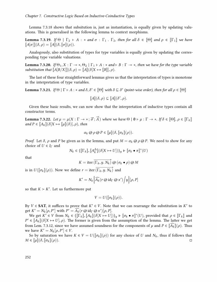
Chapter 7. Constructive Logic Based on Inductive-Coinductive Types
Lemma 7.3.18 shows that subsitution is, just as instantiation, is equally given by updating valu-ations. This is generalised in the following lemma to context morphisms.
Lemma 7.3.19. If Θ | Γ2 ⊢ A : ∗ and σ : Γ1 ▷ Γ2, then for all δ ∈ JΘK and ρ ∈ JΓ1K we haveJA[σ ]K(δ , ρ) = JAK(δ , JσK(ρ)).Analogously, also substitution of types for type variables is equally given by updating the corres-
ponding type variable valuations.
Lemma 7.3.20. If Θ1,X : Γ _ ∗,Θ2 | Γ1 ⊢ A : ∗ and ⊢ B : Γ _ ∗, then we have for the type variablesubstitution that JA[B/X ]K(δ , ρ) = JAK(δ [X 7→ JBK], ρ).
The last of these four straightforward lemmas gives us that the interpretation of types is monotonein the interpretation of type variables.
Lemma 7.3.21. If Θ | Γ ⊢ A : ∗ and δ ,δ ′ ∈ JΘK with δ ⊑ δ ′ (point-wise order), then for all ρ ∈ JΘKJAK(δ , ρ) ⊆ JAK(δ ′, ρ).
Given these basic results, we can now show that the interpretation of inductive types contain allconstructor terms.
Lemma 7.3.22. Let µ = µ(X : Γ _ ∗ ; #—σ ;#—A ) where we have Θ | ∅ ⊢ µ : Γ _ ∗. If δ ∈ JΘK, ρ ∈ JΓk K
and P ∈ JAk K(δ [X 7→ JµK(δ)], ρ), thenαk @ ρ@ P ∈ JµK(δ , Jσk K(ρ)).
Proof. Let δ , ρ and P be given as in the lemma, and put M = αk @ ρ@ P . We need to show for anychoice of U ∈ IΓ and
Nk ∈ JΓk K, JA∆k K(δ [X 7→ U ])y ⊩ Jσk • πK∗(U )
thatK = iter
# —
(Γk ,y.Nk )@ (σk • ρ)@M
is in U (Jσk K(ρ)). Now we define r = iter# —
(Γk ,y.Nk ) and
K ′ = Nk
[Ak (r @idΓ @x ′)
/y][ρ, P ]
so that K ≻ K ′. Let us furthermore put
V = U (Jσk K(ρ)).By V ∈ SAT, it suffices to prove that K ′ ∈ V . Note that we can rearrange the substitution in K ′ toget K ′ = Nk [ρ, P
′] with P ′ = Ak (r @idΓ @x ′)[ρ, P ].We get K ′ ∈ V from Nk ∈ JΓk K, JAk K(δ [X 7→ U ])y ⊩ Jσk • πK∗(U ), provided that ρ ∈ JΓk K and
P ′ ∈ JAk K(δ [X 7→ U ], ρ). The former is given from the assumption of the lemma. The latter we getfrom Lem. 7.3.12, since we have assumed soundness for the components of µ and P ∈ JAk K(ρ). Thuswe have K ′ = Nk [ρ, P
′] ∈ V .So by saturation we have K ∈ V = U (Jσk K(ρ)) for any choice of U and Nk , thus if follows that
M ∈ JµK(δ , Jσk K(ρ)).
252
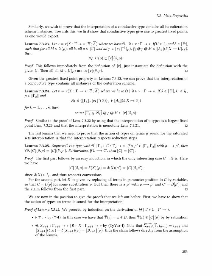
7.3. Meta Properties
Similarly, we wish to prove that the interpretation of a coinductive type contains all its coiterationscheme instances. Towards this, we first show that coinductive types give rise to greatest fixed points,as one would expect.
Lemma 7.3.23. Let ν = ν(X : Γ _ ∗ ; #—σ ;#—A ) where we have Θ | ∅ ⊢ ν : Γ _ ∗. IfU ∈ IΓ and δ ∈ JΘK,
such that for all M ∈ U (ρ), all k , all ρ ∈ JΓK and all γ ∈ Jσk K−1(ρ), ξk @γ @M ∈ JAk K(δ [X 7→ U ],γ ),then
∀ρ.U (ρ) ⊆ JνK(δ , ρ).Proof. This follows immediately from the definition of JνK, just instantiate the definition with thegiven U . Then all all M ∈ U (ρ) are in JνK(δ , ρ).
Given the greatest fixed point property in Lemma 7.3.23, we can prove that the interpretation ofa coinductive type contains all instances of the coiteration scheme.
Lemma 7.3.24. Let ν = ν(X : Γ _ ∗ ; #—σ ;#—A ) where we have Θ | ∅ ⊢ ν : Γ _ ∗. If δ ∈ JΘK, U ∈ IΓ,
ρ ∈ JΓk K andNk ∈ JΓk K, Jσk K∗(U )y ⊩ JAk K(δ [X 7→ U ])
for k = 1, . . . ,n, thencoiter
# —
(Γk ,y.Nk )@ ρ@M ∈ JνK(δ , ρ).Proof. Similar to the proof of Lem. 7.3.22 by using that the interpretation of ν-types is a largest fixedpoint Lem. 7.3.23 and that the interpretation is monotone Lem. 7.3.21.
The last lemma that we need to prove that the action of types on terms is sound for the saturatedsets interpretation is that the interpretation respects reduction steps.
Lemma 7.3.25. Suppose C is a type with Θ | Γ1 ⊢ C : Γ2 _ ∗. If ρ, ρ ′ ∈ JΓ1,Γ2K with ρ −→ ρ ′, then∀δ . JCK(δ , ρ) = JCK(δ , ρ ′). Furthermore, if C −→ C ′, then JCK = JC ′K.Proof. The first part follows by an easy induction, in which the only interesting case C = X is. Herewe have JCK(δ , ρ) = δ(X )(ρ) = δ(X )(ρ ′) = JCK(δ , ρ ′),since δ(X ) ∈ IΓi and thus respects conversions.
For the second part, let D be given by replacing all terms in parameter position in C by variables,so that C = D[ρ] for some substitution ρ. But then there is a ρ ′ with ρ −→ ρ ′ and C ′ = D[ρ ′], andthe claim follows from the first part.
We are now in the position to give the proofs that we left out before. First, we have to show thatthe action of types on terms is sound for the interpretation.
Proof of Lemma 7.3.12. We proceed by induction on the derivation of Θ | Γ ⊢ C : Γ′ _ ∗.• ⊢ ⊤ : ∗ by (⊤-I). In this case we have that ⊤(ε) = x ∈ B, thus ⊤(ε) ∈ JCK(δ) by by saturation.
• Θ,Xn+1 : Γn+1 _ ∗ | ∅ ⊢ X : Γn+1 _ ∗ by (TyVar-I). Note that Xn+1(#—t , tn+1) = tn+1 andJXn+1K(δ ,σ) = δ(Xn+1)(σ) = JBn+1K(σ). thus the claim follows directly from the assumption
of the lemma.
253

Chapter 7. Constructive Logic Based on Inductive-Coinductive Types
• Θ,X : Γ′′ _ ∗ | Γ ⊢ C : Γ′ _ ∗ by (TyVar-Weak). Immediate by induction.
• Θ | Γ,y : D ⊢ C : Γ′ _ ∗ by (Ty-Weak). Again immediate by induction.
• Θ | Γ ⊢ C @ r : Γ′[s/x ] _ ∗ with Γ ⊢ r : C ′ by (Ty-Inst). First, we note that σ = (σ1,σ2)with σ1 : ∆ ▷ Γ and σ2 : ∆ ▷ Γ′[σ1, r ]. Let us put τ = (σ1, r [σ1],σ2), so that we have(C @ r)(
#—t )[σ , s] = C(
#—t )[s/x ][σ , s] = C(
#—t )[σ1, r [σ1],σ2, s] = C(
#—t )[τ , s].
By the assumption of the lemma on parameters we have r [σ1] ∈ JC ′K(σ1), and thus τ ∈JΓ,x : C ′[σ1],Γ′[σ1, r [σ1]]K, which gives JC @ rK(δ ,σ) = JCK(δ ,τ ). By induction, we haveC(
#—t )[τ , s] ∈ JCK(δ ,τ ), and it follows that(C @ r)(
#—t )[σ , s] ∈ JC @ rK(δ ,σ).
• Θ | Γ1 ⊢ (x). B : (x : A,Γ2) _ ∗ by (Param-Abstr). Immediate by induction.
• Θ | ∅ ⊢ µ(Y : Γ _ ∗ ; #—τ ;#—D ) : Γ _ ∗ by (FP-Ty). We abbreviate, as before, this type just by
µ. Recall the definition of µ:
µ(#—t ) = iterRA
# —
(∆k ,x .дk )@idΓ @x
with дk = αk @id∆k @(Dk
( #—t ,y
) )and RA = µ[
# —
(Γi ).Ai /#—X ]
for Θ,Y : Γ _ ∗ | ∆k ⊢ Dk : ∗
Now, put δ ′ = δ [Y 7→ JRBK], then we have by induction that Dk (#—t ,y)[id∆k ,y] ∈ JDk K(δ ′, id∆k ).
Since idΓk ∈ SNwe have by Lem. 7.3.22 for all ρ ∈ J∆k , Dk (#—A,RB)K that дk [ρ] ∈ JµK(δ , Jτk K(ρ)).
By assumption, we have s ∈ JRAK(σ), hence by choosing U = JRBK in the definition of JRAKwe find µ(
#—t )[σ , s] ∈ JRBK(σ) = JµK(δ ,σ).
• Θ | ∅ ⊢ ν(Y : Γ _ ∗ ; #—τ ;#—D ) : Γ _ ∗ by (FP-Ty). Analogous to the case for inductive types,
only that we use Lemma 7.3.24.
Finally, we can use all of the above results to show that the interpretation of types as saturatedsets is sound with respect to the typing rules of λPµ.
Proof of Lemma 7.3.14. We proceed by induction on the type derivation for t . Since t does not haveany parameters, we only have to deal with fully applied terms and will thus leave out the case forinstantiation in the induction. Instead, we will have cases for fully instantiated α , ξ , etc. So letρ ∈ JΓK and proceed by the cases for t .
• ⟨ ⟩ ∈ J⊤K(ρ) by definition.
• For Γ,x : A ⊢ x : A we have x [ρ] = ρ(x). From the definition of JΓ,x : AK, we obtainρ(x) ∈ JΓ ⊢ A : ∗K(ρ | ⌈Γ⌉) = JΓ,x : A ⊢ A : ∗ K(ρ). Thus x [ρ] ∈ JAK(ρ) as required.
• Weakening is dealt with immediately by induction.
254

7.4. Dependent Iteration
• If t is of type B by (Conv), then by induction t ∈ JAK(ρ). Since by Lem. 7.3.25 JBK(ρ) = JAK(ρ),we have t ∈ JBK(ρ).
• Suppose we are given µ = µ(X : Γ _ ∗ ; #—σ ;#—A ) and ∆ ⊢ αk @τ @ t : µ[σk • τ ] with τ : ∆ ▷ Γ
and ∆ ⊢ t : Ak [µ/X ][τ ].Then, by induction, we have t ∈ JAk K(X 7→ JµK,τ ) and soundness for the components of µ,thus by Lem. 7.3.22
αk @τ @ t ∈ JµK(Jσk • τ K(ρ)) = Jµ[σk • τ ]K(ρ).• Suppose we have µ = µ(X : Γ _ ∗ ; #—σ ;
#—A ) and ∆ ⊢ iterµ # —
(Γk ,x .дk )@τ @ t : C @τ . Then byinduction we get from ∆ ⊢ t : µ[τ ] that t ∈ Jµ[τ ]K(ρ), hence if we chose U = JC @τ K andNk = дk the definition of JµK yields iterµ
# —
(Γk ,x .дk )@τ @ t ∈ JC @τ K(ρ).• Suppose we have ν = ν(X : Γ _ ∗ ; #—σ ;
#—A ), and ∆ ⊢ ξk @τ @ t : Ak [ν/X ][τ ] with τ : ∆ ▷ Γk
and with ∆ ⊢ t : ν [σk • τ ]. By induction, t ∈ Jν [σk • τ ]K(ρ) thus there is a U such thatξk @τ @ t ∈ JAk K(X 7→ U , Jτ K(ρ)). By Lem. 7.3.23 and Lem. 7.3.21 we thus obtain thatξk @τ @ t ∈ JAk K(X 7→ JνK, Jτ K(ρ)). Since JAk K(X 7→ JνK, Jτ K(ρ)) = JAk [ν/X ][τ ]K(ρ), theclaim follows.
• For coiter-terms we just apply Lem. 7.3.24, similar to the αk -case.
This concludes the induction, thus the interpretation of types is sound with respect to the typingjudgement for terms.
7.4. Dependent IterationIn Section 7.1 we have introduced the calculus λPµ of dependent inductive and coinductive types.As we saw in Section 7.2, this calculus subsumes all of first-order intuitionistic logic or Martin-Löftype theory. However, we were not able to define the second projection for dependent coproductsor existential quantifiers. Similarly, we are also not able to carry out proofs by induction in λPµ.Both of these problems are rectified once we extend the calculus with a dependent iteration scheme,cf. Section 6.4.2.
The goal of the present section is to propose an extension of λPµ by a dependent iteration principlefor inductive types. Such a dependent iteration principle will be necessary to carry out the proofsin the application section below. For now it is left open whether the calculus that results fromextending λPµ with dependent iteration is still strongly normalising. It seems, however, that theproof we gave in Section 7.3.3 can be adapted accordingly.
One may ask what the dual extension of λPµ for coinductive types is that corresponds to dependentiteration. It is clear that there is no such thing as dependent coiteration that generalises coiterationin the way dependent iteration extends iteration. As we discussed in Section 6.4.3 the dual conceptof induction is the bisimulation proof principle, which we referred to as coinduction. We will notextend λPµ here with coinduction, rather we will discuss possible future work in this direction inSection 7.6.
255

Chapter 7. Constructive Logic Based on Inductive-Coinductive Types
(⊢ ⊤ : ∗)(θ) = ⊤(Θ,X : Γ _ ∗ | ∅ ⊢ X : Γ _ ∗)(θ ,B) = YX @idΓ,y:B@idΓ
(Θ,X | Γ1 ⊢ A : Γ2 _ ∗)(θ ,B) = A(θ)
(Θ | Γ1,x : B ⊢ A : Γ2 _ ∗)(θ) = A(θ)
(Θ | Γ1 ⊢ A@ t : Γ2[t/x ] _ ∗)(θ) = A[t/x ]
(Θ | Γ1 ⊢ (x).A : (x : B,Γ2) _ ∗)(θ) = A(θ)(Θ | ∅ ⊢ ρ(X : Γ _ ∗ ; #—σ ;
#—A ) : Γ _ ∗)(θ) = ρ(X : Γ, z : R@id _ ∗ ; #—σ ′;
#—A ′)@idΓ,y
where R = ρ(Y : Γ _ ∗ ; #—σ ;#—A )
σ ′k = (σ ,αk @id@yk )
A′k = Ak (θ ,R)[θ ]
Figure 7.7.: Lifting of Dependent Types to Predicates
To be able to formulate the dependent iteration scheme, we first need to lift types to predicates.As in Section 6.4.1, a predicate is here meant to be a type that depends on terms of the type thatit is a predicate for. More precisely, given a type B with ⊢ B : ∆ _ ∗, a B-predicate is a type Pwith Γ,x : B@id∆ ⊢ P : ∗. A lifting of an open type A with X : ∆ _ ∗ | Γ ⊢ A : ∗ to B-predicatesis then a type A(B) with a free type variable that ranges over B-predicates, cf. Definition 2.5.7. Inother words, the lifting should satisfy the following rule.
X : ∆ _ ∗ | Γ ⊢ A : ∗ ⊢ B : ∆ _ ∗Y : (∆,x : B@id∆) _ ∗ | Γ,y : A[B/X ] ⊢ A(B) : ∗
We give such a lifting in the following definition. That the above rule holds is proved below.
Definition 7.4.1. Let A be a type with Θ | Γ1 ⊢ A : Γ2 _ ∗ and θ be a sequence of types, suchthat θ = B1 : ∆1 _ ∗, . . . ,Bn : ∆n _ ∗ if Θ = X1 : ∆1 _ ∗, . . . ,Xn : ∆n _ ∗. We define thenthe lifting A(θ) of A to predicates over θ . If Θ is empty, we just put A() = ⊤. Otherwise, A is byinduction on the well-formedness derivation of A in Figure 7.6.
The following lemma shows that the predicate lifting results in well-formed types. This will enableus to prove subject reduction.
Lemma 7.4.2. The following rule holds for the predicate lifting in Definition 7.4.1.
X : ∆ _ ∗ | Γ ⊢ A : ∗ ⊢ B : ∆ _ ∗Y : (∆,x : B@id∆) _ ∗ | Γ,y : A[B/X ] ⊢ A : ∗
Proof. Let us write, analogously to the notation for context morphisms, θ : Θ1 ▷Θ2, if θ is a sequenceof types in context Θ1 that matches Θ2. More precisely, θ is a sequence constructed by the followingtwo rules.
() : Θ1 ▷ ∅θ : Θ1 ▷Θ2 ⊢ B : Γ _ ∗(θ ,B) : Θ1 ▷ (Θ2,X : Γ _ ∗)
256

7.4. Dependent Iteration
Given such a sequence θ : ∅ ▷Θ of types, we define a lifted context Θ(θ) as follows by induction.
∅(θ) = ∅(Θ,X : Γ _ ∗)(θ ,B : Γ _ ∗) = Θ(θ),Y : (Γ,B@idΓ) _ ∗
This allows us to give a typing rule for the general lifting that we can use in a proof by induction.
Θ | Γ1 ⊢ A : Γ2 _ ∗ θ : ∅ ▷ΘΘ(θ) | Γ1,Γ2,y : A[θ ]@idΓ2
⊢ A : ∗(7.7)
If we can show that this typing rule holds, then we are done because the typing rule of the lemmaholds then by picking Θ = X : ∆ _ ∗, Γ1 = Γ and Γ2 = ∅. The rule (7.7) can now be shownby a straightforward induction on the typing derivation of A. Details are provided in the Agdaformalisation [Bas18b].
Definition 7.4.3. We define an extension of λPµ with a dependent iteration principle as follows.66Suppose that µ(X : Γ _ ∗ ; #—
f ;#—A ) is an inductive type, which we refer to as µ here. Dependent
iteration is a term diter# —
(Γk ,yk , zk .дk ) that is subject to the following typing rule.
∆ ⊢ C : (Γ,x : µ@idΓ) _ ∗∆,Γk ,yk : Ak [µ/X ], zk : Ak (µ)[C/X ] ⊢ дk : (C @σk @ (αk @idΓk @yk )) ∀1 ≤ k ≤
#—A
(D-Rec)
∆ ⊢ diter # —
(Γk ,yk , zk .дk ) : (Γ,y : µ@idΓ) _ C @idΓ @y
Additionally, we introduce an induction principle for the type ⊤. This induction principle is givenby terms diter⊤ д, subject to the following rule.
Γ ⊢ C : (x : ⊤) _ ∗ Γ ⊢ д : C @ ⟨ ⟩(D-Rec-⊤)
Γ ⊢ diter⊤ д : (y : ⊤) _ C @y
We refer to the extension of λPµ by the above dependent iteration and induction principles byλPµ+. The contraction relation of λPµ+ on terms is given by that of λPµ with the additional followingtwo clauses: one for general dependent iteration
diter# —
(Γk ,yk , zk .дk )@(σk • τ )@(αk @τ @u)
≻ дk[Ak (diter
# —
(Γk ,yk .дk )@idΓ @x)/zk
][τ ,u]
and one for the induction principle for ⊤
diter⊤ д ⟨ ⟩ ≻ д.
The reduction relation of λPµ+ is then again the compatible closure of its contraction relation.
Let us illustrate the usefulness of the extended calculus λPµ+ by means of two examples.
257

Chapter 7. Constructive Logic Based on Inductive-Coinductive Types
Example 7.4.4. Let us first derive that ⟨ ⟩ is the unique inhabitant of ⊤, which allows us to generallyignore variables of type ⊤. We write
s A t B EqA(s, t)
and if A is understood from the context, we drop the subscript. The proposition we thus want toprove is
y : ⊤ ⊢ y ⟨ ⟩ : ∗,
in other words, we need to establish a term canon⊤ with
y : ⊤ ⊢ canon⊤ : y ⟨ ⟩.
This term is given by canon⊤ B diter⊤ refl@y, as we show now. First, we put
C B (y).y ⟨ ⟩
and thus have C @y ≡ y ⟨ ⟩. Since refl : ⟨ ⟩ ⟨ ⟩, we then obtain
⊢ C : (y : ⊤) _ ∗ ⊢ refl : C @ ⟨ ⟩(D-Rec-⊤)⊢ diter⊤ refl : (y : ⊤) _ C @y
(Inst)y : ⊤ ⊢ diter⊤ refl@y : C @y
(Conv)y : ⊤ ⊢ canon⊤ : y ⟨ ⟩
This proves that ⟨ ⟩ is the unique inhabitant of ⊤, up to propositional equality. Our main use of thisfact is to eliminate variables of type ⊤, that is, we consider terms t with Γ,x : ⊤ ⊢ t : A to beessentially the same as terms s with Γ ⊢ s : A.
The following example shows that we can now define a second projection for coproduct types,we thereby show that coproducts are strong in λPµ+, cf. Definition 6.3.2 and Section 6.4.2.
Example 7.4.5. In Example 7.2.6 we have seen that the existential quantifier can be represented by
∃x : A. B = µ(X : ∗ ; ε1;B),
where ε1 : (x : A) ▷ ∅ is the empty context morphism. Moreover, we have also seen there that thefirst projection π1 : (∃x : A. B)→ A can be defined by simple iteration. The goal of this example isto show that dependent iteration allows us to define also the second projection
π2 : Π(z : ∃x : A. B). B[π1 z/x ].
In other words, under the assumption of dependent iteration, the existential quantifier is becomesa strong sum67 or coproduct type, cf. Section 6.4.2.
First, we note that, since B has no free type variable, the predicate lifting B is defined to be thetype ⊤. Thus, the dependent iteration scheme for the existential quantifier amounts to the followingrule.
Γ ⊢ C : (∃x : A. B) _ ∗ Γ,x : A,y : B ⊢ д : C @⟨x ,y⟩(D-Rec-∃)
Γ ⊢ diter (x ,y.д) : (z : (∃x : A. B)) _ C @ z
258
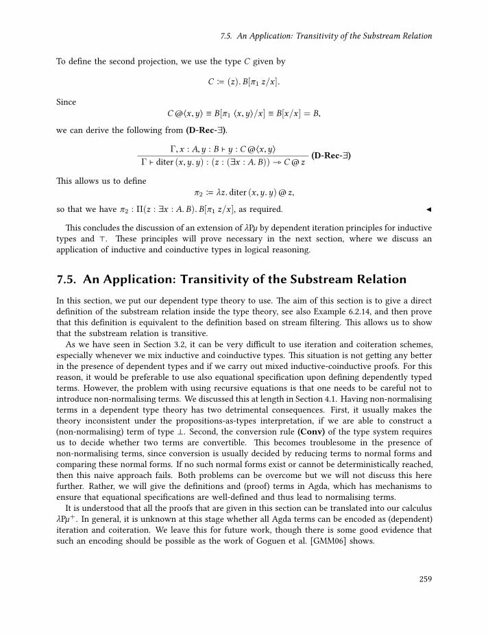
7.5. An Application: Transitivity of the Substream Relation
To define the second projection, we use the type C given by
C B (z). B[π1 z/x ].
SinceC @⟨x ,y⟩ ≡ B[π1 ⟨x ,y⟩/x ] ≡ B[x/x ] = B,
we can derive the following from (D-Rec-∃).Γ,x : A,y : B ⊢ y : C @⟨x ,y⟩
(D-Rec-∃)Γ ⊢ diter (x ,y.y) : (z : (∃x : A. B)) _ C @ z
This allows us to defineπ2 B λz. diter (x ,y.y)@ z,
so that we have π2 : Π(z : ∃x : A. B). B[π1 z/x ], as required.
This concludes the discussion of an extension of λPµ by dependent iteration principles for inductivetypes and ⊤. These principles will prove necessary in the next section, where we discuss anapplication of inductive and coinductive types in logical reasoning.
7.5. An Application: Transitivity of the Substream RelationIn this section, we put our dependent type theory to use. The aim of this section is to give a directdefinition of the substream relation inside the type theory, see also Example 6.2.14, and then provethat this definition is equivalent to the definition based on stream filtering. This allows us to showthat the substream relation is transitive.
As we have seen in Section 3.2, it can be very difficult to use iteration and coiteration schemes,especially whenever we mix inductive and coinductive types. This situation is not getting any betterin the presence of dependent types and if we carry out mixed inductive-coinductive proofs. For thisreason, it would be preferable to use also equational specification upon defining dependently typedterms. However, the problem with using recursive equations is that one needs to be careful not tointroduce non-normalising terms. We discussed this at length in Section 4.1. Having non-normalisingterms in a dependent type theory has two detrimental consequences. First, it usually makes thetheory inconsistent under the propositions-as-types interpretation, if we are able to construct a(non-normalising) term of type ⊥. Second, the conversion rule (Conv) of the type system requiresus to decide whether two terms are convertible. This becomes troublesome in the presence ofnon-normalising terms, since conversion is usually decided by reducing terms to normal forms andcomparing these normal forms. If no such normal forms exist or cannot be deterministically reached,then this naive approach fails. Both problems can be overcome but we will not discuss this herefurther. Rather, we will give the definitions and (proof) terms in Agda, which has mechanisms toensure that equational specifications are well-defined and thus lead to normalising terms.
It is understood that all the proofs that are given in this section can be translated into our calculusλPµ+. In general, it is unknown at this stage whether all Agda terms can be encoded as (dependent)iteration and coiteration. We leave this for future work, though there is some good evidence thatsuch an encoding should be possible as the work of Goguen et al. [GMM06] shows.
259
Chapter 7. Constructive Logic Based on Inductive-Coinductive Types
7.5.1. Some Preliminaries in Agda
This first section is devoted to the introduction of the propositions-as-types interpretation in Agdasyntax. We will interleave the given Agda code with the necessary explanation. All the indentedcode is formally verified in Agda and will be explained as we go.
We start off by introducing the propositions-as-types interpretation in its own module calledPropsAsTypes. Agda allows the separation of code into modules that can be imported in other files,as we will see later.
module PropsAsTypes where
Inside the module, we now introduce our first type, which implements the dependent sum thatwe encountered earlier. The following code declares a new inductive data type called Σ with twoparameters I and X . So far, we denoted the universe of valid types by ∗, whereas Agda uses thenotation Set instead. Thus, I is a type parameter. The parameter X , on the other hand, is a familyof types. In our syntax, we would denote this by X : (i : I) _ ∗ and instantiation of X with aparameter t would be written as X @ t . Agda uses for types with parameters the same notation asfor the function space,68 so that the instantiation of X is written as X t .
Another mechanism of Agda that appears in the definition of Σ is that I is an implicit parameter,signified by the curly braces, and that X is an explicit parameter. The idea of the implicit parametermechanism is that Agda ought to be able to infer the argument I from the context. For example, ifwe have a type U : Nat → Set, then Agda can infer from the instantiation ΣU that I needs to beinstantiated with Nat. Should this inference not be possible, then one can always resort to writingΣ NatU to explicitly give the parameter I . We will see this below in the definition of the binaryproduct.
The type Σ itself has one constructor “,” with two arguments, where the argument positions aremarked by the underscores. This allows us to write (i,x) if i : I and x : X i , thereby resembling thepairing notation that we used before.
data Σ I : Set (X : I → Set) : Set where_, _ : (i : I) → X i → Σ X
In Example 7.2.6, we denoted the type Σ by ∃ to emphasise its relation to existential quantification.This was done in the light of the fact that the iteration scheme for that type corresponded exactly tothe usual elimination rule the existential quantifier. Later we introduced dependent iteration, whichwe could use in Example 7.4.5 to define both projections from the existential type. In this section, wewill distinguish between Σ as a data type, which has both projections, and the existential quantifieras a proposition. The latter will only come with the non-dependent elimination principle.
We now give the dependent iteration scheme for the dependent sum type Σ. Let A be a typefamily that depends on Σ X , that is, A : Σ X → Set. Recall from Example 7.4.5 that, if we want toeliminate ΣX into A, then we need to provide a term of type A (i,x) with parameters i : I and x : X i .Such a term can equivalently be given as a dependent function f of type Πi : I .Πx : X i .A (i,x).In Agda, this function type is written as (i : I) → (x : X i) → A (i , x), in the style of de Bruijn’stelescopes [dBru68]. Conveniently, we can define the dependent iteration scheme in Agda then byusing pattern matching as follows.
260

7.5. An Application: Transitivity of the Substream Relation
drec−Σ : I : Set X : I → Set A : Σ X → Set →((i : I) → (x : X i) → A (i , x)) →(u : Σ X) → A u
drec−Σ f (i , x) = f i x
It is also straightforward to define, as we did in Example 7.4.5, the two projections for thedependent sum by appealing to dependent iteration.
π₁ : I : Set X : I → Set → Σ X → Iπ₁ = drec−Σ (λ i x → i)
π₂ : I : Set X : I → Set → (u : Σ X) → X (π₁ u)π₂ = drec−Σ (λ i x → x)
From the dependent sum type we can also derive the binary product type. Note that we introducedthis type before as a coinductive type. It saves us here, however, some work to define the binaryproduct in terms of the dependent sum.
_×_ : Set → Set → SetA × B = Σ A λ _ → B
In the propositions-as-types interpretation, one uses a type system to represent logical propositions.To make clear whenever we write a proof of a proposition that has been internalised into Agda, wewill use Prop instead of Set. Thus, if ϕ is a proposition that we encoded in Agda, we will denotethis as ϕ : Prop. This notation is introduced by the following definition.
Prop = Set
An important logical connective that we will need later is conjunction. Even though conjunctionis defined in terms the binary product, we use separate notations to emphasise its logical nature.
_∧_ : Prop → Prop → PropA ∧ B = A × B
∧−elim₁ : A₁ A₂ : Prop → A₁ ∧ A₂ → A₁∧−elim₁ = π₁
∧−elim₂ : A₁ A₂ : Prop → A₁ ∧ A₂ → A₂∧−elim₂ = π₂
∧−intro : A₁ A₂ : Prop → A₁ → A₂ → A₁ ∧ A₂∧−intro a₁ a₂ = (a₁ , a₂)
As already mentioned, we also introduce a separate notation for the existential quantifier.
∃ : X : Set → (A : X → Prop) → Prop∃ = Σ
261
Chapter 7. Constructive Logic Based on Inductive-Coinductive Types
Agda allows us to provide a syntax for the existential quantifier that matches the usual notationwith explicit quantification domain. It is not so relevant to precisely understand the followingdefinition, the reader should just remember that we can write ∃[ x ∈ X ] A instead of ∃x : X .A forpropositions A with a free occurrence of x .
∃−syntax : ∀ X → (X → Prop) → Prop∃−syntax X A = ∃ A
syntax ∃−syntax X (λ x → A) = ∃[ x ∈ X ] A
From the pairing constructor and the iteration scheme for the dependent sum type we obtain theusual introduction and elimination rules for the existential quantifier that we already discussed inExample 7.2.6. For convenience, we also provide a scheme for the simultaneous elimination of twoexistential quantifiers. None of these definitions should come at a surprise to the reader at this stage.
∃−intro : X : Set A : X → Prop → (x : X) → A x → ∃[ x ∈ X ] (A x)∃−intro x a = (x , a)
∃−elim : X : Set A : X → Prop B : Prop →((x : X) → A x → B) → ∃[ x ∈ X ] (A x) → B
∃−elim = drec−Σ
∃₂−elim : X Y : Set A : X → Prop B : Y → Prop C : Prop →((x : X) (y : Y) → A x → B y → C) →∃[ x ∈ X ] (A x) → ∃[ x ∈ Y ] (B x) → C
∃₂−elim f p q = ∃−elim (λ x p′ → ∃−elim (λ y q′ → f x y p′ q′) q) p
Finally, we define bi-implication between propositions, which is is of course just given as theconjunction of implications in both directions.
_⇔_ : Prop → Prop → PropA ⇔ B = (A → B) ∧ (B → A)
equivalence : A B : Prop → (A → B) → (B → A) → A ⇔ Bequivalence = ∧−intro
Having set up the necessary definitions of the propositions-as-types interpretation, we can nowmove to more interesting topics.
7.5.2. Streams and BisimilarityTo define the substream relation, we first need to introduce streams. We have done this already inthe simple type system in Example 3.1.2 but to have a complete example, we recast the definition ofstreams here again in Agda. This allows us to also explain the syntax of Agda’s coinductive types.Moreover, we will introduce bisimilarity on streams as a coinductively defined relation and provethat it is an equivalence relation.
262
7.5. An Application: Transitivity of the Substream Relation
module Stream where
Before we come to the actual definitions, we import a few modules that we use throughout thissection. The module Relation.Binary contains definitions surrounding binary relations. In particular,we can write R : Rel A to express that R is a type with two parameters of type A, that is, if R isof type A → A → Set. We will later show that bisimilarity of streams implies point-wise equality.Since point-wise equality is defined in terms of indexing into streams by natural numbers, we alsoneed to import the module Data.Nat. Finally, the module PropsAsTypes was given in Section 7.5.1above.
import Relation.Binary as BinRel
open import Data.Nat using (ℕ; zero; suc)open import PropsAsTypes
Let us now come to the definition of streams and their corresponding coiteration principle. Thefollowing coinductive record type corresponds to what we have called so far codata types. Thus,instead of
codata Stream (A : Set) : Set wherehd : Atl : Stream A
the type of streams is given in Agda by the following record type.
record Stream (A : Set) : Set wherecoinductivefieldhd : Atl : Stream A
A record type in Agda is a type that is defined by its destructors, which are called fields inAgda. If a record is recursive, that is, it uses itself in its own definition, then we need to specifywhether it this recursion is to be interpreted inductively or coinductively. Since we never encounterinductive record types here, we stick to the codata terminology. The reader should thus just replacethe verbose coinductive record syntax in her head by the simpler codata syntax.
The coiteration principle for streams is given in Agda by the following equational specification.
coiter : X A : Set → (X → A × X) → (X → Stream A)coiter c x .hd = π₁ (c x)coiter c x .tl = coiter c (π₂ (c x))
Note that we define the coiteration principle in terms of copattern equations, which are the sameas in the calculus λµν=. Agda ensures that this definition is well-formed by performing coveringand guardedness checks.69 These checks intuitively work for coinductive types as follows. First, ifwe specify an element of a coinductive type, like for example a stream, then we are required tospecify the outcome of each destructor. In the case of streams, we need to give both head and tail
263

Chapter 7. Constructive Logic Based on Inductive-Coinductive Types
of a stream. Second, the guardedness condition requires that the element we are specifying doesnot occur in another term on the right-hand side of an equation. This ensures that the result of adestructor application does not depend on this very result itself, an instance of which we have seenin Example 4.1.18. Note that coiter, as given above, is thus well-defined because it appears directlyand in another term on the right-hand side of the equation that specifies the tail.
It is possible, though very tedious, to translate all the following equational specification intoinstances of iteration and coiteration schemes. But this translation largely obscures the proof ideaand so we refrain from carrying it out. However, we should also make clear that this translationfrom such Agda specifications into the given calculus has the status of a conjecture for the timebeing. Some evidence that such a translation should be possible is given by [Gim95] and [GMM06].
The following two functions are straightforward definitions of higher derivatives of streams, thatis, repeated applications of the tail destructor, and indexing of stream positions by natural numbers.Since we have seen such definitions before, we will not explain these further here.
δ : ∀A → ℕ → Stream A → Stream Aδ 0 s = sδ (suc n) s = δ n (s .tl)
_at_ : ∀A → Stream A → ℕ → As at n = (δ n s) .hd
We now come to the definition of bisimilarity for streams. In Example 6.2.13, we defined streambisimilarity as a coinductive relation in the category theoretical setup of recursive type closedcategories. The idea of that definition was that stream bisimilarity is given by two destructors: onethat extracts from a proof of bisimilarity a proof that the heads of related streams are equivalent,and one that extracts a bisimilarity proof for their tails. To facilitate reuse, we define bisimilarityin terms of a so called setoid, which is a set A together with an equivalence relation ≈ on it. Sucha pair is given by the term S of type Setoid. To avoid further complications, we directly introducenames for the carrier A of the setoid, the relation ≈ and for the proof that that ≈ is an equivalencerelation.
module Bisim (S : Setoid) whereopen BinRel.Setoid Srenaming (Carrier to A; _≈_ to _≈_; isEquivalence to S-equiv)
Given such a setoid, let us now define bisimilarity for streams over A. We define it as a binaryrelations that can be written in infix notation. This is signalled by the following declaration, whichsays that ∼ is a relation with two positions (marked by the underscores). The relation itself is thendefined as a coinductive type in the expected way.
record _~_ (s t : Stream A) : Prop wherecoinductivefieldhd≈ : s .hd ≈ t .hdtl~ : s .tl ~ t .tl
264
7.5. An Application: Transitivity of the Substream Relation
Since bisimilarity is a coinductive type, it comes with a coiteration principle. This principle is,as we have explained in Example 6.2.13, by the usual bisimulation proof (or coinduction) principle.We briefly show how this principle can be derived from equational specifications. First, we definewhat it means for a relation R to be a bisimulation on streams. This is witnessed by the followingpredicate on relations, which should be intuitively clear: A relation R is a bisimulation if for allstreams s and t that are related by R, their heads must be equivalent (in the setoid A) and their tailsmust again be related by R.
isBisim : Rel (Stream A) → PropisBisim _R_ = ∀ s t → s R t → (s .hd ≈ t .hd) ∧ (s .tl R t .tl)
Given this notion of bisimulation relation we can now derive the usual proof principle:
∃−bisim→~ : ∀ _R_ → isBisim _R_ →∀ (s t : Stream A) → s R t → s ~ t
∃−bisim→~ R−isBisim s t q .hd≈ = ∧−elim₁ (R−isBisim s t q)∃−bisim→~ R−isBisim s t q .tl~ =
∃−bisim→~ R−isBisim (s .tl) (t .tl) (∧−elim₂ (R−isBisim s t q))
Note the striking similarity to the coiteration principle for streams, only that in this case we constructa bisimilarity proof rather than a stream. Let us briefly go through the types that appear in thedefinition of ∃−bisim→ . First, we are given a binary relation R and the following arguments.
R−isBisim : isBisim R
s, t : Stream A
q : s R t
To show that s and t are bisimilar, we need to provide now proofs that their heads are equivalentand that the tails are related. These are the two copattern cases of ∃−bisim→ . By the definition ofisBisim, we have
R−isBisim s t : (s .hd ≈ t .hd) ∧ (s .tl R t .tl).
Thus, the first conjunction elimination gives us the sought after proof for the head case. The tailcase is given by recursively constructing a bisimilarity proof for the tails from the second part ofthe above conjunction. This should intuitively clarify how proofs of coinductive predicates are givenin Agda, and it should also highlight the similarity to the definition of the coiteration principle forstreams.
As a sanity check for the correctness of the definition of bisimilarity, we prove that bisimilarstreams are point-wise equivalent.
bisim→ext−≈ : ∀ s t → s ~ t → (∀ n → s at n ≈ t at n)bisim→ext−≈ p zero = p .hd≈bisim→ext−≈ p (suc n) = bisim→ext−≈ (p .tl~) n
We finish this section by showing that bisimilarity is an equivalence relation, where we appealto the fact that ≈ is an equivalence relation. This allows us to show that streams form a setoid with
265
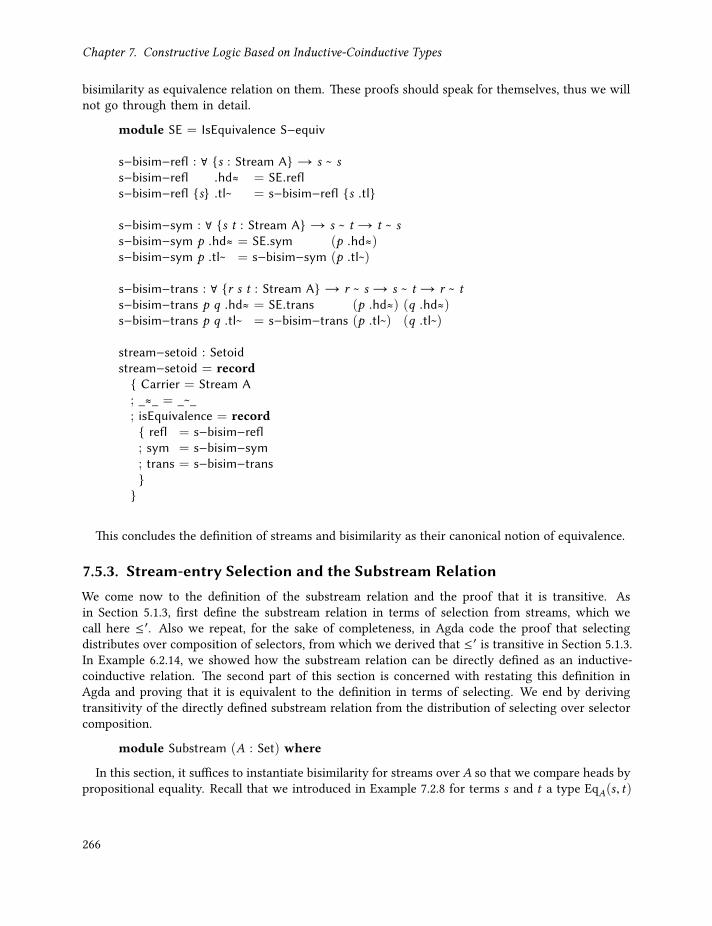
Chapter 7. Constructive Logic Based on Inductive-Coinductive Types
bisimilarity as equivalence relation on them. These proofs should speak for themselves, thus we willnot go through them in detail.
module SE = IsEquivalence S−equiv
s−bisim−refl : ∀ s : Stream A → s ~ ss−bisim−refl .hd≈ = SE.refls−bisim−refl s .tl~ = s−bisim−refl s .tl
s−bisim−sym : ∀ s t : Stream A → s ~ t → t ~ ss−bisim−sym p .hd≈ = SE.sym (p .hd≈)s−bisim−sym p .tl~ = s−bisim−sym (p .tl~)
s−bisim−trans : ∀ r s t : Stream A → r ~ s → s ~ t → r ~ ts−bisim−trans p q .hd≈ = SE.trans (p .hd≈) (q .hd≈)s−bisim−trans p q .tl~ = s−bisim−trans (p .tl~) (q .tl~)
stream−setoid : Setoidstream−setoid = record Carrier = Stream A; _≈_ = _~_; isEquivalence = record refl = s−bisim−refl; sym = s−bisim−sym; trans = s−bisim−trans
This concludes the definition of streams and bisimilarity as their canonical notion of equivalence.
7.5.3. Stream-entry Selection and the Substream RelationWe come now to the definition of the substream relation and the proof that it is transitive. Asin Section 5.1.3, first define the substream relation in terms of selection from streams, which wecall here ≤′. Also we repeat, for the sake of completeness, in Agda code the proof that selectingdistributes over composition of selectors, from which we derived that ≤′ is transitive in Section 5.1.3.In Example 6.2.14, we showed how the substream relation can be directly defined as an inductive-coinductive relation. The second part of this section is concerned with restating this definition inAgda and proving that it is equivalent to the definition in terms of selecting. We end by derivingtransitivity of the directly defined substream relation from the distribution of selecting over selectorcomposition.
module Substream (A : Set) where
In this section, it suffices to instantiate bisimilarity for streams over A so that we compare heads bypropositional equality. Recall that we introduced in Example 7.2.8 for terms s and t a type EqA(s, t)
266

7.5. An Application: Transitivity of the Substream Relation
with one constructor: refl : (x : A) _ EqA(x ,x). This types is meant to model propositional equality,that it, the notion of equality on A internal to the type theory. In Agda, propositional equality is abinary relation _≡_, which we import from the module Relation.Binary. Since propositional equalityis an equivalence relation, (A,≡) is a setoid. Thus, we can instantiate Bisim that setoid to obtainthat streams over A form a setoid with bisimilarity.
open import Relation.Binaryopen import Relation.Binary.PropositionalEquality renaming (setoid to ≡−setoid)open import PropsAsTypesopen import Stream
open Bisim (≡−setoid A)
Recall that we defined in Example 3.2.11 the type of stream selectors Sel to be the inductive-coinductive type νX . µY .X + Y , and that the first unfolding Selµ to the finitary steps was given byµY . Sel + Y . In Agda, we declare these types mutually as follows, where we directly give readablenames to the corresponding destructors and constructors.
mutualrecord Sel : Set wherecoinductivefield out : Selμ
data Selμ : Set wherepres : Sel → Selμdrop : Selμ → Selμ
Given this definition of selectors, we can define selection from streams exactly as in Example 3.2.11by the following equational specification.
selectμ : Selμ → Stream A → Stream Aselect : Sel → Stream A → Stream A
select x = selectμ (x .out)
selectμ (pres x) s .hd = s .hdselectμ (pres x) s .tl = select x (s .tl)selectμ (drop u) s = selectμ u (s .tl)
Stream selecting allows us now to define the first version of the substream relation.70 Since it willturn out to be useful to be explicit about the x selector that witnesses that s is a substream of t ,we first define a ternary relation. This relation should be read as saying that if s ≤μ[x] t, then s is asubstream of t witnessed by the selector x . In the later proofs, we also need to be able to witnessthe substream relation by elements of Selµ , hence we also introduce the corresponding version ofthe substream relation.
267
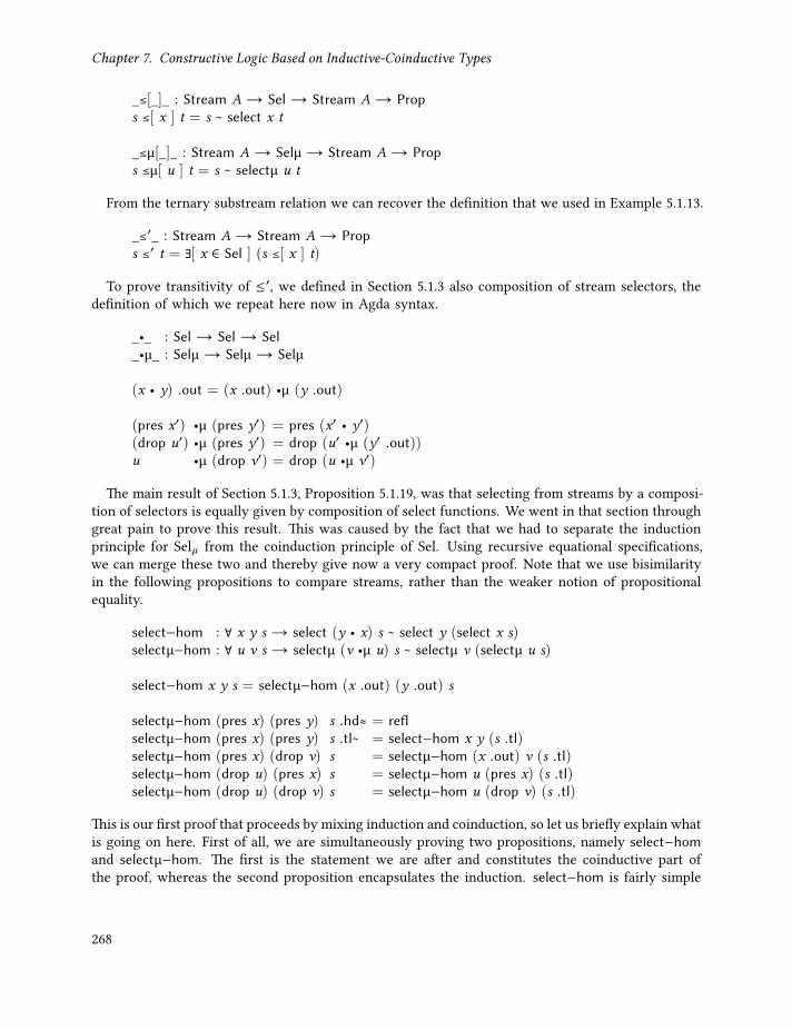
Chapter 7. Constructive Logic Based on Inductive-Coinductive Types
_≤[_]_ : Stream A → Sel → Stream A → Props ≤[ x ] t = s ~ select x t
_≤μ[_]_ : Stream A → Selμ → Stream A → Props ≤μ[ u ] t = s ~ selectμ u t
From the ternary substream relation we can recover the definition that we used in Example 5.1.13.
_≤′_ : Stream A → Stream A → Props ≤′ t = ∃[ x ∈ Sel ] (s ≤[ x ] t)
To prove transitivity of ≤′, we defined in Section 5.1.3 also composition of stream selectors, thedefinition of which we repeat here now in Agda syntax.
_•_ : Sel → Sel → Sel_•μ_ : Selμ → Selμ → Selμ
(x • y) .out = (x .out) •μ (y .out)
(pres x′) •μ (pres y′) = pres (x′ • y′)(drop u′) •μ (pres y′) = drop (u′ •μ (y′ .out))u •μ (drop v′) = drop (u •μ v′)
The main result of Section 5.1.3, Proposition 5.1.19, was that selecting from streams by a composi-tion of selectors is equally given by composition of select functions. We went in that section throughgreat pain to prove this result. This was caused by the fact that we had to separate the inductionprinciple for Selµ from the coinduction principle of Sel. Using recursive equational specifications,we can merge these two and thereby give now a very compact proof. Note that we use bisimilarityin the following propositions to compare streams, rather than the weaker notion of propositionalequality.
select−hom : ∀ x y s → select (y • x) s ~ select y (select x s)selectμ−hom : ∀ u v s → selectμ (v •μ u) s ~ selectμ v (selectμ u s)
select−hom x y s = selectμ−hom (x .out) (y .out) s
selectμ−hom (pres x) (pres y) s .hd≈ = reflselectμ−hom (pres x) (pres y) s .tl~ = select−hom x y (s .tl)selectμ−hom (pres x) (drop v) s = selectμ−hom (x .out) v (s .tl)selectμ−hom (drop u) (pres x) s = selectμ−hom u (pres x) (s .tl)selectμ−hom (drop u) (drop v) s = selectμ−hom u (drop v) (s .tl)
This is our first proof that proceeds by mixing induction and coinduction, so let us briefly explain whatis going on here. First of all, we are simultaneously proving two propositions, namely select−homand selectμ−hom. The first is the statement we are after and constitutes the coinductive part ofthe proof, whereas the second proposition encapsulates the induction. select−hom is fairly simple
268

7.5. An Application: Transitivity of the Substream Relation
and is only used in the case when we have to prove that the tails of of both outputs are bisimilar(second case of selectμ−hom). In the proof of the second proposition selectμ−hom, we proceed byinduction on the two Selµ arguments. The cases that appear here are essentially those that appearin the definition of selector composition. Note, however, that in the last two cases of selectμ−homwe do the same. At the time of writing, they both need to be there for Agda to be able to reducethe definition of •μ while checking the correctness of the proof. This is a slight nuisance, whichmight be improved in the future though.
To use that selecting preserves composition for proving transitivity of ≤′, we will need thefollowing lemma. This lemma states that selecting respects bisimilarity, that is, bisimilar streams aremapped to bisimilar streams by select.
select−resp~ : ∀s t (x : Sel) → s ~ t → select x s ~ select x tselectμ−resp~ : ∀s t (u : Selμ) → s ~ t → selectμ u s ~ selectμ u t
select−resp~ x p = selectμ−resp~ (x .out) p
selectμ−resp~ (pres x) p .hd≈ = p .hd≈selectμ−resp~ (pres x) p .tl~ = select−resp~ x (p .tl~)selectμ−resp~ (drop u) p = selectμ−resp~ u (p .tl~)
We are now in the position to show that the relation ≤′ is transitive. To do so, we first showtransitivity for the substream relation with explicit witnesses. This proof proceeds by chainingtogether bisimilarity proofs that are given in the begin … block. Since the technicalities of howsuch blocks can be defined in Agda would lead us of track, we will skip these details and just explainthe intuition of the proof. By definition of r ≤[x ] s , p is a proof of r ∼ select (x •y) t . Inside the block,we write this as r ∼⟨p⟩ select (x • y) t . Next, we use that selecting respects bisimilarity to replaces by select y t . Finally, we turn the composition of selecting into composition of the witnessingselectors. This proves r ∼ select (x • y) t , which is by definition r ≤[x • y] t . The proof term≤−select−trans could be given by using transitivity of bisimilarity (S.trans) twice, but the presentedversion is certainly preferable in terms of readability.
≤−select−trans : ∀r s t x y → r ≤[ x ] s → s ≤[ y ] t → r ≤[ x • y ] t≤−select−trans r s t x y p q =begin
r~⟨ p ⟩select x s
~⟨ select−resp~ x q ⟩select x (select y t)
~⟨ S.sym (select−hom y x t) ⟩select (x • y) twheremodule S = Setoid stream−setoid
Now that we have proved transitivity with explicit witnesses, transitivity of ≤′ follows by an easymanipulation of existential quantifiers:
269

Chapter 7. Constructive Logic Based on Inductive-Coinductive Types
≤′−trans : ∀r s t → r ≤′ s → s ≤′ t → r ≤′ t≤′−trans = ∃₂−elim (λ x y p q →
∃−intro (x • y) (≤−select−trans x = x y p q))
This concludes the recasting of the proof of transitivity relation based of stream selecting in Agda.We come now to the direct definition of the substream relation as mixed inductive-coinductiverelation. The intuition for this definition was explained in Example 6.2.14, we merely repeat thedefinition here in Agda syntax.
mutualrecord _≤_ (s t : Stream A) : Prop wherecoinductivefield out≤ : s ≤μ t
data _≤μ_ (s t : Stream A) : Prop wherematch : (s .hd ≡ t .hd) → (s .tl ≤ t .tl) → s ≤μ tskip : (s ≤μ t .tl) → s ≤μ t
In the remainder of the section we show that this direct definition is equivalent to the selecting-based one and derive transitivity of ≤ from there. The first step towards this is to extract from aproof of ≤ a selector witness.
witness : s t : Stream A → s ≤ t → Selwitnessμ : s t : Stream A → s ≤μ t → Selμ
witness p .out = witnessμ (p .out≤)
witnessμ (match _ t≤) = pres (witness t≤)witnessμ (skip u) = drop (witnessμ u)
We can now use the extracted witness to show that the substream relation is included in thewitness-based substream relation and hence in the select-based substream relation.
≤−implies−select≤ : ∀s t → (p : s ≤ t) → s ≤[ witness p ] t≤μ−implies−selectμ≤ : ∀s t → (p : s ≤μ t) → s ≤μ[ witnessμ p ] t
≤−implies−select≤ s t p = ≤μ−implies−selectμ≤ (p .out≤)
≤μ−implies−selectμ≤ (match h≡ t≤) .hd≈ = h≡≤μ−implies−selectμ≤ (match h≡ t≤) .tl~ = ≤−implies−select≤ t≤≤μ−implies−selectμ≤ (skip q) = ≤μ−implies−selectμ≤ q
≤−implies−≤′ : ∀s t → s ≤ t → s ≤′ t≤−implies−≤′ p = ∃−intro (witness p) (≤−implies−select≤ p)
Conversely, we can construct from a selector witness a proof for the substream relation. Thisallows us then to show that the select-based substream relation is in included in the substreamrelation.
270

7.6. Discussion
select≤−implies−≤ : ∀s t (x : Sel) → s ≤[ x ] t → s ≤ tselectμ≤⇒≤μ : ∀s t (u : Selμ) → s ≤μ[ u ] t → s ≤μ t
select≤−implies−≤ x p .out≤ = selectμ≤⇒≤μ (x .out) p
selectμ≤⇒≤μ (pres x) p = match (p .hd≈) (select≤−implies−≤ x (p .tl~))selectμ≤⇒≤μ (drop u) p = skip (selectμ≤⇒≤μ u p)
≤′−implies−≤ : ∀s t → s ≤′ t → s ≤ t≤′−implies−≤ = ∃−elim select≤−implies−≤
Putting these to results together, we obtain a proof that the two definitions for the substreamrelation are equivalent.
≤−and−≤′−equiv : ∀ s t → s ≤ t ⇔ s ≤′ t≤−and−≤′−equiv s t = equivalence ≤−implies−≤′ ≤′−implies−≤
Finally, using this equivalence, we can derive from the fact that ≤′ is transitive that also ≤ istransitive.
≤−trans : ∀r s t → r ≤ s → s ≤ t → r ≤ t≤−trans p q = ≤′−implies−≤ (≤′−trans (≤−implies−≤′ p) (≤−implies−≤′ q))
7.6. DiscussionIn this chapter we have have introduced a type theory λPµ that is solely based on inductive andcoinductive types, following the ideas of the category theoretical development in Chapter 6. Thisis in contrast to other type theories that usually have separate type constructors for, for example,the (dependent) function space or coproducts. The result is a theory with a small set of rules for itsjudgements and reduction relation. To justify the use of our type theory as logic, we also proved thatthe reduction relation preserves types and is strongly normalising on well-typed terms. Combiningthe present theory with that in [Nor07] would give us a justification for a large part Agda’s currenttype system, especially including coinductive types.
ContributionsLet us briefly sum up the contributions made in this chapter. First of all, we introduced thedependent type theory λPµ and showed how important logical operators and type formers can berepresented in this theory. We also discussed how the, somewhat worn-out, standard example ofvectors arises as a recursive (inductive) type in λPµ. Other examples, like the substream relation,were given as an application in Section 7.5. Second, we showed that computations of terms, givenin form of a reduction relation, are meaningful, in the sense that the reduction relation preservestypes (subject reduction) and that all computations are terminating (strong normalisation). Thus,under the propositions-as-types interpretation, our type theory can serve as formal framework
271

Chapter 7. Constructive Logic Based on Inductive-Coinductive Types
for intuitionistic reasoning. Finally, we have shown how the calculus λPµ can be extended withdependent iteration to a calculus λPµ+, so that an induction principle for inductive types is alsoavailable in the propositions-as-types interpretation.
Related WorkA major source of inspiration for the setup of our type theory is categorical logic. Especially,the use of fibrations, brought forward in [Jac99], helped a great deal in understanding how thework of Hagino [Hag87] can be extended to dependent types. Another source of inspiration is theview of type theories as internal language or even free models for classes of categories, see forexample [LS88]. This view is especially important in topos theory, where final coalgebras have beenused as foundation for predicative, constructive set theory [Acz88; vdBer06; vdBdM07]. In Chapter 6we saw how these ideas can be extended to general strictly positive inductive and coinductive types,which form the category theoretical analogue of the type theory λPµ.
Let us briefly discuss other type theories that the present work relates to. Especially close is thecopattern calculus introduced in [Abe+13] and Section 3.2, as there the coinductive types are alsospecified by the types of their destructors. However, said calculus does not have dependent types,and it is based on systems of equations to define terms, whereas the calculus in the present paper isbased on iteration and coiteration schemes, similar to the calculus λµν from Section 3.1. There areother calculi that use iteration and coiteration as basis for defining operations on non-dependentinductive and coinductive types, respectively, see Section 3.4 for further discussion.
To ensure strong normalisation, the copatterns have been combined with size annotations in [AP13].Due to the nature of the reduction relation in these copattern-based calculi, strong normalisationalso ensures productivity for coinductive types or, more generally, observational normalisation,cf. Section 4.1. As another way to ensure productivity, guarded recursive types were proposedand in [Biz+16a] guarded iteration was extended to dependent types. Guarded recursive types gobeyond strictly positive types, which is what we restricted ourselves to in this chapter, but also topositive and even negative types. However, it is not clear how one can include inductive types intosuch a type theory, which are, in the author’s opinion, crucial to mathematics and computer science.Finally, in [Sac13] another type theory with type-based termination conditions and a type former forstreams has been introduced. This type theory, however, lacks again dependent coinductive types.
Future WorkThere are still some open questions, regarding the present type theory, that we wish to settle inthe future. First of all, a basic property of the reduction relation that is still missing is confluence.Second, we have constructed the type theory with certain categorical structures in mind, and itis easy to interpret the types and terms in data type closed categories as we introduced them inSection 6.2. However, one has to be careful in showing the soundness of such an interpretation, inwhich two subtleties occur. First, if for types A and B we have that A←→T B, then we had betterensured that their interpretations agree, that is JAK = JBK, because of the conversion rule of λPµ.This property corresponds to using split fibrations, instead of merely cloven fibrations, in Section 6.2,cf. [Jac99, Sec. 10.3]. The second subtlety, which might be in the way of a sound interpretation,is the definition of substitution on recursive types. However, the Beck-Chevalley condition thatwe proposed in Section 6.5 is designed precisely to give us the soundness of substitution for the
272

7.6. Discussion
interpretation of types. Though it seems that these conditions suffice to give an interpretation ofλPµ, these conditions need to be carefully checked, as we have learned from previous attempts oncategory theoretical semantics for dependent type theories [Str91].
In Section 7.4, we mentioned already that the strong normalisation proof from Section 7.3.3 doesnot subsume dependent iteration. It is expected that the proof can be extended accordingly, butthis certainly needs to be checked carefully. Moreover, one has to ask what the dual principle todependent iteration is for coinductive types. The expectation would be coinduction, that is, thatinternally provable bisimilarity of terms implies their propositional equality. However, setting upa calculus in which coinduction holds is far from trivial, if we want to preserve decidability oftype checking. In particular, this is because bisimilarity on function types corresponds to point-wise equality, so that the coinduction principle would give us therefore extensional function types,cf. Section 6.4.3 and Example 7.2.4. An idea in this direction would be to combine observational typetheory [AMS07] with ideas of cubical/homotopy type theory [Coh+16; Uni13], which would resultin more complex calculi, albeit with decidable type checking. This is inspired by an idea that wascommunicated by Conor McBride in a talk at the Agda Implementors’ Meeting XXIII in Glasgow,and it was further developed by the author in talks given at the TYPES’16 meeting [BG16b] and theChocola Seminar at the ENS Lyon in September 2016. Due to the complexity of this task, we leavethe extension of λPµ or λPµ+ with coinduction open for now.
Finally, certain acceptable facts are not provable in λPµ+, since, for instance, we do not have uni-verses. Another common feature that is missing from the type theory, is predicative polymorphism,which is in fact justified and desirable from the categorical point of view. Both extensions go in thedirection of turning the calculus into a foundation for Agda. It is expected that such extensions arestraightforward but tedious to carry out.
Notes58 Noam Chomsky, “Language and Freedom”. In “On Anarchism”, Nathan Schneider (Ed.), 2014.
59 Indeed, subject reduction is broken in Coq, which is caused by the fact that coinductive types aredefined through constructors that can be pattern matched against. Consider the following example.
1 CoInductive Stream := Cons : Stream→ Stream.2 CoFixpoint c : Stream := Cons c.3 Definition foo : c = Cons c :=4 match c as t return match t with Cons t’ ⇒ t = Cons t’ end5 with Cons _⇒ eq_refl end.6 Eval compute in foo.7 Definition bar : c = Cons c := Eval compute in foo.
In Coq 8.6, line 6 outputs
= eq_refl
: c = Cons c
but the definition in the last line leads to the error
273
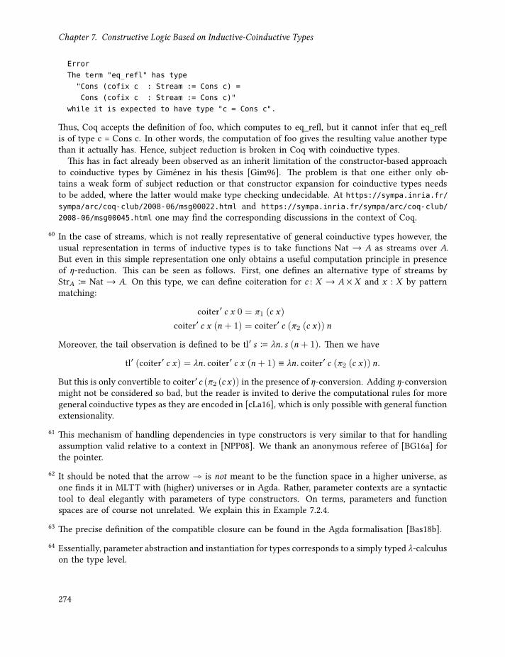
Chapter 7. Constructive Logic Based on Inductive-Coinductive Types
Error
The term "eq_refl" has type
"Cons (cofix c : Stream := Cons c) =
Cons (cofix c : Stream := Cons c)"
while it is expected to have type "c = Cons c".
Thus, Coq accepts the definition of foo, which computes to eq_refl, but it cannot infer that eq_reflis of type c = Cons c. In other words, the computation of foo gives the resulting value another typethan it actually has. Hence, subject reduction is broken in Coq with coinductive types.
This has in fact already been observed as an inherit limitation of the constructor-based approachto coinductive types by Giménez in his thesis [Gim96]. The problem is that one either only ob-tains a weak form of subject reduction or that constructor expansion for coinductive types needsto be added, where the latter would make type checking undecidable. At https://sympa.inria.fr/sympa/arc/coq-club/2008-06/msg00022.html and https://sympa.inria.fr/sympa/arc/coq-club/
2008-06/msg00045.html one may find the corresponding discussions in the context of Coq.60 In the case of streams, which is not really representative of general coinductive types however, the
usual representation in terms of inductive types is to take functions Nat → A as streams over A.But even in this simple representation one only obtains a useful computation principle in presenceof η-reduction. This can be seen as follows. First, one defines an alternative type of streams byStrA B Nat → A. On this type, we can define coiteration for c : X → A × X and x : X by patternmatching:
coiter′ c x 0 = π1 (c x)
coiter′ c x (n + 1) = coiter′ c (π2 (c x)) n
Moreover, the tail observation is defined to be tl′ s B λn. s (n + 1). Then we have
tl′ (coiter′ c x) = λn. coiter′ c x (n + 1) ≡ λn. coiter′ c (π2 (c x)) n.
But this is only convertible to coiter′c (π2 (c x)) in the presence of η-conversion. Adding η-conversionmight not be considered so bad, but the reader is invited to derive the computational rules for moregeneral coinductive types as they are encoded in [cLa16], which is only possible with general functionextensionality.
61 This mechanism of handling dependencies in type constructors is very similar to that for handlingassumption valid relative to a context in [NPP08]. We thank an anonymous referee of [BG16a] forthe pointer.
62 It should be noted that the arrow _ is not meant to be the function space in a higher universe, asone finds it in MLTT with (higher) universes or in Agda. Rather, parameter contexts are a syntactictool to deal elegantly with parameters of type constructors. On terms, parameters and functionspaces are of course not unrelated. We explain this in Example 7.2.4.
63 The precise definition of the compatible closure can be found in the Agda formalisation [Bas18b].64 Essentially, parameter abstraction and instantiation for types corresponds to a simply typed λ-calculus
on the type level.
274

7.6. Discussion
65 One interesting result, used to prove the following lemmas, is that the interpretation of types ismonotone in δ , and that the interpretation of coinductive types is the largest set closed underdestructors. This suggests that it might be possible to formulate the definition of the interpretationin categorical terms.
66 We note that the calculus with dependent iteration does not satisfy the uniqueness of identity proofs(UIP) principle. The reason is that the dependent iteration scheme amounts for EqA to
Γ,x : A,y : ⊤, z : ⊤ ⊢ д : C @x @x @(α1 @x @y)
Γ ⊢ diter (x ,y, z.д) : x : A,y : A, z : EqA(x ,y) _ C @x @y@ z
Leaving out variables of type ⊤, cf. Example 7.4.4, and writing refl s for α1 @ s @ ⟨ ⟩, we obtain fromthere the following rule.
Γ,x : A ⊢ д : C @x @x @(refl x)Γ ⊢ diter (x .д) : x : A,y : A, z : EqA(x ,y) _ C @x @y@ z
If we now try to prove that all proofs of EqA(x ,y) are given by reflexivity, we are obliged to find atype C with
C @x @x @(refl x) ≡ Eq(refl x , refl x).
A natural candidate would thus be C = (x ,y, z). Eq(z, refl x). The problem with this is that z is oftype EqA(x ,y) but refl x is of type EqA(x ,x). Hence, C is not a well-formed type.
This is of course not a formal argument that the calculus does not fulfil the UIP principle, but itgives some good evidence. For detailed discussions of the failure of UIP in Martin-Löf type theory,which should be adaptable to our calculus, see the work by Hofmann and Streicher [HS94].
67 The commonly used definition of coproducts (Σ-types) in Agda is the following.
record Σ (A : Set) (B : A → Set) : Set wherefieldproj1 : Aproj2 : B proj1
Note that the second destructor refers to the first, which is not allowed in our setup and leads to astrong elimination principle for Σ, which we obtained in Example 7.4.5 from dependent iteration.
68 In fact, X : I → Set is a function in Agda, only that it is a type in the universe Set1. This is similarto the situation in category theory, where a family of sets can be given by a functor from I , seen asa discrete category, to the category of sets. Such a functor is then an object in the large category offunctors between categories.
69 Agda also supports more sophisticated termination checks by using sized types. We will not discussthese further here though.
70 Bertot [Ber05] defines a different notion of stream selection that allows one to select from streamsby productive predicates. This way of selecting from streams is essentially equivalent to our notionof selecting by positions, see.
275


CHAPTER 8
Epilogue
Everything Faustian is far away from me. […] Thousands of questions are silenced as if dissolved. There areneither doctrines nor heresies. The possibilities are endless. Only faith in them lives creatively in me.
— Paul Klee, 1916.
Towards the end of writing this thesis, in July 2017, I was invited to give a tutorial on the topicsof Chapters 6 and 7 at the Université Savoie in the magnificent area of Lac de Bourget. This tutorialwas part of a “Workshop on Coinduction in Type Theory”, organised by Tom Hirschowitz. Theworkshop was a perfect illustration of the diversity that can be found in the views on inductionand coinduction. There were people whose main interest was indeed type theory, others camefrom a category theoretical background, and still others came from logic or base their work mostlyon classical set theory. Having all these different views leads to very stimulating but also intensediscussions, in particular because everyone has seen or used inductive-coinductive objects in someform or even worked on them.
Trying to accommodate all these different views in one thesis is impossible, and even though Itried to reach as wide an audience as possible, I had to make a selection. In the end, I chose thosetopics that give a general account to inductive-coinductive objects, in the hope that the providedtheory may serve as a foundation for reasoning about such objects. Unfortunately, selecting themore abstract theory as a focus means that many of the wonderful and interesting applications ofinductive-coinductive reasoning could not be covered here. Though one has to say that the point ofMathematics is in any case not to generate examples but to construct general theories that accountfor and explain these examples.
But I’m digressing. We have seen some usages of inductive-coinductive reasoning in this thesis,like the substream relation or the correctness proof for µ-recursion. However, there are many more,some of which we discussed in the intro, and plenty of them are not explored. For instance, Kőnig’slemma and Brouwer’s fan theorem mix inductive and coinductive reasoning, but only the latter ofwhich has been studied so far from this perspective [NUB11]. Similarly, Cauchy sequences andweak bisimilarity also involve both induction and coinduction, which again is hardly ever madeexplicit. Finally, a recurring theme in this thesis is that already the very notion of function, onwhich most of Mathematics is built, is itself coinductive. A striking consequence of this is that thecoinduction principle for function spaces, namely that bisimilarity implies equality, corresponds tothe usual principle of function extensionality: two functions are equal precisely if they agree on allarguments. This is another insight that arose from the abstract treatment of inductive-coinductiveobjects, even though I was told that this is sort of “folklore”. I hope that these examples show thatit is worthwhile to study mixed inductive-coinductive reasoning and to take it seriously. So, I hopethat this thesis may inspire others to study inductive-coinductive objects, and advance the theoryprovided here beyond its, now very basic, state.
277

Chapter 8. Epilogue
The Way OnwardSo where to go from here? There are many problems that this thesis leaves open and many directionsfor future research that it suggests. Out of those that we discussed throughout the chapters, let mehighlight a few that I deem most important.
One of the observations that we made was that iteration and coiteration schemes require a lot ofwork and ingenuity to bring mixed inductive-coinductive specifications into a form to which theseschemes can be applied. For this reason, we generally preferred specifications in terms of recursiveequations. This leaves open the problem of reconciling iteration and coiteration with recursiveequations by, for instance, expressing observationally normalising terms in λµν= as terms in λµν .A similar direction is to explore how one can dualise the principle of well-founded induction tocoiteration and coinduction. Well-founded induction can be used to implement a recursive functionby establishing a well-founded relation on its arguments and showing that the recursion descendsthe relation. Since this principle allows for fairly general recursive specifications, one has to askwhether there is a similar principle to specify productive processes.
Another major obstacle to the usability of type theories as foundation for mathematical reasoningis, in my opinion, the lack of a proper coinduction principle. The trouble is that without a coinductionprinciple, one has to explicitly use hand-crafted equivalence relations (bisimilarity) everywhere. Thisis very irritating and puts an enormous load on the user of a type theory. As we sketched inSection 7.6, it should be possible to extend λPµ+ with a coinduction principle through a combinationof ideas from observational type theory and cubical type theory. Together with type theoreticaluniverses we would obtain a type theory that covers already a large part of Mathematics andComputer Science. What is missing then are only quotients and subobjects or, more generally,colimit and limit constructions. These arise by suitably extending the dependent inductive andcoinductive types of λPµ+ — to higher inductive and coinductive types, if the reader is familiar withthese concepts. If we are able to pull off these developments, then this would lead to a type theorythat should cover, except for non-constructive proofs, most of Mathematics and Computer Science.
Apart from developments in the field of type theory, there are also other aspects of inductive-coinductive reasoning that I think need to be explored further. First of all, the logic FOL that wedeveloped in Section 5.2 needs to be fleshed out for mixed inductive-coinductive proofs. Moreover,the use of the later modality to ensure correctness of recursive proofs is not limited to bisimilarity,but should work for more general coinductive, and perhaps even for inductive-coinductive, predicatesand relations. Therefore, it would in my opinion be fruitful to explore this logic further. Next, wefound that up-to techniques allowed us to carry out the soundness proof for the logic FOL moreeasily. This seems to be a general phenomenon that needs to be explored for other logics and alsofor type theories. Finally, in the light of the goal to develop type theories that feature generalcoinduction, it would be worthwhile to study also the category theoretical side of such type theories.To be more precise, I think that it would be interesting to study Universal Coalgebra, as it wascoined by Rutten, in so-called (∞, 1)-categories. Combining all these endeavours would result in aconvergence of type theory and category theory.
278

References
[Abb03] Michael Abbott. ‘Categories of Containers’. Leicester, 2003. url: http://www.cs.le.ac.uk/people/ma139/docs/thesis.pdf (visited on 19/06/2016) (cit. on pp. 164, 190,191, 194–197, 199, 217).
[AAG05] Michael Abbott, Thorsten Altenkirch and Neil Ghani. ‘Containers: Constructing StrictlyPositive Types’. In: Theoretical Computer Science. Applied Semantics: Selected TopicsApplied Semantics: Selected Topics 342.1 (2005), pp. 3–27. issn: 0304-3975. doi: 10.1016/j.tcs.2005.06.002 (cit. on pp. 9, 164, 181, 188–191, 193, 217).
[Abe04] Andreas Abel. ‘Termination Checking with Types’. In: ITA 38.4 (2004), pp. 277–319.doi: 10.1051/ita:2004015 (cit. on p. 39).
[AA99] Andreas Abel and Thorsten Altenkirch. ‘A Predicative Strong Normalisation Proof fora Lambda-Calculus with Interleaving Inductive Types’. In: TYPES’99. Vol. 1956. LNCS.Springer, 1999, pp. 21–40. doi: 10.1007/3-540-44557-9_2 (cit. on pp. 69, 101, 103).
[AMU05] Andreas Abel, Ralph Matthes and Tarmo Uustalu. ‘Iteration and Coiteration Schemesfor Higher-Order and Nested Datatypes’. In: Theor. Comput. Sci. 333 (1-2 2005), pp. 3–66.doi: 10.1016/j.tcs.2004.10.017 (cit. on p. 9).
[AP13] Andreas Abel and Brigitte Pientka. ‘Wellfounded Recursion with Copatterns: A UnifiedApproach to Termination and Productivity’. In: ICFP. 2013, pp. 185–196. doi: 10.1145/2500365.2500591 (cit. on pp. 9, 68, 77, 126, 272, 309).
[Abe+13] Andreas Abel, Brigitte Pientka, David Thibodeau and Anton Setzer. ‘Copatterns: Pro-gramming Infinite Structures by Observations’. In: Proc. of POPL. Symposium on Prin-ciples of Programming Languages. ACM, 2013, pp. 27–38. isbn: 978-1-4503-1832-7. doi:10.1145/2429069.2429075 (cit. on pp. 9, 37, 49, 63, 65, 68, 272, 309).
[Abr90] Samson Abramsky. ‘The Lazy Lambda Calculus’. In: Research Topics in Functional Pro-gramming. Addison-Wesley, 1990, pp. 65–116 (cit. on pp. 102, 105, 152, 153).
[Acz88] Peter Aczel. Non-Well-Founded Sets. Lecture Notes 14. Center for the Study of Languageand Information, Stanford University, 1988. isbn: 0-937073-22-9 (cit. on pp. 7, 272).
[Acz+03] Peter Aczel, Jiří Adámek, Stefan Milius and Jiří Velebil. ‘Infinite Trees and CompletelyIterative Theories: A Coalgebraic View’. In: Theoretical Computer Science 300 (1–3 2003),pp. 1–45. issn: 0304-3975. doi: 10.1016/S0304-3975(02)00728-4 (cit. on p. 218).
[AM89] Peter Aczel and Nax Paul Mendler. ‘A Final Coalgebra Theorem’. In: Proceedings ofCategoryTheory and Computer Science. Vol. 389. LNCS. Springer, 1989, pp. 357–365. doi:10.1007/BFb0018361 (cit. on p. 7).
[AMV11] Jiří Adámek, Stefan Milius and Jiří Velebil. ‘Semantics of Higher-Order RecursionSchemes’. In: Logical Methods in Computer Science 7.1 (2011), pp. 1–43. doi: 10.2168/LMCS-7(1:15)2011 (cit. on p. 101).
279

References
[Agd15] Programming Logic group on Agda. Agda Documentation. Version 2.4.2.5. Chalmersand Gothenburg University, 2015. url: http://wiki.portal.chalmers.se/agda/(cit. on pp. 9, 154, 167, 224).
[AU79] Alfred V. Aho and Jeffrey D. Ullman. ‘The Universality of Data Retrieval Languages’. In:Conference Record of POPL 1979. ACM Press, 1979, pp. 110–120. doi: 10.1145/567752.567763 (cit. on p. 163).
[ACS15] Benedikt Ahrens, Paolo Capriotti and Régis Spadotti. ‘Non-Wellfounded Trees in Ho-motopy Type Theory’. In: (2015). arXiv: 1504.02949 [cs, math] (cit. on p. 224).
[AMM05] Thorsten Altenkirch, Conor McBride and James McKinna. WhyDependent Types Matter.2005. url: http://citeseerx.ist.psu.edu/viewdoc/summary?doi=10.1.1.106.8190(cit. on p. 167).
[AMS07] Thorsten Altenkirch, Conor McBride and Wouter Swierstra. ‘Observational Equality,Now!’ In: Proc. of PLPV ’07. Workshop on Programming Languages Meets ProgramVerification. ACM, 2007, pp. 57–68. isbn: 978-1-59593-677-6. doi: 10.1145/1292597.1292608 (cit. on pp. 101, 155, 273).
[AM09] Thorsten Altenkirch and Peter Morris. ‘Indexed Containers’. In: LICS. IEEE ComputerSociety, 2009, pp. 277–285. doi: 10.1109/LICS.2009.33 (cit. on pp. 181, 190).
[App+07] Andrew W. Appel, Paul-André Melliès, Christopher D. Richards and Jérôme Vouillon.‘A Very Modal Model of a Modern, Major, General Type System’. In: POPL. ACM, 2007,pp. 109–122. doi: 10.1145/1190216.1190235 (cit. on pp. 126, 137, 154).
[AM13] Robert Atkey and Conor McBride. ‘Productive Coprogramming with Guarded Recur-sion’. In: ICFP. ACM, 2013, pp. 197–208. doi: 10.1145/2500365.2500597 (cit. on pp. 68,126, 130, 132, 157).
[Awo10] Steve Awodey. Category Theory. 2nd ed. Oxford Logic Guides 52. Oxford UniversityPress, 2010. isbn: 978-0-19-923718-0 (cit. on pp. 22, 25).
[Bae09] David Baelde. ‘On the ProofTheory of Regular Fixed Points’. In: Proceedings of TABLEAUX2009. Berlin, Heidelberg: Springer Berlin Heidelberg, 2009, pp. 93–107. isbn: 978-3-642-02716-1. doi: 10.1007/978-3-642-02716-1_8 (cit. on p. 126).
[Bar85] Henk Barendregt.TheLambdaCalculus, Its Syntax and Semantics. Revised edition. Vol. 103.Studies in Logic and the Foundations of Mathematics. Amsterdam; New York; Oxford:North Holland, 1985. 621 pp. isbn: 978-0-444-87508-2 (cit. on p. 89).
[Bar91] Henk Barendregt. ‘Introduction to Generalized Type Systems’. In: J. Funct. Program.1.2 (1991), pp. 125–154. doi: 10.1017/S0956796800020025 (cit. on p. 182).
[Bar13] Henk Barendregt. ‘Foundations of Mathematics from the Perspective of ComputerVerification’. In: Mathematics, Computer Science and Logic - A Never Ending Story: TheBruno Buchberger Festschrift. Springer, 2013, pp. 1–49. isbn: 978-3-319-00966-7. doi:10.1007/978-3-319-00966-7_1 (cit. on p. 9).
[BDS13] Henk Barendregt, Wil Dekkers and Richard Statman. Lambda Calculus with Types.Cambridge ; New York: Cambridge University Press, 2013. 854 pp. isbn: 978-0-521-76614-2 (cit. on pp. 39, 68, 69, 105, 168).
280

[Bar93] Michael Barr. ‘Terminal Coalgebras in Well-Founded Set Theory’. In: Theoretical Com-puter Science 114.2 (1993), pp. 299–315. doi: 10.1016/0304-3975(93)90076-6 (cit. onp. 193).
[Bar04] Falk Bartels. ‘On Generalised Coinduction and Probabilistic Specification Formats’.PhD. Amsterdam: Vrije Universiteit, 2004. url: http://citeseerx.ist.psu.edu/viewdoc/download?doi=10.1.1.9.4992&rep=rep1&type=pdf (visited on 12/12/2016)(cit. on pp. 8, 76).
[Bar+04] Gilles Barthe, Maria João Frade, Eduardo Giménez, Lúıs Pinto and Tarmo Uustalu.‘Type-Based Termination of Recursive Definitions’. In: Mathematical Structures in Com-puter Science 14.1 (2004), pp. 97–141. doi: 10.1017/S0960129503004122 (cit. on pp. 68,126).
[BGM71] K. Jon Barwise, Robin O. Gandy and Yiannis N. Moschovakis. ‘The Next AdmissibleSet’. In: J. Symb. Log. 36.1 (1971), pp. 108–120. doi: 10.2307/2271519 (cit. on p. 7).
[BM96] K. Jon Barwise and Lawrence S. Moss. Vicious Circles. On the Mathematics of Non-Wellfounded Phenomena. CSLI Lecture Notes 60. Center for the Study of Language andInformation, Chigaco University Press, 1996. isbn: 1-57586-008-2 (cit. on p. 7).
[Bas15b] Henning Basold. Higher Coinductive Types - cLab. 2015. url: http://coalg.org/clab/Higher_Coinductive_Types (visited on 25/11/2016) (cit. on p. 69).
[Bas16] Henning Basold. Stream Differential Equations in Agda. GitHub. 2016. url: https://github.com/hbasold/Sandbox (visited on 12/12/2016) (cit. on p. 77).
[Bas18b] Henning Basold. Code Repository. 2018. url: https://perso.ens-lyon.fr/henning.basold/code/ (cit. on pp. 8, 228, 229, 245, 257, 274).
[Bek99] Lev D. Beklemishev. ‘Parameter Free Induction and Provably Total Computable Func-tions’. In: Theor. Comput. Sci. 224 (1-2 1999), pp. 13–33. doi: 10.1016/S0304-3975(98)00305-3 (cit. on pp. 126, 154).
[Ber05] Yves Bertot. ‘Filters on CoInductive Streams, an Application to Eratosthenes’ Sieve’.In: Proceedings of TLCA 2005. Vol. 3461. LNCS. Springer, 2005, pp. 102–115. doi: 10.1007/11417170_9 (cit. on pp. 8, 58, 275).
[BC04] Yves Bertot and Pierre Castéran. InteractiveTheorem Proving and Program Development -Coq’Art: The Calculus of Inductive Constructions. Texts in Theoretical Computer Science.An EATCS Series. Springer, 2004 (cit. on p. 223).
[Bir+16] Lars Birkedal, Alěs Bizjak, Ranald Clouston, Hans Bugge Grathwohl, Bas Spitters andAndrea Vezzosi. ‘Guarded Cubical Type Theory: Path Equality for Guarded Recursion’.In: CSL 2016. Vol. 62. LIPIcs. Schloss Dagstuhl, 2016, 23:1–23:17. isbn: 978-3-95977-022-4.doi: 10.4230/LIPIcs.CSL.2016.23 (cit. on p. 155).
[BH99] Lars Birkedal and Robert Harper. ‘Relational Interpretations of Recursive Types in anOperational Setting’. In: Inf. Comput. 155 (1-2 1999), pp. 3–63. doi: 10.1006/inco.1999.2828 (cit. on p. 153).
[BM13] Lars Birkedal and Rasmus Ejlers Møgelberg. ‘Intensional Type Theory with GuardedRecursive Types qua Fixed Points on Universes’. In: LICS. IEEE Computer Society, 2013,pp. 213–222. doi: 10.1109/LICS.2013.27 (cit. on pp. 143, 155).
281

References
[Bir+11] Lars Birkedal, Rasmus Ejlers Møgelberg, Jan Schwinghammer and Kristian Støvring.‘First Steps in Synthetic Guarded Domain Theory: Step-Indexing in the Topos of Trees’.In: Proceedings LICS 2011. IEEE Computer Society, 2011, pp. 55–64. doi: 10.1109/LICS.2011.16 (cit. on pp. 22, 23, 137, 155).
[Biz+16a] Aleš Bizjak, Ranald Clouston, Hans Bugge Grathwohl, Rasmus Ejlers Møgelberg andLars Birkedal. ‘Guarded Dependent Type Theory with Coinductive Types’. In: Proceed-ings of FOSSACS’16. FOSSACS’16. 2016 (cit. on p. 272).
[Biz+16b] Ales Bizjak, Hans Bugge Grathwohl, Ranald Clouston, Rasmus Ejlers Møgelberg andLars Birkedal. ‘Guarded Dependent Type Theory with Coinductive Types’. In: FoSSaCS.Vol. 9634. Lecture Notes in Computer Science. Springer, 2016, pp. 20–35. arXiv: 1601.01586 (cit. on pp. 126, 155).
[BRV01] Patrick Blackburn, Maarten de Rijke and Yde Venema. Modal Logic. Cambridge Tractsin Theoretical Computer Science. Cambridge University Press, 2001. doi: 10.1017/CBO9781107050884 (cit. on p. 85).
[BvB07] Patrick Blackburn and Johan van Benthem. ‘Modal Logic: A Semantic Perspective’. In:Patrick Blackburn, Johan van Benthem and Frank Wolter. Handbook of Modal Logic.Vol. 3. Studies in Logic and Practical Reasoning. Elsevier, 2007, pp. 1–84. isbn: 978-0-444-51690-9. doi: 10.1016/S1570-2464(07)80004-8. url: http://cgi.csc.liv.ac.uk/~frank/MLHandbook/ (cit. on p. 85).
[Bla+14] Jasmin Christian Blanchette, Johannes Hölzl, Andreas Lochbihler, Lorenz Panny, An-drei Popescu and Dmitriy Traytel. ‘Truly Modular (Co)Datatypes for Isabelle/HOL’. In:Proceedings of ITP 2014. Vol. 8558. Lecture Notes in Computer Science. Springer, 2014,pp. 93–110. doi: 10.1007/978-3-319-08970-6_7 (cit. on p. 125).
[Bon+13] Filippo Bonchi, Georgiana Caltais, Damien Pous and Alexandra Silva. ‘Brzozowski’sand Up-To Algorithms for Must Testing’. In: Proceedings of APLAS 2013. Vol. 8301.Lecture Notes in Computer Science. Springer, 2013, pp. 1–16. doi: 10.1007/978-3-319-03542-0_1 (cit. on p. 156).
[Bon+14] Filippo Bonchi, Daniela Petrişan, Damien Pous and Jurriaan Rot. ‘Coinduction Up-to ina Fibrational Setting’. In: Proc. of CSL-LICS ’14. New York, USA: ACM, 2014, 20:1–20:9.isbn: 978-1-4503-2886-9. doi: 10.1145/2603088.2603149 (cit. on pp. 8, 27, 28, 118, 142,154, 158).
[BP13] Filippo Bonchi and Damien Pous. ‘Checking NFA Equivalence with Bisimulations upto Congruence’. In: Proceedings of POPL ’13. ACM, 2013, pp. 457–468. doi: 10.1145/2429069.2429124 (cit. on p. 156).
[BRS09] Marcello M. Bonsangue, Jan Rutten and Alexandra Silva. ‘An Algebra for KripkePolynomial Coalgebras’. In: Proceedings of LICS 2009. IEEE Computer Society, 2009,pp. 49–58. doi: 10.1109/LICS.2009.18 (cit. on p. 217).
[Bor08] Francis Borceux. Handbook of Categorical Algebra: Volume 1, Basic CategoryTheory. Cam-bridge University Press, 2008. 364 pp. isbn: 978-0-521-06119-3 (cit. on pp. 20, 21, 29–31,33).
282
[BMH07] Edwin Brady, James McKinna and Kevin Hammond. ‘Constructing Correct Circuits:Verification of Functional Aspects of Hardware Specifications with Dependent Types’.In: Proceedings of TFP 2007. Vol. 8. Trends in Functional Programming. Intellect, 2007,pp. 159–176 (cit. on p. 167).
[Bro05] James Brotherston. ‘Cyclic Proofs for First-Order Logic with Inductive Definitions’. In:Proceedings of TABLEAUX 2005. Vol. 3702. Lecture Notes in Computer Science. Springer,2005, pp. 78–92. doi: 10.1007/11554554_8 (cit. on p. 126).
[BBC08] James Brotherston, Richard Bornat and Cristiano Calcagno. ‘Cyclic Proofs of ProgramTermination in Separation Logic’. In: Proceedings of POPL 2008. ACM, 2008, pp. 101–112.doi: 10.1145/1328438.1328453 (cit. on p. 126).
[BDP11] James Brotherston, Dino Distefano and Rasmus Lerchedahl Petersen. ‘Automated Cyc-lic Entailment Proofs in Separation Logic’. In: Proceedings of CADE-23. Vol. 6803. LNCS.Springer, 2011, pp. 131–146. doi: 10.1007/978-3-642-22438-6_12 (cit. on p. 126).
[BG14] James Brotherston and Nikos Gorogiannis. ‘Cyclic Abduction of Inductively DefinedSafety and Termination Preconditions’. In: Proceedings of SAS 2014. Vol. 8723. LNCS.Springer, 2014, pp. 68–84. doi: 10.1007/978-3-319-10936-7_5 (cit. on p. 126).
[BGP12] James Brotherston, Nikos Gorogiannis and Rasmus Lerchedahl Petersen. ‘A GenericCyclic Theorem Prover’. In: Proceedings of APLAS 2012. Vol. 7705. LNCS. Springer, 2012,pp. 350–367. doi: 10.1007/978-3-642-35182-2_25 (cit. on p. 126).
[BS07] James Brotherston and Alex Simpson. ‘Complete Sequent Calculi for Induction andInfinite Descent’. In: Proceedings of LICS 2007. IEEE Computer Society, 2007, pp. 51–62.doi: 10.1109/LICS.2007.16 (cit. on p. 126).
[BS11] James Brotherston and Alex Simpson. ‘Sequent Calculi for Induction and InfiniteDescent’. In: J. Log. Comput. 21.6 (2011), pp. 1177–1216. doi: 10.1093/logcom/exq052(cit. on p. 126).
[Brz64] Janusz A. Brzozowski. ‘Derivatives of Regular Expressions’. In: J. ACM 11.4 (1964),pp. 481–494. doi: 10.1145/321239.321249 (cit. on p. 8).
[Bur69] R. M. Burstall. ‘Proving Properties of Programs by Structural Induction’. In: The Com-puter Journal 12.1 (1969), pp. 41–48. doi: 10.1093/comjnl/12.1.41 (cit. on p. 7).
[Caj18] Florian Cajori. ‘Origin of the Name ”Mathematical Induction”’. In: The American Math-ematical Monthly 25.5 (1918), pp. 197–201. issn: 00029890, 19300972. JSTOR: 2972638(cit. on p. 7).
[Cap05] Venanzio Capretta. ‘General Recursion via Coinductive Types’. In: Logical Methods inComputer Science 1.2 (2005). issn: 18605974. doi: 10.2168/LMCS-1(2:1)2005. arXiv:cs/0505037 (cit. on pp. 8, 103, 104).
[Car78] John Cartmell. ‘Generalised Algebraic Theories and Contextual Categories’. PhD Thesis.Oxford University, 1978 (cit. on p. 176).
[Car86] John Cartmell. ‘Generalised Algebraic Theories and Contextual Categories’. In: Ann.Pure Appl. Logic 32 (1986), pp. 209–243. doi: 10.1016/0168-0072(86)90053-9 (cit. onp. 176).
283
References
[Cha+10] James Chapman, Pierre-Évariste Dagand, Conor McBride and Peter Morris. ‘The GentleArt of Levitation’. In: Proceedings of the 15th ACM SIGPLAN International Conference onFunctional Programming. ICFP ’10. New York, NY, USA: ACM, 2010, pp. 3–14. isbn:978-1-60558-794-3. doi: 10.1145/1863543.1863547 (cit. on p. 181).
[CUV15] James Chapman, Tarmo Uustalu and Niccolò Veltri. ‘Quotienting the Delay Monadby Weak Bisimilarity’. In: ICTAC. Vol. 9399. LNCS. Springer, 2015, pp. 110–125. doi:10.1007/978-3-319-25150-9_8 (cit. on p. 8).
[Chu32] Alonzo Church. ‘A Set of Postulates for the Foundation of Logic’. In: Annals of Mathem-atics 33.2 (1932), pp. 346–366. issn: 0003486X. doi: 10.2307/1968337. JSTOR: 1968337(cit. on pp. 168, 170).
[Chu36] Alonzo Church. ‘An Unsolvable Problem of Elementary Number Theory’. In: AmericanJournal of Mathematics 58.2 (1936), pp. 345–363. issn: 00029327. doi: 10.2307/2371045.JSTOR: 2371045 (cit. on p. 168).
[Chu40] Alonzo Church. ‘A Formulation of the Simple Theory of Types’. In: J. Symb. Log. 5.2(1940), pp. 56–68. doi: 10.2307/2266170 (cit. on p. 168).
[CF07] Horatiu Cirstea and Germain Faure. ‘Confluence of Pattern-Based Calculi’. In: Proceed-ings of RTA ’07. Term Rewriting and Applications. LNCS. Springer Berlin Heidelberg,2007, pp. 78–92. isbn: 978-3-540-73447-5. doi: 10.1007/978-3-540-73449-9_8 (cit. onpp. 310, 311).
[cLa16] cLab. Type Theoretic Interpretation of the Final Chain. 2016. url: https://coalg.org/clab/Type_Theoretic_Interpretation_of_the_Final_Chain (visited on 14/01/2016)(cit. on pp. 224, 274).
[CH89] Rance Cleaveland and Matthew Hennessy. ‘Testing Equivalence as a BisimulationEquivalence’. In: Automatic VerificationMethods for Finite State Systems. Vol. 407. LectureNotes in Computer Science. Springer, 1989, pp. 11–23. doi: 10.1007/3-540-52148-8_2(cit. on p. 156).
[Coc01] J. Robin B. Cockett. ‘Deforestation, Program Transformation, and Cut-Elimination’. In:Electr. Notes Theor. Comput. Sci. 44.1 (2001), pp. 88–127. doi: 10.1016/S1571-0661(04)80904-6 (cit. on pp. 69, 126).
[CDP16] Jesper Cockx, Dominique Devriese and Frank Piessens. ‘Eliminating Dependent PatternMatching without K’. In: J. Funct. Program. 26 (2016). doi: 10.1017/S0956796816000174(cit. on p. 218).
[Coh+16] Cyril Cohen, Thierry Coquand, Simon Huber and Anders Mörtberg. ‘Cubical Type The-ory: A Constructive Interpretation of the Univalence Axiom’. In: CoRR abs/1611.02108(2016). url: http://arxiv.org/abs/1611.02108 (cit. on p. 273).
[Con97] Robert L. Constable. ‘The Structure of Nuprl’s Type Theory’. In: Logic of Computation.NATO ASI Series 157. Springer Berlin Heidelberg, 1997, pp. 123–155. isbn: 978-3-642-63832-9. doi: 10.1007/978-3-642-59048-1_4 (cit. on pp. 68, 168, 224).
[Con71] John H. Conway. Regular Algebra and Finite Machines. London: Chapman and Hall,1971. 160 pp. isbn: 978-0-412-10620-0 (cit. on p. 8).
284

[Coq12] The Coq Development Team. The Coq Proof Assistant Reference Manual. Version 8.4.LogiCal Project, 2012. url: http://coq.inria.fr (cit. on pp. 9, 168, 224).
[Coq89] Thierry Coquand. Metamathematical Investigations of a Calculus of Constructions. INRIA,1989. url: https://hal.inria.fr/inria-00075471 (cit. on p. 218).
[Coq93] Thierry Coquand. ‘Infinite Objects in Type Theory’. In: TYPES. Vol. 806. Lecture Notesin Computer Science. Springer, 1993, pp. 62–78 (cit. on p. 68).
[CH88] Thierry Coquand and Gérard P. Huet. ‘The Calculus of Constructions’. In: Inf. Comput.76 (2/3 1988), pp. 95–120. doi: 10.1016/0890-5401(88)90005-3 (cit. on p. 168).
[CC79] Patrick Cousot and Radhia Cousot. ‘Constructive Versions of Tarski’s Fixed PointTheorems’. In: Pacific J. Math. 82.1 (1979), pp. 43–57. url: http://projecteuclid.org/euclid.pjm/1102785059 (cit. on pp. 27, 139).
[CH07] Karl Crary and Robert Harper. ‘Syntactic Logical Relations for Polymorphic andRecursive Types’. In: Electr. Notes Theor. Comput. Sci. 172 (2007), pp. 259–299. doi:10.1016/j.entcs.2007.02.010 (cit. on p. 153).
[Cro75] J. N. Crossley. ‘Reminiscences of Logicians’. In: Algebra and Logic: Papers from the1974 Summer Research Institute of the AustralianMathematical Society, Monash University,Australia. Berlin, Heidelberg: Springer Berlin Heidelberg, 1975, pp. 1–62. isbn: 978-3-540-37480-0. doi: 10.1007/BFb0062850 (cit. on p. 69).
[DM13] P.-E. Dagand and C. McBride. ‘A Categorical Treatment of Ornaments’. In: 2013 28thAnnual IEEE/ACM Symposium on Logic in Computer Science (LICS). 2013 28th AnnualIEEE/ACM Symposium on Logic in Computer Science (LICS). 2013, pp. 530–539. doi:10.1109/LICS.2013.60 (cit. on p. 181).
[DHL06] Christian Dax, Martin Hofmann and Martin Lange. ‘A Proof System for the Linear Timeμ-Calculus’. In: Proceedings of FSTTCS 2006. Vol. 4337. LNCS. Springer, 2006, pp. 273–284. doi: 10.1007/11944836_26 (cit. on pp. 9, 126).
[dBru66] Nicolaas Govert de Bruijn. ‘Verification of Mathematical Proofs by a Computer. APreparatory Study for a Project Automath’. In: Rob Nederpelt, Herman Geuvers andRoel de Vrijer. Selected Papers on Automath. Studies in Logic and the Foundations ofMathematics 133. North-Holland, 1966, pp. 57–72. isbn: 0-444-89822-0 (cit. on p. 168).
[dBru68] Nicolaas Govert de Bruijn. ‘The Mathematical Language Automath, Its Usage, and Someof Its Extensions.’ In: Rob Nederpelt, Herman Geuvers and Roel de Vrijer. Selected Paperson Automath. Studies in Logic and the Foundations of Mathematics 133. North-Holland,1968, pp. 73–100. isbn: 0-444-89822-0 (cit. on pp. 168, 260).
[Ded88] Richard Dedekind. Was Sind Und Was Sollen Die Zahlen? 1st ed. Braunschweig: Vieweg,1888. url: http://resolver.sub.uni-goettingen.de/purl?PPN23569441X (cit. onp. 7).
[DAB11] Derek Dreyer, Amal Ahmed and Lars Birkedal. ‘Logical Step-Indexed Logical Relations’.In: Logical Methods in Computer Science 7.2 (2011). doi: 10.2168/LMCS-7(2:16)2011(cit. on p. 155).
285

References
[Dyb95] Peter Dybjer. ‘Internal Type Theory’. In: Selected Papers of TYPES’95. Vol. 1158. LectureNotes in Computer Science. Springer, 1995, pp. 120–134. doi: 10.1007/3-540-61780-9_6 (cit. on p. 176).
[EGH08] Jörg Endrullis, Clemens Grabmayer and Dimitri Hendriks. ‘Data-Oblivious StreamProductivity’. In: Proc.Conf.on Logic for ProgrammingArtificial Intelligence and Reasoning(LPAR 2008). LNCS. Springer, 2008, pp. 79–96. doi: 10.1007/978-3-540-89439-1 (cit.on p. 101).
[End+10] Jörg Endrullis, Clemens Grabmayer, Dimitri Hendriks, Ariya Isihara and Jan WillemKlop. ‘Productivity of Stream Definitions’. In: TCS 411 (4–5 2010), pp. 765–782. issn:0304-3975. doi: 10.1016/j.tcs.2009.10.014 (cit. on pp. 84, 101).
[EH11] Jörg Endrullis and Dimitri Hendriks. ‘Lazy Productivity via Termination’. In: TCS412.28 (2011), pp. 3203–3225. doi: 10.1016/j.tcs.2011.03.024 (cit. on pp. 84, 101).
[Fio12] Marcelo Fiore. ‘Discrete Generalised Polynomial Functors’. In: Proceedings of ICALP2012. Berlin, Heidelberg: Springer Berlin Heidelberg, 2012, pp. 214–226. isbn: 978-3-642-31585-5. doi: 10.1007/978-3-642-31585-5_22 (cit. on p. 217).
[Fle07] Peter Fletcher. ‘Infinity’. In: Philosophy of Logic. Handbook of the Philosophy of Science.Amsterdam: North-Holland, 2007, pp. 523–585. isbn: 0-444-51541-0. url: http : / /
eprints.keele.ac.uk/id/eprint/62 (cit. on p. 12).[Fre90] Peter J. Freyd. ‘Recursive Types Reduced to Inductive Types’. In: Proceedings of LICS ’90.
IEEE Computer Society, 1990, pp. 498–507. doi: 10.1109/LICS.1990.113772 (cit. onp. 68).
[FGJ11] Clément Fumex, Neil Ghani and Patricia Johann. ‘Indexed Induction and Coinduction,Fibrationally’. In: Proc. of CALCO ’11. CALCO. Vol. 6859. Lecture Notes in ComputerScience. Springer, 2011, pp. 176–191. doi: 10.1007/978-3-642-22944-2_13 (cit. onpp. 164, 187, 199, 206, 210, 217).
[GH04] Nicola Gambino and Martin Hyland. ‘Wellfounded Trees and Dependent PolynomialFunctors’. In: Types for Proofs and Programs. Vol. 3085. Lecture Notes in ComputerScience. Springer, 2004, pp. 210–225. doi: 10.1007/978-3-540-24849-1_14 (cit. onpp. 191, 195, 196, 217).
[GK13] Nicola Gambino and Joachim Kock. ‘Polynomial Functors and Polynomial Monads’. In:Math. Proc. Cambridge Phil. Soc. 154 (01 2013), pp. 153–192. issn: 0305-0041, 1469-8064.doi: 10.1017/S0305004112000394. arXiv: 0906.4931 (cit. on pp. 164, 188–190, 217).
[Gen35] Gerhard Gentzen. ‘Untersuchungen Über Das Logische Schließen. I’. In: MathematischeZeitschrift 39.1 (1935), pp. 176–210. issn: 1432-1823. doi: 10.1007/BF01201353 (cit. onp. 154).
[Geu92] Herman Geuvers. ‘Inductive and Coinductive Types with Iteration and Recursion’. In:Proceedings of the 1992Workshop on Types for Proofs and Programs, Bastad. 1992, pp. 193–217 (cit. on pp. 9, 25, 68, 69, 101, 102).
286

[Geu94] Herman Geuvers. ‘A Short and Flexible Proof of Strong Normalization for the Cal-culus of Constructions’. In: Types for Proofs and Programs. LNCS 996. Springer BerlinHeidelberg, 1994, pp. 14–38. isbn: 978-3-540-60579-9. doi: 10.1007/3-540-60579-7_2(cit. on pp. 247, 250).
[GN91] Herman Geuvers and Mark-Jan Nederhof. ‘Modular Proof of Strong Normalization forthe Calculus of Constructions’. In: J. Funct. Program. 1.2 (1991), pp. 155–189 (cit. onp. 168).
[GP07] Herman Geuvers and Erik Poll. ‘Iteration and Primitive Recursion in Categorical Terms’.In: Reflections on Type Theory, λ-Calculus, and the Mind. Essays Dedicated to Henk Baren-dregt on the Occasion of His 60th Birthday. Radboud University Nijmegen, 2007, pp. 101–114. isbn: 978-90-90-22446-6 (cit. on p. 102).
[GFO16] Neil Ghani, Fredrik Nordvall Forsberg and Federico Orsanigo. ‘Proof-Relevant Para-metricity’. In: A List of Successes That Can Change the World. Vol. 9600. Lecture Notesin Computer Science. Springer, 2016, pp. 109–131 (cit. on p. 101).
[GHP09a] Neil Ghani, Peter Hancock and Dirk Pattinson. ‘Continuous Functions on Final Coal-gebras’. In: ENTCS 249 (2009), pp. 3–18. doi: 10.1016/j.entcs.2009.07.081 (cit. onp. 8).
[GHP09b] Neil Ghani, Peter Hancock and Dirk Pattinson. ‘Representations of Stream ProcessorsUsing Nested Fixed Points’. In: LMCS 5.3 (2009). arXiv: 0905.4813 (cit. on p. 8).
[GJF12] Neil Ghani, Patricia Johann and Clement Fumex. ‘Generic Fibrational Induction’. In:Logical Methods in Computer Science 8.2 (2012). issn: 18605974. doi: 10.2168/LMCS-8(2:12)2012. arXiv: 1206.0357 (cit. on p. 206).
[Gim95] Eduardo Giménez. ‘Codifying Guarded Definitions with Recursive Schemes’. In: Selec-ted Papers from the TYPES ’94 Workshop. London, UK: Springer-Verlag, 1995, pp. 39–59.isbn: 3-540-60579-7. doi: 10.1007/3-540-60579-7_3 (cit. on pp. 51, 68, 76, 125, 223,224, 264).
[Gim96] Eduardo Giménez. ‘Un Calcul De Constructions Infinies Et Son Application A LaVerification De Systemes Communicants’. PhD Thesis. École Normale Supérieure deLyon, 1996. url: ftp://ftp.ens-lyon.fr/pub/LIP/Rapports/PhD/PhD96-11.ps.Z(cit. on p. 274).
[Gir71] Jean-Yves Girard. ‘Une Extension De L’Interpretation De Gödel a L’Analyse, Et SonApplication a L’Elimination Des Coupures Dans L’Analyse Et La Theorie Des Types’.In: Studies in Logic and the Foundations of Mathematics 63 (1971), pp. 63–92 (cit. onpp. 9, 168).
[Gir72] Jean-Yves Girard. ‘Interprétation fonctionnelle et élimination des coupures de l’arithmétiqued’ordre supérieur’. PhD. Université Paris VII, 1972 (cit. on pp. 153, 168).
[GTL89] Jean-Yves Girard, Paul Taylor and Yves Lafont. Proofs and Types. New York, NY, USA:Cambridge University Press, 1989. isbn: 0-521-37181-3. url: http://www.paultaylor.eu/stable/Proofs+Types.html (cit. on p. 176).
287

References
[Göd58] Kurt Gödel. ‘Über Eine Bisher Noch Nicht Benützte Erweiterung Des Finiten Stand-punktes’. In: Dialectica 12 (3-4 1958), pp. 280–287. issn: 1746-8361. doi: 10.1111/j.1746-8361.1958.tb01464.x (cit. on p. 168).
[GMM06] Healfdene Goguen, Conor Mcbride and James Mckinna. ‘Eliminating Dependent Pat-tern Matching’. In: Of Lecture Notes in Computer Science. Springer, 2006, pp. 521–540(cit. on pp. 218, 259, 264).
[Gol84] Robert Goldblatt. Topoi:The Categorial Analysis of Logic. Vol. 98. Studies in Logic and theFoundations of Mathematics. Amsterdam: Elsevier, 1984. 551 pp. isbn: 0-444-86711-2.url: http://projecteuclid.org/euclid.bia/1403013939 (cit. on p. 101).
[Gol01] Robert Goldblatt. ‘A Calculus of Terms for Coalgebras of Polynomial Functors’. In:Electr. Notes Theor. Comput. Sci. 44.1 (2001), pp. 161–184. doi: 10.1016/S1571-0661(04)80907-1 (cit. on p. 217).
[GMS14] Sergey Goncharov, Stefan Milius and Alexandra Silva. ‘Towards a Coalgebraic Chom-sky Hierarchy’. In: Theoretical Computer Science. LNCS 8705. Springer, 2014, pp. 265–280. isbn: 978-3-662-44601-0. doi: 10.1007/978-3-662-44602-7_21 (cit. on p. 8).
[Gor95] Andrew D. Gordon. ‘Bisimilarity as a Theory of Functional Programming’. In: ElectronicNotes in Theoretical Computer Science. MFPS XI, Mathematical Foundations of Program-ming Semantics, Eleventh Annual Conference 1 (1995), pp. 232–252. issn: 1571-0661.doi: 10.1016/S1571-0661(04)80013-6 (cit. on p. 102).
[Gor+11] Eugen-Ioan Goriac, Georgiana Caltais, Dorel Lucanu and Grigore Roşu. CIRC Tutorialand User Manual Info. 2011. url: http://fsl.cs.illinois.edu/images/3/3b/CIRC_Tutorial.pdf (cit. on p. 154).
[Gre92] John Greiner. Programming with Inductive and Co-Inductive Types. Pittsburgh, PA, USA:Carnegie Mellon University, 1992. url: http://www.dtic.mil/cgi-bin/GetTRDoc?AD=ADA249562 (cit. on pp. 9, 39, 68).
[GV92] Jan Friso Groote and Frits W. Vaandrager. ‘Structured Operational Semantics andBisimulation as a Congruence’. In: Inf. Comput. 100.2 (1992), pp. 202–260. doi: 10.1016/0890-5401(92)90013-6 (cit. on p. 158).
[GS00] H. Peter Gumm and Tobias Schröder. ‘Coalgebraic Structure from Weak Limit Pre-serving Functors’. In: Electr. Notes Theor. Comput. Sci. 33 (2000), pp. 111–131. doi:10.1016/S1571-0661(05)80346-9 (cit. on p. 142).
[GS86] Yuri Gurevich and Saharon Shelah. ‘Fixed-Point Extensions of First-Order Logic’. In:Annals of pure and applied logic 32 (1986), pp. 265–280 (cit. on p. 163).
[Hag87] Tatsuya Hagino. ‘A Typed Lambda Calculus with Categorical Type Constructors’. In:Category Theory in Computer Science. Lecture Notes in Computer Science. Springer,1987, pp. 140–157. doi: 10.1007/3-540-18508-9_24 (cit. on pp. 9, 15, 17, 25, 68, 164,177, 178, 216, 217, 272).
[HF11] Makoto Hamana and Marcelo Fiore. ‘A Foundation for GADTs and Inductive Families:Dependent Polynomial Functor Approach’. In: Proceedings of the Seventh WGP. WGP’11. New York, NY, USA: ACM, 2011, pp. 59–70. isbn: 978-1-4503-0861-8. doi: 10.1145/2036918.2036927 (cit. on pp. 181, 217, 227).
288
[HDL90] F. Keith Hanna, Neil Daeche and Mark Longley. ‘Specification and Verification UsingDependent Types’. In: IEEE Trans. Software Eng. 16.9 (1990), pp. 949–964. doi: 10.1109/32.58783 (cit. on p. 167).
[HKR14] Helle Hvid Hansen, Clemens Kupke and Jan Rutten. Stream Differential Equations:Specification Formats and SolutionMethods. Technical Report FM-1404. CWI Amsterdam,2014 (cit. on p. 101).
[HKR17] Helle Hvid Hansen, Clemens Kupke and Jan Rutten. ‘Stream Differential Equations:Specification Formats and Solution Methods’. In: LMCS 13.1 (2017). doi: 10.23638/LMCS-13(1:3)2017. arXiv: 1609.08367 (cit. on pp. 8, 56, 68, 76, 84).
[Han+14] Helle Hvid Hansen, Clemens Kupke, Jan Rutten and Joost Winter. ‘A Final Coalgebrafor K-Regular Sequences’. In: Horizons of the Mind. A Tribute to Prakash Panangaden -Essays Dedicated to Prakash Panangaden on the Occasion of His 60th Birthday. Vol. 8464.LNCS. Springer, 2014, pp. 363–383. doi: 10.1007/978-3-319-06880-0_19 (cit. on p. 8).
[Has94] Ryu Hasegawa. ‘Categorical Data Types in Parametric Polymorphism’. In: Mathemat-ical Structures in Computer Science 4 (01 1994), pp. 71–109. doi: 10.1017/S0960129500000372(cit. on p. 101).
[Has+13] Ichiro Hasuo, Kenta Cho, Toshiki Kataoka and Bart Jacobs. ‘Coinductive Predicatesand Final Sequences in a Fibration’. In: Electronic Notes in Theoretical Computer Science298 (2013), pp. 197–214. issn: 1571-0661. doi: 10.1016/j.entcs.2013.09.014 (cit. onpp. 27, 154).
[Hay85] Susumu Hayashi. ‘Adjunction of Semifunctors: Categorical Structures in Nonexten-sional Lambda Calculus’. In: Theor. Comput. Sci. 41 (1985), pp. 95–104. doi: 10.1016/0304-3975(85)90062-3 (cit. on pp. 92, 105).
[Her05] Hugo Herbelin. ‘On the Degeneracy of Sigma-Types in Presence of ComputationalClassical Logic’. In: Proceedings of TLCA 2005. Vol. 3461. Lecture Notes in ComputerScience. Springer, 2005, pp. 209–220. doi: 10.1007/11417170_16 (cit. on p. 219).
[HJ97] Claudio Hermida and Bart Jacobs. ‘Structural Induction and Coinduction in a Fibra-tional Setting’. In: Information and Computation 145 (1997), pp. 107–152. doi: 10.1006/inco.1998.2725 (cit. on pp. 10, 27, 146, 154, 164, 184, 199, 209, 210, 217).
[Hof97] Martin Hofmann. ‘Syntax and Semantics of Dependent Types’. In: Semantics and Logicsof Computation. Cambridge University Press, 1997, pp. 79–130 (cit. on p. 176).
[HS94] Martin Hofmann and Thomas Streicher. ‘The Groupoid Model Refutes Uniqueness ofIdentity Proofs’. In: Proceedings of LICS ’94. IEEE Computer Society, 1994, pp. 208–212.doi: 10.1109/LICS.1994.316071 (cit. on p. 275).
[How92] Brian T. Howard. ‘Fixed Points and Extensionality in Typed Functional ProgrammingLanguages’. Published as Stanford Computer Science Department Technical ReportSTAN-CS-92-1455. Stanford, CA, USA: Stanford University / Stanford University, 1992(cit. on pp. 68, 69).
[How95] Brian T. Howard. Lemon: A Functional Language with Inductive and Coinductive Types.1995. url: http://people.cs.ksu.edu/~bhoward/lemon.html (cit. on p. 68).
289

References
[How96a] Brian T. Howard. ‘Inductive, Coinductive, and Pointed Types’. In: Proceedings of ICFP’96. ACM, 1996, pp. 102–109. doi: 10.1145/232627.232640 (cit. on pp. 9, 68, 102).
[How89] Douglas J. Howe. ‘Equality in Lazy Computation Systems’. In: , Fourth Annual Sym-posium on Logic in Computer Science, 1989. LICS ’89, Proceedings. , Fourth Annual Sym-posium on Logic in Computer Science, 1989. LICS ’89, Proceedings. 1989, pp. 198–203.doi: 10.1109/LICS.1989.39174 (cit. on p. 102).
[How96b] Douglas J. Howe. ‘Proving Congruence of Bisimulation in Functional ProgrammingLanguages’. In: Information and Computation 124 (1996), pp. 103–112 (cit. on p. 102).
[Hur+13] Chung-Kil Hur, Georg Neis, Derek Dreyer and Viktor Vafeiadis. ‘The Power of Paramet-erization in Coinductive Proof’. In: Proceedings of POPL 2013. POPL ’13. New York, NY,USA: ACM, 2013, pp. 193–206. isbn: 978-1-4503-1832-7. doi: 10.1145/2429069.2429093(cit. on pp. 125, 126).
[Idr17] The Idris Development Team. Idris – A Language with Dependent Types. 2017. url:https://www.idris-lang.org/ (visited on 23/04/2017) (cit. on p. 167).
[Jac99] B. Jacobs. Categorical Logic and Type Theory. Studies in Logic and the Foundations ofMathematics 141. Amsterdam: North Holland, 1999 (cit. on pp. 24, 25, 102, 105, 129,145, 166, 176, 184, 187, 189, 190, 192, 200, 204, 206, 217, 220, 241, 272).
[Jac91] Bart Jacobs. ‘Categorical Type Theory’. PhD Thesis. University of Nijmegen, 1991. url:http://www.cs.ru.nl/B.Jacobs/PAPERS/PhD.ps (cit. on p. 204).
[Jac93] Bart Jacobs. ‘Comprehension Categories and the Semantics of Type Dependency’. In:Theor. Comput. Sci. 107.2 (1993), pp. 169–207. doi: 10.1016/0304-3975(93)90169-T(cit. on pp. 176, 217).
[Jac01] Bart Jacobs. ‘Many-Sorted Coalgebraic Modal Logic: A Model-Theoretic Study’. In:RAIRO - Theoretical Informatics and Applications 35 (01 2001), pp. 31–59. issn: 1290-385X. doi: 10.1051/ita:2001108 (cit. on p. 73).
[Jac16] Bart Jacobs. Introduction to Coalgebra: Towards Mathematics of States and Observation.Cambridge Tracts in Theoretical Computer Science 59. Cambridge University Press,2016. isbn: 978-1-107-17789-5. doi: 10.1017/CBO9781316823187 (cit. on pp. 7, 25, 217).
[JR97] Bart Jacobs and Jan Rutten. ‘A Tutorial on (Co)Algebras and (Co)Induction’. In: EATCSBulletin 62 (1997), pp. 62–222 (cit. on p. 7).
[JR11] Bart Jacobs and Jan Rutten. ‘An Introduction to (Co)Algebras and (Co)Induction’. In:Advanced Topics in Bisimulation and Coinduction. Vol. 52. Cambridge Tracts in Theor-etical Computer Science. Cambridge University Press, 2011 (cit. on pp. 7, 10, 25).
[Joh02] Peter T. Johnstone. Sketches of an Elephant: A Topos Theory Compendium. Vol. 1. OxfordLogic Guides. Oxford University Press, 2002. isbn: 978-0-19-853425-9 (cit. on p. 22).
[KLN04] Fairouz D. Kamareddine, Twan Laan and Rob Nederpelt. ‘Pure Type Systems’. In: AModern Perspective on Type Theory: From Its Origins until Today. Applied Logic Series29. Springer, 2004, p. 116. isbn: 1-4020-2334-0 (cit. on p. 168).
[KL16] Chris Kapulkin and Peter LeFanu Lumsdaine. ‘The Simplicial Model of Univalent Found-ations (after Voevodsky)’. In: arXiv:1211.2851 [math] (2016). arXiv: 1211.2851 (cit. onp. 176).
290
[Kim10] Jiho Kim. ‘Higher-Order Algebras and Coalgebras from Parameterized Endofunctors’.In: Electronic Notes in Theoretical Computer Science. Electronic Notes in TheoreticalComputer Science 264.2 (2010), pp. 141–154. issn: 1571-0661. doi: 10.1016/j.entcs.2010.07.018 (cit. on pp. 9, 98, 179).
[Kli07] Bartek Klin. ‘Coalgebraic Modal Logic Beyond Sets’. In: Electr. Notes Theor. Comput. Sci.173 (2007), pp. 177–201. doi: 10.1016/j.entcs.2007.02.034 (cit. on p. 158).
[Kli11] Bartek Klin. ‘Bialgebras for Structural Operational Semantics: An Introduction’. In:TCS 412.38 (2011), pp. 5043–5069. issn: 0304-3975. doi: 10.1016/j.tcs.2011.03.023(cit. on pp. 8, 101, 158).
[KN14] Bartek Klin and Beata Nachyla. ‘Distributive Laws and Decidable Properties of SOS Spe-cifications’. In: Proceedings EXPRESS 2014 and SOS 2014. Vol. 160. EPTCS. 2014, pp. 79–93. doi: 10.4204/EPTCS.160.8 (cit. on p. 158).
[Klo92] Jan Willem Klop. Term Rewriting Systems. 1992 (cit. on p. 19).[KI13] Naoki Kobayashi and Atsushi Igarashi. ‘Model-Checking Higher-Order Programs with
Recursive Types’. In: Proceedings of ESOP 2013. Vol. 7792. Lecture Notes in ComputerScience. Springer, 2013, pp. 431–450. doi: 10.1007/978-3-642-37036-6_24 (cit. onp. 157).
[Koc11] Joachim Kock. ‘Polynomial Functors and Trees’. In: International Mathematics ResearchNotices 2011.3 (2011), pp. 609–673. doi: 10.1093/imrn/rnq068. arXiv: 0807.2874 (cit.on p. 217).
[KL17] Ekaterina Komendantskaya and Yue Li. ‘Productive Corecursion in Logic Program-ming’. In: TPLP 17 (5-6 2017), pp. 906–923. doi: 10.1017/S147106841700028X (cit. onp. 8).
[KP11] Ekaterina Komendantskaya and John Power. ‘Coalgebraic Derivations in Logic Pro-gramming’. In: CSL. Vol. 12. LIPIcs. Schloss Dagstuhl - Leibniz-Zentrum fuer Informatik,2011, pp. 352–366. doi: 10.4230/LIPIcs.CSL.2011.352 (cit. on p. 8).
[Koz83] Dexter Kozen. ‘Results on the Propositional μ-Calculus’. In: Theor. Comput. Sci. 27(1983), pp. 333–354. doi: 10.1016/0304-3975(82)90125-6 (cit. on p. 9).
[Kup06] Clemens Kupke. ‘Finitary Coalgebraic Logics’. PhD Thesis. Amsterdam: Institute for Lo-gic, Language and Computation, 2006. url: http://www.illc.uva.nl/Publications/Dissertations/DS-2006-03.text.pdf (cit. on pp. 73, 106).
[KNR11] Clemens Kupke, Milad Niqui and Jan Rutten. Stream Differential Equations: ConcreteFormats for Coinductive Definitions. To appear as a book chapter RR-11-10. Universityof Oxford, 2011 (cit. on p. 8).
[KR08] Clemens Kupke and Jan Rutten. ‘Observational Coalgebras and Complete Sets of Co-Operations’. In: Electron. Notes Theor. Comput. Sci. 203.5 (2008), pp. 153–174. issn: 1571-0661. doi: 10.1016/j.entcs.2008.05.024 (cit. on pp. 8, 68, 69).
[KR12] Clemens Kupke and Jan Rutten. ‘On the Final Coalgebra of Automatic Sequences’. In:Logic and Program Semantics - Essays Dedicated to Dexter Kozen on the Occasion of His60th Birthday. Vol. 7230. LNCS. Springer, 2012, pp. 149–164. doi: 10.1007/978-3-642-29485-3_10 (cit. on p. 8).
291
References
[Lac10] Stephen Lack. ‘A 2-Categories Companion’. In: John C. Baez and J. Peter May. TowardsHigher Categories. Vol. 152. The IMA Volumes in Mathematics and its Applications.New York, NY: Springer New York, 2010. isbn: 978-1-4419-1523-8. doi: 10.1007/978-1-4419-1524-5_4. arXiv: math/0702535 (cit. on pp. 31, 106).
[LS88] Joachim Lambek and Philip J. Scott. Introduction to Higher-Order Categorical Logic. Cam-bridge University Press, 1988. 308 pp. isbn: 978-0-521-35653-4 (cit. on pp. 12, 20, 101,102, 104, 145, 172, 173, 176, 272).
[LJB01] Chin Soon Lee, Neil D. Jones and Amir M. Ben-Amram. ‘The Size-Change Principlefor Program Termination’. In: Conference Record of POPL 2001. ACM, 2001, pp. 81–92.doi: 10.1145/360204.360210 (cit. on p. 126).
[Lei04] Tom Leinster. Higher Operads, Higher Categories. Vol. 298. Cambridge University Press,2004. isbn: 0-521-53215-9. arXiv: math.CT/0305049 (cit. on pp. 29, 36).
[Lei89] Daniel Leivant. Contracting Proofs to Programs. CMU-CS-89-170. Carnegie Mellon Uni-versity, 1989 (cit. on p. 69).
[Luo89] Zhaohui Luo. ‘ECC, an Extended Calculus of Constructions’. In: Proceedings of LICS’89. IEEE Computer Society, 1989, pp. 386–395. doi: 10.1109/LICS.1989.39193 (cit. onp. 168).
[Mac98] Saunders Mac Lane. Categories for the Working Mathematician. 2nd ed. Graduate Textsin Mathematics 5. Springer, 1998. isbn: 0-387-98403-8 (cit. on p. 21).
[Mar75a] Per Martin-Löf. ‘About Models for Intuitionistic Type Theories and the Notion ofDefinitional Equality’. In: 3rd Scandinavian Logic Symposium. Scandinavian Logic Sym-posium. North Holland and American Elsevier, 1975, pp. 81–109 (cit. on pp. 128, 223).
[Mar75b] Per Martin-Löf. ‘An Intuitionistic Theory of Types: Predicative Part’. In: Proceedings ofthe Logic Colloquium ’73. Vol. 80. Studies in Logic and the Foundations of Mathematics.Elsevier, 1975, pp. 73–118. doi: 10.1016/S0049-237X(08)71945-1 (cit. on pp. 168, 176).
[Mat99] Ralph Matthes. ‘Extensions of System F by Iteration and Primitive Recursion on Mono-tone Inductive Types’. PhD. Ludwig Maximilian University of Munich, Germany, 1999.url: http://d-nb.info/956895891 (cit. on pp. 9, 39, 68, 69).
[Men87] Nex Paul Mendler. ‘Recursive Types and Type Constraints in Second-Order LambdaCalculus’. In: Proceedings of LICS ’87. IEEE Computer Society, 1987, pp. 30–36 (cit. onpp. 9, 68).
[Men91] Nex Paul Mendler. ‘Inductive Types and Type Constraints in the Second-Order LambdaCalculus’. In: Ann. Pure Appl. Logic 51 (1-2 1991), pp. 159–172. doi: 10.1016/0168-0072(91)90069-X (cit. on pp. 9, 39, 68).
[Mil77] Robin Milner. ‘Fully Abstract Models of Typed λ-Calculi’. In: Theoretical ComputerScience 4.1 (1977), pp. 1–22. issn: 0304-3975. doi: 10.1016/0304-3975(77)90053-6(cit. on p. 102).
[Mil80] Robin Milner. ACalculus of Communicating Systems. Vol. 92. Lecture Notes in ComputerScience. Springer, 1980. isbn: 3-540-10235-3. doi: 10.1007/3-540-10235-3 (cit. onp. 7).
292

[Mil89] Robin Milner. Communication and Concurrency. PHI Series in computer science. Pren-tice Hall, 1989 (cit. on pp. 8, 28).
[MP00] Ieke Moerdijk and Erik Palmgren. ‘Wellfounded Trees in Categories’. In: Annals of Pureand Applied Logic 104 (1–3 2000), pp. 189–218. issn: 0168-0072. doi: 10.1016/S0168-0072(00)00012-9 (cit. on p. 191).
[Møg14] Rasmus Ejlers Møgelberg. ‘A Type Theory for Productive Coprogramming via GuardedRecursion’. In: CSL-LICS. ACM, 2014, 71:1–71:10. doi: 10.1145/2603088.2603132 (cit.on pp. 68, 126, 155).
[Mog89] Eugenio Moggi. ‘A Category-Theoretic Account of Program Modules’. In: Proceedingsof Category Theory and Computer Science. Vol. 389. LNCS. Springer, 1989, pp. 101–117(cit. on p. 176).
[Nak00] Hiroshi Nakano. ‘A Modality for Recursion’. In: LICS. IEEE Computer Society, 2000,pp. 255–266. doi: 10.1109/LICS.2000.855774 (cit. on pp. 107, 126, 154).
[NU10] Keiko Nakata and Tarmo Uustalu. ‘Resumptions, Weak Bisimilarity and Big-Step Se-mantics for While with Interactive I/O: An Exercise in Mixed Induction-Coinduction’.In: Electronic Proceedings in Theoretical Computer Science 32 (2010), pp. 57–75. issn:2075-2180. doi: 10.4204/EPTCS.32.5. arXiv: 1008.2112 (cit. on p. 8).
[NUB11] Keiko Nakata, Tarmo Uustalu and Marc Bezem. ‘A Proof Pearl with the Fan Theoremand Bar Induction - Walking through Infinite Trees with Mixed Induction and Coin-duction’. In: Proceedings of APLAS 2011. Vol. 7078. LNCS. Springer, 2011, pp. 353–368.doi: 10.1007/978-3-642-25318-8_26 (cit. on pp. 8, 277).
[NPP08] Aleksandar Nanevski, Frank Pfenning and Brigitte Pientka. ‘Contextual Modal TypeTheory’. In: ACM Trans. Comput. Log. 9.3 (2008) (cit. on p. 274).
[NGdV94] Rob Nederpelt, Herman Geuvers and Roel de Vrijer. Selected Papers on Automath. Stud-ies in Logic and the Foundations of Mathematics 133. North-Holland, 1994. isbn:0-444-89822-0 (cit. on pp. 168, 176).
[NG14] Rob Nederpelt and Professor Herman Geuvers. Type Theory and Formal Proof: An Intro-duction. 1st. New York, NY, USA: Cambridge University Press, 2014. isbn: 1-107-03650-X (cit. on pp. 168, 176, 182, 219).
[NR11] Milad Niqui and Jan Rutten. ‘A Proof of Moessner’s Theorem by Coinduction’. In:Higher-Order and Symbolic Computation 24.3 (2011), pp. 191–206 (cit. on p. 43).
[NW96] Damian Niwinski and Igor Walukiewicz. ‘Games for the μ-Calculus’. In: Theor. Comput.Sci. 163 (1&2 1996), pp. 99–116. doi: 10.1016/0304-3975(95)00136-0 (cit. on pp. 9,126).
[nLa16] nLab. Principle of Equivalence. nLab. 2016. url: https://ncatlab.org/nlab/show/principle+of+equivalence (visited on 31/08/2016) (cit. on p. 90).
[nLa17] nLab. Categorical Models of Dependent Types. In: 2017. url: https://ncatlab.org/nlab/show/categorical+model+of+dependent+types (visited on 23/04/2017) (cit. onp. 176).
293

References
[Nor07] Ulf Norell. ‘Towards a Practical Programming Language Based on Dependent TypeTheory’. PhD thesis. Göteborg, Sweden: Chalmers University of Technology, 2007 (cit.on pp. 168, 271).
[Ong15] Luke Ong. ‘Higher-Order Model Checking: An Overview’. In: LICS 2015. IEEE ComputerSociety, 2015, pp. 1–15. doi: 10.1109/LICS.2015.9 (cit. on p. 157).
[Par79] David Michael Ritchie Park. ‘On the Semantics of Fair Parallelism’. In: Proceedings ofAbstract Software Specifications, 1979 Copenhagen Winter School. Vol. 86. Lecture Notesin Computer Science. Springer, 1979, pp. 504–526. doi: 10.1007/3-540-10007-5_47(cit. on p. 9).
[Par81] David Michael Ritchie Park. ‘Concurrency and Automata on Infinite Sequences’. In:Proceedings of TCS’81. Vol. 104. LNCS. Springer, 1981, pp. 167–183. doi: 10.1007/
BFb0017309 (cit. on p. 7).[PSW76] David Lorge Parnas, John E. Shore and David M. Weiss. ‘Abstract Types Defined as
Classes of Variables’. In: Proceedings of the SIGPLAN ’76 Conference on Data: Abstraction,Definition and Structure. ACM, 1976, pp. 149–153. doi: 10.1145/942574.807133 (cit. onp. 176).
[Pau93] Christine Paulin-Mohring. ‘Inductive Definitions in the System Coq - Rules and Prop-erties’. In: International Conference on Typed Lambda Calculi and Applications, TLCA,Proceedings. Vol. 664. LNCS. Springer, 1993, pp. 328–345 (cit. on p. 223).
[Pau15] Christine Paulin-Mohring. ‘Introduction to the Calculus of Inductive Constructions’. In:All about Proofs, Proofs for All. Studies in Logic (Mathematical Logic and Foundations) 55.College Publications, 2015. isbn: 978-1-84890-166-7. url: https://hal.inria.fr/hal-01094195/file/CIC.pdf (cit. on p. 168).
[PE98] Dusko Pavlovic and Martın Hötzel Escardó. ‘Calculus in Coinductive Form’. In: Pro-ceedings LICS 1998. IEEE Computer Society, 1998, pp. 408–417. doi: 10.1109/LICS.1998.705675 (cit. on p. 8).
[Pea89] Guiseppe Peano. Arithmetices Principia: Nova Methodo Exposita. Fratres Bocca, 1889.url: https://archive.org/details/arithmeticespri00peangoog (cit. on p. 7).
[Pét61] Rózsa Péter. ‘Über Die Verallgemeinerung Der Theorie Der Rekursiven Funktionen FürAbstrakte Mengen Geeigneter Struktur Als Definitionsbereiche’. In: Acta MathematicaHungarica 12 (3-4 1961), pp. 271–314. doi: 10.1007/BF02023919 (cit. on p. 7).
[Pie02] Benjamin C. Pierce. Types and Programming Languages. The MIT Press, 2002. isbn:0-262-16209-1 (cit. on p. 166).
[Pie04] Benjamin C. Pierce. Advanced Topics in Types and Programming Languages. MIT Press,2004. isbn: 0-262-16228-8 (cit. on p. 176).
[Pit04] Andrew Pitts. ‘Typed Operational Reasoning’. In: Benjamin C. Pierce. Advanced Topicsin Types and Programming Languages. MIT Press, 2004, pp. 245–289. isbn: 0-262-16228-8(cit. on p. 88).
[Pit00] Andrew M. Pitts. ‘Parametric Polymorphism and Operational Equivalence’. In: Math-ematical Structures in Computer Science 10 (03 2000), pp. 321–359 (cit. on pp. 102, 153).
294

[Pit01] Andrew M. Pitts. ‘Categorical Logic’. In: Samson Abramsky, Dov M. Gabbay andThomas S. E. Maibaum. Handbook of Logic in Computer Science: Algebraic and LogicalStructures. Vol. 5. Oxford University Press, 2001, pp. 39–128. isbn: 978-0-19-853781-6(cit. on p. 176).
[PS15] João Paulo Pizani Flor and Wouter Swierstra. ‘Π-Ware: An Embedded Hardware De-scription Language Using Dependent Types’. In: Extended Abstracts for InternationalConference on Types for Proofs and Programs (TYPES). TYPES’15. 2015. isbn: 978-9949-430-86-4. url: http://cs.ioc.ee/types15/abstracts-book/ (cit. on p. 167).
[Plo77] Gordon D. Plotkin. ‘LCF Considered as a Programming Language’. In: TheoreticalComputer Science 5.3 (1977), pp. 223–255. issn: 0304-3975. doi: 10.1016/0304-3975(77)90044-5 (cit. on p. 102).
[PA93] Gordon D. Plotkin and Martín Abadi. ‘A Logic for Parametric Polymorphism’. In:Typed Lambda Calculi and Applications. International Conference on Typed LambdaCalculi and Applications TLCA ’93. Lecture Notes in Computer Science. Springer BerlinHeidelberg, 1993, pp. 361–375. isbn: 978-3-540-56517-8. doi: 10.1007/BFb0037118 (cit.on p. 101).
[Pnu77] Amir Pnueli. ‘The Temporal Logic of Programs’. In: 18th Annual Symposium on Founda-tions of Computer Science. IEEE Computer Society, 1977, pp. 46–57. doi: 10.1109/SFCS.1977.32 (cit. on p. 9).
[Pou07] Damien Pous. ‘Complete Lattices and Up-To Techniques’. In: Proceedings of APLAS 2007.Vol. 4807. LNCS. Springer, 2007, pp. 351–366. doi: 10.1007/978-3-540-76637-7_24(cit. on pp. 8, 28, 154).
[Pou16] Damien Pous. ‘Coinduction All the Way Up’. In: Proceedings of LICS ’16. ACM, 2016,pp. 307–316. doi: 10.1145/2933575.2934564 (cit. on pp. 29, 154).
[PR17] Damien Pous and Jurriaan Rot. ‘Companions, Codensity, and Causality’. In: Proceedingsof FOSSACS 2017. 2017. doi: 10.1007/978-3-662-54458-7_7 (cit. on pp. 29, 154).
[PS11] Damien Pous and Davide Sangiorgi. ‘Enhancements of the Coinductive Proof Method’.In: Advanced Topics in Bisimulation and Coinduction. New York, NY, USA: CambridgeUniversity Press, 2011 (cit. on pp. 28, 154).
[Rey74] John C. Reynolds. ‘Towards a Theory of Type Structure’. In: Programming Symposium,Proceedings Colloque Sur La Programmation. Vol. 19. LNCS. Springer, 1974, pp. 408–423.doi: 10.1007/3-540-06859-7_148 (cit. on p. 153).
[RL09] Grigore Roşu and Dorel Lucanu. ‘Circular Coinduction: A Proof Theoretical Founda-tion’. In: CALCO. Vol. 5728. LNCS. Springer, 2009, pp. 127–144. doi: 10.1007/978-3-642-03741-2_10 (cit. on pp. 126, 154).
[Rot15] Jurriaan Rot. ‘Enhanced Coinduction’. PhD. Leiden: University Leiden, 2015 (cit. onpp. 8, 28).
[Rot+17] Jurriaan Rot, Filippo Bonchi, Marcello Bonsangue, Damien Pous, Jan Rutten and Alex-andra Silva. ‘Enhanced Coalgebraic Bisimulation’. In: MSCS 27.7 (2017), pp. 1236–1264.doi: 10.1017/S0960129515000523 (cit. on pp. 28, 154).
295

References
[RB17] Reuben N. S. Rowe and James Brotherston. ‘Automatic Cyclic Termination Proofs forRecursive Procedures in Separation Logic’. In: Proceedings of CPP 2017. ACM, 2017,pp. 53–65. doi: 10.1145/3018610.3018623 (cit. on p. 126).
[Rut99] Jan Rutten. ‘A Note on Coinduction and Weak Bisimilarity for While Programs’. In:ITA 33 (4/5 1999), pp. 393–400. doi: 10.1051/ita:1999125 (cit. on p. 8).
[Rut00] Jan Rutten. ‘Universal Coalgebra: A Theory of Systems’. In: Theor. Comput. Sci. 249.1(2000), pp. 3–80. issn: 0304-3975. doi: 10.1016/S0304-3975(00)00056-6 (cit. on pp. 7,10, 25, 154).
[Rut03] Jan Rutten. ‘Behavioural Differential Equations: A Coinductive Calculus of Streams,Automata, and Power Series’. In: TCS. Theor. Comput. Sci. 308 (1-3 2003), pp. 1–53.doi: 10.1016/S0304-3975(02)00895-2 (cit. on pp. 1, 8, 49, 68).
[Rut05] Jan Rutten. ‘A Coinductive Calculus of Streams’. In: Mathematical Structures in Com-puter Science 15.1 (2005), pp. 93–147. doi: 10.1017/S0960129504004517 (cit. on pp. 1,8).
[Sac13] Jorge Luis Sacchini. ‘Type-Based Productivity of Stream Definitions in the Calculus ofConstructions’. In: 2013 28th Annual IEEE/ACM Symposium on Logic in Computer Science(LICS). 2013 28th Annual IEEE/ACM Symposium on Logic in Computer Science (LICS).2013, pp. 233–242. doi: 10.1109/LICS.2013.29 (cit. on pp. 68, 223, 272).
[SV82] Giovanni Sambin and Silvio Valentini. ‘The Modal Logic of Provability. The SequentialApproach’. In: Journal of Philosophical Logic 11.3 (1982), pp. 311–342. issn: 1573-0433.doi: 10.1007/BF00293433 (cit. on p. 154).
[San98] Davide Sangiorgi. ‘On the Bisimulation Proof Method’. In: Mathematical Structures inComputer Science 8.5 (1998), pp. 447–479 (cit. on pp. 8, 28).
[San09] Davide Sangiorgi. ‘On the Origins of Bisimulation and Coinduction’. In: ACM Trans.Program. Lang. Syst. 31.4 (2009), 15:1–15:41. doi: 10.1145/1516507.1516510 (cit. onpp. 7, 139).
[San11] Davide Sangiorgi. Introduction to Bisimulation and Coinduction. New York, NY, USA:Cambridge University Press, 2011. isbn: 978-1-107-00363-7 (cit. on pp. 8, 10, 16, 28, 73,154, 157).
[SKS11] Davide Sangiorgi, Naoki Kobayashi and Eijiro Sumii. ‘Environmental Bisimulationsfor Higher-Order Languages’. In: ACM Trans. Program. Lang. Syst. 33.1 (2011), 5:1–5:69.doi: 10.1145/1889997.1890002 (cit. on pp. 153, 156).
[San02a] Luigi Santocanale. ‘A Calculus of Circular Proofs and Its Categorical Semantics’. In:FoSSaCS. 2002, pp. 357–371. doi: 10.1007/3-540-45931-6_25 (cit. on pp. 69, 126).
[San02b] Luigi Santocanale. ‘μ-Bicomplete Categories and Parity Games’. In: 36.2 (2002), pp. 195–227. url: https://doi.org/10.1051/ita:2002010 (cit. on pp. 9, 69, 182).
[SR10] Alexandra Silva and Jan Rutten. ‘A Coinductive Calculus of Binary Trees’. In: Inf.Comput. 208.5 (2010), pp. 578–593. doi: 10.1016/j.ic.2008.08.006 (cit. on p. 8).
[Sim17] Alex Simpson. ‘Cyclic Arithmetic Is Equivalent to Peano Arithmetic’. In: Proceedingsof FoSSaCS’17. FoSSaCS. LNCS. 2017. doi: 10.1007/978-3-662-54458-7_17 (cit. onp. 126).
296
[Smo85] Craig Smoryński. Self-Reference and Modal Logic. Universitext. Springer-Verlag, 1985.isbn: 0-387-96209-3 (cit. on pp. 154, 159).
[Smy92] Michael B. Smyth. ‘Topology’. In: Samson Abramsky and Thomas S. E. Maibaum.Handbook of Logic in Computer Science: Background:Mathematical Structures. Vol. 1. NewYork, NY, USA: Oxford University Press, Inc., 1992, pp. 641–761. isbn: 0-19-853735-2.url: http://dl.acm.org/citation.cfm?id=162573.162536 (cit. on p. 58).
[Sol76] Robert M. Solovay. ‘Provability Interpretations of Modal Logic’. In: Israel Journal ofMathematics 25.3 (1976), pp. 287–304. issn: 1565-8511. doi: 10.1007/BF02757006 (cit.on pp. 126, 130, 154, 159).
[SD03] Christoph Sprenger and Mads Dam. ‘On the Structure of Inductive Reasoning: Circularand Tree-Shaped Proofs in the μ-Calculus’. In: Proceedings of FOSSACS 2003. Vol. 2620.LNCS. Springer, 2003, pp. 425–440. doi: 10.1007/3-540-36576-1_27 (cit. on p. 126).
[Sta08] Sam Staton. ‘General Structural Operational Semantics through Categorical Logic’. In:Proceedings of LICS 2008. IEEE Computer Society, 2008, pp. 166–177. doi: 10.1109/LICS.2008.43 (cit. on p. 158).
[Sta11] Sam Staton. ‘Relating Coalgebraic Notions of Bisimulation’. In: Logical Methods inComputer Science 7.1 (2011), pp. 1–21. doi: 10.2168/LMCS-7(1:13)2011 (cit. on pp. 10,27, 114, 154, 221).
[Str89] Thomas Streicher. ‘Independence Results for Calculi of Dependent Types’. In: Proceed-ings of Category Theory and Computer Science. Vol. 389. Lecture Notes in ComputerScience. Springer, 1989, pp. 141–154. doi: 10.1007/BFb0018350 (cit. on p. 219).
[Str91] Thomas Streicher. Semantics of TypeTheory - Correctness, Completeness and IndependenceResults. Progress in Theoretical Computer Science. Birkhäuser Basel, 1991. XII, 299.isbn: 978-1-4612-6757-7. doi: 10.1007/978-1-4612-0433-6 (cit. on pp. 176, 273).
[Stu08] Thomas Studer. ‘On the Proof Theory of the Modal Mu-Calculus’. In: Studia Logica89.3 (2008), pp. 343–363. doi: 10.1007/s11225-008-9133-6 (cit. on p. 126).
[SP07] Eijiro Sumii and Benjamin C. Pierce. ‘A Bisimulation for Type Abstraction and Recur-sion’. In: J. ACM 54.5 (2007), p. 26. doi: 10.1145/1284320.1284325 (cit. on pp. 153,156).
[Tay99] Paul Taylor. Practical Foundations of Mathematics. Cambridge Studies in AdvancedMathematics 59. Cambridge University Press, 1999. 588 pp. isbn: 978-0-521-63107-5.url: http://paultaylor.eu/prafm/ (cit. on p. 176).
[Tro11] Anne Sjerp Troelstra. ‘History of Constructivism in the 20th Century’. In: Set Theory,Arithmetic, and Foundations of Mathematics. Cambridge University Press, 2011, pp. 150–179. isbn: 978-0-511-91061-6. url: http://dx.doi.org/10.1017/CBO9780511910616.009 (cit. on p. 168).
[TvD88] Anne Sjerp Troelstra and Dirk van Dalen. Constructivism in Mathematics: An Introduc-tion. Vol. 1 & 2. Studies in Logic and the Foundations of Mathematics 121 & 123.North-Holland, 1988. 384 pp. isbn: 978-0-444-70266-1 (cit. on pp. 8, 154, 160, 168, 219,240).
297
References
[TP97] Daniele Turi and Gordon D. Plotkin. ‘Towards a Mathematical Operational Semantics’.In: Proceedings LICS’97. IEEE Computer Society Press, 1997, pp. 280–291. doi: 10.1109/LICS.1997.614955 (cit. on pp. 8, 101, 158).
[Uni13] The Univalent Foundations Program. Homotopy Type Theory: Univalent Foundations ofMathematics. Institute for Advanced Study, 2013. url: http://homotopytypetheory.org/book (cit. on pp. 155, 273).
[UV96] Tarmo Uustalu and Varmo Vene. ‘A Cube of Proof Systems for the IntuitionisticPredicate μ,ν-Logic’. In: Selected Papers from the 8th Nordic Workshop on ProgrammingTheory, NWPT. Vol. 96. 1996, pp. 237–246 (cit. on pp. 39, 68).
[UV99a] Tarmo Uustalu and Varmo Vene. ‘Mendler-Style Inductive Types, Categorically’. In:Nordic J. of Computing 6.3 (1999), pp. 343–361. issn: 1236-6064. url: http://dl.acm.org/citation.cfm?id=774455.774462 (cit. on pp. 68, 102).
[UV99b] Tarmo Uustalu and Varmo Vene. ‘Primitive (Co)Recursion and Course-of-Value (Co)Iteration,Categorically’. In: Informatica 10 (1999), pp. 5–26 (cit. on p. 9).
[UV99c] Tarmo Uustalu and Varmo Vene. ‘Primitive (Co)Recursion and Course-of-Value (Co)Iteration,Categorically’. In: Informatica, Lith. Acad. Sci. 10.1 (1999), pp. 5–26 (cit. on p. 69).
[UV02] Tarmo Uustalu and Varmo Vene. ‘Least and Greatest Fixed Points in IntuitionisticNatural Deduction’. In: Theor. Comput. Sci. 272 (1-2 2002), pp. 315–339. doi: 10.1016/S0304-3975(00)00355-8 (cit. on pp. 68, 69).
[vdBer06] Benno van den Berg. ‘Predicative Topos Theory and Models for Constructive SetTheory’. PhD. University of Utrecht, 2006 (cit. on p. 272).
[vdBdM04] Benno van den Berg and Federico de Marchi. ‘Non-Well-Founded Trees in Categories’.In: (2004). arXiv: math/0409158 (cit. on pp. 9, 191).
[vdBdM07] Benno van den Berg and Federico de Marchi. ‘Non-Well-Founded Trees in Categories’.In: Annals of Pure and Applied Logic 146.1 (2007), pp. 40–59. issn: 0168-0072. doi: 10.1016/j.apal.2006.12.001 (cit. on pp. 191, 193, 217, 272).
[Ven00] Varmo Vene. ‘Categorical Programming with Inductive and Coinductive Types’. PhDThesis. University of Tartu, 2000 (cit. on pp. 68, 69, 102).
[VU98] Varmo Vene and Tarmo Uustalu. ‘Functional Programming with Apomorphisms (Core-cursion)’. In: Proceedings of the Estonian Academy of Sciences: Physics, Mathematics. 1998,pp. 147–161. url: http://www.cs.ioc.ee/~tarmo/papers/nwpt97-peas.pdf (cit. onp. 69).
[Wal93] Igor Walukiewicz. ‘On Completeness of the Mu-Calculus’. In: Proceedings of LICS ’93.IEEE Computer Society, 1993, pp. 136–146. doi: 10.1109/LICS.1993.287593 (cit. onp. 9).
[Wer94] Benjamin Werner. ‘Une Théorie Des Constructions Inductives’. PhD. Université ParisVII, 1994 (cit. on pp. 68, 223).
[Wet14] Linda Wetzel. Types and Tokens. The Stanford Encyclopedia of Philosophy. Ed. byEdward N. Zalta. 2014. url: https : / / plato . stanford . edu / archives / spr2014 /
entries/types-tokens/ (cit. on p. 16).
298

Own Publications
[WBR11] Joost Winter, Marcello M. Bonsangue and Jan Rutten. ‘Context-Free Languages, Coal-gebraically’. In: Proceedings of CALCO’11. Vol. 6859. LNCS. Springer, 2011, pp. 359–376.doi: 10.1007/978-3-642-22944-2_25 (cit. on p. 8).
[Wir04] Claus-Peter Wirth. ‘Descente Infinie + Deduction’. In: Logic Journal of the IGPL 12.1(2004), pp. 1–96. issn: 1367-0751. doi: 10.1093/jigpal/12.1.1 (cit. on pp. 125, 126).
[Wor05] James Worrell. ‘On the Final Sequence of a Finitary Set Functor’. In: Theor. Comput.Sci. 338 (1-3 2005), pp. 184–199. doi: 10.1016/j.tcs.2004.12.009 (cit. on p. 27).
[Xi01] Hongwei Xi. ‘Dependent Types for Program Termination Verification’. In: 16th AnnualIEEE Symposium on Logic in Computer Science, Boston, Massachusetts, USA, June 16-19,2001, Proceedings. IEEE Computer Society, 2001, pp. 231–242. doi: 10.1109/LICS.2001.932500 (cit. on pp. 68, 126).
[Zei09] Noam Zeilberger. ‘The Logical Basis of Evaluation Order and Pattern-Matching’. PhD.Pittsburgh: Carnegie Mellon, 2009 (cit. on p. 102).
Own Publications[Bas15a] Henning Basold. ‘Dependent Inductive and Coinductive Types Are Fibrational Dial-
gebras’. In: Proceedings of FICS ’15. Vol. 191. EPTCS. Open Publishing Association, 2015,pp. 3–17. doi: 10.4204/EPTCS.191.3 (cit. on pp. 14, 165, 191).
[Bas18a] Henning Basold. ‘Breaking the Loop: Recursive Proofs for Coinductive Predicates inFibrations’. In: arXiv (2018). arXiv: 1802.07143 (cit. on pp. 14, 108).
[Bas+14a] Henning Basold, Marcello Bonsangue, Helle Hvid Hansen and Jan Rutten. ‘(Co)AlgebraicCharacterizations of Signal Flow Graphs’. In:Horizons of theMind – Prakash PanangadenFestschrift. 2014, pp. 124–145. doi: 10.1007/978-3-319-06880-0_6 (cit. on p. 15).
[BG16a] Henning Basold and Herman Geuvers. ‘Type Theory Based on Dependent Inductiveand Coinductive Types’. In: Proceedings of LICS ’16. Logic In Computer Science. ACM,2016, pp. 327–336. doi: 10.1145/2933575.2934514 (cit. on pp. 15, 225, 274).
[BG16b] Henning Basold and Herman Geuvers. ‘Type Theory Based on Dependent Inductiveand Coinductive Types’. In: Extended Abstracts for International Conference on Types forProofs and Programs (TYPES). TYPES’16. 2016. doi: 10.5281/zenodo.1175868 (cit. onp. 273).
[BG16c] Henning Basold and Herman Geuvers. ‘Type Theory Based on Dependent Inductiveand Coinductive Types’. In: CoRR abs/1605.02206 (2016). url: http://arxiv.org/abs/1605.02206 (cit. on pp. 15, 225).
[BGvdW17] Henning Basold, Herman Geuvers and Niels van der Weide. ‘Higher Inductive Types inProgramming’. In: J.UCS David Turner’s Festschrift – Functional Programming: Past,Present, and Future (2017). url: http://www.jucs.org/jucs_23_1/higher_inductive_types_in (cit. on p. 15).
299
References
[Bas+14b] Henning Basold, Henning Günther, Michaela Huhn and Stefan Milius. ‘An Open Altern-ative for SMT-Based Verification of Scade Models’. In: Proceedings of Formal Methodsfor Industrial Critical Systems, FMICS 2014. 2014, pp. 124–139. doi: 10.1007/978-3-319-10702-8_9 (cit. on p. 15).
[BH16] Henning Basold and Helle Hvid Hansen. ‘Well-Definedness and Observational Equi-valence for Inductive-Coinductive Programs’. In: J. Log. Comput. (2016). doi: 10.1093/logcom/exv091 (cit. on pp. 13, 14, 37, 49, 62, 72, 88, 105, 108, 309).
[Bas+15] Henning Basold, Helle Hvid Hansen, Jean-Éric Pin and Jan Rutten. ‘Newton Series,Coinductively’. In: Proceedings of ICTAC ’15. 2015, pp. 91–109. doi: 10.1007/978-3-319-25150-9_7 (cit. on p. 15).
[Bas+17] Henning Basold, Helle Hvid Hansen, Jean-Éric Pin and Jan Rutten. ‘Newton Series,Coinductively: A Comparative Study of Composition’. In: MSCS (2017), pp. 1–29. doi:10.1017/S0960129517000159 (cit. on p. 15).
[BK16] Henning Basold and Ekaterina Komendantskaya. ‘Models of Inductive-CoinductiveLogic Programs’. In: Pre-Proceedings of the Workshop on Coalgebra, Horn Clause LogicProgramming and Types. 2016. arXiv: 1612.03032 (cit. on p. 15).
[BPR17] Henning Basold, Damien Pous and Jurriaan Rot. ‘Monoidal Company for AccessibleFunctors’. In: CALCO 2017. Vol. 72. LIPIcs. Schloss Dagstuhl - Leibniz-Zentrum fuerInformatik, 2017. doi: 10.4230/LIPIcs.CALCO.2017.5 (cit. on p. 15).
300

Subject Index
Fµ -closure, 121Γ-substitution, 59Φ-compatible, 28Φ-invariant up to T , 28≡-closed, 114µP-complete category, 1812-category
bicategory, 30weak, 30
2-functorstrict, 33
adequate, 113algebra, 3, 4, 26, 35
initial, 3, 4, 26weakly initial, 94
apartness relation, 160
backwards closedunder reductions, 78
base term, 248Beck-Chevalley condition, 25, 214
for coproducts, 213behavioural differential equation, 1, 8BHK-interpretation, 168bialgebra, 8bisimilarity
applicative, 152environmental, 153
bisimulationgame, 107proof method, 10
Brouwer-Heyting-Kolmogorov interpretation,see BHK-interpretation
canonical predicate liftingof a functor, 207of a signature, 207
cartesianover, 24
category, 4
arrow, 20base, 24slice, 20total, 24
category of relations, 113CCompC, see closed comprehension categoryCCU
full, 187CCU, see comprehension category with unitchain
final, 26initial, 26
chain constructionfinal, 26initial, 26
classifiable calculus, 90classifying category, 90
modulo computations, 91simple, 91
closing substitution, 74coalgebra, 3, 4, 26, 35
final, 3, 7, 26weakly final, 94
coinduction, 4, 10, 151, 210coinductive
proof principle, 10coinductive extension, 94coinductive predicate
G-, 27coiteration, 10companion, 29, 119compatible closure, 45complete lattice
fibre-wise, 27component, 138comprehension, 175, 187comprehension category
closed, 190with unit, 187
computation
301

Subject Index
terminating, 2computational behaviour, 71, 95confluence, 69confluent, 19congruence, 88constructor, 3, 4context, 40, 49contraction, 45, 59, 183contraction relation
of λPµ, 233contractive, 155conversion rule, 228convertibility, 19, 45, 59convertible, 19copattern, 9, 49, 50
annotated, 63linear, 52
coproductalong u, 25strong, 164, 190
cover, 63Curry-Howard correspondence, 219
data fragment, 86declaration block, 50declaration body, 50definitionally equal, 128dependent iteration, 209, 257dependent polynomial functor, 190dependent recursive type closed category, 164dialgebra, 17, 26
final, 26initial, 26
domain, 59dual, 2, 3
equational theory, 89consistent, 89
evaluation contexton type A with result in B, 59
exchange law, 30exhaustive, 63exponential ideal, 21exponential objects
weak, 92
expressive, 113extension
coinductive, 26inductive, 26
fibration, 24classifying, 25, 173cloven, 24codomain, 24split, 24, 272
fibre above I , 24final, 5final object functor, 187formula
of FOL , 128well-formed, 128
free variables, 38functor, 4functor category, 20
head, 51higher order iteration, 42hom-set, 20homomorphism, 26
dialgebra, 26horizontal composition, 30
impredicative, 152induction, 4, 7inductive extension, 94inductive type, 180ingredients, 106inhabited, 172internal computations, 157invariant
G-, 27iteration, 7
key redex, 248
later modality, 14, 22, 126left-fair streams, 39length-indexed lists, 177lifting, 27linear time logic (LTL), 9locally small, 20
302

Subject Index
look-ahead, 58Löb induction, 23, 127
M-type, 190map, 4modal µ-calculus, 9modulus of continuity, 58morphism, 4
non-overlapping, 63normal form, 19normalising, 19
persistently strongly, 105
object, 4observation, 3, 5, 71observational behaviour, 71, 95observational bisimulation, 114
compressed, 138observational equivalence, 85observationally equivalent, 71observationally normalising term, 75
parameter context, 225parameter instantiation, 225parameter reduction, 234parameterised term, 226pattern, 49, 50polynomial
dependent, 190extension of a, 190non-dependent, 190
pre-context morphism, 229pre-functor, 93pre-terms, 229pre-type, 229presheaf
S-valued, 21Principia Mathematica, 168process
observable, 3product
along u, 25weak, 92
productive, 73, 84
progress, 69projection, 187proof irrelevant, 204propositional equality, 183propositions-as-types, 170provability relation, 129pseudo-adjunction, 34pseudo-coproducts, 34
with strict choice, 96pseudo-exponents, 34
with strict choice, 96pseudo-final coalgebra, 36, 90
with strict choice, 97pseudo-final object, 34pseudo-functor, 32, 90pseudo-homomorphism, 35pseudo-initial algebra, 36
with strict choice, 97pseudo-natural transformation, 33pseudo-products, 34
with strict choice, 96
quotient category, 21
raw declaration block, 49raw declaration body, 49raw syntax, 227raw term
of λµν=, 49of λµν , 39
recursive dependent type closed category, 177recursive dependent type complete category,
177recursive-type closed category, 188recursive-type complete category, 181redex, 248reduction
iterated, 45reduction relation, 19
of λPµ, 233of λµν=, 59of λµν , 45
reindexingalong u, 24
relation lifting
303
Subject Index
canonical, 114
saturated set, 228, 248saturation, 157selector
stream, 57set-indexed family, 24setoid, 264signature
strictly positive, 182sized types, 77stabilise, 26stream differential equation, 76strong normalisation, 69strongly normalising, 19subcategory
reflective, 21subject reduction, 47, 69substitution, 59
updated, 128substitutivity, 88substream, 5, 119substream relation, 15successor, 2
tail, 51term, 11, 19, 91
of λµν=, 49of λµν , 40
term rewriting system, 19term variables, 39test
interpretation, 83
on A, 82satisfaction, 85
truth formulain FOL , 130
truth-preserving, 207type, 11, 38
action of, 44closed, 38coinductive, 180raw, 38strictly positive, 177, 182
type of partial elements, 103type substitution, 38
empty, 38
UMP, see universal mapping propertyuniformly continuous, 58uniqueness of identity proofs (UIP), 275universal mapping property, 4, 91up-to technique, 8, 151
value, 2, 65, 69vector, 177vertical composition, 30
W-type, 190weak head normal form, 65well-covering, 64well-formed assumptions, 128WHNF, see weak head normal form
Yoneda embedding, 20
zero, 2
304

Notation Index
u B (Cartesian lifting of u to B), 24u∗ (reindexing along u), 24⊑ (set family inclusion), 25Θ ⊩ A : Ty (well-formed type), 38Ty (set of closed types), 38fv(A) (free variables), 38TySubst(Θ) (type substitution), 38() (empty type substitution), 38LFair (Left-fair streams), 39Tr (non-empty, labelled, finite-branching, po-
tentially infinite trees), 39TeVar (term variables), 39Γ (context), 40Γ ⊢ t : A (Typing for terms of λµν ), 40Λ (Terms of λµν ), 40⟨t , s⟩ : A × B (term pair), 40≻ (contraction in λµν ), 45−→ (reduction relation of λµν ), 45
(iterated reduction), 45≡ (convertibility), 45L (unfolding of LFair), 48Γ;Σ ⊢ t : A (typing for terms of λµν=), 50Γ;Σ ⊢bdy D : A (typing for bodies in λµν=), 50Σ1 ⊢dec Σ2 (typing for declaration blocks of
λµν=), 50Γ ⊢pat p : A (typing for patterns of λµν=), 50Γ ⊢cop q : A ⇒ B (typing for copatterns of
λµν=), 50.hd (head), 51.tl (tail), 51⟨s, t⟩ : A × B (term pair notation in λµν=), 53projA (left-fair stream projection), 54F (stream selectors), 57Fµ (unfolding of F ), 57dom(σ) (domain), 59≻ (contraction in λµν=), 59−→Σ (reduction relative to signature), 59−→ (reduction relation of λµν=), 59
(reflexive, transitive closure of −→), 59
≡ (convertibility relation of λµν=), 59(Γ;q;B) (annotated copatterns), 63A ◁| Q (cover), 64Λ= (terms of λµν=), 65ONA (observationally normalising terms), 75ϕ :↓ A (typing of tests), 82Tests(U )A (set of tests relative to U on type
A), 82⟦-⟧ (interpretation of tests), 83t ⊨A ϕ (satisfaction relation for tests), 85≡obs (observational equivalence), 85Cℓs (U) (simple classifying category), 91Cℓ≡s (U) (classifying category modulo compu-
tations), 91a (inductive extension), 94c (coinductive extension), 94Cℓ≡s,obs(Λ) (classifying 2-category of λµν ), 96Cℓ≡s,obs(ON) (classifying 2-category of λµν=),
96Φ (defining operator for observational bisimu-
lations), 114Γ ⊢Ty t : A (typing relation of λµν=, renamed),
128σ [x 7→ t ] (updated substitution), 128⊢ (provability relation), 129⊤ (truth formula in FOL), 130Φc (defining operator for compressed observa-
tional bisimulations), 138S (strictly positive signatures), 182D (strictly positive types), 182− (comprehension), 187πA (projection), 187⟦-⟧ (extension of a polynomial), 190−→ (reduction relation of λPµ), 233≻ (contraction relation of λPµ), 233−→p (parameter reduction), 234−→T (reduction of types in λPµ), 234←→T (one-step conversion of types in λPµ),
234
305


Appendices
307

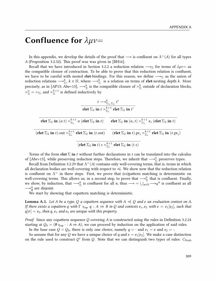
APPENDIX A
Confluence for λµν=
In this appendix, we develop the details of the proof that −→ is confluent on Λ=(A) for all typesA (Proposition 3.2.32). This proof was was given in [BH16].
Recall that we have introduced in Section 3.2.2 a reduction relation −→Σ for terms of λµν= asthe compatible closure of contraction. To be able to prove that this reduction relation is confluent,we have to be careful with nested rlet-bindings. For this reason, we define −→Σ as the union ofreduction relations −→k
Σ, k ∈ N, where −→kΣ is a relation on terms of rlet-nesting depth k . More
precisely, as in [AP13; Abe+13], −→kΣ is the compatible closure of ≻kΣ outside of declaration blocks,
≻0Σ = ≻Σ, and ≻k+1Σ is defined inductively by
t −→kΣ1,Σ2
t ′
rlet Σ2 in t ≻k+1Σ1
rlet Σ2 in t ′
rlet Σ2 in (α t) ≻k+1Σ1
α (rlet Σ2 in t) rlet Σ2 in (κi t) ≻k+1Σ1
κi (rlet Σ2 in t)
(rlet Σ2 in t).out ≻k+1Σ1
rlet Σ2 in (t .out) (rlet Σ2 in t).pri ≻k+1Σ1
rlet Σ2 in (t .pri )
(rlet Σ2 in t) s ≻k+1Σ1
rlet Σ2 in (t s)
Terms of the form rletΣ in t without further declarations in t can be translated into the calculusof [Abe+13], while preserving reduction steps. Therefore, we inherit that −→0
Σ preserves types.Recall from Definition 3.2.29 that Λ=(A) contains only well-covering terms, that is, terms in which
all declaration bodies are well-covering with respect to ◁|. We show now that the reduction relationis confluent on Λ= in three steps. First, we prove that (co)pattern matching is deterministic onwell-covering terms. This allows us, in a second step, to prove that −→0
Σ that is confluent. Finally,we show, by induction, that −→n
Σ is confluent for all n, thus −→ =∪
n∈N −→∅n is confluent as all−→n
∅ are disjoint.We start by showing that copattern matching is deterministic.
Lemma A.1. Let A be a type, Q a copattern sequence with A ◁| Q and e an evaluation context on A.If there exists a copattern q with Γ ⊢cop q : A ⇒ B in Q and contexts e1, e2 with e = e1[e2], such thatq[σ ] = e2, then q, e1 and e2 are unique with this property.
Proof. Since any copattern sequence Q covering A is constructed using the rules in Definition 3.2.24starting at Q0 = (∅ ⊢cop · : A⇒ A), we can proceed by induction on the application of said rules.
In the base case Q = Q0, there is only one choice, namely q = · and e1 = e and e2 = ·.So assume that for any Q we have a unique choice of q and e = e1[e2]. We make a case distinction
on the rule used to construct Q ′ from Q . Note that we can distinguish two types of rules: CProd,
309
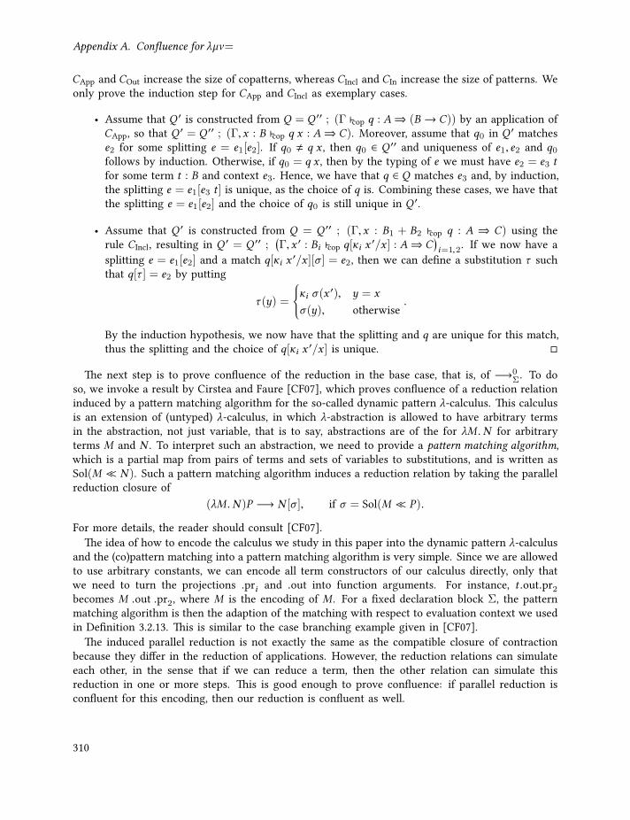
Appendix A. Confluence for λµν=
CApp and COut increase the size of copatterns, whereas CIncl and CIn increase the size of patterns. Weonly prove the induction step for CApp and CIncl as exemplary cases.
• Assume that Q ′ is constructed from Q = Q ′′ ; (Γ ⊢cop q : A⇒ (B → C)) by an application ofCApp, so that Q ′ = Q ′′ ; (Γ,x : B ⊢cop q x : A⇒ C). Moreover, assume that q0 in Q ′ matchese2 for some splitting e = e1[e2]. If q0 , q x , then q0 ∈ Q ′′ and uniqueness of e1, e2 and q0follows by induction. Otherwise, if q0 = q x , then by the typing of e we must have e2 = e3 tfor some term t : B and context e3. Hence, we have that q ∈ Q matches e3 and, by induction,the splitting e = e1[e3 t ] is unique, as the choice of q is. Combining these cases, we have thatthe splitting e = e1[e2] and the choice of q0 is still unique in Q ′.
• Assume that Q ′ is constructed from Q = Q ′′ ; (Γ,x : B1 + B2 ⊢cop q : A ⇒ C) using therule CIncl, resulting in Q ′ = Q ′′ ;
(Γ,x ′ : Bi ⊢cop q[κi x ′/x ] : A⇒ C
)i=1,2
. If we now have asplitting e = e1[e2] and a match q[κi x
′/x ][σ ] = e2, then we can define a substitution τ suchthat q[τ ] = e2 by putting
τ (y) =
κi σ(x
′), y = x
σ(y), otherwise.
By the induction hypothesis, we now have that the splitting and q are unique for this match,thus the splitting and the choice of q[κi x ′/x ] is unique.
The next step is to prove confluence of the reduction in the base case, that is, of −→0Σ. To do
so, we invoke a result by Cirstea and Faure [CF07], which proves confluence of a reduction relationinduced by a pattern matching algorithm for the so-called dynamic pattern λ-calculus. This calculusis an extension of (untyped) λ-calculus, in which λ-abstraction is allowed to have arbitrary termsin the abstraction, not just variable, that is to say, abstractions are of the for λM .N for arbitraryterms M and N . To interpret such an abstraction, we need to provide a pattern matching algorithm,which is a partial map from pairs of terms and sets of variables to substitutions, and is written asSol(M ≪ N ). Such a pattern matching algorithm induces a reduction relation by taking the parallelreduction closure of
(λM .N )P −→ N [σ ], if σ = Sol(M ≪ P).
For more details, the reader should consult [CF07].The idea of how to encode the calculus we study in this paper into the dynamic pattern λ-calculus
and the (co)pattern matching into a pattern matching algorithm is very simple. Since we are allowedto use arbitrary constants, we can encode all term constructors of our calculus directly, only thatwe need to turn the projections .pri and .out into function arguments. For instance, t .out.pr2becomes M .out .pr2, where M is the encoding of M . For a fixed declaration block Σ, the patternmatching algorithm is then the adaption of the matching with respect to evaluation context we usedin Definition 3.2.13. This is similar to the case branching example given in [CF07].
The induced parallel reduction is not exactly the same as the compatible closure of contractionbecause they differ in the reduction of applications. However, the reduction relations can simulateeach other, in the sense that if we can reduce a term, then the other relation can simulate thisreduction in one or more steps. This is good enough to prove confluence: if parallel reduction isconfluent for this encoding, then our reduction is confluent as well.
310
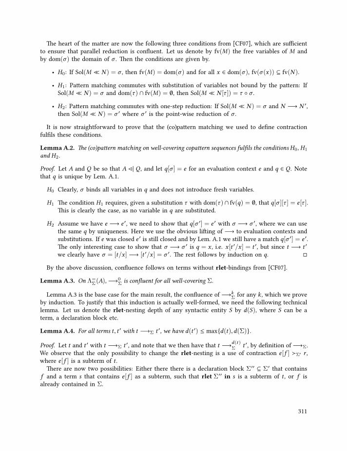
The heart of the matter are now the following three conditions from [CF07], which are sufficientto ensure that parallel reduction is confluent. Let us denote by fv(M) the free variables of M andby dom(σ) the domain of σ . Then the conditions are given by.
• H0: If Sol(M ≪ N ) = σ , then fv(M) = dom(σ) and for all x ∈ dom(σ), fv(σ(x)) ⊆ fv(N ).
• H1: Pattern matching commutes with substitution of variables not bound by the pattern: IfSol(M ≪ N ) = σ and dom(τ ) ∩ fv(M) = ∅, then Sol(M ≪ N [τ ]) = τ σ .
• H2: Pattern matching commutes with one-step reduction: If Sol(M ≪ N ) = σ and N −→ N ′,then Sol(M ≪ N ) = σ ′ where σ ′ is the point-wise reduction of σ .
It is now straightforward to prove that the (co)pattern matching we used to define contractionfulfils these conditions.
Lemma A.2. The (co)pattern matching on well-covering copattern sequences fulfils the conditionsH0, H1
and H2.
Proof. Let A and Q be so that A ◁| Q , and let q[σ ] = e for an evaluation context e and q ∈ Q . Notethat q is unique by Lem. A.1.
H0 Clearly, σ binds all variables in q and does not introduce fresh variables.
H1 The condition H1 requires, given a substitution τ with dom(τ )∩ fv(q) = ∅, that q[σ ][τ ] = e[τ ].This is clearly the case, as no variable in q are substituted.
H2 Assume we have e −→ e ′, we need to show that q[σ ′] = e ′ with σ −→ σ ′, where we can usethe same q by uniqueness. Here we use the obvious lifting of −→ to evaluation contexts andsubstitutions. If e was closed e ′ is still closed and by Lem. A.1 we still have a match q[σ ′] = e ′.The only interesting case to show that σ −→ σ ′ is q = x , i.e. x [t ′/x ] = t ′, but since t −→ t ′
we clearly have σ = [t/x ] −→ [t ′/x ] = σ ′. The rest follows by induction on q.
By the above discussion, confluence follows on terms without rlet-bindings from [CF07].
Lemma A.3. On Λ=Σ(A), −→0
Σ is confluent for all well-covering Σ.
Lemma A.3 is the base case for the main result, the confluence of −→kΣ for any k , which we prove
by induction. To justify that this induction is actually well-formed, we need the following technicallemma. Let us denote the rlet-nesting depth of any syntactic entity S by d(S), where S can be aterm, a declaration block etc.
Lemma A.4. For all terms t , t ′ with t −→Σ t ′, we have d(t ′) ≤ maxd(t),d(Σ).
Proof. Let t and t ′ with t −→Σ t ′, and note that we then have that t −→d(t)Σ t ′, by definition of −→Σ.
We observe that the only possibility to change the rlet-nesting is a use of contraction e[f ] ≻Σ′ r ,where e[f ] is a subterm of t .
There are now two possibilities: Either there there is a declaration block Σ′′ ⊆ Σ′ that containsf and a term s that contains e[f ] as a subterm, such that rlet Σ′′ in s is a subterm of t , or f isalready contained in Σ.
311

Appendix A. Confluence for λµν=
In the first case, we reduce the subterm rletΣ′′ in s to rletΣ′′ in s ′, which induces the reductiont −→Σ t ′ by the compatible closure and the rlet-rules. In turn, this reduction of subterms must begiven by a reduction s −→Σ′ s
′, where Σ′′ ⊆ Σ′, which is then induced by a contraction e[f ] ≻Σ′ rwith (f : A = D) ∈ Σ′′. By definition, we now have d(rlet Σ′′ in s) = maxd(Σ′′) + 1,d(s), thusd(r) ≤ d(D) and d(s ′) ≤ maxd(r),d(s) ≤ maxd(D),d(s). This implies that d(rlet Σ′′ in s ′) =maxd(Σ′′) + 1,d(s ′) ≤ maxd(Σ′′) + 1,d(D),d(s) = d(rletΣ′′ in s), where the last step followsfrom (f : A = D) ∈ Σ′′. Since the only change caused by the reduction t −→ t ′ happens in s , wehave d(t ′) ≤ d(t).
In the second case, we similarly get that d(r) ≤ d(Σ). Together with the first case, we have thatd(r) ≤ maxd(t),d(Σ).
This result allows us to prove that −→kΣ is confluent using induction on k , as the nesting depth
cannot be increased by reduction steps.
Proof of Proposition 3.2.32. We show that −→kΣ is confluent by induction on k , which implies that
−→Σ is confluent because every term has a unique rlet-depth. This induction is well-founded byLem. A.4. The base case is dealt with in Lem. A.3, so we immediately continue with the inductionstep.
Assume that −→kΣ is confluent for any well-covering Σ, we show that for any well-covering Σ
the relation −→k+1Σ confluent. As usual, we show that for terms t , t1 and t2 with t −→k+1
Σ ti thereis a term t3 with ti
k+1Σ t3, which is called weak confluence and implies confluence. First, we
note that if the reductions to t1 and t2 both come from the compatible closure, then we can find t3by induction on the definition of the compatible closure. The base case of this induction requiresthe existence of t3 for the case where t −→k+1
Σ t1 and t ≻k+1Σ t2, which we prove in the following.
i) If t = rlet Σ′ in s , then we have the following cases.a) ti = rletΣ′ in si with s −→k
Σ,Σ′ si . Since −→kΣ,Σ′ is confluent by induction, there is an
s3 with si −→kΣ,Σ′ s3 and we can join t1 and t2 with rlet Σ in s3.
b) t1 = rlet Σ′ in s1 with s −→kΣ,Σ′ s1, s = α s ′ and t2 = α (rlet Σ′ in s ′). Then we must
have that s1 = α s ′1 with s1 −→kΣ,Σ′ s
′1, hence we can t1 and t2 by
t = rlet Σ′ in (α s ′)
t1 = rlet Σ′ in (α s ′1) t2 = α (rlet Σ′ in s ′)
α (rlet Σ′ in s ′1)
c) We proceed analogously if s = κi s′.
d) The other cases follow by symmetry.
ii) If t = (rletΣ′ in s).out, t2 = rletΣ′ in (s .out) and t1 = (rletΣ′ in s1).out with s −→kΣ,Σ′ s1,
then we can reduce t1 to rlet Σ′ in (s1.out) and s to s1. Thus the joining term is rlet Σ′ in(s1.out).
312
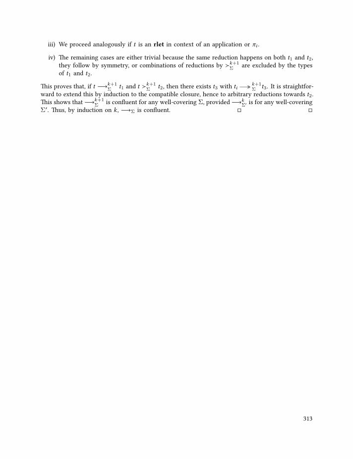
iii) We proceed analogously if t is an rlet in context of an application or πi .
iv) The remaining cases are either trivial because the same reduction happens on both t1 and t2,they follow by symmetry, or combinations of reductions by ≻k+1
Σ are excluded by the typesof t1 and t2.
This proves that, if t −→k+1Σ t1 and t ≻k+1
Σ t2, then there exists t3 with tik+1Σ t3. It is straightfor-
ward to extend this by induction to the compatible closure, hence to arbitrary reductions towards t2.This shows that −→k+1
Σ is confluent for any well-covering Σ, provided −→kΣ′ is for any well-covering
Σ′. Thus, by induction on k , −→Σ is confluent.
313


APPENDIX B
Proofs of Section 6.3
We need the following technical tool.Lemma B.1 (Primitive corecursion). Let C be a category with binary coproducts and F : C → C anendofunctor on C with a final coalgebra (M, ξ : M → FM). For every morphism c : X → F (X +M) inC, there is a unique map h : X +M → M , such that h κ2 = idM and the following diagram commutes.
X M
F (X +M) FM
c
h κ1
ξ
Fh
Proof. We define h as the coinductive extension as in the following diagram.
X X +M M
F (X +M) F (X +M) FM
c
κ1 h
[c,Fκ2ξ ] ξ
Fh
It is easily checked that the rectangle on the right commutes if and only if the above identities hold.Thus uniqueness of h follows from uniqueness of coinductive extensions.
Primitive corecursion allows us to define one-step behaviour as follows.Lemma B.2 (One-step extension). Let F and (M, ξ ) as above, and let f : M → FM be a morphism.Then there exists a unique д : M → M , such that ξ д = f .
Proof. We define д = h κ1, where h arises by primitive corecursion of Fκ2 f . It is then straight-forward to show that ξ д = f if and only the identities of primitive corecursion hold. Thus д isthe unique morphism for which this identity holds.
Using the definition of V as equaliser of u1 and u2, we can characterise elements of V as follows.First we note that V is indexed over I by q = V
д−→ Mf
ρ−→ A
t−→ I , where ρ is the root map givenby composing ξf with projection for coproducts. Abusing notation, we will use V instead of q, andwrite x : Vi if x : V and q x = i .
Let X be an object in B. An object R ∈ B/X 2 is called a relation, and we say that elements x ,y : Xare related by are, denoted (x ,y) : R, if there is a z : R, such that π1(R z) = x and π2(R z) = y.Lemma B.3 (Internal bisimulations). Let f : B → A be a polynomial and R ∈ B/M2
f a relation over Mfsuch that
∀(x1,x2) : R. if ξf (xk ) = (ak ,vk )
then a1 = a2 = a
and (∀b : B. f b = a ⇒ (v1 b,v2 b) : R).
315

Appendix B. Proofs of Section 6.3
Then for all (x1,x2) : R, we have that x1 = x2.
Proof. It is easy to see that this allows us to define a coalgebra structure on R : U → M2f such
that πk R : U → M2 are homomorphism for k = 1, 2, which implies by finality of Mf thatπ1 R = π2 R.
In the following lemmas we use the notation introduced in the proof of Thm. 6.3.6.
Lemma B.4. If y : Mf and b : B such that φ(u1 y,b) = u1 y, then qy = s b and u1 y = u2 y.
Proof. We let ξf y = (a,v) and then find that
ξf ×I (φ(u1 y,b)) = (a, s b, λb ′.φ(u1 (v b′),b ′))
= (a, t a, λb ′.u1 (v b′)) by assumption
= ξf ×I (u1 y).
Thus s b = t a = qy and φ(u1 (v b ′),b ′) = u1 (v b′) for all b ′ : B with f b = a. This gives us
ξf ×I (u1 y) = (a, t a, λb ′.u1 (v b′))
= (a, t a, λb ′.φ(u1 (v b′),b ′)) see above
= ξf ×I (u2 y)
as required.
Lemma B.5. Let i : I and x : Mf , then the following are equivalent
1. x : Vi
2. u1 x = u2 x and q x = i
3. ξf x = (a : A,v : Πf Mf ), t a = i and (∀b : B. f b = a ⇒ v b : Vs b)
4. ξf x = (a : A,v : Πf Mf ), t a = i and v : Πf (s∗V )
Proof. The equivalences 1 ⇐⇒ 2 and 3 ⇐⇒ 4 are the definitions, so let us prove 2 ⇐⇒ 3.We begin by proving 2 ⇒ 3. Let x : Mf with u1 x = u2 x and q x = i . Then we have for
xf x = (a,v) that t a = q x = i ,
ξf ×I (u1 x) = Jf × IK(u1) (pMf (ξf x)) = (a, t a, λb .u1(v b))
and
ξf ×I (u2 x) = Jf × IK(φ) (ΣA×IK (ξf ×I (u1 x)))
= Jf × IK(φ) (ΣA×IK (a, t a, λb .u1 (v b))
= (a, t a, λb .φ(u1 (v b),b)).
By these calculations and Since u1 x = u2 x , we also have for all b : B with f b = a that u1(v b) =φ(u1 (v b),b). Applying Lem. B.4 to y = v b we get that q (v b) = s b and u1 (v b) = u2 (v b), thusv b : Vs b and 3 holds.
316

For the other direction, assume that ξf x = (a : A,v : Πf Mf ), t a = i and (∀b : B. f b = a ⇒ v b :Vs b). We show that u1 x = u2 x by giving a bisimulation R that relates u1 x and u2 x . We put
X = 1+ΣB . s∗V
R : X → Mf ×Mf
R(∗) = (u1 x ,u2 x)
R(b,y) = (u1 y,φ(y,b))
which is a relation over Mf . To prove that R is a bisimulation, there are two cases to consider. First,we have (u1 x ,u2 x) : R. Note that
ξf ×I (u1 x) = (a, t a, λb .u1 (v b))
and
ξf ×I (u2 x) = (a, t a, λb .φ(u1 (v b),b))
so that ρf ×I (u1 x) = (a, t a) = ρf ×I (u1 x). Moreover, we have for all b : B that u1 (v b) andφ(u1 (v b),b) are related by R. For the second case, let b : B and y : Vs b . Then for xf y = (a′,v ′) wehave
ξf ×I (u1 y) = (a′, t a′, λb ′.u1 (v′b ′))
and
ξf ×I φ(y,b) = (a′, s b, λb ′.φ(u1 (v′b ′),b ′)).
Since y : Vs b , we have, by definition, that s b = qy = t a′, thus (a′, t a′) = (a′, s b). Moreover,u1 (v
′b ′) and u1(v′b ′,b ′) are again related by R. Hence, we can conclude that R is a bisimulation,
and so u1 x = u2 x .
Theorem 6.3.6. By Lemma B.5.4, we immediately have that ξf : Mf → Jf K(Mf ) restricts to ξ ′ : V →JPK(V ). To prove that ξ ′ is also final we need another ingredient. We define a natural transformationι : ΣI JPK ⇒ Jf KΣI (where ΣI : B/I → B) for each k : X → I by ιk
(i : I ,a : A,v : Πf (s
∗ k))=
(a, λb .(s b,v b)) where t(a) = i .Now, let k : X → I be in B/I and c : k → JPK(k) be a coalgebra on k . Using ι, we can define a
morphism h as in the following diagram.
ΣIk Mf
Jf K(ΣIk) Jf K(Mf )
ιk ΣI c
h
ξfJf K(h)Thus for i : I and x : X with k(x) = i , and c(x) = (a,v), we have
ξf (h(i,x)) = Jf K(h)(ιk (i,a,v)) = (a, λb .h(s b,v b)). (B.1)
317

Appendix B. Proofs of Section 6.3
Using (B.1), we can now show that h(k x ,x) : Vk x for x : X . For brevity, we put i B k x . ByLemma B.5.3, we need to show that for ξf (h(i,x)) = (a, λb .h(s b,v b)) with c x = (a,v) we havet a = i and h(s b,v b) : Vs b . The first is immediate, since (a,v) : JPK(k), thus t a = i by definition ofthe extension JPK of P . The second follows by coinduction, as k (v b) = s b.
This allows us to define the coinductive extension c : X → V of c by c x = h(k x ,x) as a morphismk → q in B/I . That c is a homomorphism c → ξ ′ is easily checked as follows.
ξ ′(c x) = ξ ′(h(k x ,x))
= ξf (h(k x ,x))
= (a, λb .h(s b,v b)) (a,v) = c x
= (a, λb .h(k (v b),v b)) k (v b) = s b
= (a, λb .c v b)
= (JPK c)(c x)Finally, we show how uniqueness of c follows from uniqueness of h. Let д : (k, c)→ (q, ξ ′) be aJPK-homomorphism, and define д′ : ΣIk → Mf by д′(i : I ,x : Xi ) = д x . It is easy to see that д′ is aJf K-homomorphism from ιk ΣIc to ξf :
ξf (д′ (i,x)) = ξf (д x)
= (JPKд)(c x) д homomorphism= (a, λb .(s∗ д)(v b)) (a,v) = c x
= (a, λb .д′(s b,v b)) (∗)= (Jf Kд′)(ιk ((ΣIc)(i,x)))
where (∗) follows since v b : Vs b and q(д(v b)) = k(v b) = s b by д being a morphism from k to q.Thus, by finality of ξf , д′ = h and so д = c .
318

Summary
Induction and coinduction are threads that cross the landscape of Mathematics and ComputerScience as methods to define objects and reason about them. Of these two, induction is by far thebetter known technique, although coinduction has always been around in disguise. It was only inrecent years that we began to see through this disguise and developed coinduction as a technique inits own right. This led to some remarkable theory under the umbrella of coalgebra and to strikingapplications of coinduction.
As it turns out, induction and coinduction are complementary techniques, they are dual in aprecise sense. Being complementary, it is often necessary to use both techniques or even intertwinethem. In this thesis, we show that combined induction-coinduction is often used implicitly, just likeinduction and coinduction used to be before they were studied systematically. Thus, the purpose ofthis thesis is to carefully study the combination of induction and coinduction, which hopefully, ifanything, inspires others to work on and use inductive-coinductive techniques.
One example, which pervades the thesis, illustrates the combination particularly well: the so-calledsubstream relation. A stream s, that is an infinite sequence, is a substream of stream t if all theentries of s occur in order in t. Intuitively, one has to find for all entries in s an entry in t with thesame value in finitely many steps. The fact that we may only use a finite number of steps to find eachentry is an iterative process, while its repetition for all entries is a coiterative process. Since thesetwo processes are interleaved, the substream relation is a mixed inductive-coinductive relation.
To be able to deal with such examples, we aim in this thesis to find and study languages for inductive-coinductive definitions and reasoning, which lend themselves to being automatically verifiable, can beequipped with formal semantics, and allow human-readable specifications and proofs. Put in generalterms, the intention of studying languages for inductive-coinductive definitions and reasoning isto provide a framework that is sufficiently rich to accommodate category theory and set theory.Moreover, this framework should allow for semantics that are, in principle, independent of thosetheories, and for proofs that can be formalised and automatically verified. This is of course anambitious goal that will not be fully attained in this thesis, but we will nonetheless contribute to it.
Towards these aims, we proceed in several steps. The first step is to have some objects to reasonabout, which means specifically for this thesis that we provide two programming languages forinductive-coinductive types. In the first language, one can only write terminating programs, while thesecond allows arbitrary recursive specification. Such recursive specifications ease programming withmixed inductive-coinductive types dramatically over programming with the iteration and coiterationschemes in the first language. However, this increased expressiveness also comes at the price thatwe give up simple syntactic conditions for well-defined programs (programs that terminate underany observation) and have to characterise such programs in a different way.
To this end, we establish notions of observationally normalising programs, the well-defined pro-grams, and an observational program equivalence in the presence of inductive-coinductive typesand arbitrary recursive specifications. As it turns out, the characterisation of observationally norm-alising programs is itself an inductive-coinductive predicate. In contrast, the program equivalenceis introduced through a modal logic and turns out to be purely coinductive. Given such a programequivalence, we have to ask whether it is well-motivated. An important property of the equivalence
319

Summary
is that is allows us to construct 2-categories of types and terms, in which equality captures com-putations, while 2-cells represent program equivalences. In particular, least fixed point types andgreatest fixed point types carry, respectively, pseudo-initial algebras and pseudo-final coalgebras inthese 2-categories.
Even though the 2-category theoretical results give us some principles to reason about programs,these principles are not always the most convenient ones to work with. For this reason, we developin the next step more convenient reasoning techniques: a bisimulation proof method, a syntactic first-order logic that is itself recursive, and an algorithm that operates on fragments of the programminglanguages. The bisimulation proof method can be enhanced by using so-called up-to techniques,which we demonstrate by showing that the substream relation is transitive. In particular, we use anup-to technique that allows us to use induction inside a bisimulation proof.
This setup becomes, unfortunately, rather complex because implementing induction as up-totechnique forces a stratification of a mixed inductive-coinductive proof into a coinduction and twoinductions. What is worse, the induction proofs must be proven independently of the coinduction,which makes finding the correct induction hypothesis a highly non-trivial task. To overcome suchproblems, we construe a recursive logic, in which inductive and coinductive proofs are incrementallyconstructed together. Recursion in proofs of this logic is thereby controlled through the so-calledlater modality. This modality allows us to ensure the correctness of a proof through each proof ruleseparately, which makes both proof checking and the soundness proof easy to implement.
Up to this point, the thesis is about programming with simple types, and reasoning about a veryspecific inductive-coinductive predicate (observational normalisation) and a very specific coinductiverelation (observational equivalence). Both are defined in naive set theory, which means that neitherare given in a principled manner nor that proofs about them can be directly formally expressed.This clearly violates our aims and is what caused us to invent, for example, a new logic from scratch.The remainder of the thesis deals with this issue in that we develop a category theoretic and a typetheoretic approach that allow us to formally express results about simple inductive-coinductive types,and inductive-coinductive predicates and relations. It turns out that inductive-coinductive predicatesand relations are best expressed as certain dialgebras in fibrations. This approach subsumes simpletypes and general dependent types. What is more, we are able to define a class of strictly positivedependent types and reduce them to initial algebras and final coalgebras of polynomial functors. Thisreduction to minimal requirement allows us to interpret dependent types in well-studied models.The category theoretical approach to dependent types is concluded by an analysis of the logicalprinciples that are available in a fibration that is closed under strictly positive dependent types.
Following the guiding principles of the category theoretical development, we construct also a(syntactic) dependent type theory. This results in a small type theory that is merely based oninductive-coinductive dependent types, yet it admits all basic logical operators like conjunction,implication, quantification etc. Since this type theory is built on iteration and coiteration principles,we are able to show that all terms in that theory are strongly normalising. The thesis is concludedby giving a general induction principle for this type theory and an elaborate example of inductive-coinductive reasoning in Agda.
320
Samenvatting
Inductie en coinductie vormen twee technieken in het landschap van Wiskunde en Informaticadie gebruikt worden om objecten te definiëren en om eigenschappen van deze objecten te laten zien.Inductie is bekender dan coinductie, maar coinductie was er op de achtergrond ook altijd al. In delaatste jaren is men begonnen coinductie als een op zich zelf staande techniek te ontwikkelen. Inhet kader van coalgebra is daar een uitgebreide theorie met opmerkelijke toepassingen uitgekomen.
Het blijkt dat inductie en coinductie complementair zijn: ze zijn op een bepaalde manier duaal.Omdat dat ze complementair zijn, moeten beide technieken vaak samen gebruikt worden. In ditproefschrift laten wij zien dat dit vaak impliciet gebeurt, op dezelfde manier als inductie en coinductievroeger impliciet gebruikt werden voordat ze systematisch bestudeerd werden. Het doel van ditproefschrift is dus de combinatie van inductie en coinductie in detail te bestuderen, wat hopelijkinspiratie geeft om inductieve/coinductieve technieken verder te ontwikkelen en te gebruiken.
Een voorbeeld, die als een rode draad door dit proefschrift loopt en de combinatie verduidelijkt,is de zogenaamde deelstroomrelatie. Die relateert stromen, dus oneindige rijen, s and t dan enslechts dan als alle elementen in s in dezelfde volgorde in t voorkomen. De intuïtie is dat we vooriedere positie in s een element met dezelfde waarde in t moeten vinden, in eindig veel stappen. Hetfeit dat wij slechts eindig veel stappen mogen gebruiken om de positie te vinden, maakt het eeniteratief proces, terwijl de herhaling een coiteratief proces is. Omdat deze twee processen van elkaarafhankelijk zijn, is de deelstroomrelatie een gemengde inductieve/coinductieve relatie.
Om met dit soort voorbeelden om te kunnen gaan, bestuderen en zoeken we in dit proefschrift ta-len voor inductieve/coinductieve definities en eigenschappen, die als basis voor de automatische verificatievan bewijzen gebruikt kunnen worden, die een formele semantiek hebben, en die makkelijk inzetbaar zijndoor anderen. Vanuit een abstract perspectief is het doel van deze studie van inductieve/coinductievedefinities en bewijsprincipes het geven van een raamwerk dat als logische basis voor categorieën-theorie een verzamelingstheorie kan dienen. Verder moet het mogelijk zijn een semantiek voor ditraamwerk te geven, die in beginsel onafhankelijk van deze theorieën is, en moet het mogelijk zijnbewijzen uit dit raamwerk te formaliseren en automatisch te verifiëren. Dit is een ambitieus doeldat niet geheel gehaald kan worden in dit proefschrift, maar waartoe we zeker een bijdrage leveren.
We gaan in meerdere stappen te werk om in richting van de bovengenoemde doelen te gaan.De eerste stap is dat we objecten nodig hebben waarvan we eigenschappen willen beschrijven. Indit proefschrift betekent dit specifiek dat wij twee talen voor het programmeren met inductieve encoinductieve typen introduceren. In de eerste taal is het mogelijk alleen convergerende programma’sop te schrijven, terwijl de tweede taal willekeurige, recursieve specificaties toestaat. Zulke recursievespecificaties maken het programmeren met gemengde inductieve/coinductieve typen veel makkelij-ker, vergeleken met het programmeren met iteratie- en coiteratieschema’s in de eerste taal. Hetprobleem met algemene recursie is dat wij eenvoudige, syntactische condities voor welgedefinieerdeprogramma’s—die bij het toepassen van iedere observatie termineren—verliezen en dat we dezeprogramma’s op een andere manier moeten karakteriseren.
Om dit te bereiken, introduceren we een begrip van welgedefinieerde programma’s, dat we “ob-servationally normalising” noemen, en een programma-equivalentie in de context van inductie-ve/coinductieve typen en algemene recursieve specificaties. Het blijkt dat de karakterisering van
321

Samenvatting
welgedefinieerde programma’s zelf een inductief/coinductief predicaat is. Daarentegen wordt de pro-grammaequivalentie als een modale logica geïntroduceerd, en is deze equivalentie puur coinductief.Om een goede motivatie voor deze programmaequivalentie te geven, introduceren we een 2-categorievan typen, termen en equivalenties als 2-cellen. In deze 2-categorie komen kleinste fixpunten overeenmet pseudo-initiële algebra’s, en grootste fixpunten met pseudo-finale coalgebra’s.
Hoewel we bepaalde technieken uit 2-categorieëntheoretische resultaten kunnen halen, zijn dezetechnieken niet altijd het meest geschikt. Daarom ontwikkelen wij in een volgende stap praktischerebewijsmethoden: een methode gebaseerd op bisimulaties, een syntactische, recursieve eerste-ordelogica, en een algoritme voor een fragment van de programmeertalen. De bisimulatieaanpak kandoor zogenaamde up-to technieken verbeterd worden. Wij demonstreren dit door een voorbeeld,waarin we laten zien dat de deelstroomrelatie transitief is. Daarbij maken maken wij vooral gebruikvan een up-to techniek waarmee we inductie in een bisimulatiebewijs kunnen gebruiken.
Deze opzet wordt helaas best ingewikkeld, omdat door de implementatie van inductie als up-techniek een stratificatie van een gemengd inductief/coinductief bewijs in een coinductie en tweeinducties gebeurt. Sterker nog, de inductieve bewijzen moeten onafhankelijk van de coinductievestap bewezen worden, waardoor het vinden van de juiste inductiehypotheses zelf een ingewikkeldeopgave wordt. Om dit probleem op te lossen, ontwikkelen we een recursieve logica waarin inductieveen coinductieve bewijzen samen en incrementeel geconstrueerd worden. Om te voorkomen dat derecursie in bewijzen misgaat, gebruiken wij de zogenaamde “later modality”. Omdat het door dezemodaliteit mogelijk is de correctheid van bewijzen op het niveau van regels te waarborgen, wordenook het controleren van bewijzen en het correctheidsbewijs vereenvoudigd.
Tot dit punt gaat het in het proefschrift alleen maar over het programmeren met eenvoudige typen,en over eigenschappen van een specifiek inductief/coinductief predicaat (observational normalisa-tion) en een specifieke coinductieve relatie (observational equivalence). Beide zijn in een naïeveverzamelingstheorie gedefinieerd, dus zijn deze definities niet op fundamentele principes gebaseerd,en kunnen bewijzen over dit predicaat/deze relatie niet direct formeel uitgedrukt worden. Dit gaattegen onze doelen in, en is een reden om de recursieve logica te ontwikkelen. In het resterende deelvan het proefschrift lossen we dit op door categorieëntheoretische en typentheoretische aanpakkente ontwikkelen die het mogelijk maken resultaten over eenvoudige inductieve/coinductieve typen,predicaten en relaties formeel uit te drukken. Het blijkt dat dialgebra’s in vezelingen de beste manierzijn om inductieve/coinductieve predicaten en relaties uit te drukken. Door deze aanpak wordt hetook mogelijk met eenvoudige typen en algemene afhankelijke typen om te gaan. Bovendien kun-nen wij een klasse van strikt positieve, afhankelijke typen definiëren, waarvoor wij een semantiekin vorm van initiële algebra’s en finale coalgebra’s van polynomiale functoren krijgen. Door dezereductie naar minimale eisen wordt het mogelijk afhankelijke typen over welbekende modellen te in-terpreteren. We sluiten de categorieëntheoretische aanpak af met een analyse van logische principesdie gelden in een vezeling die gesloten is onder strikt positieve, afhankelijke typen.
De laatste stap is de constructie van een (syntactische) afhankelijke typentheorie, waarbij wij deprincipes van de categorieëntheoretische aanpak volgen. Daardoor krijgen wij een typentheoriemet weinig regels die alleen maar op inductieve/coinductieve, afhankelijke typen gebaseerd is, maarnog steeds logische operatoren zoals conjunctie, implicatie en kwantificering toestaat. Omdat dezetypentheorie alleen op iteratie en coiteratie gebaseerd is kunnen wij laten zien dat alle termen indeze theorie sterk-normaliserend zijn. We sluiten het proefschrift met een algemeen inductieprincipevoor deze typentheorie en een uitgebreid voorbeeld van een inductief/coinductief bewijs in Agda.
322

Zusammenfassung
Induktion und Koinduktion ziehen sich durch die mathematische und informatische Landschaftwie zwei Ströme, die genutzt werden um Objekte zu definieren und Eigenschaften dieser Objekteherzuleiten. Von den beiden Techniken ist Induktion die besser bekannte, obwohl Koinduktion schonimmer, wenn auch implizit, genutzt worden ist. Lediglich in den letzten Jahren wurde Koinduktion alseigenständige Technik entwickelt, wobei sich das Gebiet der sogenannten Koalgebren herausgebildethat. Dieses Gebiet umfasst mittlerweile eine weitläufige Theorie und bemerkenswerte Anwendungen.
Es hat sich herausgestellt, dass Induktion und Koinduktion komplementäre Techniken sind: umgenau zu sein, sind sie dual. Da sie komplementär sind, ist es häufig notwendig beide Technikenzusammen zu gebrauchen. In dieser Dissertation zeigen wir, dass dies zumeist implizit passiert, ge-nauso wie früher Induktion und Koinduktion implizit genutzt worden sind, bevor sie systematischuntersucht worden sind. Der Zweck dieser Dissertation ist daher systematisch und im Detail dieKombination von Induktion und Koinduktion zu untersuchen. Falls irgendetwas aus dieser Disserta-tion hervorgeht, dann dass sie hoffentlich andere inspiriert induktiv-koinduktive Techniken weiterzu entwickeln und zu gebrauchen.
Ein Beispiel, das sich als roter Faden durch diese Arbeit zieht und das die Kombination vonInduktion und Koinduktion verdeutlicht, ist die sogenannte Teilstromrelation. In dieser Relationstehen Ströme (unendliche Folgen) s und t genau dann in Beziehung, wenn alle Einträge in s in dergleichen Reihenfolge in t auftauchen. Die Intuition dieser Beziehung ist, dass wir für jede Positionin s mit Gebrauch von endlich vielen Schritten einen Eintrag in t mit dem gleichen Wert findenmüssen. Tatsächlich ist die Suche in endlich vielen Schritten ein iterativer Prozess, wohingegen ihreWiederholung für jede Position ein koiterativer Prozess ist. Da diese beiden Prozessen verzahnt sind,ist die Teilstromrelation eine gemischt induktiv-koinduktive Relation.
Um mit derartigen Beispielen umgehen zu können, untersuchen wir in dieser Arbeit Sprachen fürinduktiv-koinduktive Definitionen und Eigenschaften, welche als Basis für die automatische Verifikationvon Beweisen genutzt werden können, welche eine formale Semantik haben, und welche es ermögli-chen Spezifikationen und Beweise derart zu formulieren, dass diese für Menschen verständlich sind. Ausder Vogelperspektive ist das Ziel unserer Untersuchungen von induktiv-koinduktiven Definitionenund Beweisen das Schaffen eines Rahmens, welcher als logisches Fundament für Kategorien- undMengentheorie fungieren kann. Außerdem muss es möglich sein, diesem Rahmen eine Interpretationzu geben, die im Prinzip unabhängig von diesen Theorien ist und es muss möglich sein die Beweise,die in diesem Rahmen gegeben werden, zu formalisieren. Das ist ein ehrgeiziges Ziel, das wir indieser Arbeit nicht erreichen, und doch werden wir sicher einen Beitrag in diese Richtung leisten.
Um die genannten Ziele zu erreichen, werden wir in mehreren Schritten vorgehen. Zunächstbenötigen wir Objekte, über die wir Aussagen treffen können. In dieser Arbeit bedeutet das imSpeziellen, dass wir zwei Programmiersprachen zum Programmieren mit induktiven und koinduk-tiven Typen entwickeln. In der ersten Sprache können nur terminierende Programme beschriebenwerden, während die zweite Sprache beliebige rekursive Programme zulässt. Im Vergleich zu denIterations- und Koiterationsschemata der ersten Sprache, wird das Programmieren durch das Erlau-ben beliebiger Rekursionen immens vereinfacht. Allerdings ist der Preis, den wir für die stärkereAusdruckskraft zahlen müssen, dass es nicht mehr möglich ist wohldefinierte Programme, die unter
323

Zusammenfassung
jeder Beobachtung terminieren, durch einfache syntaktische Kriterien zu charakterisieren.Um eine solche Charakterisierung dennoch zu erreichen und umAussagen über induktiv-koinduktive
Programme mit beliebiger Rekursion treffen zu können, führen wir einen Begriff von wohldefiniertenProgrammen, die wir “observationally normalising” nennen, und eine Programmäquivalenz ein. Esstellt sich heraus, dass die Charakterisierung von wohldefinierten Programmen selbst ein induktiv-koinduktives Prädikat ist. Dahingegen ist die Programmäquivalenz durch eine Modallogik gegebenund rein koinduktiv. Um die Programmäquivalenz zu motivieren, definieren wir eine 2-Kategorie,bestehend aus Typen als Objekte, Programmen als Morphismen und Programmäquivalenzen als2-Zellen. In dieser 2-Kategorie werden Berechnungen durch Gleichungen zwischen Morphismenrepräsentiert, während herleitbare Programmäquivalenzen Isomorphismen von Morphismen sind.Im Speziellen zeigen wir, dass kleinste Fixpunkttypen mit pseudo-initialen Algebren und größteFixpunkttypen mit pseudo-finalen Koalgebren zusammenfallen.
Auch wenn die Resultate über 2-Kategorien uns bereits einige Prinzipien geben, um Beweiseüber Programme zu führen, ist dieser Ansatz nicht immer der geeignetste. Daher entwickeln wir imFolgenden praktischere Beweistechniken: eine auf Bisimulationen basierte Methode, eine syntaktischePrädikatenlogik erster Stufe mit rekursiven Beweisen, und einen Algorithmus, der die Äquivalenzfür ein Fragment der Programmiersprachen entscheiden kann. Die Bisimulationenmethode kanndurch sogenannte up-to-Techniken verbessert werden. Wir führen dies anhand eines Beispiels vor,in welchem wir zeigen, dass die Teilstromrelation transitiv ist. Hierbei benutzen wir vor allem eineup-to-Technik, durch welche wir Induktion innerhalb eines Bisimulationsbeweis gebrauchen können.
Leider wird dieser Ansatz ziemlich komplex, da die Umsetzung von Induktion als up-to-Technikeinen gemischt induktiv-koinduktiven Beweis in eine Koinduktion und zwei Induktionen schichtet.Schwerer wiegt aber, dass die induktiven Beweise unabhängig von dem koinduktiven Schritt geführtwerden müssen, wodurch das Finden der richtigen Induktionsannahme selbst zu einer schwierigenAufgabe wird. Um dieses Problem zu lösen, entwickeln wir eine rekursive Logik, in der induktiveund koinduktive Beweise zusammen und inkrementell konstruiert werden. Rekursion wird in dieserLogik durch die sogenannte “later modality” kontrolliert. Mit Hilfe dieser Modalität können wir dieKorrektheit von formalen Beweisen in jedem Beweisschritt einzeln sicherstellen, wodurch das Prüfenvon Beweisen und der Korrektheitsbeweis für die Logik relativ einfach werden.
Bis hierin geht es in der Dissertation allein um das Programmieren mit einfachen Typen, undum Eigenschaften eines spezifischen induktiv-koinduktiven Prädikates (observational normalisation)und einer spezifischen koinduktiven Relation (observational equivalence). Beide sind in naiver Men-genlehre definiert, das heißt, dass ihre Definitionen weder auf fundamentalen Prinzipien basierennoch, dass Aussagen über sie direkt formalisiert werden können. Dies widerspricht unseren Zielenund ist einer der Gründe, warum wir die rekursive Logik entwickeln mussten. Im übrigen Teil derDissertation lösen wir dieses Problem auf, indem wir kategorientheoretische und typentheoretischeAnsätze entwickeln, welche es uns erlauben Aussagen über induktiv-koinduktive Typen, Prädikateund Relationen formal auszudrücken. Dabei stellt sich heraus, dass induktiv-koinduktive Prädikateund Relationen am besten als sogenannte Dialgebren in Faserkategorien präsentiert werden. DieserAnsatz erlaubt es uns mit einfachen und abhängigen Typen umzugehen. Darüber hinaus können wirin diesem Aufbau eine Klasse von strikt positiven, abhängigen Typen definieren, für die wir eineInterpretation durch initiale Algebren und finale Koalgebren von polynomiellen Funktoren angebenkönnen. Durch dies Reduktion auf minimale Anforderungen wird es möglich, unsere abhängigenTypen in wohlbekannten Modellen zu interpretieren. Wir schließen den kategorientheoretischen
324

Ansatz mit einer Analyse der logischen Prinzipien, die aus einer, unter strikt positiven abhängigenTypen abgeschlossenen, Faserkategorie hervorgehen.
Im letzten Schritt konstruieren wir, den Prinzipien des kategorientheoretischen Ansatzes fol-gend, eine (syntaktische) abhängige Typentheorie. Daraus resultiert eine Typentheorie, die alleinauf induktiv-koinduktiven Typen basiert ist und die mit wenigen Schlussregeln auskommt, in deraber trotzdem alle Operatoren (Konjunktion, Implikation,Quantoren etc.) einer Prädikatenlogik ersterStufe ausgedrückt werden können. Da diese Typentheorie ausschließlich auf Iteration und Koiterati-on basiert, können wir zeigen, dass jede Reduktion zu einer Normalform führt. Dies stellt, zusammenmit Konfluenz und kanonischen Normalformen, die Konsistenz der Typentheorie als Logik sicher.Wir schließen die Dissertation mit einem allgemeinen Induktionsprinzip für diese Typentheorie undeinem ausführlichen Beispiel eines induktiv-koinduktiven Beweises in Agda.
325


Curriculum Vitae
2000 – 2006 Abitur (university entrance qualification), Grammar school Gaußschule, Braun-schweig.
2006 – 2007 Alternative Civilian Service, Umweltinformations- und Innovationszentrum(Centre for environment information and innovation), Städtisches KlinikumBraunschweig.
2007 – 2011 Software development for train control and communication system, BBR Verkehrs-technik, Braunschweig.
2007 – 2010 Bachelor Computer Science, TU Braunschweig, Bachelor’s Thesis: Parallelisminvestigation for elliptic curve key exchange, Institute of Computer and NetworkEngineering.
2011 – 2012 Research Assistant: Project VerSyKo Institute of Theoretical Computer Science,TU Braunschweig, Supervised by Stefan Milius.
2010 – 2012 Master Computer Science, TU Braunschweig, Master’s Thesis: Transformation ofSCADE models for SMT based verification, Institute of Theoretical ComputerScience.
2012 – 2013 Internship: Research on coalgebra-based descriptions of systems, CWI (Centre forMathematics and Computer Science), Amsterdam, Supervised by Marcello Bon-sague and Jan Rutten.
2013 – 2017 PhD Computer Science, Radboud University, Nijmegen. Thesis Title: MixedInductive-Coinductive Reasoning – Types, Programs and Logic.
2017 – Post-Doc, PLUME Team of the LIP, ENS Lyon, CNRS.
327
Titles in the IPA Dissertation Series since 2015
G. Alpár. Attribute-Based Identity Management:Bridging the Cryptographic Design of ABCs withthe Real World. Faculty of Science, Mathematicsand Computer Science, RU. 2015-01
A.J. van der Ploeg. Efficient Abstractions forVisualization and Interaction. Faculty of Science,UvA. 2015-02
R.J.M. Theunissen. Supervisory Control inHealth Care Systems. Faculty of Mechanical En-gineering, TU/e. 2015-03
T.V. Bui. A Software Architecture for Body AreaSensor Networks: Flexibility and Trustworthiness.Faculty of Mathematics and Computer Science,TU/e. 2015-04
A. Guzzi. Supporting Developers’ Teamworkfrom within the IDE. Faculty of Electrical En-gineering, Mathematics, and Computer Science,TUD. 2015-05
T. Espinha. Web Service Growing Pains: Under-standing Services and Their Clients. Faculty ofElectrical Engineering, Mathematics, and Com-puter Science, TUD. 2015-06
S. Dietzel. Resilient In-network Aggregation forVehicular Networks. Faculty of Electrical En-gineering, Mathematics & Computer Science,UT. 2015-07
E. Costante. Privacy throughout the Data Cycle.Faculty of Mathematics and Computer Science,TU/e. 2015-08
S. Cranen. Getting the point — Obtaining andunderstanding fixpoints in model checking. Fac-ulty of Mathematics and Computer Science,TU/e. 2015-09
R. Verdult. The (in)security of proprietary cryp-tography. Faculty of Science, Mathematics andComputer Science, RU. 2015-10
J.E.J. de Ruiter. Lessons learned in the analysisof the EMV and TLS security protocols. Faculty
of Science, Mathematics and Computer Science,RU. 2015-11Y. Dajsuren. On the Design of an ArchitectureFramework and Quality Evaluation for Automot-ive Software Systems. Faculty of Mathematicsand Computer Science, TU/e. 2015-12J. Bransen. On the Incremental Evaluation ofHigher-Order Attribute Grammars. Faculty ofScience, UU. 2015-13S. Picek. Applications of Evolutionary Computa-tion to Cryptology. Faculty of Science, Mathem-atics and Computer Science, RU. 2015-14C. Chen. Automated Fault Localization forService-Oriented Software Systems. Faculty ofElectrical Engineering, Mathematics, and Com-puter Science, TUD. 2015-15S. te Brinke. Developing Energy-Aware Software.Faculty of Electrical Engineering, Mathematics& Computer Science, UT. 2015-16R.W.J. Kersten. Software Analysis Methodsfor Resource-Sensitive Systems. Faculty of Sci-ence, Mathematics and Computer Science,RU. 2015-17J.C. Rot. Enhanced coinduction. Faculty of Math-ematics and Natural Sciences, UL. 2015-18M. Stolikj. Building Blocks for the Internet ofThings. Faculty of Mathematics and ComputerScience, TU/e. 2015-19D. Gebler. Robust SOS Specifications of Probabil-istic Processes. Faculty of Sciences, Departmentof Computer Science, VUA. 2015-20M. Zaharieva-Stojanovski. Closer to ReliableSoftware: Verifying functional behaviour of con-current programs. Faculty of Electrical En-gineering, Mathematics & Computer Science,UT. 2015-21R.J. Krebbers. The C standard formalized in Coq.Faculty of Science, Mathematics and ComputerScience, RU. 2015-22

R. van Vliet. DNA Expressions – A Formal Nota-tion for DNA. Faculty of Mathematics and Nat-ural Sciences, UL. 2015-23
S.-S.T.Q. Jongmans. Automata-Theoretic Pro-tocol Programming. Faculty of Mathematics andNatural Sciences, UL. 2016-01
S.J.C. Joosten. Verification of Interconnects. Fac-ulty of Mathematics and Computer Science,TU/e. 2016-02
M.W. Gazda. Fixpoint Logic, Games, and Rela-tions of Consequence. Faculty of Mathematicsand Computer Science, TU/e. 2016-03
S. Keshishzadeh. Formal Analysis and Verific-ation of Embedded Systems for Healthcare. Fac-ulty of Mathematics and Computer Science,TU/e. 2016-04
P.M. Heck. Quality of Just-in-Time Require-ments: Just-Enough and Just-in-Time. Faculty ofElectrical Engineering, Mathematics, and Com-puter Science, TUD. 2016-05
Y. Luo. From Conceptual Models to Safety Assur-ance – Applying Model-Based Techniques to Sup-port Safety Assurance. Faculty of Mathematicsand Computer Science, TU/e. 2016-06
B. Ege. Physical Security Analysis of EmbeddedDevices. Faculty of Science, Mathematics andComputer Science, RU. 2016-07
A.I. van Goethem. Algorithms for CurvedSchematization. Faculty of Mathematics andComputer Science, TU/e. 2016-08
T. van Dijk. Sylvan: Multi-core Decision Dia-grams. Faculty of Electrical Engineering, Math-ematics & Computer Science, UT. 2016-09
I. David. Run-time resource management forcomponent-based systems. Faculty of Mathem-atics and Computer Science, TU/e. 2016-10
A.C. van Hulst. Control Synthesis using ModalLogic and Partial Bisimilarity – A Treatise Suppor-ted by Computer Verified Proofs. Faculty of Mech-anical Engineering, TU/e. 2016-11
A. Zawedde. Modeling the Dynamics of Require-ments Process Improvement. Faculty of Mathem-atics and Computer Science, TU/e. 2016-12
F.M.J. van den Broek. Mobile CommunicationSecurity. Faculty of Science, Mathematics andComputer Science, RU. 2016-13
J.N. van Rijn. Massively Collaborative MachineLearning. Faculty of Mathematics and NaturalSciences, UL. 2016-14
M.J. Steindorfer. Efficient Immutable Collec-tions. Faculty of Science, UvA. 2017-01
W. Ahmad. Green Computing: Efficient EnergyManagement of Multiprocessor Streaming Applic-ations via Model Checking. Faculty of ElectricalEngineering, Mathematics & Computer Science,UT. 2017-02
D. Guck. Reliable Systems – Fault tree analysisvia Markov reward automata. Faculty of Elec-trical Engineering, Mathematics & ComputerScience, UT. 2017-03
H.L. Salunkhe. Modeling and Buffer Ana-lysis of Real-time Streaming Radio ApplicationsScheduled on Heterogeneous Multiprocessors. Fac-ulty of Mathematics and Computer Science,TU/e. 2017-04
A. Krasnova. Smart invaders of private mat-ters: Privacy of communication on the Internetand in the Internet of Things (IoT). Faculty ofScience, Mathematics and Computer Science,RU. 2017-05
A.D. Mehrabi. Data Structures for AnalyzingGeometric Data. Faculty of Mathematics andComputer Science, TU/e. 2017-06
D. Landman. Reverse Engineering Source Code:Empirical Studies of Limitations and Opportunit-ies. Faculty of Science, UvA. 2017-07
W. Lueks. Security and Privacy via Crypto-graphy – Having your cake and eating it too. Fac-ulty of Science, Mathematics and Computer Sci-ence, RU. 2017-08

Curriculum Vitae
A.M. Şutîi. Modularity and Reuse of Domain-Specific Languages: an exploration with MetaMod.Faculty of Mathematics and Computer Science,TU/e. 2017-09U. Tikhonova. Engineering the Dynamic Se-mantics of Domain Specific Languages. Fac-ulty of Mathematics and Computer Science,TU/e. 2017-10Q.W. Bouts. Geographic Graph Construction andVisualization. Faculty of Mathematics and Com-puter Science, TU/e. 2017-11A. Amighi. Specification and Verification ofSynchronisation Classes in Java: A Practical Ap-proach. Faculty of Electrical Engineering, Math-ematics & Computer Science, UT. 2018-01S. Darabi. Verification of Program Parallelization.Faculty of Electrical Engineering, Mathematics
& Computer Science, UT. 2018-02
J.R. Salamanca Tellez. Coequations andEilenberg-type Correspondences. Faculty ofScience, Mathematics and Computer Science,RU. 2018-03
P. Fiterău-Broştean. Active Model Learning forthe Analysis of Network Protocols. Faculty ofScience, Mathematics and Computer Science,RU. 2018-04
D. Zhang. From Concurrent State Machines to Re-liable Multi-threaded Java Code. Faculty of Math-ematics and Computer Science, TU/e. 2018-05
H. Basold. Mixed Inductive-Coinductive Reas-oning: Types, Programs and Logic. Faculty ofScience, Mathematics and Computer Science,RU. 2018-06
330