Mission Design and Trajectory Analysis for Inspection of...

Mission Design and Trajectory Analysis for

Inspection of a Host Spacecraft by a Microsatelliteby

Susan C. Kim

S.B., Aerospace EngineeringMassachusetts Institute of Technology (2002)

Submitted to the Department of Aeronautics and Astronauticsin partial fulfillment of the requirements for the degree of

Master of Science in Aeronautics and Astronautics

at the

MASSACHUSETTS INSTITUTE OF TECHNOLOGY

June 2006

c© Susan C. Kim, MMVI. All rights reserved.

The author hereby grants to MIT permission to reproduce anddistribute publicly paper and electronic copies of this thesis document

in whole or in part.

Author . . . . . . . . . . . . . . . . . . . . . . . . . . . . . . . . . . . . . . . . . . . . . . . . . . . . . . . . . . . . . .Department of Aeronautics and Astronautics

May 26, 2006

Certified by. . . . . . . . . . . . . . . . . . . . . . . . . . . . . . . . . . . . . . . . . . . . . . . . . . . . . . . . . .Stanley W. Shepperd

Principal Member of the Technical StaffThe Charles Stark Draper Laboratory, Inc.

Thesis Supervisor

Certified by. . . . . . . . . . . . . . . . . . . . . . . . . . . . . . . . . . . . . . . . . . . . . . . . . . . . . . . . . .David W. Miller

Professor of Aeronautics and AstronauticsThesis Advisor

Accepted by . . . . . . . . . . . . . . . . . . . . . . . . . . . . . . . . . . . . . . . . . . . . . . . . . . . . . . . . .Jaime Peraire

Professor of Aeronautics and AstronauticsChair, Committee on Graduate Students

Mission Design and Trajectory Analysis for Inspection of a

Host Spacecraft by a Microsatellite

by

Susan C. Kim

Submitted to the Department of Aeronautics and Astronauticson May 26, 2006, in partial fulfillment of the

requirements for the degree ofMaster of Science in Aeronautics and Astronautics

Abstract

The trajectory analysis and mission design for inspection of a host spacecraft by amicrosatellite is motivated by the current developments in designing and buildingprototypes of a microsatellite inspector vehicle. Two different mission scenarios arecovered in this thesis – a host spacecraft in orbit about Earth and in deep space. Someof the key factors that affect the design of an inspection mission are presented anddiscussed. For the Earth orbiting case, the range of available trajectories – naturaland forced – is analyzed using the solution to the Clohessy-Wiltshire (CW ) differentialequations. Utilizing the natural dynamics for inspection minimizes fuel costs, whilestill providing excellent opportunities to inspect and image the surface of the hostspacecraft. The accessible natural motions are compiled to form a toolset, which maybe employed in planning an inspection mission. A baseline mission concept for amicrosatellite inspector is presented in this thesis. The mission is composed of fourprimary modes: deployment mode, global inspection mode, point inspection mode,and disposal mode. Some figures of merit that may be used to rate the success of theinspection mission are also presented. A simulation of the baseline mission conceptfor the Earth orbiting scenario is developed from the trajectory toolset. The hardwaresimulation is based on the current microinspector hardware developments at the JetPropulsion Laboratory. Through the figures of merit, the quality of the inspectionmission is shown to be excellent, when the natural dynamics are utilized for trajectorydesign. The baseline inspection mission is also extended to the deep space case.

Thesis Supervisor: Stanley W. ShepperdTitle: Principal Member of the Technical StaffThe Charles Stark Draper Laboratory, Inc.

Thesis Advisor: David W. MillerTitle: Professor of Aeronautics and Astronautics

3

Acknowledgments

Had it not been for the support of the Charles Stark Draper Laboratory (CSDL) and

the Jet Propulsion Laboratory (JPL), this thesis would not have been possible. First,

I would like to thank Stan Shepperd, for his willingness to spend valuable time as my

thesis supervisor, as well as being a great mentor and friend. I thank Lee Norris for all

the guidance, support, and advice he has provided during my Draper fellowship. I also

thank Linda R. Fuhrman, who alerted me to this research opportunity and gave me

a running start with her input and advice. Hannah Goldberg at JPL was a valuable

source of information and technical advice. I thank her for her guidance throughout

the research process and for her dedication in providing me with answers to all my

questions. I would also like to thank Professor David Miller for his counseling during

my undergraduate years, as well as being an excellent faculty and thesis advisor during

my graduate years.

Finally, I would like to thank my family. I thank my loving parents and sister,

who have been sources of inspiration and pride all my life. I thank my husband for

his wide-ranging expertise, love, support, and patience. I would not have been able

to accomplish this work without the support of my family.

This research was carried out at the Charles Stark Draper Laboratory for the Jet

Propulsion Laboratory, California Institute of Technology, under a contract with the

National Aeronautics and Space Administration and funded through the Director’s

Research and Development Fund program.

Publication of this thesis does not constitute approval by Draper or the sponsoring

agency of the findings or conclusions contained herein. It is published for the exchange

and stimulation of ideas.

Susan C. Kim Date

5

(This Page Intentionally Left Blank)

6

Contents

1 Introduction 17

1.1 Background . . . . . . . . . . . . . . . . . . . . . . . . . . . . . . . . 18

1.2 Motivation . . . . . . . . . . . . . . . . . . . . . . . . . . . . . . . . . 20

1.3 Scope . . . . . . . . . . . . . . . . . . . . . . . . . . . . . . . . . . . 20

2 Statement of Problem 23

2.1 JPL . . . . . . . . . . . . . . . . . . . . . . . . . . . . . . . . . . . . 24

2.2 Requirements and Considerations . . . . . . . . . . . . . . . . . . . . 24

2.3 Constraints . . . . . . . . . . . . . . . . . . . . . . . . . . . . . . . . 27

2.3.1 Avoidance Constraints . . . . . . . . . . . . . . . . . . . . . . 27

2.3.2 Fuel Constraints . . . . . . . . . . . . . . . . . . . . . . . . . 29

2.3.3 Time Constraints . . . . . . . . . . . . . . . . . . . . . . . . . 29

2.3.4 Camera and Image Constraints . . . . . . . . . . . . . . . . . 29

2.4 Lighting . . . . . . . . . . . . . . . . . . . . . . . . . . . . . . . . . . 30

3 Mission Design Strategy 39

3.1 Natural Motion . . . . . . . . . . . . . . . . . . . . . . . . . . . . . . 39

3.1.1 Clohessy-Wiltshire Equations . . . . . . . . . . . . . . . . . . 40

3.1.2 Traveling Ellipse Formulation . . . . . . . . . . . . . . . . . . 43

3.2 Avoidance Constraint . . . . . . . . . . . . . . . . . . . . . . . . . . . 47

3.3 Differential Drag . . . . . . . . . . . . . . . . . . . . . . . . . . . . . 48

3.3.1 Exponential Atmospheric Model . . . . . . . . . . . . . . . . . 49

3.3.2 Computing Differential Drag . . . . . . . . . . . . . . . . . . . 50

7

3.3.3 Effect of Varying Altitude on Differential Drag . . . . . . . . . 52

3.3.4 Effect of Differential Drag on Nominal Trajectories . . . . . . 53

3.4 Forced Motion in Orbit . . . . . . . . . . . . . . . . . . . . . . . . . . 58

3.5 Boresight Vector . . . . . . . . . . . . . . . . . . . . . . . . . . . . . 60

3.5.1 Boresight: Case 1 with In-plane 2×1 Stationary Ellipse . . . . 60

3.5.2 Boresight: Case 2 with Stationary on V-bar . . . . . . . . . . 61

3.5.3 Boresight: Case 3 with Inclined 2×1 Stationary Ellipse . . . . 62

3.5.4 Boresight: Case 4 with Inclined 2×1 Stationary Ellipse . . . . 64

3.6 Sun Angle and Recharging Batteries . . . . . . . . . . . . . . . . . . 65

3.6.1 Sun Angle: Case 1 with Sun Facing the Orbital Plane of Host 67

3.6.2 Sun Angle: Case 2 with Sun in Orbital Plane of Host . . . . . 69




3.6.6 Recharging . . . . . . . . . . . . . . . . . . . . . . . . . . . . 76

3.7 Mission Assessment through Figures of Merit . . . . . . . . . . . . . . 77

3.7.1 Fuel Expenditure . . . . . . . . . . . . . . . . . . . . . . . . . 77

3.7.2 Host Surface Coverage . . . . . . . . . . . . . . . . . . . . . . 78

3.7.3 Frequency of Host Surface Coverage . . . . . . . . . . . . . . . 80

3.7.4 Angles of Host Surface Coverage . . . . . . . . . . . . . . . . . 80

3.7.5 Lighting . . . . . . . . . . . . . . . . . . . . . . . . . . . . . . 80

3.7.6 Image Resolution . . . . . . . . . . . . . . . . . . . . . . . . . 82

3.7.7 Pixel Smear . . . . . . . . . . . . . . . . . . . . . . . . . . . . 82

3.7.8 Battery Reserve . . . . . . . . . . . . . . . . . . . . . . . . . . 83

4 Design Description 85

4.1 Toolset . . . . . . . . . . . . . . . . . . . . . . . . . . . . . . . . . . . 85

4.1.1 Stationary on V-bar . . . . . . . . . . . . . . . . . . . . . . . 86

4.1.2 Out-of-plane Oscillation across the V-bar . . . . . . . . . . . . 87

4.1.3 In-plane 2×1 Ellipse . . . . . . . . . . . . . . . . . . . . . . . 87

8

4.1.4 Inclined 2×1 Ellipse . . . . . . . . . . . . . . . . . . . . . . . 90

4.1.5 Horizontal Above/Below . . . . . . . . . . . . . . . . . . . . . 92

4.1.6 In-plane Traveling Ellipse . . . . . . . . . . . . . . . . . . . . 93

4.1.7 Spiral Orbit . . . . . . . . . . . . . . . . . . . . . . . . . . . . 94

4.1.8 Tear-drop Orbit . . . . . . . . . . . . . . . . . . . . . . . . . . 96

4.2 Trajectory Transfer and Location of Translational ∆v Burns . . . . . 99

4.2.1 V-bar =⇒ V-bar . . . . . . . . . . . . . . . . . . . . . . . . . 101

4.2.2 V-bar ⇐⇒ 2×1 Ellipse . . . . . . . . . . . . . . . . . . . . . . 105

4.2.3 V-bar ⇐⇒ r, v . . . . . . . . . . . . . . . . . . . . . . . . . . 112

4.2.4 2×1 Ellipse =⇒ 2×1 Ellipse . . . . . . . . . . . . . . . . . . . 116

4.2.5 Inclined 2×1 Ellipse ⇐⇒ Spiral . . . . . . . . . . . . . . . . . 120

4.3 Estimation of ∆v Burns . . . . . . . . . . . . . . . . . . . . . . . . . 124

4.3.1 Orbit Maintenance due to Differential Drag . . . . . . . . . . 124

4.3.2 Attitude Control System . . . . . . . . . . . . . . . . . . . . . 125

4.4 Station-keeping . . . . . . . . . . . . . . . . . . . . . . . . . . . . . . 129

4.5 Baseline Mission . . . . . . . . . . . . . . . . . . . . . . . . . . . . . 130

5 Mission Design Simulation Results 133

5.1 Simulation Overview . . . . . . . . . . . . . . . . . . . . . . . . . . . 133

5.2 Baseline Mission Simulation: 500 km . . . . . . . . . . . . . . . . . . 134

5.3 Baseline Mission Simulation: 200 km . . . . . . . . . . . . . . . . . . 149

6 Extension to Free Space 153

7 Conclusions 159

7.1 Thesis Summary . . . . . . . . . . . . . . . . . . . . . . . . . . . . . 159

7.2 Future Work . . . . . . . . . . . . . . . . . . . . . . . . . . . . . . . . 161

A Characterization of all Closed Relative Orbits 163

B Relationship Between CW Solution Parameters and Orbital Ele-

ments 167

9

C Acronyms 175

10

List of Figures

2-1 Microspacecraft Hardware Design by JPL . . . . . . . . . . . . . . . . 24

2-2 Inclined 2×1 Elliptical Orbit . . . . . . . . . . . . . . . . . . . . . . . 28

2-3 Earth’s Shadow . . . . . . . . . . . . . . . . . . . . . . . . . . . . . . 30

2-4 Lighting Example 1: Sun is in Host Vehicle Orbital Plane . . . . . . . 31

2-5 Lighting Example 2: Sun is Perpendicular to the Host Vehicle Orbit

Plane . . . . . . . . . . . . . . . . . . . . . . . . . . . . . . . . . . . . 32

2-6 Lighting Condition and Camera View for Image Taking . . . . . . . . 33

2-7 Lighting Case with Microinspector in In-plane 2×1 Stationary Ellipse 34

2-8 Lighting Case with Microinspector Behind Host Vehicle . . . . . . . . 36

2-9 Lighting Case with Microinspector in Inclined 2×1 Stationary Ellipse 37

3-1 Local-vertical Rotating Coordinate System (LVRCS ) . . . . . . . . . 40

3-2 Traveling Ellipse Parameters . . . . . . . . . . . . . . . . . . . . . . . 44

3-3 Stationary Inclined 2×1 Elliptical Orbit . . . . . . . . . . . . . . . . 46

3-4 Traveling Ellipse . . . . . . . . . . . . . . . . . . . . . . . . . . . . . 46

3-5 Box Avoidance Constraint . . . . . . . . . . . . . . . . . . . . . . . . 47

3-6 Exponential Atmospheric Density Model . . . . . . . . . . . . . . . . 49

3-7 Orbit Degradation Due to Differential Drag . . . . . . . . . . . . . . 54

3-8 2×1 Ellipse Degradation at 400 km . . . . . . . . . . . . . . . . . . . 57

3-9 2×1 Ellipse Degradation at 700 km . . . . . . . . . . . . . . . . . . . 58

3-10 Boresight Case 1: Camera Boresight in Fixed Inertial Direction . . . 61

3-11 Boresight Case 2: Camera Boresight Rotating at Orbital Rate . . . . 62

3-12 Boresight Case 3: Inclined 2×1 Stationary Ellipse . . . . . . . . . . . 63

11

3-13 Boresight Case 4 with Inclined 2×1 Stationary Ellipse . . . . . . . . . 65

3-14 Sun Angle, φsa . . . . . . . . . . . . . . . . . . . . . . . . . . . . . . 66

3-15 Sun Angle Case 1 with Sun Facing the Orbital Plane of Host . . . . . 68

3-16 Sun Angle Case 2 with Sun in Orbital Plane of Host . . . . . . . . . . 70




3-20 Points on Surface of Host Spacecraft . . . . . . . . . . . . . . . . . . 78

3-21 Surface Grid Labeling of Host Vehicle Segments . . . . . . . . . . . . 79

3-22 Host Surface and Camera Vectors and Angles . . . . . . . . . . . . . 79

3-23 Host Surface Normal Vector and Sun Vector . . . . . . . . . . . . . . 81

3-24 Geometry of Earth’s Shadow . . . . . . . . . . . . . . . . . . . . . . . 82

4-1 Stationary on V-bar . . . . . . . . . . . . . . . . . . . . . . . . . . . 86

4-2 Out-of-plane on V-bar . . . . . . . . . . . . . . . . . . . . . . . . . . 87

4-3 In-plane 2×1 Ellipse: Center at Origin . . . . . . . . . . . . . . . . . 88

4-4 In-plane 2×1 Ellipse: Center Not at Origin . . . . . . . . . . . . . . . 89

4-5 In-plane 2×1 Ellipse: Intersecting Ellipse . . . . . . . . . . . . . . . . 90

4-6 Inclined 2×1 Ellipse: Circular in x-z Plane . . . . . . . . . . . . . . . 91

4-7 Inclined 2×1 Ellipse: Circular in Orbital Plane . . . . . . . . . . . . . 92

4-8 Horizontal Motion Above/Below Host Vehicle . . . . . . . . . . . . . 93

4-9 In-plane Traveling Ellipse . . . . . . . . . . . . . . . . . . . . . . . . 94

4-10 Spiral Orbit . . . . . . . . . . . . . . . . . . . . . . . . . . . . . . . . 95

4-11 Tear-drop Orbit About Host (In-plane) . . . . . . . . . . . . . . . . . 97

4-12 Tear-drop Orbit About Host (3D) . . . . . . . . . . . . . . . . . . . . 97

4-13 Tear-drop Orbit Near Host . . . . . . . . . . . . . . . . . . . . . . . . 98

4-14 Dip Near Host . . . . . . . . . . . . . . . . . . . . . . . . . . . . . . . 99

4-15 Transfer Trajectory Flowchart of Toolset . . . . . . . . . . . . . . . . 100

4-16 Legend for Transfer Trajectory Graphics . . . . . . . . . . . . . . . . 101

4-17 V-bar ⇐⇒ V-bar . . . . . . . . . . . . . . . . . . . . . . . . . . . . . 103

12

4-18 V-bar ⇐⇒ V-bar with Avoidance Constraint . . . . . . . . . . . . . . 105

4-19 V-bar ⇐⇒ 2×1 Ellipse . . . . . . . . . . . . . . . . . . . . . . . . . . 107

4-20 V-bar ⇐⇒ 2×1 Ellipse with Avoidance Constraints . . . . . . . . . . 111

4-21 V-bar ⇐⇒ r, v . . . . . . . . . . . . . . . . . . . . . . . . . . . . . . 114

4-22 V-bar ⇐⇒ r, v via Inclined 2×1 Ellipse . . . . . . . . . . . . . . . . 115

4-23 2×1 Ellipse =⇒ 2×1 Ellipse . . . . . . . . . . . . . . . . . . . . . . . 117

4-24 2×1 Ellipse =⇒ Spiral . . . . . . . . . . . . . . . . . . . . . . . . . . 121

4-25 Axis of Rotation for Boresight Vector . . . . . . . . . . . . . . . . . . 128

4-26 Three Vectors to Determine Axis of Rotation . . . . . . . . . . . . . . 128

5-1 Baseline Mission (500 km Earth Orbit): Mode 1 - Deployment . . . . 136

5-2 Baseline Mission (500 km Earth Orbit): Mode 2 - Global Inspection . 138

5-3 Baseline Mission (500 km Earth Orbit): Mode 3 - Point Inspection . . 139

5-4 Baseline Mission (500 km Earth Orbit): Mode 4 - Disposal of Microin-

spector . . . . . . . . . . . . . . . . . . . . . . . . . . . . . . . . . . . 140

5-5 Fuel Expenditure: Time vs. ∆v . . . . . . . . . . . . . . . . . . . . . 142

5-6 Viewing Frequency of Points on Host Surface . . . . . . . . . . . . . . 143

5-7 Time vs. Percentage of Host Surface Coverage . . . . . . . . . . . . . 144

5-8 Viewing Angles for Points on Host Surface . . . . . . . . . . . . . . . 145

5-9 Time vs. Average Resolution . . . . . . . . . . . . . . . . . . . . . . . 146

5-10 Time vs. Relative Velocity Magnitude of Microinspector . . . . . . . 147

5-11 Time vs. Sun Angle . . . . . . . . . . . . . . . . . . . . . . . . . . . . 148

5-12 Time vs. Battery Usage . . . . . . . . . . . . . . . . . . . . . . . . . 149

5-13 Fuel Expenditure: Time vs. ∆v . . . . . . . . . . . . . . . . . . . . . 151

6-1 Equal-sided Polygon . . . . . . . . . . . . . . . . . . . . . . . . . . . 154

6-2 Deep Space Case 1: Np = 6, rmax = 20m, 1 revolution in 1hr. . . . . 156

6-3 Deep Space Case 2: Np = 10, rmax = 20m, 1 revolution in 1hr. . . . 157

A-1 Plane Slice through 2×1 Elliptical Cylinder . . . . . . . . . . . . . . 164

A-2 Characterization of Closed Relative Orbits . . . . . . . . . . . . . . . 164

13

B-1 Secondary Vehicle’s Orbital Elements . . . . . . . . . . . . . . . . . . 168

B-2 Velocity of Host and Inspector in LVRCS . . . . . . . . . . . . . . . . 171

B-3 ∆v applied when φ = 0◦ . . . . . . . . . . . . . . . . . . . . . . . . . 173

B-4 ∆v applied when φ = 90◦ . . . . . . . . . . . . . . . . . . . . . . . . . 173

14

List of Tables

3.1 Traveling Ellipse Parameters . . . . . . . . . . . . . . . . . . . . . . . 44

3.2 Host and Microinspector Models . . . . . . . . . . . . . . . . . . . . . 51

3.3 Differential Drag Values . . . . . . . . . . . . . . . . . . . . . . . . . 52

3.4 ∆x and ∆y per Orbital Period Due to ad = 1m/s2 at Varying Altitudes 56

4.1 V-bar =⇒ V-bar: Computational Variables . . . . . . . . . . . . . . . 102

4.2 V-bar =⇒ 2×1 Ellipse: Computational Variables . . . . . . . . . . . 105

4.3 2×1 Ellipse =⇒ V-bar: Computational Variables . . . . . . . . . . . 106

4.4 2×1 Ellipse =⇒ r, v: Computational Variables . . . . . . . . . . . . 112

4.5 r, v =⇒ V-bar: Computational Variables . . . . . . . . . . . . . . . . 112

4.6 2×1 Ellipse =⇒ 2×1 Ellipse: Computational Variables . . . . . . . . 116

4.7 Inclined 2×1 Ellipse ⇐⇒ Spiral: Computational Variables . . . . . . 120

B.1 Description of Orbital Elements . . . . . . . . . . . . . . . . . . . . . 168

15


16

Chapter 1

Introduction

Since the inception of the space age, there have been considerable advancements

to the design, reliability, and fault management of a space vehicle. However, to

this day, ground operators still lack an inexpensive method of visually observing on-

orbit spacecraft operations in real-time. This is a problem that has been amplified

with losses such as that of the Space Shuttle, Columbia, which might have been

preventable, had it been possible to inspect the surface thoroughly before re-entry.

Due to the improvements in the miniaturization of spacecraft components in re-

cent years, microsatellites on the order of 100 kg and under have become increasingly

popular [1]. Lately, there has been interest in a cost-effective, small-mass (< 10 kg),

and deployable microsatellite inspector (or microinspector), as a viable solution for

visually inspecting a host spacecraft. The microsatellite inspector could be launched

attached to the host spacecraft and released to observe instrument deployments, ex-

amine possible mechanical malfunctions, or look for physical damage on the host. The

maneuvers, during the inspection process, can either be accomplished autonomously

or under human supervision. At end of the inspection, the microsatellite would then

retreat to an area safe from damaging the host, either maneuvering to a dock or being

disposed of in a safe orbit, depending on the design. Macke et al. points out that

“inspection” suggests a range of external observations, such as visual inspection for

damage or creating field maps of the host vehicle’s RF, magnetic or nuclear emis-

sions [2]. Further potential applications include aiding deployment or monitoring the

17

environment of the host vehicle to provide space situational awareness [3].

Such a vehicle has applicability to an extensive range of host vehicle types. A

microsatellite inspector could externally inspect manned space vehicles, such as the

Space Shuttle, International Space Station (ISS), or the Crew Exploration Vehicle

(CEV) for anomalies, minimizing the potential risks to human life on board. In

addition, a microinspector could support unmanned spacecraft including commercial

communications satellites, scientific satellites, and the deployment of solar sails on

sailcrafts. Future space vehicles may include many inspector-like vehicles, throughout

the lifetime of their missions, providing on-orbit management when needed.

Much of the published efforts exploring the microsatellite inspector concept have

been on developing the spacecraft hardware. An analysis of the feasible trajectories

would provide a valuable set of constraints and requirements on the hardware design of

a microsatellite inspection vehicle. However, very little work has been conducted and

released to the community examining this aspect of the microinspector. Therefore,

the context of this thesis is to analyze trajectories and design a baseline mission

concept for the visual inspection of a host spacecraft by a microsatellite inspector.

The actual Guidance, Navigation, and Control (GN&C) of the microinspector are not

considered.

1.1 Background

Recently, there have been a few successful demonstrations of inspector spacecraft

technologies. In June 2000, the Surrey Space Centre (SSC) and Surrey Satellite

Technology Limited (SSTL) launched a 6.5 kg remote inspection demonstrator vehi-

cle, SNAP-1 (Surrey Nanosatellite Applications Platform), with its companion mi-

crosatellite, Tsinghua-1, on a Cosmos launch. SNAP-1 achieved its primary mission

objective of imaging Tsinghua-1, during the deployment phase of the launch [4, 5, 6, 7].

The Air Force Research Laboratory (AFRL) launched the 31 kg microsatellite XSS-

10 in January 2003 and succeeded in operating an autonomous inspection sequence

and optical navigation [8, 9]. As a follow up, in April 2005, AFRL launched XSS-11

18

which is approximately 100 kg in mass. Among the mission objectives of XSS-11 is a

close-up inspection of satellites to prove inspection capability [10].

In light of these on-going achievements in inspector spacecraft related technologies,

a number of microsatellite inspector design concepts are being developed. The Jet

Propulsion Laboratory (JPL) has been developing a microsatellite inspector based

around the miniaturization of sensors and highly efficient low power electronics [11].

The JPL design is an autonomous 3–5 kg vehicle powered by a solar array and guided

by celestial navigation to extend operation beyond Earth orbit.

The first small inspection vehicle built specifically for human spaceflight was AER-

Cam “Sprint.” A 16 kg flyer, the AERCam was remotely piloted during a December

1997 Shuttle flight experiment. As an enhancement to the AERCam, the Mini-

AERcam (Miniature Autonomous Extravehicular Robotic Camera) is being devel-

oped at NASA Johnson Space Center (JSC). In addition to having less than 20 %

of the Sprint volume, the Mini AERCAM will demonstrate expanded capabilities

including automatic station-keeping and point-to-point maneuvering [1, 12].

AeroAstro is designing an autonomous microsatellite, which would function as

a companion satellite to larger and more costly spacecraft. Potentially, this mi-

crosatellite will aid in on-orbit inspection and technology validation among many

other roles [3].

At the university level, there have also been projects exploring the use of mi-

crosatellites for inspection. CUSat is a project that is currently being run by the

Space Systems Laboratory at Cornell University. The ultimate goal of CUSat is

to design and build an autonomous inspection satellite system, while demonstrat-

ing hardware and navigation technologies [13]. The Bandit is a prototype inspector

spacecraft that was designed and built by researchers and students at Washington

University in St. Louis. A general mission overview for the Bandit vehicle, which

includes a docking phase, is provided in Ref. [14]. Some of the issues involved with a

visual inspection mission are discussed in Ref. [2], also in the context of the Bandit.

Although there have not been many published studies on trajectory design specif-

ically for microsatellite inspectors, the literature database abounds with studies on

19

optimal trajectory design given a set of constraints. For instance, Richards et al.

shows how mixed-integer linear programming can be used to develop trajectories

that account for collision and plume impingement avoidance [15]. Many of these pub-

lished results are directly applicable to a microsatellite inspector, when trajectory

designs are refined and optimized for implementation.

1.2 Motivation

Most of the current activities on inspection spacecrafts have focused on demonstrating

visual inspection feasibility, autonomous maneuvering, and hardware development.

Furthermore, current rendezvous and inspection spacecraft are being designed for

Low Earth Orbit (LEO), where they utilize relative GPS for navigation. Although

some work has been done on forming a preliminary mission concept by the Bandit

team, there is a discernible need to analyze the key issues involving a general mission

for visual inspection and the impact on the overall mission design [2, 14]. Some

important problems to evaluate are collision avoidance, fuel and power expenditure,

lighting, and image quality. Considering the numerous applications to various types

of host spacecrafts and the different environmental conditions, a trajectory analysis

for the design of a robust mission concept would be invaluable during the hardware

and mission design process of a microinspector.

1.3 Scope

There are two types of missions that affect the dynamics of a microsatellite inspector

operation: An orbiting mission (Earth, Mars, or other planet) where gravity plays a

large part in orbital dynamics, and deep space in which the effects come primarily

from the Sun. The scope of this thesis covers orbiting and deep space missions. The

limited mass, power, and fuel for a microsatellite inspector suggest that an analy-

sis be performed on the possible host-relative trajectories to ensure safe proximity

operations while using minimal system resources.

20

The focus of this thesis is on trajectory planning for an inspection mission by a

microsatellite inspector. Thus, the instruments employed for a detailed inspection

will not be addressed, nor will exact methods for navigation and control be discussed.

Emphasis is placed on trajectory work utilizing natural trajectories to save propel-

lant. For an orbiting mission, the well-known inclined football trajectory is explored

for collision avoidance mitigation. The inclined football trajectory places the microin-

spector out of the orbital path of the host spacecraft, allowing it to be close enough

to inspect, yet minimizing the risk of collision. In generating these trajectories, this

thesis uses simplified avoidance constraints.

Trajectory analysis will be conducted using the Clohessy-Wiltshire, or CW equa-

tions, which proceed from a first-order linearization of the equations of motion [16].

In this study, all trajectory simulations of a microsatellite inspector are based on the

solution to these equations. Utilizing the CW equations is not as accurate as numer-

ically integrating the equations of motion. However, they are adequate for analyzing

the relative motion of a secondary spacecraft about the primary orbiting spacecraft.

Additionally, the solution is analytic and exact, whereas numerical integration of the

nonlinear equations of motion is computationally costly and prone to numerical er-

rors. The smaller the deviation from the host spacecraft — the point of linearization

— the more accurate the CW equations become. Since the inspection process entails

close proximity operations by the microinspector, using the CW equations to analyze

the natural relative dynamics near the host is more than acceptable within the scope

of this thesis.

There is also a need to define what figures of merit constitute a “meaningful”

inspection. Obtaining good image quality and complete coverage is a necessity for a

microinspector mission. This thesis shows the results of such an analysis and describes

candidate figures of merit that may be used to evaluate a baseline mission concept.

Attitude control of the microsatellite inspector is beyond the scope of this study.

The attitude motion of the microsatellite inspector is not explicitly simulated in this

thesis. Though, the mission simulation is primarily 3DOF, the effects of attitude

maneuvering are included in the fuel usage estimates. Fuel estimates for orbit main-

21

tenance due to disturbances such as atmospheric drag are also included.

The mission design includes the disposal of the microinspector at the end of the

inspection mission. Docking will not be considered as an option for the vehicle, and

as such, will not be addressed in this thesis.

Chapter 2 presents the specific microsatellite inspector problem that is addressed

in this thesis. Also, some of the basic problems associated with designing trajectories

for an inspection mission are introduced and discussed. Chapter 3 presents design

strategies that are considered and used to create these trajectories and the inspection

mission. Chapter 4 describes the various natural motion trajectories that are possi-

ble, which are used to create a baseline mission for a microsatellite inspector for an

Earth orbiting case. The simulation results of this baseline mission and other mission

scenarios are presented and analyzed in Chapter 5. Chapter 6 extends the problem

of a microsatellite inspection mission to the deep space case. Finally, a conclusion of

the problem analysis and future work based on this study are given in Chapter 7.

22

Chapter 2

Statement of Problem

The lack of a low-cost method of visually inspecting a spacecraft on-orbit has been

an inconvenience to ground operators for decades. Only recently has there been a

significant reduction in size and cost to spacecraft components to make the free-

flying microsatellite inspector concept realizable. Due to the current developments

in designing and building prototypes of a microsatellite inspector, interest has been

expressed in designing a mission concept for inspection.

The objective of this thesis is to analyze the range of natural and forced trajec-

tories that may be utilized to form a mission for a visual inspection vehicle, in the

face of various constraints and conditions. A baseline mission concept for an orbiting

mission and a deep space scenario will be presented based on the trajectory study.

Two mission scenarios will be created and presented through simulations: a microin-

spector mission concept for an Earth orbiting host, and a deep space scenario, which

will be considered in the context of forced motion only. In order to rate the quality

of the inspection mission, some of the possible figures of merit are discussed. The

general spacecraft configuration and requirements for the simulation will be based

on current microinspector developments at JPL. In the simulation and results sec-

tion, this thesis will include recommendations for a microinspector mission, mission

performance criteria (both for Earth orbiting and deep space), and general hardware

requirements.

23

2.1 JPL

JPL has been developing and evolving a microsatellite design for the purpose of

remote vehicle inspection for a number of years. The mission design analysis is based

on current work at JPL pertaining to the Microinspector project. In conjunction with

JPL, a set of general specifications on the GN&C sensor performance and constraints

(field of view, sun angle constraints, resolution, drift rates, etc.) have been determined

for this study. JPL also provided leadership in selecting mission scenarios. The

mission simulation for this thesis will be loosely based on JPL’s hardware design for a

microsatellite inspector, shown in Figure 2-1. As for the host spacecraft, the hardware

specifications will proceed from the CEV.

solar array

laser range

finder

flash

inspection

camera

thruster

(1 of 8)

Figure 2-1: Microspacecraft Hardware Design by JPL

2.2 Requirements and Considerations

This section presents some of the mission and hardware requirements for a microsatel-

lite inspector. The research, examples, and simulations in this thesis have been con-

ducted with regards to the following requirements:

1. The following mission scenarios will be analyzed:

(a) Earth orbiting

(b) Deep space

24

2. For orbiting missions, mission design will primarily incorporate natural trajec-

tory motion. Forced motion will only be used for loitering at some particular

relative position.

3. Figures of merit for a visual inspection mission will be defined and used to

identify mission success.

4. Based on the trajectory analysis, recommendations for a robust microinspector

mission concept will be given.

5. Simulations of a baseline inspection mission will be developed and analyzed

with the defined figures of merit.

6. Keep-out constraints will be utilized in generating trajectories. A 10m mini-

mum distance constraint will be imposed in the simulations.

7. The host spacecraft has the following physical characteristics:

• Dimension: length = 30m, diameter = 5m

• Mass: 30 t

8. The microsatellite inspector has the following hardware, sensor, and actuator

requirements for the simulation:

• Dimension: 8×8×2 in3

• Mass: 3 kg

• Sensors: Single camera (25◦ angle of view, 512 square pixel array), 2-axis

sun sensor, 3-axis inertial measurement unit (IMU), star tracker, and laser

range finder

• Propulsion System: 8 cold-gas thrusters in pairs, each with a maximum

thrust of 10mN . The specific impulse is Isp = 50 s. The maximum to-

tal ∆v available for trajectory (translational) and ACS (Attitude Control

System) maneuvers is 15m/s.

25

• Battery Power: The total capacity is 45W ·hr. The average power con-

sumption of the microinspector is 14W .

• Solar Array: Produces 25W at 0◦ sun angle.

9. Image Requirements and Camera Specifications:

• Resolution: < 1 cm

• 10 rows of pixel overlap between consecutive images

• Pixel smear: < 1 pixel

There are several issues that must be taken into consideration when formulating a

mission concept for the microinspector. The key issues associated with close proximity

operations about the host are primarily collision avoidance and plume impingement

by the microinspector. For near-circular orbiting missions, the natural dynamics of

a secondary vehicle relative to the host vehicle are described by the CW equations.

A detailed discussion of the CW equations and its analytic solution will be given in

Section 3.1. Trajectories that take advantage of the natural motion can be designed

using this analytic solution. Knowledge of generalized avoidance constraints can easily

be incorporated into trajectory designs. Section 3.2 discusses the types of avoidance

constraints.

Another important issue is imaging the host in natural lighting conditions. With-

out active cooperation of the host vehicle, complete coverage of the surface may be

impossible, depending on the host’s orientation and orbit. The light from the Sun

may not be sufficient enough for image capture, due to various reasons: an improper

sun angle∗, not being in line of sight with the Sun, or being in the planet’s shadow.

This problem is also present in the deep space mission scenario. However, an artificial

light source or flash illuminator on the microsatellite inspector may mitigate these

problems. Section 2.4 introduces and discusses the problem of lighting for orbiting

missions.

∗For the definition of sun angle used in this thesis, refer to Section 3.6

26

In LEO, the effect of atmospheric drag on spacecraft motion cannot be ignored. In

the context of relative motion, only the differential drag needs to be considered. The

effect of differential drag on the mission design for orbiting cases and the resolution

to the problem will be further elaborated under Section 3.3.

If the main source of power is derived from solar energy, the microinspector will

be required to reorient itself every so often throughout its mission, such that the solar

arrays face the Sun. The frequency of these maneuvers and the impact on the overall

mission must be evaluated when examining the possible mission concepts. Section 3.6

gives the reader a more detailed description of this problem.

In order to rate a particular visual inspection mission, a set of figures of merit

have been selected to score the mission. In qualitative terms, it is desired to image

the entirety of the host vehicle’s surface at various angles. The image quality is also

a key factor in determining the success of a visual inspection mission. The figures of

merit used for the baseline mission in this thesis are presented in Section 3.7.

2.3 Constraints

The constraints imposed by the microinspector hardware and mission directly impact

the trajectory design for a microsatellite inspection mission. This section introduces

some of the up-front constraints that must be considered during the mission design

phase.

2.3.1 Avoidance Constraints

Collision avoidance and circumventing plume impingement are crucial in designing

trajectories for a mission concept that includes close proximity operations. As one

of the most important challenges, collision avoidance will require the microinspec-

tor to have a model of the host vehicle residing on board for autonomous trajectory

planning. With the host vehicle’s cooperation, it may be possible to utilize the host’s

processors for more position feedback or intensive computations. Additionally, plumes

from a cold-gas thruster can adversely affect the panels and instruments. By utiliz-

27

ing the natural 2×1 ellipse or so-called inclined football trajectory during orbiting

missions, the risk of collision and plume impingement can be minimized. This type

of motion is predictable and well behaved, and thus is suitable for a microinspector

mission. Figure 2-2 shows one possible relative trajectory about the host vehicle,

which is represented by the cylinder at the origin. The 2×1 ellipse description of

this relative motion is derived from the size of the relative “orbit” about the host

vehicle. Section 3.1 gives a detailed explanation of the CW equations and natural

trajectories.

(a) Side View (b) Bottom View

(c) Front View (d) 3D View

Figure 2-2: Inclined 2×1 Elliptical Orbit

To further reduce the possibility of collision or plume impingement, it is necessary

to have a keep-out constraint. This constraint describes a zone that encompasses the

host spacecraft that cannot be impinged upon during the mission. The zone will act

as a margin of error, during trajectory formation. It will account for the minimum

allowable distance from the host surface due to plume impingement. The minimum

distance requirement for the mission concept in this thesis is 10m from the surface

of the host. The method used will be further elaborated in Section 3.2.

28

2.3.2 Fuel Constraints

A micropropulsion system that a microsatellite would operate on has limited fuel.

There is very little margin to recover from mistakes that may danger the host mis-

sion. In this thesis, the fuel constraint imposed on the complete mission is a total

∆v of 15 m/s. During the course of the mission, the ∆v expended for each maneu-

ver (translational and rotational) will be accumulated and used to rate the mission

concept. The use of the CW solution to design trajectories will minimize the fuel

expenditure for the mission, once again emphasizing the advantages of utilizing this

analytic solution.

2.3.3 Time Constraints

Since a visual inspection by a microinspector is not considered to be time-critical,

the CW solution is used in this thesis, to design the appropriate trajectories, without

resorting to trajectory optimization methods. However, if ground operators foresee a

need for time-minimal maneuvers, the forced motion method of generating trajectories

can be employed with fuel penalty.

2.3.4 Camera and Image Constraints

The camera specifications and image requirements directly affect the trajectory plan-

ning process. For example, a maximum resolution for an image constrains the allow-

able distance of the microinspector from the host vehicle. The desired pixel smear

determines the maximum velocity of the microinspector relative to the host. Also,

there should be some pixel overlap between the images, to make sure the host surface

is completely covered. It is apparent that these constraints and specifications must

be accounted for in the mission planning.

29

2.4 Lighting

In order to obtain images of the host, present day methods require sufficient illumi-

nation. Utilizing the natural light from the Sun is preferred, since an artificial source

of light would use up valuable energy resources. For an orbiting host mission, suit-

able lighting becomes a problem when the host vehicle is in the planet’s shadow. If

the surface being viewed is not appropriately illuminated, the camera on board the

microinspector cannot take the image. Also, when the microinspector is in line of

sight with the Sun, the sun angle becomes an issue when there are solar cells aboard,

because of the rate of power consumption versus the rate of recharging. This section

presents two simplified examples of Sun position vectors to illustrate the problems

associated with lighting conditions. In both examples, the host vehicle is in a circular

orbit about Earth, and rotating at the orbital rate, ω, in the inertial reference frame.

Additionally, three different microinspector relative motions will be analyzed using

the lighting conditions illustrated in the first example. For all examples, there will

be a small box attached to the cylindrical host model to depict the orientation of the

spacecraft. The inertial Sun direction can be assumed fixed, since the Sun motion is

minimal during the time frame of an inspection mission. For the shadow analysis, the

light rays from the Sun are assumed to be parallel, and the shadow forms a cylinder

behind the Earth. Figure 2-3 illustrates this geometry of Earth’s shadow.

To Sun

Earth’s Shadow

Figure 2-3: Earth’s Shadow

30

Example 1, in Figure 2-4, portrays a case in which the Sun lies in the host vehicle

orbital plane. For a portion of the host’s orbit, the host will be in Earth’s shadow.

During this time, no part of the host’s surface will be illuminated by sunlight and

consequently, the microinspector cannot take images of the host vehicle without an

artificial light source. For a circular orbit that is 500 km above the surface of the

Earth, the orbital period is about 95 minutes. If the Sun vector is oriented as in

Example 1, the host vehicle will be in Earth’s shadow for about 36 minutes, nearly a

third of the time.

EarthSun

Shadow

due to host

This portion of

host’s orbit is in

Earth’s shadow

Figure 2-4: Lighting Example 1: The Sun is in the host vehicle orbital plane. Theview is from above the orbital plane.

Example 2, shown in Figure 2-5, is a case in which the Sun is perpendicular to

the orbit plane. In this case, the host vehicle always has line of sight to the Sun and

is continuously illuminated. It should be pointed out that if not spinning, only one

side of the host’s surface is lit throughout the orbit. Therefore, the microinspector

will not be able to take images of the opposite side using natural light. The view in

Figure 2-5 is from the orbit’s edge.

31

Earth

Sun

Shadow

due to host

The host vehicle

is never in the

Earth’s shadow

Figure 2-5: Lighting Example 2: The Sun is perpendicular to the host vehicle orbitplane. The view is edge on.

The next three cases demonstrate the difficulties encountered with lighting and

utilizing natural relative motion to design trajectories for the microinspector mission

concept. In all three cases, the geocentric Sun direction is in the host’s orbit plane.

The host vehicle is rotating in a circular orbit about Earth, and rotating at the orbital

rate, ω, in the inertial reference frame as in Figure 2-4, maintaining a local-vertical

local-horizontal (LVLH) attitude. Like the previous examples, the host vehicle needs

to be sunlit. Beyond that, the point of interest must be illuminated and in the view

of the microinspector, in order for image taking. Figure 2-6 illustrates an example, in

which the image of the center segment can be captured. The segment is illuminated

by sunlight and in the view of the camera on board the microinspector.

32

Sunlight

vector

Boresight

vector of

camera

Figure 2-6: Lighting Condition and Camera View for Image Taking

As mentioned in Section 2.3, the 2×1 stationary ellipse is a possible relative tra-

jectory for a microsatellite inspector about the host vehicle in an orbiting mission.

The period of this relative motion is the same as the host vehicle’s orbital period.

The Sun is assumed to be in the host vehicle orbit plane in the following cases, as

well as in the simulations. Figure 2-7a shows an in-plane 2×1 stationary ellipse in the

relative frame of reference. In the relative reference frame, the r-axis lies along the

radial vector and the v-axis lies along the velocity vector. Figure 2-7b depicts this

type of motion in the geocentric inertial frame of reference, facing down on the orbital

plane. The microinspector’s orbit about the Earth is slightly eccentric, which causes

the well known 2×1 ellipse in the relative reference frame. If the boresight vector does

not rotate in the inertial reference frame, as in Figure 2-7b, it appears to rotate in the

relative reference frame. The four numbered positions and boresight vector orienta-

tions defined in Figure 2-7a correlate with the four numbers in Figure 2-7b. As can be

seen in this figure, apart from the time spent in Earth’s shadow, the microinspector

will always have sufficient light to acquire good images, since the angle between the

sunlight vector and the boresight vector is 0◦ throughout the orbit. Besides the per-

fect lighting condition, the microinspector will have opportunities to take images of

a large percentage of the host’s surface. If, however, the microinspector was initially

below the host vehicle at ➀ in Figure 2-7b, the lighting would never be acceptable

for capturing photographs of the host vehicle. Hence, the importance of choosing the

initial position and time on the relative natural trajectories is emphasized by this

example.

33

r

vHost

1

2

3

4

Microsatellite

Inspector

(Up)

(Forward)

(a) In-plane 2×1 Stationary Ellipse in Relative Reference Frame

EarthSun

r

v

r

v

r

v

r

v

r

v

r

v

Microsatellite

Inspector

1

2

3

4

(b) In-plane 2×1 Stationary Ellipse in Geocentric Inertial Reference Frame

Figure 2-7: Lighting Case with Microinspector in In-plane 2×1 Stationary Ellipse:The Sun is in the host vehicle orbital plane. The camera’s boresight vector does notrotate in the geocentric inertial reference frame.

34

Another possible case is illustrated in Figure 2-8. In this case, the microinspector

is in the same orbit as the host vehicle, but closely behind the host, as shown in the

geocentric inertial reference frame in Figure 2-8b. The view in this figure looks down

on the orbital plane. In the relative reference frame, the microinspector appears

to be stationary on the V-bar behind the host spacecraft vehicle, as displayed in

Figure 2-8a. For this particular trajectory, the boresight vector is rotating at the

orbital rate, ω, in the inertial reference frame. In the relative frame, the boresight

vector is pointed toward the host vehicle and nearly parallel to the microinspector’s

velocity vector. The lighting condition is suitable for acquiring images for about

one-third of the orbital period. In part, this is due to the time, in which the host

vehicle is inside Earth’s shadow. Even when the host vehicle is in line of sight with

the Sun, the available time to take images is further reduced because there is not

always enough sunlight illuminating the host’s surface that is in the field of view of

the camera. Positioning the microinspector on the V-bar and pointing the camera

toward the host vehicle throughout the orbit allows images of the same point to be

taken without expending any additional fuel, since the microinspector is spinning at

a constant angular rate about the out-of-plane body-fixed axis.

r

vHost

Microsatellite

Inspector

(a) Stationary on V-bar in Relative ReferenceFrame

Figure 2-8

35

EarthSun

r

v

r

v

r

v

r

v

Microsatellite

Inspector

(b) Stationary on V-bar in Geocentric Inertial Reference Frame

Figure 2-8: Lighting Case with Microinspector Behind Host Vehicle: The Sun is inthe host vehicle orbital plane. The camera’s boresight vector rotates in the geocentricinertial reference frame at the orbital rate, ω.

The final example highlights a case where the microinspector travels in an out-of-

plane 2×1 stationary ellipse about the host vehicle in the relative frame of reference.

Figure 2-9a depicts this type of natural trajectory. The boresight vector is normal

to the V-bar throughout the orbit. The four numbered positions and boresight ori-

entations chosen in this figure correspond to the same numbers and boresight vector

orientations in Figure 2-9b. As in the first case, the microinspector will have the

chance to take images of various parts of the host’s surface, with this lighting condi-

tion and choice of boresight vector orientations. Again, the importance of choosing

the initial position and time carefully, in order to maximize the lighting advantages

is highlighted here. Depending on the altitude of the host’s orbit, there may not be

enough sunlight when taking images of the bottom view of the host’s surface.

36

r

v1

2

3

4

Microsatellite

Inspector

z

Host

(a) Inclined 2×1 Stationary Ellipse in Relative Reference Frame

Earth

Sun

Microsatellite

Inspector

1

2

4

3z

v

z

v

r

zz

r

(b) Inclined 2×1 Stationary Ellipse in Geocentric Inertial Reference Frame

Figure 2-9: Lighting Case with Microinspector in Inclined 2×1 Stationary Ellipse:The Sun is in the host vehicle orbital plane. The camera’s boresight vector rotatesin the geocentric inertial reference frame.

37

For orbiting missions, the previous three cases underline the problems associated

with using natural light from the Sun for capturing images using a microinspector.

If the host vehicle is rotating at the orbital rate, ω, in the inertial reference frame

as in the examples, there may be specific parts of the host’s surface that can never

be imaged, due to the Earth’s shadow. In this situation, image capturing would be

made possible by the host vehicle’s cooperation or an artificial source of light. The

three natural relative trajectories shown in the examples indicate that with careful

choice of initial conditions, one can obtain sufficient lighting conditions for imaging

much of the host’s surface.

38

Chapter 3

Mission Design Strategy

This chapter highlights the strategies used to create the trajectories of a mission

concept for a microsatellite inspector.

3.1 Natural Motion

The trajectory development for the microinspector mission concept will be based on

the solution to the Clohessy-Wiltshire or CW equations, which are also known as the

Hill’s equations. These linearized differential equations describe the relative motion

between two satellites that are in near-circular orbits about a planet and within a few

kilometers of each other [17]. In Figure 3-1†, the local-vertical rotating coordinate

system (LVRCS) that is used for the CW solution is depicted. This coordinate system

rotates at the orbital rate, ω. The position deviations (x, y, and z) in this coordinate

system denote the location of the secondary vehicle in the LVRCS with the target

vehicle placed at the origin [18]. The positive y-axis is lined up with the V-bar – the

velocity vector of the host spacecraft. The positive x-axis lies along the R-bar – the

radial axis. The orbital position vector is depicted by r.

†The image of Earth in Figure 3-1 was adapted from an online source, “3-D view of the Earth”,http://atlas.geo.cornell.edu/people/weldon/earth-3d.gif, accessed 3/27/2006.

39

x

z

y

ω

r

Figure 3-1: Local-vertical Rotating Coordinate System (LVRCS )

3.1.1 Clohessy-Wiltshire Equations

The CW differential equations are obtained by linearizing the orbital dynamics about

a circular orbit. These equations, shown below, demonstrate the position deviation

of the secondary vehicle from a nominally circular orbit, where dx, dy, dz represent

any disturbing accelerations in the LVRCS frame. It is important to note that this is

a rotating frame of reference.

x− 2ωy − 3ω2x = dx (3.1)

y + 2ωx = dy (3.2)

z + ω2z = dz (3.3)

In this thesis, the host vehicle’s orbit about Earth is assumed to be near-circular.

The CW differential equations and their solution can thus be applied to describe the

microsatellite inspector’s motion about the host.

If the differential accelerations (dx, dy, dz) are assumed to be constant, the solution

to the CW differential equations are given by:

40

r(t)

v(t)

a(t)

= Φ(t0, t)

r0

v0

+ A(t)d (3.4)

where,

r(t) =

x(t)

y(t)

z(t)

and v(t) =

x(t)

y(t)

z(t)

and a(t) =

x(t)

y(t)

z(t)

and d =

dx

dy

dz

(3.5)

r0

v0

is the position and velocity at t = t0.

Φ(t0, t) =

4 − 3 cos(ωt) 0 0 sin(ωt)ω

2ω− 2 cos(ωt)

ω0

6 sin(ωt) − 6ωt 1 0 2 cos(ωt)ω

− 2ω

4 sin(ωt)ω

− 3t 0

0 0 cos(ωt) 0 0 sin(ωt)ω

3ω sin(ωt) 0 0 cos(ωt) 2 sin(ωt) 0

6ω cos(ωt) − 6ω 0 0 −2 sin(ωt) 4 cos(ωt) − 3 0

0 0 −ω sin(ωt) 0 0 cos(ωt)

3ω2 cos(ωt) 0 0 −ω sin(ωt) 2ω cos(ωt) 0

−6ω2 sin(ωt) 0 0 −2ω cos(ωt) −4ω sin(ωt) 0

0 0 −ω2 cos(ωt) 0 0 −ω sin(ωt)

(3.6)

41

A(t) =

A1(t)

A2(t)

A3(t)

=

1ω2 − cos(ωt)

ω2

2tω− 2 sin(ωt)

ω2 0

2 sin(ωt)ω2 − 2t

ω−4 cos(ωt)

ω2 − 3t2

2+ 4

ω2 0

0 0 1ω2 − cos(ωt)

ω2

sin(ωt)ω

−2 cos(ωt)ω

+ 2ω

0

2 cos(ωt)ω

− 2ω

4 sin(ωt)ω

− 3t 0

0 0 sin(ωt)ω

cos(ωt) 2 sin(ωt) 0

−2 sin(ωt) 4 cos(ωt) − 3 0

0 0 cos(ωt)

(3.7)

The out-of-plane (z) motion is completely decoupled from the in-plane (x,y) mo-

tion as can be attested by the solution in Eqn 3.6. The matrix A(t) in Eqn 3.7

describes the motion of the secondary vehicle with respect to differential accelera-

tions, such as atmospheric drag and thrust, assuming that the forces are modeled as

constants. The secondary vehicle in this case would be the microsatellite inspector.

Given the initial position and velocity of the microinspector, the CW solution char-

acterizes the subsequent motion about the host vehicle in the LVRCF. The sinusoidal

nature of the solution suggests that with the appropriate initial conditions, the mi-

croinspector can settle into a relative “orbit” around or near the host vehicle, without

spending fuel on constant orbit maintenance. Fuel would only be expended at the

beginning to insert the microinspector into the desired relative trajectory. Hence, it

is desirable to exploit this quality of the natural dynamics, and use the CW solution

during the mission design process. In addition, the operations of the microinspector

that arise from an inspection mission will be in close proximity to the host vehicle,

which validate the application of this analytic solution. Furthermore, utilizing the

CW solution enormously simplifies the simulation of the mission concept, compared

to numerically integrating the equations of motion.

42

3.1.2 Traveling Ellipse Formulation

The CW solution can also be written in a more intuitive form, known as the traveling

ellipse formulation [18]. This form of the solution presents some advantageous geo-

metric interpretations that facilitate trajectory design for the microinspector mission

concept. The traveling ellipse form of the solution is as follows:

r(t) =

x(t)

y(t)

z(t)

=

X0 + b sin(ωt+ φ)

Y0 − 32ωtX0 + 2b cos(ωt+ φ)

c sin(ωt+ ψ)

+ A1(t)d (3.8)

v(t) =

x(t)

y(t)

z(t)

=

bω cos(ωt+ φ)

−32ωX0 − 2bω sin(ωt+ φ)

cω cos(ωt+ ψ)

+ A2(t)d (3.9)

a(t) =

x(t)

y(t)

z(t)

=

−bω2 sin(ωt+ φ)

−2bω2 cos(ωt+ φ)

−cω2 sin(ωt+ ψ)

+ A3(t)d (3.10)

where,

X0 = 4x0 + 2y0

ωY0 = y0 − 2x0

ω

x0

ω= b cos(φ) −3x0 − 2y0

ω= b sin(φ)

z0 = c sin(ψ) z0

ω= c cos(ψ)

(3.11)

and A1(t), A2(t), and A3(t) are as before in Eqn 3.7.

The in-plane position equations in Eqn 3.8 imply that the state deviations trace

out a 2×1 ellipse, with b as the semiminor axis if X0 is zero. The semimajor axis of

the ellipse is twice the length of b, hence the name given to the ellipse. In Eqn 3.11,

the quantities b and c are parameters that describe the size; and, X0 and Y0 represent

the center of the relative motion. The parameters φ and ψ are phase angles describing

where the actual state is located. The values for these parameters can be obtained

from the initial conditions, as shown in Eqn 3.11. The traveling ellipse parameters

are detailed in Table 3.1 below.

43

Table 3.1: Traveling Ellipse Parameters

Parameter Description

b Semiminor axis on 2×1 ellipse in x-y plane (in-plane)c Magnitude of the simple oscillating out-of-plane motionX0 Denotes the deviation in the orbital semimajor axis (r);

Ellipse moves forwards or backwards relative to the originand depending on the sign

Y0 Determines the location of the 2×1 ellipse along the trajectoryφ Phase angle for the in-plane motionψ Phase angle for the out-of-plane motion

Figure 3-2 illustrates some of the traveling ellipse parameters for an inclined 2×1

ellipse. The angle θ = ψ−φ is constant for each stationary football orbit. For example,

a relative trajectory with ψ − φ = 0◦ produces a relative orbit that intersects the V-

bar. ψ− φ = 90◦ describes a relative orbit that intersects the R-bar. ψ describes the

location where the inclined 2×1 ellipse intersects the in-plane.

x

y

z

θ = ψ − ϕ = 90°

2b

b

c

(X0, Y

0, 0)

Figure 3-2: Traveling Ellipse Parameters

The secondary vehicle does not actually “orbit” the host vehicle, but the instan-

taneous parameters result in an elliptical orbit-like motion. The −32ωtX0 term in

Eqn 3.8 explains why the motion is not truly elliptical when X0 is non-zero. This

44

term accounts for the drift that occurs in the elliptical “orbit”.

A 2×1 elliptical “orbit” of the microinspector about the host has the same period

as the orbital period of the host about the Earth. Figure 3-3a shows the state devia-

tions when b = c = 10m, with the 2×1 ellipse centered at the origin (X0 = Y0 = 0).

Figure 3-3b and Figure 3-3c display the in-plane motion and out-of-plane motion,

respectively. Assuming that the initial velocity of the microinspector is zero, the ∆v

to put it into this 2×1 ellipse is 0.011m/s. In this particular example, the non-

gravitational forces were set to zero. In Section 2.2, a cold gas thruster capacity of

15m/s was presented. Comparing the ∆v value of 0.011m/s to this capacity, the

advantages to using natural motion to develop the mission becomes obvious. Very

little fuel is burned to place the microinspector into these natural “orbits.”

(a) (3D) View

Figure 3-3

45

(b) Front View (c) Side View (in-plane)

Figure 3-3: Stationary Inclined 2×1 Elliptical Orbit - X0 = Y0 = 0, b = c = 10m,φ = 0◦, ψ = 90◦

For nonzero values of X0, the 2×1 ellipse drifts horizontally, producing the equally

well known traveling ellipse. If the deviation of X0 is positive (higher than the nomi-

nal), the ellipse travels in the negative direction along the V-bar. The microinspector

appears to fall behind because its period is larger. Conversely, when the deviation is

negative (lower than the nominal), the ellipse travels in the positive direction because

its period is shorter. Figure 3-4 portrays the change in motion throughout three

orbital periods, due to a nonzero value of X0.

−20

−10

0

10

20

30

−40−30−20−1001020304050

x [m

]

y [m]

positive X

0 deviation

stationary 2x1 ellipsenegative X

0 deviation

Figure 3-4: Traveling Ellipse

46

3.2 Avoidance Constraint

A symmetrical, rectangular box constraint is a simple, yet effective keep-out zone that

can be applied. Such a constraint may be defined by the mission planner and would

account for collision avoidance, as well as plume impingement. Figure 3-5 illustrates

the keep-out zone outlined by the box constraint.

(a) x-y View (in-plane) (b) 3D View

Figure 3-5: Box Avoidance Constraint

The parameters for a closed relative orbit that does not violate the defined box

constraint can be determined analytically. Regardless of the width of the box (along

the z-axis), as long as the in-plane 2×1 elliptical shape of the closed relative orbit

complies with the constraint, the requirements for the keep-out zone will be satisfied.

Thus, it is only necessary to calculate two of the six traveling ellipse parameters of

the relative orbit: the semiminor axis, b, and the location of the ellipse’s center on the

V-bar, Y0. X0 = 0 since the closed relative orbit does not travel. Given two points

on the ellipse, these two parameters may be determined directly from the equation

for an ellipse. The ellipse equation in Cartesian coordinates is as follows:

(x−X0)2

a2+

(y − Y0)2

b2= 1 (3.12)

In Eqn 3.12, (X0, Y0) locates the center of the ellipse, a is the semimajor axis, b

is the semiminor axis, and (x, y) is a point on the ellipse. For a 2×1 ellipse, a = 2b

47

and X0 = 0. Substituting these values into Eqn 3.12 results in:

x2

4b2+

(y − Y0)2

b2= 1 (3.13)

Choose two points on the desired 2×1 ellipse: (x1, y1) and (x2, y2). Then, two

equations can be defined using these two points by substituting them into Eqn 3.13.

Since there are two unknown variables, b and Y0, and two equations, the unknowns

can be solved for analytically.

By designating both of the two points to be located in the top (+x) or bottom

(−x) half of the ellipse, constraint satisfaction of the converse half is assured. In

general, for trajectory design in the presence of a box constraint, in this thesis, one

point will lie on the V-bar outside of the constraint. The other point will be a corner

of the box, furthest from the point on the V-bar, with added margin.

For the cylindrical host model, some other keep-out zones that can be defined are

a sphere, elliptical sphere, or a cylinder. The simulation in this thesis will employ the

box avoidance constraint, but can be extended to use these other keep-out zones.

3.3 Differential Drag

Differential drag may be defined as the difference in atmospheric drag between two

spacecraft vehicles. For the simulations in this thesis, the differential drag is assumed

to be constant between the host spacecraft and microsatellite inspector, so that the

CW solution with the constant differential acceleration in Eqn 3.4 may be utilized

for trajectory design. This assumption describes the case in which the orientation

of the host vehicle and microinspector do not change in the LVRCS. Nevertheless,

in a realistic situation the host vehicle or the microinspector may be rotating in the

LVRCS, changing the value for differential drag — which depends on altitude —

throughout the orbit. In this case, the differential drag will be somewhat sinusoidal,

which could result in a complete or partial cancellation of the effect on the motion.

Thus, the case of constant differential drag may be more detrimental to the relative

motion than the sinusoidal case over an orbital period. The drag analysis in this

48

section will show the effect of constant differential drag on a 2×1 ellipse in the LVRCS.

3.3.1 Exponential Atmospheric Model

The atmospheric model used for the drag analysis in this section was taken from Val-

lado’s Fundamentals of Astrodynamics and Applications [17]. This model maintains

that the density of the atmosphere decays exponentially with increasing altitude.

It assumes a spherically symmetric distribution of particles, where the atmospheric

density, ρ, varies exponentially according to:

ρ = ρ0 exp

(

−h− h0

H

)

(3.14)

where, ρ0 is the reference density, h is the actual altitude, h0 is the reference altitude,

and H is the scale height. The value for ρ0 and the tabulated values for h0 and H

can be found in Ref. [17]. Figure 3-6 shows the density from 200 km–700 km.

200 300 400 500 600 7000

0.5

1

1.5

2

2.5

x 10−10

Altitude [km]

ρ [k

g/m

3 ]

Figure 3-6: Exponential Atmospheric Density Model

49

3.3.2 Computing Differential Drag

The atmospheric drag force for the microinspector and the host can be calculated by

the following formula:

Fd = −1

2ρACdvrvr (3.15)

where ρ is the atmospheric density as before, Cd is the drag coefficient, vr is the

velocity relative to the atmosphere, and A is the reference area.

If Fd,h and Fd,i represent the drag force of the host vehicle and microinspector,

respectively, then the atmospheric drag accelerations of each vehicle are given by:

ad,h =Fd,h

mh

(3.16)

ad,i =Fd,i

mi

(3.17)

where mh is the mass of the host vehicle and mi is the mass of the microinspec-

tor. The differential acceleration due to drag§, ad, is the difference in the host and

microinspector’s acceleration due to drag:

ad =

ad,x

ad,y

ad,z

= ad,h − ad,i (3.18)

As discussed in Section B, the total velocity of the microinspector can be inter-

preted as the orbital velocity of the origin of the LVRCS added to the relative velocity

of the microinspector in the LVRCS. The orbital velocity of the LVRCS dominates

over the relative velocity of the microinspector. Hence, for the drag analysis in this

thesis, the relative velocity is not included in the drag force calculations. Since the

greater part of the microinspector’s velocity is parallel to the V-bar of the host ve-

hicle, ad,x and ad,z is assumed to be zero. Then, ad,y represents the differential drag,

which can be positive, negative, or zero. When the host vehicle has the greater drag,

§differential drag and differential acceleration due to drag are used interchangeably.

50

ad,y is positive. When the microinspector has the greater drag, ad,y is negative. With

equal drag, the value of ad,y is zero. This constant value, ad,y, will be part of the

dy component of d in Eqn 3.4. For the remainder of this thesis, the variable ad will

represent the differential drag, with the connotation that it lies along the y-axis of

the LVRCS.

The rest of this section examines possible values for differential drag that is at-

tained for the host and microinspector models outlined in Section 2.2. Table 3.2

displays those hardware specifications for the two vehicles.

Table 3.2: Host and Microinspector Models

Specifications Host Spacecraft Microinspector

Dimensions length = 30m 8×8×2 in3 ordiameter = 5m 0.2×0.2×0.05m3

Edge Area 0.00065m2/kg 0.00344m2/kgFace Area 0.005m2/kg 0.01376m2/kg

Mass 30,000 kg 3 kg

Edge Area/mass 19.63m2 0.01m2

Face Area/mass 150m2 0.04m2

The exponential atmospheric density model in Section 3.3.1 showed that the atmo-

spheric density, ρ, decreases with increasing altitude. Altitudes of 200 km to 700 km

from the Earth’s surface result in density values ranging from 2.79×10−10 kg/m3 to

3.61×10−14 kg/m3, according to Eqn 3.14. Table 3.3 lists the differential drag values

calculated for combinations of two different orientations for the host and microin-

spector vehicles — the edge (minimum reference area) and face (maximum reference

area) — at varying altitudes. In this table, the edge and face orientations are denoted

by E and F, respectively. The drag coefficient, Cd, for both vehicles is set to 2 for

the calculations in this section and for the simulations. H stands for the host vehicle

and MI represents the microinspector.

51

Table 3.3: Differential Drag Values

adm/s2 Altitude [km]

H MI 200 300 400 500 600 700

E F -2.0×10−4 -1.7×10−5 -2.5×10−6 -4.7×10−7 -9.6×10−8 -2.3×10−8

E E -4.2×10−5 -3.5×10−6 -5.4×10−7 -9.9×10−8 -2.0×10−8 -5.0×10−9

F F -1.3×10−4 -1.1×10−5 -1.7×10−6 -3.1×10−7 -6.4×10−8 -1.6×10−8

F E 2.3×10−5 2.0×10−6 3.0×10−7 5.5×10−8 1.1×10−8 2.8×10−9

Depending on the orientation of the two spacecrafts, the sign of the differential

drag may differ. If the microinspector stays edge on during its orbit, but the host

vehicle rotates in the LVRCS, then the differential drag will be sinusoidal. In this

case, the total effect on the microinspector’s motion relative to the host may be

mitigated throughout each orbit. For the trajectory analysis and mission design for

a microinspector in this thesis, the host vehicle is assumed to be placed edge on in

the LVRCS.

3.3.3 Effect of Varying Altitude on Differential Drag

The exponential atmospheric model makes it possible to approximate the change

in differential drag due to a change in altitude. In Eqn 3.15, if all the variables,

except density, remain constant, then the ratio of the differential drag at two different

altitudes is equivalent to the ratio of the densities at those altitudes. That is, for two

different altitudes, h1 and h2, where h2 > h1 and ∆h = h2 − h1, the following

relationship is derived:

K =ad2

ad1

=ρ2

ρ1

= exp

(

−∆h

H

)

(3.19)

Eqn 3.19 states that if the change in altitude produces a density ratio of K, then

the differential drag at h2 is approximately K× the differential drag at h1.

52

3.3.4 Effect of Differential Drag on Nominal Trajectories

This section characterizes the orbital degradation due to various magnitudes of the

differential drag. The degradation can be described by the change in the semimajor

axis, a, of the microinspector’s orbit, which is essentially the change of the vehicle’s

position along the x-axis in the LVRCS. Figure 3-7a illustrates the trajectory of a

microinspector that is initially placed at the origin, over a time span of ten orbital

periods (≈ 15.7hrs). The host is in orbit about the Earth at an altitude of 500 km and

located at the origin in the LVRCS. The differential drag, ad, is set to -1×10−8m/s2

for this analysis. To simulate the motion of the microinspector, the CW solution in

Section 3.1.1 is used with this particular value of differential drag. The negative value

of ad means that the microinspector has greater drag, which causes the semimajor

axis of its orbit to decrease more than the host’s. By Eqn B.10, the velocity becomes

greater than the host’s velocity. Therefore, in the LVRCS, the microinspector appears

to drift below and ahead of the host. The microinspector is effectively spiraling

inwards toward the Earth, relatively speaking.

Figure 3-7b shows a closer inspection of the orbital degradation over two orbital

periods. The change along the x-axis, ∆x, is constant per orbital period, but the

change along the y-axis, ∆y is greater in the second period than in the first. A

periodic motion in the degradation can be observed in the x-direction. ∆x and ∆y

per orbital period can be calculated explicitly using the traveling ellipse formulation

of the CW solution, Eqn 3.8. Indeed, evaluation of these equations proves that the

change in the motion along the x-axis is periodic due to the constant differential

drag. Since the differential drag is assumed to exist primarily along the V-bar, only

the in-plane motion due to the drag will be analyzed here.

53

−1

−0.8

−0.6

−0.4

−0.2

0

010203040y [m]

x [m

]

(a) 10 Orbital Periods

−0.25

−0.2

−0.15

−0.1

−0.05

0

−1−0.500.511.522.53y [m]

x [m

]

∆x/Period

∆x/Period ∆y1/Period

∆y2/Period

(b) 2 Orbital Periods

Figure 3-7: Orbit Degradation Due to Differential Drag: (ad = −1×10−8m/s2)

54

The traveling ellipse equation for the in-plane position of a secondary vehicle due

to differential drag in the LVRCS is:

x(t) = X0 + b sin(ωt+ φ) +

(

2t

ω− 2 sin(ωt)

ω2

)

ad (3.20)

y(t) = Y0 −3

2ωtX0 + 2b cos(ωt+ φ) +

(

−4 cos(ωt)

ω2− 3t2

2+

4

ω2

)

ad (3.21)

At t = 0:

x(0) = x0 = X0 + b sin(φ) (3.22)

y(0) = y0 = Y0 + 2b cos(φ) (3.23)

Then, ∆x and ∆y are given by:

∆x = x(t) − x0

= b sin(ωt+ φ) − b sin(φ) +

(

2t

ω− 2 sin(ωt)

ω2

)

ad (3.24)

∆y = y(t) − y0

= −3

2ωtX0 + 2b cos(ωt+ φ) − 2b cos(φ) +

(

−4 cos(ωt)

ω2− 3t2

2+

4

ω2

)

ad (3.25)

If X0 = 0 (microinspector is on the V-bar or in a closed relative orbit), then for

tk = kP and tk−1 = (k− 1)P , where k is an integer and P is the orbital period of the

host’s orbit, the displacements during one orbital period are given by:

∆x = xk − xk−1 =4π

ω2ad =

P 2

πad (3.26)

∆y = yk − yk−1 = −3P 2ad

(

k − 1

2

)

(3.27)

55

As shown in Figure 3-7b and in Eqn 3.26, ∆x is constant per orbital period. ∆x

is essentially the change in the microinspector orbit’s semimajor axis, a. In Figure 3-

7b, ∆y was seen to increase with the orbital period. Eqn 3.27 accounts for this

observation — the equation for ∆y is linear with respect to P 2. Hence, in time, the

constant differential drag tends to affect the motion of the microsatellite inspector

more along the V-bar. As the orbit degrades further along the x-axis, these results

start to break down, since the density changes with different altitudes and the validity

of the CW equations is questionable.

Table 3.4 lays out the orbital degradation in the first one orbital period due to

an ad = 1m/s2. Since ∆x is linear with respect to ad, to determine the degra-

dation at other values of differential drag, ad can be multiplied by the appropriate

value in Table 3.4. For example, if ad = −1×10−8m/s2 at 500 km, then ∆x =

107× (−1×10−8) = −0.1m.

∆y depends on both ad and k. Therefore, to determine the degradation at different

values of differential drag for the first orbital period, ad can be multiplied by the

appropriate value in Table 3.4, as in the previous example. For subsequent orbital

periods, the value in Table 3.4 must also be multiplied by k+ 12. As an example, if ad =

−1×10−8m/s2 at 500 km and k = 3, then ∆y = (−4.8×107)× (−1×10−8)×(

3 − 12

)

= 0.72m.

Table 3.4: ∆x and ∆y per Orbital Period Due to ad = 1m/s2 at Varying Altitudes

ad = 1m/s2 Altitude [km]k = 1 200 300 400 500 600 700

∆x [m] 9×106 9.4×106 9.8×106 107 1.1×107 1.1×107

∆y [m] -4.2×107 -4.4×107 -4.6×107 -4.8×107 -5×107 -5.3×107

Since the mission design for the microinspector is primarily based on the natural

dynamics described by the CW solution, it is necessary to analyze the impact of

differential drag on possible natural trajectories, such as the 2×1 ellipse in the LVRCS.

The effect of realistic differential drag values on a 2×1 ellipse is investigated at two

different altitudes — 400 km and 700 km. The semiminor axis for the 2×1 ellipse is

56

b = 20m in all figures. The ad values used for the two cases are from Table 3.3.

Figure 3-8 shows that the 2×1 elliptical motion of the microinspector degrades

rapidly at 400 km. The orbital period of the host vehicle at 400 km is 1.54hrs. By

the second orbital period, the relative motion has shifted drastically away from the

original 2×1 ellipse. The microinspector penetrates the avoidance constraint box

and collides with the host vehicle. There is a noticeable need for orbit maintenance

when utilizing natural orbits at 400 km. However, even at this altitude, the desired

motion may be achieved if maintenance is applied at least a few times per orbital

period. Continuous thrust can be avoided, minimizing the overall fuel usage. The

degradation at lower altitudes proves to be much more drastic, as can be inferred by

this example.

Figure 3-8: 2×1 Ellipse Degradation at 400 km with ad = −5.4×10−7m/s2 over 3Orbital Periods

Figure 3-9 illustrates the 2×1 elliptical motion affected by differential drag at an

altitude of 700 km. The orbital period of the host vehicle at 700 km is 1.64hrs. In

contrast from the previous case, the relative motion drifts by a small amount over

three orbital periods, due to the decrease in atmospheric density. During the lifetime

of the mission, orbital maintenance is still necessary for close proximity operations.

However, the frequency of these maintenance maneuvers is much less.

57

Figure 3-9: 2×1 Ellipse Degradation at 700 km with ad = −5.0×10−9m/s2 over 3Orbital Periods

This thesis does not include a specific method or an analysis of methods for orbit

maintenance. Rather, the mission design simulations include estimates of the fuel

expended per orbital period for orbit maintenance. Fuel estimation for maintenance

due to differential drag is covered in Section 4.3.1.

3.4 Forced Motion in Orbit

It was stated in Section 2.3.3, that most visual inspection missions are not consid-

ered to be time-critical. However, for those missions that are constrained by time,

designing the trajectories based solely on natural motion may not be adequate. It is

conceivable that such a mission would be designed to include forced motion maneu-

vers, in addition to natural motion segments. In essence, for orbiting missions, the

forced motion maneuvers are akin to targeting in the presence of disturbances. Given

the initial position, ri, final position, rf , and the amount of time to reach the final

position, ∆t, the velocity vector to reach rf in ∆t can be determined by inverting

the CW solution. These targeting equations are similar to the Lambert targeting

solution. The CW solution for position from Eqns 3.4–3.7 can be reformulated as

58

follows:

rf = Φr(∆t)ri + Φv(∆t)vi + A1(∆t)d

Φv(∆t)vi = rf − Φr(∆t)ri − A1(∆t)d

vi = Φv−1(∆t) [rf − Φr(∆t)ri − A1(∆t)d] (3.28)

where,

Φr(∆t) =

4 − 3 cos(ω∆t) 0 0

6 sin(ω∆t) − 6ω∆t 1 0

0 0 cos(ω∆t)

(3.29)

Φv(∆t) =

sin(ω∆t)ω

2ω− 2 cos(ω∆t)

ω0

2 cos(ω∆t)ω

− 2ω

4 sin(ω∆t)ω

− 3∆t 0

0 0 sin(ω∆t)ω

(3.30)

A1(∆t) =

1ω2 − cos(ω∆t)

ω2

2∆tω

− 2 sin(ω∆t)ω2 0

2 sin(ω∆t)ω2 − 2∆t

ω−4 cos(ω∆t)

ω2 − 3∆t2

2+ 4

ω2 0

0 0 1ω2 − cos(ω∆t)

ω2

(3.31)

Φv−1(∆t) =

3ω2∆t−4ω sin(ω∆t)q

2ω−2ω cos(ω∆t)q

0

2ω cos(ω∆t)−2ω

q

−ω sin(ω∆t)q

0

0 0 ωsin(ω∆t)

(3.32)

(3.33)

q = −8 + 3ω∆t sin(ω∆t) + 8 cos(ω∆t)

In practice, the value of ∆t needs to be chosen with care. Since the algorithm

takes the inverse of Φv(∆t), this matrix must not be singular or close to singular.

This implies that the orbital period, P , and integer multiples of P cannot be used as

59

∆t. In addition, the computed ∆v may cause the microinspector to collide with the

host — another negative aspect of the forced motion method.

3.5 Boresight Vector

In Section 3.1, the advantages of using natural motion via the CW solution to de-

velop the mission were discussed. Not only does the CW solution present a simple,

predictive, and effective method of designing trajectories, it is also extremely fuel

efficient. The microinspector can easily be placed in a relative closed orbit about

the host, giving ample opportunities for viewing many parts of the host’s surface.

Once in a relative closed orbit or another type of natural motion, the attitude of the

microinspector must be directed and controlled so that the camera’s boresight vector

is pointed properly at the host. Continuous control of the vehicle’s attitude can take

up a large percentage of the fuel budget. However, there are some aspects of the

relative closed orbits that may be utilized to acquire excellent coverage of the host

vehicle, while minimizing fuel usage due to attitude control. This section explores and

presents these possible boresight vector trajectories for some of the natural motions.

3.5.1 Boresight: Case 1 with In-plane 2×1 Stationary Ellipse

Assume that the vehicle is in a 2×1 stationary ellipse about the host vehicle, and

the camera’s boresight vector is initially pointed normal to the host’s surface at φ

= 0◦, 90◦, 180◦, or 270◦. Then, during its translational motion about the host, the

boresight vector will rotate in the LVRCS, all the while pointing toward the host,

as shown in Figure 3-10a. With the appropriate 2×1 ellipse size, the microinspector

can take images of the edges, top, and bottom of the host vehicle. Figure 3-10b

illustrates the position of the microinspector in the inertial frame and the direction

of the boresight vector. The attitude of the microinspector does not actually change

in the inertial reference frame. No extra fuel is needed to achieve this motion of the

boresight vector in the LVRCS.

60

(a) LVRCS

r

v

X

Y

Earth

Geocentric

Reference

Frame

(b) Inertial Reference Frame

Figure 3-10: Boresight Case 1 with In-plane 2×1 Stationary Ellipse: The camera’sboresight vector is in fixed inertial direction

3.5.2 Boresight: Case 2 with Stationary on V-bar

Placing the microinspector in front of or behind the host vehicle in the LVRCS on

the V-bar is another position for easy observation. The camera’s boresight vector

can be controlled to point toward the host during the orbit. In the LVRCS, the

boresight vector appears to be stationary, as shown in Figure 3-11a. However, in

the inertial reference frame, the boresight vector is rotating at the orbital rate. This

constant rotation is shown in Figure 3-11b. Instead of controlling the attitude of the

microsatellite inspector precisely, with proper pointing initialization, the constant

rotation may be achieved by spinning up the vehicle to the orbital rate of the host

vehicle about a specified body-fixed axis. Thus, fuel can be minimized, while still

achieving the pointing requirements. Section 4.3.2 presents a method for estimating

the ∆v used in the spin-up of a satellite.

61

(a) LVRCS

Earth

X

Y Geocentric

Reference

Frame

(b) Inertial Reference Frame

Figure 3-11: Boresight Case 2 with Stationary on V-bar: The camera’s boresightvector is rotating at the orbital rate.

3.5.3 Boresight: Case 3 with Inclined 2×1 Stationary Ellipse

For an inclined 2×1 ellipse about the host vehicle, a natural choice of motion for the

camera’s boresight vector is to rotate it at the orbital rate about a vector normal

to the ellipse. In this case, the boresight vector will always lie in the plane of the

ellipse. As in the first case, with proper initialization, the camera’s boresight vector

will point inwards throughout the orbit. Again, the microinspector can capture an

encircling view of the host’s surface at different angles, as shown in Figures 3-12a–

3-12b. Figures 3-12c–3-12d depict the corresponding position and attitude of the

microinspector in the geocentric inertial coordinate system. The attitude control

needed in the inertial frame of reference in order to achieve this type of camera

maneuvering in the LVRCS is more complex than the previous cases. Figure 3-12e

shows the motion of the boresight vector in inertial space that is required to achieve

the constant rotation in the LVRCS. Note that explicit control of the rotational

motion about the boresight vector is not necessary, apart from keeping the angular

rates below a specified level. This is an extra degree-of-freedom which may be used

to maximize Sun exposure to the solar array.

62

(a) LVRCS (3D) (b) Top View

Earth

X

Z

Geocentric

Reference

Frame

+y

-y

(c) Inertial Edge View

Earth

X

Y

Geocentric

Reference

Frame

(d) Inertial Side View

−1

−0.5

0

−0.50

0.5−0.5

0

0.5

X [m]Y [m]

Z [m

]

(e) Camera’s Boresight Vector in Inertial Reference Frame

Figure 3-12: Boresight Case 3 with Inclined 2×1 Stationary Ellipse: The microin-spector in an inclined 2×1 stationary ellipse about the host.

63

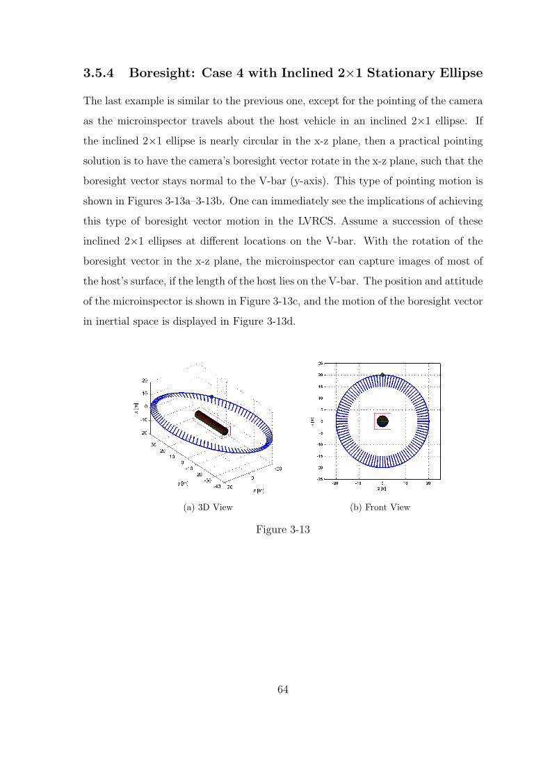
3.5.4 Boresight: Case 4 with Inclined 2×1 Stationary Ellipse

The last example is similar to the previous one, except for the pointing of the camera

as the microinspector travels about the host vehicle in an inclined 2×1 ellipse. If

the inclined 2×1 ellipse is nearly circular in the x-z plane, then a practical pointing

solution is to have the camera’s boresight vector rotate in the x-z plane, such that the

boresight vector stays normal to the V-bar (y-axis). This type of pointing motion is

shown in Figures 3-13a–3-13b. One can immediately see the implications of achieving

this type of boresight vector motion in the LVRCS. Assume a succession of these

inclined 2×1 ellipses at different locations on the V-bar. With the rotation of the

boresight vector in the x-z plane, the microinspector can capture images of most of

the host’s surface, if the length of the host lies on the V-bar. The position and attitude

of the microinspector is shown in Figure 3-13c, and the motion of the boresight vector

in inertial space is displayed in Figure 3-13d.

(a) 3D View (b) Front View

Figure 3-13

64

EarthX

Z

Geocentric

Reference

Frame+y

-y

(c) Inertial Reference Frame

−1−0.5

0−0.4−0.200.20.4

−1

−0.5

0

0.5

1

X [m]Y [m]

Z [m

]

(d) Camera’s Boresight Vector in Inertial Refer-ence Frame

Figure 3-13: Boresight Case 4 with Inclined 2×1 Stationary Ellipse: The microin-spector in an inclined 2×1 stationary ellipse about the host.

3.6 Sun Angle and Recharging Batteries

Another aspect of the microinspector that must be examined before designing the

mission is the power system. This thesis focuses specifically on a microinspector

design that is equipped with solar cells for continuous operation in the Sun and

batteries when solar energy is not available. The sun angle, φsa, is defined here as

the angle between the light ray from the Sun and the vector normal to the solar cells

on the microsatellite. Figure 3-14 gives a graphical definition. This type of hardware

setup for the microsatellite allows operation of all power consuming systems when the

sun angle is less than some specified angle, φsa,max, via the solar cells alone. During

this time, if the battery reserves are less than the maximum capacity, these batteries

can be recharged by the solar cells. φsa,max is less than or equal to 90◦, and may be

determined by the average power usage by the microsatellite. While φsa > φsa,max,

the microinspector can run off the batteries, until the sun angle is once again adequate

for solar cell usage. In summary,

• φsa > φsa,max: Batteries are discharging

• φsa < φsa,max: Batteries are charging

65

Solar Cells

Sunlight

vector

Normal vector to

solar cells

ϕsa

Figure 3-14: Sun Angle, φsa

In this thesis, “solar cell mode” is when the batteries are charging, and “battery

mode” is when the batteries are being discharged. In order to determine the proper

specifications for the microinspector’s power system, the amount of time spent in

solar cell mode and battery mode during a typical orbital maneuver needs to be

evaluated. One obvious goal in designing a mission for a microinspector with solar

cells is to stay in solar cell mode for the majority of the mission time. If the battery’s

state of charge (SOC) is below the specified minimum SOC, it will become necessary

to recharge by pointing the solar cells toward the Sun, during the mission. Since

this takes time away from the inspection part of the mission, it is desired to avoid

these recharging maneuvers, if possible. While still attaining the desired motion of

the camera boresight vector, the orientation of the microinspector that minimizes φsa

throughout the mission must be determined. For the following analysis, φsa,max is

assumed to be 90◦. Another assumption is that the solar cells are placed only on one

side of the microsatellite, as shown in Figure 3-14. The camera viewpoint is located

on one of the edges of this box shaped microinspector model.

Five different cases are discussed to illustrate the problem. The first three cases

depict an in-plane 2×1 elliptical motion by the microinspector in the LVRCS, with

different lighting and phasing conditions. The boresight vector appears to rotate at

the constant orbital rate and is initialized to point at the host’s surface, as in Figure 2-

7a. In the fourth case, the microinspector is stationary behind the host vehicle on

66

the V-bar, with the camera’s boresight vector pointing at the host. Finally, in the

fifth case, the microinspector is placed in an inclined 2×1 ellipse in the LVRCS.

The camera’s boresight vector appears to rotate at the constant orbital rate in the

LVRCS, and is always perpendicular to the V-bar, as in Section 3.5.4. The scales of

the vehicles are exaggerated in all figures, in order to present the concept.

3.6.1 Sun Angle: Case 1 with Sun Facing the Orbital Plane

of Host

In the first case, the Sun faces the orbital plane of the host and the microinspector

is placed in a 2×1 ellipse about the host vehicle. In the inertial reference frame,

the microinspector does not rotate about its axes. However, in the LVRCS, this

corresponds to constant angular rotation of the boresight vector, which allows the

microinspector to capture images of a large portion of the host’s surface, as shown in

Figure 3-15a. In order to maximize Sun exposure to the solar cells, the microinspector

can be initially oriented so that the solar cells face the Sun, as seen in Figure 3-15b.

Then, throughout the 2×1 ellipse motion, φsa = 0, permitting the vehicle to operate

solely on solar energy. This case is ideal for power usage, since the reserve batteries

are never used.

67

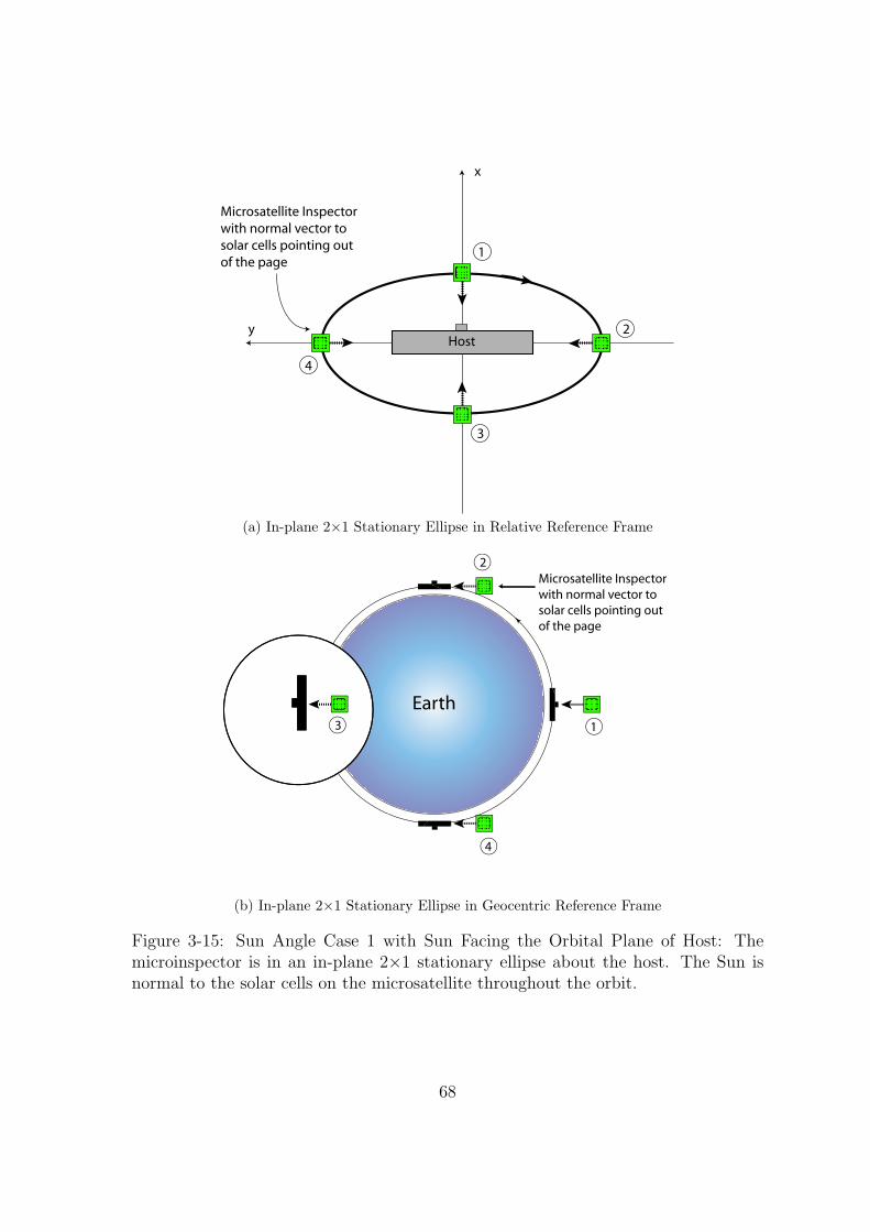
x

yHost

1

2

3

4

Microsatellite Inspector

with normal vector to

solar cells pointing out

of the page


Earthr

v

Microsatellite Inspector

with normal vector to

solar cells pointing out

of the page

1

2

3

4

(b) In-plane 2×1 Stationary Ellipse in Geocentric Reference Frame

Figure 3-15: Sun Angle Case 1 with Sun Facing the Orbital Plane of Host: Themicroinspector is in an in-plane 2×1 stationary ellipse about the host. The Sun isnormal to the solar cells on the microsatellite throughout the orbit.

68

3.6.2 Sun Angle: Case 2 with Sun in Orbital Plane of Host

In contrast, the second case presents the worst possible scenario for power consump-

tion. The Sun is in the same plane as the host’s orbital plane, and the microinspector

is again in a 2×1 ellipse about the host vehicle. When the top of the host vehicle is

normal to the Sun, the microinspector is positioned and oriented, so that the camera

has a view normal to the top of the host. In traveling ellipse terms, the in-plane phase

angle starts at 90◦. This is illustrated in Figure 3-16b. As in the first case, a large

percentage of the host’s surface may be captured with this setup. However, there is

no orientation of the microinspector that will give the proper Sun exposure to the

solar cells. Thus, the sun angle can never be less than 90◦, which signifies that the

batteries are not recharged throughout the 2×1 ellipse motion, the batteries must be

used. Upon energy depletion, the batteries must be recharged by pointing the solar

cells toward the Sun.

x

yHost

1

2

3

4Solar Cells

Solar Cells

Solar Cells

Solar Cells


Figure 3-16

69

Earth

Sunr

v

13

4

Solar Cells

2

Solar Cells

Solar Cells

Solar Cells


Figure 3-16: Sun Angle Case 2 with Sun in the Orbital Plane of Host: The microin-spector is in an in-plane 2×1 stationary ellipse about the host. When the top of thehost vehicle is normal to the Sun, the microinspector is positioned and oriented, sothat the camera has a view normal to the top of the host.


The third case is similar to the previous one in all aspects, aside from the phasing.

When the top of the host vehicle is normal to the Sun, the microinspector is positioned

at an in-plane phase angle of 45◦ in the 2×1 ellipse, and oriented so that the boresight

vector points toward the host at a 45◦ angle. If the microinspector is initially oriented

so that the sun angle is minimized, then the solar cells have Sun exposure during the

orbit, outside of Earth’s shadow, as displayed in Figure 3-17. φsa = 45◦ for nearly

two-thirds of the orbital period, so the back-up battery need only be used in Earth’s

shadow, assuming that φsa,max is greater than 45◦. Depending on the specifications of

the battery and solar cells, specific recharging maneuvers may not need to be included

in the mission. The battery may be sufficiently recharged during the solar cell mode.

This example shows the importance of phasing the relative motion appropriately, to

optimize solar cell usage.

70

x

yHost

1

2

3

4Solar Cells

Solar Cells

Solar Cells

Solar Cells


Earth

Sunr

v

13

4

Solar Cells

2

Solar Cells

Solar Cells

Solar Cells

4


Figure 3-17: Sun Angle Case 3 with Sun in the Orbital Plane of Host: The microin-spector is in an in-plane 2×1 stationary ellipse about the host. The initial in-planephase angle is 45◦ in the 2×1 ellipse and oriented so that the boresight vector ispointed toward the host at a 45◦ angle.

71

From the lighting cases presented in this section and Section 3.6.2, it can be

inferred that if the initial in-plane phase angle is 90◦, then the attitude of the mi-

croinspector can be initialized to have the solar cells always pointing at the Sun.

φsa = 0◦ when not in Earth’s shadow, during the orbit. In contrast to the case in

Section 3.6.2, the solar cells are ideally positioned; however, the host’s surface that is

in the FOV of the camera, is never illuminated and no images can be obtained with

this setup.

For the microinspector trajectory and attitude setup in this section and Sec-

tion 3.6.2, some of the limitations in the trade-off between observing the host and

charging the batteries may be mitigated if the vector normal to the solar cells is

opposite in direction to the camera’s boresight vector.


Figure 3-18 illustrates the next case. The microinspector is placed in the same orbit

as the host vehicle, but slightly behind. In the LVRCS, the microinspector appears to

be stationary on the V-bar behind the host vehicle, as shown in Figure 3-18a. In the

inertial reference frame, the microinspector is rotating at the constant orbital rate.

The camera’s boresight vector is pointed toward the edge of the host, parallel to the

V-bar. Without disturbing the position of the microinspector and boresight vector,

battery usage may be minimized by initially orienting the solar cells’ normal vector

parallel to the host vehicle’s radial vector and away from the center of the host’s

orbit. This orientation allows φsa to be less than φsa,max = 90◦ for about half the

orbital period during one orbit. Therefore, the solar cells can be used for continuous

operation for nearly half the orbital period. When φsa > φsa,max and when the host

vehicle is in the Earth’s shadow, the microinspector must switch to battery mode to

continue operating. Once again, specific recharging maneuvers may not be necessary

given the specifications of the battery and solar cells.

72

x

yHost

Solar Cells

(a) Stationary on V-bar in Relative Refer-ence Frame

Earth

Sun

Solar Cells

Solar Cells

Solar Cells

Solar Cells

(b) Stationary on V-bar in Relative Reference Frame

Figure 3-18: Sun Angle Case 4 with Sun in the Orbital Plane of Host: The microin-spector is stationary on the V-bar behind the host vehicle. The camera’s boresightvector is pointed toward the edge of the host.

73


Finally, in the last example, the microsatellite inspector is in an inclined 2×1 station-

ary ellipse about the host vehicle. The camera’s boresight vector is pointed toward

the host, normal to the surface, as in Section 3.5.4. The view down the V-bar looks

circular for this particular case. To achieve this type of relative motion, a rotational

∆v must be applied at positions ➀–➃ to spin-up the attitude to the orbital rate in

the directions shown in Figure 3-19b. The camera’s boresight vector follows the path

illustrated in Figure 3-13d. With no further attitude control maneuvers, the solar

cells are exposed to the Sun for less than a third of the orbital period. However,

upon closer inspection, this example brings a new possibility to light. There is an

extra degree of freedom about the camera’s boresight vector, which can be utilized to

acquire more Sun exposure to the solar cells. In this example, the microinspector can

be rotated 180◦ about the boresight vector at positions ➀ and ➂, as shown in Fig-

ure 3-19. These rotations result in doubling the Sun exposure time, and consequently

the time spent using the solar cells for operation. Under different lighting conditions

and given enough fuel, the mission planner may choose to actively control the ori-

entation of the microinspector about the boresight vector, in order to maximize the

Sun exposure to the solar cells. This sun angle minimizing algorithm will be referred

to as the Sun-nadir pointing scheme, for the remainder of this thesis.

74

x

Solar Cells

3 Rotate 180 ° about boresight vector

Rotate 180 ° about boresight vector1

Solar Cells

Solar Cells

Solar Cells

Solar Cells

y1

2

3

4

z

Host

x

z

x

Solar Cells

x

(a) Inclined 2×1 Stationary Ellipse in Relative Reference Frame

Figure 3-19

75

Earth

Sun12

4

3

Solar Cells after

180 ° rotation

about boresight

vector

Solar Cells after

180 ° rotation

about boresight

vector

Solar Cells

Solar Cells

(b) Inclined 2×1 Stationary Ellipse in Relative Reference Frame

Figure 3-19: Sun Angle Case 5 with Sun in the Orbital Plane of Host: The microin-spector is in an inclined 2×1 ellipse about the host vehicle. The camera’s boresightvector is pointed toward the host, normal to the surface.

3.6.6 Recharging

In reality, φsa,max will be much less than 90◦, due to the average power needed to

continue running all systems on board the microinspector. Additionally, the battery

reserves will not be completely depleted before conducting recharging maneuvers. For

instance, assume that the maximum power attained from the solar cells is 25W , which

corresponds to a sun angle of 0◦. The solar array is assumed to have cosine losses;

therefore, at sun angles less than 90◦, the amount of power that can be obtained from

the solar cells is approximately given by Eqn 3.34.

Power from solar cells (W ) = 25 cos(φsa), for 0◦ ≤ φsa ≤ 90◦ (3.34)

Let the peak capacity of the battery be 45W ·hr. If the average power used for

operation of the microinspector is 14W , then continuous usage of the battery will

completely drain it in about 3.2hrs. Recharging the battery from this drained state

takes about 4hrs at a 0◦ sun angle. At sun angles greater than 56◦, the solar cells

produce less than 14W , so the microinspector must switch to battery mode. Thus,

76

φsa,max is defined to be 56◦.

3.7 Mission Assessment through Figures of Merit

Rating the successfulness of an inspection mission by a microinspector depends greatly

on the host spacecraft and the type of inspection that is desired. For example, a mi-

crosatellite inspector may be used to observe the solar sails unfurl from a sailcraft.

This particular mission would probably require the microinspector to be placed afar

and point at the host vehicle, in order to capture the entirety of the solar sail deploy-

ment. Another use for a microinspector would be to take images of the surface of a

manned space vehicle for damage. Unlike the sailcraft mission, the microinspector

would need to maneuver about the host vehicle to capture images of the complete

surface. The resolution of the images would be considered an important measure of

success for this mission. This section presents some figures of merit that would be

useful to rate and design an inspection mission. Most likely, no one figure of merit

will be adequate in rating the quality of a mission. The mission designer must apply

an appropriate weighting factor to each of several possible figures of merit.

3.7.1 Fuel Expenditure

Fuel expenditure is a figure of merit that is key in rating and designing any microsatel-

lite mission. Because of the limited amount of fuel on board a typical microsatellite,

trajectory design for a mission that minimizes fuel usage is highly desirable. Fuel ex-

penditure can dramatically reduce the usable mission lifetime of the microinspector

when a complex re-docking and re-fueling option is not available. If the actuators

for attitude control are the same thrusters used for translational motion, then fuel

minimization becomes even more critical. This thesis assumes that the microinspec-

tor has no momentum exchange devices on board for attitude control, and that the

thrusters are used for both translational and rotational maneuvers.

77

3.7.2 Host Surface Coverage

For visual inspection missions that survey the total surface area of the host vehicle,

a figure of merit is needed to ensure that the microinspector captures images of

the entire surface. A simple method is to divide the surface of the host vehicle

into segments. When the center point of a segment is in the field of view (FOV)

of the camera and the segment is illuminated by sunlight, the complete segment is

assumed to be viewed, in this thesis. The smaller the segments are made, the more

accurate this assumption. Thus, throughout the course of the mission, the sections

of the host that are viewed can be determined by this figure of merit. Figure 3-20

illustrates the points on the surface of the host vehicle model. A vector normal to

the surface at each point is drawn in the figure. Figure 3-21 displays the surface

area of the cylindrical host model. Each segment is represented by a number. If all

the segments are viewed by the microinspector, then this figure of merit affirms that

the microinspector successfully captures images of the total surface. The top row

in Figure 3-21 represents the top of the host surface in the LVRCS frame when the

length is along the V-bar. The fifth row represents the bottom of the host surface.

−20

−10

0

10

20−10

0

10

−15

−10

−5

0

5

10

15

z [m]y [m]

x [m

]

Figure 3-20: Points on Surface of Host Spacecraft

78

Figure 3-21: Surface Grid Labeling of Host Vehicle Segments

To determine whether or not a point on the surface of the host appears in an

image taken by the camera, at least two conditions must be fulfilled. First, the point

must be within the conical FOV of the camera. Second, the view must be visable to

the camera with no obstruction. Figure 3-22 provides an illustration of the vectors

and angles used in the calculations to determine if the conditions are met.

rlos

rc,pt

rn θ

aov

Figure 3-22: Host Surface and Camera Vectors and Angles

With θaov as the angle of view of the camera, rlos as the boresight unit vector

from the camera, rc,pt as the position vector from the camera to the point on the

surface, and rn as the normal vector to the point on the surface, the calculations to

demonstrate that the two conditions are met are as follows:

1. Point is contained in FOV: cos−1(

rlos·rc,pt

|rlos||rc,pt|

)

≤ θaov

2

2. Point is viewable by the camera: rc,pt · rn > 0

79

If both these conditions are met, then the point on the surface of the host is said to

be visible to the camera.

3.7.3 Frequency of Host Surface Coverage

Another figure of merit that is directly correlated with viewing points on the host’s

surface is the frequency or total time that a point is viewed. In a typical mission, it

is foreseen that some sections of the host’s surface may be captured more often than

others. A figure of merit relating the frequency of the viewed points would provide

knowledge on which sections the microinspector has more opportunities to view and

image. In mission simulations, the frequency can be determined by summing the

number of times the point is in the FOV of the camera per time step.

3.7.4 Angles of Host Surface Coverage

The inspection mission may require the microinspector to take images of the host’s

surface at different angles. The angle variety provided by the assorted images gives

perspective on any possible damage to the surface. If all the images are taken normal

to the surface, an object that is loose or raised may not be apparent. For a general

overview of the host’s surface, it is desirable to acquire a multifaceted portrait of

the vehicle through the images taken by the microinspector. A figure of merit that

depicts the variety of angle views of the host surface would rate how close the mission

is to achieving this goal.

3.7.5 Lighting

Some problems associated with lighting from the Sun were discussed earlier in Sec-

tion 2.4. Even if the surface of the host vehicle is in the FOV of the camera, without

proper lighting, the camera will not be able to take observable images. When avail-

able, utilizing sunlight to take photographs is preferable to using a flash illuminator,

which would otherwise unnecessarily drain the battery. Additionally, the angle of

incidence of the sunlight on the surface of the host must be sufficient.

80

A figure of merit which falls under the category of lighting is the availability of

sunlight for image capturing. The three conditions that must be met to determine

this are:

1. Sunlight illuminates the surface being viewed

2. The point is not in the shadow of the host itself

3. The point is not in the shadow of the Earth

Figure 3-23 provides an illustration of the vectors used in the calculation to de-

termine if conditions 1 and 2 are met.

rn

rs,LVRCS

Figure 3-23: Host Surface Normal Vector and Sun Vector

With rs,LV RCS as the Sun vector in the LVRCS, and all other variables as in

Section 3.7.2, the calculation to demonstrate that the point is illuminated by the Sun

and not in the shadow of the host is as follows:

rs,LV RCS · rn > 0

Figure 3-24 illustrates Earth’s shadow and the position of the point on the surface

being imaged. Re represents the mean radius of the Earth.

81

To Sun

Earth’s Shadow

Re

rpt

ûs

Figure 3-24: Geometry of Earth’s Shadow

Based on the variables defined in this figure, the point is in the shadow of the

Earth if:

• rpt · us < 0

• |rpt · us| < Re

3.7.6 Image Resolution

The images taken by the camera on board the microinspector vehicle are beneficial

only if the quality is acceptable. Consequently, the resolution of the image is a crucial

figure of merit to evaluate the inspection mission. The image resolution for a point

on the host’s surface can be calculated by:

Resolution = rc,pt tan

(

θaov

N

)

(3.35)

rc,pt is the distance from the camera to the point on the host’s surface, θaov is the

camera’s angle of view, and N is the number of pixels in the array.

3.7.7 Pixel Smear

The requirement on the minimum pixel smear directly impacts the maximum relative

velocity of the microinspector. In Section 2.2, a requirement of less than one pixel

82

was given. This translates to keeping the relative velocity below a certain threshold

during the inspection, such that within an exposure time, an image does not spread

over more than one pixel.

To achieve this requirement, the maximum tangential relative velocity of the mi-

croinspector for a camera exposure time of tet is given by:

vmax =rc,pt tan

(

θaov

N

)

tet(3.36)

where rc,pt, θaov, and N are as before in Section 3.7.6.

3.7.8 Battery Reserve

The amount of battery power available at any given time is an important figure of

merit. If the battery reserves are drained below a certain limit, the microinspector

will need to stop its current task and point the solar cells towards the Sun to recharge.

This also impacts fuel expenditure, as well as any time constraints. At any given time,

the battery reserves can be roughly determined by:

Battery Reserves (W ·hr) =

B0 + 25

t∫

t0

[cos(φsa) − cos(φsa,max)] dt (3.37)

where B0 is the battery reserve at t0.

83


84

Chapter 4

Design Description

The strategies presented in Chapter 3 allow a straightforward mission design for a

microsatellite inspector in a planet orbiting environment. The idea of utilizing nat-

ural dynamics in designing the trajectory was found to use extremely minimal fuel.

In addition, the CW solution provides an easy method for calculating the positions,

velocities, and accelerations for natural trajectories. Thus, in this chapter, a list of

some of the natural relative trajectories that may be advantageously employed in a

visual inspection mission is presented. These trajectories form a toolset that a mis-

sion planner can use in building an inspection mission. Methods and fuel usage for

transferring from one type of trajectory to another is discussed. Methods used to esti-

mate fuel usage for rotational motion and station-keeping are also examined. Finally,

a baseline mission description for a microinspector utilizing the design strategies and

the trajectory toolset is presented.

4.1 Toolset

This section recounts some of the natural relative motion presented thus far, as well as

introducing a new set of trajectories that may be exploited in designing an inspection

mission. An analysis of each trajectory is conducted on the basis of fuel usage,

application to imaging, and time span, all in the LVRCS. The velocity magnitude of

each of the following trajectories is much less than the maximum ∆v that would be

85

available on a microsatellite inspector.

4.1.1 Stationary on V-bar

One option for inspection is to place the microinspector behind or in front of the

host, along the V-bar, as shown in Figure 4-1. Examples of this type of trajectory

were already given in Figures 2-8, 3-11, and 3-18. In the LVRCS, the camera can be

directed to point toward the host. If the host is equipped with solar arrays or solar

sails, the microinspector can capture the deployment phase while in this stationary

position, relative to the host. Another application would involve the cooperation of

the host vehicle. The host spacecraft can rotate about different axes in the LVRCS

allowing the microinspector to take images of the host until complete coverage is

achieved. This stationary position may also be utilized as an intermediary point

before embarking on the remainder of the inspection mission. In terms of the traveling

ellipse parameters from Section 3.1.2, Y0 defines where the microinspector is located

on the V-bar relative to the host. All other parameters are set to a value of zero.

Once the microinspector is put on the V-bar near the host vehicle with zero relative

velocity, the microinspector stays at the position indefinitely, with fuel being used

only for orbit maintenance.

Figure 4-1: Stationary on V-bar

86

4.1.2 Out-of-plane Oscillation across the V-bar

The microinspector can also be made to oscillate out-of-plane, while positioned on

the V-bar. The out-of-plane magnitude is defined by the traveling ellipse parameter,

c. As in Section 4.1.1, the position on the V-bar is designated by the value of Y0.

Figure 4-2 portrays an out-of-plane motion, with c = 10m, which requires a velocity

burn of ∆v = 0.00996m/s, from a zero-velocity state on the V-bar. An out-of-plane

motion with a magnitude of c = 20m requires ∆v = 0.01992m/s. The larger the

magnitude, the greater the initial velocity needs to be to insert the microinspector

into this oscillatory motion. If the length of the host spacecraft lies out-of-plane as

in the figure, the advantage of the out-of-plane natural motion becomes apparent.

Placed in this oscillatory motion, the microinspector can take images of the entire

length of the host vehicle.

Figure 4-2: Out-of-plane on V-bar

4.1.3 In-plane 2×1 Ellipse

The 2×1 elliptical motion, also known to the GN&C community as a football orbit, was

introduced in the previous chapters. The in-plane 2×1 ellipse is a stationary relative

closed orbit, which was illustrated in Figures 2-7 and 3-10–3-12. The position of an

in-plane 2×1 ellipse along the V-bar may vary depending on the mission requirements.

87

The cases presented next are considered to be basic to the trajectory toolset for an

inspection mission.

Center at Origin

An in-plane 2×1 ellipse presents a stable and fuel-minimizing method of traveling

about the host vehicle. The attitude of the microinspector can be regulated so that

the camera’s boresight vector is fixed in the inertial reference frame, as discussed in

the example in Section 3.5.1. Once the microinspector is inserted into this stationary

ellipse, no further fuel is needed to continue the motion about the host vehicle. Hence,

the in-plane 2×1 ellipse is not only an excellent choice for an inspection trajectory, it

is also an ideal trajectory to be put into during intervals of non-imaging.

Figure 4-3 illustrates an in-plane 2×1 ellipse, in which b = 20m and Y0 = 0m. All

other traveling ellipse parameters are set to zero. The velocity burn for insertion is

∆v = 0.022m/s, from a zero-velocity state at 40 or -40m on the V-bar. The velocity

magnitude during a 2×1 ellipse is minimum where the ellipse intersects the V-bar

(y-axis) and maximum where it intersects the R-bar (x-axis). An ellipse that is twice

the size of the one in Figure 4-3 would require double the ∆v for insertion. The time

for one revolution about the host vehicle is the same as the orbital period of the host.

Figure 4-3: In-plane 2×1 Ellipse: Center at Origin

88

Off-center Ellipse

The center of the in-plane 2×1 ellipse can be offset along the V-bar as shown in

Figure 4-4. This type of trajectory has advantages similar to the previous case. It

may be utilized for inspection of the host spacecraft or for placing the microinspector

in a stable relative motion during intervals of non-imaging. The velocity magnitude

needed to insert the microinspector into the trajectory is ∆v = 0.012m/s.

Figure 4-4: In-plane 2×1 Ellipse: Center Not at Origin

Intersecting Ellipse

The center of the in-plane 2×1 ellipse can be offset along the V-bar as shown in

Figure 4-5, such that the trajectory intersects with the host vehicle. Although this

type of trajectory is not suited for inspection purposes due to the danger of collision,

using a portion of the trajectory is certainly a valid method for initially deploying

the microinspector. One can envision the microinspector leaving the host, traveling

along this trajectory, and stopping once it reaches the V-bar. In the figure, the

dot represents the initial position of the microinspector attached to the host. Also,

the complete trajectory — when the microinspector is not stopped at the V-bar

— is shown. The velocity magnitude needed to insert the microinspector into the

trajectory is ∆v = 0.012m/s.

89

Figure 4-5: In-plane 2×1 Ellipse: Intersecting Ellipse

4.1.4 Inclined 2×1 Ellipse

Examples that involved an inclined 2×1 ellipse were illustrated in Figures 2-9, 3-3,

3-12–3-13, and 3-19. Similar to the in-plane 2×1 ellipse case, this type of trajectory

allows for a stable and fuel minimal method of orbiting about or near the host vehicle.

The form of the trajectory is still a 2×1 ellipse in-plane. The inclined portion of the

trajectory comes directly from the addition of the out-of-plane oscillatory motion to

the in-plane 2×1 ellipse. A variety of inclined 2×1 ellipses may be formed specific

to the inspection mission, by varying the values for b, c, Y0, and ψ − φ. X0 must be

zero for the relative orbit to stay stationary. In this study, two distinct forms of the

inclined 2×1 ellipse are presented for their natural benefits in visual inspection.

Circular in x-z Plane

Figure 4-6 displays an inclined (about the R-bar) 2×1 ellipse that is circular when

viewed along the V-bar, in the x-z plane of the LVRCS. To obtain such a relative orbit,

the value for b and c must be equal. Additionally, ψ − φ = 90◦. For a host vehicle

with its length along the V-bar, this type of trajectory permits the microinspector

to get closer to the surface and take images with better resolution, with minimal

risk of collision. The size of the inclined ellipse can be made much smaller than an

in-plane ellipse, in part because of the out-of-plane factor and also due to the ellipse

90

intersecting the R-bar instead of the V-bar. In effect, the value for the semiminor

axis, b, has more flexibility. The camera’s boresight vector can be initiated to rotate

in the plane of the ellipse, as in Figure 3-12. Another practical option is to direct

the attitude of the microinspector, so that the camera’s boresight vector is normal

to the V-bar, as in Figure 3-13. The velocity magnitude of this inclined 2×1 ellipse

at φ = 0◦ and φ = 180◦ is the same as its in-plane counterpart: v = 0.011m/s. At

φ = 90◦ and φ = 270◦, the velocity magnitude of the microinspector is v = 0.025m/s.

Again, the period of the inclined 2×1 ellipse is equal to the orbital period of the host.

(a) 3D (b) Front View (x-z View)

Figure 4-6: Inclined 2×1 Ellipse: Circular in x-z Plane

Because the trajectory does not intersect the V-bar, even if some drift occurs along

the V-bar due to differential perturbing accelerations, there is no chance of collision.

Thus, this motion is safe in terms of collision and easy to maintain.

Circular in Orbital Plane

The x-y plane view of an inclined 2×1 ellipse always has the 2×1 form. But in the

orbital plane of the relative trajectory, the shape can be varied dramatically. Figure 4-

7 illustrates one particular trajectory that can be achieved. The inclined (about the

V-bar) ellipse is such that the motion is circular about the center of the relative orbit,

and the trajectory intersects the V-bar. For a given value of b, setting c = ±b√

3

91

and ψ − φ = 0◦ gives the circular form in the relative orbital plane. The camera’s

boresight vector can be controlled to rotate in this plane, while pointing toward the

center of the circular relative motion. The microinspector is equidistant from this

center throughout its motion, which may be beneficial to some inspection missions.

These circular relative orbits, however, are always inclined 60◦ from the in-plane,

possibly restricting their use. Since the orbit intersects with the V-bar, the danger of

collision is also increased if the microinspector is close to the host.

Figure 4-7: Inclined 2×1 Ellipse: Circular in Orbital Plane

4.1.5 Horizontal Above/Below

The CW solution shows that the microinspector can be made to move in a relative

straight line above or below the host in-plane. This type of motion can be used to

view the top or bottom of the host vehicle at a constant distance from the V-bar,

if the host is not rotating in the LVRCS. Also, a nonzero value for c will result in

an out-of-plane sinusoidal motion. Figure 4-8 shows what this type of motion looks

like, relative to the host vehicle, which maintains a LVLH attitude. The velocity

magnitude needed to set the microinspector to traverse in a straight line depends

on the position deviation along the R-bar (x-axis), and is given by Eqn 4.1. The

velocity is applied parallel to the V-bar, which makes the microinspector appear to

92

move above or below the host vehicle depending on the sign of the radial deviation

from the host.

v = −3

2x0ω (4.1)

Figure 4-8: Horizontal Motion Above/Below Host Vehicle

4.1.6 In-plane Traveling Ellipse

The traveling ellipse was first introduced in Section 3.1.2, Figure 3-4. This relative

motion occurs when the center of the stationary ellipse along the radial vector is

not located on the V-bar of the host spacecraft. In traveling ellipse parameters, the

value of X0 is nonzero. By shifting the center of the original 2×1 ellipse up or down

along the radial axis, the ellipse appears to move backwards or forwards, respectively.

In general, a drifting ellipse in-plane is usually an undesirable phenomenon due to

possible collision with the host.

Inserting the microinspector into an in-plane traveling ellipse trajectory is an

effective method of disposing the vehicle once the inspection mission is completed.

Figure 4-9 illustrates two instances of the microinspector leaving its initial stationary

position on the V-bar via a traveling ellipse. The fuel needed to enter such a trajectory

is extremely small compared to the total fuel on board a microinspector.

93

Figure 4-9: In-plane Traveling Ellipse

4.1.7 Spiral Orbit

The spiral orbit is essentially an inclined traveling ellipse. Given the right set of

conditions, the microinspector can be made to drift along the V-bar in a spiraling

loop with no further use of fuel, as shown in Figure 4-10. In this particular figure,

the host is in a circular orbit about the Earth at an altitude of 500 km. The initial

velocity magnitude of the spiral orbit is v = 0.011m/s from a zero velocity state. The

spiral orbit can be initiated from a corresponding inclined 2×1 ellipse. By applying

a ∆v parallel to the V-bar, the microsatellite can be made to spiral forwards or

backwards. The effect of applying ∆v parallel to the V-bar is elaborated further in

Appendix B. The camera’s boresight vector can point toward the host’s surface, much

like in Section 4.1.4, throughout the orbit. This is an excellent method of capturing

images of the host’s surface, while using very little fuel. For host vehicles, whose

length is along the V-bar, this method can be used to inspect most of the host’s

surface. Similar to the first case (circular in x-z plane) in Section 4.1.3, there is no

chance of collision as the microinspector travels along the spiral trajectory. Thus, the

motion is safe in the presence of disturbing differential accelerations. While traveling

forwards or backwards, there is no possibility of collision. As seen in Figure 4-10b,

the spiral trajectory forms a tunnel around the host vehicle. Each loop of the spiral

orbit is approximately one orbital period. The values for b, c, X0 and φ − ψ, which

determine the size and shape of the spiral, will depend on the camera specifications

and image requirements.

94

(a) 3D

(b) Front View

Figure 4-10: Spiral Orbit

95

4.1.8 Tear-drop Orbit

This trajectory is so named because of its tear-drop shape. The trajectory is actually

just a segment of one revolution of the traveling ellipse; however, the ease in which the

tear-drop form can be kept with periodic maintenance makes it a useful trajectory

to include in the toolset. The time to traverse a tear-drop orbit is less than one

orbital period, since it is a section of the traveling ellipse. Thus for missions that

are constrained in time, utilizing tear-drop orbits may be a practical choice, with the

trade-off being periodic fuel expenditure.

Tear-drop About Host

The shape and the position of the tear-drop orbit may be chosen to encircle the host

vehicle, as illustrated in Figure 4-11. The motion of the microinspector is purely

in-plane. Without the ∆v burn at the point of intersection of this tear-drop orbit,

the microinspector will follow the path of a traveling ellipse. The “period” or ∆ttd of

this tear-drop orbit is about 95% of the orbital period of the host. ∆v ∼= 0.005m/s,

which is applied in the negative x-direction every ∆ttd. In Section 3.5.1, the camera’s

boresight vector was rotated in the LVRCS to capture images of the host vehicle.

Since ∆ttd is less than the orbital period, the boresight vector needs to be rotated

at a constant angular rate of 2π∆ttd

rad/s. The deviation of the ellipse’s center is

positive along the radial axis in Figure 4-11. If the deviation is negative, then the

microinspector would move along a traveling ellipse path in the opposite direction.

The ∆v burn would then have to be applied in the positive x-direction to achieve a

tear-drop orbit about the host vehicle.

96

Figure 4-11: Tear-drop Orbit About Host (In-plane)

The tear-drop orbit may also be designed to have an out-of-plane component.

Because the out-of-plane motion is sinusoidal with a period equaling the orbital period

of the host vehicle and ∆ttd is less than the orbital period, the out-of-plane location

of ∆v will vary from burn to burn. Over time, the tear-drop orbits form a set that

stays within a band defined by the out-of-plane traveling ellipse component, c. The

motion is akin to a lissajous figure in three dimensions. Figure 4-12 displays the same

in-plane tear-drop shape from Figure 4-11, but with an out-of-plane component of

c = 3m. The ∆v burns are equivalent in magnitude and direction.

Figure 4-12: Tear-drop Orbit About Host (3D)

97

Tear-drop Near Host

The tear-drop orbit can also be formed near the host vehicle as in Figure 4-13. This

type of trajectory can be utilized to take an image of a particular point on the host

vehicle, without resorting to station-keeping. Station-keeping at a position above or

below the host would require much more fuel consumption, than this tear-drop orbit.

Since only one snapshot of the point on the surface is needed to determine if the vehicle

has been damaged, the tear-drop trajectory, such as the one in Figure 4-13 will suffice.

It is not necessary to continue traveling about the tear-drop shape, and thus extra

burns are not needed. Nevertheless, if it is desired to have the microinspector travel

about the tear-drop orbit as in Section 4.1.8, then similarly a ∆v burn is required each

time the microinspector reaches the point of intersection. The smaller the tear-drop

orbit becomes, the closer the total ∆v is to the fuel for station-keeping at the limiting

point. This is one method for mechanizing the station-keeping method.

Figure 4-13: Tear-drop Orbit Near Host

Notice that the tear-drop shape can be eliminated altogether, to form a dip in

place. Figure 4-14 illustrates this trajectory.

98

Figure 4-14: Dip Near Host

4.2 Trajectory Transfer and Location of Transla-

tional ∆v Burns

Before the natural motions presented in the toolset from Section 4.1 can be utilized

to piece together a mission, it is necessary to list the possible transfers from one type

of motion to another. Figure 4-15 portrays a flowchart of the natural motions from

the toolset and the transfers between them. Many of the trajectories listed in the

toolset are subsets of the inclined 2×1 ellipse and the inclined traveling ellipse. Thus,

in the flowchart, the trajectories that proceed from these categories are shown in the

dashed boxes. All of the trajectories in the flowchart are natural motion, except for

the tear-drop orbits, which lead to station-keeping.

99

Host

In-plane 2×1

Ellipse (off-center)

Stationary on V-bar

In-plane 2×1 Ellipse

Pure Out-of-plane

Inclined 2×1 Ellipse

Inclined 2×1 Ellipse :

Circul ar in the x-z

Plane

Inclined 2×1 Ellipse :

Circul ar in Orbital

Plane

Horizontal

In-plane Traveling Ellipse

Spiral : Inclined

Traveling Ellipse

Tear-drop Near Host In-plane Tear-drop

Out-of-plane Tear-

drop

r0, v

0

Figu

re4-15:

Tran

sferTra

jectoryFlow

chart

ofToolset

100

There are a variety of methods of computing the transfer trajectories to maneuver

from one natural relative motion to another. The forced motion method discussed in

Section 3.4 can be employed in this case to insert the microinspector into the desired

natural motion. However, this method is expensive in terms of fuel usage compared

to the use of natural dynamics. Hence, the transfer trajectories for the simulations

in this thesis will be computed using the natural relative dynamics described by the

CW solution. This section presents a description of several of the transfer trajectory

computations. Based on these computations, a set of positions, impulse velocities,

and times, which describe the natural motions and the transfers, are compiled into an

input array that is used by the mission simulation. Figure 4-16 illustrates the general

legend for the graphics in this section.

Initial Position

Initial Trajectory

Transfer Trajectory

Final Trajectory

Final Position

Figure 4-16: Legend for Transfer Trajectory Graphics

4.2.1 V-bar =⇒ V-bar

Table 4.1 describes the variables that are used to compute the transfer trajectory

between two positions on the V-bar. The initial relative velocity at ri is assumed to

be zero.

101

Table 4.1: V-bar =⇒ V-bar: Computational Variables

Variable Description

ri Initial position vector (on V-bar)ti Time at ri

rf Desired position vector (on V-bar)

ω Orbital rate of hostd Differential acceleration vectorbox Dimensions of box constraint

1. If ri = rf , then no transfer trajectory is needed.

2. If ri 6= rf , then the transfer trajectory can be computed using the traveling

ellipse formulation of the CW solution. The trajectory is a half-segment of an

in-plane 2×1 ellipse that connects the two positions. This in-plane 2×1 ellipse

is determined by the following traveling ellipse parameters:

b =|ri − rf |

4(4.2)

Y0 =ri + rf

2(4.3)

The value for the in-plane phase angle, φ, is either 0◦ or 180◦, depending on the

initial and final positions. All other traveling ellipse parameters for the ellipse

are zero. With these parameters, the ∆v to start the transfer trajectory can

be computed by Eqn 3.9. The desired position on the V-bar is reached after

half the orbital period, at which point an equivalent ∆v is applied to stop the

elliptical motion. Figure 4-17 illustrates this type of transfer trajectory. The

circle represents the initial position and the square designates the final desired

position on the V-bar.

102

(a) 3D View

(b) Side View (in-plane)

Figure 4-17: V-bar ⇐⇒ V-bar

103

3. If the transfer trajectory from 2 violates the avoidance constraints, alternative

measures need to be taken. The microinspector can be sent to an intermediary

position(s) on the V-bar, where the constraints are not violated traveling to

this position from the initial position. Additionally, the trajectory from the last

intermediary position to the desired position must also observe the avoidance

constraints. One way of calculating the intermediary position(s) is by using

the dimensions of the constraints. Based on the constraint dimensions, two

points can be chosen to form an elliptical transfer trajectory that stays outside

the keep-out zone. Section 3.2 explained how to determine values for b and

Y0 given two points on the 2×1 ellipse. The transfer trajectory to go from

the initial position to this constraint-avoiding 2×1 ellipse can be calculated

according to Eqns 4.2–4.3 from before. Likewise, the transfer trajectory from

this intermediary ellipse to the final desired position on the V-bar can also be

determined. The ∆v’s for each segment of the total transfer trajectory can

be determined from Eqn 3.9. A transfer trajectory that is computed with the

avoidance constraints incorporated is shown in Figure 4-18.

(a) 3D View

Figure 4-18

104


Figure 4-18: V-bar ⇐⇒ V-bar with Avoidance Constraint

4.2.2 V-bar ⇐⇒ 2×1 Ellipse

Tables 4.2–4.3 describe the variables that are used to compute the transfer trajectory

between a position on the V-bar and a 2×1 ellipse. The relative velocity at the

position on the V-bar is assumed to be zero.

Table 4.2: V-bar =⇒ 2×1 Ellipse: Computational Variables


ri Initial position vector (on V-bar)ti Time at ri

b Semiminor axis of desired 2×1 ellipsec Out-of-plane component of desired 2×1 ellipseY0 Center of desired 2×1 ellipse on y-axisθ ψ − φ for desired 2×1 ellipse


105

Table 4.3: 2×1 Ellipse =⇒ V-bar: Computational Variables


ri Initial position on 2×1 ellipsevi Initial velocity on 2×1 ellipseti Time at ri



1. To traverse from a position on the V-bar to a 2×1 ellipse, first the microin-

spector is inserted into the in-plane 2×1 ellipse, corresponding to the desired

2×1 ellipse. This in-plane 2×1 ellipse has the same traveling ellipse values as

the desired 2×1 ellipse, except c = 0. Obviously, if the desired 2×1 ellipse is

an in-plane trajectory, then the two elliptical trajectories are equivalent. The

method explained in Section 4.2.1 can be utilized to send the microinspector to

φ = 0◦ or φ = 180◦ of the in-plane 2×1 ellipse, which is located on the V-bar.

Once that position on the V-bar is reached, an appropriate ∆v can be applied

to direct the microinspector into the in-plane 2×1 ellipse. If the desired 2×1

ellipse is inclined, then at the location where the in-plane 2×1 ellipse and the

inclined 2×1 ellipse intersect, another ∆v in the out-of-plane direction can be

fired to insert the microinspector into the desired 2×1 ellipse. The ∆v’s are

calculated directly from Eqn 3.9. Figure 4-19 illustrates an example of this

transfer and the direction of the impulse velocities for this particular case.

106

(a) 3D View


Figure 4-19: V-bar ⇐⇒ 2×1 Ellipse

107

Because natural relative motion is used to design the transfer trajectories, it is

ensured that fuel is conserved. Notice that the transfer trajectory requires a

total of three ∆v burns. The first impulse velocity, ∆v1, is applied to transfer

from the initial position on the V-bar to the position designated by φ2 = 180◦

of the in-plane 2×1 ellipse, which has the same b and Y0 as the desired inclined

2×1 ellipse. Calling this corresponding in-plane 2×1 ellipse, E2, it is noted

that this trajectory intersects with the desired inclined 2×1 ellipse, E3. r2, the

position at φ2 = 180◦, can be computed simply by setting t = 0, φ2 = 180◦,

b and Y0 values to be the same as for the desired 2×1 ellipse, and all other

traveling ellipse parameters to zero in Eqn 3.8. The equation is then given by:

r2 =

b sin(φ2)

Y0 + 2b cos(φ2)

0

(4.4)

The traveling ellipse parameters, b1 and Y01 that describe the in-plane 2×1

ellipse that connects ri and r2 can be computed using Eqn 4.2–4.3. Let this

connecting in-plane 2×1 ellipse be denoted by E1. At ri, the phase angle on E1

is φ1 = 0◦. Then, ∆v1 can be computed as follows:

∆v1 =

b1ω cos(ωti + φ1)

2b1ω sin(ωti + φ1)

0

(4.5)

∆v2 is applied at r2 to insert the microinspector into E2. To determine the

second impulse velocity, the velocity at r2 on E1, v2p, and the desired velocity

on E2, v2a, must be known. ∆v2 is applied after the microinspector has traveled

half-way through the previous in-plane 2×1 ellipse at t2 = ti + P/2. Thus, v2p

can be calculated by Eqn 4.6.

108

v2p =

b1ω cos(ωt2 + φ1)

2b1ω sin(ωt2 + φ1)

0

(4.6)

At r2, the desired velocity, v2a, can be calculated by setting t = 0 and φ2 = 180◦

for E2. Eqn 4.7 shows the exact formula.

v2a =

bω cos(φ2)

2bω sin(φ2)

0

(4.7)

The second impulse velocity is then given by:

∆v2 = v2a − v2p (4.8)

Finally, the third impulse velocity is applied at the first location where E2 and

E3 intersect, denoted by r3. This position is located at either φ3 = 2π − θ or

φ3 = π−θ on E3. For the example in Figure 4-19, the value for φ3 is the former.

The calculation for r3 is given by:

r3 =

b sin(φ3)

Y0 + 2b cos(φ3)

0

(4.9)

The time for the microinspector to travel from r2 to r3 can be calculated by:

∆t2−3 =φ3 − φ2

ω(4.10)

Then, the time at which ∆v3 is applied is t3 = t2 + ∆t2−3. To compute ∆v3,

the velocity at r3 on E2, v3p, and the desired velocity on E3, v2a, must be

determined. The out-of-plane phase angle at r3 for E3 is defined as ψ3 = φ3 +θ.

v3p and v2a can be calculated by Eqn 4.11 and Eqn 4.12, respectively.

109

v3p =

bω cos(ω∆t2−3 + φ2)

2bω sin(ω∆t2−3 + φ2)

0

(4.11)

v3a =

bω cos(φ3)

2bω sin(φ3)

cω cos(ψ3)

(4.12)

The third and final impulse velocity is then given by:

∆v3 = v3a − v3p (4.13)

2. If the avoidance constraints are violated for the transfer maneuver described in

1, an intermediary position on the V-bar may be employed, as in Section 4.2.1.

From this position, the microinspector can be inserted into the desired 2×1 el-

lipse, where the path intersects with the in-plane. This transfer takes the path

of an in-plane 2×1 ellipse that connects the position on the V-bar to the inter-

secting point. The intermediary position is chosen such that the microinspector

stays outside the keep-out zone designated by the avoidance constraints. Fig-

ure 4-20 shows a case where the transfer trajectory is computed to stay outside

of the avoidance constraints. All ∆v burns can be calculated from Eqn 3.9.

110

(a) 3D


Figure 4-20: V-bar ⇐⇒ 2×1 Ellipse with Avoidance Constraints

111

The method for computing the transfer trajectories from a 2×1 ellipse to a desired

position on the V-bar is just the reverse of the methods outlined in 1 and 2.

4.2.3 V-bar ⇐⇒ r, v

Tables 4.4–4.5 describe the variables that are used to compute the transfer trajectory

between a position on the V-bar and a position outside the avoidance constraints

with some velocity. The relative velocity at the position on the V-bar is assumed to

be zero.

Table 4.4: 2×1 Ellipse =⇒ r, v: Computational Variables


ri Initial position on 2×1 ellipseti Time at ri

rf Desired position vector (on V-bar)vf Velocity vector at rf


Table 4.5: r, v =⇒ V-bar: Computational Variables





1. Utilizing the natural 2×1 ellipse trajectory to transfer from a position on the V-

bar to some position with a desired velocity simplifies the computations greatly.

First, the microinspector is sent to an intermediary position on the V-bar, using

the method described in Section 4.2.1. This intermediary position is computed

112

such that the microinspector travels for a fourth of the orbital period on the

2×1 ellipse connecting it and the final desired position, without violating the

avoidance constraints. Therefore, if the desired z component of rf is given by zd,

the traveling ellipse out-of-plane component, c, of this connecting 2×1 ellipse

is exactly zd. Once the final position is reached, a ∆v is applied to achieve

the desired velocity at that position. Figure 4-21 illustrates an example of this

transfer trajectory method. This method works as long as the final position is

not located in the y-z plane intersecting the origin. Also, close to this plane,

the fuel expenditure for the transfer trajectory also becomes quite large.

(a) 3D

Figure 4-21

113


Figure 4-21: V-bar ⇐⇒ r, v

2. When the final position is located on or near the y-z plane that intersects the

origin, another method can be used to design the transfer trajectory. A 2×1

ellipse that intersects the desired position is determined. Then, the transfer

trajectory is based on the method described in Section 4.2.2. At the desired

position, a ∆v burn is applied to achieve vf .

114

(a) 3D


(c) Front View

Figure 4-22: V-bar ⇐⇒ r, v via Inclined 2×1 Ellipse

115

The trajectory design method for the reverse transfer is simply the reverse of 1 or

2.

4.2.4 2×1 Ellipse =⇒ 2×1 Ellipse

Table 4.6 outlines the variables needed for designing and computing the transfer

trajectory from a 2×1 ellipse to another 2×1 ellipse.

Table 4.6: 2×1 Ellipse =⇒ 2×1 Ellipse: Computational Variables



b Semiminor axis of desired 2×1 ellipsec Out-of-plane component of desired 2×1 ellipseY0 Center of desired 2×1 ellipse on y-axisθ ψ − φ for desired 2×1 ellipse, for φ = 0◦


This transfer trajectory uses much of the techniques described so far for computing

transfer trajectories. From the initial 2×1 ellipse, the microinspector is transferred

to a position on the V-bar that lies on an in-plane 2×1 ellipse corresponding to the

desired final 2×1 ellipse. In essence, this means that the values for b and Y0 are

equal for the desired 2×1 ellipse and the corresponding in-plane 2×1 ellipse. Once

the position on the V-bar is reached, the method described in Section 4.2.2 is utilized

to travel from the V-bar location to the final desired 2×1 ellipse. Figure 4-23 shows

an example of a transfer trajectory between two 2×1 ellipses.

116

Figure 4-23: 2×1 Ellipse =⇒ 2×1 Ellipse

Initially, the microinspector is in an inclined 2×1 ellipse. Let this trajectory be

denoted by E0. The first impulse velocity, ∆v1, is applied to transfer from E0 to a

corresponding in-plane trajectory, E1. The traveling ellipse parameters for E0 can be

determined from ri and vi. The semiminor axis and center location on the V-bar for

E1 are the same as in E0. They are designated by the subscript 1 in this example.

With the values for these parameters known, the location of the first impulse velocity

burn, r1, can be calculated using the CW solution. r1 is the location where E0 and

E1 intersect, which is designated by either φ1 = 2π − θ0 or φ1 = π − θ0, where θ0 is

the constant θ value for E0. Recall from Section 3.1.2 that θ is constant for a specific

2×1 ellipse, while φ and ψ are not. For the example in Figure 4-23, the value for φ1

is the latter. r1 can be calculated as:

r1 =

b1 sin(φ1)

Y01 + 2b1 cos(φ1)

0

(4.14)

117

φ0 = φ1, since E1 is the corresponding in-plane 2×1 ellipse to E0. The velocity at r1

before any burn is conducted is:

v1p =

b1ω cos(φ1)

2b1ω sin(φ1)

c1ω cos(ψ0)

(4.15)

where, ψ0 = θ0 + φ0. Thus, the first impulse velocity burn is:

∆v1 = v1a − v1p (4.16)

The position of the second burn is where the microinspector reaches the V-bar on

E1, which occurs at φ2 = 180◦ in Figure 4-23. If ∆v1 is applied at t1, then ∆v2 is

applied at t2 = t1 + ∆t1−2. The equation for ∆t1−2 is given by:

∆t1−2 =φ2 − φ1

ω(4.17)

Hence, the location of ∆v2 is:

r2 =

b1 sin(ω∆t1−2 + φ1)

Y01 + 2b1 cos(ω∆t1−2 + φ1)

0

(4.18)

The velocity at r2 prior to applying a burn is:

v2p =

b1ω cos(ω∆t1−2 + φ1)

2b1ω sin(ω∆t1−2 + φ1)

0

(4.19)

From r2 on the V-bar, the microinspector is transferred to a V-bar position on the

final 2×1 ellipse via an in-plane 2×1 ellipse. Let this in-plane 2×1 ellipse be called

E2 and let the desired 2×1 ellipse be denoted by E3. Notably, this end position on

E2 is designated by φ3. Since this position intersects with E3, r3 can be computed

using the traveling ellipse parameters describing E3. In Figure 4-23, φ at r3 on E2

118

and E3 is equal to φ3 = 0◦. r3 is given by:

r3 =

b sin(φ3)

Y0 + 2b cos(φ3)

0

(4.20)

Now, given the values for r2 and r3, b2 and Y02 for E2 can be determined using

Eqns 4.2–4.3. The velocity required at r2 to get the microinspector traveling on E2

is then given by:

v2a =

b2ω cos(φ2)

2b2ω sin(φ2)

0

(4.21)

The second impulse velocity is then:

∆v2 = v2a − v2p (4.22)

Finally, the third impulse velocity is applied at r3 at time t3 = t2 + ∆t2−3. The

equation for ∆t2−3 is given by:

∆t2−3 =φ3 − φ2

ω(4.23)

The velocity prior to the final burn is:

v3p =

bω cos(ω∆t2−3 + φ2)

2bω sin(ω∆t2−3 + φ2)

0

(4.24)

The velocity required for the microinspector to traverse E3 is:

v3a =

bω cos(φ3)

2bω sin(φ3)

0

(4.25)

119

The third and final impulse velocity is then given by:

∆v3 = v3a − v3p (4.26)

If the final 2×1 ellipse is inclined, then a fourth impulse velocity is needed at

the intersection of this desired 2×1 ellipse and its in-plane counterpart, much as in

Section 4.2.2.

4.2.5 Inclined 2×1 Ellipse ⇐⇒ Spiral

Table 4.7 describes the variables that are used to compute the transfer trajectory

from a 2×1 ellipse to a spiral trajectory.

Table 4.7: Inclined 2×1 Ellipse ⇐⇒ Spiral: Computational Variables



b Semiminor axis for desired spiralc Out-of-plane component for desired spiralθ ψ − φ for desired spiraly = [y1, y2] y1: Starting point for center of ellipse, y2:

Ending point for center of ellipsel Desired distance between spiral loops


The spiral, as described in Section 4.1.7, is an inclined 2×1 ellipse whose center

is deviated along to the R-bar (x-axis). This deviation causes a drift in the original

stationary 2×1 ellipse, resulting in a spiral-like trajectory. First the transfer trajectory

is computed to traverse from the initial 2×1 ellipse to a stationary 2×1 ellipse with the

same traveling ellipse parameter values as for the spiral, except for X0. Since the 2×1

ellipse is stationary, X0 must be set to zero. The method discussed in Section 4.2.4

may be utilized to transfer the microsatellite inspector to this 2×1 ellipse.

120

To begin the spiral motion from the ellipse, a ∆v burn may be applied at any

point on the elliptical trajectory, parallel to the V-bar. Refer to Appendix B for an

explanation on the direction of ∆v. A ∆v burn in the positive y-direction causes

the microinspector to spiral in the negative y-direction. Conversely, with a ∆v burn

in the negative y-direction, the microinspector will spiral in the positive y-direction.

To simplify the calculations, the simulations for this study applies the ∆v at either

φ = 90◦ or φ = 270◦. The magnitude of ∆v depends on the preferred distance, l,

between the spiraling loops.

Figure 4-24 illustrates the ∆v burn at φb = 90◦ on a stationary inclined 2×1 ellipse

to start the spiral motion.

Figure 4-24: 2×1 Ellipse =⇒ Spiral

Y0 of the stationary ellipse, as well as for the spiral, is set to the specified value

for y1. The direction of the spiral is simply:

direction = sign (y2 − y1) (4.27)

121

With ψb = φb + θ, the location of the burn is given by:

rb =

b sin(φb)

Y0 + 2b cos(φb)

cω cos(ψb)

(4.28)

Let tb be the time at which the microinspector reaches rb. The velocity prior to the

burn is then:

vbp =

bω cos(ωtb + φb)

2bω sin(ωtb + φb)

cω cos(ωb + ψb)

(4.29)

The value ofX0 for the desired spiraling motion can be computed analytically from

the CW solution, with the value for direction and the desired value of l. The distance

between the traveling ellipses, or the spiral loops, can be determined by computing

the difference between the position of a point on the spiral and the position on the

spiral one orbital period, P , later. It can be inferred from the CW solution that the

difference is purely along the V-bar, or y-axis. Since any point on the spiral may be

used, the positions at t = 0 and t = P can be substituted into the y equation in

Eqn 3.8 to find the distance between the spiral loops. Using the known relationship

between P and the orbital rate, ω, further simplifies the results.

At t = 0,

y(0) = Y0 + 2b cos(φ) (4.30)

At t = P , with P = 2πω

,

122

y(P ) = Y0 −3

2ωPX0 + 2b cos(ωP + φ)

= Y0 −3

2ω

(

2π

ω

)

X0 + 2b cos

(

ω

(

2π

ω

)

+ φ

)

= Y0 − 3πX0 + 2b cos(2π + φ)

= Y0 − 3πX0 + 2b cos(φ) (4.31)

Then,

∆yP = y(P ) − y(0)

= −3πX0 (4.32)

Since the desired values for ∆yP is l, substituting l into Eqn 4.32 gives the correct

value for X0:

X0 = −direction l

3π(4.33)

The velocity required for the spiral motion is then:

vba =

bω cos(ωtb + φb)

−32ωX0 + 2bω sin(ωtb + φb)

cω cos(ωtb + ψb)

(4.34)

Finally, the impulse velocity to transfer into the desired spiral trajectory is computed

as:

∆vb = vba − vbp (4.35)

Comparison between Eqn 4.29 and Eqn 4.34 confirms that the impulse velocity

to achieve a spiral trajectory is applied purely along the V-bar. The magnitude —

32ωX0 — depends on the specified distance between the spiral loops, l, due to the X0

factor.

123

4.3 Estimation of ∆v Burns

The position, magnitude, and direction of the ∆v burns are not explicitly computed

for orbit maintenance and attitude control in the simulation created for this study.

Nevertheless, to attain more realistic fuel costs for a microinspector mission, the

simulation does include estimations of the fuel used during orbit maintenance due

to differential drag, and to spin-up the microsatellite about a body-fixed axis. This

section discusses how the ∆v estimation is done for both cases.

4.3.1 Orbit Maintenance due to Differential Drag

Section 3.3 introduced the problem of differential drag and the resulting impact on

the motion of a microsatellite inspector via the CW equations. In particular, the

calculation for constant differential drag, based on altitude, the physical specifications

of the host and microinspector vehicles, and the respective orientations, were discussed

in Section 3.3.2. This constant differential acceleration due to drag may be used to

estimate the amount of fuel required per orbital period, by the microinspector. If ad

is the magnitude of the differential drag and P is the orbital period, then the total

∆v needed per orbit to overcome the degradation caused by differential drag is given

by:

∆v = adP (4.36)

The ∆v for each burn can be determined by dividing the total ∆v by the number

of burns per orbit. The direction of each individual burn must be opposite to the

direction of the differential drag vector, ad.

The mission simulation in Chapter 5 includes estimates of fuel use for maintenance

due to differential drag, based on Eqn 4.36. Using the results from Section 3.3.2, a few

of the ∆v estimates at different altitudes are given here, when both the microinspector

and the host are edge on. At 500 km, the magnitude of the differential acceleration

due to drag is computed to be ad = 9.9×10−8. By Eqn 4.36, the ∆v required for

orbit maintenance is 5.63×10−4m/s per orbit. At lower altitudes, the ∆v required

124

will be much larger, but may still be feasible depending on the fuel capacity. For

the host and microinspector specifications in this thesis, at an altitude of 200 km,

ad = 4.16×10−5. Hence, the ∆v required per orbit is 0.22m/s, which is much less

than the budgeted total ∆v of 15m/s.

4.3.2 Attitude Control System

The equations of motion used in the trajectory and mission simulation for this study

are in 3DOF, since the CW solution is being utilized. Therefore, the position, velocity,

and accelerations are explicitly computed for the microsatellite inspector’s orbital

(translational) motion. Although the attitude maneuvers are not simulated with

any equations of motion, the orientation of the microinspector is included in the

simulation as a specified variable. Because the angular rates of the vehicle are not

directly computed, the fuel costs associated with attitude control must be estimated.

For the simulation in Chapter 5, the attitude control of the microinspector is largely

based on the constant angular rate method introduced in Section 3.5. Therefore, an

estimate of the ∆v required to spin-up the microsatellite about a body-fixed axis is

needed.

Let the initial angular velocity of the microinspector about its body-fixed axes

be ω0. Let the desired angular velocity be ωf . Then, the total time that the gas

thrusters are activated to achieve ∆ω = |ωf − ω0|, is:

∆t =I∆ω

NTFr(4.37)

where, I is the moment of inertia about the specified body-fixed axis, NT is the number

of thrusters being used, F is the maximum thrust capacity of the gas thrusters, and

r is the distance between the microinspector’s center of mass and the thruster.

The average mass flow rate, mav, for each thruster can be estimated as:

mav =F

Ispg(4.38)

where, Isp is the specific impulse of the propulsion system and g is the acceleration

125

due to gravity. Then, the mass of the propellant used to reach the desired constant

angular rate is:

∆m = (mav∆t)NT (4.39)

Finally, the ∆v required for the spin-up can be calculated by the rocket equation:

∆v = Ispg lnm0

m0 − ∆m(4.40)

where m0 is the initial mass of the microinspector and the fuel.

Let F = 10mN , Isp = 50 s, I = 0.012 kg/m2, r = 0.1m, m0 = 3.3 kg (3 kg

microinspector and 0.3 kg propellant), and g = 9.8m/s2. If the desired spin rate is

the same as the orbital rate of the host vehicle at 500 km, which is ω = 0.0022 rad/s,

then the required ∆v from ω0 = 0 rad/s by Eqns 4.37–4.40 is 8 × 10−5m/s.

The fuel estimation method presented so far may also be used to estimate the

total ∆v used during a Sun-nadir pointing scheme. Define a coordinate frame that

is fixed to the body of the microinspector. Assume the camera’s boresight vector

and the normal vector to the solar cells at time t1 and t2 are known. Then, the

body-fixed unit vector of rotation, e, and the angle of rotation, θe, which describe the

attitude motion from t1 to t2 can be determined. e is also known as the eigenvector

of rotation — a parameter of the quaternion representation for the rotation. The

body-fixed angular velocity of the microinspector is then given by:

ωf =

(

θe

t2 − t1

)

e (4.41)

If ω1 is the angular rate of the microinspector at t1, then the total change in

angular rate is given by ∆ω = |ωf − ω1|. Eqns 4.37–4.40 can then be used to calculate

the ∆v to achieve the body-fixed rotation. Thus, there is a direct correlation between

∆ω and ∆v. By employing this method at each time-step of the simulation, the

fuel expenditure can be estimated, since these calculations represent a bang-bang

type controller. It is assumed that the time-step is greater than the ∆t computed in

Eqn 4.37. The simulation in Chapter 5 also adds margin to this estimate.

126

Computing e and θe Using Two Vectors

Let u1 and u2 be the unit boresight vectors in the inertial frame at t1 and t2, re-

spectively. When no constraint on the normal vector to the solar cells exists, there

are an infinite number of combinations of e and θe that will take the boresight vector

from u1 to u2. One simple method to determine a vector e is to find a vector that

is normal to u1 and u2. Then, θe is the minimum angle between u1 and u2. This

method can be utilized at each time step to determine the overall ∆v for attitude

control. The equations are given by:

e = Unit {u1 × u2} (4.42)

θe = cos−1 (u1 · u2) (4.43)

Eqns 4.42–4.43 give an e and θe pair that minimizes the path from u1 to u2. e

can be transformed to the inspector body-fixed reference frame to determine ∆v. The

overall ∆v for attitude maneuvers with this method is rarely minimum, since only

two points on the path is considered per time-step. The simulations in this thesis will

employ Eqns 4.42–4.43 to obtain a conservative estimate of the rotational ∆v.

Computing e and θe Using Three Vectors

Section 3.5.4 described the path of the boresight vector orientation in inertial space,

when it stays normal to the V-bar during an inclined 2×1 ellipse that is circular in

the x-z plane. This path is illustrated in Figure 4-25. The unit boresight vector traces

a “figure eight” on the surface of a unit sphere. When the boresight vector is on the

top or bottom loop of this “figure eight,” it is generally rotating about the axes of

rotation shown in the figure. During the “figure eight” path, the axis of rotation is

not constant, since the path is not circular. However, the variation is incremental

and gradual, which alludes to a small value of total ∆ω during these loop phases of

the “figure eight”. The larger values of ∆ω occur when the boresight vector travels

through the center of this “figure eight”.

127

Boresight

Vector

e : Axis of Rotation

Figure 4-25: Axis of Rotation for Boresight Vector

To compute the axis of rotation at an instant in time (each time-step of a simula-

tion), as in Figure 4-25, three consecutive unit boresight vectors are needed: u1, u2,

and u2 at times t1, t2, and t3, respectively. These vectors and the associated angles

are illustrated in Figure 4-26.

e

û1 û

2û

3

θe

u‘1

ϕe

u‘2

Figure 4-26: Three Vectors to Determine Axis of Rotation

φe, the angle between the three vectors and the desired e, is a constant. e can be

calculated by:

128

e = Unit {u1 × u2 + u2 × u3 + u3 × u1} (4.44)

Now, φe can be calculated using the dot product:

φe = cos−1 (u1 · e) (4.45)

With the value for φe known, u′1 and u

′2 can then be determined as:

u′1 = u1 sin(φe) (4.46)

u′2 = u2 sin(φe) (4.47)

Finally, the angle of rotation θe is calculated as the angle between u′1 and u

′2:

θe = cos−1

(

u′1 · u

′2

|u′1| |u′

2|

)

(4.48)

The following equation can also be used to determine θe:

θe = tan−1

[

(u1 × u2) · e

u1 · u2

]

(4.49)

Eqn 4.49 is computationally less intensive than using Eqns 4.45–4.48, when cal-

culating θe.

As in the two vector method, e can be transformed to the inspector body-fixed

reference frame to determine ∆v. The computed e’s vary less for the three vector

method than the two vector method. Thus, the total ∆ω will be less, which suggests

that this new approach will be somewhat more fuel efficient.

4.4 Station-keeping

Station-keeping of the microinspector may be necessary when images of a specific

part of the host’s surface are required. For LEO missions, the fuel usage for station-

129

keeping is primarily associated with resisting the effects of differential gravitational

acceleration between the host vehicle and the microinspector. The ∆v burns for

station-keeping are not explicitly calculated from the equations of motion, nor are

they directly applied to the simulations in this thesis. In order to explicitly calculate

the positions and velocity burns for station-keeping, a regulatory control mechanism

must be applied, which is beyond the scope of this thesis. Instead, an estimate of the

∆v required for the duration of station-keeping is included in the fuel costs for the

total mission. The differential gravity can be calculated from the acceleration vector

in Eqn 3.4 or from Eqn 3.10, given the desired position for station-keeping in the

LVRCS and setting d to zero. The initial velocity components are set to zero. Let ag

be the differential gravity. Then, the ∆v required can be estimated by multiplying

the continuous acceleration needed to overcome the effects of ag and the total time at

the desired position. The continuous acceleration is simply the opposite of ag. Thus,

if ∆t is the time at the desired position, the magnitude of ∆v is given by:

∆v = |∆v| = ∆t |ag| (4.50)

To simulate station-keeping using the CW equations, a differential acceleration

that is equal in magnitude and opposite in direction to the differential gravity is

applied as a part of d of Eqn 3.4.

4.5 Baseline Mission

This section presents a baseline microinspector mission concept for a host vehicle in

orbit about Earth.

1. Mode 1: Deployment of Inspector from Host Spacecraft

In mode 1, the microsatellite inspector is deployed from the host vehicle to

a stationary position on the V-bar, a specified distance away. During this

mode, the microinspector prepares for the inspection process. This may include

calibration and testing of the on board sensors.

130

2. Mode 2: Global Inspection

In mode 2, the microinspector carries out a global inspection of the host vehicle’s

surface. Starting from its initial position on the V-bar, the microinspector is

dispatched to maneuver autonomously about the host vehicle for the inspection

process. The trajectories that make up the global inspection mode are pre-

computed to observe all necessary constraints and requirements. The global

inspection process entails maneuvering the microinspector and controlling its

attitude, such that complete coverage of the host vehicle’s surface is achieved

through the images taken by the on board camera. Once the global inspection

is complete, the microinspector returns to a specified position on the V-bar for

further commands.

3. Mode 3: Point Inspection

In mode 3, the microsatellite inspector maneuvers to a specified position near

the host vehicle and is properly oriented for point inspection. The specified

position is chosen by ground operators after reviewing the images taken during

the global inspection mode. Close-up images of a particular point or points on

the host’s surface may be desired after the images from the global inspection are

assessed. If so, the positions and attitudes of the microinspector to acquire these

images are uploaded to the microinspector that is awaiting instructions while

on the V-bar. Once the specified position is reached, station-keeping maneuvers

are executed until all images are taken. Following the point inspection process,

the microinspector returns to the V-bar for further commands.

4. Mode 4: Disposal of Inspector

In mode 4, the inspection function of the microinspector has been fulfilled, and

safe disposal of the vehicle is initiated. The microinspector must not collide

with the host vehicle, and in the case of an Earth orbiting mission, should

eventually burn up in the Earth’s atmosphere. The “disposal” methods include

a safe re-docking with the host.

131


132

Chapter 5

Mission Design Simulation Results

In this section, an overview of the mission simulation for the Earth orbiting scenario is

given and simulations of the baseline mission at two different altitudes are presented.

Based on the figures of merit, the results of the simulation will be discussed and ana-

lyzed to check if the requirements from Section 2.2 are met. In this thesis, the figures

of merit will be weighted equally. Also, general requirements for the microinspector

hardware are recommended based on the results.

5.1 Simulation Overview

The 3DOF baseline mission simulation for a microsatellite inspector is based on the

solution to the CW equations. The CW solution was detailed in Section 3.1. The four

microinspector mission modes, which make up the baseline mission, were described

in Section 4.5. These modes are summarized below:

1. Mode 1: Deployment of Inspector from Host Spacecraft

2. Mode 2: Global Inspection

3. Mode 3: Point Inspection

4. Mode 4: Disposal of Inspector

133

The microinspector and host hardware specifications are simulated based on the

requirements presented in Section 2.2. The altitude and inclination of the host’s

orbit about Earth are specified. In the simulation, a set of trajectory and trajectory

transfer combinations are employed to accomplish the task laid out by each mode.

The trajectories are chosen from the toolset in Section 4.1, subject to the mission

design strategies presented in Section 3. The transfers between the trajectories are

carried out by the methods described in Section 4.2. For the inspection modes —

Mode 2 and Mode 3 — the camera’s boresight vector is oriented to point at the host,

as described in Section 3.5. The baseline mission simulation presented here does not

include any additional maneuvers to recharge the battery upon energy depletion, nor

does it employ a sun angle minimizing scheme. The ∆v used for orbit maintenance

due to differential drag is estimated using Eqn 4.36. The rotational ∆v for attitude

control is estimated using Eqns 4.37–4.43 in Section 4.3. Finally, point inspection is

simulated utilizing the station-keeping method from Section 4.4. In all simulations

presented in this thesis, the host spacecraft is placed in the LVRCS so that the length

lies along the V-bar. Thus, it is rotating in the inertial reference frame at the orbital

rate to maintain a constant LVLH attitude. The simulations of the baseline inspection

mission in this section are conducted at LEO.

5.2 Baseline Mission Simulation: 500 km

The hardware specifications for this simulation are based on the microinspector and

host spacecraft descriptions from Section 2.2. The following list outlines the design

specifications for the baseline mission results presented in this section.

• The host spacecraft is in a circular orbit around Earth at an altitude of 500 km

at a 0◦ inclination.

• Since the minimum allowable distance from the surface during imaging is 10m,

in this simulation, the microinspector stays greater than 10m from the host’s

surface, with an additional buffer of 0.1m, for extra margin. Thus, the minimum

134

distance to the host’s surface is 10.1m here.

• The geocentric inertial Sun position vector is along the positive X-axis of the

geocentric inertial reference frame.

• The spirals are 4m apart, so that the images have greater than 10 pixels of

overlap, laterally.

• The total time for the inspection mission is about 35P , where 1P = 1.577hr.

The time-step for the simulation is ≈ 57 s. This does not include the disposal

mode.

Mode 1: Deployment of Inspector

Section 4.1.3 described how a segment of the intersecting 2×1 ellipse could be em-

ployed to deploy the microinspector to a safe position on the V-bar. This method is

utilized in this simulation. The microinspector maneuvers to a position behind the

host on the V-bar. When it attains the desired position on the V-bar, an appropriate

∆v is applied by the thrusters to stop the motion in the LVRCS. The ∆v is determined

using the transfer method in Section 4.2.1, while disregarding the keep-out-zone for

this mode. Figure 5-1 illustrates the deployment of the microsatellite inspector from

the host spacecraft. Sitting on the V-bar allows for some system check-out time.

135

(a) 3D View


Figure 5-1: Baseline Mission (500 km Earth Orbit): Mode 1 - Deployment

136

Mode 2: Global Inspection

A simple and effective method of maneuvering down the length of the V-bar was pre-

sented in Section 4.1.7. With the spiral trajectory, the attitude of the microinspector

can be controlled such that the boresight vector of the camera on board points nor-

mal to the surface of the host, as discussed in Section 3.5.4. Therefore, the global

inspection mode in this baseline simulation consists of the transfer trajectory from

the microinspector’s initial position on the V-bar to the spiraling motion and the

transfer trajectory at the end of the spiral to a stationary position on the V-bar. The

beginning and end position of the spiral motion is chosen so that the entire length of

the host spacecraft is covered. The transfer trajectories are computed by combining

the methods presented in Section 4.2.2 and Section 4.2.5. The trajectories for Mode

2 are displayed in Figure 5-2.

(a) 3D View

Figure 5-2

137

(b) Front View

Figure 5-2: Baseline Mission (500 km Earth Orbit): Mode 2 - Global Inspection

The minimum distance from the microinspector to the host’s surface is 10.1m

throughout the spiral trajectory. Although the trajectory in Figure 5-2 allows the

total surface of the host to appear in the compilation of the images, there are still

periods in which images may not be taken due to a lack of sunlight. In these cases,

a flash illuminator must be used unless the host vehicle cooperates and changes its

orientation.

Mode 3: Point Inspection

After the images taken during global inspection are reviewed by ground operators,

specific areas may then be designated for closer inspection. Based on the host surface

location uploaded to the microinspector, the vehicle can compute a trajectory from

its initial waiting position on the V-bar to a position and attitude that will give

the best possible image resolution, while keeping outside the constraint zone. The

transfer trajectory methods from Section 4.2.3 are employed here to simulate the

point inspection mode maneuvers. Figure 5-3 depicts these trajectories.

138

(a) 3D


Figure 5-3: Baseline Mission (500 km Earth Orbit): Mode 3 - Point Inspection

139

Mode 4: Disposal of Inspector

In the previous modes, the microinspector corrected for the undesirable motion caused

by atmospheric drag. At the end of the inspection mission, this motion can be utilized

to dispose of the microinspector. From a stationary positive position on the V-bar, a

small ∆v can be imparted by the microinspector, causing it to move away from the

host spacecraft. Appendix B shows the effects of imparting a ∆v parallel to the V-bar.

Based on those results, in this simulation, a ∆v is applied in the negative y-direction

to achieve the motion shown in Figure 5-4. The microinspector can be oriented with

respect to the host vehicle, such that the differential drag is negative, which causes the

altitude of the microinspector to decrease. In Figure 5-4, notice the steady decrease of

the deviation along the radial axis (x-axis). In time, the microinspector will naturally

burn up in the Earth’s atmosphere.

Figure 5-4: Baseline Mission (500 km Earth Orbit): Mode 4 - Disposal of Microin-spector

140

Figures of Merit

The figures of merit from Section 3.7 are used in this section to discuss the quality of

the inspection trajectories chosen for the baseline mission simulation at 500 km from

the Earth’s surface.

The fuel expended during the entire mission for translational motion is much less

than the total available ∆v of 15m/s, as shown in Figure 5-5a. The translational

maneuvers take only about 0.2m/s in fuel. Table 3.3 shows that the differential drag

is a small factor at 500 km. Thus, the ∆v used for orbit maintenance throughout the

mission is also small, which can be seen in Figure 5-5a from the 2nd period to the

24rth period. The estimated rotational ∆v is also below the total available fuel, but is

much larger than the ∆v used for the translation motion. Recall from Section 4.3.2,

that the method used to estimate the rotational fuel for this simulation was not the

most fuel minimal method. Therefore, the ∆v plot in Figure 5-5b is a conservative

estimation. Figure 5-5c illustrates the total ∆v used, which is a little over half the

available 15m/s of fuel.

Based on the fuel expenditure simulation results, the majority of the propellant is

used for the attitude control of the microinspector. In order to lower the fuel costs,

the focus must be directed to developing a fuel-optimal attitude control algorithm.

Further analysis must be conducted to more accurately estimate the fuel usage for

specific attitude control schemes and to understand the coupling dynamics between

the orbital and attitude motion.

141

0 5 10 15 20 250

0.02

0.04

0.06

0.08

0.1

0.12

0.14

0.16

0.18

0.2

Time (period)

∆v (

m/s

)

(a) Translation ∆v

0 5 10 15 20 25 300

1

2

3

4

5

6

7

8

Time (period)

∆v (

m/s

)

(b) Rotational ∆v

0 5 10 15 20 25 300

1

2

3

4

5

6

7

8

9

Time (period)

∆v (

m/s

)

(c) Total ∆v

Figure 5-5: Fuel Expenditure: Time vs. ∆v

142

Although the rotational ∆v is estimated here, the primary scope for fuel expen-

diture in this baseline simulation is the translational ∆v. At a 500 km altitude, the

inspection trajectories in this baseline simulation are found to be excellent on the

basis of fuel use.

The numbered labels of the points or segments on the host surface used in the

simulation were graphically shown in Figure 3-21. Figure 5-6 illustrates the frequency

at which the points on the host surface are viewed. The greater frequency is directly

related to the darker shade in this figure. For the point inspection portion of the

mission, the microinspector captures images of the host surface segment numbered

by 34, which is viewed 81 times over the total number of time-steps. This figure

of merit shows that with the Sun position vector along the positive X-axis in the

geocentric inertial frame of reference and the microinspector traveling in a spiral

trajectory, the camera on board has more opportunities to image the top portion of

the host spacecraft. Therefore, the few opportunities to image the bottom of the host

vehicle with natural lighting conditions must not be wasted.

Figure 5-6: Viewing Frequency of Points on Host Surface

143

Figure 5-7 displays a plot of time vs. the percentage of the host surface covered

by the images taken by the microinspector. As the microinspector spirals along the

length of the host, the percentage of surface coverage increases gradually until 100 %

is reached. This figure of merit shows that the spiral motion proves to be a good

choice for an inspection trajectory. The microinspector is given the opportunity to

capture images of the entire surface via the spiral trajectory, which utilizes very little

fuel, as described in Section 4.2.5. A flash illuminator is not needed in this particular

case.

0 5 10 15 20 25 30 350

10

20

30

40

50

60

70

80

90

100

Time (period)

Per

cent

age

of V

iew

ed P

oint

s on

Hos

t Sur

face

Figure 5-7: Time vs. Percentage of Host Surface Coverage

Figure 5-8 illustrates that except for the end points, the images of the host surface

are at a variety of different angles. Thus, the viewing angle figure of merit shows that

the trajectories chosen for the baseline simulation give the ground operators a more

complete view of any damage done to the host’s surface. If images of the end points

at different angles are desired, the microinspector can maneuver into an inclined 2×1

ellipse and orient the attitude accordingly.

144

2 4 6 8 10 12 14 16 18 20 22 24 26 28 30 32 34 36 38 40 42 44 46 48 50 52 54 56 58 60 62 64 66 68 70 72 74 76 78 80 820

10

20

30

40

50

60

70

80

90

Point number

Ang

le [d

eg]

Figure 5-8: Viewing Angles for Points on Host Surface

Figure 5-9a displays the average resolution of the images that are taken throughout

the mission. The average resolution of the images taken during the global inspection

mode is under 1.1 cm, which is slightly above the desired minimum resolution of

1 cm. This is shown in Figure 5-9b. However, since this value is an average, the

actual resolution of a surface point at the center of the field of view will be less

than or equal to 1 cm. The average resolution of the images taken during the point

inspection mode is 0.9 cm. Thus, this figure of merit illustrates that the images

taken using the trajectories in this simulation adequately meet the image resolution

requirement.

145

0 5 10 15 20 25 30 350

50

100

150

200

250

Time (period)

Ave

rage

Res

olut

ion

[mm

]

(a) Complete Mission

4 6 8 10 12 14 16 18 20 22 248.5

9

9.5

10

10.5

11

11.5

Time (period)

Ave

rage

Res

olut

ion

[mm

]

(b) Global Inspection Mode

Figure 5-9: Time vs. Average Resolution

146

Figure 5-10 illustrates the magnitude of the microinspector’s velocity relative to

the host spacecraft. The maximum speed during the global inspection mode is about

0.0327m/s. According to Eqn 3.36, the maximum camera exposure time needs to be

less than 0.263 s at a distance of 10.1m, if the desired pixel smear is less than one

pixel.

0 5 10 15 20 25 30 350

0.005

0.01

0.015

0.02

0.025

0.03

0.035

0.04

0.045

Time (Period of Orbit)

Rel

ativ

e S

peed

[m/s

]

Figure 5-10: Time vs. Relative Velocity Magnitude of Microinspector

147

Figure 5-11 shows a plot of time vs. the sun angle. During the global inspection

mode, the sun angle stays below 90◦, which gives continuous Sun exposure to the

solar cells. A Sun-nadir pointing algorithm may be utilized with this baseline mission

may to further minimize the sun angle. However, the trade-off of such an algorithm

is the high cost of fuel.

0 5 10 15 20 25 30 350

20

40

60

80

100

120

140

Time (period)

Sun

Ang

le [d

eg]

Figure 5-11: Time vs. Sun Angle

Figure 5-12 shows that the battery is drained after about five orbital periods.

Thus, this result shows that the microinspector must occasionally stop its inspection

process and conduct maneuvers to point at the Sun to recharge the battery. Compared

to employing a Sun-nadir pointing algorithm throughout the mission, this method

of battery charging increases the time needed to complete the inspection mission.

However, it is much more fuel efficient, since the number of attitude maneuvers to

point the solar cells toward the Sun is limited, and the fuel used to maintain the

appropriate attitude is small. The Sun-nadir pointing algorithm uses much more fuel,

because it must maintain the correct boresight vector orientation, while minimizing

the sun angle. Without any kind of recharging scheme, the battery reserve is quickly

consumed.

148

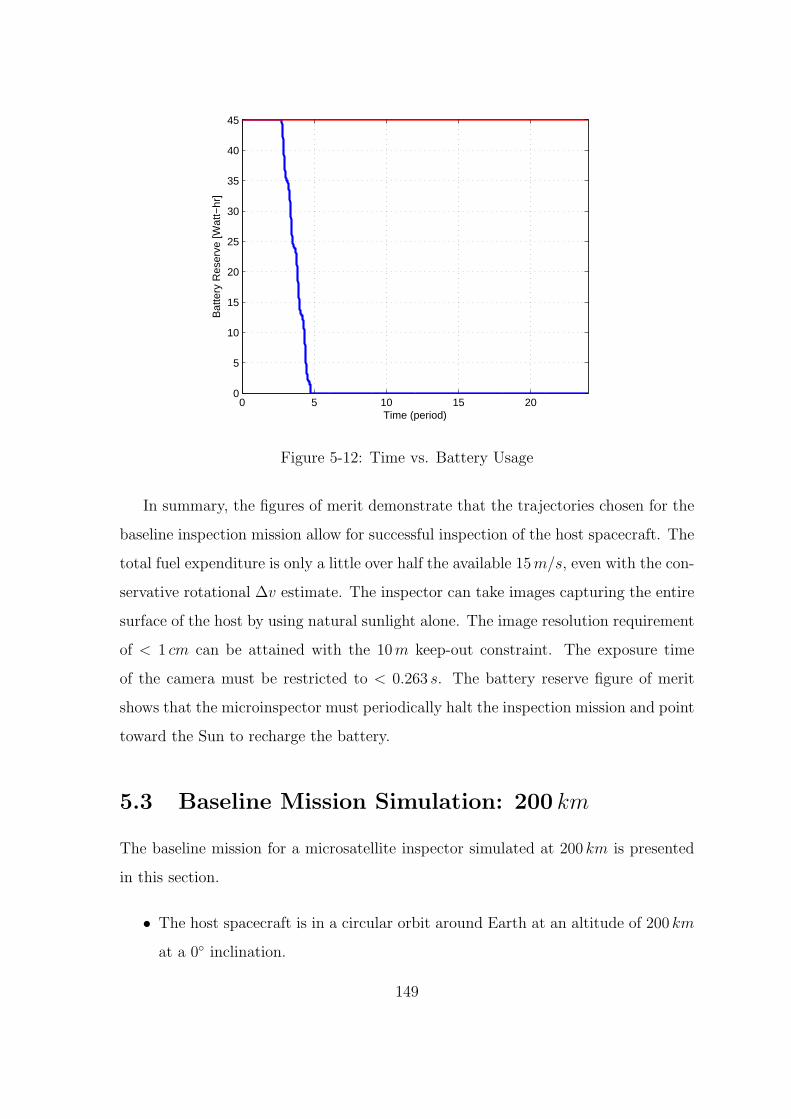
0 5 10 15 200

5

10

15

20

25

30

35

40

45

Time (period)

Bat

tery

Res

erve

[Wat

t−hr

]

Figure 5-12: Time vs. Battery Usage

In summary, the figures of merit demonstrate that the trajectories chosen for the

baseline inspection mission allow for successful inspection of the host spacecraft. The

total fuel expenditure is only a little over half the available 15m/s, even with the con-

servative rotational ∆v estimate. The inspector can take images capturing the entire

surface of the host by using natural sunlight alone. The image resolution requirement

of < 1 cm can be attained with the 10m keep-out constraint. The exposure time

of the camera must be restricted to < 0.263 s. The battery reserve figure of merit

shows that the microinspector must periodically halt the inspection mission and point

toward the Sun to recharge the battery.

5.3 Baseline Mission Simulation: 200 km

The baseline mission for a microsatellite inspector simulated at 200 km is presented

in this section.

• The host spacecraft is in a circular orbit around Earth at an altitude of 200 km

at a 0◦ inclination.

149

• The minimum distance from the surface during imaging is 10.1m, similar to

the 500 km case.

• The geocentric inertial Sun position vector is along the positive X-axis of the

geocentric inertial reference frame.

• The spirals are 4m apart, so that the images have greater than 10 pixels of

overlap, laterally.

• The total time for the inspection mission is about 35P , where 1P = 1.577hr.

The time-step for the simulation is ≈ 53 s. This does not include the disposal

mode.

The main difference between the results from this simulation at 200 km and the

previous simulation at 500 km is the fuel consumption for translational motion. All

other results are similar. The fuel expended during the entire mission for translational

motion is still less than the total available ∆v of 15m/s, as shown in Figure 5-13a.

However, the total translational ∆v is much larger when compared to Figure 5-5a.

This increase in fuel consumption is primarily due to the larger value of differential

drag at the lower altitude. The ∆v used for orbit maintenance throughout the mission

is much greater at the lower altitude. The total rotational ∆v estimate is nearly

equivalent to the 500 km case, as shown in Figure 5-13b. Figure 5-13c illustrates the

total ∆v used.

The maximum velocity magnitude during the global inspection mode at the lower

altitude is 0.0345m/s, which is slightly greater than the inspection mission at 500 km.

This translates to a camera exposure time of less than 0.246 s to attain less than one

pixel smear.

150

0 5 10 15 20 250

1

2

3

4

5

6

7

Time (period)

∆v (

m/s

)

(a) Translation ∆v

0 5 10 15 20 25 300

1

2

3

4

5

6

7

8

9

Time (period)

∆v (

m/s

)

(b) Rotational ∆v

0 5 10 15 20 25 300

5

10

15

Time (period)

∆v (

m/s

)

(c) Total ∆v

Figure 5-13: Fuel Expenditure: Time vs. ∆v

151


152

Chapter 6

Extension to Free Space

In deep space, the main source of disturbance is the gravitational or solar pressure per-

turbation from the Sun. However, because this source of perturbation is minuscule, it

is omitted in the scope of this deep space trajectory study. With this assumption, the

achievable motion about the host vehicle is contingent upon the type of trajectories

that can be designed using forced motion. Natural motion is available in the deep

space case, but highly impractical to use in designing inspection trajectories. Recall

from Section 3.1 that the time to make one revolution in a relative closed orbit about

the host vehicle is equivalent to the orbital period. In deep space, the host vehicle

is essentially orbiting the Sun. A full orbit may take years. Thus, utilizing natural

motion for designing trajectories would also take years — an infeasible option for

inspection missions. The space environment during orbital transfer trajectories (e.g.

Earth to Moon, or near Libration points) can also be considered as a deep space case.

The baseline mission for the orbiting host can be extended to this free space

representation. Much like the baseline mission simulation presented in Chapter 5 for

the orbiting host case, the camera on board the microinspector can capture a large

percentage of the host’s surface by maneuvering around the host in circular loop

motions along the length. Since the loops must be shaped by forced maneuvers, a

circular trajectory can only be achieved by continuous thrusting.

In order to conserve fuel, a polygon shaped trajectory with Np sides is considered

here. The Np-sided polygon still retains the loop-like motion about the host, which

153

proved to be advantageous for imaging. Yet, the number of ∆v burns is finite, mini-

mizing the overall fuel expenditure. Figure 6-1 displays a segment of an equal sided

polygon that could be used in shaping the inspection trajectory. rp is the radius of

the polygon, δqp is the length of one of the the polygon sides, and θp is the angle

between the radial lines.

rp

θp

ϕp

θp

rp

rp

δqp

ϕp

ϕp

ϕp

v v

δv

θp

Figure 6-1: Equal-sided Polygon

From Figure 6-1, the length of one polygon side is determined by:

δqp = 2rp sin

(

θp

2

)

(6.1)

Also from the figure, the incremental velocity magnitude to change the direction of

the velocity vector, so that it is tangential to the next leg of the polygon, is given by:

|δv| = δv = 2v sin

(

θp

2

)

(6.2)

Let T be the total time for one revolution about the polygon. Given T , Np, and rp,

the equation for θp is:

θp =2π

Np

(6.3)

Then, the total length of the polygon sides is:

qp = 2Nprp sin

(

π

Np

)

(6.4)

154

and the magnitude of the total velocity needed to make a complete revolution about

the Np-sided polygon is given by:

|∆v| = ∆v = 2Npv sin

(

π

Np

)

(6.5)

With qp and T , the magnitude of the velocity on each leg of the polygon is:

|v| = v =qpT

(6.6)

By substituting Eqn 6.6 for v into Eqn 6.5, ∆v can be rewritten as:

∆v = 2Np

2Nprp sin(

πNp

)

T

sin

(

π

Np

)

=4rp

TNp

2 sin2

(

π

Np

)

(6.7)

Eqn 6.7 is observed to have a limit, which is given by:

limNp→∞

∆v =4π2rp

T(6.8)

The size of the polygon is dictated by rp. By Eqn 6.7, it is seen that fuel use

increases linearly with respect to rp, given equivalent values for T and Np. With the

same value for T , fuel expenditure can also be expected to increase when the number

of sides is increased. However, by Eqn 6.8, a limit is reached as Np → ∞. This limit

is equal to the fuel expended traversing in a circle via continuous thrust.

155

Figure 6-2 illustrates a simulation of the trajectories generated for global inspec-

tion in deep space. Each polygon has Np = 6 sides. The trajectory around the host

vehicle has a maximum distance of rmax = 20m from the y-axis and completes one

revolution in 1hr. The total translational ∆v to conduct this part of the mission is

1.73m/s. The ∆v at each corner of the polygon to complete a revolution in 1hr has

a magnitude of 0.034m/s.

(a) 3D (b) x-z View

Figure 6-2: Deep Space Case 1: Np = 6, rmax = 20m, 1 revolution in 1hr.

156

Figure 6-3 displays the global inspection mission when the number of sides of

the polygons is increased to ten. The trajectory around the host vehicle still has a

maximum distance of rmax = 20m from the y-axis, and completes one revolution in

1hr. The total translational ∆v to complete this part of the mission is 1.88m/s.

As expected, the fuel expenditure has increased with the larger number of sides.

ChangingNp from six to ten results in a 0.15m/s increase in fuel expenditure. The ∆v

burn at each corner of the polygon to complete a revolution in 1hr takes 0.021m/s.

(a) 3D (b) x-z View

Figure 6-3: Deep Space Case 2: Np = 10, rmax = 20m, 1 revolution in 1hr.

The same figures of merit used to characterize the baseline mission in Chapter 5

may also be utilized to rate the inspection quality of the deep space microinspector

mission.

157


158

Chapter 7

Conclusions

This chapter summarizes the results of the trajectory and mission study conducted

for a microsatellite inspector.

7.1 Thesis Summary

A trajectory analysis for the mission design of a microsatellite inspector vehicle was

conducted and presented in this thesis. The study covered two mission scenarios —

Earth orbiting and deep space. For the orbiting case, a natural motion trajectory

for inspection of the host spacecraft was primarily designed utilizing the solution to

the CW equations. The key factors affecting an inspection mission were discussed

and detailed in this thesis. The relative motion space was first explored via the CW

solution. From this analysis, a toolset of trajectories that would potentially be useful

for vehicle inspection was developed. The methods, used in this thesis, for calculating

the transfer motion between these trajectories were also based on the CW solution.

A baseline mission design concept for a microinspector was presented, which con-

sisted of a deployment mode, a global inspection mode, a point inspection mode,

and a disposal mode. The 3DOF simulation of the baseline mission was based on

the trajectory toolset and transfer methods. The altitude and inclination of the host

spacecraft’s orbit about Earth had to be specified for the simulation. The attitude of

the microinspector was not simulated; however, the fuel usage by the attitude control

159

system was estimated by assuming an angular position bang-bang controller. Fac-

tors that could be used to score the successfulness of an inspection mission were also

outlined. These figures of merit were used to show the effectiveness of the chosen

baseline inspection mission. The hardware requirements and constraints employed in

the simulation were based on JPL’s microinspector design.

Simulations of the baseline inspection mission were conducted for LEO at altitudes

of 500 km and 200 km. The main conclusion for these scenarios was that the attitude

motion consumed considerably more fuel than the translational motion at altitudes

higher than 200 km. The total available ∆v of 15m/s was found to be more than

adequate for the entire mission at both altitudes. In order to accurately estimate the

fuel expenditure for attitude control, it is recommended that a six-degree-of-freedom

simulation of the microinspector’s orbital motion and attitude be developed, with

fuel optimizing attitude control techniques. It was determined that to complete the

inspection mission, the microinspector needs to periodically take time out of its in-

spection tasks and recharge the batteries by pointing at the Sun. The simulated

baseline mission was able to attain image resolutions that were less than or equal

to the desired maximum resolution of 1 cm, during the global inspection and point

inspection mode. The minimum distance avoidance constraint of 10m was not vio-

lated in achieving this imaging goal. The maximum relative velocity magnitude for

both the 500 km and 200 km altitude cases in the baseline mission simulation showed

that the camera exposure time should be less than 0.5 s to achieve less than one pixel

smear.

In the deep space scenario, the natural motion dynamics were found to be too

slow to be useful. Forced motion was employed to design the trajectories for this

case. Because the spiraling motion – which was employed in the Earth orbiting

scenario – proved to be advantageous for capturing images of the complete surface of

the host, a similar concept was used in the deep space scenario. An Np-sided polygon

was utilized to mimic the looping motion about the host vehicle. Given a constant

revolution time, it was shown that an increase in the number of sides correlated

directly with an increase in fuel expenditure. As N approaches infinity, the shape of

160

the polygon approaches a circle. The ∆v amount also approaches the total ∆v for

continuous thrusting in a circle about the host vehicle. The global inspection concept

utilizing the polygon method of trajectory design was shown in this thesis.

7.2 Future Work

In this thesis, the attitude of the microinspector was not explicitly simulated. In order

to better understand the coupling effects between the orbital and attitude dynamics,

the author recommends a full six-degree-of-freedom simulation be developed and an-

alyzed, using the baseline inspection mission presented in this thesis. A Sun-nadir

angular position controller can be specifically implemented to accurately estimate the

fuel costs and battery usage.

Additionally, a trades-analysis on the different microinspector hardware specifica-

tions for the baseline mission is needed. Depending on the microinspector’s design,

the trajectories for an inspection mission may vary drastically from the baseline mis-

sion discussed in this thesis. The baseline mission simulation must also be conducted

for host vehicles at higher altitudes, to test the effectiveness of the inspection trajec-

tories.

From the results of the baseline mission simulation, it was concluded that the

rotational ∆v for attitude control was the main source of fuel consumption in Earth

orbiting scenarios at altitudes > 200 km. Since a continuous Sun-nadir pointing

scheme requires complicated attitude maneuvers, this translates directly to high fuel

consumption. This continuous charging method may not even be necessary depending

on the capacity of the battery. Thus, there is an obvious need for a trade study

between continuous charging via the Sun-nadir pointing algorithm and periodically

taking time out from the inspection mission to point the solar cells at the Sun.

Only a cylindrical-shaped model of a host spacecraft was used in the baseline

mission simulation. Further studies need to be conducted utilizing a range of differ-

ent host spacecraft models. Another important case to be examined is if the host

spacecraft is rotating or tumbling in the LVRCS.

161

The different spacecraft models and hardware specifications will affect the value

for differential drag. The constant differential drag assumption is no longer valid when

the attitude of the host spacecraft and microinspector are continuously changing in

the LVRCS. Thus, a model of the differential drag that accounts for these changing

values is needed.

The simulations in this thesis only used the box keep-out zone in developing the

trajectories. There are many other keep-out zone models that can be implemented

with the simulations, such as a spherical or cylindrical model keep-out zone. These

avoidance constraints can be integrated with the trajectory designs from this thesis.

For irregularly shaped host vehicles, more attention needs to be given to avoiding the

keep-out zone during transfer planning.

The baseline mission simulation presented here can be extended to other planet

orbiting scenarios. The gravitational, solar, and atmospheric disturbances may differ

significantly from the Earth orbiting case, which directly affects fuel expenditure,

battery usage, and imaging. Furthermore, the deep space mission concept presented

in this thesis needs to be simulated, as in the Earth orbiting case. The same figures

of merit can be applied to describe the quality of the inspection mission designed for

the host in consideration.

Each figure of merit needs to be assigned a weighting factor, when rating the

inspection mission. The weighting factor depends on the type of host vehicle, as well

as the goals of the mission. A study on how to develop the weighting factors must

be carried out in order to determine the best inspection mission for a particular host

vehicle.

162

Appendix A

Characterization of all Closed

Relative Orbits

If X0 is zero, then the relative motion appears to stay stationary in the LVRCS. This

stationary relative motion will be referred to as a closed relative orbit throughout

this thesis. All closed relative orbits have a period equal to the orbital period of

the host vehicle. This fact is readily supported by the CW solution. Given the

value of the semiminor axis, b, a 2×1 elliptical cylinder, whose length is in the z-axis,

can be defined. The closed relative orbits that can be achieved may be described

by plane slices through this 2×1 elliptical cylinder and the desired Y0, as illustrated

conceptually in Figure A-1. Consequently, the closed relative orbit cannot expressly

be in the x-z or y-z plane in the LVRCF.

163

x

y

z

Figure A-1: Plane Slice through 2×1 Elliptical Cylinder

Each closed relative orbit can be characterized by its normal vector, which is

parallel to the “angular momentum” direction of the relative motion. Two angles, α

and β, can be used to define this unit normal vector. Thus, all closed relative orbits

can also be characterized by these two angles alone. The normal vector and the two

angles are measured from the center of the closed relative orbits. Figure A-2 shows a

diagram of a 2×1 elliptical cylinder, a unit normal vector, and a graphical depiction

of the α and β angles.

x

y

z

α

β

û

Figure A-2: Characterization of Closed Relative Orbits

164

To correlate the α and β angles with the parameters of the traveling ellipse for-

mulation of the CW solution, notice that the equation for the relative orbit’s angular

momentum vector may be employed in place of the unit normal vector. Recalling the

equations for r and v from Eqn 3.8 and Eqn 3.9, the traveling ellipse formula for the

initial position, r0, and velocity, v0, for a closed relative orbit may be obtained by

setting t = 0 and X0 = 0. Simplifying further, Y0 is set to zero, since the two angles

are measured from the center of the closed orbit, and the differential accelerations

are set to zero. Applying this set of values gives the following formula for r0 and v0:

r0 =

x0

y0

z0

=

b sin(φ)

2b cos(φ)

c sin(ψ)

(A.1)

v0 =

x0

y0

z0

=

bω cos(φ)

−2bω sin(φ)

cω cos(ψ)

(A.2)

The angular momentum vector, h, at t = 0 is given by:

h = r0 × v0 =

∣

∣

∣

∣

∣

∣

∣

∣

∣

i j k

b sin(φ) 2b cos(φ) c sin(ψ)

bω cos(φ) 2bω sin(φ) cω cos(ψ)

∣

∣

∣

∣

∣

∣

∣

∣

∣

=

2bcω cos(φ− ψ)

−bcω sin(φ− ψ)

−2b2ω

=

hx

hy

hz

(A.3)

The α and β angles characterizing this closed relative orbit can be determined geo-

metrically from the angular momentum terms in Eqn A.3.

165

tan(α) = −hz

hy

=−2b2ω

−bcω sin(φ− ψ)=

2b

c sin(φ− ψ)(A.4)

tan(β) =hx

√

h2y + h2

z

=2bcω cos(φ− ψ)

√

(−bcω sin(φ− ψ))2 + (−2b2ω)2

=2c cos(φ− ψ)

√

c2 sin2(φ− ψ) + 4b2(A.5)

From Eqn A.4 and Eqn A.5, equations that correlate the α and β angles with (φ−ψ)

and c can be found:

tan(φ− ψ) = 2cos(α)

tan(β)(A.6)

c =b

sin(α)

√

tan2(β) + 4 cos2(α) (A.7)

Therefore, if the unit normal of the desired closed loop, or the desired α and β angles

are known, the constraint for φ and ψ, and the out-of-plane amplitude c can be

calculated for a chosen b and vice versa.

By inspection and also as an outcome of Eqn A.6–A.7, there exists some con-

straints on the α and β angles, shown in Eqn A.8–A.9.

α 6= 0, π (A.8)

β 6= 0,±π2

(A.9)

166

Appendix B

Relationship Between CW

Solution Parameters and Orbital

Elements

The CW solution is based on a host vehicle that is in a circular orbit about the

planet. If the secondary vehicle’s orbit is in the same orbital plane as the host, then

the orbital elements describing this orbit can easily be related to the CW solution

parameters. A full description of the orbital elements can be found in Chapter 3

of Battin’s An Introduction to the Mathematics and Methods of Astrodynamics [19].

Given the semiminor axis of a 2×1 elliptical relative orbit, b′, and the radius of

the host’s circular orbit, rh, the orbital elements of the microinspector’s orbit about

the planet can be determined. The computation of a few of these orbital elements

relating to the traveling ellipse parameters is discussed in this section. Table B.1 gives

a description of these orbital elements.

167

Table B.1: Description of Orbital Elements

Parameter Description

a Semimajor axis of microinspector’s orbitb Semiminor axis of microinspector’s orbite Eccentricity of microinspector’s orbitrp Pericenter radiusra Apocenter radiusrh Radius of host’s circular orbit

Figure B-1 shows the orbits of the host and microinspector about the Earth. The

microinspector’s orbit correlates to a 2×1 ellipse in the LVRCS. The size of the orbits

is exaggerated in the figure to elucidate the parameter descriptions.

Microinspector’s

OrbitHost Vehicle’s

Orbit

b‘ b‘

b

rh

a

ra

rp

Figure B-1: Secondary Vehicle’s Orbital Elements

As shown in Figure B-1, the relationship between the 2×1 ellipse’s semiminor axis,

b′, and the radius of the the host orbit’s circular orbit, rh, to the pericenter radius,

rp, and apocenter radius, ra, is given by:

rp = rh − b′ (B.1)

ra = rh + b′ (B.2)

168

The formulas relating rp and ra to the orbit’s semimajor axis, a, and semiminor axis,

b are given by:

a =1

2(rp + ra) (B.3)

b =√rpra (B.4)

Substituting Eqn B.1–B.2 into Eqn B.3 and Eqn B.4,

a =1

2(rp + ra)

=1

2(rh − b′ + rh + b′)

= rh (B.5)

and

b =√rpra

=√

(rh − b′) (rh + b′)

=√

r2h − b′2 (B.6)

Also, from the formula relating b, a, and the eccentricity, e, shown by Eqn B.7, a

relationship between b, b′, and rh can be found.

b2 =∣

∣a2(

1 − e2)∣

∣ (B.7)

Substituting the results of Eqn B.5–B.6 into Eqn B.7, the following relation is found:

e2 = 1 − b2

a2=b′2

r2h

(B.8)

The period of an elliptical orbit about a planet may be obtained by applying

169

Kepler’s second law, which gives the time required for the radius vector to sweep over

the entire enclosed area. The equation for the period is given by:

P = 2π

√

a3

µ(B.9)

where µ is the gravitational parameter of the planet.

Since the semimajor axis of the microinspector’s orbit is equal to the radius length

of the host’s circular orbit, by Eqn B.5, the orbital period is the same for the host

and the microinspector. Thus, all closed relative orbits of the microinspector about

the host has the same period as the orbital period of the host and microinspector.

The magnitude of the velocity at any given point on the orbit can be determined

from the energy integral, sometimes called the vis-viva integral, which is given by

Eqn B.10.

v2 = µ

(

2

r− 1

a

)

(B.10)

The vis-viva integral reveals the relationship between the velocity magnitude and

the semimajor axis, a. In Section 3.1.2, it was stated that for a traveling ellipse, the

secondary vehicle appears to move forward or backward in relation to the host vehicle

because its velocity is greater than or less than that of the host, respectively. This

statement is validated by Eqn B.10. a is the same for both orbits by Eqn B.5. If r for

the microinspector’s orbit is greater than rh, then the magnitude of the velocity will

be less. Thus, the microinspector will move backward relative to the host vehicle due

to the lesser velocity. Conversely, if r is less than rh, then the velocity magnitude will

be greater. Hence, the microinspector moves faster than the host vehicle, appearing

to move forward.

In Figure B-2, the velocity vectors of the host and microinspector are illustrated

in the LVRCS, where the host is centered at the origin. rh is the position vector

from the Earth to the host vehicle in the geocentric reference frame. ω is the orbital

velocity of the host. vh is the velocity vector of the host and vi is the velocity vector

of the microinspector, both in the geocentric reference frame. ∆vi is the velocity

170

vector of the microinspector in the LVRCS.

x

yHost

rh

ω

vh

vh

vi

∆vi

Microinspector

Figure B-2: Velocity of Host and Inspector in LVRCS

The host vehicle’s velocity vector is given by:

vh = ω × rh (B.11)

One can also interpret the host’s velocity as the velocity of the origin of the

LVRCS. Therefore, the microinspector’s total velocity, vi, is just the sum of the host’s

velocity (velocity of the origin of the LVRCS) and the velocity of the microinspector

relative to the host vehicle.

Let vi = [vx, vy, vz]. Then, from Figure B-2, we see that vy will primarily be

composed of vh. In the 2×1 ellipse, this is the largest factor in the microinspector’s

total velocity, which implies that vy >> vx, vz,∆v. The calculations below show the

magnitude of the microinspector’s total velocity after ∆v is applied separately along

the x-axis and y-axis in the LVRCS. For ∆v applied along the x-axis,

171

v =

√

(vx + ∆v)2 + vy2 + vz

2 =√

vx2 + 2vx∆v + ∆v2 + vy

2 + vz2 (B.12)

For ∆v applied along the y-axis,

v =

√

vx2 + (vy + ∆v)2 + vz

2 =√

vx2 + vy

2 + 2vy∆v + ∆v2 + vz2 (B.13)

Comparing the two results, it is apparent that the magnitude of the total velocity is

optimally changed when ∆v is applied parallel to the V-bar, since 2vy∆v >> 2vx∆v.

Directing ∆v in any other direction decreases the variation in magnitude. Thus, to

conserve fuel when changing the forwards or backwards motion of the microinspec-

tor in relation to the host, the impulse velocity, ∆v, must be applied parallel to the

V-bar (y-axis) in the LVRCS. Applying ∆v in this manner will effectively change the

semimajor axis, a, and consequently the period, determined from Eqn B.9. More

specifically, applying ∆v in the positive y-direction increases a, and the 2×1 ellipse

travels in the negative y-direction. Applying ∆v in the negative y-direction decreases

a, and the 2×1 ellipse travels in the positive y direction. Figure B-3–B-4 illustrate

these findings. Figure B-3 shows the resulting motion when ∆v =0.01m/s is ap-

plied when φ = 0◦ on the 2×1 ellipse. Figure B-4 shows the resulting motion when

∆v =0.01m/s is applied when φ = 90◦ on the 2×1 ellipse. The 2×1 ellipse about the

host vehicle has a semiminor axis of 20m.

172

−500−400−300−200−1000−200

−150

−100

−50

0

50

100

150

200

y [m]

x [m

]

2x1 ellipse∆v applied parallel to V−bar∆v applied perpendicular to V−bar

Figure B-3: ∆v applied when φ = 0◦

−500−400−300−200−1000

−200

−150

−100

−50

0

50

100

150

200

y [m]

x [m

]

2x1 ellipse∆v applied parallel to V−bar∆v applied perpendicular to V−bar

Figure B-4: ∆v applied when φ = 90◦

173

For both figures, when ∆v is applied in the positive y-direction, the semimajor

axis, a, and the period of the microinspector’s orbit about Earth are increased, causing

the microinspector to appear as if it is moving behind the host in the LVRCS. When

∆v is applied in the positive x-direction, a and the period are also increased in this

case, but by a significantly smaller amount. X0 is not changed for this particular

orbit because the relative initial velocity on the y-axis (y0) is unchanged. However,

Y0 and b′ are changed due to the difference in initial velocity along the x-axis (x0).

Refer to Eqn 3.11 for descriptions of the traveling ellipse parameters‡.

‡Note that b in Eqn 3.11 is the same as b′ used here. b is used for the semiminor axis of the

microinspector’s orbit about the Earth in this section.

174

Appendix C

Acronyms

ISS – International Space Station

CEV – Crew Exploration Vehicle

GN&C – Guidance, Navigation, and Control

SSC – Surrey Space Centre

SSTL – Surrey Satellite Technology Limited

SNAP-1 – Surrey Nanosatellite Applications Platform

AFRL – Air Force Research Laboratory

JPL – Jet Propulsion Laboratory

Mini-AERcam – Miniature Autonomous Extravehicular Robotic Camera

JSC – NASA Johnson Space Center

LEO – Low Earth Orbit

CW – Clohessy-Wiltshire

IMU – Inertial Measurement Unit

ACS – Attitude Control System

LVLH – Local-vertical Local-horizontal

LVRCS – Local-vertical Rotating Coordinate System

SOC – State of Charge

FOV – Field of View

175


176

Bibliography

[1] S. E. Fredrickson, L. W. Abbott, S. Duran, J. D. Jochim, J. W. Studak, J. D. Wa-

genknecht, and N. M. Williams, “Mini AERCam: Development of a Free Flying

Nanosatellite Inspection Robot,” in Space Systems Technology and Operations,

ser. SPIE, vol. 5088, Orlando, FL, Apr. 24, 2003, pp. 97–111.

[2] J. G. Macke, D. P. Miller, M. A. Swartwout, K. J. Bennett, and W. D. Smart,

“Deployable Inspector Spacecraft for Distributed Field Measurements,” in 22nd

AIAA International Communications Satellite Systems Conference and Exhibit

2004, Monterey, CA, May 9-12, 2004, paper AIAA 2004-3152.

[3] A. Jacobovits and T. W. Vaneck, “AeroAstro’s Escort - A Microsatellite for On-

Orbit Inspection of Space Assets,” in 17th Annual AIAA/USU Conference on

Small Satellites, Logan, UT, 2003.

[4] C. Underwood, G. Richardson, and J. Savignol, “SNAP-1: A Low Cost Modular

COTS-based Nano-satellite – Design, Construction, Launch and Eearly Opera-

tions Phase,” in 15th AIAA/USU Conference on Small Satellites, Logan, UT,

Aug.13-16, 2001.

[5] W. H. Steyn and Y. Hashida, “In-orbit Attitude Performance of the 3-axis Sta-

bilised SNAP-1 Nanosatellite,” in 15th AIAA/USU Conference on Small Satel-

lites, Logan, UT, Aug.13-16, 2001.

[6] D. Gibbon and C. Underwood, “Low Cost Butane Propulsion Systems for Small

Spacecraft,” in 15th AIAA/USU Conference on Small Satellites, Logan, UT,

Aug.13-16, 2001.

177

[7] R. Lancaster and C. Underwood, “SNAP-1 Machine Vision System,” in

AIAA/USU Annual Conference on Small Satellites, 12th, Logan, UT, Aug.21-24,

2000.

[8] “XSS-10 Microsatellite Flight Demonstration Program,” AFRL Technology Hori-

zons, vol. 5, pp. 10–12, Dec. 2004.

[9] “XSS-10 Micro Satellite,” http://www.vs.afrl.af.mil/, Feb. 2005, date of Access:

Mar 16, 2006.

[10] “XSS-11 Micro Satellite,” http://www.vs.afrl.af.mil/, Dec. 2005, date of Access:

Mar 16, 2006.

[11] J. Mueller, H. Goldberg, and L. Alkalai, “Micro-Inspector Spacecraft for Space

Exploration Missions and Beyond,” in Space Technology & Applications Inter-

national Forum, Albequerque, NM, Feb.14, 2006.

[12] S. E. Fredrickson, S. Duran, and J. D. Mitchell, “Mini AERCam Inspection

Robot for Human Space Missions,” in Space 2004 Conference and Exhibit, San

Diego, CA, Sept.28-30, 2004, paper AIAA Paper 2004-5843, pp. 1–9.

[13] “Space Systems Labs: CUSat Satellite Project,” http://cusat.cornell.edu/, date

of Access: Mar 17, 2006.

[14] M. Swartwout, J. Macke, K. Bennett, and W. Smart, “The Bandit: An Au-

tomated Vision-Navigated Inspector Spacecraft,” in 17th Annual AIAA/USU

Conference on Small Satellites, Logan, UT, 2003.

[15] A. Richards, T. Schouwenaars, J. P. How, and E. Feron, “Spacecraft Trajec-

tory Planning with Avoidance Constraints Using Mixed-Integer Linear Program-

ming,” Journal of Guidance, Control, and Dynamics, vol. 25, no. 4, pp. 755–764,

July 2002.

[16] W. H. Clohessy and R. S. Wiltshire, “Terminal Guidance System for Satellite

Rendezvous,” Journal of the Aerospace Sciences, vol. 27, no. 9, pp. 653–658,

1960.

178

[17] D. A. Vallado, Fundamentals of Astrodynamics and Applications, 2nd ed. El

Segundo, CA: Microcosm Press, 2001.

[18] S. W. Shepperd, “Constant Covariance in Local Vertical Coordinates for Near-

Circular Orbits,” Journal of Guidance, Control, and Dynamics, vol. 14, no. 6,

pp. 1318–1322, Nov.–Dec. 1991.

[19] R. H. Battin, An Introduction to the Mathematics and Methods of Astrodynamics,

revised ed. Reston, VA: AIAA, 1999.

179

Mission Design and Trajectory Analysis for Inspection of...

Documents

Transcript of Mission Design and Trajectory Analysis for Inspection of...