Missing Data & How to Deal: An overview of missing...
45
Missing Data & How to Deal: An overview of missing data Melissa Humphries Population Research Center
Transcript of Missing Data & How to Deal: An overview of missing...

Missing Data & How to Deal: An
overview of missing data
Melissa Humphries
Population Research Center
Goals
Discuss ways to evaluate and understand missing data
Discuss common missing data methods
Know the advantages and disadvantages of common
methods
Review useful commands in Stata for missing data
General Steps for Analysis with Missing
Data
1. Identify patterns/reasons for missing and recode
correctly
2. Understand distribution of missing data
3. Decide on best method of analysis
Step One: Understand your data
Attrition due to social/natural processes
Example: School graduation, dropout, death
Skip pattern in survey
Example: Certain questions only asked to respondents who
indicate they are married
Intentional missing as part of data collection process
Random data collection issues
Respondent refusal/Non-response

Find information from survey
(codebook, questionnaire)
Identify skip patterns and/or sampling strategy from documentation
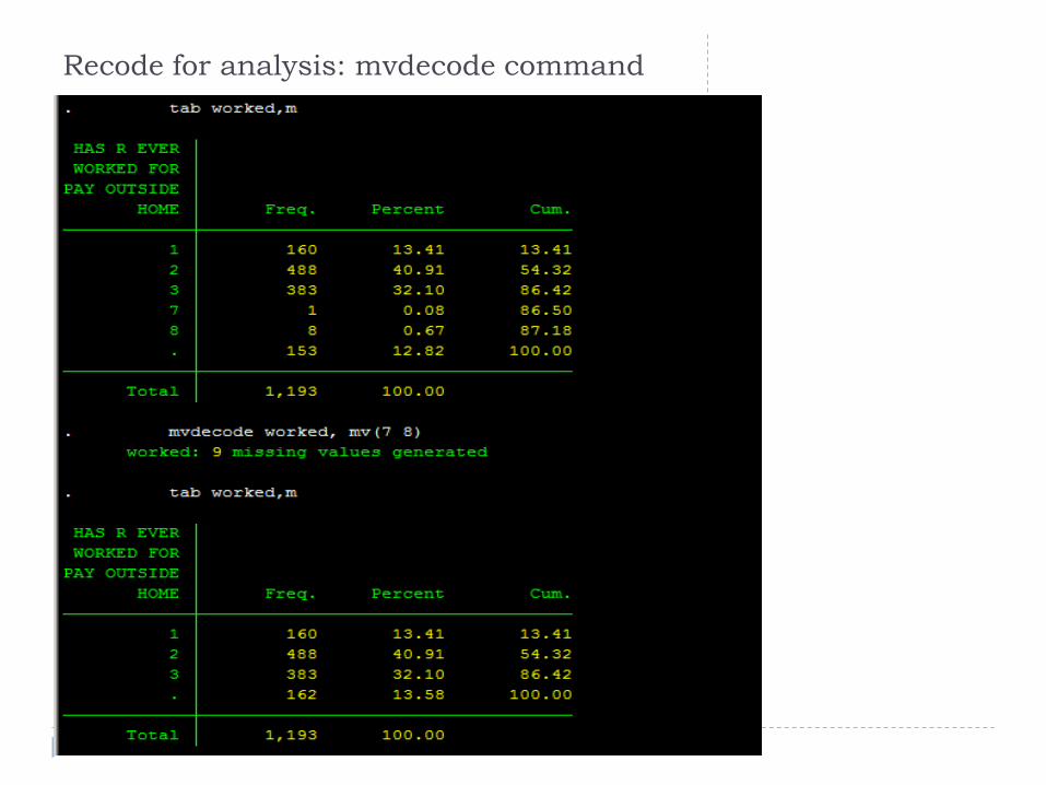
Recode for analysis: mvdecode command
Mvdecode
How stata reads missing
Tip .>#‟s
Nmissing npresent
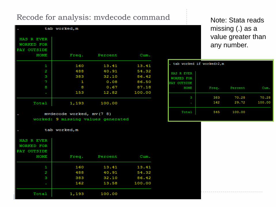
Recode for analysis: mvdecode command
Mvdecode
How stata reads missing
Tip .>#‟s
Nmissing npresent
Note: Stata reads
missing (.) as a
value greater than
any number.
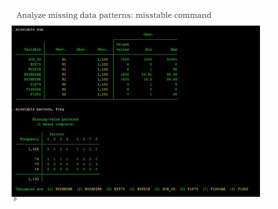
Analyze missing data patterns: misstable command
Step Two: Missing data Mechanism (or
probability distribution of missingness)
Consider the probability of missingness
Are certain groups more likely to have missing values?
Example: Respondents in service occupations less likely to report
income
Are certain responses more likely to be missing?
Example: Respondents with high income less likely to report income
Certain analysis methods assume a certain probability
distribution

Missing Data Mechanisms
Missing Completely at Random (MCAR)
Missing value (y) neither depends on x nor y
Example: some survey questions asked of a simple random
sample of original sample
Missing at Random (MAR)
Missing value (y) depends on x, but not y
Example: Respondents in service occupations less likely to report
income
Missing not at Random (NMAR)
The probability of a missing value depends on the variable that
is missing
Example: Respondents with high income less likely to report income

Exploring missing data mechanisms
Can‟t be 100% sure about probability of missing (since we
don‟t actually know the missing values)
Could test for MCAR (t-tests)—but not totally accurate
Many missing data methods assume MCAR or MAR but
our data often are MNAR
Some methods specifically for MNAR
Selection model (Heckman)
Pattern mixture models

Good News!!
Some MAR analysis methods using MNAR data are still
pretty good.
May be another measured variable that indirectly can predict
the probability of missingness
Example: those with higher incomes are less likely to report income
BUT we have a variable for years of education and/or number of
investments
ML and MI are often unbiased with NMAR data even though
assume data is MAR
See Schafer & Graham 2002

Step 3: Deal with missing data
Use what you know about
Why data is missing
Distribution of missing data
Decide on the best analysis strategy to yield the least
biased estimates
Deletion Methods
Listwise deletion, pairwise deletion
Single Imputation Methods
Mean/mode substitution, dummy variable method, single regression
Model-Based Methods
Maximum Likelihood, Multiple imputation
Deletion Methods
Listwise deletion
AKA complete case analysis
Pairwise deletion

Listwise Deletion (Complete Case Analysis)
Only analyze cases with
available data on each
variable
Advantages:
Simplicity
Comparability across
analyses
Disadvantages:
Reduces statistical power
(because lowers n)
Doesn‟t use all information
Estimates may be biased if
data not MCAR*
Gender 8th grade math
test score
12th grade
math score
F 45 .
M . 99
F 55 86
F 85 88
F 80 75
. 81 82
F 75 80
M 95 .
M 86 90
F 70 75
F 85 .
*NOTE: List-wise deletion often produces unbiased regression slope estimates as long as
missingness is not a function of outcome variable.

Application in Stata
Any analysis including multiple variables automatically
applies listwise deletion.
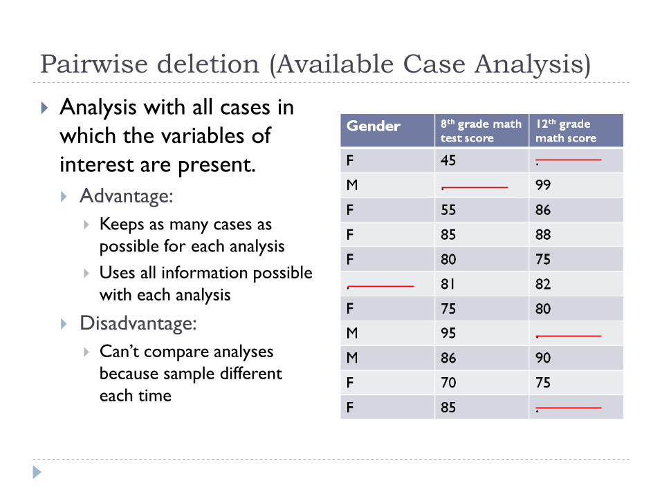
Pairwise deletion (Available Case Analysis)
Analysis with all cases in
which the variables of
interest are present.
Advantage:
Keeps as many cases as
possible for each analysis
Uses all information possible
with each analysis
Disadvantage:
Can‟t compare analyses
because sample different
each time

Single imputation methods
Mean/Mode substitution
Dummy variable control
Conditional mean substitution

Mean/Mode Substitution
Replace missing value with sample mean or mode
Run analyses as if all complete cases
Advantages:
Can use complete case analysis methods
Disadvantages:
Reduces variability
Weakens covariance and correlation estimates in the data (because
ignores relationship between variables)

20
40
60
80
12
th g
rade m
ath
test
sco
re
20 30 40 50 60 708th grade math test score
imputed 12th grade math test score (mean sub)

Dummy variable adjustment
Create an indicator for missing value (1=value is missing
for observation; 0=value is observed for observation)
Impute missing values to a constant (such as the mean)
Include missing indicator in regression
Advantage:
Uses all available information about missing observation
Disadvantage:
Results in biased estimates
Not theoretically driven
NOTE: Results not biased if value is missing because of a
legitimate skip

Regression Imputation
Replaces missing values with predicted score from a
regression equation.
Advantage:
Uses information from observed data
Disadvantages:
Overestimates model fit and correlation estimates
Weakens variance

20
40
60
80
12
th g
rade m
ath
test
sco
re
20 30 40 50 60 708th grade math test score
imputed 12th grade math test score (single regression)
Model-based methods
Maximum Likelihood
Multiple imputation

Model-based Methods: Maximum Likelihood
Estimation
Identifies the set of parameter values that produces the highest log-likelihood.
ML estimate: value that is most likely to have resulted in the observed data
Conceptually, process the same with or without missing data
Advantages:
Uses full information (both complete cases and incomplete cases) to calculate log likelihood
Unbiased parameter estimates with MCAR/MAR data
Disadvantages
SEs biased downward—can be adjusted by using observed information matrix

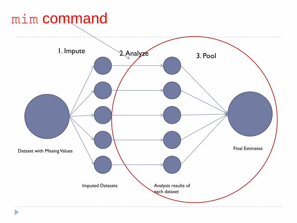
Multiple Imputation
1. Impute: Data is „filled in‟ with imputed values using
specified regression model
This step is repeated m times, resulting in a separate dataset
each time.
2. Analyze: Analyses performed within each dataset
3. Pool: Results pooled into one estimate
Advantages:
Variability more accurate with multiple imputations for each missing
value
Considers variability due to sampling AND variability due to imputation
Disadvantages:
Cumbersome coding
Room for error when specifying models

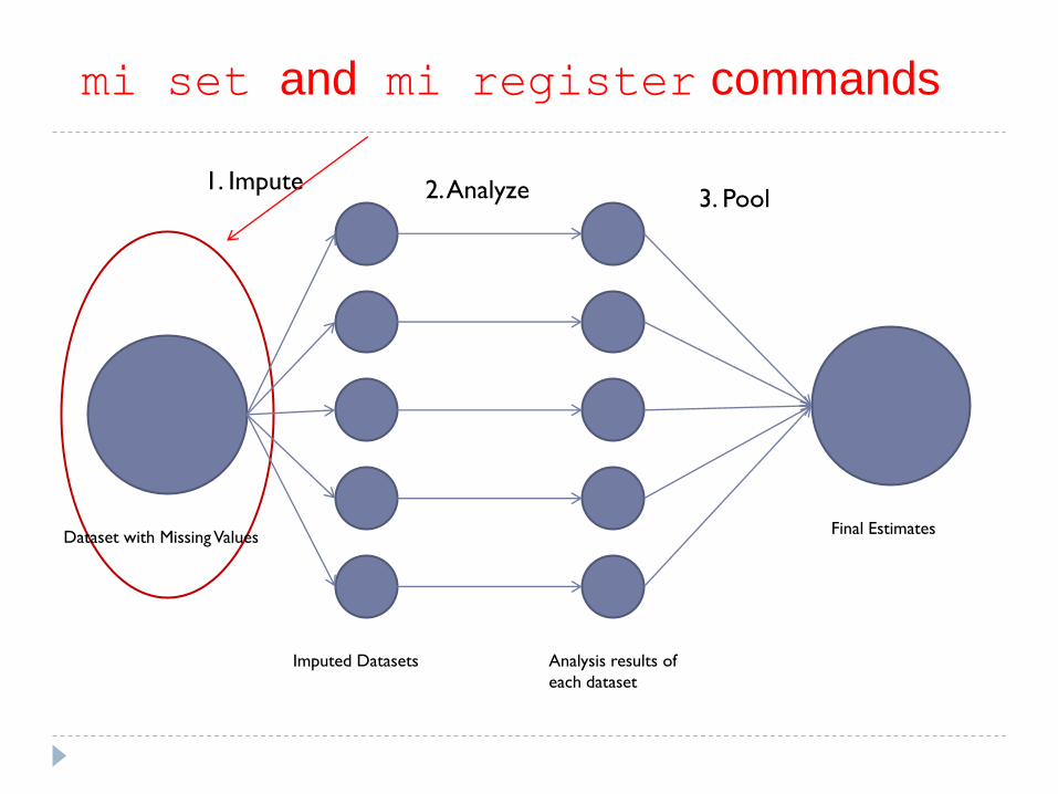
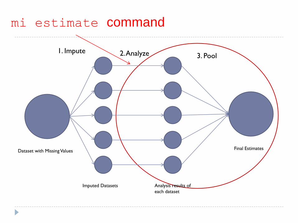
Multiple Imputation Process
Dataset with Missing Values
Imputed Datasets Analysis results of
each dataset
Final Estimates
1. Impute 2. Analyze 3. Pool

Multiple Imputation: Stata & SAS
SAS:
Proc mi
Stata:
ice (imputation using chained equations) & mim (analysis with
multiply imputed dataset)
mi commands
mi set
mi register
mi impute
mi estimate
NOTE: the ice command is the only chained equation method
until Stata12. Chained equations can be used as an option of
mi impute since Stata12.

ice & mim
ice: Imputation using chained equations
Series of equations predicting one variable at a time
Creates as many datasets as desired
mim: prefix used before analysis that performs analyses
across datasets and pools estimates

Dataset with Missing Values
Imputed Datasets Analysis results of
each dataset
Final Estimates
1. Impute 2. Analyze 3. Pool
ice command
Dataset with Missing Values
Imputed Datasets Analysis results of
each dataset
Final Estimates
1. Impute 2. Analyze 3. Pool
mim command
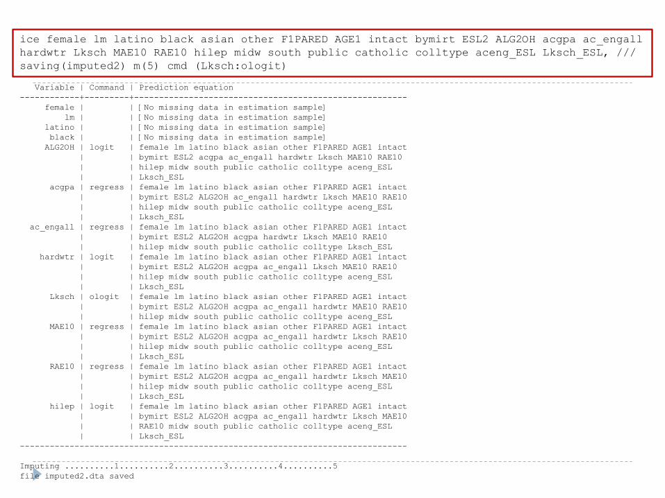
ice female lm latino black asian other F1PARED AGE1 intact bymirt ESL2 ALG2OH acgpa ac_engall
hardwtr Lksch MAE10 RAE10 hilep midw south public catholic colltype aceng_ESL Lksch_ESL, ///
saving(imputed2) m(5) cmd (Lksch:ologit)
Variable | Command | Prediction equation
------------+---------+-------------------------------------------------------
female | | [No missing data in estimation sample]
lm | | [No missing data in estimation sample]
latino | | [No missing data in estimation sample]
black | | [No missing data in estimation sample]
ALG2OH | logit | female lm latino black asian other F1PARED AGE1 intact
| | bymirt ESL2 acgpa ac_engall hardwtr Lksch MAE10 RAE10
| | hilep midw south public catholic colltype aceng_ESL
| | Lksch_ESL
acgpa | regress | female lm latino black asian other F1PARED AGE1 intact
| | bymirt ESL2 ALG2OH ac_engall hardwtr Lksch MAE10 RAE10
| | hilep midw south public catholic colltype aceng_ESL
| | Lksch_ESL
ac_engall | regress | female lm latino black asian other F1PARED AGE1 intact
| | bymirt ESL2 ALG2OH acgpa hardwtr Lksch MAE10 RAE10
| | hilep midw south public catholic colltype Lksch_ESL
hardwtr | logit | female lm latino black asian other F1PARED AGE1 intact
| | bymirt ESL2 ALG2OH acgpa ac_engall Lksch MAE10 RAE10
| | hilep midw south public catholic colltype aceng_ESL
| | Lksch_ESL
Lksch | ologit | female lm latino black asian other F1PARED AGE1 intact
| | bymirt ESL2 ALG2OH acgpa ac_engall hardwtr MAE10 RAE10
| | hilep midw south public catholic colltype aceng_ESL
MAE10 | regress | female lm latino black asian other F1PARED AGE1 intact
| | bymirt ESL2 ALG2OH acgpa ac_engall hardwtr Lksch RAE10
| | hilep midw south public catholic colltype aceng_ESL
| | Lksch_ESL
RAE10 | regress | female lm latino black asian other F1PARED AGE1 intact
| | bymirt ESL2 ALG2OH acgpa ac_engall hardwtr Lksch MAE10
| | hilep midw south public catholic colltype aceng_ESL
| | Lksch_ESL
hilep | logit | female lm latino black asian other F1PARED AGE1 intact
| | bymirt ESL2 ALG2OH acgpa ac_engall hardwtr Lksch MAE10
| | RAE10 midw south public catholic colltype aceng_ESL
| | Lksch_ESL
------------------------------------------------------------------------------
Imputing ..........1..........2..........3..........4..........5
file imputed2.dta saved
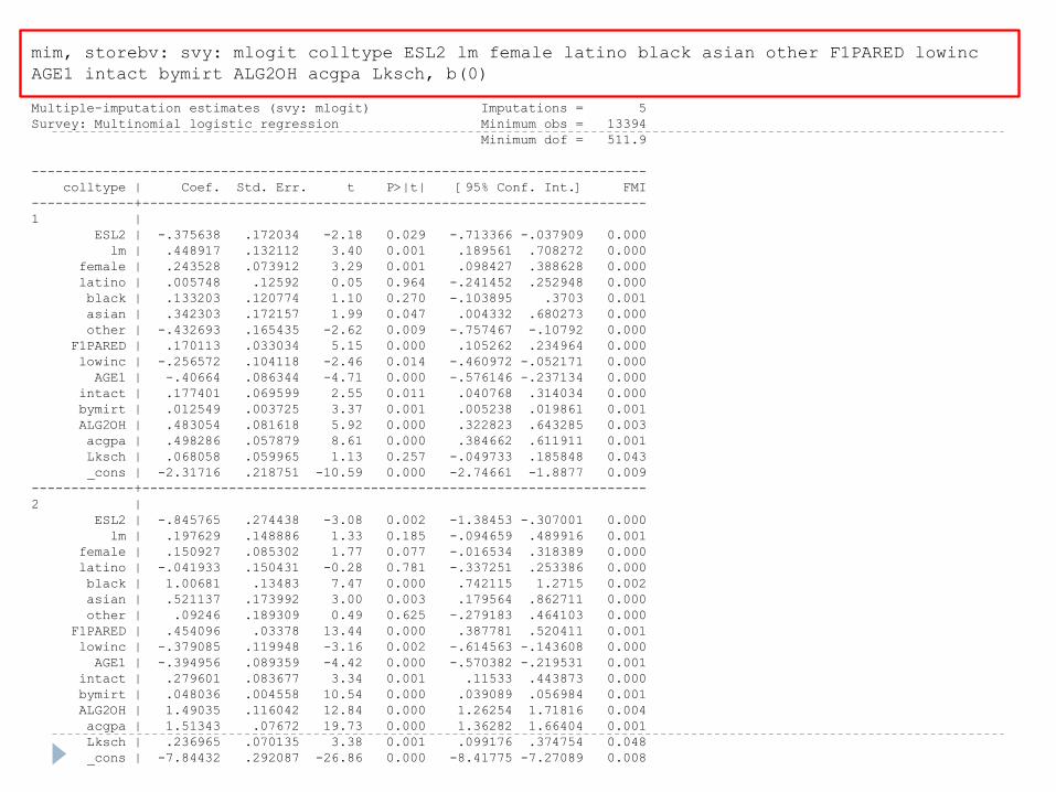
mim, storebv: svy: mlogit colltype ESL2 lm female latino black asian other F1PARED lowinc
AGE1 intact bymirt ALG2OH acgpa Lksch, b(0)
Multiple-imputation estimates (svy: mlogit) Imputations = 5
Survey: Multinomial logistic regression Minimum obs = 13394
Minimum dof = 511.9
------------------------------------------------------------------------------
colltype | Coef. Std. Err. t P>|t| [95% Conf. Int.] FMI
-------------+----------------------------------------------------------------
1 |
ESL2 | -.375638 .172034 -2.18 0.029 -.713366 -.037909 0.000
lm | .448917 .132112 3.40 0.001 .189561 .708272 0.000
female | .243528 .073912 3.29 0.001 .098427 .388628 0.000
latino | .005748 .12592 0.05 0.964 -.241452 .252948 0.000
black | .133203 .120774 1.10 0.270 -.103895 .3703 0.001
asian | .342303 .172157 1.99 0.047 .004332 .680273 0.000
other | -.432693 .165435 -2.62 0.009 -.757467 -.10792 0.000
F1PARED | .170113 .033034 5.15 0.000 .105262 .234964 0.000
lowinc | -.256572 .104118 -2.46 0.014 -.460972 -.052171 0.000
AGE1 | -.40664 .086344 -4.71 0.000 -.576146 -.237134 0.000
intact | .177401 .069599 2.55 0.011 .040768 .314034 0.000
bymirt | .012549 .003725 3.37 0.001 .005238 .019861 0.001
ALG2OH | .483054 .081618 5.92 0.000 .322823 .643285 0.003
acgpa | .498286 .057879 8.61 0.000 .384662 .611911 0.001
Lksch | .068058 .059965 1.13 0.257 -.049733 .185848 0.043
_cons | -2.31716 .218751 -10.59 0.000 -2.74661 -1.8877 0.009
-------------+----------------------------------------------------------------
2 |
ESL2 | -.845765 .274438 -3.08 0.002 -1.38453 -.307001 0.000
lm | .197629 .148886 1.33 0.185 -.094659 .489916 0.001
female | .150927 .085302 1.77 0.077 -.016534 .318389 0.000
latino | -.041933 .150431 -0.28 0.781 -.337251 .253386 0.000
black | 1.00681 .13483 7.47 0.000 .742115 1.2715 0.002
asian | .521137 .173992 3.00 0.003 .179564 .862711 0.000
other | .09246 .189309 0.49 0.625 -.279183 .464103 0.000
F1PARED | .454096 .03378 13.44 0.000 .387781 .520411 0.001
lowinc | -.379085 .119948 -3.16 0.002 -.614563 -.143608 0.000
AGE1 | -.394956 .089359 -4.42 0.000 -.570382 -.219531 0.001
intact | .279601 .083677 3.34 0.001 .11533 .443873 0.000
bymirt | .048036 .004558 10.54 0.000 .039089 .056984 0.001
ALG2OH | 1.49035 .116042 12.84 0.000 1.26254 1.71816 0.004
acgpa | 1.51343 .07672 19.73 0.000 1.36282 1.66404 0.001
Lksch | .236965 .070135 3.38 0.001 .099176 .374754 0.048
_cons | -7.84432 .292087 -26.86 0.000 -8.41775 -7.27089 0.008

mi commands
Included in Stata 11
Includes univariate multiple imputation (impute only one
variable)
Multivariate imputation probably more useful for our data
Specific order:
mi set
mi register
mi impute
mi estimate
Dataset with Missing Values
Imputed Datasets Analysis results of
each dataset
Final Estimates
1. Impute 2. Analyze 3. Pool
mi set and mi register commands

Dataset with Missing Values
Imputed Datasets Analysis results of
each dataset
Final Estimates
1. Impute 2. Analyze 3. Pool
mi impute command
Dataset with Missing Values
Imputed Datasets Analysis results of
each dataset
Final Estimates
1. Impute 2. Analyze 3. Pool
mi estimate command

*******set data to be multiply imputed (can set to 'wide' format also)
mi set flong
*******register variables as "imputed" (variables with missing data that you want imputed)
or "regular"
mi register imputed readtest8 worked mathtest8
mi register regular sex race
*******describing data
mi describe
*******setting seed so results are replicable
set seed 8945
*******imputing using chained equations—using ols regression for predicting read and math
test using mlogit to predict worked
mi impute chained (regress) readtest8 mathtest8 (mlogit) worked=sex i.race, add(10)
********check new imputed dataset
mi describe
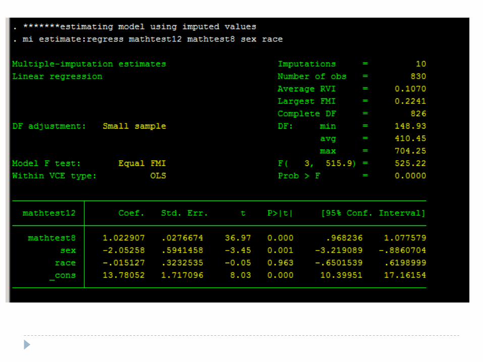
*******estimating model using imputed values
mi estimate:regress mathtest12 mathtest8 sex race


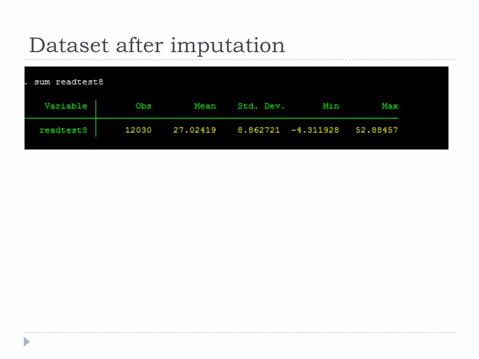
Dataset after imputation

Notes and help with mi in stata
LOTS of options
Can specify exactly how you want imputed
Can specify the model appropriately (ex. Using svy command)
mi impute mvn (multivariate normal regression) also useful
Help mi is useful
Also, UCLA has great website about ice and mi
General Tips
Try a few methods: often if result in similar estimates, can
put as a footnote to support method
Some don‟t impute dependent variable
But would still use to impute independent variables

References
Allison, Paul D. 2001. Missing Data. Sage University Papers
Series on Quantitative Applications in the Social Sciences.
Thousand Oaks: Sage.
Enders, Craig. 2010. Applied Missing Data Analysis.
Guilford Press: New York.
Little, Roderick J., Donald Rubin. 2002. Statistical Analysis
with Missing Data. John Wiley & Sons, Inc: Hoboken.
Schafer, Joseph L., John W. Graham. 2002. “Missing Data:
Our View of the State of the Art.” Psychological Methods.