
Misra - Structural Model of Sales Force Compensation
47
Quant Mark Econ (2011) 9:211–257 DOI 10.1007/s11129-011-9096-1 A structural model of sales-force compensation dynamics: Estimation and field implementation Sanjog Misra · Harikesh S. Nair Received: 6 September 2009 / Accepted: 3 February 2011 / Published online: 12 March 2011 © Springer Science+Business Media, LLC 2011 Abstract We present an empirical framework to analyze real-world sales- force compensation schemes, and report on a multi-million dollar, multi- year project involving a large contact lens manufacturer at the US, where the model was used to improve sales-force contracts. The model is built on agency theory, and solved using numerical dynamic programming techniques. The model is flexible enough to handle quotas and bonuses, output-based commission schemes, as well as “ratcheting” of compensation based on past performance, all of which are ubiquitous in actual contracts. The model ex- plicitly incorporates the dynamics induced by these aspects in agent behavior. We apply the model to a rich dataset that comprises the complete details of sales and compensation plans for the firm’s US sales-force. We use the model to evaluate profit-improving, theoretically-preferred changes to the extant compensation scheme. These recommendations were then implemented at the focal firm. Agent behavior and output under the new compensation plan is found to change as predicted. The new plan resulted in a 9% improvement in overall revenues, which translates to about $12 million incremental revenues annually, indicating the success of the field-implementation. The results bear out the face validity of dynamic agency theory for real-world compensation design. More generally, our results fit into a growing literature that illustrates that dynamic programming-based solutions, when combined with structural S. Misra Simon School of Business Administration, University of Rochester, Rochester, NY, USA e-mail: [email protected] H. S. Nair (B ) Graduate School of Business, Stanford University, Stanford, CA, USA e-mail: [email protected]
-
Upload
madminarch -
Category
Documents
-
view
220 -
download
0
description
Use dynamic programming to increase sales compensation.
Transcript of Misra - Structural Model of Sales Force Compensation

Quant Mark Econ (2011) 9:211–257DOI 10.1007/s11129-011-9096-1
A structural model of sales-force compensationdynamics: Estimation and field implementation
Sanjog Misra · Harikesh S. Nair
Received: 6 September 2009 / Accepted: 3 February 2011 / Published online: 12 March 2011© Springer Science+Business Media, LLC 2011
Abstract We present an empirical framework to analyze real-world sales-force compensation schemes, and report on a multi-million dollar, multi-year project involving a large contact lens manufacturer at the US, wherethe model was used to improve sales-force contracts. The model is built onagency theory, and solved using numerical dynamic programming techniques.The model is flexible enough to handle quotas and bonuses, output-basedcommission schemes, as well as “ratcheting” of compensation based on pastperformance, all of which are ubiquitous in actual contracts. The model ex-plicitly incorporates the dynamics induced by these aspects in agent behavior.We apply the model to a rich dataset that comprises the complete details ofsales and compensation plans for the firm’s US sales-force. We use the modelto evaluate profit-improving, theoretically-preferred changes to the extantcompensation scheme. These recommendations were then implemented at thefocal firm. Agent behavior and output under the new compensation plan isfound to change as predicted. The new plan resulted in a 9% improvement inoverall revenues, which translates to about $12 million incremental revenuesannually, indicating the success of the field-implementation. The results bearout the face validity of dynamic agency theory for real-world compensationdesign. More generally, our results fit into a growing literature that illustratesthat dynamic programming-based solutions, when combined with structural
S. MisraSimon School of Business Administration,University of Rochester, Rochester, NY, USAe-mail: [email protected]
H. S. Nair (B)Graduate School of Business,Stanford University, Stanford, CA, USAe-mail: [email protected]

212 S. Misra, H. S. Nair
empirical specifications of behavior, can help significantly improve marketingdecision-making, and firms’ profitability.
1 Introduction
Personal selling via sales-forces is an important part of the economy. In theUS, nearly 12% of the total workforce is employed in full-time sales occu-pations (Zoltners et al. 2001). In a review of sales-force practice, Albers andMantrala (2008) note,“Dartnell’s 30th Sales-force Compensation Survey: 1998–1999 reports the average company spends 10% and some industries spend asmuch as 40% of their total sales revenues on sales-force costs.” In total, the USeconomy is estimated to spend $800 billion on sales-forces, almost three timesthe amount spent on advertising in 2006 (Zoltners et al. 2008). The academicliterature has recognized this practitioner interest, and the design of plans tocompensate sales-forces is now one of the most visible and successful sales-forces applications of agency theory in real-world business settings (Mantralaet al. 1994). Surprisingly however, the richness of the theory (reviewed later),contrasts sharply with the sparsity of empirical work on the topic, stemmingpartly from the lack of detailed data on agent’s compensation and sales. Theneed for more empirical work is accentuated by the importance of accountingfor several important features of real-world compensation schemes in eval-uating and optimizing sales-force performance. Actual schemes in practicetend to be discrete and kinked, featuring quotas, bonuses and ceilings. Ina survey of Fortune 500 firms, Joseph and Kalwani (1992) report that 95%of compensation schemes they survey had some combination of quotas andcommissions, or both. These aspects complicate the analysis of contracts bygenerating dynamics in the actions of agents. A proper accounting of thesedynamics then becomes critical to the evaluation and improvement of thesales-force scheme.
The goals of this paper are two fold. First, we present a framework thatcan help evaluate the dynamic effects of compensation contracts on sales-agent output. Our approach is to develop a dynamic structural model ofagent behavior which we use, along with compensation and sales data, toestimate structural primitives underlying agent behavior. We discuss how thevariation induced by the dynamics, in combination with rich data on actualcompensation are useful in helping us learn about these primitives. Our secondgoal is to demonstrate how the model can be used to improve extant compen-sation schemes, and to cast empirical light on how compensation plans affectoutput. We demonstrate how the structural model may be used to simulateagent behavior and firms’ outcomes to uncover potentially better sales-forceplans, and to assist in plan design. Our framework can handle the rich varietyin quotas, bonuses and commissions schemes observed in practice, and canhelp decision-makers improve these plans. We present an application to thestudying the sales-force contracts of a Fortune 500 contact lens manufacturer,and report on a multi-million dollar, multi-year collaboration, as part of which

A structural model of sales-force compensation dynamics 213
the recommendations based on the model were implemented at the firm. Therecommendations involved changes to the nature and slope of output basedincentives, and resulted in a new sales-force plan at the firm starting January2009. Under the new plan, revenues to the firm increased by about $12 millionincremental per year (a 9% improvement overall), indicating the success ofthe field implementation.1 Agent behavior and the distribution of output isalso found to change as predicted by the model. We interpret these resultsas reinforcing the practical value of structural agency-theoretic models forcompensation design in real-world settings. We believe our study is one ofthe first to demonstrate the external validity of dynamic structural modelsfor improving marketing decision-making via direct field interventions. Theresults fit into a new literature that has illustrated the value of structuralmodels, more generally, for firm’s decisions (e.g. Mantrala et al. 2006; Choand Rust 2008).
The compensation plan in our data features a straight salary paid out irre-spective of effort, as well as a marginal compensation on any sales generatedabove a “quota”, and below a “ceiling”. Such quotas are ubiquitous in sales-force compensation and have been justified in the theory literature as a trade-off between the optimal provision of incentives versus the cost of implementingmore complicated schemes (Raju and Srinivasan 1996), or as optimal underspecific assumptions on agent preferences and the distribution of demand(Oyer 2000). Ceilings or caps on compensation have been rationalized as aresponse to demand uncertainty on the part of the firm. To the extent thatcompensation should reflect effort, a ceiling may help the firm hedge againstthe payout of “windfall” compensation to agents for sales that were unrelatedto effort.
While quotas are advantageous, they can also generate inefficiencies due theincentives of agents to time the allocation of effort. For instance, in a “salary +commission” scheme such as ours, sales-agents who achieve the quota requiredfor earning the commission in the current compensation cycle may have aperverse incentive to postpone additional effort to the future. Essentially, themarginal effort expended has higher marginal benefit when postponed, as itcontributes to attaining the quota in the next compensation cycle. Similardistortions arise if agents perceive they have no hope of beating quota ina cycle. In some settings, it is possible that such intertemporal reallocationof effort or “gaming” may negate the effort-inducing benefits from utilizingoutput-based compensation schemes. Similarly, ceilings have the obvious dis-advantage of destroying the desirable convexity of the plan (e.g., Basu et al.1985), thereby reducing the incentive to expend effort at high levels of output.A priori therefore, the elimination or enhancement of quotas or ceilings in aplan can either beneficial or detrimental to the firm. As this is an empirical
1These numbers may be viewed conservatively as a lower bound on the effect of the new plan dueto the recession in 2009–2010.

214 S. Misra, H. S. Nair
question, one of the questions we address is to empirically evaluate whetherthe profitability of the firm may be improved by changes to the compensationplan along these dimensions. A second question is whether reducing quotasand eliminating ceilings altogether may be better. A third question is how thesechanges may be implemented taking into account organizational and culture-based constraints faced by the firm. Together, these aspects serve to illustratethe economic and managerial implications of the framework. We focus onthese aspects specifically as they are features of the plan in our data, but thereader should note that the proposed framework is flexible enough to considerother changes to the compensation plan as well, including the introduction ofbonuses and the provision of other nonlinear, output-dependent commissionschemes.2
The main challenge in the analysis arises from the need to account forthe dynamics in agents’ actions induced by the shape of the compensationschedule. The source of the dynamics is the inherent nonlinearity of theplan. Quotas and ceilings generate curvature in the relationship betweencompensation and output. The curvature generates an incentive for effort-bunching: more is gained by the agent by expending a large effort in onemonth, than by spreading the same effort across many months. This in turnimplies that a forward-looking perspective drives agent’s effort allocationdecisions. A second dynamic arises because of a common practice termed“ratcheting” whereby quotas for future periods are updated according to theagent’s currently observed performance. Such ratcheting has been documentedin several real world compensation schemes (e.g. Weitzman 1980; Leone et al.2004), and is also a feature of the plan used by the firm in our empiricalapplication. Ratcheting implies that the agent’s current effort has an effect onhis payoffs in future quarters, thereby making his effort allocation problemdynamic. Ratcheting can help the firm fine-tune quotas to the agent’s trueproductivity or territory potential; but can result in harmful distortions tobehavior if forward-looking agents shade current effort in order to induce fa-vorable, future quotas. A careful consideration of these dynamics are essentialto the estimation of the agent’s preferences, and the simulation of his behaviorunder alternative compensation plans.
Estimation of the model is complicated by the fact that effort is unobserved.This is endemic to empirical analysis of all moral-hazard problems. It is ofparticular relevance to structural work, as the inference of the primitivesindexing the model from observed data relies on a credible backing out ofhow the agent expended effort when facing differing scenarios. We introducea methodology that exploits the richness of our data, an informative structure,and recent advances in estimation methods to facilitate the identification ofthis latent construct. In particular, following the intuition in Copeland andMonnett (2009), we describe how intertemporal linkages helps identify effort
2Solving for the optimal plan is outside of the scope of the current analysis, and is an important,but methodologically challenging, direction for future research.

A structural model of sales-force compensation dynamics 215
from sales data in sales-force compensation settings. Our strategy essentiallyinvolves using the dynamics induced by the nonlinearity and the ratcheting inthe contract for identification of hidden actions. We model agents as maximiz-ing intertemporal utility, conditional on the current compensation scheme, andtheir expectations about the process by which quotas would be updated basedon their chosen actions. Our empirical approach is to estimate, in a first stage,the structural parameters involving the sales person’s utility function. Wethen simulate, in a second stage, his behavior given a changed compensationprofile. The estimator for the 1st stage of our empirical strategy is based onthe recent literature on two-step estimation of dynamic decisions (Hotz andMiller 1993; Bajari et al. 2007). Our approach is to semiparametrically estimateagent-specific policy functions, and use these, along with the conditions for theoptimally of the observed actions, to estimate the structural parameters. Wediscuss how an individual rationality constraint as well as the assumption ofagent optimality identifies agent preferences. We use our estimates to generatethe empirical distribution of agent preferences, which we use to simulate thebehavior of the agent-pool under counterfactual compensation profiles.
A practical concern with the use of two step estimators has been the pres-ence of unobserved serially correlated state variables which prevent consistentnonparametric estimation of first-stage policy functions and transitions. Inparticular, this ruled out models with persistent unobserved heterogeneity(though see Arcidiacono and Miller 2008 for a recent approach that handlesdiscrete unobserved heterogeneity). We are able to address this problem dueto the availability of panel data of relatively long cross-section and durationfor each agent, which facilitates estimation agent-by-agent. This enables anonparametric accommodation of unobserved heterogeneity analogous to theintuition proposed by Evdokimov (2009) in the context of panel data models.Given the estimates from the first stage, we evaluate agent behavior and salesunder the counterfactual by solving the agents’ dynamic programming problemnumerically.
Our descriptive analysis of the data reveals evidence that the current planmay be inefficient. In particular, we find the incentives inherent in the currentplan are too weak, and there is evidence for shirking by agents in the early partof the compensation cycle. The model predicts that reduction or elimination ofquotas, and reduction of the length of the quota cycle reduces this perverseincentive; this aspect is borne out in the realized sales from the new plan.We also find evidence that the extent of demand uncertainty may not behigh enough to warrant the ceiling imposed on incentive compensation in thecurrent plan. Indeed, in the new plan, ceilings are eliminated, and realized salessignificantly exceed the caps from the old plan, as predicted by the model.Overall, our prediction from the model is that overall sales will rise from theelimination of quotas and ceilings, which is validated by the data from thenew plan. The fact that overall quarterly sales increased suggests the old planwas inef f icient, and that gaming resulted in reduction in aggregate orders, andnot simply intertemporal substitution. The model also predicts that under thenew plan, output variation within the months of the old compensation cycle

216 S. Misra, H. S. Nair
will be eliminated, i.e. shirking in the early sales will reduce, and effort fromthe later part of the cycle will be reallocated to earlier months. The new datacorroborates these predictions. Further, the differences in sales across monthsis not statistically significant under the new plan. Overall, these results stronglyestablish the out of sample validity and statistical power of the predictions fromthe proposed model.
Our paper adds into a small empirical literature that has explored thedynamic effects of incentive schemes. Despite the preponderance of nonlinearincentive schemes in practice, the empirical literature analyzing these, andthe effect of quotas on sales-force effort in particular, has remained sparse.Part of the reason for the paucity of work has been the lack of availabilityof agent-level compensation and output data. The limited empirical work hasprimarily sought to provide descriptive evidence of the distortionary effect ofpayment schemes on outcomes (e.g. Healy 1985, in the context of executivecompensation; Asch 1990, in the context of army-recruiters; and Courty andMarschke 1997, in the context of federal job-training programs). Oyer (1998)was the first to empirically document the timing effects of quotas, by providingevidence of jumps in firms’ revenues at the end of quota-cycles that are unre-lated to demand-side factors. On the theory side, it is well known (Holmstrom1979; Lazear 1986) that nonlinear output-based contracts, in general, havethe beneficial effect of inducing agents to exert effort, even when effort isunobservable by the firm. However, surprisingly little is known about the roleof quotas in motivating agents effort.3 In the sales-force context there is a largeliterature that investigates the design and implementation of compensationplans that induce optimal levels of sales-force effort, and examines the role ofvarious factors on the nature and curvature of the optimal contract (see for e.g.Basu et al. 1985; Lal and Srinivasan 1993; Misra et al. 2005; Rao 1990). Most ofthis literature, however, has little to say about quotas (Coughlan 1993).
A related literature also seeks to empirically describe the effect of incen-tives, more broadly, on output (e.g. Chevalier and Ellison 1997; Lazear 2000;Hubbard 2003; Bandiera et al. 2005; see Pendergast 1999 for a review).We complement this literature by detecting and measuring the dynamicinefficiencies associated with compensation schemes. The descriptive evidenceon quotas are mixed. Using data from a different context, and a differentcompensation scheme, Steenburgh (2008) reports that agents facing quotas ina durable-goods company do not tend to reduce effort in response to lump-sum bonuses. In contrast, Larkin (2010) reports on the distortionary effects ofcompensation schemes on the timing and pricing of transactions in technology-markets. The differences accentuate the need for more empirical work. Our
3An alternative motivation of output-based contracts is that it may help attract and retain the bestsales-people (Lazear 1986; Godes 2003; Zenger and Lazzarini 2004). This paper abstracts awayfrom these issues since our data does not exhibit any significant turnover in the sales-force.

A structural model of sales-force compensation dynamics 217
paper is also related to the work of Ferrall and Shearer (1999), Paarschand Shearer (2000), Lee and Zenios (2007), and Jiang and Palmatier (2009),who estimate static, structural models of agent behavior, while modeling theoptimal contract choice by the firm; and to Dufflo et al. (2010) who estimatea structural labor supply model of teachers decision to work, given nonlinearfinancial incentives they engineered as part of a randomized trial. The closestpaper to ours in spirit is Copeland and Monnett (2009) who estimate a dynamicmodel to analyze the effects of nonlinear incentives on agents’ productivity insorting checks. Our institutional context, personal selling by sales-force agents,adds several aspects that warrant a different model, analysis, and empiricalstrategy from Copeland and Monnet’s context. Unlike their industry, demanduncertainty plays a key role in our setting; this generates a role for riskaversion, and a trade-off between risk and insurance in our contracts. Further,ratcheting, an important dynamic affecting agent effort in our setting, is not afeature of their compensation scheme. Ratcheting generates a dynamic acrosscompensation periods, in addition to dynamics induced within the period bythe nonlinearity.
The methods we develop here can also be used to analyze compensationissues in other business contexts. For example, Chung et al. (2010) has usedthe framework developed here to analyze the role of bonuses in a durable goodselling context. In contrast to our application, their plan has lump-sum bonusesand a progressive incentive scheme, but no ratcheting. As limited panel datais available per agent, they use the algorithm proposed by Arcidiacono andMiller (2008) to accommodate unobserved heterogeneity. More generally, ourapproach can be used to investigate the dynamics of agent behavior undermany situations where agents optimize relative to deadlines or thresholds (e.g.,cell-phone consumption in tariff plans with pre-specified allowances of freecalls: Yao et al. 2010).
Finally, our paper also adds to the theoretical literature on sales-forcecompensation by offering a computational framework in which to examinemore realistic comparative dynamics that involve arbitrarily complex anddynamic compensation plans and effort policies of agents that respond tothese dynamics. The rest of this paper is structured as follows: We beginwith a description of our data and some stylized facts. We then introduceour model followed by the estimation methodology. We then discuss resultsand predictions for an improved plan. We then discuss results from the fieldimplementation and then conclude.
2 Patterns in the data and stylized facts
In this section, we start by presenting some stylized facts of our empiricalapplication, and also provide descriptive evidence for the effect of quotas onthe timing of effort allocations by sales-agents in our data. We use the reducedform evidence and the stylized facts presented here to motivate our subsequentmodel formulation and empirical strategy.

218 S. Misra, H. S. Nair
2.1 Data and compensation scheme
Our data come from the direct selling arm of the sales-force division of alarge contact lens manufacturer in the US with significant market-share inthe focal category (we cannot reveal the name of the manufacturer due toconfidentiality reasons). Contact lenses are primarily sold via prescriptionsto consumers from certified physicians. Importantly, industry observers andcasual empiricism suggests that there is little or no seasonality in the underlyingdemand for the product. The manufacturer employs 87 sales-agents in the U.S.to advertise and sell its product directly to each physician (also referred to as a“client”), who is the source of demand origination. The data consist of recordsof direct orders made from each doctor’s office via a online ordering system,and have the advantage of tracking the timing and origin of sales precisely.Agents are assigned their own, non-overlapping, geographic territories, andare paid according to a nonlinear period-dependent compensation schedule.We note in passing that prices play an insignificant role for output since thesalesperson has no control over the pricing decision and price levels remainedfairly stable during the period for which we have data.4 As noted before, thecompensation schedule involves salaries, quotas and ceilings. Commissionsare earned on any sales exceeding quota and below the ceiling. The salaryis paid monthly, and the commission, if any, is paid out at the end of thequarter. The sales on which the output-based compensation is earned are resetevery quarter. Additionally, the quota may be updated at end of every quarterdepending on the agent’s performance (“ratcheting”). Our data includes thehistory of compensation profiles and payments for every sales-agent, andmonthly sales at the client-level for each of these sales-agents for a period ofabout 3 years (38 months).
Quarterly, kinked compensation profiles of the sort in our data are typicalof many real world compensation schemes. Consistent with the literature, ourconversations with the management at the firm revealed that the primary moti-vation for quotas and commissions is to provide “high-powered” incentives tothe sales-force for exerting effort in the absence of perfect monitoring. We alsolearned that the motivation for maintaining a “ceiling” on the compensationscheme is consistent with the “windfall” explanation mentioned in the intro-duction. The latter observation suggests that unanticipated shocks to demandare likely important in driving sales.
The firm in question has over 15,000 SKU-s (Stock Keeping Units) ofthe product. The product portfolio reflects the large diversity in patientprofiles (e.g. age, incidence of astigmatism, nearsightedness, farsightedness orpresbyopia, corneal characteristics, eye-power etc.), patient needs (e.g. daily,disposable, sports use, cleaning frequency) and contact lens characteristics (e.g.
4In other industries, agents may have control over prices (e.g. Bhardwaj 2001). In such situations,the compensation scheme may also provide incentives to agents to distort prices to “make quota”.See Larkin (2010), for empirical evidence from the enterprise resource software category.

A structural model of sales-force compensation dynamics 219
hydrogel, silicone-hydrogel, moistness, color etc.). The product portfolio ofthe firm is also characterized by significant new product introduction and lineextensions reflecting the large investments in R&D and testing in the industry.New product introductions and line extensions reflect both new innovations aswell as new usage regimens for patients uncovered by fresh trials and testing.The role of the sales-agent is primarily informative, by providing the doctorwith updated information about new products available in the product-line,and by suggesting SKU-s that would best match the needs of the patientprofiles currently faced by the doctor. While agents’ frequency of visitingdoctors is monitored by the firm, the extent to which he “sells” the productonce inside the doctor’s office cannot be monitored or contracted upon. Inaddition, while visits can be tracked, whether a face-to-face interaction with adoctor occurs during a visit in within the agent’s control (e.g., an unmotivatedagent may simply “punch in” with the receptionist, which counts as a visit,but is low on effort).5 In our application, we do not separately model thesedimensions of sales-calls, and interpret all factors by which an agent shifts adoctors’ sales as effort.
2.2 The timing of effort
We start by checking whether dynamics are an important consideration forunderstanding agents’ behavior under this contract. We start by looking in thedata to see whether there exists patterns consistent with agent’s shifting theallocation of sales within the compensation cycle in manners consistent withincentives. First, as Oyer (1998) pointed out, when incentives exist for agentsto manipulate timing, output (i.e. sales) should look lumpy over the course ofthe sales-cycle. In particular, we expect to see spikes in output when agentsare close to the end of the quarter (and most likely to be close to “makingquota”). Figure 1 plots the sales achieved by month of quarter across sales-agents. Figure 1 reveal significant increase at the end of quarters suggestingthat agents tend to increase effort as they reach closer to quota. In the absenceof seasonality, this suggests the possibility of shirking early in the quarter.
In Fig. 2, we present plots at the agent-level that suggest that agents alsotend to reduce effort within the quarter. We plot patterns in sales (normalizedby total sales across all months in the data) for four agents. The shaded regionsin Fig. 2 highlights quarters in which sales fell in the last month of the quarter,perhaps because the agent realized a very large negative shock to demandearly in the quarter and reduced effort, or because he “made quota” earlyenough, and hence decided to postpone effort to the next sales-cycle.6 We now
5The firm does not believe that sales-visits are the right measure of effort. Even though sales-callsare observed, the firm specifies compensation based on sales, not calls.6One alternative explanation for these patterns is that the spikes reflect promotions or pricechanges offered by the firm. Our extensive interactions with the management at the firm revealedthat prices were held fixed during the time-period of the data (in fact, prices are rarely changed),and no additonal promotions were offered during this period.

220 S. Misra, H. S. Nair
Fig. 1 Sales per week bymonth of quarter
Month
Sal
es
20000
30000
40000
50000
60000
1 2 3
.04
.06
.08
.1S
ales
-sha
re
3 6 9 12 15 18Month
Agent 1
0.0
2.0
4.0
6.0
8.1
Sal
es-s
hare
3 6 9 12 15 18Month
Agent 2
.04
.06
.08
.1S
ales
-sha
re
3 6 9 12 15 18Month
Agent 3
.05
.06
.07
.08
.09
.1S
ales
-sha
re
3 6 9 12 15 18Month
Agent 4
Patterns suggesting agent 'gave up'
Fig. 2 Agents reduce effort within quarters

A structural model of sales-force compensation dynamics 221
explore how these sales-patterns are related to how far the agent is from hisquarterly quota. Figure 3 shows kernel smoothed estimates of the relationshipbetween sales (y-axis) and the distance to quota (x-axis), computed across allthe sales-people for the first two months of each quarter in the data. We define
the distance to quota as (Cumulative Sales at beginning of month-quota)quota . From Fig. 3, we
see that the distance to quota has a significant influence on the sales profile.Sales (proportional to effort) tend to increase as agents get closer to quota,suggesting increasing effort allocation, but fall once the agent reaches about40% of the quota in the first 2 months, suggesting the agent anticipates hewould “make the quota” by the end of the quarter. The decline in sales asthe agent approaches quota is also consistent with the ratcheting incentive,whereby the agent reduces effort anticipating his quota may be increased inthe next cycle, if he exceeds the ceiling this quarter. To further explore theeffect of quotas, we present in Fig. 4, nonparametric plots of the % quotaattained by the end of month T − 1 versus the % quota attained by the end ofmonth T (= 2, 3), across all agents and quarters. Figure 4 suggests patterns thatare consistent with intertemporal effort allocation due to quotas. In particular,when far away from quota in month T − 1 (x ∈ 0.2,0.4), the profile is convex,suggesting a ramping up of effort. When the agent is close to quota in monthT − 1 (x ∈ 0.5,0.8), the profile is concave suggesting a reduction in the rateof effort allocation. Finally, Fig. 4 also shows that most agents do not achieve
Fig. 3 Sales vs distance to quota

222 S. Misra, H. S. Nair
Fig. 4 Concavity in quotaattainment within eachquarter
0.2
0.4
0.6
0.8
1.0
1.2
1.4
0.2 0.4 0.6 0.8
Per
cent
age
of Q
uota
Atta
ined
at T
Percentage of Quota Attained at T−1
sales more than 1.4 × quota, which is consistent with the effect of the ceiling(which was set to be 1.33 × quota by the firm during the time-period of thedata).
Figure 5 presents the analogous relationship, with plots for each agent inthe data. Figure 5 shows that the concavity that we uncover is robust, and isnot driven by pooling across agents.
Finally, we now consider whether these patterns are due to alternativephenomena unrelated to the effects of compensation schemes. The two leadingexplanations are a) demand side seasonality; and b) buyer side stockpiling. Inthe remainder of this section, we discuss how the institutional features of oursetting, as well as the availability of some additional data enable us to rule outthese explanations.
A priori, seasonality is not a compelling consideration due to the fact thatthe disease condition the product treats is non-seasonal. Patient demand forthe product tends to be flat over the year. Our extensive discussions withsales-agents as well as the management at the firm suggest that stockpilingby clients (i.e. doctors) is also not a relevant consideration in this category.First, as noted before, there are a large number of SKU-s available from thefirm (about 15,000). The doctor is concerned about patient satisfaction andhealth, both of which are strongly linked to finding an exact match betweenthe patient’s needs and the right SKU from this large product set. Ex ante,the distribution of patient profiles, needs and usage characteristics arriving athis office for the coming month is uncertain. These considerations precludesstockpiling of SKU-s at the doctors office. The firm solves this supply-chainproblem by shipping the product directly to the consumer from its warehouse,

A structural model of sales-force compensation dynamics 223
Fig. 5 Concavity in quota attainment within each quarter by agent
upon receipt of an online order from the doctor made at his office during apatient appointment.
These aspects are also borne out in the data. To check for seasonality, weexploit some limited additional information available to us on the numberof sales-calls made by each agent at each client every month. This “call”information is available for the last 18 months of the data. The sales-call isnot a decision variable for the agent as neither the number of calls nor theallocation of calls across clients is under the control of the agent (i.e., theseare set exogenously by the firm). To test for seasonality, we use the behaviorof doctors when exposed to zero calls. We find that the sales generatedacross months with no calls are not statistically significantly different fromone another, implying no seasonality. Additionally, regressions (available onrequest) of sales on lagged sales indicate that after controlling for currentcalls, lagged sales, as well as functions of ordering history are not significant

224 S. Misra, H. S. Nair
in explaining doctor’s current orders. This is inconsistent with the stockpilingstory. Finally, a strong test that incentives drive these patterns is providedby the data from the new plan implemented at the firm. Under the newplan, incentives for sales-agents to time effort across months of the quarterare eliminated. Hence, the monthly differences should be eliminated if onlyincentives, and not buyer-side seasonality or intertemporal substitution, arethe source of the time variation. This is indeed the case: sales generation underthe new plan is found to be flat across months (please see Section 6.1.1).
Taken together, these results suggest that seasonality and buyer intertempo-ral substitution are not significant considerations for these data. These featuresarise from the specifics of our empirical setting. We anticipate that boththese aspects are likely to be important in other situations, for instance, thoseinvolving durable-good selling (e.g. Chung et al. 2010), where intertemporalsubstitution is well known to be significant, or in B2B situations where thebuyers are large firms, for which quarterly financial deadlines are knownto be an important source of buyer-side seasonality in orders (Larkin 2010;Oyer 1998). Taken together, the above descriptive evidence also point tothe existence of significant effects of the compensation scheme on agent’sintertemporal effort allocations in these data, and motivates the dynamicsincorporated into the model of agent effort.
2.2.1 Discussion
Our above discussion highlights three facts regarding salesperson effort: (i)Salespeople are forward looking in that they allocate current effort in antic-ipation of future rewards; (ii) they act in response to their current quartercompensation environment by increasing and reducing effort relative to theirquarter goals; and, (iii) salespeople take into account the impact of theircurrent actions on subsequent changes in future firm compensation policies.These facts will play key roles in the development of our formal model ofdynamic effort allocation. We discuss this next.
3 A model of dynamic effort allocation
We consider the intertemporal effort allocation of an agent facing a period-dependent, nonlinear compensation scheme. The compensation scheme in-volves a salary, αt, paid in month t, as well as a commission on sales, βt.The compensation scheme is period-dependent in the sense that it specifiesthat sales on which the commission is accrued is reset every N months. Thecompensation scheme is nonlinear in the sense that the commission βt maydepend discontinuously on the extent to which his total sales over the sales-cycle, Qt, exceeds a quota, at, or falls below a ceiling b t. The extent to whichthe ceiling is higher than the quota determines the range of sales over whichthe agent is paid the marginal compensation. While our framework is generalenough to accommodate compensation schemes where {αt, βt, at, b t} change

A structural model of sales-force compensation dynamics 225
over time, our empirical application has the feature that the salary, α and thecommission-rate, β are time-invariant, and the ceiling b t is a known deter-ministic function of the quota at. We develop the model in the context of thissimpler compensation plan. The choice of the structure of the incentive schemeby the firm is determined by reasons outside of our model. Our approach willbe to solve for the agent’s effort policy taking the firm’s compensation policyas given, and to use the model to simulate agent-effort for counterfactualcompensation profiles. Let It denote the months since the beginning of thesales-cycle, and let qt denote the agent’s sales in month t. Further, let χt be anindicator for whether the agent stays with the firm. χt = 0 indicates the agenthas left the focal company and is pursuing his outside option.7 The total sales,Qt, the current quota, at, the months since the beginning of the cycle It, andhis employment status χt are the state variables for the agent’s problem. Wecollect these in a vector st = {Qt, at, It, χt}, and collect the observed parametersof his compensation scheme in a vector � = {α, β} .
3.1 Actions
At the beginning of each period, the agent observes his state, and chooses toexert effort et. Based on his effort, sales qt are realized at the end of the period.We assume that the sales production function satisfies three conditions.
1. Current sales is a strictly increasing function of current effort.2. Current sales are affected by the state variables only through their effect
on the agent’s effort.3. Unobservable (to the agent) shocks to sales are additively separable from
the effect of effort.
Condition 1 is a standard restriction that more effort result in more sales.Monotonicity of the sales function in effort enables inversion of the effortpolicy function from observed sales data. Condition 2 implies that the quota,cumulative sales or months of the quarter do not have a direct effect on sales,over and above their effect on the agent’s effort. As is discussed in more detailbelow, this “exclusion” restriction is facilitates semiparametric identificationof effort from sales data. Condition 2 rules out reputation effects for the agent(the fact that an agent has achieved high sales in the quarter does not makehim more likely to achieve higher sales today); and also rules out direct end-of-the-quarter effects on sales (we find support for these restrictions in ourdata). Condition 3 is a standard econometric assumption. Based on the above,we consider sales-functions of the form,
qt = g (et; z, μ) + εt (1)
7We assume that once the agent leaves the firm, he cannot be hired back (i.e. χt = 0 is an absorbingstate).

226 S. Misra, H. S. Nair
where, g (.) is the sales production function, such that ∂g(e;μ)
∂e > 0, μ is avector of parameters indexing g (.); z is a vector of observed factors (such asthe number and type of clients in an agent’s sales-territory) that affects hisdemand; and εt is a mean-zero agent and month specific shock to demandthat is realized at the end of the period, which is unobserved by the agent atthe time of making his effort decision. We assume that εt is distributed i.i.d.over agents and time-periods with distribution Gε (.), to the estimated fromthe data. εt serves as the econometric error term in our empirical model (wepresent our econometric assumptions in detail in Section 4.1). In our empiricalwork, we will consider specifications in which the all the parameters indexingthe production function g (.) are heterogeneous across agents. For now, wesuppress the subscript “i” for agent for expositional clarity.
3.2 Per-period utility
The agents’ utility is derived from his compensation, which is determined bythe incentive scheme. We write the agent’s monthly wealth from the firm as,Wt = W (st, et, εt; μ, �). We model his utility each month as derived from thewealth from the firm minus the cost of exerting effort. We denote the costfunction as C (et; d), where d is a parameter to be estimated. We assume thatagents are risk-averse, and that conditional on χt = 1, their per-period utilityfunction is,
ut = u (Qt, at, It, χt = 1) = E [Wt] − r var [Wt] − C (et; d) (2)
Here, r is a parameter indexing the agent’s risk aversion, and the expectationand variance of wealth is taken with respect to the demand shocks, εt. Thespecification in Eq. 2 is attractive since it can be regarded as a second orderapproximation to an arbitrary utility function.8 We now discuss the transitionof the state variables that generate the dynamics in the agent’s effort allocationproblem. The payoff from leaving the focal firm and pursuing the outsideoption is normalized to zero,
ut = u (Qt, at, It, χt = 0) = 0 (3)
3.3 State transitions
There are two sources of dynamics in the model. The nonlinearity in thecompensation scheme generates a dynamic into the agent’s problem becausereducing current effort increases the chance to cross, say, the quota thresholdtomorrow. A second dynamic is introduced since the agent’s current effort
8In case of the standard linear compensation plan, exponential CARA utilities and normal errorsthis specification corresponds to an exact representation of the agent’s certainty equivalent utility.

A structural model of sales-force compensation dynamics 227
also affects the probability that his compensation structure is updated in thefuture. Hence, in allocating his effort each period, the agent also needs totake into account how current actions affect his expected future compensationstructure. These aspects are embedded in the transitions of the state variablesin the model. In the remainder of this section, we discuss these transitions.Subsequently, we present the value functions that encapsulate the optimalintertemporal decisions of the agent.
The first state variable, total sales, is augmented by the realized sales eachmonth, except at the end of the quarter, when the agent begins with a freshsales schedule, i.e.,
Qt+1 ={
Qt + qt i f It < N0 i f It = N
(4)
We assume that the agent has rational expectations about the transition of hisquota, at. We use the observed empirical data on the evolution the agent’squotas to obtain the transition density of quotas over time. We estimate thefollowing transition function that relates the updated quota to the currentquota, as well as the performance of the agent relative to that quota in thecurrent quarter,
at+1 ={
at i f It < N∑Kk=1 θk (at, Qt + qt) + vt+1 i f It = N
(5)
In Eq. 5 above, we allow the new quota to depend flexibly on at and Qt +qt, via a K-order polynomial basis indexed by parameters, θk. We use thisflexible polynomial to capture in a reduced-form way, the manager’s policyfor updating agents’ quotas. The term vt+1 is an i.i.d. random variate which isunobserved by the agent in month t. The distribution of vt+1 is denoted Gv (.),and will be estimated from the data. Allowing for vt+1 in the transition equationenables us to introduce uncertainty into the agent’s problem. In our empiricalwork, we extensively test different specifications for the ratcheting policy, andprovide evidence that the associated errors vt+1 are not serially correlated inthe specifications we use. Lack of persistence in vt+1 implies that all sources oftime-dependence in the agent’s quota updating have been captured, and thatthe remaining variation is white noise.9
The transition of the third state variable, months since the beginning of thequarter, is deterministic,
It+1 ={
It + 1 i f It < N1 i f It = N
(6)
9We also reject correlation of vt+1 across agents, as well as correlation of vt+1 with the demandshocks (εt) across agents. This rules out a story where subjective quota updating is used as amechanism to filter out common shocks.

228 S. Misra, H. S. Nair
Finally, the agent’s employment status in (t + 1), depends on whether hedecides to leave the firm in period t. The employment state tomorrow is thus acontrol variable for the agent today, and is described below.
3.4 Optimal actions
Given the above state-transitions, we can write the agent’s problem as choos-ing effort to maximize the present-discounted value of utility each period,where future utilities are discounted by the factor, ρ. We collect all theparameters describing the agent’s preferences and transitions in a vector� = {
μ, d, r,Gε (.) ,Gv (.) , θk,k=1,..,K}. In month It < N, the agent’s present-
discounted utility under the optimal effort policy can be represented by a valuefunction that satisfies the following Bellman equation,
V (Qt, at, It, χt; �, �)
= maxχt+1∈(0,1),e>0
⎧⎪⎨⎪⎩
u (Qt, at, It, χt, e; �, �)
+ρ
∫ε
V(Qt+1 = Q(Qt,q(εt,e)),at+1 =at,It+1,χt+1;�,�) f (εt) dεt
⎫⎪⎬⎪⎭
(7)
The value in period It + 1 is stochastic from period It’s perspective because theeffort in period It is decided prior to the realization of εt, which introduces un-certainty into the cumulative sales attainable next period. Hence, the Bellmanequation involves an expectation of the (It + 1)—period value function againstthe distribution of εt, evaluated at the states tomorrow. Similarly, the Bellmanequation determining effort in the last period of the sales-cycle is,
V (Qt, at, N, χt; �, �)
= maxχt+1∈(0,1),e>0
⎧⎪⎪⎪⎨⎪⎪⎪⎩
u (Qt, at, N, χt, e; �, �)
+ρ
∫v
∫ε
V(Qt+1 =0, at+1 =a (Qt, q (εt,e) ,at,vt+1),1, χt+1;�,�)
× f (εt) φ (vt+1) dεtdvt+1
⎫⎪⎪⎪⎬⎪⎪⎪⎭(8)
At the end of the sales-cycle, the cumulative sales is reset and the quotais updated. The value in the beginning of the next cycle is again stochasticfrom the current perspective on account of the uncertainty introduced into theratcheted future quota by the demand shock, εt, and the quota-shock, vt+1.Hence, the Bellman equation in Eq. 8 involves an expectation of the 1st periodvalue function against the distribution of both εt and vt+1.

A structural model of sales-force compensation dynamics 229
Conditional on staying with the firm, the optimal effort in period t, et =e (st; �, �) maximizes the value function,
e (st; �, �) = arg maxe>0
{V (st; �, �)} (9)
The agent stays with the firm if the value from employment is positive, i.e.,
χt+1 = 1 if maxe>0
{V (st; �, �)} � 0
Given the structure of the agent’s payoffs and transitions, it is not possible tosolve for the value function analytically. We solve for the optimal effort policynumerically via modified policy iteration. The state-space for the problem isdiscrete-continuous, of dimension R
2 × (N + 1). The two continuous dimen-sions (Qt and at) are discretized, and the value function is approximated overthis grid for each discrete value of N and employment status. One iterationof the solution took 120 s on a standard Pentium PC. Further computationaldetails of the algorithm are provided in the Appendix. We now present theapproach for the estimation of the model parameters.
4 Empirical strategy and estimation
Our empirical strategy is motivated by the intended use of the model, which isto obtain a relative evaluation of the outcomes for the firm under a changedcompensation scheme. This requires a method to simulate the outcomes forthe firm under new compensation schemes. Consider a new compensation plan℘ (q (e) ; �), where � indexes the parameters governing the features of thenew plan (e.g. a revised salary, bonus, commission rate, quota etc.), and q (.) issales in dollars.10 The firm’s present discounted payoffs under ℘ (q (e) ; �) are,
�℘ =∫ ∫ ∞∑
τ=0
ρτ
[q
(e℘
) − ℘(q
(e℘
)) − cp
q(e℘
)]dF (μ, r, d) dGε (ετ ) (10)
where(e℘
)is the effort policy expended by the agent when faced with
compensation policy ℘ (q (e)),
e℘ = arg maxe>0
V (s; e| {μ, r, d} , ℘ (.))
p is the unit price per contact-lens, and c is the marginal cost of manufacturingq(e℘)
p lenses (the marginal cost of manufacturing a lens is small, of the order of
10Implilcity, � can be a function of the agent’s characteristics, � ≡ � (μ, r, d,Gε (.)). For example,a counterfactual scheme could be characterized by a fixed salary and a commission specific to eachagent. In this contract, the optimal salary and commision rate would be a function of the agent’spreferences. We suppress the dependence of � on these features for notational simplicity.

230 S. Misra, H. S. Nair
25–50 cents). In Eq. 10, F (μ, r, d) is the joint CDF across agents in the firm ofdemand parameters, risk aversion and the cost of effort. Our approach will beto use the model to simulate effort and sales under the counterfactual plans,conditioning on estimates of F (μ, r, d) and Gε (ετ ).11 A comparison of currentpolicy quantities {�∗, q∗, e∗} to the counterfactual then facilitates a relativeevaluation of the current plan to other potentially, better possibilities. The keyobject of econometric inference is thus the joint distribution of preferences,F (μ, r, d) and of demand uncertainty, Gε (ετ ). In the section below, we discussa methodology that delivers estimates of these distributions.
Our discussion below comprises two steps. In step 1, we discuss how we usethe observed data on sales and compensation plans across agents to estimatethe parameters of the agents’ preferences, as well as the functions linkingsales to effort. In step 2, we discuss how we use these parameters, along withour dynamic programming (henceforth DP) solution to simulate the agent’sactions under counterfactual compensation profiles. In the remainder of thissection, we first discuss our econometric assumptions, and then present detailson the specific compensation scheme in our data. Subsequently, we describethe procedure for estimation of the parameters of the model.
4.1 Econometric assumptions
The econometric assumptions on the model are motivated by the nature of thedata, as well as the intended procedure for estimation. The observed variationto be explained by the model is the correlation of sales across months withthe distance to quotas, the changes in sales when quotas change, as well as thevariation of sales across agents, which are a function of the agents’ effort. Thecomputational challenge in estimation derives from the fact that the modelimplies that each agent’s effort, and consequently, their sales, are solutions toa dynamic problem that cannot be solved analytically.
One approach to estimation would be to nest the numerical solution ofthe associated DP into the estimation procedure. This would be significantlynumerically intensive since the DP has to be repeatedly solved for each guessof the parameter vector. Instead, our estimation method builds on recentlydeveloped methods for two-stage estimation of dynamic models (e.g. Hotz
11Implicity, in Eq. 10, we assume that the distribution of demand shocks, Gε (.) stays the sameunder the counterfactual. In Eq. 10, we do not intergate against the ratcheting shocks Gv (.),because all the counterfactual contracts we consider involve no ratcheting. Consideration ofcounterfactual contracts that involve ratchting would require a model for agents’ belief formationabout quota updating under the new compensation profile, which is outside of the scope of thecurrent analysis. Future research could consider solving for the optimal quota updating policy,under the assumption that agents’ beliefs regarding ratcheting are formed rationally. See Nair(2007) for one possible approach to solving for beliefs in this fashion applied to durable goodpricing.

A structural model of sales-force compensation dynamics 231
and Miller 1993; Bajari et al. 2007, henceforth BBL), which obviates the needto solve the DP repeatedly. Under this approach, agents’ policy functions—i.e., his optimal actions expressed as a function of his state—as well as thetransition densities of the state variables are estimated semiparametrically ina first-stage; and subsequently, the parameters of the underlying model areestimated from the conditions for optimality of the chosen actions in the data.We face two difficulties in adapting this approach to our context. First, therelevant action—effort—is unobserved to the econometrician, and has to beinferred from the observed sales. This implies that we need a way to translatethe sales policy function to an “effort policy function”. Second, unobservedagent heterogeneity is likely to be significant in this context, since we expectagents to vary significantly in their productivity. The dependence of saleson quotas induced by the compensation scheme generates a form of statedependence in sales over time, which in the absence of adequate controls foragent heterogeneity generates well-known biases in the estimates of the effortpolicy. However, handling unobserved heterogeneity in the context of 2-stepHotz-Miller type estimators has been difficult to date (there has been recentprogress on this topic; please see Arcidiacono and Miller 2008).
We address both issues in our proposed method. To handle the first issue, wemake a parametric assumption about the sales-production function. We discussbelow why a nonparametric solution is not possible. We are able to handlethe second issue due to the availability of sales-information at the agent-levelof unusually large cross-section and duration, which enables us to estimateagent-specific policy functions, and to accommodate nonparametrically theheterogeneity across agents. We discuss the specific assumptions in more detailbelow.
4.1.1 Preliminaries
The model of agent optimization presented in Section 3 implies that theoptimal effort each period is a function of only the current state st. Toimplement a two step method, we thus need to estimate nonparametricallyin a first-stage, the effort policy function, et = e (st). The effort policy functionis obtained parametrically from the sales-policy function. To see the need for aparametric assumption, recall from Section 3 that we consider sales-productionfunctions of the form,
qt = g (et (st) , z) + εt
For clarity, we suppress the variable z, as the argument below holds for eachvalue of z. Let f (st) ≡ g (et (st)).
Remark 1 If at least two observations on q are available for a given value of s,the density of f (s) and ε are separately nonparametrically identified (Li andVuong 1998).

232 S. Misra, H. S. Nair
Remark 2 Given the density of f (s), only either g (s) or e (s) can be estimatednonparametrically.
Remark 2 underscores the need for a parametric assumption on the rela-tionship between sales and effort. One option to relax this would be to obtaindirect observations on agent’s effort, via say, survey data, or monitoring. Thisof course, changes the character of the principal-agent problem between theagent and the firm. Unobservability of agent effort is the crux of the moralhazard problem in designing compensation schemes. Hence, we view this para-meterization as unavoidable in empirical models of sales-force compensation.
We now discuss how we use this assumption, along with the sales data toestimate the sale-production function. For each agent in the data, we observesales at each of J clients, for a period of T months. In our empirical applicationT is 38 (i.e., about 3 years), and J is of the order of 60–300 for each agent.The client data adds cross-sectional variation to agent-level sales which aidsestimation. To reflect this aspect of the data, we add the subscript j for clientfrom this point onward. In light of Remark 2 we assume that the productionfunction at each client j is linear in effort,
q jt = h j + et + ε jt (11)
= h j(z j
) + e (st) + ε jt (12)
The linear specification is easy to interpret: h j can be interpreted as the agent’stime-invariant intrinsic “ability” to sell to client j, which is shifted by clientcharacteristics z j. We now let h j ≡ μ′z j, and let e (st) = λ′ϑ (st), where γ is aR × 1 vector of parameters indexing a flexible polynomial basis approximationto the monthly effort policy function. Then, the effort policy function satisfies,
q jt = μ′z j + λ′ϑ (st) + ε jt (13)
We assume that ε jt is distributed i.i.d. across clients. We can then obtainthe demand parameters and the effort policy function parameters from thefollowing minimization routine,
minμ,λ
∥∥q jt − (μ′z j + λ′ϑ (st)
)∥∥ (14)
As a by product, we also obtain the effort policy function for the month t foreach client as,
et = λ′ϑ (st) (15)
and the time-specific error distribution,
εt =∑
j
(q jt −
(μ′z j + λ′ϑ (st)
))(16)

A structural model of sales-force compensation dynamics 233
which is then used to estimate the empirical distribution of εt for eachagent.12 This distribution is an input to solving the dynamic programmingproblem associated with solution of the model for each agent. We sample withreplacement from the estimated empirical distribution for this purpose.
Finally, at the end of this step, we can recover the predicted overall sales forthe agent which determines the agent’s overall compensation. Summing Eq. 13across clients, the overall sales in month t is,
qt =J∑j
qjt = h + Jet + εt (17)
where, h = ∑Jj=1 μ′z j, and εt = ∑J
j=1 εjt. The total effort expended by a sales-agent across all clients in period t is thus Jet, which affects per-period payoffsthrough Eq. 2.
Intuition for estimation of ef fort: Intuitively, we can think of identification ofthe effort policy by casting the estimator in Eq. 13 in two steps,
• Step 1: Estimate time-period fixed effects �t as, q jt = μ′z j + �t + ε jt• Step 2: Project �t on a flexible function of the state variables as �t =
λ′ϑ (st)
The client-level data facilitates the estimation of time-period specific fixedeffects in Step 1. Equation 13 combines steps 1 & 2 into one procedure. Wediscuss the identification of the model in further detail below.
4.2 Compensation scheme
We now discuss the specifics of the compensation scheme in our dataset,and derive the expression for the monthly expected wealth for the agentgiven the above econometric assumptions. The agent’s payout under the planis determined based on his quarter-specific performance. Thus, N = 3, andcumulative sales, which affect the payout, are reset at the end of each quarter.The monthly salary α is paid out to the agent irrespective of his sales. If hiscurrent cumulative sales are above quota, the agent receives a percentage of afixed amount β as commission. The percentage is determined as the proportionof sales above at, and below a maximum ceiling of b t, that the agent achieves inthe quarter. Beyond b t, the agent receives no commission. For the firm in our
12Alternatively, one could assume a parameteric density for ε and use maximum likelihoodmethods. The advantage of our semiparametric approach is that we avoid the possibility ofextreme draws inherent in parametric densities and the pitfalls that go along with such draws.

234 S. Misra, H. S. Nair
Fig. 6 Compensation scheme
empirical application, β = $5, 000 per quarter, and the ceiling was always set33% above the quota, i.e., b t = 4
3 at. Figure 6 depicts the compensation scheme.We can write the agent’s wealth, W (st, et, εt; μ, �) in Eq. 2 as,
W (st, et, εt; μ, �) = α + β
[(Qt+qt−at
b t−at
)I (at ≤ Qt + qt ≤ b t)
+I (Qt + qt > b t)
]I (It = N) (18)
Thus, at the end of each sales-cycle, the agent receives the salary α, as well as an
incentive component, β × {(
Qt+qt−atb t−at
)I (at ≤ Qt + qt ≤ b t) + I (Qt + qt > b t)},
on any sales in excess of quota. If it is not the end of the quarter, I (It = N) = 0,and only the salary is received.
Finally, we assume that the cost function in Eq. 2, C (e), is quadratic in effort,i.e. C (et) = de2
t2 , where d is a parameter to be estimated. The discount factor ρ
is fixed at 0.98.
4.3 Estimation procedure
We now present the steps for estimation of the model parameters. The estima-tion consists of two steps, the first for a set of “auxiliary” parameters, and thesecond for a set of “dynamic parameters.” We discuss these in sequence below.
4.3.1 Step 1: semiparametric estimation of policy function and state transitions
The goals of the first step are two-fold. First, we estimate the demand para-meters μ, as well as the distribution of demand shocks Gε (ετ ) for each agent.

A structural model of sales-force compensation dynamics 235
Second, we estimate an effort policy function, as well as transitions of the statevariables for each agent. We use both set of objects to estimate F (μ, r, d) instep 2.
The effort policy function is related to observed sales via Eq. 13. Thedemand parameters and the demand shock distribution are obtained as by-products of estimating Eq. 13. We estimate the effort policy agent-by-agent.For each agent, data are pooled across the agent’s clients, and Eq. 13 estimatedvia least squares. An advantage of this approach is that we are able to handleheterogeneity across agents nonparametrically.
The next step is to estimate the parameters (θk,Gv (.)) describing thetransition of the agent’s quotas in Eq. 5. This is a series estimator which weestimate via nonlinear least squares. Since quotas vary only at the quarter-level, we do not estimate the quota transitions agent-by-agent. Instead, we poolthe data across agents to estimate the quota transition function allowing foragent fixed-effects. The distribution of ratcheting shocks, Gv (.), are estimatedsemiparametrically from the residuals from this regression.
The law of motion of the other state variables (month-of-the-quarter) doesnot have to be estimated since it does not involve any unknown parameters.This concludes step 1. Since we have estimated μ agent by agent, we canconstruct its marginal CDF (F (μ)) using a simple estimator,
F (μ) = 1N
N∑i=1
I (μi ≤ μ) . (19)
The only remaining object to be estimated is the conditional distribution ofthe risk aversion, r, and the cost parameter, d,F (r, d|μ). Step 2 below deliversestimates of F (r, d|μ).
4.3.2 Step 2: estimation of F (r, d|μ)
We estimate the “dynamic” parameters r and d using the methods proposed inBBL for the case of continuous controls. The BBL estimator is a minimumdistance estimator that finds parameters which minimize a set of momentinequality conditions. We propose to estimate the parameters by imposingtwo moment conditions that arise naturally in the class of principal-agentproblems. In particular, let s0 be an initial state for an agent, (r∗, d∗) be thetrue parameters, and e∗ the optimal effort policy at the true parameters. Then,(r∗, d∗) must satisfy,
1. Individual Rationality (IR): V (s0; e∗, r∗, d∗) ≥ 02. Incentive Compatibility (IC): V (s0; e∗, r∗, d∗) ≥ V
(s0; e′, r∗, d∗)
where V (s0; e∗, r∗, d∗) is the value function corresponding to the optimal policye∗, and V
(s0; e′, θ∗) is the present discounted utility corresponding to any other
feasible policy, e′ = e∗. The IR constraint says that the agent should at least

236 S. Misra, H. S. Nair
be as better off working with the firm, as leaving the firm and pursuing hisoutside option. The IC constraint says that the agent should obtain higherutility in present discounted terms under the optimal effort policy, compared toany other feasible effort policy. Following BBL, we propose to estimate r∗, d∗by finding the set of parameters that minimize violations of these conditionsover a random sample of the state space. In what follows, we assume that theoptimal policy function e∗ = e∗ (s0) has already been estimated in step 1, and isavailable to the econometrician. Begin by defining the following quantities,
Z(s0; e∗) = [
E (W) V (W) C (e)]
(20)
θ = [1 r d
](21)
where θ are the “dynamic” parameters to be estimated, s0 is an initial state, e∗is the estimated optimal effort policy function and Z (s0; e∗) has components,
E (W) = Ee∗|s0
∞∑t=0
ρ t Eε
[W
(s, e∗ (s)
)](22)
V (W) = Ee∗|s0
∞∑t=0
ρ t Eε
[W
(s, e∗ (s)
)2 − Eε
[W
(s, e∗ (s)
)]2]
C (e) = Ee∗|s0
12
∞∑t=0
ρ te∗ (s)2 (23)
The value function based on the optimal effort policy can then be expressedas,
V(s0; e∗, θ
) = Z(s0; e∗)′
θ (24)
Similarly, for any alternative policy function(e′ = e∗) , the perturbed value
function is,
V(s0; e′, θ
) = Z(s0; e′)′
θ (25)
Define the following two moment conditions,
g1 (s0; θ) = min(V
(s0; e∗, θ
), 0
)(26)
g2(s0, e′; θ
) = min(V
(s0; e∗, θ
) − V(s0; e′, θ
), 0
)
and let g(s0, e′; θ
) = [g1 (s0; θ) g2 (s0; θ)
]′.Let H (.) be a sampling distribution over states s0 and alternative feasible
policies e′. Define an objective function,
Q (θ) =∫ [
g(s0, e′; θ
)]′�
[g
(s0, e′; θ
)]dH
(s0, e′) (27)

A structural model of sales-force compensation dynamics 237
where, � is a 2 × 2 weighting matrix. Clearly, the true parameter vector(θ = θ∗) must satisfy,
Q(θ∗) = min
θ(Q (θ)) = 0 (28)
Following BBL, we estimate θ∗ by minimizing the sample analog of Q (θ).The function is Q (θ) is obtained by averaging its evaluations over NR i.i.d.draws of s0 from a uniform distribution over the observed support of statesfor the agent. At each s0, we generate alternative feasible policies by addinga normal error term to the estimated optimal effort policy. Using these, weforward simulate the terms in Eq. 22 to evaluate the moments at each guess ofthe parameter vector. The linearity of the value functions in θ imply that wecan pre-compute Z (s0; e∗) and Z
(s0; e′) prior to parameter search, reducing
computational time. In principle, an “optimal” � that weights each of themoment conditions based on their informativeness about θ would give themost efficient estimates. However, the econometric theory for the optimal� for inequality estimators of this sort are still to be developed. Hence, inpractice, we set � equal to the identity matrix. This yields consistent but po-tentially inefficient estimates. Further computational details of our estimationprocedure are presented in the Appendix.
We perform estimation agent by agent. The main computational burdenarises from forward-simulating value functions and implementing the nonlin-ear search separately for each agent (i.e. we solve 87 separate minimizationproblems). For each, we obtain point estimates of r, d|μ. We use these toconstruct a nonparametric estimate of the CDF across agents, F (r, d|μ) as inthe earlier section.
In general, the approach above yields point estimates of the parameters.Point estimation implies that the optimizer finds no other value of θ otherthan θ∗ for which Q (θ) = 0. Point identification is facilitated by the addedimposition of the IR constraint, which imposes that the value function atevery state has be positive (or greater than a reservation value). Removingthis constraint will in general, result in set identification. A working version ofthe paper reported identified sets. We also explored sensitivity of the results tonormalizing the value of the outside option to average life-time wages for sales-agents. Our view is that adding the IR constraint is reasonable and consistentwith the spirit of principal-agent theory for this class of models. A criticaldeterminant to the point identification of the parameters is H (.). In particular,H (.) has to have large enough support over the states and alternative feasibleeffort policies to yield identification. This in turn requires that we a) pick thealternative feasible policies “intelligently”, such that they are informative ofθ ; and b) more importantly, the econometrician has access to sufficient data(i.e. state points), on which nonparametric estimates of the optimal policy areavailable, and from which s0-s can be sampled. In application, we found thatperturbations of the effort policy that were too far away from the effort policywere uninformative of the parameter vector. We use “small” perturbations(see the Appendix for precise details), which combined with the richness of

238 S. Misra, H. S. Nair
our data, yield point identification of the parameters in our context for all theagents in the data.
4.4 Discussion: identification
We now provide a more detailed discussion of identification in our model. Inparticular, we discuss how intertemporal linkages in observed sales identifiesan agent’s unobserved effort allocation over time. The first concern is thateffort has to be inferred from sales. In particular, looking at Eq. 11, we seethat sales is explained by two unobservables, the first, effort, and the second,client-specific demand shocks. How can the data sort between the effects ofeither? The key identifying assumptions are,
1. Effort is a deterministic function of only the state variables.2. Effort is not client specific—i.e., the agent allocates the same effort to each
client in a given month.
We believe the first assumption is valid since we believe we have capturedthe key relevant state variables generating the intertemporal variation in agenteffort. Further, after including a rich-enough polynomial in the state variablesin Eq. 11, we can reject serial correlation in the residuals, εjt (i.e. the remainingvariation in sales is only white noise). Assumption 1 is also consistent withour dynamic programming model which generates a deterministic policy byconstruction. We believe the second assumption is reasonable. In separateanalysis (not reported), we use limited data on the number of sales calls madeby agents to each of the clients to check the validity of this assumption. Inregressions of sales on calls, we find that the marginal effect of calls is notstatistically significantly different across client-types, suggesting that effortmore broadly, is not being tailored to each individual client.
Given these two assumptions, effort is identified by the joint distributionover time of the agent’s current sales, and the extent to which cumulativesales are below or above the quota and the ceiling. To see this, recall that theoptimal policy implies that the agent expends high effort when he is close to thequota, irrespective of month. The agent expends low effort when he has eithercrossed the ceiling in a given quarter, or when he is very far away from thequota in an early month. Under the former situation, the marginal benefit of anadditional unit of effort is higher when expended in the next quarter; the sameis true under the latter, since he has very little chance of reaching the quotain the current quarter. The model assumes that sales are strictly increasing ineffort. Hence, if we see an agent achieve high sales across clients when he isclose to the quota we conclude that effort is high. If we see low sales earlyon in the quarter, and when the quarter’s sales have crossed the ceiling, weconclude that effort is low. Our identification argument is based essentially onthe fact that dynamics induced by the contract help identification of hiddenactions. That is, the induced dynamics imply that variation in effort over timeis related to variation in the distance to quota over time (the relevant statevariable). This intuition is similar to the identification of productivity shocks in

A structural model of sales-force compensation dynamics 239
the production economics literature (see e.g. Olley and Pakes 1996; Ackerberget al. 2006). Note the significant role played by the nonlinearity of the contractas well as ratcheting in identification of effort: in particular, if the firm adopteda purely linear incentive scheme with no quota updating, that would reducethe econometrician’s ability to identify the hidden action in this manner sincethen, there is no variation over time in the shadow value of working.
A related concern is how the effect of ratcheting is identified separatelyfrom the intertemporal substitution induced by the quota structure. The dataare able to sort between these two separate dynamics in the following way.The extent of decline in the agent’s observed sales after he crossed the ceilingin any quarter informs the model about the extent of intertemporal effortallocation induced by the quota structure. However, note that in the absenceof ratcheting, effort, and hence, sales, should be strictly increasing betweenthe quota and the ceiling. Hence, the extent of decline in the agent’s observedsales after he crosses the quota, and before he attains the ceiling informs themodel about the extent to which ratcheting plays a role. Figure 7 depicts theidentification argument pictorially. The two other key parameters that areestimated in step 3 above are the cost (d) and risk aversion parameter (r) .
The cost of effort parameter is identified from the fact that sales are abovethe intercept in the first two months of the quarter. That is, if effort werecostless, it would be optimal to exert no effort in the first two months andmeet any target in the third month alone. The fact that effort is costly inducesa constraint on how much sales can be generated in any given month. This,along with the structure of the sales response function, acts as the primaryidentification mechanism for the cost of effort parameter. Finally, the riskaversion parameter is identified by the degree to which effort (sales) changesdue to changes in the variance of wealth. This variation in wealth is generatedby within-agent factors that shift demand over time that are unrelated to theagent’s distance to quota.
Fig. 7 Identification of effortfrom sales profile

240 S. Misra, H. S. Nair
5 Data and estimation results
Table 1 presents summary statistics from our data. The sales-force has 87salespeople who are about 43 years of age on average, and have been with thefirm for approximately 9 years. The firm did not significantly hire, nor have sig-nificant employee turnover in this sales-department during the time-period ofthe data.13 The average salesperson in the sales-force earns $67,632 per annumvia a fixed salary component. The annual salary ranges across the sales-forcefrom around $50,000 to about $90,000. The firm’s output-based compensationis calibrated such that, on a net basis, it pays out a maximum of $5,000 peragent per quarter, if the agent achieves 133% of their quarterly quota. On anaverage this implies that the agent has a 77–23% split between fixed salary andincentive components if they achieve all targets. Across agents-quarters in thedata, the average proportion of quarterly payout due to incentives is 16.8%(std. dev. 20.9%). In dollar terms total compensation ranges from around$55,000 to about $105,000 in the data. Agents have exclusive territories anddiffer in terms of the number of clients they have, but are balanced in terms ofthe type of clients and the total sales-calls they are required to make.
The mean quota for the sales-force is about $321,404 per quarter. The meanattained sales stands at $381,210, suggesting that agents at the firm tend totarget quarterly sales in the range in which incentives are earned. This isfurther evidenced by the fact that the range and dispersion parameters of thecumulative sales at the end of the quarter and the quota levels are also fairlyclose.
From Table 1, it appears on average that the firm adopts an asymmetricratcheting approach to quota setting. When salespeople beat quotas the av-erage increase in subsequent quarter quotas is about 10%, but on the flipside, falling short of quotas only reduces the next quarter quota by about5.5%. This is consistent with some other earlier studies (e.g. Leone et al. 2004)that document such behavior at other firms, and is also consistent with ourconversations with the firm management. Finally, the table documents thatmonthly sales average about $138,149, a fairly significant sum.
5.1 Results from estimation
We now report the results from estimation. We first discuss the results fromthe first stage, which includes estimation of the effort policy function, andthe quota transition process. Subsequently, we discuss the results from theestimation of the cost function and risk aversion parameters.
13So as to avoid concerns about learning-on-the job, and its interactions with quotas, five sales-agents, who had been with the firm for less than 2 years were dropped from the data.

A structural model of sales-force compensation dynamics 241
Table 1 Descriptive statistics of data
Variable Mean SD Min Max
Agent demographicsSalary $67,632.28 $8,585.13 $51,001.14 $88,149.78Incentive proportion at ceiling 0.23 0.02 0.28 0.8Age 43.23 10.03 27 64Tenure 9.08 8.42 2 29Number of clients 162.20 19.09 63 314
Quarter level variables (across agents)Quota $321,404 $86,112.67 $178,108.93 $721,770.14Cumulative sales (end of quarter) $381,210 $89,947.66 $171,009.11 $767,040.98Percent change in quota (when positive) 10.01% 12.48% 00.00% 92.51%Percent change in quota (when negative) −5.53% 10.15% −53.81% −00.00%
Monthly level variables (across agent-months)Monthly sales $138,149 $38,319.34 $45,581.85 $390,109.07Cumulative sales (beginning of month) $114,344 $98,594.65 $0 $652,474.25Distance to quota (beginning of month) $278,858 $121,594.2 $20,245.52 $835,361.10
Number of salespeople 87
5.1.1 Ef fort policy
The effort policy function was estimated separately for each agent usinga flexible Chebychev polynomial basis approximation. We approximate theeffort policy using the tensor product of basis functions of dimension 2 in eachof the two continuous state variables (cumulative sales and quota), allowingmonth specific intercepts, and allowing the first two basis functions to bemonth specific. We find that this specification fits the data very well. Onaverage, we are able to explain about 79% of the variation in observed sales.Figure 8 plots a histogram of the R2 values from the estimation across agents.
Fig. 8 Histogram of R2
values from first-stage effortpolicy estimation
0.55 0.6 0.65 0.7 0.75 0.8 0.85 0.9 0.950
2
4
6
8
10
R-square values
Freq
uenc
y
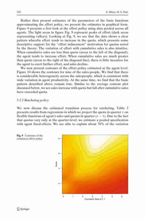
242 S. Misra, H. S. Nair
Rather then present estimates of the parameters of the basis functionsapproximating the effort policy, we present the estimates in graphical form.Figure 9 presents a first look at the effort policy using data pooled across allagents. The light areas in figure Fig. 9 represent peaks of effort (dark areasrepresenting valleys). Looking at Fig. 9, we see that the data shows a clearpattern whereby effort tends to increase in the quota, which presents somedescriptive support for the “effort inducement” motivation for quotas notedby the theory. The variation of effort with cumulative sales is also intuitive.When cumulative sales are less than quota (areas to the left of the diagonal),the agent tends to increase effort. When cumulative sales are much greaterthan quota (areas to the right of the diagonal line), there is little incentive forthe agent to exert further effort, and sales decline.
We now present contours of the effort policy estimated at the agent level.Figure 10 shows the contours for nine of the sales-people. We find that thereis considerable heterogeneity across the salespeople, which is consistent withwide variation in agent productivity. At the same time, we find that the basicpattern described above remain true. Similar to the average contour plotdiscussed below, we see sales increase with quota but fall after cumulative saleshave exceeded quota.
5.1.2 Ratcheting policy
We now discuss the estimated transition process for ratcheting. Table 2presents results from regressions in which we project the quota in quarter τ onflexible functions of agent’s sales and quotas in quarter (τ − 1). Due to the factthat quotas vary only at the quarter-level, we estimate a pooled specificationwith agent fixed-effects. We are able to explain about 78% of the variation
Fig. 9 Contours of theestimated effort policy
0 1 2 3 4 5 6
24
68
Quo
ta
Cumulative Sales at T−1
0
0
0.2
0.4
0.4
0.6
0.8
1
1.2

A structural model of sales-force compensation dynamics 243
0.0 0.5 1.0 1.5 2.0 2.5 3.0
23
45
Quo
ta
0
0.1
0.2
0.2
0.3
0.4
0.5 0.6
0.7 0.8
0.0 0.5 1.0 1.5 2.0 2.5
23
45
Quo
ta
0
0
0
0.1
0.1
0.2
0.3
0.4 0.5
0.6
0.0 0.5 1.0 1.5 2.0 2.5
1.5
2.5
3.5
Quo
ta
0 0.05
0.1
0.1
0.15
0.15
0.2
0.3
0.0 0.5 1.0 1.5 2.0 2.5 3.0
23
45
Quo
ta 0
0.1
0.2 0.3 0.4
0.5 0.6
0.7
0.0 0.5 1.0 1.5 2.0 2.5
1.5
2.5
3.5
4.5
Quo
ta
0
0.1
0.2
0.3 0.4
0.0 0.5 1.0 1.5 2.0 2.5 3.0
1.5
2.5
3.5
4.5
Quo
ta
0 0.1
0.2
0.2
0.3 0.4
0.5
0.6
0.0 0.5 1.0 1.5 2.0 2.5 3.0
23
45
Quo
ta
0 0.1
0.2
0.2 0.3 0.4
0.5
0 1 2 3 4
23
45
Quo
ta
0
0.1
0.2 0.3
0.4
0.0 0.5 1.0 1.5 2.0
1.5
2.5
3.5
Quo
ta
0 0.05 0.15
Fig. 10 Examples of estimated effort policy functions across salespeople
in quotas over time. Table 2 also reports Breusch–Godfrey statistics for testsof 1st and 2nd order serial correlation in the ratcheting errors. Lack of serialcorrelation will imply that our flexible specification has captured all sources ofpersistence in the manager’s quota updating policy. We see that with sufficientterms in the polynomial approximation, we are able to reject serial correlationin the ratcheting residuals.
5.1.3 Second stage parameter estimates
The remaining elements needed for the evaluation of counterfactual plansis an estimate for the joint distribution of the cost of effort (d) and riskaversion parameters (r). In this section we present estimates conditioned onthe point estimates of μi. Figure 11 presents the estimated joint PDF of thetwo parameters.
We find that there is a large amount of heterogeneity on both parame-ters. This is especially the case for the risk aversion parameter that variessignificantly across agents from about 0.0018 to approximately 0.33. The largevalues are driven by the fact that for some salespeople, the variance of earningsacross the sample period is low, resulting in risk aversion parameters thatare correspondingly large. A more appropriate construct to examine is the

244 S. Misra, H. S. Nair
Table 2 Estimates of the Ratcheting policy
Variable Param t-stat Param t-stat Param t-stat Parama t-stata
Constant 1.18 12.48 2.74 11.43 2.05 4.73 −0.02 −0.03at−1 0.42 8.42 0.24 4.52 1.29 5.83 0.69 1.40Qt−1 0.32 6.09 0.17 2.92 −0.59 −2.57 1.42 7.76
a2t−1 −0.12 −4.89 −0.08 −0.75
Q2t−1 0.09 3.22 −0.33 −13.62
a3t−1 0.00 0.41
Q3t−1 0.04 30.21
Agent fixed effects included? N Y Y YR2 0.481 0.565 0.576 0.785Breusch-Godfrey (1) p-valueb 0.000 0.000 0.003 0.136Breusch-Godfrey (2) p-valuec 0.000 0.000 0.006 0.236
aPreferred specification. Nobs = 1,044. Quotas and sales have been normalized to 100,000-s of $$sbTests against the null of zero 1st order serial correlation in the presence of a lagged dependentvariablecTests against the null of zero 2nd order serial correlation in the presence of a lagged dependentvariable
monthly average risk premium, rT V (W), which has a mean of around $341.22
(median = $281.36).The density of the cost of effort parameter is much tighter with a mean of
0.0508 (median = 0.0471) . There is still substantial heterogeneity in d as wellwith values ranging from 0.02 through 0.16. The parameters values translateapproximately to a mean (across sales-agents) cost of effort of about $1, 591.7per month. While not reported here, standard errors were computed using abootstrap approach and are available from the authors upon request. The costof effort parameter (d) was significant for all agents at the 0.05 level while therisk aversion parameter (r) was significantly different from zero for 81 out of
Fig. 11 Joint PDF of the costof effort and risk aversionparameters
Risk Aversion Parameter (r)
Cos
t of E
ffort
Par
amet
er (
d)
0.02 0.04 0.06 0.08 0.1 0.12 0.14
0.02
0.04
0.06
0.08
0.1
0.12
0.14

A structural model of sales-force compensation dynamics 245
the 87 salespeople at the 0.05 level. We also correlated the estimates of costand risk aversion with the observed demographics of the sales-agents. Thoughwe found that age and female gender correlated positively with risk, andtenure correlated negatively with the cost of effort, these were not statisticallysignificant. To us, this underscores the importance of methods that flexiblycontrol for unobserved heterogeneity in such contexts.
The characterization of F (d, r|μ) completes the discussion of the estimationof various parameters needed for policy experiments. In what follows, wenow discuss how we use these estimates, combined with the solution of thedynamic programming problem faced by the salesperson, to fine-tune thecurrent compensation plan used by the firm. We then discuss results from theimplementation at the firm of an improved plan based on the model.
6 Comparative dynamics and a new plan
In what follows we compare the current compensation policy at the focal firmto a series of alternative plans with the aim of uncovering causes and remediesof any distortions that may exist, which may then suggest more profitableconfigurations. The model provides us with estimates of the primitives under-lying each sales-agent’s behavior. In principle, these primitives should allowus to search for the optimal compensation plan for the firm conditional onthe estimated agent profile. Unfortunately, to our knowledge, there exists nostraightforward algorithm that would implement an exhaustive search overthe multidimensional compensation space and uncover the optimal secondbest compensation policy. As an alternate strategy, we conduct a number ofcounterfactual tests oriented toward evaluating the marginal profitability ofthe various compensation elements. While these comparative dynamics areconditioned on the particular characteristics of the current compensation plan,they allow us to investigate changes in agent behavior and output under thealternative compensation scenarios.14
We evaluate the different scenarios based on firms’ expected profits underthe new payment policy, as defined in Eq. 10.15 The empirical analog of Eq. 10is constructed as follows:
�℘ = 1T × NS
NS∑s=1
T∑τ=0
ρτ
[q
(e℘; �s) − ℘
(q
(e℘
) ; �s) − cq
(e℘; �s
)p
](29)
14As a caveat, note this is true as long as the alternate compensation schemes do not changethe structure of incentives from the current plan. For example, relative compensation schemes,which condition compensation of a given agent on the performance of others, would requireconsideration of new elements such as fairness and competition which are not present in thecurrent structure.15To guard against the influence of outliers we integrate the profit function only over theinterquartile range and renormalize the results.

246 S. Misra, H. S. Nair
where ℘ (q (e) ; �s) is the compensation policy evaluated at a given draw �s
from Gε (ετ ) × F (μ, r, d) and(e℘
)is the effort policy expended by the agent
when faced with compensation policy ℘(q
(e℘
) ; �s),
e℘ = arg maxe>0
V(s; e|�s, ℘ (.)
)
For our simulations we use T = 25 and NS = 500. In what follows below, allresults at the monthly level refer to averages of expected profits or revenuesover T.
We start by evaluating the three key features of the plan at the firm, viz., theceiling, the quota, and the quota horizon. In addition, we evaluate the extentwhich better accommodation of heterogeneity in productivity across agentsimproves profits. We discuss the logic behind the changes we evaluated below.
(i) Removal of quotas and ceiling As discussed earlier, the presence of thequota ceiling provides incentives to the salesperson to shade effort earlyin the quarter. One dynamic arises from the fact that the agent may findit optimal to wait to resolve uncertainty over the realization of earlydemand shocks, and to then make effort allocation decisions later in thequarter. This sequentially optimal strategy allows the agent to maximizethe possibility of “making quota”. An additional dynamic arises from theexpectation of quota ratcheting which may exacerbate the distortion byforcing salespeople to keep the realized output below the level of theceiling. Both these effects are annulled by the removal of quotas. Hence,one counterfactual involves considering changes to the extent and theincidence of quotas in the plan.
(ii) Monthly compensation horizon Another source of effort dynamics ariseson account of the fact that the compensation horizon spans an entirequarter. If quotas are not high enough, agents may find it optimalto shirk in the early months, and make up sales later in the quarter.This may especially be relevant for the most productive agents. Thissuggest changing the length of quota horizon to improve the plan. Sinceagents update their information sets at the end of each month (i.e. theinstitutional feature is that they access sales data only at the ends of eachmonth), moving to a monthly plan would eliminate the effort shadingproblem. In other words, in a monthly plan, the agent can no longerwait for demand shocks to realize, and to then allocate effort, since thecompensation period will have closed by then.
(iii) Heterogenous plans Finally, our estimates suggest significant hetero-geneity across agents. In particular, better fine-tuning of both salariesand incentives (commissions, and where applicable, quotas) based onthis heterogenity may increase profitability, since each plan would pro-vide the right incentives to the agent based on their particular effortdisutility and risk aversion profile.
We use the model to simulate profits as in Eq. 29 for each of the abovescenarios. We find that changes in each of the described dimensions holding

A structural model of sales-force compensation dynamics 247
other aspects fixed, would improve profitability in each of the cases listedabove. For the sake of brevity we do not outline each plan here but simplypoint out that the range of incremental profits ranges from 0.8 to 7.7% forthese plans while revenues were predicted to increase between 2.3 and 13.4%.A complication arises on account of the complexity of the behavior induced bythese changes. In particular, a finding of increased profits ceteris paribus doesnot imply that profits would increase if those changes are implemented jointly.While evaluating each permutation separately is impossible, our simulationsgenerally reveal that joint consideration of the set of changes described above,is almost always found to increase profits. These plans were then proposed tothe firm for their evaluation.
6.1 A new plan: implementation and results
From a normative perspective, we believe there is value in discussing herethe process by which options that may be considered superior by researcherson theoretical grounds, may be modified based on practical realities at thefirm. A first-order issue arises because several cultural, legal and infrastructureconstraints at the firm need to be accommodated prior to implementation;these constraints modify the set of plans that can be considered. For example,the firm in our data was not open to the idea of heterogeneous plans on accountof a concern that it may engender a sense of inequity and discontent amongstsalespeople. Further, simple plans were valued more, as salespeople wereclear about their dislike for complexity in compensation.16 These constraintsnarrowed the range of plans possible to a feasible set. The feasible set was thenmade available to the firm for consultation with various constituencies withinthe organization, including senior management, sales managers, salespeopleand legal and human resources teams. A final plan was then chosen forimplementation. This plan featured no quotas or ceilings, and a monthlyincentive based on a straight commission on sales. Due to confidentialityconcerns, we cannot divulge the exact value of the commission nor furtherdetails of its implementation.
The simulations from our model predict that the firm’s revenues would in-crease by about 8.2%, and profits, measured as revenues minus compensationpayouts, would increase by about 5.1% under this new plan. Our simulationssuggest that the impact of the new plan will be quite varied across the sales-force. Figure 12 shows the predicted impact of the new plan across the sales-force. While the majority of the sales-force exhibits improvements in the 0–10% range there are some salespeople for whom the change is expected to bequite large and others for whom there is even a drop in sales. We should point
16We consider the valuation by agents of simplicity, and its manifestation as menu costs to thefirm, an important direction for future research.

248 S. Misra, H. S. Nair
Fig. 12 Predicted percentagechange in quarterly revenuesunder new plan relative tocurrent plan
Percentage Increase in Quarterly Sales
Fre
quen
cy
−0.4 −0.2 0.0 0.2 0.4 0.6 0.8
05
1015
2025
out here that this plots represents the average across a number of simulationsand that the actual impact of the new plan could deviate from this particularpattern pattern. The reader should note these estimates do not reflect the fixedcosts of implementation such as changes to the HR information technologysystem, sales-force retraining and other transition costs. Implicitly, we assumethese are the same under all considered options.
Once the final scheme was chosen, the firm implemented a transition planwhich included educating salespeople about the changes to their compensationand the managing their expectations. For example, detailed worksheets wereprovided which showed the compensation the agents would receive under thenew plan at various points of performance. Particular care was taken to assuagefears and risk perceptions related to the change and salespeople were engagedin numerous discussions to ensure their doubts and questions were answered.17
The new plan was implemented January 1st 2009. In the remainder of thissection, we present results on the sales performance under the new plan usingdata from the first two quarters of the 2009 calendar year.
6.1.1 Results
Aggregate ef fects We start by discussing aggregate impact of the new com-pensation scheme. The aggregate effect is about a 9% increase in revenuesacross agents. Figure 13 shows the distribution of the percentage and dollarchanges in revenues in the first quarter of 2009 relative to the first quarter of
17To assuage concerns about this period of change in the firm, the data from the last two quartersof 2008 are not used in the estimation of the model.

A structural model of sales-force compensation dynamics 249
0.0
1.0
2.0
3.0
4D
ensi
ty
-20 0 20 40 60 80% change in 2009 Q1 Sales relative to 2008 Q1 sales
Percentage Impact across agents
02.
0e-0
64.
0e-0
66.
0e-0
68.
0e-0
61.
0e-0
5
Den
sity
-100000 0 100000 200000 300000$ change in 2009 Q1 Sales relative to 2008 Q1 sales
Dollar Impact across agents
Impact of New Plan on Quarterly Revenues
Fig. 13 Quarter level effects of the new plan
2008 at the agent-level. Looking at Fig. 13, we see that in percentage terms,the new plan provided a lift in revenues at the agent-level of about 22.6%(std. 18.8%) on average. In dollar terms, this translates to about $79,730 peragent per quarter on average (std. $62,809). Importantly, the fact that overallquarterly sales increased suggests that the old plan was inef f icient. In partic-ular, the fact that output went up indicates that dynamics under the old plandid not simply have the effect of shifting the timing of doctor’s prescriptions,but rather, also reduced the aggregate long-run orders from doctors. Thisis consistent with a story where doctors simply prescribe substitute contactlenses from other brands when agents respond with low effort arising fromincentives. Later in this section, we provide further evidence that the old planaccentuated such brand-switching by doctors, and that the new plan reducesthis inefficiency.
Explaining the cross-section of output changes We now discuss whether theestimates from our structural model are indicative of the extent to which agentsmay respond to the new plan. We use the nature of response of agents to thenew plan to assess the face validity of the estimates we obtained under ourmaintained assumptions of agent behavior. In particular, theory suggests thatagents with higher cost of effort will find it harder to achieve sales under thenew plan. Hence we would see sales under the new plan to be lowest for agentswith high cost of effort. To assess this we ran a regression of the change in salesunder the new plan as a function of month of quarter and the cost of effort

250 S. Misra, H. S. Nair
and risk aversion parameters. The results of these regressions were striking.First, the regression as a whole was significant (p-value of 0.016 for the F-statistic). Second, we find that both the risk aversion coefficient and the costof effort parameter had negative and significant effects on sales. These resultspoint to the fact that the estimated structural parameters are indeed able tocorrelate to the observed behavior in the field. Lastly, we also find that in theregression results the month of quarter had no significant impact on sales. Thisis important and we discuss this in more detail in what follows.
We also ran a regression of the risk aversion and cost of effort estimateson the change in sales. We find that the improvement in sales is lowest whenrisk-aversion and cost of effort are both high (i.e. the interaction of the twois negative and significant). A particularly interesting finding is that agentswho have low risk aversion but high costs of effort show larger improvementsin performance. This can be explained by the fact that the new plan is moreincentive driven and offers the agent enough reason to motivate higher effort.Given that these agents had low sales (effort) under the old plan, the changein performance is highest.
In Fig. 14 we plot the model predicted monthly average sales for a quarteragainst the actual monthly average sales observed under the new plan. Wesee the predictions match up well against the observed realized values. Notethat a direct comparison of predicted sales from the model to actual salesrealized under the new plan is confounded with the fact that the actual salesare a function of the realization of demand shocks; while the prediction canonly average over the distribution of these shocks. Hence, it may make senseto compare the distribution of realized sales to the distribution of predictedsales. Comparing Fig. 13, the observed distribution of new sales, to Fig. 12, the
Fig. 14 Actual versuspredicted monthly sales
100000 150000 200000 250000
1000
0015
0000
2000
0025
0000
Predicted
Act
ual

A structural model of sales-force compensation dynamics 251
2500
030
000
3500
040
000
Month of Quarter
Sal
es p
er W
eek
1 2 3
New PlanOld Plan
Fig. 15 Sales patterns under the old and new plans
predicted distribution of new sales from the model, we see that the patterns arecomparable. From Fig. 13, we also see that there is considerable heterogeneityin the extent to which agents respond to the new plan. While some agentsreduce effort, most agents seem to have increased effort and output.
Month-level Ef fects We now use the data from the new plan to assess whetherthe within-quarter changes in monthly sales follow patterns we predicted basedon our model. In particular, we use the data under the new plan to assessthe importance of the two main alternative explanations for the intertemporalpatterns in sales observed previously, viz. stockpiling and seasonality. Underthe new plan, incentives are the same across months. Hence, under the null ofno stockpiling or seasonality, we should see that sales are flat across monthsof the quarter. Figure 15 shows a plot of sales-per-week across months of thequarter for both the old and the new plan. The plot from the old plan replicatesthe “scallop” pattern suggestive of the inefficiency. The sales under the newplan is found to be flat, corroborating the descriptive analysis earlier that ruledout seasonality and stockpiling.
We also investigate the shifts in sales that occurred under the new plan.Figure 16 plots the kernel density of the percentage change in sales acrossagents across months of the quarter for Q1-2009 relative to Q1-2008. FollowingFig. 16, we see that relative to the old plan, month 3 sales have shifted down,

252 S. Misra, H. S. Nair
Fig. 16 Month level effects of the new plan
and month 1 sales have shifted upwards, which is consistent with the findingfrom the previous empirical analysis that there is likely shirking in the earlymonths of the quarter under the old plan.
Another look, and client-level ef fects We close our discussion of the newplan by exploring changes in output at the client level. We start by reporting
Table 3 Client-level effects of the new plan
Variable Data: New plan Data: Old plan All data [3]only [1] only [2]Param t-stat Param t-stat Param t-stat Param t-stat
Constant 34,015.20 68.56 30,161.0 92.26 30,389.2 105.59 30,161.0 96.84Month 2 250.4 0.36 861.5 1.88 725.7 1.87 861.5 1.96Month 3 789.5 1.13 3,259.6 7.13 2,710.7 6.97 3,259.6 7.40New plan 2,827.2 7.40 3,854.2 5.83(New plan) × (Month 2) (611.1) −0.65(New plan) × (Month 3) (2,740.2) −2.64
p-value (H0: Month 2= Month 3 = 0) 0.5167 0.0000
R2 0.0027 0.0308 0.0461 0.0494N 492 1,722 2,214 2,214
Notes: Dependent variable is sales-per-week at the agent-month level (parameters can be inter-preted as dollars). The new plan was implemented in Jan 2009, and sales for each agent under thenew plan are available for the 1st six months of 2009. [1] uses data for the first six months of 2009;[2] uses data for the 1st six months of 2005–2008. [3] uses data for the 1st six months of 2005–2009,2009 inclusive

A structural model of sales-force compensation dynamics 253
on regressions of sales-per-week at the agent-month level. These results arepresented in Table 3. We first look only at the first two-quarters of 2009(column [1]), and run a regression of sales per-week, per-agent on month-fixedeffects, and test whether the month-fixed effects are significantly differentfrom zero. Essentially, we ask whether sales are flat within the quarter underthe new plan. Table 3 reports on the p-value from this test: the null that thesales-per-week is the same across months of the quarter is not rejected. Thiscorroborates the rejection of seasonality/stockpiling from the previous section.For contrast, we report the analogous regression using all the data from theprevious plan. Looking at column [2], we see that the null that month effectsare the same is strongly rejected (p-value = 0.000).
The first regression in Column [3] now reports on the effect of the newplan by pooling data across pre- and post-plan implementation months. Fromcolumn [3], we see that the incremental effect of the new plan is to addabout $2,827 per agent per week on average. This translates to an incremental+$11,308 ($2827*4) for each agent-month. If we multiply by 87 agents, weget a figure of about $0.983 million incremental per month company-wide,which is about $12 million annually. While profits are trickier to nail down,numbers we have obtained from the firm suggest that overall profitability afterthe implementation of the plan has increased by over 6%. The second set ofregressions in column [3], now splits the main effect of the new plan by month-of-the-quarter. Consistent with the previous analysis, we see that relative theold plan, sales in month 3 has reduced, while sales in month 2 remains thesame.
Finally, to translate these effects to the client-level, from Table 1, we notethat there are 162 clients per agent. Hence, the incremental effect of the newplan translates to $69.81 ($11,308/162) per doctor per month. This is roughly 1-2 prescriptions (average cost of contact lens is about $35 to $50 per box), whichis small at the individual physician-level. That the effect at the individual-physician level is small enough also suggests that competitive reaction to thechange in the plan is likely muted; hence, it seems reasonable to interpretthe numbers reported here as the long-run effect of the improvements in thecompensation scheme.
Epilogue The firm also reports that employee satisfaction with the newplan is high, arising primarily from the reduced emphasis on quotas, and theassociated subjective evaluation induced via ratcheting. Overall, our resultssuggest that the new plan has been a success. Some may argue an alternativeexplanation for the observed improvement is a “Hawthore Effect”: sales-agents work harder simply because they are in a new plan. This cannot bethe whole story for the increase in performance here. A Hawthrone effectmay be able to explain the before-after change in output, but not how themodel can match the observed cross-sectional changes in output under the newplan.
Overall, the results support the external validity of the model and theestimates, and support the validity of dynamic-programming based agency-

254 S. Misra, H. S. Nair
theory models for assessing and improving real-world sales-force compensa-tion schemes.
7 Conclusions
This paper presented a comprehensive approach to analyze and fine-tunesales-force compensation schemes. The framework is built on agency theory,and is implemented using numerical dynamic programming. The frameworkis flexible enough to handle nonlinearities and kinks commonly observed inreal-world contracts. The framework emphasizes the careful consideration ofthe dynamics induced in agent behavior by these aspects of compensationschemes. An algorithm for estimating the parameters indexing the model isalso proposed. The algorithm places a premium on flexible, nonparametricaccommodation of unobserved heterogeneity, and exploits the richness of in-formative, internal firms’ databases linking contracts and output. The externalvalidity of the framework is demonstrated via a field implementation at thecompany that provided the data. The field implementation increases revenuessubstantially. Further, patterns of changes in sales are found to be consistentwith the predictions from the model, and validates the assumptions employed.We believe we are the first in the empirical literature to formally model thedynamics of sales-agent incentives in the context of a large-scale, real-worldapplication of this sort.
We wish to conclude by discussing caveats and possible extensions. Animportant caveat is that the framework is not intended to be applied to durablegoods which exhibit buyer-side demand dynamics, or to goods with buyer-side seasonality. More data that enables controls for these aspects would beneeded in those contexts. The framework will have to be extended to considerplans that are structurally different from the one addressed here (e.g. relativeperformance schemes or tournaments). Plans that result in dependenciesacross agents are especially complex, and require an additional equilibriumconcept for solution.
Several extensions are possible. Computing the optimal plan is an unsolved,but methodologically challenging endeavor. Accommodating potential multi-tasking by agents is another important area for future research. Finally,better estimation of agent primitives, especially agent’s discount factors, willhelp better pin down the key dynamics we describe. New methods proposedrecently for measuring discounting (e.g. Dube et al. 2009), thus hold greatpromise for analyzing sales-force compensation.
Acknowledgements We thank Dan Ackerberg, Lanier Benkard, Adam Copeland, PaulEllickson, Liran Einav, Wes Hartmann, Gunter Hitsch, Phil Haile, Sunil Kumar, Ed Lazear, PhilipLeslie, Kathryn Shaw, Seenu Srinivasan, John Van Reenan, and seminar participants at Berkeley,Chicago, Kellogg, NUS, NYU, Rochester, Stanford, UC Davis, Yale, as well as the MarketingScience, Marketing Dynamics, NBER-IO, SICS, SITE, and UTD FORMS conferences, for theirhelpful feedback. Finally, we thank the management of the anonymous, focal firm in the paper

A structural model of sales-force compensation dynamics 255
for providing data, for innumerable interviews, and for their support, without which this researchwould not have been possible. We remain, however, responsible for all errors, if any.
Appendix: computational details
This appendix provides computational details of solving for the optimal policyfunction in Eq. 9 and for implementing the BBL estimator in Eq. 28.
Solution of optimal policy function The optimal effort policy was solvedusing modified policy iteration (see, for e.g., Rust 1996 for a discussion ofthe algorithm). The policy was approximated over the two continuous statesusing ten points in each state dimension, and separately computed for eachof the discrete states. The expectation over the distribution of the demandshocks εt and the ratcheting shocks vt+1were implemented using Monte Carlointegration using 1000 draws from the empirical distribution of these variatesfor the agent. The maximization involved in computing the optimal policy wasimplemented using the highly efficient SNOPT solver, using a policy toleranceof 1E-5.
Estimation of agent parameters We discuss numerical details of implementingthe BBL estimator in Eq. 28. The estimation was implemented separately foreach of the 87 agents. The main details relate to the sampling of the initialstates, the generation of alternative feasible policies, and details related toforward simulation. For each, we sampled a set of 1002 initial state pointsuniformly between the minimum and maximum quota and cumulative salesobserved for each agent, and across months of the quarter. At each of thesampled state points, we generated 500 alternative feasible policies by addinga normal variate with standard deviation of 0.35 to the estimated optimaleffort policy from the first stage (effort is measured in 100,000-s of dollars).Alternative feasible policies generated by adding random variates with largevariances (e.g. 5), or by adding noise terms to effort policies at only a smallsubset of state points, were found to be uninformative of the parameter vector.At each sampled state point, we simulated value functions for each of the500 alternative feasible policies by forwards-simulating the model 36 periodsahead. The sample analog of the moment conditions are then obtained byaveraging over the sampled states and alternative policies.
References
Albers, S., & Mantrala, M. (2008). Models for sales management decisions. Handbook of Market-ing Decision Models.
Ackerberg D., Caves, K., & Frazer, G. (2006). Structural identif ication of production functions.Working Paper, UCLA.
Arcidiacono, P., & Miller, R. A. (2008). CCP estimation of dynamic discrete choice models withunobserved heterogeneity. Working Paper, Duke University.

256 S. Misra, H. S. Nair
Asch, B. (1990). Do incentives matter? The case of navy recruiters. Industrial and Labor RelationsReview, 43(3), 89S–106S.
Bajari, P., Benkard, C. L., & Levin, J. (2007). Estimating dynamic models of imperfect competi-tion. Econometrica, 75(5), 1331–1370.
Bandiera, O., Barankay, I., & Rasul, I. (2005). Social preferences and the response to incentives:evidence from personnel data. Quarterly Journal of Economics, 120, 917–962.
Basu, A., Lal, R., Srinivasan, V., & Staelin, R. (1985). Sales-force compensation plans: An agencytheoretic perspective. Marketing Science, 8(3), 324–342.
Bhardwaj, P. (2001). Delegating pricing decisions. Marketing Science, 20(2), 143–169.Chevalier, J., & Ellison, G. (1997). Risk taking by mutual funds as a response to incentives. Journal
of Political Economy, 105(6), 1167–2000.Cho, S., & Rust, J. (2008). Is econometrics useful for private policy making? A case study of
replacement policy at an auto rental company. Journal of Econometrics, 145, 243–257.Chung, D., Steenburgh, T., & Sudhir, K. (2010). Do bonuses enhance sales productivity? A dynamic
structural analysis of bonus-based compensation plans. Working Paper, Yale University.Copeland, A., & Monnett, C. (2009). The welfare effects of incentive schemes. Review of Eco-
nomic Studies, 76, 96–113.Coughlan, A. (1993). Sales-force compensation: A review of MS/OR advances. In G. L. Lilien, &
J. Eliashberg (Eds.), Handbooks in operations research and management science: Marketing(Vol. 5). Amsterdam: North-Holland.
Courty, P., & Marschke, J. (1997). Measuring government performance: Lessons from a federaljob-training program. American Economic Review, 87, 383–388.
Dube, J.-P., Hitsch, G., & Jindal, P. (2009). Estimating durable goods adoption decisions fromstated preference data. Working Paper, University of Chicago.
Dufflo, E., Rema, H., & Stephen P. R. (2010). Incentives work: Getting teachers to come to school.Working Paper, MIT.
Evdokimov, K. (2009). Identif ication and estimation of a nonparametric panel data model withunobserved heterogeneity. Working Paper, Yale university.
Ferrall, C., & Shearer, B. (1999). Incentives and transaction costs within the firm: estimating anagency model using payroll records. Review of Economic Studies, 66(2), 309–338.
Godes, D. (2003). In the eye of the beholder: An analysis of the relative value of a top sales repacross firms and products. Marketing Science, 22(2), 161–187.
Healy, P. (1985). The effect of bonus schemes on accounting decisions. Journal of Accounting andEconomics, 7(1–3), 85–107.
Holmstrom, B. (1979). Moral hazard and observability. Bell Journal of Economics, 10, 74–91.Hotz, V. J., & Miller, R. A. (1993). Conditional choice probabilities and the estimation of dynamic
models. The Review of Economic Studies, 60(3), 497–529.Hubbard, T. (2003). Information, decisions, and productivity: on board computers and capacity
utilization in trucking. American Economic Review, 93, 1328–1353.Jiang, R., & Palmatier, R. (2009). Structural estimation of a moral hazard model: An application to
business selling. Working Paper, U.C. Davis School of Management.Joseph, K., & Kalwani, M. (1992). Do bonus payments help enhance sales-force retention? Mar-
keting Letters, 3(4), 331–341.Lal, R., & Srinivasan, V. (1993). Compensation plans for single- and multi-product sales-
forces: An application of the holmstrom-milgrom model. Management Science, 39(7), 777–793.
Larkin, I. (2010). The cost of high-powered incentive systems: Gaming behavior in enterprisesoftware sales. Working Paper, Harvard Business School.
Lazear, E. (1986). Salaries and piece rates. Journal of Business, 59(3), 405–431.Lazear, E. (2000). Performance, pay, and productivity. American Economic Review, 90(5), 1346–
1361.Lee, D., & Zenios, S. (2007). Evidence-based incentive systems with an application in health care
delivery. Working Paper, Stanford Graduate School of Business.Leone A., Misra, S., & Zimmerman, J. (2004). Investigating quota dynamics. Working Paper,
University of Rochester.Li, T., & Vuong, Q. (1998). Nonparametric estimation of the measurement error model using
multiple indicators. Journal of Multivariate Analysis, 65(2), 139–165.

A structural model of sales-force compensation dynamics 257
Mantrala, M., Sinha, P., & Zoltners, A. (1994). Structuring a multiproduct sales quota-bonus planfor a heterogeneous sales-force: A practical model-based approach. Marketing Science, 13(2),121–144.
Mantrala, M., Seetharaman, P.B., Kaul, R., Gopalakrishna, S., & Stam, A. (2006). Optimal pricingstrategies for an automotive aftermarket retailer. Journal of Marketing Research, 43(4), 588–604.
Misra S., Coughlan, A., & Narasimhan, C. (2005). Sales-force compensation: An analytical and em-pirical examination of the agency theoretic approach. Quantitative Marketing and Economics,3(1), 5–39.
Nair, H. (2007). Intertemporal price discrimination with forward-looking consumers: Applicationto the US market for console video-games. Quantitative Marketing and Economics, 5(3), 239–292.
Olley, S., & Pakes, A. (1996). The dynamics of productivity in the telecommunications equipmentindustry. Econometrica, 64(6), 1263–1297.
Oyer, P. (1998). Fiscal year ends and nonlinear incentive contracts: The effect on business season-ality. Quarterly Journal of Economics, 113(1), 149–185.
Oyer, P. (2000). A theory of sales quotas with limited liability and rent sharing. Journal of LaborEconomics, 18(3), 405–426.
Paarsch, H., & Shearer, B. (2000). Piece rates, fixed wages, and incentive effects: statistical evi-dence from payroll records. International Economic Review, 41, 59–92.
Prendergast, C. (1999). The provision of incentives in firms. Journal of Economic Literature, 37(1),7–63.
Raju, J. S., & Srinivasan, V. (1996). Quota-based compensation plans for multi-territory heteroge-neous sales-forces. Management Science, 42, 1454–1462.
Rao, R. (1990). Compensating heterogeneous sales-forces: Some explicit solutions. MarketingScience, 9(4), 319–342.
Rust, J. (1996). Numerical dynamic programming in economics. Handbook of computationaleconomics (Chapter 14).
Steenburgh, T. (2008). Effort or timing: The effect of lump-sum bonuses. Quantitative Marketingand Economics, 6, 235–256.
Yao, S., Chen, Y., Mela, C. & Chiang, J. (2010). Determining consumer discount rates with f ieldstudies. Working Paper, Kellogg School of Management.
Weitzman, M. (1980). The Ratchet principle and performance incentives. Bell Journal of Eco-nomics, 11, 302–308.
Zenger, T., & Lazzarini, S. (2004). Compensation for innovation: Do small firms offer high-powered incentives that lure talent and motivate effort? Managerial and Decision Economics,25, 329–345.
Zoltners, A., Sinha, P., & Zoltners, G. (2001). The complete guide to accelerating sales-forceperformance. New York: American Management Association.
Zoltners, A., Prabhakant, S., & Lorimer, S. E. (2008). Sales-force effectiveness: A framework forresearchers and practitioners. Journal of Personal Selling and Sales Management, 28(2), 115–131.


![Application Note: QP/C++ MISRA-C++:2008 Compliance Matrix · 2019-07-11 · Association (MISRA) Guidelines for the use of the C++ Language in Critical Systems [MISRA-C++:2008]. This](https://static.fdocuments.us/doc/165x107/5e719371323a91004e4f3d79/application-note-qpc-misra-c2008-compliance-2019-07-11-association-misra.jpg)
