Minisci, Edmondo and Serra, Romain and Vasile, Massimiliano and

Riccardi, Annalisa and Grey, Stuart and Lemmens, Stijn (2017)

Uncertainty treatment in the GOCE re-entry. In: 1st IAA Conference on

Space Situational Awareness (ICSSA), 2017-11-13 - 2017-11-15,

DoubleTree by Hilton Hotel. ,

This version is available at https://strathprints.strath.ac.uk/63543/

Strathprints is designed to allow users to access the research output of the University of

Strathclyde. Unless otherwise explicitly stated on the manuscript, Copyright © and Moral Rights

for the papers on this site are retained by the individual authors and/or other copyright owners.

Please check the manuscript for details of any other licences that may have been applied. You

may not engage in further distribution of the material for any profitmaking activities or any

commercial gain. You may freely distribute both the url (https://strathprints.strath.ac.uk/) and the

content of this paper for research or private study, educational, or not-for-profit purposes without

prior permission or charge.

Any correspondence concerning this service should be sent to the Strathprints administrator:

strathprints@strath.ac.uk

The Strathprints institutional repository (https://strathprints.strath.ac.uk) is a digital archive of University of Strathclyde research

outputs. It has been developed to disseminate open access research outputs, expose data about those outputs, and enable the

management and persistent access to Strathclyde's intellectual output.

1st IAA Conference on Space Situational Awareness (ICSSA)

Orlando, FL, USA

IAA-ICSSA-17-01-01

UNCERTAINTY TREATMENT IN THE GOCE RE-ENTRY

Edmondo Minisci(1), Romain Serra(1), Massimiliano Vasile(1), Annalisa

Riccardi(1), Stuart Grey(1), Stijn Lemmens(2)

(1)University of Strathclyde, 75 Montrose St, Glasgow, UK,

edmondo.minisci@strath.ac.uk(2)ESA/ESOC Space Debris Office (OPS-GR), Robert-Bosch-Str. 5, 64293

Darmstadt, Germany, stijn.lemmens@esa.int

Keywords: Re-Entry Analysis, Uncertainty Treatment, GOCE

This paper presents the work to characterize and propagate the uncertainties on

the atmospheric re-entry time of the Gravity field and steady-state Ocean Circula-

tion Explorer (GOCE) satellite done with the framework of an ESA ITT project. Non-

intrusive techniques based on Chebyshev polynomial approximation, and the Adaptive

High Dimensional Model Representation multi-surrogate adaptive sampling have been

used to perform uncertainty propagation and multivariate sensitivity analyses when

both 3 and 6 degrees-of-freedom models where considered, considering uncertain-

ties on initial conditions, and atmospheric and shape parameters. Two different un-

certainty quantification/characterization approaches have been also proposed during

the project. The same interpolation techniques used for non-expensive non-intrusive

methods for uncertainty propagation, allowed the development of two methods based

on direct optimization approaches, the Boundary Set Approach and the Inverse Uncer-

tainty Quantification. Moreover, an innovative approach to treat the empirical accelera-

tions has been proposed, based on polynomial expansions in the state variables. The

method has been tested and further developed to consider uncertainties in the initial

conditions, leading to a statistical characterization of the coefficients and representa-

tion of the possible trajectories. Finally, the investigation on the use of meta-modeling

techniques to directly map a range of initial conditions and model uncertainties, as well

as characteristics of the considered object, into the parameters of the skew-normal dis-

tribution that usually characterizes the re-entry time windows, bringing to a very fast

characterization of the output PDF not requiring any further propagation at all, is also

briefly described.

1. Introduction

The Gravity field and steady-state Ocean Circulation Explorer (GOCE) satellite, op-

erated at very low altitude by the European Space Agency (ESA), ran out of propellant

on October 21 2013, triggering a fast orbit decay eventually leading to its disintegration

in the atmosphere three weeks later on November 11. While its primary mission was

to study the Earth’s gravitational field, its end-of-life trajectory was intensively studied

1

in an effort to document atmospheric re-entry in order to better understand and predict

it. During the three weeks period between the end-of-mission and the re-entry of the

ESA GOCE vehicle, orbital data collection resulted in a rich set of data from which to

improve the understanding of the uncertainties associated with the re- entry process.

Knowledge of the position and attitude of the GOCE vehicle during this period, allied to

understanding of the aerodynamics of the vehicle and behavior of the atmosphere, can

provide new insight into the processes which drive the uncertainties in the prediction

of re-entry timing. In collaboration with SpaceDyS Srl and Belstead Research Limited

(BRL), the University of Strathclyde has been awarded an ITT project to exploit these

data. Whereas the two industrial partners have been focusing respectively on orbit

determination and aerodynamic behavior of the ’Ferrari of space’, the academic one

has been responsible for the treatment of uncertainty.

In re-entry prediction, uncertainty lies in the initial orbit estimation as well as the

model parameters for examples the ones related to the atmosphere. The standard

Monte Carlo method represents a somehow brute-force approach to uncertainty prop-

agation, as the required amount of simulations can lead to unreasonable computa-

tional times, especially when the number of uncertain variables is high. On the other

hand, first-order methods focus on the propagation of the covariance matrix to esti-

mate the dispersion on the final state. However, it is argued that they provide infor-

mation only on the first two statistical moments. This issue can be overcome by using

high-order approximations of the function of interest, here the re-entry time, as it is

now more and more done in the field of aerospace engineering. Nonlinear surrogates

are computable for instance with polynomial expansions. They can be performed ei-

ther intrusively, as is the case for the Taylor differential algebra [1], or not i.e. treat-

ing the function of interest as a black-box, for example with polynomial chaos when

dealing with Gaussian variables [12]. A different approach is the so-called Adaptive

High-Dimensional Model Representation (AD-HDMR), a non-intrusive method origi-

nating from the fluid dynamics community that focuses on interactions between the

random variables [4, 5]. In short, this method decomposes the stochastic space into

sub-domains of lower dimensionality, and models each sub-domain with the most ap-

propriate technique. Then the overall model is built by summation of the contributions

of each sub-domain.

At the University of Strathclyde, several of these modern quantification techniques

have been applied to the uncertainty in GOCE’s end-of-life trajectory. Hence, a com-

parison between intrusive polynomial expansions has been performed [8]. More pre-

cisely, Chebyshev and Taylor approaches were used to simulate GOCE’s orbit decay,

demonstrating the robustness of the former over the latter. In parallel, two non-intrusive

techniques have been utilized and it is the work based on these approaches that is

reported here. On one hand, a non-intrusive version of multivariate Chebyshev poly-

nomials was used in an effort to characterize the uncertainty region leading to a given

time-window (Boundary Set Approach) or probability distribution function of the re-

entry time (Inverse Uncertainty Quantification). On the other hand, the HDRM method

has been extensively used to approximate probabilistic distributions of re-entry times,

enabling the generation of a large database and setting the path to an artificial intelli-

gence approach for re-entry predictions. Moreover, an innovative method to treat the

empirical accelerations has been proposed, based on polynomial expansions in the

state variables. It has been tested and further developed to consider uncertainties

in the initial conditions, leading to a statistical characterization of the coefficients and

2

representation of the possible trajectories.

This paper is organized as follows: Section 2 describes some of the uncertainty

analyses performed on GOCE’s re-entry using surrogates and Monte Carlo runs; Sec-

tion 3 describes the works done to develop and test some proposed techniques for

the characterization of the input uncertainties; Section 4 describes the proposed inno-

vative approach to treat the empirical accelerations; Section 5 builds on some of the

outcomes of Section 2 and describes some of the analysis performed to test the appli-

cation of computational intelligence to the problem of re-entry prediction, by learning a

database of probabilistic distributions from a campaign of simulated trajectories; and

a Section of Conclusions ends the paper. Note that two different trajectory propaga-

tors have been used throughout this work: BRL’s aero-thermal simulator for the results

reported in Sections 2 and 3, while in the rest of the paper it is an in-house code

developed at Strathclyde University.

2. Uncertainty quantification in GOCE’s re-entry

In this Section, some of the results on the uncertainty propagation analyses carried

out during the project are reported. Non intrusive and intrusive UP methods have been

used to propagate the uncertainties on the initial states (position, velocity, attitude and

attitude rates), and atmospheric and shape parameters, such as a density multiplier

that represents both the multiplicative uncertainties on the drag coefficient, CD, and on

the modeled density, the logarithmic geomagnetic index, K p, and the solar flux index,

F10.7. For the sake of simplicity, random input variables corresponding to the consid-

ered uncertainties have all been considered as uniformly distributed in this study. The

non intrusive methods were coupled to the re-entry simulations code of BRL.

2.1. Non-intrusive surrogates

The most general way to perform uncertainty propagation (UP), as well as global

sensitivity analysis, is to use the Monte-Carlo (MC) approach, which basically follows

three main steps:

1. sample the input random variable(s) from their known or assumed (joint) Proba-

bility Density Function (PDF),

2. compute deterministic output for each sampled input value(s), and

3. determine the statistical characteristics of the output distribution (e.g. mean,

variance, skewness).

The MC method has the property that it converges to the exact stochastic solution

when the number of samples n→ ∞. In practice the value of n can be a finite number,

but to have a highly converged process it should be very high, causing an excessive

computational costs (even for modern computers). A way to reduce the computational

time of the UP process could be to build a less expensive surrogate of the model and

then use it to propagate the uncertainty. Two different approaches have been used for

this work, as described in what follows.

2.1.1. Chebyshev interpolation

One of the non-intrusive approaches used here is the multivariate Chebyshev in-

terpolation. In short, the model is sampled on the interval of interest, using points

generated randomly via a latin hypercube sampling. These so-called nodes are then

3

used to compute the coefficients of the Chebyshev polynomial. The degree of the latter

fixes the minimum number of samples required, which also depends on the dimension

of the problem. If more samples are provided, the system becomes overdetermined

and a least square approach is used to derive the coefficients. In any case, the out-

put is a multivariate polynomial, written in the Chebyshev basis, that approximates the

function of interest at a given order. More details on this method can be found in [9] for

example.

2.1.2. AD-HDRM

The AD-HDMR approach proposed for this study is based on the cut-High Dimen-

sional Model Representation (cut-HDMR) decomposition, and it allows a direct cheap

reconstruction of the quantity of interest and analyses similar to an ANOVA (Analysis

Of Variance) decomposition. Basically, the function response (the re-entry time in this

case) is decomposed in a sum of contributions given by each stochastic variable and

each one of their interactions through the model, considered as increments with the

respect the nominal response, fc:

f (x) = fc +

n∑

i

dFi +

∑

1≤i< j≤n

dFi j + ... + dF1,...,n

where n is the number of variables. A surrogate model representation can be inde-

pendently generated for each element of the sum (called Increment Functions) and

only for the non- zero elements, thus greatly reducing the complexity of sampling and

building the model. Moreover, the contribution of each term of the sum to the global

response can be quantified independently so that higher order interactions with low or

zero contribution can be neglected already by analyzing the lower order terms.

Not only is the output of this method the (multi-dimensional) distribution of the quan-

tity of interest, but also the quantification of the global contribution of each term of the

sum to the global response. This feature, allows for a complete analysis of the sensi-

tivity of the response with respect to each of the stochastic variables, as well as their

interactions. Moreover in the case that the objective function should be considered

as a black box, the analysis of the single contributions can give an insight into the

structure of the response function.

Moreover, an adaptive sampling technique, which compares the interpolation pro-

cess in each iterative step, is also used. The position of a new sample is then given by

the largest difference between these two interpolations, where the difference is com-

puted as the change of a shape of the selected interpolation technique. The selected

interpolation technique is the so called Multi-surrogate adaptive technique, which is

able to combine and exploit various interpolation techniques. The convergence pro-

cess of the adaptive part is based on the observation of the statistical properties of the

weight function propagated through the interpolation technique.

2.2. 6 degrees-of-freedom analysis

PDF obtained from simulations taking into account attitude are multi-modal and do

not happen to match real data acquired on GOCE’s re-entry. The reason for this is that

the spacecraft, as modeled with the 6DoF propagator and unlike the actual vehicle,

does not have its attitude controlled. As a result, in the numerical simulation, it remains

aerodynamically unstable at the beginning of the orbit decay, before stabilizing towards

4

the last few days. The time variability in this transition then creates different re-entry

windows which in turn cause this particular distribution of the final uncertainty, as seen

in Figure 1((1)), where the re-entry time distribution from initial conditions on Day 20 is

shown. The distribution is obtained by MC sampling ( 1.80e5 samples) and it can be

seen that the high number of samples allows to visualize some structure of the PDF

that cannot be really detected with a small amount of samples: multiple peaks visible

in the Figure 1((2)), cannot be detected with the large bins used for Figure 1((1)).

Uncertainty ranges are:

• Initial position (Earth-Centered Earth-Fixed): ± 0.5 km

• Initial velocity (ECEF): ± 0.5 m/s

• Density multiplier: ± 0.03

• Geomagnetic index: ± 1

• Solar flux: ± 10−22 W/(m2Hz)

The nominal re-entry time is 2.28 [day], and the re-entry time window obtained from

the 1.8e5 samples of the MC simulations is [1.93, 2.8] [day], resulting in a TwR= [-15.4,

+ 22.9] %.

The real extremes of the re-entry time interval (indicated by the red vertical lines in

Figure 1((2))) have been found by means of an optimization process that used the

6DOF model as a black-box. The 6DOF model has been coupled with an evolutionary

based algorithm (the Adaptive Inflationary Differential Evolution Algorithm, AIDEA [6])

and two optimization processes have been performed. In the first process, the space

of uncertainties has been explored to find the minimum of the re-entry time, while in

the second one, the optimizer searched for the maximum of the re-entry time. Both

processes required near 3000 model evaluations (i.e., numerical propagations) each to

converge to the optimal solutions (the extreme points of the distribution). The re-entry

time window obtained from the optimization processes is [1.86, 2.98] [day], resulting

in a TwR = [-18.4, + 30.7] %

Another study [2, 10] by the authors on drag sails, also conducted in collaboration

with BRL, confirms it by showing that PDF become unimodal if a single regime (stable

or pure tumbling) lasts during most of the re-entry. Moreover, it has been observed

that, under these conditions, 3DoF distributions can match relatively well their 6DoF

counterparts, hence allowing for a significant gain in computational cost for re-entry

prediction. This is illustrated by Figure 2 that compares PDFs obtained with differ-

ent degrees-of-freedom for the same vehicle. Since the 3DoF one does not simulate

attitude, note that the matching is achieved by tuning the ballistic coefficient of the

equivalent sphere.

2.3. 3 degrees-of-freedom analysis

Due to the cannonball assumption, PDF from 3DoF simulations of GOCE are not

affected by aerodynamic stability and do not appear to be multi-modal. Furthermore,

several analytical distributions have been proposed to fit the data: normal, skew nor-

mal, lognormal and Weibull. In this case, the parameters of the fitting skew normal

have been found by means of an optimization process, using the evolutionary algo-

rithm IDEA. Normal, lognormal, and Weibull distributions fitting the data have been

obtained via built-in c©Matlab functions.5

((1)) Coarse ((2)) Fine

Figure 1: Re-entry time distribution for propagation from Day 20 initial condi-

tions by 6DOF: 1) coarse resolution of the histogram and 2) fine resolution of

the histogram obtained via MC sampling

Figure 2: Comparison between 3 and 6DoF PDFs for the re-entry time of a drag

sail

Among these laws, the skew normal seems to be the best regression model. An

example can be seen on Figure 3 where, in red, it clearly performs better than the oth-

ers on the peak and right-hand side of the original distribution, pictured in green. The

accuracy is not as good on the left part of the tail, but this is due to the mathematical

6

definition of the probabilistic law itself. Indeed, its PDF φ is:

φ(x) : (−∞,+∞) 7→ (0,+∞)

x 7→1

πωexp

(

−(x − ξ)2

2ω2

)

α(x−ξ

ω)

∫

−∞

exp

(

−t2

2

)

dt, (1)

where ξ is the location, ω the scale (positive) and α the shape. Thus, the support of φ is

not limited to positive values while, in contrast, re-entry times cannot be negative. As a

result, the skew normal law is bound to have poorer results on the left-hand side of the

distribution, if only because it artificially introduces re-entry times smaller than zero.

Nonetheless, it can be seen from the figure that its overall performance is better than

the normal, lognormal, and Weibull models, and the values of the fitting performance

index confirm it.

Figure 3: Comparison between data and fitting models

3. Uncertainty characterization approaches

In this section, different methods and approaches to quantify and characterize the

uncertainties are described and some results are shown and commented.

3.1. Boundary Set Approach

Given a trust-interval I on the re-entry time, the boundary set approach derives

the largest ellipsoid such that all occurrences of the uncertain parameters contained

in this region lead to a re-entry time within the desired bounds. Instead of the full

orbit propagator, which is computationally intense to run, its non-intrusive Chebyshev

surrogate is used to evaluate the re-entry time. The computation of the ellipsoid is

done in three major steps. First, a series of optimization problems is solved in order

to find points on the boundary i.e. where the re-entry time reaches the fixed limits.

Then a principal-axis analysis is performed on this set of points. The result determines

the axis and aspect ratios of the final ellipsoid. The last step consists in an iterative

search for the largest possible size of this ellipsoid. In the following, the method is

detailed and illustrated on a simple 2-D test-case in order to visualize things. This7

example simulates GOCE’s trajectory with 3DoF dynamics from 03:00:00 on 9/11/13

(Day 20 case) until re-entry at 80km. Only two uncertain parameters are considered:

initial speed (±2 m/s w.r.t. nominal) and atmospheric density (±10% w.r.t. nominal). All

other variables in the model are assumed to be deterministic and set to nominal values.

A Chebyshev polynomial of degree 3 is computed non-intrusively as a surrogate for

re-entry time by means of a sparse interpolation with 65 calls to the orbit propagator

(see Figure 4). The trust-interval I is set to 174870.02s ±10%.

Figure 4: Non-intrusive Chebyshev surrogate for 2-D test-case

3.1.1. Finding boundary points

By definition, the boundary set contains all points in the uncertain region where the

re-entry time reaches the limits of the desired interval. In order to locate those points,

a series of maximization problem in one dimension is solved. For each of them, as a

start, a search direction D is randomly generated. Then, initialized at the nominal point

x0, the optimizer tries to find the farthest point away from it such that re-entry time is

still in the trust-interval. It can be formulated as follows:

max y (2)

s.t. TR(x0 + yD) ∈ I

where TR is the time of re-entry function. If the optimization fails for some reason,

the result is discarded. If the algorithm converges, the point is saved.

8

Figure 5: Results from the search for boundary points

Using the present test-case, 1000 optimization problems were run, leading to 484

saved points shown in blue in Figure 5. The upper-left corner is the region where re-

entry time is too short while the lower-right one corresponds to re-entry times that are

too long.

3.1.2. Modeling the shape of the ellipsoid

Now that an approximation of boundary points has been generated, the idea is

to somehow model them with a classical shape. A geometry of choice is an ellip-

soid, since it is of use for Gaussian probability distributions. Thus, given the points

found in the previous step, a principal-axis analysis is performed with c©Matlab built-in

functions. The aspect ratios of the ellipsoid can also be deduced from this analysis.

However, it is not assured that all points inside an ellipsoid with this shape are within

the trust-interval I. How to find the right size is addressed in the final step. For this

2-D test-case, the eigenvectors are (0.99877,0.04949) and (-0.04949,0.99877) while

the eigenvalues are 1.5919 and 0.0032, giving an aspect ratio of 0.002.

3.1.3. Tuning the size of the ellipsoid

The axis and aspect ratios previously computed determine the shape of the ellip-

soid. The only free parameter left is the size. In order to find it, an iterative search

is performed. The initialization starts with an arbitrary length and samples within the

ellipsoid to check where re-entry times spread. The sampling is performed assuming

9

a Gaussian probability distribution. If all the samples are in-range, the next iteration in-

creases the size of the ellipsoid, if not, it reduces it, until a stopping criterion is reached.

In summary, it is a simple process of dichotomy.

Figure 6 depicts the initialization where the ellipsoid contains out-of-range points.

The result of the iterative search is shown in Figure 7. It can be seen that no samples

are out-of-range (no red point).

Figure 6: Results of initial Gaussian sampling

The generalization of this approach to N dimensions is rather straightforward, al-

though results cannot be visualized as in 2-D. In the first step, since the search for

boundary points is done in given directions, there is no increase in the number of op-

timizations variables, which remains one for each problem. Then, the principal-axis

analysis can be performed without any issue in dimension N. Finally, the search for

the largest possible size for the ellipsoid is done by sampling multi-normal laws in N-D

instead of 2-D.

A few 2-D projections of ellipsoids obtained with N = 9 are given next. More pre-

cisely, the model consists of a 3DoF propagation with uncertain parameters being the

initial conditions (6 components) as well as the atmospheric parameters (density mul-

tiplier, geomagnetic index and mean solar flux). Once again, the simulation starts at

03:00:00 on 9/11/13 and runs until re-entry at 80km. The following projections focus

on the same variables than before: speed and density multiplier. First is shown the

second last sampling before the iterations stop (Figure 8). One can still see red spots

among the samples, meaning that some violate the range-constraint on re-entry time.

The second projection (Figure 9) show the final sampling, where no point is out-of-

range.

10

Figure 7: Results of final Gaussian sampling

Figure 8: 2D projection of second last sampling

In conclusion, this approach is a way of finding ellipsoidal sets where bounds on the

time of reentry are satisfied. It could be used for instance to initialize inverse problems

such as the one presented thereafter.

3.2. Inverse Uncertainty Quantification

The goal of this section is to describe how the inverse propagation approach works

and give an idea of the potentialities. Given a probabilistic distribution for the time of re-11

Figure 9: 2D projection of last sampling

entry, the approach lets to infer the structure of the corresponding input distributions.

This is done through an optimization process, which minimizes the difference between

the required output distribution and the output distribution obtained by the propagation

of the parametrized input uncertainties.

In this particular case, the parametrization of the input distributions is done via a

kernel approach. More precisely, the initial probability density function of each input

uncertainty is assumed to be a superposition of M kernels, with the same variance

but with different mean values. Using the parameters of the kernel as optimization

variables, the inverse problem can be cast as a minimization problem of dimensionality

d = ni(M + 1), where ni is the number of input uncertainties.

Solving this optimization problem using the real model i.e. the full orbit propagator

to generate the output distribution would be too costly, so a surrogate is used instead.

In this work, the surrogate is obtained via the non-intrusive Chebyshev approach.

In what follows, the results for four different test cases (different input parameteriza-

tions), when input uncertainties affect the a) initial Day 20 ECEF position components

, b) initial Day 20 ECEF velocity components, c) multiplicative density parameter, d)

geomagnetic index K p, e) mean flux density F10.7, are shown.

For the first case uniform distributions are used, while for all the other three cases

epanechnikov kernels are used. The re-entry time is constrained between 0.8 and 1.2

of the nominal re-entry time, that is [1.62, 2.43] (day).

3.2.1. Case 1

Uniform distribution centered in the nominal value for each one of the 9 input un-

certainties. In this case, without any constraints, the optimal solution is:

• r1 : ±10−6 m; r2 : ±10.986 m; r3 : ±1840.1 m

• v1 : ±10−6 m/s; v2 : ±10−6 m/s; v3 : ±10−6 m/s

• Dens. mult.: ±10−6; K p : ±10−6; F10.7 : ±10−6s f u12

Basically the optimizer finds that the best solution to have a quasi uniform distribu-

tion for the re-entry time is to have a non-null uncertainty only on one of the position

components.

3.2.2. Case 2

In this case, 1 single kernel is used for each one of the 9 input uncertainties. Ker-

nels are free to float, then cannot be considered as proper uncertainties. The case is

just to show how the method works. The optimal kernels are shown in Figure 10, while

the optimal result is shown in Figure 11. One single kernel is not enough to have a

uniform distribution, as requested.

Figure 10: Optimal input distributions for Case 2 inverse propagation (one single

kernel for each input variable)

3.2.3. Case 3

In this case, 2 kernels are used for each one of the 9 input uncertainties. Again,

kernels are free to float and cannot be considered as proper uncertainties, but it pos-

sible to see, that compared to the previous case, an optimal use of the kernels (Figure

12) leads to a much uniform distribution for the output (Figure 13).

3.2.4. Case 4

This is a more realistic case: two kernels are used for each one of the 9 input

uncertainties, but this time the kernels are not free to float, and are constrained to

include the nominal value. The optimal kernels are shown in Figure 14, while the

optimal result is shown in Figure 15.

13

Figure 11: Re-entry time distribution for Case 2

Figure 12: Optimal input distributions for Case 3 (two kernels for each input

variable)

4. Empirical acceleration

Non-modeled terms in a dynamical system can be incorporated in a so-called em-

pirical way. Typically, it consists of introducing functions defined by a number of pa-

rameters that are somehow fitted so that the propagated state matches the actual

measurements. The technique proposed here consists in using polynomials as func-

14

Figure 13: Re-entry time distribution for Case 3

Figure 14: Optimal input distributions for Case 4 (two kernels for each input

variable, with the constraint to include the nominal value)

tions of the state variables, instead of time series as classically done. The details are

described thereafter.

4.1. Theory

We consider the case in which the state vector x of the system is known but the

dynamic model has some unknown components of the states variables. In the general15

Figure 15: Re-entry time distribution for Case 4

case, one has:

dx

dt(t) = p(t, x(t)) f (t, x(t)) + q(t, x(t)) ∀t ∈ [t0, t f ], (3)

x(t0) = x0.

where f represents the known model, p(t, x) is a multiplicative unknown function and

q(t, x) is an additive unknown function. The two functions p and q can be expressed

as a truncated series of the known states and the time with unknown coefficients to be

determined from measurements and observations.

Here, we considered the reduced case in which p is fully known and q does not

depend on time. The state equation now writes:

dx

dt= f (t, x) + q(x)

The proposed approach assumes that: q = Q, where Q is a multivariate polynomial

function, while the time series approach would assume that q is a univariate polynomial

(function of t only). By nature, such a polynomial expansion diverges when t goes to

infinity, which means that it can be valid only on a short arc of the trajectory. On the

other hand, the state vector is usually bounded (at least it is the case for an orbiting

object) and so is Q(x). Additionally, writing the empirical acceleration with respect to

the state variables makes it possible to reuse the same function on other time intervals,

when x is still in the same domain.

Typically, for applications to space trajectories, Q has three non-zero components,

representing non-modeled terms in the acceleration, hence the name ’empirical ac-

celeration’. As a vector of polynomials, Q is completely defined by its coefficients

c1, . . . , cM (that correspond to a given basis, for example the monomials). Therefore, to

characterize the empirical acceleration, it is necessary to somehow fit them. Note that

the integer M growths exponentially with the order of the expansion D, as:

M =(N + D)!

N!D!

where N is the dimension of the state e.g. 6 for the position-velocity vector. M eval-

uations of Q would allow to uniquely determine its coefficients. More would require a16

method such as the least square algorithm to derive c1, . . . , cM, as the system would

have more equations than variables.

Here, it is assumed that only sparse measurements of the state x1, . . . , xS are avail-

able at times t1, . . . , tS . Sparse means that S < M. For instance, they can be radar

measurements, which require the spacecraft to be in visibility. Typically, they introduce

an error e on the state than can be bounded, between a lower bound l and an upper

bound u: l < e < u, with, usually, l = −u. It is possible to use these measurements to

derive the coefficients of Q by solving the following optimization problem (P1):

min J(c1, . . . , cM) (4)

s.t. l < x(t1) − x1 < u,

. . .

l < x(tS ) − xS < u.

where x(t) is the state propagated at time t from the initial condition x0. In other

words, one uses the sparse measurements as path constraints on the simulated tra-

jectory, the latter being a function of the coefficients. The cost J enables to converge

to a specific solution among all the feasible ones. A possibility is to use the squared

Euclidean norm of the vector (c1, . . . , cM): J0 = c21+ · · · + c2

M. Then c1 = c2 = · · · = cM = 0

is the global minimum of J0, which means that if the model was perfect, one would ob-

tain q = 0. It is worth noticing that the search can be simplified by a priori forcing some

coefficients to be zero, because it then reduces the number of optimization variables.

An important point is that there can be uncertainty even in the initial state x0, as it

can come from a measurement as well. To tackle this case, one can treat the coef-

ficients c1, . . . , cM as random variables. Knowing the probabilistic distribution of x0, it

is then possible to derive their own distribution. More precisely, by sampling the initial

state and computing the coefficients of the empirical acceleration for each sample, one

obtains an empirical distribution for c1, . . . , cM. The formulation of this problem depends

on the state vector x. As a result, the choice of the state variables is paramount. The

issue with Cartesian coordinates is that their variation in time is fast. For less oscillation

in the empirical acceleration, one would need variables that evolve in a steadier way.

Thus here it is proposed to use a different set of coordinates: the so-called modified

Hill variables [3, 11], which are defined as:

• r: distance to Earth’s center,

• u: argument of latitude,

• h: right ascension of the ascending node,

• vr: radial velocity,

• vu: transversal velocity,

• H = ‖G‖ cos(I): projection of the angular momentum G onto the Z axis of the

inertial frame (I is the inclination).

Let (Fr, Fu, Fn) be the radial, transversal and out-of-plane components of the non-

Keplerian acceleration in the local orbital frame. Then the equations of motion with the

modified Hill variables write [11]:

17

r = vr (5)

u =vu

r− Fn

cos I sin u

vu sin I

h = Fn

sin u

vu sin I

vr =v2

u

r−µ

r2+ Fr

vu = Fu −vrvu

r

H = Fur cos I − Fnr sin I cos u

Each component of (Fr, Fu, Fn) is the sum of the modeled terms (containing for

instance the J2 contribution, atmospheric drag, etc.) and the unknown one, the corre-

sponding component of Q.

4.2. Test case

This example applies the method described previously to an arc of GOCE’s trajec-

tory, using the modified Hill variables as the state vector.

4.2.1. Settings

The case presented here simulates approximately one period of the orbital motion

of GOCE (the initial condition is taken on Day 2 of the POD at 00:00). Two measure-

ments are used to compute the polynomial coefficients (S = 2): one in the middle of the

trajectory and the other one at the end. In order to simplify the optimization problem,

the empirical acceleration is assumed to act only in-plane. The radial and transversal

components are written as second order polynomial (D = 2). In summary, Q writes as

follows:

Qr = c1 + c3r + c5r2+ c7ru + c9vr + c11v2

r + c13vrvu (6)

Qu = c2 + c4u + c6u2+ c8ru + c10vu + c12v2

u + c14vrvu

Qn = 0

Note that some coefficients in Qr and Qu are set to zero heuristically (for example

there is no linear term in u in Qr) so that the total number of unknown is 14. To avoid

numerical issues, the state variables are scaled in the following way: distances are

normalized with the Earth radius and angles with 2π.

The vectors u and l for the measurements are u = −l = [1e − 2km, 5e − 3rad, 5e −

3rad, 1e − 3km/s, 1e − 3km/s, 1e − 2km2/s].

As for the non-Keplerian accelerations already modeled in the dynamics, they ac-

count for the high-order terms of the Earths potential up to degree 20 as well as at-

mospheric drag and lunisolar perturbations (as computed from an early version of the

code described in Section 5). As a result, the additive term q can capture additional

perturbation terms or potential mismatches in the known model. Furthermore, it has

to be remarked that given the uncertainty in the aerodynamic forces, the multiplicative

term p can provide further interesting insight in that part of the model. In this test,

however, we limit our attention to the additive term as an illustrative example.18

4.2.2. Results - Probability distributions

This example is run assuming that the initial conditions are stochastic and follow a

uniform distribution in the interval [x0 + l, x0 + u], where x0 is their nominal occurrence.

In the general case the initial conditions are assumed to be coming from and OD cam-

paign and will have a known distribution, possibly Gaussian with known covariance.

Out of 1000 samples, 193 led to a convergence of the optimization problem P1, giving

as many sets of coefficients (c1, c2, ..., c14). They are represented in Figure 16 by their

mean value ±1 standard deviation.

Figure 16: Mean Values and Standard Deviations of Empirical Coefficients

Next, each coefficient’s distribution is shown in its integrity (Figure 17 to Figure 23).

Figure 17: Histograms for Coefficients 1 and 2

The probabilistic distributions of the coefficients can be used to analyze the missing

components in the model. In this particular example, one can see that the histograms

for coefficients number 5 and 7 are clearly not centered. Moreover, the distributions

of c6 and c12 are rather asymmetric. All these features suggest that the correspond-

ing terms in the empirical acceleration capture non-modeled parts of the dynamics.

For instance, coefficient number 12 that multiplies the square of the velocity in the

transversal component can be interpreted as an imperfect representation in the model

of the aerodynamics, due to the large uncertainty in atmospheric density and drag co-

efficient. Other terms, associated to r and u, are most likely correlated with the high

order terms in the gravity potential.19

Figure 18: Histograms for Coefficients 3 and 4

Figure 19: Histograms for Coefficients 5 and 6

Figure 20: Histograms for Coefficients 7 and 8

Figure 21: Histograms for Coefficients 9 and 10

4.2.3. Results - Trajectories

There are as many occurrences of the empirical acceleration as there are sets of

coefficients. They are all depicted on Figure 24. Recall that, by nature, the out-of-plane

contribution is always zero. With this particular formulation of Qr and Qu, the former is

basically one order of magnitude higher than the latter. Note that this process is not an

Orbit Determination, but an identification process aimed at identifying missing parts

in the dynamical model. Moreover, the uncertainty on the simulated measurements

does not come from real data and is defined with intervals centered on the nominal

20

Figure 22: Histograms for Coefficients 11 and 12

Figure 23: Histograms for Coefficients 13 and 14

Hill variables. The used assumption is that the measurements of the initial states, and

any intermediate states, in the radial direction are not very good, and then the process

identifies a large radial component of the empirical acceleration.

Figure 24: Components of the flux of empirical accelerations

In order to visualize the satisfaction of the path constraints, one can look at the

difference between the propagated trajectories and the real one (from the POD), both

when the empirical acceleration is on and off. Figures 25 to 30 show, for the six state

variables, these differences. On the left hand side, only the mean state (in time) is

represented, while the right hand side depicts the whole flux of samples to see the

global picture. It is clear that without the empirical acceleration, the trajectories do not

pass by the way-points (in red).21

In summary, the representation of the empirical acceleration can be done via poly-

nomial functions of the state variables. Accounting for uncertainty can be achieved by

considering probabilistic distributions rather than deterministic values of the polynomial

coefficients.

Figure 25: Differences in Hill Variable 1 versus Time with and without the Em-

pirical Acceleration for the mean state (left) and the whole flux of trajectories

(right)

Figure 26: Differences in Hill Variable 2 versus Time with and without the Em-

pirical Acceleration for the mean state (left) and the whole flux of trajectories

(right)

4.2.4. Results - Predictions

As mentioned before, an advantage of writing the empirical acceleration as a func-

tion of the state variables is that it does not depend directly on time. As a result, it

can possibly be reused on time intervals that are different from the one where it had

been originally derived, as long as the state lies in the same domain so that no extrap-

olation is performed. Note that in order to avoid extrapolations due to the argument

of latitude u, that grows indefinitely with time, this variable needs to be reset modulo

2π when necessary. To test the aforementioned property, the coefficients computed

previously have been reused on a consecutive arc of the trajectory, with a time span

of half an orbit. In other words, the goal is to try to reuse the same polynomial for the

22

Figure 27: Differences in Hill Variable 3 versus Time with and without the Em-

pirical Acceleration for the mean state (left) and the whole flux of trajectories

(right)

Figure 28: Differences in Hill Variable 4 versus Time with and without the Em-

pirical Acceleration for the mean state (left) and the whole flux of trajectories

(right)

Figure 29: Differences in Hill Variable 5 versus Time with and without the Em-

pirical Acceleration for the mean state (left) and the whole flux of trajectories

(right)

23

Figure 30: Differences in Hill Variable 6 versus Time with and without the Em-

pirical Acceleration for the mean state (left) and the whole flux of trajectories

(right)

empirical acceleration until the next measurement, without using it to modify the coef-

ficients. The same samples than before are propagated over the extra time, both with

and without the empirical acceleration. Results are depicted in Figures 31 to Figure

33 for the whole set of initial conditions. For Hill variables number 2, 4 and 5, trajec-

tories under the influence of the empirical acceleration satisfy the constraints, while

the uncorrected scenarios go way off limits. For variables 1 and 6, both cases violate

the constraints, but it is noticeable that the empirical acceleration brings each sampled

trajectory always closer to the way-point. As for the right ascension of the ascending

node, it is a bit special and does not really matter as in this example this variable is

actually not controlled, due to the chosen expression for the polynomials (no out-of-

plane component). These contrasted results are likely due to two things. First, the

relatively low number of measurements (only 2) as well as samples used to compute

the polynomial coefficients (about 200). Larger statistics should be used to improve

robustness, with an obvious increase in computational time. Second, the formulation

chosen here to write the empirical acceleration neglects the out-of-plane component

and depends only on 4 state variables out of 6, which is somehow restrictive, but on

the other hand made the convergence of the optimization process much easier.

Figure 31: Differences in the Hill variable 1 (left) and 2 (right) vs time, with (blue)

and without (black) the empirical acceleration until the following measurement

24

Figure 32: Differences in the Hill variable 3 (left) and 4 (right) vs time, with (blue)

and without (black) the empirical acceleration until the following measurement

Figure 33: Differences in the Hill variable 5 (left) and 6 (right) vs time, with (blue)

and without (black) the empirical acceleration until the following measurement

5. Machine Learning for fast re-entry predictions of GOCE-like objects

As mentioned in Section 2.3, the skew normal probabilistic law, fully described by

the independent parameters ξ, ω and α, appears to be a good fit in general for the

distributions obtained by simulating GOCE’s re-entry with 3DoF. This motivates for

predictions of PDF for similar objects by learning the skew-normal coefficients, based

on a database of atmospheric re-entry uncertainty campaigns. These distributions are

still generated via the AD-HDMR approach. The required samples are computed by

running an in-house simulator at Strathclyde University that is described thereafter,

before presenting the predictors used and results obtained.

5.1. Re-entry model

For the GOCE-like objects, trajectories have been computed with a code imple-

mented in C++, propagating position and velocity in an Earth-Centered Inertial Frame

(ECIF). As this particular study focuses on low altitudes, only gravity and aerodynam-

ics are taken into account. Third-body effects are neglected and the geopotential is

expanded at order and degree 36, with coefficients taken from EGM96. Due to the

cannonball assumption implied by the 3 degrees-of-freedom, the aerodynamic forces

are limited to the drag component, with Jacchia-Gill [7] used as atmospheric model.

25

The numerical integration, performed with Runge-Kutta-Felhberg 4(5), is stopped at

soon as the object reaches an altitude of 80km in the WGS84 system. The parame-

ters associated to drag, namely the mean solar flux F10.7, the geomagnetic index K p

and the drag coefficient CD, are kept constant during each propagation.

As a preliminary test, it has been checked that the newly obtained PDFs were still

demonstrating a behavior close to the skew normal law. Such a check is shown on

Figure 34. However, it is worth noticing that not all the PDFs are perfectly unimodal. In

some cases the related distributions are not similar to any known kernel distributions,

as can be seen in Figure 35. Nonetheless, the skew normal distribution still performs

better than the other models and gives an acceptable approximation of the PDF. This

less standard shape of the data seems to be associated to short re-entry times i.e.

within a couple of days. These cases correspond to initial conditions already very low

in altitude or to drag parameters whose value causes a significant energy dissipation

through aerodynamics.

Figure 34: Comparison between data and fitting models in a typical case

Figure 35: Comparison between data and fitting models in a less favorable case

5.2. Setting and initial conditions

A nominal initial condition corresponding to one of the GOCE states during the

second day of the decay phase has been considered:26

• Nominal initial conditions in inertial frame

– r = (-4.938007E+6; 3.146402E+6; 3.060525E+6) [m]

– v = (-2.485590E+3; 2.761362E+3; -6.820932E+3) [m/s]

• Nominal initial conditions (Keplerial elements)

– NominalKE = (a=6606535.95 [m], e=0.0016879, i=1.684356 [rad],

Ω= 5.656225 [rad], ω=1.055246, th=1.601314)

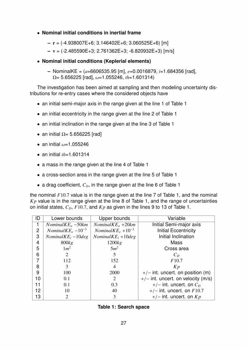
The investigation has been aimed at sampling and then modeling uncertainty dis-

tributions for re-entry cases where the considered objects have

• an initial semi-major axis in the range given at the line 1 of Table 1

• an initial eccentricity in the range given at the line 2 of Table 1

• an initial inclination in the range given at the line 3 of Table 1

• an initial Ω= 5.656225 [rad]

• an initial ω=1.055246

• an initial th=1.601314

• a mass in the range given at the line 4 of Table 1

• a cross-section area in the range given at the line 5 of Table 1

• a drag coefficient, CD, in the range given at the line 6 of Table 1

the nominal F10.7 value is in the range given at the line 7 of Table 1, and the nominal

K p value is in the range given at the line 8 of Table 1, and the range of uncertainties

on initial states, CD, F10.7, and K p as given in the lines 9 to 13 of Table 1.

ID Lower bounds Upper bounds Variable

1 NominalKEa −50km NominalKEa +20km Initial Semi-major axis

2 NominalKEe −10−3 NominalKEe +10−3 Initial Eccentricity

3 NominalKEi −10deg NominalKEi +10deg Initial Inclination

4 800kg 1200kg Mass

5 1m2 5m2 Cross area

6 2 5 CD

7 112 152 F10.7

8 3 4 K p

9 100 2000 +/− int. uncert. on position (m)

10 0.1 2 +/− int. uncert. on velocity (m/s)

11 0.1 0.3 +/− int. uncert. on CD

12 10 40 +/− int. uncert. on F10.7

13 2 3 +/− int. uncert. on K p

Table 1: Search space

27

The search space in Table 1 has been sampled ∼ 9300 times. For each sample, an

uncertainty propagation campaign via A-HDMR approach has been carried out, and

a skew-normal distribution has been fitted to the each corresponding PDF of the re-

entry time, and a database with 9300 13-dimensional inputs and 9300 4-dimensional

outputs has been created. (Note that the output matrix contains the three coefficients

defining the skew-normal, plus a translation term to locate the skew-normal close to

the origin). The obtained database has been treated with many different approaches,

to build a meta-model directly mapping the variables in Table 1 to the parameters of

the skew-normal distribution that best fits the re-entry time PDF.

In particular, the following approaches have been used: Feed Forward Artificial

Neural Networks (FF-ANNs) with Bayesian Regularization (BR), with Levenberg-Marquardt

(LM), with Adam, and with L-BFGS back-propagations techniques (the latter two meth-

ods implemented in Python, while the former three use c©Matlab built-in functions).

Moreover, Radial Basis networks, Generalized Radial Basis networks, and the DACE

library for Kriging have been also tested.

5.3. Results

The investigation is still ongoing, but on the basis of current results, it can be said

that the single layer FF-ANN with BR learning is confirmed as a reliable method having

good generalization capabilities, but the learning process is very slow; tested on some

random check sample points not belonging to the database it gives reasonably good

results both when trained with a local sub set of data (1000 points around the check

point), and when trained with the entire database. An example of the performance of

first approach is given in Figure 36, where the estimated skew-normal is compared

with the one fitted on the PDF obtained with the A-HDMR approach. The same case

treated with the FF-ANN-BR considering the entire database is presented in Figure

37.

Figure 36: Skew-normal distribution predicted by local FF-ANN-BR (cyan dots)

compared to the skew-normal (red dots) fitted on the PDF obtained by the A-

HDMR approach (green dots)

28

Figure 37: Skew-normal distribution predicted by local FF-ANN-BR (cyan dots)

compared to the skew-normal (red dots) fitted on the PDF obtained by the A-

HDMR approach (green dots)

6. Conclusion

The paper presents some of the main results and activities to characterize and

propagate the uncertainties on the atmospheric re-entry time of GOCE carried out

within the framework of an ESA ITT project on benchmarking GOCE’s re-entry predic-

tion uncertainties.

Results obtained for the Uncertainty Propagation analyses have pointed out shapes

of the PDFs for the re-entry time depending on the degrees of freedom (3 or 6). In

particular, when attitude is considered, the function linking the re-entry time to the

considered uncertainties of the uncontrolled GOCE can be multi-modal, resulting into

a non-standard PDF with multiple peaks. Distributions become unimodal if a single

regime (stable or pure tumbling) lasts during most of the re-entry, and in this case dis-

tributions obtained via 3DoF propagation can match relatively well the ones obtained

with the 6DoF propagation.

Two different uncertainty quantification/characterization approaches have been also

proposed. The same interpolation techniques used for computationally cheap, non-

intrusive methods for UP, allowed the development of two methods based on direct

optimization approaches, namely the Boundary Set Approach and the Inverse Uncer-

tainty Quantification. Both have been tested, but not fully exploited. Most of the test

analyses were carried out by using approximated UP techniques, but there is still no

information on the output distribution to match.

Moreover, a new approach to empirical acceleration has been tested on arcs of

GOCEs trajectory. Instead of a time series, the function is written as a multivariate

polynomial, whose variables are the components of the state vector. There is a gain

in generality as the polynomial coefficients derived from measurements are less time-

dependent. Here, the modified Hill variables were used to represent the state, as most

of them vary slowly with time. Calculating the coefficients of the empirical acceleration

is done via an optimization process, where the trajectory is constrained to pass through

way-points given by the measurements. Thus, the results are highly dependent on the29

parameters of the problem (number of coefficients, tightness of the box constraints,

etc.). Uncertainty in the initial conditions is handled by computing as many sets of

coefficients as there are samples. Analyzing the resulting probability distributions then

helps to understand where the missing components of the dynamical model lye.

Finally, some preliminary results on the use use of meta-modeling techniques to

directly map a range of initial states and model uncertainties into re-entry time windows

distributions, providing with a very fast characterization of the output PDF not requiring

any propagation at all. Preliminary results shown in this paper tend to confirm that this

is possible, but the approach should be better implemented and further tested in the

future.

Follow-up work includes: 1) the use of a more complex model for the uncertainty

acting on the atmospheric parameters: more precisely, instead of having them con-

stant during each propagation, one could allow variations over time following some

probabilistic law; 2) the finalization of the meta-modeling approach to learn the coeffi-

cients of the skew-normal distributions; and 3) the exploration of the use of the same

meta-modeling techniques to learn the re-entry dynamics and map the initial condi-

tions and the object and atmosphere properties to the re-entry time.

Acknowledgments

This work was carried out under ESA Contract No. 4000115172/15/F/MOS Bench-

marking re-entry prediction uncertainties. The support of the ESA Space Debris Office

is gratefully acknowledged. The authors are particularly thankful to Stefano Cicalo,

James Beck and Ian Holbrough for their precious comments and suggestions during

the project.

The authors also acknowledge the use of the 3DoF and 6DoF propagators of Bel-

stead Research Ltd for the analyses presented in Section 2 , and the EPSRC funded

ARCHIE-WeSt High Performance Computer (www.archie-west.ac.uk). EPSRC grant

no. EP/K000586/1.

References

[1] R. Armellin, P. Di Lizia, F. Bernelli-Zazzera, and M. Berz. Asteroid close encounters characteriza-

tion using differential algebra: the case of apophis. Celestial Mechanics and Dynamical Astronomy,

107(4):451–470, 2010.

[2] J. Beck, I. Holbrough, M. Vasile, E. Minisci, and R. Serra. Debris evolution uncertainty quantifica-

tion. UKSA NSTP Pathfinder Final Report, December 2016.

[3] I. G. Izsak. A note on perturbation theory. The Astronomical Journal, 68:559–561, 1963.

[4] M. Kubicek, E. Minisci, and M. Cisternino. High dimensional sensitivity analysis using surrogate

modeling and high dimensional model representation. International Journal for Uncertainty Quan-

tification, 5(5):393–414, 2015.

[5] P. M. Mehta, M. Kubicek, E. Minisci, and M. Vasile. Sensitivity analysis and probabilistic re-entry

modeling for debris using high dimensional model representation based uncertainty treatment.

Advances in Space Research, 59(1):193–211, 2017.

[6] E. Minisci and M. Vasile. Adaptive inflationary differential evolution algorithm. In Congress on

Evolutionary Computation (CEC2014), 2014.

[7] O. Montenbruck and E. Gill. Satellite orbits. Springer, 2, 2000.

[8] C. Ortega Absil, R. Serra, A. Riccardi, and M. Vasile. De-orbiting and re-entry analysis with gen-

eralised intrusive polynomial expansions. In 67th International Astronautical Congress, 2016.

[9] C. Tardioli, M. Kubicek, M. Vasile, E. Minisci, and A. Riccardi. Comparison of non-intrusive ap-

proaches to uncertainty propagation in orbital mechanics. In Proceedings of AAS/AIAA Astrody-

namics Specialist Conference, Vail, Colorado, 2015.

30

[10] M. Vasile, E. Minisci, R. Serra, J. Beck, and I. Holbrough. Analysis of the de-orbiting and re-entry of

space objects with high area to mass ratio. In Proceedings of AAS/AIAA Astrodynamics Specialist

Conference, Long Beach, California, 2016.

[11] M. Vasile, C. Tardioli, A. Riccardi, and H. Yamakawa. Collision avoidance as a robust reachability

problem under model uncertainty. In Proceedings of 26th AAS/AIAA Space Flight Mechanics

Meeting, 2016.

[12] M. Vetrisano and M. Vasile. Analysis of spacecraft disposal solutions from lpo to the moon with

high order polynomial expansions. Advances in Space Research, 60(1):38–56, 2017.

31

View publication statsView publication stats