Mining Social Network Graphs Debapriyo Majumdar Data Mining – Fall 2014 Indian Statistical...

Mining Social Network Graphs

Debapriyo Majumdar

Data Mining – Fall 2014

Indian Statistical Institute Kolkata

November 13, 17, 2014

2

Social Network

No introduction required

Really?

We still need to understand a few properties

disclaimer: the brand logos are used here entirely for educational purpose

3

Social Network A collection of entities

– Typically people, but could be something else too

At least one relationship between entities of the network– For example: friends– Sometimes boolean: two people are either friends or they are not– May have a degree– Discrete degree: friends, family, acquaintances, or none– Degree – real number: the fraction of the average day that two people

spend talking to each other

An assumption of nonrandomness or locality– Hard to formalize– Intuition: that relationships tend to cluster– If entity A is related to both B and C, then the probability that B and C

are related is higher than average (random)

4

Social Network as a Graph

Check for the non-randomness criterion In a random graph (V,E) of 7 nodes and 9 edges, if XY is an edge, YZ

is an edge, what is the probability that XZ is an edge?– For a large random graph, it would be close to |E|/(|V|C2) = 9/21 ~ 0.43

– Small graph: XY and YZ are already edges, so compute within the rest

– So the probability is (|E|−2)/(|V|C2−2) = 7/19 = 0.37

Now let’s compute what is the probability for this graph in particular

A B

C

D E

G FA graph with boolean (friends) relationship

Example courtesy: Leskovec, Rajaraman and Ullman

5

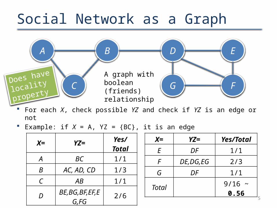
Social Network as a Graph

For each X, check possible YZ and check if YZ is an edge or not Example: if X = A, YZ = {BC}, it is an edge

A B

C

D E

G FA graph with boolean (friends) relationship

X= YZ= Yes/Total

A BC 1/1

B AC, AD, CD 1/3

C AB 1/1

DBE,BG,BF,EF,

EG,FG 2/6

X= YZ= Yes/Total

E DF 1/1

F DE,DG,EG 2/3

G DF 1/1

Total 9/16 ~ 0.56

Does have

locality

property

6

Types of Social (or Professional) Networks

Of course, the “social network”. But also several other types Telephone network Nodes are phone numbers AB is an edge if A and B talked over phone within the last one week, or

month, or ever Edges could be weighted by the number of times phone calls were made,

or total time of conversation

A B

C

D E

G F

7

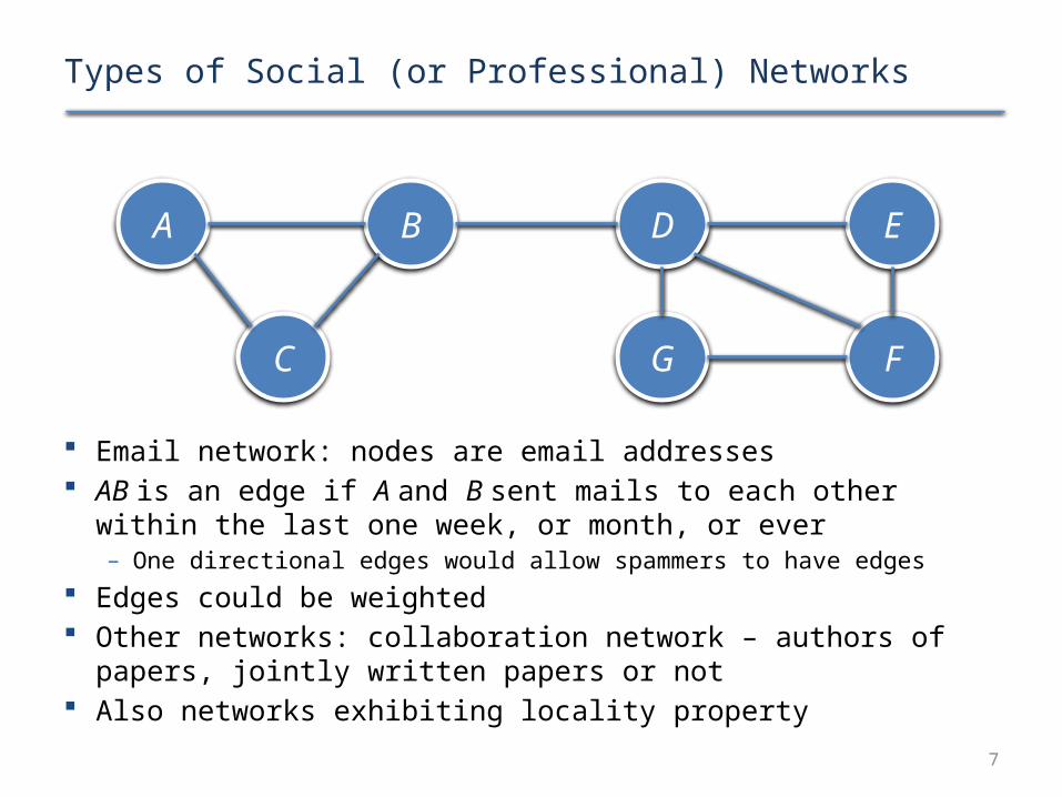
Types of Social (or Professional) Networks

Email network: nodes are email addresses AB is an edge if A and B sent mails to each other within the last one week,

or month, or ever– One directional edges would allow spammers to have edges

Edges could be weighted Other networks: collaboration network – authors of papers, jointly written

papers or not Also networks exhibiting locality property

A B

C

D E

G F

8

Clustering of Social Network Graphs Locality property there are clusters Clusters are communities

– People of the same institute, or company– People in a photography club– Set of people with “Something in common” between them

Need to define a distance between points (nodes) In graphs with weighted edges, different distances exist For graphs with “friends” or “not friends” relationship

– Distance is 0 (friends) or 1 (not friends)– Or 1 (friends) and infinity (not friends)– Both of these violate the triangle inequality– Fix triangle inequality: distance = 1 (friends) and 1.5 or 2 (not

friends) or length of shortest path

9

Traditional Clustering

Intuitively, two communities Traditional clustering depends on the distance

– Likely to put two nodes with small distance in the same cluster – Social network graphs would have cross-community edges– Severe merging of communities likely

May join B and D (and hence the two communities) with not so low probability

A B

C

D E

G F

10

Betweenness of an Edge

Betweenness of an edge AB: #of pairs of nodes (X,Y) such that AB lies on the shortest path between X and Y– There can be more than one shortest paths between X and Y– Credit AB the fraction of those paths which include the edge AB

High score of betweenness means?– The edge runs “between” two communities

Betweenness gives a better measure– Edges such as BD get a higher score than edges such as AB

Not a distance measure, may not satisfy triangle inequality. Doesn’t matter!

A B

C

D E

G F

11

The Girvan – Newman Algorithm Step 1 – BFS: Start at a node X,

perform a BFS with X as root

Observe: level of node Y = length of shortest path from X to Y

Edges between level are called “DAG” edges– Each DAG edge is part of at

least one shortest path from X

Step 2 – Labeling: Label each node Y by the number of shortest paths from X to Y

Calculate betweenness of edges

A

B

C

D

E

G

FLevel 1

Level 2

Level 3

1

1

1

12

1 1

12

The Girvan – Newman AlgorithmStep 3 – credit sharing: Each leaf node gets credit 1 Each non-leaf node gets 1 +

sum(credits of the DAG edges to the level below)

Credit of DAG edges: Let Yi (i=1, … , k) be parents of Z, pi = label(Yi)

Calculate betweenness of edges

A

B

C

D

E

G

FLevel 1

Level 2

Level 3

1

1

1

12

1 11 1

13

1 1

Intuition: a DAG edge YiZ gets the share of credit of Z proportional to the #of shortest paths from X to Z going through YiZ

Finally: Repeat Steps 1, 2 and 3 with each node as root. For each edge, betweenness = sum credits obtained in all iterations / 2

3 0.5 0.5

4.51.5

4.5 1.5

13

Computation in practice Complexity: n nodes, e edges

– BFS starting at each node: O(e) – Do it for n nodes– Total: O(ne) time– Very expensive

Method in practice– Choose a random subset W of the nodes – Compute credit of each edge starting at each node in W– Sum and compute betweenness– A reasonable approximation

14

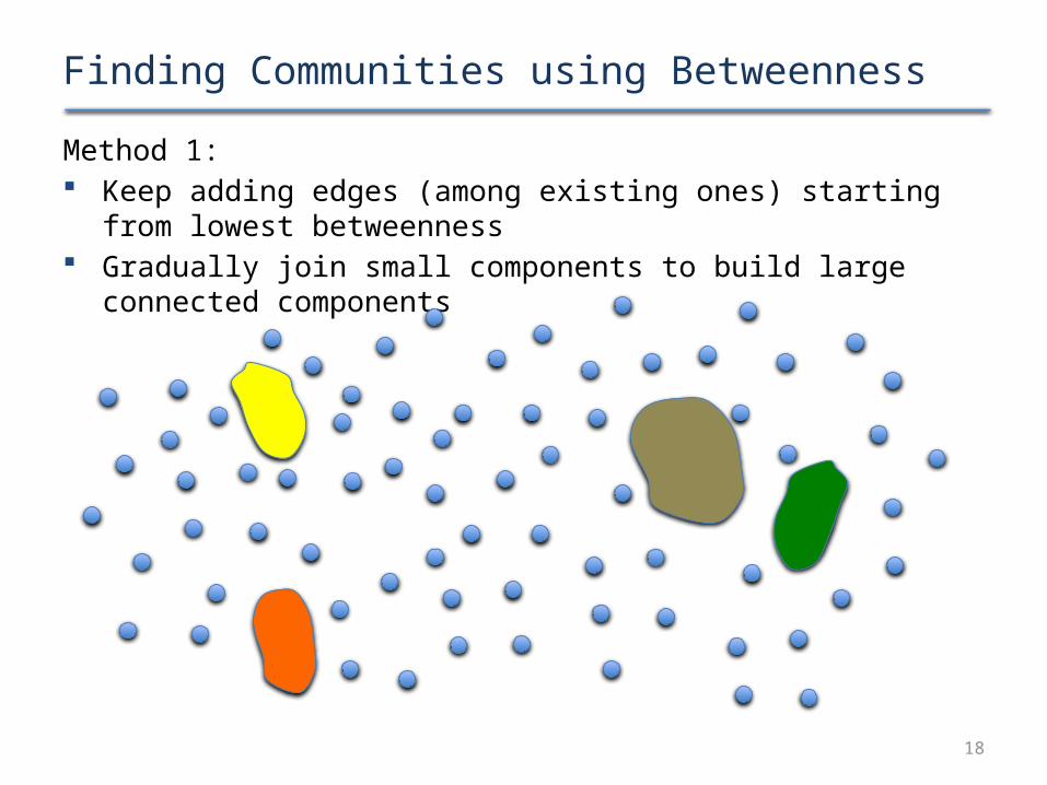
Finding Communities using BetweennessMethod 1: Keep adding edges (among existing ones) starting from lowest betweenness Gradually join small components to build large connected components

15


16


17


18


19


20

Finding Communities using BetweennessMethod 2: Start from all existing edges. The graph may look like one big component. Keep removing edges starting from highest betweenness Gradually split large components to arrive at communities

21


22


At some point, removing the edge with highest betweenness would split the graph into separate components

23

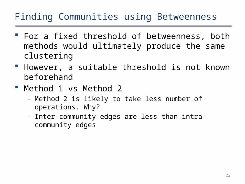
Finding Communities using Betweenness For a fixed threshold of betweenness, both methods would

ultimately produce the same clustering However, a suitable threshold is not known beforehand Method 1 vs Method 2

– Method 2 is likely to take less number of operations. Why?– Inter-community edges are less than intra-community edges

24

Triangles in Social Network Graph Number of triangles in a social network graph is expected to

be much larger than a random graph with the same size– The locality property

Counting the number of triangles– How much the graph looks like a social network– Age of community

• A new community forms• Members bring in their like minded friends• Such new members are expected to eventually connect to

other members directly

25

Triangle Counting Algorithm

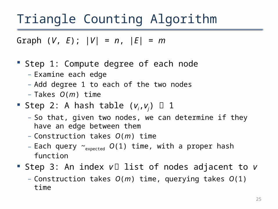
Graph (V, E); |V| = n, |E| = m

Step 1: Compute degree of each node– Examine each edge– Add degree 1 to each of the two nodes– Takes O(m) time

Step 2: A hash table (vi,vj) 1– So that, given two nodes, we can determine if they have an edge

between them– Construction takes O(m) time

– Each query ~expected O(1) time, with a proper hash function

Step 3: An index v list of nodes adjacent to v– Construction takes O(m) time, querying takes O(1) time

26

Counting Heavy Hitter Triangles Heavy hitter node: a node with degree ≥ √m Note: there are at most 2√m heavy hitter nodes– More than 2√m nodes total degree > 2m (but |E| = m)

Heavy hitter triangle: triangle with all 3 heavy hitter nodes Number of possible heavy hitter triangles: at most 2√mC3 ~

O(m3/2) For each possible triangle, use hash table (step 2) to check if

all three edges exist Takes O(m3/2) time

27

Counting other Triangles Consider an ordering of nodes vi << vj if

– Either degree(vi) < degree(vj), and

– If degree(vi) = degree(vj) then i < j

For each edge (vi,vj)– If both nodes are heavy hitters, skip (already done)

– Suppose vi is not a heavy hitter

– Find nodes w1,w2,…,wk which are adjacent to vi (using node adjacent nodes index, step 3) [Takes O(k) time]

– For each wl , l = 1, … , k check if edge vjwl exist, in O(1) time, total O(k) time

– Count the triangle {vi vj wl} if and only if

• Edge vjwl exists

• Also vi << wl

– Total time for each edge (vi,vj) is O(√m)

– There are m edges, total time is O(m3/2) time

28

OptimalityWorst case scenario If G is a complete graph Number of triangles = mC3 ~ O(m3/2)

Cannot even enumerate all triangles in less than O(m3/2) Hence it is the lower bound for computing all triangles

If G is sparse Consider a complete graph G’ with n nodes, m edges Note that m = nC2 = O(n2)

Construct G from G’ by adding a chain of length n2

The number of triangles remain the same, O(m3/2) The number of edges remain of the same order O(m) G is quite sparse, lowering edge to node ratio Still cannot compute the triangles in less than O(m3/2) time

29

Directed Graphs in (Social) Networks Set of nodes V and directed edges (arcs) u v The web: pages link to other pages Persons made calls to other persons Twitter, Google+: people follow other people All undirected graphs can be considered as directed– Think of each edge as bidirectional

30

Paths and Neighborhoods Path of length k: a sequence of nodes v0,v1,…,vk from v0 to vk so

that vi vi+1 is an arc for i = 0, …, k – 1

Neighborhood N(v,d) of radius d for a node v: set of all nodes w such that there is a path from v to w of length ≤ d

For a set of nodes V, N(V,d):= {w | there is a path of length ≤ d from some v in V to w}

Neighborhood profile of a node v: sequence of sizes of its neighborhoods of radius d = 1, 2, …; that is

|N(v,1)|, |N(v,2)|, |N(v,3)|, …

31

Neighborhood Profile

Neighborhood profile of B

N(“B”,1) = 4

N(“B”,2) = 7

A B

C

D E

G F

Neighborhood profile of A

N(“A”,1) = 3

N(“A”,2) = 4

N(“A”,3) = 7

32

Diameter of a Graph Diameter of a graph G(V,E): the smallest integer d

such that for any two nodes v, w in V, there is a path of length at most d from v to w– Only makes sense for strongly connected graphs– Can reach any node from any node

The web graph: not strongly connected– But there is a large strongly connected component

The six degrees of separation conjecture– The diameter of the graph of the people in the world is six

33

Diameter and Neighborhood Profile Neighborhood profile of a node v

|N(v,1)|, |N(v,2)|, |N(v,3)|, … … Denote this k as d(v) If G is a complete graph, d(v) = 1 Diameter of G is maxv{d(v)}

|V| = N(v,k) for some k

34

Reference Mining of Massive Datasets, by Leskovec, Rajaraman

and Ullman, Chapter 10

Mining Social Network Graphs Debapriyo Majumdar Data Mining – Fall 2014 Indian Statistical...

Documents

Transcript of Mining Social Network Graphs Debapriyo Majumdar Data Mining – Fall 2014 Indian Statistical...