Minimum Volume Confidence Regions for a

Multivariate Normal Mean Vector

Bradley Efron

Abstract

Since Stein’s original proposal in 1962, a series of papers have constructed con-

fidence regions of smaller volume than the standard spheres for the mean vector of

a multivariate normal distribution. A general approach to this problem is developed

here, and used to calculate a lower bound on the attainable volume. Bayes and fiducial

methods are involved in the calculation. Scheffe-type problems are used to show that

low volume by itself does not guarantee favorable inferential properties.

Key Words James-Stein estimator, Fisher-von Mises distribution, non-central chi, Scheffe

intervals

1. Introduction Stein (1962) conjectured and heuristically demonstrated confidence

regions for a multivariate normal mean vector having everywhere smaller volume than the

standard ones. A variety of ingenious constructions has verified Stein’s conjecture, including

those of Faith (1976), Berger (1980), Casella and Hwang (1983), Tseng and Brown (1997),

and Samworth (2005). This paper concerns a general approach to multivariate normal mean

confidence regions, a bound on the minimally attainable volume, and some related inferential

questions.

Let x be an n-dimensional normal vector with mean µ and covariance matrix the iden-

tity,

x ∼ N(µ, I), (1.1)

and define r and ρ as the ordinary Euclidean length of x and µ,

r = ‖x‖ and ρ = ‖µ‖. (1.2)

The standard level α confidence region for µ given x is the sphere

C0x = {µ : ‖µ − x‖ ≤ χ(α)

n }, (1.3)

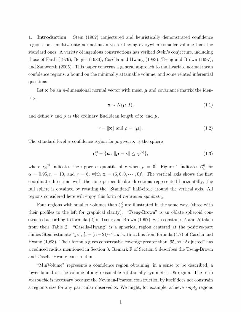
where χ(α)n indicates the upper α quantile of r when ρ = 0. Figure 1 indicates C0

x for

α = 0.95, n = 10, and r = 6, with x = (6, 0, 0, · · · , 0)′. The vertical axis shows the first

coordinate direction, with the nine perpendicular directions represented horizontally; the

full sphere is obtained by rotating the “Standard” half-circle around the vertical axis. All

regions considered here will enjoy this form of rotational symmetry.

Four regions with smaller volumes than C0x are illustrated in the same way, (three with

their profiles to the left for graphical clarity). “Tseng-Brown” is an oblate spheroid con-

structed according to formula (2) of Tseng and Brown (1997), with constants A and B taken

from their Table 2. “Casella-Hwang” is a spherical region centered at the positive-part

James-Stein estimate “js”, [1− (n− 2)/r2]+x, with radius from formula (4.7) of Casella and

Hwang (1983). Their formula gives conservative coverage greater than .95, so “Adjusted” has

a reduced radius mentioned in Section 3. Remark F of Section 5 describes the Tseng-Brown

and Casella-Hwang constructions.

“MinVolume” represents a confidence region obtaining, in a sense to be described, a

lower bound on the volume of any reasonable rotationally symmetric .95 region. The term

reasonable is necessary because the Neyman-Pearson construction by itself does not constrain

a region’s size for any particular observed x. We might, for example, achieve empty regions

1

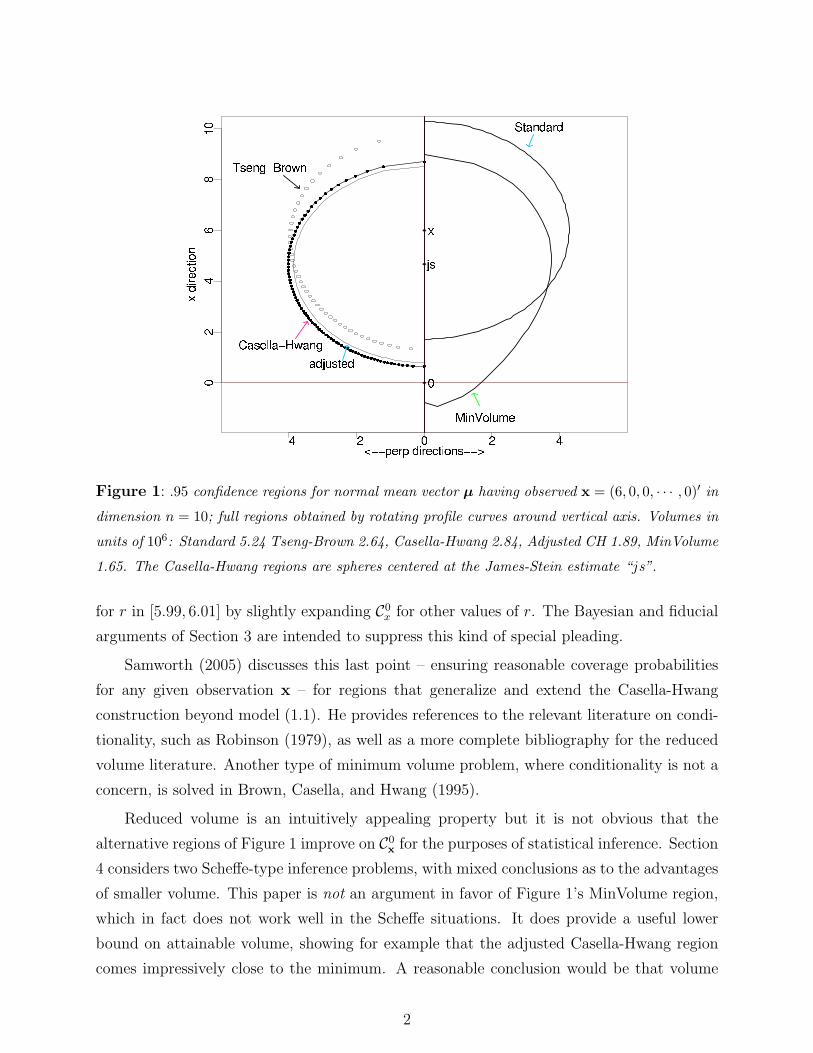
Figure 1: .95 confidence regions for normal mean vector µ having observed x = (6, 0, 0, · · · , 0)′ in

dimension n = 10; full regions obtained by rotating profile curves around vertical axis. Volumes in

units of 106: Standard 5.24 Tseng-Brown 2.64, Casella-Hwang 2.84, Adjusted CH 1.89, MinVolume

1.65. The Casella-Hwang regions are spheres centered at the James-Stein estimate “js”.

for r in [5.99, 6.01] by slightly expanding C0x for other values of r. The Bayesian and fiducial

arguments of Section 3 are intended to suppress this kind of special pleading.

Samworth (2005) discusses this last point – ensuring reasonable coverage probabilities

for any given observation x – for regions that generalize and extend the Casella-Hwang

construction beyond model (1.1). He provides references to the relevant literature on condi-

tionality, such as Robinson (1979), as well as a more complete bibliography for the reduced

volume literature. Another type of minimum volume problem, where conditionality is not a

concern, is solved in Brown, Casella, and Hwang (1995).

Reduced volume is an intuitively appealing property but it is not obvious that the

alternative regions of Figure 1 improve on C0x for the purposes of statistical inference. Section

4 considers two Scheffe-type inference problems, with mixed conclusions as to the advantages

of smaller volume. This paper is not an argument in favor of Figure 1’s MinVolume region,

which in fact does not work well in the Scheffe situations. It does provide a useful lower

bound on attainable volume, showing for example that the adjusted Casella-Hwang region

comes impressively close to the minimum. A reasonable conclusion would be that volume

2

reduction has gone about as far as it can, and that increased attention should be paid to

specific inferential properties.

The paper concludes in Section 5 with derivations of the previous results as well as some

further remarks.

2. A General Construction This paper follows the literature in only considering con-

fidence regions having rotational symmetry around the axis determined by x , as indicated

in Figure 1. Rotational symmetry allows us to reduce vectorial situation (1.1) to the scalar

problem of finding confidence intervals for ρ based on r, (1.2), as shown next. The rationale

for Tseng-Brown and Casella-Hwang constructions becomes more transparent in the (ρ, r)

framework.

The distribution of r = ‖x‖ given ρ = ‖µ‖ is “non-central chi”, say r ∼ χn(ρ), the

square root of a non-central chi-squared distribution χ2n(ρ2). We denote the density of r

given ρ by

fρ(r), r ≥ 0 (2.1)

with Fρ(r) as the corresponding cumulative distribution function (cdf).

Suppose aρ(r) is a function satisfying

0 ≤ aρ(r) ≤ 1 (2.2)

for all non-negative ρ and r, with∫ ∞

0

aρ(r)fρ(r)dr = α for all ρ ≥ 0. (2.3)

Then aρ(r) defines level α randomized confidence intervals I(r) for ρ given r : value ρ

exists in I(r) with probability aρ(r). Non-randomized intervals have aρ(r) equal 0 or 1. For

instance the usual two-sided 0.95 intervals are defined in terms of the quantiles of χn(ρ) by

aρ(r) =

1 r ∈ [χn(ρ)(.025), χn(ρ)(.975)]

if

0 otherwise

(2.4)

We will call aρ(r) satisfying (2.2)-(2.3) an “inclusion function”.

Every inclusion function defines a non-randomized set of level α confidence regions for

µ given x ∼ N(µ, I). The construction, which figures implicitly in Casella and Hwang

3

(1983), begins with the Fisher-von Mises distribution for the angle “γ” between x and µ

(conditional on both µ and r). In terms of z = cos(γ), the Fisher-von Mises density is

crρerρz(1 − z2)

n−32 for − 1 ≤ z ≤ 1, (2.5)

see Remark A of Section 5. The constant

crρ =

[ ∫ 1

−1

erρz(1 − z2)n−3

2 dz

]−1

(2.6)

can be expressed in terms of modified Bessel functions, as in Downs (1966).

For γ an angle in [0, π] define Sµ(γ, r) as the spherical cap of angular radius γ centered

at r · (µ/ρ), (the multiple of µ having length r),

Sµ(γ, r) = {x : ‖x‖ = r andx′µ

rρ≥ cos(γ)}. (2.7)

(Notice that x′µ/rρ is the cosine of the angle between x and µ.) The conditional probability

content of Sµ(γ, r) given µ and r is

Probµ{x ∈ Sµ(γ, r)|r} =

∫ 1

cos(γ)

crρerρz(1 − z2)

n−32 dz (2.8)

according to (2.5), increasing from 0 to 1 as γ increases from 0 to π. For any value of the

inclusion function aρ(r) there is a unique angle γρ(r), with cosine zρ(r), such that

aρ(r) =

∫ 1

zρ(r)

crρerρz(1 − z2)

n−32 dz, (2.9)

i.e. such that Sµ(γρ(r), r) has conditional probability content aρ(r).

We can now define a level α acceptance region Aµ (for testing the hypothesis that x’s

mean vector equals µ) as a union of spherical caps,

Aµ = ∪r≥0

Sµ(γρ(r), r), (2.10)

so that

Probµ{x ∈ Aµ} = α; (2.11)

(2.11) follows immediately from (2.3) since the rth spherical cap has conditional probability

aρ(r) of containing x .

4

The level α acceptance regions Aµ can be inverted to give confidence regions Cx accord-

ing to the usual Neyman construction:

Cx = ∪ρ≥0

Sx(γρ(r), ρ). (2.12)

Here Sx(γρ(r), ρ) is a spherical cap of angular radius γρ(r) centered at ρ · (x/r), the multiple

of x having length ρ; the level α confidence region Cx is the union of such caps over all

choices of ρ. The fact that the same function γρ(r) figures in both (2.10) and (2.12) reflects

the circular geometry of the spherical caps.

To summarize, any inclusion function aρ(r), (2.1)-(2.3), generates a set of non-randomized

level α acceptance regions Aµ and corresponding confidence regions Cx. We can “reverse

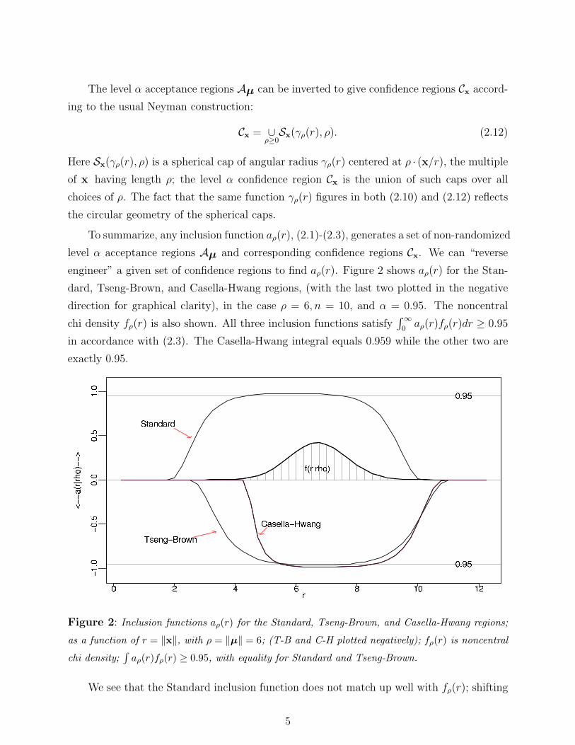
engineer” a given set of confidence regions to find aρ(r). Figure 2 shows aρ(r) for the Stan-

dard, Tseng-Brown, and Casella-Hwang regions, (with the last two plotted in the negative

direction for graphical clarity), in the case ρ = 6, n = 10, and α = 0.95. The noncentral

chi density fρ(r) is also shown. All three inclusion functions satisfy∫ ∞

0aρ(r)fρ(r)dr ≥ 0.95

in accordance with (2.3). The Casella-Hwang integral equals 0.959 while the other two are

exactly 0.95.

Figure 2: Inclusion functions aρ(r) for the Standard, Tseng-Brown, and Casella-Hwang regions;

as a function of r = ‖x‖, with ρ = ‖µ‖ = 6; (T-B and C-H plotted negatively); fρ(r) is noncentral

chi density;∫

aρ(r)fρ(r) ≥ 0.95, with equality for Standard and Tseng-Brown.

We see that the Standard inclusion function does not match up well with fρ(r); shifting

5

it rightwards along the r axis gives a better match, allowing us to reduce aρ(r) while still

satisfying (2.3). This is what the Tseng-Brown and Casella-Hwang constructions both do.

Doing so for all ρ gives smaller confidence regions Cx, in a way made clearer in Section 3.

At this point we might try selecting aρ(r) so as to minimize the volume of the acceptance

region Aµ subject to∫

aρ(r)fρ(r)dr = α. It turns out that this yields Aµ = {x : ‖x −µ‖ ≤ χ

(α)n }, in other words the standard spherical acceptance region connected with (1.3);

see Remark C, Section 5. This, perhaps, sharpens the surprise that Stein’s conjecture is

true. The nonstandard constructions of Figure 1 increase acceptance regions but decrease

confidence regions, as shown in Section 3.

Algorithm (2.2)-(2.12) provides a very flexible recipe for constructing confidence regions

for a multivariate normal mean vector, too flexible from the point of view of actual appli-

cation. Section 3 considers, along with Bayesian and fiducial regions, a restricted class of

inclusion functions, “percentile rules”,

aρ(r) = A(Fρ(r)), (2.13)

where Fρ(r) is the noncentral chi cdf, while A(·) is a function satisfying 0 ≤ A(F ) ≤ 1 and∫ 1

0

A(F )dF = α (2.14)

The non-randomized interval (2.4) is a percentile rule.

Percentile rules are a function of only one variable, rather than two for general rules

aρ(r). We see that aρ(r) = A(Fρ(r)) satisfies (2.2)-(2.3), the latter from∫ ∞

0

A(Fρ(r))fρ(r)dr =

∫ ∞

0

A(Fρ(r))∂Fρ(r)

∂rdr

=

∫ 1

0

A(F )dF = α.

(2.15)

3. Bayes and Fiducial Regions Figure 2 reduces the construction of acceptance regions

for x ∼ N(µ, I) to that of forming acceptance intervals for r ∼ χn(ρ). This section concerns

the corresponding theory for confidence regions, from which the MinVolume region of Figure

1 will be derived. Doing so requires Bayesian and fiducial ideas, since frequentist methods

by themselves do not constrain the size of a level α region Cx for any particular x . We

continue to denote r = ‖x‖ and ρ = ‖µ‖.The confidence density for ρ given r, Efron (1993), is defined in terms of the cdf Fρ(r)

of a χn(ρ) distribution,

g†(ρ|r) = − ∂

∂ρFρ(r), (3.1)

6

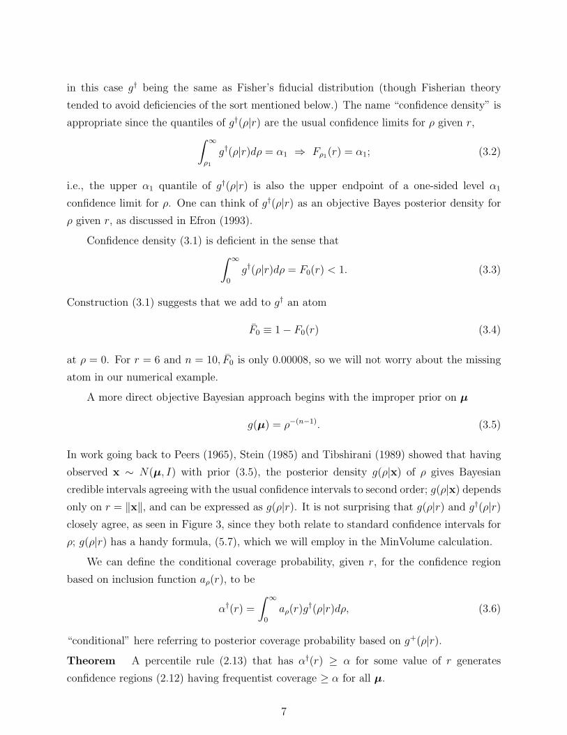
in this case g† being the same as Fisher’s fiducial distribution (though Fisherian theory

tended to avoid deficiencies of the sort mentioned below.) The name “confidence density” is

appropriate since the quantiles of g†(ρ|r) are the usual confidence limits for ρ given r,∫ ∞

ρ1

g†(ρ|r)dρ = α1 ⇒ Fρ1(r) = α1; (3.2)

i.e., the upper α1 quantile of g†(ρ|r) is also the upper endpoint of a one-sided level α1

confidence limit for ρ. One can think of g†(ρ|r) as an objective Bayes posterior density for

ρ given r, as discussed in Efron (1993).

Confidence density (3.1) is deficient in the sense that∫ ∞

0

g†(ρ|r)dρ = F0(r) < 1. (3.3)

Construction (3.1) suggests that we add to g† an atom

F0 ≡ 1 − F0(r) (3.4)

at ρ = 0. For r = 6 and n = 10, F0 is only 0.00008, so we will not worry about the missing

atom in our numerical example.

A more direct objective Bayesian approach begins with the improper prior on µ

g(µ) = ρ−(n−1). (3.5)

In work going back to Peers (1965), Stein (1985) and Tibshirani (1989) showed that having

observed x ∼ N(µ, I) with prior (3.5), the posterior density g(ρ|x) of ρ gives Bayesian

credible intervals agreeing with the usual confidence intervals to second order; g(ρ|x) depends

only on r = ‖x‖, and can be expressed as g(ρ|r). It is not surprising that g(ρ|r) and g†(ρ|r)closely agree, as seen in Figure 3, since they both relate to standard confidence intervals for

ρ; g(ρ|r) has a handy formula, (5.7), which we will employ in the MinVolume calculation.

We can define the conditional coverage probability, given r, for the confidence region

based on inclusion function aρ(r), to be

α†(r) =

∫ ∞

0

aρ(r)g†(ρ|r)dρ, (3.6)

“conditional” here referring to posterior coverage probability based on g+(ρ|r).Theorem A percentile rule (2.13) that has α†(r) ≥ α for some value of r generates

confidence regions (2.12) having frequentist coverage ≥ α for all µ.

7

Figure 3: Confidence density g†(ρ|r) (3.1) for r = 6, n = 10 (solid curve); dots show Bayes

posterior density g(ρ|r) from prior (3.5).

Proof For a percentile rule aρ(r) = A(Fρ(r)),

α ≤ α†(r) = −∫ ∞

0

A(Fρ(r))∂Fρ(r)

∂ρdρ =

∫ F0(r)

0

A(F )dF

≤∫ 1

0

A(F )dF =

∫ ∞

0

aρ(r)fρ(r)dr

(3.7)

for all ρ, as in (2.15); this last quantity is the acceptance probability (2.11). In what follows

we will use the Theorem to construct frequentist confidence regions from a rule aρ(r0) that

minimizes volume at a given value r = r0.

Prior (3.5) gives a formal Bayes version of the conditional coverage probability (3.6),

α(r) =

∫ ∞

0

aρ(r)g(ρ|r)dρ; (3.8)

α(r) nearly equals α†(r) for situations like that of Figure 3.

We wish to compare various confidence regions for a given value of x , or equivalently

(for rotationally symmetric regions) for a given value of r = ‖x‖. The idea of what follows

is to enforce fair comparison by insisting on equal conditional coverage, say α†(r) = 0.95.

Samworth (2005) stresses the importance of good conditional coverage properties.

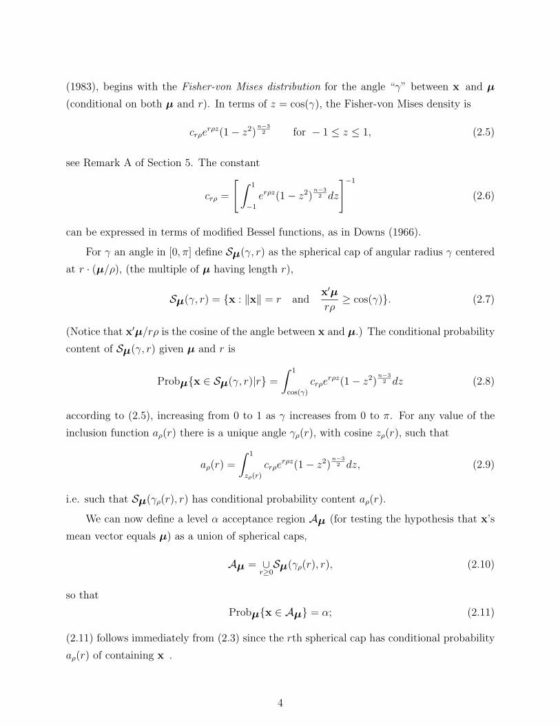
Figure 4 plots inclusion functions aρ(r) for the Standard, Tseng-Brown, Casella-Hwang,

and MinVolume regions of Figure 1, now with ρ varying and r = 6 fixed (n = 10 and

8

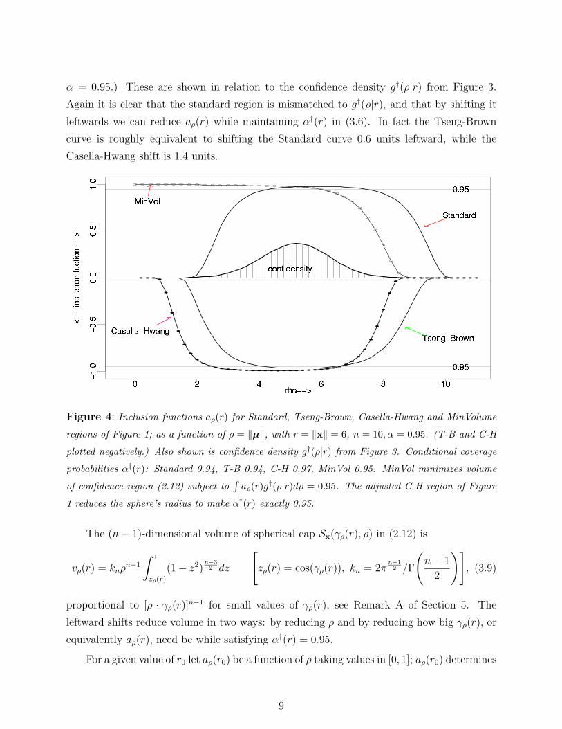
α = 0.95.) These are shown in relation to the confidence density g†(ρ|r) from Figure 3.

Again it is clear that the standard region is mismatched to g†(ρ|r), and that by shifting it

leftwards we can reduce aρ(r) while maintaining α†(r) in (3.6). In fact the Tseng-Brown

curve is roughly equivalent to shifting the Standard curve 0.6 units leftward, while the

Casella-Hwang shift is 1.4 units.

Figure 4: Inclusion functions aρ(r) for Standard, Tseng-Brown, Casella-Hwang and MinVolume

regions of Figure 1; as a function of ρ = ‖µ‖, with r = ‖x‖ = 6, n = 10, α = 0.95. (T-B and C-H

plotted negatively.) Also shown is confidence density g†(ρ|r) from Figure 3. Conditional coverage

probabilities α†(r): Standard 0.94, T-B 0.94, C-H 0.97, MinVol 0.95. MinVol minimizes volume

of confidence region (2.12) subject to∫

aρ(r)g†(ρ|r)dρ = 0.95. The adjusted C-H region of Figure

1 reduces the sphere’s radius to make α†(r) exactly 0.95.

The (n − 1)-dimensional volume of spherical cap Sx(γρ(r), ρ) in (2.12) is

vρ(r) = knρn−1

∫ 1

zρ(r)

(1− z2)n−3

2 dz

[zρ(r) = cos(γρ(r)), kn = 2π

n−12 /Γ

(n − 1

2

)], (3.9)

proportional to [ρ · γρ(r)]n−1 for small values of γρ(r), see Remark A of Section 5. The

leftward shifts reduce volume in two ways: by reducing ρ and by reducing how big γρ(r), or

equivalently aρ(r), need be while satisfying α†(r) = 0.95.

For a given value of r0 let aρ(r0) be a function of ρ taking values in [0, 1]; aρ(r0) determines

9

zρ(r0) as in (2.9) and then a confidence region (2.12) having volume

V (r0) =

∫ ∞

0

vρ(r0)dρ. (3.10)

The “MinVol” curve in Figure 4 is the function aρ(r0) that minimizes V (r0) subject to the

conditional coverage constraint

α†(r0) =

∫ ∞

0

aρ(r0)g†(ρ|r0)dρ = 0.95 (r0 = 6). (3.11)

The corresponding confidence region Cx is labeled “MinVolume” in Figure 1.

In order to extend aρ(r0) to other values of r, define the function A by

A(Fρ(r0)) = aρ(r0). (3.12)

Then according to our previous results, (2.15) and the Theorem, aρ(r) = A(Fρ(r)) is an

inclusion function whose corresponding confidence regions have coverage ≥ 0.95. We have

now constructed a rotationally symmetric system of 0.95 confidence regions having minimum

volume at r0 = 6 among those with α†(r0) = 0.95.

The actual calculation of the MinVolume inclusion function aρ(r0) appears in Remark

B of Section 5; aρ(r) looks peculiar in Figure 4, approaching 1 instead of 0 as ρ goes to 0

(causing the MinVolume region to contain the origin in Figure 1). This is possible because

the spherical shell volume v(ρ), (3.9), goes to zero very rapidly near ρ = 0.

The MinVolume calculation depends crucially on the constraint α†(r) = α, α = 0.95 in

our example. Several arguments can be advanced supporting the use of confidence density

g†(ρ|r) in definition (3.6):

• Section 2 reduced the problem of forming confidence regions for µ given x ∼ N(µ, I) to

that of confidence intervals for ρ given r ∼ χn(ρ), where by definition g†(ρ|r) is the correct

choice.

• The theorem shows g†(ρ|r) playing a special role for regions based on percentile rules.

• g†(ρ|r) is closely related to the invariant prior g(µ) = ρ−(n−1), which is known to have

favorable properties for estimating µ. Under squared-error loss, g(µ) leads to minimax,

admissible estimates of µ that resemble the James-Stein estimator, see Remark D of Section

5.

Figure 1’s volume bound of 1.65 · 106 is attainable in that there exists a bone-fide set of

0.95 confidence regions having that volume at ‖x‖ = 6. Moreover the minimizing region is

10

(almost) Bayes versus a scale-invariant prior that does not obviously favor r = 6. There still

remains an aspect of ”special pleading” to MinVolume in that the construction (3.12) that

extends aρ(r0) does not minimize volumes at values of r other than r0 = 6. In this sense,

1.65·106 is a lower bound, which we can use to judge general constructions like that of Tseng-

Brown and Casella-Hwang. The adjusted Casella-Hwang estimate comes impressively close

in Figure 1, exceeding the lower bound by only 15%. (Notice that the adjusted rule of Figure

1 can be extended to give frequentist 0.95 regions by use of the theorem.)

4. Scheffe-type Inferences It is worthwhile asking if reduced volume leads to improved

statistical inference. This section considers simple Scheffe-type simultaneous interval prob-

lems, when the answer is “yes” or “perhaps not” depending on the specific question.

For δ a unit n-dimensional vector, define

µδ = δ′µ, (4.1)

the component of µ along direction δ. An α-level confidence region Cx induces Scheffe-type

simultaneous level α confidence intervals Iδ for all-linear combinations µδ,

Iδ = [uδ, vδ] where

uδ = inf δ′µ

for µ ∈ Cx.

vδ = sup δ′µ

(4.2)

For standard region C0x, the length of Iδ is 2 · χ(α)

n for all δ. It is less for the Casella-Hwang

regions, by a factor of 0.90 for the adjusted version in Figure 1. If average Iδ length is the

criteria then the Casella-Hwang construction is a definite improvement over C0x.

We might, however, wish to know which linear combinations µδ are significantly different

than zero, i.e. which intervals Iδ do not contain 0. This was the original motivation for the

Scheffe construction, as in Section 3.5 of Scheffe (1959).

If Cx contains the origin 0 then every interval Iδ contains 0. If not, define

γ0 = supy∈Cx

{cos−1

(· x′y

‖x‖ · ‖y‖

)}, (4.3)

the maximum angle between x and a point y in Cx. Elementary geometry shows that

Sapp = {δ : Iδ does not contain 0} (4.4)

11

is a spherical cap on the unit sphere of angular radius π2− γ0 centered along x ,

Sapp = Sx(π/2 − γ0, 1)

in notation (2.7). Here “app” stands for “apparent”, Sapp being the set of apparently inter-

esting linear combinations.

The set of truly interesting linear combinations “Strue” may be defined as those for which

uδ exceeds some threshold value t0. This again is a spherical cap on the unit sphere, now

centered along µ with angular radius cos−1(t0/ρ), ρ = ‖µ‖,

Strue = Sµ(cos−1(t0/ρ), 1), (4.5)

An ideal confidence procedure would have Sapp = Strue; error rates can be described

in terms of departures from this ideal. We define two set differences from the intersection

Sint = Strue ∩ Sapp,

S1 = Sapp − Sint and S2 = Strue − Sint, (4.6)

and let v(·) indicate (n− 1)-dimensional volumes on the unit sphere. Natural definitions for

error rates of the first and second kinds, i.e. type I and type II errors, are

err1 = v(S1)/v(Sapp) and err2 = v(S2)/v(Strue); (4.7)

err1 is the proportion not true of Sapp, while err2 is the proportion of Strue not in Sapp.

Given µ, x , and Cx, the volumes and error rates in (4.7) can be computed from (3.9)-

(3.10) using a more elaborate geometric calculation pertaining to cap intersections. Figure 5

compares the expectations of (err1, err2) for the Standard and Casella-Hwang confidence re-

gions, in dimension n = 10, α = 0.95.The threshold for truly interesting linear combinations

µδ was set at t0 = 4. Expected error rates were computed by simulation from x ∼ N(µ, I),

with ρ = ‖µ‖ varying from 4.5 to 8.

We see that the two methods are incomparable, with the Casella-Hwang regions giving

lower errors of the second kind, but higher of the first. There is no clear-cut benefit to lower

volume in this context, and if anything we might prefer the Standard regions, especially for

smaller values of ρ. One thing is clear: the MinVolume regions are useless for this problem.

MinVolume always contains the origin, as in Figure 1, Remark B Section 5, so that Sapp is

always empty.

Of course this is just one of many situations that might be used to compare confidence

regions. The point is only that reduced volume by itself offers no guarantee of superior perfor-

mance. The Stein shrinkage phenomenon permits reduced volume, and it is shrinkage itself,

12

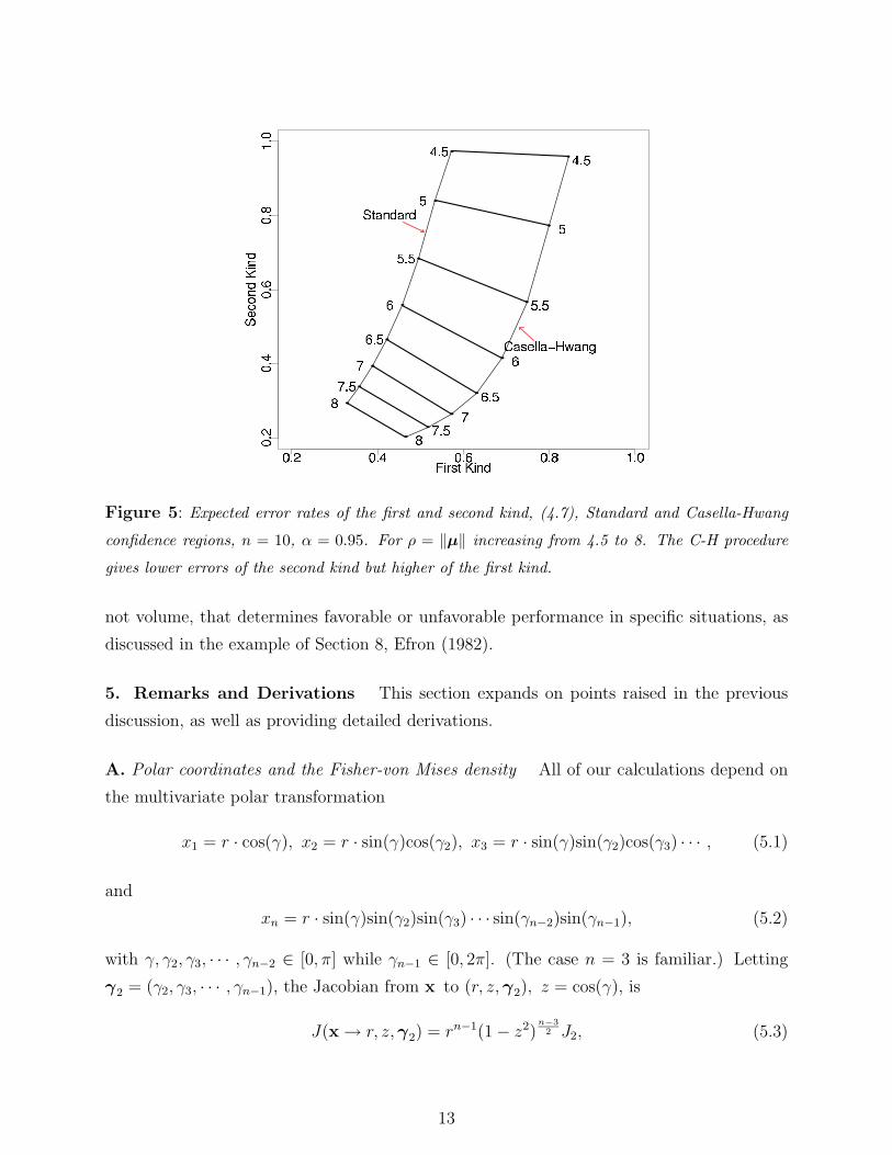
Figure 5: Expected error rates of the first and second kind, (4.7), Standard and Casella-Hwang

confidence regions, n = 10, α = 0.95. For ρ = ‖µ‖ increasing from 4.5 to 8. The C-H procedure

gives lower errors of the second kind but higher of the first kind.

not volume, that determines favorable or unfavorable performance in specific situations, as

discussed in the example of Section 8, Efron (1982).

5. Remarks and Derivations This section expands on points raised in the previous

discussion, as well as providing detailed derivations.

A. Polar coordinates and the Fisher-von Mises density All of our calculations depend on

the multivariate polar transformation

x1 = r · cos(γ), x2 = r · sin(γ)cos(γ2), x3 = r · sin(γ)sin(γ2)cos(γ3) · · · , (5.1)

and

xn = r · sin(γ)sin(γ2)sin(γ3) · · · sin(γn−2)sin(γn−1), (5.2)

with γ, γ2, γ3, · · · , γn−2 ∈ [0, π] while γn−1 ∈ [0, 2π]. (The case n = 3 is familiar.) Letting

γ2 = (γ2, γ3, · · · , γn−1), the Jacobian from x to (r, z,γ2), z = cos(γ), is

J(x → r, z,γ2) = rn−1(1 − z2)n−3

2 J2, (5.3)

13

where J2 =n−2∏j=2

sin(γj)n−1−j. The integral of J2 over the full range of γ2 equals kn, (3.9), the

(n − 2)-dimensional “area” of an (n − 1) dimensional unit sphere. (The area interpretation

of kn verifies formula (3.9) using familiar calculus methods.)

Since ‖x−µ‖2 = r2 +ρ2 −2rρz, where r = ‖x‖ and ρ = ‖µ‖, the n-dimensional normal

density of (1.1) becomes

fµ(r, z,γ2) = (2π)−n2 rn−1e−

12r2− 1

2ρ2+rρz(1 − z2)

n−32 J2 (5.4)

in polar coordinates. Integrating out γ2 gives

fµ(r, z) = (2π)−n/2knrn−1e−12r2− 1

2ρ2+rρz(1 − z2)

n−32 , (5.5)

from which the Fisher-von Mises density (2.5) for fµ(z|r) follows directly. The primary

angle γ is measured relative to µ in this argument.

Beginning with prior density g(µ) = ρ−(n−1), the same argument, interchanging the roles

of x and µ, gives

g(ρ, z|x) = g(ρ, z|r) ∝ e−ρ2/2+rρz(1 − z2)n−3

2 , (5.6)

with J(µ → ρ, z,γ2) = ρn−1(1 − z2)n−3

2 J2 canceling out the prior factor ρ−(n−1). (Here the

primary angle γ = cos−1(z) is measured relative to the fixed vector x .) Integrating out z

in (5.6) produces posterior density

g(ρ|r) =C0

crρ

e−12ρ2

[c−1rρ =

∫ 1

−1

erρz(1 − z2)n−3

2 dz

], (5.7)

as in (2.6). It can be shown that

C−10 =

∫ 1

−1

[Φ(rz)/ϕ(rz)](1 − z2)n−3

2 dz, (5.8)

where Φ and ϕ are the standard normal cdf and density.

A Bessel function expression for (2.6) appears in formula 9.6.18 of Abramowitz and

Stegun (1964), but the integral form for Crρ is more convenient for computation than the

usual Bessel power series representation.

B. The MinVolume Region The MinVol curve in Figure 4 is the inclusion function aρ(r), r =

6, that minimizes volume of the corresponding confidence region (2.12) subject to α†(r) =

14

0.95, (3.6). First we consider minimizing volume subject to the Bayesian constraint α(r) =

0.95, (3.8).

The volume and α(r) contributions from an infinitesimal interval [ρ, ρ + dρ] are

dV =

[knρn−1

∫ 1

zρ(r)

(1 − z2)n−3

2 dz

]dρ

and

dα =

[g(ρ|r)

∫ 1

zρ(r)

crρerρz(1 − z2)

n−32 dz

]dρ.

(5.9)

A small change dz in zρ(r) produces changes (dV )′ and (dα)′, with

(dα)′

(dV )′=

g(ρ|r)crρerρz

knρn−1=

c0erρz−ρ2/2

knρn−1, (5.10)

using (5.7). A standard extremal argument says that (5.10) must be a constant along the

volume-minimizing boundary zρ(r). Taking logs in (5.10) gives

zρ(r) =ρ2/2 + (n − 1) log(ρ) + λ

rρ, (5.11)

where λ is a free constant. Here we have not accounted for the constraint zρ(r) ∈ [−1, 1], but

Kuhn-Tucker calculations show that truncating (5.11) to [−1, 1] yields the correct MinVolume

solution.

Choosing different λ’s gives MinVolume regions for different choices of Bayes coverage

probability (3.8). Figure 6 shows the optimum boundaries as α(r) varies from 0.005 to 0.99.

Notice that the origin 0 is always included, as can be seen by letting ρ → 0 in (5.11). For

larger values of r the optimum region breaks into two components, one of which contains

0. As communicated in Samworth (2005), the James-Stein estimate tends to lie above the

regions’ midpoints.

Defining φρ(r) = log(g†(ρ|r)/g(ρ|r)), the same argument gives

zρ(r) =ρ2/2 + (n − 1) log(ρ) + ∂φρ(r)/∂r + λ

rρ, (5.12)

again truncated to [−1, 1], as the optimal boundary for minimizing volume subject to α†(r),

(3.6), equaling some specific value α; numerical methods are needed to solve (5.12). Figure

3 shows that φρ(r) is nearly 1 for r = 6, n = 10, and in fact the α = 0.95 boundary in Figure

6 nearly equals MinVolume in Figure 1, except near the origin. (Different horizontal scales

in the two figures distort the visual comparison.)

15

Figure 6: Bayes optimum boundary (5.11), r = 6, n = 10, for α(r), (3.8), ranging from 0.005 to

0.99. The 0.95 curve nearly equals that for MinVolume in Figure 1.

The Bayes boundary can also be derived from Neyman-Pearson considerations. Let

h1(µ) = 1 and h2(µ) = g(µ|x) = ρ−(n−1), (3.5). We wish to choose Cx to minimize V =∫Cx h1(µ)dµ subject to α =

∫Cx h2(µ)dµ. According to the Neyman-Pearson lemma, the

optimizing region is

Cx = {µ : h2(µ)/h1(µ) ≥ λα}, (5.13)

with constant λα chosen to satisfy the α constraint. Our previous results show that

h2(µ) ∝ ρ−(n−1)e−12(r2+ρ2−2rρz), (5.14)

making (5.14) equivalent to (5.11).

C. Minimum Volume Acceptance Regions Suppose that we wish to choose aρ(r) to be

the function of r that minimizes the volume of acceptance region Aµ, (2.10), subject to

constraint∫ ∞

0aρ(r)fρ(r)dr = α, α = 0.95 in Figure 2. The equivalent of relations (5.9) for

16

this situation is

dV =

[knrn−1

∫ 1

zρ(r)

(1 − z2)n−3

2 dz

]dr

and

dα =

[fρ(r)

∫ 1

zρ(r)

crρerρz(1 − z2)

n−32 dz

]dr.

(5.15)

Integrating out z from (5.5) yields a convenient expression for the non-central chi density

fρ(r),

fρ(r) = ce−ρ2/2rn−1e−r2/2/crρ

(c =

[2

n2−1√

π Γ

(n − 1

2

)]−1). (5.16)

In this case (5.10) becomes

(dα)′

(dV )′= constant · e− 1

2‖x − µ‖2

, (5.17)

showing that the standard acceptance spheres {x : ‖x − µ‖ ≤ χ(α)n } are minimum volume.

Here, as opposed to Figure 3, it is the standard inclusion function aρ(r) that is shifted

leftwards, reducing volume by reducing r, in analogy with (3.9).

D. Hierarchical Models A familiar hierarchical Bayes model for estimating µ in (1.2) takes

µ ∼ N(0, CI) where C has an improper “hyperprior” density

h(C) = C−p/2, C > 0, (5.18)

Efron and Morris (1975), Berger and Strawderman (1996). Formal integration, using polar

coordinates, gives µ marginal density

g(µ) = ρ−(n−2+p), (5.19)

so we see that the choice p = 1 results in (3.5), which we called the uninformative prior for

µ. The resulting squared error Bayes estimate of µ having observed x ∼ N(µ, I) is minimax

and admissible, Morris (private communication), Berger and Strawderman (1996).

Selecting p different from 1 in (5.18) has only minor effects on our theory, for example

changing n − 1 in (5.10)-(5.11) to n − 2 + p. The choice p = 0 makes the Bayes and James-

Stein estimates most alike; in this sense p = 1 is an “overshrinker”, which explains the

above-center location of js in Figure 6.

17

E. The Case x ∼ N(µ, σ2I), σ2 unknown In most linear model situations (1.1) is general-

ized to

x ∼ N(µ, σ2I) independent of s2 ∼ σ2χ2ν/ν. (5.20)

However the results of this paper do not extend easily to situation (5.20), at least not the

frequentist results. (Nor do those in our main references.) The difficulty here lies with the

distribution of γ, or z = cos(γ), where there is no obvious pivotal quantity that has its

density independent of the nuisance parameter σ. We might, instead, eliminate σ by giving

it some sort of objective prior. The scale invariant prior density π(σ) = σ−d produces a

version of the Fisher-von Mises density (2.5) for situation (5.20),

fµ(z|r, s) = c(1 − z2)n−3

2

∫ ∞

0

crρt2t2(v2−1/2)e(rρz−v2)t2dt (5.21)

where r = r/s, ρ = ρ/s, v2 = (v + d − 1)/2, and c = 2vv22 /Γ(v2), from which we might

construct regions as in Section 2.

F. The Casella-Hwang and Tseng-Brown Regions Let c2 equal the upper α quantile of a

χ2n variate, c2 = χ

(α)2n in (1.3), and define

R = 1 − (n − 2)/r2. (5.22)

Assuming r2 > c2 > n (satisfied in Figure 1, where r2 = 36, c2 = 18.3, n = 10), the Casella-

Hwang confidence region is a sphere centered at the James-Stein estimator R·x, with squared

radius R · (c2 − n log(R)). This radius is less than χ(α)n , the standard region radius in (1.3).

The Tseng-Brown construction is based on spherical acceptance regions,

A(µ) =

{x :

∥∥∥x − µ

(1 +

1

A + Bρ2

)∥∥∥2

≤ χ2n

(ρ2

(A + Bρ2)2

)(α)}, (5.23)

where χ2n(∆2)(α) indicates the upper α quantile of a noncentral chi-squared distribution with

noncentrality parameter ∆2. Inverting A(µ) gives oblate confidence regions, as seen in Figure

1. The constants A and B depend on n and α; with n = 10 and α = 0.95, their Table 2

provides A = 3.44, B = 0.125.

18

References

Abramowitz, M. and Stegun, L. (1968) Handbook of Mathematical Functions, National Bu-

reau of Standards, Applied Mathematics Series 55.

Berger, J. (1980) A robust generalized Bayes estimator and confidence region for a multi-

variate normal mean. Ann. Stat., 8, 716-761.

Berger, J. and Strawderman, W. (1996) “Choice of hierarchical priors: admissability in

estimation of normal means”, Ann. Stat., 24, 931-951.

Brown, L., Casella, G., and Hwang, G. (1995) “Optimal confidence sets and the Limacon of

Pascal”, JASA, 90, 880-889.

Casella, G. and Hwang, J.T. (1983) Empirical Bayes confidence sets for the mean of a

multivariate normal distribution. JASA, 78, 688-698.

Downs, T. (1966) “Some relationships among von Mises distributions of different dimen-

sions”, Biometrika, 53, 269-272.

Efron, B. and Morris, C. (1975) “Data analysis using Stein’s estimator and its competitors”,

JASA, 70, 311-319.

Efron, B. (1982) “Maximum likelihood and decision theory”, Ann. Stat., 10, 340-356.

Efron, B. (1993) “Bayes and likelihood calculations from confidence intervals”, Biometrika,

80, 3-26.

Faith, R.E. (1976) Minimax Bayes set and point estimators of a multivariate normal mean,

Technical Report 66. University of Michigan, Ann Arbor.

Peers, H. (1965) “On confidence points and Bayesian probability points in the case of several

parameters”, JRSS-B, 27, 9-16.

Robinson, G.K. (1979a) Conditional properties of statistical procedures, Ann. Stat., 7, 742-

755.

Samworth, R. (2005) “Small confidence sets for the mean of a spherically symmetric distri-

bution” JRSS-B, 67, 343-362.

Scheffe, M. (1959) The Analysis of Variance, Wiley, N.Y.

Stein, C. (1962) Confidence sets for the mean of a multivariate normal distribution (with

discussion). JRSS-B, 24, 265-296.

19

Stein, C. (1985) “On the coverage probability of confidence sets based on a prior distribu-

tion”, Banach Center Publications, 16, Warsaw: PWN-Polish Scientific Publishers.

Tibshirani, R. (1989) “Noninformative priors for one parameter of many”, Biometrika, 76,

604-608.

Tseng, Y.L. and Brown, L.D. (1997) Good exact confidence sets for a multivariate normal

mean. Ann. Stat., 25, 2228-2258.

20