Journal of Data Science 465-484 , DOI: 10.6339/JDS.201807_16(3).0002

MINIMUM PROFILE HELLINGER DISTANCE ESTIMATION FOR A

TWO-SAMPLE LOCATION-SHIFTED MODEL

Haocheng Li*1, Jingjing Wu*1, Jian Yang1

1Department of Mathematics and Statistics, University of Calgary

* These two authors contribute equally to the work

Abstract: Minimum Hellinger distance estimation (MHDE) for parametric model is

obtained by minimizing the Hellinger distance between an assumed parametric model

and a nonparametric estimation of the model. MHDE receives increasing attention for

its efficiency and robustness. Recently, it has been extended from parametric models

to semiparametric models. This manuscript considers a two-sample semiparametric

location-shifted model where two independent samples are generated from two

identical symmetric distributions with different location parameters. We propose to use

profiling technique in order to utilize the information from both samples to estimate

unknown symmetric function. With the profiled estimation of the function, we propose

a minimum profile Hellinger distance estimation (MPHDE) for the two unknown

location parameters. This MPHDE is similar to but dif- ferent from the one introduced

in Wu and Karunamuni (2015), and thus the results presented in this work is not a

trivial application of their method. The difference is due to the two-sample nature of

the model and thus we use different approaches to study its asymptotic properties such

as consistency and asymptotic normality. The efficiency and robustness properties of

the proposed MPHDE are evaluated empirically though simulation studies. A real data

from a breast cancer study is analyzed to illustrate the use of the proposed method.

Key words: Minimum Hellinger distance estimation, profiling, two-sample

location-shifted model, efficiency, robustness.

1 Introduction

Minimum distance estimation of unknown parameters in a parametric model is obtained by

minimizing the distance between a nonparametric distribution esti- mation (such as empirical, kernel,

etc) and an assumed parametric model. Some well-known examples of minimum distance estimation

include least-squares esti- mation and minimum Chi-square estimation. Among different minimum

distance estimations, minimum Hellinger distance estimation (MHDE) receives increasing attention

for its superior properties in efficiency and robustness. The idea of the estimation using Hellinger

466 MINIMUM PROFILE HELLINGER DISTANCE ESTIMATION FOR A TWO-SAMPLE LOCATION-SHIFTED MODEL

distance was firstly introduced by Beran (1977) for parametric models. Simpson (1987) examined the

MHDE for discrete data. Yang (1991) and Ying (1992) studied censored data in survival analysis by

using the MHDE. Woo and Sriram (2006) and Woo and Sriram (2007) employed the MHDE method

to investigate mixture complexity in finite mixture models. The MHDEs for mixture models were

also studied by many literatures such as Lu et al. (2003) and Xiang et al. (2008). Other applications

of the MHDE method can be referred to Takada (2009), N’drin and Hili (2013) and Prause et al.

(2016).

Recently, the MHDE method was extended to semiparametric model of gen- eral form. Wu and

Karunamuni (2009) and Wu and Karunamuni (2012) proved that MHDE retains good efficiency and

robustness properties for semiparametric model of general form under certain conditions. However,

the MHDE usually re- quires an estimate of infinite-dimensional nuisance parameter in

semiparametric models, which leads to computational difficulty. To solve this problem, Wu and

Karunamuni (2015) proposed a minimum profile Hellinger distance estimation (MPHDE). The

MPHDE method profiles out the infinite-dimensional nuisance parameter and thus circumvents the

computational obstacle. Wu and Karuna- muni (2015) derived the MPHDE for one-sample

symmetric location model, while in real applications two-sample location-shifted symmetric model is

often encoun- tered. For example, as we will show in data application section, the comparison of

biomarkers across different patient groups requires two-sample models. There- fore, in this

manuscript we extend the MPHDE approach to two-sample location- shifted symmetric model.

The idea of using profiling approach is quite intuitive but its theoretical frame- work is often

complicated to study. For one-sample case, Wu and Karunamuni (2015) used the Hellinger distance

between the location model and its nonpara- metric estimation. However, this method does not work

for our two-sample case because it cannot utilize the information for the nuisance parameter

contained in both samples. To handle the two-sample estimation, we propose a new Hellinger

distance between the location-shifted model and its estimation that involves the nuisance density

estimation and the location parameters of our interest. Conse- quently, a novel approach is proposed

to explore the asymptotic properties of the resulted estimator obtained from minimizing the new

Hellinger distance.

The remainder of this paper is organized as follows. In Section 2 we propose a MPHDE for

the two-sample semiparametric location-shifted model. Section 3 presents the asymptotic

properties of the proposed MPHDE with all proofs deferred to appendix. In Section 4, we evaluate

the performance of the MPHDE by simulation studies compared with commonly used least-squares

and maximum

likelihood estimation methods. A data from a real breast cancer study is analyzed in Section 5 to

demonstrate the use of the proposed method. Concluding remarks are given in Section 6.

Haocheng Li, Jingjing Wu, Jian Yang 467

2 MPHDE for Two-Sample Location Model

Suppose we have two samples with n0 and n1 independent and identically dis- tributed (i.i.d.)

random variables (r.v.s), respectively. Denote the two samples as𝑋𝑖, 𝑖 = 1,⋯ , 𝑛0 , and 𝑌𝑗, 𝑗 =

1,⋯ , n1. We assume that the two samples are independent and they follow

𝑋1,⋯,𝑋𝑛0 ~ⅈ.ⅈ.𝑑.𝑓

0(⋅)=𝑓(∙−𝜃0)

𝑌1,⋯,𝑌𝑛1 ~ⅈ.ⅈ.𝑑.𝑓

1(⋅)=𝑓(∙−𝜃1)

(1)

where θ = (θ0, θ1)⊤is the location parameter vector of our interest and the unknown f ∈ H is

treated as the nuisance parameter. Here H is the collection of all continuous even densities. We focus

on model (1) in this paper and work on the inference for the location parameter θ. Model (1) could be

represented in a regression form. Let total sample size be n = n0 + n1. The r.v.s in model (1) could

be written as{(𝑍𝑖, 𝐷𝑖): 𝑖 = 1,⋯ , 𝑛}, where (𝑍1, … , 𝑍𝑛)⊤ = (𝑋1,⋯ , 𝑋𝑛0 , 𝑌1, ⋯ ,⋅ 𝑌𝑛1)

⊤ and Di is an

indicator function taking Di = 1 if Zi is from f1 and 0 otherwise.Model (1) can be equivalently

represented as

𝑍𝐼̇ = 𝜃0 + (𝜃1 − 𝜃0)𝐷𝑖 + 𝜖𝑖

where the i.i.d. error terms ϵi’s are from f .

For any given θ, since X1 – θ0, . . . , Xn0 – θ0, Y1 – θ1, . . . , Yn1 − θ1 are i.i.d. r.v.s from f , we can

estimate the unknown f using the following kernel density estimator based on the pooled sample:

𝑓(𝜃；𝑥) =1

𝑛𝑏𝑛{∑𝐾[

𝑥 − (𝑋𝑖 − 𝜃0)

𝑏𝑛]

𝑛0

𝑖=1

+∑𝐾[𝑥 − (𝑌𝑖 − 𝜃1)

𝑏𝑛]

𝑛1

𝑖=1

}

=𝑛0

𝑛{

1

𝑛0𝑏𝑛∑𝐾[

𝑥 − (𝑋𝑖 − 𝜃0)

𝑏𝑛]

𝑛0

𝑖=1

+𝑛1𝑛∑𝐾[

𝑥 − (𝑌𝑖 − 𝜃1)

𝑏𝑛]

𝑛1

𝑖=1

}

= 𝜌0𝑓0(𝑥 + 𝜃0) + 𝜌1𝑓1(𝑥 + 𝜃1)

where 𝜌0 = 𝑛0/𝑛, 𝜌1 = 1 − 𝜌0 = 𝑛1/𝑛, kernel function K is a symmetric density function, the

bandwidth bn is a sequence of positive constants such that bn → 0 as n → ∞, and 𝑓0 and 𝑓1 are

kernel density estimators of f0 and f1, respectively. To be specific, f0 and f1 have

𝑓0̂(𝑥) =1

𝑛0𝑏𝑛∑ 𝐾(

𝑥−𝑋ⅈ

𝑏𝑛)

𝑛0𝑖=1 (3)

and

𝑓1̂(𝑥) =1

𝑛1𝑏𝑛∑ 𝐾(

𝑥−𝑌ⅈ

𝑏𝑛)

𝑛1𝑖=1 (4)

Even though ρ0 and ρ1 depend on n, we depress their dependence for notation simplicity. We

generally require that ni/n → ρi as n → ∞ with ρi ∈ (0, 1), i = 0, 1. Based on (2), f0 and f1 can also

be estimated respectively by

𝑓0̃(𝑥) = 𝑓(𝜃；𝑥 − 𝜃0) = 𝜌0𝑓0(𝑥) + 𝜌1𝑓1(𝑥 − 𝜃0 + 𝜃1)

and

468 MINIMUM PROFILE HELLINGER DISTANCE ESTIMATION FOR A TWO-SAMPLE LOCATION-SHIFTED MODEL

𝑓1̃(𝑥) = 𝑓(𝜃；𝑥 − 𝜃1) = 𝜌0𝑓0(𝑥 + 𝜃0 − 𝜃1) + 𝜌1𝑓1(𝑥)

To obtain the MPHDE of θ, we firstly profile the unknown nuisance parameter f out by

minimizing the sum of the squared Hellinger distance for the two samples, i.e.

𝑚𝑖𝑛𝑓∈𝐻

{||𝑓0̃

12(𝑥) − 𝑓0

12(𝑥)||

2

+ ||𝑓1̃

12(𝑥) − 𝑓1

12(𝑥)||

2

}

= 𝑚𝑖𝑛𝑓∈𝐻

{||[𝜌0𝑓0(𝑥) + 𝜌1𝑓1(𝑥 − 𝜃0 + 𝜃1)]12 − 𝑓

12(𝑥 − 𝜃0)||

2

+ ||[𝜌0𝑓0(𝑥 + 𝜃0 − 𝜃1) + 𝜌1𝑓1(𝑥)]12 − 𝑓

12(𝑥 − 𝜃1)||

2

}

= 𝑚𝑖𝑛𝑓∈𝐻

{2 ||[𝜌0𝑓0(𝑥 + 𝜃0) + 𝜌1𝑓1(𝑥 + 𝜃1)]12 − 𝑓

12(𝑥)||

2

}

= 4{1 −𝑚𝑎𝑥𝑓∈𝐻

∫[𝜌0𝑓0(𝑥 + 𝜃0) + 𝜌1𝑓1(𝑥 + 𝜃1)]12 𝑓

12(𝑥) 𝑑𝑥}

= 4 {1 −𝑚𝑎𝑥𝑓∈𝐻

∫𝑓12(𝜃；𝑥) 𝑓

12(𝑥) 𝑑𝑥}

Note that 𝑓1

2(𝜃;⋅) can be represented as

𝑓12(𝜃; 𝑥) =

1

2[𝑓12(𝜃; 𝑥) + 𝑓

12(𝜃; −𝑥)] +

1

2[𝑓12(𝜃; 𝑥) − 𝑓

12(𝜃;−𝑥)] = 𝜂1̂(𝜃; 𝑥) + 𝜂2̂(𝜃; 𝑥),

say,

where 𝜂1̂(𝜃;．) is an even function while 𝜂2̂(𝜃;．) is an odd function. As a result,

∫𝑓12(𝜃；𝑥) 𝑓

12(𝑥) 𝑑𝑥 = ∫[𝜂1̂(𝜃; 𝑥) + 𝜂2̂(𝜃; 𝑥)]𝑓

12(𝑥) 𝑑𝑥 = ∫𝜂1̂(𝜃; 𝑥)𝑓

12(𝑥) 𝑑𝑥

By the Cauchy-Schwarz inequality, ∫𝜂1̂(𝜃; 𝑥)𝑓1

2(𝑥) 𝑑𝑥 is uniquely maximized by

𝑓1

2(𝑥) = 𝜂1̂(𝜃; 𝑥)/‖𝜂1̂(𝜃; 𝑥)‖ and thus 𝑓1

2(𝑥) = 𝜂1̂2(𝜃; 𝑥)/‖𝜂1̂(𝜃; 𝑥)‖

2 is the profiled f .

Therefore, after replacing 𝑓1

2(𝑥) with 𝜂1̂(𝜃; 𝑥)/‖𝜂1̂(𝜃; 𝑥)‖, the MPHDE 𝜃 of θ is given by

𝜃 = 𝑎𝑟𝑔 𝑚𝑎𝑥𝑡=(𝑡0,𝑡1)

⊤∈ℝ2∫𝜂1̂(𝑡; 𝑥)

𝜂1̂(𝑡;𝑥)

‖𝜂1̂(𝑡;𝑥)‖𝑑𝑥

= 𝑎𝑟𝑔 𝑚𝑎𝑥𝑡∈ℝ2

‖𝜂1̂(𝑡; 𝑥)‖

= 𝑎𝑟𝑔 𝑚𝑎𝑥𝑡∈ℝ2

‖𝑓1

2(𝑡; 𝑥) + 𝑓1

2(𝑡; −𝑥)‖ (5)

= 𝑎𝑟𝑔 𝑚𝑎𝑥𝑡∈ℝ2

∫[𝜌0𝑓0(𝑥 + 𝑡0) + 𝜌1𝑓1(𝑥 + 𝑡1)]12[𝜌0𝑓0(−𝑥 + 𝑡0) + 𝜌1𝑓1(−𝑥 + 𝑡1)]

12 𝑑𝑥

= 𝑎𝑟𝑔 𝑚𝑖𝑛𝑡∈ℝ2

‖𝑓1

2(𝑡; 𝑥) − 𝑓1

2(𝑡;−𝑥)‖

Haocheng Li, Jingjing Wu, Jian Yang 469

= : 𝑇(𝑓0, 𝑓1)

where in the last equality we represent 𝜃 as a functional T which only depends on 𝑓0 and 𝑓1.

As there is no explicit expression of the solution to the above optimization in (5), 𝜃 has to be

calculated numerically. In this manuscript, the computation was implemented by the R function “nlm”

with the medians of Xi and Yi to be the initial values of 𝜃0 and 𝜃1, respectively. The numerical

optimization leads to satisfactory results in our simulation and data application studies. All of them

successfully achieve convergence.

Remark 1. Even though θ can take any value in ℝ2, we can use a large enough compact subset

of ℝ2, say Θ = [−A, A]2 with A to be a large positive number, so that θ is an interior point of Θ, i.e.

θ ∈ int(Θ). Thus in what follows we will optimize θ over Θ instead of ℝ2 simply for technical

convenience.

Remark 2. The proposed MPHDE involves the mixture model 𝜌0𝑓(．− 𝜃0) + 𝜌1𝑓(．− 𝜃1)

which has been studied by many literatures such as ecently Xi- ang et al. (2014), Erisoglu and

Erisoglu (2013), and Ngatchou-Wandji and Bulla(2013). For the identifiability of this model, we can

assume θ0 < θ1 without any loss of generality. By Theorem 2 of Hunter et al. (2007), this mixture

model is identifiable if ρ0 ∈ (0, 0.5) ∪ (0.5, 1). If f is unimodal, then this mixture model is

identifiable even when ρ0 = 0.5. Therefore the identifiability is not a problem for the MPHDE and we

will assume from now on that the mixture model is identifiable for the sake of simplicity.

Remark 3. For one-sample location model 𝑓(．− 𝜃), the Hellinger distance is between the

location model, involving both f and θ together, and its nonparametric estimation. For this

two-sample model, in order to use the information about the nuisance parameter f contained in both

the first and second samples, the Hellinger distance is between f and its estimation that involves the

nuisance density estimation and the location parameters of our interest.

3 Asymptotic Properties

In this section, we discuss the asymptotic distribution of the MPHDE 𝜃 given in (5) for the

two-sample semiparametric location-shifted model (1). Note that 𝜃 given in (5) is a bit different

than the MPHDE defined in Wu and Karunamuni (2015) for general semiparametric models in the

sense that the former incorpo- rates the model assumption in the nonparametric estimation of f while

the later uses a completely nonparametric estimation of f not depending on the model at all. In this

sense, we can not apply the asymptotics obtained in Wu and Karuna- muni (2015) to our model (1).

Instead we will directly derive below the existence,consistency and asymptotic normality of 𝜃. Let F

be the set of all densities with respect to (w.r.t.) Lebesgue measure on the real line. We first give in

the next theorem the existence and uniqueness of the MPHDE 𝜃.

Theorem 1. Suppose that T is defined by (5). Then,

(i) For any g0, g1 ∈ F, there exists T (g0, g1) satisfying (5).

470 MINIMUM PROFILE HELLINGER DISTANCE ESTIMATION FOR A TWO-SAMPLE LOCATION-SHIFTED MODEL

(ii) If T (g0, g1) is unique, then T is continuous at (𝑔0, 𝑔1)⊤ in the Hellinger metric. In another

word, T (gn0, gn1) → T (g0, g1) for any sequences gn0 and gn1 such that ‖𝑔𝑛𝑖1/2 − 𝑔𝑖

1/2‖ → 0 as

n → ∞, i = 0, 1.

(iii) The MPHDE is Fisher-consistent, i.e. T (f0, f1) = θ uniquely for every (𝑓0,𝑓1)⊤

satisfying model (1).

The following theorem is a consequence of Theorem 1 which gives the consis- tency of the

MPHDE 𝜃 defined in (5).

Theorem 2. Suppose that the kernel K in (3) and (4) are absolutely continuous, has compact

support and bounded first derivative, and the bandwidth bn satisfies bn → 0 and 𝑛1/2𝑏𝑛 → ∞ as

n → ∞. If f in model (1) is uniformly continuous on its support, then ‖𝑓𝑖1/2

− 𝑓𝑖1/2‖

𝑝→ 0, i = 0, 1,

and furthermore the MPHDE 𝜃𝑝→ 𝜃.

The next Theorem 3 gives the expression of the different 𝜃 − 𝜃 which will be used to establish

the asymptotic normality of θˆ in Theorem 4.

Theorem 3. Assume that the conditions in Theorem 2 are satisfied. Further suppose f has

uniformly continuous first derivative. Then

∑ (𝜃 − 𝜃)1 = −(𝜌0𝜌1) [𝜌0 ∫

𝑓′

𝑓(𝑥) 𝑓0(𝑥 + 𝜃0) 𝑑𝑥 + 𝜌1 ∫

𝑓′

𝑓(𝑥) 𝑓1(𝑥 + 𝜃1) 𝑑𝑥] ∙ (1 + 𝑜𝑝(1)), (6)

where

∑ =1(𝜌0

2 𝜌0𝜌1𝜌0𝜌1 𝜌1

2 )∫(𝑓′)2

𝑓(𝑥) 𝑑𝑥 − (

𝜌0 00 𝜌0

)∫𝑓′′(𝑥)𝑑𝑥

With (6) and some regularity condition we can immediately derive the asymptotic distribution of

𝜃 − 𝜃 given in the next theorem.

Theorem 4. Assume that the conditions in Theorem 3 are satisfied and in addition f has

continuous third derivative, ∫𝑓′′(𝑥) 𝑑𝑥 ≠ ∫(𝑓′)2

𝑓(𝑥) 𝑑𝑥 and the bandwidth satisfies 𝑛𝑏6𝑛 → 0 as

n → ∞. Then the asymptotic distribution of √𝑛(𝜃 − 𝜃) is N (0, Σ) with covariance matrix Σ defined

by

∑=

{

∫

(𝑓′)2

𝑓𝑑𝑥 𝛴1

−1 (𝜌0

2 𝜌0𝜌1𝜌0𝜌1 𝜌1

2 )𝛴1−1, 𝑖𝑓 ∫𝑓′′(𝑥) 𝑑𝑥 ≠ 0

[∫(𝑓′)2

𝑓𝑑𝑥]−1 (

1/𝜌0 00 1/𝜌0

) , 𝑖𝑓 ∫ 𝑓′′(𝑥) 𝑑𝑥 = 0

Remark 3. Distributions satisfying ∫𝑓′′(𝑥) 𝑑𝑥 = 0 include those with support on the whole real

line, such as normal and t distributions. The distributions satisfying ∫𝑓′′(𝑥) 𝑑𝑥 ≠ 0 include those

with finite support and its first derivative evaluated at boundary of support is non-zero, such as

f(x) =3

4(1 − 𝑥2)𝑓𝑜𝑟|𝑥| ≤ 1.

Haocheng Li, Jingjing Wu, Jian Yang 471

Remark 4. If the two samples in (1) are actually a single sample from the mixture 𝜌0𝑓(∙ −𝜃0) +

𝜌1𝑓(∙ −𝜃1) with known classification for each data point, then by comparing the lower bound of

asymptotic variance described in Wu and Karunamuni (2015) with the results in our Theorem 4, we

can conclude that the proposed MPHDE 𝜃 defined in (5) is efficient, in the semiparametric sense,

for any f . In addition, if ∫𝑓′′(𝑥) 𝑑𝑥 = 0 , then this semiparametric model is an adaptive model and

the proposed MPHDE 𝜃 is an adaptive estimator.

4 Simulation Studies

We assess the empirical performance of the proposed MPHDE in Section 2 for the two-sample

location-shifted model. Five hundred simulations are run for each parameter configuration. We

consider a parameter setting of (𝜃0, 𝜃1)⊤ = (0,1)⊤ and simulate four different distributions for f (x):

normal, Student’s t, triangular and Laplace. We set the standard deviation to be 1 for normal

distribution, the degrees of freedom to be 4 for t distribution. The triangular distribution has density

function

𝑓(𝑥) =𝑐 − |𝑥|

𝑐2, |𝑥| ≤ 𝑐,

and we set c = 1. The Laplace distribution has density function

𝑓(𝑥) =1

2𝑏𝑒𝑥𝑝 (−

|𝑥|

𝑏),

and we set b = 1. The bandwidth bn is chosen to be bn = 𝑛−1/5according to the bandwidth

requirement in Theorem 4. The biweight kernel 𝐾(𝑡) =15

16(1 − 𝑡2)2for |t| ≤ 1 is employed in the

simulation studies. We consider both smaller sample sizes n0 = n1 = 20 and larger sample sizes n0 =

n1 = 50.

As a comparison, we also give both least-squares estimation (LSE) and max- imum likelihood

estimation (MLE). For the two-sample location-shifted model (1) under our consideration, simple

calculation shows that the LSEs of θ0 and θ1 are essentially the sample means �̅� and �̅� respectively.

With f assumed known, straight calculation says that the MLEs of θ0 and θ1 are sample means for

normal case and sample medians for Laplace case, while there is no explicit expression of the MLEs

for Student’s t and Triangular populations. Tables 1 and 2 display the simulation results of MPHDE,

LSE and MLE methods for sample sizes n0 = n1 = 20 and n0 = n1 = 50, respectively. In the tables,

the term Bias represents the average of biases over the 500 repetitions; the terms RMSE and SE are

the average of root mean squared errors and empirical standard errors, respectively; and the term CR

represents the empirical coverage rate for 95% confidence intervals. From Tables 1 and 2 we can see

that all the three estimation approaches have fairly small bias. In terms of standard errors, the

MPHDE has worse performance than the LSE and the MLE regardless of sample size.

To investigate the robustness properties of the proposed MPHDE and make comparison, we

472 MINIMUM PROFILE HELLINGER DISTANCE ESTIMATION FOR A TWO-SAMPLE LOCATION-SHIFTED MODEL

examine the performance of the three methods under data con- tamination. In this simulation, the

data from model (1) is intentionally contami- nated by a single outlying observation. This is

implemented, say for n0 = n1 = 20,by replacing the last observation X20 with an integer number z

varying from −20 and 20. To quantify the robustness, the α-influence function (α-IF) discussed by Lu

et al. (2003) is used. The α-IF for parameter θi, i = 0, 1, is defined as

𝐼𝐹(𝑧) = 𝑛𝑖(𝜃𝑖𝑧 − 𝜃𝑖),

where 𝜃𝑖𝑧 represents the estimate based on the contaminated data with outlying observation

X20 = z and 𝜃𝑖 denotes the estimate based on the uncontaminated

Table 1: Simulation results for n0 = n1 = 20.

MPHDE Bias(θ0) RMSE(θ0) SE(θ0) CR(θ0) Bias(θ1) RSME(θ1) SE(θ1) CR(θ1)

Normal -0.025 0.307 0.331 0.924 -0.012 0.325 0.341 0.948

Student’s t -0.008 0.350 0.380 0.936 -0.025 0.340 0.389 0.946

Triangular 0.002 0.115 0.115 0.918 -0.005 0.114 0.115 0.918

Laplace 0.006 0.310 0.343 0.952 -0.024 0.297 0.344 0.964

LSE Bias(θ0) RMSE(θ0) SE(θ0) CR(θ0) Bias(θ1) RSME(θ1) SE(θ1) CR(θ1)

Normal -0.001 0.234 0.213 0.944 -0.005 0.229 0.214 0.926

Student’s t -0.014 0.312 0.298 0.944 -0.030 0.319 0.299 0.930

Triangular -0.0001 0.095 0.088 0.914 -0.002 0.095 0.088 0.910

Laplace -0.004 0.332 0.298 0.916 -0.002 0.327 0.298 0.916

MLE Bias(θ0) RMSE(θ0) SE(θ0) CR(θ0) Bias(θ1) RSME(θ1) SE(θ1) CR(θ1)

Normal -0.001 0.234 0.213 0.944 -0.005 0.229 0.214 0.926

Student’s t -0.011 0.266 0.292 0.950 -0.030 0.277 0.293 0.958

Triangular -0.001 0.107 0.106 0.928 -0.008 0.102 0.105 0.916

Laplace -0.0009 0.274 0.287 0.932 -0.023 0.257 0.287 0.950

Haocheng Li, Jingjing Wu, Jian Yang 473

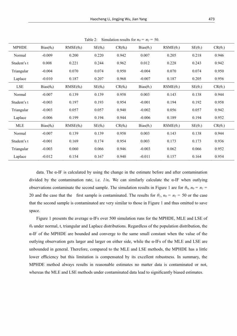
Table 2: Simulation results for n0 = n1 = 50.

MPHDE Bias(θ0) RMSE(θ0) SE(θ0) CR(θ0) Bias(θ1) RSME(θ1) SE(θ1) CR(θ1)

Normal -0.009 0.200 0.220 0.942 0.007 0.205 0.218 0.946

Student’s t 0.008 0.221 0.244 0.962 0.012 0.228 0.243 0.942

Triangular -0.004 0.070 0.074 0.950 -0.004 0.070 0.074 0.950

Laplace -0.010 0.187 0.207 0.968 -0.007 0.187 0.205 0.956

LSE Bias(θ0) RMSE(θ0) SE(θ0) CR(θ0) Bias(θ1) RSME(θ1) SE(θ1) CR(θ1)

Normal -0.007 0.139 0.139 0.958 0.003 0.143 0.138 0.944

Student’s t -0.003 0.197 0.193 0.954 -0.001 0.194 0.192 0.958

Triangular -0.003 0.057 0.057 0.940 -0.002 0.056 0.057 0.942

Laplace -0.006 0.199 0.194 0.944 -0.006 0.189 0.194 0.952

MLE Bias(θ0) RMSE(θ0) SE(θ0) CR(θ0) Bias(θ1) RSME(θ1) SE(θ1) CR(θ1)

Normal -0.007 0.139 0.139 0.958 0.003 0.143 0.138 0.944

Student’s t -0.001 0.169 0.174 0.954 0.003 0.173 0.173 0.936

Triangular -0.003 0.060 0.066 0.946 -0.003 0.062 0.066 0.952

Laplace -0.012 0.154 0.167 0.940 -0.011 0.157 0.164 0.954

data. The α-IF is calculated by using the change in the estimate before and after contamination

divided by the contamination rate, i.e. 1/ni. We can similarly calculate the α-IF when outlying

observations contaminate the second sample. The simulation results in Figure 1 are for θ0, n0 = n1 =

20 and the case that the first sample is contaminated. The results for θ1, n0 = n1 = 50 or the case

that the second sample is contaminated are very similar to those in Figure 1 and thus omitted to save

space.

Figure 1 presents the average α-IFs over 500 simulation runs for the MPHDE, MLE and LSE of

θ0 under normal, t, triangular and Laplace distributions. Regardless of the population distribution, the

α-IF of the MPHDE are bounded and converge to the same small constant when the value of the

outlying observation gets larger and larger on either side, while the α-IFs of the MLE and LSE are

unbounded in general. Therefore, compared to the MLE and LSE methods, the MPHDE has a little

lower efficiency but this limitation is compensated by its excellent robustness. In summary, the

MPHDE method always results in reasonable estimates no matter data is contaminated or not,

whereas the MLE and LSE methods under contaminated data lead to significantly biased estimates.

474 MINIMUM PROFILE HELLINGER DISTANCE ESTIMATION FOR A TWO-SAMPLE LOCATION-SHIFTED MODEL

5 Data Applications

In this section, we demonstrate the use of the proposed MPHDE method through analyzing a

breast cancer data collected in Calgary, Canada (Feng et al., 2016). Breast cancer is regarded as the

most common cancer and the second leading cause of cancer death for females in North America.

Existing studies suggest that it would be more informative to use some protein expression levels as

indicators of biological behavior (Feng et al., 2015). These biomarkers could reflect genetic

properties in cancer formation and cancer aggressiveness. Our dataset has 316 patients diagnosed

with breast cancer between years 1985 and 2000. Two interested biomarkers measured on these

patients are Ataxia telangiectasia mutated (ATM) and Ki67. ATM is a protein to support maintaining

genomic stability. Comparing with normal breast tissue, ATM could be significantly reduced in the

tissue with breast cancer. Ki67 is a protein expressed exclusively in proliferating cells. It is often

used as a prognostic marker in breast cancer.

Let 𝜃(1)and 𝜃(2) denote the location parameters in the distributions of the protein expression

level of ATM and Ki67 biomarkers, respectively. Our research focuses on the comparison of the

protein expression levels across both cancer stages (Stage) and lymph node (LN). As for cancer stage,

𝜃0(𝑘)

and 𝜃1(𝑘)

(k = 1, 2) denote the location parameters in the distributions of protein expression

level for Stage I and Stage II/III patients, respectively. Regarding LN status, 𝜃0(𝑘)

and 𝜃1(𝑘) (k = 1,

2) denote the location parameters in the distributions of protein expression level for negative LN

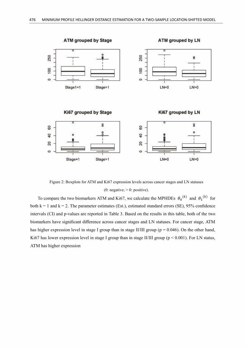
(LN-) and positive LN (LN+) patients, respectively. Figure 2 displays the boxplots for ATM

and Ki67 expression levels across both cancer stages and LN statuses, respectively. From this figure

we do see the difference in location of both ATM and Ki67 variables across both cancer stages and

LN statuses, especially for Ki67 considering the smaller variation in expression level.

Haocheng Li, Jingjing Wu, Jian Yang 475

(a) Normal (b) Student’s t

(c) Triangular (d) Laplace

Figure 1: The average α-IFs under (a) normal distribution, (b) Student’s t dis- tribution, (c) triangular

distribution and (d) Laplace distribution. Thin-solid line represents the zero horizontal baseline, and the

thick-solid, dot-dashed and dashed lines represent respectively the MPHDE, LSE and MLE approaches.

476 MINIMUM PROFILE HELLINGER DISTANCE ESTIMATION FOR A TWO-SAMPLE LOCATION-SHIFTED MODEL

Figure 2: Boxplots for ATM and Ki67 expression levels across cancer stages and LN statuses

(0: negative; > 0: positive).

To compare the two biomarkers ATM and Ki67, we calculate the MPHDEs 𝜃0(𝑘)

and 𝜃1(𝑘)

for

both k = 1 and k = 2. The parameter estimates (Est.), estimated standard errors (SE), 95% confidence

intervals (CI) and p-values are reported in Table 3. Based on the results in this table, both of the two

biomarkers have significant difference across cancer stages and LN statuses. For cancer stage, ATM

has higher expression level in stage I group than in stage II/III group (p = 0.046). On the other hand,

Ki67 has lower expression level in stage I group than in stage II/III group (p < 0.001). For LN status,

ATM has higher expression

Haocheng Li, Jingjing Wu, Jian Yang 477

Table 3: Breast cancer data analysis results based on MPHDE.

Cancer Stage

Biomarker Group Est. SE 95%CI p-value

ATM I �̂�0(1)

90.35 (73.33,107.37) 0.046

ATM II/III �̂�1(1)

68.11 (54.39,81.84)

Ki67 I �̂�0(2)

6.29 (5.05,7.53) <0.001

Ki67 II/III �̂�1(2)

8.63 (5.55,11.70)

Lymph node(LN)Status

Biomarker Group Est. SE 95%CI p-value

ATM LN－ �̂�0(1)

95.89 (76.92, 114.87) 0.019

ATM LN＋ �̂�1(1)

70.17 (60.10,80.25)

Ki67 LN－ �̂�0(2)

6.82 (6.13,7.49) <0.001

Ki67 LN＋ �̂�1(2)

10.02 (5.20,14.81)

level in negative LN group than in positive LN group (p = 0.019), while Ki67 has lower

expression level in negative LN group than in positive LN group (p < 0.001).

6 Concluding Remarks

In this paper, we propose to use MPHDE for the inferences of the two-sample semiparametric

location-shifted model. Compared with commonly used least- squares and maximum likelihood

approaches, the proposed method leads to ro- bust inferences. Simulation results demonstrate

satisfactory performance and the analysis for the breast cancer data exemplifies its utility in real

practice.

Acknowledgments

The authors thank Dr. Xiaolan Feng for providing the breast cancer data. This research was

supported by the Natural Sciences and Engineering Research Coun- cil of Canada (Haocheng Li,

RGPIN-2015-04409; Jingjing Wu, RGPIN-355970- 2013).

478 MINIMUM PROFILE HELLINGER DISTANCE ESTIMATION FOR A TWO-SAMPLE LOCATION-SHIFTED MODEL

Appendix

The proofs of Theorems 1, 2, 3 and 4 are presented in this section. The techniques used in the

proofs are similar to those in Karunamuni and Wu (2009).

A1. Proof of Theorem 1. (i) With 𝑡 = (𝑡0,𝑡1)⊤, define d(t) = ‖[𝜌0𝑔0(𝑥 + 𝑡0) + 𝜌1𝑔1(𝑥 +

𝑡1)]1/2 + [𝜌0𝑔0(−𝑥 + 𝑡0) + 𝜌1𝑔1(−𝑥 + 𝑡1)]

1/2‖. For any sequence 𝑡𝑛 = (𝑡𝑛0,𝑡𝑛1)⊤ such that

tn → t as n → ∞,

|𝑑(𝑡𝑛) − 𝑑(𝑡)|

≤ ‖[𝜌0𝑔0(𝑥 + 𝑡𝑛0) + 𝜌1𝑔1(𝑥 + 𝑡𝑛1)]12 + [𝜌0𝑔0(−𝑥 + 𝑡𝑛0) + 𝜌1𝑔1(−𝑥 + 𝑡𝑛1)]

12

− [𝜌0𝑔0(𝑥 + 𝑡0) + 𝜌1𝑔1(𝑥 + 𝑡1)]12 − [𝜌0𝑔0(−𝑥 + 𝑡0) + 𝜌1𝑔1(−𝑥 + 𝑡1)]

12‖

≤ ‖[𝜌0𝑔0(𝑥 + 𝑡𝑛0) + 𝜌1𝑔1(𝑥 + 𝑡𝑛1)]12 − [𝜌0𝑔0(𝑥 + 𝑡0) + 𝜌1𝑔1(𝑥 + 𝑡1)]

12‖

+ ‖[𝜌0𝑔0(−𝑥 + 𝑡𝑛0) + 𝜌1𝑔1(−𝑥 + 𝑡𝑛1)]12 − [𝜌0𝑔0(−𝑥 + 𝑡0) + 𝜌1𝑔1(−𝑥 + 𝑡1)]

12‖

≤ 2 {𝜌0∫|𝑔0(𝑥 + 𝑡𝑛0) − 𝑔0(𝑥 + 𝑡0)| 𝑑𝑥 + 𝜌1∫|𝑔1(𝑥 + 𝑡𝑛1) − 𝑔1(𝑥 + 𝑡1)| 𝑑𝑥}

12

2 {𝜌0∫|𝑔0(𝑥 + 𝑡𝑛0) − 𝑔0(𝑥 + 𝑡𝑛0 − 𝑡0)| 𝑑𝑥 + 𝜌1∫|𝑔1(𝑥 + 𝑡𝑛1) − 𝑔1(𝑥 + 𝑡𝑛1 − 𝑡1)| 𝑑𝑥}

12.

Since ∫𝑔0(𝑥) 𝑑𝑥 = ∫𝑔0(𝑥 + 𝑡𝑛0 − 𝑡0) 𝑑𝑥 = 1 , ∫[𝑔0(𝑥) − 𝑔0(𝑥 + 𝑡𝑛0 − 𝑡0)]+ 𝑑𝑥 =

∫[𝑔0(𝑥) − 𝑔0(𝑥 + 𝑡𝑛0 − 𝑡0)]− 𝑑𝑥 . Thus ∫|𝑔0(𝑥) − 𝑔0(𝑥 + 𝑡𝑛0 − 𝑡0)| 𝑑𝑥 = 2∫[𝑔0(𝑥) −

𝑔0(𝑥 + 𝑡𝑛0 − 𝑡0)]+ 𝑑𝑥. We also have |𝑔0(𝑥) − 𝑔0(𝑥 + 𝑡𝑛0 − 𝑡0)|

+ ≤ 𝑔0(𝑥), thus by the Dominated

Convergence Theorem ∫|𝑔0(𝑥) − 𝑔0(𝑥 + 𝑡𝑛0 − 𝑡0)| 𝑑𝑥 → 0 as n → ∞. Similarly ∫|𝑔1(𝑥 +

𝑡𝑛1) − 𝑔1(𝑥 + 𝑡𝑛1 − 𝑡1)| 𝑑𝑥 → 0. Therefore 𝑑(𝑡𝑛) → 𝑑(𝑡) 𝑎𝑠 𝑛 → ∞, i.e. d(t) is continuous in t

and then the maximum can be achieved over Θ.

(ii) Define dn(t) = ‖[𝜌0𝑔𝑛0(𝑥 + 𝑡0) + 𝜌1𝑔𝑛1(𝑥 + 𝑡1)]1/2 + [𝜌0𝑔𝑛0(−𝑥 + 𝑡0) + 𝜌1𝑔𝑛1(−𝑥 +

𝑡1)]1/2‖ and write 𝜃𝑛 = 𝑇(𝑔𝑛0, 𝑔1) and 𝜃 = 𝑇(𝑔𝑛0, 𝑔1). Then by similar argument as in (i),

|𝑑𝑛(𝑡) − 𝑑(𝑡)| ≤ 2 {𝜌0∫|𝑔𝑛0(𝑥) − 𝑔0(𝑥)| 𝑑𝑥 + 𝜌1∫|𝑔𝑛1(𝑥) − 𝑔1(𝑥)| 𝑑𝑥}

12.

By Hӧlder’s inequality, ∫|𝑔𝑛0(𝑥) − 𝑔0(𝑥)| 𝑑𝑥 ≤ ‖𝑔𝑛01/2 + 𝑔0

1/2‖ ∙ ‖𝑔𝑛01/2 − 𝑔0

1/2‖ ≤

4‖𝑔𝑛01/2 − 𝑔0

1/2‖ . Similarly ∫|𝑔𝑛1(𝑥) − 𝑔1(𝑥)| 𝑑𝑥 → 0, and thus supt |dn(t) −d(t)| → 0. This

implies dn(θ) − d(θ) → 0 and dn(θn) − d(θn) → 0. If 𝜃𝑛 ≠ 𝜃, then the compactness of Θ ensures that

there exists a subsequence {θm} ⊆ {θn} such that θm → θ′ ≠ θ, implying θ′ ∈ Θ and d(θm) → d(θ′) by

continuity of d from (i). From above results, we have dm(θm) – dm(θ) → d(θ′) − d(θ). By the definition

of θm, dm(θm) – dm(θ) ≥ 0. Hence, d(θ′) − d(θ) ≥ 0. But by the definition of θ and its uniqueness, d(θ)

> d(θ′). This is a contradiction. Therefore, θn → θ.

Haocheng Li, Jingjing Wu, Jian Yang 479

(iii) For (𝑓0,𝑓1)⊤ satisfying model (1),

𝑇(𝑓0, 𝑓1) = 𝑎𝑟𝑔 𝑚𝑖𝑛𝑡∈𝛩

||[𝜌0𝑓(𝑥 − 𝜃0 + 𝑡0) + 𝜌1𝑓(𝑥 − 𝜃1 + 𝑡1)]12

− [𝜌0𝑓(−𝑥 − 𝜃0 + 𝑡0) + 𝜌1𝑓(−𝑥 − 𝜃1 + 𝑡1)]12||.

By the symmetry of f and the identifiability of 𝜌0𝑓(∙ −𝜃0) + 𝜌1𝑓(∙ −𝜃1) , the minimum is

achieved when θi – ti = −θi + ti, i.e. ti = θi for i = 0, 1. Thus 𝑇(𝑓0, 𝑓1) = 𝜃.

A2. Proof of Theorem 2. If we can prove that ‖𝑓𝑖

1

2 − 𝑓𝑖

1

2‖𝑝→ 0 𝑎𝑠 𝑛 → ∞, i = 0, 1, then by (ii)

and (iii) of Theorem 1, 𝑇(𝑓0̂, 𝑓1̂)𝑝→ 𝑇(𝑓0, 𝑓1), i.e.𝜃

𝑝→ 𝜃. It is easy to show that 𝑠𝑢𝑝𝑥|𝑓0̂(𝑥) − 𝑓0(𝑥)|

𝑝→0. Note that ‖𝑓0

1

2 − 𝑓0

1

2‖

2

≤ ∫ |𝑓0(𝑥) − 𝑓0̂(𝑥)|𝑑𝑥 by the same technique used in the proof of

Theorem 1 (i) and Dominated Convergence Theorem we have ∫ |𝑓0(𝑥) − 𝑓0̂(𝑥)|𝑑𝑥𝑝→0 and thus

‖𝑓0

1

2 − 𝑓0

1

2‖

2𝑝→0. Similarly ‖𝑓1

1

2 − 𝑓1

1

2‖

2𝑝→0.

A3. Proof of Theorem 3. By Theorem 2, 𝜃 → 𝜃 𝑎𝑠 𝑛 → ∞. Thus for large n, 𝜃 ∈ int(Θ) since

θ ∈ int(Θ). Denote ℎ𝑡(𝑥) = 𝜌𝑜𝑓0(𝑥 + 𝑡0) + 𝜌1𝑓1(𝑥 + 𝑡1) , ℎ̂𝑡(𝑥) = 𝜌𝑜𝑓0(𝑥 + 𝑡0) + 𝜌1𝑓1(𝑥 +

𝑡1), 𝑠𝑡 = ℎ𝑡1/2

and �̂�𝑡 = ℎ̂𝑡1/2

. Note that hθ = f . We claim that for any t ∈ int(Θ) , any 2 × 1 real

vector e of unit euclidean length and any scalar ϵ close to zero,

𝑠𝑡+𝜖𝑒(𝑥) = 𝑠𝑡(𝑥) + 𝜖𝑒⊤�̇�𝑡(𝑥) + 𝜖𝑒

⊤𝑢𝜖(𝑥) (A.1)

and

�̇�𝑡+𝜖𝑒(𝑥) = �̇�𝑡(𝑥) + 𝜖�̈�𝑡(𝑥)𝑒 + 𝜖𝑣𝜖(𝑥)𝑒 (A.2)

hold for both 𝑠𝑡 and �̂�𝑡 , where �̇�𝑡 = 𝜕𝑠𝑡

𝜕𝑡 and �̈�𝑡 =

𝜕2𝑠𝑡

𝜕𝑡2 with components in L2, and the

components of 𝑢𝜖 and 𝑣𝜖 individually tend to zero in L2 as ϵ → 0. The proof of this statement is

shown at the end of this proof. (A.1) yields that

𝑙𝑖𝑚𝜖→0

𝜖−1∫[ℎ̂𝑡+𝜖𝑒

12(𝑥)ℎ̂𝑡+𝜖𝑒

12(−𝑥) − ℎ̂𝑡

12(𝑥)ℎ̂𝑡

12(−𝑥)]𝑑𝑥

= ∫[𝑒⊤�̇̂�𝑡(𝑥)�̂�𝑡(−𝑥) + 𝑒⊤�̇̂�𝑡(−𝑥)�̂�𝑡(𝑥)] 𝑑𝑥

= 2𝑒⊤∫ �̇̂�𝑡(𝑥)�̂�𝑡(−𝑥)𝑑𝑥

Since 𝜃 is the optimizer defined in (5), we have ∫ �̇̂��̂�(𝑥)�̂��̂�(−𝑥) 𝑑𝑥 = 0 .

Similarly ∫ �̇�𝜃(𝑥)𝑠𝜃(−𝑥) 𝑑𝑥 = 0 , ∫𝜕ℎ̂𝑡

𝜕𝑡(𝑥) 𝑑𝑥 =

𝜕

𝜕𝑡∫ ℎ̂𝑡(𝑥) 𝑑𝑥 = 0 and ∫

𝜕ℎ𝑡

𝜕𝑡(𝑥) 𝑑𝑥 =

𝜕

𝜕𝑡∫ℎ𝑡(𝑥) 𝑑𝑥 = 0 for any t ∈ int(Θ). Thus (A.1) and (A.2) give

0 = 2∫ �̇̂��̂�(𝑥)�̂��̂�(−𝑥) 𝑑𝑥

480 MINIMUM PROFILE HELLINGER DISTANCE ESTIMATION FOR A TWO-SAMPLE LOCATION-SHIFTED MODEL

= 2∫[�̇̂�𝜃(𝑥)�̂�𝜃(−𝑥) + (𝜃 − 𝜃)⊤�̇̂�𝜃(−𝑥)�̂�𝜃(𝑥) + �̈̂�𝜃(𝑥)(𝜃 − 𝜃)�̂�𝜃(−𝑥)]𝑑𝑥 + 𝑜𝑝(𝜃 − 𝜃)

= 2∫ �̇̂�𝜃(𝑥)�̂�𝜃(−𝑥)𝑑𝑥 + 2∫[�̇̂�𝜃(−𝑥)�̇̂�𝜃⊤(𝑥) + �̂�𝜃(−𝑥)�̈̂�𝜃(𝑥)] 𝑑𝑥 (𝜃 − 𝜃) + 𝑜𝑝(𝜃 − 𝜃)

(A.3)

Since 𝑓0 → 𝑓0 and𝑓1 → 𝑓1 uniformly by the proof of Theorem 2,

−2∫[�̇̂�𝜃(−𝑥)�̇̂�𝜃⊤(𝑥) + �̂�𝜃(−𝑥)�̈̂�𝜃(𝑥)]𝑑𝑥

= −2∫[�̇̂�𝜃(−𝑥)�̇̂�𝜃⊤(𝑥) + �̂�𝜃(−𝑥)�̈̂�𝜃(𝑥)]𝑑𝑥 + 𝑜𝑝(1)

= −2∫{1

4𝑓(𝑥) (𝜌0𝑓

′(𝑥)

𝜌1𝑓′(𝑥)

)(𝜌0𝑓

′(−𝑥)

𝜌1𝑓′(−𝑥)

)

⊤

+1

2 (𝜌0𝑓

′′(𝑥) 0

0 𝜌1𝑓′′(𝑥)

)

−1

4𝑓(𝑥) (𝜌0𝑓

′(𝑥)

𝜌1𝑓′(𝑥)

)(𝜌0𝑓

′(−𝑥)

𝜌1𝑓′(−𝑥)

)

⊤

} + 𝑜𝑝(1)

= (𝜌0

2 𝜌0𝜌1𝜌0𝜌1 𝜌1

2 )∫(𝑓′)2

𝑓(𝑥) 𝑑𝑥 − (

𝜌0 00 𝜌0

)∫𝑓′′(𝑥)𝑑𝑥 + 𝑜𝑝(1)

= 𝛴1 + 𝑜𝑝(1)

Direct calculation gives

∫2�̇̂�𝜃(𝑥)�̂�𝜃(−𝑥)𝑑𝑥 = ∫2�̇̂�𝜃(𝑥)[�̂�𝜃(−𝑥) − �̂�𝜃(𝑥)] 𝑑𝑥

= ∫ ℎ̂𝜃

−12(𝑥)

𝜕ℎ̂𝜃𝜕𝜃

(𝑥) [ℎ̂𝜃

12(−𝑥) − ℎ̂

𝜃

12(𝑥)] 𝑑𝑥

= ∫ ℎ̂𝜃

−12(𝑥)

𝜕ℎ̂𝜃𝜕𝜃

(𝑥) [ℎ̂𝜃

12(−𝑥) − ℎ̂

𝜃

12(𝑥)]

−1

[ℎ̂𝜃(−𝑥) − ℎ̂𝜃(𝑥)] 𝑑𝑥

= ∫𝑈𝑛(𝑥){𝜌0[𝑓0(−𝑥 + 𝜃0) − 𝑓(−𝑥)] − 𝜌0[𝑓0(𝑥 + 𝜃0) − 𝑓(𝑥)] + 𝜌1[𝑓0(−𝑥 + 𝜃1) − 𝑓(−𝑥)]

− 𝜌1[𝑓1(𝑥 + 𝜃1) − 𝑓(𝑥)]} 𝑑𝑥

where 𝑈𝑛(x) = ℎ̂𝜃−1

2(𝑥)𝜕ℎ̂𝜃

𝜕𝜃(𝑥) [ℎ̂

𝜃

1

2 (−𝑥) − ℎ̂𝜃

1

2 (𝑥)]

−1

. With 𝑈(𝑥) = ℎ𝜃

−1

2(𝑥)𝜕ℎ𝜃

𝜕𝜃(𝑥) [ℎ

𝜃

1

2 (−𝑥) −

ℎ𝜃

1

2 (𝑥)]

−1

=1

2(𝜌0𝜌1)𝑓′

𝑓(𝑥),

we have

∫𝑈𝑛(𝑥)[𝑓0(−𝑥 + 𝜃0) − 𝑓(−𝑥)] 𝑑𝑥

= ∫𝑈𝑛(−𝑥)[𝑓0(𝑥 + 𝜃0) − 𝑓(𝑥)] 𝑑𝑥

= ∫𝑈(−𝑥)[𝑓0(𝑥 + 𝜃0) − 𝑓(𝑥)] 𝑑𝑥 +∫[𝑈𝑛(−𝑥) − 𝑈(−𝑥)][𝑓0(𝑥 + 𝜃0) − 𝑓(𝑥)] 𝑑𝑥

= −1

2(𝜌0𝜌1)∫

𝑓′

𝑓(𝑥) 𝑓0(𝑥 + 𝜃0) 𝑑𝑥 ∙ (1 + 𝑜𝑝(1)).

Haocheng Li, Jingjing Wu, Jian Yang 481

Similarly,

∫𝑈𝑛(𝑥)[𝑓0(𝑥 + 𝜃0) − 𝑓(𝑥)] 𝑑𝑥 = ∫𝑈(𝑥)[𝑓0(𝑥 + 𝜃0) − 𝑓(𝑥)] 𝑑𝑥 ∙ (1 + 𝑜𝑝(1))

=1

2(𝜌0𝜌1)∫

𝑓′

𝑓(𝑥) 𝑓0(𝑥 + 𝜃0) 𝑑𝑥 ∙ (1 + 𝑜𝑝(1)).

∫𝑈𝑛(𝑥)[𝑓1(−𝑥 + 𝜃1) − 𝑓(−𝑥)] 𝑑𝑥 = ∫𝑈(−𝑥)[𝑓1(𝑥 + 𝜃1) − 𝑓(𝑥)] 𝑑𝑥

= −1

2(𝜌0𝜌1)∫

𝑓′

𝑓(𝑥) 𝑓1(𝑥 + 𝜃1) 𝑑𝑥 ∙ (1 + 𝑜𝑝(1)).

∫𝑈𝑛(𝑥)[𝑓1(𝑥 + 𝜃1) − 𝑓(𝑥)] 𝑑𝑥 = ∫𝑈(𝑥)[𝑓1(𝑥 + 𝜃1) − 𝑓(𝑥)] 𝑑𝑥

=1

2(𝜌0𝜌1)∫

𝑓′

𝑓(𝑥) 𝑓1(𝑥 + 𝜃1) 𝑑𝑥 ∙ (1 + 𝑜𝑝(1)).

Thus

∫2�̇̂�𝜃(𝑥)�̂�𝜃(−𝑥) 𝑑𝑥

= −(𝜌0𝜌1) [𝜌0∫

𝑓′

𝑓(𝑥) 𝑓0(𝑥 + 𝜃0) 𝑑𝑥 + 𝜌1∫

𝑓′

𝑓(𝑥)𝑓1(𝑥 + 𝜃1) 𝑑𝑥] ∙ (1 + 𝑜𝑝(1))

and (A.3) is reduced to (6).

A4. Proof of Theorem 4.

If f ′′(x)dx ≠ 0, then det(Σ1) ≠ 0 and thus Σ1−1 exists. The expression of 𝜃 − 𝜃 from (6)

indicates that 𝜃0 − 𝜃0 and 𝜃1 − 𝜃1 have asymptotic correlation 1. Since

∫𝑓′

𝑓(𝑥) 𝑓0(𝑥 + 𝜃0) 𝑑𝑥 =

1

𝑛0∑∫

𝑓′

𝑓(𝑥)

1

𝑏𝑛𝐾(𝑥 − (𝑋𝑖 − 𝜃0)

𝑏𝑛) 𝑑𝑥

𝑛0

𝑖=1

,

by CLT and 𝑛𝑏6𝑛 → 0,√𝑛0 ∫𝑓′

𝑓(𝑥) 𝑓0(𝑥 + 𝜃0) 𝑑𝑥 has asymptotic normal distribution with

mean 0 and variance ∫(𝑓′)2

𝑓(𝑥) 𝑑𝑥. Similarly, √𝑛1 ∫

𝑓′

𝑓(𝑥) 𝑓1(𝑥 + 𝜃1) 𝑑𝑥 has asymptotic normal

distribution with mean 0 and variance ∫(𝑓′)2

𝑓(𝑥) 𝑑𝑥. By the independence of the two samples Xi’s

and Yj’s, hence the result.

If∫𝑓′′(𝑥)𝑑𝑥 = 0, then Σ1 = (ρ0, ρ1)⊤(𝜌0, 𝜌1)∫

(𝑓′)2

𝑓𝑑𝑥 is not invertible. Expression (6) says

∫(𝑓′)2

𝑓𝑑𝑥 (

𝜌0𝜌1) (𝜌0, 𝜌1)(𝜃 − 𝜃) = −(

𝜌0𝜌1) (𝜌0, 𝜌1)(

∫𝑓′

𝑓(𝑥) 𝑓0(𝑥 + 𝜃0) 𝑑𝑥

∫𝑓′

𝑓(𝑥) 𝑓1(𝑥 + 𝜃1) 𝑑𝑥

)(1 + 𝑜𝑝(1))

holds for any 𝜌0, 𝜌1 ∈ (0, 0.5) ∪ (0.5, 1), thus

482 MINIMUM PROFILE HELLINGER DISTANCE ESTIMATION FOR A TWO-SAMPLE LOCATION-SHIFTED MODEL

𝜃 − 𝜃 = −[∫(𝑓′)2

𝑓𝑑𝑥]−1(

∫𝑓′

𝑓(𝑥) 𝑓0(𝑥 + 𝜃0) 𝑑𝑥

∫𝑓′

𝑓(𝑥) 𝑓1(𝑥 + 𝜃1) 𝑑𝑥

)(1 + 𝑜𝑝(1))

and thus the result.

References

[1] Beran, R. (1977). Minimum hellinger distance estimates for parametric models.The Annals of

Statistics, 5(3):445–463.

[2] Erisoglu, U. and Erisoglu, M. (2013). L-moments estimations for mixture of weibull distributions.

Journal of Data Science, 12(1):87–106.

[3] Feng, X., Li, H., Dean, M., Wilson, H. E., Kornaga, E., Enwere, E. K.,

Tang,P., Paterson, A., Lees-Miller, S. P., Magliocco, A. M., et al. (2015). Low atm protein

expression in malignant tumor as well as cancer-associated stroma are independent prognostic

factors in a retrospective study of early-stage hormone- negative breast cancer. Breast Cancer

Research, 17(1):65.

[4] Feng, X., Li, H., Kornaga, E. N., Dean, M., Lees-Miller, S. P., Riabowol, K.,

[5] Magliocco, A. M., Morris, D., Watson, P. H., Enwere, E. K., et al. (2016).

Low ki67/high atm protein expression in malignant tumors predicts favorable prognosis in a

retrospective study of early stage hormone receptor positive breast cancer. Oncotarget, 7(52):85798–

85812.

[6] Hunter, D. R., Wang, S., and Hettmansperger, T. P. (2007). Inference for mix- tures of symmetric

distributions. The Annals of Statistics, 35(1):224–251.

[7] Karunamuni, R. and Wu, J. (2009). Minimum hellinger distance estimation in a nonparametric

mixture model. Journal of Statistical Planning and Inference, 139(3):1118–1133.

[8] Lu, Z., Hui, Y. V., and Lee, A. H. (2003). Minimum hellinger distance estimation for finite

mixtures of poisson regression models and its applications. Biometrics, 59(4):1016–1026.

[9] N’drin, J. A. and Hili, O. (2013). Parameter estimation of one-dimensional dif- fusion process by

minimum hellinger distance method. Random Operators and Stochastic Equations, 21(4):403–424.

[10] Ngatchou-Wandji, J. and Bulla, J. (2013). On choosing a mixture model for clustering. Journal of

Data Science, 11(1):157–179.

Haocheng Li, Jingjing Wu, Jian Yang 483

[11] Prause, A., Steland, A., and Abujarad, M. (2016). Minimum hellinger distance estimation for

bivariate samples and time series with applications to nonlinear regression and copula-based models.

Metrika, 79(4):425–455.

[12] Simpson, D. G. (1987). Minimum hellinger distance estimation for the analysis of count data.

Journal of the American statistical Association, 82(399):802–807.

[13] Takada, T. (2009). Simulated minimum hellinger distance estimation of stochastic volatility models.

Computational Statistics & Data Analysis, 53(6):2390–2403.

[14] Woo, M.-J. and Sriram, T. (2006). Robust estimation of mixture complexity.Journal of the

American Statistical Association, 101(476):1475–1486.

[15] Woo, M.-J. and Sriram, T. (2007). Robust estimation of mixture complexity for count data.

Computational Statistics & Data Analysis, 51(9):4379–4392.

[16] Wu, J. and Karunamuni, R. J. (2009). On minimum hellinger distance estimation.Canadian Journal

of Statistics, 37(4):514–533.

[17] Wu, J. and Karunamuni, R. J. (2012). Efficient hellinger distance estimates for semiparametric

models. Journal of Multivariate Analysis, 107:1–23.

[18] Wu, J. and Karunamuni, R. J. (2015). Profile hellinger distance estimation.Statistics, 49(4):711–740.

[19] Xiang, L., Yau, K. K., Van Hui, Y., and Lee, A. H. (2008). Minimum hellinger distance estimation

for k-component poisson mixture with random effects. Bio- metrics, 64(2):508–518.

[20] Xiang, S., Yao, W., and Wu, J. (2014). Minimum profile hellinger distance estimation for a

semiparametric mixture model. Canadian Journal of Statistics, 42(2):246–267.

[21] Yang, S. (1991). Minimum hellinger distance estimation of parameter in the random censorship

model. The Annals of Statistics, 19(2):579–602.

[22] Ying, Z. (1992). Minimum hellinger-type distance estimation for censored data.The Annals of

Statistics, 20(3):1361–1390.

484 MINIMUM PROFILE HELLINGER DISTANCE ESTIMATION FOR A TWO-SAMPLE LOCATION-SHIFTED MODEL

Haocheng Li

Department of Mathematics and Statistics

University of Calgary

Calgary, Alberta, Canada T2N 1N4

Jingjing Wu

Department of Mathematics and Statistics University of Calgary

Calgary, Alberta, Canada T2N 1N4

Jian Yang

Department of Mathematics and Statistics University of Calgary

Calgary, Alberta, Canada T2N 1N4