See discussions, stats, and author profiles for this publication at: https://www.researchgate.net/publication/280978199

Minimum-Fuel Powered Descent Guidance for Soft Landing on Irregular-

Shaped Asteroids

Conference Paper · July 2015

DOI: 10.1109/ChiCC.2015.7260437

CITATIONS

0

READS

64

3 authors, including:

Yiyu Zheng

Shanghai Institute of Satellite Engineering

23 PUBLICATIONS   47 CITATIONS   

SEE PROFILE

All content following this page was uploaded by Yiyu Zheng on 15 August 2015.

The user has requested enhancement of the downloaded file.

Minimum-Fuel Powered Descent Guidance for Soft Landing onIrregular-Shaped Asteroids

ZHENG Yiyu, CUI Hutao, TIAN Yang

Deep Space Exploration Research Center, Harbin Institute of Technology, Harbin 150001, P. R. ChinaE-mail: Banlamyu@gmail.com

Abstract: This work is concerned with the minimum-fuel power descent to a prescribed landing site on a irregular-shapedasteroid. With the small and complicated gravitational field taken into account, we present the equations of spacecraft motion inthe asteroid-fixed Cartesian coordinate frame. To solve the minimum-fuel problem, we construct a performance index which linksthe minimum-fuel problem with the minimum-energy problem by a homotopy parameter. Based on the Pontryagin’s maximumprinciple and the numerical continuation method, we transform the optimal control problem into a series of two-point boundary-value problems. we solve the optimal problems by starting from a solution of the energy-optimal problem, which is obtained bythe using of the pseudo-spectral method. We reduce the homotopy parameter by following a certain series and take the solutionobtained in the current iteration as an initial guess for that in the next one. Finally, we obtain a minimum-fuel power descenttrajectory for soft landing on a irregular-shaped asteroid with easy convergence and high precision.

Key Words: Asteroid, soft landing, fuel-optimal trajectory, homotopy continuation

1 Introduction

The robotic space probe Rosetta was launched on 2 March

2004 and reached the comet 67P/Churyumov-Gerasimenko

on 6 August 2014, becoming the first spacecraft to orbit a

comet [1]. Rosetta’s lander, Philae, touched down on the

comet’s surface on 12 November 2014. Philae is also the

first spacecraft to land on a comet nucleus [2]. Because the

gravity is so weak, there is a risk that the probe will rebound

at the moment of touchdown. The lander has to rely on a

system of harpoons to keep it locked to the surface [3]. The

other two successful missions are the Near Earth Asteroid

Rendezvous mission and Hayabusa sample return mission.

Due to the irregular shape of asteroids, accurate au-

tonomous guidance is critical for safe and precise landing.

To date, researchers have developed a number of guidance

methods for soft landing on asteroids [4–12]. However, the

fuel-optimal requirement is rarely taken into consideration.

Using the Pontryagin’s maximum principle (PMP), Guelman

[13] presents a power-limit trajectory design method for as-

teroid landing. But the asteroid shape is assumed to be spher-

ical. Taking the irregular shape of asteroid into account Lan-

toine [14] designs time-optimal and fuel-optimal trajectories

for asteroid landing based on PMP (a indirect method for

trajectory optimization). He also compares the calculation

results solved by indirect method to that solved by the direct

method. One can see from his paper that the indirect method

has higher precision than the direct method in solving the

optimal control problem of the asteroid landing.

The indirect method is a recommendable approach to ob-

tain the fuel-optimal solution for the asteroid landing be-

cause the indirect method requires less computation cost

and ensures hight solution precision. The PMP enables us

to transform the optimal control problem into a two-point

boundary-value problem (TPBVP). To approach the solu-

This work is sponsored by the Major State Basic Research Develop-

ment Program of China (973 Program) through grant No. 2012CB720000

and National Natural Science Foundation of China (NSFC) through grant

No. 61174201.

Corresponding author: ZHENG Yiyu, Ph.D. Candidate, Deep Space Ex-

ploration Research Center, E-mail: Banlamyu@gmail.com

tion of the TPBVP, a initial guess needs to be given in ad-

vance [15]. However, the initial guess is very difficult to

obtain due to following reasons: 1) the optimal solution for

the fuel-optimal problem is of an Bang-Bang form; 2) The

irregular shape of asteroids directly leads to a complicated

gravitational field, which causes the dynamic equations of s-

pacecraft in the body-fixed Cartesian coordinate frame have

stronger nonlinearity; 3) To save the fuel, the spacecraft will

shut off its engines during most of the power descent and

keep free fall. Therefore, the soft landing is a long duration

because the gravity is very weak. There are many differen-

t numerical methods such as the Newton-Raphson method,

that can be employed to solve the TPBVP above. The so-

lution of the fuel-optimal problem may not be obtained if a

initial guess which is close to the solution can not be pro-

vided in advance. However, obtaining such a initial guess is

quite difficult because the initial guess usually has no physi-

cal meaning.

This study presents a trajectory optimization method for

the fuel-optimal soft landing on irregular-shaped asteroids,

using a combination of the numerical continuation method

[16–19], direct method and PMP. In the current document,

the TPBVP that corresponds to the fuel-optimal soft land-

ing on asteroids is expected to be easy to solve. To this end,

we solve the fuel-optimal problem, of which the solution is

difficult to obtain, by starting from a solution of the energy-

optimal problem using the numerical continuation method.

Note that the solution of the energy-optimal is relatively easy

to obtain because the solution for such a problem is con-

tinues and is insensitive to the initial guess. Because the

pseudo-spectral method is one of the typical representatives

of the direct method and can solve a energy-optimal rapidly

and accurately[20], the pseudo-spectral method is employed

to solve the energy-optimal problem above. The solution

for the energy-optimal problem enable us to start homotopy

algorithm after we obtain it. To perform the homotopy al-

gorithm, we reduce the homotopy parameter by following

a certain series and take the solution obtained in the cur-

rent iteration as an initial guess for that in the next one.

Proceedings of the 34th Chinese Control ConferenceJuly 28-30, 2015, Hangzhou, China

5113

Once the homotopy parameter is reduced to zero, we obtain a

minimum-fuel power descent trajectory for the soft landing

on a irregular-shaped asteroid. The trajectory optimization

method presented in this paper takes full advantage of the

characteristic of the energy-optimal solution’s relative easy

convergence and enable us the solve the fuel-optimal landing

trajectory with high precision.

2 Guidance Problem Formulation

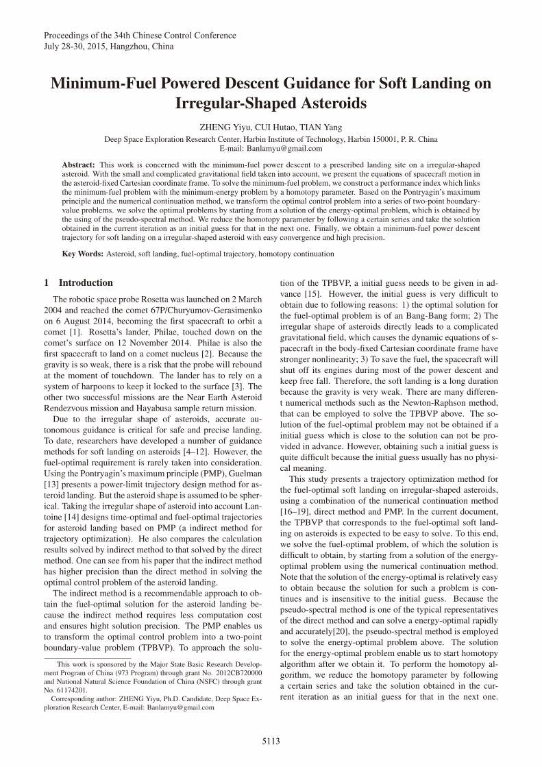
2.1 Dynamic EquationAs shown in Fig. 1, the asteroid-fixed Cartesian coordi-

nate frame (x, y, z) and inertial Cartesian coordinate frame

(X,Y, Z) share their origins at the center of mass, and have

the same z-axis, about which it’s assumed that the asteroid

rotation speed is a constant rotation rate ω. The asteroid-

fixed Cartesian coordinate frame aligns the x-, y-, and z-axes

along the axes of minimum, intermediate, and maximum in-

ertia respectively.

In the asteroid asteroid-fixed Cartesian coordinate frame,

Fig. 1: Inertial and asteroid-fixed Cartesian coordinate frame

relation [21].

the equations of the motion for the spacecraft can be written

as follows [4, 5, 11]:

x = 2ωy + ω2x+∂U

∂x+

Tmaxu

mcosβ cos θ (1)

y = −2ωx+ ω2y +∂U

∂y+

Tmaxu

mcosβ sin θ (2)

z =∂U

∂z+

Tmaxu

msinβ (3)

m = −Tmaxu

Ispge(4)

where r = [x, y, z]T

and v = [x, y, z]T

are the position

vector and velocity vector in the asteroid body-fixed Carte-

sian coordinate frame. Tmax is the maximum thrust magni-

tude, u ∈ [0, 1] is the thrust ratio. The angles β and θ serve

as the thrust direction. Isp is the thruster specific impulse,

ge is the Earth standard acceleration of gravity at sea level,

9.80665 m/s2. m is the instantaneous mass of the space-

craft. ∂U/∂x, ∂U/∂y and ∂U/∂z are the components of

the gradient of the gravitational potential U . The gravitation-

al potential is modeled as a second-order spherical harmonic

expansion given by [21]:

U =μ

r

{1 +

(rar

)2[1

2C20

(3z2

r2− 1

)+

+3C22x2 − y2

r2

]} (5)

where μ is the product of constant of universal gravitation

and the mass of target asteroid, ra is the referenced radius, ris the distance from the mass center of target asteroid to the

spacecraft.

The equations of the spacecraft motion can be written in a

compact form:

r = v (6)

v = f (r,v, ω) + ∂U/∂r + Tmaxuα/m (7)

m = −Tmaxu/Ispge (8)

where

f (r,v, ω) =

⎡⎣ 2ωy + ω2x

−2ωx+ ω2y0

⎤⎦

and the unit vector of thrust direction

α =

⎡⎣ cosβ cos θ

cosβ sin θsinβ

⎤⎦

2.2 Boundary ConditionsThe initial and final conditions are given by

r (t0) = r0,v (t0) = v0,m (t0) = mwet (9)

r (tf ) = rf ,v (tf ) = vf ,m (tf ) ≥ mdry (10)

where t0 and tf are the initial and final time, mwet is the

initial mass of the lander, mdry is the mass of the lander

without the propellant.

3 Minimum-Fuel Trajectory Design

The performance index Jm corresponds to the fuel-

optimal problem is

Jm =Tmax

Ispge

∫ tf

t0

udt (11)

and the performance index Je corresponds to the energy-

optimal problem is

Je =Tmax

Ispge

∫ tf

t0

u2dt (12)

To perform the homotopy algorithm, we construct a perfor-

mance index as follow

J =Tmax

Ispge

∫ tf

t0

(1− ζ)u+ ζu2dt (13)

where ζ is the homotopy parameter varying from 0 to 1.One

can see that if ζ = 1, then J = Je and if ζ = 0, then

J = Jm, which corresponds to the fuel-optimal problem.

To obtain the solution for the fuel-optimal problem, one can

solve a series of optimal control to minimize performance

index J by varying parameter ζ from 1 to 0.

5114

Based on the Pontryagin’s maximum principle (PMP),

we transform the optimal control problem into a two-point

boundary-value problem (TPBVP).

The Hamiltonian of the system is built as

H =λTr v + λT

v

(f (r,v, ω) +

∂U

∂r+

Tmaxu

mα

)

− λmTmaxu

Ispge

+Tmax

Ispge

[(1− ζ)u+ ζu2

] (14)

To minimize the Hamiltonian, the optimal thrust direction

and magnitude should be determined by

α∗ = −λv/ ‖λv‖ (15)

and

u∗ =

{u0, ζ = 0

uζ , else(16)

where

uζ =

⎧⎪⎨⎪⎩1, S < −ζ

0.5− 0.5S/ζ, |S| ≤ ζ

0, S > ζ

(17)

and

u0 =

⎧⎪⎨⎪⎩1, S < 0

u0 ∈ [0, 1] , S = 0

0, S > 0

(18)

with the switching function

S = 1− λm − Ispge ‖λv‖m

(19)

The costate differential equations are

λr = −∂H

∂r= −

(∂f (r,v, ω)

∂r+

∂2U

∂r2

)T

λv (20)

λv = −∂H

∂v= −λr −

(∂f (r,v, ω)

∂v

)T

λv (21)

λm = −∂H

∂m= −Tmax ‖λv‖

m2u (22)

with the final condition

λm (tf ) = 0 (23)

to be satisfied. Due to the free final time tf , the transversality

condition for Hamiltonian is

H (tf ) = 0 (24)

Once the initial costates [λr (t0) ,λv (t0) , λm (t0)]T

and

final time tf are specified, one obtains the final value r (tf ),v (tf ), λm (tf ) and H (tf ) by integrating the equations of

motion Eqs. (6)-(8) and the costate differential equations

Eqs. (20)-(22) from t = t0 to t = tf . The final value should

satisfy r (tf ) = rf , v (tf ) = vf , λm (tf ) = 0 and H (tf ) =0. Therefore, we obtain a TPBVP:{

x = φ (t,x, ζ, u∗) , t0 ≤ t ≤ tf

ρ (x (t0) ,x (tf )) = 0,(25)

where x = [r,v,m,λr,λv, λm]T

and

ρ (x (t0) ,x (tf )) =

⎡⎢⎢⎣

r (tf )− rfv (tf )− vf

λm (tf )H (tf )

⎤⎥⎥⎦

Considering that the TPBVP above can’t be solved direct-

ly due to the unknown final time tf , we define

τ = t/tf (26)

then one has{dxdτ = tfφ (τ,x, ζ, u∗) , 0 ≤ τ ≤ 1

ρ (x (0) ,x (1)) = 0,(27)

where x = [r,v,m,λr,λv, λm]T

and

ρ (x (0) ,x (1)) =

⎡⎢⎢⎣

r (1)− rfv (1)− vf

λm (1)H (1)

⎤⎥⎥⎦

For a given parameter ζ, the shooting function is

F (z, ζ) = [r (1)− rf ,v (1)− vf , λm (1) , H (1)]T= 0(28)

where z = [λr (τ0) ,λv (τ0) , λm (τ0) , tf ]T

is the combina-

tion of unknown initial costates and final time.

Varying parameter ζ from 1 to 0, we obtain a series of

nonlinear equations F (z, ζ) = 0. As mentioned above, the

homotopy parameter ζ links the mass criterion (ζ = 0) with

the energy criterion (ζ = 1). Let’s assume that the initial so-

lution z = z(1) for F(z, ζ(1) = 1

)= 0 which corresponds

to the energy-optimal problem has been obtained. Reduc-

ing the homotopy parameter ζ by following the certain se-

ries (ζ(1), ζ(2), ζ(3), ..., ζ(∗) = 0), and taking the solution

obtained in the current iteration as an initial guess for that

in the next one, the continuation method calculates further

solutions(z(1), ζ(1)

),(z(2), ζ(2)

),(z(3), ζ(3)

), ...,

until the target point (z(∗), ζ(∗)) which corresponds to the

fuel-optimal problem is reached. One can see that obtaining

the solution z(∗) only requires the solution for the energy-

optimal problem z(1). Compared to the fuel-optimal prob-

lem, the energy-optimal problem is relative easy to solve.

But it is also a challenge for us to find the solution because

the initial costates are guessed within an unbounded space.

Thus, to deal with this problem, we consider the adapting of

the direct method.

Due to ease of implementation, the direct method has been

widely adopted in engineering practice, especially in the

field of trajectory optimization. The pseudo-spectral method

is one of typical representatives of the direct method. It’s

recognized that the Karush-Kuhn-Tucker (KKT ) conditions

of Gauss pseudo-spectral method are equivalent with the one

order optimality conditions of the maximum principle [20].

This enables us to obtain an initial costates guess for the

energy-optimal problem F(z, ζ(1) = 1

)= 0 using pseudo-

spectral method to solve energy-optimal problem. Because

the solution for energy-optimal problem is a continuous con-

trol, the rapid convergence and high precision of pseudo-

spectral method can be achieved easily.

5115

4 Numerical Results

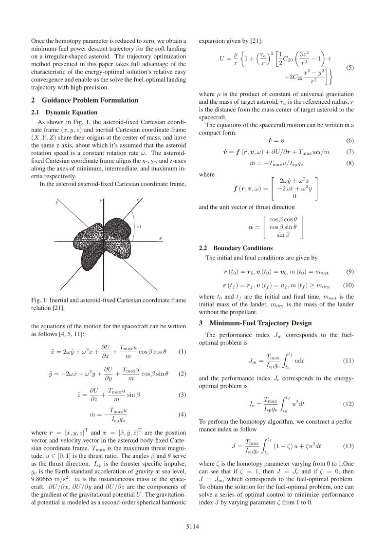
To illustrate the effectiveness of the proposed minimum-

fuel trajectory design method, in this section, a flight dynam-

ics scenario simulating a spacecraft landing on 433 Eros is

considered. The 3D model of 433 Eros is shown in Fig. 2.

The model parameters of the asteroid in the landing phase

are adopted from [5]. Other simulation conditions are spec-

ified by: Isp = 300 s, Tmax = 20 N, mwet = 550 kg,

r0 = [0.35, 0.30, 9.0]T

km, v0 = [−1.20, 0.20,−1.0]T

m/s,

rf = [0, 0, 7.0]T

km, vf = [0, 0, 0]T

m/s.

Fig. 2: 3D model of 433 Eros based on NEAR’s Laser

Rangefinder measurements [21].

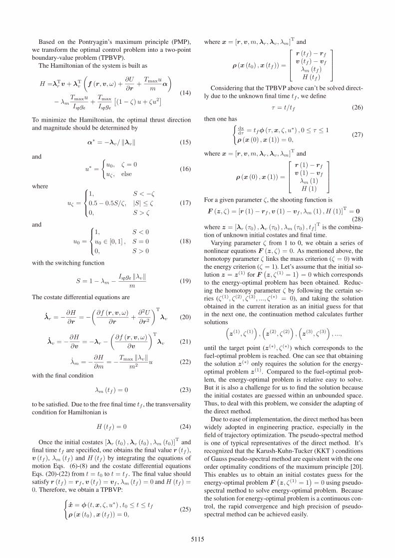
Calculation results of the pseudo-spectral method for

energy-optimal problem are shown in Fig. 3. It can be seen

that both the thrust ration and thrust direction angles are con-

tinuous. The initial costates and final time λr (τ0) , λv (τ0),λm (τ0), and tf for energy-optimal problem are shown in

Tab. 1. They are used as an initial guess for the homotopy

continuation method.

Calculation results of the homotopy continuation method

Table 1: Initial Costates and Final Time Guess Provided by

Pseudo-Spectral Method

Initial Guess Value

λr (τ0) [−1.0457, 6.3518, 0.3939]T

λv (τ0) [−0.7578, 2.5356,−0.5177]T

λm (τ0) 1.7407

tf 1412.29 s

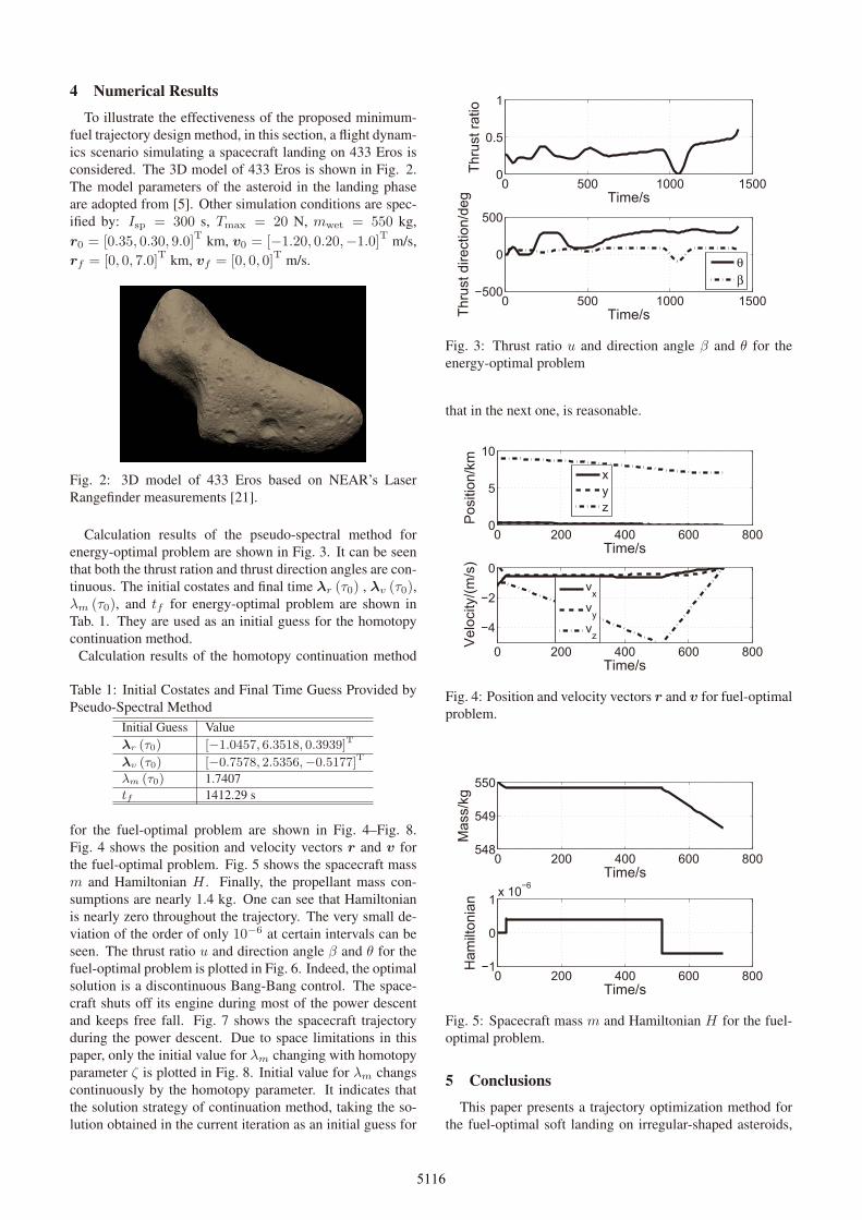
for the fuel-optimal problem are shown in Fig. 4–Fig. 8.

Fig. 4 shows the position and velocity vectors r and v for

the fuel-optimal problem. Fig. 5 shows the spacecraft mass

m and Hamiltonian H . Finally, the propellant mass con-

sumptions are nearly 1.4 kg. One can see that Hamiltonian

is nearly zero throughout the trajectory. The very small de-

viation of the order of only 10−6 at certain intervals can be

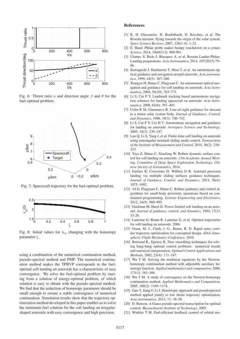
seen. The thrust ratio u and direction angle β and θ for the

fuel-optimal problem is plotted in Fig. 6. Indeed, the optimal

solution is a discontinuous Bang-Bang control. The space-

craft shuts off its engine during most of the power descent

and keeps free fall. Fig. 7 shows the spacecraft trajectory

during the power descent. Due to space limitations in this

paper, only the initial value for λm changing with homotopy

parameter ζ is plotted in Fig. 8. Initial value for λm changs

continuously by the homotopy parameter. It indicates that

the solution strategy of continuation method, taking the so-

lution obtained in the current iteration as an initial guess for

0 500 1000 15000

0.5

1

Time/s

Thru

st ra

tio

0 500 1000 1500500

0

500

Time/sThru

st d

irect

ion/

deg

θβ

Fig. 3: Thrust ratio u and direction angle β and θ for the

energy-optimal problem

that in the next one, is reasonable.

0 200 400 600 8000

5

10

Time/s

Pos

ition

/km

0 200 400 600 800

4

2

0

Time/s

Vel

ocity

/(m/s

)xyz

vx

vy

vz

Fig. 4: Position and velocity vectors r and v for fuel-optimal

problem.

0 200 400 600 800548

549

550

Time/s

Mas

s/kg

0 200 400 600 8001

0

1 x 10 6

Time/s

Ham

ilton

ian

Fig. 5: Spacecraft mass m and Hamiltonian H for the fuel-

optimal problem.

5 Conclusions

This paper presents a trajectory optimization method for

the fuel-optimal soft landing on irregular-shaped asteroids,

5116

0 200 400 600 8000

0.5

1

t/s

Thru

st ra

tio

0 200 400 600 8000

50

100

t/sThru

st d

irect

ion/

deg

θβ

Fig. 6: Thrust ratio u and direction angle β and θ for the

fuel-optimal problem.

0.2

0

0.2

0.4

0

0.2

0.46

7

8

9

x/kmy/km

z/km

SpacecraftTarget

Fig. 7: Spacecraft trajectory for the fuel-optimal problem.

0 0.2 0.4 0.6 0.8 11.5

2

2.5

ζ

λ m(0

)

Fig. 8: Initial values for λm changing with the homotopy

parameter ζ.

using a combination of the numerical continuation method,

pseudo-spectral method and PMP. The numerical continu-

ation method makes the TPBVP corresponds to the fuel-

optimal soft landing on asteroids has a characteristic of easy

convergence. We solve the fuel-optimal problem by start-

ing from a solution of energy-optimal problem, of which

solution is easy to obtain with the pseudo-spectral method.

We find that the reduction of homotopy parameter should be

small enough to ensure a stable convergence of numerical

continuation. Simulation results show that the trajectory op-

timization method developed in this paper enables us to solve

the minimum-fuel solution for the soft landing on irregular-

shaped asteroids with easy convergence and high precision.

References

[1] K. H. Glassmeier, H. Boehnhardt, D. Koschny, et al. The

Rosetta mission: flying towards the origin of the solar system.

Space Science Reviews, 2007, 128(1-4): 1–21.

[2] E. Hand. Philae probe makes bumpy touchdown on a comet.

Science, 2014, 346(6212): 900-901.

[3] Ulamec S, Biele J, Blazquez A, et al. Rosetta Lander-Philae:

Landing preparations. Acta Astronautica, 2014, 107(2015):79–

86.

[4] Kawaguchi J, Hashimoto T, Misu T, et al. An autonomous op-

tical guidance and navigation around asteroids. Acta astronau-tica, 1999, 44(5): 267–280.

[5] Xiangyu H, Hutao C, Pingyuan C. An autonomous optical nav-

igation and guidance for soft landing on asteroids. Acta Astro-nautica, 2004, 54(10): 763–771.

[6] Li S, Cui P Y. Landmark tracking based autonomous naviga-

tion schemes for landing spacecraft on asteroids. Acta Astro-nautica, 2008, 62(6): 391–403.

[7] Colin R M, Gianmarco R. Line-of-sight guidance for descent

to a minor solar system body. Journal of Guidance, Control,and Dynamics, 1996, 19(3): 740–742.

[8] Li S, Cui P Y, Cui H T. Autonomous navigation and guidance

for landing on asteroids. Aerospace Science and Technology,

2005, 10(3): 239–247.

[9] Lan Q, Li S, Yang J, et al. Finite-time soft landing on asteroids

using nonsingular terminal sliding mode control. Transactionsof the Institute of Measurement and Control, 2014, 36(2): 216–

223.

[10] Yiyu Z, Hutao C, Xiaofang W. Robust dynamic surface con-

trol for soft landing on asteroids. 11th Academic Annual Meet-ing, Committee of Deep Space Exploration Technology, Chi-nese Society of Astronautics, 2014.

[11] Furfaro R, Cersosimo D, Wibben D R. Asteroid precision

landing via multiple sliding surfaces guidance techniques.

Journal of Guidance, Control, and Dynamics, 2013, 36(4):

1075–1092.

[12] AI G, Pingyuan C, Hutao C. Robust guidance and control al-

gorithms for small-body proximity operations based on con-

strained programming. Systems Engineering and Electronics,

2012, 34(5): 989–995.

[13] Guelman M, Harel D. Power limited soft landing on an aster-

oid. Journal of guidance, control, and dynamics, 1994, 17(1):

15-20.

[14] Lantoine G, Braun R, Lantoine G, et al. Optimal trajectories

for soft landing on asteroids. 2006.

[15] Grant, M. J., Clark, I. G., Braun, R. D. Rapid entry corri-

dor trajectory optimization for conceptual design. AIAA Atmo-spheric Flight Mechanics Conference, 2010.

[16] Bertrand R., Epenoy R. New smoothing techniques for solv-

ing bang-bang optimal control problems: numerical results

and statistical interpretation. Optimal Control Applications andMethods, 2002, 23(4): 171–197.

[17] Wu T M. Solving the nonlinear equations by the Newton-

homotopy continuation method with adjustable auxiliary ho-

motopy function. Applied mathematics and computation, 2006,

173(1): 383–388.

[18] Wu T M. A study of convergence on the Newton-homotopy

continuation method. Applied Mathematics and Computation,

2005, 168(2): 1169–1174.

[19] Guo T, Jiang F, Li J. Homotopic approach and pseudospectral

method applied jointly to low thrust trajectory optimization.

Acta Astronautica, 2012, 71: 38–50.

[20] D. Benson. A Gauss pseudo-spectral transcription for optimal

control. Massachusetts Institute of Technology, 2005.

[21] Winkler T M. Fuel-efficient feedback control of orbital mo-

5117

tion around irregular-shaped asteroids. Iowa State University,

2013.

5118

View publication statsView publication stats