MINIMUM ENERGY BROADCAST IN DUTY CYCLED ... ENERGY BROADCAST IN DUTY CYCLED WIRELESS SENSOR NETWORKS...
124
MINIMUM ENERGY BROADCAST IN DUTY CYCLED WIRELESS SENSOR NETWORKS Mosarrat Jahan A thesis in The Department of Computer Science and Software Engineering Presented in Partial Fulfillment of the Requirements For the Degree of Master of Computer Science Concordia University Montr´ eal, Qu´ ebec, Canada April 2012 c Mosarrat Jahan, 2012
Transcript of MINIMUM ENERGY BROADCAST IN DUTY CYCLED ... ENERGY BROADCAST IN DUTY CYCLED WIRELESS SENSOR NETWORKS...
MINIMUM ENERGY BROADCAST IN DUTY CYCLED
WIRELESS SENSOR NETWORKS
Mosarrat Jahan
A thesis
in
The Department
of
Computer Science and Software Engineering
Presented in Partial Fulfillment of the Requirements
For the Degree of Master of Computer Science
Concordia University
Montreal, Quebec, Canada
April 2012
c© Mosarrat Jahan, 2012

Concordia University
School of Graduate Studies
This is to certify that the thesis prepared
By: Mosarrat Jahan
Entitled: Minimum Energy Broadcast in Duty Cycled Wireless Sensor Networks
and submitted in partial fulfillment of the requirements for the degree of
Master of Computer Science
complies with the regulations of this University and meets the accepted standards with
respect to originality and quality.
Signed by the final examining commitee:
Chair
Dr. R. Witte
Examiner
Dr. J. Opatrny
Examiner
Dr. T. Fevens
Supervisor
Dr. L. Narayanan
Approved by
Chair of Department or Graduate Program Director
20
Robin A.L. Drew, Ph.D.,ing., Dean
Faculty of Engineering and Computer Science

Abstract
Minimum Energy Broadcast in Duty Cycled Wireless Sensor Networks
Mosarrat Jahan
We study the problem of finding a minimum energy broadcast tree in duty cycled wireless
sensor networks. In such networks, every node has a wakeup schedule and is awake and
ready to receive packets or transmit in certain time slots during the schedule and asleep
during the rest of the schedule. We assume that a forwarding node needs to stay awake
to forward a packet to the next hop neighbor until the neighbor is awake. The minimum
energy broadcast tree minimizes the number of additional time units that nodes have to
stay awake in order to accomplish broadcast. We show that finding the minimum energy
broadcast tree is NP-hard. We give two algorithms for finding energy-efficient broadcast
trees in such networks. We performed extensive simulations to study the performance of
these algorithms and compare them with previously proposed algorithms. Our results show
that our algorithms exhibit the best performance in terms of average number of additional
time units a node needs to be awake, as well as in terms of the smallest number of highly
loaded nodes, while being competitive with previous algorithms in terms of the total number
of transmissions and delay.
iii
Acknowledgments
First and foremost I would like to express my gratefulness to Almighty Allah to make this
thesis possible.
I would like to express my sincere gratitude to my supervisor Dr. Lata Narayanan.
Her invaluable guidance and encouragement made my thesis work a wonderful learning
experience. It is a great opportunity for me to interact with her that enrich my growth
as a student as well as a researcher. Thanks to Dr. Lata for her insightful comments
and continuous support for the whole duration of my research work. Her endless valuable
suggestions and comments gradually matured my research work.
I wish to thank my colleagues and friends for their continuous encouragement. Special
thanks to my friend Shaily Kabir and Rajneesh Kumar and my elder sister Upama Kabir.
They always motivate me to keep faith in myself.
Finally I would like to express my deepest gratitude to my beloved parents, A. F. M
Shahjahan and Shireen Akter, for their unconditional love, continuous support and having
faith in me. Without their encouragement, it is not possible for me to finish the degree.
iv
Contents
List of Figures viii
List of Tables xi
1 Introduction 1
1.1 Broadcast Operation in Duty Cycled WSN . . . . . . . . . . . . . . . . . . 4
1.2 Summary of Contributions . . . . . . . . . . . . . . . . . . . . . . . . . . . . 6
1.3 Outline of Thesis . . . . . . . . . . . . . . . . . . . . . . . . . . . . . . . . . 7
2 Related Work 8
2.1 Broadcasting in WSN . . . . . . . . . . . . . . . . . . . . . . . . . . . . . . 8
2.1.1 Neighbor-Knowledge based Broadcasting . . . . . . . . . . . . . . . 9
2.1.2 Adaptive Broadcasting . . . . . . . . . . . . . . . . . . . . . . . . . . 10
2.1.3 Probability-Based Broadcasting . . . . . . . . . . . . . . . . . . . . . 12
2.1.4 Energy Efficient Broadcasting . . . . . . . . . . . . . . . . . . . . . . 13
2.1.5 Multipoint Relay based Broadcasting . . . . . . . . . . . . . . . . . . 17
2.1.6 Connected Dominating Set based Broadcasting . . . . . . . . . . . . 20
2.1.7 RNG and LMST based Broadcasting . . . . . . . . . . . . . . . . . . 21
2.2 Broadcasting in Duty Cycled WSN . . . . . . . . . . . . . . . . . . . . . . . 25
2.2.1 Centralized Algorithms . . . . . . . . . . . . . . . . . . . . . . . . . 25
2.2.2 Distributed Algorithms . . . . . . . . . . . . . . . . . . . . . . . . . 31
2.2.3 Differences with Our Work . . . . . . . . . . . . . . . . . . . . . . . 35
v
3 Algorithms and NP-Completeness 37
3.1 Definitions and Preliminaries . . . . . . . . . . . . . . . . . . . . . . . . . . 37
3.2 NP-Completeness of MEBT Problem . . . . . . . . . . . . . . . . . . . . . . 39
3.3 Algorithms . . . . . . . . . . . . . . . . . . . . . . . . . . . . . . . . . . . . 42
3.3.1 Spanning Tree with Incremental Cost (STIC) Algorithm . . . . . . . 43
3.3.2 MST Edmonds Algorithm . . . . . . . . . . . . . . . . . . . . . . . . 53
3.3.3 The Sweep Operation . . . . . . . . . . . . . . . . . . . . . . . . . . 56
4 Experimental Results 62
4.1 Performance Comparison of all Algorithms without Sweep Operation . . . . 63
4.1.1 Average Number of Additional Active Time Units per Node . . . . . 63
4.1.2 Energy Distribution . . . . . . . . . . . . . . . . . . . . . . . . . . . 66
4.1.3 Number of Node Transmissions . . . . . . . . . . . . . . . . . . . . . 69
4.1.4 Maximum Delay of Broadcast Operation . . . . . . . . . . . . . . . . 72
4.1.5 Average Delay of Broadcast Operation . . . . . . . . . . . . . . . . . 74
4.2 Performance Analysis of Various Versions of STIC Algorithm . . . . . . . . 77
4.2.1 Average Number of Additional Active Time Units per Node . . . . . 77
4.2.2 Energy Distribution . . . . . . . . . . . . . . . . . . . . . . . . . . . 78
4.2.3 Number of Node Transmissions . . . . . . . . . . . . . . . . . . . . . 78
4.2.4 Maximum Delay of Broadcast Operation . . . . . . . . . . . . . . . . 79
4.2.5 Average Delay of Broadcast Operation . . . . . . . . . . . . . . . . . 80
4.3 Performance Analysis of Various Versions of MST Edmonds Algorithm . . . 80
4.3.1 Average Number of Additional Active Time Units per Node . . . . . 81
4.3.2 Energy Distribution . . . . . . . . . . . . . . . . . . . . . . . . . . . 81
4.3.3 Number of Node Transmissions . . . . . . . . . . . . . . . . . . . . . 82
4.3.4 Maximum Delay of Broadcast Operation . . . . . . . . . . . . . . . . 82
4.3.5 Average Delay of Broadcast Operation . . . . . . . . . . . . . . . . . 84
4.4 Summary of Effect of Sweep Operation . . . . . . . . . . . . . . . . . . . . . 86
4.5 Performance Comparison of all Algorithms with Sweep Operations . . . . . 86
vi
4.5.1 Average Number of Additional Active Time Units per Node . . . . . 87
4.5.2 Distribution of Energy Usage . . . . . . . . . . . . . . . . . . . . . . 88
4.5.3 Number of Node Transmissions . . . . . . . . . . . . . . . . . . . . . 90
4.5.4 Maximum Delay of Broadcast Operation . . . . . . . . . . . . . . . . 91
4.5.5 Average Delay of Broadcast Operation . . . . . . . . . . . . . . . . . 92
4.6 Impact of Node Density . . . . . . . . . . . . . . . . . . . . . . . . . . . . . 96
4.7 Impact of Number of Nodes . . . . . . . . . . . . . . . . . . . . . . . . . . . 98
4.8 Impact of Schedule Length . . . . . . . . . . . . . . . . . . . . . . . . . . . 101
5 Conclusions and Future Work 104
Bibliography 105
vii

List of Figures
1 Abstract shapes of C(n) and A(n) . . . . . . . . . . . . . . . . . . . . . . . 12
2 The edge (u, v) not in E because of w . . . . . . . . . . . . . . . . . . . . . 22
3 Four cases of connecting a Covi(v) to the existing Tbcast through v . . . . . 26
4 G for variables x1, x2, x3 and C1 = x1∨x2
∨x3, C2 = x1
∨x2
∨x3 . . . . . 40
5 Broadcast Tree of G with W = 3 . . . . . . . . . . . . . . . . . . . . . . . . 41
6 Example of a duty cycled WSN G used to illustrate algorithms . . . . . . . 43
7 Construction of T with STIC algorithm with cost(T )=15 . . . . . . . . . . 47
8 Construction of T with STIC algorithm with cost(T )=15 . . . . . . . . . . 48
9 Construction of T with STIC algorithm with cost(T )=15 . . . . . . . . . . 49
10 Construction of T with STIC algorithm with cost(T )=15 . . . . . . . . . . 50
11 Construction of T with STIC algorithm with cost(T )=15 . . . . . . . . . . 51
12 Construction of T with STIC algorithm with cost(T )=15 . . . . . . . . . . 52
13 Construction of T with MST Edmonds algorithm with cost(T )=11 . . . . . 57
14 Construction of T with MST Edmonds algorithm with cost(T )=11 . . . . . 58
15 S as well as broadcast tree T obtained after extraction phase . . . . . . . . 59
16 Sweep Operation on T . . . . . . . . . . . . . . . . . . . . . . . . . . . . . . 61
17 Average no. of additional active time units per node at node density 8 for
all values of sch len and N = 400 . . . . . . . . . . . . . . . . . . . . . . . . 63
18 Average no. of additional active time units per node for all values of sch len
and N = 400 . . . . . . . . . . . . . . . . . . . . . . . . . . . . . . . . . . . 64
viii

19 Distribution of Energy Usage at node density = 12 whenN=400 and sch len =
15 . . . . . . . . . . . . . . . . . . . . . . . . . . . . . . . . . . . . . . . . . 66
20 Total number of node transmissions at node density 12 for sch len = 20 . . 70
21 Total number of node transmissions for sch len = 20 . . . . . . . . . . . . . 71
22 Maximum Delay of the Network at node density 12 for sch len = 20 . . . . 72
23 Maximum Delay of the Network at node density 10 and 8 for sch len = 20 . 73
24 Average Delay of the Broadcast Opeation at node density 12 for sch len = 20 75
25 Average Delay of the Network at node density 10 and 8 for sch len = 20 . . 76
26 Average no. of additional active time units per node for various versions of
STIC algorithm at node density = 12 and N=400 . . . . . . . . . . . . . . 77
27 Distribution of Energy Usage for STIC and STIC inc algorithms at node
density = 12 for N=400 and sch len=15 . . . . . . . . . . . . . . . . . . . . 78
28 Number of node transmissions for STIC and STIC inc at node density = 12
for sch len=20 . . . . . . . . . . . . . . . . . . . . . . . . . . . . . . . . . . 79
29 Maximum Delay of the Network for STIC and STIC bfs at node density 12
for sch len = 20 . . . . . . . . . . . . . . . . . . . . . . . . . . . . . . . . . . 80
30 Average Delay of the Network for STIC and STIC bfs at node density 12 for
sch len = 20 . . . . . . . . . . . . . . . . . . . . . . . . . . . . . . . . . . . 81
31 Average no. of additional active time units per node for various versions of
MST Edmonds algorithm at node density = 12 and N=400 . . . . . . . . . 82
32 Distribution of Energy Usage for MST Edmonds and MST Edmonds bfs al-
gorithms at node density = 12 for N=400 and sch len=15 . . . . . . . . . . 83
33 Number of node transmissions for MST Edmonds and MST Edmonds bfs at
node density = 12 for sch len=20 . . . . . . . . . . . . . . . . . . . . . . . . 83
34 Maximum Delay of the Network for MST Edmonds and MST Edmonds bfs
at node density 12 for sch len = 20 . . . . . . . . . . . . . . . . . . . . . . . 84
35 Average Delay of the Network for MST Edmonds and MST Edmonds bfs at
node density 12 for sch len = 20 . . . . . . . . . . . . . . . . . . . . . . . . 85
36 Maximum Delay of the Network at node density 12 for sch len = 20 . . . . 92
ix

37 Maximum Delay of the Network for sch len = 20 . . . . . . . . . . . . . . . 93
38 Average Delay of the Network at node density 12 for sch len = 20 . . . . . 94
39 Average Delay of the Network for sch len = 20 . . . . . . . . . . . . . . . . 95
40 Average no. of additional active time units per node for various values of N
at node density 12 when sch len=20 . . . . . . . . . . . . . . . . . . . . . . 97
41 Percentage of nodes with active time units 14 for various values of N at node
density 12 and sch len=15 . . . . . . . . . . . . . . . . . . . . . . . . . . . . 99
42 Average No. of Node Transmissions for various values of N at node density
12 and sch len=20 . . . . . . . . . . . . . . . . . . . . . . . . . . . . . . . . 100
43 Total Active Time Units per Node for STIC inc in a time period of 60 at
node density=12 . . . . . . . . . . . . . . . . . . . . . . . . . . . . . . . . . 102
44 Total Active Time Units per Node for MST Edmonds bfs in a time period
of 60 at node density=12 . . . . . . . . . . . . . . . . . . . . . . . . . . . . 103
x

List of Tables
1 Average Additional Active Time Units per Node with respect to MST Edmonds
for N=400 and sch len=20 . . . . . . . . . . . . . . . . . . . . . . . . . . . 65
2 Distribution of Energy Usage at node density 8 when N=400 and sch len=15 67
3 Distribution of Energy Usage at node density 10 when N=400 and sch len=15 68
4 Distribution of Energy Usage at node density 12 when N=400 and sch len=15 68
5 Percentage of Nodes with active time units 14 with respect to MST Edmonds
when N=400 and sch len=15 . . . . . . . . . . . . . . . . . . . . . . . . . . 69
6 Percentage of Nodes with active time units 7 with respect to MST Edmonds
when N=400 and sch len=15 . . . . . . . . . . . . . . . . . . . . . . . . . . 69
7 Total Number of Node Transmissions with respect to CSCA when N=400,
sch len=20 . . . . . . . . . . . . . . . . . . . . . . . . . . . . . . . . . . . . 70
8 Normalized Maximum Delay with respect to SDT whenN=400 and sch len=20 74
9 Normalized Average Delay with respect to SDT when N=400 and sch len=20 74
10 Improvements obtained by the sweep operation at node density 12 forN=400:
metric for best variant of sweep divided by metric for algorithm without sweep 86
11 Best version of sweep operation for various combinations of broadcast tree
algorithm and cost measure . . . . . . . . . . . . . . . . . . . . . . . . . . . 86
12 Average Additional Active Time Units per Node for N=400 and sch len = 20 87
13 Average Additional Active Time Units per Node with respect to MST Edmonds bfs
for N=400 and sch len = 20 . . . . . . . . . . . . . . . . . . . . . . . . . . 87
14 Percentage of Nodes with active time units 14 when N=400 and sch len=15 88
xi
15 Percentage of Nodes with active time units 7 when N=400 and sch len=15 88
16 Percentage of Nodes with active time units of 14 with respect to MST Edmonds bfs
when N=400 and sch len=15 . . . . . . . . . . . . . . . . . . . . . . . . . . 89
17 Percentage of Nodes with active time units of 7 with respect to MST Edmonds bfs
when N=400 and sch len=15 . . . . . . . . . . . . . . . . . . . . . . . . . . 89
18 Number of Node Transmissions when N=400 and sch len=20 . . . . . . . . 90
19 Number of Node Transmissions with respect to CSCA bfs when N=400 and
sch len=20 . . . . . . . . . . . . . . . . . . . . . . . . . . . . . . . . . . . . 90
20 Normalized Maximum Delay with respect to SDT whenN=400 and sch len=20 91
21 Normalized Average Delay with respect to SDT when N=400, sch len=20 . 94
xii
Chapter 1
Introduction
A Wireless Sensor Network (WSN) is a densely populated network consisting of a large
number of battery-operated sensor nodes. Sensor nodes are low power devices that usually
contain one or more sensors, a processor, memory, a power supply, a radio and an actuator.
Such a node utilizes a wide variety of sensors like mechanical, thermal, biological, chemical,
optical, magnetic etc. to measure different aspects of the environment [2]. Sensor nodes are
equipped with a processor and a limited size memory and thus capable of performing simple
calculations. Wireless communication among the nodes is established through the radio. If
two nodes are within the transmission range of each other they can communicate directly.
Otherwise intermediate nodes between the two end points should forward the packets. The
positions of the sensor nodes in a WSN are not usually predetermined and they are deployed
in large number to achieve accurate computation and to overcome the limitations imposed
by short transmission range of nodes. In most applications of WSNs, a large body of sensor
nodes are deployed in an ad hoc manner to monitor certain aspects of the environment and
the nodes periodically send data to a base station.
WSNs have huge potential in a wide range of applications such as health, military,
home and environment. Due to the rapid deployment, self-organization, and fault tolerance
properties, WSNs are very promising in military applications. They can be exploited for
military command, control, communication, computing, intelligence, surveillance, recon-
naissance and targeting systems [3]. Particularly, in a battlefield a WSN can be utilized
1
for surveillance of critical terrains and routes. In a target tracking system, a WSN can be
used for detection and identification of intruders. Moreover, a WSN can be exploited for
gathering information about battle damage assessment. In the health care setting, sensor
nodes can be deployed to monitor the conditions of patients and assist disabled patients.
The chance of getting and prescribing the wrong medication to the patients is decreased if
sensor nodes are used to administer medications. For home applications, sensor nodes and
actuators can be included in appliances like vacuum cleaners, microwave ovens, refrigerators
etc. Sensor nodes inside these domestic devices can interact with each other using external
networks or the Internet. They allow the end users to control home devices more conve-
niently either locally or remotely. In environmental applications, WSNs can be exploited for
tracking the movements of animals and monitoring environmental conditions affecting crops
and livestock. They can be utilized for large-scale earth monitoring, planetary exploration,
biological, earth, and environmental monitoring in marine, soil and atmospheric contexts,
forest fire detection, pollution studies etc. Some of the commercial applications include
managing inventory, monitoring product quality, monitoring material fatigue, environment
control in office building and monitoring disaster areas.
Due to the huge prospects for WSNs, significant research has been conducted to devise
suitable solutions for various challenges of WSN as well as to adapt the existing proto-
cols of other networks for WSN. Unlike traditional networks, a WSN has its own design
issues and resource limitations. Resource constraints include limited energy source, short
communication range, low bandwidth and limited processing and storage capacity in each
node. Generally in WSNs a large number of sensor nodes work together unattended. Sen-
sor nodes may be deployed in hostile environments such as disaster recovery where it is not
possible to replace the battery of the nodes. Thus, the topology of a WSN changes because
of the death of nodes due to running out of power as well as because of the addition of
new nodes. This in turn indicates that the protocols and algorithms for WSNs should be
designed with self-organizing capability. Moreover, the failure of nodes should not affect
the overall operation of a WSN; this property is known as fault tolerance. Due to large
scale deployment, protocols and algorithms for WSN should be scalable, and resilient to
2

changes in topology. Moreover wise utilization of battery power is essential for long time
operation of WSN. Malfunctioning of sensor nodes significantly changes the topology and
thus necessitates rerouting of data packets and reorganization of the network. Thus, power
conservation and power management take on additional importance. A huge amount of
research is going on to design power-aware protocols and algorithms for WSNs. Routing in
WSNs is more challenging due to their unique characteristics that distinguish them from
other wireless networks [4]. Due to large scale deployment of sensor nodes it is not possible
to build a global addressing scheme as the overhead of ID maintenance is high. Moreover,
sensor nodes deployed in an ad hoc fashion should be self-organizing in order to get itself
accustomed in the existing WSN. Routing in WSN is data-centric as there is no global
addressing scheme. Due to tight constraints on energy, processing, and storage capacities,
routing in WSN requires careful resource management.
Due to extremely limited energy it is not feasible for WSN to operate as networks that
are always operational. The fundamental idea of duty cycled WSNs is to reduce the time
spent by a node in idle state or overhearing other transmissions by putting the node in sleep
state. Each sensor keeps itself active for only a very brief period of time and this is known
as active state, while it stays dormant for a long time. During its active state a node can
sense an event, transmit a packet or receive a packet, or even stay idle. During the sleep
state, a node turns all its functional units off except a timer, to wake itself up after a fixed
amount of time. The concept of a duty cycle is represented by a periodic wake up schedule
associated with every sensor node. The duty cycle is measured as the ratio of the number
of active time units to the total number of time units. It indicates how long a node spends
in active state. A small duty cycle signifies that a node is asleep most of the time. The
duty cycle of a WSN is determined based on the requirements of the applications for which
the network is deployed.
Routing in duty cycled WSN becomes more complicated since a transmitting node may
not be active at the same time unit as its neighbors. Thus a node needs to wait until it can
forward a message to its neighbors. Unlike other wireless networks where a node can reach
all its neighbors with one message, in a duty cycled network, a node may need to transmit
3
to all its neighbors separately. Providing an energy efficient communication mechanism for
duty cycled WSN is the main focus of this thesis.
1.1 Broadcast Operation in Duty Cycled WSN
Broadcasting is a fundamental operation in wireless networks where data transmitted by
a node is sent to all nodes in the networks. For example, various reactive or on-demand
routing protocols such as AODV, DSR etc utilize the concept of discovering of a route
when the actual need to route data arises [14]. The route discovery mechanism depends
on the broadcast operation to determine a route between a source and destination nodes.
Mobile Ad-hoc Network (MANET) can use delay-efficient broadcast operation to quickly
disseminate information such as an link breakage message to the whole network so that the
topology information is updated in every node [47]. Many real-time applications such as
audio conferencing also require a low-latency broadcast operation to deliver delay-sensitive
data over the wireless ad hoc networks.
In WSNs as well as in duty cycled WSNs, broadcast operation has significant impact.
In most applications of WSN, a large number of sensor nodes monitor the occurrence of an
event and inform a central node known as the sink. Conversely, the sink node broadcasts
control messages during network configuration time and interest/ query messages at the
time of data acquisition. Broadcast operation is one of the basic communication services in
WSN that is used to establish communication between sink node and other sensor nodes.
Non-sink sensor nodes may also broadcast messages in order to synchronize with other
nodes to monitor certain events [46]. Various routing protocols for WSN also use broadcast
operation as the integral part of their operation. For example, in LEACH (Low-Energy
Adaptive Clustering Hierarchy) [15], a node selects itself as a cluster head and informs all
the nodes in the network through broadcasting an advertisement message. Various data
centric routing protocols also utilize broadcast operation for the purpose of data collection.
For example, in directed diffusion [21], the sink node requests data by broadcasting interest
messages. In SPIN (Sensor Protocols for Information via Negotiation) [16], when a node
4
has new data to share, it broadcasts an advertisement message to all nodes in the network
about the new data.
Multicasting is an important mechanism of communication used for sending information
to a group of nodes. Many researchers utilize the mechanism of broadcast operation to
determine a suitable solution for multicasting. They first construct a broadcast tree that
will cover all the nodes in the networks and then eliminate the transmissions that are not
directed to the members of the multicast group. This application of broadcast tree is used
in [49], [51].
In the literature most research has been aimed on minimizing the number of transmis-
sions in a broadcast operation while achieving whole network coverage as well as providing
reliable broadcast operation by minimizing collisions. Moreover some work has been moti-
vated by the need to minimize the delay of the broadcast operation.
Designing energy-efficient broadcast algorithm for duty cycled WSNs is a challenging
problem as sensor nodes switch between active and sleep modes. Clearly the energy con-
sumption during sleep mode is much less than that in any other mode. However, going
into sleep mode is not without cost. In fact, there is a significant amount of energy as
well as time required to change from sleep mode back to transmit mode. To get an idea of
switching cost we consider an example mentioned in [24]. When a node wakes up it listens
the channel for a brief period of time and measures the signal strength. If it is greater than
a threshold value, the node remains active to receive transmission. Otherwise, it will go
to sleep. The procedure is known as sniffing the channel [24]. For Chipcon CC1100 radio,
if a node wakes up once every second the average current consumption over 1 second is
15μA that will cause a charge draw of 15μC. Whereas, the average current draw is 15mA
for receiving or transmitting a packet. Thus, in a day of operation of the network, the total
energy consumption of a node due to wakeup is equal to 15μA*3V *86400s = 3.9J that
can be utilized to transmit or receive almost 21 Mbits of data. Recently several papers
have pointed out that neglecting the so-called switching energy to switch from one mode
to another can lead to algorithms with sub-optimal energy consumption or reduce network
lifetime [5,9,23,24]. Ruzzelli et al. [38] report measurements on three different chipsets for
5

sensor nodes that show that at low traffic load, the switching energy can dominate the en-
ergy required for transmission. Thus, depending on the traffic conditions, it is not beneficial
to switch to sleep mode at every opportunity.
When a node has a packet to transmit it has two options. As the active time slots of its
neighbors are not necessarily synchronized either with the node itself or with each other,
one option is for the node to go into sleep mode and wake up and transmit the packet when
its first neighbor wakes up, and thereafter repeatedly switch between sleep and transmit
modes until it has delivered the packet to all the relevant neighbors. Indeed several papers
make this assumption in analyzing the energy costs of their algorithms [18, 46]. However,
as mentioned earlier, this model ignores the high switching cost of switching from sleep to
transmit mode. Another option as assumed in [43], is for the node to stay awake until it has
delivered the packet to next-hop neighbors. This option not only has the merit of simplicity,
it is clearly more energy-efficient when the switching cost is high, when there are many
neighbors, or not many slots in between the active times of different neighbors. This is the
model we assume in this thesis.
In this thesis, we address the energy inefficiency issue of the broadcast operation in duty
cycled WSNs and propose algorithms to minimize the total number of additional active
time units the nodes of a network need to be active during the broadcast operation. Given
the number of nodes N in a duty cycled WSN and a wakeup schedule of fixed length k for
every node, these algorithms construct a broadcast tree that will minimize the total number
of additional active time units nodes need to be awake. This problem is known as the
Minimum Energy Broadcast Tree (MEBT) problem.
1.2 Summary of Contributions
In this thesis we address the MEBT problem for duty cycled WSNs. In this section, we give
a summary of our results.
1. We show that the MEBT problem is NP-hard.
6

2. We propose two polynomial time algorithms to construct an energy-efficient broad-
cast tree for MEBT problem: Spanning Tree with Incremental Cost (STIC) and
MST Edmonds.
3. We describe several variants of a sweep operation similar to the one in [51], that can
be applied to a given broadcast tree to reduce its cost. Our experimental results show
that this operation substantially reduces the cost of the broadcast tree, and generally
also improves the performance according to other cost measures.
4. We evaluate the performance of the algorithms using extensive simulations and com-
pare the results with two existing algorithms named Centralized Set Cover based Ap-
proximation Algorithm (CSCA) [18] and Shortest Delay Tree(SDT) which is adapted
from One-to-All Broadcast Algorithm (OTAB) [22]. The experiments show that both
MST Edmonds and STIC have the best performance for the MEBT problem, and they
also result in fewer heavily loaded nodes as compared to the two existing algorithms.
Their performance is also competitive in terms of the number of node transmissions
and maximum and average delay.
1.3 Outline of Thesis
In Chapter 2, we present a literature review on broadcast problem in WSNs as well as in
duty cycled WSNs. In Chapter 3, we propose our algorithms for energy efficient broadcast
tree construction and illustrate the operation of the algorithms with a suitable example.
We analyze the performance of the proposed algorithms in Chapter 4. Some concluding
remarks and possible directions for future work are given in Chapter 5.
7
Chapter 2
Related Work
In this chapter we review the broadcast algorithms for wireless networks that exist in the
literature. We will discuss several important broadcast algorithms and try to give an idea
of the various trends of the research in this field. We first highlight various algorithms
for broadcasting in wireless sensor networks followed by a discussion about the broadcast
protocols in duty cycled wireless sensor networks.
2.1 Broadcasting in WSN
Broadcasting is an important communication paradigm in all networks including wireless
sensor networks. The simplest way to broadcast a packet is flooding. In this technique,
every node retransmits a packet once when it receives the packet for the first time. It is a
very simple technique and ensures that every node receives the packet. The disadvantage of
flooding is that it generates abundant retransmissions causing the wastage of battery energy
and bandwidth. Retransmissions by geographically close nodes result in message collisions
and channel contentions. This scenario is known as the broadcast storm problem [32].
Extensive research has been conducted to reduce the number of retransmissions during
the broadcast operation. This optimization leads to the design of energy efficient broadcast
protocols that are a necessity for energy-constrained wireless networks. Research is also
conducted to build up protocols that will achieve reachability as well as latency-optimized
8
operation.
To organize the discussion of protocols, we divide them into a number of groups depend-
ing on a number of aspects. Algorithms belonging to the same group have some common
characteristics. In the following subsections we will describe the algorithms from various
categories.
2.1.1 Neighbor-Knowledge based Broadcasting
Algorithms in this category are mainly inspired by the work of H. Lim and C. Kim [29]. They
proposed two flooding heuristics named Self-Pruning (SP) and Dominant-Pruning (DP). SP
utilizes the direct neighbor information. Node v piggybacks N(v) in the broadcast packet.
Another node u receiving the packet, checks whether N(u) −N(v) − {v} is empty. If it is
empty, u does not forward the packets as all its adjacent nodes already received the packet.
The time complexity of the SP is O(Δ), where Δ is the maximum degree of the tree.
A similar algorithm to SP is proposed by Peng et el. [34]. They utilize the local topology
information and the statistical information about duplicate messages to eliminate unnec-
essary transmissions. Every node has the knowledge of its 2-hop neighborhood. When a
node u receives a message m from a node v it records N(v) ∩ {v} in its broadcast cover
set C(u,m). Then it checks whether N(u) ⊆ N(v) ∩ {v} and if it is true, then node u
avoids transmission of m. Otherwise, if message m is received for the first time, u initializes
C(u,m) to N(v)∩{v} and waits for a random delay period. During this time node u records
N(v) ∩ {v} in C(u,m) for any v from which it receives a duplicate of m. When the delay
period is expired, if N(u) ⊆ C(u,m), then u avoids the rebroadcast of m. Otherwise u will
rebroadcast the message m. The delay period is selected carefully so that a node with more
neighbors broadcasts earlier as compared to other nodes.
DP uses the 2-hop neighborhood information. The sending node selects from its adjacent
nodes a set of forwarding nodes to relay the broadcast packet and appends the IDs of
the selected nodes in the broadcast packet which is known as the forward list. A node
in the forward list in turn selects the forwarding nodes from its 1-hop neighbors. This
process is continued until the broadcast operation is completed. On receiving a packet
9
from node u with v in the forward list, node v determines its forward list so that all
nodes within 2-hop distance from v receive the packet. Node v tries to cover all nodes in
U = N(N(v)) −N(u) −N(v), where N(u) and N(v) are the 1-hop neighbor list of u and
v, respectively. As nodes in N(u) have already received the packet and those in N(v) will
receive the packet when v will forward the packet, this algorithm selects a set of forwarding
nodes F = {f1, f2, ...., fm} from B(u, v) = N(v) −N(u) such that⋃
fi∈F (N(fi)⋂U) = U .
This algorithm repeatedly selects vk ∈ B(u, v) which can cover the maximum number of
uncovered neighbor nodes. Both SP and DP outperform blind flooding by reducing the
redundant retransmissions, while DP achieves the best result. DP obtains this result at the
cost of larger overhead of passing the forward list in the broadcast packet. This overhead
increases as the host mobility increases.
The authors of [30] identified the deficiencies of DP and proposed two algorithms that
reduce the forwarding set further by more effectively utilizing the 2-hop neighborhood in-
formation. In Total Dominant Pruning (TDP), N(N(u)) is piggybacked in the broadcast
packet from u. When another node v receives the packet, the 2-hop neighbor set that needs
to be covered by the forward list F of v is reduced to U = N(N(v)) − N(N(u)). As the
size of U is reduced, the size of F also gets reduced. The TDP algorithm consumes more
bandwidth as the 2-hop neighborhood information of each sender is piggybacked in the
broadcast packet. Partial Dominant Pruning (PDP) does not piggyback any neighborhood
information with the broadcast packet as in TDP but reduces nodes from U by excluding
P = N(N(u)⋂N(v)). Thus U will become N(N(v)) −N(u) −N(v) − P . The extra cost
of the PDP algorithm is that each forward node v needs to calculate P .
Simulation results show that both TDP and PDP significantly reduce the number of
forwarding nodes as compared to DP. TDP produces slightly better result than PDP and
PDP is cost effective since there is no piggybacking as in TDP and DP.
2.1.2 Adaptive Broadcasting
To alleviate the broadcast storm problem of simple flooding, several threshold-based broad-
casting techniques are proposed. The author of [32] proposed a counter-based scheme as
10
well as a location-based scheme for broadcast. In the counter-based scheme [32], every
host maintains a counter c for each packet. This counter c is used to keep a record of
the number of times a host has received a broadcast packet. When c reaches a predefined
threshold value C, the host refrains from rebroadcasting the packet as the additional cov-
erage achieved through this transmission is very low. In the location-based scheme [32],
each host is assumed to be equipped with a positioning device such as GPS. A receiver
can accurately calculate the additional coverage that can be achieved from the location of
the source from which it heard the broadcast packet. The receiving host uses a predefined
threshold A to determine whether it should rebroadcast or not. The location based scheme
achieved better performance in terms of both reachability and the amount of savings as
compared to the counter-based scheme as more accurate information is used.
The authors of [44] proposed improvements to both the counter-based and the location-
based schemes. Adaptive Counter-Based scheme [44], dynamically adjusts the threshold
value C(n) based on local neighbor information and introduces a time delay before broad-
casting a packet to reduce the number of redundant transmissions further. A small value of
C(n) can significantly reduce the number of redundancies in a dense network while achiev-
ing a better reachability. For sparse networks, greater values of C(n) should be used to
achieve reachability, which will increase the number of rebroadcasts. Based on the above
observations, the authors proposed abstract shapes of C(n) (shown in Figure 1). The
adaptive location-based scheme [44], dynamically adjusts the threshold value A(n) based
on neighbor information. The authors presented an abstract shape of threshold function
A(n) following the same observations for counter-based scheme. As shown in Figure 1,
when n < n1, A(n) should be 0 to enforce a host to rebroadcast. Between n1 and n2, A(n)
gradually increases to balance savings and reachability. After n > n2, A(n) = 0.187 is used
which is the expected additional coverage achieved after a host receives same broadcast
packet twice.
11
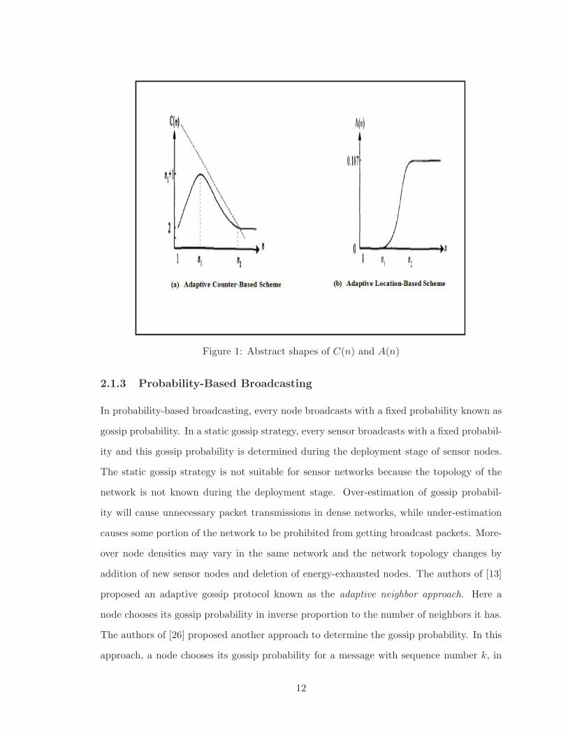
Figure 1: Abstract shapes of C(n) and A(n)
2.1.3 Probability-Based Broadcasting
In probability-based broadcasting, every node broadcasts with a fixed probability known as
gossip probability. In a static gossip strategy, every sensor broadcasts with a fixed probabil-
ity and this gossip probability is determined during the deployment stage of sensor nodes.
The static gossip strategy is not suitable for sensor networks because the topology of the
network is not known during the deployment stage. Over-estimation of gossip probabil-
ity will cause unnecessary packet transmissions in dense networks, while under-estimation
causes some portion of the network to be prohibited from getting broadcast packets. More-
over node densities may vary in the same network and the network topology changes by
addition of new sensor nodes and deletion of energy-exhausted nodes. The authors of [13]
proposed an adaptive gossip protocol known as the adaptive neighbor approach. Here a
node chooses its gossip probability in inverse proportion to the number of neighbors it has.
The authors of [26] proposed another approach to determine the gossip probability. In this
approach, a node chooses its gossip probability for a message with sequence number k, in
12
inverse proportion to the number of duplicate messages that were overheard for message
k − 1.
Kyasanur et al. [25] identified the deficiencies of the existing adaptive approaches and
proposed the smart gossip protocol for wireless sensor networks. In Smart Gossip, the
importance of each node v is quantified according to the number of nodes depend on v to
receive a disseminated message. When a large number of nodes depends on v, it will transmit
with higher probability while other less crucial nodes transmit with lower probability. This
protocol is completely decentralized and capable of handling wireless link failures and node
failures. This protocol significantly reduces energy expenditure by reducing the number of
forwarding nodes while achieving the reliability requirements of the application.
2.1.4 Energy Efficient Broadcasting
Every node v in a wireless network is associated with a power level Pv such that 1 ≤ Pv ≤m,Pv ∈ Z. Node v can select its own power level to reach its neighbors. Algorithms in this
category try to construct broadcast trees in order to minimize the total power expenditure to
accomplish the broadcast operation. W. Liang proved in [28] that the problem of assigning
power levels to minimize the total power expenditure is NP-Complete.
Wieselthier et al. [49] proposed three heuristic algorithms for constructing broadcast
trees. Broadcast Incremental Power (BIP) algorithm takes advantage of broadcast nature
of the wireless channel. This algorithm assumes that the locations of the nodes are fixed.
The power needed to maintain the link between node i and j is denoted by Pi,j = ri,j , where
ri,j is the distance between node i and j. If a node i is transmitting to its neighbors j and
k with transmission power Pi,j and Pi,k respectively, then a single transmission at power
Pi,{j,k} = max {Pi,j , Pi.k} is sufficient to reach both node j and k. This property is known
as wireless multicast advantage (WMA). BIP starts with a source s and adds a node that
can be reached from s with minimum power. For all nodes i ∈ T and for all adjacent nodes
j of i /∈ T , BIP evaluates the following equation:
Pi,j′ = Pi,j - P (i)
13
where,
Pi,j = Cost of transmission between node i and j.
P (i) = Power level at which i is already transmitting. If i is a leaf node, then P (i) = 0.
Pi,j′ = Incremental cost of i to associate j with i.
At every step, BIP selects a j with minimum Pi,j′ to be added to T and adjusts the cost
Pi,k′ of edges between i and k, where k is a neighbor of i not in T . This process continues
until all nodes are included in T . BIP is similar to Prim’s algorithm with only difference is
that BIP will dynamically update the cost at each step.
In Broadcast least-Unicast-Cost (BLU) algorithm [49], minimum cost paths from s to
every other node are determined and a broadcast tree is obtained by superimposing these
unicast paths. As BLU cannot take the advantage of WMA, it produces trees with higher
overall power expenditure.
The Broadcast Link-based MST(BLIMST) algorithm [49] associates link cost Pi,j with
each pair of nodes i and j. A minimum cost spanning tree is formed using standard MST
techniques. This algorithm also does not take the advantage of WMA.
Wieselthier et al. [49] also found that by rearranging the structure of the broadcast
tree significant reduction in overall power expenditure can be achieved. They proposed a
operation known as sweep. Given a broadcast tree, the sweep operation makes node v a
child of u instead of its previous parent w, if doing so reduces the power expenditure at w
without increasing the power expenditure at u.
The authors of [33] proposed an algorithm to maximize the network lifetime followed by
a broadcast operation. Given a sequence of broadcast operations, they tried to increase the
number of successful communications before the first communication fails. For this purpose,
they proposed an O(m logm) algorithm to construct a broadcast tree that maximizes the
critical energy of the network following a broadcast operation, where m denotes the number
of links in the network. The critical energy of a broadcast tree T is the minimum of the
remaining battery power of all the nodes in T followed by a broadcast operation. In T ,
the residual energy of node i is re(i, T ) = ce(i) − max{w(i, j)|j is a child of i in T},where ce(i) is the current energy of i before sending a message and w(i, j) is the energy
14
expended for transmitting a message from i to j. The critical energy CE(T ) following a
broadcast operation is CE(T ) = min{re(i, T )|1 ≤ i ≤ n}. The Maximum Critical Energy
Problem (MCEP), finds a broadcast tree T rooted at s such that CE(T ) is maximum. This
maximum value of CE(T ) is called the maximum critical energy and is denoted MCE(G,
s). This algorithm first constructs a sorted list L of all possible residual energy values. For
each node i of G, the set a(i) of residual energy values is defined as a(i) = {ce(i)− w(i, j)|(i, j) is an edge of G and ce(i) ≥ w(i, j)}. Set l(i) denotes the set of all possible values for
residual energy of i following a broadcast operation.
l(i) =
⎧⎪⎨⎪⎩
a(i) if i = s
a(i)⋃{c(i)} otherwise
Thus, L = sort(⋃
1≤i≤n l(i)). The algorithm performs binary search on L to determine
MCE(G,s). For each value q ∈ L, it determines whether there exists a broadcast tree rooted
at s such that CE(T ) > q, by performing breadth first or depth first search that avoids
edges (i, j) for which ce(i)− w(i, j) < q.
Chen et al. [8] proposed Power Adaptive Broadcasting (PAB) to adjust the transmission
power of a node based on its neighbor information. This information is obtained by ex-
changing the HELLO messages. Each HELLO message contains a list of 1-hop neighbors of
a node with the transmission power needed to reach them. In PAB, every node u starts with
the most distant node v that causes u to transmit at maximum power level Pmax = Pu,v.
Node u determines the subset of its 1-hop neighbors that can reach v and selects a neighbor
w that can reach v with minimum transmission power Pw,v. Node u calculates Pu,w + Pw,v
and if Pu,w+Pw,v < Pu,v it reduces its power level to a lower value and allows w to reach v.
This is known as local optimization. If u cannot find such a node it transmits using power
Pu,v. After reducing the transmission power level node u starts with the next furthest node
and tries to reduce its transmission radius by allowing other neighbor to reach the distant
node. This process stops when u cannot find such a neighbor. It may happen that when
a node receives a broadcast packet and calculates the local optimization it may considers
neighbor that already received the packet. To minimize this problem, after receiving a
15
packet, a node may wait for a randomly selected time period. During this time, if it finds
that some of its neighbors broadcast the same packet it eliminates these neighbors as well
as the nodes that receive the packet from the consideration of local optimization.
PAB will consume at most the energy consumed in a non-power- adaptive scheme in
which the nodes transmit at maximum power level and it achieves the same coverage as non-
adaptive schemes. Experimental results show that PAB reduces total energy consumption
about 40% as compared to the protocols that do not adapt the power level.
Weishelthier et el. [50] proposed two distributed versions of the centralized BIP algorithm
named as Distributed-BIP-All (Dist-BIP-A) and Distributed-BIP-Gateways (Dist-BIP-G).
In Dist-BIP-A, every node u knows the cost of the links between node u and its 1-hop
neighbors and also cost of the links between every pair of node u’s 1-hop neighbors. When
node u has a broadcast packet, it constructs a local BIP tree using this information and
broadcasts this tree to all its neighbors. When a node v becomes aware that it is in the tree
from some node u, it generates its local BIP tree and broadcasts to the neighbors. A node
v can hear from multiple parents but it becomes child of a node from which it hears for the
first time. Dist-BIP-All generates huge burden on MAC layer as every node performs the
broadcast operation. In Dist-BIP-G, every node u knows the cost of the links between u’
neighbors and their neighbors. Node u has no knowledge of the cost of the links between
its 2-hop neighbors v and w. Node u constructs local BIP tree using this information and
determines the gateway nodes from its 1-hop neighbors that cover one or more nodes in
its 2-hop. The set of gateway nodes of u covers all the 2-hop neighbors of u. After the
construction of BIP tree, node u broadcasts this information to all its neighbors. The links
between the gateways and their neighbors are not included in the global tree. Now only
the gateway nodes of u will construct their local BIP tree and broadcast this information.
It reduces the overhead on MAC layer as only fewer node will broadcast the BIP tree.
A localized version of BIP algorithm (LBIP) is proposed in [19]. In this method, each
node constructs a BIP tree within its 2-hop neighborhood using information provided by the
node from which it gets the broadcast message. Thus the tree is incrementally constructed.
The source node determines the BIP tree within its 2-hop neighborhood and selects the
16
nodes within its range that should relay the packet with which transmission radius. These
choices are forwarded with the broadcast packet. No instructions are given in the packets
for nodes that are designated as leaf nodes. When a node u receives the packet for the first
time from a node v, two cases can occur:
1. The packet contains some instructions for u. It starts constructing a BIP tree within
its own 2-hop neighborhood. But instead of starting with an empty tree, it uses the
information contained in the packet, that is with the neighbors assigned to it by v
and with its transmission range also fixed by v. In this way, nodes located exactly at
2 hops from u and 3 hops from v will be added to the tree.
2. There is no instruction for u. In this case, u will not rebroadcast the packet.
As the algorithm is localized one, it is possible that two different nodes may make conflicting
decisions that will lead to some nodes being uncovered. To avoid this situation, when a
node receives a broadcast packet, it will monitor its neighborhood for a fixed amount of
time. If the node finds that some of its neighbors do not get the packet, it can transmit the
packet to them whether it is instructed to do so or not. This ensures coverage at the cost
of some unnecessary transmissions. To minimize these unnecessary transmissions, the set
of monitored neighbors can be reduced to a smaller subset of neighbors using a subgraph
of the general graph such as RNG or LMST [19]. LBIP eliminates the overhead of message
exchange in distributed BIP and does not increase the size of the message significantly.
Experimental results showed that this algorithm has good performance at low density and
it is very energy efficient for higher densities with performance equal to BIP.
2.1.5 Multipoint Relay based Broadcasting
The authors of [36] proposed the mechanism to calculate multipoint relay (MPR) set. This
technique reduces the number of redundant message transmissions in broadcast operation.
The authors proved that the computation of MPR set with minimum size is NP-Complete
and proposed a heuristic technique to compute the MPR set. Each node calculates it
own MPR set independently and modifies its MPR set according to the changes in local
17

topology. Every node u starts with an empty MPR(u) set and selects those nodes v from
N(u) that are only neighbors of some 2-hop neighbors of u. Node u is called the MPR
selector of v. If there are some 2-hop neighbors that are not covered by MPR(u), a node
from N(u) that covers the largest number of 2-hop uncovered nodes and is not already in
MPR(u), is selected. This procedure is repeated until there is no uncovered node in the
2-hop neighborhood of u. This heuristic gives a result that is within a factor of logn from
optimality, where n is the maximum degree of a node. A forwarding node may or may not
actually retransmit a message and its status is determined by a MPR rule:
• A node retransmits a message once if it received the message for the first time from
a selector.
The collection of nodes that retransmit the message plus the source node form a connected
dominating set (CDS).
The MPR set calculated according to [36] is source-dependent as the forward node set
is determined during the broadcast operation and it is dependent on the source of the
broadcast and communication latency.
An efficient protocol for broadcasting in Mobile ad hoc networks known as Ad Hoc
Broadcast Protocol(AHBP) is proposed in [48]. It is a distributed protocol that utilizes
2-hop topology information of a node to determine broadcast relay gateway (BRG) from its
1-hop neighbors. The set of selected BRG forms a connected dominating set. This way
AHBP reduces the number of redundant messages as compared to the flooding protocol.
In AHBP, every node maintains a duplicate table and a 2-hop neighbor table. Whenever a
node receives a new packet, it makes an entry in the duplicate table and uses this table to
drop already received packets. A node uses HELLO message to construct its 2-hop neighbor
table. When a node broadcasts a packet, it selects some of its 1-hop neighbors as BRGs and
this list is included in the broadcast packet. A broadcast packet also contains information
about the route P that the packet already traversed. Only the nodes in the BRG set will
rebroadcast the packet. Unlike other protocols, in AHBP, BRGs are calculated on-demand
and no virtual backbone structure needs to be maintained. BRGs are picked out along with
18

the propagation of broadcast messages. Every node v uses the information P of the route
the packet already traversed to eliminates some nodes w ∈ P as well as its neighbors from
the consideration of BRGs. Node v then utilizes its 2-hop neighbor list to select its BRG set
in the same way as MPR set is calculated in in [36]. Technique to handle the node mobility
is also incorporated in this protocol. Although this protocol is designed for MANET, it can
be also utilized in static wireless sensor networks.
Adjih et al. [1] proposed a novel source-independent MPR where the forward node set
is determined before any broadcast operation and is constructed based on MPR using two
simple rules. It requires the knowledge of total order of the nodes. A node decides to
include itself in CDS if and only if:
1. It has the smallest ID among its neighbors OR
2. It is a multipoint relay of its neighbor with smallest ID.
Adjih et al. [1] also proposed two heuristic algorithms to calculate the multipoint relay
set. In Min-ID MPR set computation, every node u starts with an empty MPR(u) set and
scans its neighbors in the increasing order of their node ID. If the current node covers a
2-hop neighbor that is not covered with the existing MPR(u), then it is added in MPR(u).
In reverse MPR selection algorithm, every node u starts with empty MPR selector set. For
each pair of neighbors v and w, this algorithm determines the nodes that are neighbors of
both v and w and if u has the smallest ID among them, then both v and w are added into
the MPR selector set of u.
Wu [37] identified two drawbacks for MPR proposed in [1]:
1. Rule 1 is useless in many occasions
2. The Original MPR Forward node selection does not take advantage of Rule 2.
Based on the observation rule 1 is modified as follows:
1. Enhanced Rule 1: The node has a smaller ID than all its neighbors and it has two
unconnected neighbors.
19
Node u is called a free neighbor of v if v is not the smallest ID neighbor of u. In enhanced
forward node selection, all free nodes are included first. A node u in 1-hop neighborhood is
added if it is the only neighbor of a 2-hop neighbor. Then a 1-hop node with largest number
of uncovered 2-hop nodes is added in MPR set. Node IDs are used to break ties. Simulation
results show that the Enhanced MPR (EMPR) with enhanced rule 1 and enhanced forward
node set selection reduces the forward node set 10% as compared to one in [1].
Wu et al. [53] provided several extensions of EMPR [37] to generate a smaller CDS
using complete 2-hop neighborhood information. Source-dependent MPR [36], source-
independent MPR [1] and Enhanced MPR [37] use partial 2-hop neighborhood information
to determine their MPR set. Partial 2-hop neighborhood information excludes the links
among the 2-hop neighbors. The Complete 2-hop information is obtained after exchanging
two rounds of HELLO messages and if the positional information is available. It can be
obtained from 3 rounds of message exchange if positional information is not available. In
the proposed technique node v repeatedly selects a node pair (u,w) where u ∈ H1(v) and
w ∈ H1(u)∩H2(v) until all 2-hop neighbors are covered. H1(v) is the set of nodes that are
1-hop away from v and H2(v) is a set of nodes that are exactly 2-hop away from v. Node
u is directly covered by v, whereas w is indirectly covered by v. Node v is called a direct
selector of u and an indirect selector of w. The authors modified the rule 2 [1, 37] of CDS
calculation as follows:
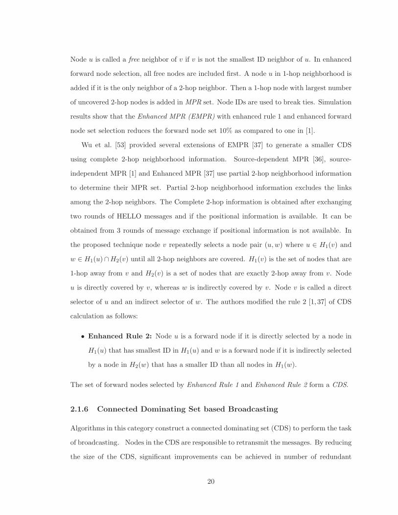
• Enhanced Rule 2: Node u is a forward node if it is directly selected by a node in
H1(u) that has smallest ID in H1(u) and w is a forward node if it is indirectly selected
by a node in H2(w) that has a smaller ID than all nodes in H1(w).
The set of forward nodes selected by Enhanced Rule 1 and Enhanced Rule 2 form a CDS.
2.1.6 Connected Dominating Set based Broadcasting
Algorithms in this category construct a connected dominating set (CDS) to perform the task
of broadcasting. Nodes in the CDS are responsible to retransmit the messages. By reducing
the size of the CDS, significant improvements can be achieved in number of redundant
20
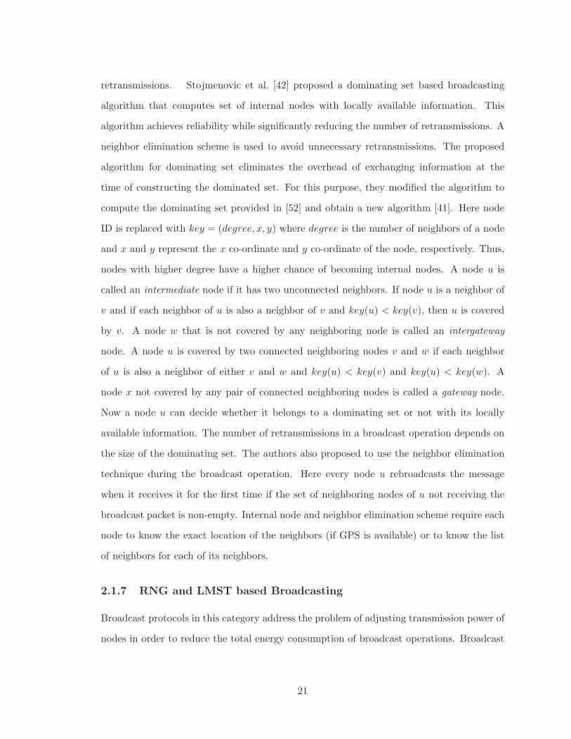
retransmissions. Stojmenovic et al. [42] proposed a dominating set based broadcasting
algorithm that computes set of internal nodes with locally available information. This
algorithm achieves reliability while significantly reducing the number of retransmissions. A
neighbor elimination scheme is used to avoid unnecessary retransmissions. The proposed
algorithm for dominating set eliminates the overhead of exchanging information at the
time of constructing the dominated set. For this purpose, they modified the algorithm to
compute the dominating set provided in [52] and obtain a new algorithm [41]. Here node
ID is replaced with key = (degree, x, y) where degree is the number of neighbors of a node
and x and y represent the x co-ordinate and y co-ordinate of the node, respectively. Thus,
nodes with higher degree have a higher chance of becoming internal nodes. A node u is
called an intermediate node if it has two unconnected neighbors. If node u is a neighbor of
v and if each neighbor of u is also a neighbor of v and key(u) < key(v), then u is covered
by v. A node w that is not covered by any neighboring node is called an intergateway
node. A node u is covered by two connected neighboring nodes v and w if each neighbor
of u is also a neighbor of either v and w and key(u) < key(v) and key(u) < key(w). A
node x not covered by any pair of connected neighboring nodes is called a gateway node.
Now a node u can decide whether it belongs to a dominating set or not with its locally
available information. The number of retransmissions in a broadcast operation depends on
the size of the dominating set. The authors also proposed to use the neighbor elimination
technique during the broadcast operation. Here every node u rebroadcasts the message
when it receives it for the first time if the set of neighboring nodes of u not receiving the
broadcast packet is non-empty. Internal node and neighbor elimination scheme require each
node to know the exact location of the neighbors (if GPS is available) or to know the list
of neighbors for each of its neighbors.
2.1.7 RNG and LMST based Broadcasting
Broadcast protocols in this category address the problem of adjusting transmission power of
nodes in order to reduce the total energy consumption of broadcast operations. Broadcast
21
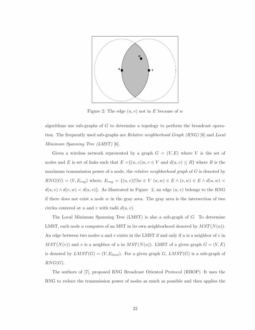
Figure 2: The edge (u, v) not in E because of w
algorithms use sub-graphs of G to determine a topology to perform the broadcast opera-
tion. The frequently used sub-graphs are Relative neighborhood Graph (RNG) [6] and Local
Minimum Spanning Tree (LMST) [6].
Given a wireless network represented by a graph G = (V,E) where V is the set of
nodes and E is set of links such that E ={(u, v)|u, v ∈ V and d(u, v) ≤ R} where R is the
maximum transmission power of a node, the relative neighborhood graph of G is denoted by
RNG(G) = (V,Erng) where, Erng = {(u, v)|!∃w ∈ V (u,w) ∈ E ∧ (v, w) ∈ E ∧ d(u,w) <
d(u, v) ∧ d(v, w) < d(u, v)}. As illustrated in Figure 2, an edge (u, v) belongs to the RNG
if there does not exist a node w in the gray area. The gray area is the intersection of two
circles centered at u and v with radii d(u, v).
The Local Minimum Spanning Tree (LMST) is also a sub-graph of G. To determine
LMST, each node u computes of an MST in its own neighborhood denoted by MST (N(u)).
An edge between two nodes u and v exists in the LMST if and only if u is a neighbor of v in
MST (N(v)) and v is a neighbor of u in MST (N(u)). LMST of a given graph G = (V,E)
is denoted by LMST (G) = (V,Elmst). For a given graph G, LMST (G) is a sub-graph of
RNG(G).
The authors of [7], proposed RNG Broadcast Oriented Protocol (RBOP). It uses the
RNG to reduce the transmission power of nodes as much as possible and then applies the
22
neighbor elimination technique to further reduce the redundant retransmissions. Experi-
mental results show that it achieves performance comparable to the best known globalized
BIP algorithm.
Cartigny et. el [6] proposed an extension of RBOP known as RBOP-T (RNG Broadcast
Oriented Protocol with Full Timeout). In RBOP, only nodes receiving a packet on non-
RNG edge apply timeout before retransmissions. In the case of RBOP-T, all nodes wait
for a fixed amount of time before retransmitting a message. They also proposed another
protocol named LBOP-T (Local MST Broadcast Oriented Protocol with Full Timeout).
This protocol first replaces RNG in RBOP with Local MST and then applies a timeout
before any node retransmits a message.
Li et al. [27] proposed a protocol named Broadcast on Local Minimum Spanning Tree
(BLMST). In this technique an LMST is constructed and a broadcast message is relayed
through the tree in constrained flooding fashion. Here if a node v receives a message from all
its neighbors in the LMST or knows that every neighbor has already received the message,
it will not relay the message. The authors argued that as the LMST provides a minimally
connected topology, applying further optimization rules to suppress the relay nodes will
lead to marginal improvement. BLMST has several desirable features. BLMST is indepen-
dent of the power consumption model. Since the LMST preserves network connectivity,
the coverage under BLMST is 100%. The control message overhead to get neighborhood
information is not significant. Moreover, BLMST is scalable with increasing values of n.
Ingelrest et al. [20] considered that the minimal transmission energy required by a node
u so that the transmission can be received successfully by a neighbor v at distance r is
proportional to rα + ce, where α is a path loss component and ce is a factor considering
the energy expenditure due signal processing, message reception, etc. They argued for the
existence of optimal radius computed with hexagonal tiling of network area, that minimizes
the energy consumption for a broadcast operation. The authors modified the existing
LBOP [6] to take advantage of the optimal radius. This new protocol is named as Target
Radius LMST Broadcast Oriented Protocol (TR-LBOP). As the node density increases,
LBOP reduces transmission radii as LMST neighbors are getting closer. Short radii cause
23

more nodes to act as relays. The constant energy charge ce for each transmission leads to
huge energy consumption. LBOP is modified so that each node increases its transmission
range up to the target optimal value when a retransmission is needed. Every node u
maintains two lists: L(u) and L′(u). L(u) contains LMST neighbors v of u and L′(u) stores
every other neighbor of u. During the neighbor elimination scheme, each neighbor v that
receives the message is removed from either L(u) or L′(u). When the timeout occurs, if
L(u) is empty, the retransmission is canceled. If there is at least one node in L(u) node u
has to rebroadcast the message to reach the nodes left in L(u). In this case, the authors
defined two values DL and DL′ where DL is the length of the furthest LMST neighbor v
from u and DL′ is the length of the edge between u and its as yet unreached neighbor w
which is closest to optimal radius T . Finally the radius of u is chosen to be the maximum
of DL and DL′ .
In Target Radius and Dominating Set Based Protocol (TRDS) [20], the radii of nodes
are reduced to the target transmission radius T . This algorithm works in three steps.
1. The topology of the network is adapted in such a way that each node selects a trans-
mission radius very close to T and still maintains connectivity. For this purpose, a
sub-graph of G is constructed where each node considers only neighbors in RNG or
LMST and the neighbors whose distance is less than or equal to T . The resulting sub
graph GT is sparse, connected and bidirectional.
2. Given a connected graph GT , a connected dominating set (CDS) is determined using
any CDS algorithm. The size of the CDS is further reduced by computing the RNG
of the graph induced by the CDS. After this, every CDS node has just to cover its
dominant neighbors in RNG.
3. For each node u, the set of CDS neighbors is denoted by ND(u) and the set of non-CDS
neighbors is denoted by ND(u). A CDS node u wishing to launch a broadcast message
emits its message with the minimal range that covers ND(u) and ND(u). A non-CDS
node v that wishes to transmit a broadcast packet transmits its message to its nearest
associated CDS neighbor u. A CDS node u receiving a message rebroadcasts it with
24

the range which allows to cover non-covered nodes in ND(u) and ND(u). A non-CDS
node v will never relay messages.
The authors argued that several localized broadcasting protocols for minimizing energy
consumption are proposed and they are based on selecting neighbors from a sparse topology.
They do not consider the constant energy charge ce for each transmission. As a result, in the
case of dense networks, these algorithms produce energy inefficient solutions. Both TRDS
and TR-LBOP algorithms are efficient and give good results as compared to BIP for all
network densities.
2.2 Broadcasting in Duty Cycled WSN
Broadcasting in wireless ad hoc networks has been intensively studied while broadcast in
duty cycled wireless sensor networks is comparatively not as well-studied in the literature.
We classified the broadcast algorithms for duty cycled WSNs into two categories: centralized
and distributed. We first review the centralized algorithms in the following section and then
discuss distributed algorithms in section 2.2.2.
2.2.1 Centralized Algorithms
Gu et al. [11] proposed the Dynamic Switch Forwarding (DSF) technique for low duty-cycle
sensor networks with unreliable links in order to achieve optimal expected delivery ratio,
expected end-to-end delay and expected energy consumption. In duty cycled networks, link
quality-based forwarding techniques suffer from high end-to-end delay due to sleep latency.
On the other hand, sleep latency based forwarding techniques suffer from high end-to-end
delay due to the change of link quality. In DSF, given a sink, each node maintains a sequence
of forwarding nodes that are sorted in the order of the wake-up time associated with them.
To send a packet, a node scans the first node in the forwarding sequence as it will wake
up soon and tries to send the packet. If the transmission is successful then the node stops.
If it is unsuccessful, the node fetches the next node from the sequence and tries to send
the packet again. The advantage of this technique is that it reduces the time spent on
25
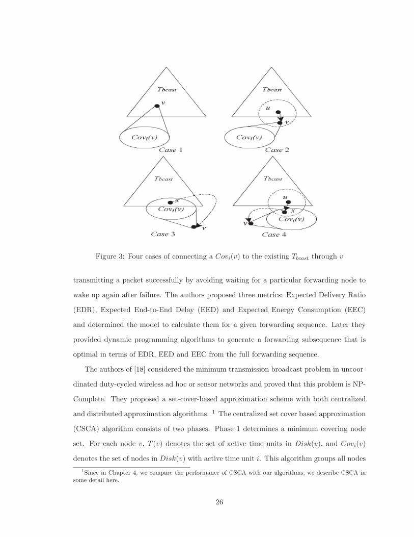
Figure 3: Four cases of connecting a Covi(v) to the existing Tbcast through v
transmitting a packet successfully by avoiding waiting for a particular forwarding node to
wake up again after failure. The authors proposed three metrics: Expected Delivery Ratio
(EDR), Expected End-to-End Delay (EED) and Expected Energy Consumption (EEC)
and determined the model to calculate them for a given forwarding sequence. Later they
provided dynamic programming algorithms to generate a forwarding subsequence that is
optimal in terms of EDR, EED and EEC from the full forwarding sequence.
The authors of [18] considered the minimum transmission broadcast problem in uncoor-
dinated duty-cycled wireless ad hoc or sensor networks and proved that this problem is NP-
Complete. They proposed a set-cover-based approximation scheme with both centralized
and distributed approximation algorithms. 1 The centralized set cover based approximation
(CSCA) algorithm consists of two phases. Phase 1 determines a minimum covering node
set. For each node v, T (v) denotes the set of active time units in Disk(v), and Covi(v)
denotes the set of nodes in Disk(v) with active time unit i. This algorithm groups all nodes
1Since in Chapter 4, we compare the performance of CSCA with our algorithms, we describe CSCA insome detail here.
26
with active time slot i in G(V,E) into sets Ui and tries to find a minimum covering node
set Ci for each Ui in a greedy fashion so that ∪v∈CiCovi(v) = Ui. Phase 2 then constructs a
backbone structure by connecting all ∪i∈TCi to s through some connectors. The backbone
is determined during the formation of a spanning tree Tbcast on G. Initially, Tbcast starts
with s and a working set Temp is set to ∪i∈TCi. This phase scans all the element in Temp
and selects the first Covi(v) satisfying one of the following conditions as shown in Figure
3 and takes appropriate action:
1. v is in Tbcast; In this case no operation is required.
2. v is adjacent to some u in Tbcast; In this case connect u to v.
3. A node x belongs to Covi(v) ∩ Tbcast; In this case connect x to v.
4. A node x in Covi(v) is adjacent to some u ∈ Tbcast; In this case connect x to u and x
to v.
Node v is removed from Temp if all Covi(v) for i ∈ T are processed. This process
continues until Temp is empty.
The approximation ratio of the CSCA algorithm is shown to be 3(ln(Δ) + 1), where
Δ is the maximum degree of the network. The time complexity of the CSCA algorithm is
O(n3).
In [46], the broadcast problem in a duty cycled wireless sensor network is considered
as a shortest path problem in a time-coverage graph and an energy efficient centralized
algorithm that utilizes dynamic programming is proposed. This algorithm saves energy by
minimizing forwarding cost and delay. In this algorithm, at first a time-coverage graph is
constructed. If a set R of nodes receive a message at time t, it is represented as a vertex vR,t
in the time-coverage graph. R starts with {s} and gradually becomes {1, 2, 3, ...., n}. Thereare two kinds of edges: time edges and forward edges. If nodes of R do not forward messages
at t, then same coverage state will exist in next time slot. This situation is depicted by a
time edge that connects neighboring vertices along a row from earlier to later. A forwarding
edge represents a forwarding event. A forwarding edge from vR,t to vR′,t′ indicates that at
27
time t, one or more nodes in R transmit a message. The weight of an edge is a combination
of message and time cost. When the weight of a time edge is calculated it emphasizes on
the delay and the number of messages forwarded by the nodes in R is highlighted during
the calculation of the weights of forward edges. Let W (vR,t, vR′,t′) denote the weight of an
edge from vR,t to vR′,t′ and W (vR,t, vR′,t′) = ∞ if no such edge exists. F (vR′,t′) is the total
weight of the shortest path from vs,t0 to vR′,t′ . F (vR′,t′) is calculated as follows:
F (vR′,t′)=minvR,t(F (vR,t)+W (vR,t, vR′,t′))
where F (vs,t0) = 0 and F (vR,t0) = ∞ for R �= s. With the above relation and the boundary
values, the weight of the shortest path from vs,t0 to each vertex from top to bottom and
for each row, from left to right can be calculated. The minimum of the total weights to the
last-row vertices is the weight of the shortest path from vs,t0 to a vertex in last row.
The problem of finding energy-efficient sleep scheduling that will optimize the end-to-end
delay is addressed in [31]. The authors made an attempt to minimize the communication
latency when each sensor has a duty cycling requirement of being awake for only 1/k time
slots on an average. As a first step, they considered each sensor can be active in exactly one
time unit among the k slots. They proved that finding a sleep scheduling that will minimize
the end to end communication delay in a network with all-to-all communication flow and
weighted communication flow is generally NP-hard. They found that an optimal solution
can be obtained for two special cases of all-to-all communications: tree topologies and ring
topologies. They proposed several heuristics for networks with all-to-all communication
patterns. In the centralized algorithm, initially all nodes are assigned same slots. Each node
calculates the delay diameter D for all possible slot assignments for itself while keeping the
time slots for other nodes fixed. The minimum of the delay diameters of all possible slot
assignments is denoted by dmin. If dmin is smaller than the previous delay diameter d, the
node changes its slot to the one with minimum D and updates d to dmin. After all nodes
perform the operation, the iteration can be repeated. The number of iterations depends on
the time limitation of the algorithm.
The authors of [17] investigated the problem to find a broadcast schedule that avoids
28
collisions and minimizes the broadcast latency in a duty cycled wireless ad hoc network and
they proved that this problem is NP-Complete. They proposed two approximation algo-
rithms named Simple Layered Coloring Algorithm (SLAC) and Enhanced Layered Coloring
Algorithm (ELAC). Both of the two algorithms construct a broadcast tree using Dijkstra’s
algorithm for shortest paths where the cost of an edge λ(u, v) is defined as follows:
λ(u, v) =
⎧⎪⎨⎪⎩
|T | if SLa(v) = SLa(u)
(SLa(v)− SLa(u) + |T |) mod |T |, otherwise
where, SLa(u) and SLa(v) represent the active time slot of node u and v respectively
and T is the length of the wake up schedule.
If a node u in the constructed tree has a receiving time slot SLr(u) = k|T | + i, it is
considered as a node at layer k|T |+ i. The maximum k is denoted by K and the maximum
i is denoted by I and the maximum layer is denoted by K|T | + I. Collisions will occur
only when two or more nodes transmit to nodes in the same layer p on the tree at the same
time. SLAC schedules the the parents of nodes in layer p to transmit in different time. For
this purpose this algorithm utilizes the D2-coloring scheme. In D2-coloring scheme, no two
vertices having distance 1 or 2 will not be assigned the same color [39]. The approximation
ratio of SLAC is O(Δ2 + 1), where Δ is the maximum degree of the network.
ELAC improves the SLAC algorithm by dividing the transmissions on each layer into
two phases. Let Up denotes the set of nodes on layer p. ELAC constructs the Maximal
Independent Set (MIS) Ap for each Up. This algorithm finds a proper D- coloring of Ap. It
finds the transmissions from the parents of Ap to the nodes in Ap and schedules transmissions
from Ap to the nodes in Up. The approximation ratio of ELAC is 24|T |+1 where |T | is thenumber of time slots in a scheduling period.
The One-to-All-Broadcast (OTAB) algorithm is proposed in [22]. This algorithm re-
duces the broadcast latency and provides a collision free broadcast schedule. As in SLAC
and ELAC, this algorithm also builds a shortest path tree with root at s using Dijkstra’s
algorithm. OTAB assumes that s starts the broadcast operation at time slot 0. For every
edge (u, v), the latency Lat(u, v) is defined as follows:
29
Lat(u, v) =
⎧⎪⎪⎪⎪⎪⎨⎪⎪⎪⎪⎪⎩
A(v) + 1, if u = s;
A(v)−A(u), if u �= s and A(v)−A(u) > 0;
A(v)−A(u) + |T |, otherwise
OTAB constructs a broadcast tree TB based on the shortest path tree and schedules the
broadcast accordingly. All the nodes in V are grouped into different layers L0, L1, . . . , LD
according to their latency of the shortest paths from s, where D is the maximum latency of
all the shortest paths. Nodes at the same layer Li have the same active time slot. All the
nodes except s are divided into different sets U0, U1, U2, . . . , U|T |−1 according to their active
time slots. For each Uj , 1 ≤ j ≤ |T | − 1, OTAB determines an MIS Qj . All the nodes at
Li, 0 ≤ i ≤ |T |− 1 are divided into two sets: an Independent Set(IS) Mi and Li \Mi, where
Mi ∈ Qj and j equals (i − 1) mod |T |. Each Uj is divided into two sets Qj and Uj \ Qj .
Now TB is constructed using a layered approach. At each Li, the parent nodes of Mi are
chosen from some nodes at higher layers. Some nodes of Mi are selected as the parents of
nodes in Li \Mi and nodes at lower layers with the same active time slot. Then for each
Uj , 1 ≤ j ≤ |T | − 1, parents of Qj and Uj \ Qj are colored using D2- coloring methods.
Transmissions from the parent nodes to their children nodes are scheduled based on the
colors of the parent nodes. This scheduling starts at time slot 0. At each layer Li, the
transmissions from the parent nodes for each node u ∈ Mi are scheduled and finally the
transmissions from the parent node of each w in Li \Mi are scheduled based on the coloring
of the nodes. The approximation ratio of OTAB is at most 17|T | where |T | is the number
of time slots in a scheduling period.
We compare the results of our algorithms with the existing algorithms CSCA [18] and an
adapted version of OTAB [22] named SDT(Shortest Delay Tree). We eliminate the phase
of resolving collisions from OTAB for the purpose of fair comparison with our proposed
algorithms.
30

2.2.2 Distributed Algorithms
Gu et al. proposed the distributed version of DSF in [11]. The centralized version of the
algorithm is discussed in Section 2.2.1. Initially, the sink node knows the values of EDR,
EED and EEC and it is 1 for EDR, 0 for EED and EEC. The distributed DSF algorithm
starts working by allowing the sink node to broadcast its EDR, EED and EEC values.
When a node receives these information it starts to calculate its own EDR, EED and EEC
utilizing the received information and determines the forwarding set for itself that optimizes
a particular metric using the proposed dynamic algorithms. If the change in new values of
EDR, EED and EEC exceeds a certain threshold compared to the old values of EDR, EED
and EEC, the node will broadcast the new values. This process continues at a node until it
does not receive any information about the updated expected values from all its neighbors.
The authors of [12] proposed a distributed flooding scheme for low-duty cycle wireless
sensor networks with unreliable communication links. They constructed an energy optimal
tree to reduce transmission redundancies and dissemination delay. The energy optimal tree
is constructed by allowing a smaller hop count node to transmit to a larger hop count
node, where every node selects only one incoming link that has the best link quality among
all its incoming links. These best quality links reduce the number of collisions as well as
retransmissions of messages. The authors proposed a recursive equation to compute the
distribution of forwarding delay for each node in a distributed way. From this a node u
determines its p-quantile delay Dp as its threshold value and shares it with all the neighbors.
If a node v has a packet to forward to u, it calculates Expected Packet Delay (EPD) and
compares with Dp. If EPD < Dp, the packet is delivered to u. In this way, a node u in
the tree can receive a packet from v that is not its parent in the tree as v can deliver the
packet faster than u’s parent. As the forwarding decision is distributed, it may happen that
two or more nodes decide to transmit to a single node and the sending nodes cannot hear
each other. To solve this problem a sender set for a given node is constructed where all
nodes can hear each other to avoid collision and a back off technique is proposed to avoid
collisions among the nodes in the sender set. Opportunistic flooding achieves significantly
31
shorter flooding delay and consumes less transmission energy as compared to an improved
version of traditional flooding implemented in duty cycled wireless sensor networks.
An adaptive algorithm to dynamically schedule message forwarding is proposed in [45].
It utilizes only local topology information and does not depend on global synchronization.
It exploits overhearing to reduce message costs. This algorithm obtains near-optimal per-
formance in terms of time and message costs and achieves high reliability.
Hong et al. [18] proposed the distributed version of CSCA algorithm described in 2.2.1.
In Distributed Set Covered Approximation (DSCA) algorithm every node is initially in idle
listening state and turns to duty-cycling mode when a trigger variable z is set from 0 to 1.
An i-dominator is a covering node for Ui and an i-dominatee is a node in Ui covered by
some i-dominator. The authors used the term ∗-dominator and ∗-dominatee to represent
any i-dominator and i-dominatee. In order to distributively implement the algorithm, the
i-dominator is elected from Ui. Each node has its 2-hop neighbor information. Initially,
all nodes are marked in white and then turned to blue if they become i-dominators or i-
dominatees. Every white node with active time slot i broadcasts the IamDominator(ID, i)
message and is marked blue if it has the most white neighbor nodes with active time
slot i among all its 1-hop white neighbors. A white node with active time slot i also
becomes an i-dominator and is marked blue if it has neither white neighbors with active
time slot i nor i-dominators. A white node with active time slot i becomes an i-dominatee
and is marked blue when it receives IamDominator(ID, i) message and broadcasts the
IamDominatee(ID, i) message. At the end, each node is a ∗-dominator or a ∗-dominatee
and all nodes in Ui are covered by i-dominators.
Next phase determines the connections among i-Dominators and s. A forwarding tree
H connecting all i-dominators and s is constructed by exchanging the INV/JOIN messages
for all i ∈ T . Each node maintains a local trigger variable z that is set from 0 to 1 after this
node joins H. The approximation ratio of the DSCA algorithm is a constant of at most
20. Both the time and the message complexities of the DSCA algorithm are O(n).
The Asynchronous Duty-Cycle Broadcasting (ADB) protocol for wireless sensor net-
works using asynchronous duty cycling is proposed in [43]. This protocol is integrated with
32
MAC layer to utilize the information available at this layer. It optimizes broadcast op-
eration at level of individual transmission of a node to a neighbor. ADB utilizes unicast
transmission to every neighbor and waits for an acknowledgment from the receiving node.
It uses a receiver- initiated mechanism to prevent a node from occupying the medium for
too long a time. Whenever a neighbor wakes up, it sends a beacon message. After receiving
the beacon message the node can send the data packet. While a node is waiting for the
beacon before transmitting data, the medium can be utilized by the neighbors of the node
that already received the packet to transmit to their neighbors in order to reduce delivery
latency. ADB efficiently incorporates the progress of broadcast operation with the data
packet to reduce number of transmissions by a node. It makes use of the best quality link
to reduce energy consumption, delivery latency and to increase delivery ratio.
Thus ADB has certain properties making it energy efficient, reduce delivery latency and
increase delivery ratio. They are:
1. ADB allows a node to go to sleep as soon as all its neighbors are reached or delegated
to other nodes.
2. It avoids transmissions on poor links.
3. It prevents a node to occupy the medium for long time.
4. When a node wakes up, it is informed about the progress of broadcast with the data
packet to avoid unnecessary waiting and transmissions.
The authors confirmed through experiments that ADB is highly energy efficient, reduces
network load and delivery latency while achieving 99% delivery ratio.
Wang et al. [46] proposed the distributed version of finding shortest path in time-
coverage graph. The centralized version of the algorithm is discussed in 2.2.1. From
the solution of the centralized algorithm the authors derived an efficient and scalable dis-
tributed algorithm that utilizes local information and is associated with loss compensation
techniques. For each sensor node this algorithm will determine the optimal forwarding
sequence covering its 2-hop neighbors. Each node w determines CovSet consisting of its
33
1-hop and 2-hop neighbors known by w being covered by at least one forwarding. When
w forwards a message or overhears a neighbor is doing so will update the CovSet. The
centralized dynamic programming algorithm is modified so that every node w starts from
the row with index equal to its CovSet and the index of the last row will contain only the
node w and its 1- and 2-hop neighbors.
From simulations it is observed that the distributed algorithm achieves a near optimal
performance and its time cost as well as the message cost is very close to the lower bound
of the time cost and the message cost. Its computation and control overheads both scale
well with the network size and density. It is also robust against wireless losses and cope
well with different duty-cycles.
Stann et al. [40] proposed the Robust Broadcast Protocol (RBP) to improve the relia-
bility of the broadcast operation while maintaining energy efficiency. This protocol requires
only local information. It makes a single broadcast more reliable and hence decreases the
frequency with which an upper layer protocol needs to invoke flooding. Thus better reli-
ability of the broadcast operation improves the energy consumption. In RBP, every node
knows its 1-hop neighbors. RBP generates a unique identifier when a new broadcast mes-
sage is initiated. It must understand when broadcasts by different nodes correspond to the
same flood. When a node hears a broadcast for the first time, it retransmits the packet
unconditionally. When other neighbors also transmit the same packet, the node keeps track
of which neighbors have broadcasted the packet. RBP considers the transmission by a
neighbor as an implicit ACK. When the number of implicit ACKs observed by a node falls
below a predetermined threshold, a node will again retransmit the packet. A receiver also
sends an explicit unicast ACK when it hears a repeated broadcast from the same sender.
RBP can switch a node from broadcast mode to unicast in order to reduce the number of
packet transmissions. RBP adjusts both the retransmission thresholds and the number of
retries based on neighborhood density. Higher density in the neighborhood implies lower
thresholds and fewer retries as other neighbors are likely to broadcast the same packet.
RBP can identify important links that bridge between dense clusters of nodes with sparse
area of nodes. Often there can be a node v at the edge of the dense area with large number
34
of neighbors but v alone provides traffic to the sparse area. RBP identifies such links and
always ensures reliability for these links.
Experimental results show 99.8% reliability is achieved with overhead less than 48% as
compared to the level of flooding required to get the same reliability.
Lu et al. [31] proposed two localized algorithms to find a sleep schedule that will minimize
end-to-end delay in networks with all-to-all communications. In the first algorithm, a node
only knows the slot assignments of its immediate neighbors and selects one slot for itself that
will minimize the maximum delay to and from its 1-hop neighbors. This process is repeated
several times. The second algorithm works in similar fashion as the Distance Vector routing
technique. Each node maintains a forward vector table FDV which stores its shortest delays
to all other nodes and a backward table BDV which stores its shortest delays from all other
nodes. These two tables can be calculated using the basic Bellman-Ford technique. A sensor
node knows the DV tables of its immediate neighbors and calculates the DV tables for all
possible new slot assignments for itself. The maximum value of entries in the sets of the
two DV tables over all possible slot assignments is denoted by maxd. The node selects the
slot which gives the minimum maxd. In the randomized algorithm, a slot for each node
is selected randomly and the delay diameter of the network is determined. After a fixed
number of iterations, every node selects a time slot that gives the minimum delay diameter.
The proposed heuristics are evaluated through simulations. It is found that the performance
of the localized heuristics is worse than the above simple randomized slot allocations, while
the centralized scheme provides more delay reductions over randomized schemes.
2.2.3 Differences with Our Work
Due to energy constrained nature of WSNs, broadcast algorithms for the duty cycled wireless
sensor networks mainly focus on reducing the energy consumption. Various algorithms
put emphasis on various aspects in order to achieve this goal. The Algorithm in [18]
minimizes the number of node transmissions in uncoordinated duty cycled WSNs, while
the algorithm in [46] converts the broadcast problem into a shortest path problem in time-
coverage graph and saves energy by reducing forwarding cost and delay. The authors of [12]
35

reduces transmission redundancies and dissemination delay by building an energy optimal
tree where every node selects the best quality link with its parent in the tree. They also
provide a technique to avoid collisions. The ADB algorithm in [43] achieves energy efficiency
by allowing a node to go back to sleep as soon as all it neighbors are reached or delegated to
other node. Here a node remains active after receiving a packet until it goes back to sleep.
SLAC [17], ELAC [17] and OTAB [22] provide a collision free broadcast schedule that will
minimize the broadcast latency.
None of the above algorithms for duty cycled wireless sensor networks consider the issue
of minimizing the total number of additional active time units that nodes of a network
need to be active in order to accomplish the broadcast operation. In our work we prove
that the problem of reducing the total additional active time units for broadcast operation
is NP-Complete and we propose two polynomial time heuristic algorithms to address this
problem.
36
Chapter 3
Algorithms and NP-Completeness
Energy efficient broadcast operation in duty cycled WSNs can be achieved by reducing the
total number of additional active time units that the nodes of a network must be awake to
complete the broadcast operation. We call the problem of minimizing the total number of
additional active time units to accomplish a broadcast operation in a duty cycled WSN as
the Minimum Energy Broadcast Tree (MEBT) problem. We prove that the MEBT problem
is NP-Complete and propose two polynomial time heuristic algorithms to find suitable
solutions for it.
In this chapter we first present the NP-Completeness proof of MEBT problem that is
followed by the heuristic algorithms to address the MEBT problem. All of the algorithms
construct a spanning tree rooted at a source node to accomplish the broadcast operation
by minimizing the total additional active time units.
3.1 Definitions and Preliminaries
A Duty Cycled WSN is a triple G = (V,E,M) where V is the set of nodes in the network,
E ⊆ V × V is the set of links and Mu is the Wakeup Schedule of node u and is a binary
37

array of length n where,
Mu[i] =
⎧⎪⎨⎪⎩
1 if node u is in active state in time unit i
0 otherwise
Our goal is to provide broadcast service with minimum energy consumption in duty cycled
WSNs. To accomplish this task usually a broadcast tree is constructed. A broadcast tree is
a directed spanning tree rooted at a source node such that a packet from the source node
can be sent to every other node in the network using the edges of the tree. Since a parent
node has to stay awake until it delivers the packet to all its children in the tree, the number
of active time units for the parent node is usually greater than that specified in its wakeup
schedule.
In other words, the broadcast tree dictates a new schedule for each node, which we call
the Broadcast Schedule. The broadcast schedule of a node is a binary array B of length nd
where, d is the depth of the tree. Let the extended wakeup schedule of a node be specified
by an array M ′u of size nd, which consists of d consecutive copies of the wakeup schedule;
this specifies when the nodes would be awake in a time period of nd according to their
wakeup schedules. Suppose a node u receives the broadcast packet at time t0 and it has k
children in the broadcast tree. Let ti be the next time unit when a child vi is awake, then
the number of time units u will remain active is max{ti − t0|1 ≤ i ≤ k}. The broadcast
schedule for u is defined as follows:
BT (u, t) =
⎧⎪⎨⎪⎩
1 if t0 ≤ t ≤ max1≤i≤kti
M ′u(t) otherwise
It is easy to see that a parent delivers a packet to all its children within n time units after
receiving it. Clearly for any node u,∑nd
i=0BT (u, i) ≥ ∑ndi=0M
′u[i]. We define the cost of a
broadcast tree T to be cost(T ) =∑N
u=1
∑ndi=0(BT (u, i) − M ′
u[i]). In other words, the cost
of a broadcast tree is the total number of additional time units that the nodes in the tree
remain awake in order to accomplish the broadcast. The problem that we are interested
in is the Minimum Energy Broadcast Tree (MEBT) problem, that is: Given a duty cycled
38
network G = (V,E,M) and a source node s ∈ V , find a broadcast tree T rooted at s for G
such that cost(T ) ≤ cost(T ′) for all broadcast trees T ′ for G.
In our experiments, we also consider additional cost measures that have been studied
previously such as the minimum number of node transmissions, the maximum delay and
average delay dictated by a broadcast tree.
3.2 NP-Completeness of MEBT Problem
In this section, we show that the decision version of the MEBT problem is NP-Complete.
Theorem 1. Given a duty cycled wireless sensor network G = (V,E,M) and a source node
s ∈ V , the problem of determining if there exists a broadcast tree for G rooted at s with cost
at most W is NP-complete.
Proof. Given a candidate broadcast tree T rooted at a source node, we can calculate the
cost and check whether it is greater than W in polynomial time. So the problem is in NP.
We consider a special case of the problem, where the wakeup schedule of each node consists
of 2 time units. We will show that the problem is NP-complete for this special case by
reducing the 1-in-3 SAT problem to it and thus also NP-complete for more general case.
Let the 1-in-3 SAT instance consist of n boolean variables x1,x2,. . . ,xn and m clauses
C1,C2,. . . ,Cm where Cj = yj,1∨yj,2
∨yj,3 and the three literals yj,1,yj,2,yj,3 ∈ {x1, x1, x2, x2
. . . , xn, xn}, 1 ≤ j ≤ m. If the instance is satisfiable, then in each clause Cj , exactly one
of yj,l is true, while the other two literals are false, 1 ≤ j ≤ m, 1 ≤ l ≤ 3. We construct
the MEBT instance G = (V,E,M) corresponding to this 1-in-3 SAT instance. The vertices
and their wakeup schedules are specified as follows:
• There is a source node S0,0 where MS0,0 [1] = 1 and MS0,0 [2] = 0.
• For each boolean variable xi there are two corresponding nodes Si,1 and Si,2 and
MSi,j [1] = 1 and MSi,j [2] = 0, where, 1 ≤ i ≤ n, 1 ≤ j ≤ 2.
• For each boolean variable xi there is an additional node Xi with MXi [1] = 0 and
MXi [2] = 1, where, 1 ≤ i ≤ n.
39
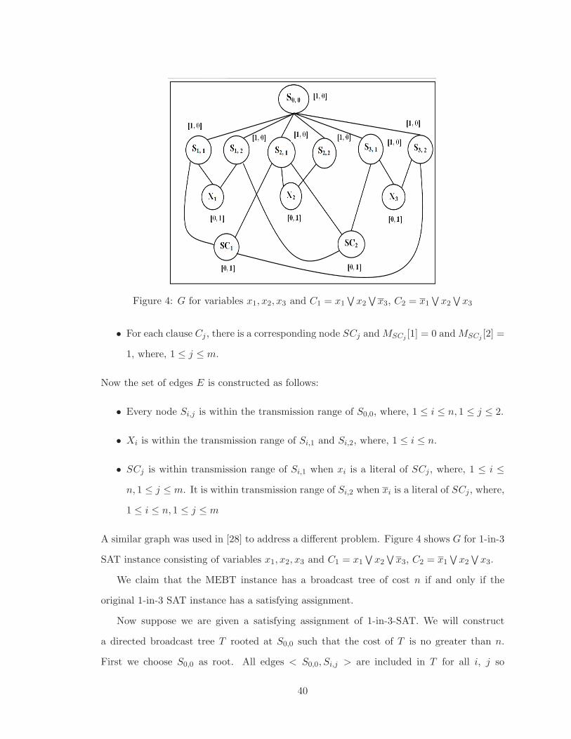
Figure 4: G for variables x1, x2, x3 and C1 = x1∨x2
∨x3, C2 = x1
∨x2
∨x3
• For each clause Cj , there is a corresponding node SCj andMSCj [1] = 0 andMSCj [2] =
1, where, 1 ≤ j ≤ m.
Now the set of edges E is constructed as follows:
• Every node Si,j is within the transmission range of S0,0, where, 1 ≤ i ≤ n, 1 ≤ j ≤ 2.
• Xi is within the transmission range of Si,1 and Si,2, where, 1 ≤ i ≤ n.
• SCj is within transmission range of Si,1 when xi is a literal of SCj , where, 1 ≤ i ≤n, 1 ≤ j ≤ m. It is within transmission range of Si,2 when xi is a literal of SCj , where,
1 ≤ i ≤ n, 1 ≤ j ≤ m
A similar graph was used in [28] to address a different problem. Figure 4 shows G for 1-in-3
SAT instance consisting of variables x1, x2, x3 and C1 = x1∨x2
∨x3, C2 = x1
∨x2
∨x3.
We claim that the MEBT instance has a broadcast tree of cost n if and only if the
original 1-in-3 SAT instance has a satisfying assignment.
Now suppose we are given a satisfying assignment of 1-in-3-SAT. We will construct
a directed broadcast tree T rooted at S0,0 such that the cost of T is no greater than n.
First we choose S0,0 as root. All edges < S0,0, Si,j > are included in T for all i, j so
40
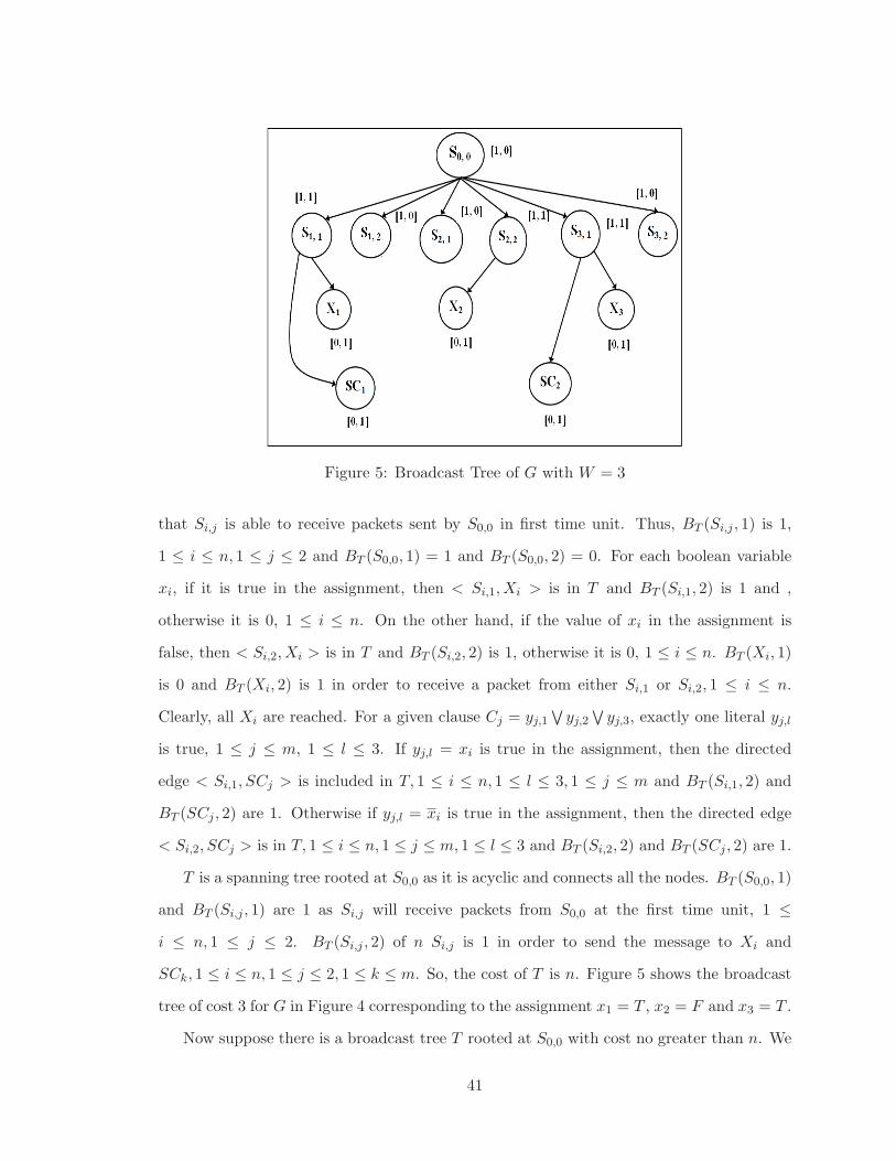
Figure 5: Broadcast Tree of G with W = 3
that Si,j is able to receive packets sent by S0,0 in first time unit. Thus, BT (Si,j , 1) is 1,
1 ≤ i ≤ n, 1 ≤ j ≤ 2 and BT (S0,0, 1) = 1 and BT (S0,0, 2) = 0. For each boolean variable
xi, if it is true in the assignment, then < Si,1, Xi > is in T and BT (Si,1, 2) is 1 and ,
otherwise it is 0, 1 ≤ i ≤ n. On the other hand, if the value of xi in the assignment is
false, then < Si,2, Xi > is in T and BT (Si,2, 2) is 1, otherwise it is 0, 1 ≤ i ≤ n. BT (Xi, 1)
is 0 and BT (Xi, 2) is 1 in order to receive a packet from either Si,1 or Si,2, 1 ≤ i ≤ n.
Clearly, all Xi are reached. For a given clause Cj = yj,1∨yj,2
∨yj,3, exactly one literal yj,l
is true, 1 ≤ j ≤ m, 1 ≤ l ≤ 3. If yj,l = xi is true in the assignment, then the directed
edge < Si,1, SCj > is included in T, 1 ≤ i ≤ n, 1 ≤ l ≤ 3, 1 ≤ j ≤ m and BT (Si,1, 2) and
BT (SCj , 2) are 1. Otherwise if yj,l = xi is true in the assignment, then the directed edge
< Si,2, SCj > is in T, 1 ≤ i ≤ n, 1 ≤ j ≤ m, 1 ≤ l ≤ 3 and BT (Si,2, 2) and BT (SCj , 2) are 1.
T is a spanning tree rooted at S0,0 as it is acyclic and connects all the nodes. BT (S0,0, 1)
and BT (Si,j , 1) are 1 as Si,j will receive packets from S0,0 at the first time unit, 1 ≤i ≤ n, 1 ≤ j ≤ 2. BT (Si,j , 2) of n Si,j is 1 in order to send the message to Xi and
SCk, 1 ≤ i ≤ n, 1 ≤ j ≤ 2, 1 ≤ k ≤ m. So, the cost of T is n. Figure 5 shows the broadcast
tree of cost 3 for G in Figure 4 corresponding to the assignment x1 = T , x2 = F and x3 = T .
Now suppose there is a broadcast tree T rooted at S0,0 with cost no greater than n. We
41

want to show that we can derive a satisfying assignment for the 1-in-3 SAT instance. First
observe that since T is a directed spanning tree, and since every Xi is connected only to
Si,1 and Si,2 in the graph, exactly one of the links (Si,1, Xi) and (Si,2, Xi) must be present
in the tree, where 1 ≤ i ≤ n. Since both Si,1 and Si,2 are only awake in the first time unit,
and Xi only in the second, the presence of these links alone gives a cost of n to the tree.
Therefore, any other links in the tree must come for free; they must not add any cost to the
tree. Therefore, the parent of any node SCj in the tree must be a node Si,1 or Si,2 that is
also the parent of its corresponding Xi, where 1 ≤ i ≤ n,1 ≤ j ≤ m. That is, if (Si,1, SCj)
is a link in the tree, then (Si,1, Xi) is present as well.
To obtain a satisfying assignment now is easy. For each i, if (Si,1, Xi) is in the tree,
then the corresponding variable xi in the 1-in-3 SAT instance is assigned the value True,
otherwise (Si,2, Xi) is in the tree, and xi is assigned the value False, 1 ≤ i ≤ n. Clearly this
is a valid assignment. Finally, since T is a directed spanning tree, every SCj has exactly
one incoming link, 1 ≤ j ≤ m. If the incoming link is from a node Si,1, then the literal xi
is in the clause Cj , 1 ≤ i ≤ n, 1 ≤ j ≤ m. Recall that in this case, the edge it has been
assigned the value True, the clause will be satisfied. On the other hand, if the incoming
link is from a node Si,2, then the literal xi is in the clause Cj , 1 ≤ i ≤ n, 1 ≤ j ≤ m. Since
in this case, the variable xi has been assigned False, the clause will be satisfied. Thus we
have a satisfying assignment with exactly one true literal per clause as required.
3.3 Algorithms
In this section we present our polynomial time algorithms to find a broadcast tree with low
cost. We will use a simple duty cycled WSN G to describe the operation of our proposed
algorithms. The duty cycled WSN G used for this purpose is shown in Figure 6. It consists
of 11 nodes. The length of the wakeup schedule is 6 and every node is active for exactly
one time unit in this schedule. The nodes are labeled starting from a. We select node a as
the source node responsible for initiating the broadcast operation.
42
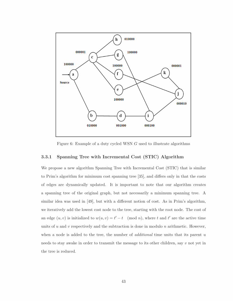
Figure 6: Example of a duty cycled WSN G used to illustrate algorithms
3.3.1 Spanning Tree with Incremental Cost (STIC) Algorithm
We propose a new algorithm Spanning Tree with Incremental Cost (STIC) that is similar
to Prim’s algorithm for minimum cost spanning tree [35], and differs only in that the costs
of edges are dynamically updated. It is important to note that our algorithm creates
a spanning tree of the original graph, but not necessarily a minimum spanning tree. A
similar idea was used in [49], but with a different notion of cost. As in Prim’s algorithm,
we iteratively add the lowest cost node to the tree, starting with the root node. The cost of
an edge (u, v) is initialized to w(u, v) = t′ − t (mod n), where t and t′ are the active time
units of u and v respectively and the subtraction is done in modulo n arithmetic. However,
when a node is added to the tree, the number of additional time units that its parent u
needs to stay awake in order to transmit the message to its other children, say v not yet in
the tree is reduced.
43
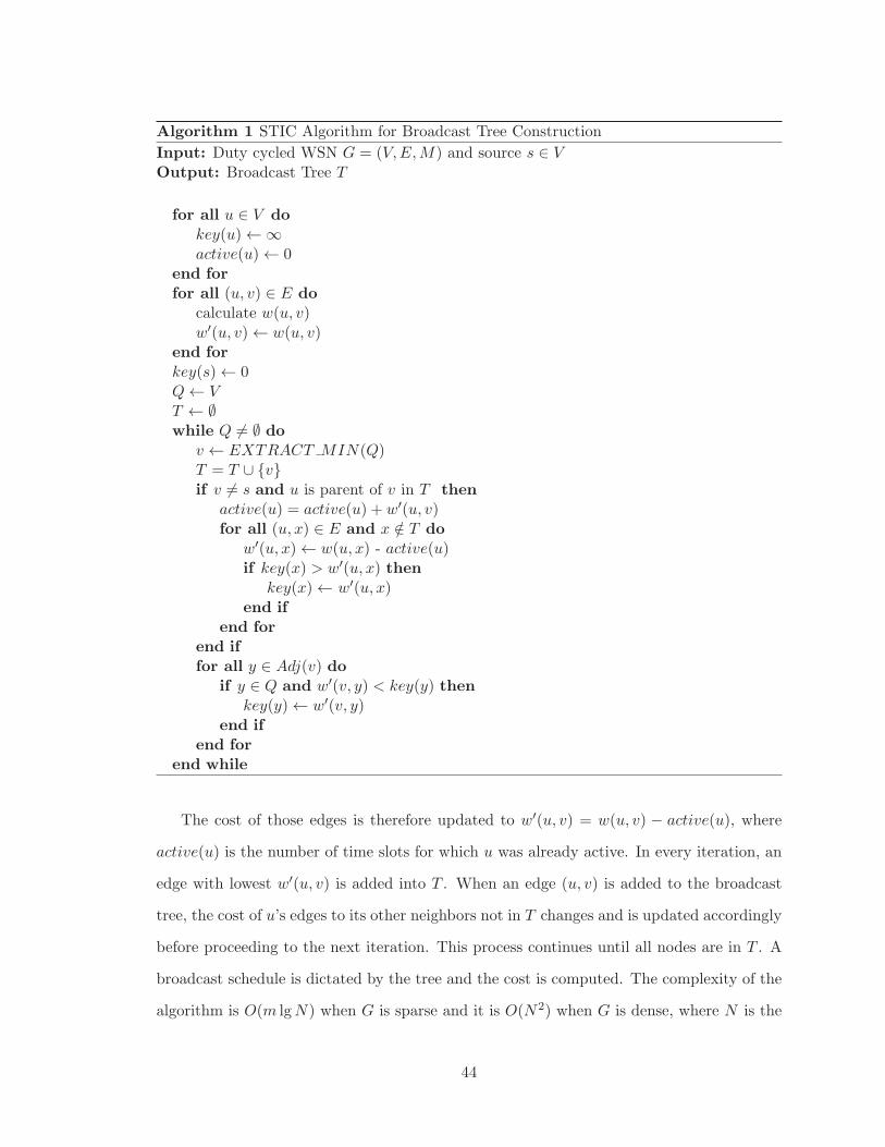
Algorithm 1 STIC Algorithm for Broadcast Tree Construction
Input: Duty cycled WSN G = (V,E,M) and source s ∈ VOutput: Broadcast Tree T
for all u ∈ V dokey(u) ← ∞active(u) ← 0
end forfor all (u, v) ∈ E do
calculate w(u, v)w′(u, v) ← w(u, v)
end forkey(s) ← 0Q ← VT ← ∅while Q �= ∅ do
v ← EXTRACT MIN(Q)T = T ∪ {v}if v �= s and u is parent of v in T then
active(u) = active(u) + w′(u, v)for all (u, x) ∈ E and x /∈ T do
w′(u, x) ← w(u, x) - active(u)if key(x) > w′(u, x) then
key(x) ← w′(u, x)end if
end forend iffor all y ∈ Adj(v) do
if y ∈ Q and w′(v, y) < key(y) thenkey(y) ← w′(v, y)
end ifend for
end while
The cost of those edges is therefore updated to w′(u, v) = w(u, v) − active(u), where
active(u) is the number of time slots for which u was already active. In every iteration, an
edge with lowest w′(u, v) is added into T . When an edge (u, v) is added to the broadcast
tree, the cost of u’s edges to its other neighbors not in T changes and is updated accordingly
before proceeding to the next iteration. This process continues until all nodes are in T . A
broadcast schedule is dictated by the tree and the cost is computed. The complexity of the
algorithm is O(m lgN) when G is sparse and it is O(N2) when G is dense, where N is the
44

number of nodes and m is the number of edges.
On our example network of Figure 6, STIC starts with node a and constructs T in a
number of steps. The construction of T is shown in Figures 7, 8, 9, 10, 11 and 12.
To conveniently illustrate the procedure to generate the tree, each node u is labeled with
key(u)/active(u) inside the circle whereas each edge (u, v) is labeled with w(u, v)/w′(u, v).
A bold directed arrow from u to v indicates that (u, v) is included into T . The construction
process is described below:
1. In Figure 7(b), initially key(a) = 0 and thus node a is added into T . Node b and
c are adjacent to a and key(c) and key(b) are updated to 5 and 1, respectively as
w(a, b) = w′(a, b) = 1 and w(a, c) = w′(a, c) = 5.
2. As shown in Figure 8(a), node b is extracted as (a, b) is the lowest cost edge with
w′(a, b) = 1 and active(a) becomes 1 as 1 is added to its previous value. Node a is the
parent of c and thus w′(a, c) becomes 4 as w′(a, c) = w(a, c) − active(a) = 5− 1 = 4
and key(c) is updated to 4. Node d is adjacent to b and thus key(d) becomes 1 as
w′(b, d) is 1.
3. In Figure 8(b), node d is selected to be included into T as (b, d) is the lowest cost
edge and active(b) becomes 1. As there are no more edges incident to b, there is no
update of w′. Node i is adjacent to d and key(i) becomes 1 as w′(d, i) is 1.
4. As shown in Figure 9(a), edge (d, i) is the lowest cost edge and thus i is added into
T and active(d) becomes 1. Node g and j are adjacent to i and key(g) and key(j)
are updated to 3 and 1, respectively as w′(i, g) = 3 and w′(i, j) = 1.
5. As shown in Figure 9(b), node j is included into T as (i, j) is the lowest cost edge
and active(i) becomes 1. Node i is the parent of g and thus w′(i, g) becomes 2 as
w′(i, g) = w(i, g) − active(i) = 3 − 1 = 2 and key(g) becomes 2. Node k and f are
adjacent to j and thus key(k) and key(f) become 1 and 2, respectively.
6. In Figure 10(a), Node k is added into T as key(k) = 1 and active(j) becomes 1. As j
is parent of f , w′(j, f) as well as key(f) become 1. Node e is adjacent to k and key(e)
45

is updated to 1 as w′(k, e) is 1.
7. As shown in Figure 10(b), key(f) and key(e) are both 1. To break the tie, we
arbitrarily select node e to add into T . Thus edge (k, e) is included into T and
active(k) becomes 1. Node c is adjacent to e but key(c) < w′(e, c) as w′(e, c) = 5 and
key(c) = 4 and hence key(c) retains the current value.
8. In Figure 11(a), Now node f is added into T as (j, f) is the lowest cost edge and
active(j) becomes 2. As key(c) < w′(f, c), key(c) retains the current value.
9. As depicted in Figure 11(b) node g is added into T as (i, g) is the lowest cost edge
and active(i) becomes 3. As key(c) < w′(g, c), key(c) does not change the current
value.
10. As shown in Figure 12(a) node c is included into T as (a, c) is the lowest cost edge
and active(a) becomes 5. As h is the only neighbour of c not in T , key(h) becomes 2.
11. Finally in Figure 12(b) node h is added into T and active(c) becomes 2.
The final cost of T is obtained by adding up the active(u) for all u ∈ V and cost(T )=15 for
this example.
46
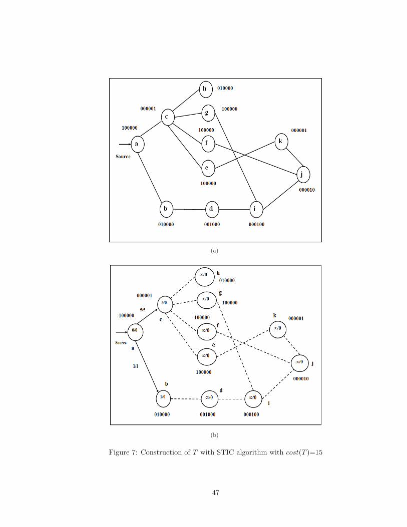
(a)
(b)
Figure 7: Construction of T with STIC algorithm with cost(T )=15
47
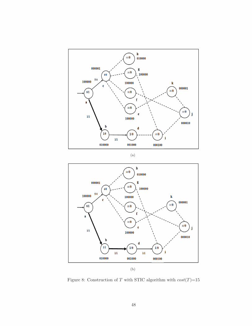
(a)
(b)
Figure 8: Construction of T with STIC algorithm with cost(T )=15
48
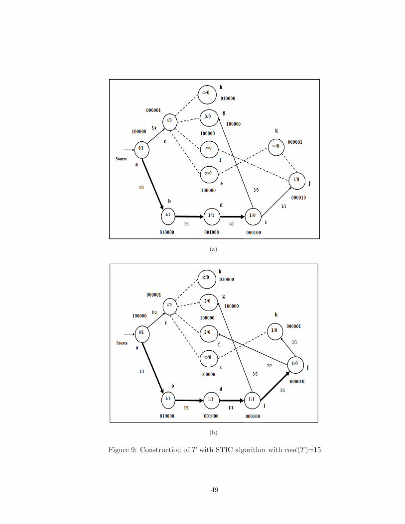
(a)
(b)
Figure 9: Construction of T with STIC algorithm with cost(T )=15
49
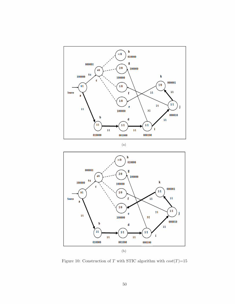
(a)
(b)
Figure 10: Construction of T with STIC algorithm with cost(T )=15
50
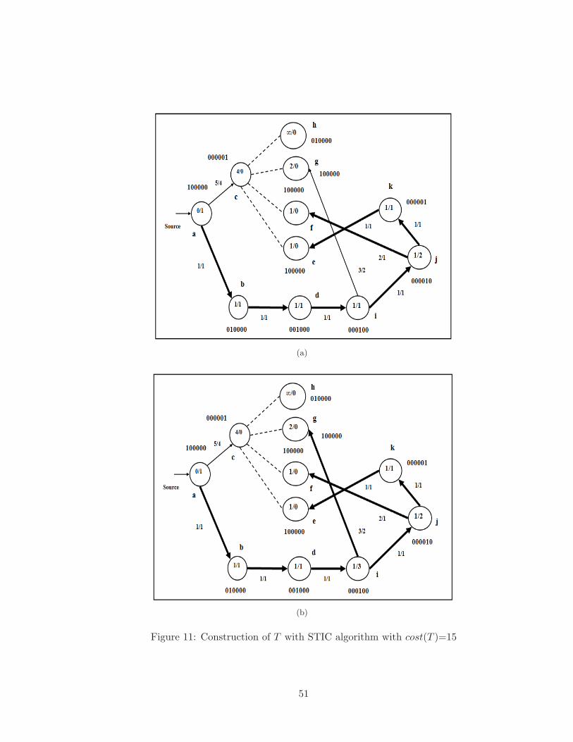
(a)
(b)
Figure 11: Construction of T with STIC algorithm with cost(T )=15
51
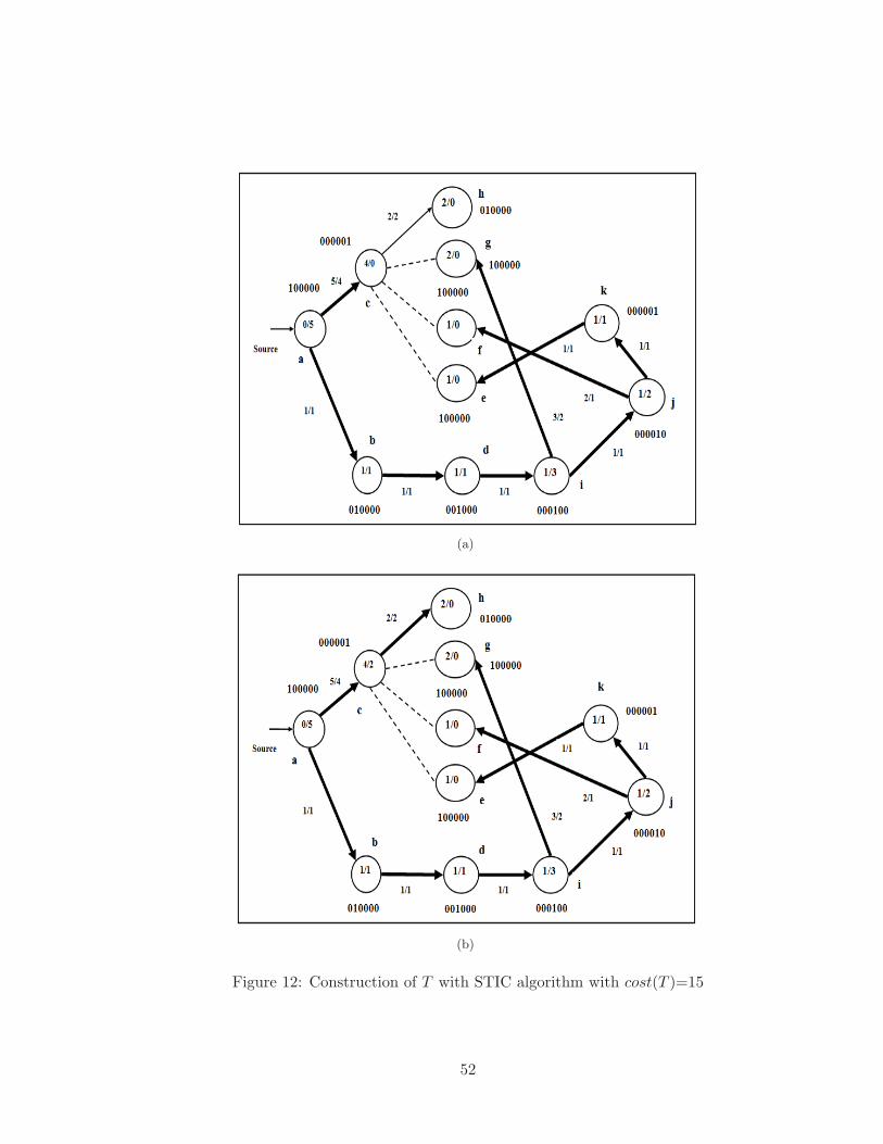
(a)
(b)
Figure 12: Construction of T with STIC algorithm with cost(T )=15
52

3.3.2 MST Edmonds Algorithm
This algorithm is based on Edmonds’ algorithm for finding the minimum cost spanning tree
in a directed graph [10]. We calculate the cost of the edges based on the active time units
of the nodes. We consider the wireless sensor network G = (V,E,M) as a directed graph
and proceed through the following steps:
1. Weight Calculation: As in the STIC algorithm, the cost of an arc (u, v) is calculated
as w(u, v) = t′ − t (mod n), where t and t′ are the active time units of u and v
respectively and the subtraction is done in modulo n arithmetic.
2. Initialization: All the incoming arcs into s are discarded and for every node u other
than s, its lowest cost incoming arc is selected as its only incoming arc. This set of
N − 1 arcs is denoted by S.
3. Contraction of Nodes: If S does not contain any cycle, then S is the desired
broadcast tree. Otherwise, for each cycle C, all the nodes involved in C, are replaced
by a pseudo-node p(C) in G and the resulting graph is denoted by G′. Let x(C) be the
cost of the minimum cost arc in C. The weight of each arc which enters a node j in C
from some node i outside C is modified as w(i, p(C)) = w(i, j)−(w(pred(j), j)−x(C)),
where pred(j) is the predecessor of j in C. We recursively call the algorithm on G′.
4. Extraction of Nodes: Given the broadcast tree S′ that is the output of the recursive
call, each pseudo-node v in S′ is replaced by the nodes involved in the original cycle
corresponding to v. The arc (i, v) in the tree S′ corresponds to an arc (i, x) in the
original graph G where x ∈ C. We include the arc (i, x) in S and remove the incoming
arc into x in the cycle C. This ensures that S is a tree.
After constructing broadcast tree T , the broadcast schedule is determined and the cost is
calculated. The complexity of the algorithm is O(mlogN) for sparse graphs and O(N2) for
dense graphs. The pseudocode of the algorithm is shown in Algorithm 2.
53

Algorithm 2 MST Edmonds Algorithm for Broadcast Tree Construction
Input: Duty cycled WSN G = (V,E,M) and source s ∈ VOutput: Broadcast Tree S
procedure Initializationfor all (u, v) ∈ E do
w(u, v) ← t′ − t (mod n)end forDiscard all the incoming arcs into s
end procedure
procedure Contraction Node(G)S ← 0for all u ∈ V and u �= s do
Select (v, u) with lowest w(v, u)pred(u) ← vS ← S ∪ {(v, u)}
end for
if S does not contain any cycle thenreturn S;
elseG′ ← Gfor all Cycles C ∈ S do
x(C) ← Cost of min cost arc in CRemove C and all incident arcs from G′
Replace C with a pseudo-node p(C)cycle(p(C)) ← Cfor all (u, v) ∈ E where u ∈ C and v /∈ C do
Add (p(C), v) to G′
w(p(C), v) ← w(u, v)replace(p(C), v) ← (u, v)
end forfor all (u, v) ∈ E where v ∈ C and u /∈ C do
Add an edge (u, p(C)) to G′
org(u, p(C)) ← (u, v)w(u, p(C)) = w(u, v)− (w(pred(v), v)− x(C))
end forend forS ←Contraction Node(G′)
end ifend procedure
54
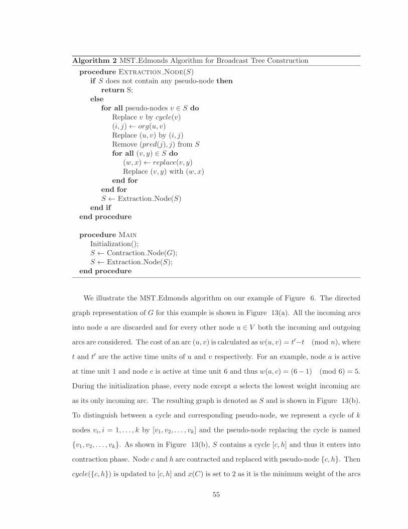
Algorithm 2 MST Edmonds Algorithm for Broadcast Tree Construction
procedure Extraction Node(S)if S does not contain any pseudo-node then
return S;else
for all pseudo-nodes v ∈ S doReplace v by cycle(v)(i, j) ← org(u, v)Replace (u, v) by (i, j)Remove (pred(j), j) from Sfor all (v, y) ∈ S do
(w, x) ← replace(v, y)Replace (v, y) with (w, x)
end forend forS ← Extraction Node(S)
end ifend procedure
procedure MainInitialization();S ← Contraction Node(G);S ← Extraction Node(S);
end procedure
We illustrate the MST Edmonds algorithm on our example of Figure 6. The directed
graph representation of G for this example is shown in Figure 13(a). All the incoming arcs
into node a are discarded and for every other node u ∈ V both the incoming and outgoing
arcs are considered. The cost of an arc (u, v) is calculated as w(u, v) = t′−t (mod n), where
t and t′ are the active time units of u and v respectively. For an example, node a is active
at time unit 1 and node c is active at time unit 6 and thus w(a, c) = (6− 1) (mod 6) = 5.
During the initialization phase, every node except a selects the lowest weight incoming arc
as its only incoming arc. The resulting graph is denoted as S and is shown in Figure 13(b).
To distinguish between a cycle and corresponding pseudo-node, we represent a cycle of k
nodes vi, i = 1, . . . , k by [v1, v2, . . . , vk] and the pseudo-node replacing the cycle is named
{v1, v2, . . . , vk}. As shown in Figure 13(b), S contains a cycle [c, h] and thus it enters into
contraction phase. Node c and h are contracted and replaced with pseudo-node {c, h}. Thencycle({c, h}) is updated to [c, h] and x(C) is set to 2 as it is the minimum weight of the arcs
55

in [c, h] and org(a, {c, h}) is updated to (a, c) and w(a, {c, h}) becomes 3 as w(a, {c, h}) =w(a, c)−(w(pred(c), c)−x(C)) = 5−(4−2) = 3. Again, org(g, {c, h}) is updated to (g, c) and
w(g, {c, h}) becomes 3 as w(g, {c, h}) = w(g, c)− (w(pred(c), c)− x(C)) = 5− (4− 2) = 3.
Similarly, org(f, {c, h}) is updated to (f, c) and org(e, {c, h}) is updated to (e, c). The
weights w(f, {c, h}) and w(e, {c, h}) are updated to 3. Arc (c, e) ∈ G is replaced with
({c, h}, e) ∈ G′ with w({c, h}, e)=w(c, e)=1. Similarly, (c, f) and (c, g) is replaced with
({c, h}, f) along with w({c, h}, f) = 1 and ({c, h}, g) with w({c, h}, g) = 1, respectively.
Then replace({c, h}, e), replace({c, h}, f) and replace({c, h}, g) are updated to (c, e), (c, f)
and (c, g), respectively. The resulting intermediary graph G′ is shown in Figure 14(a). S′
is obtained from G′ by selecting the lowest cost incoming arc for every node u ∈ V except
a. S′ is shown in Figure 14(b) and as it does not contain any cycle, the algorithm enters
into extraction phase.
In the extraction step, pseudo-node {c, h} is replaced with cycle({c, h}) = [c, h] that is
with node c and h. Arc (a, {c, h}) is replaced with org(a, {c, h}) that is (a, c) with w(a, c) =
5. Then (pred(c), c) that is (h, c) is removed and ({c, h}, e), ({c, h}, f) and ({c, h}, g) are
replaced with replace({c, h}, e) = (c, e), replace({c, h}, f) = (c, f) and replace({c, h}, g) =(c, g), respectively. As resulting S does not contain any cycle, S is the broadcast tree T
with cost(T ) = 11. Broadcast tree T is shown in Figure 15. Active time units for each
node are shown in ().
3.3.3 The Sweep Operation
In this section, we show how to reduce the cost of T constructed by all of the algorithms
using a sweep operation which consists of scanning the nodes and making local adjustments
to the tree. A similar idea was used in [51] to adjust transmission powers of nodes in a
previously constructed solution.
The main idea of our sweep operation is to scan the nodes of T in some pre-specified
order. When a node u is scanned, we check for each node v that can be reached from u
without increasing the active time of u, whether making u the parent of v will decrease
the cost of the tree. To avoid creating a loop, this process excludes the nodes between
56
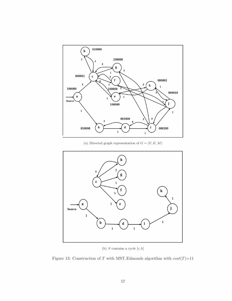
(a) Directed graph representation of G = (V,E,M)
(b) S contains a cycle [c, h]
Figure 13: Construction of T with MST Edmonds algorithm with cost(T )=11
57
(a) Intermediate graph G′ after contracting node c and h
(b) S′ obtained from G′
Figure 14: Construction of T with MST Edmonds algorithm with cost(T )=11
58
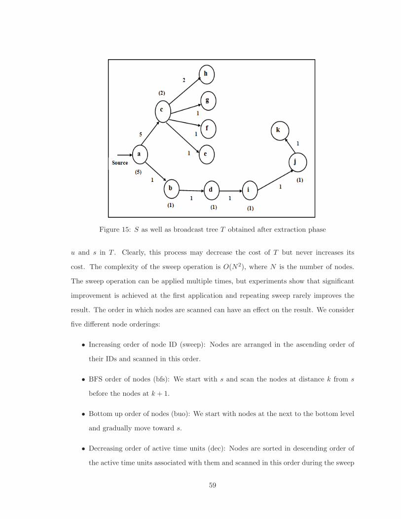
Figure 15: S as well as broadcast tree T obtained after extraction phase
u and s in T . Clearly, this process may decrease the cost of T but never increases its
cost. The complexity of the sweep operation is O(N2), where N is the number of nodes.
The sweep operation can be applied multiple times, but experiments show that significant
improvement is achieved at the first application and repeating sweep rarely improves the
result. The order in which nodes are scanned can have an effect on the result. We consider
five different node orderings:
• Increasing order of node ID (sweep): Nodes are arranged in the ascending order of
their IDs and scanned in this order.
• BFS order of nodes (bfs): We start with s and scan the nodes at distance k from s
before the nodes at k + 1.
• Bottom up order of nodes (buo): We start with nodes at the next to the bottom level
and gradually move toward s.
• Decreasing order of active time units (dec): Nodes are sorted in descending order of
the active time units associated with them and scanned in this order during the sweep
59

operation.
• Increasing order of active time units (inc): Nodes are sorted in ascending order of
active time units associated with them and then scanned accordingly in the sweep
operation.
A sweep operation using any of the above orderings can be performed on the broadcast
tree produced by any algorithm. We denote a broadcast tree algorithm augmented by a
particular type of sweep by Algorithm sweeptype. For example, the MST Edmonds algo-
rithm augmented by a sweep in order of increasing order of active time units (inc) is called
MST Edmonds inc.
We illustrate the sweep operation on T generated by STIC algorithm as shown in Fig-
ure 16(a). Each node u is labeled inside the circle with the additional active time units
for which it is awake. We consider the increasing node ID version of the sweep opera-
tion(STIC sweep) that is, nodes are scanned in increasing order of node ID starting with
node a. Node a and b do not cause any improvement to cost(T ). Node c has to stay awake
2 time units to send messages to node h as it is the only parent of h. During this active
time period, it can also transmit messages to node e, f and g (as shown in Figure 16(a), e,
f and g are shaded to indicate that they are in transmission range of node c). By making c
the parent of e, f and g we can eliminate 1 active time unit from k (the previous parent of
e), 1 time unit from j (the previous parent of f) and 2 time units from i (previous parent
of g). Thus it reduces 4 time units without increasing the number of time units that node
c needs to be active. No other nodes of T cause any improvement of cost(T ). Thus the
sweep operation improves the cost by 4 time units. The cost of the final broadcast tree T
is 11 in this example.
60
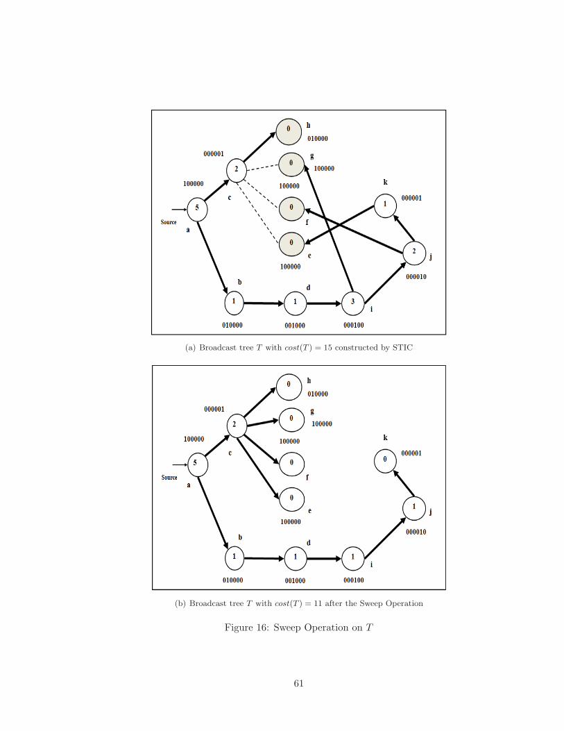
(a) Broadcast tree T with cost(T ) = 15 constructed by STIC
(b) Broadcast tree T with cost(T ) = 11 after the Sweep Operation
Figure 16: Sweep Operation on T
61
Chapter 4
Experimental Results
In this chapter, we present the performance analysis of our proposed algorithms. We con-
ducted extensive simulations in order to compare the performance of the proposed algo-
rithms with two existing algorithms for broadcasting named CSCA [18] and SDT [22]
described in Chapter 2. The main performance metrics used were the average number
of additional active time units per node, the distribution of energy usage over the nodes,
the number of node transmissions and the maximum and average delay of the broadcast
operation.
In all our simulations, we used Java Platform (JDK 6 update 14). We generated networks
where the nodes were distributed uniformly at random in a geographic area of 200 by 200.
We considered networks with the number of nodes 50, 100, 150, 200, 250, 300, 350 and 400.
The number of nodes in a network is denoted by N . For each value of N , we generated
1000 connected graphs and they were stored in a file. For each value of N , the same graphs
were used across all simulations. All the results in this chapter are averaged over 1000
topologies. We used the density measures of 8, 10 and 12. Given the node density measure
we calculated the transmission range of a node for each value of N . Two nodes are adjacent
if and only if their Euclidean distance is less than or equal to the transmission range. For
each topology, a source node which is responsible for initiating the broadcast message is
selected at random. Every node in the network is accompanied with a wakeup schedule
which is a binary array of fixed length. We used the schedule length sch len of 5, 10, 15
62
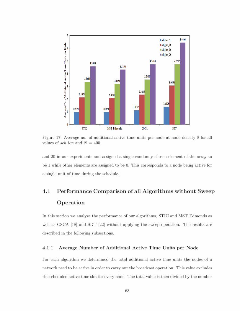
Figure 17: Average no. of additional active time units per node at node density 8 for allvalues of sch len and N = 400
and 20 in our experiments and assigned a single randomly chosen element of the array to
be 1 while other elements are assigned to be 0. This corresponds to a node being active for
a single unit of time during the schedule.
4.1 Performance Comparison of all Algorithms without Sweep
Operation
In this section we analyze the performance of our algorithms, STIC and MST Edmonds as
well as CSCA [18] and SDT [22] without applying the sweep operation. The results are
described in the following subsections.
4.1.1 Average Number of Additional Active Time Units per Node
For each algorithm we determined the total additional active time units the nodes of a
network need to be active in order to carry out the broadcast operation. This value excludes
the scheduled active time slot for every node. The total value is then divided by the number
63
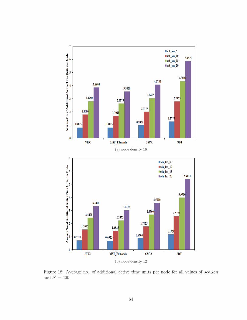
(a) node density 10
(b) node density 12
Figure 18: Average no. of additional active time units per node for all values of sch lenand N = 400
64

Table 1: Average Additional Active Time Units per Node with respect to MST Edmondsfor N=400 and sch len=20
Node Density STIC MST Edmonds CSCA SDT
8 1.06 1.00 1.10 1.49
10 1.09 1.00 1.15 1.65
12 1.10 1.00 1.18 1.78
of nodes in a network to obtain the average number of additional active time units per node.
Both of our proposed algorithms STIC and MST Edmonds reduce the average number of
additional active time units per node as compared to CSCA and SDT, while MST Edmonds
produces a slightly better result. The SDT algorithm shows the worst performance among
all the algorithms. Our results are illustrated in Figures 17 to 18 for N=400. As can be
seen from Figure 17, at node density 8 for sch len=20, the average additional active time
units per node for STIC and MST Edmonds are 4.5800 and 4.3150, respectively which in
turn indicate that on average, a node has to stay awake additional time which is about
23% and 22% of the schedule for the STIC algorithm and for the MST Edmonds algorithm,
respectively. On the other hand, CSCA and SDT cause a node to be alive for about 24% and
32% of the schedule, respectively for the same value of sch len. All the algorithms reduce
the additional active time units per node to a greater extent with the higher values of node
density. For example, as depicted in Figure 18(b), at node density 12 for sch len=20,
the average additional active time units per node for STIC, MST Edmonds, CSCA and
SDT are 3.3400, 3.0325, 3.5900 and 5.4050, respectively. That is at node density 12 a node
needs to be active only about 17% and 15% of the schedule for STIC and MST Edmonds,
respectively. A node has to stay active for about 18% of the schedule for CSCA while SDT
causes a node to be active for about 27% of the schedule. Both CSCA and SDT produce
larger percentage of additional active time units per node compared to MST Edmonds and
STIC and these percentages are gradually increased with higher values of node density.
The normalized results with respect to MST Edmonds for N=400 and sch len=20 are
shown in Table 1. For example, at node density=12, on average, STIC produces about
10% more additional active time units compared to MST Edmonds while CSCA produces
65
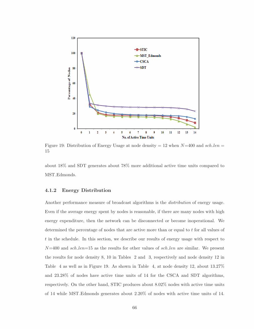
Figure 19: Distribution of Energy Usage at node density = 12 when N=400 and sch len =15
about 18% and SDT generates about 78% more additional active time units compared to
MST Edmonds.
4.1.2 Energy Distribution
Another performance measure of broadcast algorithms is the distribution of energy usage.
Even if the average energy spent by nodes is reasonable, if there are many nodes with high
energy expenditure, then the network can be disconnected or become inoperational. We
determined the percentage of nodes that are active more than or equal to t for all values of
t in the schedule. In this section, we describe our results of energy usage with respect to
N=400 and sch len=15 as the results for other values of sch len are similar. We present
the results for node density 8, 10 in Tables 2 and 3, respectively and node density 12 in
Table 4 as well as in Figure 19. As shown in Table 4, at node density 12, about 13.27%
and 23.28% of nodes have active time units of 14 for the CSCA and SDT algorithms,
respectively. On the other hand, STIC produces about 8.02% nodes with active time units
of 14 while MST Edmonds generates about 2.20% of nodes with active time units of 14.
66
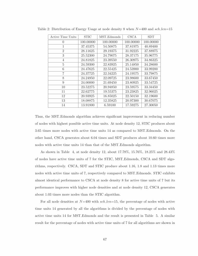
Table 2: Distribution of Energy Usage at node density 8 when N=400 and sch len=15
Active Time Units STIC MST Edmonds CSCA SDT
0 100.00000 100.00000 100.00000 100.00000
1 37.45375 54.50875 37.81975 40.89400
2 28.11625 29.19375 31.92225 37.88975
3 25.52300 24.79075 28.37175 35.96775
4 24.81825 23.39550 26.30975 34.86325
5 24.59300 22.83925 25.14850 34.28600
6 24.47625 22.55425 24.53900 33.99200
7 24.37725 22.34225 24.19575 33.79875
8 24.24950 22.09725 23.98600 33.67450
9 24.00000 21.69450 23.80925 33.54725
10 23.52275 20.94850 23.59575 33.34450
11 22.62775 19.55375 23.23825 32.96025
12 20.93925 16.85025 22.50150 32.19600
13 18.08875 12.35825 20.97300 30.67075
14 13.91800 6.59100 17.59275 27.30050
Thus, the MST Edmonds algorithm achieves significant improvement in reducing number
of nodes with highest possible active time units. At node density 12, STIC produces about
3.65 times more nodes with active time units 14 as compared to MST Edmonds. On the
other hand, CSCA generates about 6.04 times and SDT produces about 10.60 times more
nodes with active time units 14 than that of the MST Edmonds algorithm.
As shown in Table 4, at node density 12, about 17.78%, 15.76%, 18.25% and 28.43%
of nodes have active time units of 7 for the STIC, MST Edmonds, CSCA and SDT algo-
rithms, respectively. CSCA, SDT and STIC produce about 1.16, 1.8 and 1.13 times more
nodes with active time units of 7, respectively compared to MST Edmonds. STIC exhibits
almost identical performance to CSCA at node density 8 for active time units of 7 but its
performance improves with higher node densities and at node density 12, CSCA generates
about 1.03 times more nodes than the STIC algorithm.
For all node densities at N=400 with sch len=15, the percentage of nodes with active
time units 14 generated by all the algorithms is divided by the percentage of nodes with
active time units 14 for MST Edmonds and the result is presented in Table 5. A similar
result for the percentage of nodes with active time units of 7 for all algorithms are shown in
67

Table 3: Distribution of Energy Usage at node density 10 when N=400 and sch len=15
Active Time Units STIC MST Edmonds CSCA SDT
0 100.00000 100.00000 100.00000 100.00000
1 34.25550 49.65250 32.92550 36.96125
2 24.09050 23.90775 27.71600 34.43300
3 21.43850 20.36300 24.58850 32.85200
4 20.84225 19.33750 22.72950 31.91725
5 20.66725 18.90950 21.67150 31.41850
6 20.57775 18.67575 21.08975 31.13300
7 20.48750 18.49650 20.76725 30.97550
8 20.35225 18.26925 20.57025 30.86700
9 20.09375 17.86750 20.41300 30.75500
10 19.58650 17.11825 20.22425 30.58350
11 18.64175 15.69600 19.90550 30.23900
12 16.89850 12.99275 19.26050 29.56425
13 14.11125 8.68975 17.93850 28.17675
14 10.45925 3.82150 15.03250 25.17275
Table 4: Distribution of Energy Usage at node density 12 when N=400 and sch len=15
Active Time Units STIC MST Edmonds CSCA SDT
0 100.00000 100.00000 100.00000 100.00000
1 32.11250 45.54600 29.22275 33.57350
2 21.30500 20.15525 24.64050 31.41275
3 18.64075 17.27875 21.87325 30.06450
4 18.07650 16.45000 20.13850 29.25350
5 17.92975 16.11175 19.12450 28.79700
6 17.86925 15.92300 18.56825 28.57275
7 17.77875 15.76350 18.25325 28.43300
8 17.63875 15.54050 18.06525 28.33825
9 17.35225 15.13675 17.92775 28.23750
10 16.83075 14.37850 17.77125 28.08600
11 15.87100 12.95975 17.49675 27.81300
12 14.07800 10.26050 16.96275 27.19850
13 11.34825 6.18925 15.81425 25.96175
14 8.02375 2.19675 13.27450 23.28275
68
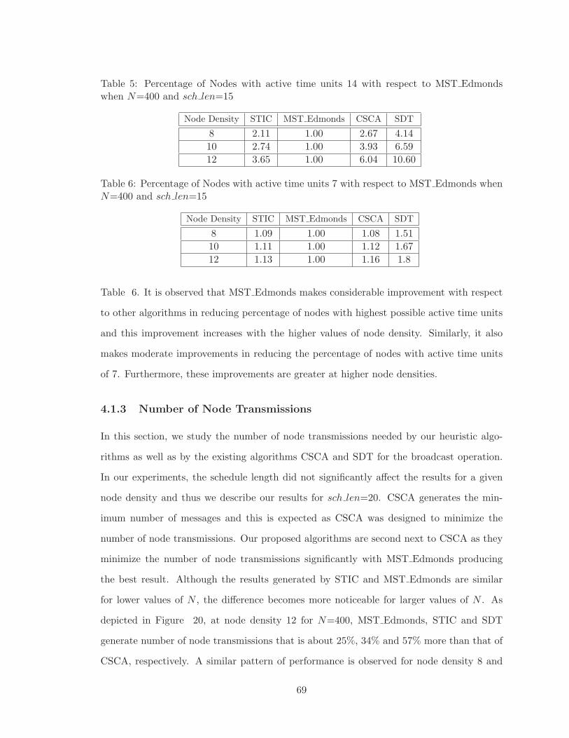
Table 5: Percentage of Nodes with active time units 14 with respect to MST Edmondswhen N=400 and sch len=15
Node Density STIC MST Edmonds CSCA SDT
8 2.11 1.00 2.67 4.14
10 2.74 1.00 3.93 6.59
12 3.65 1.00 6.04 10.60
Table 6: Percentage of Nodes with active time units 7 with respect to MST Edmonds whenN=400 and sch len=15
Node Density STIC MST Edmonds CSCA SDT
8 1.09 1.00 1.08 1.51
10 1.11 1.00 1.12 1.67
12 1.13 1.00 1.16 1.8
Table 6. It is observed that MST Edmonds makes considerable improvement with respect
to other algorithms in reducing percentage of nodes with highest possible active time units
and this improvement increases with the higher values of node density. Similarly, it also
makes moderate improvements in reducing the percentage of nodes with active time units
of 7. Furthermore, these improvements are greater at higher node densities.
4.1.3 Number of Node Transmissions
In this section, we study the number of node transmissions needed by our heuristic algo-
rithms as well as by the existing algorithms CSCA and SDT for the broadcast operation.
In our experiments, the schedule length did not significantly affect the results for a given
node density and thus we describe our results for sch len=20. CSCA generates the min-
imum number of messages and this is expected as CSCA was designed to minimize the
number of node transmissions. Our proposed algorithms are second next to CSCA as they
minimize the number of node transmissions significantly with MST Edmonds producing
the best result. Although the results generated by STIC and MST Edmonds are similar
for lower values of N , the difference becomes more noticeable for larger values of N . As
depicted in Figure 20, at node density 12 for N=400, MST Edmonds, STIC and SDT
generate number of node transmissions that is about 25%, 34% and 57% more than that of
CSCA, respectively. A similar pattern of performance is observed for node density 8 and
69
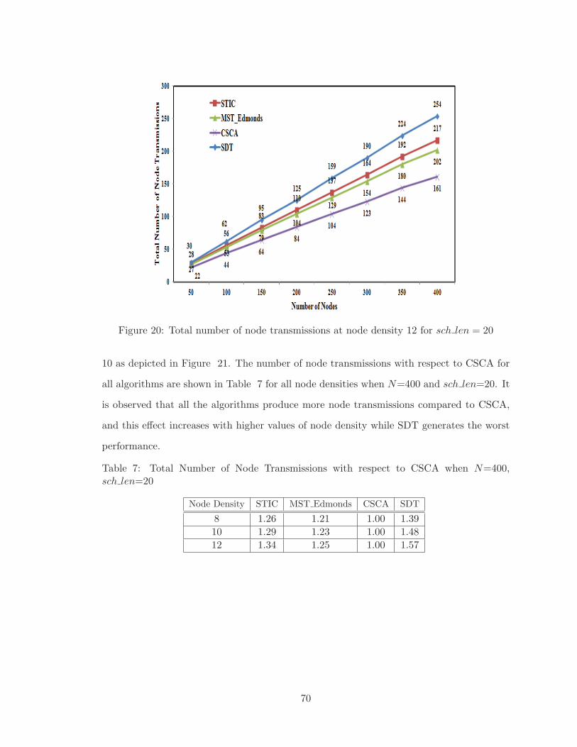
Figure 20: Total number of node transmissions at node density 12 for sch len = 20
10 as depicted in Figure 21. The number of node transmissions with respect to CSCA for
all algorithms are shown in Table 7 for all node densities when N=400 and sch len=20. It
is observed that all the algorithms produce more node transmissions compared to CSCA,
and this effect increases with higher values of node density while SDT generates the worst
performance.
Table 7: Total Number of Node Transmissions with respect to CSCA when N=400,sch len=20
Node Density STIC MST Edmonds CSCA SDT
8 1.26 1.21 1.00 1.39
10 1.29 1.23 1.00 1.48
12 1.34 1.25 1.00 1.57
70
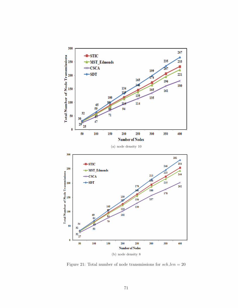
(a) node density 10
(b) node density 8
Figure 21: Total number of node transmissions for sch len = 20
71

Figure 22: Maximum Delay of the Network at node density 12 for sch len = 20
4.1.4 Maximum Delay of Broadcast Operation
We describe our results for maximum delay with respect to sch len 20. At all node densities,
SDT generates the smallest value of maximum delay among all the algorithms. The STIC
algorithm exhibits the closest performance to it. As depicted in Figure 22, at node density
12 for N=400, STIC produces maximum delay which is about 36.05% larger than that of
SDT whereas MST Edmonds and CSCA generate delay which is about 125.45% and 128%
larger than that of the same algorithm, respectively. MST Edmonds performs in a similar
way to CSCA at node density 12 for higher values of N as shown in Figure 22 but for lower
densities, it has worse performance than CSCA for larger values of N. The results for node
density 10 and 8 are shown in Figures 23(a) and 23(b), respectively. For all node densities,
the maximum delay generated by all the algorithms with respect to SDT are shown in Table
8. It is observed that maximum delay reduces slightly for STIC with higher values of node
density while for CSCA, it gradually increases with increasing node densities compared to
SDT.
72
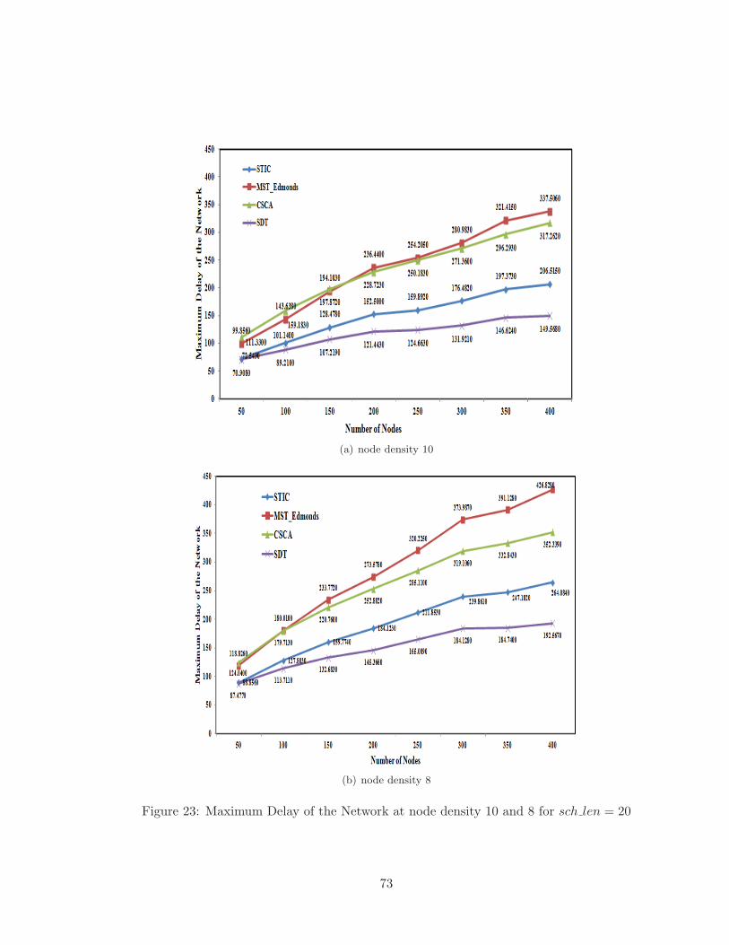
(a) node density 10
(b) node density 8
Figure 23: Maximum Delay of the Network at node density 10 and 8 for sch len = 20
73

Table 8: Normalized Maximum Delay with respect to SDT when N=400 and sch len=20
Node Density STIC MST Edmonds CSCA SDT
8 1.37 2.22 1.83 1.00
10 1.38 2.26 2.12 1.00
12 1.36 2.25 2.28 1.00
4.1.5 Average Delay of Broadcast Operation
SDT generates the minimum average delay for broadcast operation at all node densities.
Figures 24, 25(a) and 25(b), illustrate the result for node density 12, 10 and 8, respectively.
STIC always generates the result closest to SDT and particularly atN=50, it produces lower
delay than the SDT at all node densities. As depicted in Figure 24, at node density 12
for N=400, it produces about 22% more delay as compared to that of the SDT algorithm
while MST Edmonds generates about 116% more delay than the same algorithm. CSCA
generates about 126% more delay than the SDT algorithm at the same node density for
N=400. MST Edmonds and CSCA generate about 77% and 85% more delay respectively
compared to STIC at node density 12. MST Edmonds exhibits the worst performance at
node density 8 although it produces better result than CSCA upto N=150. Its performance
improves with increasing node densities as and finally at node density 12, MST Edmonds
generates better result than CSCA for all values of N .
Table 9: Normalized Average Delay with respect to SDT when N=400 and sch len=20
Node Density STIC MST Edmonds CSCA SDT
8 1.28 2.15 1.81 1.00
10 1.26 2.16 2.09 1.00
12 1.22 2.16 2.26 1.00
For all node densities, the average delay of all the algorithms with respect to SDT is
shown in Table 9 for N=400 and sch len=20. It is observed that with higher values of
node density the performance of STIC improves while the performance of CSCA degrades
compared to the SDT algorithm.
74
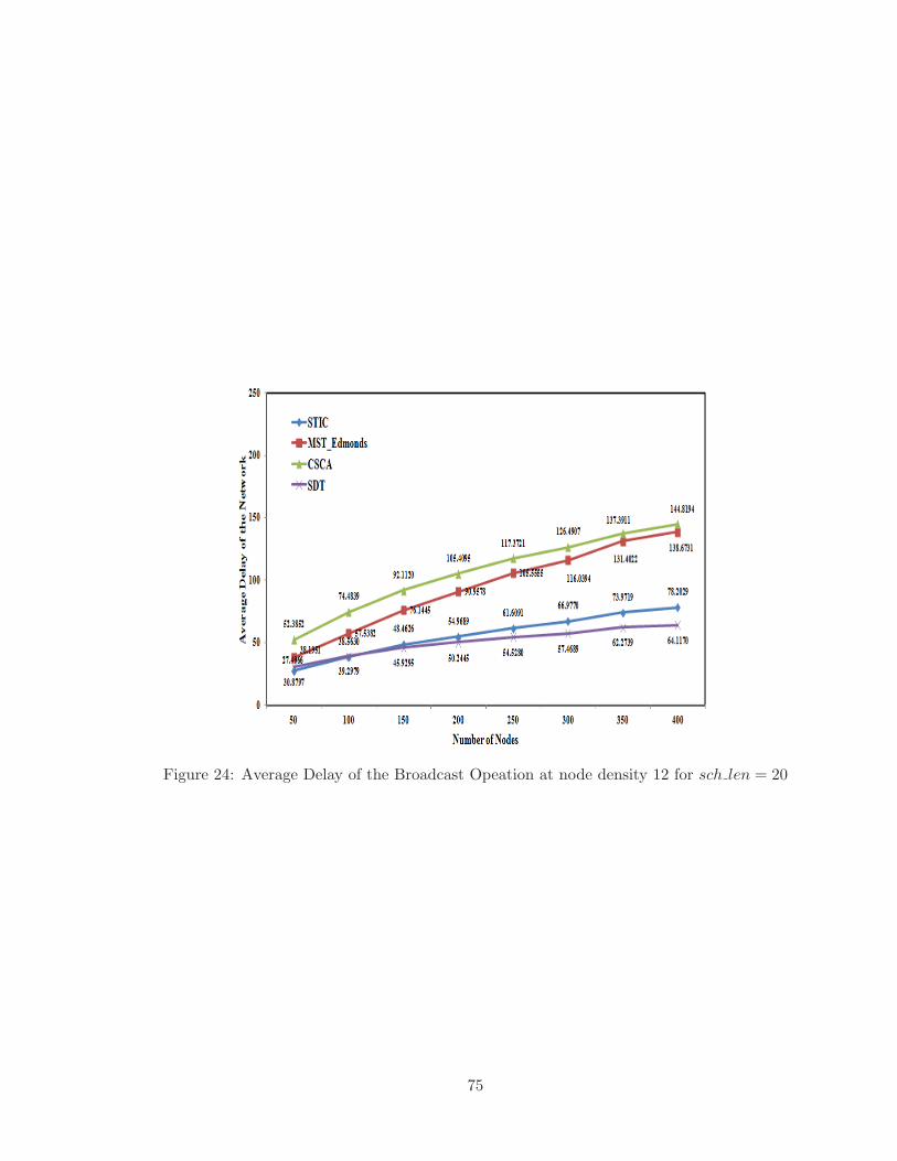
Figure 24: Average Delay of the Broadcast Opeation at node density 12 for sch len = 20
75
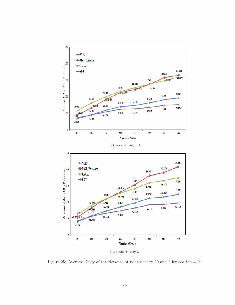
(a) node density 10
(b) node density 8
Figure 25: Average Delay of the Network at node density 10 and 8 for sch len = 20
76
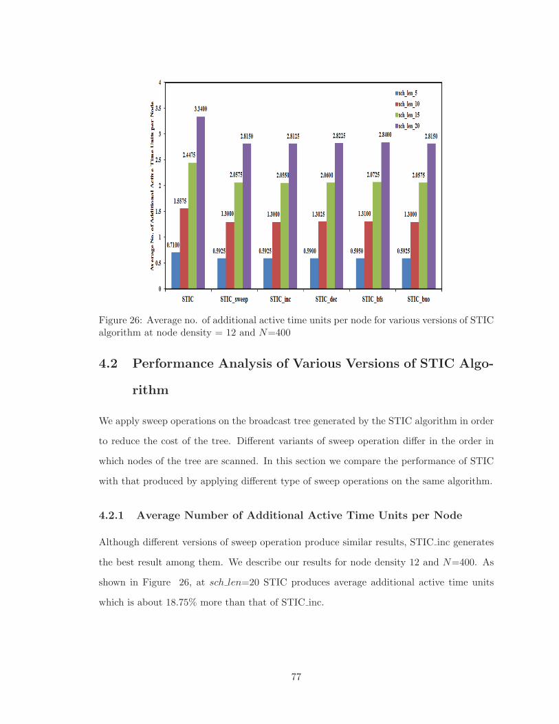
Figure 26: Average no. of additional active time units per node for various versions of STICalgorithm at node density = 12 and N=400
4.2 Performance Analysis of Various Versions of STIC Algo-
rithm
We apply sweep operations on the broadcast tree generated by the STIC algorithm in order
to reduce the cost of the tree. Different variants of sweep operation differ in the order in
which nodes of the tree are scanned. In this section we compare the performance of STIC
with that produced by applying different type of sweep operations on the same algorithm.
4.2.1 Average Number of Additional Active Time Units per Node
Although different versions of sweep operation produce similar results, STIC inc generates
the best result among them. We describe our results for node density 12 and N=400. As
shown in Figure 26, at sch len=20 STIC produces average additional active time units
which is about 18.75% more than that of STIC inc.
77

Figure 27: Distribution of Energy Usage for STIC and STIC inc algorithms at node density= 12 for N=400 and sch len=15
4.2.2 Energy Distribution
We compare the energy usage of STIC with STIC inc as it gives the best result among
all variants of sweep operation. We describe the result for node density 12 , N=400 and
sch len=15. As shown in Figure 27, at node density 12, about 8.02% nodes have active
time units of 14 for STIC while about 6.343% of nodes have active time units of 14 for
STIC inc. Thus, given a schedule length STIC inc is more capable of reducing the number
of nodes with highest possible active time units. At node density 12, STIC generates about
1.26 times more nodes having active time units of 14 while it produces about 1.18 times
more nodes with active time units of 7 compared to STIC inc.
4.2.3 Number of Node Transmissions
STIC inc gives the best result in terms of number of node transmissions and we analyze the
result of STIC and STIC inc for sch len=20 at node density 12. As shown in Figure 28,
at node density=12 for N=400, STIC generates about 17.30% more node transmissions as
78
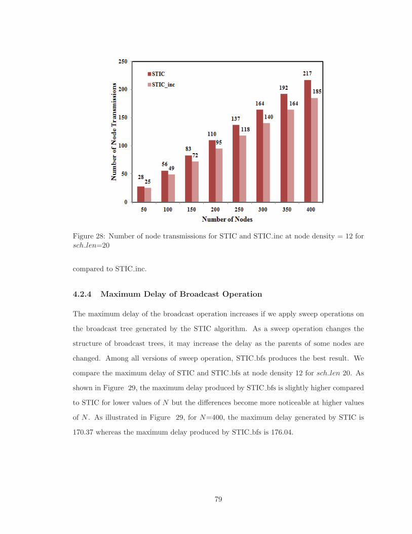
Figure 28: Number of node transmissions for STIC and STIC inc at node density = 12 forsch len=20
compared to STIC inc.
4.2.4 Maximum Delay of Broadcast Operation
The maximum delay of the broadcast operation increases if we apply sweep operations on
the broadcast tree generated by the STIC algorithm. As a sweep operation changes the
structure of broadcast trees, it may increase the delay as the parents of some nodes are
changed. Among all versions of sweep operation, STIC bfs produces the best result. We
compare the maximum delay of STIC and STIC bfs at node density 12 for sch len 20. As
shown in Figure 29, the maximum delay produced by STIC bfs is slightly higher compared
to STIC for lower values of N but the differences become more noticeable at higher values
of N . As illustrated in Figure 29, for N=400, the maximum delay generated by STIC is
170.37 whereas the maximum delay produced by STIC bfs is 176.04.
79
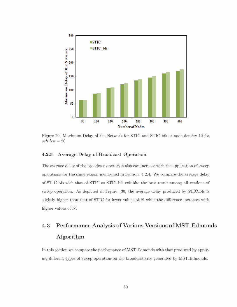
Figure 29: Maximum Delay of the Network for STIC and STIC bfs at node density 12 forsch len = 20
4.2.5 Average Delay of Broadcast Operation
The average delay of the broadcast operation also can increase with the application of sweep
operations for the same reason mentioned in Section 4.2.4. We compare the average delay
of STIC bfs with that of STIC as STIC bfs exhibits the best result among all versions of
sweep operation. As depicted in Figure 30, the average delay produced by STIC bfs is
slightly higher than that of STIC for lower values of N while the difference increases with
higher values of N .
4.3 Performance Analysis of Various Versions of MST Edmonds
Algorithm
In this section we compare the performance of MST Edmonds with that produced by apply-
ing different types of sweep operation on the broadcast tree generated by MST Edmonds.
80

Figure 30: Average Delay of the Network for STIC and STIC bfs at node density 12 forsch len = 20
4.3.1 Average Number of Additional Active Time Units per Node
MST Edmonds bfs produces the best result among various versions of the sweep operation.
As illustrated in Figure 31, at node density=12 for N=400 and sch len=20, MST Edmonds
produces about 16.86% more average additional active time units per node compared to
MST Edmonds bfs.
4.3.2 Energy Distribution
We compare the energy usage of MST Edmonds with MST Edmonds bfs as it gives the best
result among all sweep variants. As shown in Figure 32, at node density 12 for N=400 and
sch len=15, about 2.20% and 1.64% of nodes have active time units of 14 for MST Edmonds
and MST Edmonds bfs, respectively. About 13.67% of nodes have active time units of 7
for MST Edmonds bfs while 15.76% nodes have active time units of 7 for MST Edmonds.
Thus at node density 12, MST Edmonds generates about 1.34 times more nodes with active
time units of 14 while it produces about 1.15 times more nodes with active time units of 7
81
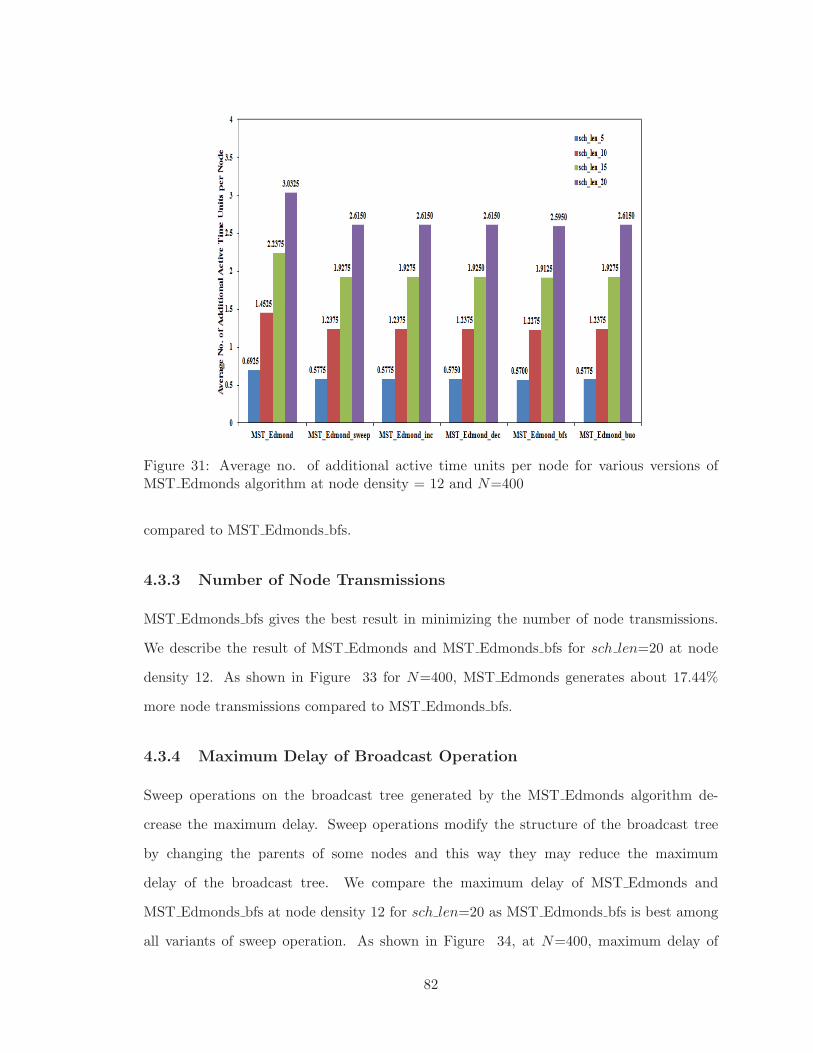
Figure 31: Average no. of additional active time units per node for various versions ofMST Edmonds algorithm at node density = 12 and N=400
compared to MST Edmonds bfs.
4.3.3 Number of Node Transmissions
MST Edmonds bfs gives the best result in minimizing the number of node transmissions.
We describe the result of MST Edmonds and MST Edmonds bfs for sch len=20 at node
density 12. As shown in Figure 33 for N=400, MST Edmonds generates about 17.44%
more node transmissions compared to MST Edmonds bfs.
4.3.4 Maximum Delay of Broadcast Operation
Sweep operations on the broadcast tree generated by the MST Edmonds algorithm de-
crease the maximum delay. Sweep operations modify the structure of the broadcast tree
by changing the parents of some nodes and this way they may reduce the maximum
delay of the broadcast tree. We compare the maximum delay of MST Edmonds and
MST Edmonds bfs at node density 12 for sch len=20 as MST Edmonds bfs is best among
all variants of sweep operation. As shown in Figure 34, at N=400, maximum delay of
82

Figure 32: Distribution of Energy Usage for MST Edmonds and MST Edmonds bfs algo-rithms at node density = 12 for N=400 and sch len=15
Figure 33: Number of node transmissions for MST Edmonds and MST Edmonds bfs atnode density = 12 for sch len=20
83
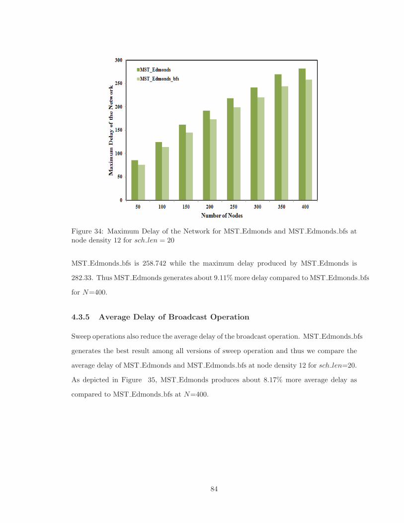
Figure 34: Maximum Delay of the Network for MST Edmonds and MST Edmonds bfs atnode density 12 for sch len = 20
MST Edmonds bfs is 258.742 while the maximum delay produced by MST Edmonds is
282.33. Thus MST Edmonds generates about 9.11% more delay compared to MST Edmonds bfs
for N=400.
4.3.5 Average Delay of Broadcast Operation
Sweep operations also reduce the average delay of the broadcast operation. MST Edmonds bfs
generates the best result among all versions of sweep operation and thus we compare the
average delay of MST Edmonds and MST Edmonds bfs at node density 12 for sch len=20.
As depicted in Figure 35, MST Edmonds produces about 8.17% more average delay as
compared to MST Edmonds bfs at N=400.
84
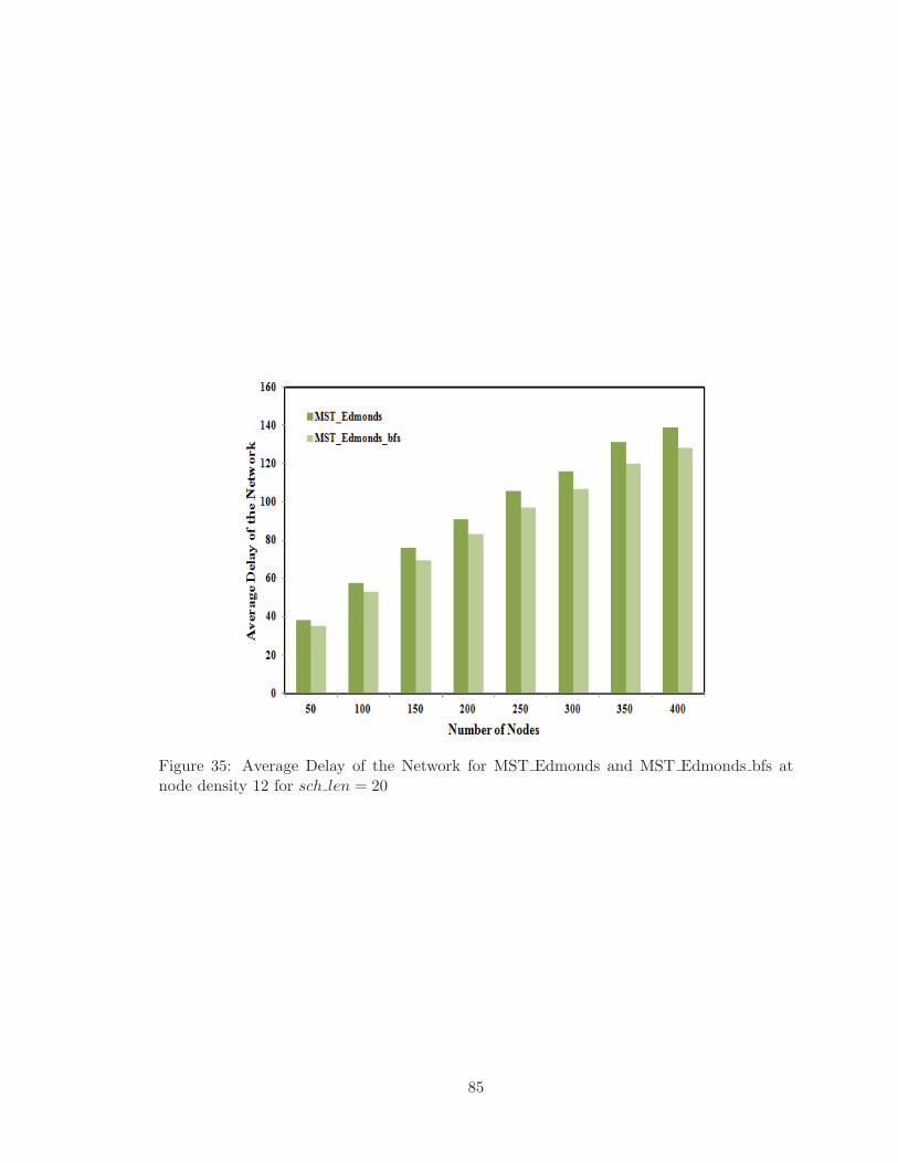
Figure 35: Average Delay of the Network for MST Edmonds and MST Edmonds bfs atnode density 12 for sch len = 20
85

Table 10: Improvements obtained by the sweep operation at node density 12 for N=400:metric for best variant of sweep divided by metric for algorithm without sweep
Cost Measure STIC MST Edmonds CSCA SDT
Additional active time units 0.84 0.86 0.84 0.69per node for sch len = 20
Percentage of nodes with active 0.79 0.75 0.81 0.61time units 14 for sch len = 15
Number of Node Transmissions 0.85 0.85 0.93 0.83for sch len=20
Maximum Delay for sch len=20 1.03 0.92 0.96 1.16
Average Delay for sch len=20 1.04 0.92 0.96 1.11
4.4 Summary of Effect of Sweep Operation
As shown in Table 10, all variants of sweep operation generally reduce all the cost measures
for all our algorithms. The only exceptions are the maximum and average delay for STIC
and SDT. However, the sweep variant that gives the best result for different combinations of
cost measure and broadcast tree algorithm is not always the same. The best sweep variant
for different combinations is presented in Table 11. In the remaining sections, we always
use the best sweep variant of the algorithm when comparing with other algorithms.
Table 11: Best version of sweep operation for various combinations of broadcast tree algo-rithm and cost measure
cost measure MST Edmonds STIC CSCA SDT
Additional active time bfs inc bfs incunits per node
Energy Usage of Nodes bfs inc bfs inc
Number of Node Transmissions bfs inc bfs inc
Maximum Delay bfs no sweep bfs no sweep
Average Delay bfs no sweep bfs no sweep
4.5 Performance Comparison of all Algorithms with Sweep
Operations
In this section, we compare the performance of STIC, MST Edmonds, CSCA [18] and
SDT [22] after applying the sweep operations on the broadcast tree generated by these
86

Table 12: Average Additional Active Time Units per Node for N=400 and sch len = 20
Node Density STIC inc MST Edmonds bfs CSCA bfs SDT inc
8 3.8800 3.6275 4.1150 4.6075
10 3.2550 3.0150 3.4650 4.0850
12 2.8125 2.5950 3.0025 3.7325
Table 13: Average Additional Active Time Units per Node with respect toMST Edmonds bfs for N=400 and sch len = 20
Node Density STIC inc MST Edmonds bfs CSCA bfs SDT inc
8 1.07 1.00 1.13 1.27
10 1.08 1.00 1.15 1.35
12 1.08 1.00 1.16 1.44
algorithms.
4.5.1 Average Number of Additional Active Time Units per Node
For all node densities, we describe our results with respect to N=400 and sch len = 20.
The results are given in Tables 12 and 13. Both STIC inc and MST Edmonds bfs utilize
a smaller number of additional active time units per node as compared to CSCA bfs and
SDT inc, while MST Edmonds bfs produces slightly better result than the STIC inc algo-
rithm. For all node densities and schedule lengths, SDT inc exhibits the worst performance
among all the algorithms. With higher values of node density all algorithms utilize fewer
additional active time units per node, which is to be expected.
As depicted in Table 12, at node density 12 for sch len = 20, the average additional
active time units for MST Edmonds bfs and STIC inc are 2.5950 and 2.8125, respectively.
Thus, on average, a node has to stay awake for additional time which about 13% and 14% of
the schedule to participate in the broadcast operation for MST Edmonds bfs and STIC inc,
respectively. CSCA bfs causes a node to remain alive for about 15% of the schedule and
SDT inc causes a node to be active for about 19% of the schedule for the same value of
sch len. At node density 12, STIC inc, CSCA bfs and SDT inc produce about 8.4%, 16%
and 44% more additional active time units per node compared to MST Edmonds bfs. At
the same node density, CSCA bfs and SDT inc generate about 6.76% and 32.7% more
87
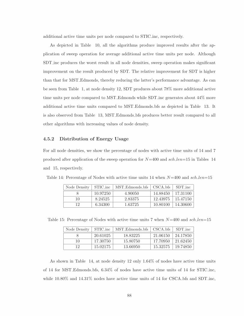
additional active time units per node compared to STIC inc, respectively.
As depicted in Table 10, all the algorithms produce improved results after the ap-
plication of sweep operation for average additional active time units per node. Although
SDT inc produces the worst result in all node densities, sweep operation makes significant
improvement on the result produced by SDT. The relative improvement for SDT is higher
than that for MST Edmonds, thereby reducing the latter’s performance advantage. As can
be seen from Table 1, at node density 12, SDT produces about 78% more additional active
time units per node compared to MST Edmonds while SDT inc generates about 44% more
additional active time units compared to MST Edmonds bfs as depicted in Table 13. It
is also observed from Table 13, MST Edmonds bfs produces better result compared to all
other algorithms with increasing values of node density.
4.5.2 Distribution of Energy Usage
For all node densities, we show the percentage of nodes with active time units of 14 and 7
produced after application of the sweep operation for N=400 and sch len=15 in Tables 14
and 15, respectively.
Table 14: Percentage of Nodes with active time units 14 when N=400 and sch len=15
Node Density STIC inc MST Edmonds bfs CSCA bfs SDT inc
8 10.97250 4.90050 14.88450 17.31100
10 8.24525 2.83375 12.43975 15.47150
12 6.34300 1.63725 10.80100 14.30600
Table 15: Percentage of Nodes with active time units 7 when N=400 and sch len=15
Node Density STIC inc MST Edmonds bfs CSCA bfs SDT inc
8 20.61025 18.83225 21.06150 24.17850
10 17.30750 15.80750 17.70950 21.62450
12 15.02175 13.66950 15.32575 19.74850
As shown in Table 14, at node density 12 only 1.64% of nodes have active time units
of 14 for MST Edmonds bfs, 6.34% of nodes have active time units of 14 for STIC inc,
while 10.80% and 14.31% nodes have active time units of 14 for CSCA bfs and SDT inc,
88

respectively. Thus MST Edmonds bfs significantly reduces the number of nodes with high-
est possible active time units. STIC inc generates about 3.87 times more nodes with active
time units of 14 than the MST Edmonds bfs algorithm. CSCA bfs and SDT inc produce
about 6.59 and 8.74 times more such nodes, respectively compared to MST Edmonds bfs.
Also as shown in Table 15, at node density 12, only 13.67% nodes have active time
units of 7 for MST Edmonds bfs while 15.02%, 15.33% and 19.75% nodes have active time
units of 7 for STIC inc, CSCA bfs and SDT inc, respectively. This in turn indicates that
STIC inc, CSCA bfs and SDT inc produce about 1.10, 1.12 and 1.44 times more such nodes,
respectively compared to MST Edmonds bfs. Thus, MST Edmonds bfs not only constructs
a tree with the lowest average number of additional active time units per node, it also
appears to create fewer highly loaded nodes and thus increasing the network lifetime. For
all node densities, the percentage of nodes with active time units 14 and 7 for all algorithms
with respect to MST Edmonds bfs are shown in Tables 16 and 17, respectively.
Table 16: Percentage of Nodes with active time units of 14 with respect toMST Edmonds bfs when N=400 and sch len=15
Node Density STIC inc MST Edmonds bfs CSCA bfs SDT inc
8 2.24 1.00 3.04 3.53
10 2.91 1.00 4.39 5.46
12 3.87 1.00 6.60 8.74
Table 17: Percentage of Nodes with active time units of 7 with respect to MST Edmonds bfswhen N=400 and sch len=15
Node Density STIC inc MST Edmonds bfs CSCA bfs SDT inc
8 1.09 1.00 1.12 1.28
10 1.09 1.00 1.12 1.37
12 1.10 1.00 1.12 1.44
As can be seen from Table 16 and 17, MST Edmonds bfs exhibits better perfor-
mance with higher values of node density compared to all other algorithms. SDT inc
produces worst performance in all node densities but its performance gap with respect to
MST Edmonds bfs reduces more compared to that of the SDT with respect to MST Edmonds.
As shown in Table 5, at node density 12, SDT has 10.60 times the number of nodes with
89
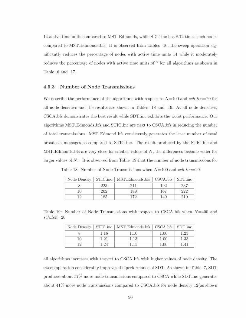
14 active time units compared to MST Edmonds, while SDT inc has 8.74 times such nodes
compared to MST Edmonds bfs. It is observed from Tables 10, the sweep operation sig-
nificantly reduces the percentage of nodes with active time units 14 while it moderately
reduces the percentage of nodes with active time units of 7 for all algorithms as shown in
Table 6 and 17.
4.5.3 Number of Node Transmissions
We describe the performance of the algorithms with respect to N=400 and sch len=20 for
all node densities and the results are shown in Tables 18 and 19. At all node densities,
CSCA bfs demonstrates the best result while SDT inc exhibits the worst performance. Our
algorithms MST Edmonds bfs and STIC inc are next to CSCA bfs in reducing the number
of total transmissions. MST Edmond bfs consistently generates the least number of total
broadcast messages as compared to STIC inc. The result produced by the STIC inc and
MST Edmonds bfs are very close for smaller values of N , the differences become wider for
larger values of N . It is observed from Table 19 that the number of node transmissions for
Table 18: Number of Node Transmissions when N=400 and sch len=20
Node Density STIC inc MST Edmonds bfs CSCA bfs SDT inc
8 223 211 192 237
10 202 189 167 222
12 185 172 149 210
Table 19: Number of Node Transmissions with respect to CSCA bfs when N=400 andsch len=20
Node Density STIC inc MST Edmonds bfs CSCA bfs SDT inc
8 1.16 1.10 1.00 1.23
10 1.21 1.13 1.00 1.33
12 1.24 1.15 1.00 1.41
all algorithms increases with respect to CSCA bfs with higher values of node density. The
sweep operation considerably improves the performance of SDT. As shown in Table 7, SDT
produces about 57% more node transmissions compared to CSCA while SDT inc generates
about 41% more node transmissions compared to CSCA bfs for node density 12(as shown
90
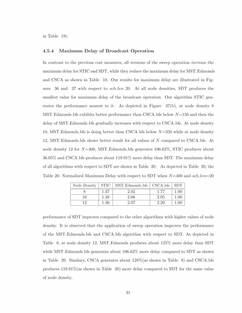
in Table 19).
4.5.4 Maximum Delay of Broadcast Operation
In contrast to the previous cost measures, all versions of the sweep operation increase the
maximum delay for STIC and SDT, while they reduce the maximum delay for MST Edmonds
and CSCA as shown in Table 10. Our results for maximum delay are illustrated in Fig-
ures 36 and 37 with respect to sch len 20. At all node densities, SDT produces the
smallest value for maximum delay of the broadcast operation. Our algorithm STIC gen-
erates the performance nearest to it. As depicted in Figure 37(b), at node density 8
MST Edmonds bfs exhibits better performance than CSCA bfs below N=150 and then the
delay of MST Edmonds bfs gradually increases with respect to CSCA bfs. At node density
10, MST Edmonds bfs is doing better than CSCA bfs below N=350 while at node density
12, MST Edmonds bfs shows better result for all values of N compared to CSCA bfs. At
node density 12 for N=400, MST Edmonds bfs generates 106.62%, STIC produces about
36.05% and CSCA bfs produces about 119.91% more delay than SDT. The maximum delay
of all algorithms with respect to SDT are shown in Table 20. As depicted in Table 20, the
Table 20: Normalized Maximum Delay with respect to SDT when N=400 and sch len=20
Node Density STIC MST Edmonds bfs CSCA bfs SDT
8 1.37 2.02 1.77 1.00
10 1.38 2.06 2.05 1.00
12 1.36 2.07 2.20 1.00
performance of SDT improves compared to the other algorithms with higher values of node
density. It is observed that the application of sweep operation improves the performance
of the MST Edmonds bfs and CSCA bfs algorithm with respect to SDT. As depicted in
Table 8, at node density 12, MST Edmonds produces about 125% more delay than SDT
while MST Edmonds bfs generates about 106.62% more delay compared to SDT as shown
in Table 20. Similary, CSCA generates about 128%(as shown in Table 8) and CSCA bfs
produces 119.91%(as shown in Table 20) more delay compared to SDT for the same value
of node density.
91
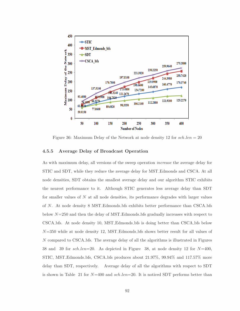
Figure 36: Maximum Delay of the Network at node density 12 for sch len = 20
4.5.5 Average Delay of Broadcast Operation
As with maximum delay, all versions of the sweep operation increase the average delay for
STIC and SDT, while they reduce the average delay for MST Edmonds and CSCA. At all
node densities, SDT obtains the smallest average delay and our algorithm STIC exhibits
the nearest performance to it. Although STIC generates less average delay than SDT
for smaller values of N at all node densities, its performance degrades with larger values
of N . At node density 8 MST Edmonds bfs exhibits better performance than CSCA bfs
below N=250 and then the delay of MST Edmonds bfs gradually increases with respect to
CSCA bfs. At node density 10, MST Edmonds bfs is doing better than CSCA bfs below
N=350 while at node density 12, MST Edmonds bfs shows better result for all values of
N compared to CSCA bfs. The average delay of all the algorithms is illustrated in Figures
38 and 39 for sch len=20. As depicted in Figure 38, at node density 12 for N=400,
STIC, MST Edmonds bfs, CSCA bfs produces about 21.97%, 99.94% and 117.57% more
delay than SDT, respectively. Average delay of all the algorithms with respect to SDT
is shown in Table 21 for N=400 and sch len=20. It is noticed SDT performs better than
92
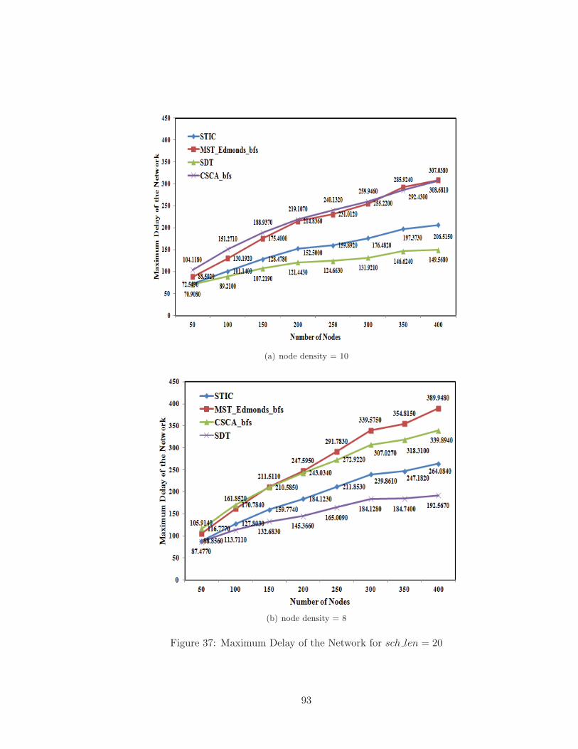
(a) node density = 10
(b) node density = 8
Figure 37: Maximum Delay of the Network for sch len = 20
93

Figure 38: Average Delay of the Network at node density 12 for sch len = 20
Table 21: Normalized Average Delay with respect to SDT when N=400, sch len=20
Node Density STIC MST Edmonds bfs CSCA bfs SDT
8 1.28 1.97 1.74 1.00
10 1.26 1.99 2.02 1.00
12 1.22 1.99 2.18 1.00
other algorithms with increasing values of node density. The sweep operation considerably
improves the performance of MST Edmonds and CSCA compared to SDT. As shown in
Table 9, at node density 12 MST Edmonds produces about 116% more delay compared
to SDT while MST Edmonds bfs generates about 99.94% more delay compared to the
same algorithm for N=400 as depicted in Table 21. Similarly, CSCA generates about
126%(as shown in Table 9) more delay compared to SDT while CSCA bfs generates about
117.57%(as shown in Table 21) more delay compared to the same algorithm at the same
node density for N=400.
94
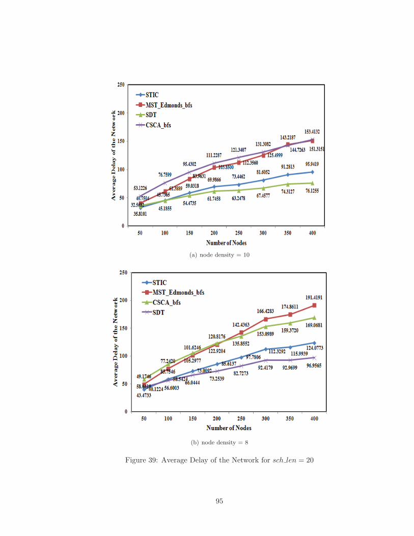
(a) node density = 10
(b) node density = 8
Figure 39: Average Delay of the Network for sch len = 20
95
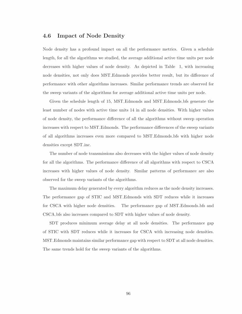
4.6 Impact of Node Density
Node density has a profound impact on all the performance metrics. Given a schedule
length, for all the algorithms we studied, the average additional active time units per node
decreases with higher values of node density. As depicted in Table 1, with increasing
node densities, not only does MST Edmonds provides better result, but its difference of
performance with other algorithms increases. Similar performance trends are observed for
the sweep variants of the algorithms for average additional active time units per node.
Given the schedule length of 15, MST Edmonds and MST Edmonds bfs generate the
least number of nodes with active time units 14 in all node densities. With higher values
of node density, the performance difference of all the algorithms without sweep operation
increases with respect to MST Edmonds. The performance differences of the sweep variants
of all algorithms increases even more compared to MST Edmonds bfs with higher node
densities except SDT inc.
The number of node transmissions also decreases with the higher values of node density
for all the algorithms. The performance difference of all algorithms with respect to CSCA
increases with higher values of node density. Similar patterns of performance are also
observed for the sweep variants of the algorithms.
The maximum delay generated by every algorithm reduces as the node density increases.
The performance gap of STIC and MST Edmonds with SDT reduces while it increases
for CSCA with higher node densities. The performance gap of MST Edmonds bfs and
CSCA bfs also increases compared to SDT with higher values of node density.
SDT produces minimum average delay at all node densities. The performance gap
of STIC with SDT reduces while it increases for CSCA with increasing node densities.
MST Edmonds maintains similar performance gap with respect to SDT at all node densities.
The same trends hold for the sweep variants of the algorithms.
96
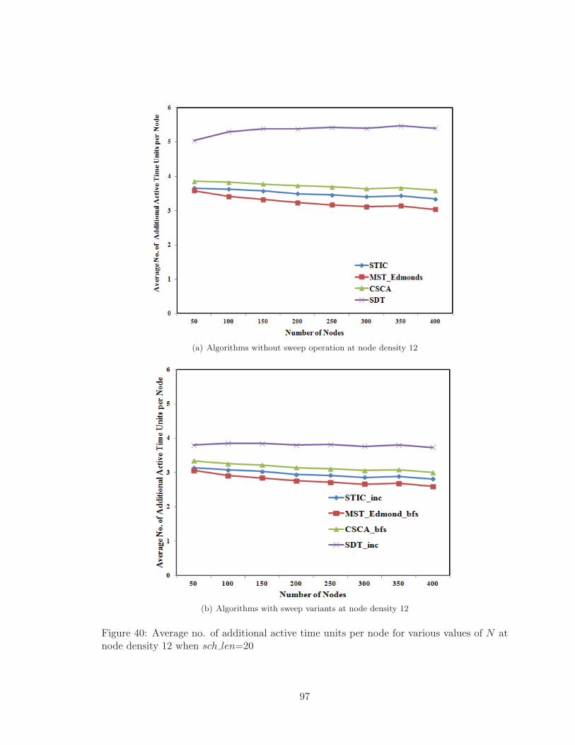
(a) Algorithms without sweep operation at node density 12
(b) Algorithms with sweep variants at node density 12
Figure 40: Average no. of additional active time units per node for various values of N atnode density 12 when sch len=20
97
4.7 Impact of Number of Nodes
At every node density, the impact of the number of nodes on additional active time units
per node, energy distribution and average node transmissions is small. The average addi-
tional active time units for each node decreases slightly with larger values of N for STIC,
MST Edmonds and CSCA at node density 12. As shown in Figure 40(a), SDT starts with
a smaller value at N=50, then this value increases at N=100 after which the value remains
the same for higher values of N . As depicted in Figure 40(b), similar performance trends
are noticed for STIC inc, MST Edmonds bfs and CSCA bfs. SDT inc maintains almost the
same average additional active time units per node for all values of N .
As shown in Figure 41(a), given the sch len 15, the percentage of nodes with active time
units 14 generated by STIC and MST Edmonds reduces slightly with larger values of N .
CSCA generates similar percentage of nodes with active time units 14 for all values of N .
SDT starts with a smaller value at N=50 and then increases up to N=150 and then main-
tains almost the same value for other values of N . For STIC inc and MST Edmonds bfs,
the percentage of nodes with active time units 14 gradually reduces with higher values of
N depicted in Figure 41(b). For SDT inc and CSCA bfs this percentage slightly decreases
at N=400 compared to that at N=50.
CSCA produces smallest average node transmissions among all the algorithms. As
shown in Figure 42(a), at node density 12, average node transmissions for CSCA slightly
reduces at N=400 compared to that at N=50. MST Edmonds and STIC produce similar
values for all N . SDT starts with a smaller value at N=50 and increases up to N=150.
It slightly drops at N=200 and then maintains almost similar values for remaining N .
As depicted in Figure 42(b), the average number of node transmissions for CSCA bfs,
MST Edmonds bfs and STIC inc slightly reduces with larger values of N . For SDT inc,
average node transmissions starts with a smaller value at N=50 and increases upto N=100
and then maintains similar result for the remaining values of N .
The maximum delay of the broadcast operation increases with larger values of N for all
algorithms. SDT generates the minimum value of the maximum delay in all node densities.
98
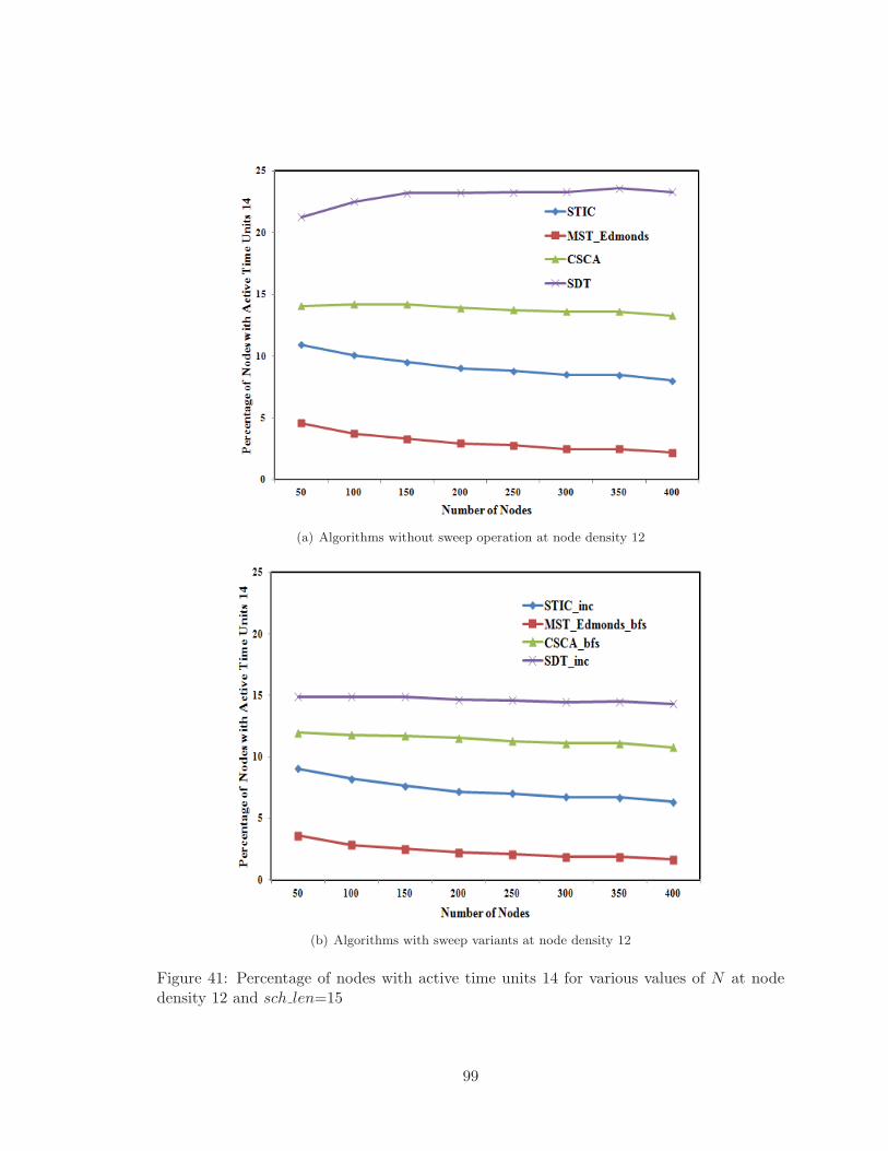
(a) Algorithms without sweep operation at node density 12
(b) Algorithms with sweep variants at node density 12
Figure 41: Percentage of nodes with active time units 14 for various values of N at nodedensity 12 and sch len=15
99
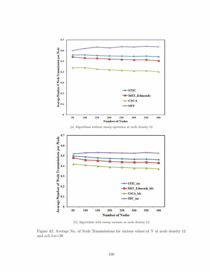
(a) Algorithms without sweep operation at node density 12
(b) Algorithms with sweep variants at node density 12
Figure 42: Average No. of Node Transmissions for various values of N at node density 12and sch len=20
100
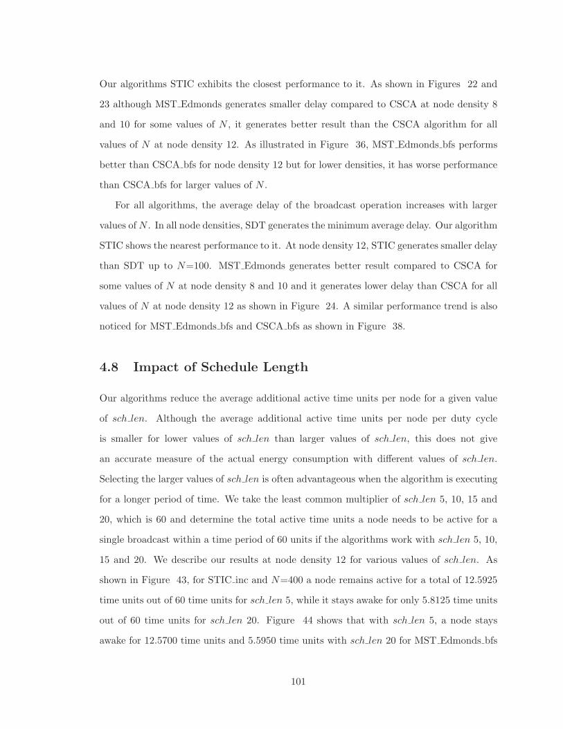
Our algorithms STIC exhibits the closest performance to it. As shown in Figures 22 and
23 although MST Edmonds generates smaller delay compared to CSCA at node density 8
and 10 for some values of N , it generates better result than the CSCA algorithm for all
values of N at node density 12. As illustrated in Figure 36, MST Edmonds bfs performs
better than CSCA bfs for node density 12 but for lower densities, it has worse performance
than CSCA bfs for larger values of N .
For all algorithms, the average delay of the broadcast operation increases with larger
values ofN . In all node densities, SDT generates the minimum average delay. Our algorithm
STIC shows the nearest performance to it. At node density 12, STIC generates smaller delay
than SDT up to N=100. MST Edmonds generates better result compared to CSCA for
some values of N at node density 8 and 10 and it generates lower delay than CSCA for all
values of N at node density 12 as shown in Figure 24. A similar performance trend is also
noticed for MST Edmonds bfs and CSCA bfs as shown in Figure 38.
4.8 Impact of Schedule Length
Our algorithms reduce the average additional active time units per node for a given value
of sch len. Although the average additional active time units per node per duty cycle
is smaller for lower values of sch len than larger values of sch len, this does not give
an accurate measure of the actual energy consumption with different values of sch len.
Selecting the larger values of sch len is often advantageous when the algorithm is executing
for a longer period of time. We take the least common multiplier of sch len 5, 10, 15 and
20, which is 60 and determine the total active time units a node needs to be active for a
single broadcast within a time period of 60 units if the algorithms work with sch len 5, 10,
15 and 20. We describe our results at node density 12 for various values of sch len. As
shown in Figure 43, for STIC inc and N=400 a node remains active for a total of 12.5925
time units out of 60 time units for sch len 5, while it stays awake for only 5.8125 time units
out of 60 time units for sch len 20. Figure 44 shows that with sch len 5, a node stays
awake for 12.5700 time units and 5.5950 time units with sch len 20 for MST Edmonds bfs
101

Figure 43: Total Active Time Units per Node for STIC inc in a time period of 60 at nodedensity=12
for the same value of N . Clearly it is much more energy-efficient to work with a longer
schedule length, if broadcast operations happen infrequently and if a smaller duty cycle is
not dictated by other reasons.
102
Figure 44: Total Active Time Units per Node for MST Edmonds bfs in a time period of 60at node density=12
103
Chapter 5
Conclusions and Future Work
In this thesis, we discussed the significance of providing energy efficient broadcast mecha-
nism for duty cycled WSNs in order to ensure the longer network lifetime. The broadcast
operation is essential for executing many network activities like routing, topology control,
data acquisition, etc. We formulated the problem of constructing an energy efficient broad-
cast tree for duty cycled WSNs as the MEBT problem and proved that it is NP-hard. We
proposed two polynomial time algorithms MST Edmonds and STIC for constructing an
energy-efficient broadcast tree in a duty cycled WSN and then applied several variants of
a sweep operation that perform local adjustments on a broadcast tree in order to improve
its cost. Simulation results show that our algorithms outperform other previous algorithms
in terms of total number of additional active time units and produce the lowest number
of highly loaded nodes, with MST Edmonds being the best of all algorithms. At the same
time, they have good performance in terms of maximum and average delay as well as num-
ber of node transmissions. MST Edmonds is better than STIC in terms of the minimum
number of transmissions, while the latter algorithm has better delay performance.
The broadcast operation in duty cycled WSNs is highly challenging due to the ac-
tive/sleep nature of the sensor nodes. Moreover, the problem gets compounded by the
unreliable nature of the communication links. We are interested to find broadcast solutions
for duty cycled WSNs that will address the unreliable communication links along with a
104
mechanism to handle the collisions in order to reduce the number of redundant retrans-
missions. We proposed two polynomial time heuristic algorithms for the MEBT problem.
In future we are interested in finding efficient algorithms with provable performance ratios.
Finding a solution for delay efficient broadcasting in duty cycled WSNs is an appealing
problem. Adapting the existing broadcast mechanisms of always operational networks for
the duty cycled WSNs is also an interesting future research direction. We proposed a
centralized solution to construct energy efficient broadcast trees. We can utilize the knowl-
edge of 2-hop neighborhood information of a node to construct distributed and localized
algorithms. In this thesis, we construct a broadcast tree with respect to a specific node.
However, the construction of a global tree which can be used for broadcast from every
node and has acceptable performance is also an attractive problem. Broadcast algorithms
that will minimize the maximum energy consumption of every node is also another exciting
problem.
105

Bibliography
[1] C. Adjih, P. Jacquet, and L. Viennot. Computing connected dominated sets with
multipoint relays. Ad Hoc and Sensor Networks, 1(1–2):27–39, 2005.
[2] I. F. Akyildiz, W. Su, Y. Sankarasubramaniam, and E. Cayirci. A survey on sensor
networks. IEEE Communications Magazine, 40(8):102–114, 2002.
[3] I. F. Akyildiz, W. Su, Y. Sankarasubramaniam, and E.Cayirci. Wireless sensor net-
works: A survey. Computer Networks, 38(2002):393–422, 2002.
[4] J. N. Al-karaki and A. E. Kamal. Routing techniques in wireless sensor networks: A
survey. IEEE Wireless Communications, 11(6):6–28, 2004.
[5] N. Aydin, M. Karaca, and O. Ercetin. Energy-optimal scheduling in low duty cycle
sensor networks. In SPECTS, 2011: Proceedings of the International Symposium on
Performance Evaluation of Computer and TeleCommunication Systems, pages 119–
126, 2011.
[6] J. Cartigny, F. Ingelrest, D. Simplot-Ryl, and I. Stojmenovic. Localized lmst and rng
based minimum-energy broadcast protocols in ad hoc networks. Ad Hoc Networks,
3(1):1–16, 2005.
[7] J. Cartigny, D. Simplot, and I. Stojmenovic. Localized minimum-energy broadcasting
in ad-hoc networks. In IEEEINFOCOM2003: Proceedings of the 22nd Annual Joint
Conference of the IEEE Computer and Communications Societies, pages 2210–2217,
2003.
106
[8] X. Chen, M. Faloutsos, and S. V. Krishnamurthy. Power adaptive broadcasting with
local information in ad hoc networks. In ICNP2003: Proceedings of the 11th IEEE
International Conference on Network Protocols, pages 168–178, 2003.
[9] C.-F. Chiasserini and M. Garetto. Modeling the performance of wireless sensor net-
works. In INFOCOM’04: Proceedings of the 23rd Conference of the IEEE Communi-
cations Society, pages 220–231, 2004.
[10] J. Edmonds. Optimum branchings. Journal of Research of the National Bureau of
Standards, 71B:233–240, 1967.
[11] Y. Gu and T. He. Data forwarding in extremely low duty-cycle sensor networks with
unreliable communication links. In SenSys’07: Proceedings of the 5th International
Conference on Embedded Networked Sensor Systems, pages 321–334, 2007.
[12] S. Guo, Y. Gu, B. Jiang, and T. He. Opportunistic flooding in low-duty cycle wireless
sensor networks with unreliable link. InMOBICOM’09: Proceedings of the 15th Annual
International Conference on Mobile Computing and Networking, pages 133–144, 2009.
[13] Z. J. Haas, J. Y. Halpern, and L. Li. Gossip-based ad hoc routing. In INFOCOM’02:
Proceedings of Twenty-First Annual Joint Conference of IEEE Computer and Com-
munications Societies, pages 1707–1716, 2002.
[14] Z. J. Haas and M. Nikolov. Towards optimal broadcast in wireless networks. In
MSWIM’11: Proceedings of the 14th ACM International Conference on Modeling,
Analysis and Simulation of Wireless and Mobile Systems, pages 213–222, 2011.
[15] W. Heinzelman, A. Chandrakasan, and H. Balakrishnan. Energy-efficient communi-
cation protocol for wireless microsensor networks. In Proceedings of the 33rd Hawaii
International Conference on System Sciences - 2000, pages 1–10, 2000.
[16] W. Heinzelman, J. Kulik, and H. Balakrishnan. Adaptive protocols for information
dissemination in wireless sensor networks. In MOBICOM,1999: Proceedings of the
107

5th annual ACM/IEEE international conference on Mobile computing and networking,
pages 174–185, 1999.
[17] J. Hong, J. Cao, W. Li, S. Lu, and D. Chen. Sleeping schedule-aware minimum la-
tency broadcast in wireless ad hoc networks. In ICC, 2009: Proceedings of the IEEE
International Conference on Communications, pages 1–5, 2009.
[18] J. Hong, J. Cao, W. Li, S. Lu, and D. Chen. Minimum-transmission broadcast in
uncoordinated duty-cycled wireless ad hoc networks. IEEE Transaction on Vehicular
technology, 59(1):307–318, 2010.
[19] F. Ingelrest and D. Simplot-Ryl. Localized broadcast incremental power protocol for
wireless ad hoc networks. In ISCC2005: Proceedings of the IEEE Symposium on Com-
puters and Communication, pages 28–33, 2005.
[20] F. Ingelrest, D. Simplot-Ryl, and I. Stojmenovic. Optimal transmission radius for en-
ergy efficient broadcasting protocols in ad hoc and sensor networks. IEEE Transactions
on Parallel and Distributed Systems, 17(6):536–547, 2006.
[21] C. Intanagonwiwat, R. Govindan, and D. Estrin. Directed diffusion: a scalable and
robust communication paradigm for sensor networks. In MOBICOM,2000: Proceedings
of the 6th annual international conference on Mobile computing and networking, pages
56–67, 2000.
[22] X. Jiao, W. Lou, J. Ma, J. Cao, X. Wang, and X. Zhou. Minimum latency broadcast
scheduling in duty-cycled multihop wireless networks. IEEE Transactions on Parallel
and Distributed Systems, 23(1):110–117, 2012.
[23] R. Jurdak, A. G. Ruzzelli, and G.M.P. OHare. Radio sleep mode optimization in
wireless sensor networks. IEEE Transactions on Mobile Computing, 9(7):955–968, 2010.
[24] A. Keshavarzian, H. Lee, and L. Venkatraman. Wakeup scheduling in wireless sensor
networks. In MOBIHOC,2006: Proceedings of the 7th ACM international symposium
on Mobile ad hoc networking and computing, pages 322–333, 2006.
108
[25] P. Kysdsnur, R.R. Choudhury, and I. Gupta. Smart gossip: An adaptive gossip-
based broadcasting service for sensor networks. In Proceedings of IEEE International
Conference on Mobile Ad Hoc and Sensor Systems, pages 91–100, 2006.
[26] P. Levis, N. Patel, D. Culler, and S. Shenker. Trickle: A self-regulating algorithm
for code propagation and maintenance in wireless sensor networks. In NSDI’04: Pro-
ceedings of the First USENIX/ACM Symposium on Networked Systems Design and
Implementation, pages 15–28, 2004.
[27] N. Li and J. C. Hou. BLMST: A scalable, power-efficient broadcast algorithm for
wireless networks. In QSHINE2004: Proceedings of the 1st International Conference
on Quality of Service in Heterogeneous Wired/Wireless Networks, 2004.
[28] W. Liang. Constructing minimum-energy broadcast trees in wireless ad hoc networks.
In MOBIHOC’02: Proceedings of the Third ACM International Symposium on Mobile
Ad Hoc Networking and Computing, pages 112–122, 2002.
[29] H. Lim and C. Kim. Multicast tree construction and flooding in wireless ad hoc
networks. In Proceedings of ACM International Workshop Modeling, Analysis and
Simulation of Wireless and Mobile Systems, pages 61–68, 2000.
[30] W. Lou and J. Wu. On reducing broadcast redundancy in ad hoc wireless networks.
IEEE Transactions on Mobile Computing, 1(2):111–122, 2002.
[31] G. Lu, N. Sadagopan, B. Krishnamachari, and A. Goel. Delay efficient sleep scheduling
in wireless sensor networks. In INFOCOM’05: Proceedings of the 24th Joint Conference
of the IEEE Computer and Communications Societies, pages 2470–2481, 2005.
[32] S.-Y. Ni, Y.-C.Tseng, Y.-S. Chen, and J.-P. Sheu. The broadcast storm problem in a
mobile ad hoc network. In MOBICOM’99:Proceedings of International Conference on
Mobile Computing and Networks, pages 151–162, 1999.
[33] J. Park and S. Sahani. Maximum lifetime broadcasting in wireless networks. IEEE
Transactions on Computers, 54(9):1081–1089, 2005.
109
[34] W. Peng and X-C. Lu. On the reduction of broadcast redundancy in mobile ad hoc
networks. In MOBIHOC,2000: Proceedings of the 1st Annual Workshop on Mobile and
Ad Hoc Networking and Computing, pages 129–130, 2000.
[35] R. C. Prim. Shortest connection networks and some generalizations. Bell System
Technical Journal, 36:1389–1401, 1957.
[36] A. Qayyum, L. Viennot, and A. Laouiti. Multipoint relaying for flooding broadcast
messages in mobile wireless networks. In HICSS-35’02: Proceedings of the 35th Hawaii
International Conference on System Sciences, pages 298–307, 2002.
[37] A. Qayyum, L. Viennot, and A. Laouiti. An enhanced approach to determine a small
forward node set based on multipoint relays. In IEEEVTCH2003: Proceedings of the
of IEEE Vehicular Technology Conferenece, pages 2774–2777, 2003.
[38] A. G. Ruzzelli, P. Cotan, G. M. P. OHare, R. Tynan, and P. J. M havinga. Protocol
assessment issues in low duty cycle sensor networks: The switching energy. In SUTC’06:
Proceedings of IEEE International Conference on Sensor Networks, Ubiquitous and
Trustworthy Computing, pages 101–108, 2006.
[39] K. Selvakumar and S. Nithya. d2-coloring of a graph. The Journal of Mathematics and
Computer Science, 3(2):102–111, 2011.
[40] F. Stann, J. Heidemann, R. Shroff, and M. Z. Murtaza. RBP: Robust broadcast
propagaion in wireless networks. In SenSys2006: Proceedings of the 4th International
Conference on Embedded Networked Sensor Systems, pages 58–98, 2006.
[41] I. Stojmenovic. Comments and corrections to dominating sets and neighbor
elimination-based broadcasting algorithms in wireless networks. IEEE Transactions
on Parallel and Distributed Systems, 15(11):1054–1055, 2004.
[42] I. Stojmenovic, M. Seddigh, and J. Zunic. Dominating sets and neighbor elimination
based broadcasting algorithms in wireless networks. IEEE Transactions on Parallel
and Distributed Systems, 13(1):14–25, 2002.
110
[43] Y. Sun, O. Gurewitz, S. Du, L. Tang, and D. B. Johnson. ADB: An efficient multihop
broadcast protocol based on asynchronous duty-cycling in wireless sensor networks. In
SenSys’09: Proceedings of the 7th ACM Conference on Embedded Networked Sensor
Systems, pages 43–56, 2009.
[44] Y. C. Tseng, S. Y. Ni, and E. Y. Shih. Adaptive approaches for relieving broadcast
storms in wireless multihop mobile ad hoc networks. IEEE Transactions on Computers,
52(5):545–557, 2003.
[45] F. Wang and J. Liu. RBS: A reliable broadcast service for large-scale low duty-cycled
wireless sensor networks. In ICC’08: Proceedings of IEEE International Conference on
Communications, pages 2416–2420, 2008.
[46] F. Wang and J. Liu. Duty-cycle-aware broadcast in wireless sensor networks. In
INFOCOM’09: Proceedings of the 28th Conference on Computer Communications,
pages 468–476, 2009.
[47] W. Wang and B. Soong. Collision-free and low-latency scheduling algorithm for broad-
cast operation in wireless ad hoc networks. IEEE Communications Letters, 11(10):1–3,
2007.
[48] P. Wei and L. Xicheng. AHBP: An efficient broadcast protocol for mobile ad hoc
networks. Journal of Computer Science and Technology, 16(2):114–125, 2001.
[49] J. Wieselthier, G. Nguyen, and A. Ephremides. On the construction of energy-efficient
broadcast and multicast trees in wireless sensor networks. In IEEE INFOCOM 2000:
Proceedings of the 19th Annual Joint Conference of the IEEE Computer and Commu-
nications Societies, pages 585–594, 2000.
[50] J. E. Wieselthier, G. D. Nguyen, and A. Ephremides. Distributed algorithms for energy-
efficient broadcasting in ad hoc networks. In MILCOM,2002: Proceedings of the Mili-
tary Communications Conference, pages 820–825, 2002.
111
[51] J. E. Wieselthier, G. D. Nguyen, and A. Ephremides. Energy-efficient broadcast and
multicast trees for wireless networks. Mobile Networks and Applications, 7(6):481–492,
2002.
[52] J. Wu and H. Li. On calculating connected dominating set for efficient routing in ad hoc
wireless networks. In DlALM1999: Proceedings of the 3rd International Workshop on
Discrete Algorithms and Methods for Mobile Computing and Communications, pages
7–14, 1999.
[53] J. Wu, W. Lou, and F. Dai. Extended multipoint relays to determine connected dom-
inating sets in manets. IEEE Transactions on Computers, 55(3):334–347, 2006.
112