J Sched (2010) 13: 561–576DOI 10.1007/s10951-010-0181-1

Minimizing total weighted tardiness on a single machinewith release dates and equal-length jobs

J.M. van den Akker · G. Diepen · J.A. Hoogeveen

Published online: 1 May 2010© The Author(s) 2010. This article is published with open access at Springerlink.com

Abstract In this paper we study the problem of schedul-ing n jobs with release dates, due dates, weights, and equalprocessing times on a single machine. The objective is tominimize total weighted tardiness. We formulate the prob-lem as a time-indexed ILP after which we solve the LP-relaxation. We show that for certain special cases (namelywhen either all due dates, all weights, or all release dates areequal, or when all due dates and release dates are equallyordered), the solution for the LP-relaxation is either inte-gral or can be adjusted in polynomial time into an inte-gral one. For the general case we present a branching rulethat performs well. Furthermore we show that the same ap-proach holds for the m identical, parallel machines variantof the problem. Finally we show that with a minor modifica-tion the same approach also holds for the single-machineproblems of minimizing the sum of weighted late jobs(1|rj ,pj = p|∑wjUj ) and the sum of weighted late work(1|rj ,pj = p|∑wjVj ) as well as their respective variantswith m identical, parallel machines. We further show howwe can solve these problems by applying column genera-

Supported by BSIK grant 03018 (BRICKS: Basic Research inInformatics for Creating the Knowledge Society).

J.M. van den Akker · J.A. HoogeveenDepartment of Computer Science, Utrecht University,P.O. Box 80089, 3508 TB Utrecht, The Netherlands

J.M. van den Akkere-mail: marjan@cs.uu.nl

J.A. Hoogeveene-mail: slam@cs.uu.nl

G. Diepen (�)Paragon Decision Technology, Schipholweg 1, 2034 LS Haarlem,The Netherlandse-mail: Guido.Diepen@aimms.com

tion when there is not sufficient memory available to applythe direct ILP-approach.

Keywords Common processing time · Weightedtardiness · Time indexed formulation

1 Introduction

The problem we are looking at is the following: We havea single machine on which we have to schedule a set N ={1,2, . . . , n} of jobs, where n is the number of jobs. For eachjob Jj we have a release date rj before which job Jj is notavailable, a due date dj , and a weight wj . The processingtimes of the jobs are all equal to p. We assume the due dates,the release dates, the weights, and the common processingtime of all jobs to be integral. We are looking for a feasibleschedule, that is, we want to find a set of completion timesCj (j = 1, . . . , n) such that no job starts before its releasedate and no two jobs overlap in their execution. Given thecompletion time Cj of a job Jj , we define the tardiness Tj

of job Jj as:

Tj = max{0,Cj − dj }.Now the objective is to find the feasible schedule that mini-mizes the total weighted tardiness. To the best of our knowl-edge the computational complexity of this problem is stillopen.

For writing down the different problems we make useof the three-field notation scheme introduced by Grahamet al. (1979). In this three-field notation scheme the prob-lem of minimizing total weighted tardiness on a single ma-chine with release dates and equal-length jobs is denoted as1|rj ,pj = p|∑wjTj .

562 J Sched (2010) 13: 561–576

Over the years quite some research has been done onscheduling problems regarding (weighted) tardiness. Lawler(1977) gave a pseudopolynomial algorithm for solving the1 ‖ Tj problem and Du and Leung (1990) gave a proof forthe 1 ‖ Tj problem to be N P -hard in the ordinary sense. Theweighted version of this problem, 1 ‖ wjTj , is known to beN P -hard in the strong sense (Lenstra et al. 1977). Akturkand Ozdemir (2001) gave a new dominance rule for solv-ing the 1|rj |wjTj problem to optimality using branch-and-bound.

Also quite some research has been done on schedulingproblems with equal processing times: Baptiste (2000) looksat the 1|rj ,pj = p|∑Tj problem, as well as the prob-lem with m identical, parallel machines instead of one andshows that both problems can be solved in polynomial timeby means of dynamic programming. Baptiste (1999) givesa polynomial time algorithm for the 1|rj ,pj = p|∑wjUj

problem based on dynamic programming. In Baptiste et al.(2004) ten equal-processing-time scheduling problems areshown to be solvable in polynomial time, among which isthe Pm|rj ,pj = p|∑wjUj problem. An overview of moreproblems with equal processing times can be found in Leung(2004).

Verma and Dessouky (1998) look at common processingtime scheduling with earliness and tardiness penalties. Theyformulate this problem as a time-indexed ILP and show thatwhen certain criteria are met, there exists an integral optimalsolution to the LP-relaxation, which means that there existsa polynomial time solution procedure. In this paper we willfollow their approach, and we will show that if certain cri-teria hold, then the 1|rj ,pj = p|∑wjTj problem can besolved in polynomial time.

The outline for the rest of this paper is as follows: InSect. 2 we give an ILP-formulation of the problem. In Sect. 3we will present an algorithm that can be used to rewrite frac-tional solutions for the single-machine problem that possessa special condition of being non-double nested. In Sect. 4we will discuss the special case of the problem in which thejobs have a common due date, and in Sect. 5 we will discussthe general problem. In Sect. 6 we will apply the same tech-niques on problems with related objective functions for thesingle-machine case, and in Sect. 7 we look at the case withm parallel, identical machines. After that in Sect. 8 we willdiscuss another way of solving the problem, which aims atreducing the amount of memory needed, and in Sect. 9 wewill present some experimental results. Finally in Sect. 10we will draw some conclusions.

2 Problem formulation

Like in Verma and Dessouky (1998), we use a time-indexedformulation to represent the problem as an ILP. We restrict

ourselves to those times that can occur as completion timesin an optimal solution. Because of the equal processingtimes, the processing of a job will always occur in an inter-val with length p. We denote each interval by the end time ofthe interval. The objective function that we consider is totalweighted tardiness, and since this is a regular function, therewill always exists an optimal schedule that is left-aligned,that is, it is not possible to execute any job earlier withoutpostponing any other job.

Since there exists an optimal schedule that is left-aligned,we can restrict ourselves to schedules in which each job, ei-ther starts at its release date, or immediately after anotherjob. Hence, each release date introduces a set of possiblecompletions times, and in the extreme case some job Jj willstart right at its release date after which all other jobs fol-low contiguously. This means that job Jj introduces (n − 1)

possible completion times for the other jobs.Unless another job Jj ′ has a release date that is a mul-

tiple of p before rj , only job Jj can be completed at timeγj = rj + p. We define the set G denoting all first possiblecompletion times of all jobs by

G :=n⋃

j=1

{γj }.

We define the set Mj as the set of possible completion timesintroduced by job Jj as

Mj = {rj + 2p, rj + 3p, . . . , rj + np},and the set K containing all other possible completion timesas

K :=n⋃

j=1

Mj.

Since the first possible completion time of job Jj is γj , wefind that the set of possible completion times of a job Jj is

Aj := {t ∈ K|t > rj + p} ∪ {γj }.Since the capacity of the machine is equal to 1, completinga job Jj at time t implies that no other job Jj ′ can have acompletion time that is fewer than p time units before t .For a given time t , we define Ht as the set of precedingcompletion times conflicting with t as

Ht := {t ′ ∈ K ∪ G

∣∣0 ≤ t − t ′ < p

}.

Now we formulate the problem as a time-indexed ILPmodel. For the ILP-formulation we define a variable xj,t forall relevant j and t as

xj,t ={

1 if job Jj is completed at time t ,

0 otherwise.

J Sched (2010) 13: 561–576 563

Furthermore we define the cost cj,t of having job Jj beingcompleted at time t as

cj,t = wj max{0, t − dj }.

Now the complete ILP model becomes

min z =n∑

j=1

∑

t∈Aj

cj,t xj,t

subject to

∑

t∈Aj

xj,t = 1 for all j ∈ N , (1)

n∑

j=1

∑

t ′∈Ht∩Aj

xj,t ′ ≤ 1 for all t ∈ K ∪ G, (2)

xj,t ∈ {0,1} for all j ∈ N , t ∈ Aj , (3)

where constraint (1) ensures that all jobs are assigned to ex-actly one interval and constraint (2) ensures that for any timeinterval no more than one job is processed.

Verma and Dessouky (1998) look at the single-machinescheduling of equal-length jobs with both earliness and tar-diness penalties, where earliness for job Jj is defined asEj = max{0, dj − Cj }. In the three-field notation schemethis problem is 1|pj = p|∑αjEj + βjTj , where αj is theearliness penalty for job Jj and βj is the tardiness penaltyfor job Jj . Since they consider earliness penalties, some-times it can be beneficial to introduce idle time before start-ing to process a job. They use the same time-indexed formu-lation. Except for the objective function, which is reflectedin the values cjt , the only difference with our problem is thepresence of release dates. We build on their results. First, werepeat some of their definitions.

Definition 1 (Verma and Dessouky 1998) Let x be a fea-sible solution to the LP-relaxation. We say that job Jj2 isnested in job Jj1 (j1 �= j2), if there exist values tk ∈ K ∪ G

(k = 1,2,3) such that t1 < t2 < t3 and xj1,t1 , xj2,t2 and xj1,t3

are all positive.

Definition 2 (Verma and Dessouky 1998) A feasible solu-tion of the LP-relaxation is double nested if and only if thereexists a pair of jobs Jj1 and Jj2 which are nested in eachother. If no such pair of two jobs exists, then the solution iscalled nested or non-double nested.

Verma and Dessouky (1998) use the term non-nested so-lution instead of double-nested solution. For reasons of clar-ity we changed this term into double nested.

For ease of writing we furthermore define the notation1212 to denote that there exist xj1,t1 , xj2,t2 , xj1,t3 , and xj2,t4

with t1 < t2 < t3 < t4 all having value > 0 in the solution ofthe LP.

Verma and Dessouky (1998) show that the 1|pj =p|∑αjEj + βjTj problem is polynomially solvable ifthe jobs can be indexed such that α1 ≤ α2 ≤ · · · ≤ αn andβ1 ≤ β2 ≤ · · · ≤ βn. To show this, they prove two results.First, they prove that there exists an optimal solution to theLP-relaxation that is non-double nested, and that in caseof a strict ordering, in which each inequality is strict, eachoptimal solution is non-double nested. Second, they provethat all extremal, non-double-nested solutions to the LP-relaxation are integral. This settles the complexity of theproblem with the strict ordering; for the case with equalweights they show how these equalities can be removed byadding perturbations such that the resulting solution is stilloptimal for the original problem.

The proof that each non-double-nested, extremal solutionof the LP-relaxation is integral is independent from the ob-jective function, as it is solely based on the fact that if thesolution is nested, then the constraint matrix for the non-zero columns (i.e. columns for which the value is greaterthan 0) of the solution can be reordered in such a way that itforms an interval matrix, which are known to be totally uni-modular (Nemhauser and Wolsey 1988). Therefore, we canuse their results, if we show that the presence of the releasedates does not destroy their proofs. Since a release date rj

of job Jj implies that Jj cannot complete its execution at atime t < rj + p, we only have to add a set of constraints ofthe form xjt = 0 for these values of t . These constraints arerepresented by unit rows in the constraint matrix and addinga unit row to a totally unimodular matrix results in a matrixwhich is also totally unimodular. Hence, we get the follow-ing lemma.

Lemma 1 The result of Verma and Dessouky (1998) con-cerning the integrality of any nested extremal solution arenot influenced by adding release dates.

Because of the result by Verma and Dessouky (1998) thatany nested extremal solution is integral, we can show that aproblem is solvable in polynomial time by showing that anydouble-nested solution to the LP-relaxation is sub-optimal.If this is not possible, then we must show that an optimaldouble-nested solution can be converted into a non-double-nested solution with equal cost, which then can be convertedinto an integral solution with equal cost. Remark that per-turbing the objective function can be done independentlyfrom the addition of release dates as well; we will describethis technique in the next section.

564 J Sched (2010) 13: 561–576

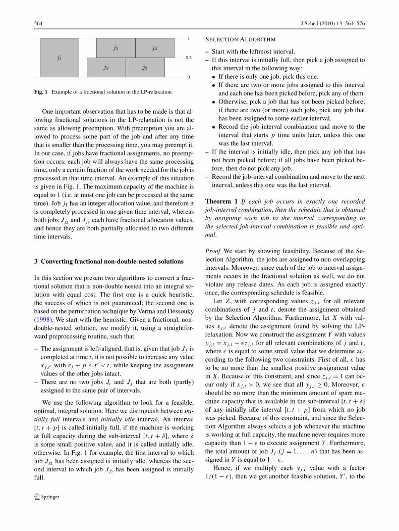
Fig. 1 Example of a fractional solution in the LP-relaxation

One important observation that has to be made is that al-lowing fractional solutions in the LP-relaxation is not thesame as allowing preemption. With preemption you are al-lowed to process some part of the job and after any timethat is smaller than the processing time, you may preempt it.In our case, if jobs have fractional assignments, no preemp-tion occurs: each job will always have the same processingtime, only a certain fraction of the work needed for the job isprocessed in that time interval. An example of this situationis given in Fig. 1. The maximum capacity of the machine isequal to 1 (i.e. at most one job can be processed at the sametime). Job j1 has an integer allocation value, and therefore itis completely processed in one given time interval, whereasboth jobs Jj2 and Jj3 each have fractional allocation values,and hence they are both partially allocated to two differenttime intervals.

3 Converting fractional non-double-nested solutions

In this section we present two algorithms to convert a frac-tional solution that is non-double nested into an integral so-lution with equal cost. The first one is a quick heuristic,the success of which is not guaranteed; the second one isbased on the perturbation technique by Verma and Dessouky(1998). We start with the heuristic. Given a fractional, non-double-nested solution, we modify it, using a straightfor-ward preprocessing routine, such that

– The assignment is left-aligned, that is, given that job Jj iscompleted at time t , it is not possible to increase any valuexj,t ′ with rj + p ≤ t ′ < t , while keeping the assignmentvalues of the other jobs intact.

– There are no two jobs Ji and Jj that are both (partly)assigned to the same pair of intervals.

We use the following algorithm to look for a feasible,optimal, integral solution. Here we distinguish between ini-tially full intervals and initially idle interval. An interval[t, t + p] is called initially full, if the machine is workingat full capacity during the sub-interval [t, t + δ], where δ

is some small positive value, and it is called initially idle,otherwise. In Fig. 1 for example, the first interval to whichjob Jj2 has been assigned is initially idle, whereas the sec-ond interval to which job Jj2 has been assigned is initiallyfull.

SELECTION ALGORITHM

– Start with the leftmost interval.– If this interval is initially full, then pick a job assigned to

this interval in the following way:• If there is only one job, pick this one.• If there are two or more jobs assigned to this interval

and each one has been picked before, pick any of them.• Otherwise, pick a job that has not been picked before;

if there are two (or more) such jobs, pick any job thathas been assigned to some earlier interval.

• Record the job-interval combination and move to theinterval that starts p time units later, unless this onewas the last interval.

– If the interval is initially idle, then pick any job that hasnot been picked before; if all jobs have been picked be-fore, then do not pick any job.

– Record the job-interval combination and move to the nextinterval, unless this one was the last interval.

Theorem 1 If each job occurs in exactly one recordedjob-interval combination, then the schedule that is obtainedby assigning each job to the interval corresponding tothe selected job-interval combination is feasible and opti-mal.

Proof We start by showing feasibility. Because of the Se-lection Algorithm, the jobs are assigned to non-overlappingintervals. Moreover, since each of the job to interval assign-ments occurs in the fractional solution as well, we do notviolate any release dates. As each job is assigned exactlyonce, the corresponding schedule is feasible.

Let Z, with corresponding values zj,t for all relevantcombinations of j and t , denote the assignment obtainedby the Selection Algorithm. Furthermore, let X with val-ues xj,t denote the assignment found by solving the LP-relaxation. Now we construct the assignment Y with valuesyj,t = xj,t − εzj,t for all relevant combinations of j and t ,where ε is equal to some small value that we determine ac-cording to the following two constraints. First of all, ε hasto be no more than the smallest positive assignment valuein X. Because of this constraint, and since zj,t = 1 can oc-cur only if xj,t > 0, we see that all yj,t ≥ 0. Moreover, ε

should be no more than the minimum amount of spare ma-chine capacity that is available in the sub-interval [t, t + δ]of any initially idle interval [t, t + p] from which no jobwas picked. Because of this constraint, and since the Selec-tion Algorithm always selects a job whenever the machineis working at full capacity, the machine never requires morecapacity than 1 − ε to execute assignment Y . Furthermore,the total amount of job Jj (j = 1, . . . , n) that has been as-signed in Y is equal to 1 − ε.

Hence, if we multiply each yj,t value with a factor1/(1 − ε), then we get another feasible solution, Y ′, to the

J Sched (2010) 13: 561–576 565

Fig. 2 Bad example for the Selection Algorithm

LP-relaxation. This implies that X can be written as a con-vex combination of Y ′ and Z; because of the optimality ofX, assignment Z must be optimal, too. �

Unfortunately, the Selection Algorithm does not alwaysproduce a feasible schedule. Consider the following exam-ple (Fig. 2).

All jobs have release date 0, except for jobs Jb and Jc ,the release dates of which coincide with the start points ofthe first intervals they have been assigned to.

If we apply the Selection Algorithm, then we must selectone of the jobs Jd and Jk at time 0, and one of the jobsJi and Jj at time p. Suppose that we have chosen to selectjobs Jd and Jj . At time 2p we select job Ja , since this isa yet unselected job in a partially idle interval. We continuewith Jb at time 3p, job Ji at time 4p, job Jc at time 5p,job Jk at time 6p. At time 7p, we do not select any job,since the interval is partially idle and job Jd has already beenselected. This assignment corresponds to a feasible schedulethat must be optimal according to Theorem 1.

If we alter the initial selection at times 0 and p to jobs Jd

and Ji , then we again select jobs Ja and Jb at times 2p and3p, but at time 4p we are forced to select job Ji again, whichmakes the Selection Algorithm to fail. We might change theSelection Algorithm such that no job is picked at time 2p

(the interval is partially idle, and job Ja must appear lateragain, since it has not been fully assigned yet), pick Jb attime rb , pick job Ja at time rb + p, wait until time 5p topick job Jc, but then we fail at time 6p, since we cannotpick jobs Jj and Jk both, which implies that one of thesejobs will not be selected at all.

Fortunately, Verma and Dessouky (1998) have describeda guaranteed way to convert a fractional solution that isnon-double nested into an integral solution with equal cost.Since each extremal solution is integral, a fractional opti-mal solution must be a convex combination of two or moreextremal solutions with equal cost. To exclude the possi-bility that two extremal solutions have equal cost, Vermaand Dessouky (1998) add a small perturbation to the co-efficients in the objective function; this perturbation is sosmall that an extremal solution to the original problem thatis sub-optimal cannot become optimal for the perturbedproblem. Adding perturbations is done in the following

way:

cj,t = cj,t + jε

where ε is a very small positive number.

4 Common due date

In this section we look at the special case in which all jobsj have a common due date dj = D. Depending upon thesize of D, we distinguish two variants. First, in Sect. 4.1 welook at the case 0 ≤ D < rmin + p, where rmin is the small-est release date of all jobs. For any value of D < rmin + p

we know that each job will be tardy, which implies thatwe obtain an equivalent problem by putting D = 0. The1|rj ,pj = p,dj = 0|∑wjTj problem is equivalent to the1|rj ,pj = p|∑wjCj problem, for which Baptiste (2000)already showed that it can be solved in polynomial time(O(n7)) by means of dynamic programming. In Sect. 4.2 welook at the case where D ≥ rmin + p; in this case it is possi-ble to complete at least one job at or before the due date. Forboth cases we assume without loss of generality that the jobsare re-indexed such that w1 ≤ w2 ≤ w3 ≤ · · · ≤ wn. If afterre-indexing the jobs w1 < w2 < w3 < · · · < wn holds, thenwe say that a strict order on the weight of the jobs exists.

4.1 Common due date equal to zero

Lemma 2 If there exists a strict order on the weight of thejobs, then any optimal solution is nested. When no strictorder exists, then there exists an optimal schedule that isnested.

Proof Assume we have an optimal solution that is doublenested. Therefore, according to Definition 2 there exist jobsJj1 and Jj2 that are nested in each other. Without loss ofgenerality we assume j1 < j2 (i.e. wj2 ≥ wj1 ). Let us nowlook at the situation where job Jj1 is nested in job Jj2 , that is,there exist intervals t1, t2, and t3 such that t1 < t2 < t3 andxj2,t1 , xj1,t2 , and xj2,t3 are all positive (i.e. situation 212).We define ε = min{xj1,t2 , xj2,t3}.

In Fig. 3 an example of the situation 212 is depictedwhere without loss of generality we assumed ε = xj2,t3 . JobJj1 is nested in job Jj2 , and job Jj2 is nested in job Jj1 .

566 J Sched (2010) 13: 561–576

Fig. 3 Example of rearranging ε between two nested jobs.

Since both jobs are tardy, the exchange of ε between xj1,t2

and xj2,t3 causes a change in the cost of Δ, where we have:

Δ = ε(wj2 t2 + wj1 t3 − wj1 t2 − wj2 t3)

= ε(wj2(t2 − t3) + wj1(t3 − t2)

)

= ε((t3 − t2)(wj1 − wj2)

)

≤ 0.

In the resulting situation job Jj2 is still nested in job Jj1 , butjob Jj1 is not nested in job Jj2 anymore. The exchange doesnot violate any constraint as the amount of total allocationat each interval is unaltered, and only its division betweenthe two jobs has been changed. Furthermore, the value ofthe objective function will not increase by this exchange. Incase a strict order exists it can be seen that Δ < 0, whichcontradicts the optimality of the double-nested solution.

If there is no strict order on the weight of the jobs, thenwe may have that Δ = 0 for each of these interchanges.Hence, there can exist an optimal schedule that is doublenested, but we can convert it into a nested schedule withequal cost by repeatedly moving parts of jobs with equalweight, like we did above. �

We have now shown that for the problem 1|rj ,pj =p|∑wjCj a double-nested solution is either optimal (butcan be rewritten into a nested solution with equal cost inpolynomial time) or sub-optimal. Now we can make use ofLemma 1 to show that this problem can be solved in poly-nomial time since the constraint matrix for the non-zerocolumns is totally unimodular. If the LP-solver returns adouble-nested solution, then we first convert it into a nestedsolution as described in the proof of Lemma 2 and, if thisnested solution is fractional, then we apply the Selection Al-gorithm of Sect. 3 to find a feasible schedule with equal cost.If the Selection Algorithm fails, then we can apply the per-turbation technique by Verma and Dessouky.

Solving an LP with n′ variables takes O(√

n′logn′ε) it-

erations of each O(n′3) calculation steps (Roos 2005). Inour case with n jobs, the number of variables we have isO(n3), which means that the total running time for the LP

is O(n10√n log n3

ε). Although in the worst-case this is more

than the previous known result of Baptiste (2000) with dy-namic programming, on average it might be a lot quicker.

4.2 Common due date (dj = D > p)

Now we have the situation that there exists a common duedate for all jobs that is bigger than the first possible comple-tion time of any job. Hence, one or more jobs can be placedbefore the common due date while others will become tardy.

Lemma 3 A double-nested solution is either sub-optimal,or it can be rewritten into a nested solution with equal cost.

Proof Assume that we have an optimal solution that is dou-ble nested. Therefore, there are two jobs Jj1 and Jj2 that arenested in each other; without loss of generality, we assumethat j1 < j2. We address the situation that Jj1 is nested inJj2 . Then there exist time intervals t1, t2, and t3 such thatt1 < t2 < t3 and xj2,t1 , xj1,t2 , and xj2,t3 are positive.

Now there are two distinctions to be made:

– D ≥ t3. In this case the order of the jobs Jj1 and Jj2 doesnot matter because they are both on time. Hence it is pos-sible to switch parts of the jobs around in such a way thatwe end up with a nested solution of equal cost.

– D < t3. If the weights of the two jobs are equal, we canexchange parts between intervals t2 and t3 at no cost toconvert the current double-nested solution into a nestedsolution. Otherwise we use the same approach as in theproof of Lemma 2, and we define ε = min(xj1,t2, xj2,t3).

The optimal way of allocating ε of job Jj2 and ε ofjob Jj1 among the two intervals is to first allocate ε of jobJj2 to interval t2 and then allocate ε of job Jj1 to inter-val t3. The idea behind this can be seen again in Fig. 3.If there exists a strict order on the weights of the jobs,the resulting solution after the exchange will have smallercost. This implies that we can improve or rewrite thedouble-nested solution without violating any constraintsas the amount of total allocation at each interval in unal-tered, and only its division between the two jobs has beenchanged. Furthermore, no job is moved to an interval thatis before any interval it was previously allocated to, andhence each release date is satisfied.

This process might have to be repeated if more occurrencesexist of double-nested situations for these two jobs.

We see that either the double-nested solution is not opti-mal, which contradicts our assumption, or it can be rewritteninto a nested solution of equal cost. �

For the case of equal due dates D with any value for D

we present the following theorem:

Theorem 2 The problem 1|rj ,pj = p,dj = D|∑wjTj

can be solved in polynomial time.

Proof By combining Lemmas 2 and 3 we know that for anyvalue of D there exists an optimal schedule that is nested.

J Sched (2010) 13: 561–576 567

We can then apply the Selection Algorithm to try to convertthis nested, fractional solution to an integral solution withequal cost; if this is unsuccessful, then we apply the pertur-bation technique by Verma and Dessouky (1998). �

5 Arbitrary due dates

Now we look at the situation where all jobs can have dif-ferent due dates. In this case we cannot provide a polyno-mial algorithm for solving the problem, but we give a goodbranching rule that makes use of the structure of the prob-lem.

Unlike the common due date case, with arbitrary duedates a fractional solution of the LP-relaxation can have abetter value than the optimal integer solution. An examplethat shows this is Table 1.

The optimal LP solution with cost 3 is shown in Fig. 4.The possible integral solutions are:

– start with job J1. After that process job J3 and job J4 andfinally process job J2, which will be tardy. This solutionhas cost 5.

– start with job J2. After that one of the jobs J1, J3, andJ4 will become tardy and due to the large weight of thesejobs, the cost of this solution will be greater than 5.

– start with job J3 or J4. Since there is enough of free ca-pacity to put job J1 in front without causing a delay, thisis dominated by the solution in which job J1 is put first.

Thus the optimal ILP solution value equals 5, which is dif-ferent from the optimal LP solution with value 3. Further-more we can see in Fig. 4 that the jobs J1 and J2 are doublenested.

In the following, we will analyze when it can be optimalfor two jobs Jj1 and Jj2 to be double nested; we will fur-ther derive conditions under which we can show that such

Table 1 Common processing time p = 2

Job Release date Due date Weight

1 0 8 100

2 1 3 1

3 2 5 100

4 4 7 100

Fig. 4 Optimal LP solution that is double nested

a double-nested situation is sub-optimal. We number thejobs such that dj1 ≤ dj2 . Anticipating our results, we remarkthat in case of equal due dates a double-nested solution canbe converted into a nested solution. There are two possibledouble-nested situations for the two jobs:

– Situation 1212– Situation 2121

In both cases, we assume that the jobs have been partly as-signed to intervals t1, t2, t3, t4 with t1 < t2 < t3 < t4.

Lemma 4 In the 1212 situation where there are two jobs Jj1

and Jj2 with dj1 ≤ dj2 , a double-nested solution is eithersub-optimal, or it can be rewritten into a nested solutionwith equal cost.

Proof Assume dj2 ≥ t3. In this case job Jj2 will be ontime when completed at time t3. Exchanging ε = min{xj2,t2 ,

xj1,t3} between xj2,t2 and xj1,t3 is profitable or yields thesame cost, since:

– Job Jj2 will still be on time.– Job Jj1 is placed earlier in time and thus its cost can only

decrease or remain the same.

Now assume dj2 < t3. In this case both jobs are tardy attimes t3 and t4. We have to make a distinction into two sep-arate cases, based on the weight of the jobs:

– wj1 ≥ wj2 . A straightforward calculation shows that, be-cause dj1 ≤ dj2 and wj1 ≥ wj2 , the value of the ob-jective function will not increase when exchanging ε =min{xj2,t2, xj1,t3} between xj2,t2 and xj1,t3 .

– wj1 < wj2 . Since both jobs are tardy when completed attime t3, exchanging ε = min{xj1,t3 , xj2,t4} between xj1,t3

and xj2,t4 will increase the cost for job Jj1 by εwj1(t4 − t3)

and decrease the cost for job Jj2 by εwj2(t4 − t3). Sincewj1 < wj2 , the total cost decreases.

Hence, when dj1 ≤ dj2 , the situation 1212 can always berewritten to a nested solution of equal or less cost. �

In the case of dj1 = dj2 we can choose the situation arbi-trarily and thus we can always see it as the 1212-situation.This means that the case of dj1 = dj2 can always be rewrit-ten to a nested solution of equal or smaller cost.

Lemma 5 In the 2121 situation where there are two jobsJj1 and Jj2 with dj1 < dj2 , a double-nested solution is ei-ther always sub-optimal, or it can be rewritten into a nestedsolution of the same cost, unless wj1 < wj2 and rj1 > rj2 .

Proof When wj1 = wj2 , we can always transform the cur-rent solution into a new solution of equal or smaller cost byexchanging between the intervals t3 and t4, since dj1 < dj2 .

568 J Sched (2010) 13: 561–576

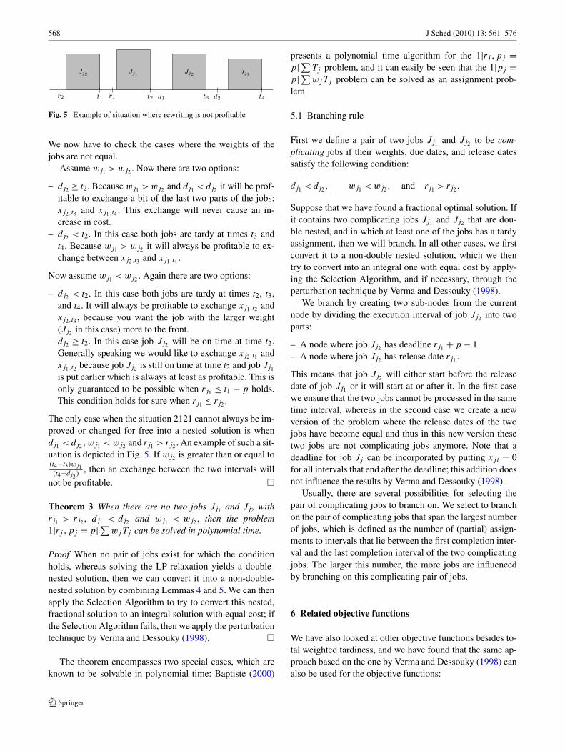
Fig. 5 Example of situation where rewriting is not profitable

We now have to check the cases where the weights of thejobs are not equal.

Assume wj1 > wj2 . Now there are two options:

– dj2 ≥ t2. Because wj1 > wj2 and dj1 < dj2 it will be prof-itable to exchange a bit of the last two parts of the jobs:xj2,t3 and xj1,t4 . This exchange will never cause an in-crease in cost.

– dj2 < t2. In this case both jobs are tardy at times t3 andt4. Because wj1 > wj2 it will always be profitable to ex-change between xj2,t3 and xj1,t4 .

Now assume wj1 < wj2 . Again there are two options:

– dj2 < t2. In this case both jobs are tardy at times t2, t3,and t4. It will always be profitable to exchange xj1,t2 andxj2,t3 , because you want the job with the larger weight(Jj2 in this case) more to the front.

– dj2 ≥ t2. In this case job Jj2 will be on time at time t2.Generally speaking we would like to exchange xj2,t1 andxj1,t2 because job Jj2 is still on time at time t2 and job Jj1

is put earlier which is always at least as profitable. This isonly guaranteed to be possible when rj1 ≤ t1 − p holds.This condition holds for sure when rj1 ≤ rj2 .

The only case when the situation 2121 cannot always be im-proved or changed for free into a nested solution is whendj1 < dj2 , wj1 < wj2 and rj1 > rj2 . An example of such a sit-uation is depicted in Fig. 5. If wj2 is greater than or equal to(t4−t3)wj1(t4−dj2 )

, then an exchange between the two intervals will

not be profitable. �

Theorem 3 When there are no two jobs Jj1 and Jj2 withrj1 > rj2 , dj1 < dj2 and wj1 < wj2 , then the problem1|rj ,pj = p|∑wjTj can be solved in polynomial time.

Proof When no pair of jobs exist for which the conditionholds, whereas solving the LP-relaxation yields a double-nested solution, then we can convert it into a non-double-nested solution by combining Lemmas 4 and 5. We can thenapply the Selection Algorithm to try to convert this nested,fractional solution to an integral solution with equal cost; ifthe Selection Algorithm fails, then we apply the perturbationtechnique by Verma and Dessouky (1998). �

The theorem encompasses two special cases, which areknown to be solvable in polynomial time: Baptiste (2000)

presents a polynomial time algorithm for the 1|rj ,pj =p|∑Tj problem, and it can easily be seen that the 1|pj =p|∑wjTj problem can be solved as an assignment prob-lem.

5.1 Branching rule

First we define a pair of two jobs Jj1 and Jj2 to be com-plicating jobs if their weights, due dates, and release datessatisfy the following condition:

dj1 < dj2, wj1 < wj2, and rj1 > rj2 .

Suppose that we have found a fractional optimal solution. Ifit contains two complicating jobs Jj1 and Jj2 that are dou-ble nested, and in which at least one of the jobs has a tardyassignment, then we will branch. In all other cases, we firstconvert it to a non-double nested solution, which we thentry to convert into an integral one with equal cost by apply-ing the Selection Algorithm, and if necessary, through theperturbation technique by Verma and Dessouky (1998).

We branch by creating two sub-nodes from the currentnode by dividing the execution interval of job Jj2 into twoparts:

– A node where job Jj2 has deadline rj1 + p − 1.– A node where job Jj2 has release date rj1 .

This means that job Jj2 will either start before the releasedate of job Jj1 or it will start at or after it. In the first casewe ensure that the two jobs cannot be processed in the sametime interval, whereas in the second case we create a newversion of the problem where the release dates of the twojobs have become equal and thus in this new version thesetwo jobs are not complicating jobs anymore. Note that adeadline for job Jj can be incorporated by putting xjt = 0for all intervals that end after the deadline; this addition doesnot influence the results by Verma and Dessouky (1998).

Usually, there are several possibilities for selecting thepair of complicating jobs to branch on. We select to branchon the pair of complicating jobs that span the largest numberof jobs, which is defined as the number of (partial) assign-ments to intervals that lie between the first completion inter-val and the last completion interval of the two complicatingjobs. The larger this number, the more jobs are influencedby branching on this complicating pair of jobs.

6 Related objective functions

We have also looked at other objective functions besides to-tal weighted tardiness, and we have found that the same ap-proach based on the one by Verma and Dessouky (1998) canalso be used for the objective functions:

J Sched (2010) 13: 561–576 569

– Total weighted number of late jobs– Total weighted late work

We will discuss both of them in more detail now.When we look at the weighted number of late jobs

problem (1|rj ,pj = p|∑wjUj in the three-field notationscheme), the cost of assigning job Jj to time t is:

cj,t ={

wj if t > dj ,

0 otherwise.

Our approach is again that we solve the LP-relaxation and,if fractional, try to convert the solution into a non-double-nested one with equal cost from which we then derive anoptimal integral solution. Unfortunately, a solution in whichJj1 and Jj2 are nested in each other can be better than anon-double-nested solution in case dj1 < dj2 and rj1 > rj2 ,and we have to branch then. Baptiste (1999) presents a dy-namic programming algorithm that solves this problem inpolynomial time (O(n7)). Although according to the worst-case running time our algorithm might not perform as well,on average it could be very competitive since in case ofdynamic programming the average and worst-case runningtimes are equal.

We apply the same analysis as in Sect. 5 to remove doublenestings, if possible. Suppose that the jobs Jj1 and Jj2 aredouble nested. The proofs for Lemmas 4 and 5 also hold forthis objective function with the following two changes:

– In some of the cases there is not a strict decrease in costby exchanging between two intervals, but the resultingschedule after the exchange will have equal cost. This isdue to the binary character of this objective function.

– The case where wj1 ≥ wj2 cannot always be rewritten inthe 2121 situation. The reason for this is again the bi-nary character of the objective function. In case of totalweighted tardiness an exchange between two tardy inter-vals never increases the objective function, since dj1 isstrictly smaller than dj2 . In case of weighted number oflate jobs it is not guaranteed that this exchange does notincrease the objective function. An example of a situationwhere the objective function increases is the same as theone depicted in Fig. 5 in Sect. 5. An exchange betweenthe last two intervals will increase the cost because jobJj1 will still be tardy and job Jj2 will become tardy af-ter the exchange. An exchange between the middle twointervals will also increase the cost since job Jj1 will be-come tardy while job Jj2 will still be on time after theexchange.

We see that regardless of the weights, the 2121 situation can-not always be rewritten. Therefore, we have to redefine thedefinition of complicating jobs for this objective function asfollows. A pair of two jobs Jj1 and Jj2 are complicating jobs

if their due dates and release dates satisfy the following con-dition:

dj1 < dj2 and rj1 > rj2 .

We need to extend the branching rule a little. From ourexperiments we saw that some instances took very long tosolve. Looking at the branching information we saw that thiswas caused by jobs with a small time interval for being ontime (i.e. a job Jj with dj −rj < 2p). If such a job Jj existedand was partially assigned to an on-time interval and a tardyinterval, then job Jj would be always selected for possiblebranching with another job Jj ′ , where Jj and Jj ′ are a pairof complicating jobs. To try and prevent such unnecessarybranching, we changed the branching rule in the followingway: In a node we first check whether there exists a job Jj

with dj − rj < 2p and both tardy and non-tardy completiontimes. If such a job exists, we create two child nodes fromthe current node:

– A child node where job Jj will be on time (dj is turnedinto a deadline);

– A child node where job Jj will be tardy (the release dateis increased to dj − p + 1).

If such a job does not exist, we go on with the earlier sug-gested branching rule.

When we look at the weighted total late work problem1|rj ,pj = p|∑wjVj , the cost for assigning a job Jj totime t is:

cj,t ={

wjpj if t ≥ dj + p,

wj max(0, t − dj ) otherwise.

Since this objective in its most extreme form (when Cj >

dj + p for a job Jj ) behaves similarly to the weighted num-ber of late jobs (cost will not increase anymore by placingjob Jj even later), we find that also for this objective func-tion we cannot guarantee that the 2121 situation can alwaysbe rewritten into a nested solution of equal or smaller cost;the counterexample is the same as the one given for the sumof weighted late jobs, depicted in Fig. 5. This means that alsofor this objective function we have to redefine the definitionof complicating jobs in the same way as for the weightednumber of late jobs.

For both of these objective functions the case where therelease dates and the due dates are equally ordered meansthat no complicating jobs can exist, which means that thesolution to the LP-relaxation will either be already integral,or the fractional solution can be converted to an integral so-lution of same cost. This means that the cases where such anequal ordering exists are polynomially solvable.

570 J Sched (2010) 13: 561–576

7 Parallel identical machines

A nice advantage of the time-indexed formulation is that itcan be used to solve problems with m parallel, identical ma-chines as well. In this machine environment, there are m ma-chines available, and processing job Jj can be done by anyone of these machines, which takes an uninterrupted periodof length pj = p independent of the machine that executesit. We can formulate the problem as an ILP problem by us-ing assignment variables xj,t , which model our decision ofexecuting job Jj in period t . The only difference with thesingle-machine variant is that we now can process m jobs atthe same time, which we can model by adjusting the right-hand side in constraint (2) from 1 to m. This leads to thefollowing ILP-formulation:

min z =n∑

j=1

∑

t∈Aj

cj,t xj,t

subject to

∑

t∈Aj

xj,t = 1 for all j ∈ N , (4)

n∑

j=1

∑

t ′∈Ht∩Aj

xj,t ′ ≤ m for all t ∈ K ∪ G, (5)

xj,t ∈ {0,1} for all j ∈ N , t ∈ Aj . (6)

It is readily verified that any integral solution can be con-verted into a feasible schedule by greedily assigning job Jj

to any machine that is available in the period t for whichxj,t = 1.

Since the constraint matrix has not been changed,Lemma 1 still holds. Hence, we come to the following corol-lary.

Corollary 1 If any double-nested solution to the LP-relaxation is either sub-optimal or can be rewritten to anested solution with equal cost, then there exists an optimalsolution to the LP-relaxation that is integral.

Since the proofs that we have given in the Sects. 4, 5,and 6 to show how to modify double-nested solutions donot depend on the number of machines involved, it followsthat all our previous results concerning double-nested so-lutions still hold. Therefore, the only thing left to do isto find the integral optimal solution in case that solvingthe LP-relaxation yields a fractional one. Unfortunately, theheuristic presented in Sect. 3 for the single-machine caseto convert a nested, fractional solution into an integral so-lution with equal cost could not be generalized to the m-machine case. Therefore, we immediately apply the pertur-bation method presented by Verma and Dessouky (1998).

8 Column generation

A big disadvantage of our time-indexed formulation is that ituses huge amounts of memory. For the biggest of the prob-lems we tested memory usage was in the order of about 1.7Gigabyte. To see if it was possible to reduce the amount ofmemory needed for solving the problems we looked at col-umn generation.

The idea here is to split up the time horizon into B timeframes. These time frames do not necessarily need to havethe same length but must have a length ≥ p −1. This idea ofdividing the complete time horizon has been independentlysuggested by Bigras et al. (2005) for solving the 1 ‖ wjTj

problem by means of column generation. All time framescombined should cover the complete time horizon com-pletely, and consecutive time frames may overlap at mostp − 1 time units. Each time frame b (b = 1, . . . ,B) hasa start time μb and end time ωb . Without loss of general-ity we created the time frames in such a way that two con-secutive time frames have an overlap of exactly p − 1 (i.e.μb+1 + p − 1 = ωb).

Given a division of the time horizon into a set of timeframes, we compute for each time frame a feasible schedulefor a subset of the jobs, such that each job is executed in ex-actly one time frame. We formulate this problem as an ILPusing the concept of time-frame plans. A time-frame planfor a given time frame consists of the completion times fora subset of the jobs. The completion times must be feasi-ble within the time frame, meaning that the jobs can actu-ally be completed at their respective completion times, andall completion times must lie within the boundaries of thetime frame. Now we need to find a suitable time-frame planfor each of the time frames. We need to make sure that alljobs are processed in exactly one of the selected time-frameplans. Furthermore, we also have to make sure that the totalidle time in the overlapping part of two consecutive time-frame plans is greater than or equal to p − 1, ensuring thatwe do not violate the capacity constraint in the overlappingpart.

Let s denote the number of possible time-frame plans.For each time-frame plan i we determine the indicators yji

and qbi , which are defined as

yji ={

1 if job Jj is processed in time-frame plan i,

0 otherwise,

qbi ={

1 if time-frame plan i is for time-frame b,

0 otherwise.

We denote the cost of time-frame plan i by ci , and we useyi and zi to denote the amount of idle time in the front andend overlap of the time frame. We introduce the binary vari-able xi to indicate whether or not we include time-frame

J Sched (2010) 13: 561–576 571

plan i in our solution. Now the complete ILP model is asfollows:

mins∑

i=1

cixi

subject to

s∑

i=1

yjixi = 1, j = 1 . . . n, (7)

s∑

i=1

qbixi = 1, b = 1 . . .B, (8)

s∑

i=1

ziqbixi +s∑

i=1

yiqb+1,ixi ≥ p − 1, b = 1 . . .B − 1,

(9)

xi ∈ {0,1} ∀i. (10)

Constraint (7) ensures that all jobs will be present in exactlyone selected time-frame plan and constraint (8) ensures thatfor each time-frame exactly one time-frame plan will be se-lected. Finally constraint (9) ensures that the idle time in theoverlap between two consecutive time-frame plans is at leastp − 1.

To approximate the optimum of this integral model, wefirst relax the integrality constraint (10) to xi ≥ 0 (theother constraints ensure xi ≤ 1). We solve the resulting LP-relaxation through column generation.

In each iteration we only allow a subset of the time-frameplans and solve the LP-relaxation for this restricted set ofvariables. We then solve the corresponding pricing prob-lem to find out whether there are time-frame plans the ad-dition of which will reduce the objective function. The pric-ing problem is defined as finding the feasible time-frameplan with minimum reduced cost; if this minimum is non-negative, then we have solved the LP-relaxation to optimal-ity. To compute the reduced cost we need the dual multipli-ers.

For each type of constraint in the master problem we geta dual multiplier:

– From (7) we get a dual multiplier πj for each job Jj .– From (8) we get a dual multiplier τb .– From (9) we get a dual multiplier φb for each overlap be-

tween time frame b and b + 1.

We solve the pricing problem for each time frame individ-ually. It can be solved in a similar fashion as the originalproblem: for a given time frame we define the set of possi-ble completion times and then assign these to eligible jobssuch that the capacity constraints are satisfied. The changes

that have to be made for solving the pricing problem for agiven time frame b are:

– We can discard any completion time < μb + p or > ωb

and create the following sets:• Ab

j = {a ∈ Aj |μb + p ≤ a ≤ ωb} (j = 1, . . . , n) denot-ing the possible completion times of job Jj within timeframe b.

• Hbt = {h ∈ Ht |μb ≤ h ≤ ωb + p} ∀t denoting the time

indices within time frame b that are conflicting withtime t .

• Gb = {g ∈ G|μb ≤ g ≤ ωb + p} denoting all first pos-sible completion times of all jobs within time frame b.

• Kb = {k ∈ K|μb ≤ k ≤ ωb +p} denoting all other pos-sible completion times of all jobs that are within timeframe b.

– We are interested in jobs that are processed in the timeframe b. Possibly not all jobs can be processed, so werelax the constraint ‘all jobs must be processed exactlyonce’ to ‘all jobs must be processed at most once’.

– Since we need to know something about the available idletime in the overlapping regions, we add two extra jobs αb

and βb , both with processing time p, for the front over-lap and the end overlap of a time frame respectively. Thepossible completion times for these two extra jobs are:• Ab

α : {μb,μb + 1, . . . ,μb + p − 1}.• Ab

β : {ωb + 1,ωb + 2, . . . ,ωb + p}.It can be seen that these jobs have a special status, sincejob α starts before the start time of the time frame and jobβ ends after the end time of the time frame. For the firsttime frame job α does not exist and for the last frame jobβ does not exist because there is no time frame to overlapwith.

Solving the pricing problem should result in a time-frameplan with minimum reduced cost. Hence, we need to set thecost of job Jj being completed at time t such that it corre-sponds exactly to its contribution to the reduced cost. If a jobJj is not assigned in this time frame, it does not contributeto the cost function; otherwise, the cost cj,t of assigning jobJj to time t is defined as follows:

cj,t = wj max{0, t − dj } − πj .

Furthermore the cost for assigning the αb and βb jobs to atime t are as follows:

cαb,t = (t − μb)φb+1,

cβb,t = (ωb + p − t)φb,

which corresponds to the amount of idle time at the front orthe back of the time frame multiplied by the correspondingdual multiplier.

572 J Sched (2010) 13: 561–576

The pricing problem we need to solve for a certain timeframe b is as follows:

minn∑

j=1

∑

t∈Abj

cj,t xj,t − τb −∑

t∈Abβ

cβb,t xβb,t −∑

t∈Abα

cαb,t xαb,t

subject to

∑

t∈Abj

xj,t ≤ 1 for all j ∈ N , (11)

∑

t∈Abα

xαb,t = 1, (12)

∑

t∈Abβ

xβb,t = 1, (13)

n∑

j=1

∑

t ′∈Hbt ∩Ab

j

xj,t ′ +∑

t ′∈Hbt ∩Ab

α

xαb,t′ +

∑

t ′∈Hbt ∩Ab

β

xβb,t′ ≤ 1

for all t ∈ Kb ∪ Gb, (14)

xj,t ∈ {0,1}, for j ∈ N ∪ {α,β}, t ∈ Abj . (15)

Constraint (11) ensures that all regular jobs are processedat most once and constraint (12) and constraint (13) ensuresthat the alpha and beta job are processed exactly once. Fi-nally constraint (14) ensures that there does not exist a timewhere more than one job is processed.

When the pricing problem is solved we know which jobsare assigned to which time intervals and we can calculatethe cost ci of the new variable xi in the master problem asfollows

n∑

j=1

∑

t∈Abj

cj,t xj,t .

Furthermore the two indicators yi and zi denoting the idletime in the front overlap region and the rear overlap regioncan be set according to the assignment of the α and β job.

For creating the initial variables for the master problemwe ordered the jobs on their release dates and assigned themto the earliest possible time interval. From this integral fea-sible schedule we determined which jobs were processedin which time intervals and from this we created the ini-tial variables. When the LP-relaxation is solved to optimal-ity with the column generation, we add the integrality con-straint back again to the master problem and then try tosolve the master problem again with the generated set ofcolumns.

Initial tests with a prototype implementation showed thatthe solutions given by solving the LP-relaxation with col-umn generation often had a fractional solution value lower

than the integral solution we found with our initial repre-sentation. As expected, the total amount of memory neededfor solving the problems was a lot less because only a smallpart of the total number of variables was created in memory.One major disadvantage the tests showed was that the run-ning time for solving the LP-relaxation to optimality grewconsiderably. However, since the problem is divided intoa set of smaller, independent, subproblems, we can easilyparallelize the solving of the subproblems. Since this LP-relaxation gave a lot weaker lower bound, one approach tosolve the ILP problem to optimality would be to make useof branch-and-price. We did not implement this.

9 Computational experiments

For testing the time-indexed formulation, the branching rule,and the Selection Algorithm a program was written in Java.All tests were run on a Pentium 4 running at 3.00 GHz with1 GB of RAM. For solving the ILPs we used Cplex 9.1(ILOG 2005). We wanted to create some problems varyingin size and did this by choosing the number of jobs n fromthe set {70,80,90,100} and the common processing time p

from the set {5,10,15,20,25,30}. For each combination ofthese two parameters we created 50 instances in the follow-ing way:

– rj was randomly selected from the interval [0, (n − 6)p).– wj was randomly selected from the interval [0,120).– dj was randomly selected from the interval [rj + p,

(n − 5)p).

This resulted in a total of 1200 instances. Each of these in-stances was then solved for the three objective functions sumof weighted tardiness, sum of weighted late jobs, and sum ofweighted late work.

The results of the tests for the weighted tardiness problemcan be found in Table 2. The first two columns denote thenumber of jobs and the common processing time. The nexttwo columns give the average time in milliseconds neededfor solving the instances by using pure Cplex without anyextra information in the first column and by using Cplex en-hanced with the branching rule and Selection Algorithm inthe second. The following two give the average number ofnodes that needed to be explored before the optimum wasfound. The next two give the average number of iterationsneeded before the problem was solved to optimality. The fi-nal column gives the average integrality gap for the set ofinstances.

One thing that can be clearly seen from the table is thatthe average integrality gap is very little to completely non-existent, denoting that the relaxed time-indexed formulationgives a really strong bound for the solution. This can also beseen by looking at the average number of nodes that neededto be explored before the optimum was found.

J Sched (2010) 13: 561–576 573

Table 2 Results weighted tardiness

Jobs P Average time for solving (ms) Average number of nodes Average number of iterations Averageintegralitygap (‰)Cplex B.R. Cplex B.R. Cplex B.R.

70 5 1891.60 1573.10 0.12 0.00 985.08 944.72 0.8

70 10 4780.08 4036.70 0.00 0.00 1721.20 1641.18 =70 15 10220.30 6946.68 0.14 0.00 2021.24 1853.60 0.0

70 20 14435.70 10444.10 0.16 0.00 2364.98 2213.54 =70 25 19684.76 15678.44 0.22 0.04 2721.16 2562.24 0.1

70 30 27206.66 17545.42 0.82 0.04 2897.80 2584.78 0.2

80 5 2840.56 2264.26 0.48 0.00 1334.74 1251.34 0.2

80 10 7877.82 5957.82 0.00 0.00 2002.34 1876.98 0.0

80 15 14807.52 10731.10 0.10 0.00 2454.92 2304.52 0.2

80 20 27111.76 16999.60 0.30 0.00 3043.64 2756.76 0.0

80 25 36674.16 20459.46 0.48 0.00 3236.98 2804.32 =80 30 37105.58 25986.88 0.24 0.02 3363.52 3075.04 0.2

90 5 4144.52 2926.86 0.00 0.00 1527.34 1404.26 0.0

90 10 13632.42 9153.16 0.20 0.02 2458.74 2251.18 0.1

90 15 25802.94 15212.90 0.40 0.00 3146.56 2758.06 =90 20 37260.04 23841.70 0.32 0.00 3578.20 3257.10 =90 25 47910.14 31606.50 0.20 0.00 3939.44 3579.86 =90 30 72489.82 42054.82 0.80 0.00 4322.44 3817.04 =

100 5 5153.96 4183.32 0.00 0.00 1754.06 1674.80 0.0

100 10 16928.82 12230.32 0.30 0.00 2805.62 2608.72 =100 15 32375.18 23278.04 0.18 0.00 3566.20 3346.54 0.0

100 20 61929.32 34486.50 1.02 0.00 4463.46 3873.96 =100 25 100738.12 50501.48 1.12 0.00 5326.60 4302.40 0.0

100 30 122807.82 75730.52 0.44 0.08 5655.16 4979.72 0.2

Cplex = Results Cplex 9.1, B.R. = Results with branching rule and Selection Algorithm = : Integrality gap was 0 for all instances

If we look at the first line (70 jobs with P = 5) in Table 2we see that with the branching rule and Selection Algorithmon average 0 nodes need to be explored before the optimumis found, while there still is an integrality gap. The reasonfor this is that after solving the root node, Cplex added somecuts, after which the Selection Algorithm could convert thenew solution to an integral solution. In the majority of theinstances, after Cplex finished solving the root-node LP andpossibly added some cuts, the Selection Algorithm couldconvert the found fractional solution to an integral solutionof same cost. In the cases the Selection Algorithm could notbe applied, the number of nodes that needed to be exploredto find the optimum never exceeded 4. The number of nodesthat were explored when only Cplex was used was at most30 and for all instances this number was always greater thanor equal to the number of nodes needed with the branchingrule and Selection Algorithm.

The results for the objective functions weighted late jobsand weighted late work can be found in Tables 3 and 4 re-spectively.

If we look at these two tables then we see that forsome of the problems, Cplex on average needs to explorefewer nodes before the optimum is found than our branch-and-bound algorithm. In all cases this increased average iscaused by a single instance for which our branching rulebranches on an unfortunate set of variables. This causes a lotof nodes to be explored before the optimum can be found.

Another observation is that for the number of weightedlate jobs problem, for two of the sets of larger instances thereexist instances that Cplex could not solve. Initially these in-stances were not solvable with the original branching ruleeither; only after changing the branching rule as mentionedin Sect. 6 these instances could be solved.

The implementation was not optimized for speed andsome improvements are still possible. These changes would

574 J Sched (2010) 13: 561–576

Table 3 Results weighted late jobs

Jobs P Average time for solving (ms) Average number of nodes Average number of iterations Averageintegralitygap (‰)Cplex B.R. Cplex B.R. Cplex B.R.

70 5 2173.76 1614.40 0.28 0.00 925.26 824.52 19.0

70 10 6336.38 4704.88 0.22 0.04 1584.54 1410.76 5.2

70 15 15812.24 9536.66 24.12 0.18 1852.96 1590.34 11.9

70 20 19019.84 14309.14 2.08 4.06 2177.22 2005.26 7.1

70 25 32457.72 20199.04 33.20 0.14 2592.64 2149.72 18.1

70 30 32067.36 21591.08 0.50 0.10 2335.52 2082.78 4.0

80 5 4115.68 2787.94 17.38 0.14 1251.30 1098.20 14.1

80 10 11372.56 6780.58 14.86 0.04 1903.24 1623.14 1.3

80 15 19108.02 11399.24 0.36 0.00 2292.64 1943.30 0.8

80 20 39983.62 21466.40 23.50 0.34 2880.24 2369.90 23.1

80 25 57937.80 38194.18 2.58 0.36 3281.24 2534.72 13.1

80 30 56392.76 45024.90 2.48 15.24 3182.84 3000.28 4.7

90 5 5204.18 3042.52 0.56 0.00 1436.70 1226.82 11.6

90 10 18414.40 9015.18 1.04 0.00 2364.08 1901.80 3.5

90 15 45076.90 21474.64 19.16 0.12 3167.76 2452.88 17.0

90 20 55830.74 29861.64 0.94 0.18 3482.40 2812.38 12.9

90 25 96773.20 44125.78 40.16 0.14 4263.70 3109.56 0.9∗90 30 210834.68 74404.14 365.88 0.60 6117.14 3750.76 23.2

100 5 6671.16 4945.88 1.38 0.10 1683.70 1495.80 9.0

100 10 36198.62 18203.18 48.52 0.20 3201.30 2416.08 10.9

100 15 53255.30 26856.22 1.64 0.04 3546.68 2911.34 7.3

100 20 125703.80 44362.66 3.72 0.24 4959.40 3313.70 13.9

100 25 189431.78 78217.88 356.50 0.84 7652.92 4092.86 4.2∗100 30 374531.18 173092.26 326.68 1.04 11306.32 5049.76 21.4

Cplex = Results Cplex 9.1, B.R. = Results with branching rule and Selection Algorithm, ∗Cplex could not solve one or more instances

not improve the number of nodes or number of iterationsfor any of the problems, but would only decrease the timeneeded for solving the problems. The more nodes that needto be explored, the bigger the decrease in time would be.

Another observation that was made during the tests, isthat the memory needed by pure Cplex was on average con-siderably more compared to the memory consumption ofCplex combined with our branching rule. This can be ex-plained by the fact that Cplex branches on single variables,while our branching rule branches on a set of variables andthus the branching depth stays lower.

10 Conclusion and further research

Our basis problem is the 1|rj ,pj = p|∑wjTj problem.We have presented a time-indexed ILP-formulation for this

problem and show that if the instance does not contain twojobs Ji and Jj such that di < dj and wi < wj and wi < wj

then the LP-relaxation can be converted into an optimal so-lution. For the general case we present an efficient branch-and-bound algorithm.

Next, we showed that the same approach could beused for the single-machine problems of minimizing totalweighted late work and total weighted late jobs, respec-tively. Here the LP-relaxation can be converted into an op-timal solution in case the release dates and due dates areequally ordered.

We further showed that the results obtained for the single-machine problems can directly be translated to the corre-sponding problems with m identical, parallel machines, ex-cept for that we could not generalize the single-machine Se-lection Algorithm to the m-machine situation. This can becircumvented by using small perturbations in the cost func-tion.

J Sched (2010) 13: 561–576 575

Table 4 Results weighted late work

Jobs P Average time for solving (ms) Average number of nodes Average number of iterations Averageintegralitygap (‰)Cplex B.R. Cplex B.R. Cplex B.R.

70 5 2080.66 1489.94 0.00 0.00 901.72 816.60 0.9

70 10 5456.00 3844.50 0.00 0.00 1534.30 1380.56 1.3

70 15 12834.56 7676.14 10.92 0.04 1868.04 1636.96 1.0

70 20 16126.78 10842.42 0.12 0.40 2077.12 1876.96 0.4

70 25 30571.46 19438.82 21.00 0.22 2511.44 2217.86 3.1

70 30 28914.50 18249.92 2.86 0.24 2495.60 2169.92 3.7

80 5 3395.70 2322.50 0.54 0.08 1237.94 1081.62 0.9

80 10 10167.48 6547.82 0.36 0.02 1971.60 1695.80 1.2

80 15 16948.26 11093.56 0.24 0.06 2254.70 2026.52 0.2

80 20 27690.58 17443.74 0.28 0.08 2679.92 2351.72 0.8

80 25 73342.68 31503.12 60.88 0.24 3513.04 2628.76 3.3

80 30 59537.10 26996.18 45.68 0.22 3220.96 2599.38 0.7

90 5 5406.16 2836.42 1.26 0.00 1463.48 1228.06 0.2

90 10 17117.94 10031.40 1.06 0.34 2462.54 2007.40 1.1

90 15 31236.90 15361.46 0.72 0.00 2821.76 2371.84 0.2

90 20 55840.70 24638.02 0.80 0.00 3455.44 2759.28 0.0

90 25 74709.72 34966.28 12.50 0.28 3983.92 3074.80 1.2

90 30 100073.20 48197.24 1.28 0.06 4391.50 3459.70 1.0

100 5 5781.44 4375.96 0.68 0.06 1617.74 1468.30 4.4

100 10 29789.30 13383.64 5.40 0.06 3111.58 2428.16 4.2

100 15 46590.86 32824.52 1.30 1.50 3574.30 3086.56 1.4

100 20 95535.26 36192.38 1.96 0.08 4732.06 3283.82 2.3

100 25 184365.38 67680.54 3.98 0.42 6221.94 4079.94 0.9

100 30 181203.72 84013.28 3.24 0.48 5599.68 4349.68 2.8

Cplex = Results Cplex 9.1, B.R. = Results with branching rule and Selection Algorithm

Finally, we have shown that the technique of column gen-eration can be used to solve this kind of problems in case ofa lack of memory to perform the standard ILP algorithm.

There are three clear open questions. The first one isto establish the computational complexity of 1|rj ,pj =p|∑wjTj ? Although we have given a good characteriza-tion of the problem, it is still an open question whetherthe general 1|rj ,pj = p|∑wjTj problem is polynomiallysolvable. The second question is to devise a fast, exact algo-rithm to convert a fractional, nested solution to an integralsolution. The third question is to determine a heuristic orexact algorithm to convert a fractional, nested solution to anintegral solution for the m-machine case.

Acknowledgements The authors want to express their gratitude toChams Lahlou. As a referee, he gave very useful comments on an ear-lier draft of the paper in which he showed by example (which example

we copied in Fig. 2) that the Selection Algorithm is just a heuristic.The research of the second author was conducted when he was a Ph.D.-student at Utrecht University.

Open Access This article is distributed under the terms of the Cre-ative Commons Attribution Noncommercial License which permitsany noncommercial use, distribution, and reproduction in any medium,provided the original author(s) and source are credited.

References

Akturk, M. S., & Ozdemir, D. (2001). A new dominance rule to min-imize total weighted tardiness with unequal release dates. Euro-pean Journal of Operational Research, 135, 394–412.

Baptiste, P. (1999). Polynomial time algorithms for minimizing theweighted number of late jobs on a single machine with equalprocessing times. Journal of Scheduling, 2, 245–252.

Baptiste, P. (2000). Scheduling equal-length jobs on identical parallelmachines. Discrete Applied Mathematics, 103(1–3), 21–32.

576 J Sched (2010) 13: 561–576

Baptiste, P., Brucker, P., Knust, S., & Timkovsky, V. (2004). Ten noteson equal-processing-time scheduling. 4OR: Quarterly Journal ofthe Belgian, French and Italian Operations Research Societies, 2,111–127.

Bigras, L.-P., Gamache, M., & Savardan, G. (2005). Time-indexed for-mulations and the total weighted tardiness problem. Technical re-port, GERAD and ’Ecole Polytechnique de Montréal.

Du, J., & Leung, J. Y. T. (1990). Minimizing total tardiness on onemachine is NP-hard. Mathematics of Operations Research, 15(3),483–495.

Graham, R. L., Lawler, E. L., Lenstra, J. K., & Rinnooy Kan,A. H. G. (1979). Optimization and approximation in deterministicsequencing and scheduling: a survey. Annals of Discrete Mathe-matics, 5, 287–326.

ILOG (2005). ILOG CPLEX v9.1, http://www.ilog.fr.

Lawler, E. L. (1977). A pseudopolynomial algorithm for sequencingjobs to minimize total tardiness. Annals of Discrete Mathematics,1, 331–342.

Lenstra, J. K., Rinnooy Kan, A. H. G., & Brucker, P. (1977). Complex-ity of machine scheduling problems. Annals of Discrete Mathe-matics, 1, 343–362.

Leung, J. Y.-T. (2004). Handbook of scheduling. New York: Chapmann& Hall/CRC.

Nemhauser, G. L., & Wolsey, L. A. (1988). Integer and combinator-ial optimization. Wiley-interscience series in discrete mathematicsand optimization. New York: Wiley.

Roos, C. (2005). Private communication.Verma, S., & Dessouky, M. (1998). Single-machine scheduling of unit-

time jobs with earliness and tardiness penalties. Mathematics ofOperations Research, 23(4), 930–943.