i

Eindhoven, March 2011

BSc Industrial Engineering — Bilkent University 2007 Student identity number 0677327

in partial fulfilment of the requirements for the degree of

Master of Science in Operations Management and Logistics

Supervisors: Ir. Dr. S.D.P. Flapper Dr. T. van Woensel Marc van Pruijssen, Access Business Group Dennis Triepels, Access Business Group

Minimizing Total Supply Chain Costs while Maintaining the Required Service Levels at Access Business Group by Tuba Uluc

ii

TUE. Department Technology Management. Series Master Theses Operations Management and Logistics Subject headings: Multi-Echelon, Inventory Control, Periodic Review, Demand Uncertainty, Lost Sales, Safety Stock, Service Level, Lead Time

iii

ABSTRACT

In this master thesis, an inventory planning tool for the direct selling industry is developed. The aim

is to minimize total supply chain costs while maintaining the required service levels. For that

purpose, alternative inventory policies are developed. The effects of applying alternative policies are

analyzed in terms of P3 service levels, safety stock levels and total inventory carrying costs. The

models offered here are further extended with different scenarios and new perspectives. Finally,

further extension options are presented.

iv

PREFACE This Master Thesis document presents the result of my graduation project for the Master of Science

program in Operations Management and Logistics at Eindhoven University of Technology. This study

was carried out six months from September 2011 to February 2011 at Access Business Group in

Venlo, Netherlands.

I have completed this master thesis with the support and motivation of many people. First of all, I

would like to thank my primary supervisor from TU/e, Dr. Simme Douwe Flapper for his contribution

to this project. His feedbacks, guidance and professional support were very valuable for me. Without

his refreshing insights and incessant care, this project would not be possible. Additionally, I would

like to thank my second supervisor Dr. T. van Woensel for his feedbacks and opinions.

Within ABG, I would like to thank Marc van Pruijssen and Dennis Triepels for giving me the

opportunity to work on this project in their company. Dennis Triepels did his best to attend my

needs. I want to thank Mark Basten, Joop Zanders, Mark Huijs, Tino van Dijck and Stefan Piebinga for

their useful guidance throughout the project. Also, I would like to thank my other colleagues in ABG

for their ever-lasting smiles, and incredible warmness, which they have never spared from me.

Additionally, I would like to thank Amway USA members for their guidance on my research

dimensions. Some important data that the thesis includes has been generously provided by Amway.

Especially David Tackman and Hongjinn Park have tried to respond all my questions.

I also want to thank to people who are not directly involved in this project. I would really like to

thank my friends Recep Meric Gungor and Hande Koc. Their support, invaluable contributions and

empathy were with me whenever needed. They reminded me the most indispensable human values

such as unselfish support and unconditional empathy.

I would like to thank my friends Berna Celebi Kalk and Ulku Guner for motivating me, and

contributing to my morale. And thanks to my friend, Aysegul Demirtas. In my lonely days in

Eindhoven, I found her warm heart. She became my friend, neighbor, and family in an otherwise

lonely some city. Her friendship was a source of intellectual and emotional strength for me. Thanks

to Naz Olgun, who became a sister for me during the four years of our friendship. She made long

distances meaningless and shared every moment of my life in Eindhoven.

Thanks to my ever-lasting friendships with 8 beautiful women from Bilkent University, Ankara. They

added joy, love, smiles, and beauty to my life. Their separate, but all colorful souls have a mind-

altering effect on me. We collected so many cherishable memories, and they will be never forgotten.

I also want to express my deepest gratitude to my parents, Gulcin Uluc and Duzgun Uluc, for being

there for me by any means possible throughout my entire life and for their unconditional love. I am

also thankful to my brother Serdar Uluc for being a source of joy, mentoring me in how to fight

against my own fears, and to develop self-confidence. Without them, life would be unbearable.

Tuba Uluc, March 2011

v

MANAGEMENT SUMMARY

The core function of supply chain planning models is to coordinate material and resource release

decisions in the supply chain in a way that predefined customer service levels are achieved with

minimal costs. According to the 17th Annual State of Logistics Report, business logistics cost as a

percentage of US gross domestic product has grown to 9.5 percent, and of the over $1 trillion spent

on logistics, approximately 33 percent can be attributed to the cost of holding inventory (Williams

and Tokar, 2008). Therefore, inventory management is important for the companies.

This project has been done in the Access Business Group (ABG). The company has recently, changed

its focus from availability into availability with lower stock. This change indicates that ABG wants to

lower stock levels in the overall supply chain while meeting the service level targets. Main research

question is stated as follows:

“How to minimize total supply chain costs while maintaining the required service levels?”

When we checked the realized (actual) service levels, we observed that they are well above the

target levels. The potential problem to be checked is that the current inventory levels are higher

than the necessary levels, which may have been resulting in high supply chain costs. There were two

options to investigate for the cause of high levels of inventory: forecast accuracy and inventory

policy. In this study, we did not deal with the forecast accuracy because it is Amway driven. It is not

controlled by ABG. Therefore, we moved up the study into the inventory policy. We examined the

present inventory policy and deal with its problematic parts in order to align the realized service

levels with the target values.

As the first step, we studied the present planning and control structures for the total supply chain.

Then, we conducted a pilot study on a single item (E0001 Multi-purpose cleaner) and end market

combination (Russia). We focused on the standard inventory flows in this project. We ignored the

manual flows which are applied in the case of emergencies. With the help of an explicit translation

of what ERSC Venlo planners are doing implicitly, the problem is simplified from a multi-echelon

setting to a single echelon setting.

In order to select an appropriate inventory policy, we analyzed the supply and demand processes of

the selected item. We have found that demand pattern is non non-stationary. Although

deterministic lead times are used in the company’s information planning system, it is observed that

actual transportation times fluctuates highly. According to the results of the analysis of the supply

and demand processes, it is found that the problem in our case has the following characteristics:

A single echelon setting,

Non-stationary demand pattern,

Variable lead times,

Lost sales, and

P3 service level.

We reviewed the literature, but we could not find a study that matches our study with respect to the

characteristics of the problem. It was not possible to find inventory policies that are appropriate for

the combination of non-stationary demand, lost sales and P3 service level. Therefore, we proposed

vi

case specific solutions in this study. It is important to note that our conclusions cannot be

generalized to every case with the same characteristics since they are drawn for the specific case

under study.

When we analyzed present inventory policy, we realized that the review period can be decreased

without incurring any additional costs. We also realized that the ordering rules of the present

inventory policy are not really applied for the selected item. In order to align the service levels with

the target values and decrease inventory carrying costs, four alternative inventory policies are

proposed in this study. Alternative 1 policy focuses on the first realization of the analysis. It

decreases the review period so inventory carrying costs are decreased. The rest of the alternatives

not only result in less inventory carrying costs but also reduce the gap between the realized service

levels and the target values. It is important to mention that the developed alternative policies are

tested with only one product and end market combination. In order to increase the

representativeness of this study, more products are needed to be tested with them.

As the last step, different scenarios were evaluated. Firstly, the simulation models are extended in a

way to integrate variable lead times. It is found that safety stock levels need to be increased in order

to cope with the uncertainty of lead times and preserve target service levels. Secondly, the

simulation models are extended with deterministic lead times depending on the season. It is

observed that when lead time values are changing with the seasons and lead times per season are

known safety stock level can be decreased. So, it is better to use different values per season instead

of using one value throughout the year. It can be concluded that if the company finds a way to

reduce its lead time variability within the season, then there is room for further improvement in

terms of carrying costs. As a third scenario, we analyzed what happens if we apply Alternative 2 and

Alternative 3 policies not only to Stock Point 1 (Russia), but also to Stock Point 2 (the USA) at the

same time. It is found that applying these policies to both stock points reduces inventory carrying

costs further. Finally, we checked what happens if Stock Point 2 sends whatever produced directly to

Russia. We found that as the production frequency increases, inventory carrying costs at stock point

1 decreases. However, we were aware of the fact that increasing the production frequency might

mean that increased production unit costs. From that perspective, we calculated breakeven points

for the increased production frequencies. Then, it became clear up to what unit cost it is still better

to increase production frequency.

vii

Table of Contents

ABSTRACT ..................................................................................................................................................... iii PREFACE ....................................................................................................................................................... iv MANAGEMENT SUMMARY ........................................................................................................................... v

Table of Contents ................................................................................................................................... vii 1. RESEARCH DESIGN AND PROJECT CONTEXT ........................................................................................ 1

1.1 Research Design ............................................................................................................................ 1 1.2 The Characteristics of the Chosen Problem Type ......................................................................... 1 1.3 Literature Review .......................................................................................................................... 2 1.4 Case Choice ................................................................................................................................... 3

1.4.1 Characteristics of the Selected Company ............................................................................. 3 1.4.2 Problem Context ................................................................................................................... 4 1.4.3 Performance Measurement .................................................................................................. 5 1.4.4 Project Scope ........................................................................................................................ 6 1.4.5 Research Question ................................................................................................................ 6 1.4.6 Deliverables ........................................................................................................................... 7

2. ANALYSIS .............................................................................................................................................. 8 2.1 Present Planning and Control Structures ........................................................................................... 8

2.1.1. Affiliates-Stock Point 1 .......................................................................................................... 8 2.1.2. ERSC Venlo-Stock Points 1, 2 and 3, Control Points 1, 2, 3 and 4 ......................................... 8 2.1.3. Warehouses in the USA-Stock Point 4, Control Point 4 ........................................................ 9 2.1.4. Production Facilities in the USA-Stock Point 5, Control Point 5 ........................................... 9

2.2. Demand Forecasting Structure .......................................................................................................... 9 2.3. Ordering Structure ........................................................................................................................... 10 2.4. Transportation Structure ................................................................................................................. 10

2.4.1. Transportation from the USA .............................................................................................. 10 2.4.2. Transportation Modes from Venlo to Affiliates .................................................................. 10

2.5. Pilot Study ........................................................................................................................................ 10 2.5.1. Item Selection Criteria ........................................................................................................ 10 2.5.2. Present Planning and Control Structures for the Selected Items ....................................... 11

2.6. Problem Description ........................................................................................................................ 11 3. REQUIREMENTS OF THE INVENTORY POLICY ..................................................................................... 14

3.1. Detailed Demand Analysis for Item E0001 and End Market Russia ................................................ 14 3.1.1. Actual Demand Data Analysis ..................................................................................................... 14 3.1.2. Forecasted Demand Data Analysis.............................................................................................. 16 3.2. Detailed Supply Analysis for Item E0001 and End Market Russia ................................................... 16 3.3. Summary of the Findings ................................................................................................................. 17

4. SINGLE ECHELON - PRESENT INVENTORY POLICY .............................................................................. 19 4.1. The Idea behind the Policy .............................................................................................................. 19 4.2. Rules of the Policy............................................................................................................................ 20 4.3. Discussion of the Policy ................................................................................................................... 21

5. SINGLE ECHELON- ALTERNATIVE POLICIES......................................................................................... 23 5.1. Alternative 1 Policy .......................................................................................................................... 23

5.1.1. The Idea behind the Policy .................................................................................................. 23 5.1.2. Rules of the Policy ............................................................................................................... 23

5.2. Alternative 2 Policy .......................................................................................................................... 24 5.2.1. The Idea behind the Policy .................................................................................................. 24 5.2.2. Rules of the Policy ............................................................................................................... 24

5.3. Alternative 3 Policy .......................................................................................................................... 25 5.3.1. The Idea behind the Policy .................................................................................................. 25

viii

5.3.2. Rules of the Policy ............................................................................................................... 25 5.4. Alternative 4 Policy .......................................................................................................................... 26

5.4.1. The Idea behind the Policy .................................................................................................. 26 5.4.2. Rules of the Policy ............................................................................................................... 26

5.5. Discussion of the Alternative Policies .............................................................................................. 26 6. VERIFICATION AND VALIDATION ........................................................................................................ 28

6.1. Present Inventory Policy - Simulation Parameters .......................................................................... 28 6.1.1. The Output Parameters ...................................................................................................... 28 6.1.2. The Input Parameters ......................................................................................................... 28

6.2. The Verification of the Simulation Models ...................................................................................... 29 6.2.1. The Consistency Check for the Outputs of Simulation Models .......................................... 29 6.2.2. Extreme value check ........................................................................................................... 30 6.2.2.1. Zero Demand Rate .......................................................................................................... 30 6.2.2.2. Zero Forecasted Demand Rate........................................................................................ 30 6.2.2.3. Constant Forecasted Demand, Zero Demand ................................................................. 30 6.2.2.4. Constant Demand=Constant Forecasted Demand ......................................................... 31 6.2.2.5. Extreme Forecasted Demand .......................................................................................... 31 6.2.2.6. Extreme Demand ............................................................................................................ 31 6.2.2.7. Extreme Lead Time ......................................................................................................... 31

6.3. Sensitivity Analysis ........................................................................................................................... 32 6.4. The Validation of the Simulation Models ........................................................................................ 33

7. SIMULATION MODELS ........................................................................................................................ 35 7.1. The Output Parameters ................................................................................................................... 35 7.2. The Input Parameters ...................................................................................................................... 35 7.3. The General Structure of the Simulation Models ............................................................................ 36 7.4. The Results of the Simulation Models ............................................................................................. 36 7.4.1. The Results of the Simulation Model for Alternative 1 .............................................................. 36 7.4.2. The Results of the Simulation Model for Alternative 2 .............................................................. 37 7.4.3. The Results of the Simulation Model for Alternative 3 .............................................................. 37 7.4.4. The Results of the Simulation Model for Alternative 4 .............................................................. 38 7.5. Simulation Run Parameters ............................................................................................................. 38 7.6. Conclusion ....................................................................................................................................... 39

8. SCENARIO ANALYSIS ........................................................................................................................... 41 8.1. Single Echelon Case- Lead Time Scenarios ...................................................................................... 41 8.2. Two Echelon Case ............................................................................................................................ 42

8.2.1. The Results of Applying the Present Inventory Policy to Stock Point 2 & Stock Point 1 .... 43 8.2.2. The Results of Applying Alternative 2 to Stock Point 2 & Stock Point 1 ............................. 44 8.2.3. The Results Applying Alternative 2 to Stock Point 2 & Alternative 3 to Stock Point 1 ....... 44

8.3. Full Push Scenario ............................................................................................................................ 44 9. CONCLUSION AND FURTHER EXTENSIONS......................................................................................... 46 LIST OF ABBREVIATIONS ......................................................................................................................... 48 DEFINITIONS ............................................................................................................................................. 48 LIST OF FIGURES ....................................................................................................................................... 49 LIST OF TABLES ........................................................................................................................................ 50

APPENDIX I: QUESTIONS RELATED TO THE PRESENT SUPPLY CHAIN .......................................... 51 APPENDIX II: TOTAL SUPPLY CHAIN COST STRUCTURE.................................................................. 53 APPENDIX III: CALCULATION OF DRPCOVDUR AND INCDRPQTY VALUES ................................... 54 APPENDIX IV: CALCULATION OF MPSCOVDUR VALUES .................................................................. 55 APPENDIX V: MONTHLY DEMAND ANALYSIS GRAPHS FOR ITEM E0001 ...................................... 56 APPENDIX VI: TREND ANALYSIS FOR ITEM E0001 AND END MARKET RUSSIA ........................... 59 APPENDIX VII: SEASONALITY ANALYSIS FOR ITEM E0001 AND END MARKET RUSSIA .............. 60

ix

APPENDIX VIII: PEAK DAYS DEMAND RATIO .................................................................................... 61 APPENDIX IX: FORECASTED DEMAND DATA .................................................................................... 62 APPENDIX X: SUPPLY ANALYSIS FOR E0001 AND END MARKET RUSSIA ...................................... 63 APPENDIX XI: DEMAND DISTRIBUTION ANALYSIS FOR E0001 AND END MARKET RUSSIA ....... 64 APPENDIX XII: PRESENT INVENTORY POLICY .................................................................................. 65 APPENDIX XIII: ALTERNATIVE POLICIES ........................................................................................... 67 APPENDIX XIV: EXTREME VALUE CHECK .......................................................................................... 71 APPENDIX XV: THE SIMULATION MODELS ........................................................................................ 73

REFERENCES ........................................................................................................................................... 101 Article and Book References .............................................................................................................. 101 Other Resources .................................................................................................................................. 102

1

1. RESEARCH DESIGN AND PROJECT CONTEXT In this chapter, the framework for research is mentioned. Then, the characteristics of the chosen problem type and the chosen case are presented. Finally, research question is formulated.

1.1 Research Design The project has been conducted according to the framework provided in Figure 1. (Van Aken et al.,

2007 and Van Strien, 1997 ).

Figure 1: Research design (based on Van Aken et al., 2007 and Van Strien, 1997)

In this study we started with determining our type of problem choice. Then, a case is chosen that

meets the characteristics of the type of problem choice. It is studied in detail in order to define our

problem. After that, the analysis step comes, which constitutes the analytical part of the project. It

let us produce specific knowledge on the context and nature of the problem. At this step, the

detailed analysis of the total supply chain in which ABG participates is conducted. During the plan of

action step, the alternative solutions for the problem and their associated change plans for

introducing the redesign are proposed. The results are gathered with the help of a simulation study.

1.2 The Characteristics of the Chosen Problem Type The chosen problem concerns supply chain management for minimizing total supply chain costs

while maintaining the required service levels. The supply chain consists of the manufacturer, the

distributer and regional warehouses. The problem considers multi-item and multi-echelon case.

Products are produced according to a schedule. The production frequency in a year is determined

for each item. The demand is uncertain. There is no backordering option. If an item is not on the

stock, lost sales will be incurred.

The controllable variables are safety stock levels and inventory policy. Production schedule, delivery

time, forecasted demand and service level definition are accepted as given.

2

According to the 17th Annual State of Logistics Report (Wilson, 2006), business logistics cost as a

percentage of US gross domestic product has grown to 9.5 percent, and of the over $1 trillion spent

on logistics, approximately 33 percent can be attributed to the cost of holding inventory. Therefore,

inventory management research is critical and has long been central to several academic literatures

(Williams and Tokar, 2008).

The core function of supply chain planning models is to coordinate material and resource release

decisions in the supply chain in a way that predefined customer service levels are achieved with

minimal costs. The companies keep safety stocks in order to deal with demand and supply

uncertainties. As the safety stock level increases the service level also increases. On the other hand,

more safety stocks mean more inventory holding costs. However, it should also be mentioned that

demand uncertainties can cause stock outs that result in lost sales, emergency shipments, or loss of

good will (Boulaksil et al., 2007).

According to Chang and Lo (2009), a well-established global supply chain system plays an important

role in an enterprise’s strategic management. In recent years, companies have been looking for

ways to achieve increased supply chain efficiency with the help of higher resource utilization and

inventory reduction (Pibernik, 2006). It is also mentioned that efficient supply chains with limited

slack and buffer in terms of capacity and inventory become more vulnerable with respect to demand

fluctuation and supply shortages. As Pibernik (2006) puts forward, the management of stock-out

situations in this context becomes an important issue for the companies. They should be able to

anticipate stock-out situations and should actively manage the allocation of products.

Taking into consideration the above mentioned points, it can be stated that the problem of setting

safety stocks is mainly a trade-off between inventory holding costs and shortage costs. The chosen

problem type reflects several features that are frequently observed in actual supply chains.

Nowadays, companies usually set safety stocks and service levels based on historical data or intuitive

reasoning (Diks et al., 1996). Then, in the case of demand fluctuations, they incur lost sales. Since the

characteristics of the chosen problem type is very common in actual supply chains and companies

spend lots of money in their supply chain management, this subject becomes interesting for us to

study.

1.3 Literature Review In this subsection, the results of the literature review are mentioned. ProQuest, Science Direct,

JSTOR and Emerald MCB are the databases that are used. Multi-echelon, lost sales, minimum lot

size, safety stock; inventory control, demand uncertainty, lost sales; periodic review; demand

uncertainty, lost sales; service level and lead time together are the sets of keywords used.

First of all, an overview paper of Silver (1981) has been analyzed in order to have a general idea

about the problems in supply chain management. Secondly, papers that present models including

periodic review inventory systems have been analyzed. After that, the effect of lead time and

uncertain demand on safety stocks has been assessed. Finally, papers that deal with how to set

safety stocks taking into consideration lost sales and service levels have been analyzed. The details

of this literature review study can be found in the MSc preparation report by Tuba Uluc (2010).

3

To summarize the results of the literature research: although there is a large body of literature on

determining safety stock levels, there is not a general and widely accepted solution that covers all

the characteristics of the chosen problem type. It is found out that the combination periodic review,

lost sales, uncertain demand, multi-item and multi echelon inventory problem has not received

much attention in the literature. It is concluded that developing a model that minimize total supply

chain costs while maintaining the required service levels in the context of multi-item and multi-

echelon settings with additional characteristics such as cyclic delivery, uncertain demand and lost

sales is an interesting research area.

1.4 Case Choice Alticor and more specifically Access Business Group (ABG) has been selected as the case company.

ABG aims at reducing stock levels while maintaining target service levels at the end markets. This

aim is in compliance with the selected problem type in section 1.2. For the company, the

controllable variables are distribution quantities (shipment quantities) and safety stock levels.

Delivery time, production schedule of the manufacturer and its suppliers, forecasts of customer

demand and service level definition are accepted as given.

In this section, firstly brief information is given about the selected company. Then, the problem

context is mentioned and the scope of the project is identified. Lastly, the research question is

formulated.

1.4.1 Characteristics of the Selected Company Alticor is the holding company of ABG. In 2000, it has been established as the parent company for

different business ventures. Alticor is owned by Amway's founders, the DeVos and Van Andel

families. It operates direct-selling company Amway International and North American Web sales

affiliate Amway Corp. that does business as Amway Global. One of the other members of the Alticor

group is Access Business Group (ABG). It offers manufacturing and distribution services, mainly

catering these services to the Amway units but also to contract clients. Besides the direct-sales

market, Alticor also operates resort management firm Amway Hotel, upscale cosmetics maker

Gurwitch Products, which is known for its Laura Mercies and ReVive brands, and health diagnostics

developer Interleukin Genetics. With revenues of $8 billion in 2008, Amway International generates

most of the Alticor's earnings. This growth can be dedicated to the customers in the Asia/Pacific

region as they account for about two-thirds of Amway's sales. (Hoover's Company Records, 2010).

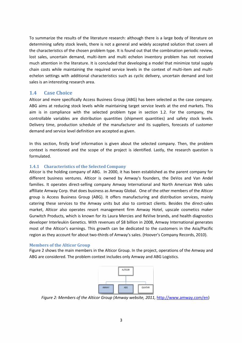
Members of the Alticor Group Figure 2 shows the main members in the Alticor Group. In the project, operations of the Amway and

ABG are considered. The problem context includes only Amway and ABG Logistics.

Figure 2: Members of the Alticor Group (Amway website, 2011, http://www.amway.com/en)

4

Characteristics of Amway Amway is a privately owned company in Ada, Michigan. In the late 1940s Richard DeVos and Jay Van

Andel became distributors for NUTRILITE, a California vitamin company that had pioneered network

sales. In 1958, when NUTRILITE's leadership was failing, DeVos and Van Andel decided to develop

their own product line. In 1959, they founded the American Way Association (later shortened to

Amway).Amway is now part of Alticor. It is one of the leading companies in direct selling e-

commerce and business to business services. Amway is mainly a sales company. It boasts more than

3 million independent consultants who sell its catalogue of more than 450 personal care, home care,

nutrition and commercial products. The products are sold in more than 80 countries and territories.

Its operations include research and development, product development and manufacturing, product

supply, logistics and core business functions (IT, marketing, etc). Two-thirds of the revenue comes

from Asia. China is an especially fertile market for the company. The product line consists of mainly

three groups: home care, personal care and home tech products. The top competitors of the

company are Avon, Clorox and Procter&Gamble. (Hoover's Company Records, 2010).

Characteristics of Access Business Group (ABG) Access Business Group is a production/supply chain company. It provides business to business

support services for product development, manufacturing, farming and logistic services. ABG’s major

clients consist of Alticor Corporation, Johnson & Johnson, Unilever and L’Oreal. The company

manages supply chains for Amway and online retailer Quixtar. The main activities of ABG include

control of European Central Warehouse which serves 25 countries with 21000 pallet positions. The

company executes picking and packing operations for 14 countries with 2300 locations. ABG

operates with an overall capacity of more than 1.7 million sq. ft. In addition to distribution, the

company provides contract manufacturing of cosmetics, nutritional supplements, and personal care

products for its affiliates and other clients. The company also offers printing and packaging services.

The top competitors of the company are AppTech, Menlo Worldwide and Procter &Gamble.

(Hoover's Company Records, 2010.

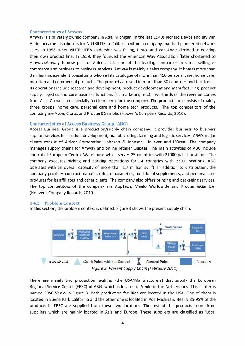
1.4.2 Problem Context In this section, the problem context is defined. Figure 3 shows the present supply chain.

Figure 3: Present Supply Chain (February 2011)

There are mainly two production facilities (the USA/Manufacturers) that supply the European

Regional Service Center (ERSC) of ABG, which is located in Venlo in the Netherlands. This center is

named ERSC Venlo in Figure 3. Both production facilities are located in the USA. One of them is

located in Buena Park California and the other one is located in Ada Michigan. Nearly 85-95% of the

products in ERSC are supplied from these two locations. The rest of the products come from

suppliers which are mainly located in Asia and Europe. These suppliers are classified as ‘Local

5

Sourced’, ‘European Sourced’ and ‘Far East Sourced’. The main reasons behind the idea of using

these suppliers are that for some cases, buying finished goods is less expensive compared to

producing in house.

ERSC Venlo provides logistics services for mainly seven sales points: Venlo pickline, Eastern European

Service Center (EESC-Hungary), Central European Service Center (CESC-Poland), Greece, Turkey,

Ukraine and finally Russia. It is important to mention that from the warehouses in the USA, there can

be also direct shipments to the sales points depending on the product type. The six sales points

excluding Venlo pickline are indicated by ‘Affiliates’ in Figure 3. Via Venlo pickline, ERSC Venlo

provides direct order fulfillment for Amway Business Owners (ABO’s) in fourteen countries. The

orders of these ABO’s are directly delivered by ERSC Venlo. In Figure 3, these customers are

indicated as ‘Customer WE’ (Western European countries). These Western European countries are

Belgium, the Netherlands, France, Germany, Austria, Switzerland, Spain, Portugal, Denmark,

Sweden, Norway, Finland, Italy and the UK. The rest of the end customers (ABO’s) for the affiliates

are named ‘Customer EE/RU’ (Eastern European countries and Russia). The sales point EESC is

located in Budapest. This sales point serves markets in Romania, Hungary, Croatia and Slovenia. The

CESC sales point which is located in Warsaw serves Poland, Czech Republic and Slovakia. Both EESC

and CESC have value added operations like labeling in their warehouses. The sales point in Russia

provides the direct order fulfillment to ABO’s only in this market. The sales points in Greece, Turkey

and Ukraine are not part of ABG. They are still entitled as Amway and they are independent in their

home operations.

1.4.3 Performance Measurement

ERSC Venlo has recently changed its focus from availability into availability with lower stock. This

change indicates that the company wants to lower stock levels in the overall supply chain while

meeting the service level targets.

The service level is defined in detail as follows: At the end of each day, it is checked whether there is

at least one item available on the shelf for a specific SKU or not. If there is, the stock is positive. The

rule works according to 0 or 1 principle. When there is no item available on the shelf at the end of a

day, it means that the item is not orderable even if there is no demand at all. The ratio of the total

number of days with positive stock over the total number of days in a year gives the service level

result for an SKU. It is important to indicate that the denominator also counts for the holidays; it is

not only the working days. Furthermore, there is no backorder system. If the product is not available

at the stock point when there is a customer who wants to order, lost sales are incurred.

Service Level on the item level:

This definition of the service level matches P3 service level definition in the literature (Silver et al.,

1998). It is defined as follows:

P3 (Specified Fraction of Time during Which Net Stock is Positive - Ready Rate): The ready rate is the

fraction of time during which the net stock is positive; that is, there is some stock on shelf.

6

1.4.4 Project Scope

The scope of the project is shown as in Figure 4.

Figure 4: Scope of the Project

The customers of ERSC Venlo include seven sales points (Venlo Pickline and other six affiliates). ERSC

Venlo aims at reaching target service levels at the affiliates while reducing costs for the entire supply

chain that starts with the production facilities in the USA and ends at the sales points. It is assumed

that the behaviors of the suppliers of the manufacturers and customers are given. Suppliers of the

manufacturers are out of scope mainly because of the complexity of data gathering and being USA

driven. Customers (ABO’s in the markets of affiliates) are also out of scope because they are

independent in their home operations. Local, European and Far East suppliers of ERSC Venlo are

kept out of scope mainly because of the low volumes they provide. Besides that, ERSC Venlo has

already developed a model for these suppliers. It is a simple Excel tool, which calculates costs

(purchasing cost, inventory carrying cost, order administration cost, freight cost, duty cost) for each

supplier candidate. The only performance measurement criterion is the costs involved. With the help

of this tool, the company can select the supplier with the lowest total cost. It is not possible to use

the same tool in this project, because in this project more parties are involved and not only the costs

but also service level targets are needed to be considered. Finally, the details of how forecast data is

calculated are not analyzed. It is used as input parameter. It is also be the case for lead time. How

routing is done or what combinations of transportation modes are used are also out of scope.

Since the aim of the project is to realize an integrated supply chain management, production

facilities that are located in the USA, ERSC Venlo and the other six sales points (‘Affiliates’) are

included in the scope of project. It should be noted that the project is on the higher level. Therefore,

the details of the production (how the products are produced and machine utilizations etc.) and

warehouse management at all locations are also out of scope.

1.4.5 Research Question

The potential problem to be checked is that the current inventory levels are higher than the

necessary levels which may have been resulting in high supply chain costs. This statement should

lead us to checking the possibility of reducing stock levels while satisfying the same target service

levels. There can be two possible reasons for high levels of inventory: either forecast data is not

7

accurate or inventory policy is not set correctly. In other words, it might be the case that the

demand data is overestimated most of the time and/or present inventory policy has some problems.

In this study, we do not deal with the forecast accuracy because it is given by Amway. Since it is not

controlled by ABG, we chose to continue with assessing the applied inventory policy and deal with

its problematic parts if any.

From the perspective of assessing present inventory policy, the potential problem might be either

the inventory policy parameters and rules that are used by ERSC Venlo are not set correctly or there

is the lack of coordination between the production facilities and ERSC Venlo. These potential

problems trigger the idea of analyzing the current supply chain and planning control mechanisms. It

also directs our interest to the question how overall supply chain costs can be minimized.

The main research question can be stated as ‘How to minimize total supply chain costs while

maintaining the required service levels?’. The service level definition is provided in section 1.4.3. The

required service levels are defined for each of the affiliates separately by the head office. The

relevant costs in our case include inventory carrying costs at the stock points and inventory carrying

costs for the items that are in-transit from one stock point to the next. Questions related to the

analysis of the present planning and control structures can be seen in Appendix I.

1.4.6 Deliverables

At the end of this project, the company expects to have a model implemented on software that can

be used to reach minimized total supply chain cost at the same time fulfilling the required service

level. First of all, the given supply chain is analyzed within the defined boundaries on the higher

level. After that, in the redesign phase alternative solutions that improve the performance of the

supply chain are proposed. With the help of this study, the planners of the company gain a tool that

makes life easier for them while setting the values for controllable variables with cost objective.

The rest of the report is organized as follows: in chapter 2, the present planning and control

structures are analyzed and the details of the pilot study are mentioned. In chapter 3, the

requirements of the inventory policy are presented. In chapter 4, the present inventory policy is

discussed with its pros and cons. In chapter 5, alternative solutions that deal with the weak points of

the present inventory policy are developed. In chapter 7, a simulation study is conducted in order to

gather the results of alternative solutions and compare them with the present system results. Before

going on with the details of simulation study in chapter 7, the simulation study is verified and

validated in chapter 6. In chapter 8, the content of the study is enriched with evaluating the

alternative policies under different scenarios. Finally, the study is concluded in chapter 9.

8

2. ANALYSIS

In this chapter, the detailed analysis of the supply chain structure in which ABG participates is

presented. First of all, the present planning and control structures are mentioned. Then, the demand

forecasting structures and the transportation structures are analyzed. Finally, the detailed

information is provided for the pilot study.

2.1 Present Planning and Control Structures In this chapter, each one of the stock points and decision points that are in the scope of the project

are analyzed in detail. The details of the cost calculations can be found in Appendix II. In our study,

the trade off is between service levels and inventory carrying costs. From that point of view, only

inventory carrying costs are found relevant.

There are two production facilities and two warehouses in the USA having the same structure. Figure

4 (in section 1.4.4) represents the structures for both of them. There are five main stock points in

the scope of the project. Stock point 5 refers to finished goods inventory. After stock point 5,

finished goods are sent to the warehouse in the USA (Stock point 4). After that ERSC Venlo decides

on the shipment quantities and gives the shipment orders to the warehouse in the USA. When the

finished goods arrive at ERSC Venlo, they are stored at stock point 3 for a relabeling process. The

relabeling process is not required for all of the items. After stock point 3, they are distributed to the

affiliates according to the planned parameters.

The concerned controllable parameters of the current supply chain are safety stock levels, shipment

volumes and shipment frequencies from Stock Point 4 to stock point 3, 2 and 1. Production schedule

of the manufacturer and its suppliers, forecasts of the customer (ABO’s) demand, lead times and

service level definition are accepted as given.

2.1.1. Affiliates-Stock Point 1 In the present planning and control structures, affiliates control the distribution of the products to

the end markets. However, it is ERSC Venlo’s responsibility to supply the necessary amount of

products to stock point 1. When the affiliates do not reach the target service levels, they ask ERSC

Venlo to make the necessary adjustments. For the six sales points (affiliates) excluding Venlo

pickline, ERSC Venlo keeps safety stock at stock point 1. The level of safety stocks is set by the

planners that are located in ERSC Venlo. When the inventory level at this point goes below the

safety stock level according to forecasted demand; the same planners place a shipment order from

stock point 4 to stock point 1 or from stock point 3 to stock point 1. The details of this process will be

discussed in section 2.1.2.

2.1.2. ERSC Venlo-Stock Points 1, 2 and 3, Control Points 1, 2, 3 and 4 In the present planning and control structures, ERSC Venlo decides mainly on: shipping volumes,

from stock point 4 to 3 and 1 and from stock point 2 to 1, and safety stock levels for the stock points

2 and 1. As mentioned earlier, stock point 2 includes safety stocks only for Venlo pickline. For the

other six sales points, safety stocks are kept at stock point 1. No safety stocks are kept at stock point

3.

9

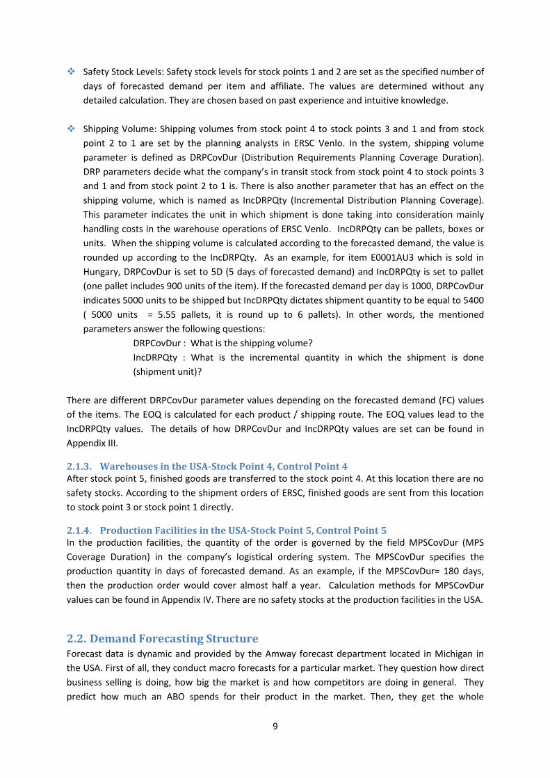
Safety Stock Levels: Safety stock levels for stock points 1 and 2 are set as the specified number of

days of forecasted demand per item and affiliate. The values are determined without any

detailed calculation. They are chosen based on past experience and intuitive knowledge.

Shipping Volume: Shipping volumes from stock point 4 to stock points 3 and 1 and from stock

point 2 to 1 are set by the planning analysts in ERSC Venlo. In the system, shipping volume

parameter is defined as DRPCovDur (Distribution Requirements Planning Coverage Duration).

DRP parameters decide what the company’s in transit stock from stock point 4 to stock points 3

and 1 and from stock point 2 to 1 is. There is also another parameter that has an effect on the

shipping volume, which is named as IncDRPQty (Incremental Distribution Planning Coverage).

This parameter indicates the unit in which shipment is done taking into consideration mainly

handling costs in the warehouse operations of ERSC Venlo. IncDRPQty can be pallets, boxes or

units. When the shipping volume is calculated according to the forecasted demand, the value is

rounded up according to the IncDRPQty. As an example, for item E0001AU3 which is sold in

Hungary, DRPCovDur is set to 5D (5 days of forecasted demand) and IncDRPQty is set to pallet

(one pallet includes 900 units of the item). If the forecasted demand per day is 1000, DRPCovDur

indicates 5000 units to be shipped but IncDRPQty dictates shipment quantity to be equal to 5400

( 5000 units = 5.55 pallets, it is round up to 6 pallets). In other words, the mentioned

parameters answer the following questions:

DRPCovDur : What is the shipping volume?

IncDRPQty : What is the incremental quantity in which the shipment is done

(shipment unit)?

There are different DRPCovDur parameter values depending on the forecasted demand (FC) values

of the items. The EOQ is calculated for each product / shipping route. The EOQ values lead to the

IncDRPQty values. The details of how DRPCovDur and IncDRPQty values are set can be found in

Appendix III.

2.1.3. Warehouses in the USA-Stock Point 4, Control Point 4 After stock point 5, finished goods are transferred to the stock point 4. At this location there are no

safety stocks. According to the shipment orders of ERSC, finished goods are sent from this location

to stock point 3 or stock point 1 directly.

2.1.4. Production Facilities in the USA-Stock Point 5, Control Point 5 In the production facilities, the quantity of the order is governed by the field MPSCovDur (MPS

Coverage Duration) in the company’s logistical ordering system. The MPSCovDur specifies the

production quantity in days of forecasted demand. As an example, if the MPSCovDur= 180 days,

then the production order would cover almost half a year. Calculation methods for MPSCovDur

values can be found in Appendix IV. There are no safety stocks at the production facilities in the USA.

2.2. Demand Forecasting Structure Forecast data is dynamic and provided by the Amway forecast department located in Michigan in

the USA. First of all, they conduct macro forecasts for a particular market. They question how direct

business selling is doing, how big the market is and how competitors are doing in general. They

predict how much an ABO spends for their product in the market. Then, they get the whole

10

estimated forecast for that particular market. After that, they distribute this estimated demand over

the items. Money spinning items have the priority. The forecasted demand data is provided on a

monthly basis by the forecasting department. Monthly forecast data is always in the system. At the

beginning of each year, forecast data is estimated for each month ahead of time. As time goes, it is

updated on the monthly level. As an example, at the beginning of the current month, forecast data

for two months ahead is estimated. As we get closer to that month, the forecast data in the system

is updated on the monthly level. The forecast department keeps track of the forecast data that is

estimated four months ahead, three months ahead etc. The important forecast data is the one that

is used for the shipment orders based on the lead time. As an example, if the lead time is 2 months

for shipping from stock point 4 to stock point 1, then the accuracy of the forecast data that is

estimated two months ahead is important.

2.3. Ordering Structure Regarding the production, there is sequencing of products. Products are produced approximately in

the cycles of 3 or 4 months. There is an opportunity window to put new orders in the production

schedule in the case of emergency. First of all, air transportation can be used for delivering products

from the USA to the Venlo warehouse. Secondly, the production frequency can be increased. Lastly,

there can be a blank version of products. Then, country specific labels can be added in Venlo.

2.4. Transportation Structure In this section transportation structure from the USA to the other stock points and from Venlo to the affiliates are mentioned. 2.4.1. Transportation from the USA The transportation from the USA has high variability since mostly sea transportation is used (nearly

100%). Air transportation is used when there are emergent situations since it is relatively expensive.

2.4.2. Transportation Modes from Venlo to Affiliates The transportation companies including Seacon Logistics that ABG group uses as 3PLs are

responsible just for delivery from Venlo to the affiliates. The routing is done by the transition

department of ABG. The transportation modes used are assumed to be fixed except for the

emergency cases and special products.

2.5. Pilot Study In this section, the detailed information is provided for the pilot study. First of all, the reasons of

item selection will be mentioned. Secondly, item specific details are presented. Finally, planning and

control structures for the selected item are mentioned.

2.5.1. Item Selection Criteria E0001 is the selected item for the pilot study. It is produced in Ada, USA. For the selected item, there

can be direct shipments to the sales points from production facilities depending on the end markets.

There are mainly three reasons for selecting this item: volumes, markets and availability of historical

data. This item is sold in high volumes and is saleable in all of the end markets. The company wants

to include most of the affiliates. Furthermore, it is not a revised item so there is historical data for

analyzing the demand pattern. It is checked whether the realized service levels and target service

levels are aligned for this item or not. Table 1 illustrates the service level values for the selected

11

item. As can be seen, the realized values are well above target values. These results also indicate

that the selected item is in compliance with the idea of the project. The idea of the project can be

summarized as follows: ‘The potential problem to be checked is that the current inventory levels are

higher than the necessary levels which results in high supply chain costs. This statement leads us to

the checking the possibility of reducing stock levels while keeping the same service level.’

Table 1: Realized P3 Service Levels and Target Values for item E0001

2.5.2. Present Planning and Control Structures for the Selected Items Figure 4 in section 1.4.4 illustrates the present planning and control structures for the selected item.

After stock point 4, item E0001 is shipped to ERSC Venlo for the end markets Venlo pickline, Turkey,

Greece and Ukraine (Route A). For the end markets Hungary, Poland and Russia, it is shipped directly

to the affiliates (Route B). There is the air transportation option for emergency cases. If it is seen

that the forecast value in the previous months are lower than the actual demand and/or the safety

stock level is less than the required level, the planning analyst can use the air transportation option

in order to cover demand during lead time. However, that option is not preferred for the selected

item due to its large unit size. Stock point 3 is included in the figure for relabeling process at ERSC

Venlo. It is important to mention that not all end market versions of E0001 are relabeled.

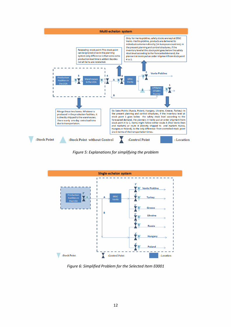
2.6. Problem Description It is important to mention that the focus is on the standard inventory flow in this project. In

everyday life, there might be manual flows. As an example, the shipment planner at ERSC Venlo

might contact the production facilities in order to fasten the production in the case of emergencies.

As another example, the planner might decide to transfer the finished goods from stock point 5 to

stock point 1 directly depending on the end market and volume to be shipped. However, these

actions are not defined in the company’s logistical ordering system software so they are ignored.

After the detailed analysis of the present planning and control structures in section 2.1, it is realized

that the problem can be simplified from a multi-echelon setting to a single echelon setting. Figure 5

illustrates how the problem can be simplified. It is important to note that this figure is not a key for

the redesign options. It is just an explicit transition of what the company is doing implicitly. From the

point of view of standard flow, whatever is produced in the production facilities, it is directly shipped

to the warehouses in the USA. The planner of the item sees whatever is at stock point 4 as available.

Stock point 3 indicates the relabeling step. Some of the items require relabeling at ERSC Venlo due

to language restrictions. However, it does not create a difference in the planning system structure. It

only requires adding some extra lead time in the system. Thus, it is ignored. Stock point 2 except for

ERSC Venlo pickline is not controlled. It is a transfer stock point. When these transitions are applied

the planning and control structures for item E0001 can be illustrated as in Figure 6.

12

Figure 5: Explanations for simplifying the problem

Figure 6: Simplified Problem for the Selected Item E0001

13

In the present system, production volume is controlled by the production facilities in the USA

according to the forecasted demand (Control Point 2 in Figure 6). Shipment quantity, how much to

ship from stock point 2 to 1 is controlled by the planners in ERSC Venlo (Control Point 1 in Figure 6).

As can be seen in Figure 6, the production facilities in the USA are considered as a black box at first.

However, the main aim of ERSC Venlo is to find the best possible solution for the two echelon case.

In this study first of all, alternative policies are developed for the single-echelon system. Then, with

the help of scenario analysis two echelon case is also considered.

14

3. REQUIREMENTS OF THE INVENTORY POLICY As figure 7 illustrates, in order to select an appropriate inventory policy there are two things to

consider: supply and demand patterns of the stock point. From that point of view, supply and

demand analysis for the selected item E0001 is conducted in this chapter. In the analysis, Russia is

selected as the end market since it is a large market and the impact of system changes will have

important effects in terms of volumes and profit margins. In the last section of this chapter, the

findings of the analysis are summarized in order to propose appropriate inventory policies that meet

the target service level and decrease the total inventory carrying costs in the following chapters.

Figure 7: Inputs for the Selection of the Inventory Policy

3.1. Detailed Demand Analysis for Item E0001 and End Market Russia In this section, demand pattern analysis for Russian version item E0001 is analyzed. First of all, actual

demand data is analyzed on monthly level. Then, daily demand pattern is analyzed. Finally,

forecasted demand data is analyzed.

3.1.1. Actual Demand Data Analysis It should be noted that meeting the assumption of stationary demand for selecting an appropriate

inventory policy is important. Silver et al. (1998) indicate that there are at least two circumstances

that can invalidate the assumption of stationary demand. First there may be a trend (linear or higher

order) in the underlying process. Second, there may be seasonality. Another point to consider for

selecting an appropriate inventory policy is the demand distribution. In this section, first of all, the

data is checked whether there exists a trend or not. Then, it is evaluated from the seasonality

perspective. After that we present the search for the probability distribution that fits the data in a

best way if there is any.

The Russian market is open since March 2005. We did not prefer to include the first year data in the

demand analysis since it might not be accurate due to some operational problems. Therefore, five

years of monthly demand data is used for the demand analysis starting from 2006 up to and

including 2010. We first focused on the monthly data because the daily demand data is highly

fluctuating, which makes hard to detect trend and seasonality if there is any.

In Appendix V, time series for the entire end markets that E0001 are sold are presented. Figure V.2

shows a time series that is based on the monthly Russian demand. It can be seen that there are

some peaks on the monthly level. According to the forecast department of the company, the biggest

reason behind the increases in sales is due to scheduled price increases. As an example, when the

company tell the distributors that they are going to have a price increase in March, sales will

increase significantly during February, or January.

In Appendix VI, the SPSS output for the trend analysis is presented. For that output, five years of

monthly data is used. Looking at the coefficients table reveals us that there is a significant increasing

15

trend since corresponding P value is less than 0.05. For a large market such as Russia, it is normal

that there is an increasing trend in the first years of the market.

There are also different graphical techniques for detecting seasonality. A time series pilot usually

shows seasonality if it is present. Using StatGraphs statistics software, a time series pilot is obtained

as can be seen in Appendix VII. From that plot, it is not easy to detect a seasonal demand pattern.

Three tests have been run to determine whether or not two years of monthly data is a random

sequence of numbers. A time series of random numbers is often called white noise, since it contains

equal contributions at many frequencies. The first test counts the number of times the sequence

was above or below the median. The number of such runs equals 10, as compared to an expected

value of 13.0 if the sequence were random. Since the P-value for this test is greater than or equal to

0.05, we cannot reject the hypothesis that the series is random at the 95.0% or higher confidence

level. The second test is similar to the first test. It counts the number of times the sequence rose or

fell around the mean. The number of such runs equals 15, as compared to an expected value of

15.66 if the sequence were random. Since the P-value for this test is also greater than or equal to

0.05, we cannot reject the hypothesis that the series is random at the 95.0% or higher confidence

level. The third test is based on the sum of squares of the first 24 autocorrelation coefficients. Since

the P-value for this test is greater than or equal to 0.05, we cannot reject the hypothesis that the

series is random at the 95.0% or higher confidence level (All the explanations and rules of thumb are

provided by the StatGraphs Statistics package itself).

The last topic that is discussed in this section is the demand distribution. Since service level is

calculated on the daily level, daily demand data is analyzed. Since one year of data constitutes a

large sample, only 2009 data is used. Service level is not calculated based on the working days.

Therefore, holidays are also included with zero demand. Using the EasyFit statistical package, it was

only possible to fit the demand data to the Wakeby distribution with a 95% confidence level.

Figure 8 shows the run chart for the daily demand data in 2009. The same analysis is also conducted

for the other years. The analysis of 2009 data is only presented here since one year daily demand

data constitutes a large sample. On the vertical axis sales volumes in units are illustrated. It can be

seen that the data is highly variable. At the end of each month, there are peaks at the last two or

three days of the months. The ratio of these peak days’ demand over the total monthly demand is

calculated per each month. The calculated ratios can be seen in Appendix VIII. It is observed that the

peak days constitute on average 32 % of the sales of total month. Those peak days make it hard to

find a suitable distribution fit. According to the company, they see huge end-of-month-sales in

Amway business in general always. It’s because of the fact that ABO's like to qualify for a certain

month volume. It is important to note that the demand data in 2009 is decreasing in Figure 8.

However, a trend analysis for the years 2009 and 2010 does not give a significant decreasing trend

Therefore; the decreasing trend in this figure is neglectable.

16

Figure 8: Russian daily demand 2009

To sum up, it is not possible to assume that demand is stationary in this case. It is mainly because

demand data shows a significant increasing trend and includes many peaks.

3.1.2. Forecasted Demand Data Analysis In the current system, forecast data for each coming month is kept. As an example, in January 2009,

forecasted demand values for the rest of the year is recorded. Then, they are updated on the

monthly level as time goes. It is expected that 3 months ahead forecasts would be more accurate

than 4 months ahead and 2 months ahead forecasts would be more accurate than 3 months ahead

forecasts. However, it is observed that it is not always the case for the selected item. How

forecasted demand deviates from the actual demand can be seen in Appendix IX. When two month

ahead forecasts are compared with the actual demand, it is found that the difference between the

forecasted demand and the actual demand is on average 10% applying the MAPE method (The mean

absolute percentage error) (Silver et al., in section 4.6, 1998).

3.2. Detailed Supply Analysis for Item E0001 and End Market Russia In this section, actual transportation times from stock point 2 (USA) to stock point 1 (Russia) are

analyzed. The lead time in the company’s logistical ordering system software has mainly three

components: transportation time, possible waiting time and handling time.

Figure 9, shows the analysis of one year data for actual direct transportation times. From stock point

2 to stock point 1 port sea transportation is used. From port to the Russian warehouse trucks are

used. The most up to date available data is used for the analysis since there might be changes with

routes at some points. In this way, the present situation can be reflected better. The data includes

more than 900 data points. The average transportation times are found to be 37 days and standard

deviation is found to be 6.24. However, in the present planning system transportation times are

accepted as deterministic. Only one parameter value can be defined in the company’s planning

software. In the models that are developed in chapter 5, the lead time is also treated as

deterministic. Since everyday there is a container available from stock point 2 to stock point 1, there

is no possible waiting time for this route. It is indicated that if the monthly average shipping

frequency is more than 17, only 3 days are added to the average lead time for the handling time.

That makes average lead time from Stock point 2 to Stock Point 1, 40 days.

17

Figure 9: Actual Transportation Times from stock point 2 to stock point 1 (October 2009-October

2010)

As stated by Silver et al. (in section 7.10, 1998), in most of the inventory literature it is assumed that

replenishment lead time is known. It is also indicated that where the pattern of variability is known,

for example, seasonally varying lead times, there is no additional problem because the lead time at

any given calendar time is known and the safety stock (and reorder point) can be adjusted

accordingly. Figure 10 shows monthly average results. From the graph it can be seen that, lead time

is higher in the first three months of the year which is probably due to winter season and it is lower

during the other months. However, the company does not consider this pattern. In the system, there

is only one input parameter value entry for the lead time and they use the average lead time value

during the whole year. It means that most of the time during the year, they use a longer lead time

than necessary, which means keeping higher levels of inventory and incurring higher inventory

carrying costs.

Figure 10: Monthly Average Actual Transportation Times from stock point 2 to stock point 1 (October

2009-October 2010)

Appendix X shows the monthly average actual times and standard deviations. It should be noted that

variability within the months is also high. Since lead times are stochastic, order crossing occurs from

time to time. However, in our case lead time is assumed to be deterministic at the first step in

chapters 4-5 since the company’s planning system software is also based on that assumption. As a

second step, possible solutions that take into account variability in the lead time itself are discussed

in chapter 8.

3.3. Summary of the Findings In order to select and appropriate inventory policy, the analyses of demand and supply patterns are

conducted in this chapter.

18

It should be noted that in the inventory literature, most of the time the focus is on normally

distributed demand (or forecast errors). It is stated that the normal distribution often provides a

good empirical fit to the observed data. Furthermore, the impact of using other distributions is

usually quite small (Silver et al., 1998). Tyworth and O’Neill (1997) and Lau and Zaki (1982) show

that, while the errors in safety stock may be high when using the normal, the errors in total cost are

quite low. The rule of thumb that is given by Silver et al. (in section 7.7.14, 1998) is that if the ratio σL

(standard deviation of the demand) /xL (average of the demand) is greater than 0.5 one must,

consider a distribution other than the normal. However, as long as this ratio is less than 0.5, the

normal is probably an adequate approximation. But in our case the ratio equals to 1. Silver et al.

(1998) also indicate that if daily demand is not normal, the normal will generally be a good

approximation for lead time demand if the lead time is at least several days in duration. But still in

our case, it is not possible to fit the demand during lead time to normal distribution although the

lead time is approximately 40 days. It is also stated that if the demand distribution is skewed to the

right, or if the ratio is greater 0.5, use of the Gamma distribution should be considered (Silver et al.

in section 7.7.14, 1998). However, the data in our case does not fit to the Gamma distribution

looking at the goodness of fits test results provided by the statistical packages. The Poisson

distribution is also a candidate for slower moving items. However, in our case it is not possible to fit

the demand data to Poisson, either (Appendix XI).

As mentioned earlier in this chapter, Silver et al. (1998) indicate that there are at least two

circumstances that can invalidate the assumption of stationary demand. First there may be a trend

(linear or higher order) in the underlying process. Second, there may be seasonality. The monthly

demand data is used in order to assess whether there exists a trend and seasonality or not in section

3.1.1. It is concluded that the demand data shows a significant increasing trend so it is not possible

to assume that it is stationary.

Another point to consider for applicability of the inventory policies is the service level definition. It is

stated that under Poisson Demand, P3 measure is equivalent with the P2 measure. (Silver et al.,

1998). Schneider (1981) discusses the ready rate for different inventory systems. It is assumed that

demand is stationary and lead time is constant. It is also assumed that there is never more than one

order outstanding. In this study, it is mentioned that if the assumptions are not met, the numerical

difficulties are insurmountable. It is also indicated that P3 service level plays no role in the lost sales

case. However, one of the characteristics of our problem is that it is a lost sales context and the

other one is that demand is non-stationary. Therefore, it is not possible to use the methods that are

given in this study.

Since it is not possible to find an appropriate model in the literature for P3 service level definition in

a lost sales non-normal, non-stationary demand environment; case specific solutions are developed

and the results of them are compared via a simulation study in chapter 7. Since items are produced

in cycles and the demand pattern is non-stationary, it is found appropriate to use time based

periodic review inventory control policies such as (Rt, st, St) or (Rt,St). They can be applied to cases

with non-stationary demand patterns. Different solutions are developed in chapter 5. Their results in

terms of service levels and inventory carrying costs for the single-echelon case are computed with

the help of a simulation study in chapter 7. After that, the effects of applying the developed

solutions on the total supply chain are assessed with alternative scenarios in chapter 8.

19

4. SINGLE ECHELON - PRESENT INVENTORY POLICY In this chapter, the idea behind the present inventory policy is discussed. The definitions and the

assumptions for this policy can be seen in Appendix XII.

4.1. The Idea behind the Policy The input parameters for the present policy are as follows: safety stock level at stock point 1

(Russia), shipping volumes and frequencies (review period) from stock point 2 (USA) to stock point 1,

lead time from stock point 2 to stock point 1, product value ($) and carrying cost %. Figure 11 is an

example that is used in the company instructions in order to explain the planning logic. It illustrates

what the company thinks they are doing with respect to the planning. On the horizontal axis, time in

weeks is indicated whereas on the vertical axis the quantity in terms of the forecasted demand

values are shown. In the figure, the safety stock level (SSCovDur) is defined as 8 weeks of the

forecasted demand and the shipping volume (DRPCovDur) from stock point 2 to stock point 1 is

defined as 18 weeks of the forecasted demand. Lead time from stock point 2 to stock point 1 is the

door (stock point 2) to door (stock point 1) lead time. The defined lead time is 4 weeks. Thus, when it

is assumed that the actual sales are exactly the same with the forecasted demand, it is expected that

every 18 weeks the inventory level hits the safety stock level. There are systematic warnings in the

planning system to ship, which is indicated with a red arrow in Figure 11. The warning is for the

shipment decision from stock point 2 to stock point 1. These warnings depend on the defined values

for the lead times in the system. For the given example, on the 14th week the system warns the

shipment planner and an order shipment decision from stock point 2 to stock point 1 for the volume

of 18 weeks of forecasted demand is released.

Figure 11: Planning Logic Explanation Example

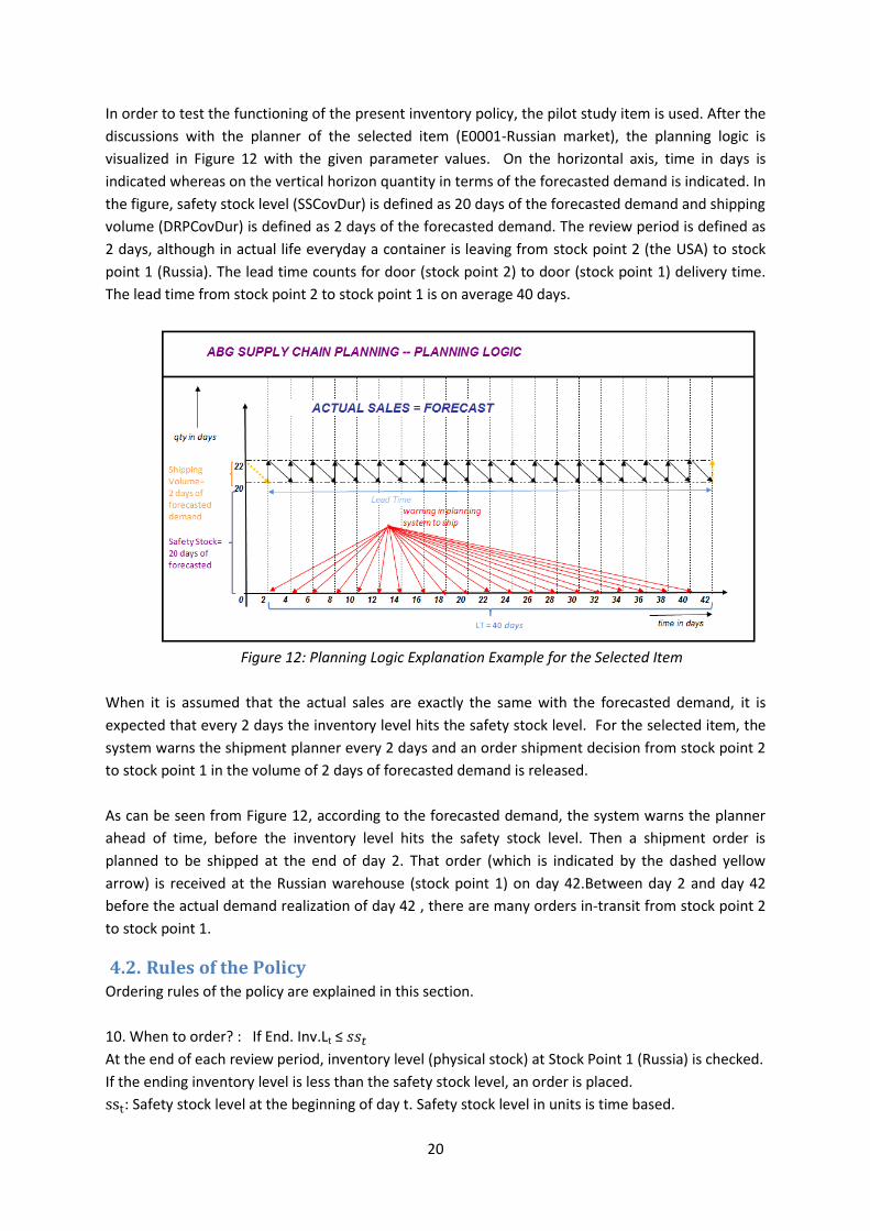
20

In order to test the functioning of the present inventory policy, the pilot study item is used. After the

discussions with the planner of the selected item (E0001-Russian market), the planning logic is

visualized in Figure 12 with the given parameter values. On the horizontal axis, time in days is

indicated whereas on the vertical horizon quantity in terms of the forecasted demand is indicated. In

the figure, safety stock level (SSCovDur) is defined as 20 days of the forecasted demand and shipping

volume (DRPCovDur) is defined as 2 days of the forecasted demand. The review period is defined as

2 days, although in actual life everyday a container is leaving from stock point 2 (the USA) to stock

point 1 (Russia). The lead time counts for door (stock point 2) to door (stock point 1) delivery time.

The lead time from stock point 2 to stock point 1 is on average 40 days.

Figure 12: Planning Logic Explanation Example for the Selected Item

When it is assumed that the actual sales are exactly the same with the forecasted demand, it is

expected that every 2 days the inventory level hits the safety stock level. For the selected item, the

system warns the shipment planner every 2 days and an order shipment decision from stock point 2

to stock point 1 in the volume of 2 days of forecasted demand is released.

As can be seen from Figure 12, according to the forecasted demand, the system warns the planner

ahead of time, before the inventory level hits the safety stock level. Then a shipment order is

planned to be shipped at the end of day 2. That order (which is indicated by the dashed yellow

arrow) is received at the Russian warehouse (stock point 1) on day 42.Between day 2 and day 42

before the actual demand realization of day 42 , there are many orders in-transit from stock point 2

to stock point 1.

4.2. Rules of the Policy Ordering rules of the policy are explained in this section.

10. When to order? : If End. Inv.Lt ≤

At the end of each review period, inventory level (physical stock) at Stock Point 1 (Russia) is checked.

If the ending inventory level is less than the safety stock level, an order is placed.

: Safety stock level at the beginning of day t. Safety stock level in units is time based.

21

At the beginning of each review period (day t), the safety stock level (SSCovDur) at stock

point 1 is the sum of the coming 20 days of the forecasted demand.

, where i=t,…,t+19

20. How much to order? : OQt+LT

At the end of day t, an order to be shipped from stock point 2 to stock point 1 is placed in the

amount of OQt+LT.

OQt: Order shipment quantity from stock point 2 to stock point 1 at the end of day t.

At the beginning of day t order quantity- OQt (DRPCovDur) is calculated as the sum of next coming 2

days of forecasted demand.

, where i=t,t+1

30. At the end of each day, if End. Inv.Lt >0, then the item is counted as orderable for that day.

40. At the end of each year, P3 service level is calculated.

4.3. Discussion of the Policy In order to test functioning of the present inventory policy, which is formally the logic used in the

company instructions a simulation study has been conducted. When the results of the simulation

study are analyzed, it is found that it is impossible to reach even target service levels by applying the

present inventory policy ordering rules. When the planner of the selected item is consulted about

the results of the simulation study for this policy, with the given parameter values (R=2,

,LT = 40 days ) it was found that rule 10 of the present inventory

policy is not applied for the selected item. Instead of applying it, every two days two days of

forecasted demand is shipped from stock point 2 to stock point 1. The results of the simulation

study for the true present inventory policy are discussed in chapter 6.

The advantage of present inventory policy is that shipping volumes change based on time. The

applied policy works for every type of demand pattern. Thus, there is no need to make the

assumption that demand is stationary. However, the main disadvantage is that, the system works

with deterministic input parameter values. It is also important to note that the review period can be

decreased without incurring any additional costs.

Another point to mention is that, although the target service level is 97% for the selected item, the

realized target levels are well above that target level as discussed in chapter 2. The reason behind

these high realized values might be that, the present inventory policy builds up inventory at stock

point 1 more than necessary. At the end of each review period, 2 days of forecasted demand is

shipped from stock point 2 to stock point 1 without checking the inventory position during lead time.

As Figure 12 signals, it might be the case that too much inventory is in transit to stock point 1 before

the actual realization of the demand. Then, the company spends much more money than necessary

in inventory carrying costs. In order to reduce inventory carrying costs while maintaining the target

service levels, two ordering rules are needed to be improved in the true present inventory policy:

when to order and how much to order rules. From that perspective four alternative inventory

policies are presented in chapter 5. Alternative 1 is exactly the same as present inventory policy

except for the review period value. Alternative 2 checks whether there is a need to order at the end

22

of each review period (day t) or not. If the inventory position is below safety stock level, then the

order is shipped from stock point 2 to stock point 1 in the amount of day t+LT’s forecasted demand

(LT: Lead time). This policy is expected to be better than the present one because it builds up fewer

inventories at stock point 1. Thus, it is expected that the inventory carrying costs will be less.

Alternative 3 applies the same rule as Alternative 2 policy for the question when to order but if it

orders, it orders the difference between forecasted demand for day t+LT and the expected inventory

available at the beginning of day t+LT. In this policy, it is also expected that the inventory carrying

cost will also be less. Alternative 4 is the same as Alternative 3. It is only a different version of

Alternative 3 from the practical implementation perspective. The impact of these new alternative

policies on the realized service level values might be different. In order to compare these four

policies in terms of safety stock levels, service levels and inventory carrying costs, simulation studies

have been conducted in Chapter 7.

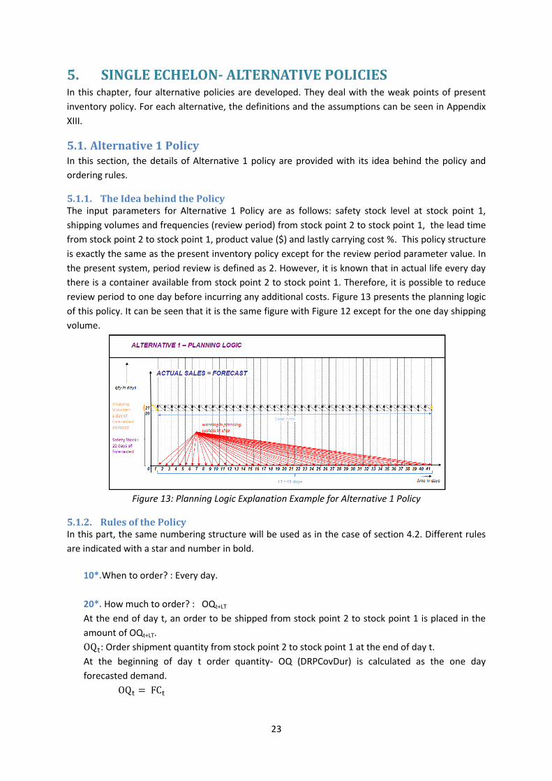
23

5. SINGLE ECHELON- ALTERNATIVE POLICIES In this chapter, four alternative policies are developed. They deal with the weak points of present

inventory policy. For each alternative, the definitions and the assumptions can be seen in Appendix

XIII.

5.1. Alternative 1 Policy In this section, the details of Alternative 1 policy are provided with its idea behind the policy and

ordering rules.

5.1.1. The Idea behind the Policy The input parameters for Alternative 1 Policy are as follows: safety stock level at stock point 1,

shipping volumes and frequencies (review period) from stock point 2 to stock point 1, the lead time

from stock point 2 to stock point 1, product value ($) and lastly carrying cost %. This policy structure

is exactly the same as the present inventory policy except for the review period parameter value. In

the present system, period review is defined as 2. However, it is known that in actual life every day

there is a container available from stock point 2 to stock point 1. Therefore, it is possible to reduce

review period to one day before incurring any additional costs. Figure 13 presents the planning logic

of this policy. It can be seen that it is the same figure with Figure 12 except for the one day shipping

volume.

Figure 13: Planning Logic Explanation Example for Alternative 1 Policy

5.1.2. Rules of the Policy In this part, the same numbering structure will be used as in the case of section 4.2. Different rules

are indicated with a star and number in bold.

10*.When to order? : Every day.

20*. How much to order? : OQt+LT

At the end of day t, an order to be shipped from stock point 2 to stock point 1 is placed in the

amount of OQt+LT.

: Order shipment quantity from stock point 2 to stock point 1 at the end of day t.

At the beginning of day t order quantity- OQ (DRPCovDur) is calculated as the one day

forecasted demand.

24

30. At the end of each day, if End. Inv.Lt >0, then the item is counted as orderable for that day.

End. Inv.Lt : Ending inventory level at stock point 1 at the end of day t.

40. At the end of each year, P3 service level is calculated.

5.2. Alternative 2 Policy In this section, the details of Alternative 2 policy are provided with its idea behind the policy and

ordering rules.

5.2.1. The Idea behind the Policy The input parameters in this alternative are the same as in Alternative 1 policy. As mentioned in

chapter 4, in the present structure, every two days there is a shipment from stock point 2 to stock

point 1. High values of realized service level indicate that the company is building up inventory more

than necessary. In order to reduce the inventory carrying costs, there is a need to check the

inventory position level before placing a shipment order. In this policy, instead of placing a shipment

order at the end of review period directly, first it is checked whether it is necessary to place an order

or not at the end of day t. If the inventory position is greater than safety stock level plus the

forecasted demand during lead time then nothing is done. Otherwise, an order is placed in the

volume of t+LT day forecasted demand (LT: Lead time). Apart from adding this checking mechanism,

the inventory policy stays the same as alternative 1 policy.

5.2.2. Rules of the Policy In this part, the same numbering structure will be used as in the case of section 4.2. Different rules

are indicated with a star and number in bold.

10*.When to order? : IPt < st .

At the end of each review period, if inventory position (IPt) is found to be more than st’ no order

is placed. If it is less than st,, then an order is placed.

IPt : Inventory position at the end of day t before placing an order.

sst : Safety stock level at the beginning of day t.

st : Threshold value for the ordering rule.

st= sst+ (safety stock level on day t + sum of the daily forecasted demand during the average lead time) , where i=t+1, …. i=t+LT

20*. How much to order? : OQt+LT

At the end of day t, an order to be shipped from stock point 2 to stock point 1 is placed in the

amount of OQt+LT.

: At the beginning of day t order quantity- OQ (DRPCovDur) equals to the daily forecasted

demand for that day.

30. At the end of each day, if End. Inv.Lt >0, then the item is counted as orderable for that day.

40. At the end of each year, P3 service level is calculated.

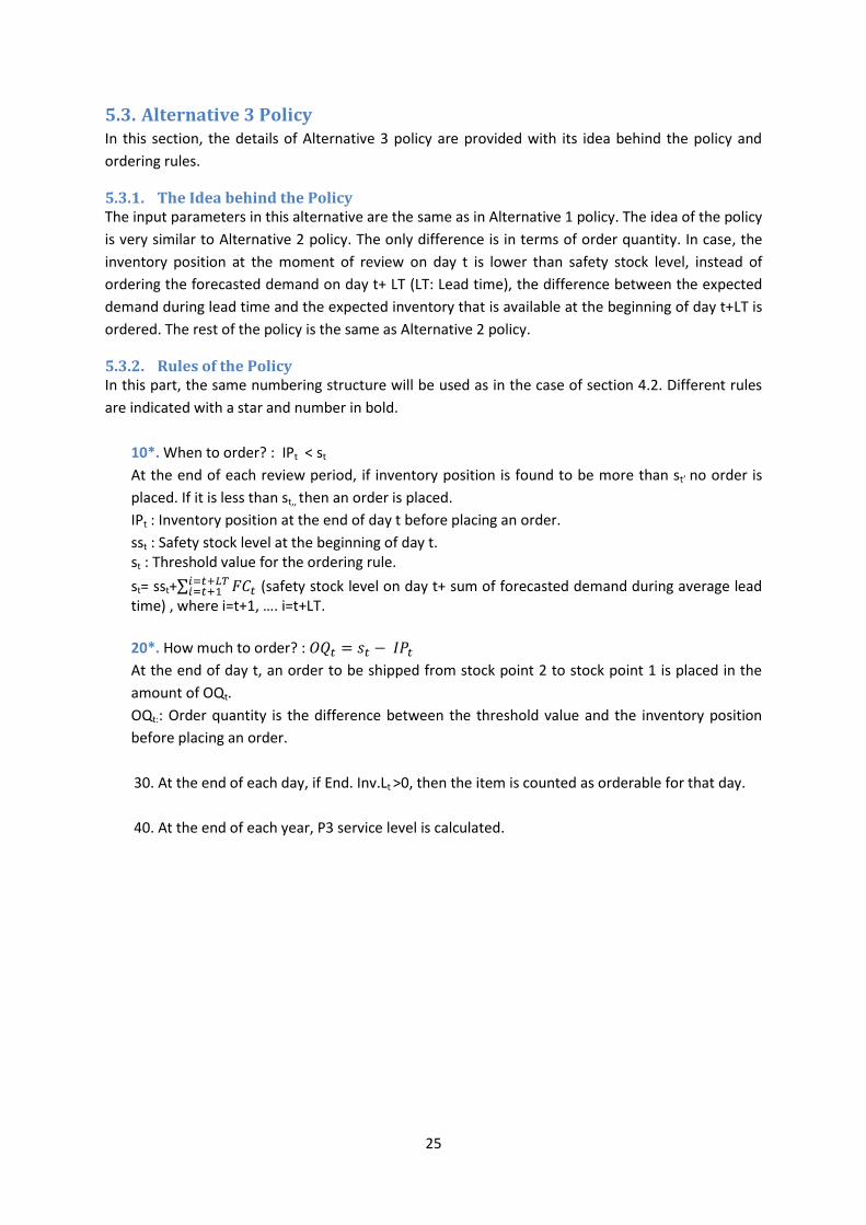
25

5.3. Alternative 3 Policy In this section, the details of Alternative 3 policy are provided with its idea behind the policy and

ordering rules.

5.3.1. The Idea behind the Policy The input parameters in this alternative are the same as in Alternative 1 policy. The idea of the policy

is very similar to Alternative 2 policy. The only difference is in terms of order quantity. In case, the

inventory position at the moment of review on day t is lower than safety stock level, instead of

ordering the forecasted demand on day t+ LT (LT: Lead time), the difference between the expected

demand during lead time and the expected inventory that is available at the beginning of day t+LT is

ordered. The rest of the policy is the same as Alternative 2 policy.

5.3.2. Rules of the Policy In this part, the same numbering structure will be used as in the case of section 4.2. Different rules

are indicated with a star and number in bold.

10*. When to order? : IPt < st

At the end of each review period, if inventory position is found to be more than st’ no order is

placed. If it is less than st,, then an order is placed.

IPt : Inventory position at the end of day t before placing an order.

sst : Safety stock level at the beginning of day t. st : Threshold value for the ordering rule.

st= sst+ (safety stock level on day t+ sum of forecasted demand during average lead time) , where i=t+1, …. i=t+LT.

20*. How much to order? :

At the end of day t, an order to be shipped from stock point 2 to stock point 1 is placed in the

amount of OQt.

OQt:: Order quantity is the difference between the threshold value and the inventory position

before placing an order.

30. At the end of each day, if End. Inv.Lt >0, then the item is counted as orderable for that day.

40. At the end of each year, P3 service level is calculated.

26

5.4. Alternative 4 Policy In this section, the details of Alternative 4 policy are provided with its idea behind the policy and

ordering rules.

5.4.1. The Idea behind the Policy The only different input parameter in this alternative is the order up to level at stock point 1. The

main difference is that, in this policy safety stock level is assumed to be zero and an order up to level

is defined. At the end of each review period, it is checked whether it is necessary to place an order or

not at the end of day t. If the inventory position is greater than the order up to level, then nothing is

done. Otherwise, an order is placed as the difference between order up to level and inventory

position.

5.4.2. Rules of the Policy In this part, the same numbering structure will be used as in the case of section 4.2. Different rules

are indicated with a star and number in bold.

10*. When to order? : IPt < St

At the end of each review period (day t), if the inventory position is found to be more than St no

order is placed. If it is less than St, then an order is placed.

IPt : Inventory position at the end of day t before placing an order.

St : Order up to level at the beginning of day t

20*. How much to order? : OQt = St- IPt

At the end of day t, an order to be shipped from stock point 2 to stock point 1 is placed in the

amount of OQt..

OQt:: Order quantity is the difference between the order up to level and the inventory position

before placing an order.

30. At the end of each day, if End. Inv.Lt >0, then the item is counted as orderable for that day.

40. At the end of each year, P3 service level is calculated.

5.5. Discussion of the Alternative Policies The only difference of alternative 1 policy from present inventory policy is that the review period is

decreased. As the review period decreases from 2 to 1, it is expected that total inventory carrying

cost at stock point 1 will also decrease. There will be no additional costs since everyday there is a

container leaving from stock point 2 to stock point 1. Therefore, it will be more advantageous to

apply this policy compared to present policy. On the other hand, alternative 1 policy does not

improve the ordering rules of present inventory policy. From that point of view, it is expected that

the realized service levels will not be aligned with target service levels.

The rest of the alternatives that are developed in this chapter also reduce the review period.

Furthermore, they aim at aligning the realized service levels with the target values. Alternative 2

policy checks inventory position before placing an order. It is expected that inventory carrying costs

will be less than the present policy. The main advantage of this policy over the present system is

that, it prevents the company from building high levels of inventory at stock point 1. However, it still

27

does not check how much to order depending on the available inventory position. It just orders one

day forecasted demand.

In order to see what happens if a similar checking mechanism is applied not only to ‘when to order?’

question but also to ‘how much to order?’ question; Alternative 3 policy is developed. In this policy,

instead of placing an order in the volume of one day forecasted demand, the difference between the

threshold value and inventory position is placed. With the help of this policy, order quantity

becomes more dependent on time. Taking into consideration service level results, the accuracy of

this policy over the years with variable demand patterns might be higher compared to Alternative 2

since shipment volume also depends on the difference between the ordering threshold value and

inventory position.

It is expected that the results of Alternative 3 and Alternative 4 in terms of inventory holding costs

and service levels will be the same. The only difference is in terms of number of parameters to be

controlled. Alternative 4 uses less parameter since safety stock level is set to zero. Therefore, these

two policies are different only from the perspective of implementing them into the company

logistical ordering system software. However, since the company is familiar with working safety

stock levels, Alternative 3 might still be more tempting for them.

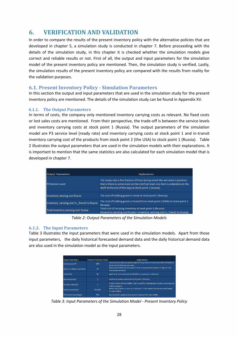
28

6. VERIFICATION AND VALIDATION In order to compare the results of the present inventory policy with the alternative policies that are

developed in chapter 5, a simulation study is conducted in chapter 7. Before proceeding with the

details of the simulation study, in this chapter it is checked whether the simulation models give

correct and reliable results or not. First of all, the output and input parameters for the simulation

model of the present inventory policy are mentioned. Then, the simulation study is verified. Lastly,

the simulation results of the present inventory policy are compared with the results from reality for

the validation purposes.

6.1. Present Inventory Policy - Simulation Parameters In this section the output and input parameters that are used in the simulation study for the present

inventory policy are mentioned. The details of the simulation study can be found in Appendix XV.

6.1.1. The Output Parameters In terms of costs, the company only mentioned inventory carrying costs as relevant. No fixed costs

or lost sales costs are mentioned. From their perspective, the trade-off is between the service levels

and inventory carrying costs at stock point 1 (Russia). The output parameters of the simulation

model are P3 service level (ready rate) and inventory carrying costs at stock point 1 and in-transit

inventory carrying cost of the products from stock point 2 (the USA) to stock point 1 (Russia). Table

2 illustrates the output parameters that are used in the simulation models with their explanations. It

is important to mention that the same statistics are also calculated for each simulation model that is

developed in chapter 7.

Table 2: Output Parameters of the Simulation Models

6.1.2. The Input Parameters Table 3 illustrates the input parameters that were used in the simulation models. Apart from those

input parameters, the daily historical forecasted demand data and the daily historical demand data

are also used in the simulation model as the input parameters.

Table 3: Input Parameters of the Simulation Model - Present Inventory Policy

29

6.2. The Verification of the Simulation Models Verification is necessary to determine whether a conceptual model is correctly represented by the

simulation software or not (Law and Kelton, 1991). Verification is the process of ensuring that the

simulation model behaves in the way it was intended according to the modeling assumptions made.

In other words, it is known as debugging the model. At this step, it is checked whether the model is

performing as designed. This step consists of probing the extreme regions of the input parameters,

ensuring that the right things happen with “obvious” input, and walking through the logic with the

ones who are familiar with the system (Kelton et. al., 2003).

Simple models can be easily verified. Verification becomes very important for larger models. It is

because there can be many different simultaneous activities occurring that may result in interactions

that were never intended. The simulation models are needed to be tested in order to find the

offending interactions and simple modeling mistakes. Kelton et. al. (2003) suggests trying different

input values and correcting found problems as a first step. The aim is to create a wide variety of

different situations where the model logic might just fail. The second step is to stand back and to

visualize different types of scenarios. The idea is to replicate projected scenarios as best as possible

and see if the model still performs adequately and the results make sense.

To summarize, with the help of verification step, the answer to the question “Did we do the things

right?” is chased after. In this chapter, we present how we verified our simulation models. For the

first step of the verification as suggested by Kelton et. al. (2003), we simply start applying the

consistency checks for the outputs of simulation models. We try different input values and check

whether the results are gained as expected. The flow of the entities and accuracy of the decisions

are tested for all the decision rules that are defined in the Chapters 4-5. After that we continue with

sensitivity analysis for the second step of the verification.

6.2.1. The Consistency Check for the Outputs of Simulation Models We firstly started with a model for the representation of the present planning and control

structures. Then, we added some details and changed the formulas for the replenishment decisions

in order to come up with the final versions of the alternative simulation models that have been

developed in Chapter 7. At every time an event occurred (placing an order, receiving an order or

occurrence of the demand) inventory positions and inventory levels are updated. After each

modification to the simulation models, randomly selected rows of the Excel sheets are debugged

and corrections are made if necessary. Per each day, ending inventory levels, ending inventory

positions and order quantities are analyzed using the graphical representations. The reasons of high

peaks are evaluated. In the end, it is ensured that the conceptual simulation models are correctly

translated and implemented in Excel worksheets. As an example for testing the accuracy of the flow

of entities, a randomly chosen 41- day period (namely, from day 731 to 772) is analyzed. It is

observed that the summation of the ‘Order Arrivals’ column gives the same result with the

summation of the ‘Forecasted Demand’ column. It can be concluded that the rule: ‘every two days

two days of forecasted demand is sent from stock point 2 (USA) to stock point 1 (Russia)’ works.

Furthermore, it can also be verified from Appendix XV.1 Table XV.I.3 that inventory balance

equations are satisfied and shipment order quantities are given and received as expected. The same

checks were also applied to the other policies that have been developed in this study.

30

6.2.2. Extreme value check As it is mentioned earlier in part 6.1, trying different input values and correcting found problems is

one of the first steps of the simulation model verification. The extreme value check was conducted

in order to see whether the models respond in a reasonable way to the extreme input values and

unlikely combination of levels of parameters. Before the sensitivity analysis, the models are checked

for the most basic situations with zero demand rate, zero forecasted demand rate, constant

forecasted demand, zero demand, constant demand=constant forecasted demand , constant

forecasted demand, constant demand greater than the forecasted demand, extreme forecasted

demand, extreme demand, and finally increased lead time. These are the most basic checks that

allow us to see whether there are some vital mistakes in the models or not. When the models pass

these checks, it is safer to continue with the sensitivity analysis part.

In this part of the report, the results of the original scenario (Present Inventory Policy) are

presented. The same checks are also applied to the simulation models that have been developed in

chapter 7 for the alternative policies. In all of the checks, the simulations models provided the

expected results and it was observed that the model logic did not fail. Thus, it can be concluded that

the simulation models seem to be working according to the intended logic and providing correct

results.

6.2.2.1. Zero Demand Rate When the forecasted demand stays the same but there is no demand at all, the system still sends

two days of forecasted demand since there is no inventory position checking in the present

inventory policy. Since demand is zero and the system still sends order quantities in the amount of

two days of forecasted demand from stock point 2 (the USA) to stock point 1 (Russia), high levels of

inventory is build up at stock point 1. Therefore, the average inventory carrying cost increases very

much. In transit stock cost is not affected since the total amount that is shipped just depends on the

forecasted demand and in this case we did not change the forecasted demand data. Since there is

always some positive inventory on hand at stock point 1, service levels reach 100%. In Appendix XIV

Table XIV.1 illustrates the results for this scenario. Alternatives 1-4 are also tested with the same

scenario. The results of Alternative 1 show the similar behavior with the present inventory system.

Since there is inventory position checks before placing an order in alternatives 2-4, the inventory

carrying cost does not go up and up continuously but still the service levels reach 100% as expected.

6.2.2.2. Zero Forecasted Demand Rate When the simulation models are tested with daily zero forecasted demand, there is no order

shipment decision and all the demand is lost. In Appendix XIV Table XIV.2 illustrates the results of

the present inventory policy for this scenario. The other alternatives are also checked with this

scenario and they give the expected results.

6.2.2.3. Constant Forecasted Demand, Zero Demand When the forecasted demand is assumed to be constant and equals to 8000 for each day and there

is zero demand, the present inventory policy builds up inventory in Russia (Stock Point 1). The

inventory carrying cost Russia increases in the period 2007-2010. Inventory carrying cost In_Transit

to Russia stays constant per each year. Service levels are always 100%. In Appendix XIV Table XIV.3

presents the results for this check. The other alternatives are also checked with this scenario. The

inventory position does not go below the level that triggers the order shipment decisions for

31

Alternative 2, 3 and 4 policies. No order is given as expected since these alternatives check the

inventory position before placing any order.

6.2.2.4. Constant Demand=Constant Forecasted Demand Another basic check is done with the constant demand and the forecasted demand in case they have

equal values. In Appendix XIV Table XIV.4 illustrates the results of the present inventory system.

When the forecasted demand and the actual demand are assumed to be constant and equal in the

case of the present inventory policy, service level reaches 50% on average. It is because in this

policy every 2 days 2 days of forecasted demand is shipped from stock point 2 (the USA) to stock

point 1(Russia). So, on the days with the order arrivals, ending inventory level is always positive but

for the rest it is always zero. For all the other alternatives, although all the demand is satisfied, P3

service level is always zero. It is because this level of definition becomes positive when there is at

least one item available at the end of the day. There is no inventory carrying cost. In-transit

inventory carrying cost is the same for all the years since every year the same amount of order

quantity is pulled from Stock Point 2 to Stock Point 1.

6.2.2.5. Extreme Forecasted Demand Another basic check is done with extreme forecasted demand values. The forecasted demand

amounts are set to 10 times larger than the original input data. The results of this scenario for the

present inventory system can be seen in Appendix XIV Table XIV.5.The present inventory policy

produces expected results (100 %) in terms of service levels. Inventory costs get higher and higher

from 2007 to 2010. It is clear that this policy is very much dependent on the forecasted demand and

it builds up inventory when the forecast data overestimates the actual demand data. Applying this

scenario to Alternative 2 and Alternative 3 policies makes them produce the expected outcomes

(100%) in terms of the service levels per each year. The inventory carrying costs also increases for

these alternatives but not as much as in the case of the present inventory policy.

6.2.2.6. Extreme Demand In this case, the demand amounts are set to 10 times larger than the original input data and the

forecasted demand values are stayed the same. It is expected that the target service levels will not

be reached and inventory carryings cost will be decreased for the present inventory policy and also

for the alternatives. In Appendix XIV Table XIV.6 illustrates the results for this scenario. Inventory

carrying costs are incurred only for the days that have zero demand and order arrivals at the same

time. Since order shipment volumes are based on the forecasted demand, on hand stock levels at

stock point 1 are never enough to satisfy the actual demand. Other models are also checked with

this scenario and they give the expected results.

6.2.2.7. Extreme Lead Time The last basic check is done with increased lead time. When the lead time value increases it is

expected that in_transit inventory carrying costs will increase. Service levels for the present

inventory policy might not be affected since it builds up inventory more than necessary anyway. On

the other hand, under this scenario, without changing the safety stock levels or order up to levels

service levels will be decreased for Alternatives 2-4. Table XIV.7 in Appendix XIV illustrates the

results for the present inventory system. The model gives the expected results for all of the

alternative policies.

32

6.3. Sensitivity Analysis In this part of the report, the effect of using different safety stock levels on the service levels and

inventory carrying costs are evaluated for Alternatives 2 and 3 policies. The results of Alternative 4

policy are not presented since it shows the same behavior with Alternative 3 policy.

Figure 14: P3 Service Levels and Inventory Carrying Costs for Different Safety Stock Days –Alternative 2 Figure 14 illustrates how Alternative 2 policy P3 service level and total inventory carrying costs

behave as the number of days for the safety stock level increases. This policy reaches the target

service level when the days for safety stock level are set to 6. At this point, total inventory carrying

cost becomes $63,546. As safety stock increases from 6 days of forecasted demand to 50 days of

forecasted demand, service level performance also increases. After that point, as the safety stock

days increases, the performance does not improve anymore. The same behavior also applies to total

inventory carrying costs. It is because Alternative 2 policy uses safety stock level for checking

whether to place an order or not. The order quantity does not depend on the safety stock level.

Therefore, increasing safety stock level up to a level (50 days in this case) increases ordering

frequency. When the maximum possible frequency is reached (everyday an order is placed), P3

service level and inventory carrying costs remain the same.

Figure 15: P3 Service Levels and Inventory Carrying Costs for Different Safety Stock Days -Alternative 3

Figure 15 illustrates how Alternative 3 policy P3 service level and total inventory carrying costs

behave as the number of days for the safety stock level increases. Alternative 3 policy also reaches

the target service level when the days for safety stock level is set to 6. When safety stock level is 6

days of forecasted demand, total inventory carrying cost becomes $66,030. As safety stock increases

from 6 days of forecasted demand to 50 days of forecasted demand, P3 service level hits 100% level.

Increasing safety stock days always increases total inventory carrying costs. It is because Alternative

3 inventory policy uses safety stock level not only for checking whether to place an order or not but

also for determining the order amount.

33

6.4. The Validation of the Simulation Models Validation is the process of ensuring that the model behaves the same as the real system. It

questions whether the input distributions match what is observed in the field or not. It also checks

whether the output performance measures from the model match up with those from reality or not.

While statistical tests can be carried out at this step, it is suggested that a good dose of common

sense is also valuable (Kelton et. al., 2003). In summary, validation step at the simulation studies try

to provide an answer to the question “Did we do the right thing?”.

Comparison of the outputs of the simulation with actual statistics is a step of validation. In

order to validate the simulation models, the results from the present inventory policy model

are compared with the results from the real system. It is not possible to compare the cost

results with the results from reality. It is because the company does not keep track of the

inventory carrying costs on the item level. All the costs are budgeted costs. So we are left

with only P3 service level statistics in order to check the validity of the simulation models.

Table 4 shows the output parameter results for the simulation model. In the first column of the

table, average results are presented.

Table 4: Simulation Results - Present Inventory Policy

The resulting total inventory carrying cost at stock point 1 on average was $82,877. It is important to

note that inventory carrying cost results are found to be very different from each other on the yearly

level. Especially the cost result in 2009 is very high compared to the other years. In order to find the

reason of that a detailed analysis has been conducted. Figure 16 includes the analysis of the

cumulative difference between the daily forecasted demand data and the daily actual demand data

in the period 2007-2010. The ending inventory levels are also illustrated for the same period. On the

vertical axis, volumes in units are presented whereas on the horizontal axis time in days of the years

are presented (365 = 1st year =2007, 720 = 2nd year = 2008 etc.). Since the present inventory policy

does not check the inventory position before placing an order, it is highly dependent on the given

forecasted demand data. As can be seen from the figure, this policy builds up inventory at stock

point 1. Between day 730 and day 1095 (Year 2009), the inventory goes up and up.

Figure 16: Analysis cost result differences on the yearly basis.

34

The planner of the selected item who is familiar with the system is also consulted about the logic

used in the conceptual model and the reasonableness of the results. We had several meetings for

the confirmation of the conceptual model. Input-output relationship is found reasonable when the

results of the simulation models are compared with the ones of the reality. Table 5 compares the

results of the present inventory policy simulation model with the reality.

Table 5: Comparing the Results of the Simulation Study with the Realized Values

With the given parameter values, it can be observed that average realized service level is higher than

the target service level (97%) at stock point 1 (Russia). The service level results are in compliance

with the TNA HIT’s report (the report that shows how many days the item is out of stock). It can be

seen that, the results exactly matches each other for years 2007 and 2009. When the planner of this

item is consulted about the results, it is indicated that in 2008 the selected item became TNA

(temporarily not available) mainly because of the bad weather conditions in the USA. The effect of

these conditions became apparent starting from September 2008. On contrary to that, the item does

not go TNA in that period in our simulation model. Since we are looking at the standard flow and

ignore the manual flows in the simulation, we cannot observe the impact of such extreme reality

cases in the results. Therefore, we incur a difference in terms of P3 service results for 2008. The

result for 2010 is also slightly less than the actual case. For that year the forecasted demand

underestimates the actual demand. In underestimated situations, the planners can fasten the

production with manual flows in real life. However, for simulation study it is not the case.

The second step in validation is interpretation of the behavior of the system in specific

situations, i.e. checking if the model’s behavior is parallel to real-life expectations (Law and

Kelton, 1991). For this purpose, safety stock levels are altered to observe the changes in the

resulting P3 service levels and inventory carrying costs for Alternative policies 1 and 2 in

section 6.3. It is observed that up to some level, increasing the safety stock level improves

service level results but also increases inventory carrying cost for all of the simulation

models. After some point, increasing safety stock level does not improve service level results

but still increases costs for the Alternative 3 and 4 policies. Thus, it can be concluded that

the system works as expected and it responds to the changes as it should be in real life.

To sum up, it can be said that the simulation models work correctly and the present inventory policy

simulation model is a representative of the actual system.

35

7. SIMULATION MODELS In order to compare the results of the alternative policies which were mentioned in chapter 5,

simulation models have been developed and implemented in Excel spreadsheets. First of all, the

output and input parameters of the simulation models are summarized. Then, the results of the

simulation models are presented for each alternative separately. As it is expected, applying

alternative 1 policy reduces the total inventory carrying cost but it does not reduce the gap between

the realized service levels and the target values. Alternative 2 and 3 policies align the service levels

with the target values and require reduced level of safety stock. Therefore, they result in less

inventory carrying costs. As it is expected, Alternative 4 policy gives the same results as Alternative 3

policy. The details of the results for each alternative are discussed at the end of this chapter.

In this simulation study, the developed models have time dimension and the state of the systems

changes at discrete points in time. Since P3 service level is calculated on the daily basis within the

company, the base time units in the simulation study is one day.

7.1. The Output Parameters The output parameters of the simulation models for alternative policies are P3 service level (ready

rate) and inventory carrying costs at stock point 1 and in-transit inventory carrying cost of the

products from stock point 2 (the USA) to stock point 1 (Russia). For each simulation model, the same

statistics are calculated. They are the same with the output parameters of the present inventory

policy, which are mentioned in section 6.1.1.

7.2. The Input Parameters Table 6 illustrates the input parameters that are used in the simulation models. For each alternative,

the input parameter values that are used in the analysis can be seen with their explanations. The

values for the alternative policies are indicated under the columns Alt. 1, Alt. 2, Alt.3, and Alt. 4. It is

important to mention that all of the simulation models can work with different input parameter

values. Apart from those input parameters, the daily historical forecasted demand data and the

daily historical demand data are also used in all of the simulation models as input parameters.

Table 6: Input Parameter Values of the Simulation Models

36

7.3. The General Structure of the Simulation Models The structure and details of the simulation models are presented in Appendix XV. The output and

input screens, the structure of the models and the formulas that were used for calculating the

output values are presented for each policy separately.

The sequence of events in each review period for all of the models developed can be listed as follows: At the beginning of the period: 10. Daily forecasted demand data is used as an input to the simulation model. It is used for deciding order shipment quantities from stock point 2 to stock point 1. 20. Beginning inventory levels and beginning inventory positions are calculated on the daily level. 30. Safety stock levels and order quantities are calculated for each day. Order Delivery: 40. Orders are received. 50. Inventory level is updated. It is increased in the amount with the receipt order. Demand Comes: 60. Demand that is directly satisfied from the shelf is calculated. 70. Inventory levels and inventory positions are updated. 80. In order to calculate P3 service level, days with positive ending inventory levels are counted. Period Ends: 100. An order is placed depending on the rules of the inventory policy. 110. Ending inventory levels, ending inventory positions and in_transit stock values are calculated.

7.4. The Results of the Simulation Models In this section, the results of the simulation models for each policy that is developed in chapter 5 are

presented.

7.4.1. The Results of the Simulation Model for Alternative 1 Table 7 shows the output parameter values for the simulation model. In the first column of the

table, average results are presented.

Table 7: Simulation Results for Alternative 1 Policy

Alternative 1 policy is an extension of the present inventory policy simply by reducing review period

from 2 days to 1 day. As table 7 illustrates, Alternative 1 policy results in high levels of P3 service

level since it has the same ordering rules with the present inventory policy. On the other hand, total

inventory carrying cost is decreased when it is compared to the present inventory policy. Inventory

carrying cost in 2009 is higher compared to the other years as in the case of present policy. The

reasoning of it is the same as Figure 16 illustrates in chapter 6.

37

7.4.2. The Results of the Simulation Model for Alternative 2 Table 8 shows the output results for the simulation model. In the first column of the table, average

results are presented. Safety stock level has been determined as 6 days of forecasted demand by

trial and error. When safety stock level is determined as 6 days of forecasted demand, the target

service level (97 %) is reached.

Table 8: Simulation Results for Alternative 2 Policy

With the help of this policy, the target P3 service level on average is achieved at stock point 1

(Russia).

Figure 17: Comparing the Results of the Present Inventory Policy (PIP) and Alternative 2 Policy

Figure 17 compares the results of this policy with the present inventory policy. The total costs are

reduced in the amount of $19,330 compared to the present inventory policy. It is important to

mention that yearly service level results are not very stable. In year 2009, target service level is not

reached. The main reason of it is that, inventory position is checked before placing an order but the

shipment volume still depends on one day forecasted demand in this policy. It might be the case

that, for some days, it is decided to place an order but order quantity might not be enough to meet

the demand. In order to show the time-based behavior of inventory position, safety stock level and

the ordering quantity of this policy, Figure XV.III.1 and Figure XV.III.2 are presented in Appendix XV.

7.4.3. The Results of the Simulation Model for Alternative 3 Table 9 shows the output results for the simulation model. In the first column of the table, average

results are presented. Safety stock level has been determined as 6 days of forecasted demand by

trial and error. When safety stock level is determined as 6 days of forecasted demand, the target

service level (97 %) is reached.

Table 9: Simulation Results for Alternative 3 Policy

38

Figure 18: Comparing the Results of Present Inventory Policy (PIP) and Alternative 3 Policy

Figure 18 compares the results of this policy with the present inventory system. With the help of this

policy, the target P3 service level is achieved at stock point 1 (Russia) and the total costs are also

reduced in the amount of $16,854 compared to the present inventory policy. It should be noted that

applying Alternative 2 policy is more beneficial in terms of costs than Alternative 3 policy. However,

Alternative 3 service level results across different years are more stable. In all of the years, the target

service level (97%) is reached. in Appendix XV, Figure XV.IV.1 and Figure XV.IV.2 show the time-

based behavior of inventory position, safety stock level and the ordering quantity. It can be observed

that ordering quantities of Alternative 3 policy are more variable compared to Alternative 2 policy.

7.4.4. The Results of the Simulation Model for Alternative 4 Table 10 shows the output parameter values for the simulation model for the years 2007-2010. In

the first column of the table, average results are presented. Order up to level has been determined

as 46 days of forecasted demand by trial and error. When the order up to level is set to 46 days of

forecasted demand, the target service level is reached (97 %).

Table 10: Simulation Results for Alternative 4 Policy

This policy gives the same results with Alternative 3 policy. The main difference between them is

that Alternative 4 policy works with less parameter compared to Alternative 3 policy. Safety stock

level is set to zero days of forecasted demand. This alternative is proposed just for the

implementation purposes. The company might prefer to work with this policy, which has less

parameter. So, Alternative 3 and Alternative 4 policies are different just from the practical

perspective (implementation in the company’s logistical ordering system software.)

7.5. Simulation Run Parameters Simulation models need three run parameters which are replication length, length of warm up

period, and number of replications. As it is mentioned before, it was not possible to fit the actual

demand data to any available probability distribution. Since it was not possible to generate demand

data based on a fitted probability distribution, the simulation runs were conducted with the

available historical demand data. Historical monthly demand data was available in period 2006-

2010. However, daily demand data was needed for the simulation and daily demand data was only

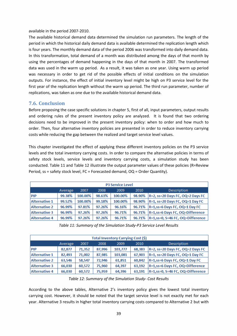
39

available in the period 2007-2010.

The available historical demand data determined the simulation run parameters. The length of the

period in which the historical daily demand data is available determined the replication length which

is four years. The monthly demand data of the period 2006 was transformed into daily demand data.

In this transformation, total demand of a month was distributed among the days of that month by

using the percentages of demand happening in the days of that month in 2007. The transformed

data was used in the warm up period. As a result, it was taken as one year. Using warm up period

was necessary in order to get rid of the possible effects of initial conditions on the simulation

outputs. For instance, the effect of initial inventory level might be high on P3 service level for the

first year of the replication length without the warm up period. The third run parameter, number of

replications, was taken as one due to the available historical demand data.

7.6. Conclusion Before proposing the case specific solutions in chapter 5, first of all, input parameters, output results

and ordering rules of the present inventory policy are analyzed. It is found that two ordering

decisions need to be improved in the present inventory policy: when to order and how much to

order. Then, four alternative inventory policies are presented in order to reduce inventory carrying

costs while reducing the gap between the realized and target service level values.

This chapter investigated the effect of applying these different inventory policies on the P3 service

levels and the total inventory carrying costs. In order to compare the alternative policies in terms of

safety stock levels, service levels and inventory carrying costs, a simulation study has been

conducted. Table 11 and Table 12 illustrate the output parameter values of these policies (R=Review

Period, ss = safety stock level, FC = Forecasted demand, OQ = Order Quantity).

Table 11: Summary of the Simulation Study-P3 Service Level Results

Table 12: Summary of the Simulation Study- Cost Results

According to the above tables, Alternative 2’s inventory policy gives the lowest total inventory

carrying cost. However, it should be noted that the target service level is not exactly met for each

year. Alternative 3 results in higher total inventory carrying costs compared to Alternative 2 but with

40

more stabilized service level results. Depending on the priority given either to P3 service levels or

inventory carrying costs, one of them can be selected for the single echelon case. Alternative 4 gives

the same results as Alternative 3. Alternative 4 sets safety stock level to zero, which enables it

working with less parameter. The difference between them is just from a practical point of view. The

choice between them depends on the implementation of the policies into the company’s logistical

ordering system software.

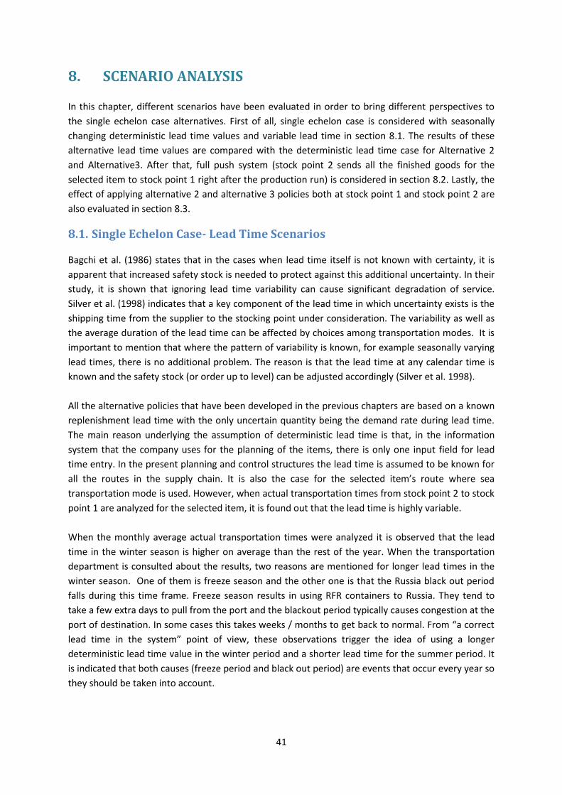
41

8. SCENARIO ANALYSIS In this chapter, different scenarios have been evaluated in order to bring different perspectives to

the single echelon case alternatives. First of all, single echelon case is considered with seasonally

changing deterministic lead time values and variable lead time in section 8.1. The results of these

alternative lead time values are compared with the deterministic lead time case for Alternative 2

and Alternative3. After that, full push system (stock point 2 sends all the finished goods for the

selected item to stock point 1 right after the production run) is considered in section 8.2. Lastly, the

effect of applying alternative 2 and alternative 3 policies both at stock point 1 and stock point 2 are

also evaluated in section 8.3.

8.1. Single Echelon Case- Lead Time Scenarios Bagchi et al. (1986) states that in the cases when lead time itself is not known with certainty, it is

apparent that increased safety stock is needed to protect against this additional uncertainty. In their

study, it is shown that ignoring lead time variability can cause significant degradation of service.

Silver et al. (1998) indicates that a key component of the lead time in which uncertainty exists is the

shipping time from the supplier to the stocking point under consideration. The variability as well as

the average duration of the lead time can be affected by choices among transportation modes. It is

important to mention that where the pattern of variability is known, for example seasonally varying

lead times, there is no additional problem. The reason is that the lead time at any calendar time is

known and the safety stock (or order up to level) can be adjusted accordingly (Silver et al. 1998).

All the alternative policies that have been developed in the previous chapters are based on a known

replenishment lead time with the only uncertain quantity being the demand rate during lead time.

The main reason underlying the assumption of deterministic lead time is that, in the information

system that the company uses for the planning of the items, there is only one input field for lead

time entry. In the present planning and control structures the lead time is assumed to be known for

all the routes in the supply chain. It is also the case for the selected item’s route where sea

transportation mode is used. However, when actual transportation times from stock point 2 to stock

point 1 are analyzed for the selected item, it is found out that the lead time is highly variable.

When the monthly average actual transportation times were analyzed it is observed that the lead

time in the winter season is higher on average than the rest of the year. When the transportation

department is consulted about the results, two reasons are mentioned for longer lead times in the

winter season. One of them is freeze season and the other one is that the Russia black out period

falls during this time frame. Freeze season results in using RFR containers to Russia. They tend to

take a few extra days to pull from the port and the blackout period typically causes congestion at the

port of destination. In some cases this takes weeks / months to get back to normal. From “a correct

lead time in the system” point of view, these observations trigger the idea of using a longer

deterministic lead time value in the winter period and a shorter lead time for the summer period. It

is indicated that both causes (freeze period and black out period) are events that occur every year so

they should be taken into account.

42

Taking into account the above mentioned points, Alternative 2 and Alternative 3 inventory policies

have been extended with variable lead times and also with seasonally changed known lead time

values. For the variable lead time scenario, actual transportation times are assumed to be normally

distributed (actual transportation times µ = 40,Ϭ = 6.23). For seasonally varying lead time different

values are entered per season (winter period lead time (4 months) = 42 days, summer period lead

time (8 months) = 38 days). With the help of extended simulations models (ordering rules do not

change but the receipt dates of orders are not known), the results are gained and they are presented

in Table 13 (Alternative 2 policy) and in Table 14 (Alternative 3 policy). It can be observed that the

variable lead times increase the safety stock level from 6 (deterministic lead time case) to 10 days of

the forecasted demand for both of the alternatives. When seasonality was taken into account, days

for the safety stock level decrease from 6 (deterministic lead time) to 5. It is observed that when the

days for safety stock increase or decrease, inventory carrying costs at stock point 1 also moves in the

same direction.

Table 13: Comparison of the Results of Lead Time Scenarios for Alternative 2 Policy

Table 14: Comparison of the Results of Lead Time Scenarios for Alternative 3 Policy

8.2. Two Echelon Case In the previous chapters, four different alternative inventory policies are developed. In this section,

the aim of the scenario analysis is to evaluate what happens to the inventory carrying costs at stock

point 2 when alternative 2 or alternative 3 is applied to stock point 2. First of all, the results of

applying the present inventory system rules to both of the stock points are evaluated. Secondly,

applying Alternative2 inventory policy to both stock points is evaluated in terms of total carrying

costs. Finally, applying Alternative 2 policy to stock point 2 and Alternative 3 policy to stock point 1 is

evaluated.

The input parameters of Stock Point 2 that are used in the simulation study for this scenario are

presented in Table 15. The input parameters for stock point 1 are stayed the same as in chapter 7.

The output parameters of the simulation study are presented in Table 16.

43

Table 15: Input Parameters Used for Stock Point 2

Table 16: Output Parameters Used for Two Echelon Case

8.2.1. The Results of Applying the Present Inventory Policy to Stock Point 2 & Stock Point 1

In the current system, the present inventory policy rules are also applied to stock point 2. Only the

input parameter values are different. At stock point 2, every fifteen days, fifteen days of forecasted

demand is produced. Then, ERSC Venlo decides on the shipment quantities from stock point 2 to

stock point 1. As mentioned earlier in chapter 5, in the present system every two days two days of

forecasted demand is sent from stock point 2 to stock point 1. Table 17 illustrates the results of this

scenario. P3 service level is higher than the target service level on average. The last line indicates the

total supply chain inventory carrying cost. It is the summation of inventory carrying cost at stock

point 2 (the USA), in-transit inventory carrying cost from stock point 2 to Stock Point 1 (Russia) and

inventory carrying cost at Stock Point 1. On average total supply chain cost is $97,287.

Table 17: Output Parameter Values - Present Inventory Policy

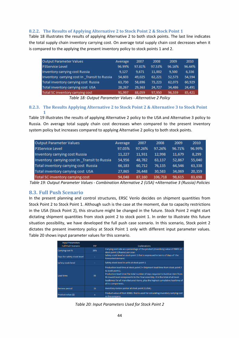
44

8.2.2. The Results of Applying Alternative 2 to Stock Point 2 & Stock Point 1 Table 18 illustrates the results of applying Alternative 2 to both stock points. The last line indicates

the total supply chain inventory carrying cost. On average total supply chain cost decreases when it

is compared to the applying the present inventory policy to stock points 1 and 2.

Table 18: Output Parameter Values - Alternative 2 Policy

8.2.3. The Results Applying Alternative 2 to Stock Point 2 & Alternative 3 to Stock Point 1

Table 19 illustrates the results of applying Alternative 2 policy to the USA and Alternative 3 policy to

Russia. On average total supply chain cost decreases when compared to the present inventory

system policy but increases compared to applying Alternative 2 policy to both stock points.

Table 19: Output Parameter Values - Combination Alternative 2 (USA) +Alternative 3 (Russia) Policies

8.3. Full Push Scenario In the present planning and control structures, ERSC Venlo decides on shipment quantities from

Stock Point 2 to Stock Point 1. Although such is the case at the moment, due to capacity restrictions

in the USA (Stock Point 2), this structure might be changed in the future. Stock Point 2 might start

dictating shipment quantities from stock point 2 to stock point 1. In order to illustrate this future

situation possibility, we have developed the full push case scenario. In this scenario, Stock point 2

dictates the present inventory policy at Stock Point 1 only with different input parameter values.

Table 20 shows input parameter values for this scenario.

Table 20: Input Parameters Used for Stock Point 2

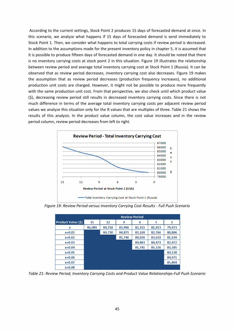
45

According to the current settings, Stock Point 2 produces 15 days of forecasted demand at once. In

this scenario, we analyze what happens if 15 days of forecasted demand is send immediately to

Stock Point 1. Then, we consider what happens to total carrying costs if review period is decreased.

In addition to the assumptions made for the present inventory policy in chapter 5, it is assumed that

it is possible to produce fifteen days of forecasted demand in one day. It should be noted that there

is no inventory carrying costs at stock point 2 in this situation. Figure 19 illustrates the relationship

between review period and average total inventory carrying cost at Stock Point 1 (Russia). It can be

observed that as review period decreases, inventory carrying cost also decreases. Figure 19 makes

the assumption that as review period decreases (production frequency increases), no additional

production unit costs are charged. However, it might not be possible to produce more frequently

with the same production unit cost. From that perspective, we also check until which product value

($), decreasing review period still results in decreased inventory carrying costs. Since there is not

much difference in terms of the average total inventory carrying costs per adjacent review period

values we analyze this situation only for the R values that are multiples of three. Table 21 shows the

results of this analysis. In the product value column, the cost value increases and in the review

period column, review period decreases from left to right.

Figure 19: Review Period versus Inventory Carrying Cost Results - Full Push Scenario

Table 21: Review Period, Inventory Carrying Costs and Product Value Relationships-Full Push Scenario

46

9. CONCLUSION AND FURTHER EXTENSIONS

This project is held in cooperation with ABG Supply Chain Management Department and aimed at

minimizing total supply chain costs while maintaining the required service levels. Our main research

question is stated as follows:

“How to minimize total supply chain costs while maintaining the required service levels?”

Total supply chain costs include inventory carrying costs at the stock points and inventory carrying

costs in-transit to end markets from the production facilities.

When we checked the realized (actual) service levels, we observed that they are well above the

target levels. The potential problem to be checked is that the current inventory levels are higher

than the necessary levels which may have been resulting in high supply chain costs. There were two

options to investigate for the cause of high levels of inventory: forecast accuracy and inventory

policy. In this study, we did not deal with the forecast accuracy because it is Amway driven. It is not

controlled by ABG. Therefore, we moved up the study into the inventory policy. We examined the

present inventory policy and deal with its problematic parts in order to align the realized service

levels with the target values.

In this study, we proposed inventory policy alternatives for an environment with lost sales, P3

service level requirement and non-stationary demand pattern. With the help of a simulation study,

our proposed alternative policies are shown to reduce not only the inventory carrying costs

compared to the original inventory policy used by the company but also the gap between the

realized service levels and the target values.

With the help of scenario analysis, the simulation models are extended in a way to integrate variable

lead times. It is found that safety stock levels need to be increased in order to cope with the

uncertainty of lead times and preserve target service levels. Secondly, the simulation models are

extended with deterministic lead times depending on the season. It is observed that when lead time

values are changing with the seasons and lead times per season are known safety stock level can be

decreased. So, it is better to use different values per season instead of using one value throughout

the year. It can be concluded that if the company finds a way to reduce its lead time variability

within the season, then there is room for further improvement in terms of carrying costs. As a third

scenario, we analyzed what happens if we apply Alternative 2 and Alternative 3 not only to Stock

Point 1 (Russia), but also to Stock Point 2 (the USA) at the same time. It is found that applying these

policies to both stock points reduces inventory carrying costs further. Finally, we checked what

happens if Stock Point 2 sends whatever produced directly to Russia. We found that as the

production frequency increases, inventory carrying costs at stock point 1 decreases. However, we

were aware of the fact that increasing the production frequency might mean that increased

production unit costs. From that perspective, we calculated breakeven points for the increased

production frequencies. Then, it became clear up to what unit cost it is still better to increase

production frequency.

It is important to note that our conclusions cannot be generalized to every case with the

characteristics of a single echelon, lost sales, non- stationary demand, variable lead times and P3

47

service level settings since they are drawn for the specific case under study. As a contribution to

academics, we provide an example to how to devise alternative policies for an inventory

environment in which it is not possible to model demand pattern with a probability distribution. We

also provide an example to how to compare proposed alternatives using the simulation. Since the

selected item has a non-stationary demand pattern, the developed models work with time based

ordering rules. The advantage of the developed models is that they can work with any demand and

supply pattern. Therefore, the company can use our models when making plans for other item and

end market combinations.

Due to time limitations, we applied our alternative policies only to one item and one end market

combination in this study. In order to increase the representativeness of this study, more products

are needed to be tested with them.

As another future research direction, handling costs can be incorporated into our study. We did not

consider handling costs in our models because the shipping volume unit is determined as one unit

for the selected item in the present system structure. For other items, shipping volume can be

dictated by pallet sizes. Our model can be extended to include pallet sizes for the shipments.

Another potential research can be analyzing the effect of reduced lead times on service levels and

total supply chain costs. In this study, we focused on the regular flows and we ignored the

emergency shipments. Besides, air shipment was not taken as an option for transportation due to

large size of the selected item. For different items, air shipment can also be considered and similar

models can be studied with the reduced lead times.

Our final and most important research suggestion is analyzing the effect of the improved forecast

accuracy on the service levels and total inventory carrying costs. In this study, we decided to assess

the present supply chain from the perspective of inventory policies since the forecast data is not

controlled by ABG. Even in that direction, we observed that the success of the inventory policies

highly depend on the forecast accuracy.

.

48

LIST OF ABBREVIATIONS ABG: Access Business Group

ABO: Amway Business Owners-individuals in the markets.

CESC: Central European Service Center

DRPCovDur: Distribution Requirements Planning Coverage Duration

EESC: Eastern European Service Center

ERSC: European Regional Service Center

FC: Forecasted Demand

IncDRPQty: Incremental Distribution Planning Coverage.

LT: Lead Time

MPSCovDur: MPS Coverage Duration

OQ: Order Quantity

PIP: Present Inventory Policy

ss: Safety Stock

SSCovDur: Safety Stock Coverage Duration

TNA: Temporarily Not Available

DEFINITIONS Customer: For the total supply chain, the end customers are the ABO’s in the country markets. ERSC

Venlo is responsible for meeting the service level requirements at the seven sales points. Thus, these

seven sales points (ABG Venlo (ERSC Venlo pickline), ABG Russia, ABG Hungary, ABG Poland, Amway

Turkey, Amway Greece and Amway Ukraine) constitute the customers in this project for ABG.

P3 Service Level (Ready Rate): The ready rate is the fraction of time during which the net stock is positive; that is there is some stock on the shelf (at least one item is orderable on the shelf) at stock point 1. Service Level on the item level:

49

LIST OF FIGURES Figure 1: Research design (based on Van Aken et al., 2007 and Van Strien, 1997)

Figure 2: Members of the Alticor Group (Amway website, 2011, http://www.amway.com/en)

Figure 3: Present Supply Chain (February 2011)

Figure 4: Scope of the Project

Figure 5: Explanations for simplifying the problem

Figure 6: Simplified Problem for the Selected Item E0001

Figure 7: Inputs for the Selection of the Inventory Policy

Figure 8: Russian daily demand 2009

Figure 9: Actual Transportation Times from stock point 2 to stock point 1 (October 2009- October

2010)

Figure 10: Monthly Average Actual Transportation Times from stock point 2 to stock point 1

(October 2009- October 2010)

Figure 11: Planning Logic Explanation Example

Figure 12: Planning Logic Explanation Example for the Selected Item

Figure 13: Planning Logic Explanation Example for Alternative 1 Policy

Figure 14: P3 Service Levels and Inventory Carrying Costs for Different Safety Stock Days - Alternative

2 Policy

Figure 15: P3 Service Levels and Inventory Carrying Costs for Different Safety Stock Days - Alternative

3 Policy

Figure 16: Analysis cost result differences on the yearly basis

Figure 17: Comparing the Results of Present Inventory Policy (PIP) and Alternative 2 Policy

Figure 18: Comparing the Results of Present Inventory Policy (PIP) and Alternative 3 Policy

Figure 19: Review Period versus Inventory Carrying Cost Results - Full Push Scenario

50

LIST OF TABLES Table 1: Realized P3 Service Levels and Target Values for item E0001

Table 2: Output Parameters of the Simulation Models

Table 3: Input Parameters of the Simulation Model for Present Inventory Policy

Table 4: Simulation Results for the present inventory policy Table 5: Comparing the Results of the Simulation Study with Realized Values

Table 6: Input Parameter Values of the Simulation Models

Table 7: Simulation Results for Alternative 1Policy Table 8: Simulation Results for Alternative 2 Policy Table 9: Simulation Results for Alternative 3 Policy Table 10: Simulation Results for Alternative 4 Policy Table 11: Summary of the Simulation Study P3 Service Level Results Table 12: Summary of the Simulation Study Cost Results

Table 13: Comparison of the Results of Lead Time Scenarios for Alternative 2 Policy

Table 14: Comparison of the Results of Lead Time Scenarios for Alternative 3 Policy

Table 15: Input Parameters Used for Stock Point 2

Table 16: Output Parameters Used for Two Echelon Case

Table 17: Output Parameter Values - Present Inventory Policy

Table 18: Output Parameter Values - Alternative 2 Policy Table 19: Output Parameter Values - Combination Alternative 2 (USA) +Alternative 3 (Russia) Policies

Table 20: Input Parameters Used for Stock Point 2

Table 21: Review Period, Inventory Carrying Costs and Product Value Relationships-Full Push Scenario

51

APPENDIX I: QUESTIONS RELATED TO THE PRESENT SUPPLY

CHAIN This Appendix presents questions related to the present planning and control mechanisms of the

present supply chain. They can help finding a solution for the problem of the company. The

answers of them are provided in chapter 2. Possible redesign options are also mentioned. Some of

them are evaluated in chapter 8.

Production facilities (USA/Manufacturers)

What kind of restrictions are there in the production?

Is there any production lead time uncertainty?

Which inventory policy is in use?

When do the plants produce each individual item?

In what amount are they produced?

Is it possible to change yearly production frequency of the products?

Is it possible to change the production schedule in the USA? How often can it be?

What is the cost of increasing the production frequencies?

What are the costs to be included at this step?

Are there any storage space restrictions for the finished goods inventory?

Transportation from USA to Venlo (L/T)

Is there any lead time uncertainty?

What is the distribution of the transportation time from USA to Venlo?

Who decides shipment quantities?

What are the transportation costs?

ERSC (Venlo)

Are there any storage space restrictions?

How much inventory is kept and where they are located?

Who decides and controls stocks?

Which inventory policy is in use?

Why are there high levels of stocks in the present policy?

For what items are there safety stocks?

How much safety stocks are kept?

What are the reasons behind the safety stocks?

What are the costs to be included at this step?

Transportation from Venlo to Affiliates (L/T)

Is there any lead time uncertainty?

What is the distribution of the transportation times from Venlo to Affiliates?

What are the transportation costs?

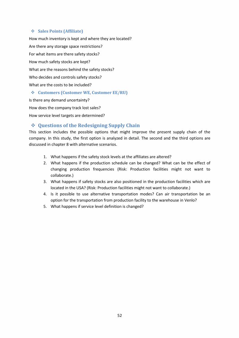
52

Sales Points (Affiliate)

How much inventory is kept and where they are located?

Are there any storage space restrictions?

For what items are there safety stocks?

How much safety stocks are kept?

What are the reasons behind the safety stocks?

Who decides and controls safety stocks?

What are the costs to be included?

Customers (Customer WE, Customer EE/RU)

Is there any demand uncertainty?

How does the company track lost sales?

How service level targets are determined?

Questions of the Redesigning Supply Chain This section includes the possible options that might improve the present supply chain of the

company. In this study, the first option is analyzed in detail. The second and the third options are

discussed in chapter 8 with alternative scenarios.

1. What happens if the safety stock levels at the affiliates are altered?

2. What happens if the production schedule can be changed? What can be the effect of

changing production frequencies (Risk: Production facilities might not want to

collaborate.)

3. What happens if safety stocks are also positioned in the production facilities which are

located in the USA? (Risk: Production facilities might not want to collaborate.)

4. Is it possible to use alternative transportation modes? Can air transportation be an

option for the transportation from production facility to the warehouse in Venlo?

5. What happens if service level definition is changed?

53

APPENDIX II: TOTAL SUPPLY CHAIN COST STRUCTURE

Affiliates-Stock Point 1 For this stock point, no cost data is provided except for the inventory carrying costs. Within the

company, carrying cost rates are defined as a percentage of the product (inventory) value of the

item per each stock point separately. Carrying costs are an estimate. They are not identified

separately on the income statement. Instead, carrying costs are usually buried in other categories

within the income statement, such as cost of sales and operating expenses (such as employee,

facilities/equipment, and freight/shipping expenses).

ERSC Venlo-Stock Points 2 and 3, Control Points 2,3 and 4 Total Cost for Venlo: Total Inventory Carrying Cost + Handling Cost + Ordering Cost+ Transportation Cost (For the route B). Total Inventory Carrying Cost

In order to calculate the total average inventory carrying cost, a percentage value is calculated

depending on the following cost components.

Total Inventory Carrying Cost excluding handling cost (Cost as % of inventory value) = Opportunity Cost ERSC Venlo + Occupancy Costs ERSC Venlo + Inventory Control ERSC Venlo + Non-saleable Inventory Cost ERSC Venlo

1) Opportunity cost percentage indicates what would be the benefits if the company invested

the money by taking an alternative action. Its value is Alticor’s current short term lease vs.

buy financing rate.

2) Occupancy cost includes costs such as rental costs, utilities, service costs (building, parking

lot maintenance) and extra handling requirements.

3) Inventory control cost includes the costs paid for cycle counting staff.

4) Non-saleable inventory cost is also part of the fixed costs. It includes scrapping costs,

handling costs for scrap and scrapping administration cost.

Handling Cost

Average Cost per LP (Licence Plate-move) in dollars ($)

On average it is assumed that a pallet has 2 LPs (One for loading and one for unloading). The

handling cost can be calculated as follows:

Average number of pallets*2*$ the cost of one movement per pallet

Transportation Cost

Over-labelling Cost

Warehouses in the USA-Stock Point 4, Control Point 4 Transportation Cost

Inventory Carrying Cost and Handling Cost

Production Facilities in the USA-Stock Point 5, Control Point 5 Transportation Cost

Inventory Carrying Cost

Handling Cost

Production Cost (For calculation of setup costs main components are: planning cost, quality

pull/retrieval material cost, administration cost and machine setup cost.

54

APPENDIX III: CALCULATION OF DRPCOVDUR AND

INCDRPQTY VALUES According to FC values, DRPCovDur values are set. As an example for setting DRPCovDur, if the

FC value of an item is more than 20 pallets per month, its DRPCovDur is set to 2 days. The rest

DRPCovDur settings can be seen below. There are not any particular reasons why ERSC Venlo

planners determined DRPCovDur values as they are.

FC > 20pallets / month DRPCovDur = 2 (Approximately every 2 days there is a

shipment)

FC > 1pallet / month DRPCovDur = 5 (Approximately every 5 days there is a

shipment)

FC <= 1pallet / month DRPCovDur = based on EOQ / FC per day (maximum

DRPCovDur = 56 days)

According to EOQ quantities incremental shipment quantities are set. As an example, if it is

found that the EOQ for an item is more than its pallet quantity, shipment is decided to be done

in multiples of pallets. The break points can be seen below and they are all based on intuitive

knowledge, too.

EOQ > 1 Pallet Quantity IncDRPQty = Pallet (Shipment is done in pallets)

EOQ > 0.75 * Tie Quantity IncDRPQty = Tie (Shipment is done in ties)

EOQ > 0.5 * Master Pack Quantity IncDRPQty = Master Pack (Shipment is done in

master packs)

EOQ > 0.25 * Mailer Quantity IncDRPQty = Mailer (Shipment is done in mailers)

EOQ < 0.25 *Mailer Quantity. IncDRPQty = Each (Shipment is done in eaches)

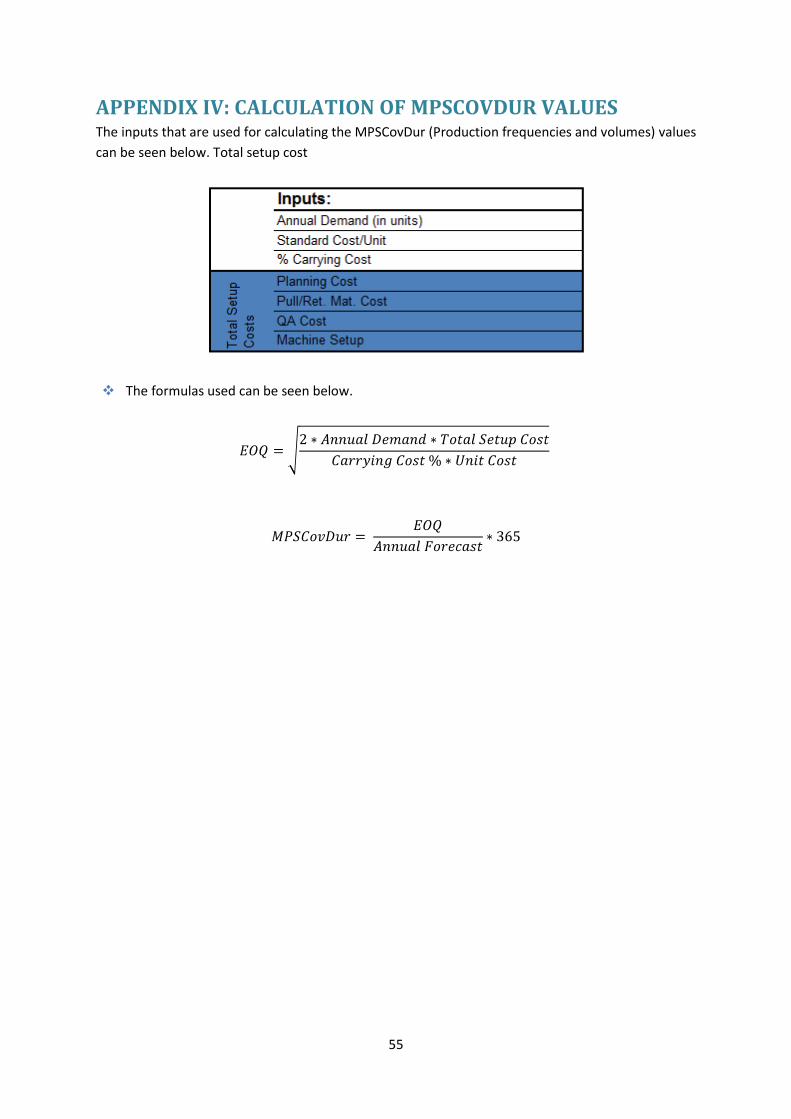
55

APPENDIX IV: CALCULATION OF MPSCOVDUR VALUES The inputs that are used for calculating the MPSCovDur (Production frequencies and volumes) values

can be seen below. Total setup cost

The formulas used can be seen below.

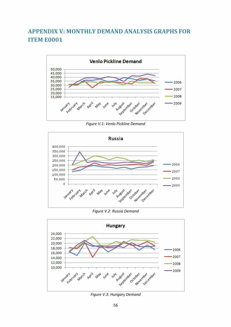
56

APPENDIX V: MONTHLY DEMAND ANALYSIS GRAPHS FOR

ITEM E0001

Figure V.1: Venlo Pickline Demand

Figure V.2: Russia Demand

Figure V.3: Hungary Demand

57

Figure V.4: Poland Demand

Figure V.5: Ukraine Demand

Figure V.6: Greece Demand

58

Figure V.7: Turkey Demand

59

APPENDIX VI: TREND ANALYSIS FOR ITEM E0001 AND END

MARKET RUSSIA

Determination of the Trend Line-Significant increasing trend for five years of data (2007-2010)

60

APPENDIX VII: SEASONALITY ANALYSIS FOR ITEM E0001 AND

END MARKET RUSSIA

Monthly Run Sequence Pilot for Item E0001 and End Market Russia

O n the X axis, time values are plotted starting at January 2008 and on the Y axis sales values are piloted.

Tests for Randomness for Item E0001 and End Market Russia (Period 2008-2009)

Tests for Randomness of Col_1 (1) Runs above and below median Median = 238812. Number of runs above and below median = 10 Expected number of runs = 13.0 Large sample test statistic z = 1.04356 P-value = 0.296688 (2) Runs up and down Number of runs up and down = 15 Expected number of runs = 15.6667 Large sample test statistic z = 0.0839181 P-value = 0.933116 (3) Box-Pierce Test Test based on first 8 autocorrelations Large sample test statistic = 1.9744 P-value = 0.981787

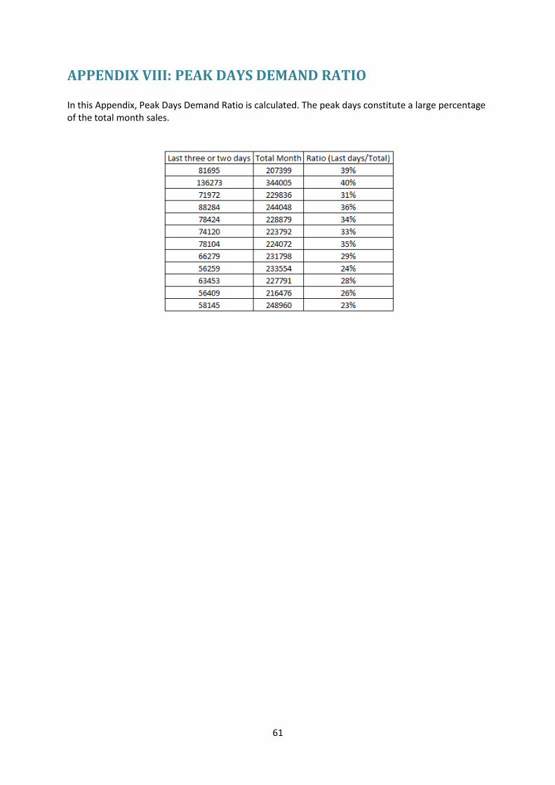
61

APPENDIX VIII: PEAK DAYS DEMAND RATIO In this Appendix, Peak Days Demand Ratio is calculated. The peak days constitute a large percentage of the total month sales.

62

APPENDIX IX: FORECASTED DEMAND DATA This Appendix illustrates the different periods ahead forecasted demand data and compares them

with the actual demand.

63

APPENDIX X: SUPPLY ANALYSIS FOR E0001 AND END

MARKET RUSSIA In this appendix, monthly transportation times from stock point 2 (the USA) to stock point 1 (Russia)

are analyzed. The monthly averages and standard deviations are calculated per each month.

Monthly Actual Transportation Analysis

Date Average

Standard

Deviation

okt-09 35 2,54

nov-09 34 3,62

dec-09 36 6,20

jan-10 40 5,18

feb-10 39 7,03

mrt-10 40 8,26

apr-10 38 7,66

mei-10 35 3,74

jun-10 36 5,25

jul-10 35 6,93

aug-10 34 4,08

sep-10 35 4,73

okt-10 35 4,85

64

APPENDIX XI: DEMAND DISTRIBUTION ANALYSIS FOR E0001

AND END MARKET RUSSIA In this Appendix, the goodness of test results for the distribution fitting are illustrated.

65

APPENDIX XII: PRESENT INVENTORY POLICY In this Appendix, the definitions and the assumptions of the present inventory policy are mentioned.

Appendix XII.I. Definitions of the Present Inventory Policy 10. Carrying cost %: Within the company, carrying cost rates are defined as a percentage of the product (inventory) value of the item per each stock point separately. 20. Dt : Actual demand data for the end market at day t. 30. End. Inv.Lt : Ending inventory level at stock point 1 at the end of day t. 40. FCm,m-2: Monthly forecasted demand data for the actual sales at the end market in month ‘m’ that is estimated in month ‘m-2’ ( 2 months ahead forecasted demand data was used in the analysis for the selected item since the lead time from stock point 2 to stock point 1 is 40 days. ) 50. FCt,m : Daily forecasted demand data that is obtained by dividing FCm,m-2 by the number of days in month m.

FCt,m=

60. Inventory carrying cost: Costs of holding goods in stock at stock point 1. In order to calculate the inventory carrying cost per year at stock point 1, daily ending inventory

levels are summed. Then, it is multiplied with the daily carrying cost percentage and the product

value.

70. In-transit inventory carrying cost: Cost of holding goods in transit from stock point 2 to stock point 1. In-transit inventory carrying cost from stock point 2 to stock point 1 is calculated as follows:

80. LT: Lead time (door to door) from stock point 2 to stock point 1 90. OQt: Order shipment quantity from stock point 2 to stock point 1 at the end of day t.

100. Product (inventory) value ($): Product value of the selected item that is used for calculating inventory carrying cost at stock point 1. 110. P3 service level: The ready rate is the fraction of time during which the net stock is positive; that is there is some stock on the shelf (at least one item is orderable on the shelf) at stock point 1. 120. R : Review period 130. sst : Safety stock level at the beginning of day t.

66

Appendix XII.II. Assumptions of the Present Inventory Policy

10. FCm,m-2 is assumed to be given.

20. In the actual every day operations, transportation lead time from stock point 2 to stock point

1 varies and order crossings might occur. However, in the system the lead time is assumed

to be deterministic and order crossings are ignored.

LT: 40 days

30. Review period is assumed to be 2 days.

R:2 days

40. An order that is placed on day t is received on day t+LT (t+40 days).

50. Carrying cost % at stock point 1 is assumed to be 20% of the product value of the item per

year. So if $100 worth of a stock keeping unit (SKU) in a year is carried, then $20 is paid for

carrying costs.

60. Product value of the selected item is given as x $.

70. At the beginning of each review period (time t), the safety stock level (SSCovDur) at stock

point 2 is calculated as the sum of the coming 20 days of the forecasted demand.

, where i=t,…t+19

80. At the beginning of day t order quantity- OQ (DRPCovDur) is calculated as the sum of next

coming 2 days of forecasted demand.

, where i=t,t+1

67

APPENDIX XIII: ALTERNATIVE POLICIES In this Appendix, first of all the definitions of the alternative policies are mentioned. After that the

assumptions that are common to all of the alternative policies are mentioned. Finally, alternative

policy specific assumptions are presented. The same numbering structure is used as in the case of

chapter Appendix XII. Different definitions and assumptions are indicated with a star and number in

bold.

Appendix XIII.I. Definitions of the Alternative Policies 10. Carrying cost %: Within the company, carrying cost rates are defined as a percentage of the product (inventory) value of the item per each stock point separately. 20. Dt : Actual demand data for the end market at day t. 30. End. Inv.Lt : Ending inventory level at stock point 1 at the end of day t. 40. FCm,m-2: Monthly forecasted demand data for the actual sales at the end market in month ‘m’ that is estimated in month ‘m-2’ ( 2 months ahead forecasted demand data was used in the analysis for the selected item since the lead time from stock point 2 to stock point 1 is 40 days. ) 50. FCt,m : Daily forecasted demand data that is obtained by dividing FCm,m-2 by the number of days in month m.

FCt,m=

60. Inventory carrying cost: Costs of holding goods in stock at stock point 1. In order to calculate the inventory carrying cost per year at stock point 1, daily ending inventory

levels are summed. Then, it is multiplied with the daily carrying cost percentage and the product

value.

70. In-transit inventory carrying cost: Cost of holding goods in transit from stock point 2 to stock point 1. In-transit inventory carrying cost from stock point 2 to stock point 1 is calculated as follows:

75.* IPt : Inventory position at the end of day t before placing an order. (It is used for Alternative 2,

3 and 4 Policies).

80. LT: Lead time (door to door) from stock point 2 to stock point 1 90. OQt: Order shipment quantity from stock point 2 to stock point 1 at the end of day t. 100. Product (inventory) value ($): Product value of the selected item that is used for calculating inventory carrying cost at stock point 1.

68

110. P3 service level: The ready rate is the fraction of time during which the net stock is positive; that is there is some stock on the shelf (at least one item is orderable on the shelf) at stock point 1. 120. R: Review period 125.* ssc: Constant safety stock level in units that meets the service level criterion. The value of it is found by trial and error (It is used for only Alternative 2 Policy & Alternative 3 Policy). 130. sst : Safety stock level at the beginning of day t. 140.* st : Threshold value for the ordering rule (It is used for only Alternative 2 Policy & Alternative 3 Policy). 150.* Sc : Constant safety stock level in units that meets the service level criterion. The value of it is found by trial and error (It is used only for Alternative 4 Policy) 160.* St : Order up to level at the beginning of day t (It is used only for Alternative 4 Policy).

Appendix XIII.II. Assumptions of the Alternative Policies In this Appendix, first the common assumptions of the Alternative Policies are presented. Then, the

alternative specific assumptions are presented separately.

10. FCm,m-2 is assumed to be given.

20. In the actual every day operations, transportation lead time from stock point 2 to stock point

1 varies and order crossings might occur. However, in the system the lead time is assumed

to be deterministic and order crossings are ignored.

LT: 40 days

30.* Review period is assumed to be 1 day. R:1 day

40. An order that is placed on day t is received on day t+LT (t+40 days).

50. Carrying cost % at stock point 1 is assumed to be 20% of the product value of the item per

year. So if $100 worth of a stock keeping unit (SKU) in a year is carried, then $20 is paid for

carrying costs.

60. Product value of the selected item is given as x $.

Alternative 1 Policy Specific Assumptions 70. *At the beginning of each review period (time t), the safety stock level (SSCovDur) at stock

point 2 is calculated as the sum of the coming 20 days of the forecasted demand (from day t

to day t+19).

, where i=t,…t+19

80.*At the beginning of day t order quantity- OQ (DRPCovDur) equals to the daily forecasted demand for that day (day t)

69

Assumptions of the Alternative 2 Policy 70.* At the beginning of each review period (time t), the safety stock level (SSCovDur) at stock

point 2 is calculated as follows:

With trial and error, a safety stock level that meets the service level target for the

selected item is calculated using the simulation model which has been developed for

this alternative in chapter 7.

The safety stock level that is calculated in units is transferred into the number of

days of forecasted demand as follows:

Days for the safety stock level: where n is sample size.

Then, sst is calculated as follows:

sst = (Average forecasted demand during lead time) * (Days for the

safety stock level)

As an example, with the help of simulation study that has been conducted in chapter 7 if it is

found that safety stock level should be 41591 in order to reach a target service level 0.97 for

the selected item, then it is divided by 7552 (average daily forecasted demand). The result is

6 days of forecasted demand days for the safety stock level. Then, safety stock level for each

day is calculated according to the above formula on the daily level.

75*. Threshold value is calculated as the summation of safety stock level on day t and the

summation of the forecasted demand from day t+1 up to including day t+LT.

st: sst+ (safety stock level on day t+ sum of forecasted demand during average lead

time) , where i=t+1, …. i=t+LT

80*.At the beginning of day t order quantity- OQ (DRPCovDur) equals to the daily forecasted demand for that day.

Assumptions of the Alternative 3 Policy 70*. At the beginning of each review period (time t), the safety stock level (SSCovDur) at stock point 2 is calculated as follows:

With trial and error, a safety stock level that meets the service level target for the

selected item is calculated using the simulation model which has been developed

for this alternative in chapter 7.

The safety stock level that is calculated in units is transferred into the number of

days of forecasted demand as follows:

Days for the safety stock level: where n is sample size.

Then, sst is calculated as follows:

sst = (Average forecasted demand during lead time) * (Days for the

safety stock level) , where i=t+1,…t+LT

70

As an example, with the help of simulation study that has been conducted in chapter 7 if it is

found that safety stock level should be 41591 in order to reach a target service level 0.97 for the

selected item, then it is divided by 7552 (average daily forecasted demand). The result is 6 days

of forecasted demand days for the safety stock level. Then, safety stock level for each day is

calculated according to the above formula on the daily level.

75*. Threshold value is calculated as the summation of safety stock level on day t and the summation of the forecasted demand from day t+1 up to including day t+LT.

st: sst+ (safety stock level on day t+ sum of forecasted demand during average lead time)

80*. OQ (DRPCovDur) is calculated as follows:

OQt = st- IPt

Assumptions of the Alternative 4 Policy 76*.At the beginning of each review period (time t), the order up to level (S Value) at stock point 1 is calculated as follows:

With trial and error, a order up to level that meets the service level target for the

selected item is calculated using the simulation model which has been developed

for this alternative in chapter 7.

The order up to level that is calculated in units is transferred into the number of

days of forecasted demand as follows:

Days for the order up to level: where n is sample size.

Then, St is calculated as follows:

St = (Average forecasted demand during lead time)* (# of days for the order up to level)

St =( *

As an example, with the help of simulation study that has been conducted in chapter 7 if it is

found that order up to level should be 343109 in order to reach a target service level 0.97 for the

selected item, then it is divided by 7552 (average daily forecasted demand). The result is 46 days

of forecasted demand days for the order up to level). Then, order up to level for each day is

calculated according to the above St formula on the daily level.

80*. OQ (DRPCovDur) is calculated as follows:

OQt = St- IPt

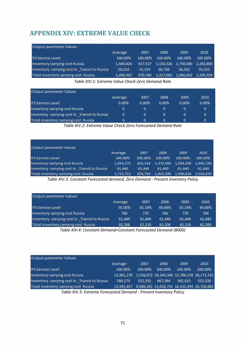
71

APPENDIX XIV: EXTREME VALUE CHECK

Table XIV.1: Extreme Value Check-Zero Demand Rate

Table XIV.2: Extreme Value Check-Zero Forecasted Demand Rate

Table XIV.3: Constant Forecasted demand, Zero Demand - Present Inventory Policy

Table XIV.4: Constant Demand=Constant Forecasted Demand (8000)

Table XIV.5: Extreme Forecasted Demand - Present Inventory Policy

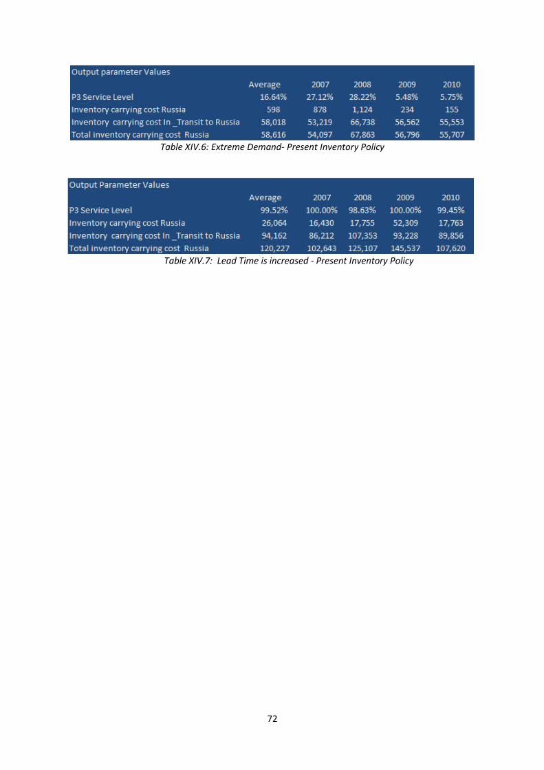
72

Table XIV.6: Extreme Demand- Present Inventory Policy

Table XIV.7: Lead Time is increased - Present Inventory Policy

73

APPENDIX XV: THE SIMULATION MODELS The inventory policies that were developed in chapters 4-5 were implemented in Excel worksheets

not only for comparing the results of the different policies but also in order to provide a tool for the

company. In this Appendix, the details of the simulation models that have been developed for each

alternative are presented. The same worksheet structure is used for the present inventory policies

and all the alternatives except for Alternative 4. The structure for Alternative 4 is slightly different

which was explained in XV.IV. Other than that some formulas are different depending on the

ordering rules of the inventory policies as explained in chapter 4-5.

The content of this Appendix is designed as follows: First of all, the screens of the simulation models

that the user can see the output parameter values and enter the input parameter values are

mentioned. Then, the structures of the simulation models are explained per each alternative. The

event occurrences for randomly selected 44 days (from day 731 to day 774) are illustrated for each

alternative. The algorithm of the simulation models (how values are calculated on each line) is

explained in detail through examples.

Appendix XV.I. The Structure of the Simulation Model -Present Inventory Policy

The Output/Input Screens of the Simulation Model: Table XV.I.1 illustrates the screen for analyzing the output results of the simulation models that have

been developed in chapter 7. Four output parameters are calculated: P3 service level, inventory

carrying cost at Stock Point 1 (Russia), inventory carrying cost in_transit from Stock Point 2 (USA) to

Stock Point 1 (Russia) and lastly total inventory carrying cost at Stock Point 1 (Russia). Service level is

calculated as a percentage and cost values are calculated in dollars.

Table XV.I.1 Output Screen of the Simulation Model – Present Inventory Policy

Table XV.I.2 shows the input parameter screen. The values that were entered are according to the

settings of the present inventory policy. It is possible for the user to play with the values. Review

period and lead time input parameters are mainly used for calculating the order shipment decisions

and output parameter service level. Product value ($) and carrying cost % are used for calculating

output cost parameters.

Table XV.I.2 Input Screen of the Simulation Model – Present Inventory Policy

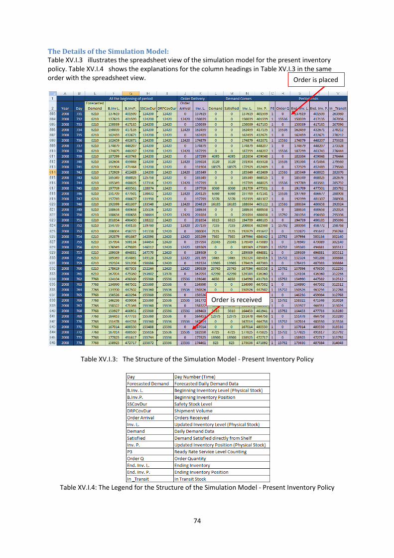
74

The Details of the Simulation Model: Table XV.I.3 illustrates the spreadsheet view of the simulation model for the present inventory policy. Table XV.I.4 shows the explanations for the column headings in Table XV.I.3 in the same order with the spreadsheet view.

Table XV.I.3: The Structure of the Simulation Model - Present Inventory Policy

Table XV.I.4: The Legend for the Structure of the Simulation Model - Present Inventory Policy

Order is received

Order is placed

75

The column notations of the spreadsheets (A, B, C etc. at the top of the sheets) are also used in

parenthesis for the explanation of the simulation logic below. Day 732 will be used as a starting

point for the explanation. In addition to input parameter values on the input screen (XV.II.2) , the

daily forecasted demand data (Column E) and daily actual demand data (Column L) are also input

parameters of the simulation model in the worksheets. The simulation model has four main parts as

follows: at the beginning of the period, order delivery, demand comes and finally period ends. The

details of each part were discussed below.

At the beginning of the period:

10. Simulation base time units are days. One year has 365 days. ‘Day’ Column (Column B)

indicates the day numbers.

20. ‘Forecasted Demand’ Column (Column E) includes the daily forecasted demand data.

30. On the first day of the simulation, initial values are assigned to ‘BInv L.’ and ‘BinvP.’ For the

rest of the days, at the beginning of each period, updated ‘BInv L.’ and ‘B.InvP.’ values are

calculated. ‘B.Inv.L.’ and ‘B.Inv.P’ levels equal ‘End. Inv.’ (Column S) and ‘End. Inv.P.’

(Column T) values of the previous day.

Example: Starting line Day 732

B.Inv. L.Day7322 (F804) = End.Inv. L.Day732 (S803)

B.Inv. P.Day732 (G804) = End.Inv. P.Day732(T803)

40. ‘SSCovDur’ (Column H) is used for calculating the safety stock level but this column is not

used in Present Inventory Policy (1).

Example: Starting line Day 732

= , where t is the day number

(E804: E823)

50. ‘DRPCovDur’ value on each line (Column H) equals to the sum of the 2 days of the forecasted

demand data. This column is used in the formula that decides on the shipment quantity

(Column R).

Example: Starting line Day 2

= , where t is the day number

(E804: E823)

Order Delivery :

60. ‘Order Arrival’ (Column J) includes the values for the daily received orders. Order that is

placed on day t (Column R) is received on day (t+ Lead Time) under this column.

Example: Starting line Day 732

70. ‘Inv. L’ Column (Column K) calculates the updated inventory level after receiving the order.

Example: Starting line Day 732

(K804) (F804) + ( J804)

76

Demand Comes :

80. ’Demand’ Column (Column L) includes the daily actual demand data.

90. ‘Satisfied’ Column (Column M) calculates how much demand data is satisfied directly from

the on hand inventory.

Example: Starting line Day 732

(L804),

100. ‘Inv. L.’ Column (Column N) calculates the inventory level after the daily demand is

subtracted. ‘Inv. L.’ Column value is decreased with the amount of the satisfied demand (Column

M).

Example: Starting line Day 732

(N804) = (K804) - (M804)

110. ‘Inv. P.’ Column (Column O) calculates the inventory position level after the demand

realization. ‘Inv. P’. Column value is decreased with the amount of satisfied demand

(Column M).

Example: Starting line Day 732

(M804)

Period Ends :

120. P3 Column (Column Q) is used for calculating the output parameter ‘P3 Service

Level’. P3 Column is calculated as follows:

If Inv. L. is greater than zero, it is 1. Otherwise it is 0.

Example: Starting line Day 732

Else P3Day 732 (Q804) =0

130. *Order Q (Column R) is used for order quantity decisions. If we are on the review

period day, then an order in the amount DRPCovDur value that is ‘Lead time’ (input

parameter value) days ahead is placed. This structure is illustrated with red arrows on Table

X.II.3

Example: Starting line Day 732

Then, it is review period day,

and order quantity is decided.

77

140. After the replenishment decision, End. Inv. L. (Column S) and End. Inv. P. (Column T)

levels are calculated. Ending inventory level is the same as the inventory level after the

satisfied demand. Inventory position is increased with the amount of ‘Order Q’.

Example: Starting line Day 732

150. In_Transit (Column V) is the difference between End.Inv.L. (Column S) and End.Inv.L.

(Column T).

Example: Starting line Day 732

Calculation of the Output Parameter Values :

10. P3 Service Level: In the company P3 service level is formulated as follows:

In the simulation output screen, P3 Service Level is calculated on the yearly level. Per each year,

P3 Column (Column Q) is summed and divided by the number of days in a year. Then, average

result is calculated based on the yearly results.

Example: Year 2008 - Starting line Day 731

(Rows : Q803-Q1167)

20. Inventory carrying cost Russia (Stock Point 1): Inventory carrying cost Russia is calculated

per each year separately using the input parameter values for ‘Product Value’, ‘Carrying Cost %’

and the daily ending inventory levels that are calculated under Column S . Then, overall average

result is calculated based on the yearly results.

Example: Year 2008 - Starting line Day 731

(Rows : Q803-Q1167)

30. Inventory carrying cost Russia (Stock Point 1): Inventory carrying cost In_Transit to Russia is

calculated per each year separately using the input parameter values ‘Product Value’, ‘Carrying Cost

78

%’ and the ending inventory levels that are calculated under Column S . Then, average result is

calculated based on the yearly results.

Example: Year 2008 - Starting line Day 731

(Rows: Q803-Q1167)

40. Total Inventory carrying cost Russia (Stock Point 1): Total inventory carrying cost Russia is

calculated as follows:

Appendix XV.II. The Structure of the Simulation Model –Alternative 1 Policy

The Output/Input Screens of the Simulation Model: Table XV.II.1 illustrates the screen for analyzing the output results of the simulation models that

have been developed in chapter 7. Four output parameters are calculated: P3 service level,

inventory carrying cost at Stock Point 1 (Russia), inventory carrying cost in_transit from Stock Point 2

(USA) to Stock Point 1 (Russia) and lastly total inventory carrying cost at Stock Point 1 (Russia).

Service level is calculated as a percentage and cost values are calculated in dollars.

Table XV.II.1 : Output Screen of the Simulation Model – Alternative 1

Table XV.II.2 shows the input parameter screen. The values that were entered are according to the

settings of Alternative 1. It is possible for the user to play with the values. Review period and lead

time input parameters are mainly used for calculating the order shipment decisions and output

parameter service level. Product value ($) and carrying cost % are used for calculating output cost

parameters.

Table XV.II.2 : Input Screen of the Simulation Model – Alternative 1

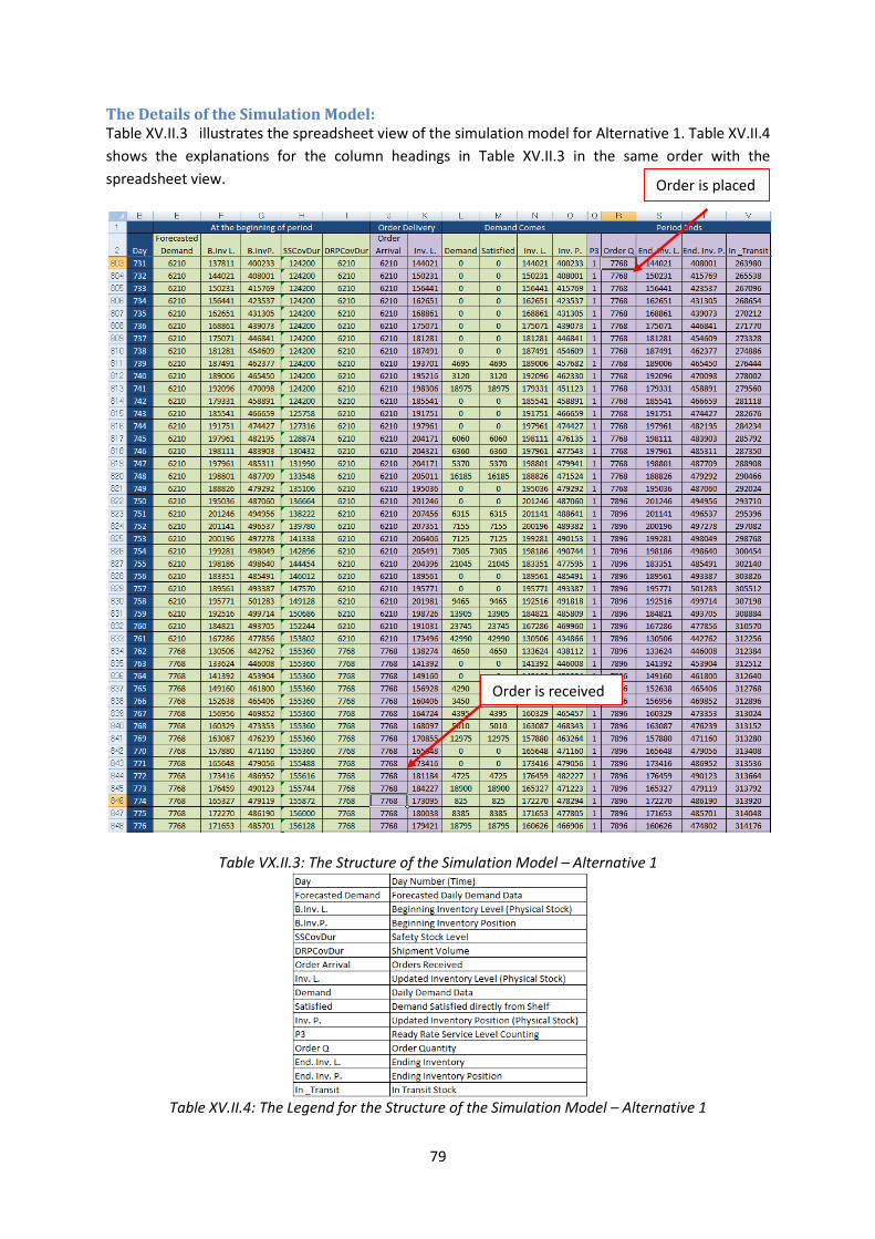
79

The Details of the Simulation Model: Table XV.II.3 illustrates the spreadsheet view of the simulation model for Alternative 1. Table XV.II.4

shows the explanations for the column headings in Table XV.II.3 in the same order with the

spreadsheet view.

Table VX.II.3: The Structure of the Simulation Model – Alternative 1

Table XV.II.4: The Legend for the Structure of the Simulation Model – Alternative 1

Order is received

Order is placed

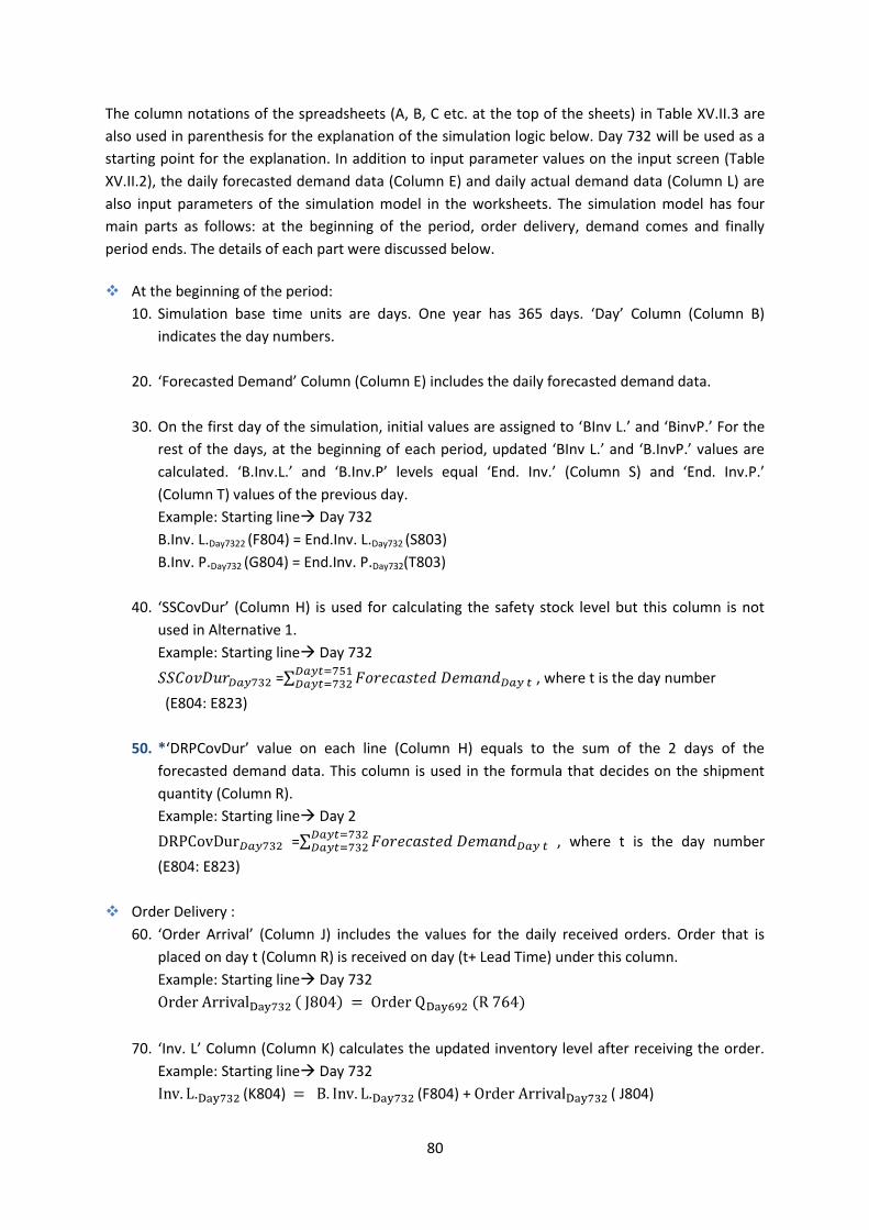
80

The column notations of the spreadsheets (A, B, C etc. at the top of the sheets) in Table XV.II.3 are

also used in parenthesis for the explanation of the simulation logic below. Day 732 will be used as a

starting point for the explanation. In addition to input parameter values on the input screen (Table

XV.II.2), the daily forecasted demand data (Column E) and daily actual demand data (Column L) are

also input parameters of the simulation model in the worksheets. The simulation model has four

main parts as follows: at the beginning of the period, order delivery, demand comes and finally

period ends. The details of each part were discussed below.

At the beginning of the period:

10. Simulation base time units are days. One year has 365 days. ‘Day’ Column (Column B)

indicates the day numbers.

20. ‘Forecasted Demand’ Column (Column E) includes the daily forecasted demand data.

30. On the first day of the simulation, initial values are assigned to ‘BInv L.’ and ‘BinvP.’ For the

rest of the days, at the beginning of each period, updated ‘BInv L.’ and ‘B.InvP.’ values are

calculated. ‘B.Inv.L.’ and ‘B.Inv.P’ levels equal ‘End. Inv.’ (Column S) and ‘End. Inv.P.’

(Column T) values of the previous day.

Example: Starting line Day 732

B.Inv. L.Day7322 (F804) = End.Inv. L.Day732 (S803)

B.Inv. P.Day732 (G804) = End.Inv. P.Day732(T803)

40. ‘SSCovDur’ (Column H) is used for calculating the safety stock level but this column is not

used in Alternative 1.

Example: Starting line Day 732

= , where t is the day number

(E804: E823)

50. *‘DRPCovDur’ value on each line (Column H) equals to the sum of the 2 days of the

forecasted demand data. This column is used in the formula that decides on the shipment

quantity (Column R).

Example: Starting line Day 2

= , where t is the day number

(E804: E823)

Order Delivery :

60. ‘Order Arrival’ (Column J) includes the values for the daily received orders. Order that is

placed on day t (Column R) is received on day (t+ Lead Time) under this column.

Example: Starting line Day 732

70. ‘Inv. L’ Column (Column K) calculates the updated inventory level after receiving the order.

Example: Starting line Day 732

(K804) (F804) + ( J804)

81

Demand Comes :

80. ’Demand’ Column (Column L) includes the daily actual demand data.

90. ‘Satisfied’ Column (Column M) calculates how much demand data is satisfied directly from

the on hand inventory.

Example: Starting line Day 732

(L804),

100. ‘Inv. L.’ Column (Column N) calculates the inventory level after the daily demand is

subtracted. ‘Inv. L.’ Column value is decreased with the amount of the satisfied demand (Column

M).

Example: Starting line Day 732

(N804) = (K804) - (M804)

110. ‘Inv. P.’ Column (Column O) calculates the inventory position level after the demand

realization. ‘Inv. P’. Column value is decreased with the amount of satisfied demand

(Column M).

Example: Starting line Day 732

(M804)

Period Ends :

120. P3 Column (Column Q) is used for calculating the output parameter ‘P3 Service

Level’. P3 Column is calculated as follows:

If Inv. L. is greater than zero, it is 1. Otherwise it is 0.

Example: Starting line Day 732

Else P3Day 732 (Q804) =0

130. *Order Q (Column R) is used for order quantity decisions. If we are on the review

period day, then an order in the amount DRPCovDur value that is ‘Lead time’ (input

parameter value) days ahead is placed. This structure is illustrated with red arrows on Table

X.III.3.

Example: Starting line Day 732

Then, it is review period day,

and order quantity is decided.

82

140. After the replenishment decision, End. Inv. L. (Column S) and End. Inv. P. (Column T)

levels are calculated. Ending inventory level is the same as the inventory level after the

satisfied demand. Inventory position is increased with the amount of ‘Order Q’.

Example: Starting line Day 732

150. In_Transit (Column V) is the difference between End.Inv.L. (Column S) and End.Inv.L.

(Column T).

Example: Starting line Day 732

Calculation of the Output Parameter Values :

10. P3 Service Level: In the company P3 service level is formulated as follows:

In the simulation output screen, P3 Service Level is calculated on the yearly level. Per each year,

P3 Column (Column Q) is summed and divided by the number of days in a year. Then, average

result is calculated based on the yearly results.

Example: Year 2008 - Starting line Day 731

(Rows : Q803-Q1167)

20. Inventory carrying cost Russia (Stock Point 1): Inventory carrying cost Russia is calculated

per each year separately using the input parameter values for ‘Product Value’, ‘Carrying Cost %’

and the daily ending inventory levels that are calculated under Column S . Then, overall average

result is calculated based on the yearly results.

Example: Year 2008 - Starting line Day 731

(Rows : Q803-Q1167)

30. Inventory carrying cost Russia (Stock Point 1): Inventory carrying cost In_Transit to Russia is

calculated per each year separately using the input parameter values ‘Product Value’, ‘Carrying Cost

83

%’ and the ending inventory levels that are calculated under Column S . Then, average result is

calculated based on the yearly results.

Example: Year 2008 - Starting line Day 731

(Rows: Q803-Q1167)

40. Total Inventory carrying cost Russia (Stock Point 1): Total inventory carrying cost Russia is

calculated as follows:

Appendix XV.III. The Structure of the Simulation Model –Alternative 2 Policy

The Output/Input Screens of the Simulation Model: Table XV.III.1 illustrates the screen for analyzing the output results of the simulation models that

have been developed in chapter 7. Four output parameters are calculated: P3 service level,

inventory carrying cost at Stock Point 1 (Russia), inventory carrying cost in_transit from Stock Point 2

(USA) to Stock Point 1 (Russia) and lastly total inventory carrying cost at Stock Point 1 (Russia).

Service level is calculated as a percentage and cost values are calculated in dollars.

Table XV.III.1 Output Screen of the Simulation Model – Alternative 2

Table XV.III.2 shows the input parameter screen. The values that were entered are according to the

settings of Alternative 2. It is possible for the user to play with the values. Review period and lead

time input parameters are mainly used for calculating the order shipment decisions and output

parameter service level. Product value ($) and carrying cost % are used for calculating output cost

parameters.

Table XV.III.2 Input Screen of the Simulation Model – Alternative 2

84

The Details of the Simulation Model: Table XV.III.3 illustrates the spreadsheet view of the simulation model for Alternative 2. Table

XV.III.4 shows the explanations for the column headings in Table XV.III.3 in the same order with the

spreadsheet view.

Table XV.III.3: The Structure of the Simulation Model – Alternative 2

Table XV.III.4: The Legend for the Structure of the Simulation Model – Alternative 2

Order is received

Order is placed

85

The column notations of the spreadsheets (A, B, C etc. at the top of the sheets) in Table XV.III.3 are

also used in parenthesis for the explanation of the simulation logic below. Day 732 will be used as a

starting point for the explanation. In addition to input parameter values on the input screen (Table

XV.III.2), the daily forecasted demand data (Column E) and daily actual demand data (Column L) are

also input parameters of the simulation model in the worksheets. The simulation model has four

main parts as follows: at the beginning of the period, order delivery, demand comes and finally

period ends. The details of each part were discussed below.

At the beginning of the period:

10. Simulation base time units are days. One year has 365 days. ‘Day’ Column (Column B)

indicates the day numbers.

20. ‘Forecasted Demand’ Column (Column E) includes the daily forecasted demand data.

30. On the first day of the simulation, initial values are assigned to ‘BInv L.’ and ‘BinvP.’ For the

rest of the days, at the beginning of each period, updated ‘BInv L.’ and ‘B.InvP.’ values are

calculated. ‘B.Inv.L.’ and ‘B.Inv.P’ levels equal ‘End. Inv.’ (Column S) and ‘End. Inv.P.’

(Column T) values of the previous day.

Example: Starting line Day 732

B.Inv. L.Day7322 (F804) = End.Inv. L.Day732 (S803)

B.Inv. P.Day732 (G804) = End.Inv. P.Day732(T803)

40. *‘SSCovDur’ (Column H) is used for calculating the safety stock level .

Example: Starting line Day 732

= , where t is the

day number

(E805: E844)

50. *‘DRPCovDur’ value on each line (Column H) equals to one day forecasted demand data. This

column is used in the formula that decides on the shipment quantity (Column R).

Example: Starting line Day 2

= , where t is the day number

(E804)

Order Delivery :

60. ‘Order Arrival’ (Column J) includes the values for the daily received orders. Order that is

placed on day t (Column R) is received on day (t+ Lead Time) under this column.

Example: Starting line Day 732

70. ‘Inv. L’ Column (Column K) calculates the updated inventory level after receiving the order.

Example: Starting line Day 732

(K804) (F804) + ( J804)

86

Demand Comes :

80. ’Demand’ Column (Column L) includes the daily actual demand data.

90. ‘Satisfied’ Column (Column M) calculates how much demand data is satisfied directly from

the on hand inventory.

Example: Starting line Day 732

(L804),

100. ‘Inv. L.’ Column (Column N) calculates the inventory level after the daily demand is

subtracted. ‘Inv. L.’ Column value is decreased with the amount of the satisfied demand (Column

M).

Example: Starting line Day 732

(N804) = (K804) - (M804)

110. ‘Inv. P.’ Column (Column O) calculates the inventory position level after the demand

realization. ‘Inv. P’. Column value is decreased with the amount of satisfied demand

(Column M).

Example: Starting line Day 732

(M804)

Period Ends :

120. P3 Column (Column Q) is used for calculating the output parameter ‘P3 Service

Level’. P3 Column is calculated as follows:

If Inv. L. is greater than zero, it is 1. Otherwise it is 0.

Example: Starting line Day 732

Else P3Day 732 (Q804) =0

130. *Order Q (Column R) is used for order quantity decisions. If we are on the review

period day, then an order in the amount DRPCovDur value that is ‘Lead time’ (input

parameter value) days ahead is placed. This structure is illustrated with red arrows on Table

X.IV.3.

Example: Starting line Day 732

Then, it is review period day,

and order quantity is decided.

87

(O804) > +

(Rows E805:E844), where t is the day number.

140. After the replenishment decision, End. Inv. L. (Column S) and End. Inv. P. (Column T)

levels are calculated. Ending inventory level is the same as the inventory level after the

satisfied demand. Inventory position is increased with the amount of ‘Order Q’.

Example: Starting line Day 732

150. In_Transit (Column V) is the difference between End.Inv.L. (Column S) and End.Inv.L.

(Column T).

Example: Starting line Day 732

Calculation of the Output Parameter Values :

10. P3 Service Level: In the company P3 service level is formulated as follows:

In the simulation output screen, P3 Service Level is calculated on the yearly level. Per each year,

P3 Column (Column Q) is summed and divided by the number of days in a year. Then, average

result is calculated based on the yearly results.

Example: Year 2008 - Starting line Day 731

(Rows : Q803-Q1167)

20. Inventory carrying cost Russia (Stock Point 1): Inventory carrying cost Russia is calculated

per each year separately using the input parameter values for ‘Product Value’, ‘Carrying Cost %’

and the daily ending inventory levels that are calculated under Column S . Then, overall average

result is calculated based on the yearly results.

Example: Year 2008 - Starting line Day 731

88

(Rows : Q803-Q1167)

30. Inventory carrying cost Russia (Stock Point 1): Inventory carrying cost In_Transit to Russia is

calculated per each year separately using the input parameter values ‘Product Value’, ‘Carrying Cost

%’ and the ending inventory levels that are calculated under Column S . Then, average result is

calculated based on the yearly results.

Example: Year 2008 - Starting line Day 731

(Rows: Q803-Q1167)

40. Total Inventory carrying cost Russia (Stock Point 1): Total inventory carrying cost Russia is

calculated as follows:

The Graphical Results of the Simulation Model Figure XV.III.1 and Figure XV.III.2 shows the time-based behavior of inventory position, safety stock

level, ordering rule threshold value and finally the ordering quantity.

Figure XV.III.1: Analysis for timely behavior of inventory position, safety stock level and threshold

value for the ordering rule.

Figure XV.III.2: Analysis for timely behavior of ordering quantity.

89

Appendix XV.IV. The Structure of the Simulation Model –Alternative 3 Policy

The Output/Input Screens of the Simulation Model: Table XV.IV.1 illustrates the screen for analyzing the output results of the simulation models that

have been developed in chapter 7. Four output parameters are calculated: P3 service level,

inventory carrying cost at Stock Point 1 (Russia), inventory carrying cost in_transit from Stock Point 2

(USA) to Stock Point 1 (Russia) and lastly total inventory carrying cost at Stock Point 1 (Russia).

Service level is calculated as a percentage and cost values are calculated in dollars.

Table XV.IV.1 Output Screen of the Simulation Model – Alternative 3

Table XV.IV.2 shows the input parameter screen. The values that were entered are according to the

settings of Alternative 3. It is possible for the user to play with the values. Review period and lead

time input parameters are mainly used for calculating the order shipment decisions and output

parameter service level. Product value ($) and carrying cost % are used for calculating output cost

parameters.

Table XV.IV.2 Input Screen of the Simulation Model – Alternative 3

90

The Details of the Simulation Model: Table XV.IV.3 illustrates the spreadsheet view of the simulation model for Alternative 3. Table

XV.IV.4 shows the explanations for the column headings in Table XV.IV.3 in the same order with the

spreadsheet view.

Table XV.IV.3: The Structure of the Simulation Model – Alternative 3

Table XV.IV.4: The Legend for the Structure of the Simulation Model – Alternative 3

Order is received

Order is placed

91

The column notations of the spreadsheets (A, B, C etc. at the top of the sheets) in Table XV.IV.3 are

also used in parenthesis for the explanation of the simulation logic below. Day 732 will be used as a

starting point for the explanation. In addition to input parameter values on the input screen (Table

XV.IV.2), the daily forecasted demand data (Column E) and daily actual demand data (Column L) are

also input parameters of the simulation model in the worksheets. The simulation model has four

main parts as follows: at the beginning of the period, order delivery, demand comes and finally

period ends. The details of each part were discussed below.

At the beginning of the period:

10. Simulation base time units are days. One year has 365 days. ‘Day’ Column (Column B)

indicates the day numbers.

20. ‘Forecasted Demand’ Column (Column E) includes the daily forecasted demand data.

30. On the first day of the simulation, initial values are assigned to ‘BInv L.’ and ‘BinvP.’ For the

rest of the days, at the beginning of each period, updated ‘BInv L.’ and ‘B.InvP.’ values are

calculated. ‘B.Inv.L.’ and ‘B.Inv.P’ levels equal ‘End. Inv.’ (Column S) and ‘End. Inv.P.’

(Column T) values of the previous day.

Example: Starting line Day 732

B.Inv. L.Day7322 (F804) = End.Inv. L.Day732 (S803)

B.Inv. P.Day732 (G804) = End.Inv. P.Day732(T803)

40. *‘SSCovDur’ (Column H) is used for calculating the safety stock level .

Example: Starting line Day 732

= , where t is the

day number

(E805: E844)

50. *‘DRPCovDur’ value on each line (Column H) equals to one day forecasted demand data. This

column is used in the formula that decides on the shipment quantity (Column R).

Example: Starting line Day 2

= , where t is the day number

(E804)

Order Delivery :

60. ‘Order Arrival’ (Column J) includes the values for the daily received orders. Order that is

placed on day t (Column R) is received on day (t+ Lead Time) under this column.

Example: Starting line Day 732

70. ‘Inv. L’ Column (Column K) calculates the updated inventory level after receiving the order.

Example: Starting line Day 732

(K804) (F804) + ( J804)

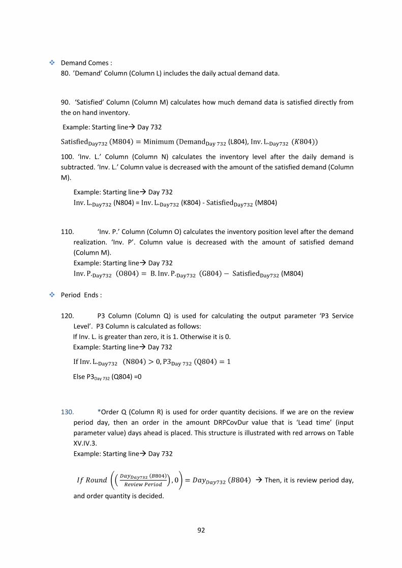
92

Demand Comes :

80. ’Demand’ Column (Column L) includes the daily actual demand data.

90. ‘Satisfied’ Column (Column M) calculates how much demand data is satisfied directly from

the on hand inventory.

Example: Starting line Day 732

(L804),

100. ‘Inv. L.’ Column (Column N) calculates the inventory level after the daily demand is

subtracted. ‘Inv. L.’ Column value is decreased with the amount of the satisfied demand (Column

M).

Example: Starting line Day 732

(N804) = (K804) - (M804)

110. ‘Inv. P.’ Column (Column O) calculates the inventory position level after the demand

realization. ‘Inv. P’. Column value is decreased with the amount of satisfied demand

(Column M).

Example: Starting line Day 732

(M804)

Period Ends :

120. P3 Column (Column Q) is used for calculating the output parameter ‘P3 Service

Level’. P3 Column is calculated as follows:

If Inv. L. is greater than zero, it is 1. Otherwise it is 0.

Example: Starting line Day 732

Else P3Day 732 (Q804) =0

130. *Order Q (Column R) is used for order quantity decisions. If we are on the review

period day, then an order in the amount DRPCovDur value that is ‘Lead time’ (input

parameter value) days ahead is placed. This structure is illustrated with red arrows on Table

XV.IV.3.

Example: Starting line Day 732

Then, it is review period day,

and order quantity is decided.

93

(O804) > +

(Rows E805:E844), where t is the day number.

140. After the replenishment decision, End. Inv. L. (Column S) and End. Inv. P. (Column T)

levels are calculated. Ending inventory level is the same as the inventory level after the

satisfied demand. Inventory position is increased with the amount of ‘Order Q’.

Example: Starting line Day 732

150. In_Transit (Column V) is the difference between End.Inv.L. (Column S) and End.Inv.L.

(Column T).

Example: Starting line Day 732

Calculation of the Output Parameter Values :

10. P3 Service Level: In the company P3 service level is formulated as follows:

In the simulation output screen, P3 Service Level is calculated on the yearly level. Per each year,

P3 Column (Column Q) is summed and divided by the number of days in a year. Then, average

result is calculated based on the yearly results.

Example: Year 2008 - Starting line Day 731

(Rows : Q803-Q1167)

20. Inventory carrying cost Russia (Stock Point 1): Inventory carrying cost Russia is calculated

per each year separately using the input parameter values for ‘Product Value’, ‘Carrying Cost %’

and the daily ending inventory levels that are calculated under Column S . Then, overall average

result is calculated based on the yearly results.

Example: Year 2008 - Starting line Day 731

94

(Rows : Q803-Q1167)

30. Inventory carrying cost Russia (Stock Point 1): Inventory carrying cost In_Transit to Russia is

calculated per each year separately using the input parameter values ‘Product Value’, ‘Carrying Cost

%’ and the ending inventory levels that are calculated under Column S . Then, average result is

calculated based on the yearly results.

Example: Year 2008 - Starting line Day 731

(Rows: Q803-Q1167)

40. Total Inventory carrying cost Russia (Stock Point 1): Total inventory carrying cost Russia is

calculated as follows:

The Graphical Results of the Simulation Model Figure XV.IV.1 and Figure XV.IV.2 shows the time-based behavior of inventory position, safety stock

level, ordering rule threshold value and finally the ordering quantity.

Figure XV.IV.1: Analysis for timely behavior of inventory position, safety stock level and threshold

value for the ordering rule.

Figure XV.IV.2: Analysis for timely behavior of ordering quantity.

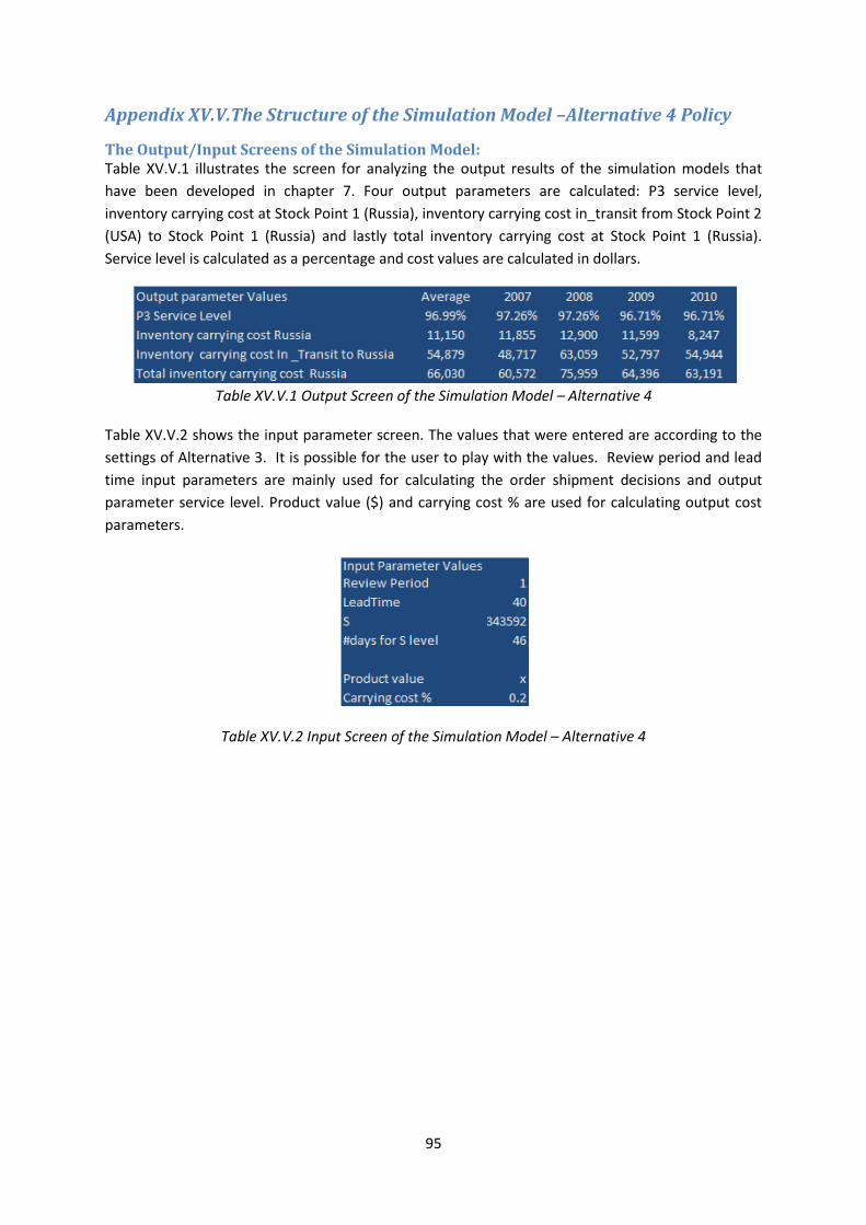
95

Appendix XV.V.The Structure of the Simulation Model –Alternative 4 Policy

The Output/Input Screens of the Simulation Model: Table XV.V.1 illustrates the screen for analyzing the output results of the simulation models that

have been developed in chapter 7. Four output parameters are calculated: P3 service level,

inventory carrying cost at Stock Point 1 (Russia), inventory carrying cost in_transit from Stock Point 2

(USA) to Stock Point 1 (Russia) and lastly total inventory carrying cost at Stock Point 1 (Russia).

Service level is calculated as a percentage and cost values are calculated in dollars.

Table XV.V.1 Output Screen of the Simulation Model – Alternative 4

Table XV.V.2 shows the input parameter screen. The values that were entered are according to the

settings of Alternative 3. It is possible for the user to play with the values. Review period and lead

time input parameters are mainly used for calculating the order shipment decisions and output

parameter service level. Product value ($) and carrying cost % are used for calculating output cost

parameters.

Table XV.V.2 Input Screen of the Simulation Model – Alternative 4

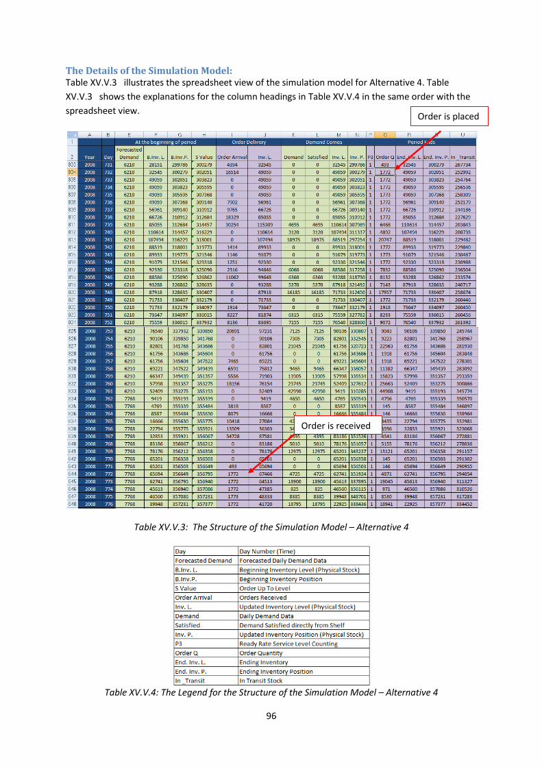
96

The Details of the Simulation Model: Table XV.V.3 illustrates the spreadsheet view of the simulation model for Alternative 4. Table

XV.V.3 shows the explanations for the column headings in Table XV.V.4 in the same order with the

spreadsheet view.

Table XV.V.3: The Structure of the Simulation Model – Alternative 4

Table XV.V.4: The Legend for the Structure of the Simulation Model – Alternative 4

Order is received

Order is placed

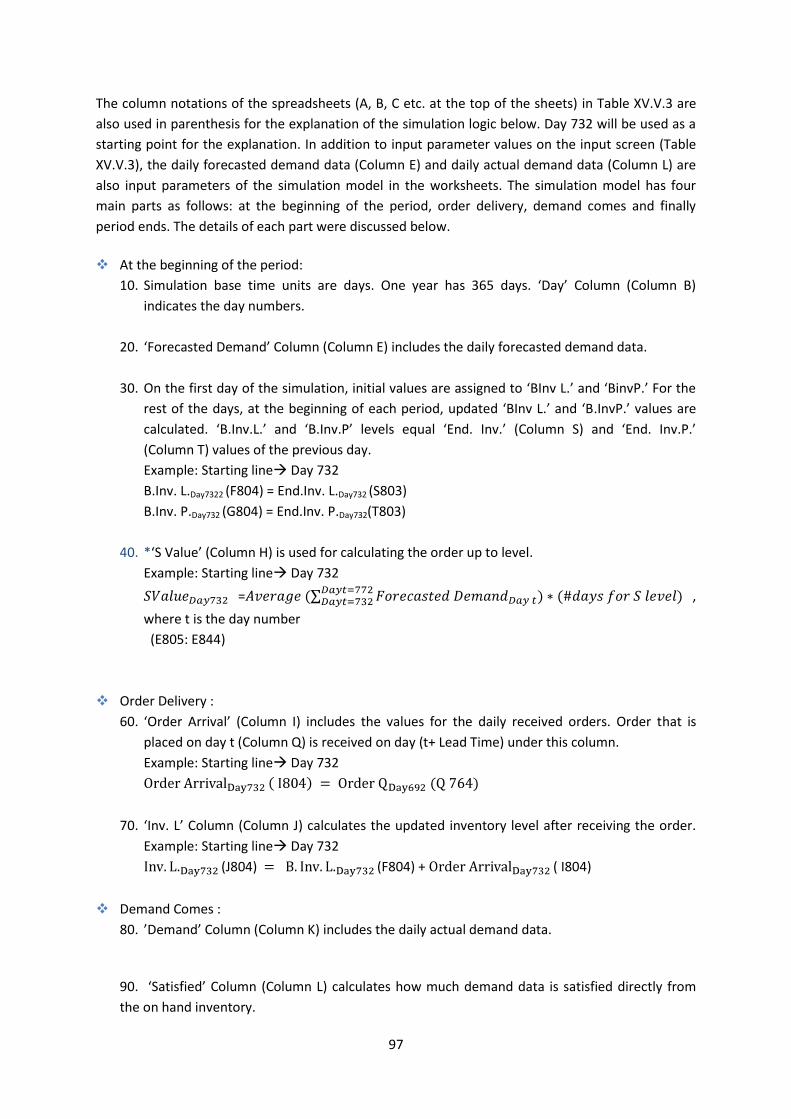
97

The column notations of the spreadsheets (A, B, C etc. at the top of the sheets) in Table XV.V.3 are

also used in parenthesis for the explanation of the simulation logic below. Day 732 will be used as a

starting point for the explanation. In addition to input parameter values on the input screen (Table

XV.V.3), the daily forecasted demand data (Column E) and daily actual demand data (Column L) are

also input parameters of the simulation model in the worksheets. The simulation model has four

main parts as follows: at the beginning of the period, order delivery, demand comes and finally

period ends. The details of each part were discussed below.

At the beginning of the period:

10. Simulation base time units are days. One year has 365 days. ‘Day’ Column (Column B)

indicates the day numbers.

20. ‘Forecasted Demand’ Column (Column E) includes the daily forecasted demand data.

30. On the first day of the simulation, initial values are assigned to ‘BInv L.’ and ‘BinvP.’ For the

rest of the days, at the beginning of each period, updated ‘BInv L.’ and ‘B.InvP.’ values are

calculated. ‘B.Inv.L.’ and ‘B.Inv.P’ levels equal ‘End. Inv.’ (Column S) and ‘End. Inv.P.’

(Column T) values of the previous day.

Example: Starting line Day 732

B.Inv. L.Day7322 (F804) = End.Inv. L.Day732 (S803)

B.Inv. P.Day732 (G804) = End.Inv. P.Day732(T803)

40. *‘S Value’ (Column H) is used for calculating the order up to level.

Example: Starting line Day 732

= ,

where t is the day number

(E805: E844)

Order Delivery :

60. ‘Order Arrival’ (Column I) includes the values for the daily received orders. Order that is

placed on day t (Column Q) is received on day (t+ Lead Time) under this column.

Example: Starting line Day 732

70. ‘Inv. L’ Column (Column J) calculates the updated inventory level after receiving the order.

Example: Starting line Day 732

(J804) (F804) + ( I804)

Demand Comes :

80. ’Demand’ Column (Column K) includes the daily actual demand data.

90. ‘Satisfied’ Column (Column L) calculates how much demand data is satisfied directly from

the on hand inventory.

98

Example: Starting line Day 732

(K804),

100. ‘Inv. L.’ Column (Column M) calculates the inventory level after the daily demand is

subtracted. ‘Inv. L.’ Column value is decreased with the amount of the satisfied demand (Column

L).

Example: Starting line Day 732

(M804) = (J804) - (L804)

110. ‘Inv. P.’ Column (Column N) calculates the inventory position level after the demand

realization. ‘Inv. P’. Column value is decreased with the amount of satisfied demand

(Column L).

Example: Starting line Day 732

(L804)

Period Ends :

120. P3 Column (Column P) is used for calculating the output parameter ‘P3 Service

Level’. P3 Column is calculated as follows:

If Inv. L. is greater than zero, it is 1. Otherwise it is 0.

Example: Starting line Day 732

Else P3Day 732 (P804) =0

130. *Order Q (Column Q) is used for order quantity decisions. If we are on the review

period day, then an order in the amount that increases the Inv. P. to SValue is placed. This

structure is illustrated with red arrows onTable X.VI.3

Example: Starting line Day 732

Then, it is review period day,

and order quantity is decided.

(N804) >

99

140. After the replenishment decision, End. Inv. L. (Column R) and End. Inv. P. (Column S)

levels are calculated. Ending inventory level is the same as the inventory level after the

satisfied demand. Inventory position is increased with the amount of ‘Order Q’.

Example: Starting line Day 732

150. In_Transit (Column U) is the difference between End.Inv.L. (Column R) and End.Inv.L.

(Column S).

Example: Starting line Day 732

Calculation of the Output Parameter Values :

10. P3 Service Level: In the company P3 service level is formulated as follows:

In the simulation output screen, P3 Service Level is calculated on the yearly level. Per each year,

P3 Column (Column Q) is summed and divided by the number of days in a year. Then, average

result is calculated based on the yearly results.

Example: Year 2008 - Starting line Day 731

(Rows : Q803-Q1167)

20. Inventory carrying cost Russia (Stock Point 1): Inventory carrying cost Russia is calculated

per each year separately using the input parameter values for ‘Product Value’, ‘Carrying Cost %’

and the daily ending inventory levels that are calculated under Column S . Then, overall average

result is calculated based on the yearly results.

Example: Year 2008 - Starting line Day 731

(Rows : Q803-Q1167)

30. Inventory carrying cost Russia (Stock Point 1): Inventory carrying cost In_Transit to Russia is

calculated per each year separately using the input parameter values ‘Product Value’, ‘Carrying Cost

%’ and the ending inventory levels that are calculated under Column S . Then, average result is

calculated based on the yearly results.

Example: Year 2008 - Starting line Day 731

100

(Rows: Q803-Q1167)

40. Total Inventory carrying cost Russia (Stock Point 1): Total inventory carrying cost Russia is

calculated as follows:

101

REFERENCES

Article and Book References

Bagchi, U., Hayya, J. C., Chu, C. H. (1986). The effect of lead-time variability: the case of independent

demand. The Journal of Operations Management, Vol.6, No.2, pp. 159-177.

Boulaksil Y., Fransoo, J.C., van Halm, E.N.G. (2007). Setting safety stocks in multi-stage inventory

systems under rolling horizon mathematical programming models. OR Spectrum, Vol. 31 No. 1, pp.

121-140.

Chang C.T., Lo T.Y (2009).On the inventory model with continuous and discrete lead time, backorders

and lost sales. Applied Mathematical Modeling, Vol.33, pp. 2196-2206.

Diks , E.B., de Kok, A.G., Lagodimos, A.G (1996). Multi-echelon systems: A service measure

perspective. European Journal of Operational Research, Vol. 95, No.2, pp. 241-263.

Kelton, W. D. , Sadowski, R.P. , Sturrock, D. T. (2003). Simulation with Arena, McGraw-Hill, New York;

Lau, H.S. , Zaki, A.,(1982). The sensitivity of inventory decisions to the shape of lead time demand distributions. IIE Transactions, Vol. 14, No. 4, pp. 265-271.

Law, A. M., Kelton, W. D. (1991). Simulation modeling and analysis. Third Edition. McGraw-Hill, New York.

Naddor,R. E. (1978). Sensitivity to distributions in inventory systems. Management Science, Vol. 24,

pp. 1769-1772.

Pibernik, R. (2006). Managing stock-outs effectively with order fulfillment systems. Journal of

Manufacturing Technology Management, Vol.17, No.6, pp. 721-736.

Silver, E.A. (1981). Operations Research in Inventory Management: A Review and Critique.

Operations Research, Vol. 29, No. 4, pp. 628-645.

Silver, E.A., Pyke, D.F., Peterson, R. (1998). Inventory management and production planning and

scheduling. Third Edition, John Wiley & Sons.

Schneider, H. (1981). Effect of service levels on order-points or order-levels in inventory models.

International Journal of Production Research, Vol.19, No.6, pp. 615-631.

Williams, B.D., Tokar, T. (2008). A review of inventory management research in major logistics

journals. Themes and future directions. The International Journal of Logistics Management, Vol. 19

No. 2, pp. 212-232.

102

Van Aken, J.E., Berends, J.J., & Van der Bij, J.D. (2007). Problem solving in organizations. Cambridge:

Cambridge University Press.

Van Strien, P.J. (1997). Towards a methodology of psychological practice. Theory and Psychology,Vol.

7 No.5, pp. 683-700.

Other Resources Uluc, T. (2010). MSc Preparation Report I-II. Hoover's Company Records. Austin: Aug 15, 2010. p. 40031 Hoover's Company Records. Austin: Aug 15, 2010. p. 100768 Hoover's Company Records. Austin: Aug 15, 2010. p. 110612 http://www.alticor.com http://www.quixtar.com http://www.amway.com http://www.accessbusinessgroup.com