1

Minimizing Earliness and Tardiness Costs in Stochastic Scheduling

By

Kenneth R. Baker

Tuck School of Business

Dartmouth College

Hanover, NH 03755

ken.baker@dartmouth.edu

(July, 2013)

Abstract

We address the single-machine stochastic scheduling problem with an objective of minimizing total

expected earliness and tardiness costs, assuming that processing times follow normal distributions and

due dates are decisions. We develop a branch and bound algorithm to find optimal solutions to this

problem and report the results of computational experiments. We also test some heuristic procedures

and find that surprisingly good performance can be achieved by a list schedule followed by an

adjacent pairwise interchange procedure.

2

Minimizing Earliness and Tardiness Costs in Stochastic Scheduling

1. Introduction

The single-machine sequencing model is the basic paradigm for scheduling theory. In its

deterministic version, the model has received a great deal of attention from researchers,

leading to problem formulations, solution methods, scheduling insights, and building blocks

for more complicated models. Extending that model into the realm of stochastic scheduling is

an attempt to make the theory more useful and practical. However, progress in analyzing

stochastic models has been much slower to develop, and even today some of the basic

problems remain virtually unsolved. One such case is the stochastic version of the

earliness/tardiness (E/T) problem for a single machine.

This paper presents a branch and bound (B&B) algorithm for solving the stochastic

E/T problem with normally-distributed processing times and due dates as decisions. This is

the first appearance of a solution algorithm more efficient than complete enumeration for this

problem, so we provide some experimental evidence on the algorithm’s computational

capability. In addition, we explore heuristic methods for solving the problem, and we show

that a relatively simple procedure can be remarkably successful at producing optimal or near-

optimal solutions. These results reinforce and clarify observations made in earlier research

efforts and ultimately provide us with a practical method of solving the stochastic E/T

problem with virtually any number of jobs.

In Section 2 we formulate the problem under consideration, and in Section 3 we

review the relevant literature. In Section 4, we describe the elements of the optimization

approach, and we report computational experience in Section 5. Section 6 deals with

heuristic procedures and the corresponding computational tests, and the final section provides

a summary and conclusions.

2. The Problem

In this paper we study the stochastic version of the single-machine E/T problem with due

dates as decisions. To start, we work with the basic single-machine sequencing model (Baker

and Trietsch, 2009a). In the deterministic version of this model, n jobs are available for

processing at time 0, and their parameters are known in advance. The key parameters in the

model include the processing time for job j (pj) and the due date (dj). In the actual schedule,

job j completes at time Cj, giving rise to either earliness or tardiness. The job’s earliness is

defined by Ej = max{0, dj − Cj} and its tardiness by Tj = max{0, Cj − dj}. Because the

economic implications of earliness and tardiness are not necessarily symmetric, the unit costs

3

of earliness (denoted by αj) and tardiness (denoted by βj) may be different. We express the

objective function, or total cost, as follows:

G(d1, d2, . . . , dn) = ∑ (1)

The deterministic version of this problem has been studied for over 30 years, and

several variations have been examined in the research literature. Some of these variations

have been solved efficiently, but most are NP-Hard problems. In the stochastic E/T problem,

we assume that the processing times are random variables, so the objective becomes the

minimization of the expected value of the function in (2). The stochastic version of the E/T

problem has not been solved.

To proceed with the analysis, we assume that the processing time pj follows a normal

distribution with mean j and standard deviation j and that the pj values are independent

random variables. We use the normal because it is familiar and plausible for many

scheduling applications. Few results in stochastic scheduling apply for arbitrary choices of

processing time distributions, so researchers have gravitated toward familiar cases that

resonate with the distributions deemed to be most practical. Several papers have addressed

stochastic scheduling problems and have used the normal distribution as an appropriate

model for processing times. Examples include Balut (1973), Sarin, et al. (1991), Fredendall

& Soroush (1994), Seo, et al. (1995), Cai & Zhou (1997), Soroush (1999), Jang (2002),

Portougal & Trietsch (2006), and Wu, et al. (2009).

In our model, the due dates dj are decisions and are not subject to randomness. The

objective function for the stochastic problem may be written as

H(d1, d2, . . . , dn) = E[G(d1, d2, . . . , dn)] =∑ (2)

The problem consists of finding a set of due dates and a sequence of the jobs that produce the

minimum value of the function in (2).

3. Literature Review

The model considered in this paper brings together several strands of scheduling research—

namely, earliness/tardiness criteria, due-date assignments, and stochastic processing times. We

trace the highlights of these themes in the subsections that follow.

3.1. Earliness/Tardiness Criteria

The advent of Just-In-Time scheduling spawned a segment of the literature that investigated cost

structures comprising both earliness costs and tardiness costs when processing times and due

4

dates are given. The concept was introduced by Sidney (1977), who analyzed the minimization

of maximum cost and by Kanet (1981), who analyzed the minimization of total absolute

deviation from a common due date, under the assumption that the due date is late enough that it

does not impose constraints on sequencing choices. This objective is equivalent to an E/T

problem in which the unit costs of earliness and tardiness are symmetric and the same for all

jobs. For this version of the problem, Hall, et al. (1991) developed an optimization algorithm

capable of solving problems with hundreds of jobs, even if the due date is restrictive. In addition,

Hall and Posner (1991) solved the version of the problem with symmetric earliness and tardiness

costs that vary among jobs. Their algorithm handles over a thousand jobs.

The case of distinct due dates is somewhat more challenging than the common due-date

model and not simply because more information is needed to specify the problem. For example,

in most variations of the common due-date problem, the optimal sequence is known to have a so-

called V shape, in which jobs in the first portion of the sequence appear in longest-first order,

followed by the remaining jobs in shortest-first order. (The number of V-shaped schedules is a

small subset of the number of possible sequences, especially as n grows large.) Another feature

of the common due-date problem is the possibility that the optimal solution may call for initial

idle time. However, inserted idle time is never advantageous once processing begins. In contrast,

when due dates are distinct, the role of inserted idle time is more complex: it may be optimal to

schedule inserted idle time at various places between the processing of jobs.

Garey, et al. (1988) showed that the E/T problem with distinct due dates is NP-Hard,

although, for a given sequence, the scheduling of idle time can be determined by an efficient

algorithm. Optimization approaches to the problem with distinct due dates were proposed and

tested by Abdul-Razaq & Potts (1988), Ow & Morton (1989), Yano & Kim (1991), Azizoglu, et

al. (1991), Kim & Yano (1994), Fry, et al. (1996), Li (1997), and Liaw (1999). Fry, et al.

addressed the special case in which earliness costs and tardiness costs are symmetric and

common to all jobs. Their B&B algorithm was able to solve problems with as many as 25 jobs.

Azizoglu, et al. addressed the version in which earliness costs and tardiness costs are common,

but not necessarily symmetric, and with inserted idle time prohibited. Their B&B algorithm

solved problems with up to 20 jobs. Abdul-Razaq & Potts developed a B&B algorithm for the

more general cost structure with distinct costs but with inserted idle time prohibited. Their

algorithm was able to solve problems up to about 25 jobs. (Their lower bound calculations,

however, use a dynamic program that is sensitive to the range of the processing times, which

they took to be [1, 10] in their test problems.) Li proposed an alternative lower bound calculation

for the same problem but still encountered computational difficulties in solving problems larger

than about 25 jobs. Liaw’s subsequent improvements extended this range to at least 30 jobs.

Because optimization methods have encountered lengthy computations times for

problems larger than about 25-30 jobs, much of the computational emphasis has been on

heuristic procedures. Ow & Morton were primarily interested in heuristic procedures for a

version of the problem that prohibits inserted idle time, but they utilized a B&B method to obtain

5

solutions (or at least good lower bounds) to serve as a basis for evaluating their heuristics. They

reported difficulty in finding optimal solutions to problems containing 15 jobs. Yano & Kim

compared several heuristics for the special case in which earliness and tardiness costs are

proportional to processing times. The B&B algorithm they used as a benchmark solved most of

their test problems up to about 16 jobs. Kim & Yano developed a B&B algorithm to solve the

special case in which earliness costs and tardiness costs are symmetric and identical. Their B&B

algorithm solved all of their test problems up to about 18 jobs. Lee & Choi (1995) reported

improved heuristic performance from a genetic algorithm. To compare heuristic methods, they

used lower bounds obtained from CPLEX runs that were often terminated after two hours of run

time, sometimes even for problems containing 15 jobs. James & Buchanan (1997) studied

variations on a tabu-search heuristic and used an integer program to produce optimal solutions

for problems up to 15 jobs.

Detailed reviews of this literature have been provided by Kanet & Sridharan (2000),

Hassin & Shani (2005) and M'Hallah (2007). The reason for mentioning problem sizes in these

studies, although they may be somewhat dated, is to contrast the limits on problem size

encountered in studies of the distinct due-date problem with those encountered in the common

due-date problem. This pattern suggests that stochastic versions of the problem may be quite

challenging when each job has its own due date.

3.2. Due-Date Assignments

The due-date assignment problem is familiar in the job shop context, in which due dates are

sometimes assigned internally as progress targets for scheduling. However, for our purposes, we

focus on single-machine cases. Perhaps the most extensively studied model involving due-date

assignment is the E/T problem with a common due date. The justification for this model is that it

applies to several jobs of a single customer, or alternatively, to several subassemblies of the same

final assembly. The E/T problem still involves choosing a due date and sequencing the jobs, but

the fact that only one due date exists makes the problem intrinsically different from the more

general case involving a distinct due date assignment for each job. Moreover, flexibility in due-

date assignment means that the choice of a due date can be made without imposing unnecessary

constraints on the problem, so formulations of the due date assignment problem usually

correspond to the common due-date problem with a given but nonrestrictive due date.

Panwalkar, et al. (1982) introduced the due-date assignment decision in conjunction with the

common due-date model, augmenting the objective function with a cost component for the lead

time. In their model, the unit earliness costs and unit tardiness costs are asymmetric but remain

the same across jobs. The results include a simple algorithm for finding the optimal due date.

Surveys of the common due-date assignment problem were later compiled by Baker & Scudder

6

(1990) and by Gordon, et al. (2002). As discussed below, however, very little of the work on

due-date assignment has dealt with stochastic models.

Actually, in the deterministic case, if due dates are distinct, then the due-date assignment

problem is trivial because earliness and tardiness can be avoided entirely. Baker & Bertrand

(1981), who examined heuristic rules for assigning due dates, such as those based on constant,

slack-based, or total-work leadtimes, also characterized the optimal due-date assignment when

the objective is to make the due dates as tight as possible. Seidmann, et al. (1981) proposed a

specialized variation of the single-machine model with unit earliness and tardiness costs common

to all jobs, augmenting the objective function with a cost component that penalizes loose due

dates if they exceed customers' reasonable and expected lead time. They provided an efficient

solution to that version of the problem as well. Other augmented models were addressed by

Shabtay (2008). Because the due-date assignment problem is easy to solve in the single-machine

case when due dates are distinct, papers on the deterministic model with distinct due dates

typically assume that due dates are given, and relatively few papers deal with distinct due dates

as decisions. When processing times are stochastic, however, the due-date assignment problem

becomes more difficult.

3.3. Stochastic Processing Times

The stochastic counterpart of a deterministic sequencing problem is defined by treating

processing times as uncertain and then minimizing the expected value of the original

performance measure. Occasionally, it is possible to substitute mean values for uncertain

processing times and simply call on results from deterministic analysis. This approach works for

the minimization of expected total weighted completion time, which is minimized by sequencing

the jobs in order of shortest weighted expected processing time, or SWEPT (Rothkopf, 1966).

Not only is SWEPT optimal, but the optimal value of expected total weighted completion time

can also be computed by replacing uncertain processing times by mean values and calculating

the total weighted completion time for the resulting deterministic model. For the minimization of

expected maximum tardiness, it is optimal to sequence the jobs in order of earliest due date, or

EDD (Crabill & Maxwell, 1969). However, replacing uncertain processing times by mean values

and calculating the deterministic objective function under EDD may not produce the correct

value for the stochastic objective function. In fact, suppressing uncertainty seldom leads to the

optimal solution of stochastic sequencing problems; problems that are readily solvable in the

deterministic case may be quite difficult to solve when it comes to their stochastic counterpart.

An example is the minimization of the number of stochastically tardy jobs (i.e., those that fail to

meet their prescribed service levels). Kise & Ibaraki (1973) showed that even this relatively

basic problem is NP-Hard.

7

Stochastic scheduling problems involving earliness and tardiness have rarely been

addressed in the literature. Cai & Zhou (1997) analyzed a stochastic version of the common due-

date problem with earliness and tardiness costs (augmented by a completion-time cost), with the

due date allowed to be probabilistic and the variance of each processing time distribution

assumed to be proportional to its mean. Although the proportionality condition makes the

problem a special case, it can at least be considered a stochastic counterpart of a deterministic

model discussed by Baker & Scudder (1990). Xia, et al. (2008) described a heuristic procedure to

solve the stochastic E/T problem with common earliness costs and common tardiness costs,

augmented by a cost component reflecting the tightness of the due dates. This formulation is the

stochastic counterpart of a special case of the problem analyzed by Seidmann, et al. (1981),

which was solved by an efficient algorithm.

The more general stochastic version of the common due-date problem has not been

solved, and only modest progress has been achieved on the stochastic E/T problem with distinct

due dates. Soroush & Fredendall (1994) analyzed a version of that problem with due dates given.

Soroush (1999) later proposed some heuristics for the version with due dates as decisions, and

Portougal & Trietsch (2006) showed that one of those heuristics was asymptotically optimal.

However, an optimization algorithm for that problem has not been developed and tested. Thus,

this paper develops an optimization algorithm to solve a problem that heretofore has been

attacked only with heuristic rules.

An alternative type of model for stochastic scheduling is based on machine breakdown

and repair as the source of uncertainty, as described by Birge, et al. (1990) and Al-Turki, et al.

(1997). In the breakdown-and-repair model, the source of uncertainty is the machine, whereas in

our model the source is the job, so the results tend not to overlap. Another alternative direction

for stochastic scheduling is represented in the techniques of robust scheduling. As originally

introduced by Daniels & Kouvelis (1995), robust scheduling aimed at finding the best worst-case

schedule for a given criterion. This approach, which is essentially equivalent to maximizing the

minimum payoff in decision theory, requires no distribution information and assumes only that

possible outcomes for each stochastic element can be identified but not their relative likelihoods.

On the other hand, β-robust scheduling, due to Daniels & Carrillo (1997), does use distribution

information in maximizing the probability that a given level of schedule performance will be

achieved. Nevertheless, the criterion to be optimized in this formulation is a probability rather

than an expected cost, and only an aggregate probability is pursued. For example, we might want

to maximize the probability that total completion time will be less than or equal to a given target

value. By contrast, the model we examine in this paper minimizes total expected cost as an

objective function, subject to a set of probabilities that apply individually to the jobs in the

schedule.

8

4. Analysis of the Stochastic Problem

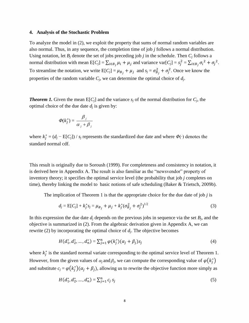
To analyze the model in (2), we exploit the property that sums of normal random variables are

also normal. Thus, in any sequence, the completion time of job j follows a normal distribution.

Using notation, let Bj denote the set of jobs preceding job j in the schedule. Then Cj follows a

normal distribution with mean E[Cj] = ∑ and variance var[Cj] =

= ∑

.

To streamline the notation, we write E[Cj] = and sj =

. Once we know the

properties of the random variable Cj, we can determine the optimal choice of dj.

Theorem 1. Given the mean E[Cj] and the variance sj of the normal distribution for Cj, the

optimal choice of the due date dj is given by:

Φ( ) =

jj

j

where = (dj − E[Cj]) / sj represents the standardized due date and where Φ(∙) denotes the

standard normal cdf.

This result is originally due to Soroush (1999). For completeness and consistency in notation, it

is derived here in Appendix A. The result is also familiar as the “newsvendor” property of

inventory theory; it specifies the optimal service level (the probability that job j completes on

time), thereby linking the model to basic notions of safe scheduling (Baker & Trietsch, 2009b).

The implication of Theorem 1 is that the appropriate choice for the due date of job j is

dj = E[Cj] + sj =

+ (

)

1/2 (3)

In this expression the due date dj depends on the previous jobs in sequence via the set Bj, and the

objective is summarized in (2). From the algebraic derivation given in Appendix A, we can

rewrite (2) by incorporating the optimal choice of dj. The objective becomes

= ∑

(4)

where is the standard normal variate corresponding to the optimal service level of Theorem 1.

However, from the given values of j and j, we can compute the corresponding value of ( )

and substitute cj = ( ) , allowing us to rewrite the objective function more simply as

= ∑

(5)

9

Having specified the objective function, we are interested in finding its optimal value. It

is possible, of course, to find an optimum by enumerating all possible job sequences and then

selecting the sequence with minimal objective function value. We refer to this procedure as

Algorithm E. Until now, enumeration has been the only solution algorithm for this problem, as in

Soroush (1999). However, enumerative methods are ultimately limited by the size of the solution

space. (Soroush reported obtaining solutions for 12-job problems in an average of over nine

hours of cpu time.) We can compute optimal solutions more efficiently with the use of a B&B

algorithm, which we describe next.

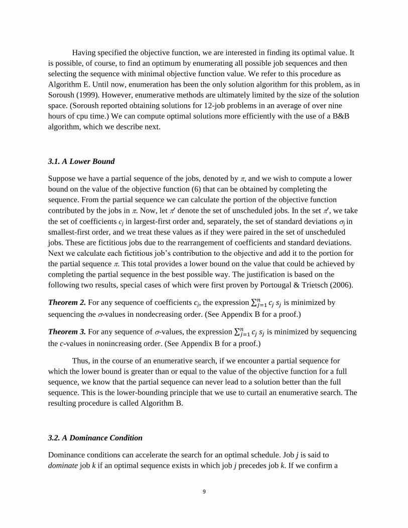
3.1. A Lower Bound

Suppose we have a partial sequence of the jobs, denoted by , and we wish to compute a lower

bound on the value of the objective function (6) that can be obtained by completing the

sequence. From the partial sequence we can calculate the portion of the objective function

contributed by the jobs in . Now, let ’ denote the set of unscheduled jobs. In the set ’, we take

the set of coefficients cj in largest-first order and, separately, the set of standard deviations j in

smallest-first order, and we treat these values as if they were paired in the set of unscheduled

jobs. These are fictitious jobs due to the rearrangement of coefficients and standard deviations.

Next we calculate each fictitious job’s contribution to the objective and add it to the portion for

the partial sequence . This total provides a lower bound on the value that could be achieved by

completing the partial sequence in the best possible way. The justification is based on the

following two results, special cases of which were first proven by Portougal & Trietsch (2006).

Theorem 2. For any sequence of coefficients cj, the expression ∑ is minimized by

sequencing the -values in nondecreasing order. (See Appendix B for a proof.)

Theorem 3. For any sequence of -values, the expression ∑ is minimized by sequencing

the c-values in nonincreasing order. (See Appendix B for a proof.)

Thus, in the course of an enumerative search, if we encounter a partial sequence for

which the lower bound is greater than or equal to the value of the objective function for a full

sequence, we know that the partial sequence can never lead to a solution better than the full

sequence. This is the lower-bounding principle that we use to curtail an enumerative search. The

resulting procedure is called Algorithm B.

3.2. A Dominance Condition

Dominance conditions can accelerate the search for an optimal schedule. Job j is said to

dominate job k if an optimal sequence exists in which job j precedes job k. If we confirm a

10

dominance condition of this type, then in searching for an optimal sequence we need not pursue

any partial sequence in which job k precedes job j. Dominance conditions can reduce the

computational effort required to find an optimal schedule, but the extent to which they apply

depends on the parameters in a given problem instance. For that reason, it may be difficult to

predict the extent of the improvement.

In our model, a relatively simple dominance condition holds.

Theorem 4. For two jobs j and k, if cj ≥ ck and j ≤ k then job j dominates job k.

Theorem 4, noted by Portougal & Trietsch (2006), can be proven by means of a pairwise

interchange argument, and the details appear in Appendix B for consistency in notation and level

of detail. Thus, if we are augmenting a partial sequence and we notice that job j dominates job k

while neither appears in the partial sequence, then we need not consider the augmented partial

sequence constructed by appending job k next. Although we may encounter quite a few

dominance properties in randomly-generated instances, it is also possible that no dominance

conditions hold. That would be the case if the costs and standard deviations were all ordered in

the same direction. In such a situation, dominance properties would not help reduce the

computational burden, and the computational effort involved in testing dominance conditions

would be counterproductive. We refer to the algorithm that checks dominance conditions as

Algorithm D.

Finally, we can implement lower bounds along with dominance conditions in the search.

We refer to this approach as Algorithm BD. Among the various algorithms, this combined

algorithm involves the most testing of conditions, but it can eliminate the most partial sequences.

In the next section we describe computational results for four versions: Algorithm E, Algorithm

B, Algorithm D, and Algorithm BD.

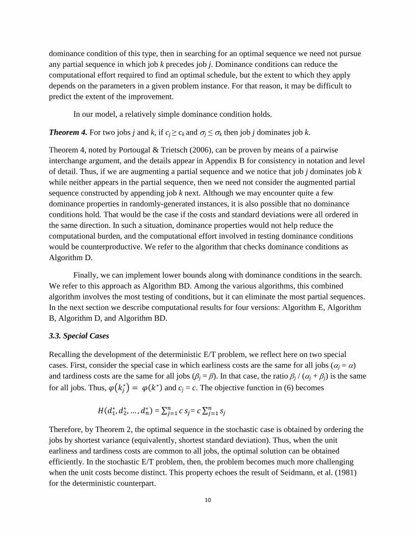
3.3. Special Cases

Recalling the development of the deterministic E/T problem, we reflect here on two special

cases. First, consider the special case in which earliness costs are the same for all jobs (j = )

and tardiness costs are the same for all jobs (j = ). In that case, the ratio j / (j + j) is the same

for all jobs. Thus, ( ) and cj = c. The objective function in (6) becomes

= ∑

= ∑

Therefore, by Theorem 2, the optimal sequence in the stochastic case is obtained by ordering the

jobs by shortest variance (equivalently, shortest standard deviation). Thus, when the unit

earliness and tardiness costs are common to all jobs, the optimal solution can be obtained

efficiently. In the stochastic E/T problem, then, the problem becomes much more challenging

when the unit costs become distinct. This property echoes the result of Seidmann, et al. (1981)

for the deterministic counterpart.

11

A further special case corresponds to the minimization of expected absolute deviation,

which corresponds to j = j = 1. In this case, the optimal sequence is again obtained by ordering

the jobs by shortest variance. In addition, = 0, so each job’s due date is optimally assigned to

the job’s expected completion time in the sequence. This property echoes the result of Baker &

Bertrand (1981) for the deterministic counterpart.

5. Computational Results for Optimization Methods

For experimental purposes, we generated a set of test problems that would permit comparisons of

the four algorithms. The mean processing times j were sampled from a uniform distribution

between 10 and 100. Then, for each job j, the standard deviation was sampled from a uniform

distribution between 0.10j and 0.25j. In other words, the mean was between 4 and 10 times the

standard deviation, so the chances of encountering a negative value for a processing time would

be negligible. (In other experimental work with the normal distribution, Xia, et al. (2008) also

generated mean values as small as 4 times the standard deviation; Soroush (1999) and Cai &

Zhou (2007) allowed for means as small as 3.4 times the standard deviation.) In addition, the unit

costs j and j were sampled independently from a uniform distribution between 1 and 10 on a

grid of 0.1. For each value of n (n = 6, 8, and 10), a sample of 100 randomly-generated problem

instances were created.

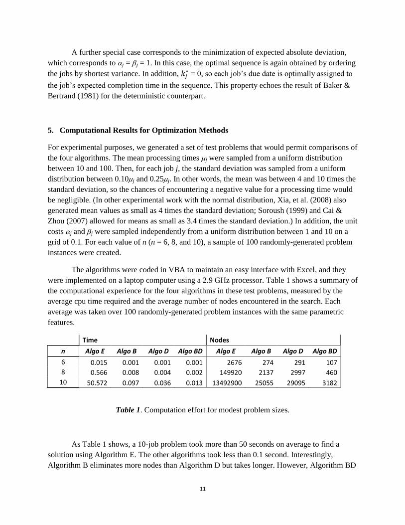
The algorithms were coded in VBA to maintain an easy interface with Excel, and they

were implemented on a laptop computer using a 2.9 GHz processor. Table 1 shows a summary of

the computational experience for the four algorithms in these test problems, measured by the

average cpu time required and the average number of nodes encountered in the search. Each

average was taken over 100 randomly-generated problem instances with the same parametric

features.

Time

Nodes

n Algo E Algo B Algo D Algo BD Algo E Algo B Algo D Algo BD

6 0.015 0.001 0.001 0.001 2676 274 291 107

8 0.566 0.008 0.004 0.002 149920 2137 2997 460

10 50.572 0.097 0.036 0.013 13492900 25055 29095 3182

Table 1. Computation effort for modest problem sizes.

As Table 1 shows, a 10-job problem took more than 50 seconds on average to find a

solution using Algorithm E. The other algorithms took less than 0.1 second. Interestingly,

Algorithm B eliminates more nodes than Algorithm D but takes longer. However, Algorithm BD

12

includes both types of conditions and is clearly the fastest. Thus, the use of dominance

conditions along with lower bounds provides the best performance. For Algorithm E,

computation times become prohibitive for larger problem sizes. In particular, 12-job problems

took roughly 1.7 hours with complete enumeration. (Compare the nine-hour solution times

reported by Soroush; the improvement here probably reflects advances in hardware since the

time of his experiments.)

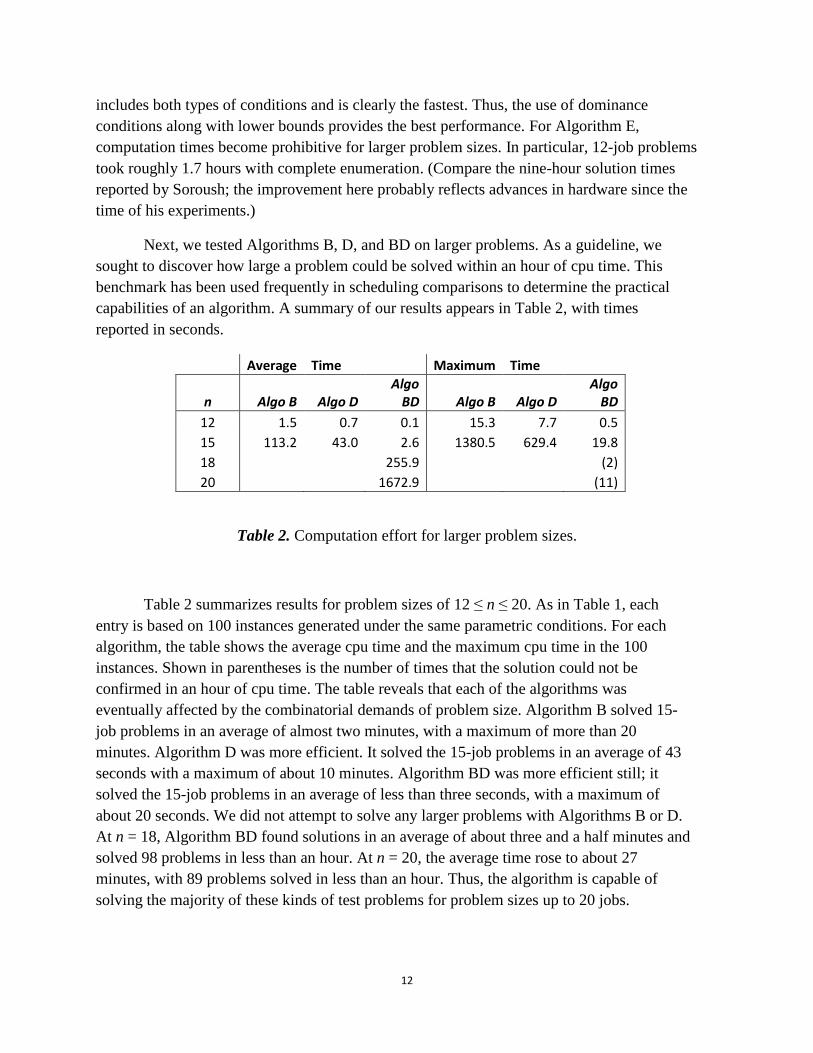
Next, we tested Algorithms B, D, and BD on larger problems. As a guideline, we

sought to discover how large a problem could be solved within an hour of cpu time. This

benchmark has been used frequently in scheduling comparisons to determine the practical

capabilities of an algorithm. A summary of our results appears in Table 2, with times

reported in seconds.

Average Time Maximum Time

n Algo B Algo D Algo

BD Algo B Algo D Algo

BD

12 1.5 0.7 0.1 15.3 7.7 0.5

15 113.2 43.0 2.6 1380.5 629.4 19.8

18

255.9

(2)

20 1672.9 (11)

Table 2. Computation effort for larger problem sizes.

Table 2 summarizes results for problem sizes of 12 ≤ n ≤ 20. As in Table 1, each

entry is based on 100 instances generated under the same parametric conditions. For each

algorithm, the table shows the average cpu time and the maximum cpu time in the 100

instances. Shown in parentheses is the number of times that the solution could not be

confirmed in an hour of cpu time. The table reveals that each of the algorithms was

eventually affected by the combinatorial demands of problem size. Algorithm B solved 15-

job problems in an average of almost two minutes, with a maximum of more than 20

minutes. Algorithm D was more efficient. It solved the 15-job problems in an average of 43

seconds with a maximum of about 10 minutes. Algorithm BD was more efficient still; it

solved the 15-job problems in an average of less than three seconds, with a maximum of

about 20 seconds. We did not attempt to solve any larger problems with Algorithms B or D.

At n = 18, Algorithm BD found solutions in an average of about three and a half minutes and

solved 98 problems in less than an hour. At n = 20, the average time rose to about 27

minutes, with 89 problems solved in less than an hour. Thus, the algorithm is capable of

solving the majority of these kinds of test problems for problem sizes up to 20 jobs.

13

6. Computational Results for Heuristic Methods

Because the stochastic E/T problem is difficult to solve optimally, it is relevant to explore

heuristic procedures that do not require extensive computing effort. In this section, we study

the performance of some heuristic procedures.

A simple and straightforward heuristic procedure is to create a list schedule. In other

words, the list of jobs is sorted in some way and then the schedule is implemented by

processing the jobs in their sorted order. In some stochastic scheduling models, sorting by

expected processing time can be effective, but in this problem, the optimal choice of the due

dates adjusts for differences in the jobs’ processing times. Instead, it makes sense to focus on

the standard deviations or variances of the processing times as a means of distinguishing the

jobs. The simplest way to do so is to sort the jobs by smallest standard deviation or by

smallest variance. Because the jobs are also distinguished by unit costs, it makes sense to

investigate cost-weighted versions of those orderings, such as smallest weighted standard

deviation (SWSD) and smallest weighted variance (SWV). Soroush (1999) tested list

schedules for these two rules and found that, at least on smaller problem sizes, they often

produced solutions within 1% of optimality.

A standard improvement procedure for sequencing problems is a neighborhood

search. In this case, we use a sorting rule to find an initial job sequence and then test adjacent

pairwise interchanges (API) in the schedule to seek an improvement. If an improvement is

found, the API neighborhood of the improved sequence is tested, and the process iterates

until no further improvement is possible. API methods have proven effective in solving

deterministic versions of the E/T problem, a finding that dates back to Yano & Kim (1991).

In our tests, API methods were remarkably effective.

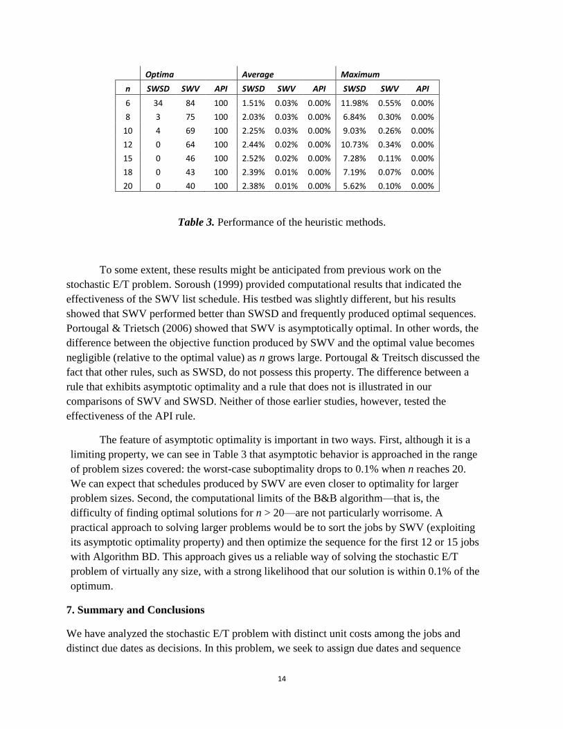
The quality of the heuristic solutions is summarized in Table 3 for the same set of test

problems described earlier. Three summary measures are of interest: (1) the number of

optima produced, (2) the average (relative) suboptimality, and (3) the maximum

suboptimality. As the table shows, the performances of the heuristic procedures were quite

different. The SWSD list schedule produced solutions that averaged about 2% above

optimal, and the SWV list schedule produced solutions that were two orders of magnitude

better. The SWV procedure also produced optimal solutions in about 60% of the test

problems. However, perhaps the most surprising result was that the API heuristic generated

optimal solutions in every one of the 700 test problems. (The API heuristic cannot guarantee

optimality, however. This point is discussed in Appendix C.)

14

Optima

Average

Maximum

n SWSD SWV API SWSD SWV API SWSD SWV API

6 34 84 100 1.51% 0.03% 0.00% 11.98% 0.55% 0.00%

8 3 75 100 2.03% 0.03% 0.00% 6.84% 0.30% 0.00%

10 4 69 100 2.25% 0.03% 0.00% 9.03% 0.26% 0.00%

12 0 64 100 2.44% 0.02% 0.00% 10.73% 0.34% 0.00%

15 0 46 100 2.52% 0.02% 0.00% 7.28% 0.11% 0.00%

18 0 43 100 2.39% 0.01% 0.00% 7.19% 0.07% 0.00%

20 0 40 100 2.38% 0.01% 0.00% 5.62% 0.10% 0.00%

Table 3. Performance of the heuristic methods.

To some extent, these results might be anticipated from previous work on the

stochastic E/T problem. Soroush (1999) provided computational results that indicated the

effectiveness of the SWV list schedule. His testbed was slightly different, but his results

showed that SWV performed better than SWSD and frequently produced optimal sequences.

Portougal & Trietsch (2006) showed that SWV is asymptotically optimal. In other words, the

difference between the objective function produced by SWV and the optimal value becomes

negligible (relative to the optimal value) as n grows large. Portougal & Treitsch discussed the

fact that other rules, such as SWSD, do not possess this property. The difference between a

rule that exhibits asymptotic optimality and a rule that does not is illustrated in our

comparisons of SWV and SWSD. Neither of those earlier studies, however, tested the

effectiveness of the API rule.

The feature of asymptotic optimality is important in two ways. First, although it is a

limiting property, we can see in Table 3 that asymptotic behavior is approached in the range

of problem sizes covered: the worst-case suboptimality drops to 0.1% when n reaches 20.

We can expect that schedules produced by SWV are even closer to optimality for larger

problem sizes. Second, the computational limits of the B&B algorithm—that is, the

difficulty of finding optimal solutions for n > 20—are not particularly worrisome. A

practical approach to solving larger problems would be to sort the jobs by SWV (exploiting

its asymptotic optimality property) and then optimize the sequence for the first 12 or 15 jobs

with Algorithm BD. This approach gives us a reliable way of solving the stochastic E/T

problem of virtually any size, with a strong likelihood that our solution is within 0.1% of the

optimum.

7. Summary and Conclusions

We have analyzed the stochastic E/T problem with distinct unit costs among the jobs and

distinct due dates as decisions. In this problem, we seek to assign due dates and sequence

15

the jobs so that the expected cost due to earliness and tardiness is as small as possible.

We first noted that the optimal assignment of due dates translates into a critical fractile

rule specifying the optimal service level for each job. We then described a B&B approach

to this problem, incorporating lower bounds and dominance conditions to reduce the

search effort. Our computational experiments indicated that the resulting algorithm

(Algorithm BD) can solve problems of up to around 20 jobs within an hour of cpu time.

Although these problem sizes might not seem large, computational experience for the

deterministic counterpart was seldom much better. In addition, the 20-job problem is

about twice the size of a problem that could be solved by enumeration in an hour of cpu

time.

We pointed out that a special case of this problem—when all jobs have identical

(but asymmetric) unit costs of earliness and tardiness—can be solved quite efficiently, by

sorting the jobs from smallest to largest variance. A cost-weighted version of this

procedure is not optimal in the general problem but appears to produce near-optimal

solutions reliably when used as a heuristic rule (Table 3). Moreover, when that solution is

followed with an Adjacent Pairwise Interchange neighborhood search for improvements,

the resulting algorithm produced optimal solutions in all of our test problems.

Our analysis was based on the assumption that processing times followed normal

distributions. The normal distribution is convenient because it implies that completion times

follow normal distributions as well. As Portugal & Trietsch (2006) observed, the role of

completion times in the objective function leads to the use of convolutions in the analysis.

Among standard probability distributions that could be used for processing times, only the

normal gives us the opportunity to rely on closed-form results. In place of the normal

distribution, we could assume that processing times follow lognormal distributions. The

lognormal is sometimes offered as a more practical representation of uncertain processing

times; indeed, it may be the most useful standard distribution for that purpose. However,

sums of lognormal distributions are not lognormal, implying that it would be difficult to

model completion times. Nevertheless, the lognormal is associated with a specialized central

limit theorem which resembles the familiar one that applies to the normal distribution

(Mazmanian, et al., 2008). In other words, our analysis for the normal could be adapted, at

least approximately, for the lognormal as well. However, by focusing here on the normal

distribution, our analysis has been exact, and no approximations have been necessary.

Looking back to the research done on the deterministic counterpart, we note that the

E/T model was sometimes augmented with an objective function component designed to

capture the tightness of due dates or to motivate short turnaround times. Augmenting the

stochastic E/T problem in such ways would appear to be a fruitful area in which to build on

this research.

16

References

Abdul-Razaq, T. and C. Potts (1988) Dynamic programming state-space relaxation for single-

machine scheduling. Journal of the Operational Research Society 39, 141-152.

Al-Turki, U., J. Mittenthal and M. Raghavachari (1996) The single-machine absolute-deviation

early-tardy problem with random completion times. Naval Research Logistics 43, 573-587.

Azizoglu M., S. Kondakci and O. Kirca (1991) Bicriteria scheduling problem involving total

tardiness and total earliness penalties. International Journal of Production Economics 23,

17–24.

Baker, K. and W. Bertrand (1981) A comparison of due-date selection rules. AIIE Transactions

13, 123–131.

Baker, K. and G. Scudder (1990) Sequencing with earliness and tardiness penalties: a

review. Operations Research 38, 22-36.

Baker, K. and D. Trietsch (2009a) Principles of Sequencing and Scheduling, John Wiley

& Sons, New York.

Baker, K. and D. Trietsch (2009b) Safe scheduling: setting due dates in single-machine

problems. European Journal of Operational Research 196, 69-77.

Balut, S., (1973) Scheduling to minimize the number of late jobs when set-up and processing

times are uncertain. Management Science 19, 1283–1288.

Birge, J., J. Frenk, J. Mittenthal, and A. Rinnooy Kan (1990) Single-machine scheduling subject

to stochastic breakdowns. Naval Research Logistics 31, 661-677.

Cai, X. and S. Zhou (2007) Scheduling stochastic jobs with asymmetric earliness and tardiness

penalties. Naval Research Logistics 44, 531–557.

Crabill, T. and W. Maxwell (1969) Single machine sequencing with random processing times

and random due-dates. Naval Research Logistics Quarterly 16, 549-555.

Daniels, R. and P. Kouvelis (1995) Robust scheduling to hedge against processing time

uncertainty in single-stage production. Management Science 41, 363-376.

Daniels, R. and J. Carrillo (1997) β-Robust scheduling for single-machine systems with

uncertain processing times. IIE Transactions 29, 977-985.

Fry, T., R. Armstrong and J. Blackstone (1987) Minimizing weighted absolute deviation in

single machine scheduling. IIE Transactions 19, 445–450.

17

Fry, T., R. Armstrong, K. Darby-Dowman and P. Philipoom (1996) A branch and bound

procedure to minimize mean absolute lateness on a single processor. Computers &

Operations Research 23, 171–182.

Garey, M., R. Tarjan and G. Wilfong (1988) One-Processor Scheduling with Symmetric

Earliness and Tardiness Penalties. Mathematics of Operations Research 13, 330-348.

Gordon, V., J-M. Proth and C. Chu (2002) A survey of the state-of-the-art of common due date

assignment and scheduling research. European Journal of Operational Research 139, 1–25.

Hall, N. and M. Posner (1991) Earliness-tardiness scheduling problems. I: Weighted deviation of

completion times about a common due date. Operations Research 39, 836–846.

Hall, N., W. Kubiak and S. Sethi (1991) Earliness-tardiness scheduling problems. II: Deviation

of completion times about a restrictive common due date. Operations Research, 39, 847–856.

Hassin, R. and M. Shani (2005) Machine scheduling with earliness, tardiness and non-execution

penalties. Computers & Operations Research 32, 683-705.

James, R. and J. Buchanan (1997) A neighbourhood scheme with a compressed solution space

for the early/tardy scheduling problem. European Journal of Operational Research 102, 513-

527.

Jang, W. (2002) Dynamic scheduling of stochastic jobs on a single machine, European Journal

of Operational Research 138, 518–530.

Kanet, J. (1981) Minimizing the average deviation of job completion times about a common due

date. Naval Research Logistics Quarterly 28, 643-651.

Kanet, J. and V. Sridharan (2000) Scheduling with Inserted Idle Time: Problem Taxonomy and

Literature Review. Operations Research 48, 99-110.

Kim, H. and C. Yano (1994) Minimizing mean tardiness and earliness in single-machine

scheduling problems with unequal due dates. Naval Research Logistics 41, 913-933.

Kise, H. and T. Ibaraki (1983) On Balut’s algorithm and NP-completeness for a chance-

constrained scheduling problem. Management Science 29, 384–388.

Lee, C. and J. Choi (1995) A genetic algorithm for job sequencing problems with distinct due

dates and general early-tardy penalty weights. Computers & Operations Research 22, 857–

869.

Li, G. (1997) Single machine earliness and tardiness scheduling. European Journal of

Operational Research 96, 546–558.

Liaw, C. (1999) A branch and bound algorithm for the single machine earliness and tardiness

scheduling problem. Computers & Operations Research 26, 679–693.

18

Mazmanian, L., V. Ohanian and D. Trietsch (2008) The lognormal central limit theorem

for positive random variables. Working Paper. Reproduced within the Research Notes

for Appendix A at http://mba.tuck.dartmouth.edu/pss/.

M'Hallah, R. (2007) Minimizing total earliness and tardiness on a single machine using a hybrid

heuristic. Computers & Operations Research 34, 3126 – 3142.

Ow, P. and T. Morton (1989) The single machine early/tardy problem. Management Science 35,

177-191.

Panwalkar, S., M. Smith and A. Seidmann (1982) Common due date assignment to minimize

total penalty for the one machine scheduling problem. Operations Research 30, 391–399.

Rothkopf, M. (1966) Scheduling with random service times. Management Science 12, 707-713.

Portougal, V. and D. Trietsch (2006) Setting due dates in a stochastic single machine

environment. Computers & Operations Research 33, 1681-1694.

Sarin, S., E. Erdel and G. Steiner (1991) Sequencing jobs on a single machine with a common

due date and stochastic processing times. European Journal of Operational Research 27,

188–198.

Seidmann, A., S. Panwalkar and M. Smith (1981) Optimal assignment of due-dates for a single

processor scheduling problem. International Journal of Production Research 19,393–399.

Seo, D., C. Klein and W. Jang (2005) Single machine stochastic scheduling to minimize the

expected number of tardy jobs using mathematical programming models. Computers &

Industrial Engineering 48, 153-161.

Shabtay D. (2008) Due date assignments and scheduling a single machine with a general

earliness/tardiness cost function. Computers & Operations Research 35, 1539–1545.

Sidney, J. (1977) Optimal single-machine scheduling with earliness and tardiness penalties.

Operations Research 25, 62-69.

Soroush, H. and L. Fredendall (1994) The stochastic single machine scheduling problem with

earliness and tardiness costs. European Journal of Operational Research 77, 287–302.

Soroush, H. (1999) “Sequencing and due-date determination in the stochastic single machine

problem with earliness and tardiness costs,” European Journal of Operations Research 113,

450–468.

Wu, C., K. Brown and J. Beck (2009) Scheduling with uncertain durations: Modeling β-robust

scheduling with constraints. Computers & Operations Research 36, 2348–2356.

19

Xia, Y., B. Chen and J. Yue (2008) Job sequencing and due date assignment in a single machine

shop with uncertain processing times. European Journal of Operational Research 184, 63-

75.

Yano, C., and Y. Kim, (1991) Algorithms for a class of single-machine tardiness and earliness

problems, European Journal of Operational Research, 52, 167–178.

20

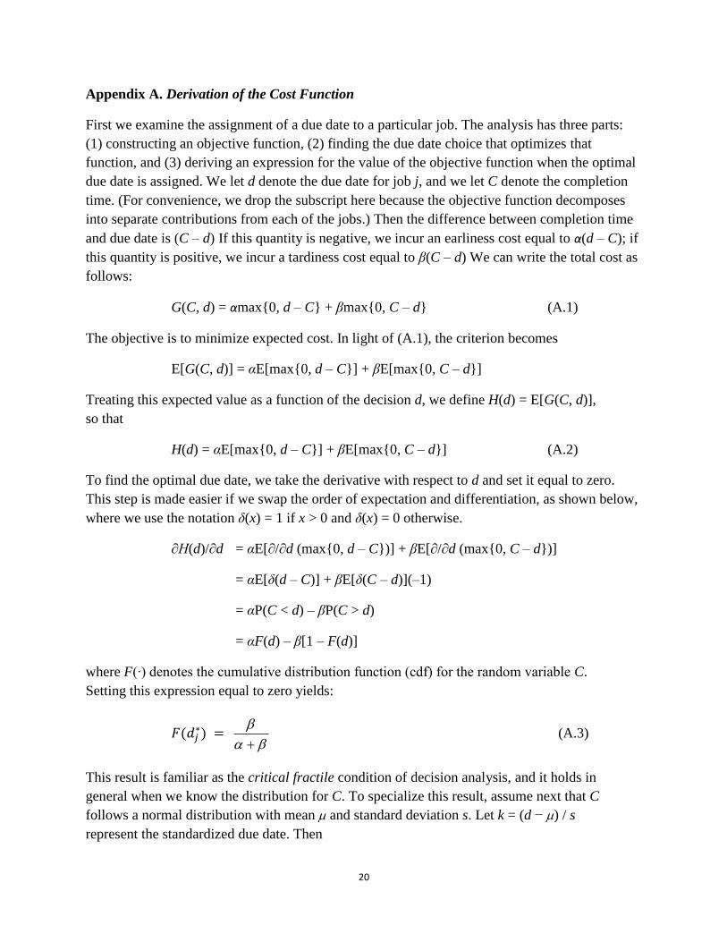
Appendix A. Derivation of the Cost Function

First we examine the assignment of a due date to a particular job. The analysis has three parts:

(1) constructing an objective function, (2) finding the due date choice that optimizes that

function, and (3) deriving an expression for the value of the objective function when the optimal

due date is assigned. We let d denote the due date for job j, and we let C denote the completion

time. (For convenience, we drop the subscript here because the objective function decomposes

into separate contributions from each of the jobs.) Then the difference between completion time

and due date is (C – d) If this quantity is negative, we incur an earliness cost equal to α(d – C); if

this quantity is positive, we incur a tardiness cost equal to β(C – d) We can write the total cost as

follows:

G(C, d) = αmax{0, d – C} + βmax{0, C – d} (A.1)

The objective is to minimize expected cost. In light of (A.1), the criterion becomes

E[G(C, d)] = αE[max{0, d – C}] + βE[max{0, C – d}]

Treating this expected value as a function of the decision d, we define H(d) = E[G(C, d)],

so that

H(d) = αE[max{0, d – C}] + βE[max{0, C – d}] (A.2)

To find the optimal due date, we take the derivative with respect to d and set it equal to zero.

This step is made easier if we swap the order of expectation and differentiation, as shown below,

where we use the notation δ(x) = 1 if x > 0 and δ(x) = 0 otherwise.

∂H(d)/∂d = αE[∂/∂d (max{0, d – C})] + βE[∂/∂d (max{0, C – d})]

= αE[δ(d – C)] + βE[δ(C – d)](–1)

= αP(C < d) – βP(C > d)

= αF(d) – β[1 – F(d)]

where F(∙) denotes the cumulative distribution function (cdf) for the random variable C.

Setting this expression equal to zero yields:

(A.3)

This result is familiar as the critical fractile condition of decision analysis, and it holds in

general when we know the distribution for C. To specialize this result, assume next that C

follows a normal distribution with mean and standard deviation s. Let k = (d − ) / s

represent the standardized due date. Then

21

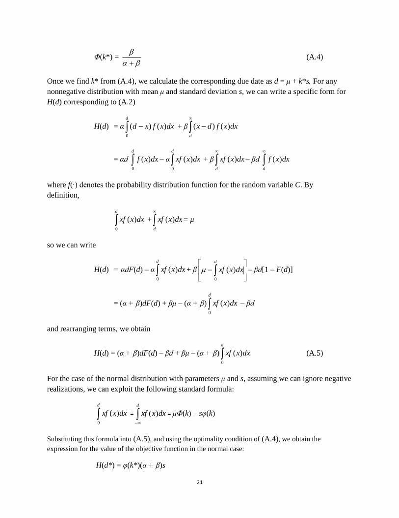
Φ(k*) =

(A.4)

Once we find k* from (A.4), we calculate the corresponding due date as d = μ + k*s For any

nonnegative distribution with mean μ and standard deviation s, we can write a specific form for

H(d) corresponding to (A.2)

H(d) = α

d

dxxfxd0

)()( + β

d

dxxfdx )()(

= αd d

dxxf0

)( – α d

dxxxf0

)( + β

d

dxxxf )( – βd

d

dxxf )(

where f(∙) denotes the probability distribution function for the random variable C. By

definition,

d

dxxxf0

)( +

d

dxxxf )( = µ

so we can write

H(d) = αdF(d) – α d

dxxxf0

)( + β

d

dxxxf0

)( – βd[1 – F(d)]

= (α + β)dF(d) + βμ – (α + β) d

dxxxf0

)( – βd

and rearranging terms, we obtain

H(d) = (α + β)dF(d) – βd + βμ – (α + β) d

dxxxf0

)( (A.5)

For the case of the normal distribution with parameters μ and s, assuming we can ignore negative

realizations, we can exploit the following standard formula:

d

dxxxf0

)( =

d

dxxxf )( = μΦ(k) – sφ(k)

Substituting this formula into (A.5), and using the optimality condition of (A.4), we obtain the

expression for the value of the objective function in the normal case:

H(d*) = φ(k*)(α + β)s

22

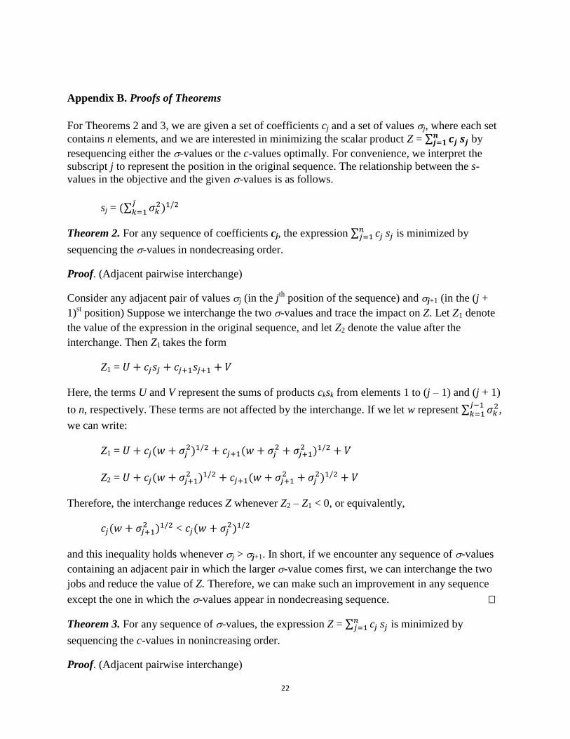
Appendix B. Proofs of Theorems

For Theorems 2 and 3, we are given a set of coefficients cj and a set of values j, where each set

contains n elements, and we are interested in minimizing the scalar product Z = ∑ by

resequencing either the -values or the c-values optimally. For convenience, we interpret the

subscript j to represent the position in the original sequence. The relationship between the s-

values in the objective and the given -values is as follows.

sj = ∑

Theorem 2. For any sequence of coefficients cj, the expression ∑ is minimized by

sequencing the -values in nondecreasing order.

Proof. (Adjacent pairwise interchange)

Consider any adjacent pair of values j (in the jth

position of the sequence) and j+1 (in the (j +

1)st position) Suppose we interchange the two -values and trace the impact on Z. Let Z1 denote

the value of the expression in the original sequence, and let Z2 denote the value after the

interchange. Then Z1 takes the form

Z1 =

Here, the terms U and V represent the sums of products cksk from elements 1 to (j – 1) and (j + 1)

to n, respectively. These terms are not affected by the interchange. If we let w represent ∑

,

we can write:

Z1 =

Z2 =

Therefore, the interchange reduces Z whenever Z2 – Z1 < 0, or equivalently,

<

and this inequality holds whenever j > j+1. In short, if we encounter any sequence of -values

containing an adjacent pair in which the larger -value comes first, we can interchange the two

jobs and reduce the value of Z. Therefore, we can make such an improvement in any sequence

except the one in which the -values appear in nondecreasing sequence.

Theorem 3. For any sequence of -values, the expression Z = ∑ is minimized by

sequencing the c-values in nonincreasing order.

Proof. (Adjacent pairwise interchange)

23

Consider any adjacent pair of values cj (in the jth

position of the sequence) and cj+1 (in the (j + 1)st

position) Suppose we interchange the two cj-values and trace the impact on Z. Let Z1 denote the

value of the expression in the original sequence, and let Z2 denote the value after the interchange.

Then Z1 takes the form

Z1 =

Here, the terms U and V represent the sums of products cksk from elements 1 to (j – 1) and (j + 1)

to n, respectively. These terms are not affected by the interchange. Thus, we can write:

Z1 =

Z2 =

Therefore, the interchange reduces Z whenever Z2 – Z1 < 0, or equivalently,

<

<

<

Because the variance is positive, this inequality holds whenever cj < cj+1. In short, if we encounter

any sequence of c-values containing an adjacent pair in which the smaller c-value comes first, we

can make a pairwise interchange and reduce the value of Z. Therefore, we can make such an

improvement in any sequence except the one in which the c-values appear in nonincreasing

sequence.

Lemma 1. Given two pairs of positive constants aj ≥ ak and bj < bk then

ajbj + akbk ≤ ajbk + akbj

In other words, the scalar product of the a’s and b’s is minimized by pairing larger a with smaller

b and smaller a with larger b.

Proof.

Because bk – bj > 0, we can write aj(bk – bj) ≥ ak(bk – bj) The inequality in the Lemma follows

algebraically.

Theorem 4. For two jobs j and k, if cj ≥ ck and j ≤ k then job j dominates job k.

Proof. (Pairwise interchange)

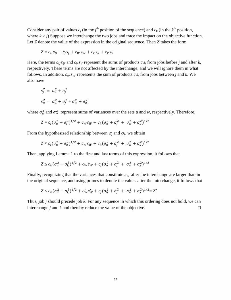
24

Consider any pair of values cj (in the jth

position of the sequence) and ck (in the kth

position,

where k > j) Suppose we interchange the two jobs and trace the impact on the objective function.

Let Z denote the value of the expression in the original sequence. Then Z takes the form

Z =

Here, the terms and represent the sums of products cisi from jobs before j and after k,

respectively. These terms are not affected by the interchange, and we will ignore them in what

follows. In addition, represents the sum of products cisi from jobs between j and k. We

also have

+

where and

represent sums of variances over the sets u and w, respectively. Therefore,

Z =

From the hypothesized relationship between j and k, we obtain

Z ≤

Then, applying Lemma 1 to the first and last terms of this expression, it follows that

Z ≤

Finally, recognizing that the variances that constitute after the interchange are larger than in

the original sequence, and using primes to denote the values after the interchange, it follows that

Z <

=

Thus, job j should precede job k. For any sequence in which this ordering does not hold, we can

interchange j and k and thereby reduce the value of the objective.

25

Appendix C. Examples of Suboptimality for the API Rule

The neighborhood search heuristic, based on adjacent pairwise interchange (API) neighborhoods,

provides surprising performance at finding optimal solutions in the basic test instances.

However, for the API Rule to be optimal, it would have to produce no local optima except at the

optimum. In that case, it would be possible to construct the optimal sequence by starting with

any sequence and implementing a sequence of adjacent interchanges, each one improving the

objective function, until the optimum is reached. The following three-job example contains a

local optimum and thus demonstrates that adjacent pairwise interchanges may not always deliver

the optimal solution.

job 1 2 3

10 10 10

1.70 1.87 1.40

1.07 2.00 0.64

1.70 1.40 1.20

Table C1. A three-job example.

Suppose we begin with the sequence 1-2-3. Calculations for the data in Table C1 will confirm

that the objective function is 7.110 for this solution. Two neighboring sequences are accessible

via adjacent interchanges. Their objective function values are 7.122 (for 1-3-2) and 7.117 (for 2-

1-3) Therefore, if we begin the search with the sequence 1-2-3, we find it to be a local optimum,

and we would not search beyond its neighborhood. However, the optimal solution is actually 3-

2-1, with a value of 7.105.

Although the three-job example illustrates that the API rule is not transitive, it happens

that the application of the API Rule to a starting sequence produced by SWV will yield an

optimal solution. In Table C2, we provide a six-job instance in which SWV followed by API

does not produce an optimal solution.

job 1 2 3 4 5 6

20 30 40 50 60 70

1.00 1.40 2.25 3.00 3.50 4.00

0.5 1.2 4 8 12 18

9.5 10 15 22 28 32

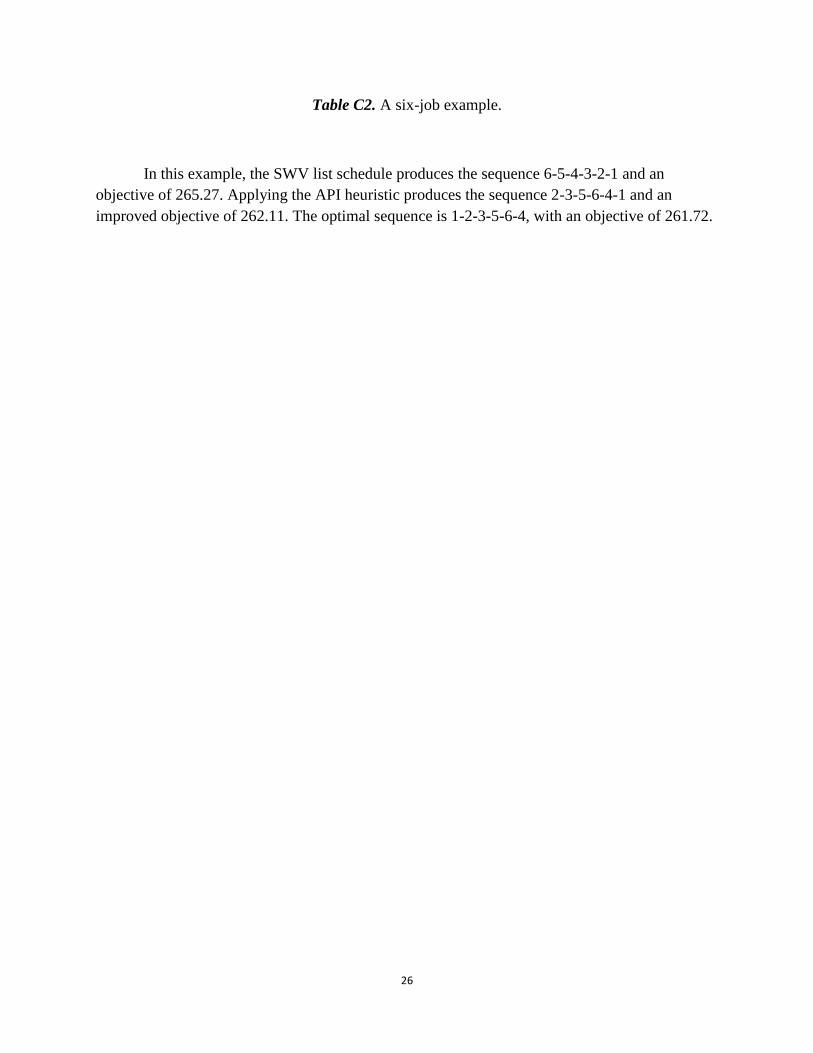
26

Table C2. A six-job example.

In this example, the SWV list schedule produces the sequence 6-5-4-3-2-1 and an

objective of 265.27. Applying the API heuristic produces the sequence 2-3-5-6-4-1 and an

improved objective of 262.11. The optimal sequence is 1-2-3-5-6-4, with an objective of 261.72.