Minimize Labeling Effort for Tree SkeletonSegmentation using an Automated Iterative Training

Methodology

Keenan Granland, Rhys Newbury, Zijue Chen, David Ting, Chao Chen∗

Laboratory of Motion Generation and Analysis, Faculty of Engineering, Monash University,Clayton, VIC 3800, Australia

Abstract

Training of convolutional neural networks for semantic segmentation requires

accurate pixel-wise labeling which requires large amounts of human effort. The

human-in-the-loop method reduces labeling effort; however, it requires human

intervention for each image. This paper describes a general iterative training

methodology for semantic segmentation, Automating-the-Loop. This aims to

replicate the manual adjustments of the human-in-the-loop method with an au-

tomated process, hence, drastically reducing labeling effort. Using the applica-

tion of detecting partially occluded apple tree segmentation, we compare manu-

ally labeled annotations, self-training, human-in-the-loop, and Automating-the-

Loop methods in both the quality of the trained convolutional neural networks,

and the effort needed to create them. The convolutional neural network (U-Net)

performance is analyzed using traditional metrics and a new metric, Complete

Grid Scan, which promotes connectivity and low noise. It is shown that in our

application, the new Automating-the-Loop method greatly reduces the labeling

effort while producing comparable performance to both human-in-the-loop and

complete manual labeling methods.

Keywords: Self-Training, Semantic Segmentation, Semi-supervised Learning,

Computer Vision, Agricultural Engineering

∗Corresponding authorEmail address: chao.chen@monash.edu (Chao Chen)

Preprint submitted to Computers and Electronics in Agriculture August 10, 2021

arX

iv:2

010.

0829

6v3

[cs

.CV

] 9

Aug

202

1

1. Introduction

Automation in agriculture is becoming increasingly viable as technology ad-

vances become more accessible. However, this technology is faced with many

challenges due to the environmental variations on farms. Current robotic solu-

tions require highly structured environments with flat ground, wide rows, and5

two-dimensional trellised tree structures. In reality, each farm has a unique

method of shaping trees using different patterns depending on the apple vari-

ety, land, environment, and the farmers’ preference.

One of the significant challenges in fruit harvesting is modeling the complex

environment. Accurately detecting tree skeletons can lead to increased total10

harvest and minimize damage to trees. Tree skeletons are typically occluded

by leaves, fruits, and other farming structures. To mitigate occlusions, tree

skeletons can be detected during dormant seasons (Majeed et al., 2020).

In the process of detecting branches and trunks of trees, labeling is commonly

done through object detection (box labels) (Kang and Chen, 2020). However,15

for some applications, such as harvesting, thinning, and pruning of fruit trees,

accurate modeling of the branches is required to proceed. As such, pixel-based

labeling is required, which requires a large amount of human effort (Chen et al.,

2021), as shown in Figure 1.

To train deep learning models for semantic segmentation, accurate pixel20

by pixel labeling of possibly hundreds of thousands of images is needed for

training (Ulku and Akagunduz, 2020). To reduce this effort, researchers have

explored Human-Machine Collaboration to reduce the human effort required in

labeling data. For example, human-in-the-loop (HITL) assisted labeling, where

a human annotator corrects the output of a neural network, reducing the to-25

tal labeling effort. Castrejon et al. (2017) developed Polygon-RNN, which uses

a polygon annotation tool to allow the human to quickly modify segmenta-

tion outputs speeding up the annotation by a factor 4.7 across all classes in

Cityscapes (Cordts et al., 2016).

2

Figure 1: Examples of RGB image of a tree (top row) and the corresponding manually labeled

data (bottom row).

Recently, active learning has been used to automatically select a subset of30

data to be manually annotated. Ravanbakhsh et al. (2019) use the discriminator

of a generative adversarial network (GAN) to identify unreliable labels for which

the export annotation is required. If the discriminator is confident, they use

the generator to directly synthesize samples. Zhang and Chen (2002) and Tong

and Chang (2001) utilize attribute probabilities and effective relevance feedback35

algorithms to extract the most informative images for manual annotation from

a large static pool. While these methods reduce the labeling effort required,

they still require human assistance throughout the whole process.

In domains where additional labeling of images is not a viable option, other

forms of semi-supervised learning have been proposed without the need for ad-40

ditional labeling. Semi-supervised learning is a general field in machine learning

that trains supervised models using unlabeled data (Zhu and Goldberg, 2009).

The goal of semi-supervised learning is to achieve better results than what can

be achieved with supervised learning when there is access to a larger amount of

3

unlabeled data. To achieve this, many semi-supervised methodologies rely on a45

strong high-quality supervised baseline to build upon (Zhu and Goldberg, 2009).

The simplest form of semi-supervised learning is to utilize predictions from an

unlabeled data-set in training directly (Lee et al., 2017). However, this has is-

sues with self-biasing as well as perpetuating mistakes. Many semi-supervised

learning models attempt to resolve the perpetuating error problem by adding50

confident predictions (psuedo-labels) in to an updated training set. This is often

called self-training (Lee et al., 2017). For example, classifier models can output

a confidence rating which can be used to select predictions for training based

on a confidence threshold (Zhu and Goldberg, 2009) or custom scoring metrics

external to the model can be used (Ouali et al., 2020b). Other methods have55

utilized these scores not to threshold but instead to weight the training labels

created from the model (Ouali et al., 2020a).

Yao et al. (2020) proposed a dynamic curriculum learning strategy, which

makes used of a self-training method to learn from feeding training images of in-

creasing difficulty, which requires accurate difficulty evaluation. These methods60

have shown that the creation of accurate and specific scoring algorithms can be

a powerful tool in enabling the use of unlabeled data for training. Sun et al.

(2020) proposed the Boundary-Aware Semi-Supervised Semantic Segmentation

Network for high resolution remote sensing, that improves results without ad-

ditional annotation workload by using custom processes to alleviate boundary65

blur.

In this paper, we introduce a general iterative training method for Convolu-

tional Neural Networks (CNNs) to increase the accuracy of the network. This

work aims to train a CNN to accurately detect and label tree skeletons from a

small set of data, minimizing the total human effort required. We trained a se-70

mantic segmentation CNN (U-Net) in an iterative process to provide pixel-wise

labels for Y-shaped apple tree skeletons. This was achieved using an automated

method aiming to replicate the human adjustments from the human-in-the-

loop process. The performance of each stage in the iterative training process

is analyzed. Four different methods are outlined, explored, and compared to75

4

determine the effectiveness of each. Mean IOU and Boundary F1 are used to

evaluate performance. Also, a custom scoring metric, Complete Grid Scan, is

introduced to give a better comparison of the performance in this application.

The contributions of this paper are:

1. Introduction of the Iterative Training Methodology for semi-supervised80

semantic segmentation learning.

2. Introduction of a new metric, Complete Grid Scan.

3. Application of Automating-the-Loop to improve the generation of skeleton

masks from a small dataset.

The outline of the paper is as follows. We first introduce iterative training85

methods for CNNs in Section 2. Implementation of these methods for the appli-

cation of occluded apple tree detection is discussed in Section 3. Performance is

then evaluated and discussed in Section 4 before concluding in Section 5 where

future work is also outlined.

2. Iterative Training Methodology for Semantic Segmentation90

We present a generalized iterative training loop for semantic segmentation

in Figure 2 and Algorithm 1 describes the iterative process. It was observed

that evaluating each pixel’s confidence score does not reliably remove unwanted

noises and false detections from predictions for self-training semantic segmenta-

tion. Therefore, we evaluate an entire thresholded prediction during the custom95

process. The custom process can range from a simple evaluation of the predic-

tions to high-level repairing algorithms specific to the application.

In semantic segmentation, each pixel is individually assessed to detect a

whole object, as such, accuracy is highly valued. Contrasting to this, in the

domain of object detection, where bounding box labels are used, evaluating and100

adjusting box labels based on confidence scores is more reliable, and pixel-level

5

accuracy is not highly valued.

Algorithm 1: Iterative Training Method

Result: CNNN and generated labels on unlabeled data

Manually label ST0;

Remove ST0 from SU0;

Train CNN0 on ST0;

i = 1;

while |SU | > 0 do

if i = 1 thenUse CNNi−1 to label SUi, generating SPi and removing SUi

from SU ;

elseUse CNNi−1 to label SUi and SAi−1, generating SPi and

removing SUi from SU ;

end

Use the custom process on SPi, generating SAi and SRi;

Create STi by combining ST0 and

i∑k=1

SAk;

Train CNNi using STi;

i = i+ 1

end

STi refers to the training set at iteration i. and ST0 refers to the initial

training set, an initial manually labeled dataset. To minimze human effort in105

labeling this should be as small as possible. SPi is the predictions, SUi is the

unlabeled datasets, SAi is the pseudo-labeled images.

The total unlabeled dataset is SU and is initially equal to ST0 +∑SUi. SU

reduces every iteration and after the final iteration n, SU = 0. SRi refers to the

unsuccessfully labeled dataset at each iteration. The absolute values refer to110

the size of the dataset; for example, |SU | refers to the number of the unlabeled

data.

There is no restriction on the size of the variable datasets (ST0, SU and SUi)

between iterations. Optimising these variables and selecting the custom process

6

poses an interesting problem of future research to minimze human effort and115

maximising performance.

The iterative approach aims to improve the CNN every iteration by increas-

ing the training set size. Compared to using the custom process as only a

post-processing filter for poorly labeled images, the automated iterative process

aims to increase the number of high-quality labels in the training set. All un-120

labeled data will pass through the improved CNN every loop, allowing multiple

chances to be accepted by the custom process.

Figure 2: Flowchart outlining the Iterative Training Methodology.

2.1. Confident Self-Training

The confident self-training loop (CST) retrains the CNN iteratively by di-

rectly adding a set of predictions made from unlabeled data to the training set125

each iteration. There is no custom process (Figure 2). This method is explored

as a baseline for all other iterative methods. For CST, the custom process from

Figure 2 is removed and the pseudo-code is represented in Algorithm 2.

2.2. Filter-based Self-Training

A filter-based self-training (FBST) learning system was explored as one of130

the baseline methods for this study. The filter provides a confidence of labels

being correct.

In this case, the custom process applied in both Figure 2 and Algorithm 1 is

a filter, passing or rejecting predictions, allowing for fast training and labeling.

7

Algorithm 2: Confident Self-Training Loop

Result: CNNN and Iteratively Generated Labels

Manually label ST0 Remove ST0 from SU ;

Train CNN0 on ST0;

i = 1;

while |SU | > 0 doUse CNNi−1 to label SUi, generating SPi and removing SUi from

SU ;

Create STi by combining ST0 and

i∑k=1

SPk;

Train CNNi using STi;

i = i+ 1

end

In addition, the filter removes unwanted noise and false detections, generating135

pseudo-labels.

2.3. Human-in-the-loop

The HITL method reduces the human effort to create labeled images while

producing a convolutional neural network (CNN) with comparable performance

to a CNN trained on fully manually labeled images. The custom process applied140

in both Figure 2 and Algorithm 1, involves an annotator adjusting the prediction

dataset. Compared to manually labeling all images, it is estimated that HITL

reduces labeling effort by a factor of 4.7 (Castrejon et al., 2017).

2.4. Automating-the-Loop

We introduce the Automating-the-Loop (ATL) method as an iterative method145

that uses a high-level automatic custom process on binary predictions from the

CNN. The process applied in both Figure 2 and Algorithm 1, aims to replicate

the human adjustments with an automatic process. This differs from tradi-

tional semi-supervised methods by not only removing labels after evaluation

but adjusting and creating additional binary labels using features specific to150

8

the application. This can be achieved with various methods and may involve

many stages of filtering, adjustment, addition and evaluation.

Several different post-processing tools exist that can be applied in the pro-

cess. As this is not expected to be completed in real-time, the quality of the

automatic process should be the main focus as opposed to the computing time155

and method.

3. Implementation

We present an example of the methods described in the Section 2 for seg-

mentation of partially occluded Y-shaped apple trees.

The unlabeled dataset contained 517 RGB-D apple tree images taken from160

a commercial apple orchard in Victoria, Australia. The apple species is Ruby

Pink, and the tree structure is 2D-open-V (Tatura Trellis). The apple trees are

planted east to west, with 4.125 m between each row and 0.6 m between each

tree in the row. The images were taken by Intel RealSense D435, approximately

2m away from the tree canopies and around 1.3 m above the ground. The165

original resolution of the images is 640 by 480 pixels. The images were center

cropped to 480 by 480 pixels and then rescaled to 256 by 256 pixels. All manual

labels were created by labeling the images before cropping and scaling.

Purkait et al. (2019) focused on masking the object that exists even be-

hind the occlusion, a term often called ‘hallucinating’ as it involves higher-level170

thinking to predict the mask based on the object as a whole.

3.1. Convolutional Neural Network Model

The neural network structure we used in this project was a U-Net (Ron-

neberger et al., 2015) which has an encoder-decoder structure using ResNet-

34 (He et al., 2015) as the encoder (Figure 3,). This neural network configu-175

ration has been used extensively in pixel-wise semantic segmentation problems

of irregularly shaped objects (Lau et al., 2020; Chen et al., 2021) as well as

occluded segmentation (Purkait et al., 2019). The input to the network was

9

an RGB-D image, which generated a binary mask output. This neural network

configuration was trained using Tensorflow on a GTX1060 using the Adam op-180

timizer and weighted dice loss (Shen et al., 2018). The images were batched

into batch sizes of 8 for training.

Figure 3: U-Net architecture

3.2. Human-in-the-loop

The HITL method was applied to train the U-Net (Ronneberger et al., 2015).

In this application, the main adjustments of the images were filling in small185

gaps, removing noise, and adjusting the thickness of some sections of the trees

while using the RGB image as a reference (Figure 4).

To adjust the predictions from the model, we used a similar tool to Cas-

trejon et al. (2017). Firstly all vertices were converted into polygon points and

then simplified using the Douglas-Peucker polygon simplification method (Xiong190

et al., 2016). These polygon points were then converted into the COCO for-

mat (Lin et al., 2014) and then adjusted in Intel’s CVAT open-source annotation

tool (Intel, 2019).

10

Figure 4: Examples of the HITL adjustment process. From left to right, RGB Image, CNN

Prediction and Human Adjusted Label. Each row represents a unique image.

3.3. Filter-Based Self-Training

For FBST, we applied a blob filter to the predicted images. We defined a195

complete Y-shaped tree’s minimum requirements: a blob must have at least two

sections in the upper segment (top 20 pixel rows) and at least one section in the

lower segment (bottom 40 pixel rows). We kept the largest blob meeting these

requirements while all other blobs were removed. An example of this process is

shown in Figure 5. The complete pool of available unlabeled data was used in200

the first unlabeled dataset (SU1) to allow the largest number of images to pass

through the filter.

3.4. Automating-the-Loop

We developed an algorithm that involves several stages, one of which used an

optimization tool, Genetic Algorithm (GA), to assist in repairing the prediction205

dataset. The automatic process occurred in three stages and aimed to replicate

a similar outcome to a human manually adjusting the predicted images. These

stages in order were: filtering, tree fitting (GA), and repairing.

11

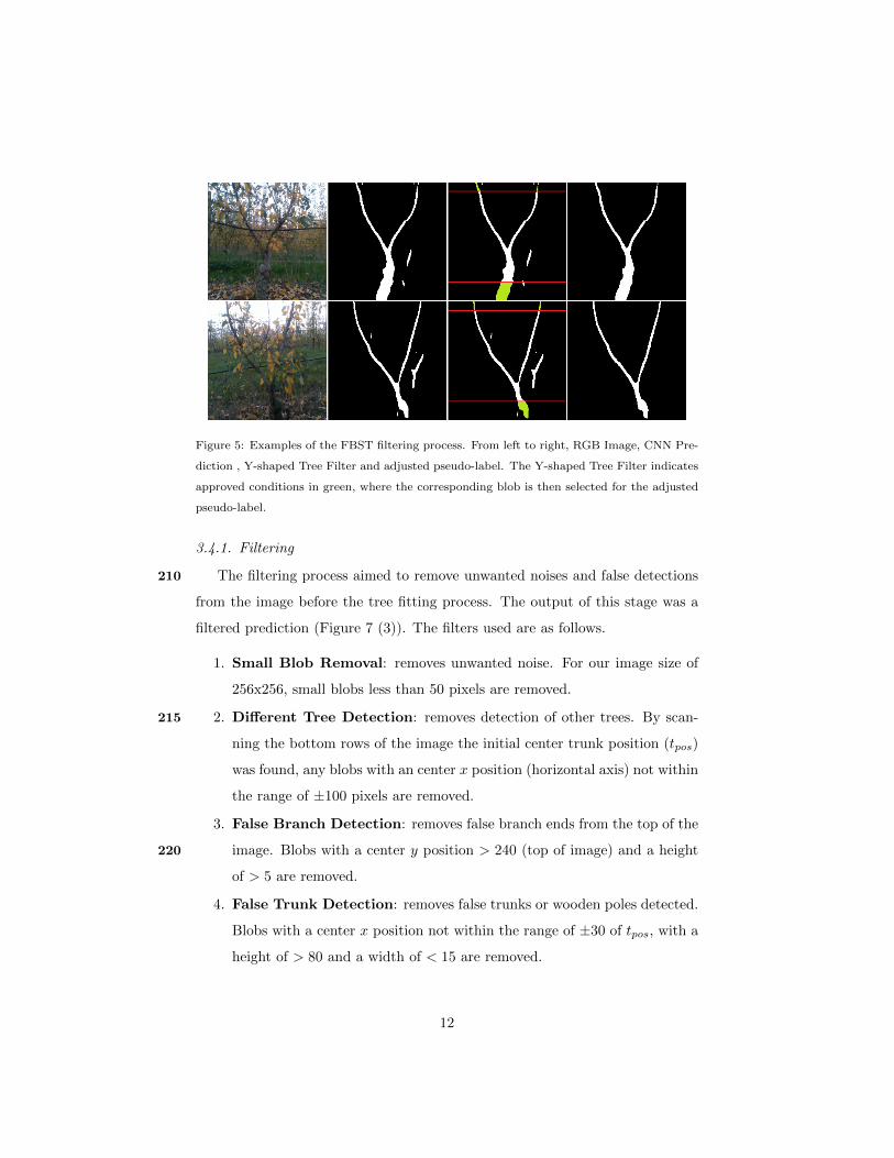
Figure 5: Examples of the FBST filtering process. From left to right, RGB Image, CNN Pre-

diction , Y-shaped Tree Filter and adjusted pseudo-label. The Y-shaped Tree Filter indicates

approved conditions in green, where the corresponding blob is then selected for the adjusted

pseudo-label.

3.4.1. Filtering

The filtering process aimed to remove unwanted noises and false detections210

from the image before the tree fitting process. The output of this stage was a

filtered prediction (Figure 7 (3)). The filters used are as follows.

1. Small Blob Removal: removes unwanted noise. For our image size of

256x256, small blobs less than 50 pixels are removed.

2. Different Tree Detection: removes detection of other trees. By scan-215

ning the bottom rows of the image the initial center trunk position (tpos)

was found, any blobs with an center x position (horizontal axis) not within

the range of ±100 pixels are removed.

3. False Branch Detection: removes false branch ends from the top of the

image. Blobs with a center y position > 240 (top of image) and a height220

of > 5 are removed.

4. False Trunk Detection: removes false trunks or wooden poles detected.

Blobs with a center x position not within the range of ±30 of tpos, with a

height of > 80 and a width of < 15 are removed.

12

3.4.2. Fitting225

The filtering process outputs (filtered predictions) were then given as inputs

to the tree fitting process. This process aimed to fit a tree template, aiming to

generate the missing parts of the tree.

The problem defined for the Genetic Algorithm was to fit a 14-parameter

predefined Y tree template (Figure 6) to a partial tree skeleton. Genetic Algo-230

rithm was selected as the optimization tool as the problem is well defined, but

there are many variables to be optimized. The partial tree skeleton was found

by analyzing each row of the image individually, where each blob was converted

to an average blob position.

The score to be optimized was then calculated using mean absolute error235

(MAE) by comparing the blobs center position in the partial skeleton (Figure

7 (3)) to the generated Y shaped tree template in each row. An example of a

fitted tree template is shown in Figure 7 (4). Compared to other post-processing

methods such as curve fitting, a predefined skeleton can hallucinate portions of

the tree past the endpoint of the partial skeleton.240

A Genetic Algorithm was set up according to the following parameters, we

adopted the notation used for the parameters from Mitchell (1996), Np = 2000,

T = 800, etac = 2, etam = 2, Pc = 0.8 and Pm = 0.5.

The 14 parameters used to define the Y tree template were as follows. Firstly,

to define the trunk there were 4 parameters:245

• (Tpx, 0) = starting point

• (Cp0x, Cp0y) = endpoint of the trunk

• Tpv = gradient of the trunk from the point (Tpx, 0)

Using these boundary conditions, the coefficients of a quadratic curve were

calculated for the trunk.250

To define each branch (i = 1, 2) there were 5 parameters:

• (Cp0x, Cp0y) = starting point

13

• Cpbiv = gradient of the branch from (Cp0x, Cp0y)

• (bip1x, bip1y) = via point of the branch

• (bip2x, 256) = endpoint of the branch255

• bivf = final gradient at the point (bip2x, 256)

Using these boundary conditions the coefficients of a two connected cubic curves

were calculated for each branch. Figure 6 shows an example visual representa-

tion of the 14 parameters that define the Y tree template.

Figure 6: Visual representation of the 14 parameter Y-tree template.

3.4.3. Repairing260

Using the Y-shaped tree template generated from the tree fitting stage, the

horizontal blob thickness profile was measure along the template using the fil-

tered prediction as the reference. Where there are gaps in the thickness profile,

14

the missing thickness values are generated linearly. If an upper endpoint is miss-

ing, a thickness value of 4 pixels is assumed. Additionally, a minimum value of265

generated thickness is set as 3 pixels. These values were selected based on the

average size of the upper endpoints and average minimum branch thicknesses

in the initial training set. A final filter was applied to the image keeping only

the largest blob, finally, the repaired image was generated (Figure 7 (5)).

In this process, images were not used if more than 50% of the branches and270

trunk were reconstructed or if the basic requirements of the basic Y-shaped tree

filter were not met.

Figure 7: Example of each step in the automated process. (1) represents the RGB image; (2)

and (3) are the corresponding CNN Prediction and the Filtered Prediction; (4) is the Fitted

Tree Template fitted to the Filtered Prediction; (5) is the final adjusted and repaired image

and (6) is the ground truth for comparison.

15

3.5. Metrics

3.5.1. Traditional Metrics

To evaluate the performance of the different CNNs and generated labels,275

mean IOU (mIOU) and Boundary F1 (BF1) were used (Csurka and Larlus,

2013; Sasaki, 2007). The 52 images in the validation dataset were used to

evaluate the CNNs. We set the distance threshold to 2 pixels for BF1. In the

application of detecting tree skeletons, where the majority of the image is the

background, mIOU scored relatively close for different quality predictions of the280

same input image. For example, Figure 8 shows an example of a ‘Good’ and

‘Bad’ label, with the RGB and ground truth image for comparison. The metric

values are shown in Table 1. While BF1 score shows a large difference, mIOU

shows relatively small differences in performance.

Additionally, the performance and number of successful labels were analyzed.285

We define a successful label as a completely connected mask with no noise, which

can be used in the environment modeling process.

Figure 8: Example of a successful ’Good’ label (bottom left) and a ’Bad’ label (bottom right)

with the RGB (top left) and ground truth (top right) for comparison.

16

3.5.2. Complete Grid Scan

As mIOU does not accurately reflect the qualitative differences and BF1 fo-

cuses on boundary accuracy, we define an additional metric, the Complete Grid290

Scan (CGS), that reflects the position and thickness accuracy of blobs, and re-

wards good connectivity and low noise. Additionaly, CGS aims to quantitatively

reflect this observed qualitative difference in predictions.

By comparing the prediction to the ground truth, we find the error α, as the

sum of distances between centers and the difference in thickness of each pre-295

diction blob, with the closest ground truth blob measured along the horizontal

rows:

α =

n∑k=1

(|pt(k)− pp(k)|+ |tt(k)− tp(k)|) (1)

where, pt(k) is the center position of the ground truth blob k, pp(k) is the center

position of the closest predicted blob to pt(k), tt(k) is the thickness of the ground

truth blob k and tp(k) is the thickness of the corresponding predicted blob k.300

n is the total number of comparisons.

However, this does not account for a potential difference in the number of

blobs per row. Therefore, we need to consider the total number of errors, ne,

the difference in the number of blobs per row:

ne =

h∑j=1

|nt(j)− np(j)| (2)

where nt(j) is the number of blobs in the ground truth, np(j) is the number of305

blobs in the predicted image, h is the height of image in pixels.

We consider each error in the number of blobs as the maximum possible

distance error in a row, i.e. the image width in pixels, w. Therefore, we defined

η as the error due to incorrect number of blobs:

η = wne (3)

17

We define CGSh as the combination and normalization of the two sources310

of error measured on the horizontal rows.

CGSh = 1− α+ η

w(n+ ne)(4)

CGSv is calculated by repeating the same process measured along the ver-

tical columns, or, by rotating the image 90 degrees and repeating CGSh. The

final CGS is calculated as the average of CGSh and CGSv. An example of CGS

is shown in Figure 9 .315

Figure 9: Example of CGS process, where a single row of a prediction is compared to the

ground truth. The position and thickness of the blobs are compared. Additionally, the blob

error is calculated.

The CGS score for the ‘Good’ and ‘Bad’ image (Figure 8) was calculated

(Table 1). The difference in mIOU performance is small compared to BF1

and CGS, which more accurately reflects the difference in the quality of the

predicted images for this application. CGS performance is an indicator of good

connectivity and low noise.320

18

Table 1: Metric evaluation on the ‘Good’ and ‘Bad’ predictions from Figure 8

mIOU BF1 CGS

Good 0.8028 0.8734 0.9210

Bad 0.7743 0.7561 0.7682

4. Results

All methods (HITL, ATL, FBST, and CST) were evaluated on 52 images

in the validation set. The quality, quantity and effort of each method were

analyzed. The Manual method refers to the CNNs trained on the ground truth

images.325

Two separate trials were completed, each with different initial training set

sizes. In Trial 1, |ST0| = 50 and in Trial 2, |ST0| = 20. In each trial, the

number of new images introduced each iteration was equal to the initial training

set size, excluding the FBST where all unlabeled images were introduced in the

first iteration.330

4.1. Trial 1 - Initial Set Size of 50

Figure 10 shows the performance of the CNNs on the validation dataset for

each method, evaluated over the iterative process. The HITL method performed

relatively close to the manual method across all metrics. The ATL method

achieved comparable performance in the CGS metric, scoring 2.78% lower than335

the manual method, compared to the CST method scoring 9.47% lower. ATL

shows an improved performance compared to both FBST and CST over the

iterative process.

The FBST method performance showed the majority of improvements over

the first four iterations (+11.58%), where the process terminated after 23 iter-340

ations. Improvements slowed as iterations increased and the number of images

passed through the filter reduced. Feeding the whole pool of unlabeled images

allowed for 20.5% of images to be approved by the filter (successfully labeled) on

19

the first iteration. Thereby reducing the maximum number of unlabeled images

that could be approved on subsequent iterations.345

For both ATL and FBST methods, not all unlabeled images were successfully

labeled when the iterative process terminated. This is a result of the custom

process, which acted as a final filter to the data. To compare successful labels

generated in the CST process, the Y-shaped tree filter was applied to the CST

generated labels, indicated by CST w/ Filter.350

The performance of the successful labels for trial 1 in Tables 2.

Method BF1 mIOU CGS Successful Labels

HITL 0.8996 0.8471 0.9482 400

ATL 0.8465 0.8139 0.9136 386

FBST 0.8522 0.8114 0.9077 307

CST 0.7989 0.7887 0.8461 -

CST w/ Filter 0.8485 0.8112 0.9075 73

Table 2: Successful labeled data performance from Trial 1

The maximum number of unlabeled images to be labeled during the iterative

process was 400. ATL successfully labeled 96.5% of images, while FBST suc-

cessfully labeled 76.8% of images. The CST method labeled all unlabeled data,

however, the performance across all metrics was lower compared to all other355

methods. For CST w/ Filter only 18.25% of images were successfully labeled,

with a similar performance to ATL and FBST.

4.2. Trial 2 - Initial Set Size of 20

In Trial 2, we aimed to reduce the human effort to the limit by minimizing the

initial set size. Performance of all methods for each metric in Trial 2 are shown360

in Figure 11. In Trial 2 the initial CNN (CNN0) showed inferior performances

in all metrics.

For the CST method in Trial 1 we observed good behaviors in the initial

predictions compared to Trial 2, such as low noise. Over the iterations, these

good behaviors were reinforced, resulting in a slow upward trend. Compared to365

20

Figure 10: BF1, CGS and mIOU performance of each method during the iterative process of

Trial 1.

Trial 2, where the prediction set size is smaller, and most predictions displayed

bad behaviors such as increased false detections, increased noise and increased

disconnections compared to Trial 1. These behaviors were reinforced over the

iterations where the performance of CST remained relatively similar over the

iterations.370

By reducing the initial training set size, the benefits of ATL were more

predominant compared to Trial 1. With lower quality initial predictions, ATL

had more potential to improve adjustments and continued to trend upward over

the iterations. When compared to both the CST and manual methods, ATL

showed performance relatively close to the manual and HITL methods in CGS.375

With the lower quality initial prediction dataset, the FBST method struggled

to pass images through the filter after a few iterations, compared to Trial 1.

Indicating the FBST method is heavily dependent on the initial training dataset

size, quality of the initial CNN (CNN0) and total data set size (SU0).

21

Figure 11: BF1, CGS and mIOU performance of each method during the iterative process of

Trial 2.

The performance of the successful labels for Trial 2 is shown in Table 3. ATL380

successfully labeled 94.1% of images, while the FBST method successfully la-

beled only 49.5% images. This shows the advantage of a higher level adjustment

process.

Method BF1 mIOU CGS Successful Labels

HITL 0.8926 0.8441 0.9451 440

ATL 0.7984 0.7849 0.9020 414

FBST 0.8176 0.7827 0.8897 218

CST 0.7073 0.7339 0.7613 -

CST w/ Filter 0.8223 0.8086 0.8992 37

Table 3: Successful labeled data performance from Trial 2

CSF labeled all unlabeled data, the performance across all metrics was lower

compared to all other methods. The majority of the images produced by CST385

22

during both trials were not adequate to be used for environment modeling.

This can be seen in Figure 12. When applying the Y-shaped tree filter to labels

generated in CST, only 8.81% of images were successfully labeled.

Figure 12: Examples of the labeled data from each method. The first column represents

the input RGB image. The remaining columns represent the final label generated for each

method, from left to right, CST, FBST, ATL, HITL and Manual respectively.

By increasing the number of unlabeled images in the overall dataset, we

would expect to observe both ATL and FBST to raise the percentage of suc-390

cessfully labeled images due to increased iterations. This would allow more

opportunities to label unsuccessfully labeled data with improving the perfor-

mance of the iterative CNNs and higher quality predictions.

4.3. Human Effort

Human effort measured in minutes is summarised in Table 4. The approx-395

imate time for the HITL method (including both ST0 and all adjusted labels)

was 441.6 and 363.3 minutes for Trials 1 and 2, respectively. In Trial 2 we

observed a reduction factor of 4.3 using the HITL method for this application.

For all other iterative methods, the only effort was to create the initial

training set, resulting in 175 and 70 minutes for Trial 1 and 2. We observed a400

23

Method/s Trial Human Effort (mins)

Manual - 1575

HITL1 441.6

2 363.3

ATL, FBST, CST1 175

2 70

Table 4: Human effort measured in minutes, for each labeling method.

reduction factor of 22.5 in manual labor for ATL, CST, and FBST methods in

Trial 2.

5. Conclusion

In this paper, we presented an iterative training methodology for using CNNs

to segment tree skeletons. To minimze human effort, we introduced Automating-405

the-Loop, which involves attempting to automatically replicate the adjustment

made by annotators in the HITL process. We introduced a new metric, Com-

plete Grid Scan, to indicate good connectivity and low noise in binary images.

Using ATL, we successfully created a CNN with competitive performance to

the manual and HITL CNNs. It was found that ATL has the greatest ratio of410

performance to labeling effort. For semi-supervised methods (including ATL),

the quality of the custom process greatly impacted on the performance. This

results in an interesting problem of balancing the custom processes to generate

successful labels and minimizing human effort. Future work includes using the

ATL method to label other apple tree structures by exploring other automatic415

processes, using these labels to accurately model the 3D farming environment,

and optimization of the iterative training method.

24

References

Castrejon, L., Kundu, K., Urtasun, R., Fidler, S., 2017. Annotating object

instances with a polygon-rnn.420

Chen, Z., Ting, D., Newbury, R., Chen, C., 2021. Semantic segmentation

for partially occluded apple trees based on deep learning. Computers and

Electronics in Agriculture 181, 105952.

URL https://www.sciencedirect.com/science/article/pii/

S0168169920331574425

Cordts, M., Omran, M., Ramos, S., Rehfeld, T., Enzweiler, M., Benenson, R.,

Franke, U., Roth, S., Schiele, B., 2016. The cityscapes dataset for semantic

urban scene understanding. In: Proc. of the IEEE Conference on Computer

Vision and Pattern Recognition (CVPR).

Csurka, G., Larlus, D., 01 2013. What is a good evaluation measure for semantic430

segmentation? IEEE Trans. Pattern Anal. Mach. Intell. 26.

He, K., Zhang, X., Ren, S., Sun, J., 2015. Deep residual learning for image

recognition. CoRR abs/1512.03385.

Intel, 2019. Computer vision annotation tool: A universal approach to data

annotation.435

Kang, H., Chen, C., 2020. Fruit detection, segmentation and 3d visualisation

of environments in apple orchards. Computers and Electronics in Agriculture

171, 105302.

Lau, S. L. H., Chong, E. K. P., Yang, X., Wang, X., 2020. Automated pavement

crack segmentation using u-net-based convolutional neural network. IEEE440

Access 8, 114892–114899.

Lee, H.-W., Kim, N.-r., Lee, J.-H., Mar 2017. Deep neural network self-training

based on unsupervised learning and dropout. The International Journal of

Fuzzy Logic and Intelligent Systems 17 (1), 1–9.

25

Lin, T.-Y., Maire, M., Belongie, S., Hays, J., Perona, P., Ramanan, D., Dollar,445

P., Zitnick, C., 05 2014. Microsoft coco: Common objects in context.

Majeed, Y., Karkee, M., Zhang, Q., Fu, L., Whiting, M. D., 2020. Determining

grapevine cordon shape for automated green shoot thinning using semantic

segmentation-based deep learning networks. Computers and Electronics in

Agriculture 171, 105308.450

Mitchell, M., 1996. An introduction to genetic algorithms. Complex adaptive

systems. MIT Press, Cambridge, Mass.

Ouali, Y., Hudelot, C., Tami, M., 2020a. An overview of deep semi-supervised

learning.

Ouali, Y., Hudelot, C., Tami, M., 2020b. Semi-supervised semantic segmenta-455

tion with cross-consistency training.

Purkait, P., Zach, C., Reid, I., 2019. Seeing behind things: Extending semantic

segmentation to occluded regions. In: 2019 IEEE/RSJ International Confer-

ence on Intelligent Robots and Systems (IROS). pp. 1998–2005.

Ravanbakhsh, M., Klein, T., Batmanghelich, K., Nabi, M., 2019. Uncertainty-460

driven semantic segmentation through human-machine collaborative learning.

Ronneberger, O., Fischer, P., Brox, T., 2015. U-net: Convolutional networks

for biomedical image segmentation. CoRR abs/1505.04597.

Sasaki, Y., 01 2007. The truth of the f-measure. Teach Tutor Mater.

Shen, C., Roth, H. R., Oda, H., Oda, M., Hayashi, Y., Misawa, K., Mori, K.,465

2018. On the influence of dice loss function in multi-class organ segmentation

of abdominal ct using 3d fully convolutional networks.

Sun, X., Shi, A., Huang, H., Mayer, H., 2020. Bas ˆnet: Boundary-aware semi-

supervised semantic segmentation network for very high resolution remote

sensing images. IEEE journal of selected topics in applied earth observations470

and remote sensing 13, 5398–5413.

26

Tong, S., Chang, E., 2001. Support vector machine active learning for image

retrieval. In: Proceedings of the ninth ACM international conference on mul-

timedia. Vol. 9 of MULTIMEDIA ’01. ACM, pp. 107–118.

Ulku, I., Akagunduz, E., 2020. A survey on deep learning-based architectures475

for semantic segmentation on 2d images.

Xiong, B., Oude Elberink, S., Vosselman, G., 06 2016. Footprint map partition-

ing using airborne laser scanning data. ISPRS Annals of Photogrammetry,

Remote Sensing and Spatial Information Sciences III-3, 241–247.

Yao, X., Feng, X., Han, J., Cheng, G., Guo, L., 2020. Automatic weakly super-480

vised object detection from high spatial resolution remote sensing images via

dynamic curriculum learning. IEEE transactions on geoscience and remote

sensing 59 (1), 675–685.

Zhang, C., Chen, T., 2002. An active learning framework for content-based

information retrieval. IEEE Transactions on Multimedia 4 (2), 260–268.485

Zhu, X., Goldberg, A., 2009. Introduction to Semi-Supervised Learning.

27