HAL Id: hal-00115548https://hal.archives-ouvertes.fr/hal-00115548

Submitted on 21 Nov 2006

HAL is a multi-disciplinary open accessarchive for the deposit and dissemination of sci-entific research documents, whether they are pub-lished or not. The documents may come fromteaching and research institutions in France orabroad, or from public or private research centers.

L’archive ouverte pluridisciplinaire HAL, estdestinée au dépôt et à la diffusion de documentsscientifiques de niveau recherche, publiés ou non,émanant des établissements d’enseignement et derecherche français ou étrangers, des laboratoirespublics ou privés.

Minimization problems for eigenvalues of the LaplacianAntoine Henrot

To cite this version:Antoine Henrot. Minimization problems for eigenvalues of the Laplacian. Journal of Evolution Equa-tions, Springer Verlag, 2003, 3, pp.443-461. 10.1007/978-3-0348-7924-8_24. hal-00115548

Minimization problems for eigenvalues of the Laplacian ∗

Antoine HENROT

Ecole des Mines and Institut Elie Cartan Nancy,

UMR 7502 CNRS and projet CORIDA, INRIA,

B.P. 239, 54506 Vandoeuvre-les-Nancy, France.

E-mail : henrot@iecn.u-nancy.fr

Abstract

This paper is a survey on classical results and open questions about minimizationproblems concerning the lower eigenvalues of the Laplace operator. After recallingclassical isoperimetric inequalities for the two first eigenvalues, we present recent ad-vances on this topic. In particular, we study the minimization of the second eigenvalueamong plane convex domains. We also discuss the minimization of the third eigen-value. We prove existence of a minimizer. For others eigenvalues, we just give someconjectures. We also consider the case of Neumann, Robin and Stekloff boundaryconditions together with various functions of the eigenvalues.

AMS classification : 49Q10, 35P15, 49J20.keywords : eigenvalues, minimization, isoperimetric inequalities, optimal domain

1 Introduction

Problems linking the shape of a domain to the sequence of its eigenvalues, or some ofthem, are among the most fascinating of mathematical analysis or differential geometry.In particular, problems of minimization of eigenvalues, or combination of eigenvalues,brought about many deep works since the early part of the twentieth century. Actually,this question appeared in the famous book of Lord Rayleigh ”The theory of sound” ( forexample in the edition of 1894). Thanks to some explicit computations and ”physicalevidence”, Lord Rayleigh conjectured that the disk should minimize the first Dirichleteigenvalue λ1 of the Laplacian among every open sets of given measure.

It was indeed in the 1920’s that Faber [21] and Krahn [34] solved simultaneously theRayleigh’s conjecture using a rearrangement technique. This classical proof is given atTheorem 1 of section 3 which is devoted to the first Dirichlet eigenvalue. We will alsodiscuss the case of a multiconnected domain and present some open problems involving

∗A shorter version of this paper appeared in Journal of Evolution Equations, volume 3 (2003), pp.443-461 special issue dedicated to Philippe Benilan

1

the first eigenvalue. For other problems and a complete bibliography, we refer to [2],[41], [42], [50], [59], [60]; this kind of question is often called ”isoperimetric inequalitiesfor eigenvalues” in standard works, see also [6], [38] [48], [49]. In section 4, we investi-gate similar questions for the second eigenvalue. The open set, of given measure, whichminimizes λ2 is the union of two identical balls. This result is generally attributed toP. Szego, as quoted by G. Polya in [47]), but it was already contained (more or less ex-plicitly) in one of the Krahn’s papers, see [35]. In this section, we will also present veryrecent results about the minimization of λ2 among convex plane domains. In section

Figure 1: The ball minimizes λ1 (left); the union of two identical balls minimizes λ2 (right).

5, we look at the remaining eigenvalues of the Dirichlet-Laplacian. Actually a very fewthings are known! We only know the existence of an optimal domain for λ3 and the factthat this domain is connected in dimension 2 and 3. In section 6, we will consider theso-called ”Payne-Polya-Weinberger” conjecture, solved by Ashbaugh and Benguria in the

90’s, concerning the ratio of the two first eigenvaluesλ2

λ1. We will also present some open

problems on other ratios. Finally, in section 7, we will present some results about otherboundary conditions: Neumann, Robin and also the Stekloff problem. We have decidedhere to restrict ourselves to the Laplacian operator on open (Euclidean) sets. Now, thereare also beautiful results and conjectures e.g. for the bi-Laplacian ∆(∆). A good overviewis given by B. Kawohl in the book [32], see also [37] and [5]. There are also many similarresults on manifolds, see e.g. [39] or [60].

2 Notations and prerequisites

For the basic facts we recall here, we refer to any textbook on partial differential equations.For example, [17] or [20] are good standard references. Let Ω be a bounded open set inR

N . In the case of Dirichlet boundary conditions, the convenient functional space is theSobolev space H1

0 (Ω) which is defined as the closure of C∞ functions compactly supported

in Ω for the norm ‖u‖H1 :=(∫

Ω u(x)2 dx +∫

Ω |∇u(x)|2 dx)1/2

. The Laplacian on Ω withDirichlet boundary conditions is a self-adjoint operator with compact inverse, so thereexists a sequence of positive eigenvalues (going to +∞) and a sequence of correspondingeigenfunctions that we will denote respectively 0 < λ1(Ω) ≤ λ2(Ω) ≤ λ3(Ω) ≤ . . . and

2

u1, u2, u3, . . .. In other words, we have:

−∆uk = λk(Ω)uk in Ωuk = 0 on ∂Ω

(1)

We decide to normalize the eigenfunctions by the condition∫

Ωuk(x)2 dx = 1 . (2)

The sequence of eigenfunctions defines an Hilbert basis of L2(Ω). By hypo-analyticity ofthe Laplacian, each eigenfunction is analytic inside Ω, its behavior on the boundary isgoverned by classical regularity results for elliptic partial differential equations. From themaximum principle and the Krein-Rutman Theorem, it follows that the first eigenfunctionu1 is non negative in Ω and positive as soon as Ω is connected. In particular, since u2 isorthogonal to u1, it has to change the sign in Ω. The sets

Ω+ = x ∈ Ω, u2(x) > 0 and Ω− = x ∈ Ω, u2(x) < 0

are called the nodal domains of u2. According to the Courant-Hilbert Theorem, these twonodal domains are connected subsets of Ω. The set

N = x ∈ Ω, u2(x) = 0

is called the nodal line of u2. When Ω is a plane convex domain, this nodal line hitsthe boundary of Ω at exactly two points, see Melas [36], or Alessandrini [1]. For generalsimply connected plane domains Ω, it is still a conjecture, named after Larry Payne,the ”Payne conjecture”. We will also use the classical variational characterization ofeigenvalues (Poincare principle):

λk(Ω) = minEk ⊂ H1

0 (Ω),subspace of dim k

maxv∈Ek,v 6=0

∫

Ω |∇v(x)|2 dx∫

Ω v(x)2 dx. (3)

This principle implies the following monotonicity for inclusion:

Ω1 ⊂ Ω2 =⇒ λk(Ω1) ≥ λk(Ω2) .

For the first eigenvalue, it reads

λ1(Ω) = infv∈H1

0(Ω),v 6=0

∫

Ω |∇v(x)|2 dx∫

Ω v(x)2 dx(4)

the above infimum being achieved by the first eigenfunction. At last, the eigenvalueshave a simple behavior with respect to homothety: if tΩ denotes the image of Ω by anhomothety with ratio t, the eigenvalues of tΩ satisfy:

λk(tΩ) =λk(Ω)

t2.

3

As a consequence, in two-dimensions, looking for the minimizer of λk(Ω) with a volumeconstraint is equivalent to look for a minimizer of the product |Ω|λk(Ω).

In the sequel, we are interested in minimization problems like

minλk(Ω), Ω open subset of RN , |Ω| = A

(where |Ω| denotes the measure of Ω and A is a given constant). Sometimes, we will alsoconsider other geometric or topologic constraints, this will be specified below.

3 The first eigenvalue of the Dirichlet-Laplacian

3.1 The Rayleigh-Faber-Krahn inequality

For the first eigenvalue, the basic result is (as conjectured by Lord Rayleigh):

Theorem 1 (Rayleigh-Faber-Krahn) Let Ω be any bounded open set in RN , let us

denote by λ1(Ω) its first eigenvalue for the Laplace operator with Dirichlet boundary con-ditions. Let B be the ball of the same volume as Ω, then

λ1(B) = minλ1(Ω), Ω open subset of RN , |Ω| = |B|.

Proof : The classical proof makes use of the Schwarz spherical decreasing rear-rangement. For every bounded open set ω, let ω∗ denotes the ball (centered at theorigin) with the same volume as ω. If u is a non negative function in Ω which vanishes on∂Ω, its spherical decreasing rearrangement is defined as the function u∗ on B = Ω∗ whichhas the following level sets:

∀c > 0, x ∈ B, u∗(x) > c = x ∈ Ω, u(x) > c∗ .

In other words, the level sets of u∗ are the balls that we obtain by rearranging the sets ofsame level of u. We have a first easy consequence (by equi-measurability of the functionsu and u∗):

∫

Bu∗(x)2 dx =

∫

Ωu(x)2 dx . (5)

The following inequality involving the Dirichlet integrals of u and u∗ is much harder toprove, but it is one of the main interest of the rearrangement techniques, we refer to [48]or [6] for the proof:

∫

B|∇u∗(x)|2 dx ≤

∫

Ω|∇u(x)|2 dx . (6)

We can now apply (5) and (6) by choosing for the function u the first eigenfunction u1 ofΩ, it comes:

λ1(Ω) =

∫

Ω |∇u1(x)|2 dx∫

Ω u1(x)2 dx≥

∫

B |∇u∗1(x)|2 dx

∫

B u∗1(x)2 dx

≥ λ1(B)

the last inequality coming from (4), which yields the desired result. ¤

4

3.2 The case of polygons

We can ask the same question for the class of polygons with a given number n of sides.Actually, the result is known only for n = 3 and n = 4:

Theorem 2 (Polya) The equilateral triangle has the least first eigenvalue among all tri-angles of given area. The square has the least first eigenvalue among all quadrilaterals ofgiven area.

The proof relies on the same technique as the Rayleigh-Faber-Krahn Theorem with thedifference that is now used the so-called Steiner symmetrization (see e.g. [48] or [31]).This symmetrization is performed with respect to an hyperplane H: we transform a givenset ω in a set ω∗ symmetric w.r.t H by moving the center of each segment of ω orthogonalto H on H. Doing the same for the level set of a function allows to define the Steinersymmetrization of a given function. This symmetrization has the same properties (5) and(6) as the Schwarz rearrangement, therefore any Steiner symmetrization decreases the firsteigenvalue.

By a sequence of Steiner symmetrization with respect to the mediator of each side, agiven triangle converges to an equilateral one. We can do the same for a quadrilateral byalterning symmetrization w.r.t. mediator of sides and diagonals. It will be transformedinto a square with the means of an infinite sequence of Steiner symmetrization. This isthe idea of Polya’s proof.

Unfortunately, for n ≥ 5 (pentagons and others), the Steiner symmetrization increases, ingeneral, the number of sides. This prevents us to use the same technique. So a beautiful(and hard) challenge is to solve the

Open problem 1 Prove that the regular n-gone has the least first eigenvalue among allthe n-gone of given area for n ≥ 5.

This conjecture is supported by the classical isoperimetric inequality linking area andlength for regular n-gones, see e.g. Theorem 5.1 in Osserman, [38]. Another kind of resultthat can be proved on polygons has been stated by J. Hersch in [28]:Among all parallelograms with given distances between their opposite sides, the rectanglemaximizes λ1.

3.3 Domains in a box

Instead of looking at open sets just with a given volume, we could consider open setsconstrained to lie into a given box D (and also with a given volume). In other words, wecould look for the solution of

minλ1(Ω), Ω ⊂ D, |Ω| = A (given). (7)

According to the Theorem 7 of Buttazzo-DalMaso which will be stated below, the problem(7) has always a solution. Of course, if the constant A is small enough in such a way

5

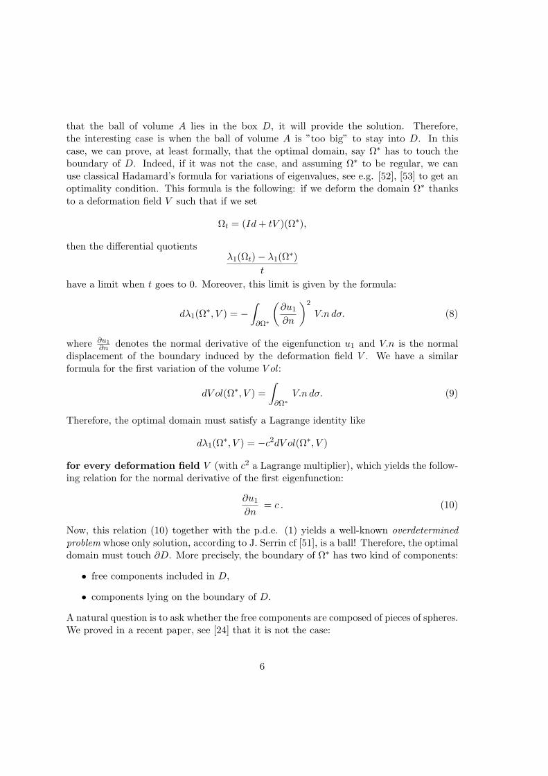
that the ball of volume A lies in the box D, it will provide the solution. Therefore,the interesting case is when the ball of volume A is ”too big” to stay into D. In thiscase, we can prove, at least formally, that the optimal domain, say Ω∗ has to touch theboundary of D. Indeed, if it was not the case, and assuming Ω∗ to be regular, we canuse classical Hadamard’s formula for variations of eigenvalues, see e.g. [52], [53] to get anoptimality condition. This formula is the following: if we deform the domain Ω∗ thanksto a deformation field V such that if we set

Ωt = (Id + tV )(Ω∗),

then the differential quotientsλ1(Ωt) − λ1(Ω

∗)

t

have a limit when t goes to 0. Moreover, this limit is given by the formula:

dλ1(Ω∗, V ) = −

∫

∂Ω∗

(

∂u1

∂n

)2

V.n dσ. (8)

where ∂u1

∂n denotes the normal derivative of the eigenfunction u1 and V.n is the normaldisplacement of the boundary induced by the deformation field V . We have a similarformula for the first variation of the volume V ol:

dV ol(Ω∗, V ) =

∫

∂Ω∗

V.n dσ. (9)

Therefore, the optimal domain must satisfy a Lagrange identity like

dλ1(Ω∗, V ) = −c2dV ol(Ω∗, V )

for every deformation field V (with c2 a Lagrange multiplier), which yields the follow-ing relation for the normal derivative of the first eigenfunction:

∂u1

∂n= c . (10)

Now, this relation (10) together with the p.d.e. (1) yields a well-known overdeterminedproblem whose only solution, according to J. Serrin cf [51], is a ball! Therefore, the optimaldomain must touch ∂D. More precisely, the boundary of Ω∗ has two kind of components:

• free components included in D,

• components lying on the boundary of D.

A natural question is to ask whether the free components are composed of pieces of spheres.We proved in a recent paper, see [24] that it is not the case:

6

D

Ω*

Figure 2: Ω∗ solves the problem (7): the free components of ∂Ω∗ are not arc of circles.

Proposition 2.1 The free components of the domain Ω∗ which solve problem (7) cannotbe pieces of spheres unless the ball of volume A is the solution.

Proof : Let us assume that ∂Ω∗ contains a piece of sphere γ. On γ, Ω∗ satisfies theoptimality condition (10). We put the origin at the center of the corresponding ball andwe introduce the functions

wi,j(x, y) = xi∂u

∂xj− xj

∂u

∂xi.

Then, we easily verify that−∆wi,j = λ1wi,j in Ω∗

wi,j = 0 in γ∂wi,j

∂n = 0 in γ.

Now we conclude, using Holmgren uniqueness theorem, that wi,j must vanish in a neigh-borhood of γ, so in the whole domain by analyticity. Now, if all these functions wi,j areidentically 0 in Ω∗, this would imply that u is radially symmetric in Ω∗ and therefore thatΩ∗ is a ball. ¤

Nevertheless, there are some interesting open questions for this very simple minimizationproblem. For example:

Open problem 2 Let Ω∗ be a solution of the minimization problem (7). Prove that thefree components of the boundary of Ω∗ are C∞ (or analytic). If D is convex, is ittrue that Ω∗ is convex?

3.4 Multi-connected domains

This section could also be entitled ”How to place an obstacle” (see [23]). Let us considera multi-connected domain Ω with one or several holes whose boundaries are denoted byΓ0, Γ1, . . ., the outer boundary of Ω being denoted by Γ. We can consider many problems,letting the boundary conditions varying on the outer boundary and/or the holes. Let me

7

mention below the results known by the author on such minimization and maximizationproblems.

• One hole, Dirichlet boundary condition on Γ and Γ0. J. Hersch in [27] proves:Of all such plane domains, with given area A, and given length L and L0 of its outerand inner boundary satisfying L2 − L2

0 = 4πA, the annular domain (two concentriccircles) maximizes λ1.This result implies, in particular, that for a domain Ω of the kind Ω = B1\B0 (differ-ence of two disks of given radii), λ1 is maximal when the disks are concentric. Thisparticular result has been rediscovered later and extended to the N -dimensional caseby several authors: M. Ashbaugh and T. Chatelain in 1997 (private communication),E. Harrel, P. Kroger and K. Kurata in [23], Kesavan, see [33]. They also proved thatλ1(B1 \ B0) is a minimum when B0 touches the boundary of B1.

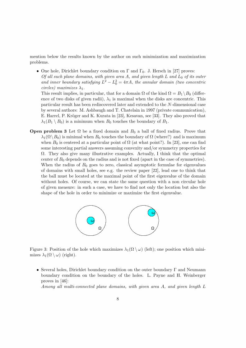
Open problem 3 Let Ω be a fixed domain and B0 a ball of fixed radius. Prove thatλ1(Ω\B0) is minimal when B0 touches the boundary of Ω (where?) and is maximumwhen B0 is centered at a particular point of Ω (at what point?). In [23], one can findsome interesting partial answers assuming convexity and/or symmetry properties forΩ. They also give many illustrative examples. Actually, I think that the optimalcenter of B0 depends on the radius and is not fixed (apart in the case of symmetries).When the radius of B0 goes to zero, classical asymptotic formulae for eigenvaluesof domains with small holes, see e.g. the review paper [22], lead one to think thatthe ball must be located at the maximal point of the first eigenvalue of the domainwithout holes. Of course, we can state the same question with a non circular holeof given measure: in such a case, we have to find not only the location but also theshape of the hole in order to minimize or maximize the first eigenvalue.

Ω Ω

ω

ω

Figure 3: Position of the hole which maximizes λ1(Ω \ ω) (left); one position which mini-mizes λ1(Ω \ ω) (right).

• Several holes, Dirichlet boundary condition on the outer boundary Γ and Neumannboundary condition on the boundary of the holes. L. Payne and H. Weinbergerproves in [46]:Among all multi-connected plane domains, with given area A, and given length L

8

of its outer boundary, the annular domain (two concentric circles) maximizes thefirst eigenvalue λ1 with Dirichlet boundary condition on the outer boundary Γ andNeumann boundary condition on the boundary of the holes.

• Several holes, Neumann boundary condition on the outer boundary Γ, Dirichletboundary condition on one hole and Neumann boundary condition on the boundaryof the other holes. J. Hersch proves in [27]:Among all multi-connected plane domains, with given area A, and given length L0

of the first inner boundary, the annular domain (two concentric circles) maximizesthe first eigenvalue λ1 with Neumann boundary condition on the outer boundary Γ,Dirichlet boundary condition on one hole and Neumann boundary condition on theboundary of the other holes.

4 The second eigenvalue of the Dirichlet-Laplacian

For the second eigenvalue, the minimizer is not one ball, but two!

Theorem 3 (Krahn-Szego) The minimum of λ2(Ω) among bounded open sets of RN

with given volume is achieved by the union of two identical balls.

Proof : Let Ω be any bounded open set, and let us denote by Ω+ and Ω− its nodaldomains. Since u2 satisfies

−∆u2 = λ2u2 in Ω+

u2 = 0 on ∂Ω+

λ2(Ω) is an eigenvalue for Ω+. But, since u2 is positive in Ω+, it is the first eigenvalue(and similarly for Ω−):

λ1(Ω+) = λ1(Ω−) = λ2(Ω) . (11)

We now introduce Ω∗+ and Ω∗

− the balls of same volume as Ω+ and Ω− respectively.According to the Rayleigh-Faber-Krahn inequality

λ1(Ω∗+) ≤ λ1(Ω+), λ1(Ω

∗−) ≤ λ1(Ω−) . (12)

Let us introduce a new open set Ω defined as

Ω = Ω∗+ ∪ Ω∗

− .

Since Ω is disconnected, we obtain its eigenvalues by gathering and reordering the eigen-values of Ω∗

+ and Ω∗−. Therefore,

λ2(Ω) ≤ max(λ1(Ω∗+), λ1(Ω

∗−)) .

According to (11), (12) we have

λ2(Ω) ≤ max(λ1(Ω+), λ1(Ω−)) = λ2(Ω) .

9

This shows that the minimum of λ2 is to be obtained among the union of balls. But,if the two balls would have different radii, we would decrease the second eigenvalue byshrinking the largest one and dilating the smaller one (without changing the total volume).Therefore, the minimum is achieved by the union of two identical balls. ¤

Being disappointed that the minimizer be not a connected set (it’s hard to hit withone hand on a non-connected drum!), we could be interested in solving the minimizationproblem for λ2 among connected sets. Unfortunately, a connectedness constraint doesnot really change the situation. Indeed, let us consider the following domain (see Figure4) Ωε, obtained by joining the union of the two previous balls Ω by a thin pipe of widthε. We say that Ωε γ-converges to Ω if the resolvent operators Tε associated with the

Ωε

Figure 4: A minimizing sequence of connected domains (left), the stadium does not mini-mize λ2 among convex sets of given volume (right)

Laplace-Dirichlet operator on Ωε simply converge to the corresponding operator T on Ω,see e.g. [18]. By a compactness argument, see [12], [26] it can be proved that this simpleconvergence implies the convergence in the operator norm and therefore the convergenceof the eigenvalues. Now, it is easy to verify, see [11], [26], that in the above situation Ωε

γ-converges to Ω what yields λ2(Ωε) → λ2(Ω) and therefore:

infλ2(Ω), Ω ⊂ RN , Ω connected , |Ω| = c = minλ2(Ω), Ω ⊂ R

N , |Ω| = c

what shows that this infimum is not achieved (actually, we can prove that the union oftwo balls is the unique minimizer of λ2 up to displacements and zero-capacity subsets).

Now, the problem becomes again interesting if we ask the question to find the convexdomain, of given area, which minimizes λ2. For sake of simplicity, we restrict us here tothe two-dimensional case. Existence of a minimizer Ω∗ is easy to obtain (see [15] and [24],[25]). In a paper of 1973 [55], Troesch did some numerical experiments which led him toconjecture that the solution was a stadium: the convex hull of two identical tangent disks.It is actually the convex domain which is the closest to the solution without convexityconstraint. In [24], we refute this conjecture:

Theorem 4 (Henrot-Oudet) The stadium, convex hull of two identical tangent disks,does not realize the minimum of λ2 among plane convex domains of given area.

Indeed, the proof is exactly the same as the proof of the above Proposition 2.1. Never-theless, a more precise analysis and some numerical experiments show that the minimizer,say Ω∗, is very close to the stadium. Actually, we prove in [24], [25]:

10

Theorem 5 (Henrot-Oudet)

Regularity The minimizer Ω∗ is at least C1 and at most C2.

Simplicity The second eigenvalue of Ω∗ is simple.

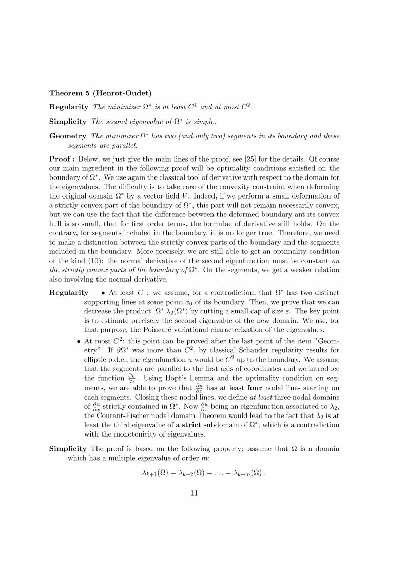
Geometry The minimizer Ω∗ has two (and only two) segments in its boundary and thesesegments are parallel.

Proof : Below, we just give the main lines of the proof, see [25] for the details. Of courseour main ingredient in the following proof will be optimality conditions satisfied on theboundary of Ω∗. We use again the classical tool of derivative with respect to the domain forthe eigenvalues. The difficulty is to take care of the convexity constraint when deformingthe original domain Ω∗ by a vector field V . Indeed, if we perform a small deformation ofa strictly convex part of the boundary of Ω∗, this part will not remain necessarily convex,but we can use the fact that the difference between the deformed boundary ant its convexhull is so small, that for first order terms, the formulae of derivative still holds. On thecontrary, for segments included in the boundary, it is no longer true. Therefore, we needto make a distinction between the strictly convex parts of the boundary and the segmentsincluded in the boundary. More precisely, we are still able to get an optimality conditionof the kind (10): the normal derivative of the second eigenfunction must be constant onthe strictly convex parts of the boundary of Ω∗. On the segments, we get a weaker relationalso involving the normal derivative.

Regularity • At least C1: we assume, for a contradiction, that Ω∗ has two distinctsupporting lines at some point x0 of its boundary. Then, we prove that we candecrease the product |Ω∗|λ2(Ω

∗) by cutting a small cap of size ε. The key pointis to estimate precisely the second eigenvalue of the new domain. We use, forthat purpose, the Poincare variational characterization of the eigenvalues.

• At most C2: this point can be proved after the last point of the item ”Geom-etry”. If ∂Ω∗ was more than C2, by classical Schauder regularity results forelliptic p.d.e., the eigenfunction u would be C2 up to the boundary. We assumethat the segments are parallel to the first axis of coordinates and we introducethe function ∂u

∂x . Using Hopf’s Lemma and the optimality condition on seg-

ments, we are able to prove that ∂u∂x has at least four nodal lines starting on

each segments. Closing these nodal lines, we define at least three nodal domainsof ∂u

∂x strictly contained in Ω∗. Now ∂u∂x being an eigenfunction associated to λ2,

the Courant-Fischer nodal domain Theorem would lead to the fact that λ2 is atleast the third eigenvalue of a strict subdomain of Ω∗, which is a contradictionwith the monotonicity of eigenvalues.

Simplicity The proof is based on the following property: assume that Ω is a domainwhich has a multiple eigenvalue of order m:

λk+1(Ω) = λk+2(Ω) = . . . = λk+m(Ω) .

11

Then, we can always find a deformation field V ∈ C1,1(RN , RN ), preserving thevolume and such that, if we set

Ωt = (Id + tV )(Ω)

we have, for t > 0 small enough

λk+1(Ωt) < λk+1(Ω) = λk+m(Ω) < λk+m(Ωt) .

The proof of this fact uses computations of the domain derivative for multiple eigen-values. The previous result has the following consequence about minimization ofeigenvalues: if Ω∗ is a domain minimizing the k-th eigenvalue and if λk(Ω

∗) is notsimple, necessarily we have

λk−1(Ω∗) = λk(Ω

∗). (13)

Actually, numerical experiments show that this relation holds in every case, see [40]:the domain which minimizes λk(Ω) , k ≥ 2 (with a volume constraint but withoutconvexity constraint) always satisfies (13). Coming back to a convex domain Ω∗

minimizing λ2, we know that λ1(Ω∗) is simple and therefore (13) cannot hold.

Geometry • There is at least one segment on the boundary, otherwise the normalderivative of u would be zero on the whole boundary, because it is constant(by optimality condition) and it has to be zero where the nodal line hits theboundary. It is easy to see that it is impossible, e.g. using one more timeHolmgren uniqueness argument.

• There are at least two segments on the boundary, otherwise the nodal linewould have to close on the same segment and we could adapt an idea of Melas[36] to reach a contradiction.

• There are at most two segments on the boundary, otherwise we consider thesegment S in the boundary which does not meet the nodal line. We put ithorizontal and we introduce the auxiliary eigenfunction vt = tu + ∂u

∂x . Thanksto the optimality condition on segments, we prove that this function has at leastthree nodal lines starting on S for t small. Then, we reach a contradiction byletting t increasing up to a critical value where vt would have all its derivativeswhich vanish up to the second order at some point and therefore everywhere.

• The two segments have to be parallel. To see that, we use some Rellich-Pucci-Serrin formulae for a well-chosen vector field together with the optimality con-ditions. This allow us to prove that the angle between the two segments has tovanish. ¤

Open problem 4 Prove that a plane convex domain Ω∗ which minimizes λ2 (amongconvex domains of given area) has two perpendicular axes of symmetry.

12

5 Other eigenvalues of the Dirichlet-Laplacian

The minimization problem becomes much more complicated for the other eigenvalues!One of the only known result is the following, cf [10] and [58]:

Theorem 6 (Bucur-Henrot and Wolff-Keller) There exists a set Ω∗3 which minimizes

λ3 among the (quasi)-open sets of given volume. Moreover Ω∗3 is connected in dimension

N =2 or 3.

The question of identifying the optimal domain Ω∗3 remains open. The conjecture is the

following:

Open problem 5 Prove that the optimal domain for λ3 is a ball in dimension 2 and 3and the union of three identical balls in dimension N ≥ 4.

Wolff and Keller have proved in [58] that the disk is a local minimizer for λ3. There aretwo key-points in the existence proof of the above theorem. The first one is a more generalresult of Buttazzo-Dal Maso (already cited earlier), see [12]:

Theorem 7 (Buttazzo-Dal Maso) Let D be a fixed ball in RN . For every fixed integer

k ≥ 1 and c fixed real number 0 < c < |D| the problem

minλk(Ω); Ω ⊂ D, |Ω| = c (14)

has a solution.More generally, the existence result remains valid for any function Φ(λ1, . . . , λk) of theeigenvalues non decreasing in each of its arguments.

This theorem does not solve the general problem of existence of a minimizer for λk(Ω)since we assume to work with ”confined” sets (that is to say, sets included in a box D). Inorder to remove this assumption in [10], we used a ”concentration-compactness” argumenttogether with the Wolff-Keller’s result proving that the minimizer of λ3 (if it exists) shouldbe connected in dimension 2 and 3 (this is the second key-point). Here is the more generalresult they prove in [58]. Let us denote by Ω∗

n an open set which minimizes λn (amongopen sets of volume 1) and λ∗

n = λn(Ω∗n) the minimal value of λn. We will also denote by

tΩ the image of Ω by an homothety of ratio t. Then, we have:

Theorem 8 (Wolf-Keller) Let us assume that Ω∗n is the union of (at least) two disjoints

sets, each of them with positive measure. Then

(λ∗n)N/2 = (λ∗

i )N/2 +

(

λ∗n−i

)N/2= min

1≤j≤(n−1)/2((

λ∗j

)N/2+

(

λ∗n−j

)N/2) (15)

where, in the previous equality, i is a value of j ≤ (n − 1)/2 which minimizes the sum(

λ∗j

)N/2+

(

λ∗n−j

)N/2. Moreover,

Ω∗n =

[

(

λ∗i

λ∗n

)1/2

Ω∗i

]

⋃

[

(

λ∗n−i

λ∗n

)1/2

Ω∗n−i

]

. (16)

13

We have seen that the value of λ∗n is not known unless for n = 1 or 2. Let us prove

for example, that the optimal domain is connected in dimension 2. Indeed, if it was notconnected, according to Theorem 8, we should have λ∗

3 = λ∗1 + λ∗

2 (i = 1 is the onlypossible value here). Now λ∗

1 = πj20,1 = 18.168.. (j0,1 is the first zero of the Bessel function

J0) while, according to Theorem 3, λ∗2 = 2λ∗

1 = 36.336. Therefore λ∗1 + λ∗

2 = 54.504.But since λ∗

3 is, by definition, lower or equal to the third eigenvalue of the unit diskλ3(D1) = πj2

1,1 = 46.125.., we see that it cannot be equal to λ∗1 + λ∗

2.The same kind of computation works in dimension 3, but not in higher dimension.

This is the reason why we think that the minimizer is the union of three identical ballsin dimension greater than 4. To prove that the disk is a local minimizer of λ3, Wolffand Keller use some precise perturbation argument. More precisely, they show that thethird eigenvalue of a domain Ωε given in polar coordinates by r = R(θ, ε) where R has anexpansion like

R(θ, ε) = 1 + ε∞

∑

n=−∞

aneinθ + ε2∞

∑

n=−∞

bneinθ + O(ε3) (17)

is given byλ3(Ωε) = πj2

1,1(1 + 2|ε||a2|) + O(ε2).

In the case where a2 6= 0, we immediately get the result. When a2 = 0 it is necessary tolook at the following term in the expansion, but the conclusion is the same. For the fourth

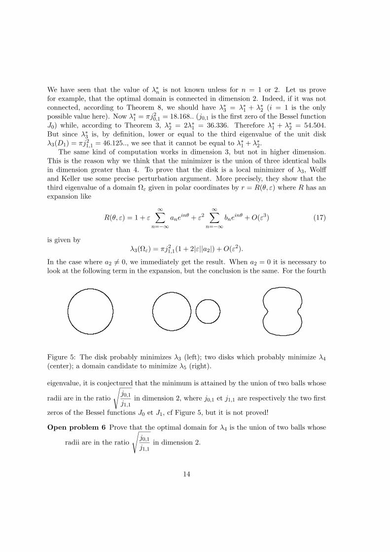
Figure 5: The disk probably minimizes λ3 (left); two disks which probably minimize λ4

(center); a domain candidate to minimize λ5 (right).

eigenvalue, it is conjectured that the minimum is attained by the union of two balls whose

radii are in the ratio

√

j0,1

j1,1in dimension 2, where j0,1 et j1,1 are respectively the two first

zeros of the Bessel functions J0 et J1, cf Figure 5, but it is not proved!

Open problem 6 Prove that the optimal domain for λ4 is the union of two balls whose

radii are in the ratio

√

j0,1

j1,1in dimension 2.

14

Looking at the previous results and conjectures, P. Szego asked the following question:Is it true that the minimizer of any eigenvalue of the Laplace-Dirichlet operator is a ballor a union of balls?The answer to this question is NO. For example, Wolff and Keller remarked that thethirteenth (!) eigenvalue of a square is lower than the thirteenth eigenvalue of any unionof disks of same area. Actually, it is not necessary to go to the 13th eigenvalue. Numericalexperiments, cf [40] and Figure 5, show that for the n-th eigenvalue with n larger or equalto 5 the minimizer is no longer a ball or a union of balls.

Let us state now some new open problems:

Open problem 7 Prove that there exist a minimizer for λn among open sets of givenvolume. The technique we used in [10] allows us to prove such an existence result assoon as we are able to prove that the minimizers for λk, k = 1 . . . n − 1 are indeedbounded.Study the regularity and the geometric properties (e.g. symmetries) of such a mini-mizer.

6 Optimizing functions of eigenvalues

6.1 Maximizing ratios of eigenvalues

In 1955 L. Payne, G. Polya and H. Weinberger in [43] considered the problem of bounding

ratios of eigenvalues. In particular, they proved that the ratioλ2

λ1is less than or equal to

3 (in dimension 2). They were led to conjecture that the optimal domain for this ratio isa disk. This conjecture has been proved 35 years later by M. Ashbaugh and R. Benguria,see [3] for the two-dimensional case and [4] for the N -dimensional case.

Theorem 9 (Ashbaugh-Benguria) The ball maximizes the ratioλ2

λ1.

Their (clever) proof uses

• a variational characterization for the difference λ2 − λ1,

• the Brouwer fixed point theorem,

• a sharp use of some rearrangement inequalities,

• another inequality due to Chiti,

• a careful study of properties of Bessel functions.

For ratios of eigenvalues, many problems remain open. A good overview and discussionon previous results is given in [2]. Below, some of them are listed

15

Open problem 8 (see [43]) Prove that the disk maximizes the quotientλ2 + λ3

λ1among

plane domains of given area.

Prove that the ball maximizes the quotient

∑N+1i=2 λi

λ1among domains of R

N with

given area.

Open problem 9 Prove existence of a domain which maximizes the following ratios,study the geometric properties of such maximizers, if possible identify it

•λ3

λ1(in the plane this is not the disk)

•λN+2

λ1in R

N : it should be the ball

•λm+1

λm

•λ2m

λm

6.2 Other functions of eigenvalues

We have already mentioned in Theorem 7 that any function of the kind Ω 7→ Φ(λ1(Ω), λ2(Ω))with Φ non decreasing with respect to each argument, admits a minimizer among (quasi)-open sets of given volume. Note than none of the above ratios can be handled by thistheorem. In an interesting paper [9], D. Bucur, G. Buttazzo and I.Figueiredo extendedthis result:

Theorem 10 (Bucur, Buttazzo, Figueiredo) Let Φ : R2→ R be a lower semi-continu-

ous function, D a given box and A a given constant. Then the problem

minΦ(λ1(Ω), λ2(Ω)), Ω ⊂ D, |Ω| ≤ A

has always a solution.

A more precise statement could be: either an optimal domain exists or for the minimizingsequence Ωn we have Φ(λ1(Ωn), λ2(Ωn)) → −∞. In this last case, we can choose as aminimizer the empty set. This is the case, for example for the gap function Φ(λ1, λ2) =λ1 − λ2. Indeed, if we consider a sequence of domains

Ωε = B(0, ε) ∪Nε

i=1 B(xi, aεε)

where aε < 1 and Nε are chosen such that |Ωε| = A and λi(Ωε) = λi(B(0, ε)) for i = 1, 2,then

λ1(Ωε) − λ2(Ωε) → −∞.

The main ingredient of the proof of this theorem is the closedness (in the plane) of the set

16

λ1

λ2

λ2=λ

1

λ2=2.53..λ

1

A

B

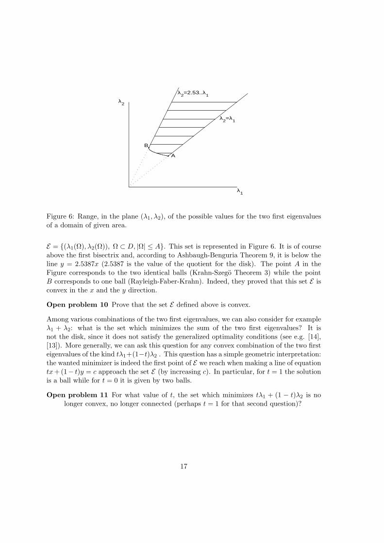
Figure 6: Range, in the plane (λ1, λ2), of the possible values for the two first eigenvaluesof a domain of given area.

E = (λ1(Ω), λ2(Ω)), Ω ⊂ D, |Ω| ≤ A. This set is represented in Figure 6. It is of courseabove the first bisectrix and, according to Ashbaugh-Benguria Theorem 9, it is below theline y = 2.5387x (2.5387 is the value of the quotient for the disk). The point A in theFigure corresponds to the two identical balls (Krahn-Szego Theorem 3) while the pointB corresponds to one ball (Rayleigh-Faber-Krahn). Indeed, they proved that this set E isconvex in the x and the y direction.

Open problem 10 Prove that the set E defined above is convex.

Among various combinations of the two first eigenvalues, we can also consider for exampleλ1 + λ2: what is the set which minimizes the sum of the two first eigenvalues? It isnot the disk, since it does not satisfy the generalized optimality conditions (see e.g. [14],[13]). More generally, we can ask this question for any convex combination of the two firsteigenvalues of the kind tλ1+(1−t)λ2 . This question has a simple geometric interpretation:the wanted minimizer is indeed the first point of E we reach when making a line of equationtx+(1− t)y = c approach the set E (by increasing c). In particular, for t = 1 the solutionis a ball while for t = 0 it is given by two balls.

Open problem 11 For what value of t, the set which minimizes tλ1 + (1 − t)λ2 is nolonger convex, no longer connected (perhaps t = 1 for that second question)?

17

7 Eigenvalues of the Laplacian with other boundary condi-

tions

7.1 Neumann boundary conditions

The eigenvalues of the Laplacian with Neumann boundary conditions are also called theeigenvalues of the free membrane (in the case of Dirichlet boundary conditions, we speakabout the fixed membrane). We will denote it by 0 = µ1(Ω) ≤ µ2(Ω) ≤ µ3(Ω) ≤ . . . (thefirst eigenvalue is zero, corresponding to constant functions). They solve

−∆uk = µk(Ω)uk in Ω∂uk

∂n = 0 on ∂Ω .(18)

Minimizing the eigenvalues of the Laplacian with Neumann boundary conditions, with avolume constraint, is a trivial problem. Indeed, if we consider a long thin rectangle like

]0, L[×]0, l[, its n-th eigenvalue will be (for L large enough) µn =(n − 1)2π2

L2. Therefore,

letting L → +∞, we see that

infµn(Ω), |Ω| = A = 0 .

Moreover, the infimum is attained for any open set which has at least n connected com-ponents. This shows that limiting the diameter of Ω does not improve the interest of thequestion! Now, if we assume that the domains must be convex and with a given diameter,then the infimum is not zero, but it is not achieved! Actually, L. Payne and H. Weinbergerproved in [45] the following inequality for convex domains Ω in R

N with given diameter d:

µ2(Ω) ≥(π

d

)2.

This lower bound is optimal but not attained: any domain shrinking to a one-dimensionalsegment [0, d] has its second eigenvalue which converges to the lower bound.

If we want to get a really interesting problem for eigenvalues of the Laplacian with Neu-mann boundary conditions, we must consider the problem of the maximization insteadof the minimization:

Theorem 11 (Szego,Weinberger) The ball maximizes the second Neumann eigenvalueamong open sets of given volume.

In the two-dimensional case, the proof (using conformal maps) was given by G. Szegoin [54]. It has been generalized to any dimension by H. Weinberger in [56]. We mustalso mention that Szego and Weinberger in the above-mentioned papers have proved intwo-dimensions that

1

µ2+

1

µ3is minimal for the disk.

Of course this result implies Theorem 11 since the second eigenvalue of the disk is double.Now, in higher dimensions, it is still an open problem:

18

Open problem 12 Prove thatN+1∑

i=2

1

µi(Ω)

is minimal for the ball among all domains with a given volume.

More generally, the existence of a convex domain which maximizes the n-th Neumanneigenvalue µn (with given volume) has been proved in [16]. So, we are also led to thefollowing open problem(s):

Open problem 13 Prove that there exists an open set (of given volume) which maxi-mizes the n-th Neumann eigenvalue µn, for n ≥ 3. If possible, identify this maxi-mizer.

7.2 Robin boundary condition

The eigenvalues of the Laplacian with Robin boundary conditions are called the eigenvaluesof the elastically supported membrane. We will denote them by 0 < ν1(α,Ω) ≤ ν2(α,Ω) ≤ν3(α,Ω) ≤ . . . where α is a parameter, 0 < α < 1 (the cases α = 0 or 1 obviouslycorrespond to Neumann or Dirichlet conditions). The p.d.e. system is

−∆uk = νk(α,Ω)uk in Ω

αu + (1 − α)∂uk

∂n = 0 on ∂Ω .(19)

In two dimensions, we recover the Rayleigh-Faber-Krahn inequality; this result is not wellknown, it is due to M.H. Bossel in her thesis:

Theorem 12 (Bossel) The disk minimizes the first eigenvalue of the Robin problemamong open sets with a given volume (for every value of α ∈]0, 1]).

Her proof uses a new variational method, see [7]. This method is inspired by that ofextremal length.

Open problem 14 Generalize Bossel’s Theorem to dimension N .

Open problem 15 (see [44]) For what values of α, the ratioλ2

λ1achieves its maximum

for the disk? Let us remark that Problem 14 is already stated in Daners, see [19]where a lower bound for ν1 is given.

7.3 Stekloff eigenvalue problem

The Stekloff eigenvalue problem is the following:

∆u = 0 in Ω∂u∂n = pu on ∂Ω .

(20)

19

We will denote its eigenvalues by 0 = p1(Ω) ≤ p2(Ω) ≤ p3(Ω) ≤ . . . (the first eigenvalue iszero, corresponding to constant functions). Like in the Neumann case, it is the problemof maximization of the eigenvalues which is interesting here.

Theorem 13 (Weinstock,Brock) The ball maximizes the second Stekloff eigenvalueamong open sets of given volume.

R. Weinstock gave the proof of this theorem in the two-dimensional case in [56]. His proofwas inspired by the one of Szego for the free membrane problem. F. Brock in [8] provedactually a sharper inequality, namely:Let Ω be a bounded domain in R

N and R the radius of the ball Ω∗ of same volume thanΩ, then

N+1∑

i=2

1

pi(Ω)≥ NR (21)

the equality sign in (21) is attained if Ω is a ball. It is clear that (21) implies the abovetheorem since p2(Ω

∗) = 1/R has multiplicity N for the ball. I must also mention that J.Hersch and L. Payne have already proved (21) in two-dimensions in [29] and that theyhave also proved a sharper inequality, together with M.M. Schiffer in [30], namely:the disk maximizes the product p2(Ω)p3(Ω) among plane open sets of given volume.

Open problem 16 Study the maximization problem for other Stekloff eigenvalues.

Open problem 17 Prove that the N -ball maximizes the product ΠN+1k=2 pk(Ω) among

open sets in RN with given volume.

References

[1] G. Alessandrini, Nodal lines of eigenfunctions of the fixed membrane problem ingeneral convex domains, Comment. Math. Helv., 69 (1994), no. 1, 142-154.

[2] M.S. Ashbaugh, Open problems on eigenvalues of the Laplacian, Analytic and Ge-ometric Inequalities and Their Applications, T. M. Rassias and H. M. Srivastava(editors), vol. 4787, Kluwer 1999.

[3] M.S. Ashbaugh, R. Benguria, Proof of the Payne-Polya-Weinberger conjecture,Bull. Amer. Math. Soc., 25 no1 (1991), 19–29.

[4] M.S. Ashbaugh, R. Benguria, A sharp bound for the ratio of the first two eigenval-ues of Dirichlet Laplacians and extensions, Ann. of Math. 135 (1992), no. 3, 601-628.

[5] M.S. Ashbaugh, R. Benguria, On Rayleigh’s conjecture for the clamped plate andits generalization to three dimensions, Duke Math. J., 78 (1995), 1-17.

20

[6] C. Bandle Isoperimetric inequalities and applications. Monographs and Studies inMathematics, 7. Pitman, Boston, Mass.-London, 1980.

[7] M.H. Bossel, Membranes elastiquement liees: extension du theoreme de Rayleigh-Faber-Krahn et de l’inegalite de Cheeger, C. R. Acad. Sci. Paris Sr. I Math. 302(1986), no. 1, 47-50.

[8] F. Brock, An isoperimetric inequality for eigenvalues of the Stekloff problem, Z.Angew. Math. Mech., 81 (2001), no. 1, 69-71.

[9] D. Bucur, G. Buttazzo, I. Figueiredo, On the attainable eigenvalues of theLaplace operator, SIAM J. Math. Anal., 30 (1999), no. 3, 527-536 .

[10] D. Bucur, A. Henrot, Minimization of the third eigenvalue of the Dirichlet Lapla-cian, Proc. Roy. Soc. London, 456 (2000), 985-996.

[11] D. Bucur, J.P. Zolesio, N-dimensional shape optimization under capacitary con-straints, J. of Diff. Eq.,123 no2 (1995), 504-522.

[12] G. Buttazzo, G. Dal Maso, An Existence Result for a Class of Shape OptimizationProblems, Arch. Rational Mech. Anal., 122 (1993), 183-195.

[13] T. Chatelain, M. Choulli Clarke generalized gradient for eigenvalues, Commun.Appl. Anal., 1 (1997), no. 4, 443-454.

[14] S.J. Cox, The generalized gradient at a multiple eigenvalue, J. Funct. Anal., 133(1995), no. 1, 30-40.

[15] S.J. Cox, M. Ross Extremal eigenvalue problems for starlike planar domains, J.Differential Equations, 120 (1995), 174-197.

[16] S.J. Cox, M. Ross The maximization of Neumann eigenvalues on convex domains,to appear.

[17] R. Courant, D. Hilbert, Methods of Mathematical Physics, vol. 1 et 2, Wiley,New York, 1953 et 1962.

[18] G. Dal Maso, An introduction to Γ-convergence, Birkhauser, Boston, 1993.

[19] D. Daners, Robin boundary value problems on arbitrary domains, Trans. AMS, 352(2000), 4207-4236.

[20] R. Dautray and J. L. Lions (ed), Analyse mathematique et calcul numerique,Vol. I and II, Masson, Paris, 1984.

[21] G. Faber, Beweis, dass unter allen homogenen Membranen von gleicher Flache undgleicher Spannung die kreisformige den tiefsten Grundton gibt , Sitz. Ber. Bayer.Akad. Wiss. (1923), 169-172.

21

[22] M. Flucher, Approximation of Dirichlet eigenvalues on domains with small holes,J. Math. Anal. Appl., 193 (1995), no. 1, 169-199.

[23] E.M. Harrell, P. Kroger, K. Kurata, On the placement of an obstacle or awell so as to optimize the fundamental eigenvalue, to appear in SIAM J. Math. Anal.

[24] A. Henrot, E. Oudet, Le stade ne minimise pas λ2 parmi les ouverts convexes duplan, C. R. Acad. Sci. Paris Sr. I Math, 332 (2001), no. 4, 275-280.

[25] A. Henrot, E. Oudet, Minimization of the second Dirichlet eigenvalue amongstconvex domains, to appear.

[26] A. Henrot, M. Pierre, Optimisation de forme, book to appear.

[27] J. Hersch, The method of interior parallels applied to polygonal or multiply connectedmembranes, Pacific J. Math., 13 (1963), 1229-1238.

[28] J. Hersch Contraintes rectilignes parallles et valeurs propres de membranes vi-brantes, Z. Angew. Math. Phys., 17 (1966) 457-460.

[29] J. Hersch, L.E. Payne, Extremal principles and isoperimetric inequalities for somemixed problems of Stekloff’s type, Z. Angew. Math. Phys., 19 (1968), 802-817.

[30] J. Hersch, L.E. Payne, M.M. Schiffer, Some inequalities for Stekloff eigenvalues,Arch. Rational Mech. Anal., 57 (1975), 99-114.

[31] B. Kawohl, Rearrangements and convexity of level sets in PDE, Lecture Notes inMathematics, 1150. Springer-Verlag, Berlin, 1985.

[32] B. Kawohl, O. Pironneau, L. Tartar, J.P. Zolsio, Optimal shape design,Lecture Notes in Mathematics, 1740. (Lectures given at the Joint C.I.M./C.I.M.E.Summer School held in Tria, June 1-6, 1998, Edited by A. Cellina and A. Ornelas).

[33] S. Kesavan, On two functionals connected to the Laplacian in a class of doublyconnected domains, to appear.

[34] E. Krahn, Uber eine von Rayleigh formulierte Minimaleigenschaft des Kreises,Math. Ann., 94 (1924), 97-100.

[35] E. Krahn, Uber Minimaleigenschaften der Kugel in drei un mehr Dimensionen,Acta Comm. Univ. Dorpat. A9 (1926), 1-44.

[36] A. Melas, On the nodal line of the second eigenfunction of the Laplacian in R2, J.

Diff. Geometry, 35 (1992) 255-263.

[37] N.S. Nadirashvili, Rayleigh’s conjecture on the principal frequency of the clampedplate, Arch. Rational Mech. Anal., 129 (1995), 1-10.

22

[38] R. Osserman, The isoperimetric inequality, Bull. AMS, 84, no 6 (1978), 1182-1238.

[39] R. Osserman, Isoperimetric inequalities and eigenvalues of the Laplacian, Proceed-ings of the International Congress of Mathematicians (Helsinki, 1978), pp. 435–442,Acad. Sci. Fennica, Helsinki, 1980.

[40] E. Oudet, Some numerical results about minimization problems involving eigenval-ues, to appear.

[41] L.E. Payne, Isoperimetric inequalities and their applications, SIAM Rev. 9 (1967),453–488.

[42] L.E. Payne, Some comments on the past fifty years of isoperimetric inequalities,Inequalities (Birmingham, 1987), 143–161, Lecture Notes in Pure and Appl. Math.,129, Dekker, New York, 1991.

[43] L.E. Payne, G. Polya, H.F. Weinberger, On the ratio of consecutive eigenvalues,J. Math. Phys., 35 (1956), 289-298.

[44] L.E. Payne,Payne, P.W. Schaefer, Eigenvalue and eigenfunction inequalities forthe elastically supported membrane, Z. Angew. Math. Phys., 52 (2001), no. 5, 888-895.

[45] L.E. Payne, H.F. Weinberger, An optimal Poincare inequality for convex do-mains, Arch. Rational Mech. Anal. 5 (1960), 286-292.

[46] L.E. Payne, H.F. Weinberger, Some isoperimetric inequalities for membrane fre-quencies and torsional rigidity, J. Math. Anal. Appl., 2 (1961), 210-216.

[47] G. Polya, On the characteristic frequencies of a symmetric membrane, Math. Z. 63(1955), 331–337.

[48] G. Polya and G. Szego, Isoperimetric inequalities in mathematical physics, Ann.Math. Studies, 27, Princeton Univ. Press, 1951.

[49] T. Rassias The isoperimetric inequality and eigenvalues of the Laplacian. ConstantinCarathodory: an international tribute, Vol. I, II, 1146–1163, World Sci. Publishing,Teaneck, NJ, 1991.

[50] R. Schoen, S.-T. Yau, Lectures on differential geometry, Conference Proceedingsand Lecture Notes in Geometry and Topology, I. International Press, Cambridge,MA, 1994.

[51] J. Serrin, A symmetry problem in potential theory, Arch. Rational Mech. Anal., 43(1971), 304-318.

[52] J.Simon, Differentiation with respect to the domain in boundary value problems, Num.Funct. Anal. Optimz., 2 (1980) 649-687.

23

[53] J. Sokolowski, J.P. Zolesio, Introduction to shape optimization: shape sensitityanalysis, Springer Series in Computational Mathematics, Vol. 10, Springer, Berlin1992.

[54] G. Szego, Inequalities for certain eigenvalues of a membrane of given area, J. Ra-tional Mech. Anal. 3 (1954), 343-356.

[55] B.A. Troesch, Elliptical Membranes with smallest second eigenvalue, Math. of Com-putation, 27-124 (1973) 767-772.

[56] H. F. Weinberger, An isoperimetric inequality for the N -dimensional free mem-brane problem, J. Rational Mech. Anal. 5 (1956), 633–636.

[57] R. Weinstock, Inequalities for a classical eigenvalue problem, J. Rational Mech.Anal., 3 (1954), 745-753.

[58] S.A. Wolf, J.B. Keller, Range of the first two eigenvalues of the Laplacian, Proc.R. Soc. London A, 447 (1994), p. 397-412.

[59] S.-T. Yau Problem section, Seminar on Differential Geometry, pp. 669–706, Ann. ofMath. Stud., 102, Princeton Univ. Press, Princeton, N.J., 1982.

[60] S.-T. Yau Open problems in geometry. Differential geometry: partial differentialequations on manifolds, (Los Angeles, CA, 1990), 1–28, Proc. Sympos. Pure Math.,54, Part 1, Amer. Math. Soc., Providence, RI, 1993.

24