Guid

ebo

ok

Min

d-B

en

din

g M

ath

: R

id

dles an

d P

arad

oxes

THE GREAT COURSES®Corporate Headquarters4840 Westfields Boulevard, Suite 500Chantilly, VA 20151-2299USAPhone: 1-800-832-2412www.thegreatcourses.com

PB1466A

Professor Photo: © Jeff Mauritzen - inPhotograph.com.Cover Image: © Maxx-Studio/Shutterstock, © TarapongS/iStock/Thinkstock.

Course No. 1466 © 2015 The Teaching Company.

Discover how to use logic and math to solve some of the greatest paradoxes in history.

“Pure intellectual stimulation that can be popped into the [audio or video player] anytime.”

—Harvard Magazine

“Passionate, erudite, living legend lecturers. Academia’s best lecturers are being captured on tape.”

—The Los Angeles Times

“A serious force in American education.”—The Wall Street Journal

Professor David Kung is Professor of Mathematics at St. Mary’s College of Maryland, where he has taught since 2000. He received his B.A. in Mathematics and Physics and his M.A. and Ph.D. in Mathematics from the University of Wisconsin–Madison. Professor Kung has won numerous teaching awards and is deeply concerned with providing equal opportunities for all math students. His academic work focuses on mathematics education, and he has led efforts to establish Emerging Scholars Programs at institutions across the country. His innovative classes have helped establish St. Mary’s as one of the preeminent liberal arts programs in mathematics.

Course Guidebook

Science & Mathematics

Topic

Mathematics

Subtopic

Mind-Bending Math:

Riddles and Paradoxes

Professor David KungSt. Mary’s College of Maryland

PUBLISHED BY:

THE GREAT COURSESCorporate Headquarters

4840 Westfields Boulevard, Suite 500Chantilly, Virginia 20151-2299

Phone: 1-800-832-2412Fax: 703-378-3819

www.thegreatcourses.com

Copyright © The Teaching Company, 2015

Printed in the United States of America

This book is in copyright. All rights reserved.

Without limiting the rights under copyright reserved above,no part of this publication may be reproduced, stored in

or introduced into a retrieval system, or transmitted, in any form, or by any means

(electronic, mechanical, photocopying, recording, or otherwise), without the prior written permission of

The Teaching Company.

i

David Kung, Ph.D.Professor of Mathematics

St. Mary’s College of Maryland

Professor David Kung is Professor of Mathematics at St. Mary’s College of Maryland, the state’s public honors college,

where he has taught since 2000. He received his B.A. in Mathematics and Physics and his M.A. and Ph.D. in Mathematics from the University

of Wisconsin–Madison. Professor Kung’s academic work concentrates on topics in mathematics education, particularly the knowledge of student thinking needed to teach college-level mathematics well and the ways in which instructors can gain and use that knowledge.

Deeply concerned with providing equal opportunities for all math students, Professor Kung has led efforts to establish Emerging Scholars Programs at institutions across the country, including St. Mary’s. He organizes a federally funded summer program that targets underrepresented students and first-generation college students early in their careers and aims to increase the chances that these students will go on to complete mathematics majors and graduate degrees.

Professor Kung has received numerous teaching awards. As a graduate student at the University of Wisconsin, he won the math department’s Sustained Excellence in Teaching and Service Award and the university-wide Graduate School Excellence in Teaching Award. As a professor, he received the Homer L. Dodge Award for Excellence in Teaching by Junior Faculty, given by St. Mary’s, and the John M. Smith Teaching Award, given by the Maryland-District of Columbia-Virginia Section of the Mathematical Association of America. Professor Kung’s innovative classes—including Mathematics for Social Justice and Math, Music, and the Mind—have helped establish St. Mary’s as one of the preeminent liberal arts programs in

ii

mathematics. An avid puzzle and game player since an early age, he also has helped stock his department with an impressive collection of mind-bending puzzles and challenges.

In addition to his academic pursuits, Professor Kung is a father of two, a husband of one, an occasional triathlete, and an active musician, playing chamber music with students and serving as the concertmaster of his community orchestra. His other offering with The Great Courses is How Music and Mathematics Relate. ■

iii

Table of Contents

LECTURE GUIDES

INTRODUCTION

Professor Biography ............................................................................ iCourse Scope .....................................................................................1

LECTURE 1Everything in This Lecture Is False ....................................................4

LECTURE 2Elementary Math Isn’t Elementary....................................................12

LECTURE 3Probability Paradoxes.......................................................................20

LECTURE 4Strangeness in Statistics ..................................................................28

LECTURE 5Zeno’s Paradoxes of Motion .............................................................35

LECTURE 6Infinity Is Not a Number ....................................................................42

LECTURE 7More Than One Infinity .....................................................................49

LECTURE 8Cantor’s Infinity of Infinities ..............................................................56

LECTURE 9Impossible Sets ................................................................................63

LECTURE 10Gödel Proves the Unprovable ..........................................................70

Table of Contents

iv

LECTURE 11Voting Paradoxes .............................................................................76

LECTURE 12Why No Distribution Is Fully Fair ......................................................83

LECTURE 13Games with Strange Loops ..............................................................90

LECTURE 14Losing to Win, Strategizing to Survive ..............................................98

LECTURE 15Enigmas of Everyday Objects ........................................................105

LECTURE 16Surprises of the Small and Speedy ................................................113

LECTURE 17Bending Space and Time ...............................................................121

LECTURE 18Filling the Gap between Dimensions ..............................................130

LECTURE 19Crazy Kinds of Connectedness ......................................................139

LECTURE 20Twisted Topological Universes .......................................................148

LECTURE 21More with Less, Something for Nothing..........................................154

LECTURE 22When Measurement Is Impossible .................................................161

LECTURE 23Banach-Tarski’s 1 = 1 + 1 ...............................................................167

Table of Contents

v

LECTURE 24The Paradox of Paradoxes .............................................................172

Solutions .........................................................................................178Bibliography ....................................................................................193

SUPPLEMENTAL MATERIAL

vi

1

Scope:

Paradoxes force us to confront seemingly contradictory statements, ones that the world’s best minds have spent centuries grappling with. This course takes you inside their thinking and shows you how to

resolve the apparent contradictions—or why you should accept the strange results! Exploring the riddles that stumped them and seeing their ingenious, sometimes revolutionary, solutions, you will discover how much more complex and nuanced the world is and train your mind to better deal with life’s everyday problems.

The course begins with surprising puzzles that arise from the most basic mathematics: logic and arithmetic. If some sentences—for example, “This sentence is false”—are neither true nor false, then what are they? From barbers cutting hair to medieval characters who either always tell the truth or always lie, you will learn the importance of self-referential “strange loops” that reappear throughout the 24 lectures.

With more complicated topics come more head-scratching conundrums. How can knowing the sex of one child affect the sex of the other? How is it possible that the statistically preferred treatment for a kidney stone could change based on a test result, no matter what the result is? Probability and statistics are fruitful grounds for puzzling results—and for honing your thinking!

Certain paradoxes have a long and storied history, such as the Greek philosopher Zeno’s argument that motion itself is impossible. The key concept of infinity underlies many of these puzzles, and it wasn’t until around 1900 that Georg Cantor used some ingeniously twisted logic to tame this feared beast. The oddities of infinity, including the infinitely many sizes of infinity, surprised even Cantor, who wrote about one particularly surprising result: “I see it, but I don’t believe it.” You will be able to both see and believe his amazing work, with the help of carefully crafted explanations and illuminating visual aids.

Mind-Bending Math: Riddles and Paradoxes

Scop

e

2

Around the same time as Cantor, others worked to put mathematics on a stronger foundation. Questions about sets (is there a set of all sets? does it contain itself?) repeatedly forced these logicians to amend their preferred list of axioms, from which they hoped to prove all of the true theorems in the mathematical universe. Kurt Gödel shocked them all by using a strange loop to prove that no axiom system would work; every list of axioms would lead to true statements that couldn’t be proven.

Even when mathematical proof is not an issue, seemingly simple contraptions made of everyday objects can morph into mind-bending problems in the right circumstances. Weights hanging from springs and Slinkies dropped from great heights test our intuition about even the simplest things around us.

In modern physics theories, situations get even stranger, with questions about which twin is older—or even which is taller—not having a definite answer. Zooming in on the smallest of particles reveals a world very different from that on the human scale, where the distinction between waves and particles becomes lost in the brilliant intricacies of quantum mechanics, giving rise to a host of puzzling thought experiments.

Even the social sciences reveal math-themed conundrums that challenge our sense of what is right or fair. Governments deciding how many seats to allocate to different states faced surprising choices, such as when the addition of a House seat might have caused Alabama to lose one representative. As for electing those lawmakers, the different rules for deciding democratic contests can impact the results—and the search for the best election system ended surprisingly with economist Kenneth Arrow’s Nobel Prize–winning work.

The course culminates with a set of geometrical and topological paradoxes, bending space like the lectures will have bent your mind, leading up to a truly unbelievable result. The Banach-Tarski paradox proves that, at least mathematically, one can cut up a ball and reassemble the pieces into two balls, each the same size as the original! Usually a result reserved for high-level mathematics courses, the main ideas of this astonishing claim are presented in an elementary way, with no background knowledge required.

3

By fighting your way through the thickets of mathematical mind benders, you will discover where our everyday “common sense” is accurate—and where it leads us astray. Tapping into the natural human curiosity for solving puzzles, you will expand your mind and, in the process, become a better thinker. ■

4

Lect

ure

1—Ev

eryt

hing

in T

his

Lect

ure

Is F

alse

Everything in This Lecture Is FalseLecture 1

This course will stretch your brain in surprising ways. If you are the type of person who likes to think, figure things out, and exercise your brain with puzzles, paradoxes, enigmas, and conundrums,

then you are in for a treat. Throughout this course, you will discover that your intuition is wrong about many things, and you will work through the issues and fine-tune your reasoning. The goal is to help make you a better thinker.

Self-Reference • “Everything this professor says is wrong. Everything in these

lectures is false—everything, including this disclaimer. In fact, this sentence is false.”

• This disclaimer exhibits some of the weirdness of many of the topics in this course. It is self-referential: The words of the disclaimer are talking about themselves. Self-reference is a common theme in many paradoxes.

• In particular, one sentence in the disclaimer is an example of what is called a liar’s paradox: “This sentence is false.” In order to refer to this sentence, let’s call it S.

• Our intuition is that there are only two possibilities: Either S is true, or S is false. Suppose that S is false. What does it mean for S to be false? S says, “This sentence is false.” If that’s false, then it means that S must be true. But that can’t be. This is the case where S is false. It can’t be both true and false—so maybe S is true. What does it mean for S to be true? S says, “This sentence is false.” If that’s true, then S must be false. Again, S can’t be both true and false. It’s a paradox; S is neither true nor false.

5

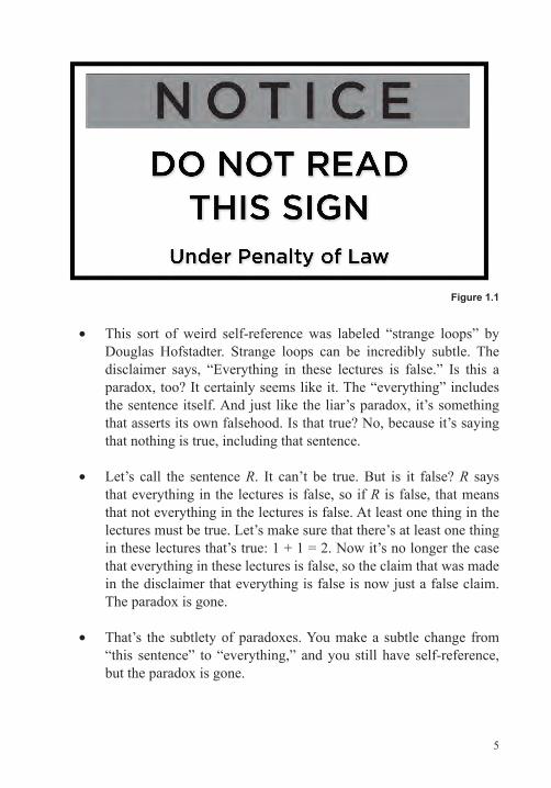
• This sort of weird self-reference was labeled “strange loops” by Douglas Hofstadter. Strange loops can be incredibly subtle. The disclaimer says, “Everything in these lectures is false.” Is this a paradox, too? It certainly seems like it. The “everything” includes the sentence itself. And just like the liar’s paradox, it’s something that asserts its own falsehood. Is that true? No, because it’s saying that nothing is true, including that sentence.

• Let’s call the sentence R. It can’t be true. But is it false? R says that everything in the lectures is false, so if R is false, that means that not everything in the lectures is false. At least one thing in the lectures must be true. Let’s make sure that there’s at least one thing in these lectures that’s true: 1 + 1 = 2. Now it’s no longer the case that everything in these lectures is false, so the claim that was made in the disclaimer that everything is false is now just a false claim. The paradox is gone.

• That’s the subtlety of paradoxes. You make a subtle change from “this sentence” to “everything,” and you still have self-reference, but the paradox is gone.

Figure 1.1

6

Lect

ure

1—Ev

eryt

hing

in T

his

Lect

ure

Is F

alse

• Let’s assume that any mathematical statement you can prove must be true and any math statement you can’t prove must be false. Then, let’s consider the sentence, “This statement is not provable.” This seems a little like the liar’s paradox.

• Can you prove it? It says that it’s not provable, so you can’t prove it. But if you can’t prove it, then it’s true. But then if it’s true, it’s supposed to be not provable, so our assumption that we could only prove the true things and the false things were all things we couldn’t prove must be wrong. This simple sentence is the basis for Kurt Gödel’s groundbreaking work in logic.

Paradoxes • Regardless of what we call mind-bending problems—paradoxes,

conundrums, enigmas, puzzles, brain teasers—there are three different ways to come to a resolution: The paradox is true (your intuition is wrong), the paradox is false (your intuition is right), or neither is the case (something deeper is going on).

• The strangest paradox in mathematics is the Banach-Tarski paradox, which roughly states that you can split a ball into a small number of pieces and reassemble them into a ball that is the same size as the original. Then, you can take the rest of the pieces and reassemble them into another ball the same size as the original. Basically, you start with 1 ball, and just by rearranging the pieces, you get 2 balls of the same size.

• For an example of how resolving a paradox can reveal something deeper and more important, we could think about Gödel’s work: “This statement is not provable.” The assumption that it’s not provable is simply false; it turns out to be incredibly complicated and very interesting.

• For an example of a paradox that ends up as false, one that tricks a surprising number of people is the travelers’ paradox. In this paradox, three weary travelers arrive at an inn. A neighbor is filling

7

in for the owner, and the neighbor says, “I think the room is $30.” So, the travelers take out their money and pay $10 each. They get settled into the room.

• The neighbor wants to make sure that he gave them the right price, so he checks with the owner. It turns out that he had the price wrong; the room was supposed to be $25, not $30. So, he decides that he will bring 5 $1 bills up to the room and pay them back. But he wonders how he is going to divide 5 $1 bills among three travelers. He decides to give one of the $1 bills to each of the travelers and then pockets the remaining $2.

• Each traveler paid $10 and got back 1, for a net of $9 each; 3 times 9 is 27, and the neighbor kept $2, so that’s 27 plus 2, which equals 29. Where did that last dollar go? This is more of a puzzle, because we know that money doesn’t disappear. It’s not really a paradox in the technical sense. The argument here has to be faulty.

• Let’s think about where the money went. We added 27, which is what the travelers paid, to 2, which is what the neighbor kept, but it makes no sense to add those two numbers. The $2 that the neighbor kept is part of the $27 that the travelers paid. They paid $27, and 2 of those dollars were in the neighbor’s pocket. The remaining $3 are in their pockets. They got $3 back, $1 each. All the money is accounted for. The $30 is split like this: $3 went back to the travelers, $2 is in the neighbor’s pocket, and $25 is with the owner.

The Barber’s Paradox • Another classic paradox is the barber’s paradox. In a certain city, all

the adult men are clean-shaven, and in this city, the barber shaves all the men who live in the city who do not shave themselves. The barber shaves nobody else. So, who shaves the barber?

• As stated so far, this is a puzzle. There are several solutions. Maybe the barber doesn’t live in the city, or maybe the barber is a woman. But what if we explicitly disallow those solutions? Let’s restate the

8

Lect

ure

1—Ev

eryt

hing

in T

his

Lect

ure

Is F

alse

question: The barber, a man who lives in a city where all the men are clean-shaven, shaves all of the men living in the city who do not shave themselves—and he shaves nobody else. Who shaves the barber? There are two cases.

○ Does he shave himself? No, he said that he shaves the men who do not shave themselves, so he can’t shave himself.

○ Does he not shave himself? If he doesn’t shave himself, and he shaves all the men who don’t shave themselves, then he’s one of the men who doesn’t shave themselves, so he must shave himself.

• Neither case works out. He can’t shave himself, and he can’t not shave himself. It’s quite a mind bender. The crux of this is that we made a simple description. We talked about a barber, and he and his customers had a certain property. And it seemed reasonable; it was a fairly simple English sentence. Our intuition says that such a property is perfectly reasonable.

• But somehow, hidden in that sentence, is a strange loop—self-reference. It turns out that that property cannot be. The barber’s paradox tells us that even a simple description might be self-contradictory. Like the liar’s paradox, it shows that a sentence might be neither true nor false.

• Bertrand Russell said that the barber’s paradox isn’t really a paradox. He said that you could make other claims about a barber, such as that the barber is both 14 years old and 83 years old. That’s a ludicrous statement; obviously, no such barber exists. Russell says that the statement of the barber’s shaving tendencies suffers from the same problem—no such barber exists.

Curry’s Paradox • Just to make sure that something in this course was true, we noted

that 1 + 1 = 2. However, now we’re going to prove that that wasn’t actually right—that 1 + 1 = 1. In order to understand this, we have

9

to remember that an if-then statement is false exactly when the hypothesis is true and the conclusion is false. The statement “If x is prime, then x is odd” is false because 2 is prime, but 2 is not odd.

• Let’s make a new sentence. We’ll call it Curry. Curry is the following sentence: “If Curry is true, then 1 + 1 = 1.” Is Curry false? The hypothesis has to be true and the conclusion false in order for it to be a false statement. For the hypothesis to be true, Curry must be true. And this is the case where Curry is false. Curry can’t be both true and false. So, Curry must be true.

• But Curry says that if Curry is true, then something else is true. And because we now know that Curry is true, then the conclusion must be true. The conclusion of Curry is that 1 + 1 = 1.

• Note that we could have put any statement in place of 1 + 1 = 1. We could have said, “Cows can fly.” We could have said, “You owe me a billion dollars.” This argument shows that every statement is true.

• What’s the resolution of this? This paradox is called Curry’s paradox, named after the American logician Haskell Curry, and it’s that we think every statement is either true or false, but our intuition is wrong.

Knights and Knaves Puzzles • Mathematician Raymond Smullyan is known for knights and

knaves puzzles, which always take place on a mythical island that is populated by knights and knaves. Knights always tell the truth; everything they say is true. Knaves always lie; everything they say is false.

• On the island of knights and knaves, suppose that you want to know whether a person is a knight or a knave, but you’re only allowed one question. The wrong question is, are you a knight? A knight would truthfully answer yes, and a knave would lie and say yes, so you can’t tell.

10

Lect

ure

1—Ev

eryt

hing

in T

his

Lect

ure

Is F

alse

• Another bad question is, are you a knave? Everybody would say no to that. It’s a version of the liar’s paradox. Nobody says, “I am a knave.” A better question is, what’s 1 plus 1? The knight would have to say 2, and the knave would say anything else, assuming that the knave didn’t know Curry’s paradox.

• Suppose that you come to a fork in the road, and one road leads to safety while the other leads to certain death. There are two guards at the fork, and you know that one is a knight and one is a knave, but you don’t know who’s who, but they do. Can you ask one of them one question and find the right path?

• One correct answer is to turn to either one of them and say, “If I ask the other guard which way leads to safety, what will he say?” When you ask that, there are two cases.

○ You ask the knight. He thinks the other guard is a knave. If you ask which road leads to safety, he will lie and point toward certain death. The knight tells the truth and therefore points toward certain death.

○ You ask the knave. He thinks the other guard is a knight. If you ask which road leads to safety, he will point you toward safety. But then the knave turns to you and lies, and he points toward certain death.

• In either case, they point toward certain death. So, your strategy is to ask the question, look which way they point, and then go in the opposite direction toward what you know is safety.

Smullyan, Satan, Cantor, and Infinity.

———, The Lady or the Tiger?

———, What Is the Name of This Book?

Suggested Reading

11

1. Why is it paradoxical for Pinocchio to say, “My nose will grow now”?

2. If some statements are neither true nor false, what happens if we create a third category and label them “unknown”?

Problems

12

Lect

ure

2—El

emen

tary

Mat

h Is

n’t E

lem

enta

ry

Elementary Math Isn’t ElementaryLecture 2

In this lecture, you will be introduced to some paradoxes and puzzles involving numbers. You might think that numbers are too simple, and it’s true that almost everything you will learn about in this lecture is based on

elementary school mathematics, but numbers are still confusing, surprising, enlightening, and surprisingly fresh. By the end of this lecture, you will discover that elementary mathematics isn’t really all that elementary. Basic numbers can hide really interesting complexity.

Berry’s Paradox • Berry’s paradox is attributed to G. G. Berry, a junior librarian at

Oxford. There are many different versions of this paradox. The following one is from Steve Walk.

• Numbers have many different descriptions in English. You could just describe the number 6 as “six,” but you could also describe it as “three times two” or “five plus one.” Sometimes the obvious description is not the shortest. You can write 999 as “nine hundred and ninety-nine,” using 28 characters, or you could write it as “one thousand minus one,” which only takes 22 characters.

• Not all numbers are describable in English with fewer than 110 characters. Why not? You can count the total possibilities. If you include uppercase, lowercase, and punctuation characters, then there are definitely fewer than 100 choices for each character. There are 110 characters, so there is a maximum of 100110, which equals 10220 possibilities. That number is larger than the number of atoms in the universe, but it’s still a finite number.

• Only finitely many numbers are describable in English with fewer than 110 characters. There is a smallest number that can’t be written with fewer than 110 characters: “the smallest natural number that

13

cannot be described in English using fewer than one hundred ten characters.” That description only used 107 characters, so our number can be written using fewer than 110 characters, and that contradicts how we found it.

• Some definitions look like they make sense, but there is some internal contradiction, which means that they don’t. There simply is no number that is the smallest describable in English using fewer than 110 characters. The description itself is self-contradictory.

• Some definitions are self-referential. And when you have self-reference, sometimes you get strange loops. And when you have strange loops, sometimes you get perplexing puzzles.

The Number 1 • The same number has different disguises. For example, the number

1 can be written as 3/3, or as 1, or as some complicated integral:

∫ tdt1 .

e

1

It’s still just the number 1. But the number 1’s most infamous disguise is 0.99999999…. The first time most people see this, they think that it must be less than 1—but it’s not.

• Everyone usually agrees that 1/3 = 0.33333333…. And if you double that, you get 2/3 = 0.66666666…. Therefore, 3/3 = 0.99999999… when you triple it. We all know that 3/3 = 1, so we’re done.

• There is another answer that isn’t a great mathematical argument but convinces many skeptics. You can always find the number that is midway between two others. It’s called the average. If 0.99999999… isn’t 1—if it’s some number that’s less than 1—what’s halfway in between the two? There’s no space to get something halfway in between the two.

14

Lect

ure

2—El

emen

tary

Mat

h Is

n’t E

lem

enta

ry

The Banach-Tarski Paradox • The Banach-Tarski paradox essentially proves that in a certain

geometric sense, 1 = 1 + 1. It says that we can take a ball, including the inside, and split it into 6 pieces. If we take 3 of those pieces and move them over and rotate them, we get a complete ball the same size as the original. We take the remaining 3 and rotate them and also get another complete ball the same size as the original.

• “Splitting” here is not meant in any physical sense. We couldn’t do this with gold, for example. But Banach-Tarski says that you can get more without adding anything, and this can be proven.

Averages • You might think that averages are simple. The average of a and b is

(a + b)/2. If you have more numbers, you just add them and divide by the number of numbers. For example, if you have 40 apples and Sara has 30 apples, then you have 35 apples on average.

• One car gets 40 miles per gallon. Another car gets 30 miles per gallon. On average, you get 35 miles per gallon—right? Actually, no: On average, you get about 34.3 miles per gallon, and that’s only if both cars drive the same distance. Averages can sometimes be tricky.

• Suppose that you’re a two-car family and both cars drive about the same amount. You have an old hybrid that gets about 50 miles per gallon, and you have a pretty old SUV that gets about 10 miles per gallon. You want to upgrade one vehicle.

• You have two options: You could upgrade the hybrid—doubling its mileage to 100 miles per gallon—or you could upgrade the SUV from 10 to 12 miles per gallon. Which upgrade saves more gas?

• Your intuition probably says that going from 50 to 100 miles per gallon saves more gas, because that’s a huge jump (100% increase). Going from 10 to 12 miles per gallon is a small jump (20% increase).

15

• Let’s do the math. Suppose that each vehicle goes 100 miles. Currently, you have a hybrid that gets 50 miles per gallon, so it uses 2 gallons of gas. The SUV gets 10 miles per gallon, so it uses 10 gallons of gas. In total, you’re using 12 gallons of gas to go 100 miles each.

• If you upgrade the hybrid, you get 100 miles per gallon. Now, the hybrid uses only 1 gallon of gas, so you saved 1 gallon of gas. But if you upgrade the SUV, you’re going 100 miles at 12 miles per gallon, which uses 8 1/3 gallons, so you save 1 2/3 gallons from the 10 gallons that you were using before. Therefore, you’re better off upgrading the SUV.

• The underlying mathematics is important, but it’s just fractions. Every fraction has two options: a/b or b/a. You want the denominator to be the reference.

• Suppose that your car gets 40 miles per gallon and Sarah’s car gets 30 miles per gallon and that you both go the same number of miles (120 miles). Let’s see why the average isn’t 35.

• You would do 120 miles at 40 miles per gallon, and it would take you 3 gallons of gas. Sarah would do 120 miles at 30 miles per gallon, so it would take 4 gallons of gas. In total, you both went 240 miles and used 7 gallons of gas: 240/7 = 34.28 miles per gallon.

• What if we did the math with miles in the denominator where they should be (as the reference value)? Find a common denominator, not a common numerator. Change all the fractions to have a common reference. Average 40 miles per gallon and 30 miles per gallon, but invert the fractions first: 2.5 gallons per 100 miles and 3 1/3 gallons per 100 miles. Add those to get 5.833333333… gallons per 100 miles. Divide by 2 to get 2.9166666666… gallons per 100 miles. If we re-invert the fraction, we get 34.28 miles per gallon. With a common reference, the denominator, it works.

16

Lect

ure

2—El

emen

tary

Mat

h Is

n’t E

lem

enta

ry

• In mathematics, this is called the harmonic mean. The arithmetic mean is the standard average. The arithmetic mean of a and b is (a + b)/2. The harmonic mean of a and b is where you add 1/a and 1/b, divide by 2, and then invert them, or take the reciprocal:

1a+ 1b

2

1

=2

1a+ 1b.

• Let’s try using harmonic mean to average speeds. Suppose that you travel at 20 miles per hour for 1 hour and then 30 miles per hour for 1 more hour. The hours are the reference, so they should be in the denominator. When you average them, you get 25 miles per hour. That’s the usual arithmetic mean.

• But if you travel 20 miles per hour for 60 miles and then 30 miles per hour for 60 more miles, what’s your average speed? This time, the reference is miles, so you have to use the harmonic average.

• Let’s plug in 30 and 20 into the harmonic average:

+=

+=

+= = × =

a b

21 1

2120

130

2360

260

2560

2 605

24.

• Let’s check just to make sure this works. If you go 20 miles per hour for 60 miles, that would take you 3 hours. If you go 30 miles per hour for 60 miles, that would take you 2 hours. In total, you’ve gone 120 miles in 5 hours: 120/5 = 24 miles per hour.

Weighted Averages • Parents of prospective college students always want to know how

much individual attention their child is going to receive. Is their student going to be fighting for the attention of a very small number of professors?

17

• Suppose that a particular college has 1700 students and 140 professors. There are three different ways you could figure out roughly how many students per professor there are.

○ First, you could count the number of students and count the number of professors and divide the number of students by the number of professors, resulting in what is usually called a head count: 1700/140 = 12 (approximately).

○ Second, you could do a survey of students. You could survey students for each one of their classes and find out how many students are in each of the professor’s classes, and then average those numbers.

○ Third, you could survey the faculty. You could ask the professors how many students are in each one of their classes, and then average their answers.

• All three of these options are some measure of how much attention a student is likely to get in an academic setting, but they result in three different numbers. The smallest number is the first method, the student-faculty ratio. The two surveys are both some measure of average class size.

• The first method is just a head count—the student-faculty ratio. That’s very different from students per class. If students took the same number of classes as professors taught, then the student-faculty ratio would be the same as the students per class. The first method (the head count) would equal the third method (the professor survey).

• Suppose that one of the classes offered by the college has about 60 students in it and that another class has only 10 students in it. When we survey the professors, both of those classes count equally: One professor submits 10 students, and the other professor submits 60. They just get submitted once.

18

Lect

ure

2—El

emen

tary

Mat

h Is

n’t E

lem

enta

ry

• But when we submit the student survey, the larger class counts 60 times. There are 60 students who submit. The smaller class counts 10 times. If it were just those two surveys, we would get 60 × 60 from the larger class and 10 × 10 from the smaller class. Adding those and dividing by 70, we get about 52.9:

×60+10× ≈60 1070

52.9.

That’s a huge difference from the professor survey, where we get (60 + 10)/2 = 35.

• Both surveys are examples of weighted averages. If we count each class once with equal weights, that’s the professor survey. If we count each class with a weight equal to the number of students in the class, that’s the student survey.

• There are many different kinds of weighted averages. In classes generally, grades are an example of a weighted average. In baseball, a batting average—hits divided by at bats—is a weighted average in which all hits are weighted equally. Wall Street has weighted averages, too; average stock prices are price weighted.

Academic grades are a common example of weighted averages.

© D

enys

Dol

niko

v/H

emer

a/Th

inks

tock

.

19

Bunch, Mathematical Fallacies and Paradoxes.

Niederman and Boyum, What the Numbers Say.

NPR, “Episode 443: Don’t Believe The Hype.”

1. A grocer buys a large number of oranges one week at a price of 3 for $1. The next week she purchases the same number, but the price has fallen to 5 for $1. Use the geometric mean formula (why?) to calculate the average price she paid for oranges over the 2-week period.

2. The following is a “proof” that 1 = 2. Find the flaw.

Take two nonzero numbers x and y and suppose that x = y. Then, we can multiply both sides by x, getting x2 = xy. Subtracting y2 from both sides gives x2 − y2 = xy − y2. Factoring both sides and cancelling the factor (x − y) gives (x + y) = y. Finally, because x = y, the left side equals 2y, yielding 2y = y, or (canceling the y’s) 2 = 1.

Suggested Reading

Problems

20

Lect

ure

3—Pr

obab

ility

Par

adox

es

Probability ParadoxesLecture 3

The puzzles and paradoxes in this lecture all involve chance. Most humans just don’t understand randomness well. If you want evidence that we’re easily tricked by probability, just look at how much money

people pour into the lotteries. In fact, the success of the entire gambling industry is our best evidence that people don’t understand probability and that mathematics education has a lot of room to improve. After this lecture, hopefully you will understand probability a little bit better.

The Three Prisoners Problem • In the three prisoners problem, proposed by Martin Gardner, there

are three prisoners: Abel, Bertrand, and Cantor. They are all on death row, but they are in separate cells. The governor is going to pardon one of them, and she puts the names in a hat and draws one randomly. Then, she sends that name to the warden, but she asks the warden not to reveal the name of the lucky man for a week.

• Abel heard that all of this had taken place, so he talked to the warden. ○ Abel: Please tell me who is going to be pardoned!

○ Warden: No, I can’t do that.

○ Abel: Okay, then tell me who is going to die.

○ Warden: That’s really the same thing.

○ Abel: Okay, but at least one of the other two will die, right?

○ Warden: Yes, I think we all know that.

○ Abel: So, you can give me that information.

○ Warden: But maybe they will both die!

21

○ Abel: Okay, here’s what you do: If Bertrand will be pardoned, tell me Cantor will die. If Cantor will be pardoned, tell me Bertrand will die. If I will be pardoned, flip a coin to name either Bertrand or Cantor as doomed.

○ Warden: Okay, but you can’t watch me flip a coin.

○ Abel: Do it tonight at home and tell me tomorrow.

○ Warden: I’ll think about it.

○ [The next day]

○ Warden: Okay, I don’t see how this will give you any more information, so I did as you suggested. Bertrand will be executed.

○ Abel: My chances of being pardoned just went up—from 1/3 to 1/2!

• Abel then surreptitiously communicated everything to Cantor, who also was happy that his chances had improved from 1/3 to 1/2! But did the two reason correctly?

• So far, this is a puzzle. Let’s turn it into a paradox. There are two different arguments. You might think that when the warden names Bertrand as doomed, he’s reducing the sample space—the space of all possible outcomes—to just two possible people being pardoned, each of them equally likely. Each has a half chance.

• Alternatively, you might think that Abel’s fate is sealed as soon as the governor chooses a name. She chooses Abel’s name 1/3 of the time, and exactly 2/3 of the time she chooses someone else. There’s nothing that the warden says or does that can change that, so Abel has just a 1/3 chance of being pardoned, and Cantor has a 2/3 chance.

22

Lect

ure

3—Pr

obab

ility

Par

adox

es

• Both of these arguments can’t be right, but they both sound valid. That’s the valid deduction from acceptable promises. This is a paradox.

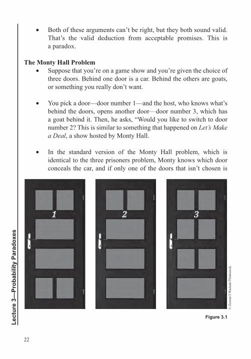
The Monty Hall Problem • Suppose that you’re on a game show and you’re given the choice of

three doors. Behind one door is a car. Behind the others are goats, or something you really don’t want.

• You pick a door—door number 1—and the host, who knows what’s behind the doors, opens another door—door number 3, which has a goat behind it. Then, he asks, “Would you like to switch to door number 2? This is similar to something that happened on Let’s Make a Deal, a show hosted by Monty Hall.

• In the standard version of the Monty Hall problem, which is identical to the three prisoners problem, Monty knows which door conceals the car, and if only one of the doors that isn’t chosen is

© Z

oona

r/J.W

acha

la/T

hink

stoc

k.

Figure 3.1

23

closed, he opens it. If he has an option of which door to open, he chooses randomly. So, should you stay with your original choice, or should you switch?

• It’s enticing but false reasoning to think that after Monty reveals the goat there are two doors left and each door is equally likely—that it doesn’t matter whether you switch or stick with your original door. That’s not correct reasoning.

• The correct reasoning is that your initial choice is correct 1/3 of the time and wrong 2/3 of the time, so if you switch, you win 2/3 of the time.

• If we enumerate all of the possibilities and count if you switch all the time, then you’re going to win 2/3 of the time. But we could also do this by analogy. Suppose that there are 1000 doors and you choose door number 816. Monty could then open every door except 816 and one other one—for example, number 142. Would you like to switch to door 142?

• Most people would say that they would switch. It’s extremely unlikely that 816 is right, and now all of a sudden door number 142 seems special. In fact, number 816 was right only 1 out of 1000 times. It’s much more likely that the prize is hiding behind the one other unopened door. If you apply this sort of thinking to three doors, you can see that switching wins, in that case, 2/3 of the time.

The Boy/Girl Problem • Like the Monty Hall and the three prisoners problems, this problem

rests very heavily on exactly how you set it up. Suppose that you have two neighbors: Art and Ed. They both moved in recently, and you met them on the driveway one day.

24

Lect

ure

3—Pr

obab

ility

Par

adox

es

• In the first conversation you have with your neighbors, you discover that both Ed and Art have two children, and each one has a girl named Sarah. Art adds that his older child is Sarah. For each of them, what’s the probability—knowing only what we know—that their other child is also a girl?

• In general, children come in two types, boys and girls, and we’ll just assume that those are equally likely (50-50). If you have two children, there are four possibilities that are all equally likely: The older and younger could be a boy and then a girl, a boy and then a boy, a girl and then a boy, or a girl and then a girl.

• We know that Art has two children and that the older one is named Sarah. That eliminates two of the possibilities. He could not have had a boy and then a girl or a boy and then a boy. Of the remaining two possibilities, one has what we’re looking for: another girl. So, of the remaining possibilities, the answer is 1/2 of the time.

• We know that Ed has two children and that one of them is named Sarah. That only eliminates the possibility that he had a boy and then a boy, leaving the other three possibilities all equally likely. Of those, only one has what we’re looking for—another girl—so the answer is 1/3 of the time. This knowledge that at least one child is a girl is simply, and very subtly, different from the knowledge that the older one is a girl, as in Art’s case.

• This is the standard mathematician’s answer, but it ignores that there’s another level of subtlety going on. This story rests on the fact that Art and Ed each have a girl with the same name. That’s much more likely to have happened to each of them if they had two girls. In fact, it’s about twice as likely. It didn’t matter that it was Art’s oldest who was named Sarah. If his youngest were named Sarah, he would have said that. So, given that they are both in this situation, the four gender pairs are no longer equally likely.

25

• For Ed, the situation is boy-girl, girl-boy, or girl-girl. The girl-girl situation is twice as likely, because there are two girls who might be named Sarah. The probabilities are 1/4, 1/4, and 1/2, respectively. How likely is it that his other child is a girl? It’s 1/2, not 1/3, as we said before.

• For Art, the situation is girl-boy or girl-girl, and now girl-girl is twice as likely. The probabilities now are 1/3 and 2/3, respectively. How likely is it that his other child is a girl? It’s 2/3, not 1/2, which is what we said before. These puzzles rely carefully on subtle assumptions.

Bertrand’s Chords • Joseph Bertrand, a 19th-century French mathematician, asked a

famous question. Take a circle, and let s be the side length of an inscribed regular triangle. If you were to take a chord—a line segment that cuts through the circle—just picking one at random, what are the chances that the chord has a length that is greater than s, the length of the triangle?

• Bertrand was able to justify three different answers to this seemingly simple problem: 1/2, 1/3, and 1/4. That’s pretty paradoxical. These solutions are in conflict; they are all different answers to the same question. What’s going on?

• The key is that we’re looking at different sample spaces. In some samples, such as a sample of basketball players, people that are more than 6 feet tall are much more prevalent than in other samples, such as a sample of children.

• In the case of Bertrand’s chords, there are different ways of sampling the chords, and in all three of these methods, we’re looking at different sample spaces. The paradox is resolved not by proving that any one of these three answers is right and the others are wrong, but by realizing that the question isn’t precise and that slightly different versions of this question lead to slightly different answers.

26

Lect

ure

3—Pr

obab

ility

Par

adox

es

Benford’s Law • In our base-10 number system that we use, every natural number

starts with a digit 1 through 9. (If we have a zero, we ignore it.) How often does each digit begin a number? If you look at the first 9 numbers, 1 is used once, 2 is used once, 3 is used once, etc. Each one of those digits is used 1/9 of the time—they’re all equal.

• If you look at the first 99 numbers, each digit is used 11 times. For example, 11 different numbers that start with a 2. Again, 1/9 of the numbers start with 2, and the same is true of all the other digits. Furthermore, of the first 999 numbers, 111 times each number will start with a 4. And the same is true of all the other digits. It seems like each one of the digits starts 1/9 of the numbers that exist.

• But in 1881, astronomer Simon Newcomb thought it might be possible that more numbers were starting with 1 than with other digits. It turns out that it’s strange, but true—for many, many different sources of numbers.

• This is later named Benford’s law, after Frank Benford, who found that the numbers from many different sources—city populations, molecular weights, addresses—obeyed the same distribution. Almost 30% of the numbers he analyzed started with 1, about 18% of numbers started with 2, about 13% started with 3—decreasing to 9, with only about 5% of these numbers starting with 9

• Like many other problems, the sample space matters here. If you’re using numbers from 1 to 999, the digits are equally likely. But if you’re using data from a real source, then it obeys Benford’s law.

Gorroochurn, Classic Problems of Probability.

Rosenhouse, The Monty Hall Problem.

Suggested Reading

27

1. Let’s revisit the Tuesday birthday problem. You meet a woman and learn that she has two children and that one of them is a son who was born on a Tuesday. What’s the probability that the other one is also a son?

2. The following is a bridge conundrum from Martin Gardner’s Mathematical Puzzles & Diversions: Suppose that you are dealt a bridge hand (13 random cards out of a standard 52-card deck). Following are two probabilities that you might calculate while looking through your cards:a. If you see an ace, what’s the probability that you have a second ace?

b. If you see the ace of spades, what’s the probability you have a second ace?

One of these is greater than 50%; the other is less than 50%. Which is which?

Problems

28

Lect

ure

4—St

rang

enes

s in

Sta

tistic

s

Strangeness in StatisticsLecture 4

In this lecture, you will be exposed to statistical paradoxes and puzzles. People sometimes use statistics to mislead other people. When dealing with statistics, there are ways to doctor graphs, and sampling problems

can be present. In addition, it is important to keep in mind that correlation is not the same as causation. Studying statistical paradoxes can improve our thinking, and it can correct our naïve conceptions of the world and how the world works.

Batting Averages • There are different kinds of averages. The mean of a group of

numbers is found by adding and then dividing by the number. The median is the middle number, with half of the data on each side. The mode is the most frequent number. The differences among these can be really large, depending on how the numbers are distributed.

• Stephen Jay Gould, a paleontologist and an evolutionary biologist, used ideas of distribution to give a very mathematical answer to a sports question: Why is it that nobody in baseball has hit .400—meaning that a batter gets a hit 4 out of every 10 times—since Ted Williams did it in 1941?

• Generally, athletic performance has gotten better over time. But maybe the reason that nobody can get back to .400 is that it’s not measured against some sort of arbitrary standard. Instead, it’s pitching versus hitting. And maybe both pitching and hitting got better, but pitching got better faster.

• But that’s not the case. Across the league, the mean batting average has stayed roughly stable, at about .260. So, the puzzle remains.

29

• Standard deviation is a measure of how far a set of data is spread away from its median—away from the average. If something has a large standard deviation, the data is really spread out. If it has a small standard deviation, the data is heavily concentrated.

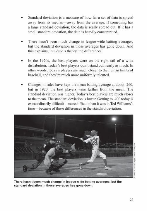
• There hasn’t been much change in league-wide batting averages, but the standard deviation in those averages has gone down. And this explains, in Gould’s theory, the differences.

• In the 1920s, the best players were on the right tail of a wide distribution. Today’s best players don’t stand out nearly as much. In other words, today’s players are much closer to the human limits of baseball, and they’re much more uniformly talented.

• Changes in rules have kept the mean batting average at about .260, but in 1920, the best players were farther from the mean. The standard deviation was higher. Today’s best players are much closer to the mean. The standard deviation is lower. Getting to .400 today is extraordinarily difficult—more difficult than it was in Ted Williams’s time—because of these differences in the standard deviation.

There hasn’t been much change in league-wide batting averages, but the standard deviation in those averages has gone down.

© D

onal

d M

iralle

/Dig

ital V

isio

n/Th

inks

tock

.

30

Lect

ure

4—St

rang

enes

s in

Sta

tistic

s

Medical Statistics • Suppose that you have some serious condition—for example,

hypertension—and to avoid having a stroke, you need medication. You might have three choices. Medication A reduces stroke chances by 4 percentage points. Medication B decreases your chances of having a stroke by 40%. When given to 25 patients, the chances are that medication C will prevent one stroke. Which one would you choose?

• If you’re like most people, you choose option B, which offers a 40% reduction. The surprise is that all three might describe the same medication.

• Suppose that you had a control group and that 10% of them had a stroke, and then there was the treatment group, who received the medication, and 6% of them had a stroke. Your absolute risk reduction—where you take the percentage minus the other percentage, or 10% minus 6%—is 4%. In other words, your risk goes down by 4 percentage points.

• Your relative risk reduction went down from 10 percentage points to 6 percentage points, and you divide by the original, the 10%: 4%/10% = 40%. In other words, the 4-percentage-point decrease was 40% of the original 10% risk. Your risk goes down by 40%.

• The third statistic was the number needed to treat. To get the number needed to treat, you look at the absolute risk reduction and take 1 over that number. In this case, the absolute risk reduction was 4%: 1/(4%) = 25. In other words, if 25 patients were treated with this drug, one stroke would be prevented.

• How misleading is this? In a study of medical students who are presented with the fictitious choice of whether or not to give chemotherapy, if they learned just the relative risk—in this case, the 40% decrease—70% of the medical students chose to give the chemo. If they learned other equivalent statistics, including the three above, with all of that information, only 45% of medical

31

students chose to give the chemo. The same drug, same statistics, and same underlying numbers, just presented in different ways, gave them different impressions, and they made different decisions.

Courtroom Statistics • Suppose that you’re sitting on a jury, and you’re analyzing a

particular crime. The prosecution says, “We pulled a partial fingerprint, and it matches the defendant. The science of fingerprints says that this particular fingerprint would likely only match 1 out of 100,000 people.”

• Given only this information, how certain are you that the defendant was involved? What are the chances that the defendant was innocent, and what other questions would you want answered?

• Given the fingerprint statistic (1 out of 100,000), there are 99,999 out of 100,000 chances that this person is involved and only 1 out of 100,000 chances that the person is not involved. If no more information is given, most people might succumb to what’s called the prosecutor’s fallacy.

• Suppose that there was a ton of other evidence that pointed to a particular person, and only then did they arrest that particular person and then check the fingerprints. The fingerprint matches. That’s actually really good evidence. The odds of that particular person matching were indeed very small. But there’s another possibility, and somebody in the jury might not know which of these possibilities it is. It’s fallacious reasoning.

• Suppose that they found a fingerprint at the scene, and then they tested it against a really large database and found one hit. Then, they arrested that person, the defendant. And that’s all the evidence they have.

• That’s really misleading. You need important pieces of information in order to understand the statistics here. You need the size of the local population as well as the size of the database. If the local

32

Lect

ure

4—St

rang

enes

s in

Sta

tistic

s

population has a million people, then a million divided by 100,000 means that 10 people should be a match. Where are the other 9? They are equally likely as the defendant to be guilty; it just happens that they weren’t in the database.

• And how big is the database? Suppose that there are 200,000 people in this database. What are the chances that this crime scene fingerprint doesn’t match any of them? The chances that it doesn’t match any one of them are 999,999 out of 100,000. Therefore, the chance of all 200,000 of these people not matching is 999,999/100,000200,000, or 13.5%.

• This means that there is an 86.5% chance of at least one of them matching. That’s random—there’s no reason for that guilt. It’s just by chance. This is called data dredging: Sift through enough data and you’ll find something that matches just by chance.

• Mathematically, the problem is that we’re mixing up two different probabilities. We have two different sample spaces. The 1 out of 100,000 is the chance of a match if we know someone is innocent. What we want is the chance of the person being innocent if we know someone is a match. In mathematical terms, what we know is the probability of A given B—written P(A|B)—but we want the probability of B given A, or P(B|A). Those are different, but they’re related by what’s called Bayes’s theorem.

• If you know the chance of a match if we know someone’s innocent is 1 out of 100,000, the sample space is all innocent people. What we want is the chance of being innocent if we know someone’s a match. The sample space is all of the people who match the fingerprint. If the population is large enough, the sample space is actually quite large.

Simpson’s Paradox • Suppose that LeBron James and Kevin Durant are playing

basketball. In the first half, Durant outshoots LeBron—he shoots a better percentage. In the second half, Durant again shoots a better

33

percentage than LeBron. For the whole game, Durant must’ve shot a better percentage than LeBron—right? No. That might not be the case. It might be an example of Simpson’s paradox, named after Edward Simpson.

• How is it possible that Durant might outshoot LeBron in both halves but not over the whole game? Durant might have gone 1 for 7 in the first half and 3 for 3 in the second. LeBron might have shot 0 for 3 (horrible) in the first half and 5 for 7 (pretty good) in the second.

• In both halves, Durant outshoots LeBron. In the first half, Durant outshoots LeBron because LeBron shot 0%; in the second half, Durant outshoots LeBron because Durant shot 100%. But if you look at the whole game, Durant shoots 4 for 10 overall. LeBron shoots 5 for 10. LeBron outshoots Durant 50% to 40% over the whole game.

• Let’s analyze this with variables. If Durant outshoots LeBron in two halves, we feel like it should mean that Durant outshot LeBron for the full game. If Durant shoots a/b in the first half and then c/d in the second half, and LeBron shoots w/x and then y/z, our intuition says that if we add Durant’s numbers, we should get more than if we add LeBron’s numbers, because Durant outshot LeBron in both halves.

• It’s true that the sum of a/b + c/d is bigger than the sum of w/x + y/z, but it’s not the sum that we’re interested in. When you add fractions, a/b + c/d, you have to find a common denominator, bd, and you end up with (ad + cb)/bd.

• What we want isn’t that sum. We want the made shots over the total attempts. We want the sum of the numerators over the sum of the denominators, and those two are different. Our intuition is correct, but only for the sum. The sum of Durant’s fractions is indeed larger than the sum of LeBron’s. We aren’t adding fractions. We’re adding ratios, so we need to add both the numerator and the denominator. The same thinking doesn’t apply to the sum of ratios.

34

Lect

ure

4—St

rang

enes

s in

Sta

tistic

s

• It turns out Simpson’s paradox isn’t just about splitting things into two pieces. You could compare numbers over four quarters, or even more. Durant can beat LeBron in each one of those subdivisions and still lose overall. A relationship over all the subgroups doesn’t guarantee the same relationship over the entire thing.

Gould, Full House.

Huff, How to Lie with Statistics.

Mlodinow, The Drunkard’s Walk.

Pearl, Causality.

1. Suppose that a drug reduced the chances of having a heart attack among patients of your age, sex, and general health from 1% to 0.5%. Describe the effectiveness of this drug in three ways: absolute risk reduction, relative risk reduction, and number needed to treat.

2. If you were sitting on a jury and the prosecution claimed that some piece of physical evidence tied the accused to the crime with a certainty of 1 in 100 million, what questions should you ask about the investigation?

Suggested Reading

Problems

35

Zeno’s Paradoxes of MotionLecture 5

Zeno of Elea, who lived in the 5th century B.C.E., was a student in the Eleatic school of Parmenides, an early Greek philosopher who believed that all reality is one—immutable and unchanging.

According to Plato, Zeno’s paradoxes were a series of arguments meant to refute those who attacked Parmenides’s views. Of the five surviving paradoxes of Zeno of Elea, only the last one is taken from a text that actually purports to quote Zeno. All the others are passed down through many hands. The four paradoxes are about motion in one form or another. The fifth paradox is about plurality (how a continuum might be divided up into multiple parts).

Zeno’s Paradoxes • The following two paradoxes are the two most famous of Zeno’s

five paradoxes. Let’s call the first paradox Achilles and the tortoise. Imagine Achilles, who was the fastest of the Greek warriors, racing against a very slow tortoise. That’s not a fair race, so let’s give the tortoise a slight head start.

• Zeno says that it’s not possible for Achilles to win. It will take some small amount of time for Achilles to get to where the tortoise started, and in that time, the tortoise will have moved forward. Then, it will take Achilles some time to get to that point, and in the meantime, the tortoise will have moved forward.

• And this process continues. Achilles never passes the tortoise, always just making up ground to where the tortoise just left. It’s an infinite number of catchings that Achilles has to do. It’s not possible.

• The second paradox, sometimes called the dichotomy, is more fundamentally about motion—it’s the dichotomy that you can’t start or finish a trip. It’s only one person or object now. The first

36

Lect

ure

5—Ze

no’s

Par

adox

es o

f Mot

ion

version of this paradox is that motion is impossible. In order to get anywhere, first you have to go halfway. Then, you’d have to go half of the remaining distance, and then half the remaining distance, and then half, and then half, and then half. To arrive, you’d have to complete an infinite number of steps.

• The second version is even worse than the first. Not only can’t you get anywhere, but you can’t even start anywhere. Zeno says that in order to get somewhere, you’d have to first get to the halfway point. And before that, you’d have to go halfway to the halfway point. And before that, you’d have to go halfway to the halfway to the halfway point—and so on. Because there are an infinite number of steps before you get anywhere, Zeno says that you can’t start.

• The third paradox is usually called the arrow. This is Zeno again arguing that motion is impossible. To paraphrase it, the arrow in flight is at rest. For if everything is at rest when it occupies a space equal to itself, and what is in flight at any given moment always occupies a space equal to itself, it cannot move.

• In other words, the arrow can’t move during an instant. When we would break down that instant into smaller parts, instant, by definition, is the minimal—the indivisible time unit. And at any instant, the arrow occupies only its own space. So, at no time is it moving. It’s always motionless.

• The fourth paradox is sometimes called the stadium. Consider three rows of people seated in a stadium. The people in the top row—we’ll call them the A’s—never move. But the people in the middle row, the B’s, move to the left at one seat per time step. And the bottom row, the C’s, move to the right at one seat per time step. In any one time step, each B passes exactly one A. And the same is true of the C’s: Each time step, the C’s pass exactly one A.

37

• But think about the B’s passing the C’s. At every time step, each B passes two C’s. They’re moving in opposite directions. At first, it seems like there’s really nothing here—that Zeno is just missing the idea of relative motion. The B’s are moving relative to A at one speed. The B’s are moving relative to the C’s at twice that speed, so they pass twice as many C’s per time.

• Here’s the paradoxical part. Let’s assume that time is quantized—that it’s discrete—into individual instants and that the rows move one seat per instant. Now look at the motion. As we move from one instant to the next, each B passes one A. And the same goes for the C’s passing the A’s, one per instant. But when do the B’s pass the C’s? Somehow, that happens twice per instant, and we have to break time down further. But the instant was the smallest piece of time. That’s where we started this argument.

• And that’s Zeno’s real point. The key distinction is between continuous, like a number line (a range of values, or a continuum, that you can change as much or as little as you want), versus discrete, like a string of pearls (one then the next—only certain amounts are allowed, and in between those, not allowed).

• Are space and time continuous? Achilles and the tortoise, as well as the dichotomy, argue that they are not. You can’t break down each half into smaller halves. Are space and time discrete? The arrow and stadium arguments argue that they are not. You have to be able to find smaller divisions.

• Parmenides’s view is that reality is unchanging and immutable. Zeno’s paradoxes are designed to support this view. Is reality continuous? That’s refuted by the first and second paradoxes about motion. Is reality discrete? That’s refuted by the third and fourth paradoxes about time. The conclusion is that reality is an illusion. Zeno is making a serious metaphysical argument that’s hotly debated among philosophers.

38

Lect

ure

5—Ze

no’s

Par

adox

es o

f Mot

ion

The Mathematical Approach to Zeno’s Paradoxes • How does mathematics answer Zeno’s paradoxes? The key

mathematical idea in Zeno’s paradoxes was finally resolved by accepting the following fact: When you add an infinite number of positive numbers, sometimes the result is finite—not infinity.

• This is a bit counterintuitive. Think about a number line. When you add a positive number, you move to the right. Then, you add another positive number and go farther right. Then, you add another one and keep going to the right. If you do that an infinite number of times, it seems like you should march off to infinity. But you might not actually go to infinity.

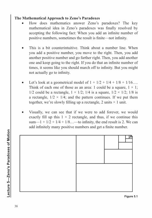
• Let’s look at a geometrical model of 1 + 1/2 + 1/4 + 1/8 + 1/16…. Think of each one of those as an area: 1 could be a square, 1 × 1; 1/2 could be a rectangle, 1 × 1/2; 1/4 is a square, 1/2 × 1/2; 1/8 is a rectangle, 1/2 × 1/4; and the pattern continues. If we put them together, we’re slowly filling up a rectangle, 2 units × 1 unit.

• Visually, we can see that if we were to add forever, we would exactly fill up this 1 × 2 rectangle, and thus, if we continue this sum—1 + 1/2 + 1/4 + 1/8…—to infinity, the end result is 2. We can add infinitely many positive numbers and get a finite number.

Figure 5.1

39

• We never get past 2, but we get as close to 2 as we wish. This is the key calculus idea of a limit. This series is just one of a very general type of series called geometric series. The key property is that to get from one term to the next, you have to multiply by some fixed number. In the case of this series, we’re multiplying by 1/2 each time, to go from 1 to 1/2 to 1/4 to 1/8.

• Zeno’s first two paradoxes—Achilles and the tortoise and the dichotomy—are really just geometric series in disguise. With Achilles and the tortoise, we can’t get anywhere. First, we have to go halfway there, and then half the remaining distance, and then half the remaining distance. Zeno said that there are infinitely many trips—you’re never done. Calculus says that infinitely many trips can add up to a finite distance, and the time those trips take can take just a finite time.

• A similar explanation can be made for Achilles and the tortoise. The calculus view is that you can finish an infinite process, so Achilles does, in fact, catch up with tortoise, and then passes it. Aristotle poses this difference between actual infinity and potential infinity. Actual infinity is the end result of infinitely many steps. In some sense, that is what a limit is. Potential infinity is only the process of doing something again and again. You never actually get to the end.

• We can add infinitely many positive numbers and get a finite number, but do we always get a finite number? If we were adding 1 + 1 + 1 + 1 + 1…, we would clearly go off toward infinity. But what if the numbers got smaller and smaller, closer to 0—for example, 1 + 1/2 + 1/3 + 1/4 + 1/5 + 1/6…. If you keep adding, do you get to a finite number, or do you get infinity?

• That’s not an easy question, but it is one that’s covered in calculus. That series is called the harmonic series, and it has to do with string harmonics. The answer is that you actually get infinity. To show that you get infinity, you can find a smaller series that definitely goes to infinity, and then the larger series, the harmonic series, which is bigger than it, must also go to infinity.

40

Lect

ure

5—Ze

no’s

Par

adox

es o

f Mot

ion

• Both of Zeno’s last two paradoxes—the arrow paradox and the stadium paradox—deal with the discreteness of time. What’s the resolution of the arrow paradox? Does the arrow never move? There are two ways out of this: Zeno’s arguments might be inherently flawed, or maybe time just isn’t discrete.

• Zeno describes the arrow as “at rest” at each moment and, thus, not “in motion” at any instant. But the idea “in motion” requires a range of instants. Motion means that you’re in different places at different instants. In fact, even the idea of being at rest requires a range of instants. When you’re at rest, you have to be in the same place at different times, at different instants. If you’re thinking about things at a single instant—the arrow captured in a picture—it’s not really in motion or at rest. Neither “in motion” nor “at rest” apply to a single instant.

• A second way out of Zeno’s trap is that time just isn’t discrete—that any interval of time consists of infinitely many instants. The number line, after all, is a continuum. It’s not separated points. It’s not a string of pearls.

• This is sometimes described as an “at-at” theory of motion. At one time, the arrow is at one position. At a different time, it’s at a different position. We avoid trying to create intervals of time out of these individual instants. After all, if no time passes during any one instant, then no time passes during any collection of those instants. This is foreshadowing the problems that might happen with infinity.

• Granting that time isn’t discrete means that you have to deal with infinity. Every interval of space, and maybe every interval of time, is made up of infinitely many moments and even infinitely many smaller intervals of time. Dealing with infinity gets more complicated than you might think. It’s full of many interesting paradoxes.

41

Al-Khalili, Paradox.

Salmon, ed., Zeno’s Paradoxes.

1. One way of describing the fact that the harmonic series (1 + 1/2 + 1/3 + 1/4 + 1/5 + 1/6 +…) diverges (i.e., gets as large as you’d like), but does so very slowly, is the following: If you ask someone to give you the largest number he or she can name and add up that many terms of the series, the sum will be less than 300—but if you add up infinitely many terms, you get infinity. Explain the apparent contradiction.

2. In Zeno’s dichotomy paradox, he argues that you can never even start a trip. The reasoning is as follows: Any trip must at some point arrive at the halfway point. Prior to that, it must arrive at the point halfway to the halfway point. Continuing the argument, there are an infinite number of steps to take (each to get to a nearer halfway point), and there is no first step. Hence, the trip can never be started. What’s the modern mathematician’s response?

Suggested Reading

Problems

42

Lect

ure

6—In

finity

Is N

ot a

Num

ber

Infinity Is Not a NumberLecture 6

Imagine that you own a hotel. Your hotel has infinitely many rooms: room 1, room 2, room 3, room 4, stretching down an infinite hallway. This is Hotel Infinity. Sometimes people call this Hilbert’s Hotel, for

German mathematician David Hilbert. In this lecture, you will learn about the beginning of infinity, in all of its strange, paradoxical glory. As you will learn, infinity introduces some really serious mathematical questions. In addition, you will learn about completing supertasks, which are very theoretical and philosophical.

Hotel Infinity • At Hotel Infinity, business is good. All of the rooms are full. So,

do you hang the “No Vacancy” sign in front of the hotel? What if someone comes and desperately wants a room?

• There’s actually no problem. You get on the hotel’s public address (PA) system and say, “Everyone, please pack up your things and move down one room.” The person in room 1 moves to 2, the person in 2 moves to 3, the person in 3 moves to 4, and so on. In general, the person in room n moves to room n + 1. Your new guest just goes into room 1. It’s empty.

• This is very different from finite hotels. In this case, you could add somebody to a hotel that was already full.

• What if your new visitor was extremely picky and demanded a particular room, such as room 496? Can you accommodate somebody like that? Sure, there’s still no problem. You get on the PA system and say, “If your room is number 496 or above, please move down one room.” Room 496 becomes vacant, and the picky visitor is happy.

43

• What if it’s not just one visitor? What if 10 new guests arrive? You can do that, too: “If your room number is n, please move to n + 10.” The person in room 1 moves to 11, 2 moves to 12, and so on. Then, the first 10 rooms are free. In fact, this strategy works for any finite number of guests.

• This is really strange. If you have finitely many rooms and they’re all filled, you can’t accommodate anyone. Some sizes of infinity seem different, but they aren’t. The key is about matching—a 1-to-1 correspondence.

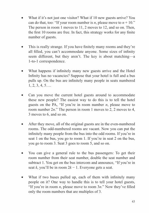
• What happens if infinitely many new guests arrive and the Hotel Infinity has no vacancies? Suppose that your hotel is full and a bus pulls up. On the bus are infinitely many people in seats numbered 1, 2, 3, 4, 5….

• Can you move the current hotel guests around to accommodate these new people? The easiest way to do this is to tell the hotel guests on the PA, “If you’re in room number n, please move to room number 2n.” The person in room 1 moves to 2, 2 moves to 4, 3 moves to 6, and so on.

• After they move, all of the original guests are in the even-numbered rooms. The odd-numbered rooms are vacant. Now you can put the infinitely many people from the bus into the odd rooms. If you’re in seat 1 on the bus, you go to room 1. If you’re in seat 2 on the bus, you go to room 3. Seat 3 goes to room 5, and so on.

• You can give a general rule to the bus passengers: To get their room number from their seat number, double the seat number and subtract 1. You get on the bus intercom and announce, “If you’re in seat k, you’ll be in room 2k − 1. Everyone gets a seat.

• What if two buses pulled up, each of them with infinitely many people on it? One way to handle this is to tell your hotel guests, “If you’re in room n, please move to room 3n.” Now they’ve filled only the room numbers that are multiples of 3.

44

Lect

ure

6—In

finity

Is N

ot a

Num

ber

• You go to the first bus—bus A—and say, “If you’re in seat k, you’re going to go to room 3k − 2.” The person in seat 1 goes to room 1, seat 2 goes to room 4, seat 3 goes to room 7, and so on. You go up by 3 each time. Notice that if you divide any of those numbers by 3, you get a remainder of 1.

• Then, you go to the second bus—bus B—and say, “If you’re in seat j, you’re going to be in room 3j − 1.” The person in seat 1 goes to room 2, seat 2 goes to room 5, seat 3 goes to room 8, and so on. You go up by 3 each time again. And, again, notice that if you divide any of the room numbers by 3, you get a remainder of 2.

Infinite Buses and People • What if you had infinitely many buses, each with infinitely many

people, pull up? Can you still find a room for everyone?

• The notation here gets a little confusing. We have numbers on the hotel rooms, and now we have letters on the buses. We’ll call them A, B, C, …, but we have to pretend that the alphabet goes on forever. And on each bus we have seats, so maybe on bus A we call those seats A1, A2, A3, A4, ….

• Amazingly, it’s still possible to get everybody from the buses into the hotel rooms. There are two different arguments for this.

• The first argument involves zigzagging through the buses, starting by lining up the new guests in a very particular way. We take the first person from bus A and then the second person from bus A, followed by the first person from bus B. Then, we take the third person from A, the second person from B, and the first person from C. The next four people in line would be the fourth person from A and then B3, C2, and D1. (See Figure 6.1.)

• It’s easier to see the pattern if we line up the buses in a particular way. Pull up the first bus all the way. Pull the second one up a little short. Stop the next bus even sooner—and so on. Line up each bus so that the first seat lines up with the second seat on the

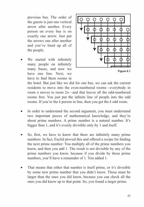
45

previous bus. The order of the guests is just one vertical arrow after another. Every person on every bus is on exactly one arrow. Just put the arrows one after another and you’ve lined up all of the people.

• We started with infinitely many people on infinitely many buses, and now we have one line. Next, we have to find them rooms in the hotel. But just like we did for one bus, we can ask the current residents to move into the even-numbered rooms—everybody in room n moves to room 2n—and that leaves all the odd-numbered rooms free. You just put the infinite line of people into the odd rooms. If you’re the k person in line, then you get the k odd room.

• In order to understand the second argument, you must understand two important pieces of mathematical knowledge, and they’re about prime numbers. A prime number is a natural number. It’s bigger than 1, and it’s evenly divisible only by 1 and itself.

• So, first, we have to know that there are infinitely many prime numbers. In fact, Euclid proved this and offered a recipe for finding the next prime number: You multiply all of the prime numbers you know, and then you add 1. The result is not divisible by any of the prime numbers you know, because if you divide by those prime numbers, you’ll have a remainder of 1. You added 1.

• That means that either that number is itself prime, or it’s divisible by some new prime number that you didn’t know. Those must be larger than the ones you did know, because you can check all the ones you did know up to that point. So, you found a larger prime.

Figure 6.1

46

Lect

ure

6—In

finity

Is N

ot a

Num

ber

• The second thing we have to know is unique prime factorization. Every number can be uniquely written as the product of prime numbers. For example, 28 = 22 × 7, and there’s no other way to do it.

• How do we use these two facts to solve our problem of putting infinitely many people on infinitely many buses into our hotel? Like before, we move the current guests into the even-numbered rooms, and now we go back to the buses and label the buses with prime numbers, starting at 3.

• The first bus is labeled 3. The next bus is labeled 5, and the next is 7. We skip 9, because 9 isn’t prime—nor are 11, 13, or 15. We start again with 17, 19, 23, 29…. As an example, if you’re on bus number 5 in seat number 3, you’re going to go to room 53, which is 125. If you’re on bus number 13 in seat number 6, you’re going to go to room 136, which is 4,826,809. In general, if you’re on bus k in seat j, you’re going to go to room k j.

• There are infinitely many people on infinitely many buses, and they are all accommodated with rooms in Infinity Hotel, but there are still some rooms unoccupied if we do it this way. All the even-numbered rooms are full, with the old guests. But what about room 15? 15 = 3 × 5. It’s not just a power of a single prime, so nobody’s in that room. Any product of odd primes does the same thing. For example, room 63 is empty. 63 = 9 × 7.

• In fact, there are still infinitely many rooms available. The key idea is to use the powers of primes to fit in more stuff. It turns out that this idea was key to Gödel’s proof.

Supertasks • The idea of supertasks is completing infinitely many tasks in a finite

amount of time. It leads to many different paradoxes. It’s closely related to Zeno’s paradoxes. Think about the dichotomy, which involved going halfway to the goal each time.

47

• The philosopher James Thompson thought about a 1-minute game where you turn a lamp on or off at each time step. You do it once in the first 30 seconds, and then 15 seconds, and then 7.5 seconds. As you get halfway toward 1 minute, you do it again and again. At the end of the game, is the lamp on or off? Or maybe it’s both.

• In 2001, British mathematician E. Brian Davies used this idea to theorize the existence of an infinitely powerful computer. Imagine that you could create a machine that could replicate itself, but instead of replicating exactly itself, it replicated a faster version of itself—a machine that’s twice as fast, for example. And the next generation replicates itself as a machine that is, again, twice as fast.

• Suppose that the machines could do simple arithmetic and communicate with each other. What you end up with is arbitrarily fast computers. Of course, Davies admits that the physics of quantum mechanics and thermodynamics means that this isn’t actually possible, but it is interesting to think about.

• How far away from this are we? As an example, 3-D printing technology allows us to make objects, but how long will it be before a machine can self-replicate completely? And how long will it be before it could make a version of itself that’s even faster than that? What would that mean?

• Supertasks like these are all a bit self-referential, and they’re at the heart of many paradoxes and conundrums, many of them involving infinity. For example, we discussed 1 being equal to 0.99999999…. Many people think of 0.99999999… as a supertask. You keep writing down 9s. You never finish, or at least you don’t finish in any finite time. To understand that it actually does equal 1, the supertask has to somehow have an end. You have to do infinitely many tasks in a finite amount of time.

48

Lect

ure

6—In

finity

Is N

ot a

Num

ber

Dauben, Georg Cantor.

Dunham, Journey through Genius.

Smullyan, Satan, Cantor, and Infinity.

1. How are Zeno’s paradoxes (and the fact that motion is, in the end, possible) similar to the supertask described in the Ross-Littlewood paradox? How are they different?

2. The Ross-Littlewood paradox makes it seem like any combination of balls might be in the vase at the end of the exercise in the video. That’s not quite the case. Why not?

Suggested Reading

Problems

49

More Than One InfinityLecture 7

Most people think that infinity is just one thing, but it turns out that there are different sizes of infinity. In this lecture, you will be introduced to the groundbreaking work of German mathematician

Georg Cantor, who tamed infinity. At one time very controversial, Cantor’s work is now accepted by all mathematicians. Understanding Cantor’s work gives you a greater appreciation for sets of numbers and how complicated the seemingly simple number line is. It gives you a better understanding of the numerical world.

1-to-1 Correspondence • Georg Cantor tamed infinity. He figured out how we should study

it. His fundamental insight was about the size of infinite sets. The problem is that if you have finite sets, you can count them. But if you have infinite sets, what does size mean?

• Cantor’s solution is the idea of a 1-to-1 correspondence. With finite sets, you have two options if you want to think about the size: You could count a finite set or match it with a set whose size you already know. For infinite sets, counting fails. You would count forever. But matching still works.

• If two sets have the same size, they have the same cardinality. And two sets have the same size if it is possible to find a 1-to-1 correspondence between them. But we have to be careful: We’re not saying that every matching is a 1-to-1 correspondence. We’re saying that there is a 1-to-1 correspondence.

• A 1-to-1 correspondence seems like a very simple idea: There are two sets, and they’re the same size. They’re the same cardinality if you can match them up. It works for finite sets, and it works

50

Lect

ure

7—M

ore

Than

One

Infin

ity

for infinite sets. Once Cantor had this initial idea, he started to explore the implications of it. To explore the implications, let’s explore infinite sets and ask whether they are the same size or different.

Natural Numbers • Are the natural numbers at the same cardinality as the even positive

natural numbers—2, 4, 6, 8…? When you map the even numbers to the natural numbers, there’s an obvious mapping. You can just match 2 to 2, 4 to 4, 6 to 6…. But that’s not a 1-to-1 correspondence. Some numbers are missed—the odd numbers.

• Is there another one that would work? It’s not too difficult to figure this out. Both lists are already in order, so we just put them in that order. We match 2 to 1, 4 to 2, 6 to 3, …. In general, 2n matches to n. The positive even numbers, therefore, have the same cardinality as the natural numbers. It’s the same size. We can match them up in a 1-to-1 manner.

• We call this countable. Any set that has a 1-to-1 correspondence, or matching, within the set of natural numbers is countable. If we can count them—matching something up with 1, something with 2, something with 3, and so on—then it’s a countable set.

• The even numbers are a subset of the natural numbers. In fact, it’s a proper subset, which means that some numbers are not in the subset. Do we match the full set with half of it, the natural numbers with the even numbers? Finite sets don’t work this way.

• With infinite sets, you can match up a proper subset with the entire set. In this case, we’re matching the even numbers up with the natural numbers. Every natural number is matched with an even number; every even number is matched with a natural number. Nothing is missed, and there’s no doubling up.

51

• The even numbers are, in some sense, half of the natural numbers. But they get matched up with all of the natural numbers. It’s paradoxical—counterintuitive—because it works differently for infinite sets than finite ones.

Integers • Integers include not just 1, 2, 3, 4,…, but also 0, −1, −2,…. Can you

match those up with the natural numbers? Again, the natural way doesn’t work. You could match 1 with 1, 2 with 2, 3 with 3, …, but you’re missing all the negative numbers and 0.

• One way to do it is to match 1 with 0, and then 2 with 1, and then 3 with −1, 4 with 2, 5 with −2…. In general, you could take the even numbers, 2n, and map it to n, and that would result in all the positive numbers. Then, you could take the odd numbers, 2n + 1, and map it to −n.

• You can check that nothing is missed and nothing is doubled up. This is, indeed, a 1-to-1 correspondence.

Rational Numbers • Rational numbers are all the possible fractions, such as 1/4,

3/16, and −41/13. There are infinitely many fractions, or rational numbers, between 0 and 1. There are infinitely many between 1 and 2. You can’t possibly match all of those up with just one copy of the natural numbers, can you? Yes, you can. In fact, there are two arguments: The first argument uses infinite buses, and the second argument uses prime factorization.

• First, let’s show that the positive rational numbers are countable, using a bus argument. Bus 1 has all the fractions with 1 in the denominator in order: 1/1, 2/1, 3/1, 4/1…. Bus 2 has all the fractions with 2 in the denominator that aren’t already on bus 1: 1/2, 3/2, 5/2, 7/2…. On bus 3 is all the fractions with a 3 in the denominator that aren’t already on buses 1 or 2: 1/3, 2/3, 4/3, 5/3…. Every positive rational number is on exactly one of these buses.

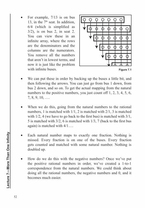
52

Lect

ure

7—M

ore

Than

One

Infin

ity

• For example, 7/13 is on bus 13, in the 7th seat. In addition, 6/4 (which is simplified as 3/2), is on bus 2, in seat 2. You can view these in an infinite array, where the rows are the denominators and the columns are the numerators. You remove all the numbers that aren’t in lowest terms, and now it is just like the problem with infinite buses.

• We can put these in order by backing up the buses a little bit, and then following the arrows. You can just go from bus 1 down, from bus 2 down, and so on. To get the actual mapping from the natural numbers to the positive numbers, you just count off 1, 2, 3, 4, 5, 6, 7, 8, 9, 10, ….

• When we do this, going from the natural numbers to the rational numbers, 1 is matched with 1/1, 2 is matched with 2/1, 3 is matched with 1/2, 4 (we have to go back to the first bus) is matched with 3/1, 5 is matched with 3/2, 6 is matched with 1/3, 7 (back to the first bus again) is matched with 4/1….

• Each natural number maps to exactly one fraction. Nothing is missed. Every fraction is on one of the buses. Every fraction gets counted and matched with some natural number. Nothing is doubled up.

• How do we do this with the negative numbers? Once we’ve put the positive rational numbers in order, we’ve created a 1-to-1 correspondence from the natural numbers. We could think about doing all the rational numbers, the negative numbers and 0, and it becomes much easier.

Figure 7.1

53

• Think of a zipper. On one side, we put all of the positive rational numbers. On the other side, we put 0 and then all of the negative rational numbers in the same order that the positive numbers were in. They just have negative signs now.

• Then, we take those two and just zip them together, creating one list. It’s a list containing every fraction exactly once. It is a map from the natural numbers to the rational numbers. It is a 1-to-1 correspondence—a perfect matching.

• Let’s explore the second argument. As with infinitely many buses, we can also use prime factorization to solve this problem. This time, the map is from the rational numbers to the natural numbers.

• For any fraction, let’s write it in lowest terms. Take out any common factors. Then, if the fraction is positive (p/q), map it to 3p5q. If the fraction is negative (−p/q), map it to 2(3p5q). It’s important that every rational number is mapped to exactly one natural number. And unique prime factorization tells us that this will never double up.

• The problem with this is that some of the natural numbers are missing. For example, 7 never appears in this listing. So, it’s not a 1-to-1 correspondence, but there is a way to get around this problem.

• Intuitively, if we want to find a map from the rational numbers to the natural numbers that doesn’t double up and doesn’t miss any numbers, we find out that rational numbers are the same size or smaller than the naturals.

• If you want to complete this proof, you need something extra. Ernst Schröder made the conjecture; his proof was wrong. Cantor thought he had proved it; his proof was also wrong. Felix Bernstein finally finished the proof.

54

Lect

ure

7—M

ore

Than

One

Infin

ity

• The name of the theorem is now called the Cantor-Schröder-Berstein theorem. There’s an ingenious proof that essentially shows that if you have a mapping that maps from one set into the other, that misses some but doesn’t double up, and you have a mapping from one set back to the first—that, again, never doubles up but might miss some—then there is a 1-to-1 matching.

• This theorem in this case shows us that the rational numbers are countable, which is what we already proved. Even numbers, integers, and even the rational numbers are countable. We can find a 1-to-1 correspondence between each of these sets and the natural numbers.

Natural Numbers and Real Numbers • You might start to think that all sets are countable. Think about

it. To prove that a set is countable, you have to find some 1-to-1 correspondence. To prove that a set is not countable, which seems much more difficult, you have to show that there doesn’t exist a 1-to-1 correspondence. But if you did that, you’d prove that there is more than one size of infinity, and that’s what Cantor did.

• The natural numbers, the even numbers, the integers, and the rational numbers are all countable. Even the rational numbers have the same size, the same cardinality, as the natural numbers. Despite the difficulty proving that no matching is a 1-to-1 correspondence, Cantor was able to prove the following result: that the real numbers, all the numbers on the number line, are not countable. There is no matching between the natural numbers and the real numbers. There’s no 1-to-1 correspondence. That is called Cantor diagonalization.

• This argument is really mind-bending and amazing. We can prove that it is not possible to find a 1-to-1 correspondence between these two sets. It’s not good enough to just look for a possible correspondence, and then look for a long time, and then give up. That doesn’t prove that you can’t do it. Cantor proved that no matter how hard you try, you will necessarily fail.

55

• We started with a seemingly very simple idea: While counting works for comparing finite numbers, it’s matching (1-to-1 correspondence) that allows you to compare sizes of infinite sets (cardinality). Among the consequences of this idea is that the cardinality of the real numbers is strictly greater than the cardinality of the naturals. There is more than one size of infinity.

Dauben, Georg Cantor.

Dunham, Journey through Genius.

Smullyan, Satan, Cantor, and Infinity.

1. Cantor’s diagonalization argument fails if you look down the diagonal and replace all 9’s with 0’s (and non-9’s with 9’s), instead of using 5’s and 7’s as in the lecture). It fails because of a fact we saw earlier: 0.9999999 … = 1.0. Show how this altered argument would fail by producing an infinite list of numbers with the property that if you form the diagonal and switch non-0’s for 0’s (and 0’s for 1’s), the resulting number is already on the list. (That is, the diagonal argument failed to dodge all of the numbers on the list.)

2. What happens if Cantor’s diagonalization argument is applied to the rational numbers (which are countable, not uncountable like the real numbers)? Why doesn’t such an argument prove that the rational numbers are uncountable?

Suggested Reading

Problems

56

Lect

ure

8—C

anto

r’s In

finity

of I

nfini

ties

Cantor’s Infinity of InfinitiesLecture 8

A s Georg Cantor was developing his theories on infinity, he frequently ran his ideas past Richard Dedekind, a friend and rival. In one of them, Cantor wrote the following: “I see it, but I don’t

believe it.” What was so surprising to Cantor that he didn’t even believe the result himself? In this lecture, you will learn about more of the surprising, paradoxical results about infinity that Georg Cantor proved. You will learn that there are infinitely many sizes of infinity. In addition, you will learn about the result that surprised even Cantor.

Randomness and Cardinality • We know that the real numbers, the entire number line, are

uncountable. What about some small portion of the number line? What about the interval from 0 to 1, just the positive numbers that are less than 1? This includes fractions like 4/5 but also numbers like π − 3, which is less than 1.

• Is it countable like the rational numbers? Can you find a 1-to-1 correspondence with the natural numbers, or is it uncountable like the real numbers? Maybe it’s something in between.

• It turns out that the interval from 0 to 1 is, indeed, uncountable. In fact, it’s difficult to find a 1-to-1 correspondence with the natural numbers. It’s a little easier to find a 1-to-1 correspondence with the real numbers.

• How do we use this to solve the question? We’ll show that there is a 1-to-1 correspondence between the integral from 0 to 1 and the real numbers. Then, if the interval from 0 to 1 were countable, then there would be a 1-to-1 correspondence with the natural numbers.

57

• Then, we could put the matchings together and find the 1-to-1 correspondence between the real numbers and the interval from 0 to 1, and then the 1-to-1 correspondence between there and the natural numbers. We would get a 1-to-1 correspondence between the real numbers and the natural numbers. We know that can’t be done.

• If set A is set up with 1-to-1 matching with set B, and B is set up in a 1-to-1 correspondence with set C, then you can match up A all the way to C by putting the two matchings together to create a 1-to-1 correspondence. In this sense, cardinality partitions infinite sets into groups. All the countable sets that are all the same size and all the other sets that are infinite might be in different partitions.

• It turns out that there’s a fairly easy 1-to-1 correspondence between the real numbers and the interval from 0 to 1, and it’s geometrical. We have to match up the points in the interval with points on the entire number line and make sure that nothing is missing and nothing is doubled up.

• It is counterintuitive that the entire real line—all real numbers, no matter how big—has the same cardinality as just the real numbers between 0 and 1. Any interval from A to B, where A is to the left of B, has a cardinality greater than the natural numbers. All intervals are uncountable.

• How big is the difference between countable things and uncountable things? If you ask someone for a number between 0 and 1, they’ll almost always give you a fraction. But if the sample space is all of the numbers between 0 and 1, all equally likely, then it’s not skewed by which ones we happen to know better.

• Think about an infinitely thin razor blade that’s equally likely to plop down anywhere on the line of the interval from 0 to 1. What’s the probability that the razor blade hits a fraction? What’s the probability that, in this actual sample space, you choose a fraction?

58

Lect

ure

8—C

anto

r’s In

finity

of I

nfini

ties

It is 0%. Never. That’s how rare the rational numbers are compared with the real numbers. That’s the power of countable sets versus uncountable sets.

• Because you have infinitely many choices, 0 here doesn’t mean that it never happens; instead, it means that the chance of it happening is completely overwhelmed by a larger infinity—an uncountable infinity—the chance that it doesn’t happen.

• The rational numbers, the fractions, are everywhere. Between any two numbers is a rational number. But they’re still countable. So there’s a 0% chance of picking one at random. There are so many more irrational numbers.

Algebraic Numbers • Famously, 2 isn’t a fraction. But it is the root of a very simple

polynomial: x2 − 2—that’s 0 when you plug in 2. Similarly, 51/3 is the root of a polynomial: x3 − 5. Any number that is the root of a polynomial where the coefficients in the polynomial are integers is an algebraic number.

• Cantor and Dedekind proved that the algebraic numbers are countable. Basically, each coefficient in the polynomial is an integer. So, there are countably many choices for those coefficients. Every polynomial with the highest power n has at most n roots.

• It’s like the idea of infinitely many buses. As long as, at each stage, it’s countable, the end result will still fit in Hotel Infinity. It will be countable. And that means that we don’t know very many of the non-algebraic numbers, such as π, e, and transcendental numbers. It’s very difficult to prove that a number is transcendental.

• But the transcendental numbers, which are not the roots of polynomials, are much more prevalent in the real line. The algebraic numbers are countable, so the transcendental numbers must be uncountable in order for the real numbers to be uncountable.

59

• Just like the rational numbers, if you pick a number at random, there’s a 100% chance that it’s transcendental and a 0% chance that it’s algebraic. We can only name a few transcendental numbers, but they make up 100%, in a probabilistic sense, of the real line. That’s counterintuitive.

An Infinity of Infinities • We know that there are at least two sizes of infinity, and the

difference is incredibly important. More amazingly, there are infinitely many sizes of infinity. To understand this, we need a piece of set theory called a power set.

• Imagine that a set of 10 people needs to form a committee. There are many different possible committees. You could choose some group of 2 people, or some group of 5 people, or you could have a committee of 1. You could even have a few strange possibilities: a committee of all 10 people or a committee of 0. The collection of all possible committees is the power set.

• In general, a set of n things has a power set with 2n different sets, the set of all subsets. What about infinite sets? For example, what is the power set of the natural numbers? The even numbers are an infinitely large subset of the natural numbers, and so are the odd numbers and the prime numbers. What can we say about the power set of an infinite set?

• Cantor proved that a set and its power set can’t have the same cardinality. There is no 1-to-1 correspondence between a set and its power set. Every map from a set to the power set must miss something in the power set. Anytime you have one set, you can always find another with a bigger cardinality.

• For example, the set of natural numbers is countable. It’s matched with itself, so it’s clearly countable. The power set of the natural numbers has a bigger cardinality. Then, the power set of the power set of the power set of the natural numbers is even bigger. There’s no 1-to-1 correspondence between it and the previous layer.

60

Lect

ure

8—C

anto

r’s In

finity

of I

nfini

ties

• The power set of the power set of the power set of the natural numbers is even bigger. It goes on forever—infinitely many sizes of infinity. And if you put together one set of each size, that set is bigger still.

• This leads to something called Cantor’s paradox. Let A be the set of all sets. Every set ever created is in A. This argument shows that the power set of A—written P(A)—is strictly larger, in the sense of cardinality, than A. How can there be something that’s larger than the set of all possible sets? This is seen in set theory problems.

The Continuum Hypothesis • The power set of the natural numbers is a larger infinity than the

natural numbers. Cantor proved that the power set of the natural numbers does have the same cardinality as the real numbers. So, is there an infinity between the natural numbers and the real numbers? Cantor thought that there wasn’t, and he conjectured that in 1878. Then, he searched for a proof. This is known as the continuum hypothesis.

• By 1922, mathematicians established axioms from which we could study numbers and infinity, called ZFC, or Zermelo-Fraenkel with Choice. People continued to work to prove the continuum hypothesis.

• In 1940, Kurt Gödel proved that under ZFC, you can’t prove that there is a set with cardinality between the natural numbers and the real numbers. Then, in 1963, Paul Cohen proved that, using ZFC axioms, you can’t prove that there isn’t a set with cardinality between the natural numbers and the real numbers. You can’t prove it, and you can’t disprove it.

• We normally think of a statement as true or false: You can prove true statements, and you can’t prove false ones. That’s just not true. As Gödel’s work shows, the world is much more complicated. But the continuum hypothesis—a problem that Cantor tried to prove for 40 years—is undecidable. You can’t prove it, and you can’t disprove it.

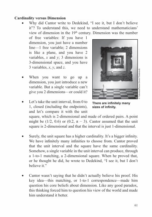
61

Cardinality versus Dimension • Why did Cantor write to Dedekind, “I see it, but I don’t believe

it”? To understand this, we need to understand mathematicians’ view of dimension in the 19th century. Dimension was the number of free variables: If you have 1 dimension, you just have a number line—1 free variable; 2 dimensions is like a plane, and you have 2 variables, x and y; 3 dimensions is 3-dimensional space, and you have 3 variables, x, y, and z.

• When you want to go up a dimension, you just introduce a new variable. But a single variable can’t give you 2 dimensions—or could it?

• Let’s take the unit interval, from 0 to 1, closed (including the endpoints), and let’s compare it with the unit square, which is 2-dimensional and made of ordered pairs. A point might be (1/2, 0.6) or (0.2, π − 3). Cantor assumed that the unit square is 2-dimensional and that the interval is just 1-dimensional.

• Surely, the unit square has a higher cardinality. It’s a bigger infinity. We have infinitely many infinities to choose from. Cantor proved that the unit interval and the square have the same cardinality. Somehow, a single variable in the unit interval can produce, through a 1-to-1 matching, a 2-dimensional square. When he proved that, or he thought he did, he wrote to Dedekind, “I see it, but I don’t believe it.”

• Cantor wasn’t saying that he didn’t actually believe his proof. His key idea—this matching, or 1-to-1 correspondence—made him question his core beliefs about dimension. Like any good paradox, this thinking forced him to question his view of the world and made him understand it better.

There are infinitely many sizes of infinity.

© V

alen

tinaP

hoto

s/iS

tock

/Thi

nkst

ock.

62

Lect

ure

8—C

anto

r’s In

finity

of I

nfini

ties

Dauben, Georg Cantor.

Dunham, Journey through Genius.

1. If cardinality doesn’t distinguish dimensions, what does?

2. What did Cantor mean when he wrote, “I see it but I don’t believe it”?

Problems

Suggested Reading

63

Impossible SetsLecture 9

This lecture will concentrate on a single paradox and the story of how it was eventually resolved—twice. In this lecture, you will learn about Russell’s paradox. It is profound, yet simple to state. It took decades

of work to resolve. It’s a story of dreams being repeatedly dashed with an ending that really surprised everyone. The entire lecture is devoted to this one paradox—its history, the mathematics it sparked, and the mathematicians whose lives revolved around finding a resolution to it.

Russell’s Paradox • In 1901, Bertrand Russell, British philosopher and mathematician,

observed a logical hole in Georg Cantor’s theory of sets.

• Some sets have the strange property that they are elements of themselves. They are self-containing. It’s really difficult to illustrate this with simple sets of numbers.

• Let’s take a weirder set: the set of all abstract ideas. Is that set an abstract idea? It certainly is abstract. Therefore, the set of all abstract ideas includes itself. It’s self-containing.

• Cantor proved that there are infinitely many sizes of infinity, so there are infinitely many sets of infinite sets. So, the set of all infinite sets is also self-containing. It’s one of the many things in itself. It contains many sets, one of which is itself. It’s self-containing.

• Most sets aren’t self-containing. The set of prime numbers is a set that contains numbers, not sets of numbers. So, this self-containing property is a very odd property.

64

Lect

ure

9—Im

poss

ible

Set

s

• Russell thought up a very ingenious set. Let’s call it R, the collection of all sets that are not self-containing. So, no set in R has the property that it is one of the elements in the set of itself. Is the set R self-containing? Let’s look at this in cases.

○ Case 1: R is one of the sets in R. Then, R is self-containing. It contains itself. But R consists of all the sets that are not self-containing. That’s a contradiction.

○ Case 2: R is not one of the sets in R. Then, R is not self-containing. But that’s exactly the condition all the sets in R satisfy—they’re all not self-containing. That’s also a contradiction.

• R is neither self-containing nor not self-containing. And that’s Russell’s paradox, a set of sets that aren’t self-containing. The key underlying problem is this: What is a set?

• What was a set to Cantor and others? It was anything you could describe in words. Cantor and Gottlob Frege subscribed to this idea. It’s something that now we call naïve set theory. We know that this is problematic. In Berry’s paradox, the smallest natural number not describable in English and fewer than 110 characters didn’t exist. Just because you can describe a set doesn’t mean that it exists.

Axiomatic Systems • Around 1900, there was a key question among mathematicians:

What is the correct foundation for mathematics? The goal was to be able to talk about numbers and sets—naturals, primes, power sets of sets.

• The problem is that there are so many paradoxical sets. We don’t want a set of sets that don’t contain themselves. We don’t want a set of all sets, a universal set. The thinking was to resolve this paradox by avoiding it. Such things wouldn’t be permissible as sets. Thus began the search for a set of axioms, or assumptions, that would create a foundation for mathematics. In the 1920s, David Hilbert pushed this idea and dubbed it Hilbert’s program.

65

• The most famous set of mathematical axioms goes all the way back to Euclid’s axioms for plane geometry. Euclid’s five axioms included statements like the following: One can connect any two points, and one can make a circle centered at any point with any positive radius. The fifth axiom, called the parallel postulate, was much more controversial. There are different versions of it, but it states that given any line and a point not on that line, one can construct a unique line through the point parallel to the line.

• The goals of any of these axiomatic systems were to avoid confusion. If we have an agreement on what we’re starting from, then we avoid confusion. We also wanted to clearly lay out the ground rules for the subject because the goal was always to establish a firm foundation for the enterprise. In Euclid’s case, it was geometry.

• Axioms should be consistent. You should not be able to prove contradictions. In addition, they should be complete. All true statements should be provable. If a statement is true, you should be able to prove it from the axioms and the logical rules within the system. Also, axioms should be minimal. If you could prove one of them using the others, then you should just omit it and not call it an axiom.

• Euclid’s axioms were great. They could prove many different theorems, including the Pythagorean theorem. Many of the things that you could prove in this system used the fifth axiom—but some didn’t.

• The big question for Euclid’s axioms was this: Is the fifth axiom redundant? Can you prove the fifth one from the first four? There are many statements that are equivalent to the fifth. If they are true, then the fifth one is true; if the fifth one is true, then they are true. But the world’s best mathematicians tried and failed to prove the fifth axiom, or anything equivalent to it, from the first four.

66

Lect

ure

9—Im

poss

ible

Set

s

• In the 1800s, Carl Friedrich Gauss, Nikolay Lobachevsky, and János Bolyai all independently figured out that if you change the parallel postulate, geometry still works. You take a line and a point, and there’s just one line through the point parallel to the line. What would geometry look like if there were no parallels through that point, or if there were more than one?

• The result is non-Euclidean geometry. Technically, you get non-Euclidean geometries, because these two different answers give you different geometries. If there’s no parallel through a point, you get what’s called elliptical geometry.

Theory of Types • If you want axioms for set theory (and for arithmetic)—the goal

being to define sets and avoid paradoxes—you have to be very precise and careful to avoid having multiple answers.

• German mathematician Gottlob Frege worked to write down axioms to finally construct a logical foundation for arithmetic and for set theory—really, for all of math. He did this in a series of important works, from 1879 to 1903.

• In 1903, Frege’s Basic Laws of Arithmetic (volume 2) was almost to press when Russell wrote to him and said that Frege’s axioms left his system open to what we now know as Russell’s paradox. Within his system, one could construct a set of all sets that did not contain themselves. Before he went to press, Frege realized that Russell’s objection was correct and hastily wrote an appendix with an incomplete modification.

• Ironically, a similar fate would await Bertrand Russell years later. Russell started picking up where Frege left off. Russell realized that the core of his paradox is this self-reference: R is the collection of sets that are not self-containing. Then, R may or may not be self-containing.

67

• In contrast, the set of prime numbers, P, is not self-referential. P is a collection of numbers. It can’t be self-containing because it’s not, itself, a number. P only contains numbers. There’s no self-reference, so there’s no problem.

• Russell and others—including Russell’s teacher, Alfred North Whitehead—worked to figure out axioms that avoided this sort of self-reference, and their answer is called the theory of types. Russell and Whitehead’s theory of types resolved Russell’s paradox. And it resolved some other paradoxes, but the solution was abandoned. More elegant solutions were found. And those are still used today.

Zermelo-Fraenkel Set Theory • By 1922, Ernst Zermelo and Abraham Fraenkel found a set of

axioms for set theory. Called ZF, for Zermelo and Fraenkel, this set of axioms is now accepted by the math world.

• How do they get around the paradoxes? It’s very careful, highly technical work with things like the axiom of regularity and the axiom schema of specification. Essentially, they’re figuring out rules so that sets can’t be too strange. There’s no set of all sets. There’s no Russell’s paradox.

• Zermelo and Fraenkel wrote out eight axioms, and they used them to prove many theorems. But they still couldn’t prove some things. For example, they couldn’t prove that if you have two sets, then the cardinality of one is greater than or equal to the cardinality of the other. This is obvious for finite sets, but it’s not obvious for infinite sets.

• Zermelo thought that this should be provable, but he couldn’t prove it with the eight axioms. They needed one more: the axiom of choice. The axiom of choice is one of the most controversial pieces of mathematics.

68

Lect

ure

9—Im

poss

ible

Set

s

• Imagine that you had 15 sets—for example, 15 baskets of fruit. None of them was empty. Can you create a set consisting of exactly one piece of fruit from each basket? If this were the physical world, there’s no problem. You’d just grab one piece from each basket and put it in your set. In the math world, that’s also not a problem. You can do that with the first eight axioms of Zermelo-Fraenkel theory.

• What if you have an infinite (countable) collection of sets? In the physical world, that’s a problem. You’d have to do some sort of super task. In the mathematical world, it’s also not provable from the first eight axioms. You need the ninth axiom, the axiom of choice. The axiom of choice says that you can do that.

• Imagine one basket at every natural number off to infinity. It’s fairly easy to create a new basket with something from baskets 1 through 100, but it’s harder to create a new basket with something from every single one of the infinitely many baskets. The axiom of choice says that you can do that. Oddly, the axiom of choice doesn’t tell you how to do it or what set you end up with.

• In fact, the axiom of choice says something even more. Imagine one basket, not at every natural number, but at every real number between 0 and 1 (uncountably many numbers). Can you create a new set with something from every basket? The axiom of choice says that you can always do it. Again, it doesn’t tell you how or what you end up with.

• There are many statements in mathematics that are equivalent to the axiom of choice. A statement S is equivalent to the axiom of choice if you assume S and the first eight axioms. Then, with those nine things, you can prove the axiom of choice. And if you take the first eight axioms and the axiom of choice, you can prove your statement S.

• There’s a very long list of famous mathematical theorems that are all equivalent to the axiom of choice, including the well-ordering

69

theorem, Zorn’s lemma, and Tikhonov’s theorem. And these statements are either all true, if you assume the axiom of choice, or all false, if you don’t.

• ZFC, Zermelo-Fraenkel with choice, is about set theory. But mathematicians talk about ZFC as if it is a foundation not just for set theory but also for arithmetic. And that’s a little strange, but there is a connection between a foundation for set theory and one for arithmetic.

• Can these nine statements that form the foundation for mathematics—Zermelo-Fraenkel with choice—prove all the statements we want? Surprisingly, no, they can’t. Self-reference and strange loops come out again to destroy that dream. It turns out that there’s no set of axioms that could possibly prove all of the true statements about arithmetic.

Moore, Zermelo’s Axiom of Choice.

1. Sets are defined with language (mathematical, English, Chinese, etc.). In any case, each language contains only finitely many symbols, and every definition has, for example, fewer than 10,000 symbols. If we assume that the real numbers are “well ordered” (a technical term that means, essentially, that they can be put in some order with some element first), then we can create a subset of the real numbers that is defined by a finite definition. What’s paradoxical about this set?

2. One way the Zermelo-Fraenkel axioms get around some paradoxes is the subtle axiom of regularity, requiring that every set X contains at least one element that doesn’t share any elements with X. How does this axiom imply that there is no set of all objects, no “universal set”?

Suggested Reading

Problems

70

Lect

ure

10—

Göd

el P

rove

s th

e U

npro

vabl

e

Gödel Proves the UnprovableLecture 10

Mathematicians love simplicity. Around 1900, their dream was to create a world of math that was cleanly split in two: true statements, which would all be provable from axioms, and false

statements, none of which would be provable from axioms. Kurt Gödel destroyed that dream with a single sentence; he found a statement that was true but not provable: “This statement is not provable.” It seems simple, but the details are far from it. In this lecture, you will learn how this strange loop with its seemingly simple bit of self-reference destroyed the dreams of many mathematicians but opened up a whole new world of mathematics.

The First Incompleteness Theorem • In 1928, Kurt Gödel attended a talk by David Hilbert in Bologna,

Italy, at an international math conference. Hilbert talked about some of the great unsolved problems. And he made an important distinction between statements that were true within a system and statements that were provable within that system. Hilbert’s program included the search for axioms that avoided paradoxes, such as Russell’s paradox, and could prove all of the known mathematical truths.

• In 1931, just three years after Hilbert’s talk, Gödel had proved that Hilbert’s program was impossible when he published On Formally Undecidable Propositions of Principia Mathematica and Related Systems I. It was an attack on Bertrand Russell and Alfred North Whitehead’s axioms in Principia Mathematica.

• This work contained Gödel’s first groundbreaking result: Gödel’s first incompleteness theorem, which basically says that any axiomatic system strong enough to include basic arithmetic will necessarily include a statement that is true but not provable within that system.

71

• In the world that Hilbert’s program would have ushered in, all mathematical statements would be divided into two kinds: true and false. The true ones—for example, 2 + 2 = 4—would all be provable from a few simple axioms, such as the Zermelo-Fraenkel with choice axioms. None of the false statements—such as 2 + 2 = 5—would be provable from these axioms. It would be consistent (no contradictions) and complete (all true statements would be provable).

• Gödel managed to encode, in mathematics, a version of this sentence: “This statement is not provable.” Its simplicity is as amazing as its depth, yet it hides great complexity.

• Why does this destroy Hilbert’s program? Let’s ask two questions about this sentence, usually called a Gödel sentence: Is it true? Is it provable in whichever axiom system you have?

• If it were provable, then you could use it to prove that the Gödel sentence is not provable because that’s what it says—it says that the sentence is not provable. If you’re in a consistent system, you can’t prove both a statement and its opposite. Therefore, the statement must not be provable. But if it’s not provable, then it’s true, because that’s what it says—it says that it is not provable. That’s correct.

• You can’t prove it. It’s a contradiction. Therefore, it must be true. Gödel showed that there’s no way to split up the world into true (all provable) and false (none provable). His statement was true but not provable. There must be some sort of gray area. The Hilbert program was dead. No perfect set of axioms for mathematics exists. Every such system has its flaws.

• Stating the Gödel sentence hides the real difficulty in Gödel’s work. The goal is to use the axioms of Principia Mathematica to encode the sentence within the language of the axiomatic system itself.

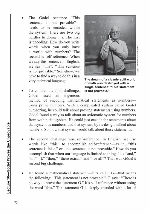
72

Lect

ure

10—

Göd

el P

rove

s th

e U

npro

vabl

e

• The Gödel sentence—“This sentence is not provable”—needs to be encoded within the system. There are two big hurdles to doing this. The first is encoding: How do you write words when you only have a world with numbers? The second is self-reference: When we say this sentence in English, we say “this”: “This sentence is not provable.” Somehow, we have to find a way to do this in a very technical language.

• To combat the first challenge, Gödel used an ingenious method of encoding mathematical statements as numbers—using prime numbers. With a complicated system called Gödel numbering, he could talk about proving statements using numbers. Gödel found a way to talk about an axiomatic system for numbers from within that system. He could just encode the statements about that system as numbers, and that system, by its design, talked about numbers. So, now that system would talk about those statements.

• The second challenge was self-reference. In English, we use words like “this” to accomplish self-reference—as in, “this sentence is false,” or “this sentence is not provable.” How do you accomplish that when our language is limited to things like “and,” “or,” “if,” “then,” “there exists,” and “for all”? That was Gödel’s second big challenge.

• He found a mathematical statement—let’s call it G—that means the following: “This statement is not provable.” G says: “There is no way to prove the statement G.” It’s self-reference without using the word “this.” The statement G is deeply encoded with a lot of

The dream of a cleanly split world of math was destroyed with a single sentence: “This statement is not provable.”

© D

igita

l Vis

ion/

Phot

odis

c/Th

inks

tock

.

73

mathematics, but it implies that the statement is not provable, and therefore, it must not be provable. And it says, “I am not provable,” and therefore, it must be true.

• Gödel’s ingenious method used the axiomatic system of Russell and Whitehead, which they had carefully constructed to avoid contradictions—such as Russell’s paradox—and constructed within that system a statement that showed that their axioms couldn’t prove everything that was true.

• You might think you see a way out of Gödel’s trap: He found a statement that the axioms couldn’t prove, so just include it as another axiom. Then, its proof would be easy.

• This objection is reminiscent of the common attack on Cantor diagonalization. If we find a real number that is not on the list of natural numbers, can we just add that as the first number on the list? The power of diagonalization, the Cantor argument, was that it covered every possibility. Cantor showed that if you put that number on the list, then you could just diagonalize the remaining list. He showed that there’s always something that’s not on that list. No 1-to-1 correspondence can ever be found.

• Gödel’s proof did the same thing for axioms that purported to give a foundation to arithmetic and the idea that they could prove every statement that was true. Gödel showed not only that Russell and Whitehead’s list of axioms was missing something in the sense that there would be some statement that would be true but not provable, but he also showed that every axiom system would have the same problem.

• Every system has a Gödel sentence. You add a new axiom, and Gödel’s process would find another unprovable statement that was true. Gödel says that this task of finding exactly the right axioms is a Sisyphean task—it won’t end well.

74

Lect

ure

10—

Göd

el P

rove

s th

e U

npro

vabl

e

• This is an amazing mathematical achievement, one that changed the course of the field. Things that everyone had believed to be possible were suddenly proved to be impossible. Unlike with Cantor’s work on infinity, there was no controversy. People quickly realized the importance and the correctness of Gödel’s work. For mathematicians, the way things seemed to be just all of a sudden changed. It was turned into an illusion.

The Second Incompleteness Theorem • In 1928, young Gödel was at Hilbert’s talk, in which Hilbert

optimistically claimed that others had proved that number theory and analysis were consistent and didn’t contain any contradictions. Within three years, Gödel proved Hilbert to be wrong. That was the second incompleteness theorem.

• In musical terms, the second theorem represents a coda to his 1931 paper, a mathematical bonus to an already groundbreaking opus. The main theorem was the first incompleteness theorem: Every axiomatic system that contains basic arithmetic must contain a statement that is true but unprovable.

• What does the second incompleteness theorem say? Basically, there are many things an axiomatic system can prove—one that includes basic arithmetic. Can it prove that an axiomatic system can’t prove any contradiction? The second incompleteness theorem says that it can’t do that—that it can’t prove its own consistency.

• It actually says something slightly more specific: If a system does include a proof of its own consistency, then the system is, in fact, inconsistent. Gödel proves this in yet another ingenious way.

• First, he proves the following statement within the axiomatic system, called statement A: “If the system is consistent, than the Gödel sentence is provable.” He has already proven earlier in the paper that the Gödel sentence is not provable.

75

• If the system could prove its own consistency, then the statement A, which is an if-then statement, would have its hypothesis proven true. And, therefore, the conclusion would be proven. But we know that the conclusion can never be proven. The conclusion says that the Gödel statement is provable. Thus, no system can prove its own consistency.

• Gödel’s work is incredibly complicated. It contains many, many layers. But there are a few key points to understand. Gödel used self-reference, which has been a key in many paradoxes, to show us surprising results about axiomatic systems. In doing so, he opened up new areas of study.

• Gödel had an incredible obsession with systems of rules, how they fit together, and what their implications were. When it comes to mathematics, his obsession with rules gave us the stunning results that revolutionized the field.

Nagel and Newman, Gödel’s Proof.

Smullyan, Satan, Cantor, and Infinity.

1. Why doesn’t each of the following sentences serve as a way to prove Gödel’s incompleteness theorem?•• This sentence is provable.

•• This sentence is false.

Suggested Reading

Problem

76

Lect

ure

11—

Votin

g Pa

rado

xes

Voting ParadoxesLecture 11

Politics is full of paradoxes. Many of them are just issues that we disagree strongly about, but a few have a mathematical basis. In this lecture, you will learn about election paradoxes. American economist

Kenneth Arrow’s theorem of voting systems proved that if you’re looking for a voting system that satisfies four sensible-sounding criteria, you’re out of luck. No fair voting system exists. Before learning about Arrow’s theorem, proving that every one of these voting methods is flawed, you will be introduced to these different kinds of voting systems.

Voting Methods • Samuel Tilden, Grover Cleveland, and Al Gore all would have won

their respective presidential elections had the Constitution relied on the popular vote instead of on the electoral college. The U.S. presidency isn’t decided by majority vote (more than half of the votes) or even by plurality vote (the candidate with the most votes). Instead, each state elects electors, mostly in a plurality manner within the state, and the winter takes all in that state. Then, those electors vote in the electoral college.

• The impact of this particular election model on modern American politics is difficult to overstate. Billions of dollars are poured into a handful of swing states, with candidates hoping to get to the magical number of 270 electoral votes that are needed to win. The electoral college can produce counterintuitive results.

• So, a candidate could lose the popular vote but win the presidency. How badly could he or she lose the popular vote? A candidate in a two-person race could get just enough votes to win just enough of the least populous states. The least populous states have more weight; the smallest states get a minimum of three electoral votes.

77

Even if a candidate didn’t get a single vote in the most populous states, he or she could get to 270 electoral votes with less than 1/5 of the people voting for him or her.

• Different political scientists and mathematicians have devised different voting methods. Few of them are as convoluted as the U.S. presidential system.

• If you have just two options, majority rules is the only fair system. This is a mathematical theorem called May’s theorem.

• When you have more than two options, voting methods start to become increasingly complicated. Some indication of why they get so complicated is the strategic voting that we’ve seen in some presidential elections. In 2000, websites popped up where people could trade their votes. Basically, voters avoided their least-favorite option while still getting a vote counted for their favorite option—it just wasn’t their vote. An ideal voting system would try to avoid this sort of strategic voting.

• Another reason that three options and more get a little confusing has to do with the fact that choices can be cyclic. Suppose that you have three voters and three options. Instead of politics, think of three friends—Rebecca, Steve, and Tim—choosing a restaurant to go to, from three choices: Brazilian, Chinese, and Danish.

• Suppose that Rebecca prefers Brazilian to Chinese to Danish, in decreasing order of preference. Steve prefers Chinese to Danish to Brazilian, and Tim prefers Danish to Brazilian to Chinese. Should they get Brazilian food? Steven and Tim both prefer Danish to Brazilian, so they shouldn’t do that. What about Danish food? No, Rebecca and Steve both prefer Chinese to Danish. What about Chinese food? No, Rebecca and Tim both prefer Brazilian to Chinese. And that completes the cycle: Brazilian beats Chinese, Chinese beats Danish, and Danish beats Brazilian.

78

Lect

ure

11—

Votin

g Pa

rado

xes

• This is the Condorcet paradox, named after 18th-century French mathematician Marquis de Condorcet. This doesn’t always happen, but if one candidate beats all the others in pair-wise matchups, that’s called a Condorcet winner.

• The Condorcet voting method is that if there is a Condorcet winner (who wins all of the pair-wise matchups), then that should be the winner in your voting system. In this case, when we have these cycles, there’s no resolution. Every option is in exactly the same situation. You have to accept that preferences can form these cycles.

• If you have three or more candidates, one way to settle things is to hold runoff elections. After an initial vote, where each voter gets to vote for his or her top choice, the last candidate (or maybe all but the top two) is dropped, and the remaining candidates compete in a runoff.

• This requires an additional voting day, unless you do something called an instant runoff. And if you want to do that, you have to ask voters to rank all of the candidates. Initially, only their top choices are counted. If there’s no majority, then some candidates on the bottom are dropped and the votes are retabulated. The voter’s ballots count for the top choice that hasn’t been dropped.

• Another way to decide these sorts of things is with approval voting, in which each voter votes for as many options as he or she wishes—for all the ones he or she approves of. One way to think of approval voting is that each voter gives one point to any or all of the acceptable options, and then the option with the most points wins.

An election winner often owes thanks to the system—a different system might have chosen a different winner.

© T

hink

stoc

k Im

ages

/Sto

ckby

te/T

hink

stoc

k.

79

• There is a variant of approval voting, which voting theorists call Borda count, in which instead of treating all of the approved options equally, voters rank all of the possible options, and the last one on their list gets 0 points. The next-to-last option gets 1 point, the next one higher on the list gets 2 points, and so on, all the way up their list. Then, you add up everyone’s totals, and the option with the most points wins.

• Agenda voting is a voting system that sounds strange but is used surprisingly widely. You establish an agenda and order the options. If you had options A through D, your agenda might read D, then B, then C, then A. Then, you do pair-wise voting, like in a tournament, except that you have byes in this tournament. First, it’s D versus B. The winner of that matchup takes on C. The winner of that matchup takes on A. Note that A only has to win one race to win the election, whereas D has to essentially beat everybody else to win the election.

• In such a system, whoever controls the agenda has immense power. It turns out that most legislatures work like this. Agenda voting is sequential pair-wise voting. It allows for strategic voting, which is not ideal.

• Another voting system is approval voting, in which you get to vote for all of the candidates you approve of. With this system, we don’t have enough data from polling to know if people approved of just their top choice or their top two.

• Often, the voting system affects the outcome, and some of these are subject to strategic voting. The main point is that an election winner often owes thanks to the voters, of course, but also to the system. A different system might have chosen a different winner.

Arrow’s Voting Method • Which voting method is best? Economist Kenneth Arrow provided

the answer to this question. No voting method does what we think it should.

80

Lect

ure

11—

Votin

g Pa

rado

xes

• Kenneth Arrow described a few conditions that an ideal voting system should have, ranging from simple to more complicated. A simplified version of four of these conditions is as follows.

○ Non-dictatorship: More than one person’s vote counts.

○ Universality: Anyone is allowed to order the candidates in any rational way, but it must be noncyclic. (No single person should prefer A to B, B to C, and C to A.) The results of voting should be a complete ranking of all of the options once you get everybody’s votes together.

○ Unanimity: If everyone prefers A to B, then A should beat B (or at least be ahead in the final rankings).

○ Independence of irrelevant alternatives: If A defeats B when C is in the race, then A should still defeat B if C drops out. Arrow argued that independence of irrelevant alternatives was a common sense and a desirable quality. The U.S. presidential elections fail this test.

• Arrow’s theorem says that no voting system has all four of these conditions. It’s not possible. Every voting system violates at least one of these conditions.

• What do we make of this theorem today? There is this romantic view of democracy as establishing the will of the people. Arrow’s theorem says that there is no way for elections to determine the will. It’s more complicated than that. Examples of different voting systems show that which system you choose definitely matters.

• Arrow’s theorem shows that no system reaches “fairness” as you might think. Other researchers went on to study the different flaws and susceptibilities of different systems to strategic voting.

81

• The mathematical proof of Arrow’s theorem is an interesting one. He starts by assuming that a voting system has all the conditions except the dictatorship condition. Then, if it’s not a unanimous vote between A and B, he finds a pivotal voter—a voter who, if the preferences changed, would swing the election from A to B (or the reverse). Finally, he uses that to prove that the pivotal voter is actually a dictator—one who has complete control over the election. It’s interesting to see how these three conditions lead to this last step.

The Chair’s Paradox • The chair’s paradox is a strange voting paradox. In many

organizations, the way to break ties is to allow the chair to break the tie. Sometimes the chair is not a member of the body. For example, the Vice President breaks ties in the U.S. Senate. But sometimes, the chair is also a voting member.

• You would think that being chair would give you more power, and in some cases, that’s true—deciding the agenda in agenda voting, for example. But amazingly, that’s not always true. There are cases where being chair makes it less likely that you’ll get the outcome you want.

• The chair’s tie-breaking power could cause other voters to vote differently, and the end result could be that the chair gets his or her least-preferred option. Therefore, the chair would be better off giving someone else the power of being chair.

• This chair’s paradox was first written about in 1958 by Robin Farquharson, a South African game theorist. As with all of the other oddities of voting, his paradox shows us how much is hidden behind the seemingly simple act of voting.

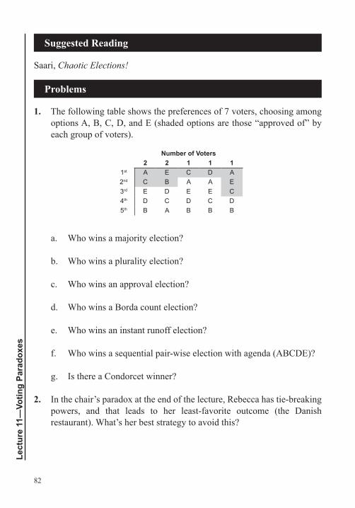
82

Lect

ure

11—

Votin

g Pa

rado

xes

Saari, Chaotic Elections!

1. The following table shows the preferences of 7 voters, choosing among options A, B, C, D, and E (shaded options are those “approved of” by each group of voters).

a. Who wins a majority election?

b. Who wins a plurality election?

c. Who wins an approval election?

d. Who wins a Borda count election?

e. Who wins an instant runoff election?

f. Who wins a sequential pair-wise election with agenda (ABCDE)?

g. Is there a Condorcet winner?

2. In the chair’s paradox at the end of the lecture, Rebecca has tie-breaking powers, and that leads to her least-favorite outcome (the Danish restaurant). What’s her best strategy to avoid this?

Suggested Reading

Problems

Number of Voters2 2 1 1 1

1st A E C D A2nd C B A A E3rd E D E E C4th D C D C D5th B A B B B

83

Why No Distribution Is Fully FairLecture 12

The mathematics of apportionment comes up anytime one has to share a discrete resource—something that can’t be split up into fractional pieces—among different groups. The classic case is like

the U.S. House of Representatives: Different groups have to send people to a representative body, and the representation is based on population. The key reason for the mathematical complexity is that representatives are discrete; you can’t have 3.5 members from one state. Apportionment is fraught with paradoxes. Unfortunately, a theorem proved in 1982 shows that these paradoxes can’t be avoided.

Apportionment • Imagine a country with only 60 people in 3 states—A, B, and C—

with a legislature of 13 people. The population of these 3 states might be as follows: A has 25 people, B has 20, and C has 15. How many representatives should each state get?

• If you express their populations as a percentage of the whole country, A has 42%, B has 33%, and C has 25%. They should get that percentage of the seats. That would be 5.42 seats, 4.33 seats, and 3.25 seats. This is the fundamental problem of apportionment: You can’t have fractional representation like that.

• How should we deal with these fractional parts? How do we distribute this discrete resource, where only integer values are allowed, when the “fair” way would involve non-integers? That number—the non-integer, fair or proportional distribution—is called the standard quota.

• In the example, if we add the standard quotas, we get exactly the number of representatives: 13. To get an integer number of representatives, we have to round. If we round down, we have too

84

Lect

ure

12—

Why

No

Dis

trib

utio

n Is

Ful

ly F

air

few representatives: 12. If we round up, we have too many: 15. If we round to the nearest integer, sometimes we have too many and sometimes too few, but in this case, we have too few: 12.

• One of the first desired properties of a system is called the quota rule. The number of representatives a state ends up getting should be the standard quota either rounded up or rounded down.

• It would be very strange if you had a standard quota of 5.4—where you would, in an ideal world, get 5.4 representatives—but ended up with 7 seats (too many) or 4 seats (too few). If your standard quota is 5.4, you should end up with either 5 or 6 seats.

• An apportionment system that violates this quota rule would seem strange. The standard quota is the fairest, but it’s not an integer. If you didn’t get either the rounded-up or rounded-down number, that seems unfair. But the method currently used in the United States to apportion U.S. House of Representatives seats sometimes violates the quota rule.

• Another key number when it comes to apportionment is the standard divisor, which is the number of people per representative. In the example, there were 60 people and 13 representatives. The standard divisor is 60 ÷ 13, which is about 4.61. The units are people per representative. The standard divisor is roughly how many additional people a state needs in order to get an additional representative.

• The standard divisor and the standard quota are related. The standard quota is the state population divided by the standard divisor. The population is usually fixed, and if it’s fixed, then if the standard divisor increases, the standard quota decreases. If the standard divisor decreases, then the standard quota increases.

Apportionment Systems • Alexander Hamilton developed a method of apportioning U.S.

House seats. First, we calculate each state’s standard quota, and then we initially assign seats by rounding down. If we have more

85

seats to assign—in our example, we have 13 seats to fill, but only 12 are assigned so far—then we look at the fractional part of the standard quota and assign any remaining seats to the states with the largest fractional parts until we’re out. In our case, the largest fractional part goes to state A, which is 0.42, so state A gets the last seat.

• Hamilton’s method satisfies the quota rule by design. Every state either gets its standard quota rounded down (the initial number of seats) or rounded up (if its fractional part is large enough).

• President George Washington didn’t like the results of Hamilton’s method. As a result, in 1792, he issued the first veto by a U.S. president to veto this method. Instead, he turned to a method devised by Thomas Jefferson.

• Jefferson’s method starts out very similarly. We calculate the standard quota, but we also calculate the standard divisor. We round down the standard quotas. If we have the right number, then we’re done. But if we have too few, instead of looking at the fractional parts, we replace the standard divisor with a (lower) modified divisor and keep lowering that until the right number is reached.

• In our simple 3-state case, the standard divisor is about 4.62 people per representative. If we keep rounding down the standard quotas, it gives us 12 seats. We need 1 more, so we keep lowering the standard divisor (fewer people per representative).

• When we round down all the way to 4.5 people per representative, we still have the same result: 4.3. We keep going until we get 4.17 people per representative. Then, when we recalculate the quotas, state A gets the additional seat. The result is the same as the result using Hamilton’s method, but it’s for a different reason.

• In 1792, rather than having to try to override Washington’s veto of Hamilton’s method, Jefferson’s method was used. The loser in this case was Delaware. With Hamilton’s method and looking at its

86

Lect

ure

12—

Why

No

Dis

trib

utio

n Is

Ful

ly F

air

fractional parts, its standard quota of 1.61 was rounded up to 2. But using Jefferson’s method, using the modified divisor, Delaware only got 1 house seat—1 fewer seat. The U.S. Constitution at the time said that the number of representatives shall not exceed 1 for every 30,000 people, and giving Delaware 2 would exceed that limit.

• Jefferson thought that he had ended the debate about apportionment methods. Jefferson’s method was only used in the United States through the 1840 census. Since then, other variations of apportionment methods have been used.

The Alabama Paradox • The Alabama paradox, which was first noticed for Rhode Island,

has to do with changing the number of seats in the House. The U.S. Census Bureau used Hamilton’s method. It was looking at the largest fractional parts.

• Ulysses Mercur, a Pennsylvania congressman, noticed that when the size of the House went from 270 to 280 seats, Rhode Island went from having 2 seats to 1 seat. Why would one state lose a seat when there are more seats to go around?

• Mercur’s discovery didn’t get widely noticed until about 10 years later. Following the 1880 census, C. W. Seton, the chief clerk at the Census Bureau, noticed the same oddity Mercur had found: With 299 seats, Alabama got 8 seats, but with 300 seats, Alabama only got 7 seats. Seton used this to argue against Hamilton’s method in a letter to Congress.

• After the 1900 census, the problems of Hamilton became even clearer. Calculating apportionments for all House sizes from 350 to 400, the size of Maine’s delegation switched between 3 and 4—5 times!

• Why does the Alabama paradox happen? Why is it that when you add 1 seat to the House, it isn’t the case that just 1 state gets a new seat? Sometimes 2 states get additional seats and another state loses a seat—Alabama loses a seat.

87

• In moving from 299 to 300, you can calculate the old quotas and the new ones. With the old numbers, Alabama has a fractional part that edges out Texas and Illinois. With the new numbers, both Texas and Illinois have fractional parts that are higher than Alabama’s.

• When you use Hamilton’s method, the seats added—where we round to the standard quota—shift from Alabama to Texas and Illinois. Instead of just awarding the new seats to a single state, 2 states—Texas and Illinois—both get new seats, and Alabama loses one. The discovery of the Alabama paradox was the end of the Hamilton method.

The New State Paradox • A few years later, the Census Bureau

noted another flaw: the new state paradox. In 1907, Oklahoma joined the union. By size, it matched states with 5 representatives in the House, so it made sense to increase the number of seats from 386 to 391.

• The new system they moved to was called Webster’s method. We round all of the quotas to the nearest number and then adjust the standard divisor up or down until we get the right number of seats when we round. Webster’s is similar to Jefferson’s, but the rounding is to the nearest number, not always rounding down.

• Webster’s method avoided the Alabama paradox and the new state paradox, but there were other problems. In rare cases, Webster’s method would violate the quota rule. Sometimes the number of seats was not equal to the standard quota either rounded up or down. It was further away.

Jefferson thought that he had ended the debate about apportionment methods, but his method was only used in the United States through the 1840 census, after which other methods were used.

© g

nage

l/iSt

ock

Edito

rial/T

hink

stoc

k.

88

Lect

ure

12—

Why

No

Dis

trib

utio

n Is

Ful

ly F

air

• Webster’s method didn’t last long because of the work of a Census Bureau statistician named Joseph Hill, who brought a different perspective to apportionment. Instead of allocating the seats one at a time, Hill suggested focusing on the per capita representation. If state A with 2 million people has 5 seats, it has a per capita representation of 5 divided by 2 million, or 2.5 seats per million people. If state B has 7 million people and 18 seats, it has 18 divided by 7, or 2.571, seats per million. So, state B has greater representation.

• What if state B gave 1 seat to state A? Then, state A would have 6 divided by 2, or 3, seats per million. But B would have 17 divided by 7, or 2.429, seats per million. That’s a bigger gap. So, the switch made things less fair. The core of Hill’s idea is to find a distribution so that no switches make things more fair.

• Hill found a mathematician to help implement his idea. Harvard mathematician Edward Huntington proved in 1921 that such a method exists and gave a way of computing it. The Huntington-Hill method is still used today for U.S. House apportionment. It has been used since 1940.

• The key innovation of the Huntington-Hill method is when to round up the standard quota versus rounding down. Generally, if the standard quota is between n and n + 1, you compare the fractional part with the geometric mean of n and n + 1:

( )+n n11.

Sometimes a modified divisor is also needed.

• The result of this is that states are much more likely to round up. This accomplishes Hill’s goal, because no switching makes per capita representation any more even. It also manages to avoid the Alabama paradox and the new state paradox. Unfortunately, like Webster’s method, it sometimes violates the quota rule.

89

The Population Paradox • In the United States, there is a regular census every 10 years.

Afterward, we go through a period of reapportionment. It would be reasonable to assume that if you gain population, you might lose a seat—it’s possible that other states gained population even faster than you did. But it would be weird if your state gains in population and loses a seat, and at the same time, a neighboring state loses population but gains a seat. That is the population paradox.

• Under some forms of apportionment, it’s possible to have one state gain in population and another lose in population, but have the first state lose a seat and the latter gain a seat. In fact, the seemingly simple quota rule—that you have to round either up or down but not pass the next natural number—is surprisingly strong. No method that satisfies the quota rule can possibly avoid the population paradox.

• In other words, no matter what apportionment system you use, if it satisfies the quota rule, one state will gain in population but lose seats, and another state will lose population but gain a seat. Every method that satisfies the quota rule must sometimes exhibit this population paradox. This is a stunning mathematical result. It’s due to Balinski and Young, who proved it in 1982.

Balinski and Young, Fair Representation.

1. If no method avoids all of the paradoxes, why do we use the Huntington-Hill method?

2. How are the geometric mean ( ab ) and the arithmetic mean ((a + b)/2) related?

Suggested Reading

Problems

90

Lect

ure

13—

Gam

es w

ith S

tran

ge L

oops

Games with Strange LoopsLecture 13

In this lecture, you will be introduced to mind-bending paradoxes in games and game theory. As with other paradoxes, these puzzles and games help us understand the world around us. As you will learn,

mathematics has a way of being useful in the real world, even when it wasn’t designed that way. With some puzzles, when you fix your flawed intuition, you become a better thinker. In the end, all of these mind-bending puzzles help us become better thinkers.

The Pirate Game • Suppose that there’s a group of 5 pirates, and they are smart,

greedy, and bloodthirsty. But they’re greedy before they’re bloodthirsty. If they need to split up a bounty, they order the pirates by seniority, oldest to youngest, and then the newest one proposes a distribution plan. Then, the pirates vote on the plan. If the plan gets a majority—more than half—they implement the plan and sail away. If the vote fails, the newest pirate, the one who proposed the plan, walks the plank.

• The next most junior pirate then has to propose a distribution plan. And the process continues until somebody’s plan gets voted in with the majority of the votes. Then, they divide up the booty and sail away.

• One day, they find a treasure of 100 gold coins. Would you rather be the newest pirate or the senior one, who gets to vote on all of the other plans but doesn’t get to propose one? With puzzles like this, it’s best to start from small cases and work up.

• With only 2 pirates, a majority of the pirates is the same as unanimity. But what will happen? The elder one won’t agree to anything. Even if pirate 2, the younger one, proposes to give everything to the elder one, the elder one is bloodthirsty. He gets

91

to walk away with the entire booty anyway. He might as well get the booty and see pirate 2 walk the plank. So, if it’s just 2 pirates, the senior pirate (pirate 1) gets everything, and the junior pirate (pirate 2) dies.

• With 3 pirates, pirate 2 is thinking, whatever pirate 3, the youngest, proposes, if it fails, I’m going to die—because then we’re left with 2 pirates, and we’ve figured out that scenario. So, pirate 2 will vote yes to anything. Pirate 3 knows this. Pirate 3 is greedy, and he can take all of the gold for himself.

• Pirate 3’s proposal is all 100 pieces of gold for himself and none for either pirate 1 or 2. They vote. Pirate 3 votes yes. Pirate 2 votes yes, and pirate 1 doesn’t matter. At least 1 and 2 escape with their lives, but they don’t get any gold.

• With 4 pirates, pirate 3 is thinking, I’m going to vote against everything—because if the plan goes down and pirate 4 dies, I’ll get everything. Pirates 1 and 2 realize that if the plan is voted down, then they get to watch pirate 4 walk the plank. But they’re not going to get any gold when they get down to just 3 pirates.

• So, pirate 4 has to find a plan that gets 3 votes, or he’s dead. Pirate 4 thinks, there’s no way for me to improve the outcome for pirate 3, so I can’t get his vote. But I can buy the votes of pirates 1 and 2 and take advantage of their greediness. So, pirate 4 proposes the cheapest bribe that will work: 98 gold coins

The pirate game is a counterintuitive conundrum with a surprising result.

© R

uben

Lem

ieng

re/H

emer

a/Th

inks

tock

.

92

Lect

ure

13—

Gam

es w

ith S

tran

ge L

oops

for himself, one gold coin each for pirates 1 and 2, and none for pirate 3. They vote. Pirates 1, 2, and 4 vote yes. Pirate 3 votes no. They all get to live, but pirate 3 gets no gold coins.

• With 5 pirates, pirate 4 will vote no, unless pirate 4’s plan beats their haul for 4 pirates. Pirate 5 is looking for a plan that would get at least 3 votes but save as much gold for himself as possible. Pirate 5’s proposal is 97 gold coins for himself, 1 for pirate 3, and 2 either for pirate 1 or pirate 2. For either one of them, the 2 gold coins would be better than the 1 gold coin he would have gotten if they were down to just 4 pirates.

• They vote. Let’s say that pirate 1 gets the 2 gold coins. Pirate 1 votes yes (2 coins are better than 1). Pirate 3 votes yes (1 coin is better than nothing). Pirate 5 votes yes. The most junior pirate walks away not only with his life, but with almost all the gold. It’s a counterintuitive conundrum with a surprising result.

The Two Envelopes Problem • Think of a game show. The host welcomes you and shows you

two envelopes, A and B. One envelope has an unknown amount of money, and the other envelope has twice as much. You get to pick. You can’t tell them apart. You pick envelope A.

• The host says, “You have envelope A—I’m not going to take it away. But envelope B might have twice as much. I’ll give you one chance. Do you want to switch envelopes and take home what’s in B?” You might think that it doesn’t matter, because you randomly chose A.

• So, 50% of the time, the other envelope has twice as much money, and 50% of the time, the other envelope has half as much money. Let’s assume that there are $x in envelope A. That means that there are either $2x or $x/2 in envelope B.

• If you stick with A, then you definitely get $x. If you switch to B, then half of the time you’ll get $2x and half of the time you’ll get $x/2.

93

• We can calculate the expected value of envelope B by taking the probability times the payoff and add all of those up: On average, 1/2($2x) + 1/2($x/2) = $x + $x/4 = $(5/4)x. So, if you switch to B, then on average, you get $5/4x, or $1.25x. Switching to B gets you 25% more money, on average.

• Suppose that while you got envelope A, the host handed envelope B to somebody else. That other contestant does the same calculation, thinking that switching to A gets him or her 25% more money. But both of you can’t be right. One person has the big pot; the other has the small pot.

• Another way to think of this is if you switch, then you could make the argument again that switching back will give you 25% more money. You could keep getting more and more money by switching envelopes. But, of course, that can’t be true. This is a true paradox.

Newcomb’s Paradox • In Newcomb’s paradox, devised by physicist William Newcomb,

someone hands you 2 envelopes, A and B. A is open, but B is closed. A says it contains $1000. You find out that B contains either $1 million or nothing. You choose both envelopes or just envelope B, the closed one.

• The twist is that the game is hosted by an all-knowing predictor—we’ll call him Neil—who predicts, without errors, what any human will do. Before Neil stuffs the envelopes, he does this as follows: If he predicts that you’re going to open just B, he puts $1 million in envelope B. If he predicts that you’ll open both envelopes, he puts nothing in B.

• Do you take both envelopes, or do you take just B? Both of these choices have really good arguments. If you take envelope B, Neil would have predicted that you would take only envelope B, and Neil would have put $1 million in envelope B. You’ll get $1 million.

94

Lect

ure

13—

Gam

es w

ith S

tran

ge L

oops

• But the envelopes are in your hands. The predictor can’t change what’s in them. You know that envelope B either has $1 million or $0. If you take just B, you get that money. But if you take both envelopes, you get whatever is in B plus $1000 more. If you take both envelopes, you automatically get more money, or the same.

• You get more money if you take both. But if you take both, then the predictor would have predicted that you would take both and would have put $0 in B, and you’ll end up with just $1000. So, you should take just B and earn $1 million. But then you’ve left $1000 in A, and that could have been yours. It’s certainly a strange loop that you’re in.

• There are two conflicting ways of deciding this. One is to calculate the expected value using the predictor’s 100% accuracy. But the other is some sort of dominance principle: If one option is always better, then you should take that option.

• These two ways of thinking are connected by a twist: Dominance says to take both, but the predictor says that if you take both, then B will contain $0. So, you avoid B, containing $0, and take just B. Then, the predictor—the twist—says that B will contain $1 million. But then dominance says that you should take both, and you get $1000 more. You just go around and around.

• There is something hidden in these statements that’s self-contradictory. Predictions that predict the future, where the event depends on the prediction, is a recipe for strange loops—for weird contradictions. In fact, the existence of a predictor is problematic. It’s difficult to make predictions, especially about the future.

The Puzzle of the Blue-Eyed Islanders • There are 100 inhabitants on an island, and they all have blue eyes.

There are no mirrors on this island, and nobody knows his or her own eye color. In fact, nobody ever talks about eye color, because it’s taboo.

95

• One boat docks on the island every day and leaves at noon. The odd rule is that if you ever learn your eye color, the next day, you must hop on the boat and leave forever.

• Years go by, and nothing happens. But one day, an explorer from a neighboring island arrives, and there’s a big party to welcome him. After dinner, he addresses everyone: “Where I come from, we all have brown eyes. Standing here, I look out and see someone with blue eyes.”

• What happens on the island after that? Our intuition says that it shouldn’t change anything. The visitor didn’t say anything that the islanders didn’t already know. They all knew that at least 99 people had blue eyes, because they could see everyone else.

• From the pirate problem, we know that we should start small. If there’s just one islander and the visitor says, “I see blue eyes,” then that’s definitely new information for that one person. The new information in this case is that there are blue eyes on the island. So, the next day, that one islander would have to leave.

• With two people, the visitor says, “Someone has blue eyes.” The next day, nothing happens. And that gives both islanders new information. Consider that you are one of the islanders: If you had brown eyes or any other color, then the other islander wouldn’t know of any blue eyes on the island. The other islander would have thought that he or she must be the one with blue eyes and would have left on day one. And that didn’t happen. So, that means it’s not true that you don’t have blue eyes. You must have blue eyes. So, on day two, you have to get on the boat.

• Interestingly, every islander does this same thinking if there are two people with blue eyes. So, the other islander does the same thinking, and on day two, both islanders get on the boat and leave.

96

Lect

ure

13—

Gam

es w

ith S

tran

ge L

oops

• Before the visitor, everyone knew there were blue eyes on the island. Everyone (the two people there) didn’t know that everyone knew there were blue eyes on the island. The visitor’s new information is this: Everyone knows that everyone knows there are blue eyes on the island.

• Jumping ahead to 100 people, nothing happens for 99 days, but on day 100, all the islanders meet at the dock and leave. For the 100 people, the new information the visitor gave them was that everyone knows that everyone knows that everyone knows that everyone knows that … , 99 times, someone has blue eyes: (Everyone knows that)99 someone has blue eyes.

• The underlying idea is common knowledge: Knowledge is common knowledge if not only does everyone know it, but everyone knows that everyone knows it … : (Everyone knows that)n (piece of knowledge) for any natural number n. This concept is important in game theory.

The Prisoner’s Dilemma • The prisoner’s dilemma, proposed by Merrill Flood and Melvin

Dresher, is a standard example in game theory. Suppose that there’s a pair of criminals being questioned—separately. The cops don’t have enough evidence, so they’re looking for one of the two to roll. Each prisoner has a choice: deny involvement or rat out the other.

• These choices have consequences for both suspects. If they both deny the crime, they each serve 1 year. The total served would be 2 years, 1 year each. If one denies but the other confesses, the confessor goes free, and the denier gets 3 years, resulting in a total of 3 years served. If both of them confess, they each get 2 years, so the total served is 4 years.

• Collectively, it’s less time served if they both deny the crime. But put yourself in the shoes of one of prisoner 1. There are two cases to analyze: Prisoner 2 will either deny or confess. If prisoner 2 confesses, then you’re better off confessing (2 years versus 3

97

years). If prisoner 2 denies the crime, then you’re also better off confessing (0 years versus 1 year). No matter what your accomplice does, you’re better off confessing.

• But you know that prisoner 2 makes the same calculation. The end result is that you both confess. You both serve 2 years—4 years total. But if you had both denied, you would have gotten 1 year each, for 2 years total. That’s the conundrum. Both prisoners are greedy, and because of their greed, they collectively get the worst-possible outcome.

• If you play the prisoner’s dilemma repeatedly—sometimes called an iterated prisoner’s dilemma—it becomes interesting. Many complicated strategies are possible, but the winning strategy is called tit for tat: In the first game, you cooperate by confessing. In the next game, you do what your opponent did the last time. If your opponent chose to cooperate, then you cooperate, too. If your opponent chose to compete, then you compete, too.

Dawkins, The Selfish Gene.

Gardner, Aha! Gotcha.

Stewart, Math Hysteria.

1. The following is a variant of the blue-eyed islander puzzle. Suppose that there are 60 blue-eyed people and 40 brown-eyed people on the island, and the visitor says, “It’s interesting to see both brown and blue eyes in your inhabitants.” What happens?

2. Return to the pirate puzzle (smart, bloodthirsty, greedy pirates, with the youngest proposing a way to divide loot and walking the plank if the plan doesn’t get a majority). How do the strategies change if a tie vote is good enough to approve a plan?

Suggested Reading

Problems

98

Lect

ure

14—

Losi

ng to

Win

, Str

ateg

izin

g to

Sur

vive

Losing to Win, Strategizing to SurviveLecture 14

In this lecture, you will learn about more game-based paradoxes, including the unexpected exam paradox, Parrondo’s paradox, and hat problems. As you will learn, self-reference is at the heart of the unexpected exam

paradox. In Parrondo’s paradox, you will discover how putting together two losing games might result in a win. Hat problems are interesting mind-bending puzzles, and it’s surprising how effective strategies can be. Strategies that deal with infinitely many hats are extremely counterintuitive, showing that infinity is a little stranger, and the axiom of choice is more powerful, than you might think.

Unexpected Exam • A logic professor walks into his class on a Friday. “We’re going to

have an exam next week, but I haven’t decided what day. You’ll walk into class, and all I can tell you is that the exam will be a surprise—unexpected. Be sure to study over the weekend.”

• Before the students leave, the best student speaks up: “I don’t think we have to study at all. You can’t wait until Friday for the exam. Then, we’d all know on Thursday, when there isn’t an exam, that the exam would be on Friday, and then it wouldn’t be unexpected. But it can’t be Thursday, either, because we’d know on Wednesday, and it wouldn’t be a surprise. And it can’t be Wednesday for the same reason—we’d know on Tuesday. It can’t be Tuesday; we’d know on Monday. That leaves only Monday. But it can’t be Monday, because that’s what we expect. So, you can’t give us an exam any day next week and have it be a surprise.”

• The professor responds, “Ah, you’re so smart. I’ve taught you well. Have a good weekend.”

99

• The next week, the students were swayed by this argument, so they didn’t study. On Monday, there was no exam. On Tuesday, there was no exam. Then, on Wednesday, the professor walked in and said, “Today’s the exam.”

• The student protested, “But my argument showed that you couldn’t give the exam any day and have it be a surprise.”

• The professor said, “It was an excellent argument, which is why you weren’t expecting an exam today, which is why I was right after all.”

• The trickiness of self-reference is in the unexpected exam. There’s a strange loop, but it’s exceptionally well hidden. In order to see it, let’s look at the assumptions the students are making and how they interpret the professor’s claim.

• The professor could have said, “Exam sometime next week.” Then, it definitely would have been a surprise. But this is closer to what he said: “There’s an exam sometime next week, and you cannot deduce its date in advance from the assumption that the exam will occur during the week.”

• This allows a student to make the first claim. “There’s no exam on Friday. Otherwise, we’d know on Thursday.” But it’s not good enough for the student’s next step. The student claims that there’s no exam on Thursday, using the fact that it’s not just that the exam must occur in the week, but also that a Friday exam would not be unexpected.

• To move backward to Thursday from Friday, the student is interpreting the professor’s statement as something closer to this: “The exam is next week, and you can’t deduce in advance what day from the assumption that the exam is next week, or from this announcement itself.” There’s the self-reference.

100

Lect

ure

14—

Losi

ng to

Win

, Str

ateg

izin

g to

Sur

vive

• The student claims that the exam is “unexpected”—in what sense? Given that we know it’s “unexpected,” we still don’t expect it. The professor’s statement ties the “unexpectedness” of the exam to its own “unexpectedness.” Self-reference is at the core of many paradoxes, and this one is no different.

• This unexpected exam, sometimes called an unexpected hanging, is due to Swedish mathematician Lennart Ekbom. In a 1998 paper, Timothy Chow points out a metaparadox about the unexpected exam: It’s not too difficult to resolve, but there are nearly 100 academic papers published about it—with no clear consensus.

Parrondo’s Paradox • Two games that you want to avoid are counterfeit coin and devilish

divisibility. In counterfeit coin, you have a coin that is weighted slightly against you. You win 49% of the time and lose 51% of the time. If you win, you get $1. If you lose, you pay $1. If the coin were fair, 50-50, this is a perfectly even game. But with a counterfeit coin, it’s a losing game. Over time, your money runs out.

• Devilish divisibility is more complicated, but it’s still a losing game. To play, you look at your stack of money. If your stack of money is divisible by 3, you choose from hat A, for example, and you win 9.5% of the time. If your number is not divisible by 3, you choose from hat B, and you win 74.5% of the time. Slowly, over time, you find that this is also a losing game.

• In 1996, Spanish physicist Juan Parrondo realized that when you put together two losing games, you might just win. This is called Parrondo’s paradox.

• Counterfeit coin and devilish divisibility are both losing games. If you start with $100 and play them, you will eventually lose money. But what if you play counterfeit coin twice, then devilish divisibility twice, then counterfeit coin twice, and then devilish divisibility twice? Slowly, your money piles up. It takes a while, but these two losing games together somehow make a winning strategy.

101

• In fact, starting with $100, if you play counterfeit coin, then devilish divisibility twice, then counterfeit coin, and then devilish divisibility—and then repeat—you do slightly better. How are these two losing games together making a winner?

• Think about two escalators, one moving down steadily and one alternately going down a little bit, then up a little bit, then down a lot, and then up a little bit. If you hop on either one, over time, you go down. But if you switch from one to the other, amazingly, you can slowly climb.

• You ride the ratcheting escalator up, but then you go down more slowly on the smooth one. You don’t lose as much ground as you would if you had stayed on the ratcheting elevator. Essentially, you have to lose ground, but you don’t lose that much. Then, you hop back on the ratcheting escalator and go up.

• In this case, we can think of the slow, smooth escalator as counterfeit coin (slow, steady loss) and the ratcheting escalator as devilish divisibility (a large chance of winning or a good chance of losing).

Hat Problems • Hat problems are a common math puzzle. The following are general

hat problem guidelines. ○ Each person has a hat that’s a certain color. The person can’t

see it, but everybody else can, or some other people can. Sometimes, the hats are placed on people’s heads by a “devil,” who does not have the person’s best interests at heart.

○ The people are in some formation. Sometimes, they’re in a circle where they can see everyone else’s hat. Sometimes, they’re in a line where they can see everyone in front of them but not in back.

○ Sometimes, players can strategize beforehand, but not after the hats are donned.

102

Lect

ure

14—

Losi

ng to

Win

, Str

ateg

izin

g to

Sur

vive

○ There are different rules for guessing one’s own hat color. Sometimes, you guess your own hat color sequentially. Sometimes, everyone has to guess simultaneously.

○ There are different rules for winning. Sometimes it’s individual: If you give a correct guess, then you live, and if you give an incorrect one, then you die. Sometimes, it’s a group thing: You win if there’s at least one correct guess, or everybody has to be correct to win.

• Suppose that there are two people, Art and Ed, and two colors, red and black. At the signal, they have to simultaneously guess the color of their own hat. If at least one of them is correct, they both live. If they’re both wrong, they both die. Can they come up with a strategy that works?

• If they just randomly guess, 25% of the time, both of them will be wrong, and they’re both going to die. Do you think they can do better than that? They get to decide on a strategy before the game begins—before the hats go on their heads. Surprisingly, there is a winning strategy, and you could win 100% of the time.

• One possible strategy is as follows: Art could guess the color of Ed’s hat, and Ed could guess opposite the color of Art’s hat. If the two hats are the same color, then Art guesses correctly, because he guesses Ed’s hat color. If the two hats are different, then Ed guesses correctly, because he’s guessing the opposite of what he sees. Both of them live every time.

• Suppose that there is a line of 100 people, facing forward, and there are only red and black hats. People guess the color of their hats simultaneously, and there is no communication and no added information. The hats are placed, and then everyone has to guess. Everyone who guesses wrong dies.

• This is a losing game. There’s no way to improve on random guessing. Each person has a 50-50 shot.

103

• Oddly, their chances get much better if there are infinitely many people in the line. With infinitely many people in line, with red and black hats, infinitely many hats stretch off into infinity. There is simultaneous guessing.

• Surprisingly, we can do much better than 50-50 (where infinitely many people live, but also infinitely many die). We can ensure that only finitely many people die. And if the hat colors are not random, but dealt out by an all-knowing, all-powerful devil who knows the strategy ahead of time, there’s still a strategy to lose only a finite number of people. This craziness shows how powerful the axiom of choice is.

• If you look at all possible sequences of red and black—red, black, black, red, black, …—you have infinitely many. In fact, you have uncountably many such sequences. So, we can group all of these uncountably many sequences into bins. The rule is that if any two sequences have the same tail—if after 10, or 20, or even 100 digits they are exactly the same until the end—then they go in the same bin.

• There are uncountably many bins. The axiom of choice says that if we have uncountably many bins, we can choose one thing from each of the uncountably many bins. We can use the axiom of choice to pick one sequence from each bin. The axiom of choice gives us a pot of chosen sequences with one from each of the bins. The strategy is for the group to use this pot to agree on a single representative.

• Once they’re sitting there with their hats on, everyone sees the tail. It matches up with only one of the chosen sequences in their bin, so they can take that sequence out and use it to make their guess. All of these guesses happen at the same time, and by design, all but finitely many of them are correct.

• What about the fact that we’re playing against an all-knowing, evil devil? The devil would know what’s in your pot of chosen sequences, and anything he chooses must match one of those sequences, except for the first finite number of spots.

104

Lect

ure

14—

Losi

ng to

Win

, Str

ateg

izin

g to

Sur

vive

• The devil could make sure that maybe the first 1 million people guess wrong, or maybe the first 1 billion people. But it can only be a finite number. Even the devil can’t make an infinite number of wrong guesses happen. Because you’ve matched the tail from somewhere on until infinity, all of those are going to be correct.

• With a finite line with simultaneous guessing, each person is on his or her own—no strategy helps. But with an infinite line, even an all-knowing devil can’t kill infinitely many of them. This is astonishing, mind bending, and maybe even a little paradoxical.

Gardner, The Unexpected Hanging and Other Mathematical Diversions.

University of Adelaide, “Official Parrondo’s Paradox Page.”

1. Suppose that you have 3 people and 3 colors of hats: red, yellow, and blue. Everyone guesses at the same time and can say a color or “pass.” In order to save everyone, someone has to get his or her hat color correct and nobody can guess the wrong color. What’s the best strategy for the 3 to agree on before the game starts?

2. In the lecture, you were introduced to a hat problem with 30 people in a line, facing forward, each wearing 1 of 2 hat colors and making guesses, starting at the back. The key strategy was for the last person in line to signal the parity of the red hats he or she saw, letting everyone in front of him or her figure out his or her own hat color from that information and hearing whether each person behind him or her lived or died. Modify this strategy if there are 10 different colors of hats (or n different colors). Hint: Number the colors from 0 to n − 1.

Suggested Reading

Problems

105

Enigmas of Everyday ObjectsLecture 15

Mathematics is viewed as the most theoretical of the sciences, but it has obvious connections with all of the other sciences, including physics, chemistry, biology, and engineering. Math is

closest to physics. In fact, the distinction between mathematics and physics is fairly new, and most of physics is really just applied mathematics. In this lecture, you will be introduced to the paradoxes of physics. Specifically, you will learn about the conundrums of classical physics, especially pre-1905 physics.

Archimedes’s Principle • Archimedes famously jumped out of his bath and ran the streets

naked—shouting, “Eureka!”—when he had figured out the mathematics of buoyancy. He figured out that the buoyant force of something in water was equal to the weight of the water displaced.

• If you hop in a boat, the boat settles until the weight of the boat and its contents equals the weight of the water that would be there if the boat were not.

• Can you float a cruise ship in one gallon of water? Of course, you immediately picture a massive cruise ship and a gallon of water. Your first reaction is no.

• Maybe we should rephrase the question: How can you float a cruise ship in one gallon of water? The key is the amount of water displaced. It’s the volume, up to the water line. That’s the key, because the water line has to be in its usual place.

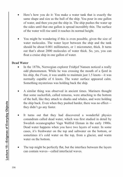
106

Lect

ure

15—

Enig

mas

of E

very

day

Obj

ects

• Here’s how you do it: You make a water tank that is exactly the same shape and size as the hull of the ship. You pour in one gallon of water, and then you put the ship in. The ship pushes the water up the sides until that one gallon is spread incredibly thin. The surface of the water will rise until it reaches its normal height.

• You might be wondering if this is even possible, given the size of water molecules. The water layer between the ship and the tank should be about 0.001 millimeters, or 1 micrometer, thick. It turns out that’s about 2000 molecules of water thick. So, yes, you can float a cruise ship in one gallon of water.

Dead Water • In the 1870s, Norwegian explorer Fridtjof Nansen noticed a really

odd phenomenon. While he was crossing the mouth of a fjord in his ship, the Fram, it was unable to maintain just 1.5 knots—it was normally capable of 6 knots. The water surface appeared calm. Something mysterious was holding back the ship.

• A similar thing was observed in ancient times. Mariners thought that some suckerfish, called remoras, were attaching to the bottom of the hull, like they attach to sharks and whales, and were holding the ship back. Even when they pushed harder, there was no effect—they didn’t go any faster.

• It turns out that they had discovered a wonderful physics conundrum called dead water, which was first studied in detail by Swedish oceanographer Vagn Walfrid Ekman in the early 1900s. Dead water happens when you have two layers of water. In some cases, it’s freshwater on the top and saltwater on the bottom, or sometimes it’s cold water on the top, from a glacier, and warm water on the bottom.

• The top might be perfectly flat, but the interface between the layers can contain waves—called interfacial waves.

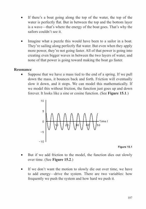
107

• If there’s a boat going along the top of the water, the top of the water is perfectly flat. But in between the top and the bottom layer is a wave—that’s where the energy of the boat goes. That’s why the sailors couldn’t see it.

• Imagine what a puzzle this would have been to a sailor in a boat. They’re sailing along perfectly flat water. But even when they apply more power, they’re not going faster. All of that power is going into creating even bigger waves in between the two layers of water, and none of that power is going toward making the boat go faster.

Resonance • Suppose that we have a mass tied to the end of a spring. If we pull

down the mass, it bounces back and forth. Friction will eventually slow it down, and it stops. We can model this mathematically. If we model this without friction, the function just goes up and down forever. It looks like a sine or cosine function. (See Figure 15.1.)

• But if we add friction to the model, the function dies out slowly over time. (See Figure 15.2.)

• If we don’t want the motion to slowly die out over time, we have to add energy—drive the system. There are two variables: how frequently we push the system and how hard we push it.

Figure 15.1

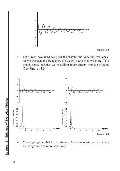
108

Lect

ure

15—

Enig

mas

of E

very

day

Obj

ects

• Let’s keep how hard we push it constant and vary the frequency. As we increase the frequency, the weight starts to move more. This makes sense because we’re adding more energy into the system. (See Figure 15.3.)

• You might guess that this continues. As we increase the frequency, the weight moves more and more.

Figure 15.2

Figure 15.3

109

• The theoretical model predicts something different—that if we increase the frequency too much, the motion is going to decrease.

• In reality, when the frequency is really high, the weight hardly moves at all. And only when we slow down—only when we get to a magical frequency—does the weight move a lot. If we go much slower, the weight hardly moves. Amazingly, putting more energy in doesn’t mean that the weight moves more.

• The curve shows a peak frequency. It’s a very narrow peak. If we miss this resonant frequency—if we go either too fast or too slow—we get much less vibration. Think about being on a swing. There is an exact right time to pump your legs when you’re on that swing. If you pump more frequently or less frequently, you’ll be completely off.

• This resonance phenomenon is important in a surprising variety of situations. Nearly everything has a particular frequency it “wants” to vibrate at. There are interesting musical applications. In your shower, there’s probably a particular note that sounds really loud when you sing it.

• If the vibration happens to be exactly at the resonant frequency, then instead of changing the frequency, you change the amplitude. If the amplitude is high enough, you get into trouble. For example, the opening of the Millennium Bridge in London was delayed because there was a side-to-side resonance that happened to be about the same as a walking pace.

• One astonishing fact of mathematics and music is that your ears are using resonance to break down sound waves into their component frequencies. The different parts of your cochlea resonate at different frequencies. When you hear a sound, your ear is breaking it down into those different frequencies.

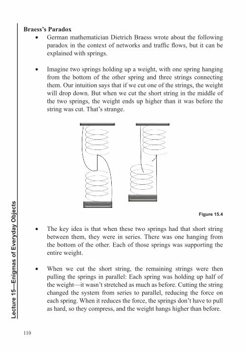
110

Lect

ure

15—

Enig

mas

of E

very

day

Obj

ects

Braess’s Paradox • German mathematician Dietrich Braess wrote about the following

paradox in the context of networks and traffic flows, but it can be explained with springs.

• Imagine two springs holding up a weight, with one spring hanging from the bottom of the other spring and three strings connecting them. Our intuition says that if we cut one of the strings, the weight will drop down. But when we cut the short string in the middle of the two springs, the weight ends up higher than it was before the string was cut. That’s strange.

• The key idea is that when these two springs had that short string between them, they were in series. There was one hanging from the bottom of the other. Each of those springs was supporting the entire weight.

• When we cut the short string, the remaining strings were then pulling the springs in parallel: Each spring was holding up half of the weight—it wasn’t stretched as much as before. Cutting the string changed the system from series to parallel, reducing the force on each spring. When it reduces the force, the springs don’t have to pull as hard, so they compress, and the weight hangs higher than before.

Figure 15.4

111

• By itself, this is just a strange oddity, a counterintuitive fact about springs. But the implications are just as unexpected, and there are important implications in terms of modern infrastructure. For example, this paradox, called Braess’s paradox, has implications in traffic flow.

• Imagine traffic between points A and B on a path that takes the shape of a figure 8, with A at the top and B at the bottom. If you’re traveling from A to B, you would have the following 3 options: You could follow all the roads down the left side of the map (route 1); you could start down the right side, take the short road across the middle, and then come down the left side (route 2); or you could stay down the right side entirely (route 3).

• If the path is an appropriate figure 8, route 2, where you cut across the middle, would be the shortest. And nearly everyone takes it because it’s the shortest, so you get significant traffic delays.

• Suppose that construction closed that short connector road. Then, commuters have 2 options: down the left side or the right side. The distance is about the same, so about half the commuters go each of these directions. The result is less congestion—no traffic jam.

A

1 2

3

B

Figure 15.5

112

Lect

ure

15—

Enig

mas

of E

very

day

Obj

ects

• That’s already weird: You close a road and make traffic flow better and improve average travel times. But imagine that the road hasn’t been built yet. Should the road be constructed? Without it, traffic was split between only 2 routes. But with the additional road, traffic will snarl to a stop.

• Building a new road sometimes makes traffic worse. The U.S. government spends more than $100 billion per year on roads. It’s probably important to know that building these roads won’t make traffic worse. People are paying taxes to build these roads, and if they’re making their commutes worse, that’s highly problematic.

• How likely is it that this will happen? In 1983, Willard Zangwill and Richard Steinberg answered this question—and the answer is surprising. If you randomly choose where to add a road, the chance of making traffic worse (Braess’s paradox) is about 50%.

Belmont, “NSF Fluid Mechanics Series: 18. Stratified Flow.”

MatthieuMercier’s channel, “Dead Water Phenomenon (‘toy box’).”

Pickover, Every Insanely Mystifying Paradox in Physics.

Roughgarden, Selfish Routing and the Price of Anarchy.

Veritasium, “Slinky Drop Answer.”

1. The traffic-flow version of Braess’s paradox includes a hint of the prisoner’s dilemma. How are they related?

2. Sometimes when driving on a dirt road, you come to a patch of “washboard” where the road has a regular set of ripples. Most people argue that you should slow down drastically to keep your car from shaking too much—but speeding up also works. Why?

Suggested Reading

Problems

113

Surprises of the Small and SpeedyLecture 16

In this lecture, you will learn about a few of the many paradoxes of modern physics. Specifically, you will learn about paradoxes of post-1905 physics: relativity and quantum mechanics. These types of paradoxes—

and modern physics in general—challenge our common sense. All of our life experiences are on the scale of the human body, so our common sense breaks down at high speeds, such as the speed of light, and with really small or really large objects. These paradoxes show how different the world is at very high speeds and small scales.

Einstein’s Theory of Relativity • In the late 1800s, physicists figured out that light doesn’t travel like

objects do at our scale. If a ball is thrown at you at 100 miles per hour, if you move away at 20 miles per hour, it appears to be going just 80 miles per hour relative to you.

• The Michelson-Morley experiment showed that light moves the same speed independent of the motion of the observer. Other experiments showed that fast particles don’t behave like Newton’s laws would suggest.

• Einstein’s basic idea was that light will always be observed at the speed of light—a constant (c), 186,000 miles per second, or about 3 ×108 meters per second. If you’re moving away from the light source, the light doesn’t appear to be going slower. It’s still that same speed. If you’re moving toward the light source, it doesn’t speed up. It’s still that same speed.

• The second part of Einstein’s idea was that the rules of physics are the same at any constant speed. If you’re traveling in a smooth train at a constant speed, if there are no windows, there’s no way to tell that you’re moving.

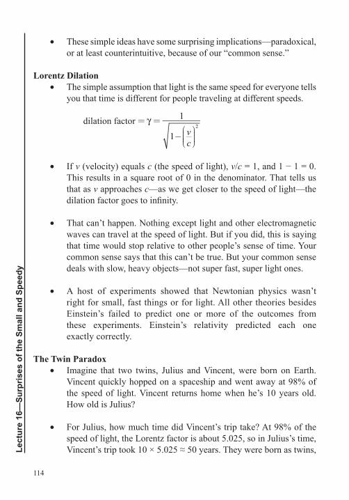
114

Lect

ure

16—

Surp

rises

of t

he S

mal

l and

Spe

edy

• These simple ideas have some surprising implications—paradoxical, or at least counterintuitive, because of our “common sense.”

Lorentz Dilation • The simple assumption that light is the same speed for everyone tells

you that time is different for people traveling at different speeds.

dilation factor = = 1

1 vc

2

• If v (velocity) equals c (the speed of light), v/c = 1, and 1 − 1 = 0. This results in a square root of 0 in the denominator. That tells us that as v approaches c—as we get closer to the speed of light—the dilation factor goes to infinity.

• That can’t happen. Nothing except light and other electromagnetic waves can travel at the speed of light. But if you did, this is saying that time would stop relative to other people’s sense of time. Your common sense says that this can’t be true. But your common sense deals with slow, heavy objects—not super fast, super light ones.

• A host of experiments showed that Newtonian physics wasn’t right for small, fast things or for light. All other theories besides Einstein’s failed to predict one or more of the outcomes from these experiments. Einstein’s relativity predicted each one exactly correctly.

The Twin Paradox • Imagine that two twins, Julius and Vincent, were born on Earth.

Vincent quickly hopped on a spaceship and went away at 98% of the speed of light. Vincent returns home when he’s 10 years old. How old is Julius?

• For Julius, how much time did Vincent’s trip take? At 98% of the speed of light, the Lorentz factor is about 5.025, so in Julius’s time, Vincent’s trip took 10 × 5.025 ≈ 50 years. They were born as twins,

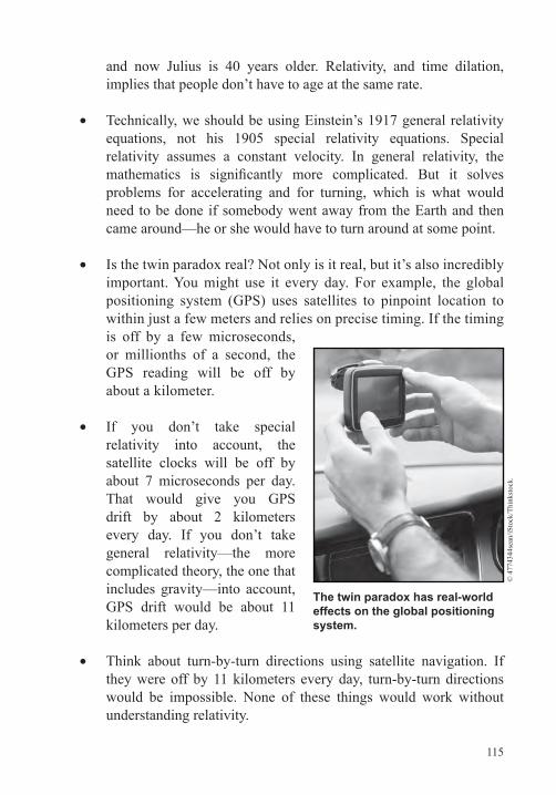
115

and now Julius is 40 years older. Relativity, and time dilation, implies that people don’t have to age at the same rate.

• Technically, we should be using Einstein’s 1917 general relativity equations, not his 1905 special relativity equations. Special relativity assumes a constant velocity. In general relativity, the mathematics is significantly more complicated. But it solves problems for accelerating and for turning, which is what would need to be done if somebody went away from the Earth and then came around—he or she would have to turn around at some point.

• Is the twin paradox real? Not only is it real, but it’s also incredibly important. You might use it every day. For example, the global positioning system (GPS) uses satellites to pinpoint location to within just a few meters and relies on precise timing. If the timing is off by a few microseconds, or millionths of a second, the GPS reading will be off by about a kilometer.

• If you don’t take special relativity into account, the satellite clocks will be off by about 7 microseconds per day. That would give you GPS drift by about 2 kilometers every day. If you don’t take general relativity—the more complicated theory, the one that includes gravity—into account, GPS drift would be about 11 kilometers per day.

• Think about turn-by-turn directions using satellite navigation. If they were off by 11 kilometers every day, turn-by-turn directions would be impossible. None of these things would work without understanding relativity.

The twin paradox has real-world effects on the global positioning system.

© 4

7743

44se

an/iS

tock

/Thi

nkst

ock.

116

Lect

ure

16—

Surp

rises

of t

he S

mal

l and

Spe

edy

• Once you understand relativity, you have to agree that twins might not age at the same rate. With regard to the twin paradox, as yet, no one has figured out a way to do it. We can’t travel that fast. But in theory, it’s exactly correct.

Quantum Mechanics • The physics field of quantum mechanics developed over the early

part of the 20th century with Albert Einstein, Werner Heisenberg, Max Born, Erwin Schrödinger, Wolfgang Pauli, David Hilbert, John von Neumann, and others. The fundamental discovery about atomic and subatomic particles was that small-scale objects and light have both wavelike and particle-like properties.

• On the human scale, particles—think about billiard balls—do one thing. Waves—think about water waves—behave differently. If a particle goes through a hole in a fence, it either makes it through or doesn’t. If a wave goes through a hole in a fence, it radiates out in a circular pattern.

• We think on our scale: Two particles interact—they either hit or don’t—and two waves interact—they interfere (with two boat wakes, sometimes you get really large waves and sometimes you get small ones). But atoms, electrons, and other subatomic particles sometimes behave like particles and sometimes like waves. This is a highly mathematical, very complicated theory.

The Double-Slit Experiment • The double-slit experiment is a classic mind-bending physics

experiment. If you shoot things—such as light, electrons, or something else—at a screen that has two slits, what comes through the other side onto a target?

• The prediction from our common sense is that the particles will go through one of the slits, if they go through at all, and hit one spot somewhere on the target. But if it were waves, the waves would go through both slits and create circular waves around those slits on the backside, and those would interfere with each other.

117

• If you do this experiment with hundreds of photons or electrons at a screen, each one hits the target at some specific place. But on the target, it’s not just two places that they end up; instead, they form a pattern that matches the interference pattern you would expect if they were two waves.

• The best mathematical description of this is that each electron is best described by a probability distribution (where it’s likely to be if you use a sensor to detect it). That distribution is a wave that goes through both slits—it creates its own interference.

• So, each electron is really a wave. That’s strange. In order to see the interference pattern, we detect each electron as hitting in a particular place, but with thousands of trials, we see a pattern emerge. It’s like waves interacting—the high spots and the low spots, not just in two places, one behind each slit.

• It gets more counterintuitive. If you put detectors at the slits, then each particle goes through just one of the slits. Each particle has its waveform, which tells you the probability of it being in different places. But when you detect the particle, the waveform collapses. It’s like its wavelike properties cease and its particle-like properties dominate.

• But before you detect the particle, where is it? Mathematics says that it’s everywhere the waveform says it is. The particle isn’t in a place; the wave is in many places.

• You shoot electrons, or photons, or neutrons at a double slit, and without detection, each one goes through both slits. This is truly counterintuitive. What is the behavior of these things? Are they particles? Are they waves? Are they both?

• It’s just very different at their scale—10−15 meters. Our intuition is based on objects at our scale. That intuition fails very badly at such a small scale.

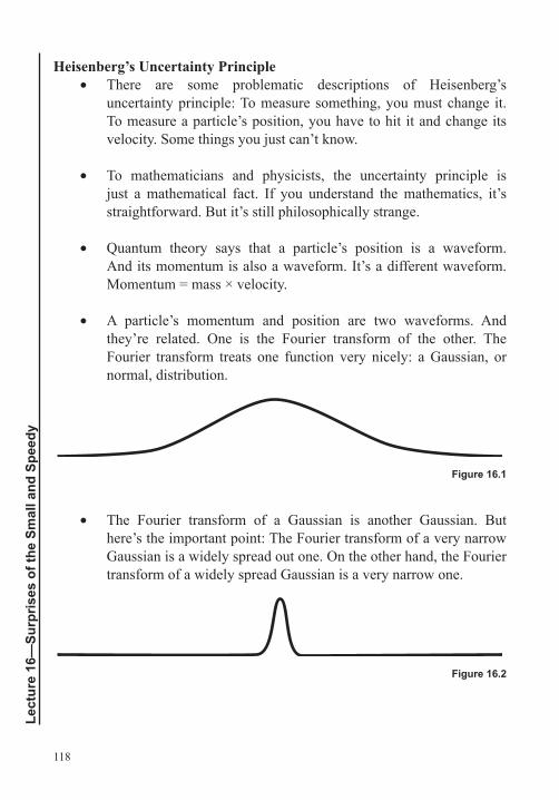
118

Lect

ure

16—

Surp

rises

of t

he S

mal

l and

Spe

edy

Heisenberg’s Uncertainty Principle • There are some problematic descriptions of Heisenberg’s

uncertainty principle: To measure something, you must change it. To measure a particle’s position, you have to hit it and change its velocity. Some things you just can’t know.

• To mathematicians and physicists, the uncertainty principle is just a mathematical fact. If you understand the mathematics, it’s straightforward. But it’s still philosophically strange.

• Quantum theory says that a particle’s position is a waveform. And its momentum is also a waveform. It’s a different waveform. Momentum = mass × velocity.

• A particle’s momentum and position are two waveforms. And they’re related. One is the Fourier transform of the other. The Fourier transform treats one function very nicely: a Gaussian, or normal, distribution.

• The Fourier transform of a Gaussian is another Gaussian. But here’s the important point: The Fourier transform of a very narrow Gaussian is a widely spread out one. On the other hand, the Fourier transform of a widely spread Gaussian is a very narrow one.

Figure 16.1

Figure 16.2

119

• A particle doesn’t have a position. The waveform tells you where you’re likely to find it if you detect it. A narrow Gaussian for position means that you know very well where the particle is. But that means that there’s a wide Gaussian for the momentum. The velocity is not very well pegged down.

• It goes the other way, too. If you have a very narrow Gaussian for momentum, that means that you know the velocity very accurately. Its Fourier transform will be a wide Gaussian for position. So, the location is not very well known.

• There’s an extreme case: If you know the position exactly, what happens? Mathematics says that the velocity might be anything. On the other hand, if you know the velocity exactly, the location might be anywhere. This is a simple mathematical relationship with a profound implication: Heisenberg’s uncertainty principle.

Al-Khalili, Paradox.

Gribbin, In Search of Schrodinger’s Cat.

Pickover, Every Insanely Mystifying Paradox in Physics.

1. One standard objection to the twin paradox states that in the frame of reference of each twin, the other moves away at a high speed. Thus, both would see the other as aging more slowly. What do Einstein’s theories have to say about this objection?

2. The EPR Paradox (named after Einstein, Podolsky, and Rosen) has received recent renewed attention, now described as quantum entanglement. Briefly, it states that if you could create two particles that were strongly correlated (for example, one spin up and the other spin down) and then separate the two by a long distance, then measuring the

Suggested Reading

Problems

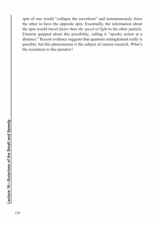
120

Lect

ure

16—

Surp

rises

of t

he S

mal

l and

Spe

edy

spin of one would “collapse the waveform” and instantaneously force the other to have the opposite spin. Essentially, the information about the spin would travel faster than the speed of light to the other particle. Einstein quipped about this possibility, calling it “spooky action at a distance.” Recent evidence suggests that quantum entanglement really is possible, but this phenomenon is the subject of current research. What’s the resolution to this paradox?

121

Bending Space and TimeLecture 17

In this lecture, you will try to solve some geometrical puzzles and paradoxes, including paradoxes that deal with squares, dots, circles, and globes. In the case of globe paradoxes, map distortions affect our view

of the world. Facts about the actual world surprise us, because we have internalized the distortions that are on the flat maps that we’re so used to. Grappling with these types of conundrums and exposing our naïve thinking leads us to be better thinkers and to have a clearer, more accurate view of the world.

Missing Square • The following puzzle, which is included in Sam Loyd’s Cyclopedia

of 5000 Puzzles, Tricks, and Conundrums, is a geometric mind bender about rearranging pieces, like tangrams.

• Four pieces are arranged in a perfect square. The square is 8 × 8, which equals 64 square units. We can rearrange the pieces into a rectangle that is 5 × 13, which equals 65 square units. How can the same pieces cover more area?

Figure 17.1

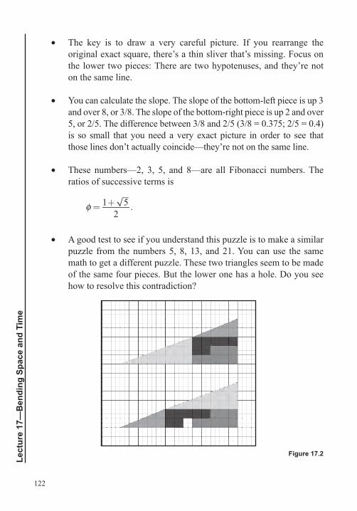
122

Lect

ure

17—

Ben

ding

Spa

ce a

nd T

ime

• The key is to draw a very careful picture. If you rearrange the original exact square, there’s a thin sliver that’s missing. Focus on the lower two pieces: There are two hypotenuses, and they’re not on the same line.

• You can calculate the slope. The slope of the bottom-left piece is up 3 and over 8, or 3/8. The slope of the bottom-right piece is up 2 and over 5, or 2/5. The difference between 3/8 and 2/5 (3/8 = 0.375; 2/5 = 0.4) is so small that you need a very exact picture in order to see that those lines don’t actually coincide—they’re not on the same line.

• These numbers—2, 3, 5, and 8—are all Fibonacci numbers. The ratios of successive terms is

φ= +1 52

.

• A good test to see if you understand this puzzle is to make a similar puzzle from the numbers 5, 8, 13, and 21. You can use the same math to get a different puzzle. These two triangles seem to be made of the same four pieces. But the lower one has a hole. Do you see how to resolve this contradiction?

Figure 17.2

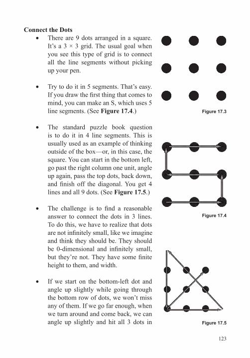
123

Connect the Dots • There are 9 dots arranged in a square.

It’s a 3 × 3 grid. The usual goal when you see this type of grid is to connect all the line segments without picking up your pen.

• Try to do it in 5 segments. That’s easy. If you draw the first thing that comes to mind, you can make an S, which uses 5 line segments. (See Figure 17.4.)

• The standard puzzle book question is to do it in 4 line segments. This is usually used as an example of thinking outside of the box—or, in this case, the square. You can start in the bottom left, go past the right column one unit, angle up again, pass the top dots, back down, and finish off the diagonal. You get 4 lines and all 9 dots. (See Figure 17.5.)

• The challenge is to find a reasonable answer to connect the dots in 3 lines. To do this, we have to realize that dots are not infinitely small, like we imagine and think they should be. They should be 0-dimensional and infinitely small, but they’re not. They have some finite height to them, and width.

• If we start on the bottom-left dot and angle up slightly while going through the bottom row of dots, we won’t miss any of them. If we go far enough, when we turn around and come back, we can angle up slightly and hit all 3 dots in

Figure 17.3

Figure 17.4

Figure 17.5

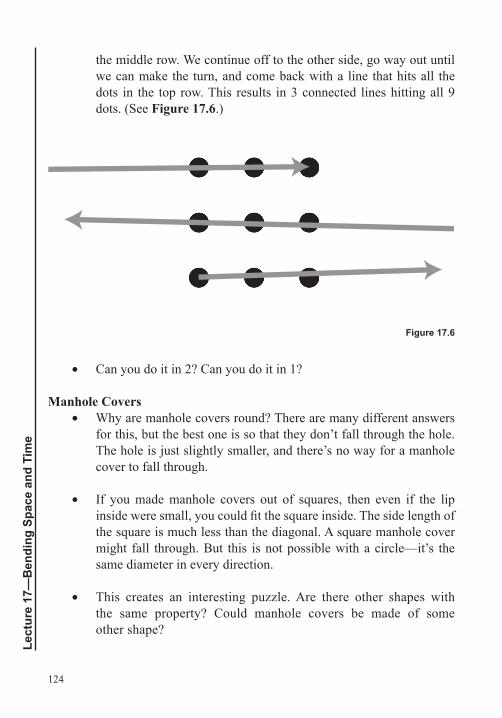
124

Lect

ure

17—

Ben

ding

Spa

ce a

nd T

ime

the middle row. We continue off to the other side, go way out until we can make the turn, and come back with a line that hits all the dots in the top row. This results in 3 connected lines hitting all 9 dots. (See Figure 17.6.)

• Can you do it in 2? Can you do it in 1?

Manhole Covers • Why are manhole covers round? There are many different answers

for this, but the best one is so that they don’t fall through the hole. The hole is just slightly smaller, and there’s no way for a manhole cover to fall through.

• If you made manhole covers out of squares, then even if the lip inside were small, you could fit the square inside. The side length of the square is much less than the diagonal. A square manhole cover might fall through. But this is not possible with a circle—it’s the same diameter in every direction.

• This creates an interesting puzzle. Are there other shapes with the same property? Could manhole covers be made of some other shape?

Figure 17.6

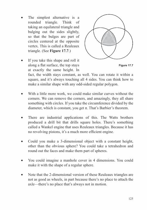
125

• The simplest alternative is a rounded triangle. Think of taking an equilateral triangle and bulging out the sides slightly, so that the bulges are part of circles centered at the opposite vertex. This is called a Reuleaux triangle. (See Figure 17.7.)

• If you take this shape and roll it along a flat surface, the top stays at exactly the same height. In fact, the width stays constant, as well. You can rotate it within a square, and it’s always touching all 4 sides. You can think how to make a similar shape with any odd-sided regular polygon.

• With a little more work, we could make similar curves without the corners. We can remove the corners, and amazingly, they all share something with circles. If you take the circumference divided by the diameter, which is constant, you get π. That’s Barbier’s theorem.

• There are industrial applications of this. The Watts brothers produced a drill bit that drills square holes. There’s something called a Wankel engine that uses Reuleaux triangles. Because it has no revolving pistons, it’s a much more efficient engine.

• Could you make a 3-dimensional object with a constant height, other than the obvious sphere? You could take a tetrahedron and round out the faces and make them part of spheres.

• You could imagine a manhole cover in 4 dimensions. You could make it with the shape of a regular sphere.

• Note that the 2-dimensional version of these Reuleaux triangles are not as good as wheels, in part because there’s no place to attach the axle—there’s no place that’s always not in motion.

Figure 17.7

126

Lect

ure

17—

Ben

ding

Spa

ce a

nd T

ime

Globe Paradoxes • A man gets up, walks 1 mile directly south, 1 mile directly east,

sees a bear, and then walks 1 mile directly north—back to where he started. What color was the bear?

• This question is a good reminder that we live on a (nearly) spherical planet, not on a flat plane—although our maps are flat. If you were on a plane and went 1 mile south, 1 mile east, and 1 mile north, you would end up 1 mile from where you started. But on a sphere, you’re at the North Pole. The north and south legs are not parallel on a globe. So, the answer to this riddle is that the bear must be white: a polar bear.

• But the North Pole is not the only answer. There is another place on Earth where you could walk 1 mile south, 1 mile east, 1 mile north, and get back to where you started. The key is not the north-south legs, but the east leg.

• Somewhere around the South Pole, there is a circle where the perimeter of that circle is exactly 1 mile. If you use that as your east leg, that leg ends exactly where it started. Then, the north and south legs would be exactly on the same ground.

• That circle is about 1/(2π) away from the South Pole. The circumference would be 2πr. And if r is 1/(2π), then the two π‘s cancel, and you get 1 mile. It’s not exactly 1/(2π) because of the curvature of the Earth.

• Note that anywhere that’s 1 mile north of that circle will do, so any point about 1 + 1/(2π) north of the South Pole.

• In fact, you could find even more places. We found a circle so that 1 mile east went around once. The key insight here is that with an even smaller circle, 1 mile east could go around twice—or, with an even smaller circle, three or four times. If that 1 mile wraps around exactly k times, then the north and south parts will be exactly matched up. And that is a problem generally.

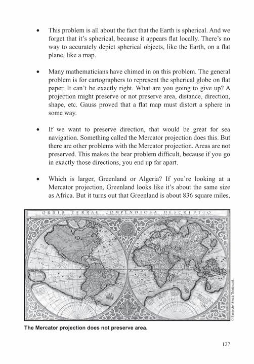
127

• This problem is all about the fact that the Earth is spherical. And we forget that it’s spherical, because it appears flat locally. There’s no way to accurately depict spherical objects, like the Earth, on a flat plane, like a map.

• Many mathematicians have chimed in on this problem. The general problem is for cartographers to represent the spherical globe on flat paper. It can’t be exactly right. What are you going to give up? A projection might preserve or not preserve area, distance, direction, shape, etc. Gauss proved that a flat map must distort a sphere in some way.

• If we want to preserve direction, that would be great for sea navigation. Something called the Mercator projection does this. But there are other problems with the Mercator projection. Areas are not preserved. This makes the bear problem difficult, because if you go in exactly those directions, you end up far apart.

• Which is larger, Greenland or Algeria? If you’re looking at a Mercator projection, Greenland looks like it’s about the same size as Africa. But it turns out that Greenland is about 836 square miles,

The Mercator projection does not preserve area.

© P

astic

cio/

iSto

ck/T

hink

stoc

k.

128

Lect

ure

17—

Ben

ding

Spa

ce a

nd T

ime

and Algeria is 919,000 square miles, so Algeria is bigger. The Mercator map is well known to distort the world, but it’s still used today in many places.

• If you want to preserve areas—to avoid the Mercator problem—there are other projections that will work, such as the Gall-Peters projection and the Lambert projection. In all of these, Greenland is not quite so big. But there are other problems. Distances and directions are distorted.

• There are many problems with rectangular maps. Nearby points end up very far apart. For example, on many maps, northern Canada and northern Russia look like they’re far away, but they’re actually very close if you go over the North Pole.

• There are sinusoidal projections that fix this. And, in fact, some of them have equal area. Vertical and horizontal scales are correct everywhere, but it seriously distorts the world in other ways. For example, in some of these maps, the poles look like they’re pointed, but they’re not. The Mollweide projection avoids the points at the poles, but it’s bad for navigation.

• For all of these maps, north is up—for no good mathematical reason. Somehow, the United States and Europe are central. All of these projections are interesting mathematically.

Gardner, Hexaflexagons and Other Mathematical Diversions.

———, Wheels, Life, and Other Mathematical Amusements.

Suggested Reading

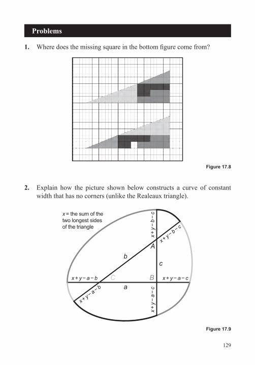
129

1. Where does the missing square in the bottom figure come from?

2. Explain how the picture shown below constructs a curve of constant width that has no corners (unlike the Realeaux triangle).

Problems

Figure 17.8

c

aC B

Ab

x + y

− b

− c

x + y −

b − c

x + y − a − c

x + y

− a

− c

x + y − a − b

x + y −

a − b

x = the sum of the two longest sides of the triangle

Figure 17.9

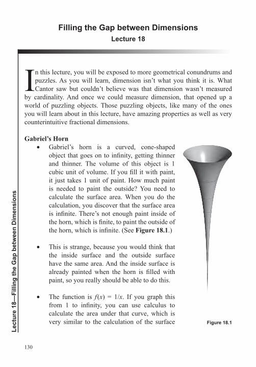
130

Lect

ure

18—

Filli

ng th

e G

ap b

etw

een

Dim

ensi

ons

Filling the Gap between DimensionsLecture 18

In this lecture, you will be exposed to more geometrical conundrums and puzzles. As you will learn, dimension isn’t what you think it is. What Cantor saw but couldn’t believe was that dimension wasn’t measured

by cardinality. And once we could measure dimension, that opened up a world of puzzling objects. Those puzzling objects, like many of the ones you will learn about in this lecture, have amazing properties as well as very counterintuitive fractional dimensions.

Gabriel’s Horn • Gabriel’s horn is a curved, cone-shaped

object that goes on to infinity, getting thinner and thinner. The volume of this object is 1 cubic unit of volume. If you fill it with paint, it just takes 1 unit of paint. How much paint is needed to paint the outside? You need to calculate the surface area. When you do the calculation, you discover that the surface area is infinite. There’s not enough paint inside of the horn, which is finite, to paint the outside of the horn, which is infinite. (See Figure 18.1.)

• This is strange, because you would think that the inside surface and the outside surface have the same area. And the inside surface is already painted when the horn is filled with paint, so you really should be able to do this.

• The function is f (x) = 1/x. If you graph this from 1 to infinity, you can use calculus to calculate the area under that curve, which is very similar to the calculation of the surface Figure 18.1

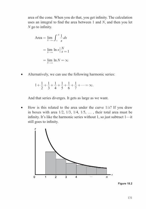
131

area of the cone. When you do that, you get infinity. The calculation uses an integral to find the area between 1 and N, and then you let N go to infinity.

∞

∞

∞

∫=

= =

= =∞

→

→

→

xdx

x Nx

N

Area lim 1

lim ln 1

lim ln

N

N

N

N

1

• Alternatively, we can use the following harmonic series:

�+ + + + + + + =∞1 12

13

14

15

16

17

.

And that series diverges. It gets as large as we want.

• How is this related to the area under the curve 1/x? If you draw in boxes with area 1/2, 1/3, 1/4, 1/5, … , their total area must be infinity. It’s like the harmonic series without 1, so just subtract 1—it still goes to infinity.

Figure 18.2

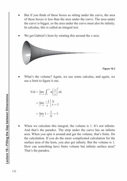
132

Lect

ure

18—

Filli

ng th

e G

ap b

etw

een

Dim

ensi

ons

• But if you think of these boxes as sitting under the curve, the area of these boxes is less than the area under the curve. The area under the curve is bigger, so the area under the curve must also be infinity. In calculus, this is called an integral test.

• We get Gabriel’s horn by rotating this around the x-axis.

• What’s the volume? Again, we use some calculus, and again, we use a limit to figure it out.

Vol= limN

1x

2

dx1

N

= limN

1x

Nx=1

= limN

1 1N=1.

π

• When we calculate this integral, the volume is 1. It’s not infinite. And that’s the paradox. The strip under the curve has an infinite area. When you spin it around and get the volume, that’s finite. Do the calculation. If you do the more complicated calculation for the surface area of the horn, you also get infinity. But the volume is 1. How can something have finite volume but infinite surface area? That’s the paradox.

Figure 18.3

133

• Italian mathematician Evangelista Torricelli discovered this in the 1600s without calculus. It’s sometimes called Torricelli’s trumpet. Torricelli thought that this horn, or trumpet, was really paradoxical. Tip it up and fill it with just a can of paint, but that’s not enough to paint itself?

• Area and length are different dimensions, different measurements. The same is true of area and volume. Area is 2-dimensional, and volume is 3-dimensional. This explains Gabriel’s horn. The volume is finite, but the surface area is infinite. There’s no contradiction; those are just measuring very different things.

• In fact, in some sense, every can of paint is like this, at least in theory. It definitely has a finite volume. There’s no problem with that. In reality, a layer of paint is a finite (nonzero) thickness. It’s at least a molecule of paint thick. So, its surface area, which is just a mathematical idea, is zero thickness. In theory, any positive volume of paint covers any infinite surface, because they’re just different measurements, different dimensions. In reality, paint molecules create a limit. Eventually, the paint molecules would get caught in Gabriel’s horn.

Fractals • In 1904, Swedish mathematician Niels Fabian Helge von Koch

discovered a curve with finite area but infinite length. Later, we would call these fractals. We start with an equilateral triangle. On each edge, we find the middle third. On the outside of that middle third, we build an equilateral triangle, and then remove the middle third.

• You can think about those steps as a single action: You take any line segment and replace its middle third with the remaining two edges of a triangle. You can do this action to all of the edges, and then you can do it again on all of the smaller edges, and so on. The end result of infinitely many of these actions is called the Koch snowflake. (See Figure 18.4.)

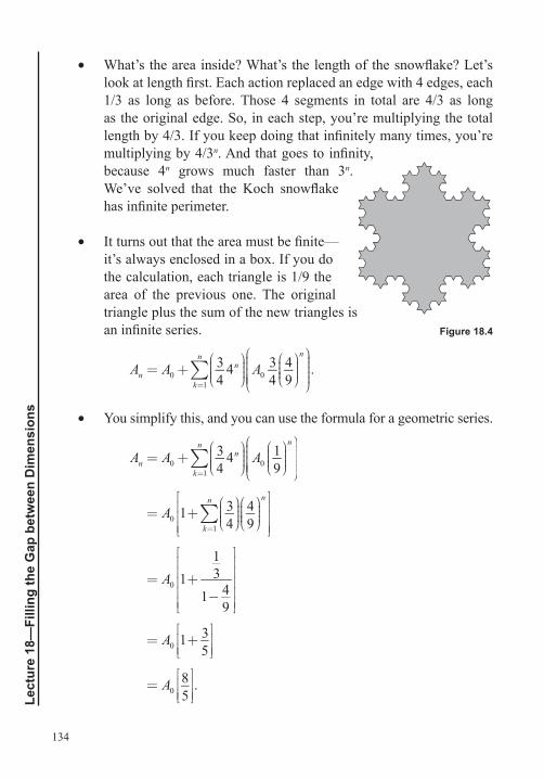
134

Lect

ure

18—

Filli

ng th

e G

ap b

etw

een

Dim

ensi

ons

• What’s the area inside? What’s the length of the snowflake? Let’s look at length first. Each action replaced an edge with 4 edges, each 1/3 as long as before. Those 4 segments in total are 4/3 as long as the original edge. So, in each step, you’re multiplying the total length by 4/3. If you keep doing that infinitely many times, you’re multiplying by 4/3n. And that goes to infinity, because 4n grows much faster than 3n. We’ve solved that the Koch snowflake has infinite perimeter.

• It turns out that the area must be finite—it’s always enclosed in a box. If you do the calculation, each triangle is 1/9 the area of the previous one. The original triangle plus the sum of the new triangles is an infinite series.

An = A0+344n

k=1

n

A03449

n

.

• You simplify this, and you can use the formula for a geometric series.

An = A0+344n

k=1

n

A019

n

= A0 1+3449

n

k=1

n

= A0 1+13

1 49

= A0 1+35

= A085.

Figure 18.4

135

• The area of the Koch snowflake is the area of the original triangle times 8/5. The entire figure is just 60% more than the original, but the perimeter is infinite. It has a finite area, but the perimeter is infinite. There’s no contradiction here. The area and perimeter are just different; they’re two different attributes of a figure.

The Cantor Set • The Koch snowflake is an example of “actual infinity”—the end

result of an infinite process. There are similar ideas with other geometrical figures. For example, you could take the unit interval 0 to 1, which is an uncountable set. There’s no correspondence with the natural numbers.

• In the first step, we remove the middle third of the line segment from 1/3 to 2/3. (We don’t remove the endpoints, 1/3 and 2/3, but everything in between them.) We’re left with 2 line segments, and we can remove the middle thirds of those. Then, we’re left with 4 line segments, and we remove the middle thirds of those, and so on, infinitely many times.

• What’s left? In 1875, Oxford math professor H. J. S. Smith first discovered sets like this. He studied their strange properties. But nobody noticed Smith’s revolutionary work. It was a few years later, in 1884, when Georg Cantor published similar work. Now we call the set the Cantor set.

• There are many strange things about the Cantor set. One of these is the dimension. What’s the dimension of the Cantor set? You’d think it might be 1-dimensional. It starts out as a line segment. But there are no intervals left. Every time you add an interval, you remove the middle third. So, maybe it’s 0-dimensional. Maybe it’s just points.

• The answer is that the dimension of the Cantor set is log3(2), which is about 0.63-dimensional. This is a non-integer dimension.

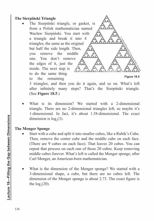
136

Lect

ure

18—

Filli

ng th

e G

ap b

etw

een

Dim

ensi

ons

The Sierpiński Triangle • The Sierpiński triangle, or gasket, is

from a Polish mathematician named Wacław Sierpiński. You start with a triangle and break it into 4 triangles, the same as the original but half the side length. Then, you remove the middle one. You don’t remove the edges of it, just the inside. The next step is to do the same thing to the remaining 3 triangles, and then you do it again, and so on. What’s left after infinitely many steps? That’s the Sierpiński triangle. (See Figure 18.5.)

• What is its dimension? We started with a 2-dimensional triangle. There are no 2-dimensional triangles left, so maybe it’s 1-dimensional. In fact, it’s about 1.58-dimensional. The exact dimension is log2(3).

The Menger Sponge • Start with a cube and split it into smaller cubes, like a Rubik’s Cube.

Then, remove the center cube and the middle cube on each face. (There are 9 cubes on each face). That leaves 20 cubes. You can repeat that process on each one of those 20 cubes. Keep removing middle cubes forever. What’s left is called the Menger sponge, after Carl Menger, an American-born mathematician.

• What is the dimension of the Menger sponge? We started with a 3-dimensional shape, a cube, but there are no cubes left. The dimension of the Menger sponge is about 2.73. The exact figure is the log3(20).

Figure 18.5

© Solkoll/W

ikimedia Com

mons/Public Dom

ain.

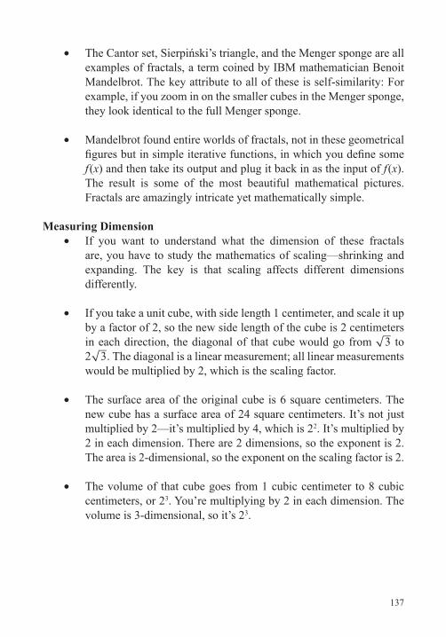
137

• The Cantor set, Sierpiński’s triangle, and the Menger sponge are all examples of fractals, a term coined by IBM mathematician Benoit Mandelbrot. The key attribute to all of these is self-similarity: For example, if you zoom in on the smaller cubes in the Menger sponge, they look identical to the full Menger sponge.

• Mandelbrot found entire worlds of fractals, not in these geometrical figures but in simple iterative functions, in which you define some f (x) and then take its output and plug it back in as the input of f (x). The result is some of the most beautiful mathematical pictures. Fractals are amazingly intricate yet mathematically simple.

Measuring Dimension • If you want to understand what the dimension of these fractals

are, you have to study the mathematics of scaling—shrinking and expanding. The key is that scaling affects different dimensions differently.

• If you take a unit cube, with side length 1 centimeter, and scale it up by a factor of 2, so the new side length of the cube is 2 centimeters in each direction, the diagonal of that cube would go from 3 to 2 3. The diagonal is a linear measurement; all linear measurements would be multiplied by 2, which is the scaling factor.

• The surface area of the original cube is 6 square centimeters. The new cube has a surface area of 24 square centimeters. It’s not just multiplied by 2—it’s multiplied by 4, which is 22. It’s multiplied by 2 in each dimension. There are 2 dimensions, so the exponent is 2. The area is 2-dimensional, so the exponent on the scaling factor is 2.

• The volume of that cube goes from 1 cubic centimeter to 8 cubic centimeters, or 23. You’re multiplying by 2 in each dimension. The volume is 3-dimensional, so it’s 23.

138

Lect

ure

18—

Filli

ng th

e G

ap b

etw

een

Dim

ensi

ons

• How something scales depends on its dimension. If you scale by a factor of 3, anything linear (lengths) will scale by a factor of 3. Anything 2-dimensional (areas) will scale by a factor of 32. Anything 3-dimensional (volume) will scale by a factor of 33, or 27. The dimension shows up as the exponent on the scaling factor.

Mandelbrot, The Fractal Geometry of Nature.

1. What’s the dimension of this Sierpiński carpet?

2. How could computer graphic artists use fractal principles in their work?

Suggested Reading

Problems

Figure 18.6

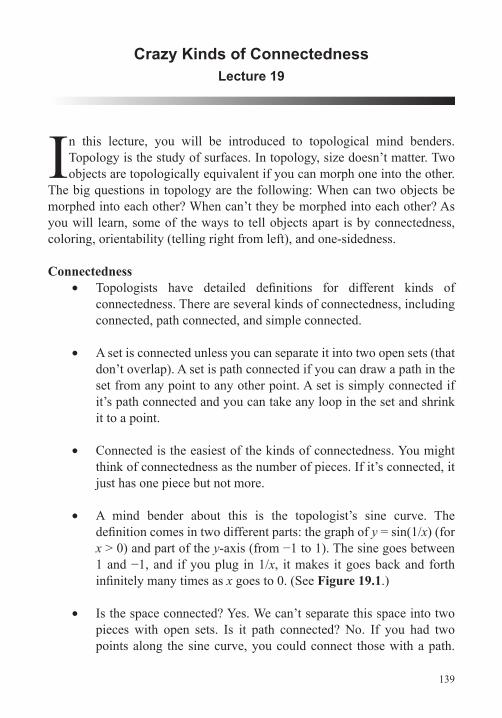
139

Crazy Kinds of ConnectednessLecture 19

In this lecture, you will be introduced to topological mind benders. Topology is the study of surfaces. In topology, size doesn’t matter. Two objects are topologically equivalent if you can morph one into the other.

The big questions in topology are the following: When can two objects be morphed into each other? When can’t they be morphed into each other? As you will learn, some of the ways to tell objects apart is by connectedness, coloring, orientability (telling right from left), and one-sidedness.

Connectedness • Topologists have detailed definitions for different kinds of

connectedness. There are several kinds of connectedness, including connected, path connected, and simple connected.

• A set is connected unless you can separate it into two open sets (that don’t overlap). A set is path connected if you can draw a path in the set from any point to any other point. A set is simply connected if it’s path connected and you can take any loop in the set and shrink it to a point.

• Connected is the easiest of the kinds of connectedness. You might think of connectedness as the number of pieces. If it’s connected, it just has one piece but not more.

• A mind bender about this is the topologist’s sine curve. The definition comes in two different parts: the graph of y = sin(1/x) (for x > 0) and part of the y-axis (from −1 to 1). The sine goes between 1 and −1, and if you plug in 1/x, it makes it goes back and forth infinitely many times as x goes to 0. (See Figure 19.1.)

• Is the space connected? Yes. We can’t separate this space into two pieces with open sets. Is it path connected? No. If you had two points along the sine curve, you could connect those with a path.

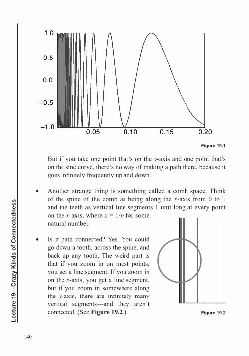
140

Lect

ure

19—

Cra

zy K

inds

of C

onne

cted

ness

But if you take one point that’s on the y-axis and one point that’s on the sine curve, there’s no way of making a path there, because it goes infinitely frequently up and down.

• Another strange thing is something called a comb space. Think of the spine of the comb as being along the x-axis from 0 to 1 and the teeth as vertical line segments 1 unit long at every point on the x-axis, where x = 1/n for some natural number.

• Is it path connected? Yes. You could go down a tooth, across the spine, and back up any tooth. The weird part is that if you zoom in on most points, you get a line segment. If you zoom in on the x-axis, you get a line segment, but if you zoom in somewhere along the y-axis, there are infinitely many vertical segments—and they aren’t connected. (See Figure 19.2.)

Figure 19.1

Figure 19.2

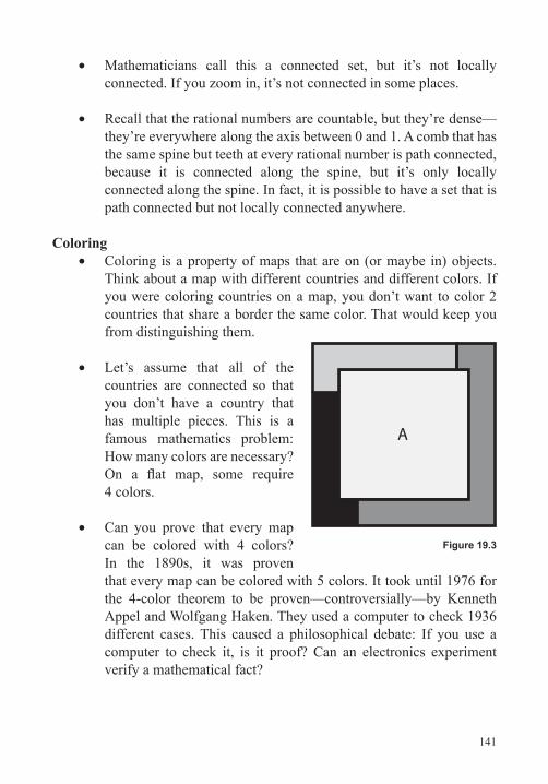
141

• Mathematicians call this a connected set, but it’s not locally connected. If you zoom in, it’s not connected in some places.

• Recall that the rational numbers are countable, but they’re dense—they’re everywhere along the axis between 0 and 1. A comb that has the same spine but teeth at every rational number is path connected, because it is connected along the spine, but it’s only locally connected along the spine. In fact, it is possible to have a set that is path connected but not locally connected anywhere.

Coloring • Coloring is a property of maps that are on (or maybe in) objects.

Think about a map with different countries and different colors. If you were coloring countries on a map, you don’t want to color 2 countries that share a border the same color. That would keep you from distinguishing them.

• Let’s assume that all of the countries are connected so that you don’t have a country that has multiple pieces. This is a famous mathematics problem: How many colors are necessary? On a flat map, some require 4 colors.

• Can you prove that every map can be colored with 4 colors? In the 1890s, it was proven that every map can be colored with 5 colors. It took until 1976 for the 4-color theorem to be proven—controversially—by Kenneth Appel and Wolfgang Haken. They used a computer to check 1936 different cases. This caused a philosophical debate: If you use a computer to check it, is it proof? Can an electronics experiment verify a mathematical fact?

A

Figure 19.3

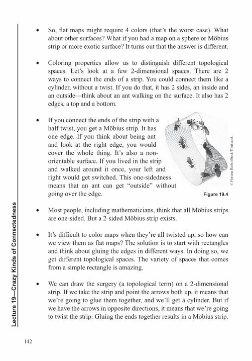
142

Lect

ure

19—

Cra

zy K

inds

of C

onne

cted

ness

• So, flat maps might require 4 colors (that’s the worst case). What about other surfaces? What if you had a map on a sphere or Möbius strip or more exotic surface? It turns out that the answer is different.

• Coloring properties allow us to distinguish different topological spaces. Let’s look at a few 2-dimensional spaces. There are 2 ways to connect the ends of a strip. You could connect them like a cylinder, without a twist. If you do that, it has 2 sides, an inside and an outside—think about an ant walking on the surface. It also has 2 edges, a top and a bottom.

• If you connect the ends of the strip with a half twist, you get a Möbius strip. It has one edge. If you think about being ant and look at the right edge, you would cover the whole thing. It’s also a non-orientable surface. If you lived in the strip and walked around it once, your left and right would get switched. This one-sidedness means that an ant can get “outside” without going over the edge.

• Most people, including mathematicians, think that all Möbius strips are one-sided. But a 2-sided Möbius strip exists.

• It’s difficult to color maps when they’re all twisted up, so how can we view them as flat maps? The solution is to start with rectangles and think about gluing the edges in different ways. In doing so, we get different topological spaces. The variety of spaces that comes from a simple rectangle is amazing.

• We can draw the surgery (a topological term) on a 2-dimensional strip. If we take the strip and point the arrows both up, it means that we’re going to glue them together, and we’ll get a cylinder. But if we have the arrows in opposite directions, it means that we’re going to twist the strip. Gluing the ends together results in a Möbius strip.

Figure 19.4

© F

loria

na B

arbu

/iSto

ck/T

hink

stoc

k.

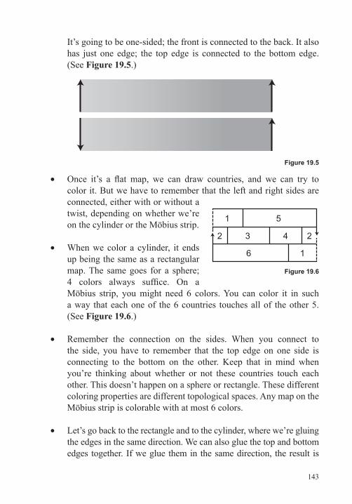
143

It’s going to be one-sided; the front is connected to the back. It also has just one edge; the top edge is connected to the bottom edge. (See Figure 19.5.)

• Once it’s a flat map, we can draw countries, and we can try to color it. But we have to remember that the left and right sides are connected, either with or without a twist, depending on whether we’re on the cylinder or the Möbius strip.

• When we color a cylinder, it ends up being the same as a rectangular map. The same goes for a sphere; 4 colors always suffice. On a Möbius strip, you might need 6 colors. You can color it in such a way that each one of the 6 countries touches all of the other 5. (See Figure 19.6.)

• Remember the connection on the sides. When you connect to the side, you have to remember that the top edge on one side is connecting to the bottom on the other. Keep that in mind when you’re thinking about whether or not these countries touch each other. This doesn’t happen on a sphere or rectangle. These different coloring properties are different topological spaces. Any map on the Möbius strip is colorable with at most 6 colors.

• Let’s go back to the rectangle and to the cylinder, where we’re gluing the edges in the same direction. We can also glue the top and bottom edges together. If we glue them in the same direction, the result is

Figure 19.5

1

2

6 1

3 4 2

5

Figure 19.6

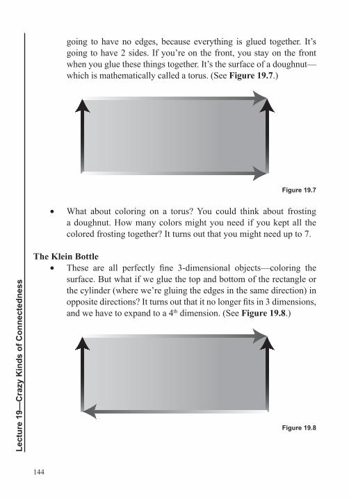
144

Lect

ure

19—

Cra

zy K

inds

of C

onne

cted

ness

going to have no edges, because everything is glued together. It’s going to have 2 sides. If you’re on the front, you stay on the front when you glue these things together. It’s the surface of a doughnut—which is mathematically called a torus. (See Figure 19.7.)

• What about coloring on a torus? You could think about frosting a doughnut. How many colors might you need if you kept all the colored frosting together? It turns out that you might need up to 7.

The Klein Bottle • These are all perfectly fine 3-dimensional objects—coloring the

surface. But what if we glue the top and bottom of the rectangle or the cylinder (where we’re gluing the edges in the same direction) in opposite directions? It turns out that it no longer fits in 3 dimensions, and we have to expand to a 4th dimension. (See Figure 19.8.)

Figure 19.7

Figure 19.8

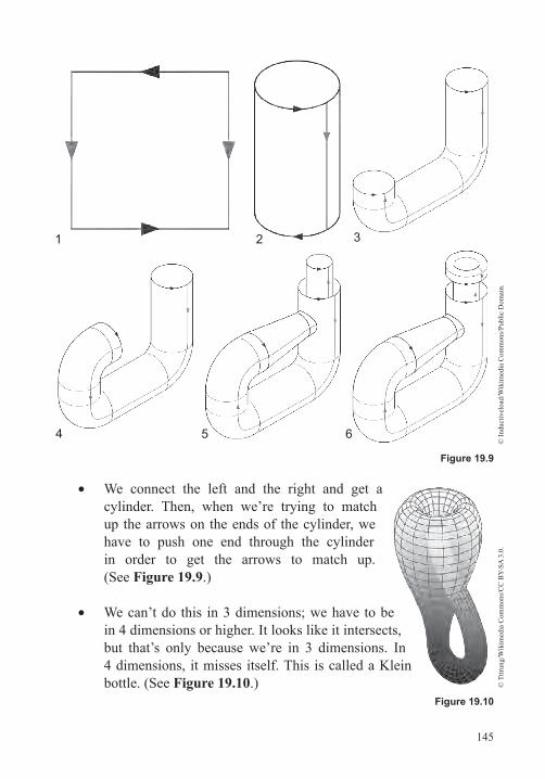
145

• We connect the left and the right and get a cylinder. Then, when we’re trying to match up the arrows on the ends of the cylinder, we have to push one end through the cylinder in order to get the arrows to match up. (See Figure 19.9.)

• We can’t do this in 3 dimensions; we have to be in 4 dimensions or higher. It looks like it intersects, but that’s only because we’re in 3 dimensions. In 4 dimensions, it misses itself. This is called a Klein bottle. (See Figure 19.10.)

Figure 19.9

1 3

5

2

4 6

Figure 19.10

© T

ttrun

g/W

ikim

edia

Com

mon

s/C

C B

Y-SA

3.0

.©

Indu

ctiv

eloa

d/W

ikim

edia

Com

mon

s/Pu

blic

Dom

ain.

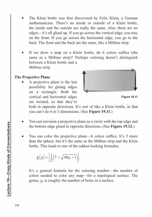
146

Lect

ure

19—

Cra

zy K

inds

of C

onne

cted

ness

• The Klein bottle was first discovered by Felix Klein, a German mathematician. There’s no inside or outside of a Klein bottle; the inside and the outside are really the same. Also, there are no edges—it’s all glued up. If you go across the vertical edge, you stay on the front. If you go across the horizontal edge, you go to the back. The front and the back are the same, like a Möbius strip.

• If we drew a map on a Klein bottle, do 6 colors suffice (the same as a Möbius strip)? Perhaps coloring doesn’t distinguish between a Klein bottle and a Möbius strip.

The Projective Plane • A projective plane is the last

possibility for gluing edges on a rectangle. Both the vertical and horizontal edges are twisted, so that they’re both in opposite directions. It’s sort of like a Klein bottle, in that you can’t do it in 3 dimensions. (See Figure 19.11.)

• You can envision a projective plane as a circle with the top edge and the bottom edge glued in opposite directions. (See Figure 19.12.)

• You can color the projective plane—6 colors suffice. It’s 2 more than the sphere, but it’s the same as the Möbius strip and the Klein bottle. This leads to one of the oddest-looking formulas:

g( )= 127+ 48g+1( ) .

It’s a general formula for the coloring number—the number of colors needed to color any map—for a topological surface. The genus, g, is roughly the number of holes in a surface.

Figure 19.11

147

Weeks, The Shape of Space.

1. What would happen if you cut a Möbius strip in 3? (That is, make 2 cuts, 1/3 and 2/3 of the way across the strip, and continue along until the cuts met.) How many pieces would be created? Would the pieces be able to come apart, or would they be linked?

2. How do we make sense of the Klein bottle seemingly living in 3-dimensional space but somehow requiring a 4th dimension in order to “connect”?

Suggested Reading

Problems

The Projective Plane

Figure 19.12

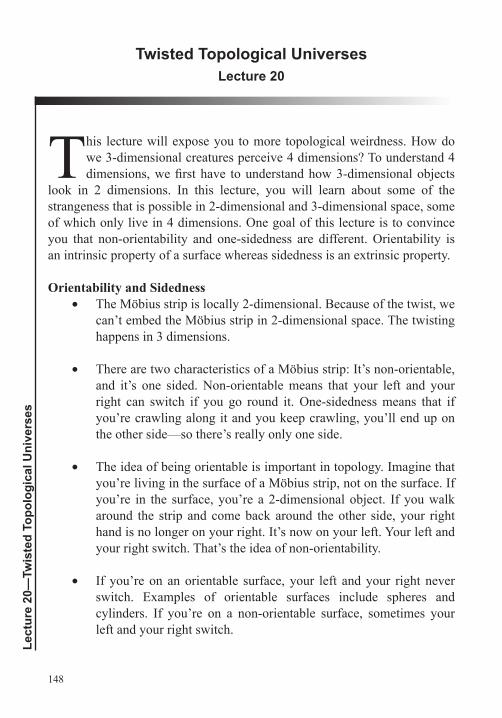
148

Lect

ure

20—

Twis

ted

Topo

logi

cal U

nive

rses

Twisted Topological UniversesLecture 20

This lecture will expose you to more topological weirdness. How do we 3-dimensional creatures perceive 4 dimensions? To understand 4 dimensions, we first have to understand how 3-dimensional objects

look in 2 dimensions. In this lecture, you will learn about some of the strangeness that is possible in 2-dimensional and 3-dimensional space, some of which only live in 4 dimensions. One goal of this lecture is to convince you that non-orientability and one-sidedness are different. Orientability is an intrinsic property of a surface whereas sidedness is an extrinsic property.

Orientability and Sidedness • The Möbius strip is locally 2-dimensional. Because of the twist, we

can’t embed the Möbius strip in 2-dimensional space. The twisting happens in 3 dimensions.

• There are two characteristics of a Möbius strip: It’s non-orientable, and it’s one sided. Non-orientable means that your left and your right can switch if you go round it. One-sidedness means that if you’re crawling along it and you keep crawling, you’ll end up on the other side—so there’s really only one side.

• The idea of being orientable is important in topology. Imagine that you’re living in the surface of a Möbius strip, not on the surface. If you’re in the surface, you’re a 2-dimensional object. If you walk around the strip and come back around the other side, your right hand is no longer on your right. It’s now on your left. Your left and your right switch. That’s the idea of non-orientability.

• If you’re on an orientable surface, your left and your right never switch. Examples of orientable surfaces include spheres and cylinders. If you’re on a non-orientable surface, sometimes your left and your right switch.

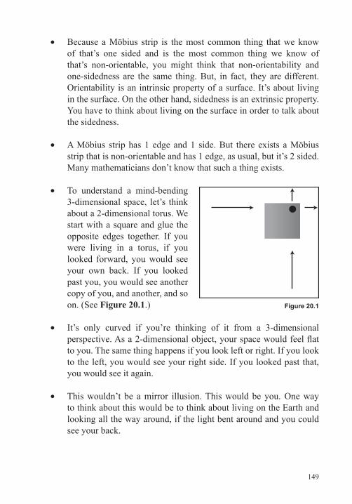
149

• Because a Möbius strip is the most common thing that we know of that’s one sided and is the most common thing we know of that’s non-orientable, you might think that non-orientability and one-sidedness are the same thing. But, in fact, they are different. Orientability is an intrinsic property of a surface. It’s about living in the surface. On the other hand, sidedness is an extrinsic property. You have to think about living on the surface in order to talk about the sidedness.

• A Möbius strip has 1 edge and 1 side. But there exists a Möbius strip that is non-orientable and has 1 edge, as usual, but it’s 2 sided. Many mathematicians don’t know that such a thing exists.

• To understand a mind-bending 3-dimensional space, let’s think about a 2-dimensional torus. We start with a square and glue the opposite edges together. If you were living in a torus, if you looked forward, you would see your own back. If you looked past you, you would see another copy of you, and another, and so on. (See Figure 20.1.)

• It’s only curved if you’re thinking of it from a 3-dimensional perspective. As a 2-dimensional object, your space would feel flat to you. The same thing happens if you look left or right. If you look to the left, you would see your right side. If you looked past that, you would see it again.

• This wouldn’t be a mirror illusion. This would be you. One way to think about this would be to think about living on the Earth and looking all the way around, if the light bent around and you could see your back.

Figure 20.1

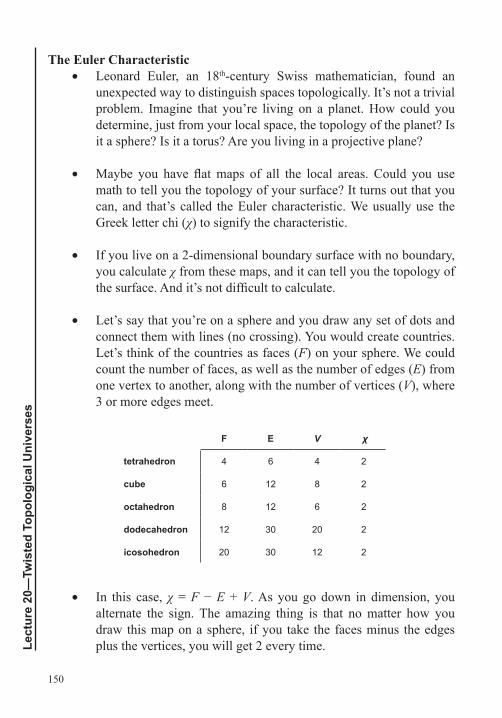
150

Lect

ure

20—

Twis

ted

Topo

logi

cal U

nive

rses

The Euler Characteristic • Leonard Euler, an 18th-century Swiss mathematician, found an

unexpected way to distinguish spaces topologically. It’s not a trivial problem. Imagine that you’re living on a planet. How could you determine, just from your local space, the topology of the planet? Is it a sphere? Is it a torus? Are you living in a projective plane?

• Maybe you have flat maps of all the local areas. Could you use math to tell you the topology of your surface? It turns out that you can, and that’s called the Euler characteristic. We usually use the Greek letter chi (χ) to signify the characteristic.

• If you live on a 2-dimensional boundary surface with no boundary, you calculate χ from these maps, and it can tell you the topology of the surface. And it’s not difficult to calculate.

• Let’s say that you’re on a sphere and you draw any set of dots and connect them with lines (no crossing). You would create countries. Let’s think of the countries as faces (F) on your sphere. We could count the number of faces, as well as the number of edges (E) from one vertex to another, along with the number of vertices (V), where 3 or more edges meet.

• In this case, χ = F − E + V. As you go down in dimension, you alternate the sign. The amazing thing is that no matter how you draw this map on a sphere, if you take the faces minus the edges plus the vertices, you will get 2 every time.

F E V χ

tetrahedron 4 6 4 2

cube 6 12 8 2

octahedron 8 12 6 2

dodecahedron 12 30 20 2

icosohedron 20 30 12 2

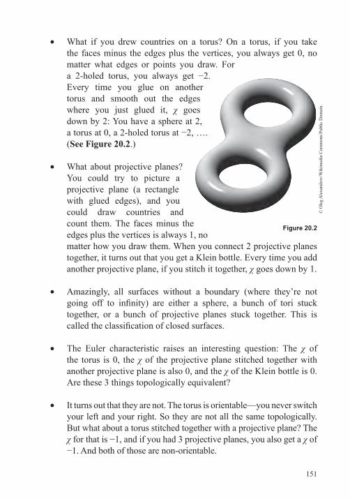
151

• What if you drew countries on a torus? On a torus, if you take the faces minus the edges plus the vertices, you always get 0, no matter what edges or points you draw. For a 2-holed torus, you always get −2. Every time you glue on another torus and smooth out the edges where you just glued it, χ goes down by 2: You have a sphere at 2, a torus at 0, a 2-holed torus at −2, …. (See Figure 20.2.)

• What about projective planes? You could try to picture a projective plane (a rectangle with glued edges), and you could draw countries and count them. The faces minus the edges plus the vertices is always 1, no matter how you draw them. When you connect 2 projective planes together, it turns out that you get a Klein bottle. Every time you add another projective plane, if you stitch it together, χ goes down by 1.

• Amazingly, all surfaces without a boundary (where they’re not going off to infinity) are either a sphere, a bunch of tori stuck together, or a bunch of projective planes stuck together. This is called the classification of closed surfaces.

• The Euler characteristic raises an interesting question: The χ of the torus is 0, the χ of the projective plane stitched together with another projective plane is also 0, and the χ of the Klein bottle is 0. Are these 3 things topologically equivalent?

• It turns out that they are not. The torus is orientable—you never switch your left and your right. So they are not all the same topologically. But what about a torus stitched together with a projective plane? The χ for that is −1, and if you had 3 projective planes, you also get a χ of −1. And both of those are non-orientable.

© O

leg

Ale

xand

rov/

Wik

imed

ia C

omm

ons/

Publ

ic D

omai

n.

Figure 20.2

152

Lect

ure

20—

Twis

ted

Topo

logi

cal U

nive

rses

• Are they topologically equivalent? It turns out that they are. It’s difficult to picture this. If you know the orientability and the Euler characteristic (information from a map), you can figure out what surface you’re on.

Geometry and Topology • Geometry seems rigid and fixed. Scaling matters, and the size of

things matters. We measure things in geometry. Topology is loose and rubbery. Morphing doesn’t matter. But, amazingly, they’re connected in deep ways.

• Many proofs of the Euler characteristic—which is something from topology—use very advanced mathematics. But we can use geometry to prove it. On a unit sphere, all countries are, for example, triangles. Let’s assume that all countries are triangles and all edges are straight. The goal is to prove that the faces minus the edges plus the vertices is equal to 2 (F − E + V = 2) on any sphere.

• Eventually, using geometry, we get to the Gauss-Bonnet theorem:

χκ π∫ =dA 2 .

• Kappa (κ) is a measurement of the curvature: κ = 0 for a flat space, κ > 0 for a spherical space, and κ < 0 for a hyperbolic space. In general, the Gauss-Bonnet theorem adds up the curvature over the entire surface (using an integral). When you add up the curvature over the entire surface, the result is 2πχ, which is the Euler characteristic.

• That’s amazing. The left side of the equation—the integral of κ over the entire area—is a measure of how curved the surface is, added up. The right side of the equation is 2πχ, the Euler characteristic, which is vertices minus edges plus faces. It doesn’t matter what the map is, what the countries are, or what borders you draw in.

153

• In other words, the left side is geometrical, where scale matters—we’re measuring curvature and adding it up. The right side is entirely topological: If you bend and twist and stretch a surface, it won’t change the topological properties. But it definitely changes the curvature, or the geometry.

• According to this formula, it doesn’t change the sum of the curvature over the entire surface. Somehow, the topological information (the number of holes or orientability) is encoded not in the curvature at any one point, but in the sum of the curvatures over the entire surface.

Weeks, The Shape of Space.

1. In the lecture, video tricks helped us “walk through” three different 3-manifolds: the 3-torus, a non-orientable 3-manifold (with the left and right walks glued with a half-twist), and a quarter-turn manifold. In what ways were those demonstrations not accurate depictions of what those spaces would look like?

Suggested Reading

Problem

154

Lect

ure

21—

Mor

e w

ith L

ess,

Som

ethi

ng fo

r Not

hing

More with Less, Something for NothingLecture 21

In this lecture, you will be exposed to geometrical optimization—or doing the most with the least. How should a grocer stack oranges to use the least space? How much room do you need in order to turn around a

needle? Sôichi Kakeya posed this problem in 1917. A decade later, Abram Besicovitch provided the shocking answer: Given any positive area, you can find a region of that area inside which your needle can turn around. He went a step further, showing that if you are just looking for a set that contains a line segment pointing in every direction, a measure 0 set can be found.

Isoperimetric Problems • Let’s say that you have a fixed length of string. How can you make

the biggest rectangle? You don’t want it to be long and skinny; instead, you want it to be square. You can either use algebra or calculus to verify that a square gives you the biggest area for a fixed perimeter of rectangle.

• What’s the biggest area (any shape) for a fixed length of string? It’s more difficult now. There are more possibilities. But it’s been known since the Greeks that the answer is a circle. Interestingly, a proof of this didn’t happen until the 1800s, when Jakob Steiner and others finished it.

• Suppose that you’re camping near a river and you see a campfire that’s getting out of hand in the distance. You have a bucket, but your bucket is empty. You know that you should run to the river with the bucket, get the water, and then run to the fire and put it out. What’s the shortest path? Where along the river should you go to get the water?

• There’s an easy way to solve this, as well as a difficult way that involves calculus. If you use calculus, you might say that x is the distance from the point on the water closest to you (but far from

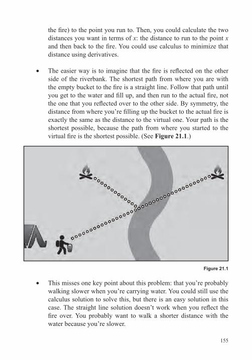
155

the fire) to the point you run to. Then, you could calculate the two distances you want in terms of x: the distance to run to the point x and then back to the fire. You could use calculus to minimize that distance using derivatives.

• The easier way is to imagine that the fire is reflected on the other side of the riverbank. The shortest path from where you are with the empty bucket to the fire is a straight line. Follow that path until you get to the water and fill up, and then run to the actual fire, not the one that you reflected over to the other side. By symmetry, the distance from where you’re filling up the bucket to the actual fire is exactly the same as the distance to the virtual one. Your path is the shortest possible, because the path from where you started to the virtual fire is the shortest possible. (See Figure 21.1.)

• This misses one key point about this problem: that you’re probably walking slower when you’re carrying water. You could still use the calculus solution to solve this, but there is an easy solution in this case. The straight line solution doesn’t work when you reflect the fire over. You probably want to walk a shorter distance with the water because you’re slower.

Figure 21.1

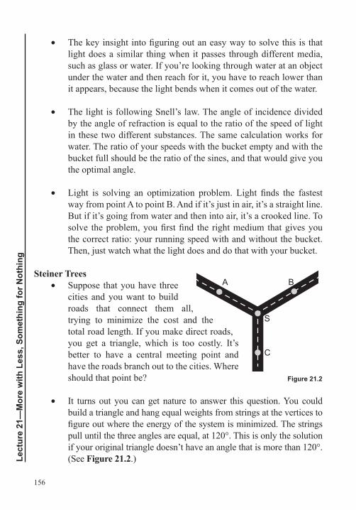
156

Lect

ure

21—

Mor

e w

ith L

ess,

Som

ethi

ng fo

r Not

hing

• The key insight into figuring out an easy way to solve this is that light does a similar thing when it passes through different media, such as glass or water. If you’re looking through water at an object under the water and then reach for it, you have to reach lower than it appears, because the light bends when it comes out of the water.

• The light is following Snell’s law. The angle of incidence divided by the angle of refraction is equal to the ratio of the speed of light in these two different substances. The same calculation works for water. The ratio of your speeds with the bucket empty and with the bucket full should be the ratio of the sines, and that would give you the optimal angle.

• Light is solving an optimization problem. Light finds the fastest way from point A to point B. And if it’s just in air, it’s a straight line. But if it’s going from water and then into air, it’s a crooked line. To solve the problem, you first find the right medium that gives you the correct ratio: your running speed with and without the bucket. Then, just watch what the light does and do that with your bucket.

Steiner Trees • Suppose that you have three

cities and you want to build roads that connect them all, trying to minimize the cost and the total road length. If you make direct roads, you get a triangle, which is too costly. It’s better to have a central meeting point and have the roads branch out to the cities. Where should that point be?

• It turns out you can get nature to answer this question. You could build a triangle and hang equal weights from strings at the vertices to figure out where the energy of the system is minimized. The strings pull until the three angles are equal, at 120°. This is only the solution if your original triangle doesn’t have an angle that is more than 120°. (See Figure 21.2.)

A B

C

S

Figure 21.2

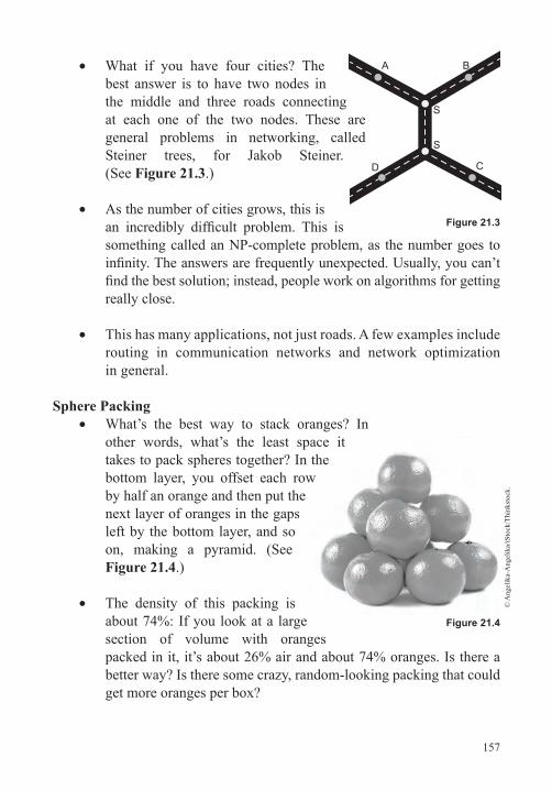
157

• What if you have four cities? The best answer is to have two nodes in the middle and three roads connecting at each one of the two nodes. These are general problems in networking, called Steiner trees, for Jakob Steiner. (See Figure 21.3.)

• As the number of cities grows, this is an incredibly difficult problem. This is something called an NP-complete problem, as the number goes to infinity. The answers are frequently unexpected. Usually, you can’t find the best solution; instead, people work on algorithms for getting really close.

• This has many applications, not just roads. A few examples include routing in communication networks and network optimization in general.

Sphere Packing • What’s the best way to stack oranges? In

other words, what’s the least space it takes to pack spheres together? In the bottom layer, you offset each row by half an orange and then put the next layer of oranges in the gaps left by the bottom layer, and so on, making a pyramid. (See Figure 21.4.)

• The density of this packing is about 74%: If you look at a large section of volume with oranges packed in it, it’s about 26% air and about 74% oranges. Is there a better way? Is there some crazy, random-looking packing that could get more oranges per box?

A B

C

S

D

S

Figure 21.3

Figure 21.4

© A

ngel

ika-

Ang

elik

a/iS

tock

/Thi

nkst

ock.

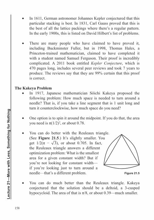
158

Lect

ure

21—

Mor

e w

ith L

ess,

Som

ethi

ng fo

r Not

hing

• In 1611, German astronomer Johannes Kepler conjectured that this particular stacking is best. In 1831, Carl Gauss proved that this is the best of all the lattice packings where there’s a regular pattern. In the early 1900s, this is listed on David Hilbert’s list of problems.

• There are many people who have claimed to have proved it, including Buckminster Fuller, but in 1998, Thomas Hales, a Princeton-trained mathematician, claimed to have completed it with a student named Samuel Ferguson. Their proof is incredibly complicated. A 2011 book entitled Kepler Conjecture, which is 470 pages long, includes several peer reviews and took 7 years to produce. The reviews say that they are 99% certain that this proof is correct.

The Kakeya Problem • In 1917, Japanese mathematician Sôichi Kakeya proposed the

following problem: How much space is needed to turn around a needle? That is, if you take a line segment that is 1 unit long and turn it counterclockwise, how much space do you need?

• One option is to spin it around the midpoint. If you do that, the area you need is π(1/2)2, or about 0.78.

• You can do better with the Reuleaux triangle. (See Figure 21.5.) It’s slightly smaller. You get 1/2(π − 3), or about 0.705. In fact, the Reuleaux triangle answers a different optimization problem: What is the smallest area for a given constant width? But if you’re not looking for constant width—if you’re looking just to turn around a needle—that’s a different problem.

• You can do much better than the Reuleaux triangle. Kakeya conjectured that the solution should be a deltoid, a 3-cusped hypocycloid. The area of that is π/8, or about 0.39—much smaller.

Figure 21.5

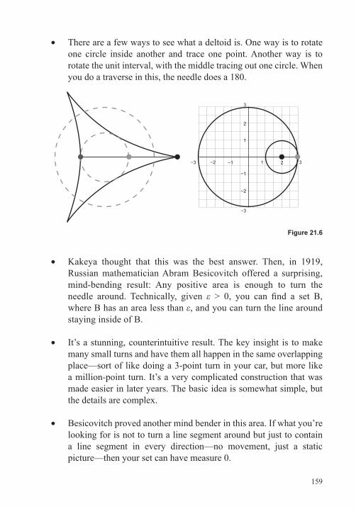
159

• There are a few ways to see what a deltoid is. One way is to rotate one circle inside another and trace one point. Another way is to rotate the unit interval, with the middle tracing out one circle. When you do a traverse in this, the needle does a 180.

• Kakeya thought that this was the best answer. Then, in 1919, Russian mathematician Abram Besicovitch offered a surprising, mind-bending result: Any positive area is enough to turn the needle around. Technically, given ε > 0, you can find a set B, where B has an area less than ε, and you can turn the line around staying inside of B.

• It’s a stunning, counterintuitive result. The key insight is to make many small turns and have them all happen in the same overlapping place—sort of like doing a 3-point turn in your car, but more like a million-point turn. It’s a very complicated construction that was made easier in later years. The basic idea is somewhat simple, but the details are complex.

• Besicovitch proved another mind bender in this area. If what you’re looking for is not to turn a line segment around but just to contain a line segment in every direction—no movement, just a static picture—then your set can have measure 0.

1

1

−1

−1

−2

−2

−3

−3

2

2

3

3

Figure 21.6

160

Lect

ure

21—

Mor

e w

ith L

ess,

Som

ethi

ng fo

r Not

hing

1. How could you alter the Cantor set construction so that the result doesn’t have measure 0?

2. In constructing a non-measurable set, we used the axiom of choice (to choose one point of each color—one point from each of the different rotations of the rational numbers). Could we construct such a set without using the axiom of choice?

Problems

161

When Measurement Is ImpossibleLecture 22

What can be measured, and what can’t be measured? In mathematics, sets of numbers should be easy to measure. In general, the length of the interval from a to b, as long as b is bigger than a, should

be b − a. Measuring complicated sets like the Cantor set should be trickier, but it should be doable. However, it turns out the measure of the Cantor set is 0. In this lecture, you will learn that we can’t measure all sets. You will discover why mathematicians wanted to measure sets in the first place, and then you will learn about constructing an unmeasurable set.

The Calculus of Measurement • A big part of calculus is about area. Mathematicians think of it as

physical area, but scientists and engineers think of it as measurement more generally. If the graph is velocity versus time, then the area is the net distance traveled. If the graph is pressure versus height, then the area measures force. If the graph is force versus distance, then the area measures work.

• To calculate area—to measure area—in calculus, you split things up into thin vertical boxes, and then you make an overestimate and an underestimate on each box (the biggest the function is and the smallest the function is in each one of those intervals). You add up the areas of the rectangles, and you get some number. Then, you do this again with thinner and thinner boxes, and you get a better and better approximation.

• If this works, then as the number of boxes goes to infinity—as their width goes to 0—the overestimates and the underestimates approach each other. That’s the area. You’ve measured what you want. We call them Riemann sums, and they are used throughout nearly all the sciences.

162

Lect

ure

22—

Whe

n M

easu

rem

ent I

s Im

poss

ible

• What if the process fails? What if the over- and underestimates don’t get close? Some strange functions could make this area process fail. Take f(x) = 1 if x is rational, and 0 if x isn’t. This is called Dirichlet’s function after the German mathematician Peter Dirichlet.

• What is the area under f between x = 0 and x = 1? If we try Riemann’s method, we split 0 to 1 up into small intervals. On any interval, the overestimate—the biggest the function is on any of those intervals—is always 1. There are always rational numbers there. The underestimate is always going to be 0, because there are always irrational numbers there. If you add up the results, the overestimate over the entire interval will always be exactly 1, and the underestimate will be exactly 0. The width of this interval is 1.

• You never get any closer no matter how many boxes you take. What do we do about this? The answer was in Henri Lebesgue’s 1902 dissertation. The big idea is to take horizontal boxes instead of taking vertical boxes.

• Vertical boxes give us Riemann integration, and the key is the maximum and minimum of the function on each interval. Horizontal boxes give us Lebesgue integration, and the key is the size of the set of points where f is bigger than some constant level.

• What is the measure of a set of points where f is less than or equal to a constant? With Dirichlet’s function, f = 1 on the rational numbers, and f = 0 on the irrational numbers. The height on the rational numbers is 1, so the area under that should be 1 times the measure of the rational numbers. (See Figure 22.1.)

• What should the measure of the rational numbers be? (This is different from the cardinality of the rational numbers.) You might guess the answer from probability: 0% of the numbers are rational, so the measure should be 0. Remember, we’re using the interval length.

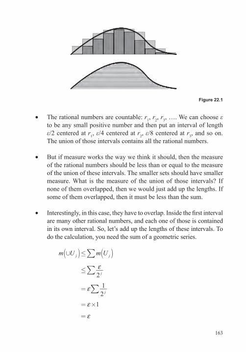
163

• The rational numbers are countable: r1, r2, r3, …. We can choose ε to be any small positive number and then put an interval of length ε/2 centered at r1, ε/4 centered at r2, ε/8 centered at r3, and so on. The union of those intervals contains all the rational numbers.

• But if measure works the way we think it should, then the measure of the rational numbers should be less than or equal to the measure of the union of these intervals. The smaller sets should have smaller measure. What is the measure of the union of those intervals? If none of them overlapped, then we would just add up the lengths. If some of them overlapped, then it must be less than the sum.

• Interestingly, in this case, they have to overlap. Inside the first interval are many other rational numbers, and each one of those is contained in its own interval. So, let’s add up the lengths of these intervals. To do the calculation, you need the sum of a geometric series.

ε

ε

ε

ε

∑

∑

∑

( ) ( )∪ ≤

≤

=

= ×

=

m U m U

2121

j j

j

j

Figure 22.1

164

Lect

ure

22—

Whe

n M

easu

rem

ent I

s Im

poss

ible

• The end result is that the length of the rational numbers is less than ε. That is true for any ε, so the measure of the rational numbers must be 0.

• Note that it’s really important that the length of these intervals is decreasing. If the length of the intervals were staying the same, if you add up infinitely many small positive numbers, you get infinity.

• What’s weird about this is that the rational numbers are everywhere—they are dense—but they have measure 0. With Dirichlet’s function, Riemann integration fails, but Lebesgue integration succeeds.

The Measure of the Cantor Set • Maybe “measure 0” is the same as “countable.” The measures are

countable, and the rational numbers have measure 0. In fact, so far, the countable sets are the same as the sets that have measure 0, and the uncountable sets have positive length.

• The Cantor set is uncountable, but it has length 0. If we return to the Cantor set, where we take the set [0, 1] and remove the middle thirds, there are no intervals left. Every time we take an interval, we split it further. It’s not connected; it’s split into small pieces. In fact, we call it totally disconnected. Sometimes people refer to it as Cantor dust. The natural numbers and the integers are also totally disconnected.

• But you might think that the Cantor set is just the endpoints. We remove the open middle thirds. We don’t remove 1/3 and 2/3, so maybe it’s the endpoints: 1/3, 2/3, 1/9, 2/9, 7/9, 8/9, …. If it were, it would be countable because we just listed them. You could match them up in a 1-to-1 correspondence with the natural numbers.

• So, is the Cantor set countable like the natural numbers and the integers? No, it turns out that it’s uncountable. It can’t fit into Hotel Infinity. It turns out that the Cantor set is perfectly matched, in a 1-to-1 manner, with the interval from 0 to 1. The integral from 0 to 1 is uncountable; therefore, the Cantor set is uncountable.

165

• The measure is surprisingly easy—it’s 0. It’s an uncountable set that has measure 0. It’s not even 1-dimensional. It has a fractional dimension between 0 and 1. That means that it has to have length 0.

• For the total length at each stage, we’re removing the middle third, so 2/3 remains. Then, the next time, we’re removing 1/3 of what was left. At each stage, 2/3 of what was left before remains. So, we’re really just multiplying the previous total length by 2/3. If we do n steps, we would multiply by (2/3)n. And (2/3)n goes to 0 as n goes to infinity. The 3n of the denominator grows much faster than the 2n in the numerator. The Cantor set is inside each one of those sets that goes to 0. The Cantor set must have measure 0.

Not Every Set Is Measurable • Suppose that we could measure everything. What are good

attributes of measurement? Each set gets a number, or size. ○ First, that number should be nonnegative.

○ Second, it should be additive. If you take two sets, a and b, and they are disjoint, if we put them together, the measure of the union should be the same as if we measured them separately—the measure of a plus the measure of b.

○ Third, any real sense of measurement should not be affected by rigid motion. If you rotate a set, or translate it from one place to another, it should have the same measure.

○ Finally, it should work for intervals: The measure of the length of the interval from a to b should just be the length, or b − a.

• The surprising result is that these attributes tell us that some sets are not measurable. You cannot measure everything.

• The result of the proof should seem familiar; no system does everything you want. The goal is to construct a set that must have positive measure—but it can’t have positive measure. What we conclude from that is that it’s not measurable.

166

Lect

ure

22—

Whe

n M

easu

rem

ent I

s Im

poss

ible

1. If you alter the construction of the Cantor set, starting with the open interval (0,1) and at each stage removing the closed middle third, is the resulting set countable or uncountable?

2. In constructing a non-measurable Vitali set, why is it so important that the rotations of the rational numbers are all disjoint? (That is, if two rotations don’t produce the same set, then they are disjoint.) In other words, where in the argument do we use the fact that these sets partition the circle?

Problems

167

Banach-Tarski’s 1 = 1 + 1Lecture 23

Mathematicians are in nearly universal agreement that the strangest paradox in mathematics is the Banach-Tarski paradox. As you will learn in this lecture, this paradox involves creating 2 balls

from 1—splitting 1 ball into a finite number of pieces and rearranging the pieces to get 2 balls of the same size. Interestingly, only a minority of mathematicians has ever seen the proof of this theorem. Rarely discussed, also, are the implications, or corollaries, of this theorem, including that you can take a pea-sized ball, split it up into a finite (very large) number of pieces, and reassemble the pieces—move and rotate them—to get a ball the size of the Sun.

The Banach-Tarski Paradox • Imagine all possible words using finitely many letters—finitely

many copies of a and b. Like Arabic, these strings of letters are read from the right to the left. A word might be just a, or just b, or ba, or ab, or even abbbaaabbaa. If you do a cardinality check, you discover that there are countably many words.

• Eventually, it’s not just going to be the letters a and b: a is going to be a 120° rotation around one axis. If you do that 3 times, you get a 360° rotation, which is the same as doing nothing. In other words, aaa is the same as doing nothing.

• On the other hand, b is going to be a 180° rotation around a different axis. If you do that rotation 2 times, bb, that’s going to be a 360° rotation, which is the same as doing nothing.

• Because of this, anytime we have 3 a’s in a row or 2 b’s in row, we’re going to remove them. It’s similar to simplifying a fraction. We can also write a2 for aa. Then, every word alternates b’s with either a or a2.

168

Lect

ure

23—

Ban

ach-

Tars

ki’s

1 =

1 +

1

• We’re going to put all of these words into a set, called G. We combine words by appending one to the other, called concatenation.

• For example, if we were to take aba2 and concatenate with a2ba, we just push them together and then simplify: aba2 × a2ba = aba4ba = ababa (because a3, which equals aaa, can be removed).

• Every word has an anti-word. The word aba has the anti-word a2ba2. They annihilate each other: If you concatenate them, you get a3 in the middle, and that can be removed. Then, you get b2 in the middle, and that can be removed. Finally, you get a3, which can be removed. Everything disappears: a2ba2 × aba = a2ba2aba = a2b2a = a3 = 1. We’ll call that the unit.

• Each word is a complicated sequence of rotations, and the anti-word is the process for undoing that sequence of rotations. In the technical language of mathematics, this is a “group,” like the integers with addition, except we have a particular set of words with concatenation. And the anti-words are the inverses. This particular group is called a free group on 2 elements, modulo a3 and b2.

• Decomposing G, the group of words, with a’s and b’s, where a3 = b2 = 1, is the heart of Banach-Tarski. It was proved in 1914 by German mathematician Felix Hausdorff.

• He also applied this to when a and b are rotations of a sphere, where a is a rotation around the north pole of 120°, 1/3 of the way around, so that a3 is the identity, and b is a rotation around some other axis of 180°. So, you do a 3 times, and you get back to where you start; you do b 2 times, and you get back to where you start.

• It’s important to choose the axis for the b rotation. We want to make sure that the angle between the north pole and the b axis doesn’t divide 360° in any rational number. We do this to make sure that no simplified word gets back to 1.

169

• Every word we have—for example, aba2ba—is a sequence of rotations. If you have a sequence of rotations, when you rotate and then rotate and then rotate, it’s equivalent to a single rotation.

• The rest of the proof of Banach-Tarski follows very closely with the construction of nonmeasurable sets. It involves thinking of different sets as “colored,” where the number of different colors is uncountable. It also involves creating a new set, S, which contains one point of each color.

• Then, the rotations, or words, in G act on S. The splitting of G creates subsets of the sphere, and then the paradox of G becomes the paradox of the sphere. Once we have the paradox on the sphere, which is just the outer shell, those sets can be extended inward to get a paradox on the entire sphere. That’s Banach-Tarski.

• The group, G, is split into 6 pieces, and we can rearrange those to get two copies of G. We can take 3 pieces and reassemble them to make an entire sphere and take the other 3 pieces and reassemble them to make the entire sphere again. We rearrange the 6 pieces by applying a and b in the correct way to get two entire copies of G.

• We use G to split the sphere into 6 pieces. The 6 pieces are rearranged by applying a and b, which are just rotations of the sphere. We rearrange those 6 pieces to get two entire copies of the sphere.

• The key fact is that when we apply any word in G to S, it never overlaps with S. When we apply all of G to S, we get the entire sphere. The splitting that we have of G into 6 pieces allows us to get a splitting of the entire sphere into 6 pieces when we apply those pieces to the set S.

• When we apply just parts of G to S, we get pieces that behave just as strangely as they did when we were thinking of them as just words in G.

170

Lect

ure

23—

Ban

ach-

Tars

ki’s

1 =

1 +

1

• The really paradoxical part is done. To get from the shell of the sphere to the ball, we have to extend these points inward toward 0. Then, we can create 2 balls out of 1.

Complications and Corollaries • There are 2 complications that require technical fixes. One is that

every rotation fixes 2 points—the ends of the axis of rotation, or poles—and those points are problems. Luckily, G is a countable set, and each word in G fixes to each of these points, so it’s a countable number of problems where we have this.

• The second problem is the center of the sphere. We extend things in from the shell toward the center, but we don’t say what to do at the very center of the sphere. The center is not in any set.

• These problems are countable. One set is countable, where you rotate the fixed points, and the other is just a single point. But, together, they make up a countable set. Stefan Banach and Alfred Tarski found a complicated and ingenious fix for this.

• S, the set we made with one point of each color, is necessarily unmeasurable. Suppose that S were measurable. Every rotation of S would have the same measure. If we take ba2ba and apply it to S, we get some rotation of it. It should have the same measure.

• The measure of the entire sphere is 4π. It has a surface area. And that’s a countable union of sets, all of which have the same measure. S can’t have measure 0, because if you add it up a countable number of times, you would get 0. S can’t have a positive measure, either. If you add that up a countable number of times, you would get infinity.

• Banach-Tarski divides the sphere into 6 pieces and reassembles them into 2 spheres. This is not possible with a knife. It’s not even possible to accurately visualize this—the pieces are just too complicated.

171

• The full Banach-Tarski paradox is even stranger than just 1 ball. If you can do this trick with 1 ball, you could do it again with any set made of balls of any size. You could take a pea, split it up into a finite number of pieces, and make 500 peas—or you could reassemble the pieces into a ball the size of the Sun.

• Any bounded set with a non-empty interior can be cut into pieces, reassembled, and made into any other such set. Interestingly, there is no such paradox in 1 dimension in the number line or in the plane.

• The Banach-Tarski paradox is the ultimate mathematical mind bender. Sets, infinity, fractals, and dimensions are all rolled into one in this paradox. Nothing works the way we think it should, including space, sets, and size. Understanding this broadens our view of the world.

Wagon, The Banach-Tarski Paradox.

Wapner, The Pea and the Sun.

1. In the splitting of the group G, the last piece was left as an exercise: How do you get all of N from just part of O (namely, abP)?

2. How did Banach and Tarski get around the technicalities mentioned in the lecture—that the points fixed by some rotation create difficulties?

Suggested Reading

Problems

172

Lect

ure

24—

The

Para

dox

of P

arad

oxes

The Paradox of ParadoxesLecture 24

There are 3 main benefits to tackling mathematical paradoxes. The first is that some of these paradoxes remove our naïveté, what Einstein called our common sense. Sometimes we resolve these paradoxes

and remove some of that naïveté. Second, sometimes tackling these puzzles opens up new mathematical worlds, new ways of thinking. It collectively moves us forward. But it’s not just collective progress that we make. There is also individual progress. And that’s the third benefit of tackling these types of problems. Individually, practice with puzzles helps us practice better thinking. It helps us learn—and not just with regard to math, but also in real-life situations.

The (Math) World Is Not As It Seems • Often, paradoxes question our common sense, our naïve

understandings of the world. “A statement is either true or false.” This seems to make sense, right? But the liar’s paradox—“this sentence is false”—tells us that it doesn’t make sense.

• “There’s only one infinity—what you get when you go to the end of the list: 1, 2, 3, 4, 5, 6, 7….” Cantor says that that’s not correct. That’s naïve thinking.

• “Distance, and the order of events, are universal.” Relativity says that that’s incorrect.

• “Most numbers—nearly all that I can name—are rational (fractions).” Cantor says that that’s not correct. The rational numbers are countable. The real numbers are uncountable. Pick a number at random. You have a 0% chance of picking a rational number.

173

• The notion that fractions are easy to name but are relatively rare extends to other mathematics objects, too. The nonrational numbers and the irrational numbers are difficult to name but are much more prevalent.

• In calculus, we learn about continuous functions. Continuous roughly means that if you vary x a little, you won’t vary y too much. You can also think about it as being able to draw the graph without picking up your pen. Functions used in calculus are nearly all are continuous (except possibly at one point or a few points where there are jump discontinuities).

• But if you choose a random function, it has a 0% chance of being continuous even at a single point. That’s a probabilistic statement. You need measure theory in order to make that rigorous.

• Differentiability is another concept from calculus. Something is differentiable if it has a derivative, or a continuous function that has a slope at a point.

• Functions taught in high school math are all differentiable. The only one you probably know that’s not differentiable is the absolute value function, which is continuous and differentiable everywhere, except at x = 0.

• Roughly, a function is continuous but not differentiable if there is a corner or cusp. A function that is continuous everywhere and differentiable nowhere can be drawn without picking up your pen, but there is essentially a corner at every point. It’s called a nowhere differentiable function. Such a function is incredibly difficult to construct, and even more difficult to prove.

• But if you pick a random continuous function, there is a 0% chance that it’s differentiable, even at one point.

174

Lect

ure

24—

The

Para

dox

of P

arad

oxes

• All of these examples tell us that the mathematics world—the world of numbers, relations, and functions—is not as it seems. Sometimes it’s much more interesting. The world is a more complicated place than our naïve mathematics from high school would have us believe. Our common sense is wrong. Resolving paradoxes and solving puzzles challenges and fixes our common sense.

New Worlds Open before Us • Paradoxes open up new mathematical worlds and new ways of

thinking. Many seemingly simple, intuitive ideas are wrong. The mathematics community learned this when each paradox was resolved. Strange, paradoxical results open our eyes to a real and new, surprising world.

• These new worlds that paradoxes have opened have taken many forms. For example, dimension isn’t just the natural numbers. Fractals have helped similar objects have fractional dimensions. In addition, Kenneth Arrow tells us that no voting system is best for everything that we want. The same is true of apportionment. Furthermore, volume doesn’t apply to all sets. Banach-Tarski performed this mathematical alchemy.

• Infinity doesn’t behave nicely. Hilbert said that Cantor created a new paradise for us by taming infinity. We can’t prove Euclid’s fifth axiom from the first four as everyone thought. That gives us new kinds of geometry, such as spherical and hyperbolic geometry.

• Gödel skewers the dreams of the axiomatizers who wanted to make a nice, clean world, and mathematicians jump in to work on undecidability. Which mathematics statements are neither true nor false?

• These paradoxes, puzzles, and conundrums propel us forward. In some sense, this is how science works. Go back in time: Bigger things hurt more when they fall on us, so they must fall faster! Galileo drops two balls that have the same size but different

175

mass, and they land at the same time. That’s weird, unexpected, and counterintuitive. Like many puzzles, the solution spread out over decades.

• If you solved that, you’re on your way to Newtonian physics. Newton took Galileo’s work, as well as Copernicus’s and Kepler’s, and understood the puzzles and problems they had left. He solved an amazing number of them (and more).

• But his theories led to more puzzles. Light (high speed, no mass) didn’t behave as predicted—leading to more conundrums and paradoxes. Einstein solved some of those with relativity, but more paradoxes arose, such as length and time contractions. It’s a cycle of discovery.

• You have some problem with a theory. There’s some puzzle or conundrum, and you devise some possible solution. There is usually some controversy about it. Then, you get confirmation. Finally, everybody agrees. And there’s eventually acceptance. Then, that new theory gives rise to new problems, and the cycle starts over again. Progress in science is solving one puzzle after another, tackling an infinite cascade of these paradoxes.

• Curiosity, the product of evolution, gives us this desire to solve problems and to understand why. That gives us scientific progress. If we remove the desire to solve puzzles, does science move forward as quickly? Solving compelling, difficult questions moves us forward on a societal level. Scientific progress is the worlds that are opened when we resolve paradoxes.

Individual Learning • Collectively, the benefits of solving problems are clear. But those

benefits rely on individuals benefiting from solving problems and resolving paradoxes. What does solving riddles do for each one of us personally?

176

Lect

ure

24—

The

Para

dox

of P

arad

oxes

• Millions of people play chess or bridge for fun. Why? It turns out that even individual monkeys love learning. Harry Harlow’s monkeys had intrinsic motivation to solve a puzzle. They did it faster without a food reward, just because they wanted to.

• Puzzles, conundrums, and paradoxes are keys for learning. Think about unpacking the process of learning. An example of how we learn from early on is that in elementary school, you practice addition: 3 + 1 = 4, 4 + 1 = 5, 8 + 5 = 13, …. You notice a lot of patterns, and most of those patterns you notice are correct.

• But you might also notice that when you do addition, the numbers get bigger. It’s a standard elementary school idea—and it’s correct for positive numbers, but it’s not correct for negative numbers. You learn about negative numbers, and then there’s a problem: 7 + −2 = 5. It got smaller. Students are confused. What happened? It’s a puzzle. It’s a conundrum. Their intuition is wrong. Psychologists call this cognitive dissonance, a term coined by Leon Festinger.

• Here’s an example of a small paradox or puzzle. You have two reasonable thoughts: Addition makes things bigger, and then you find out that adding a negative number makes things smaller. Both can’t be true, you think. And there’s a strong desire to resolve this dissonance. It’s like a desire to finish a puzzle or to solve a riddle.

• Like Harlow’s monkeys, there’s an internal desire to solve this. At these points where you have cognitive tension, or cognitive discord, the cognitive dissonance is resolved in different ways. Sometimes you reject one position. In this case, it’s just not true that addition always makes things bigger.

• But other times when we’re hit with dissonance, we lie to ourselves. We do some sort of rationalization. Sometimes this rationalization is understandable. Scientists—even brilliant ones—do this all the time. Many physicists stuck to the theory of ether, some sort of medium for light to move through, even when the evidence against it was piled up fairly high. Even Newton dabbled in alchemy.

177

• Individually, we do this all the time. Look back through history. People—again, even brilliant ones—have been wrong about so many things, some of them important. If you’re honest with yourself, you are wrong about many things, some of them important. Instead of admitting that, we have confirmation bias. We pay attention to evidence that confirms our ideas, and we ignore the evidence that refutes it.

• Sometimes more than ignoring refuting evidence, the evidence against the theory makes us even more for it. Political scientists Brendan Nyhan and Jason Reifler call this the backlash effect. How do we avoid this? We practice thinking. We practice being confused, and we do something about it. And where do we do this practice? Puzzles, riddles, conundrums, and paradoxes.

1. How do you construct a function that is continuous everywhere but not differentiable anywhere?

2. What would be an appropriate last question and answer for this course?

Problems

Solu

tions

178

Solutions

Lecture 1

1. Pinocchio’s nose grows when he lies—and it doesn’t when he tells the truth. But his statement says that his nose will grow, which will only happen if he’s lying. If he’s lying, that means his nose won’t grow, which would only happen if he’s telling the truth. Pinocchio’s statement is another well-disguised version of the liar’s paradox.

2. We’d be creating a new system of logic called trivalent logic. There are several different such systems, one of which (due to Łukasiewicz) is implemented in SQL, the database language.

Lecture 2

1. The reference quantity in this problem is in the denominator (the number of oranges), not the numerator (the number of dollars). Thus, the geometric mean applies, giving 2/(1/3 + 1/5) = 2 × (15/8) = 30/8 = 3.75 oranges per dollar (inverting the fraction gives about $0.27 per orange). A simpler way of arriving at the same answer is to assume that she buys a particular number of oranges each week. To make the calculations easier, let’s say that she buys 15 oranges each week. The first week she pays $5 for her oranges; the second she pays $3. For the 2 weeks, she paid a total of $8 for 30 oranges—the same answer as before.

2. If x = y, as assumed, then x − y = 0. So, when you attempt to cancel the factor (x − y), you are really dividing by 0, so nothing after that step is correctly justified—especially the conclusion.

Lecture 3

1. If you only knew that she had two children, each child would have 14 equally likely possibilities: a girl born on any of the 7 days and a boy born on any of the 7 days. For the two children together, there are 142 possibilities. Let’s count how many of those include a son born on a

179

Tuesday. If the oldest was the Tuesday-born son, there are 14 possibilities for the youngest (including the possibility that the youngest is also a son born on a Tuesday). If the youngest is a son born on a Tuesday, there are only 13 new cases to count (because we already counted the case where both are Tuesday-born sons). So, there are 27 cases in which the woman has a son born on a Tuesday. Of these, only 13 include two boys. So, the answer to the question is that the probability that her other child is also a son is 13/27.

2. B is greater than 50%; A is less than 50%. Even without doing the calculation, you can think through the situation: Imagine splitting all the hands that have any aces into 5 piles: hands with just one ace go into one of 4 piles (by the suit of that ace), hands with more than one ace to into a 5th pile.

In calculating A, you are asking what proportion of all of the hands you have (with at least one ace) are in that 5th pile. All 4 of the piles containing hands with just one ace work to bring down that probability.

In calculating B, you are assuming that you have the ace of spades, so 3 of the 4 one-ace piles are irrelevant, removing 3/4 of the bad outcomes. Of the multi-ace hands in the 5th pile, more than 1/4 contain the ace of spades (because each hand contains at least 2 aces from different suits, and the proportion of these hands containing any one particular suit must be the same for all 4 suits). Thus, the probability of seeing a second ace is slightly larger—so B must be the probability that is larger than 50%.

Lecture 4

1. •• The risk goes down by 0.5% (one half of one percentage point).

•• The risk was cut in half—in other words, it went down 50%.

•• If 200 people took this drug, you would cut the expected number of heart attacks from 2 (which is 1%) to 1 (0.5%). In other words, the number needed to treat is 200. In general, you’d solve the following

180

Solu

tions

equation: (absolute risk reduction) × number needed to treat = 1 person. In our case, 0.5% × number needed to treat = 1. Solving for the desired variable yields 200.

2. Was the suspect identified before the physical evidence was tested, or was the physical evidence used to link the accused to the crime by running it against some database?

If a database was used, how many individuals are in it?

What proportion of people in the area at the time of the crime is in the database?

What is the probability that the accused is innocent, given that we know that the physical evidence matched the accused? (Remember: This is different from the probability that the physical evidence is a match, given that the person is innocent.)

Lecture 5

1. The sum of the first N terms grows roughly like the natural log function (ln(N)), which tracks the exponent, if you write the number N as e raised to some power. If someone named the large number googol (10100), and you added up that many terms, the answer would be something on the order of 200 (because e2 ≈ 10). To achieve a sum of more than 100, you would need to add roughly 1.5 × 1043 terms. (For comparison, estimates show that there are roughly 1072 atoms in the observable universe.)

2. This is essentially the same as the Achilles paradoxes in reverse. Instead of not arriving somewhere, Zeno is claiming that you can’t even start. The idea that you only move in discrete steps is the flawed assumption. If you in fact move at a steady rate, then (in Zeno’s framing of the situation) in the first second of your trip, you complete infinitely many “steps” that take a total (when you add up their durations) to 1 second. The corresponding graph of position versus time would look like Figure A.5.1.

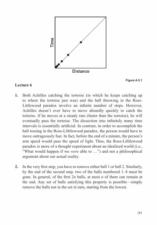
181

Lecture 6

1. Both Achilles catching the tortoise (in which he keeps catching up to where the tortoise just was) and the ball throwing in the Ross-Littlewood paradox involve an infinite number of steps. However, Achilles doesn’t ever have to move absurdly quickly to catch the tortoise. If he moves at a steady rate (faster than the tortoise), he will eventually pass the tortoise. The dissection into infinitely many time intervals is essentially artificial. In contrast, in order to accomplish the ball tossing in the Ross-Lilttlewood paradox, the person would have to move outrageously fast. In fact, before the end of a minute, the person’s arm speed would pass the speed of light. Thus, the Ross-Lilttlewood paradox is more of a thought experiment about an idealized world (i.e., “What would happen if we were able to …”) and not a philosophical argument about our actual reality.

2. In the very first step, you have to remove either ball 1 or ball 2. Similarly, by the end of the second step, two of the balls numbered 1–4 must be gone. In general, of the first 2n balls, at most n of them can remain at the end. Any set of balls satisfying this property is possible—simply remove the balls not in the set in turn, starting from the lowest.

Figure A.5.1

182

Solu

tions

Lecture 7

1. The following is one such list.

1. 1.0000000… (this number is equal to 0.1)

2. 0.3434122…

3. 0.5254643…

4. 3.1414926…

If we continue this list with the diagonal entries all non-9’s, then the diagonal entries would form this number: 0.0454….

Applying our algorithm, we’d form the number 0.999999…, which already appears on our list in the first position (as 1.00000…).

2. The key problem is that the number resulting from the diagonalization argument must be in the set in question; the contradiction comes because that number is missing, so the function missed a number that it supposedly included. When you write rational numbers as decimals, they all either terminate or repeat (i.e., 1/5 = 0.2, 1/7 = 0.14285714285714…). If you apply the diagonal argument to the rational numbers, the resulting number isn’t rational (i.e., it neither terminates nor repeats), so you cannot conclude that the function missed a rational number.

Lecture 8

1. One way mathematicians think about dimension is about the degrees of freedom allowed within a space. A line allows only 1 degree of freedom: You can travel forward or back as many units as you wish, but no other motion is possible. A plane allows 2 degrees of freedom, which is why we typically describe planes in terms of 2 variables, usually x and y.

183

Another method relies on circles, spheres, and higher-dimensional analogs, asking the question, can you cover a set with countably many of these objects? If the answer is yes for spheres, then the object has dimension 3 or less. If the object is coverable by countably many spheres, but not by countably many circles, then the dimension is greater than 2, but not more than 3. There are several different formulations of the details (the most common being Hausdorff dimension), but interestingly, all allow for objects with non-integer dimension.

2. In a recent paper, Fernando Gouvêa makes a convincing argument that Cantor didn’t doubt the truth of the statement he had proved, but instead only had doubts (which proved to be well founded) about the completeness of his proof.

Lecture 9

1. There is a smallest number that isn’t in this set. So, that number is not defined by a finite definition. But “the smallest number not defined by a finite definition” would then be a finite definition of this element. This is König’s paradox, first published in 1905 by Hungarian mathematician Julius König. Note that the ordering used in this paradox is different from the usual ordering of the real numbers; it’s more closely related to the well-ordering theorem, which is equivalent to the axiom of choice.

2. A universal set, U, would include every possible element and every possible set. In fact, it would include every element that is contained in every set that it includes. For example, if set A is in U, and element x is in A, then because U contains all possible elements, it also contains x. (In other words, U = {A, x, ….}.) Because this happens with every set contained in U, this violates the axiom of regularity; there is no non-empty set in U that is disjoint from U.

184

Solu

tions

Lecture 10

1. •• The first sentence is not contradictory. Either it follows from the axioms of the system (in which case it is provable—and thus true), or it doesn’t (in which case it is not provable—and thus false). There is no contradiction either way.

•• This is more complicated. It turns out that the statement “Q is the Gödel number of a false formula” cannot be represented as a formula of arithmetic. This was discovered independently by Gödel and Tarski, and it is known as Tarski’s undefinability theorem.

Lecture 11

1. a) Nobody (A has the most votes with 3).

b) A with 3 votes (E has 2; C and D have 1 each).

c) C with 4 votes (E has 3; A and D have 2; B has 1).

d) E with 19 points (C has 17; D has 15).

e) A wins (after C and D are dropped from counting).

f) A wins.

g) Yes. A beats all other candidates in 1-on-1 matchups.

2. In this case, the positions are symmetrical. Whoever is chair will end up with his or her least-favorite outcome as the result. To get her top choice (Brazilian), Rebecca has to put the person with Brazilian as their last choice in power. She should abdicate her chair position to Steve.

185

Lecture 12

1. In addition to being the “fairest” in the sense that no switching makes any difference of representation any smaller, the Huntington-Hill method avoids the most problematic of the paradoxes, including the Alabama paradox and the new state paradox. While it occasionally fails the quota rule (as do all methods that avoid the other paradoxes), that rule is now seen as too restrictive. Failing the quota rule, while counterintuitive, is not seen as a fatal flaw of an apportionment method. Additionally, in practice, the Huntington-Hill method frequently produces exactly the same results as Webster’s method.

2. If a = b, then they are equal. If not, the arithmetic mean is always greater than the geometric mean. Why?

0 < (a − b)2

= a2 − 2ab + b2

= a2 + 2ab + b2 − 4ab

= (a + b)2 − 4ab

Thus, 4ab < (a + b)2, and taking square roots gives the desired inequality.

Lecture 13

1. For 39 days, nothing happens. On the 40th day, all the brown-eyed people leave. The reasoning is the same as for the problem given in the lecture (involving 100 blue-eyed people and nobody else). On the 39th day, all the brown-eyed people learn new information—that there aren’t just 39 brown-eyed people on the island. On the same day, the blue-eyed people “learn” something, too—that there aren’t just 39 blue-eyed people on the island. Of course, because each of them sees 59 blue-eyed people, that isn’t new information.

186

Solu

tions

2. With 2 pirates, the youngest now proposes to keep everything, with a 1-to-1 tie giving him all the loot. With 3 pirates, the youngest only needs to buy the oldest’s vote with 1 coin, so he proposes 1 for the oldest and 99 for himself (and the plan wins 2 to 1). With 4 pirates, the youngest can buy the 2nd oldest most cheaply (because with 3 pirates, he’d be left with nothing), so he proposes 1 coin for the 2nd oldest and keeps the rest on a 2-to-2 vote. Finally, with 5 pirates, the youngest can cheaply buy the votes of the oldest and the middle pirates for 1 coin each, saving 98 coins for himself (and winning the vote 3 to 2).

Lecture 14

1. The following is one way that will save the 3 more than 50% of the time.

•• See 2 reds? Guess blue.

•• See 1 red? Pass.

•• See no reds? Guess red.

If you write out the 27 possibilities, this strategy wins 15 times, more than 55% of the time.

2. The first person to guess can still pass enough information to the others to save them all. If he or she adds up the colors of the hats he or she sees, divides by n and takes the remainder, and guesses the color associated with that number, the person in front of him or her can figure out his or her own hat color. (The colors he or she sees plus his or her own hat color have to add up to the color guessed by the first person.) Everyone in front of him or her hears his or her guess and can thus determine the sum of all the hats in front of him or her plus his or her own (modulo n). This allows each person to determine his or her own hat color.

187

Lecture 15

1. Even if the short connector road in the figure 8 is open, everyone could choose to ignore it. But then the first person to take that connector would find it very fast—a great improvement over his or her normal route. But if everyone makes that same decision, the route becomes much slower than his or her normal route would have been. By being greedy, everyone gets a worse outcome, just like with the prisoner’s dilemma. (Technically, this is a bit closer to a case of the tragedy of the commons.)

2. Your car’s shock absorbers have a resonant frequency. If the shaking is particularly bad, it means that you are traveling over the bumps at exactly the right rate, so your shocks are being driven at their resonant frequency. Speeding up or slowing down both work because they get off of the peak resonance.

Lecture 16

1. Special relativity doesn’t take into account acceleration. The twin who leaves the Earth has to accelerate up to speed and accelerate again to turn around prior to the return trip. Those accelerations require general relativity to analyze; doing so verifies the twin paradox.

2. We don’t know yet!

Lecture 17

1. The slope of the hypotenuse of the larger triangle is 3/8. The slope of the hypotenuse of the smaller triangle is 2/5. These two aren’t equal, so the two have different slopes, so neither picture is actually a triangle. The top one bulges in, and the bottom one bulges out, and that’s where the “missing” square comes from.

2. Each section of the perimeter is the arc of a circle centered at one of the vertices of the triangle. To see why the shape has constant width, picture the “diameter” that goes through A and C. Rotate that diameter around the point A until it goes through B. Because both ends follow circles

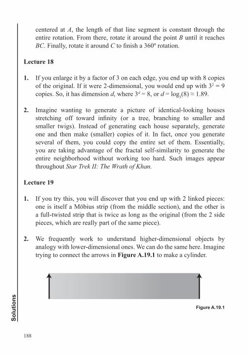
188

Solu

tions

centered at A, the length of that line segment is constant through the entire rotation. From there, rotate it around the point B until it reaches BC. Finally, rotate it around C to finish a 360º rotation.

Lecture 18

1. If you enlarge it by a factor of 3 on each edge, you end up with 8 copies of the original. If it were 2-dimensional, you would end up with 32 = 9 copies. So, it has dimension d, where 3d = 8, or d = log3(8) ≈ 1.89.

2. Imagine wanting to generate a picture of identical-looking houses stretching off toward infinity (or a tree, branching to smaller and smaller twigs). Instead of generating each house separately, generate one and then make (smaller) copies of it. In fact, once you generate several of them, you could copy the entire set of them. Essentially, you are taking advantage of the fractal self-similarity to generate the entire neighborhood without working too hard. Such images appear throughout Star Trek II: The Wrath of Khan.

Lecture 19

1. If you try this, you will discover that you end up with 2 linked pieces: one is itself a Möbius strip (from the middle section), and the other is a full-twisted strip that is twice as long as the original (from the 2 side pieces, which are really part of the same piece).

2. We frequently work to understand higher-dimensional objects by analogy with lower-dimensional ones. We can do the same here. Imagine trying to connect the arrows in Figure A.19.1 to make a cylinder.

Figure A.19.1

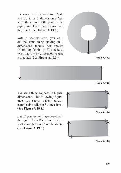
189

It’s easy in 3 dimensions. Could you do it in 2 dimensions? Yes. Keep the arrows in the plane of the paper, and bend them down until they meet. (See Figure A.19.2.)

With a Möbius strip, you can’t do the same thing staying in 2 dimensions—there’s not enough “room” or flexibility. You need to twist into the 3rd dimension to tape it together. (See Figure A.19.3.)

The same thing happens in higher dimensions. The following figure gives you a torus, which you can completely realize in 3 dimensions. (See Figure A.19.4.)

But if you try to “tape together” the figure for a Klein bottle, there isn’t enough “room” or flexibility. (See Figure A.19.5.)

Figure A.19.2

Figure A.19.3

Figure A.19.4

Figure A.19.5

190

Solu

tions

Lecture 20

1. •• 3-torus: What was showed was accurate, but the final stage was omitted, where the top and bottom are glued together. If that had been done, you would have seen layers of copies of Dave above and below the “main” layer and would need those to be correct in perspective. In other words, if you were looking at a version of Dave in the layer above the main layer, you would need to be able to see the bottoms of his feet.

•• Non-orientable 3-manifold: This demonstration was quite accurate, although it clearly involved some video trickery. In particular, if two people were in this space and one of them walked through the twisted connection, then they would both see each other as having flipped left to right.

•• Quarter-turn manifold: Here gravity is a serious problem. If two people had been in the space and one had walked through the twisted connection, then they would be at 90° angles with each other, one oriented normally with respect to the camera and one with either his or her head or feet pointed at the camera (depending on which direction he or she went). Which way would gravity work? Would it simply pull one’s feet toward whichever face of the cube was perpendicular to one’s spine? Then, it would pull those two people in two different directions. If the person went “around” again, gravity would pull one person down toward the (original) floor, but the person who had traveled through the twist twice would now be sucked toward what was the original ceiling. Gravity would need to be very different from what we’re used to.

Lecture 21

1. Instead of removing middle thirds, remove a fraction that decreases with each successive step. If you first remove an interval of length 1/4, then 2 intervals of length 1/16 (removing a total length of 2/16 = 1/8), then 4 intervals of length 1/(26) (removing a total length

191

of 4/(26) = 1/16), and so on, then the total length removed will be 1/4 + 1/8 + 1/6 + 1/32 + … = 1/2. (The last equality holds by using the geometric series formula discussed in Lecture 5.)

2. No. In 1970, Robert Solovay proved that the construction of any non-measurable set is not possible in the Zermelo-Fraenkel axiomatic system without the addition of the axiom of choice.

Lecture 22

1. Essentially, this new construction is the same as the old one, but the endpoints are removed. Those endpoints are all rational, and thus the set of all of them is countable. Removing a countable set of points (the endpoints) from an uncountable one (the original Cantor set) must result in an uncountable set.

2. The end of the argument works like this: Each one of the rotations (the ones that are disjoint) would have the same measure as the original (this is the third assumption about measure—that the measure of a set isn’t affected by a rigid motion). Together, the union of all of those sets gives the unit interval (which has measure 1, by the fourth assumption).

If the sets didn’t partition so nicely, they might overlap in such a way that the first one might have some positive measure (for example, 1/2), the portion of the second one not in the first one might have some smaller positive measure (for example, 1/4), and the portion of the third one not in either of the first two might have some even smaller positive measure (for example, 1/8). Those measures might add up to 1, and we wouldn’t have a contradiction. We arrive at the contradiction only because each set has the same measure, yet infinitely many of them have to add up to 1.

Lecture 23

1. If you take abP and apply a2, you get a3bP = bP. Then, apply b to get b2P = P. Finally, apply a to get aP = N. In other words, aba2abP = abbP = aP = N.

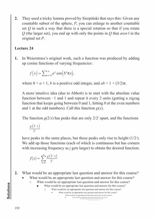
192

Solu

tions

2. They used a tricky lemma proved by Sierpiński that says this: Given any countable subset of the sphere, P, you can enlarge to another countable set Q in such a way that there is a special rotation so that if you rotate Q (the larger set), you end up with only the points in Q that aren’t in the original set P.

Lecture 24

1. In Weierstrass’s original work, such a function was produced by adding up cosine functions of varying frequencies:

f x a b xcos ,n nn 0∑ ( )( )= =

∞ π

where 0 < a < 1, b is a positive odd integer, and ab > 1 + (3/2)π.

A more intuitive idea (due to Abbott) is to start with the absolute value function between −1 and 1 and repeat it every 2 units (getting a zigzag function that keeps going between 0 and 1, hitting 0 at the even numbers and 1 at the odd numbers). Call this function g(x).

The function g(2 jx) has peaks that are only 2/2 j apart, and the functions

g x22

j

j

( )

have peaks in the same places, but those peaks only rise to height (1/2 j). We add up those functions (each of which is continuous but has corners with increasing frequency as j gets larger) to obtain the desired function:

f x g x22n 0

j

j∑ ( )=

=

∞

2. What would be an appropriate last question and answer for this course?•• What would be an appropriate last question and answer for this course?

○• What would be an appropriate last question and answer for this course?■• What would be an appropriate last question and answer for this course?

□• What would be an appropriate last question and answer for this course?•• What would be an appropriate last question and answer for this course?

○• What would be an appropriate last question and answer for this course?■• What would be an appropriate last question and answer for this course?

□• What would be an appropriate last question and answer for this course?•• What would be an appropriate last question and answer for this course?

193

Bibliography

Al-Khalili, Jim. Paradox: The Nine Greatest Enigmas in Physics. New York: Random House, 2012. An intriguing tour of nine different paradoxes, written by a physicist for a general audience, with sections on Zeno’s paradoxes and many modern physics conundrums.

Balinski, Michel L., and H. Peyton Young. Fair Representation: Meeting the Ideal of One Man, One Vote. Washington, DC: Brookings Institution Press, 2001. A thorough look at the many methods and paradoxes of reapportionment.

Belmont, Barry. “NSF Fluid Mechanics Series: 18. Stratified Flow.” YouTube video, 27:00. April 28, 2011. https://www.youtube.com/watch?v=9hmjcIfy8wE&list=PL0EC6527BE871ABA3&index=19. Created by the National Committee for Fluid Mechanics Films half a century ago, this video is part of a series designed to explain fluid mechanics to the public. The section on the dead water phenomenon starts at the 12:28 mark.

Bunch, Bryan. Mathematical Fallacies and Paradoxes. Mineola, NY: Courier Dover Publications, 2012. Great examples of “proving” impossible statements (such as 0 = 1) along with very complete explanations.

Cohen, I. Bernard. Science and the Founding Fathers: Science in the Political Thought of Jefferson, Franklin, Adams and Madison. New York: W. W. Norton & Company, 1995. A science-based perspective on early American history, including a look at the founding fathers’ apportionment battles.

Dauben, Joseph W. Georg Cantor: His Mathematics and Philosophy of the Infinite. Princeton, NJ: Princeton University Press, 1990. A fascinating biography of the great mathematician, putting his work in a clearer personal, professional, and historical context.

194

Bib

liogr

aphy

Dawkins, Richard. The Selfish Gene. Oxford: Oxford University Press, 2006. This classic of evolutionary biology includes an extensive discussion of the prisoner’s dilemma and how the iterated version models some evolutionary processes.

Dunham, William. Journey through Genius: The Great Theorems of Mathematics. New York: Wiley, 1990. This tour through different mathematicians and their brilliant works includes an extensive section on Georg Cantor.

Gardner, Martin. Aha! Gotcha: Paradoxes to Puzzle and Delight. San Francisco, CA: W. H. Freeman, 1982. This classic collection of Gardner’s work includes a discussion of the two envelopes problem, phrased in terms of two men comparing the contents of their wallets.

———. Hexaflexagons and Other Mathematical Diversions: The First Scientific American Book of Puzzles and Games. Chicago: University of Chicago Press, 1988. Another classic Gardner collection, including an in-depth discussion of the one-mile-south puzzle.

———. Penrose Tiles to Trapdoor Ciphers: And the Return of Dr. Matrix. Cambridge: Cambridge University Press, 1997. Another collection of Gardner’s columns, including a discussion of many variations of hat games.

———. The Unexpected Hanging and Other Mathematical Diversions. New York: Simon and Schuster, 1969. This classic of recreational mathematics includes an extensive discussion of the unexpected hanging paradox.

———. Wheels, Life, and Other Mathematical Amusements. New York: W. H. Freeman, 1983. This Gardner collection includes an extended discussion of the puzzles of Sam Lloyd.

Gorroochurn, Prakash. Classic Problems of Probability. New York: John Wiley & Sons, 2012. Many great examples of surprising and paradoxical problems in probability, including Bertrand’s chord problem, all with complete (at times advanced) mathematical details.

195

Gould, Stephen Jay. Full House. Cambridge, MA: Harvard University Press, 2011. A collection of great science essays, including a detailed look at baseball players hitting .400.

Gribbin, John. In Search of Schrodinger’s Cat: Quantam Physics and Reality. New York: Random House, 2011. An overview of quantum physics, including many of its paradoxes, written for a general audience.

Groopman, Jerome, and Pamela Hartzband. Your Medical Mind: How to Decide What Is Right for You. London: Penguin, 2011. A readable analysis of medical statistics and how you should interpret them.

Huff, Darrell. How to Lie with Statistics. New York: W. W. Norton & Company, 2010. Simply a classic, including many great examples of how statistics can be twisted to mislead.

Mandelbrot, Benoit B. The Fractal Geometry of Nature. New York: W. H. Freeman, 2010. The seminal book on fractals, from the researcher who coined the term.

MatthieuMercier’s channel. “Dead Water Phenomenon (‘toy box’).” YouTube video, 2:57. May 21, 2009. https://www.youtube.com/watch?v=bzcgAshAg2o. A modern video showing the dead water effect of interfacial waves, including close-ups of the wave catching up to the boat and the same phenomenon with three liquid layers.

Mlodinow, Leonard. The Drunkard’s Walk: How Randomness Rules Our Lives. New York: Random House, 2009. A popular account of how randomness arises in everyday life, including examples of the prosecutor’s fallacy.

Moore, Gregory H. Zermelo’s Axiom of Choice: Its Origins, Development, and Influence. Mineola, NY: Courier Dover Publications, 2012. A complete account of early set theory, written for a mathematically sophisticated reader.

196

Bib

liogr

aphy

Nagel, Ernest, and James Roy Newman. Gödel’s Proof. Edited by Douglas R. Hofstadter. New York and London: New York University Press, 2001. A modern update of a 1950s classic, containing an accessible yet complete explanation of Gödel’s seminal work.

Niederman, Derrick, and David Boyum. What the Numbers Say: A Field Guide to Mastering Our Numerical World. New York: Random House, 2007. A captivating look at how numbers are used to convince and mislead us, including a section on gas mileage.

NPR. “Episode 443: Don’t Believe The Hype.” Planet Money podcast. March 12, 2013. http://www.npr.org/blogs/money/2013/03/12/174139347/episode-443-dont-believe-the-hype. An excellent explanation of the deeply mathematical averaging flaws of the Dow Jones Industrial Average.

Pearl, Judea. Causality. Cambridge: Cambridge University Press, 2009. Written by a computer scientist/philosopher, this mathematically sophisticated book includes an extensive discussion of Simpson’s paradox.

Pickover, Cliff. Every Insanely Mystifying Paradox in Physics: A Complete List. http://sprott.physics.wisc.edu/pickover/physics-paradoxes.html. Accessed May 27, 2014. An exhaustive (and exhausting) list of paradoxes in classical and modern physics, from a prolific general interest math and science writer.

Rosenhouse, Jason. The Monty Hall Problem: The Remarkable Story of Math’s Most Contentious Brain Teaser. Oxford: Oxford University Press, 2009. An excellent, readable review of the probability needed to understand the boy/girl problems as well as the Monty Hall problem.

Roughgarden, Tim. Selfish Routing and the Price of Anarchy. Cambridge, MA: MIT Press, 2005. An interesting, technical look at the problems of individuals making selfish choices, including a discussion of the implications of Braess’s paradox.

197

Saari, Donald. Chaotic Elections! A Mathematician Looks at Voting. Providence, RI: American Mathematical Society, 2001. Written by a Great Courses professor, this book elucidates, among other things, the intuition of Arrow’s theorem.

Salmon, Wesley C., ed. Zeno’s Paradoxes. Indianapolis, IN: Hackett Publishing, 1970. A collection of essays including historical, mathematical, and philosophical perspectives on Zeno’s famous paradoxes.

Smullyan, Raymond M. Satan, Cantor, and Infinity: And Other Mind-Boggling Puzzles. New York: Random House, 2012. A classic in logic puzzles, beginning with knights and knaves problems and moving quickly into infinity, eventually tackling Gödel’s groundbreaking work.

———. The Lady or the Tiger? And Other Logic Puzzles. Mineola, NY: Courier Dover Publications, 2009. A newer puzzle book in the same vein as Smullyan’s first book, again starting with fairly simple logic puzzles and increasing in complexity.

———. What Is the Name of This Book? Englewood Cliffs, New Jersey: Prentice-Hall, 1978. Smullyan’s first book starts from the basic liar’s paradox and branches into many original knights and knaves problems, including some very complicated ones.

ssgelm. “Outside In.” YouTube video, 21:25. April 23, 2011. https://www.youtube.com/watch?v=wO61D9x6lNY. The Geometry Center’s mini-documentary explaining the sphere eversion problem (turning the sphere inside out) and a graphical demonstration of its solution.

Stewart, Ian. Math Hysteria: Fun and Games with Mathematics. Oxford: Oxford University Press, 2004. One of the Scientific American writer’s many contributions to recreational mathematics, this book includes an extended discussion of the pirate game, and a version of the brown-eyed/blue-eyed islanders puzzle.

198

Bib

liogr

aphy

University of Adelaide. “Official Parrondo’s Paradox Page.” School of Electrical and Electronic Engineering. Accessed May 27, 2014. http://www.eleceng.adelaide.edu.au/Groups/parrondo/. A compendium of examples and explanations (some technical) of Parrondo’s paradox.

Veritasium. “Slinky Drop Answer.” YouTube video, 3:30. September 21, 2011. https://www.youtube.com/watch?v=eCMmmEEyOO0. A slow-motion version of the Slinky experiment, with explanation and links to related experiments (with larger Slinkies and Slinkies with weights attached).

Wagon, Stan. The Banach-Tarski Paradox. Vol. 24. Cambridge: Cambridge University Press, 1993. A book on the theorem presented by Stefan Banach and Alfred Tarski in 1924.

Wapner, Leonard M. The Pea and the Sun: A Mathematical Paradox. Wellesley, MA: A. K. Peters, Ltd., 2005. An extended look at the Banach-Tarski paradox, from its historical underpinnings to its strange implications, written for a general audience.

Weeks, Jeffrey R. The Shape of Space. Boca Raton, FL: CRC Press, 2001. A brilliantly written exploration of basic and advanced topological concepts, from orientability to higher-dimensional manifolds, written by a MacArthur “genius grant” winner.

Notes

Notes