Millimeter wave massive MIMO beamforming communication ...cj82ss44c/fulltext.pdfMillimeter Wave...

Millimeter Wave Massive MIMO beamforming communication

simulator design: a systematic approach

A Thesis Presented

by

Zhengnan Li

to

The Department of Electrical and Computer Engineering

in partial fulfillment of the requirements

for the degree of

Master of Science

in

Electrical and Computer Engineering

Northeastern University

Boston, Massachusetts

July 2018

To my family – without whom I would not have the chance of seeing a better world.

To my friends during masters’ – Amanda, Spark, Mingyu, Ken, for your generous support throughout.

To Tiansu – happy belated birthday, and sincerely wish you the best in your endeavors.

i

Contents

List of Figures iv

List of Tables v

Acknowledgments viii

Abstract of the Thesis ix

1 Introduction 1

2 Introduction to 802.11ad Physical Layer 32.1 802.11ad Single Carrier PHY Frame Format . . . . . . . . . . . . . . . . . . . . . 32.2 Common parameters and requirements for 802.11ad . . . . . . . . . . . . . . . . . 4

3 Introduction to 3GPP Technical Report 38.901 Channel Models 53.1 Methodology in Generating Channel Coefficients . . . . . . . . . . . . . . . . . . 5

3.1.1 Set environment, network layout and antenna array parameters . . . . . . . 53.1.2 Set (Non) Line of Sight probability and pathloss . . . . . . . . . . . . . . 53.1.3 Set small-scale parameters, including delay spread, angular spreads, cross

polarization ratio, cluster delays, powers, arrival and departure angle . . . . 63.1.4 Draw initial phases and generate channel coefficients . . . . . . . . . . . . 83.1.5 Apply pathloss, shadowing and the channel coefficients to the input signal . 10

3.2 Example Results . . . . . . . . . . . . . . . . . . . . . . . . . . . . . . . . . . . 10

4 802.11ad Receiver Reference Design and Performance Analysis 134.1 DMG packet detection . . . . . . . . . . . . . . . . . . . . . . . . . . . . . . . . 134.2 Frequency offset estimation . . . . . . . . . . . . . . . . . . . . . . . . . . . . . . 144.3 Channel Estimation and Equalization . . . . . . . . . . . . . . . . . . . . . . . . . 144.4 Receiver state machine . . . . . . . . . . . . . . . . . . . . . . . . . . . . . . . . 144.5 PER performance of 3GPP recommended channel . . . . . . . . . . . . . . . . . . 154.6 MCS selection mechanism . . . . . . . . . . . . . . . . . . . . . . . . . . . . . . 17

5 Introduction to Beamforming 185.1 What is beamforming? . . . . . . . . . . . . . . . . . . . . . . . . . . . . . . . . 18

ii

5.2 Bartlett’s Beamformer (Conventional) . . . . . . . . . . . . . . . . . . . . . . . . 185.3 Capon’s Beamformer (Minimum Variance Distortionless Response (MVDR)) . . . 195.4 Frost’s Beamformer (Linear-Constrained Minimum Variance (LCMV)) . . . . . . 20

5.4.1 Distortionless Constraint . . . . . . . . . . . . . . . . . . . . . . . . . . . 205.4.2 Directional Constraint . . . . . . . . . . . . . . . . . . . . . . . . . . . . 205.4.3 Null Constraint . . . . . . . . . . . . . . . . . . . . . . . . . . . . . . . . 21

6 Beamforming Enabled Massive MIMO Physical Layer Simulations 226.1 Phased array processors – radiators, collectors, steering vectors . . . . . . . . . . . 23

6.1.1 Radiators and collectors . . . . . . . . . . . . . . . . . . . . . . . . . . . 236.1.2 Steering Vectors . . . . . . . . . . . . . . . . . . . . . . . . . . . . . . . 236.1.3 Array Response . . . . . . . . . . . . . . . . . . . . . . . . . . . . . . . . 23

6.2 Simulator architecture . . . . . . . . . . . . . . . . . . . . . . . . . . . . . . . . . 246.3 Simulation Results . . . . . . . . . . . . . . . . . . . . . . . . . . . . . . . . . . 25

7 Conclusion 28

Bibliography 29

iii

List of Figures

2.1 SC PHY frame format . . . . . . . . . . . . . . . . . . . . . . . . . . . . . . . . 4

3.1 Pathloss vs Distance (Indoor office) . . . . . . . . . . . . . . . . . . . . . . . . . 73.2 Example of CDL-C Channel (delay) . . . . . . . . . . . . . . . . . . . . . . . . . 103.3 Example of CDL-C Channel (tap) . . . . . . . . . . . . . . . . . . . . . . . . . . 103.4 Example of CDL-D Channel (delay) . . . . . . . . . . . . . . . . . . . . . . . . . 103.5 Example of CDL-D Channel (tap) . . . . . . . . . . . . . . . . . . . . . . . . . . 10

4.1 Channel Estimation Performance . . . . . . . . . . . . . . . . . . . . . . . . . . . 154.2 Receiver State Machine . . . . . . . . . . . . . . . . . . . . . . . . . . . . . . . . 164.3 PER of CDL-C (NLoS) Profile . . . . . . . . . . . . . . . . . . . . . . . . . . . . 174.4 PER of CDL-D (LoS) Profile . . . . . . . . . . . . . . . . . . . . . . . . . . . . . 17

5.1 Normalized Power of LCMV beamformer with specified requirements . . . . . . . 21

6.1 PER of LCMV beamformer with 4 users, CDL-C, fixed user position . . . . . . . . 256.2 PER of LCMV beamformer with 4 users, CDL-C, random user position . . . . . . 256.3 PER of LCMV beamformer with 128 antennas, CDL-C, fixed user position . . . . 266.4 PER of LCMV beamformer with 128 antennas, CDL-C, random user position . . . 266.5 PER of heuristics beamformer with 4 users, CDL-C, fixed user position . . . . . . 266.6 PER of heuristics beamformer with 128 antennas, CDL-C, fixed user position . . . 26

iv

List of Tables

2.1 (Part of) Timing-related parameters of 802.11ad . . . . . . . . . . . . . . . . . . . 4

3.1 CDL-C Profile (NLoS) . . . . . . . . . . . . . . . . . . . . . . . . . . . . . . . . 113.2 CDL-D Profile (LoS) . . . . . . . . . . . . . . . . . . . . . . . . . . . . . . . . . 12

v

Acronyms

3GPP 3rd Generation Partnership Project.

AGC Automatic Gain Control.AoA Azimuth angle of Arrival.AoD Azimuth angle of Departure.AP Access Point.ASA Azimuth angle Spread of Arrival.ASD Azimuth angle Spread of Depature.AWGN Additive White Gaussian Noise.AWV Antenna Weight Vector.

BF Beamforming Field.

CA Carrier Sensing.CCA Clear Channel Assessment.CDL Clustered Delay Line.CEF Channel Estimation Field.CIR Channel Impluse Response.

DF Data Field.DMG Directional multi-gigabit.DoA Direction of Arrival.DoF Degree of Freedom.

FDE Frequency Domain Equalization.FIR Finite Impulse Response.

GCS Global Coordinate System.

LCMV Linear-Constrained Minimum Variance.LCS Local Coordinate System.LDPC Low Density Parity Check.LoS Line of Sight.LUT Look Up Table.

vi

MAC Medium Access Control Layer.MCS Modulation and Coding Scheme.MIMO Multiple Input Multiple Output.ML Maximum Likelihood.MPC MultiPath Cluster.MSE Mean Squared Error.MVDR Minimum Variance Distortionless Response.

NLoS Non Line of Sight.

OFDM Orthogonal Frequency-Division Multiplexing.

PDP Power Delay Profile.PER Packet Error Rate.PHY Physical Layer.PPDU PLCP Protocol Data Unit.PSDU PLCP Service Data Unit.

QoS Quality of Service.

RMS Rooted Mean Square.RSS Received Signal Strength.

SC Single Carrier.SNR Signal to Noise Ratio.STA Station.STF Short Training Field.

TRN-T/R Training Field (Transmit/Receive).

ULA Uniform Linear Array.

XPR Cross Polarization Ratio.

ZoA Zenith angle of Arrival.ZoD Zenith angle of Departure.ZSA Zenith angle Spread of Arrival.ZSD Zenith angle Spread of Depature.

vii

Acknowledgments

I would like to express my gratitude to my advisor Prof. Chowdhury for his generoussupport, his encouragement throughout my master’s study, and patience in guiding me on technicalissues. His academical excellence, his dedication, and his passion for research will always enlightenme furthering my studies in wireless communications.

I would also like to thank all my colleagues both in lab and at the MathWorks – Miad,Parisa, Munish, Amir, Yashar, Stella, Kunal, and Mike, Ethem, Tasos, Yue – without your help andguidance this work wouldn’t finish. It is always my pleasure to exchange ideas with you and thoseideas always shine. Besides, thanks to Haoran, Wangbo, Ruixiao on their supports.

Special thanks to Prof. Stojanovic, from whom I learn how to be a researcher and a positiveobserver.

viii

Abstract of the Thesis

Millimeter Wave Massive MIMO beamforming communication simulator

design: a systematic approach

by

Zhengnan Li

Master of Science in Electrical and Computer Engineering

Northeastern University, July 2018

Dr. Kaushik R. Chowdhury, Advisor

With the growth of data traffic demands, wireless network architectures that use traditionalsub-6 GHz frequency bands are now reaching their capacities. Millimeter wave (mmWave) com-munication is a transformative paradigm given its potential to attain throughput that goes beyondseveral gigabits per second, with over 2-4GHz of bandwidth. However, it also incurs high levelsof signal attenuation that raises challenges in connectivity with increasing distance. The relativelyhigh pathloss can be mitigated via beamforming technique, where signal energy is directed towards aspecific user or target by appropriately weighting the phases of the antenna elements. In addition,the comparatively small millimeter wavelength also allows practicability of employing massiveantenna elements within a small surface area. Thus, so called ‘massive’ clusters of antenna elementsare now possible. This thesis presents a systematic simulator design for mmWave-based networkarchitectures, fulfilling the requirements of next generation of telecommunication (5G).

In this thesis, a beamforming enabled massive multiple input multiple output (MIMO)based physical (PHY) layer simulator design is proposed and implemented in MATLAB. It consistsof IEEE 802.11ad standard compliant transceiver design, 3GPP TR 38.901 channel model, andbeamforming performance evaluation platform. The simulator facilitates assessment of differentbeamforming algorithms, as well as Medium Access Control (MAC) layer design process. Alongwith the transceiver, a Modulation and Coding Scheme (MCS) selection mechanism is also proposedto guarantee timing and throughput requirements from upper layer. Packet Error Rate (PER) resultsof the transceiver is simulated with different Clustered Delay Line (CDL) profiles suggested by TR38.901.

ix

Chapter 1

Introduction

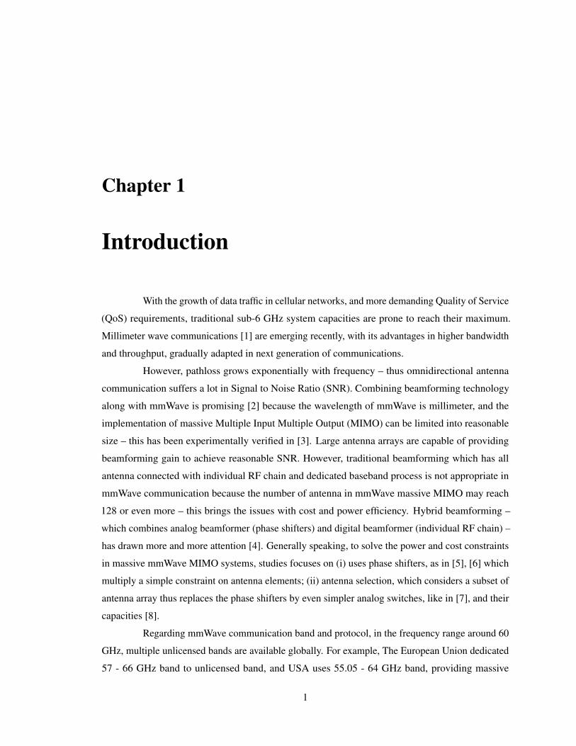
With the growth of data traffic in cellular networks, and more demanding Quality of Service

(QoS) requirements, traditional sub-6 GHz system capacities are prone to reach their maximum.

Millimeter wave communications [1] are emerging recently, with its advantages in higher bandwidth

and throughput, gradually adapted in next generation of communications.

However, pathloss grows exponentially with frequency – thus omnidirectional antenna

communication suffers a lot in Signal to Noise Ratio (SNR). Combining beamforming technology

along with mmWave is promising [2] because the wavelength of mmWave is millimeter, and the

implementation of massive Multiple Input Multiple Output (MIMO) can be limited into reasonable

size – this has been experimentally verified in [3]. Large antenna arrays are capable of providing

beamforming gain to achieve reasonable SNR. However, traditional beamforming which has all

antenna connected with individual RF chain and dedicated baseband process is not appropriate in

mmWave communication because the number of antenna in mmWave massive MIMO may reach

128 or even more – this brings the issues with cost and power efficiency. Hybrid beamforming –

which combines analog beamformer (phase shifters) and digital beamformer (individual RF chain) –

has drawn more and more attention [4]. Generally speaking, to solve the power and cost constraints

in massive mmWave MIMO systems, studies focuses on (i) uses phase shifters, as in [5], [6] which

multiply a simple constraint on antenna elements; (ii) antenna selection, which considers a subset of

antenna array thus replaces the phase shifters by even simpler analog switches, like in [7], and their

capacities [8].

Regarding mmWave communication band and protocol, in the frequency range around 60

GHz, multiple unlicensed bands are available globally. For example, The European Union dedicated

57 - 66 GHz band to unlicensed band, and USA uses 55.05 - 64 GHz band, providing massive

1

CHAPTER 1. INTRODUCTION

opportunities of achieving multi-gigabit transmission rate. However, the primary challenge with

60GHz band communication is that the pathloss is much poorer than those in the sub-6 GHz bands

– the free-space pathloss at 1m for 60 GHz is 68dB whereas 47 dB at 5 GHz. The IEEE 802.11ad

protocol [9] uses a so called Directional multi-gigabit (DMG) packet, whose aim is to beamform

towards desired direction to provide gigabyte bandwidth communication link. The DMG Physical

Layer (PHY) supports three modulation methods, a control modulation using Modulation and Coding

Scheme (MCS) 0; a single carrier modulation using MCS 1 to MCS 12; and an Orthogonal Frequency-

Division Multiplexing (OFDM) modulation using MCS 13 to MCS 25. This paper will focus on

Single Carrier (SC) 802.11ad communication link simulations.

To simulate a complete communication link, the channel between transmitter and receiver

is required. The 3rd Generation Partnership Project (3GPP) released a technical report, named Study

on Channel Model for Frequencies from 0.5 to 100GHz, labeled 3GPP TR 38.901 [10], described

and summarized a systematic method in modeling and evaluate the performance of physical layer

techniques, by simulating the radio channel. This model suggests series of key parameters describing

a relative complete scenario, from pathloss to large scale fading, reaching finally at small scale

parameters.

Finally, this thesis presents a massive MIMO mmWave beamforming communication

link simulator, by introducing its components in the following chapter, namely, 802.11ad PHY

introduction, 3GPP TR 38.901 channel model summarization, 802.11ad PHY receiver reference

design and its Packet Error Rate (PER) performance, introduction to beamforming, and the last

chapter states the integrated simulator design.

The main contribution of this thesis lies in the proposed integrated beamforming-communication

simulator, for its usages in beamforming algorithm evaluation, mmWave PHY/Medium Access Con-

trol Layer (MAC) layer co-design etc. This thesis first presents the PER results under different 3GPP

TR 38.901 channel model Clustered Delay Line (CDL) profiles, and then presents the PER results of

different beamformers to demonstrate their performance.

2

Chapter 2

Introduction to 802.11ad Physical Layer

2.1 802.11ad Single Carrier PHY Frame Format

As shown in Figure 2.1, the single carrier PHY contains several fields, itemizing,

• Short Training Field (STF) is composed of 16 repetitions of Golay sequences of length 128,

Ga128(n), followed by a single repetition of −Ga128(n).

• Channel Estimation Field (CEF) is used for channel estimation and the indication of mod-

ulation. The CEF composes two sequences, Gu512(n) and Gv512(n), where Gu512 =

[−Gb128,−Ga128, Gb128,−Ga128], and Gv512 = [−Gb128, Ga128,−Gb128,−Ga128]. Note

that Gb128 is also a Golay sequence of length 128. For single carrier packets, the format of

this channel estimation field is different from that in OFDM packet. Because of the good auto-

correlation property of the Golay sequence, it enables the reconstruction of Channel Impluse

Response (CIR) between the transmitter and the receiver – a summation of autocorrelations of

Ga128 and Gb128 is the Dirac delta function – naturally formulates CIR.

• Header consists of several fields that define of the details of PLCP Protocol Data Unit (PPDU)

to be transmitted later, e.g., MCS, length of PPDU etc.

• Data Field (DF) composes the payload data of the PLCP Service Data Unit (PSDU) and possible

padding. The data after padding with zeros are then scrambled, encoded, and modulated as

dictated by MCS, the modulation and coding scheme. The scrambler uses a polynomial

S(x) = x7 + x4 + 1, generating a periodic sequence of length 127. The data are then encoded

by a systematic Low Density Parity Check (LDPC) encoder.

3

CHAPTER 2. INTRODUCTION TO 802.11AD PHYSICAL LAYER

Short Training Field Channel Estimation Field Header Data ... AGC Subfields TRN-R/T Subfields

Figure 2.1: SC PHY frame format

• (Optional) Beamforming Field (BF), including Automatic Gain Control (AGC) field, and

Training Field (Transmit/Receive) (TRN-T/R). Beamforming enables both Tx-Rx side to train

their transmit and receive antenna for better communication conditions (power). In the AGC

field, it composes several repetitions of Golay sequence. The TRN-T/R field consists Golay

sequence, but applied with different Antenna Weight Vector (AWV) to beamform towards

different direction.

2.2 Common parameters and requirements for 802.11ad

The following section lists several parameters and requirements for transceivers,

• Receiver sensitivity, for MCS 0, the PER shall be less than 5% for a PSDU length of 256

bytes, and less than 1% for other MCSs with a PSDU length of 4096 octets, depending their

corresponding input levels.

• Timing related parameters. Table 2.1 states part of timing-related constants of 802.11ad

protocol. Note that this table contains parameters describing SC PHY.

Parameter Value

Fc: SC chip rate 1760 MHz

Tc: SC chip time 0.57ns = 1/Fc

Tseq 72.7ns = 128× TcTSTF : short training field duration 1236ns = 17× TseqTCE : channel estimation field duration 655ns = 9× TseqTHEADER: header duration 0.582µs = 2××TcTData (NBLKS × 512 + 64)× Tc

Table 2.1: (Part of) Timing-related parameters of 802.11ad

Note that the NBLKS is the number of symbol blocks in the procedure of LDPC encoding.

4

Chapter 3

Introduction to 3GPP Technical Report

38.901 Channel Models

The following steps are required in simulation such channel, namely,

3.1 Methodology in Generating Channel Coefficients

3.1.1 Set environment, network layout and antenna array parameters

• Set simulation environment, e.g., rural outdoor area.

• Set the number of Access Point (AP) and Station (STA).

• Give 3D location, antenna pattern, and array orientations of the AP and STA.

• Give STA’s speed and direction of motion

• Specify system center frequency and sample rate according to 802.11ad protocol, here the

center frequency of 802.11ad is 60.48 GHz, and the sample rate is 1760 MSa/s

3.1.2 Set (Non) Line of Sight probability and pathloss

• Assign propagation conditions, meaning to set Line of Sight (LoS) or Non Line of Sight

(NLoS) uncorrelated conditions to each AP-STA pairs, based on simulation scenario. In this

simulator, we assume indoor mixed office setting, and the LoS probability is stated in Equation

3.1,

5

CHAPTER 3. INTRODUCTION TO 3GPP TECHNICAL REPORT 38.901 CHANNEL MODELS

PLoS =

1, d2D ≤ 1.2m

exp(−d2D−1.2

4.7

), 1.2m < d2D < 6.5m

exp(−d2D−6.5

32.6

), 6.5m < d2D

(3.1)

The method of determining LoS or NLoS is by generating a uniformly distributed number in

[0, 1], if this number is less than PLoS, then we claim this pair of AP-STA is of LoS condition.

• Calculate pathloss for each AP-STA link to be modeled, by Equation 3.2, of the LoS pathloss

PLIn-LoS(dB) = 32.4+17.3 log10 (d3D)+20 log10 (fc)+∆gLoS, 1m ≤ d3D ≤ 100m (3.2)

where ∆gLoS conforms log-normal distribution with 0 mean, 3 dB variance.

For NLoS conditions, they are stated in Equation 3.3,

PLIn-NLoS(dB) = max{PLIn-LoS, PL

′In-NLoS

}(3.3)

where,

PL′In-NLoS = 38.3 log10(d3D) + 17.30 + 24.9 log10(fc) + ∆gNLoS, 1m ≤ d3D ≤ 86m (3.4)

∆gNLoS conforms log-normal distribution with 0 mean, 8.03 dB variance.

Figure 3.1 shows the pathloss vs. distance plot. The shaded area represents for large-scale

shadowing standard deviation range. From this figure we can observe that the LoS is better

than NLoS cases, and the higher frequency, more attenuation.

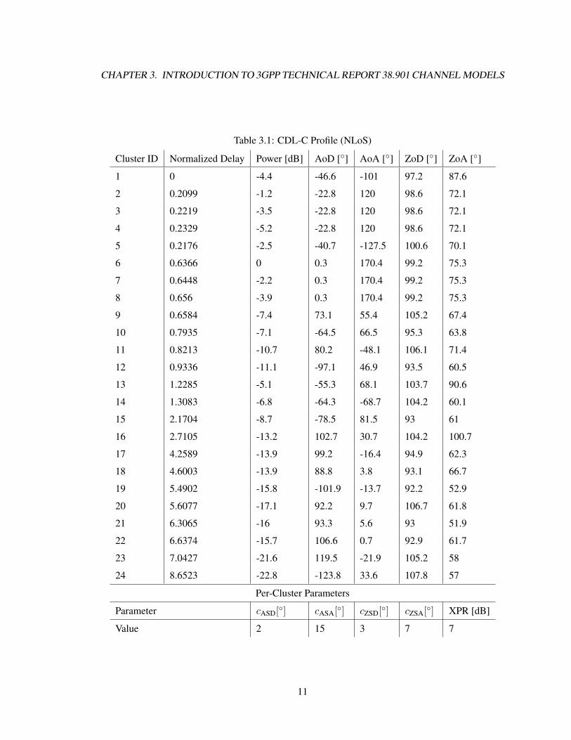
3.1.3 Set small-scale parameters, including delay spread, angular spreads, cross po-larization ratio, cluster delays, powers, arrival and departure angle

A CDL profile generally describes power, delay, angles for each clusters. As tabulated in

Table 3.1, CDL-C profile describes a LoS scenario, with 23 different clusters, and their corresponding,

• Normalized Delay, scaled by delay spread, i.e.,

τscaled = τmodel ×DSdesired (3.5)

In this simulation, we uses 16ns as the delay spread, recommended by [10] for indoor office,

normal-delay profile.

6


Figure 3.1: Pathloss vs Distance (Indoor office)

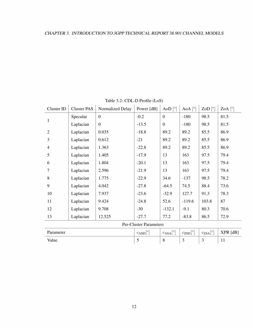
• Cluster Power, described in dB (W). Note that for LoS profiles (CDL-D, CDL-E), no scaling

of K-factor is applied, so the cluster power is directly from the Power Delay Profile (PDP).

• Azimuth angle of Arrival (AoA) φAoA, Azimuth angle of Departure (AoD) φAoD, Zenith angle

of Arrival (ZoA) θZoA, Zenith angle of Departure (ZoD) θAoD of corresponding cluster center

and cluster-wise Rooted Mean Square (RMS) angles (cASA etc.), describing how diverge within

angles of that cluster. Then these two set of parameters are used to generate paths within one

cluster by Equation 3.6

φn,m,AoA = φn,AoA + cASAαm (3.6)

where, φn,m,AoA represents path n within cluster m’s Azimuth of angle of Arrival, φn,AoA

represents the cluster center’s AoA, and cASA is the cluster-wise RMS Azimuth angle Spread of

Arrival (ASA), and αm is denotes the ray offset angles within a cluster for path m, for example,

path number 1 (m = 1), the basis vector of offset angles α1 = 0.0447, meaning the first path is

0.0447 radian deviating from the cluster center. Same logic applies for AoD-Azimuth angle

7


Spread of Depature (ASD), ZoA-Zenith angle Spread of Arrival (ZSA), ZoD-Zenith angle

Spread of Depature (ZSD).

• Cross Polarization Ratio (XPR), used to describe the power ratios for each path in each cluster

if certain cluster is of NLoS

3.1.4 Draw initial phases and generate channel coefficients

After modeling all above parameters of MultiPath Cluster (MPC), the NLoS channel of the

n-th path within cluster m ∈ [1,M ], between the u-th AP antenna and the s-th STA antenna is then

given by,

HNLoSu,s,n (t) =

√PnM

M∑m=1

FNLoSu,n,mRu,n,mTs,n,mDn,m(t) (3.7)

for LoS,

HLoSu,s,n(t) =

√PnM

M∑m=1

FLoSu,n,mRu,n,mTs,n,mDn,m(t) (3.8)

where,

• Pn is n-th path’s power

• FNLoSu,n,m stands for the field term of Equation 3.7, including receive antenna patterns Frx,u,θ and

Frx,u,φ, and transmit antenna patterns Ftx,u,θ and Ftx,u,φ, with their respects to directions of θ

and φ (the base spherical vectors) given in Global Coordinate System (GCS) [10]. Φφθn,m ,Φφφ

n,m

Φθθn,m Φθφ

n,m are random initial phases for each path m of each cluster n, κn,m = 10X/10, X is

the XPR, differs from CDL profile to profile.

FNLoSu,n,m =

Frx,u,θ(θn,m,ZoA, φn,m,AoA)

Frx,u,φ(θn,m,ZoA, φn,m,AoA)

>· exp (jΦθθ

n,m)√κ−1n,m exp (jΦθφ

n,m)√κ−1n,m exp (jΦφθ

n,m) exp (jΦφφn,m)

·

Ftx,s,θ(θn,m,ZoD, φn,m,AoD)

Ftx,s,φ(θn,m,ZoD, φn,m,AoD)

(3.9)

8


• Ru,n,m denotes receive location term, r̂rx,n,m is the spherical unit vector with arrival angles,

stated in Equation 3.10, d̄rx,u ∈ R3×1 is the location vector of receive antenna element u, and

λ0 is carrier wave length,

Ru,n,m = exp

(j2πr̂>rx,n,md̄rx,u

λ0

), r̂rx,n,m =

sin θn,m,ZoA cosφn,m,AoA

sin θn,m,ZoA sinφn,m,AoA

cos θn,m,ZoA

(3.10)

• Ts,n,m represents transmit location term, r̂rx,n,m is the spherical unit vector with departure

angles, stated in Equation 3.11, d̄tx,s ∈ R3×1 is the location vector of transmit antenna element

s,

Ts,n,m = exp

(j2πr̂>tx,n,md̄tx,s

λ0

), r̂tx,n,m =

sin θn,m,ZoD cosφn,m,AoD

sin θn,m,ZoD sinφn,m,AoD

cos θn,m,ZoD

(3.11)

• Dn,m(t) indicates the Doppler term, v̄ is the STA velocity with speed v, along azimuth angle

φv and elevation angle θv,

Dn,m(t) = exp (j2πr̂>rx,n,mv̄n,mt), v̄ = v

sin θv cosφv

sin θv sinφv

cos θv

(3.12)

• For LoS field term FLoSu,n,m, it is stated in Equation 3.13. Note that the d3D is the 3-D distance

between AP’s transmit antenna and STA’s receive antenna. The rest terms remain the same as

Equation 3.7.

FLoSu,n,m =

Frx,u,θ(θLoS, ZoA, φLoS, ZoA)

Frx,u,φ(θLoS, ZoA, φLoS, ZoA)

> ·1 0

0 −1

·Ftx,s,θ(θLoS, ZoD, φLoS, AoD)

Ftx,s,φ(θLoS, ZoD, φLoS, AoD)

· exp

(−j2πd3D

λ0

)(3.13)

9


3.1.5 Apply pathloss, shadowing and the channel coefficients to the input signal

To do so, design set of Finite Impulse Response (FIR) filters to filter input signal, apply

pathloss and shadowing afterwards. Note that the delays are read from the profile, as scaled in

Equation 3.5.

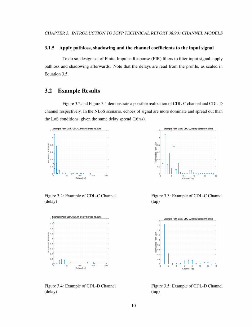
3.2 Example Results

Figure 3.2 and Figure 3.4 demonstrate a possible realization of CDL-C channel and CDL-D

channel respectively. In the NLoS scenario, echoes of signal are more dominate and spread out than

the LoS conditions, given the same delay spread (16ns).

0

0.2

0.4

0.6

0.8

1

1.2

No

rma

lize

d P

ath

Ga

in

Example Path Gain, CDL-C, Delay Spread 16.00ns

0 50 100 150 200

Delays [ns]

Figure 3.2: Example of CDL-C Channel(delay)

0

0.2

0.4

0.6

0.8

1

1.2

No

rma

lize

d P

ath

Ga

in

Example Path Gain, CDL-C, Delay Spread 16.00ns

0 5 10 15 20 25

Channel Tap

Figure 3.3: Example of CDL-C Channel(tap)

0

0.2

0.4

0.6

0.8

1

1.2

1.4

1.6

1.8

Norm

aliz

ed P

ath

Gain

Example Path Gain, CDL-D, Delay Spread 16.00ns

0 50 100 150 200

Delays [ns]

Figure 3.4: Example of CDL-D Channel(delay)

0

0.2

0.4

0.6

0.8

1

1.2

1.4

1.6

1.8

No

rma

lize

d P

ath

Ga

in

Example Path Gain, CDL-D, Delay Spread 16.00ns

0 2 4 6 8 10 12 14

Channel Tap

Figure 3.5: Example of CDL-D Channel(tap)

10


Table 3.1: CDL-C Profile (NLoS)

Cluster ID Normalized Delay Power [dB] AoD [◦] AoA [◦] ZoD [◦] ZoA [◦]

1 0 -4.4 -46.6 -101 97.2 87.6

2 0.2099 -1.2 -22.8 120 98.6 72.1

3 0.2219 -3.5 -22.8 120 98.6 72.1

4 0.2329 -5.2 -22.8 120 98.6 72.1

5 0.2176 -2.5 -40.7 -127.5 100.6 70.1

6 0.6366 0 0.3 170.4 99.2 75.3

7 0.6448 -2.2 0.3 170.4 99.2 75.3

8 0.656 -3.9 0.3 170.4 99.2 75.3

9 0.6584 -7.4 73.1 55.4 105.2 67.4

10 0.7935 -7.1 -64.5 66.5 95.3 63.8

11 0.8213 -10.7 80.2 -48.1 106.1 71.4

12 0.9336 -11.1 -97.1 46.9 93.5 60.5

13 1.2285 -5.1 -55.3 68.1 103.7 90.6

14 1.3083 -6.8 -64.3 -68.7 104.2 60.1

15 2.1704 -8.7 -78.5 81.5 93 61

16 2.7105 -13.2 102.7 30.7 104.2 100.7

17 4.2589 -13.9 99.2 -16.4 94.9 62.3

18 4.6003 -13.9 88.8 3.8 93.1 66.7

19 5.4902 -15.8 -101.9 -13.7 92.2 52.9

20 5.6077 -17.1 92.2 9.7 106.7 61.8

21 6.3065 -16 93.3 5.6 93 51.9

22 6.6374 -15.7 106.6 0.7 92.9 61.7

23 7.0427 -21.6 119.5 -21.9 105.2 58

24 8.6523 -22.8 -123.8 33.6 107.8 57

Per-Cluster Parameters

Parameter cASD[◦] cASA[◦] cZSD[◦] cZSA[◦] XPR [dB]

Value 2 15 3 7 7

11


Table 3.2: CDL-D Profile (LoS)

Cluster ID Cluster PAS Normalized Delay Power [dB] AoD [◦] AoA [◦] ZoD [◦] ZoA [◦]

1Specular 0 -0.2 0 -180 98.5 81.5

Laplacian 0 -13.5 0 -180 98.5 81.5

2 Laplacian 0.035 -18.8 89.2 89.2 85.5 86.9

3 Laplacian 0.612 -21 89.2 89.2 85.5 86.9

4 Laplacian 1.363 -22.8 89.2 89.2 85.5 86.9

5 Laplacian 1.405 -17.9 13 163 97.5 79.4

6 Laplacian 1.804 -20.1 13 163 97.5 79.4

7 Laplacian 2.596 -21.9 13 163 97.5 79.4

8 Laplacian 1.775 -22.9 34.6 -137 98.5 78.2

9 Laplacian 4.042 -27.8 -64.5 74.5 88.4 73.6

10 Laplacian 7.937 -23.6 -32.9 127.7 91.3 78.3

11 Laplacian 9.424 -24.8 52.6 -119.6 103.8 87

12 Laplacian 9.708 -30 -132.1 -9.1 80.3 70.6

13 Laplacian 12.525 -27.7 77.2 -83.8 86.5 72.9

Per-Cluster Parameters

Parameter cASD[◦] cASA[◦] cZSD[◦] cZSA[◦] XPR [dB]

Value 5 8 3 3 11

12

Chapter 4

802.11ad Receiver Reference Design and

Performance Analysis

The receiver structure mainly contains the following important components, sequentially,

4.1 DMG packet detection

The packet detector returns the offset (in time, delay per se) from the start of the input

waveform to the start of detected preamble using a simple auto-correlation, namely, that is to say,

given a received signal v(t), which is a delayed version of transmitted signal u(t) (note that this

transmitted signal is a priori, which composes Golay sequences, in STF and CEF), along with

channel (assuming static packet-wise) coefficient c and white Gaussian noise w(t), we have,

v(t) = cu(t− τ0) + w(t), t ∈ Tobs (4.1)

Under the Maximum Likelihood (ML) criterion and treating c = |c|ejθ, θ ∼ U [−π, π], we

have,

τ̂0 = arg minτ

∫Tobs

|v(t)− cu(t− τ)|2 dt

= arg maxτ<{c∗∫Tobs

v(t)u∗(t− τ)dt

}= arg max

τ

∣∣∣∣∫Tobs

v(t)u∗(t− τ)dt

∣∣∣∣(4.2)

13

CHAPTER 4. 802.11AD RECEIVER REFERENCE DESIGN AND PERFORMANCE ANALYSIS

4.2 Frequency offset estimation

It is always advantageous to separate out any frequency offset – possibly caused by relative

movement or, transceiver oscillators’ inaccuracy – in any communication system. In this frequency

offset model we have, assuming delay synchronized,

v(t) = |c|ejθ0ej2πfdtu(t) + w(t), t ∈ Tobs (4.3)

Following the same ML logic and treating c’s phase is uniformly distributed on −[π, π],

we obtain,

f̂d = arg minf

∫Tobs

∣∣∣v(t)− |c|ejθ0ej2πfdtu(t)∣∣∣2 dt

= arg maxf<{e−jθ0

∫Tobs

v(t)u∗(t)e−j2πftdt

}= arg max

f<{e−jθ0F [v(t)u∗(t)]

}= arg max

f|F [v(t)u∗(t)]|

(4.4)

where F [·] represents Fourier Transform.

4.3 Channel Estimation and Equalization

After delay and frequency synchronization, channel estimation is used for following

Frequency Domain Equalization (FDE). Because the summation of autocorrelations of Ga128 and

Gb128 composes a Dirac delta function, therefore the channel impulse response is obtained easily

by a simple correlation. Figure 4.1 shows one possible estimation results, and Figure 4.1 shows

statistical performance (in Mean Squared Error (MSE)).

4.4 Receiver state machine

A typical receiver state machine is pictured in Figure 4.4. Note that this is intended

for single carrier only, OFDM and Control PHY are not included in the figure. In the figure, red

represents PHY operations, green stands for for MAC states.

14


0 2 4 6 8 10 12 14

Channel Tap

0

0.2

0.4

0.6

0.8

1

1.2

1.4

1.6

1.8

No

rma

lize

d P

ath

Ga

in

Channel Estimation Results, SNR = 20dB, MSE = -23.33dB

Generated Channel Gains

Estimated Channel Gains

0 5 10 15 20

SNR [dB]

-18

-16

-14

-12

-10

-8

-6

MS

E [

dB

]

Channel Estimation Performance

Figure 4.1: Channel Estimation Performance

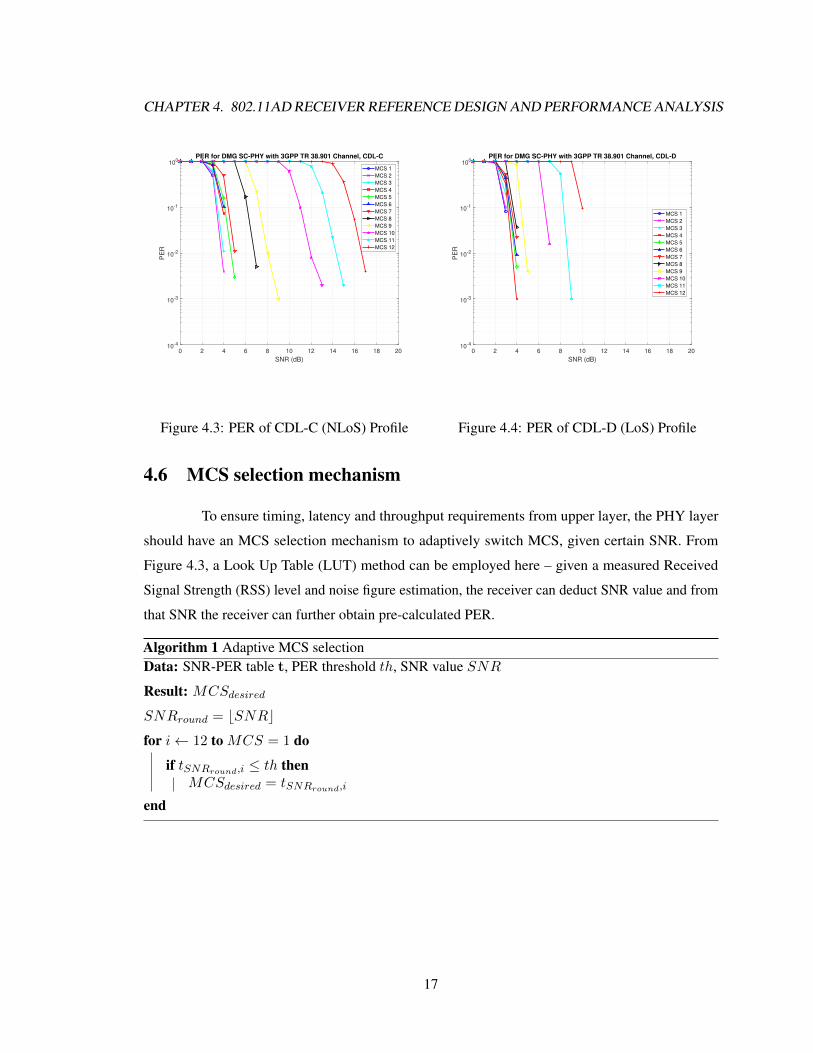
4.5 PER performance of 3GPP recommended channel

The system performance of PHY transmitter-channel-receiver structure is evaluated through

PER. The PER is defined as – a packet is successfully detected and no bit error in the payload part.

In the simulation, the parameters of channel is tabulated in Table 3.1 for CDL-C profile,

and Table 3.2 for CDL-D profile. Except from those parameters, in the 3GPP recommended channel

parameter settings, the delay spread is set to be 16 ns. System wise, according to 802.11ad protocol,

the sample rate is set to be 1760 M sa/s and the carrier frequency is set to be 60.48 GHz. Besides, no

Doppler shift is applied, i.e., the simulation scenario is static. Note that all scenarios are simulated

under 1000 packets transmission for statistical stability.

Comparing Figure 4.3 and Figure 4.4, it can be observed that CDL-C (NLoS) conditions

are worse in performance than CDL-D (LoS) conditions. For example under 10dB SNR, the PER

of MCS 12 is around 10% in CDL-D whereas 100% in CDL-C. This is because the NLoS scenario

has more MPC, as indicated in Figure 3.2, and those MPC tend to dominate (and resonate) on the

receiver side. One can also observe that with SNR rising, the SNR is decreasing because less noise

is introduced in system. Under the same SNR, lower MCS tends to be more robust than the higher

ones, which is determined by modulation method and code rate.

15


STF -- Pkt Dect., CFO Corr., Noise Est. PHY_CCA=busy

CCA/CS

SC CEF -- Chan. Est.

Detect CE Type

Y

NHeader CRC Passed?

NSupported MCS?

PHY_CCA=idle

Wait till End of Pkt.

Signal LostRx Data Field

BLK Cnt < 0

Decode/Descrable

Freq. Domain Eq., Phase Track

N

PHY_RXEND

Y

TRN Length > 0?

ProcessAGC/TRN-R

PHY_RXSTART

Figure 4.2: Receiver State Machine

16


0 2 4 6 8 10 12 14 16 18 20

SNR (dB)

10-4

10-3

10-2

10-1

100P

ER

PER for DMG SC-PHY with 3GPP TR 38.901 Channel, CDL-C

MCS 1

MCS 2

MCS 3

MCS 4

MCS 5

MCS 6

MCS 7

MCS 8

MCS 9

MCS 10

MCS 11

MCS 12

Figure 4.3: PER of CDL-C (NLoS) Profile

0 2 4 6 8 10 12 14 16 18 20

SNR (dB)

10-4

10-3

10-2

10-1

100

PE

R

PER for DMG SC-PHY with 3GPP TR 38.901 Channel, CDL-D

MCS 1

MCS 2

MCS 3

MCS 4

MCS 5

MCS 6

MCS 7

MCS 8

MCS 9

MCS 10

MCS 11

MCS 12

Figure 4.4: PER of CDL-D (LoS) Profile

4.6 MCS selection mechanism

To ensure timing, latency and throughput requirements from upper layer, the PHY layer

should have an MCS selection mechanism to adaptively switch MCS, given certain SNR. From

Figure 4.3, a Look Up Table (LUT) method can be employed here – given a measured Received

Signal Strength (RSS) level and noise figure estimation, the receiver can deduct SNR value and from

that SNR the receiver can further obtain pre-calculated PER.

Algorithm 1 Adaptive MCS selectionData: SNR-PER table t, PER threshold th, SNR value SNR

Result: MCSdesired

SNRround = bSNRcfor i← 12 to MCS = 1 do

if tSNRround,i ≤ th thenMCSdesired = tSNRround,i

end

17

Chapter 5

Introduction to Beamforming

5.1 What is beamforming?

The first attempt to automatically localize signal sources using antenna arrays was through

beamforming techniques. The idea is to steer array in one direction at a time and measure the output

power. The steering locations which result in maximum power yield the Direction of Arrival (DoA)

estimations.

The array response is steered by forming a linear combination of the sensor outputs,

y(t) =L∑l=1

w∗l xl(t) = wHx(t) (5.1)

Given samples y(1), y(2), · · · , y(N), the output power is measured by,

P (w) =1

N

N∑t=1

|y(t)|2 =1

N

N∑t=1

wHx(t)xH(t)w (5.2)

Essentially, different beamforming approaches correspond to different choices of the

weighting vector w. The weight vector applied to every antenna element can be interpreted as a

spatial filter, who equalize the delays (and perhaps attenuations as well) experienced by the signal on

various sensors to maximally combine their respective contributions.

5.2 Bartlett’s Beamformer (Conventional)

The Bartlett beamformer [11] essentially maximizes the power of the beamforming output

for a given input signal at certain direction θ. Suppose a signal measured at the array output is given

18

CHAPTER 5. INTRODUCTION TO BEAMFORMING

by,

x(t) = a(θ)s(t) + n(t) (5.3)

In Equation 5.3, s(t) is transmit signal, n(t) is spatially white noise (uncorrelated between

elements), and a(θ) is the steering vector for zenith angle θ (assuming azimuth angle φ is 0). The

steering vector will be elaborated in Section 6.1.2.

For example, L-elements Uniform Linear Array (ULA)’s steering vector is then represented

as,

aULA(θ) =[1 ejφ · · · ej(L−1)φ

]>(5.4)

where, φ = −kd cos θ = ωc d cos θ. k ∈ [0, L− 1] is the sequence number of an element,

d is the element spacing, often times λ/2. The problem of maximization of the power is then written

as,

wBF = arg maxw

E{wHx(t)xH(t)w

}= arg max

wwHE

{x(t)xH(t)

}w

= arg maxw

{E{|s(t)|2

}|wHa(θ)|2 + σ2|w|2

} (5.5)

Then if we constrain |w| = 1, the resulting solution is then,

wBF =a(θ)√

aH(θ)a(θ)(5.6)

This conventional beamformer uses every available Degree of Freedom (DoF) to concen-

trate received energy along one direction.

5.3 Capon’s Beamformer (MVDR)

Capon’s [12] method attempts basically minimize the power contributed by noise and any

signals coming from other directions than θ, while maintaining a fixed gain in the pre-specified

direction θ, distortionlessly, mathematically,

minw

P (w)

s.t.&wHa(θ) = 1(5.7)

19


where P (w) is defined in Equation 5.2. The optimum solution is then given by,

wCAP =R̂−1a(θ)

a(θ)R̂−1a(θ)(5.8)

where R̂ = 1N

∑Nt=1 x(t)xH(t). Some authors would like to use Rxx, yet the notion S

also exists. This power minimization is basically sacrificing some noise suppression capability for

more focused nulling in the directions where other sources present, i.e., reduces interference level to

un-desired directions.

5.4 Frost’s Beamformer (LCMV)

In the previous section, Capon’s beamformer simply add constraint wHa(θ) = 1, what if

we would like to have a set of constraints C, whose columns are linear independent, and correspond-

ing responses G, a single column vector, i.e. mathematically,

minw

P (w)

s.t.&CHw = G(5.9)

By using Lagrangian multipliers, optimum solution by Frost [13] can be obtained by,

wLCMV = R̂−1C[CHR̂−1C

]−1G (5.10)

In the following sub-section, several typical (special case) constraints are introduced.

5.4.1 Distortionless Constraint

In this case, one can tell that Capon’s beamformer is a subset of Frost’s beamformer, or

rather, Capon’s beamformer’s constraint wHa(θ) = 1 guarantees any signal propagate through θ

angle is distortionless.

5.4.2 Directional Constraint

The general directional constraint is,

aH(Θi)w = gi, i ∈ [0, L− 1] (5.11)

20


-100 -50 0 50 100

Azimuth Angle (degrees)

-300

-250

-200

-150

-100

-50

0

50

Norm

aliz

ed P

ow

er

(dB

)

X: -30

Y: 40

X: 45

Y: 40

X: 30

Y: -257.8X: 0

Y: -268.1

X: -60

Y: -14.13

X: 60

Y: 13.28

Figure 5.1: Normalized Power of LCMV beamformer with specified requirements

In this case, Θ can be a vector of directions (angles). Note that C ∈ CN×Mc constraint

matrix is simply composed by aH(Θi), while gi constitutes G.

For example, calculate the weights w of a 16-element ULA with,

• response of 40 dB in the direction of -30 degrees and 45 degrees azimuth,

• 0 in the direction of 0 and 30 degrees azimuth,

• and try to maintain -10 dB at direction 60 and -60 degrees.

The corresponding normalized power vs. angle plot is shown in Figure 5.1. Basically this

beamformer tries to cancel out signals from 0 and 30 degrees, and keep listening on -30 and 45

degrees while guarantees the signal power level of -60 and 60 degrees stays normal.

5.4.3 Null Constraint

This type of constraint is appropriate if there is an interfering signal (jammer) coming from

a known direction, that is to say,

aH(Θi)w, i ∈ [0, L− 1] (5.12)

21

Chapter 6

Beamforming Enabled Massive MIMO

Physical Layer Simulations

The beamforming enabled massive MIMO simulator contains the following components,

namely,

1. 802.11ad PHY transmitter – which modulate the payload, prepend STF, CEF, headers, and

append AGC, TRN-T/R fields

2. Phased array transmit processor – which contains a transmitter (transmits the input waveform

samples with specified peak power), and a radiator (converts signals into radiated waveforms

from arrays and individual sensor elements)

3. 3GPP TR 38.901 and Additive White Gaussian Noise (AWGN) channel – which impair the

signal and add noise

4. Phased array receive processor – which contains a collector (collects wave fields arriving

from specified direction into signals), and a receiver pre-amplifier (receives incoming signal,

multiplies them by amplifier gain and divides by losses)

5. 802.11ad PHY receiver – performs synchronizations, data field abstraction and demodulation

22

CHAPTER 6. BEAMFORMING ENABLED MASSIVE MIMO PHYSICAL LAYER SIMULATIONS

6.1 Phased array processors – radiators, collectors, steering vectors

6.1.1 Radiators and collectors

The radiator and the collector are dual in phased array processing. Given a symbol

vector contains U total symbols from PHY layer, say u ∈ CS×1, the radiated signal, along with

beamforming weight w ∈ CM×1 assigned individually for all M elements, is given by,

y = uwH (6.1)

(·)H represents Hermitian operation.

6.1.2 Steering Vectors

Regarding the steering vector, it is defined as,

v(x,y, z;α, φ) = exp (−j2πT(x,y, z;α, φ)) (6.2)

where T is defined in Equation 6.3. x,y, z ∈ R1×M denotes the location row vectors

(in meters) for all M antenna elements and λ defines the wavelength of antenna operating center

frequency.

T(x,y, z;α, φ) =1

λ

x

y

z

> − cos(α) cos(φ)

− cos(α) sin(φ)

− sin(α)

(6.3)

Note that α is the elevation angle of desired steering direction, α = 90◦− θ, θ is the zenith

angle. They are related to Local Coordinate System (LCS).

6.1.3 Array Response

To calculate the given array’s response at certain angle (LCS), defined in α and φ. As

illustrated in Figure 5.1, the array response operation essentially tries to read from the response plot.

r = wHv(x,y, z;α, φ) (6.4)

23


6.2 Simulator architecture

In the beamforming enabled simulator, given a potential AP-STA pair candidateSet with

total N users, their corresponding beamforming weights w, steering vector v. This simulator then

generate an output – finalSet – indicating for individual pair, the packet go through (True) or not.

Algorithm 2 Beamforming enabled 802.11ad PHY with 3GPP TR 38.901 channel model simulatorData: candidateSet, w, v

Result: finalSet

Initialization: finalSet = false

/* Generate waveforms and responses */

for i← 1 to N users doGenerate user payload, si

Generate 802.11ad PHY frame, ui

Radiate waveforms, yi = uiwi (Equation 6.1)

for j ← 1 to N users doObtain response ri,j = wH

i vj (Equation 6.4)

end

end

/* Create interference, pass through channel and receive */

for i← 1 to N users do

for j ← 1 to N users do

if j is NOT i thenyi ← yi + ri,j · yj

end

Pass yi through channel to obtain y′i

Collect waveforms to symbols u′i

Demodulate and decode user payload s′i

if s′i is si thenfinalSeti = True

end

24


PER performance of LCMV, 4 users, fixed position

16 ANT 32 ANT 64 ANT 128 ANT 144 ANT

0

0.1

0.2

0.3

0.4

0.5

0.6

0.7

0.8

0.9

1P

ER

Figure 6.1: PER of LCMV beamformer with 4users, CDL-C, fixed user position

PER performance of LCMV, 4 users, random position


0

0.1

0.2

0.3

0.4

0.5

0.6

0.7

0.8

0.9

1

PE

R

Figure 6.2: PER of LCMV beamformer with 4users, CDL-C, random user position

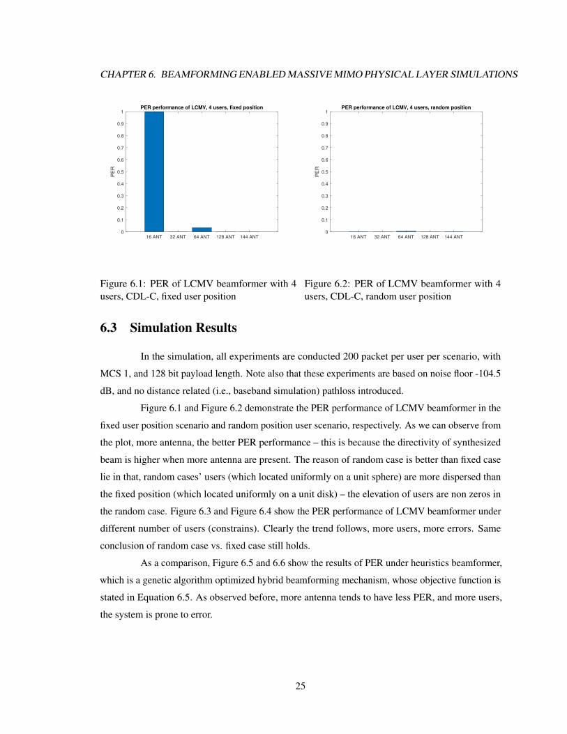
6.3 Simulation Results

In the simulation, all experiments are conducted 200 packet per user per scenario, with

MCS 1, and 128 bit payload length. Note also that these experiments are based on noise floor -104.5

dB, and no distance related (i.e., baseband simulation) pathloss introduced.

Figure 6.1 and Figure 6.2 demonstrate the PER performance of LCMV beamformer in the

fixed user position scenario and random position user scenario, respectively. As we can observe from

the plot, more antenna, the better PER performance – this is because the directivity of synthesized

beam is higher when more antenna are present. The reason of random case is better than fixed case

lie in that, random cases’ users (which located uniformly on a unit sphere) are more dispersed than

the fixed position (which located uniformly on a unit disk) – the elevation of users are non zeros in

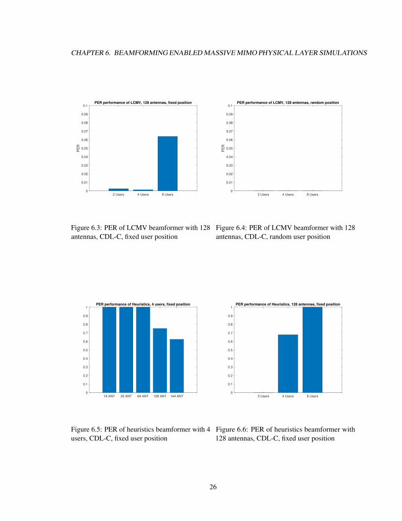
the random case. Figure 6.3 and Figure 6.4 show the PER performance of LCMV beamformer under

different number of users (constrains). Clearly the trend follows, more users, more errors. Same

conclusion of random case vs. fixed case still holds.

As a comparison, Figure 6.5 and 6.6 show the results of PER under heuristics beamformer,

which is a genetic algorithm optimized hybrid beamforming mechanism, whose objective function is

stated in Equation 6.5. As observed before, more antenna tends to have less PER, and more users,

the system is prone to error.

25


PER performance of LCMV, 128 antennas, fixed position

2 Users 4 Users 8 Users

0

0.01

0.02

0.03

0.04

0.05

0.06

0.07

0.08

0.09

0.1

PE

R

Figure 6.3: PER of LCMV beamformer with 128antennas, CDL-C, fixed user position

PER performance of LCMV, 128 antennas, random position


0

0.01

0.02

0.03

0.04

0.05

0.06

0.07

0.08

0.09

0.1

PE

R

Figure 6.4: PER of LCMV beamformer with 128antennas, CDL-C, random user position

PER performance of Heuristics, 4 users, fixed position


0

0.1

0.2

0.3

0.4

0.5

0.6

0.7

0.8

0.9

1

Figure 6.5: PER of heuristics beamformer with 4users, CDL-C, fixed user position

PER performance of Heuristics, 128 antennas, fixed position


0

0.1

0.2

0.3

0.4

0.5

0.6

0.7

0.8

0.9

1

Figure 6.6: PER of heuristics beamformer with128 antennas, CDL-C, fixed user position

26


{F∗RF,F∗BB} = arg minFRF,FBB

∑∀u∈U r̃u − ru

s.t.∑

i=j

∣∣∣F∗(i,j)RF

∣∣∣ = 1∑∀j F

∗(i,j)RF = 1, ∀i ∈ [1, NRF ]∑

i=j F∗(i,j)BB = P∑

i 6=j F∗(i,j)BB = 0

(6.5)

Note that F∗RF,F∗BB is the analog phase shifter weight and digital baseband precoder,

respectively, W = FBBFRF. r̃u is the actual throughput for user u, and ru is the desired throughput.

NRF is the number of RF chains (which is typically smaller than number of antenna in hybrid

beamforming system).

27

Chapter 7

Conclusion

With the growth of data traffic in cellular networks, and more demanding requirements,

traditional sub 6GHz system capacities are prone to reach their maximum. Millimeter wave commu-

nications are emerging recently, with its advantages in higher bandwidth and throughput, gradually

adapted in next generation of communications.

However, mmWave communication will need to overcome the exponentially growth

of pathloss caused by ten-folds on center frequency. Combining beamforming, massive MIMO

technology with mmWave communication is promising given its small wavelength. This thesis

present a massive MIMO mmWave communication link simulator design by presenting 802.11ad

PHY layer specification and its reference receiver design, along with introduction and application of

3GPP TR 38.901 channel model and beamforming enabled simulator design.

Simulation results of the proposed integrated simulator demonstrate its potential of aiding

quantification of different beamforming techniques performance through PER, a critical PHY layer

metric. Generally speaking, the simulator shows that the more antenna a system poses, the better

PER performance; whereas more user, poorer PER.

Regarding its contribution, this beamforming-communication simulator also enables the

development of MAC layer on top of PHY, by examining the validity of state machines, under

highly directional radio link which differentiate mmWave with traditional sub-6 GHz communication

protocol design – Carrier Sensing (CA) and Clear Channel Assessment (CCA) may no longer needed

or need to be revolutionized.

28

Bibliography

[1] T. S. Rappaport, S. Sun, R. Mayzus, H. Zhao, Y. Azar, K. Wang, G. N. Wong, J. K. Schulz,

M. Samimi, and F. Gutierrez, “Millimeter wave mobile communications for 5g cellular: It will

work!” IEEE access, vol. 1, pp. 335–349, 2013.

[2] W. Roh, J.-Y. Seol, J. Park, B. Lee, J. Lee, Y. Kim, J. Cho, K. Cheun, and F. Aryanfar,

“Millimeter-wave beamforming as an enabling technology for 5g cellular communications:

Theoretical feasibility and prototype results,” IEEE communications magazine, vol. 52, no. 2,

pp. 106–113, 2014.

[3] S. Sun, T. S. Rappaport, R. W. Heath, A. Nix, and S. Rangan, “Mimo for millimeter-wave

wireless communications: Beamforming, spatial multiplexing, or both?” IEEE Communications

Magazine, vol. 52, no. 12, pp. 110–121, 2014.

[4] O. El Ayach, S. Rajagopal, S. Abu-Surra, Z. Pi, and R. W. Heath, “Spatially sparse precoding

in millimeter wave mimo systems,” IEEE transactions on wireless communications, vol. 13,

no. 3, pp. 1499–1513, 2014.

[5] Z. Pi and F. Khan, “An introduction to millimeter-wave mobile broadband systems,” IEEE

communications magazine, vol. 49, no. 6, 2011.

[6] A. Natarajan, S. K. Reynolds, M.-D. Tsai, S. T. Nicolson, J.-H. C. Zhan, D. G. Kam, D. Liu,

Y.-L. O. Huang, A. Valdes-Garcia, and B. A. Floyd, “A fully-integrated 16-element phased-array

receiver in sige bicmos for 60-ghz communications,” IEEE Journal of Solid-State Circuits,

vol. 46, no. 5, pp. 1059–1075, 2011.

[7] S. Sanayei and A. Nosratinia, “Antenna selection in mimo systems,” IEEE Communications

Magazine, vol. 42, no. 10, pp. 68–73, 2004.

29

BIBLIOGRAPHY

[8] A. F. Molisch, M. Z. Win, Y.-S. Choi, and J. H. Winters, “Capacity of mimo systems with

antenna selection,” IEEE Transactions on Wireless Communications, vol. 4, no. 4, pp. 1759–

1772, 2005.

[9] “Wireless LAN Medium Access Control (MAC) and Physical Layer (PHY) Specifications

Amendment 3: Enhancements for Very High Throughput in the 60 GHz Band,” IEEE Std.

802.11ad, 2012.

[10] 3GPP, “5g; study on channel model for frequencies from 0.5 to 100 ghz,” 3rd Generation

Partnership Project (3GPP), Tech. Rep. 38.901, 2017.

[11] M. Babtlett, “Smoothing periodograms from time-series with continuous spectra,” Nature, vol.

161, no. 4096, p. 686, 1948.

[12] J. Capon, “High-resolution frequency-wavenumber spectrum analysis,” Proceedings of the

IEEE, vol. 57, no. 8, pp. 1408–1418, 1969.

[13] O. L. Frost, “An algorithm for linearly constrained adaptive array processing,” Proceedings of

the IEEE, vol. 60, no. 8, pp. 926–935, 1972.

30

Millimeter wave massive MIMO beamforming communication ...cj82ss44c/fulltext.pdfMillimeter Wave...

Documents

Transcript of Millimeter wave massive MIMO beamforming communication ...cj82ss44c/fulltext.pdfMillimeter Wave...