Eleventh Synthesis Imaging WorkshopSocorro, June 10-17, 2008

Crystal Brogan(NRAO)

Millimeter Interferometry

and ALMA

2

Outline

• The ALMA project and status

• Unique science at mm & sub-mm wavelengths

• Problems unique to mm/sub-mm observations• Atmospheric opacity• Absolute gain calibration• Tracking atmospheric phase fluctuations• Antenna and instrument constraints

• Summary

• Practical aspects of observing at high frequency with the VLA

3

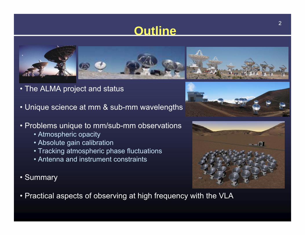
• 5000m (16,500 Ft) site in Chilean Atacama desert

• Main Array: 50 x 12m antennas (up to 64 antennas)

+ 4 x 12m (total power) + ACA: compact array of 12 x 7m antennas

• Total cost ~1.3 Billion ($US)

What is ALMA?

• A global partnership to deliver a transformational millimeter/submillimeter instrument

North America (US, Canada)Europe (ESO)East Asia (Japan,Taiwan)

ALMAAPEX

CBI

Chajnantor

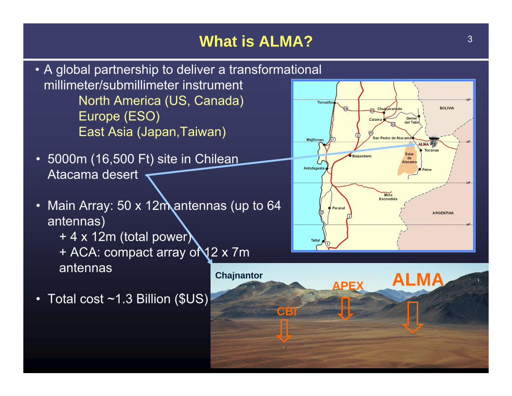
4ALMA • Baselines up to 15 km (0.015” at 300 GHz)

in “zoom lens” configurations

• A resource for ALL astronomers including pipeline products and regional science centers

• Sensitive, precision imaging between 30 to 950 GHz (10 mm to 350 µm)

• Receivers: low-noise, wide-band (8 GHz)

• Flexible correlator with high spectral resolution at wide bandwidth

• Full polarization capabilities

5

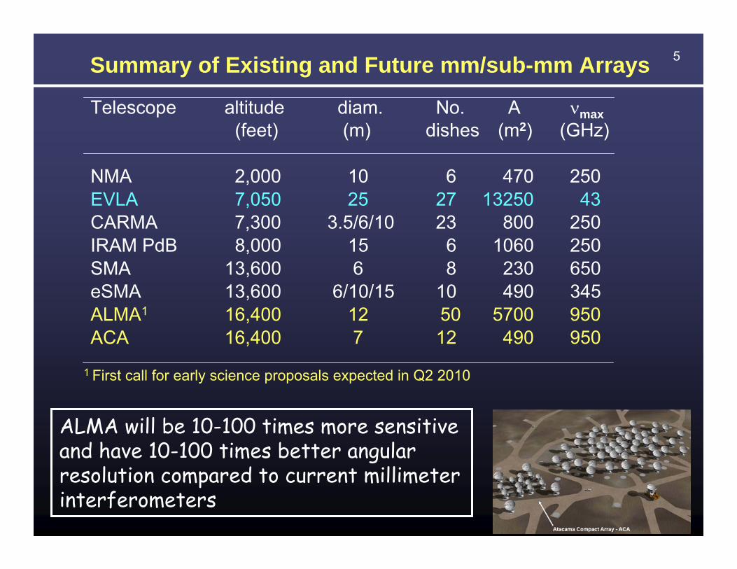
Telescope altitude diam. No. A νmax(feet) (m) dishes (m2) (GHz)

NMA 2,000 10 6 470 250EVLA 7,050 25 27 13250 43CARMA 7,300 3.5/6/10 23 800 250IRAM PdB 8,000 15 6 1060 250SMA 13,600 6 8 230 650eSMA 13,600 6/10/15 10 490 345ALMA1 16,400 12 50 5700 950ACA 16,400 7 12 490 950

Summary of Existing and Future mm/sub-mm Arrays

1 First call for early science proposals expected in Q2 2010

ALMA will be 10-100 times more sensitive and have 10-100 times better angular resolution compared to current millimeter interferometers

6

43 km to Array Operations Site (AOS)5,000m elevation 15 km to Operations Support Facility (OSF)

2,900m elevation

The Road to ALMA

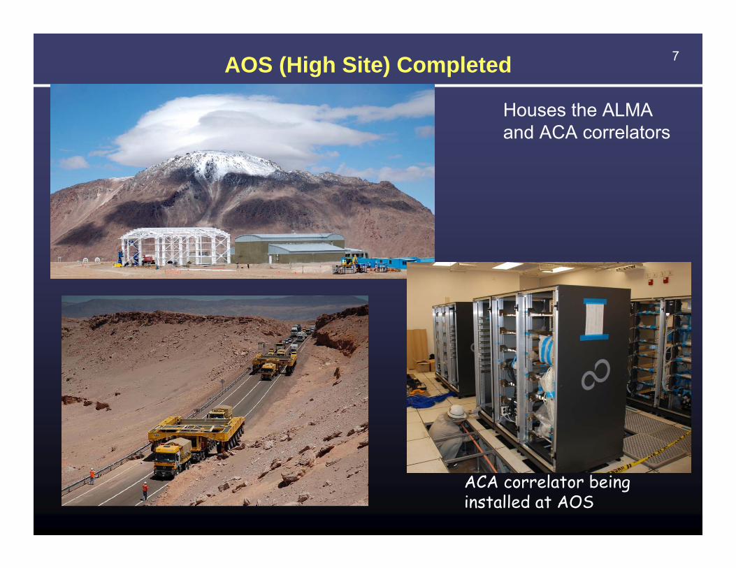
7AOS (High Site) Completed

Houses the ALMA and ACA correlators

ACA correlator being installed at AOS

8OSF (mid-level) Construction Completed

ASAC site visit Feb. 2008

AEM

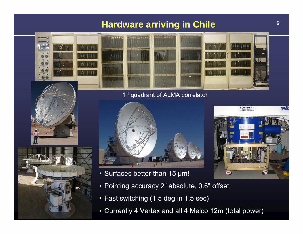
9Hardware arriving in Chile

1st quadrant of ALMA correlator

• Surfaces better than 15 µm!

• Pointing accuracy 2” absolute, 0.6” offset

• Fast switching (1.5 deg in 1.5 sec)

• Currently 4 Vertex and all 4 Melco 12m (total power)

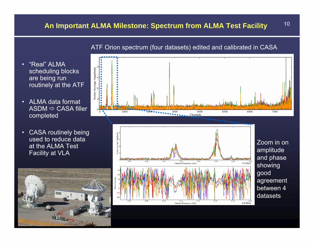
10An Important ALMA Milestone: Spectrum from ALMA Test Facility

• “Real” ALMA scheduling blocks are being run routinely at the ATF

• ALMA data format ASDM CASA filler completed

• CASA routinely being used to reduce data at the ALMA Test Facility at VLA

ATF Orion spectrum (four datasets) edited and calibrated in CASA

Zoom in on amplitude and phase showing good agreement between 4 datasets

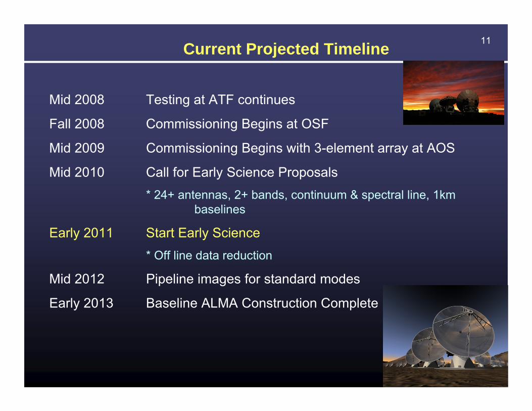
11Current Projected Timeline

Mid 2008 Testing at ATF continues

Fall 2008 Commissioning Begins at OSF

Mid 2009 Commissioning Begins with 3-element array at AOS

Mid 2010 Call for Early Science Proposals* 24+ antennas, 2+ bands, continuum & spectral line, 1km

baselines

Early 2011 Start Early Science* Off line data reduction

Mid 2012 Pipeline images for standard modes

Early 2013 Baseline ALMA Construction Complete

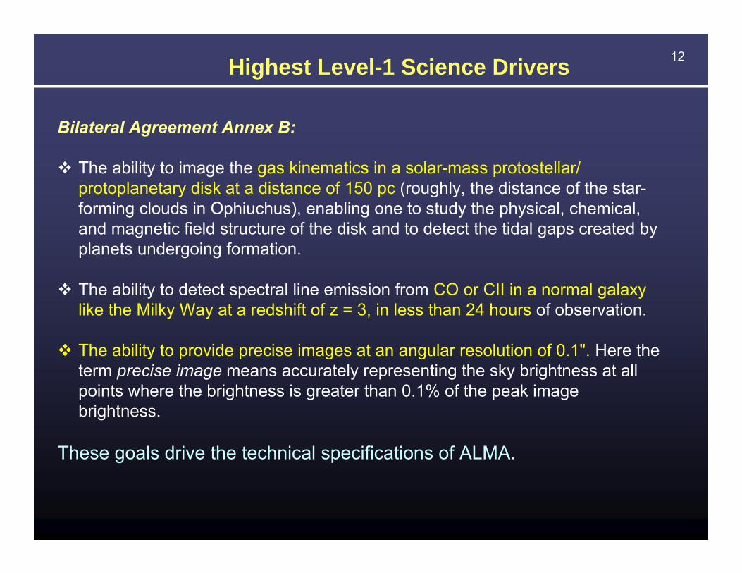
12Highest Level-1 Science Drivers

Bilateral Agreement Annex B:

The ability to image the gas kinematics in a solar-mass protostellar/ protoplanetary disk at a distance of 150 pc (roughly, the distance of the star-forming clouds in Ophiuchus), enabling one to study the physical, chemical, and magnetic field structure of the disk and to detect the tidal gaps created by planets undergoing formation.

The ability to detect spectral line emission from CO or CII in a normal galaxy like the Milky Way at a redshift of z = 3, in less than 24 hours of observation.

The ability to provide precise images at an angular resolution of 0.1". Here the term precise image means accurately representing the sky brightness at all points where the brightness is greater than 0.1% of the peak image brightness.

These goals drive the technical specifications of ALMA.

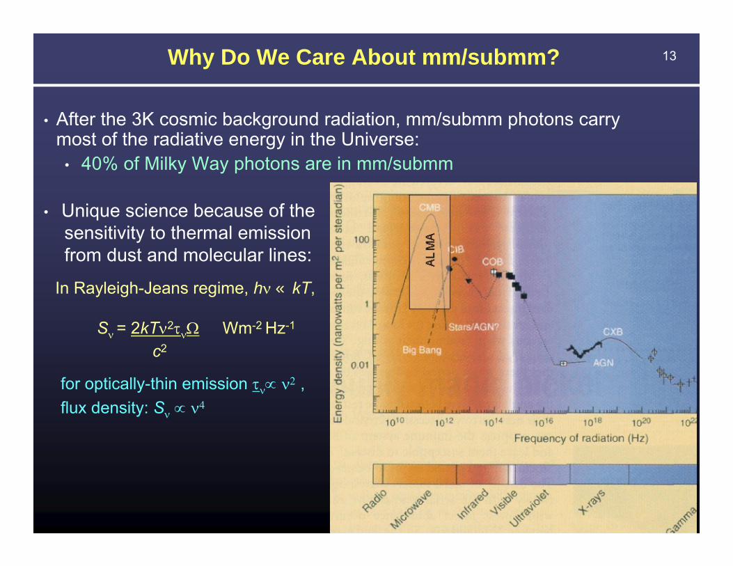
13

• After the 3K cosmic background radiation, mm/submm photons carrymost of the radiative energy in the Universe:

• 40% of Milky Way photons are in mm/submm

• Unique science because of the sensitivity to thermal emission from dust and molecular lines:

Why Do We Care About mm/submm?

In Rayleigh-Jeans regime, hν « kT,

Sν = 2kTν2τνΩ Wm-2 Hz-1

c2

for optically-thin emission τν∝ ν2 , flux density: Sν ∝ ν4

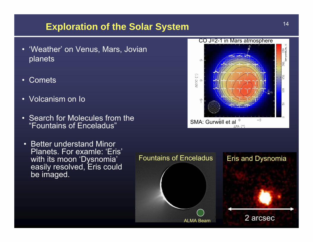
14Exploration of the Solar System

Fountains of Enceladus

ALMA Beam

Eris and Dysnomia

2 arcsec

CO J=2-1 in Mars atmosphere

SMA: Gurwell et al

• ‘Weather’ on Venus, Mars, Jovian planets

• Comets

• Volcanism on Io

• Search for Molecules from the “Fountains of Enceladus”

• Better understand Minor Planets. For examle: ‘Eris’with its moon ‘Dysnomia’easily resolved, Eris could be imaged.

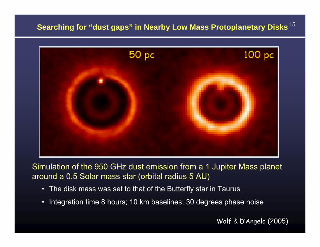
15Searching for “dust gaps” in Nearby Low Mass Protoplanetary Disks

• The disk mass was set to that of the Butterfly star in Taurus

• Integration time 8 hours; 10 km baselines; 30 degrees phase noise

Wolf & D’Angelo (2005)

Simulation of the 950 GHz dust emission from a 1 Jupiter Mass planet around a 0.5 Solar mass star (orbital radius 5 AU)

16

SMA 1.3mm continuum image of massive protocluster

NGC6334I

Understanding how Massive Stars form though Hot Core Line Emission

SMA1 SMA2

SMA3 SMA4

CO, 13CO, C17O, C18O, 34CS, SO, SO2, 34SO2, H2S, NS, SiO, H2CO, CH3OH, 13CH3OH, H13CO+

DCN, HC3N, HC5N, CH3CN, C2H5CN, NH2CH, CH3OCH3, CH3OCHO + many more + unidentified

Brogan, Hunter et al. in prep

ALMA will improve resolution and spectral line sensitivity by more than a factor of 25!

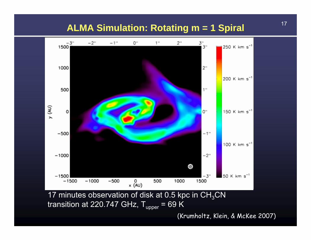
17ALMA Simulation: Rotating m = 1 Spiral

QuickTime™ and aYUV420 codec decompressor

are needed to see this picture.

17 minutes observation of disk at 0.5 kpc in CH3CN transition at 220.747 GHz, Tupper = 69 K

(Krumholtz, Klein, & McKee 2007)

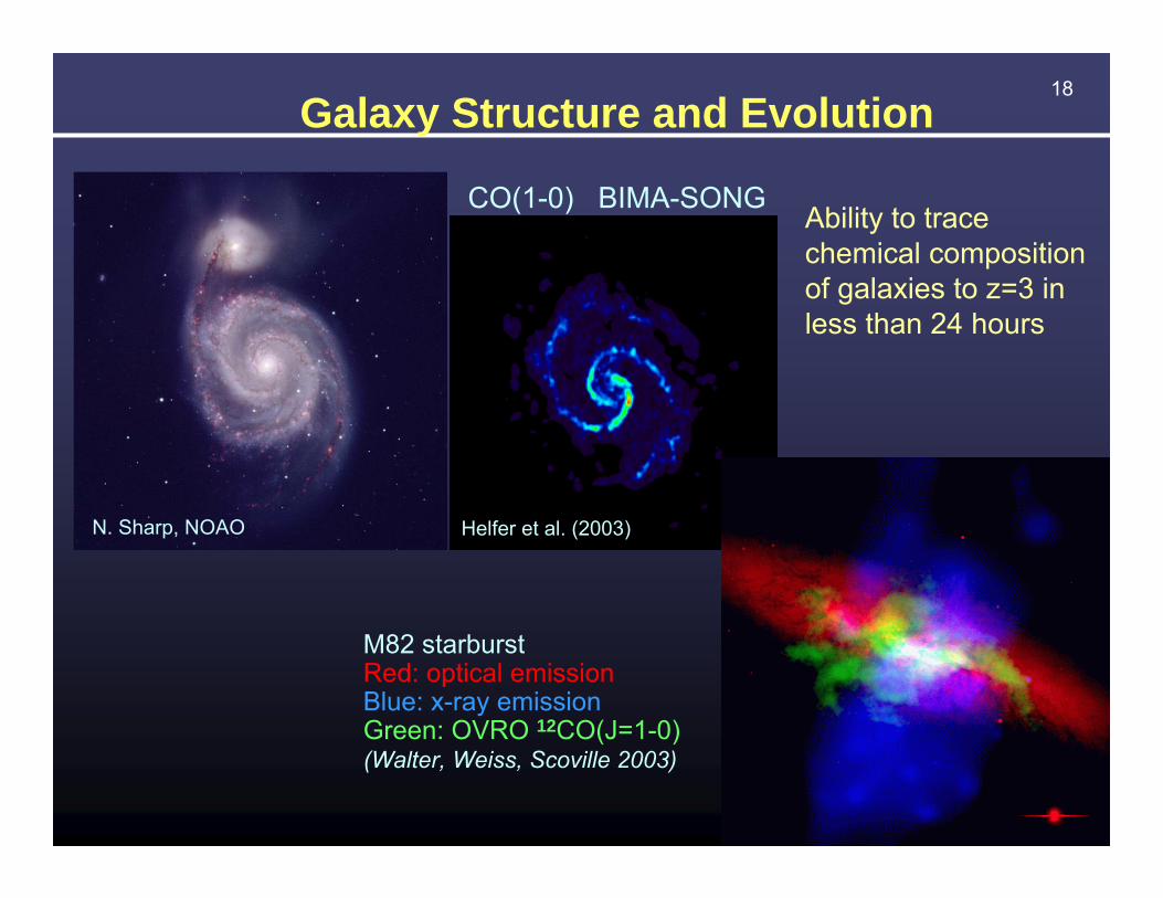
18Galaxy Structure and Evolution

N. Sharp, NOAO Helfer et al. (2003)

CO(1-0) BIMA-SONG

M82 starburstRed: optical emission Blue: x-ray emissionGreen: OVRO 12CO(J=1-0)(Walter, Weiss, Scoville 2003)

Ability to trace chemical composition of galaxies to z=3 in less than 24 hours

19Unique mm/submm access to highest z

Increasing z

Redshifting the steep submm dust SED counteracts inverse square law dimming

ALMA

Detect high-z galaxies as easily as those at z~0.5

EVLA ALMA

Spitzer

20Study of ‘first light’ During Cosmic Reionization

Current State-of-art: Tens of hours to detect rare, systems (FIR ~1x1013 L☼)

J1148+5252 z=6.42

VLA CO (3-2)

1”

Walter et al. (2004)

• Brightest submm galaxies detect dust emission in 1sec (5σ)

• Detect multiple lines in 24 hours => detailed astrochemistry

• Image dust and gas at sub-kpc resolution – gas dynamics!

HCNHCO+

CO (6-5)

CCH

94 GHz (B3)

Carilli et al. (2008)

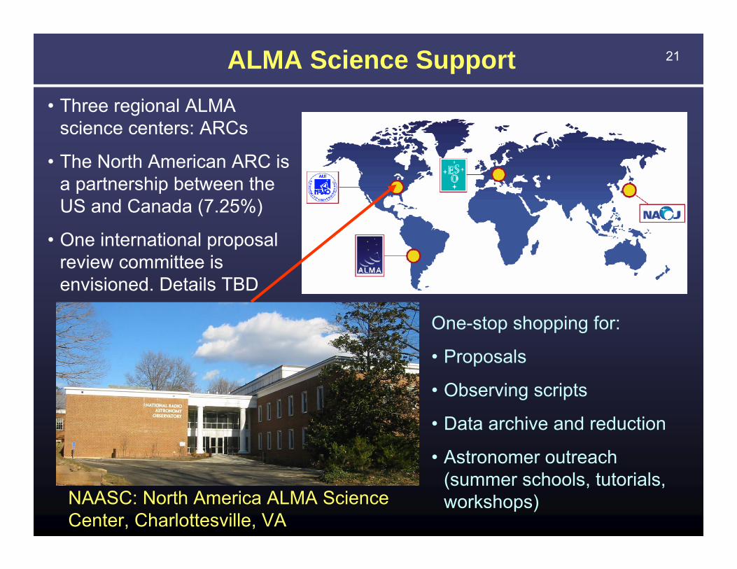
21ALMA Science Support

One-stop shopping for:

• Proposals

• Observing scripts

• Data archive and reduction

• Astronomer outreach (summer schools, tutorials, workshops)NAASC: North America ALMA Science

Center, Charlottesville, VA

• Three regional ALMA science centers: ARCs

• The North American ARC is a partnership between the US and Canada (7.25%)

• One international proposal review committee is envisioned. Details TBD

22

Problems unique to the mm/submm

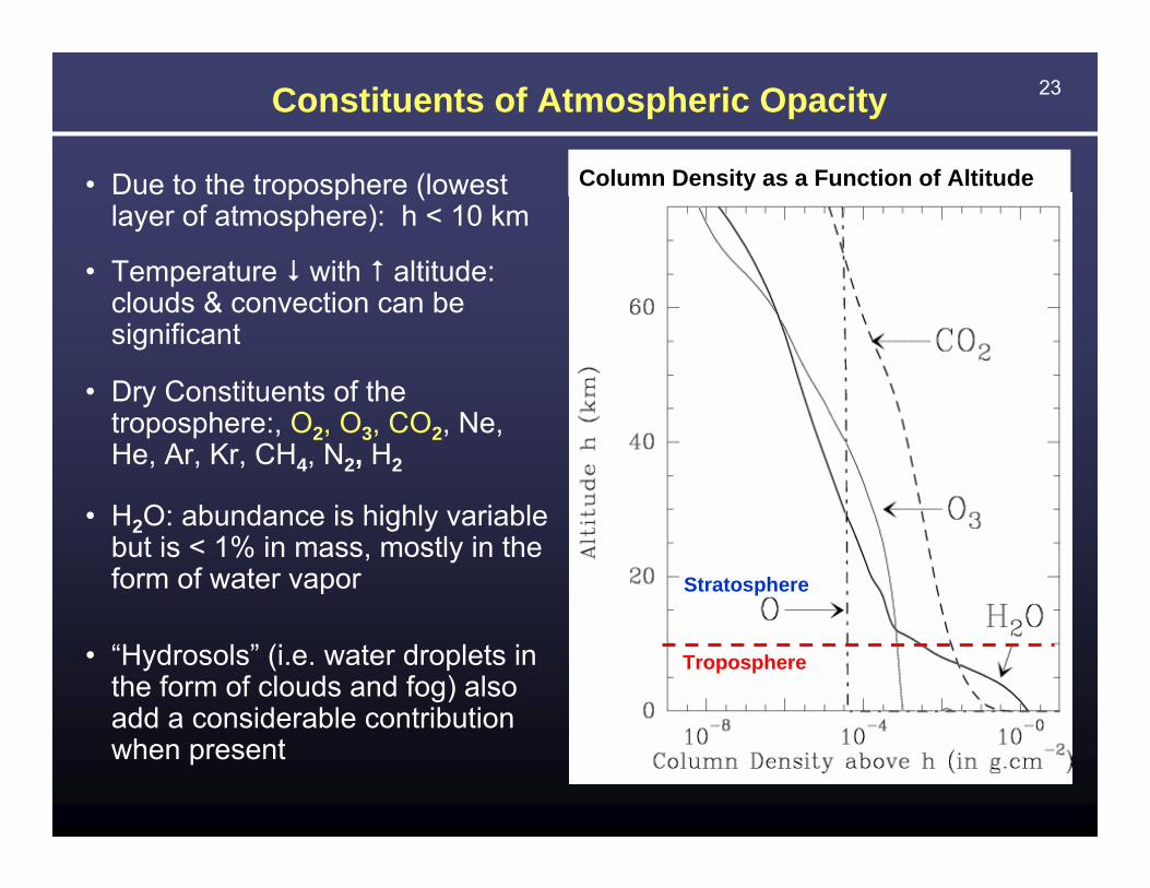
23Constituents of Atmospheric Opacity

• Due to the troposphere (lowest layer of atmosphere): h < 10 km

• Temperature with altitude: clouds & convection can be significant

• Dry Constituents of the troposphere:, O2, O3, CO2, Ne, He, Ar, Kr, CH4, N2, H2

• H2O: abundance is highly variable but is < 1% in mass, mostly in the form of water vapor

• “Hydrosols” (i.e. water droplets in the form of clouds and fog) also add a considerable contribution when present

Troposphere

Stratosphere

Column Density as a Function of Altitude

24Optical Depth as a Function of Frequency

• At 1.3cm most opacity comes from H2O vapor

• At 7mm biggest contribution from dry constituents

• At 3mm both components are significant

• “hydrosols” i.e. water droplets (not shown) can also add significantly to the opacity

43 GHz

7mm

Q band

22 GHz

1.3cm

K band

total optical depth

optical depth due to H2O vapor

optical depth due to dry air

100 GHz

3mm

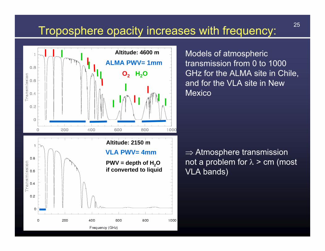
25

Models of atmospheric transmission from 0 to 1000 GHz for the ALMA site in Chile, and for the VLA site in New Mexico

⇒ Atmosphere transmission not a problem for λ > cm (most VLA bands)

PWV = depth of H2O if converted to liquid

Troposphere opacity increases with frequency:

Altitude: 2150 m

O2 H2O

Altitude: 4600 m

VLA PWV= 4mm

ALMA PWV= 1mm

26Mean Effect of Atmosphere on Phase

• Since the refractive index of the atmosphere ≠1, an electromagnetic wave propagating through it will experience a phase change (i.e. Snell’s law)

• The phase change is related to the refractive index of the air, n, and the distance traveled, D, by

φe = (2π/λ) × n × D

For water vapor n ∝ wDTatm

so φe ≈ 12.6π × w for Tatm = 270 Kλ

w=precipitable water vapor (PWV) column

This refraction causes:- Pointing off-sets, Δθ ≈ 2.5x10-4 x tan(i) (radians)

@ elevation 45o typical offset~1’

- Delay (time of arrival) off-sets

These “mean” errors are generally removed by the online system

27

In addition to receiver noise, at millimeter wavelengths the atmosphere has a significant brightness temperature (Tsky):

Sensitivity: System noise temperature

Before entering atmosphere the source signal S= Tsource

After attenuation by atmosphere the signal becomes S=Tsource e-τ

Tatm = temperature of the atmosphere ≈ 300 KTbg = 3 K cosmic background

Consider the signal-to-noise ratio: S / N = (Tsource e-τ) / Tnoise = Tsource / (Tnoise eτ)

Tsys = Tnoise eτ ≈ Tatm(eτ −1) + Trxeτ

The system sensitivity drops rapidly (exponentially) as opacity increases

For a perfect antenna, ignoring

spillover and efficiencies

Tnoise ≈ Trx + Tsky

where Tsky =Tatm (1 – e−τ) + Tbge−τ

Receiver temperature

Emission from atmosphere

so Tnoise ≈ Trx +Tatm(1-e−τ)

28Atmospheric opacity, continued

Typical optical depth for 345 GHz observing at the SMA:

at zenith τ225 = 0.08 = 1.5 mm PWV, at elevation = 30o ⇒ τ225 = 0.16

Conversion from 225 GHz to 345 GHz τ345 ≈ 0.05 + (2.25 τ225 ) ≈ 0.41

assume Tatm = 300 K and Trx=100 K

Tsys(DSB) = Tsys eτ = eτ (Tatm(1-e-τ) + Trx)= 1.5(101 + 100) ≈ 300 K

Atmosphere adds considerably to Tsys and since the opacity can change rapidly, Tsys must be measured often

Many MM/Submm receivers are double sideband, thus the effective Tsys for spectral lines (which are inherently single sideband) is doubled:

Tsys(SSB) = 2 Tsys (DSB) ~ 600 K

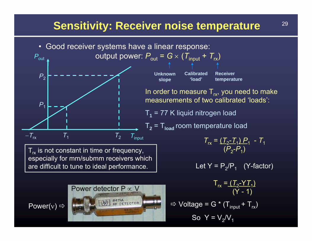
29Sensitivity: Receiver noise temperature

• Good receiver systems have a linear response: output power: Pout = G × (Tinput + Trx)Pout

TinputT1 T2

P1

P2

−Trx

Unknown slope

Calibrated ‘load’

Receiver temperature

In order to measure Trx, you need to make measurements of two calibrated ‘loads’:

T1 = 77 K liquid nitrogen load

T2 = Tload room temperature load

Trx = (T2-T1) P1 - T1 (P2-P1)

Let Y = P2/P1 (Y-factor)

Trx = (T2-YT1)(Y - 1)

Trx is not constant in time or frequency, especially for mm/submm receivers which are difficult to tune to ideal performance.

Power(ν) Voltage = G * (Tinput + Trx)

Power detector P ∝ V

So Y = V2/V1

30

• How do we measure Tsys = Tatm(eτ −1) + Trxeτ without constantly measuring Trx and the opacity?

Interferometric MM Measurement of Tsys

Power is really observed but is ∝ T in the R-J limit

Tsys = Tload * Tout / (Tin – Tout)

Vin =G Tin = [Trx + Tload]Vout = G Tout = [Trx + Tatm(1-e−τ) + Tbge−τ + Tsourcee−τ ]

SMA calibration load swings in and out of beam

Load in

Load out

• IF Tatm ≈ Tload, and Tsys is measured often, changes in mean atmospheric absorption are corrected. ALMA will have a two temperature load system which does not require assuming Tatm ≈ Tload

• Tsys is obtained by the “chopper wheel” method i.e. putting an ambient temperature load (Tload) in front of the receiver and measuring the resulting power compared to power when observing sky (Penzias & Burrus 1973).

Vin – Vout Tload

Vout Tsys=

Comparing in and out

assume Tatm ≈ Tload

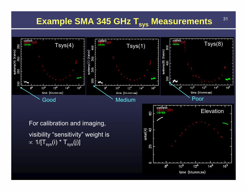
31Example SMA 345 GHz Tsys Measurements

Elevation

Tsys(4) Tsys(1) Tsys(8)

For calibration and imaging,

visibility “sensitivity” weight is ∝ 1/[Tsys(i) * Tsys(j)]

Good Medium Poor

32SMA Example of Correcting for Tsysand conversion to a Jy Scale

S = So * [Tsys(1) * Tsys(2)]0.5 * 130 Jy/K * 5 x 10-6 Jy

SMA gain for 6m dish and 75% efficiency

Correlator unit

conversion factor

Raw data Corrected data

Tsys

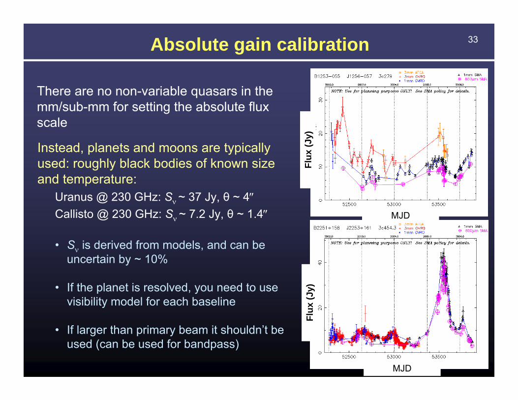
33Absolute gain calibration

There are no non-variable quasars in the mm/sub-mm for setting the absolute flux scale

Instead, planets and moons are typically used: roughly black bodies of known size and temperature:

Uranus @ 230 GHz: Sν ~ 37 Jy, θ ~ 4″Callisto @ 230 GHz: Sν ~ 7.2 Jy, θ ~ 1.4″

• Sν is derived from models, and can be uncertain by ~ 10%

• If the planet is resolved, you need to use visibility model for each baseline

• If larger than primary beam it shouldn’t be used (can be used for bandpass)

MJD

Flux

(Jy)

ΔSν= 35 Jy

ΔSν= 10 Jy

MJD

Flux

(Jy)

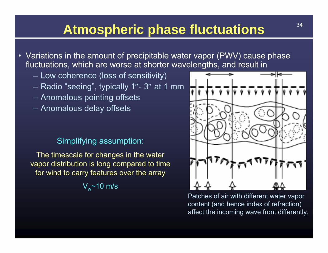
34Atmospheric phase fluctuations

• Variations in the amount of precipitable water vapor (PWV) cause phase fluctuations, which are worse at shorter wavelengths, and result in

– Low coherence (loss of sensitivity)– Radio “seeing”, typically 1″- 3″ at 1 mm– Anomalous pointing offsets– Anomalous delay offsets

Patches of air with different water vapor content (and hence index of refraction) affect the incoming wave front differently.

Simplifying assumption:The timescale for changes in the water

vapor distribution is long compared to time for wind to carry features over the array

Vw~10 m/s

35Atmospheric phase fluctuations, continued…

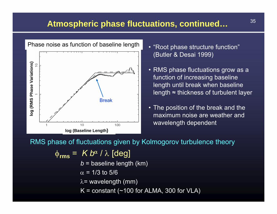
Phase noise as function of baseline length • “Root phase structure function”(Butler & Desai 1999)

• RMS phase fluctuations grow as a function of increasing baseline length until break when baseline length ≈ thickness of turbulent layer

• The position of the break and the maximum noise are weather and wavelength dependent

log

(RM

S Ph

ase

Varia

tions

)

log (Baseline Length)

Break

RMS phase of fluctuations given by Kolmogorov turbulence theory

φrms = K bα / λ [deg]b = baseline length (km)α = 1/3 to 5/6λ= wavelength (mm)K = constant (~100 for ALMA, 300 for VLA)

36Atmospheric phase fluctuations, continued…

Self-cal applied using a reference antenna within 200 m of W4 and W6, but 1000 m from W16 and W18:

Antennas 2 & 5 are adjacent, phases track each other closelyAntennas 12 &

13 are adjacent, phases track

each other closely

22 GHz VLA observations of 2 sources observed simultaneously

0423+418

0432+416

Long baselines have large amplitude, short baselines smaller amplitudeNearby antennas show correlated fluctuations, distant ones do not

37VLA observations of the calibrator 2007+404

at 22 GHz with a resolution of 0.1″ (Max baseline 30 km):

Position offsets due to large scale structures that are

correlated phase gradient

across array

one-minute snapshots at t = 0 and t = 59 min with 30min self-cal applied Sidelobe pattern

shows signature of antenna based phase errors small scale variations that are not correlated

Reduction in peak flux (decorrelation) and smearing due

to phase fluctuations over

60 min

self-cal with t = 30min:

Uncorrelated phase variations degrades and decorrelates image Correlated phase offsets = position shift

No sign of phase fluctuations with timescale ~ 30 s

self-cal with t = 30sec:

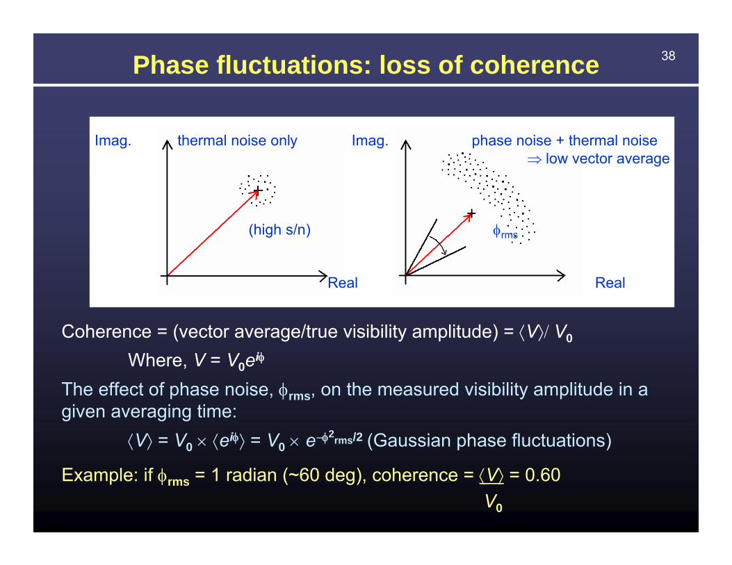
38Phase fluctuations: loss of coherence

Coherence = (vector average/true visibility amplitude) = ⟨V⟩/ V0

Where, V = V0eiφ

The effect of phase noise, φrms, on the measured visibility amplitude in a given averaging time:

⟨V⟩ = V0 × ⟨eiφ⟩ = V0 × e−φ2rms/2 (Gaussian phase fluctuations)

Example: if φrms = 1 radian (~60 deg), coherence = ⟨V⟩ = 0.60V0

Imag. thermal noise only Imag. phase noise + thermal noise⇒ low vector average

(high s/n) φrms

Real Real

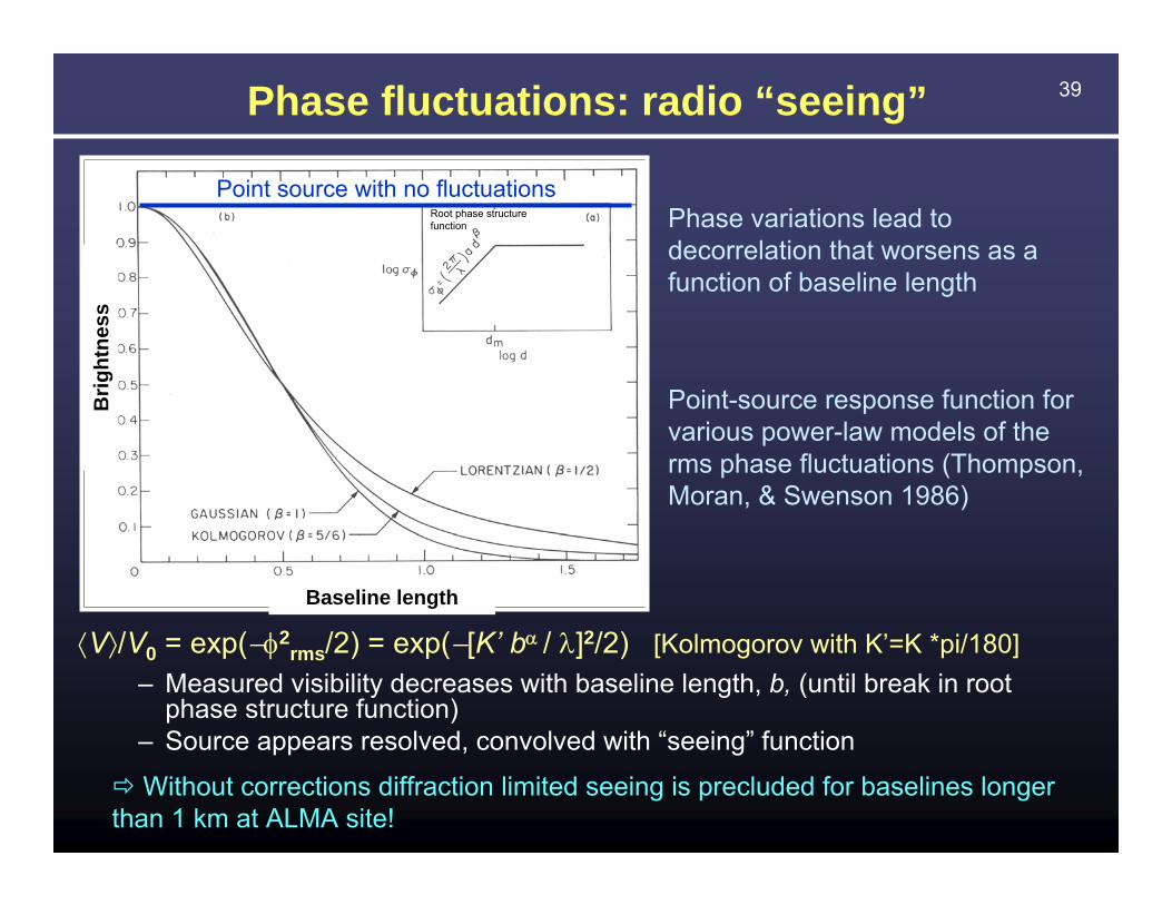
39Phase fluctuations: radio “seeing”

⟨V⟩/V0 = exp(−φ2rms/2) = exp(−[K’ bα / λ]2/2) [Kolmogorov with K’=K *pi/180]

– Measured visibility decreases with baseline length, b, (until break in root phase structure function)

– Source appears resolved, convolved with “seeing” function

Phase variations lead to decorrelation that worsens as a function of baseline length

Point-source response function for various power-law models of the rms phase fluctuations (Thompson, Moran, & Swenson 1986)

Root phase structure function

Point source with no fluctuations

Baseline length

Brig

htne

ss

Without corrections diffraction limited seeing is precluded for baselines longer than 1 km at ALMA site!

40⇒ Phase fluctuations severe at mm/submm wavelengths, correction methods are needed

• Self-calibration: OK for bright sources that can be detected in a few seconds.

• Fast switching: used at the VLA for high frequencies and will be used at CARMA and ALMA. Choose fast switching cycle time, tcyc, short enough to reduce φrms to an acceptable level. Calibrate in the normal way.

• Phase transfer: simultaneously observe low and high frequencies, and transfer scaled phase solutions from low to high frequency

• Paired array calibration: divide array into two separate arrays, one for observing the source, and another for observing a nearby calibrator.

– Will not remove fluctuations caused by electronic phase noise

– Only works for arrays with large numbers of antennas (e.g., VLA, ALMA)

41

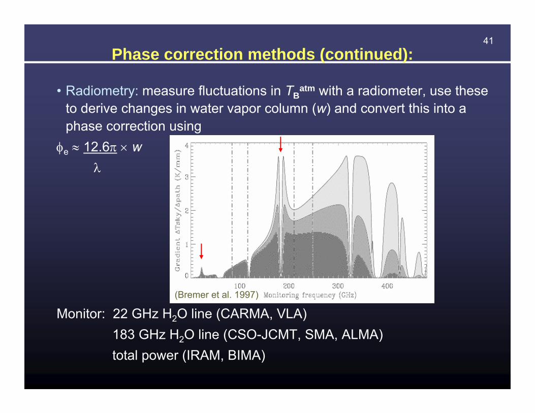
• Radiometry: measure fluctuations in TBatm with a radiometer, use these

to derive changes in water vapor column (w) and convert this into a phase correction using

φe ≈ 12.6π × wλ

Monitor: 22 GHz H2O line (CARMA, VLA)183 GHz H2O line (CSO-JCMT, SMA, ALMA)total power (IRAM, BIMA)

Phase correction methods (continued):

(Bremer et al. 1997)

42ALMA: Radiometer Phase Correction

-300

-200

-100

0

100

200

300

17:00 17:10 17:20 17:30 17:40 17:50Time (hrs:mins)

Phas

e (d

egre

es)

183 GHz Water Vapor Radiometers, tested at SMA

Mike Reid et al, 2006

Interferometer

WVR

43

• Pointing: for a 10 m antenna operating at 350 GHz the primary beam is ~ 20″

a 3″ error ⇒ Δ(Gain) at pointing center = 5%Δ(Gain) at half power point = 22%

⇒ need pointing accurate to ~1″⇒ ALMA pointing accuracy goal 0.6″

• Aperture efficiency, η: Ruze formula givesη = exp(−[4πσrms/λ]2)

⇒ for η = 80% at 350 GHz, need a surface accuracy, σrms, of 30μm⇒ ALMA surface accuracy goal of 15 µm

Antenna requirements

44Antenna requirements, continued…

• Baseline determination: phase errors due to errors in the positions of the telescopes are given by

Δφ = 2π × Δb × Δθ λ

Note: Δθ = angular separation between source and calibrator, can be > 20° in mm/sub-mm⇒ to keep Δφ < Δθ need Δb < λ/2πe.g., for λ = 1.3 mm need Δb < 0.2 mm

Δθ = angular separation between source & calibrator

Δb = baseline error

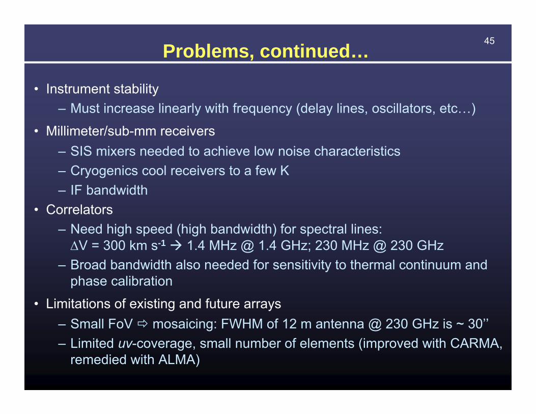
45Problems, continued…

• Instrument stability– Must increase linearly with frequency (delay lines, oscillators, etc…)

• Millimeter/sub-mm receivers– SIS mixers needed to achieve low noise characteristics– Cryogenics cool receivers to a few K– IF bandwidth

• Correlators– Need high speed (high bandwidth) for spectral lines:

ΔV = 300 km s-1 1.4 MHz @ 1.4 GHz; 230 MHz @ 230 GHz– Broad bandwidth also needed for sensitivity to thermal continuum and

phase calibration

• Limitations of existing and future arrays– Small FoV mosaicing: FWHM of 12 m antenna @ 230 GHz is ~ 30’’– Limited uv-coverage, small number of elements (improved with CARMA,

remedied with ALMA)

46Summary• ALMA construction is well underway and the science

opportunities are astounding

• Atmospheric emission can dominate the system temperature

– Calibration of Tsys is different from that at cm wavelengths

• Tropospheric water vapor causes significant phase fluctuations

– Need to calibrate more often than at cm wavelengths– Phase correction techniques are under development at all

mm/sub-mm observatories around the world– Observing strategies should include measurements to

quantify the effect of the phase fluctuations

• Instrumentation is more difficult at mm/sub-mm wavelengths

– Observing strategies must include pointing measurements to avoid loss of sensitivity

– Need to calibrate instrumental effects on timescales of 10s of mins, or more often when the temperature is changing rapidly

47

Extra Slides

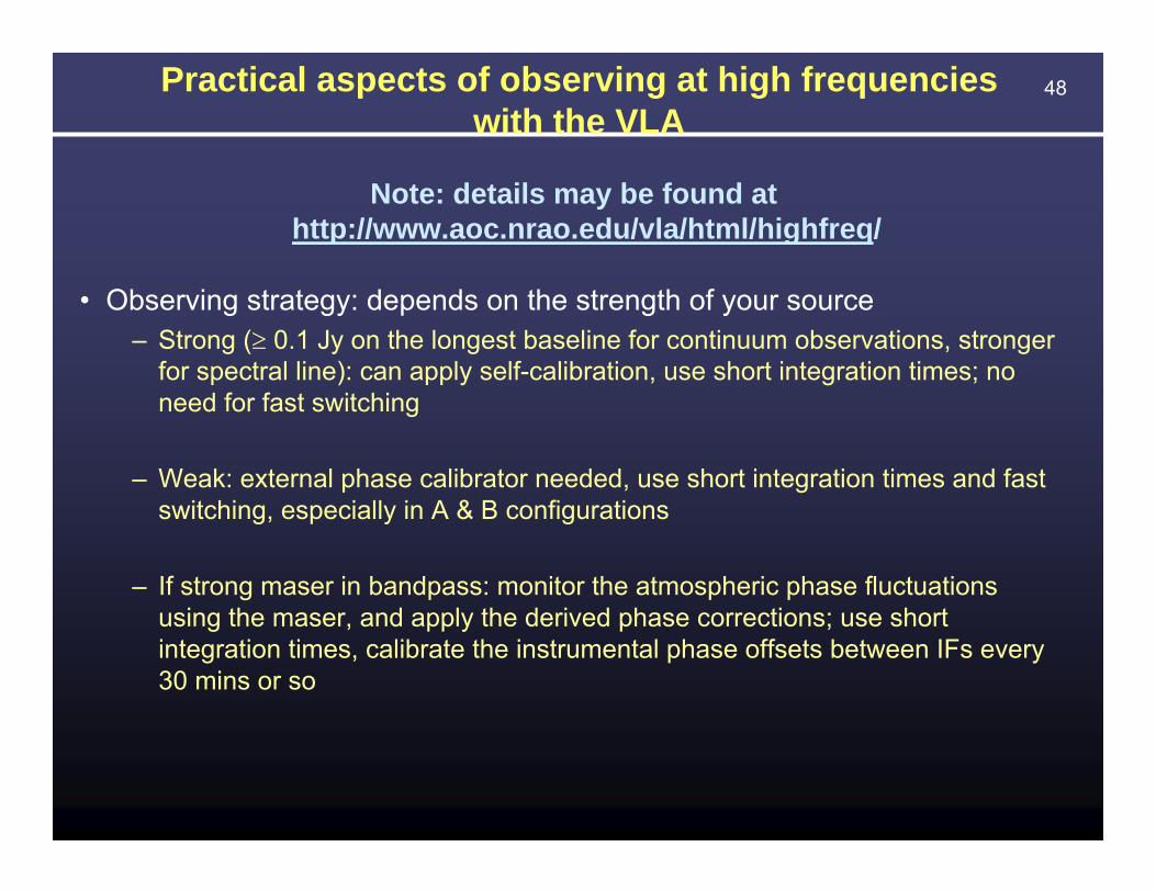
48Practical aspects of observing at high frequencies with the VLA

Note: details may be found at http://www.aoc.nrao.edu/vla/html/highfreq/

• Observing strategy: depends on the strength of your source– Strong (≥ 0.1 Jy on the longest baseline for continuum observations, stronger

for spectral line): can apply self-calibration, use short integration times; no need for fast switching

– Weak: external phase calibrator needed, use short integration times and fast switching, especially in A & B configurations

– If strong maser in bandpass: monitor the atmospheric phase fluctuations using the maser, and apply the derived phase corrections; use short integration times, calibrate the instrumental phase offsets between IFs every 30 mins or so

49Practical aspects, continued…

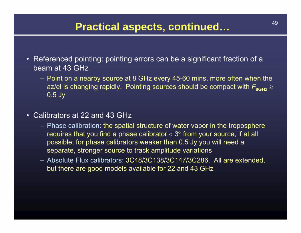
• Referenced pointing: pointing errors can be a significant fraction of a beam at 43 GHz

– Point on a nearby source at 8 GHz every 45-60 mins, more often when the az/el is changing rapidly. Pointing sources should be compact with F8GHz ≥0.5 Jy

• Calibrators at 22 and 43 GHz– Phase calibration: the spatial structure of water vapor in the troposphere

requires that you find a phase calibrator < 3° from your source, if at all possible; for phase calibrators weaker than 0.5 Jy you will need a separate, stronger source to track amplitude variations

– Absolute Flux calibrators: 3C48/3C138/3C147/3C286. All are extended, but there are good models available for 22 and 43 GHz

50Practical aspects, continued…

• If you have to use fast switching– Quantify the effects of atmospheric phase fluctuations (both

temporal and spatial) on the resolution and sensitivity of your observations by including measurements of a nearby point source with the same fast-switching settings: cycle time, distance to calibrator, strength of calibrator (weak/strong)

– If you do not include such a “check source” the temporal (but not spatial) effects can be estimated by imaging your phase calibrator using a long averaging time in the calibration

• During the data reduction– Always correct bandpass before phase and amplitude calibration– Apply phase-only gain corrections first, to avoid de-correlation of

amplitudes by the atmospheric phase fluctuations

51

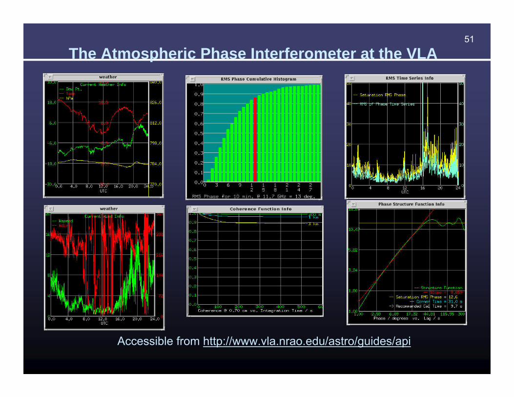
The Atmospheric Phase Interferometer at the VLA

Accessible from http://www.vla.nrao.edu/astro/guides/api

52Results from VLA 22 GHz Water Vapor Radiometry

Baseline length = 2.5 km, sky cover 50-75%, forming cumulous, n=22 GHz

Baseline length = 6 km, sky clear, n=43 GHz

Corrected Target

Uncorrected 22 GHz Target

22 GHz WVR

Corrected Target

Uncorrected 43 GHz Target

22 GHz WVR

Time (1 hour)

Phas

e (1

000

degr

ees)

Time (1 hour)

Phas

e (6

00 d

egre

es)

WVR Phase

WVR Phase

Phas

e (d

egre

es)

Phas

e (d

egre

es)

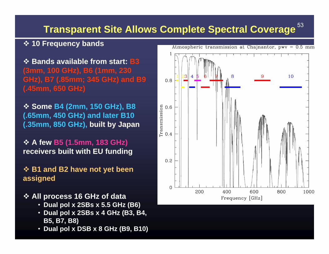
53Transparent Site Allows Complete Spectral Coverage10 Frequency bands

Bands available from start: B3 (3mm, 100 GHz), B6 (1mm, 230 GHz), B7 (.85mm; 345 GHz) and B9 (.45mm, 650 GHz)

Some B4 (2mm, 150 GHz), B8 (.65mm, 450 GHz) and later B10 (.35mm, 850 GHz), built by Japan

A few B5 (1.5mm, 183 GHz)receivers built with EU funding

B1 and B2 have not yet been assigned

All process 16 GHz of data• Dual pol x 2SBs x 5.5 GHz (B6)• Dual pol x 2SBs x 4 GHz (B3, B4,

B5, B7, B8)• Dual pol x DSB x 8 GHz (B9, B10)

54

ALMABand

Frequency Range

Receiver noise tempMixing scheme Receiver

technologyTRx over 80% of the RF band

TRx at any RF frequency

1 31.3 – 45 GHz 17 K 28 K USB HEMT2 67 – 90 GHz 30 K 50 K LSB HEMT3 84 – 116 GHz 37 K 62 K 2SB SIS4 125 – 163 GHz 51 K 85 K 2SB SIS5 163 - 211 GHz 65 K 108 K 2SB SIS6 211 – 275 GHz 83 K 138 K 2SB SIS7 275 – 373 GHz 147 K 221 K 2SB SIS8 385 – 500 GHz 98 K 147 K 2SB SIS9 602 – 720 GHz 175 K 263 K DSB SIS10 787 – 950 GHz 230 K 345 K DSB SIS

Dual, linear polarization channels:•Increased sensitivity•Measurement of 4 Stokes parameters

183 GHz water vapour radiometer:•Used for atmospheric path length correction

55

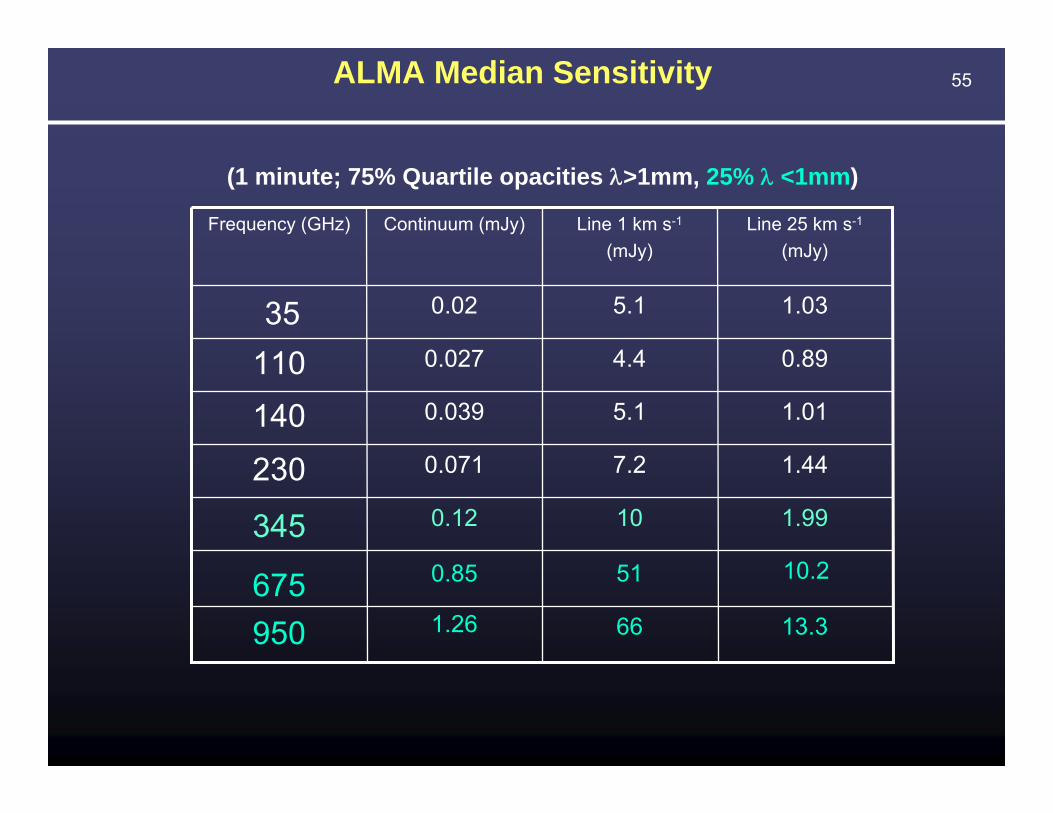
(1 minute; 75% Quartile opacities λ>1mm, 25% λ <1mm)

13.366

10.2

1.26

510.85

1.99100.12

1.447.20.071

1.015.10.039

0.894.40.027

1.035.10.0235110 140

230

345

675950

Line 25 km s-1

(mJy)Line 1 km s-1

(mJy)Continuum (mJy)Frequency (GHz)

ALMA Median Sensitivity