MNRAS 463, 2768–2780 (2016) doi:10.1093/mnras/stw2098Advance Access publication 2016 August 20

Milankovitch cycles of terrestrial planets in binary star systems

Duncan Forgan‹

Scottish Universities Physics Alliance (SUPA), School of Physics and Astronomy, University of St Andrews, North Haugh KY16 9SS, UK

Accepted 2016 August 18. Received 2016 August 17; in original form 2016 July 6

ABSTRACTThe habitability of planets in binary star systems depends not only on the radiation environmentcreated by the two stars, but also on the perturbations to planetary orbits and rotation producedby the gravitational field of the binary and neighbouring planets. Habitable planets in binariesmay therefore experience significant perturbations in orbit and spin. The direct effects of orbitalresonances and secular evolution on the climate of binary planets remain largely unconsidered.We present latitudinal energy balance modelling of exoplanet climates with direct couplingto an N-Body integrator and an obliquity evolution model. This allows us to simultaneouslyinvestigate the thermal and dynamical evolution of planets orbiting binary stars, and discovergravito-climatic oscillations on dynamical and secular time-scales. We investigate the Kepler-47 and Alpha Centauri systems as archetypes of P- and S-type binary systems, respectively.In the first case, Earth-like planets would experience rapid Milankovitch cycles (of order1000 yr) in eccentricity, obliquity and precession, inducing temperature oscillations of similarperiods (modulated by other planets in the system). These secular temperature variations haveamplitudes similar to those induced on the much shorter time-scale of the binary period. Inthe Alpha Centauri system, the influence of the secondary produces eccentricity variations on15 000 yr time-scales. This produces climate oscillations of similar strength to the variation onthe orbital time-scale of the binary. Phase drifts between eccentricity and obliquity oscillationscreates further cycles that are of order 100 000 yr in duration, which are further modulated byneighbouring planets.

Key words: astrobiology – methods: numerical – planets and satellites: general.

1 IN T RO D U C T I O N

Approximately half of all solar type stars reside in binary systems(Duquennoy & Mayor 1991; Raghavan et al. 2010). Recent exo-planet detections have shown that planet formation in these systemsis possible. Planets can orbit one of the stars in the so-called S-typeconfiguration, such as γ Cephei (Hatzes et al. 2003), HD41004b(Zucker et al. 2004), and GJ86b (Queloz et al. 2000). If the binarysemimajor axis is sufficiently small, then the planet can orbit thesystem centre of mass in the circumbinary or P-type configuration.Planets in this configuration were first detected around post-main-sequence stars, in particular the binary pulsar B160-26 (Thorsett,Arzoumanian & Taylor 1993; Sigurdsson et al. 2003). The Keplerspace telescope has been pivotal in detecting circumbinary planetsorbiting main-sequence stars, such as Kepler-16 (Doyle et al. 2011),Kepler-34 and Kepler-35 (Welsh et al. 2012), and Kepler-47 (Oroszet al. 2012).

Planets in binary systems are sufficiently common that we shouldconsider their habitability seriously. As of 2016 July, 112 exoplanets

� E-mail: dhf3@st-andrews.ac.uk

have been detected in binary star systems,1 giving an occurrencerate of around 4 per cent [previous estimates on a much smallerexoplanet population by Desidera & Barbieri (2007) placed thefraction of planets in S-type systems at 20 per cent]. At gas giantmasses, the occurrence rate of planets around P-type binaries isthought to be similar to that of single stars (Armstrong et al. 2014a).

However, theoretical modelling indicates that the dynamical land-scape of the binary significantly affects the planet formation pro-cess, both for S-type (Wiegert & Holman 1997; Quintana et al.2002, 2007; Thebault, Marzari & Scholl 2008, 2009; Xie, Zhou &Ge 2010; Rafikov & Silsbee 2014b,a) and P-type systems (Doolin& Blundell 2011; Dunhill & Alexander 2013; Martin, Armitage& Alexander 2013; Marzari et al. 2013; Rafikov 2013; Meschiari2014; Silsbee & Rafikov 2015). Therefore, when considering theprospects for habitable worlds in the Milky Way, one must take careto consider the effects that companion stars will have on the thermaland gravitational evolution of planets and moons.

The habitable zone (HZ) concept (Huang 1959; Hart 1979) isoften employed to determine whether a detected exoplanet might

1 http://www.univie.ac.at/adg/schwarz/multiple.html

C© 2016 The AuthorPublished by Oxford University Press on behalf of the Royal Astronomical Society

Milankovitch cycles in binary systems 2769

be expected to be conducive to surface liquid water (that is, if itsmass and atmospheric composition allow it). Initially calculated forthe single star case using 1D radiative transfer modelling of thelayers of an Earth-like atmosphere (Kasting, Whitmire & Reynolds1993), this quickly establishes a range of orbital distances that pro-duce clement planetary conditions. Over time, line radiative transfermodels have been refined, leading to improved estimates of the innerand outer HZ edges (Kopparapu et al. 2013, 2014).

In the case of multiple star systems, the presence and motion ofextra sources of gravity and radiation have following two importanteffects:

(i) the morphology and location of the system’s HZ changes withtime, and

(ii) regions of the system are orbitally unstable.

These joint thermal–dynamical constraints on habitability have beenaddressed in a largely decoupled fashion using a variety of analyticaland numerical techniques.

The thermal time dependence of the HZ can be evaluated bycombining the flux from both stars, taking care to weight eachcontribution appropriately, and applying the single star constraintsto determine whether a particular spatial location would receiveflux conducive to surface water. Kane & Hinkel (2013) use theaggregate flux to find a peak wavelength of emission. Assuming thecombined spectrum resembles a blackbody, Wien’s Law providesan effective temperature for the total insolation, and hence the limitsof Kopparapu et al. (2013) can be applied. This approximation isacceptable for P-type systems, where the distance from each star tothe planet is similar.

Haghighipour & Kaltenegger (2013) and Kaltenegger &Haghighipour (2013) weight each star’s flux by its effective tem-perature, and then determine the regions at which this weighted fluxmatches that of a 1 M� star at the HZ boundaries. This approach issuitable for both S-type and P-type systems. A detailed analytic so-lution for calculations of this nature has been undertaken by Cuntz(2014).

Mason et al. (2013) take a similar approach, but they also notethat for P-type systems, the tidal interaction between primary andsecondary can induce rotational synchronization, which can reduceextreme UV flux and stellar wind pressure, improving conditions inthe HZ compared to the single star case [see also Zuluaga, Mason& Cuartas-Restrepo (2016)].

The dynamical constraints on habitability rely heavily on N-Bodysimulation, most prominently the work of Dvorak (Dvorak 1984,1986) and Holman & Wiegert (1999). By integrating an ensem-ble of test particles in a variety of orbits around a binary, regionsof dynamical instability can be determined. Holman & Wiegert(1999) used these simulations to develop empirical expressions fora critical orbital semimajor axis, ac. In the case of a P-type system,this represents a minimum value – anything inside ac is orbitallyunstable, as given by the following expression:

ap > ac = abin ((1.6 ± 0.04) + (5.1 ± 0.05)ebin

+(4.12 ± 0.09)μ − (2.22 ± 0.11)e2bin − (4.27 ± 0.17)μebin

−(5.09 ± 0.11)μ2 + (4.61 ± 0.36)μ2e2bin

). (1)

In the case of an S-type system, ac represents a maximum value:

ap < ac = abin ((0.464 ± 0.006) − (0.38 ± 0.01)μ

−(0.631 ± 0.034)ebin + (0.586 ± 0.061)μebin

+(0.15 ± 0.041)e2bin − (0.198 ± 0.074)μe2

bin

), (2)

where abin is the binary semimajor axis, ebin is the binary orbitaleccentricity, and μ represents the binary mass ratio:

μ = M2

M1 + M2. (3)

The majority of binary habitability calculations rely on the above dy-namical constraints. Notable exceptions include Eggl et al. (2012)’suse of Fast Lyapunov Indicators for chaos detection, which yieldslightly smaller values of ac for S-type systems (Pilat-Lohinger &Dvorak 2002), and Jaime, Aguilar & Pichardo (2014)’s use of in-variant loops to discover non-intersecting orbits (Pichardo, Sparke& Aguilar 2005). There is a good deal of research into spin–orbitalignments of extrasolar planets under the influence of inclined stel-lar companions (e.g. Anderson, Storch & Lai 2016), but this workrarely pertains to terrestrial planet habitability. On the other hand,the evolution of planetary rotation period has been studied intentlywith regards to habitability of planets in single star systems (e.g.Bolmont et al. 2014; Brown et al. 2014; Cuartas-Restrepo et al.2016).

All the above approaches to determining habitability in binarysystems rely on an initial 1D calculation of the atmosphere’s re-sponse to radiative flux, where the key dimension is atmosphericdepth. Equally, 1D approaches can consider the latitudinal variationof flux on a planet’s surface, giving rise to the so-called latitudi-nal energy balance models or LEBMs, which have been used bothin the single star case (Spiegel, Menou & Scharf 2008; Dressinget al. 2010; Vladilo et al. 2013) and for multiple stars (Forgan 2012,2014). These are better suited to capture processes that depend onatmospheric circulation, such as the snowball effect arising fromice-albedo feedback (Pierrehumbert 2005; Tajika 2008), which islikely to occur in systems where the orbits undergo Milankovitchcycles and other secular evolution (Spiegel et al. 2010).

However, all these approaches typically decouple the thermalfrom the dynamical. The orbital constraints on the HZ are consid-ered separately from the radiative transfer calculations. While theyare eventually combined, the binary HZs that are constructed do notincorporate the effects of coupled gravito-thermal perturbations. In-deed, Holman & Wiegert (1999) admit that their empirical limits onsemimajor axis ignore the potential for stable resonances inside theinstability region, as well as unstable resonances in stable regions(cf. Chavez et al. 2014). It is likely that planets on stable orbitsin binary systems will experience relatively strong orbital elementevolution. For example, circumbinary planets can undergo rapidprecession of periapsis, which affects their ability to be detected viatransit (Kostov et al. 2014; Welsh et al. 2015). Presumably the spinevolution of planets in this situation can proceed with similar rapid-ity. Crucially, climate systems are nonlinear, and can alter their stateon very short time-scales compared to the planet’s orbital period.

In this work, we consider coupled gravito-thermal perturbationson the climate of exoplanets in binary systems. To do so, we presenta LEBM directly coupled to an N-Body integrator and an obliq-uity evolution model. We use this combined code to investigate thespin–orbital-climate dynamics of putative planets in two archetypalbinary systems: the P-type system Kepler-47, a multiplanet cir-cumbinary system which possesses one exoplanet inside the HZ(Orosz et al. 2012); and Alpha Centauri, the nearest star system tothe Sun, an S-type binary system which was thought to possess ashort period, Earth-mass exoplanet (Dumusque et al. 2012).2 By

2 This detection is no longer considered to be credible by some groups,due to concerns with how stellar activity is filtered out of radial velocity

MNRAS 463, 2768–2780 (2016)

2770 D. Forgan

evolving the orbits of the bodies in tandem with the climate, weare able to detect climate variations that are directly linked to thebinary’s orbit, and the secular evolution of the planet’s orbit andspin.

In Section 2, we describe the LEBM, and how the N-Body modelis coupled to it. In Section 3, we describe the simulation setupand results on dynamical and secular time-scales, in Section 4,we discuss the implications for habitability, and in Section 5, wesummarize the work.

2 M E T H O D

2.1 Latitudinal energy balance modelling

Typically, LEBMs solve the following diffusion equation:

C∂T (x, t)

∂t− ∂

∂x

(D(1 − x2)

∂T (x, t)

∂x

)= S(1 − A(T )) − I (T ).

(4)

Where T(x, t) is the surface temperature, C is the effective heatcapacity of the atmosphere, S is the insolation flux, I is the IRcooling and A is the albedo. In the above equation, C, S, I and A arefunctions of x (either explicitly, as S is, or implicitly through T). Thelatitude λ appears through x ≡ sin λ. This equation is evolved withthe boundary condition dT

dx= 0 at the poles (where λ = [−90, 90]◦),

and requires the assumption that the planet rotates rapidly relativeto its orbital period. Our implementation of the LEBM follows thatof Spiegel et al. (2008), and has been used previously in studyingthe climate evolution of planets in binary systems on time-scales oforder a few hundred years (Forgan 2012, 2014). In our approach, weconsider a given latitude to be habitable if its temperature resideswithin 273 K < T < 373 K, i.e. that surface water is liquid.

The diffusion coefficient D determines the efficiency of heatredistribution across latitudes. Its value is defined such that a fiducialEarth-like planet, rotating with period 1 d, orbiting at 1 au around astar of 1 M�, produces the correct average temperature profile (seee.g. Spiegel et al. 2008; Vladilo et al. 2013). If the planet’s rotation ismore rapid, the Coriolis effect will inhibit latitudinal heat transport(see Farrell 1990):

D = 5.394 × 102

(�rot

�rot,⊕

)−2

, (5)

where �rot is the rotational angular velocity of the planet, and �rot,⊕is the rotational angular velocity of the Earth. This is a necessarilysimple expression, but can be made more rigorous through includ-ing terms for atmospheric pressure and mean molecular weight(e.g. Williams & Kasting 1997, but see also Vladilo et al. 2013’sattempts to introduce a latitudinal dependence to D to mimic theHadley convective cells on Earth). Beyond this, full global circu-lation modelling is needed to explore the effects of rotation (DelGenio 1993, 1996).

As in previous work, we solve equation (4) using an explicitforward time, centre space finite difference algorithm. A globaltimestep is used, with standard constraint

�tLEBM <(�x)2 C

2D(1 − x2). (6)

data (Hatzes 2013). Recent attempts to detect α Cen Bb via transit show anull result (Demory et al. 2015), and re-analysis of the radial velocity datasuggests that α Cen Bb does not exist (Rajpaul, Aigrain & Roberts 2016).

The atmospheric heat capacity C, is a function of the planet’s surfaceocean fraction and how much of that is frozen, fice:

C = flandCland + focean ((1 − fice)Cocean + ficeCice) , (7)

where fland = 1 − focean. The heat capacities of land, ocean and icecovered areas are

Cland = 5.25 × 109erg cm−2 K−1

Cocean = 40.0Cland

Cice =⎧⎨⎩

9.2Cland 263 K < T < 273 K

2Cland T < 263 K.

The infrared cooling function I is

I (T ) = σSBT 4

1 + 0.75τIR(T ), (8)

with the optical depth of the atmosphere given as

τIR(T ) = 0.79

(T

273 K

)3

. (9)

The albedo function is

A(T ) = 0.525 − 0.245 tanh

[T − 268 K

5 K

]. (10)

This correctly reproduces the ice-albedo feedback phenomenon,which allows a rapid nonlinear increase in albedo as the ice coverageincreases.

At any instant, for a single star, the insolation received at a givenlatitude at an orbital distance r is

S = q0 cos Z

(1 au

r

)2

, (11)

where q0 is the bolometric flux received from the star at a distanceof 1 au, and Z is the zenith angle:

q0 = 1.36 × 106

(M

M�

)4

erg s−1cm−2 (12)

cos Z = μ = sin λ sin δ + cos λ cos δ cos h. (13)

The solar hour angle is h, and δ is the solar declination, which iscalculated by computing the scalar product of the spin-axis vectors and the planet–star separation vector r . We obtain the spin-axisvector by rotation of the angular momentum vector in the x-axis byδ0, followed by a rotation around the axis defined by the angularmomentum vector by pa, the axial precession angle (or longitudeof winter solstice).

Our rapid rotation assumption requires that we use diurnallyaveraged quantities, so we also diurnally average S:

S = q0μ. (14)

We do this by integrating μ over the sunlit part of the day, i.e. h= [−H, +H], where H(x) is the radian half-day length at a givenlatitude. Multiplying by H/π (as H = π if a latitude is illuminatedfor a full rotation) gives the total diurnal insolation as

S = q0

(H

π

)μ = q0

π(H sin λ sin δ + cos λ cos δ sin H ) . (15)

The radian half-day length is calculated as

cos H = − tan λ tan δ. (16)

MNRAS 463, 2768–2780 (2016)

Milankovitch cycles in binary systems 2771

The total insolation is a simple linear combination of the contribu-tions from both stars. If one star is eclipsed by the other, then weset its contribution to S to zero. We ensure that the simulation canaccurately model an eclipse by adding an extra timestep criterion,ensuring that the transit’s duration will not be less than 10 timesteps.

We fix the parameters of the model to those of the Earth: theinitial obliquity is set to 23.5◦, and the ocean fraction focean = 0.7.The rotation period of the body is 1 d. It is important to note thataltering these parameters will alter the strength of climate fluc-tuations, especially if orbits are eccentric. Indeed, Forgan (2012)showed that reducing the planet’s ocean fraction can significantlyboost temperature fluctuations in S-type binary systems with fixedorbits, and that increasing obliquity while holding other parametersfixed typically increases the average temperature of the planet. Thefollowing results should be considered with these facts in mind.

2.2 The N-Body model

The dynamical evolution of the system utilizes a standard fourth-order Hermite integrator with an adaptive shared timestep. We cal-culate this N-Body timestep for all bodies{i}, �tN, by finding theminimum value of �ti:

�ti =(

η

ai

ji+ ji

sici

si+ si

ji

)1/2

. (17)

Here, a represents the magnitude of the body’s acceleration, ji si andci are the magnitudes of the first, second and third derivatives of theacceleration of particle i, respectively, and η is a tunable parameterwhich we set to 0.002. This is a fairly strict timestep condition, andas such the error in angular momentum is typically one in 106 orbetter throughout.

2.3 Obliquity evolution

We adopt the obliquity evolution model of Laskar (1986a,b), de-veloped for the Solar system and subsequently used for putativeexoplanet systems (Armstrong, Leovy & Quinn 2004; Armstronget al. 2014b). In this paradigm, the evolution of the obliquity δ0 andprecession pa are functions of the inclination variables

p = sin

(i

2

)sin � (18)

q = sin

(i

2

)cos �. (19)

Where i is the inclination, and � is the longitude of the ascendingnode. The obliquity and precession evolve according to the follow-ing:

dδ0

dt= −B sin pa + A cos pa (20)

dpa

dt= R(δ0) − cot δ0 (A sin pa + B cos pa) − 2C − pg. (21)

A, B and C are all functions of p and q:

A(p, q) = 2√1 − p2 − q2

(q − pC(p, q)) (22)

B(p, q) = 2√1 − p2 − q2

(p − qC(p, q)) (23)

C(p, q) = pq − qp. (24)

Note that these A, B, C terms ensure increases in inclinationmediate changes in obliquity. Equivalently, if the inclination of aplanet’s orbit is increased, the obliquity decreases, as the anglebetween the orbital plane and the Fundamental Plane defined by theplanet’s spin axis decreases [see fig. 1 of Armstrong et al. (2014b)].

That being said, the spin axis of the planet can change regardlessof the inclination, due to either direct torques from the star (R(δ0))or from the relativistic precession term pg. Laskar (1986b) give thedirect torque from a single host star as

R(δ0) = 3k2M∗a3�rot

EDS0 cos δ0. (25)

Where ED is the dynamical ellipticity (i.e. the non-sphericity) ofthe planet (which we set equal to 0.003 280 05 for the remainder ofthis work),

S0 = 1

2

(1 − e2

)−3/2 − 0.422 × 10−6 (26)

and k2 = GM∗4π2 (where the unitsof G must be selected to be appro-

priate for comparison with �rot). For a single star, the relativisticprecession is

pg = kr

2(1 − e2)(27)

where

kr = n3a2

c2(1 + Mp/M

) . (28)

The mean motion n can be determined by considering k in thecontext of Kepler’s third law:

n2a3 = k2(1 + Mp/M

) . (29)

In this work, we make the following assumptions about these equa-tions in their use for binary stars. In the S-type case, we assume thatdirect torques and precession is generated by the host star only. Thesecondary can influence the obliquity only through modification ofthe planet’s orbital elements e, i, �.

In the case of a P-type system, we assume that the torques fromboth stars co-add. The planet’s orbital elements relative to the sys-tem centre of mass are employed in both cases for simplicity. Giventhe distance of both stars from the centre of mass is small relativeto the planet’s semimajor axis, this seems a reasonable assump-tion (although we do note the need for further investigation of thisproblem, see Section 4).

2.4 Coupling the models

To couple the LEBM to the N-Body integrator and obliquity evo-lution model, we elect the simplest route, by forcing all systemsto evolve according to a shared timestep. In practice, this meanscomparing the LEBM and N-Body timesteps, i.e.

�t = min (�tN,�tLEBM) . (30)

Typically the obliquity evolution timestep is much larger than theother two. This does limit the code’s efficacy when evolving sys-tems with either short dynamical time-scales, or short thermal time-scales. In the case of a fiducial Earth–Sun model, we are able toevolve the coupled LEBM–N-Body system with similar runtimeto a LEBM using fixed Keplerian orbits. We will see that in theS-type configuration, the addition of N-Body physics makes lit-tle appreciable difference to computational speed. However, in the

MNRAS 463, 2768–2780 (2016)

2772 D. Forgan

Figure 1. The dynamical evolution of the terrestrial planet with Kepler-47c’s semimajor axis, and zero eccentricity. Left: the orbital evolution of the body, asgiven by its eccentricity and inclination. Right: the spin evolution as given by the obliquity and precession angles.

P-type configuration, the short dynamical time-scale of the binaryincreases the runtime significantly. This could be alleviated by othertimestepping approaches, which we address in the Section 4.

We emphasize that correctly resolving the LEBM is crucial –it is a nonlinear system, with positive feedback mechanisms thatcan operate rapidly compared to the system’s spin–orbit dynamicaltime. It is this property that requires the models to be fully coupledin order to truly understand the climate of planets in dynamicallyrich systems over secular time-scales.

We have tested the N-Body integrator and obliquity evolutionmodel against the results of Armstrong et al. (2014b, their Sys-tem 1), and find a good match for their orbital elements and spinparameters. In a companion paper (Forgan & Mead in prepara-tion) we test the spin–orbit-climate evolution of the Earth underthe influence of the Solar system planets, and find that appropri-ate Milankovitch cycles in the planet’s spin–orbit parameters doindeed arise.

3 R ESULTS

We now apply our combined model to the two archetypal P- andS-type binary systems. We will be comparing runs with obliquityevolution switched on and off to investigate what climate featuresare due to either orbital or spin evolution.

3.1 Kepler-47

3.1.1 Setup

The Kepler-47 system contains a 1.043 M� star and an 0.362 M�star orbiting each other with a period of around 7.5 d. We adoptthe orbital parameters of Orosz et al. (2012), with a semimajor axisof 0.0836 au and eccentricity 0.0234, and assume that the stars’luminosities are determined by standard main-sequence relations.

Kepler-47c orbits inside the circumbinary HZ at 0.989 au, withan eccentricity upper limit of 0.41. As we are using the Kepler-47system as an archetype for terrestrial habitability in P-type systems,we replace Kepler-47c with an Earth mass planet orbiting at the samesemimajor axis, and investigate both low- and high-eccentricityorbits. Kepler-47b orbits interior to Kepler-47c with a semimajoraxis of 0.2956 au with eccentricity 0.034, and period 49.5 d. Weinvestigate the climate of our terrestrial planet both with and withoutKepler-47b’s presence.

3.1.2 Zero eccentricity, without Kepler-47b

Fig. 1 shows the orbital evolution of a terrestrial planet orbitingthe Kepler-47 binary at ap = 0.989 au with zero eccentricity and aninitial inclination of 0.5◦ relative to the binary plane. We run the sim-ulation for 10 000 years, with sufficiently high snapshot frequencythat the orbital period of the binary (0.0205 yr) is well resolved.The planet’s orbit is relatively stable, undergoing small eccentricityand inclination variations of around 800 and 400 yr periods, re-spectively (note also that the argument of periapsis precesses on asimilar time-scale).

In the case where the obliquity is fixed, the planet’s climate settlesto a stable state, with mean temperatures fluctuating by around 0.1 K(top row of Fig. 2). We can see in the periodogram for fixed obliquitythat the major contribution to temperature fluctuation is seasonalvariation over the orbital period of 0.829 yr (and its harmonics at1/n of the period), closely followed by a contribution at the binaryperiod of 0.0205 yr as the relative insolation from each object varies.Finally, we see a significantly weaker contribution from eccentricityvariation at 800 yr. There are no low-order mean motion resonancesbetween the binary and planet period – the system is closest to a80:2 resonance. There is no evidence of such a resonance in thetemperature data, which would result in a peak at approximately1.66 yr in the periodogram.

In the case where obliquity is allowed to vary (bottom row ofFig. 2), we can immediately detect climatic variations from in-specting the maximum, mean and minimum temperature curves.The presence of an extra peak at around 400 yr in the temperatureperiodogram (bottom right of Fig. 2) shows that the inclination isforcing similar variations in obliquity and precession angle (Fig. 1).Generally speaking, the planet’s climate now shows a richer set ofresonant features in the periodogram with periods greater than thatof the orbital periods in play.

3.1.3 Zero eccentricity, with Kepler-47b

The previous section has shown that single planets in P-type sys-tems will undergo secular evolution quite similar to that of Mi-lankovitch cycles (albeit at a much reduced time-scale). We nowadd Kepler-47b to the system (with zero eccentricity and inclina-tion) to gauge what effect neighbouring planets might have on thesecular evolution of circumbinary habitable climates. Fig. 3 showsthe orbital evolution of the Kepler-47c substitute. Comparing to the

MNRAS 463, 2768–2780 (2016)

Milankovitch cycles in binary systems 2773

Figure 2. The climate evolution of the Kepler-47c terrestrial planet, with obliquity evolution switched off (top row) and switched on (bottom row). Left: theglobal maximum, minimum and mean temperatures on the surface over 10 000 yr. Right: periodograms for the mean temperature. The red-dashed lines indicatethe planet’s orbital period of 0.829 yr, and its harmonics (1/2, 1/3. . . of the period).

Figure 3. The dynamical evolution of the terrestrial planet with Kepler-47c’s semimajor axis, and zero eccentricity, in the presence of Kepler-47b. Left: theorbital evolution of the body, as given by its eccentricity and inclination. Right: the spin evolution as given by the obliquity and precession angles.

previous section (Fig. 1), we see that the eccentricity variation hasnot changed much, but the inclination variation has decreased itsperiod by a factor of roughly 2. Interestingly, no such changes areseen in the obliquity and precession evolution, indicating that stellartorques are presumably dominant.

The periodograms for both cases (Fig. 4) show little changein the climate by adding a neighbour planet. The periodograms

show no signs of Kepler-47b’s influence at its orbital periodof 0.1355 yr. The features seen at 0.1355 yr with obliquityevolution exist in the previous run without Kepler-47b. Theplanets are not in mean motion resonance – they are clos-est to a 49:8 mean motion resonance, which would indicatea peak at approximately 6.63 yr, which is not seen in eithercase.

MNRAS 463, 2768–2780 (2016)

2774 D. Forgan

Figure 4. The climate evolution of the Kepler-47c terrestrial planet in the presence of Kepler-47b, with obliquity evolution switched off (top row) and switchedon (bottom row). Left: the global maximum, minimum and mean temperatures on the surface over 10 000 yr. Right: periodograms for the mean temperature.The red dashed lines indicate Kepler-47b’s orbital period of 0.1355 yr, and its harmonics (1/2, 1/3. . . of the period).

Figure 5. The dynamical evolution of the terrestrial planet with Kepler-47c’s semimajor axis, and eccentricity 0.4. Left: the orbital evolution of the body, asgiven by its eccentricity and inclination. Right: the spin evolution as given by the obliquity and precession angles.

3.1.4 High Eccentricity, no b

We now remove Kepler-47b from the system, and increase the ec-centricity of our habitable planet to 0.4. The dynamical evolution(Fig. 5) is more rapid, with small eccentricity and inclination oscil-lations about the original value with a period of around 550 yr, andsimilar obliquity and precession evolution. Note the amplitude mod-ulation of the inclination, which coincides with peak eccentricity.

Naturally, the climate of the body experiences stronger tempera-ture oscillations even with obliquity switched off (top row of Fig. 6).The periodogram shows greater importance for the seasonal vari-ation, as well as the eccentricity variation peak at 550 yr. As theplanet and binary are not in mean motion resonance, the contri-bution of the binary to the planet’s eccentricity periodogram issmeared between 0.02 and 0.03 yr due to the planet’s increased ec-centricity. Note that this increased eccentricity raises the maximum

MNRAS 463, 2768–2780 (2016)

Milankovitch cycles in binary systems 2775

Figure 6. The climate evolution of the Kepler-47c terrestrial planet at high eccentricity, with obliquity evolution switched off (top row) and switched on(bottom row). Left: the global maximum, minimum and mean temperatures on the surface over 10 000 yr. Right: periodograms for the mean temperature. Thered-dashed lines indicate the planet’s orbital period of 0.829 yr, and its harmonics (1/2, 1/3. . . of the period).

temperature beyond the runaway greenhouse limit of 340 K. Therunaway greenhouse effect is not modelled by the LEBM, and weshould be careful when making statements about this configura-tion’s habitability. Some weak modes appear around the planet’sorbital period of 0.829 yr, but their origin is unclear – presumablythey are linked to the precession of the planet’s periapsis relative tothat of the binary.

Allowing obliquity to vary allows other oscillations to assumegreater importance. Indeed, the variations caused by binary motionare close to negligible in this case, especially compared to variationsin the year-decade range.

3.2 Alpha centauri b

3.2.1 Setup

The Alpha Centauri system is in fact a hierarchical triple system,with Alpha Centauri A and B orbiting each other at 23.4 au witheccentricity 0.5179. We neglect the third component, Proxima Cen-tauri, as it orbits at great distance and is of sufficiently low mass(Wertheimer & Laughlin 2006). We consider α Cen B as the hoststar for a planetary system.

The stellar masses are MA = 1.1 M�, MB = 0.934 M�, and theirluminosities are LA = 1.519 L� and LB = 0.5 L�, respectively(Thevenin et al. 2002). This modifies the location of the HZ as waspreviously measured by Forgan (2012), as they used main-sequencerelations for the luminosity.

We do not model the presence of α Cen Bb, as its 3 d orbitwould place it extremely close to α Cen B, and hence is unlikelyto produce a significant perturbation on any planets within the HZ.Instead, we place a single Earth-like planet in the system near theouter edge of the HZ, on a circular orbit at 0.7095 au, where theeffects of α Cen A are maximal. To ensure obliquity evolutionoccurs, we give our planet a small inclination of 0.5◦ relative to thebinary plane.

However, we do wish to consider the relative strength of Mi-lankovitch cycles resulting from the binary compared to thoseinduced by neighbouring planets [cf. fig. 8 of Andrade-Ines &Michtchenko (2014)]. We attempt to maximize this effect by run-ning another set of models with a second Earth-mass body orbitingin 3:2 resonance with our habitable world (with a zero inclinationorbit).

3.2.2 Single planet runs

Fig. 7 shows the dynamical evolution of the planet around α

Cen B. The initially zero eccentricity is forced to a maximumof 0.05 on a cycle of approximately 14 500 yr. The obliq-uity and precession evolve with a slightly longer period, result-ing in the eccentricity and obliquity cycles drifting in and outof phase.

This phase drift results in markedly different climate evolutionof the body, compared to the case where obliquity is held fixed(Fig. 8). In the fixed obliquity case, the eccentricity cycle induces a

MNRAS 463, 2768–2780 (2016)

2776 D. Forgan

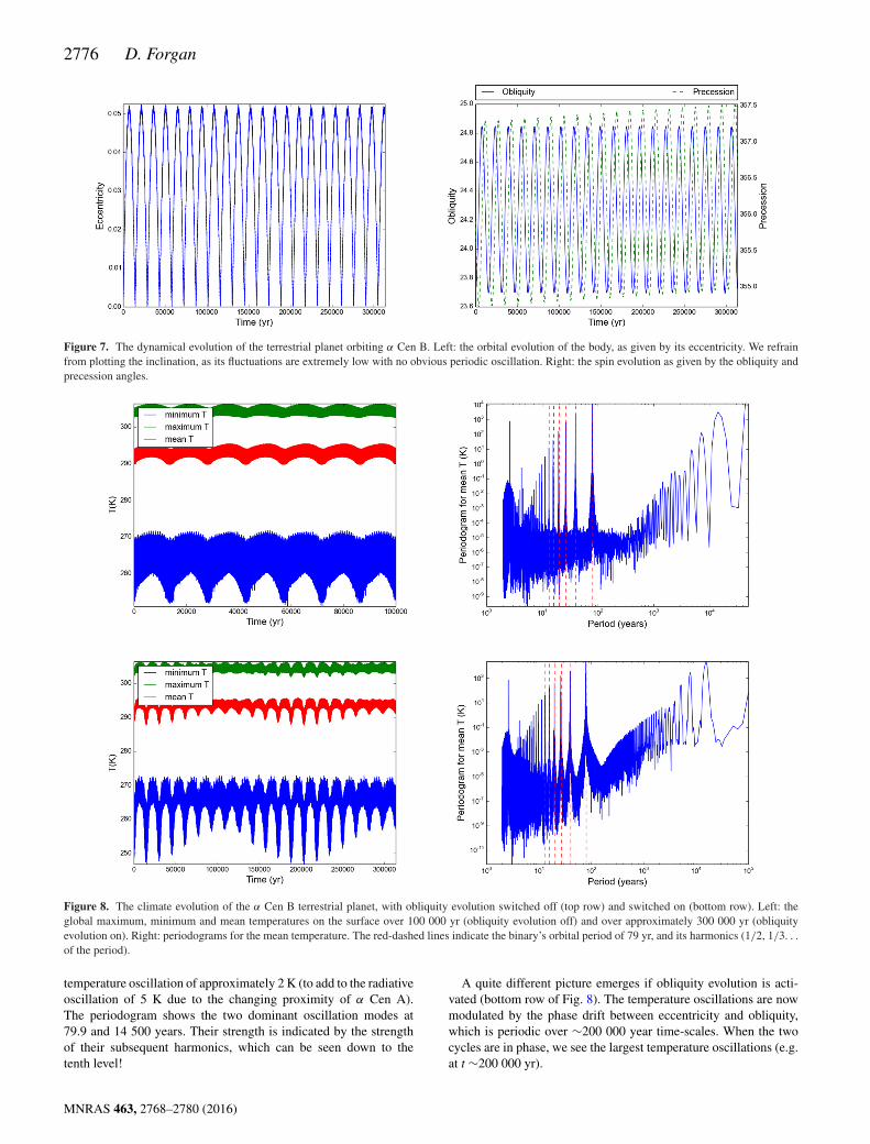
Figure 7. The dynamical evolution of the terrestrial planet orbiting α Cen B. Left: the orbital evolution of the body, as given by its eccentricity. We refrainfrom plotting the inclination, as its fluctuations are extremely low with no obvious periodic oscillation. Right: the spin evolution as given by the obliquity andprecession angles.

Figure 8. The climate evolution of the α Cen B terrestrial planet, with obliquity evolution switched off (top row) and switched on (bottom row). Left: theglobal maximum, minimum and mean temperatures on the surface over 100 000 yr (obliquity evolution off) and over approximately 300 000 yr (obliquityevolution on). Right: periodograms for the mean temperature. The red-dashed lines indicate the binary’s orbital period of 79 yr, and its harmonics (1/2, 1/3. . .of the period).

temperature oscillation of approximately 2 K (to add to the radiativeoscillation of 5 K due to the changing proximity of α Cen A).The periodogram shows the two dominant oscillation modes at79.9 and 14 500 years. Their strength is indicated by the strengthof their subsequent harmonics, which can be seen down to thetenth level!

A quite different picture emerges if obliquity evolution is acti-vated (bottom row of Fig. 8). The temperature oscillations are nowmodulated by the phase drift between eccentricity and obliquity,which is periodic over ∼200 000 year time-scales. When the twocycles are in phase, we see the largest temperature oscillations (e.g.at t ∼200 000 yr).

MNRAS 463, 2768–2780 (2016)

Milankovitch cycles in binary systems 2777

Figure 9. The dynamical evolution of the terrestrial planet orbiting α Cen B. Left: the orbital evolution of the body, as given by its eccentricity and inclination.Right: the spin evolution as given by the obliquity and precession angles.

3.2.3 Adding a planet in 3:2 mean motion resonance

We now consider joint planetary-binary Milankovitch cycles byadding an Earth mass planet on a circular orbit at 0.9293 au, plac-ing it in 3:2 mean motion resonance with the habitable planet. Testruns with α Cen A absent show the additional planet induces regulareccentricity oscillations in the habitable planet with amplitude ofapproximately 0.01, and a period of approximately 500 yr. Inciden-tally, the absence of α Cen A would also place both planets outsidethe HZ.

With α Cen A present, the combination of stellar and planetaryforcings produces eccentricity oscillations of maximum amplitude0.08 (left-hand panel of Fig. 9) and with a mix of dominant periods,as opposed to the distinct 14 500 year period observed in the singleplanet case. The inclination varies with a period of approximately30 000 yr, with a distinctive shift in mean inclination of around 0.001radians (i.e. 0.05◦). The obliquity and precession continue to evolveat close to the eccentricity oscillation period, but the amplitude oftheir oscillations varies on approximately twice this time-scale.

The uniform temperature evolution cycles seen in Fig. 8 are nowmore confused with the addition of a neighbour planet (Fig. 10).With obliquity evolution switched off (top row), the extra structureintroduced into the eccentricity and inclination oscillations leavesan imprint on the temperature curves. This can be seen in its pe-riodogram (top-right panel of Fig. 10), which shows a relativelyweak feature at the perturbing planet’s orbital period, and at the res-onant period of twice the perturber’s period (or equivalently, threetimes the habitable planet’s period). The perturbations induced bythe additional planet produce temperature variations of up to 2 Kcompared to the single planet case.

With obliquity evolution turned on (bottom panel), the eccen-tricity/obliquity relationship seen in the previous case is preserved,resulting in phase drift between the two oscillations. However, theextra structure in the eccentricity oscillation prevents the smoothamplitude modulation of temperature that we saw in the bottomright panel of Fig. 8. It is broadly present, but heavily modifiedby the presence of the neighbouring planet. The periodogram stillreveals weak signals at the perturbing planet’s period, and thestrong peak feature at approximately 14 500 yr is now split intwo. There is also a significant increase in signal for periods oforder 100–1000 yr.

Additional giant planets in a system like this might be expectedto produce even larger excursions from circular orbits and stronger

Milankovitch cycling. Given that planet formation models disfavourthe creation of Jupiter mass bodies in this system (Xie et al. 2010)and are ruled out by observations of the α Cen system, at least atperiods less than ∼1 yr (Endl et al. 2001; Dumusque et al. 2012;Demory et al. 2015) this is not a particular concern. But, one mightimagine that undetected Neptune mass bodies could be present inthis system on relatively long period orbits, and such bodies wouldbe responsible for longer period Milankovitch cycles similar to thatof Earth’s.

4 D I SCUSSI ON

4.1 Limitations of the model

LEBM modelling is by its definition a compromise between thegranularity of a climate simulation and computational expediency.This compromise is stretched further by the coupling of the N-BODY integrator and obliquity evolution. We have adopted a verysimple coupling where both the N-Body and LEBM componentsare constrained to follow the same global timestep.

This timestep system works extremely well for systems where thedynamical time-scale is relatively long, such as the S-type binarysystems. In this scenario, the system timestep is limited only by theLEBM, and as such we can run simulations with similar wallclocktimes as that of a LEBM using fixed Keplerian orbits. However, inthe P-type scenario, the dynamical time-scale is relatively short, andthe system is limited by the N-Body timestep required to resolvethe binary.

There are several possible strategies for mitigating this timestepissue. The most straightforward solution is to adopt a non-sharedtimestep for the N-Body component, allowing some of the bodiesto possess shorter N-Body timesteps. This would reduce the com-putational load of evolving all the bodies (and the LEBM) at whatcan be very short timesteps. Another solution would require the in-terpolation of body motions (in the case where the LEBM timestepis small compared to the N-Body timestep), but this would likelyproduce only marginal gains in speed. Perhaps the best solution forP-type systems would be chain regularisation of the tight binaryorbit (Mikkola & Aarseth 1990, 1993).

Aside from the new challenges arising from the adoption of theN-Body integrator, there are the usual limitations that many LEBMsare subject to. Our implementation of the LEBM is among the most

MNRAS 463, 2768–2780 (2016)

2778 D. Forgan

Figure 10. The climate evolution of the α Cen B terrestrial planet, with obliquity evolution switched off (top row) and switched on (bottom row). Left: theglobal maximum, minimum and mean temperatures on the surface over 100 000 yr (obliquity evolution off) and over approximately 300 000 yr (obliquityevolution on). Right: periodograms for the mean temperature. The red-dashed lines indicate the binary’s orbital period of 79 yr, and its harmonics (1/2, 1/3. . .of the period).

simple available which can still broadly reproduce the seasonaltemperature profiles of a fiducial Earth model. The principal ad-vantage of this simplicity is its ease of interpretation, but we mustacknowledge that more advanced models may produce features wecannot.

For example, we do not model the carbonate-silicate (CS) cy-cle, which moderates fluctuations in atmospheric temperature byincreasing and reducing the partial pressure of carbon dioxide. Thetime-scale on which we expect CO2 levels to vary depends onthe planet’s geochemical properties, especially its ocean circula-tion. For Earth-like planets, the equilibriation time-scale of CO2

is approximately half a million years (Williams & Kasting 1997)which is far shorter than the Milankovitch cycles experienced bythe planetary bodies in this analysis. However, our understand-ing of the CS cycle is rooted firmly in our understanding of theEarth, which orbits a single star. It remains unclear whether aplanet in a binary star system would possess a similar equilib-riation time-scale, even if the planet was effectively identical tothe Earth.

While we have taken the first steps towards coupling celestialdynamics and LEBM climate modelling here, there are still severalsteps ahead of us. For example, the tidal interactions between bodieswill also modify orbits of habitable worlds, in particular reducingtheir eccentricity and modifying their rotational period (Bolmontet al. 2014; Cunha, Correia & Laskar 2014). While this is unlikelyto be an issue for the orbital configurations adopted in this analysis,

it remains the case that while the tidal interactions between thebinary stars is well characterized (e.g. Mason et al. 2013; Zuluagaet al. 2016), the tidal evolution of planets in P-type systems remainsrelatively unexplored.

Also to be explored in full are the obliquity variations felt byplanets in binary systems. We have adopted a set of equationsdesigned for a single star planetary system, and assumed theyare valid when there are two stars present. In effect we have as-sumed that in S-type systems, the secondary’s direct tidal torque onplanetary spin is negligible, and that in P-type systems the directtorques always co-add. Is this always the case? More investigationis needed.

We should also note that the strength of Milankovitch cyclesmeasured by the LEBM will be an underestimate. Tests conductedusing Solar system parameters (Forgan & Mead, in preparation)give Milankovitch cycles for the Earth that are an order of mag-nitude smaller in temperature variation than observed in paleocli-mate data (Zachos et al. 2001; Lisiecki & Raymo 2005). Para-doxically, stochastic EBMs, with additional random noise, can en-hance periodic variations through the phenomenon of stochasticresonance (Imkeller 2001; Benzi 2010). Obliquity variation doesproduce a much richer set of temperature variations on decadaltime-scales, which may be forced into stochastic resonant behaviourunder appropriate circumstances. Future investigations should con-sider adding a random noise term to the LEBM equation to permitthis behaviour.

MNRAS 463, 2768–2780 (2016)

Milankovitch cycles in binary systems 2779

4.2 Implications for habitability

So what have we gained by this coupling of N-Body and LEBMintegrators? Initially, we are able to confirm that in general, thedecoupled approach of considering the radiative and gravitationalperturbations separately is broadly acceptable.

Previous work in this field is not invalidated by our results, butit makes explicit some general principles that are already knownimplicitly. First, the HZ of a planetary system is defined by morethan where the radiation sources are in the system. The gravita-tional sources are equally important. We know this on Earth thanksto our understanding of Milankovitch cycles, and the Earth’s orbitaland spin cycles are relatively weak when compared to measuredcycles for Earth-like planets in typical exoplanet system configura-tions around a single star (Spiegel et al. 2010, Forgan & Mead, inpreparation).

Secondly, the HZ of binary systems is even more sensitive to thegravitational field than single star systems. This is already demon-strated implicitly by the N-Body simulations of orbital stabilitydiscussed in the Introduction. Our results clearly identify the effectof orbital and spin stability on climate. We show that relativelystrong Milankovitch cycles exist in binary systems, even if there isonly one planet present. The periods of these cycles are in generalshorter than that of single star systems, but of similar amplitudes.Even on short time-scales, the radiative perturbations induced overthe orbital period of the binary are detectable in the mean tempera-ture of the planet.

Thirdly, the circadian rhythms of life on planets in binary systemswill be forced to adapt to the rhythms present in the binary system,as is evidenced by analogous studies of lunar photoperiodism in ter-restrial organisms (O’Malley-James et al. 2012; Forgan et al. 2015and references within). Temperature fluctuations of several K ontime-scales ranging from less than a year to almost a century (de-pending on whether the system is P- or S-type) is likely to producesignificant fluctuations in surface coverage of biomes. The rapidMilankovitch cycles are likely to play a stronger role also. Moresophisticated climate models coupled to N-Body physics (for ex-ample, 3D global circulation models) may show potential for more,shorter Ice Ages, and briefer interglacial periods. The presence ofsuch rapid changes to environmental selection pressure will have anindelible effect on the evolution of organisms in binary planetarysystems. Future work should build on recent attempts to produce3D General Circulation Models of circumbinary planets (cf. May &Rauscher 2016), incorporating the systems’ gravitational evolutionto determine these effects in detail.

5 C O N C L U S I O N S

We have investigated Milankovitch cycles both circumbinary (P-type) and distant binary (S-type) systems, using Kepler-47 and α

Centauri as archetypes. To do this, we coupled a 1D latitudinalenergy balance climate model (LEBM) with an N-Body integratorto follow the orbital evolution, and an obliquity evolution algorithmto study the spin-axis evolution.

We find that the combined spin–orbit-radiative perturbations in-duced by a companion star on a habitable planet produce Mi-lankovitch cycles for both types of binary system, even when otherplanets are not present. Periodogram analysis identifies both dy-namical and secular oscillations in the mean temperature of planetsin these systems, over a variety of short and long periods, as wellas the presence of radiative perturbations directly linked to the pe-riod of the binary. The strength of these oscillations is sensitive to

the orbital configuration of the system. The relative phase betweeneccentricity, precession and obliquity cycles is important, just as itis for the Earth.

In general, we find these Milankovitch cycles are significantlyshorter than comparable cycles on the Earth (in some cases shorterthan 1000 yr), although the amplitude of the changes they produce inthe planets’ orbital elements are comparable to those experienced byEarth. This work demonstrates the need to consider joint dynamics–climate simulations of habitable worlds in binary systems, if we areto truly assess the potential for the birth and growth of biosphereson worlds with two suns.

AC K N OW L E D G E M E N T S

DHF gratefully acknowledges support from the ECOGAL project,grant agreement 291227, funded by the European Research Councilunder ERC-2011-ADG. This work relied on the compute resourcesof the St Andrews MHD Cluster. The author thanks both NaderHaghighipour and James Gilmore for insightful comments on anearly version of this manuscript. This research has made use ofNASA’s Astrophysics Data System Bibliographic Services. Thecode used in this work is now available open source as OBERON,which can be downloaded at github.com/dh4gan/oberon.

R E F E R E N C E S

Anderson K. R., Storch N. I., Lai D., 2016, MNRAS, 456, 3671Andrade-Ines E., Michtchenko T. A., 2014, MNRAS, 444, 2167Armstrong J. C., Leovy C. B., Quinn T., 2004, Icarus, 171, 255Armstrong D. J., Osborn H. P., Brown D. J. A., Faedi F., Gomez Maqueo

Chew Y., Martin D. V., Pollacco D., Udry S., 2014a, MNRAS, 444, 1873Armstrong J. C., Barnes R., Domagal-Goldman S., Breiner J., Quinn T. R.,

Meadows V. S., 2014b, Astrobiology, 14, 277Benzi R., 2010, Nonlinear Process. Geophys., 17, 431Bolmont E., Raymond S. N., von Paris P., Selsis F., Hersant F., Quintana

E. V., Barclay T., 2014, ApJ, 793, 3Brown S., Mead A., Forgan D., Raven J., Cockell C., 2014, Int. J. Astrobiol.,

13, 279Chavez C. E., Georgakarakos N., Prodan S., Reyes-Ruiz M., Aceves H.,

Betancourt F., Perez-Tijerina E., 2014, MNRAS, 446, 1283Cuartas-Restrepo P., Melita M., Zuluaga J., Portilla B., Sucerquia M., Miloni

O., 2016, MNRAS, preprint (arXiv:1606.07546)Cunha D., Correia A. C., Laskar J., 2014, Int. J. Astrobiol., 14, 233Cuntz M., 2014, ApJ, 780, 14Del Genio A., 1993, Icarus, 101, 1Del Genio A., 1996, Icarus, 120, 332Demory B.-O. et al., 2015, MNRAS, 450, 2043Desidera S., Barbieri M., 2007, A&A, 462, 345Doolin S., Blundell K. M., 2011, MNRAS, 418, 2656Doyle L. R. et al., 2011, Science, 333, 1602Dressing C. D., Spiegel D. S., Scharf C. A., Menou K., Raymond S. N.,

2010, ApJ, 721, 1295Dumusque X. et al., 2012, Nature, 491, 207Dunhill A. C., Alexander R. D., 2013, MNRAS, 435, 2328Duquennoy A., Mayor M., 1991, A&A, 248, 485Dvorak R., 1984, Celest. Mech., 34, 369Dvorak R., 1986, A&A, 167, 379Eggl S., Pilat-Lohinger E., Georgakarakos N., Gyergyovits M., Funk B.,

2012, ApJ, 752, 74Endl M., Krster M., Els S., Hatzes A. P., Cochran W. D., 2001, A&A, 374,

675Farrell B. F., 1990, J. Atmos. Sci., 47, 2986Forgan D., 2012, MNRAS, 422, 1241Forgan D., 2014, MNRAS, 437, 1352

MNRAS 463, 2768–2780 (2016)

2780 D. Forgan

Forgan D. H., Mead A., Cockell C. S., Raven J. A., 2015, Int. J. Astrobiol.,14, 465

Haghighipour N., Kaltenegger L., 2013, ApJ, 777, 166Hart M., 1979, Icarus, 37, 351Hatzes A. P., 2013, ApJ, 770, 133Hatzes A. P., Cochran W. D., Endl M., McArthur B., Paulson D. B., Walker

G. A. H., Campbell B., Yang S., 2003, ApJ, 599, 1383Holman M. J., Wiegert P. A., 1999, AJ, 117, 621Huang S.-S., 1959, PASP, 71, 421Imkeller P., 2001, in Imkeller P., Von Storch J.-S., eds, Stochastic Climate

Models. Birkhauser, Basel, p. 213Jaime L. G., Aguilar L., Pichardo B., 2014, MNRAS, 443, 260Kaltenegger L., Haghighipour N., 2013, ApJ, 777, 165Kane S. R., Hinkel N. R., 2013, ApJ, 762, 7Kasting J., Whitmire D., Reynolds R., 1993, Icarus, 101, 108Kopparapu R. K. et al., 2013, ApJ, 765, 131Kopparapu R. K., Ramirez R. M., SchottelKotte J., Kasting J. F., Domagal-

Goldman S., Eymet V., 2014, ApJ, 787, L29Kostov V. B. et al., 2014, ApJ, 784, 14Laskar J., 1986a, A&A, 164, 437Laskar J., 1986b, A&A, 157, 59Lisiecki L. E., Raymo M. E., 2005, Paleoceanography, 20, PA1003Martin R. G., Armitage P. J., Alexander R. D., 2013, ApJ, 773, 74Marzari F., Thebault P., Scholl H., Picogna G., Baruteau C., 2013, A&A,

553, A71Mason P. A., Zuluaga J. I., Clark J. M., Cuartas-Restrepo P. A., 2013, ApJ,

774, L26May E. M., Rauscher E., 2016, ApJ, 826, 225Meschiari S., 2014, ApJ, 790, 41Mikkola S., Aarseth S. J., 1990, Celest. Mech. Dyn. Astron., 47, 375Mikkola S., Aarseth S. J., 1993, Celest. Mech. Dyn. Astron., 57, 439O’Malley-James J. T., Raven J. A., Cockell C. S., Greaves J. S., 2012,

Astrobiology, 12, 115Orosz J. A. et al., 2012, Science, 337, 1511Pichardo B., Sparke L. S., Aguilar L. A., 2005, MNRAS, 359, 521Pierrehumbert R. T., 2005, J. Geophys. Res., 110, D01111Pilat-Lohinger E., Dvorak R., 2002, Celest. Mech. Dyn. Astron., 82, 143Queloz D. et al., 2000, A&A, 354, 99Quintana E. V., Lissauer J. J., Chambers J. E., Duncan M. J., 2002, ApJ,

576, 982

Quintana E. V., Adams F. C., Lissauer J. J., Chambers J. E., 2007, ApJ, 660,807

Rafikov R. R., 2013, ApJ, 764, L16Rafikov R. R., Silsbee K., 2014a, ApJ, 798, 69Rafikov R. R., Silsbee K., 2014b, ApJ, 798, 70Raghavan D. et al., 2010, ApJS, 190, 1Rajpaul V., Aigrain S., Roberts S., 2016, MNRAS, 456, L6Sigurdsson S., Richer H. B., Hansen B. M., Stairs I. H., Thorsett S. E., 2003,

Science, 301, 193Silsbee K., Rafikov R. R., 2015, ApJ, 798, 71Spiegel D. S., Menou K., Scharf C. A., 2008, ApJ, 681, 1609Spiegel D. S., Raymond S. N., Dressing C. D., Scharf C. A., Mitchell J. L.,

2010, ApJ, 721, 1308Tajika E., 2008, ApJ, 680, L53Thebault P., Marzari F., Scholl H., 2008, MNRAS, 388, 1528Thebault P., Marzari F., Scholl H., 2009, MNRAS, 393, L21Thevenin F., Provost J., Morel P., Berthomieu G., Bouchy F., Carrier F.,

2002, A&A, 392, L9Thorsett S. E., Arzoumanian Z., Taylor J. H., 1993, ApJ, 412, L33Vladilo G., Murante G., Silva L., Provenzale A., Ferri G., Ragazzini G.,

2013, ApJ, 767, 65Welsh W. F. et al., 2012, Nature, 481, 475Welsh W. F. et al., 2015, ApJ, 809, 26Wertheimer J. G., Laughlin G., 2006, AJ, 132, 1995Wiegert P. A., Holman M. J., 1997, AJ, 113, 1445Williams D., Kasting J., 1997, Icarus, 129, 254Xie J.-W., Zhou J.-L., Ge J., 2010, ApJ, 708, 1566Zachos J., Pagani M., Sloan L., Thomas E., Billups K., 2001, Science, 292,

686Zucker S., Mazeh T., Santos N. C., Udry S., Mayor M., 2004, A&A, 426,

695Zuluaga J. I., Mason P. A., Cuartas-Restrepo P. A., 2016, ApJ, 818, 160

This paper has been typeset from a TEX/LATEX file prepared by the author.

MNRAS 463, 2768–2780 (2016)