CS 261Fall 2018

Mike Lam, Professor

Memory

Topics

● Memory hierarchy overview● Storage technologies● I/O architecture● Storage trends● Latency comparisons● Locality

Memory

● Until now, we've referred to “memory” as a black box● Modern systems actually have a variety of memory types

called a memory hierarchy– Frequently-accessed data in faster memory– Each level caches data from the next lower level

● Goal: large general pool of memory that performs almost as well as if it was all made of the fastest memory

● Key concept: locality of time and space● Other useful distinctions:

– Volatile vs. non-volatile– Random access vs sequential access

Memory hierarchy

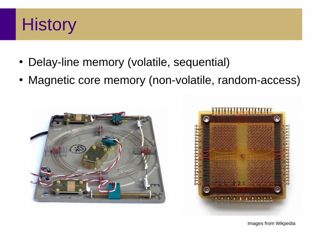
History

● Delay-line memory (volatile, sequential)● Magnetic core memory (non-volatile, random-access)

Images from Wikpedia

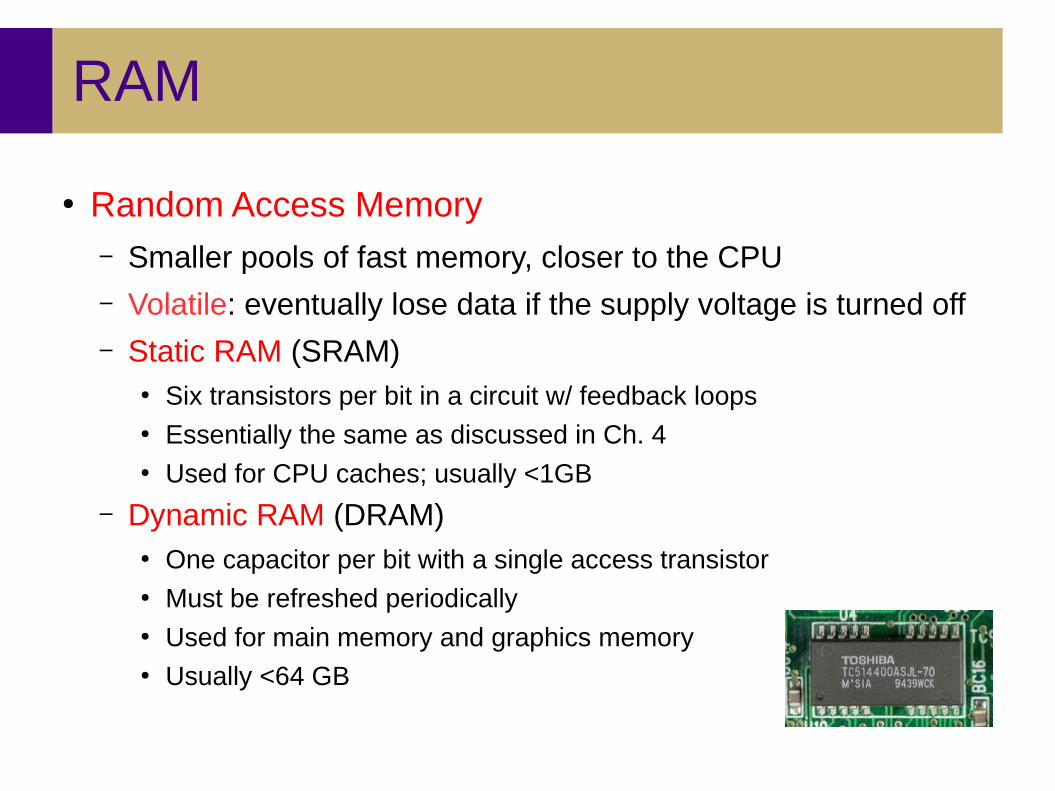
RAM

● Random Access Memory– Smaller pools of fast memory, closer to the CPU– Volatile: eventually lose data if the supply voltage is turned off– Static RAM (SRAM)

● Six transistors per bit in a circuit w/ feedback loops● Essentially the same as discussed in Ch. 4● Used for CPU caches; usually <1GB

– Dynamic RAM (DRAM)● One capacitor per bit with a single access transistor● Must be refreshed periodically● Used for main memory and graphics memory● Usually <64 GB

DRAM

● DRAM chips store data in a grid of supercells● Memory controller used to access data

– Connected to CPU via memory bus– Row access strobe (RAS) request– Column access strobe (CAS) request

Enhanced DRAM

● Fast page mode DRAM (FPM DRAM)– Serve same-row accesses from a row buffer

● Extended data out DRAM (EDO DRAM)– Allow CAS signals to be more closely spaced

● Synchronous DRAM (SDRAM)– Use a clock to synchronize and speed accesses

● Double data-rate SDRAM (DDR SDRAM)– Use both rising and falling edges of clock signal

● Video RAM (VRAM)– Shift an entire buffer's contents in a single operation– Allow simultaneous reads and writes

Nonvolatile memory

● Nonvolatile memory retains data if the supply voltage is turned off– Historically referred to as read-only memory (ROM)– Newer forms of nonvolatile memory can be written

● Programmable ROM (PROM)– Programmed only once by blowing fuses

● Erasable PROM (EPROM)– Re-programmed using ultraviolet light

● Electrically-erasable PROM (EEPROM)– Re-programmed using electric signals– Basis for flash memory storage devices

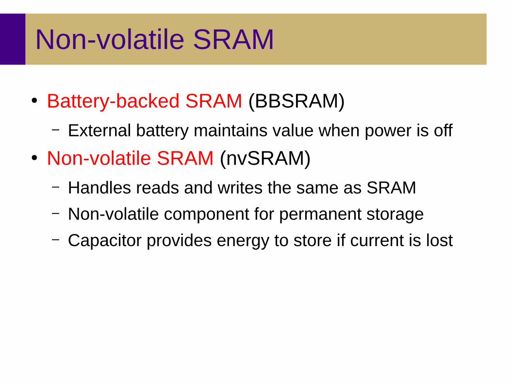
Non-volatile SRAM

● Battery-backed SRAM (BBSRAM)– External battery maintains value when power is off

● Non-volatile SRAM (nvSRAM)– Handles reads and writes the same as SRAM– Non-volatile component for permanent storage– Capacitor provides energy to store if current is lost

Disk storage

● Disk storage systems hold large amounts of data– More cost effective than SRAM or DRAM– Usually order of magnitudes slower

● Solid-state drives (SSDs)– Flash memory organized into blocks

● Traditional magnetic hard disk drives (HDDs)– Multiple platters with surfaces coated with magnetic material– Accessed using a physical arm with a magnetic head– Data stored on surface in tracks partitioned into sectors

Hard disk drives

● Capacity is based on areal density– Product of recording density and track density

● Operation requires mechanical motion– Magnetic read/write head on an actuator arm

● Speed is based on average access time– Sum of seek time, rotational latency, and transfer time– Platters spin at standard rate

● Disk controller coordinates accesses– Maps logical blocks to (surface, track, sector) numbers

Tape and network storage

● Archival storage systems provide large-scale data storage– Lowest cost per byte, but slowest access

● Tape drives store data on magnetic tape– Often in an off-site location for added redundancy

● Network-attached storage (NAS) systems– Dedicated data storage server– Often uses redundant disks for reliability (RAID)– Communicate over a network via a file sharing protocol– Examples: NFS, Samba, AFS– More about this in CS 361 and CS 470!

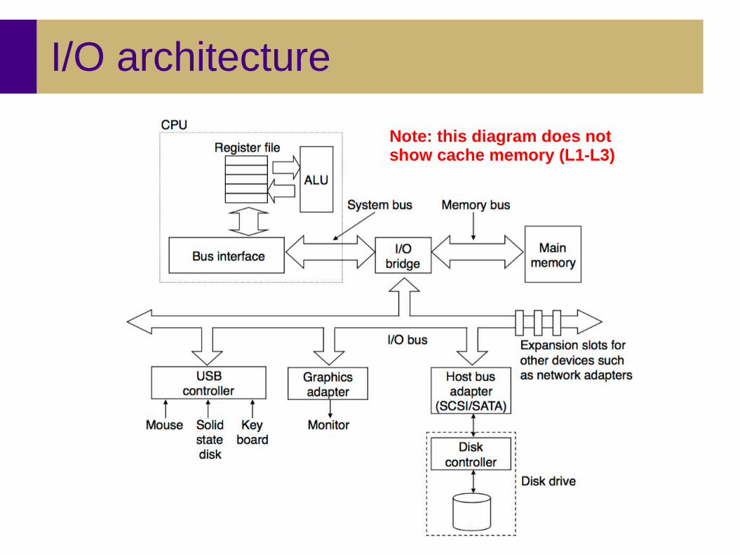
I/O architecture

Note: this diagram does not show cache memory (L1-L3)

I/O architecture

● Cache memory (SRAM)– Access via direct connection to CPU (or on-die)

● Main memory (DRAM)– Bus transactions via I/O bridge on motherboard

● Disk drives (magnetic disk & SSD)– Connected to I/O bridge via I/O bus– Requires a device controller for communication– Memory transactions w/o CPU via direct memory access (DMA)– Technologies: USB, SATA, SCSI

● Other memory (graphics, network storage)– Connected to I/O bus using expansion slots on motherboard

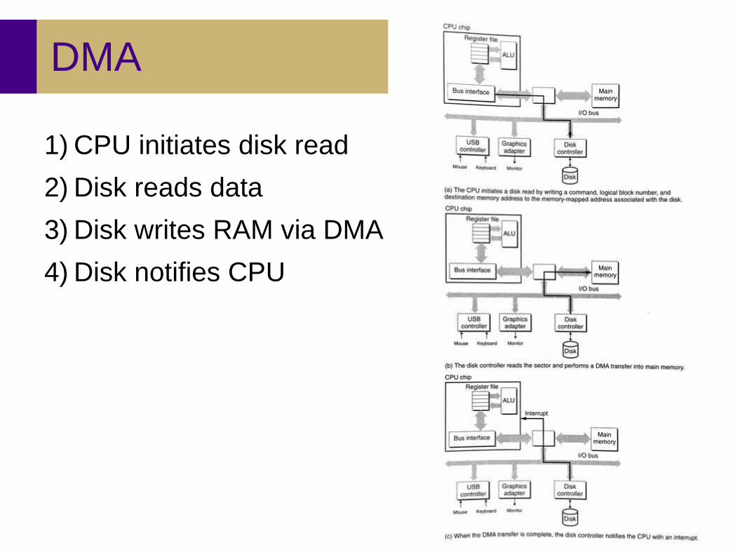
DMA

1) CPU initiates disk read

2) Disk reads data

3) Disk writes RAM via DMA

4) Disk notifies CPU

Technology comparison

(w/ multicore CPUs)

Storage trends

Fasterandcheaper

Effective cycle times continue to decrease

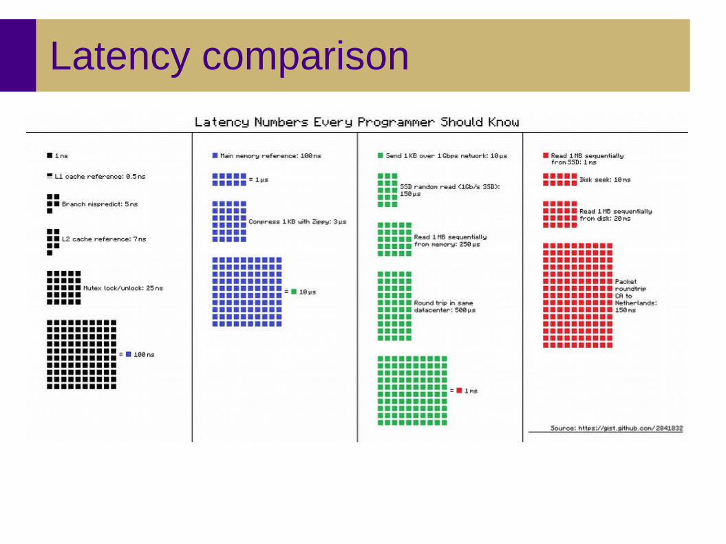
Latency comparison

Latency comparisonLets multiply all these durations by a billion: (originally from https://dzone.com/articles/every-programmer-should-know)

Minute: L1 cache reference (0.5s) - One heart beat L2 cache reference (7s) - Long yawn

Hour: Main memory reference (100s) - Brushing your teeth

Day: Send 2K bytes over 1 Gbps network (5.5 hr) - From lunch to end of work day

Week: SSD random read (1.7 days) - A normal weekend Read 1 MB sequentially from memory (2.9 days) - A long weekend Read 1 MB sequentially from SSD (11.6 days) - Waiting for almost 2 weeks for a delivery

Year: Disk seek (16.5 weeks) - A semester in university Read 1 MB sequentially from disk (7.8 months) – Two semesters in university The above 2 together (1 year)

Decade: Send packet CA->Netherlands->CA (4.8 years) - Completing a bachelor's degree

Locality

● Temporal locality: frequently-accessed items will continue to be accessed in the future– Theme: repetition is common

● Spatial locality: nearby addresses are more likely to be accessed soon– Theme: sequential access is common

● Why do we care?– Programs with good locality run faster than programs with

poor locality

Data locality

● Temporal locality: keep often-used values in higher tiers of the memory hierarchy

● Spatial locality: use predictable access patterns– Stride-1 reference pattern (sequential access)– Stride-k reference pattern (every k elements)– Closely related to row-major vs. column-major– Allows for prefetching (predicting the next needed

element and preloading it)

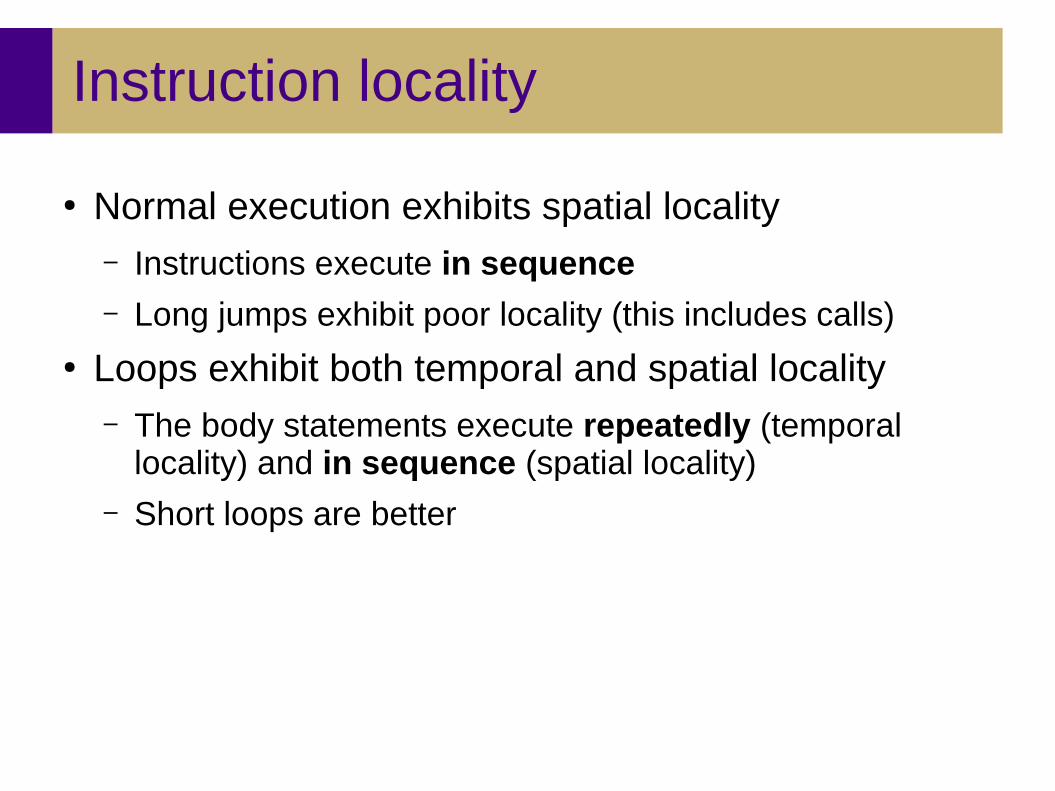
Instruction locality

● Normal execution exhibits spatial locality– Instructions execute in sequence– Long jumps exhibit poor locality (this includes calls)

● Loops exhibit both temporal and spatial locality– The body statements execute repeatedly (temporal

locality) and in sequence (spatial locality)– Short loops are better

Example

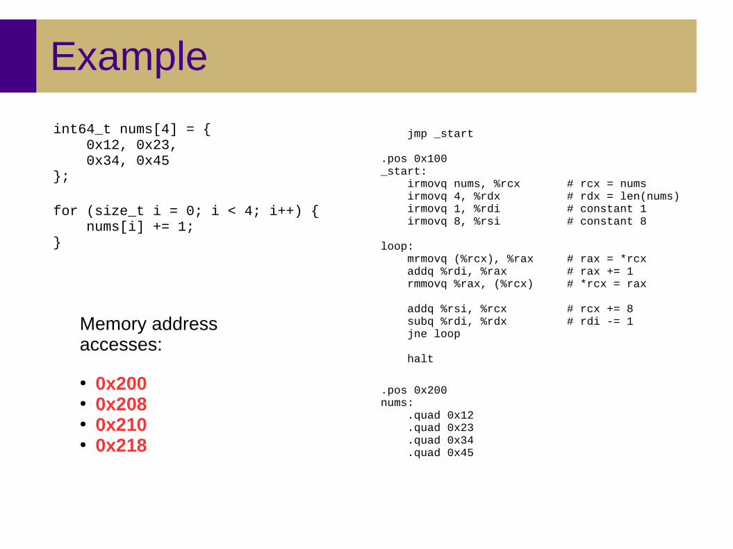
jmp _start .pos 0x100_start: irmovq nums, %rcx # rcx = nums irmovq 4, %rdx # rdx = len(nums) irmovq 1, %rdi # constant 1 irmovq 8, %rsi # constant 8 loop: mrmovq (%rcx), %rax # rax = *rcx addq %rdi, %rax # rax += 1 rmmovq %rax, (%rcx) # *rcx = rax addq %rsi, %rcx # rcx += 8 subq %rdi, %rdx # rdi -= 1 jne loop halt

.pos 0x200nums: .quad 0x12 .quad 0x23 .quad 0x34 .quad 0x45

int64_t nums[4] = { 0x12, 0x23, 0x34, 0x45 };

for (size_t i = 0; i < 4; i++) { nums[i] += 1; }

Memory address accesses:

● 0x200● 0x208● 0x210● 0x218

Core themes

● Systems design involves tradeoffs– Memory: price vs. performance (e.g., DRAM vs. SRAM)

● The details matter!– Knowledge of the underlying system enables you to

exploit latency inequalities for better performance● Key concepts: locality and caching

– Store and access related things together– Keep copies of things you’ll need again soon– We’ll look at these more next time