MIGRATION TIMING AND STOPOVER SELECTION FOR … · 2017. 3. 7. · barnacle goose populations,...
147
MIGRATION TIMING AND STOPOVER SELECTION FOR BARNACLE GEESE BRANTA LEUCOPSIS Mitra Shariati Najafabadi
Transcript of MIGRATION TIMING AND STOPOVER SELECTION FOR … · 2017. 3. 7. · barnacle goose populations,...

MIGRATION TIMING AND STOPOVER SELECTION FOR BARNACLE GEESE BRANTA LEUCOPSIS
Mitra Shariati Najafabadi

Graduation committee: Chairman/Secretary Prof.dr.ir. A. Veldkamp Supervisor Prof.dr. A.K. Skidmore University of Twente Prof.dr. P.J.M. Havinga University of Twente Co-supervisor Dr. R. Darviszadeh Varchehi University of Twente Members Prof.dr.ir. A. Veldkamp University of Twente Prof.dr.ir. M.F.A.M. van Maarseveen University of Twente Prof.dr. J. Madsen Aarhus University Prof.dr. R. Real Giménez University of Malaga Dr.ir. R.A. de By University of Twente ITC dissertation number 300 ITC, P.O. Box 217, 7500 AA Enschede, The Netherlands ISBN 978-90-365-4318-7 DOI 10.3990/1.9789036543187 Cover designed by Mitra Shariati Najafabadi Printed by ITC Printing Department Copyright © 2017 by Mitra Shariati Najafabadi

MIGRATION TIMING AND STOPOVER SELECTION FOR BARNACLE GEESE BRANTA LEUCOPSIS
DISSERTATION
to obtain the degree of doctor at the University of Twente,
on the authority of the rector magnificus, prof.dr. T.T.M. Palstra,
on account of the decision of the graduation committee, to be publicly defended
on Thursday 23 March 2017 at 14:45 hrs
by
Mitra Shariati Najafabadi
born on September 19th 1983 in Najafabad, Iran

This thesis is approved by Prof. dr. A. K. Skidmore, supervisor Prof. dr. P.J.M. Havinga, supervisor Dr. R. Darvishzadeh Varchehi, co-supervisor

Acknowledgements Pursuing a Ph.D. project is a both painful and enjoyable experience. It can be compared to climbing a high peak, step by step, fraught with bitterness, hardships, frustration, but met with encouragement, trust and help of several people. After five years of hard work, I found myself at the top of the accomplished summit enjoying the beautiful scenery. I realized that teamwork got me there, and sans the help from my supporters, I would have failed to complete this work. I am earnestly grateful to each and every one of these people, especially the ones who constantly supported me within the past five years: Firstly, I would like to express my sincere gratitude to my promoters, Prof. Andrew Skidmore and Prof. Paul Havinga for their continuous support of my Ph.D. study and related research. In particular, I would like to thank Prof. Skidmore for his patience, motivation, and immense knowledge. His guidance helped and inspired me throughout the research and thesis writing. Besides my promoters, I would like to thank my co-promoter Dr. Roshanak Darvishzadeh, for her insightful comments and encouragement, but also for the questions which encouraged me to widen my research from various perspectives. I also thank Dr. Albertus Toxopeus for his multifaceted involvement in my research and for his input on my papers. Extending my sincere thanks to Prof. Bart Nolet, Dr. Klaus-Michael Exo, Dr. Larry Griffin, Dr. Andrea Kölzsch, Dr. Julia Stahl, and Dr. David Cabot. I am grateful to them for providing the geese data and sharing interesting and fruitful comments on my papers. I would like to thank staff members of the NRS, in particular, Dr. Tiejun Wang and Dr. Anton Vrieling as well as, Dr. Nirvana Meratnia from the Faculty of Electrical Engineering for their assistance. My special thanks to Mr. Willem Nieuwenhuis for helping me with the programming and his technical assistance. I also would like to thank Ms. Esther Hondebrink, Ms. Loes Colenbrander, Ms. Angelique Holtkamp, Ms. Theresa van den Boogaard, Dr. Tom Rientjes, Mr. Benno Masselink, and Mr. Roelof Schoppers for their excellent service. I am also indebted to the European Commission’s Erasmus Mundus program for awarding me Ph.D. scholarship and Faculty of Geo-information Science and Earth Observation (ITC) for the financial support. Without their support, it would not have been possible for me to undertake this research.

ii
My cordial thanks go to my office mates Dr. Saleem Ullah, Dr. Mohammad Shafique, Ms. Linlin Li, Dr. Abebe Ali and also to my dear friends in ITC and Enschede. Few of them are: Ms. Parinaz Rashidi, Ms. Efthymia Pavlidou, Dr. Thea Turkington, Mr. Hassan Firouzbakht, Dr. Babak Naimi, Dr. Sanaz Salati, Dr. Abel Ramoelo, Mr. Sam Khosravifard, Ms. Elnaz Neinavaz, Ms. Anahita Khosravipour, Dr. Anandita Sengupta, Dr. Maitreyi Sur, Dr. Abas Farshad, Ms. Sonia Farshad, Mr. Davood Baratian, Ms. Hengame Noushahri, Ms. Fangyuan Yu, Ms. Adish Khezri, Ms. Sara Mehryar, Ms. Azar Zafari, Ms. Malihe Gholamhosseini and Ms. Shadi Fekri. Last but not the least, I would like to thank my family, my parents and my sister for supporting me spiritually throughout my life and particularly during the writing of this thesis.

iii
Table of Contents Acknowledgements ............................................................................... i Preface ............................................................................................... ii Table of Contents ................................................................................ iii List of Figures ..................................................................................... vi List of tables....................................................................................... ix Chapter 1: General Introduction .............................................................1
1.1 Background ................................................................... 2 1.2 Barnacle geese and research problem ................................... 4
1.2.1 New index to test green wave hypothesis for barnacle geese ..4 1.2.2 Knowledge gaps about the relevance of environmental conditions at last staging site for migration timing ....................5 1.2.3 Stopover selection ...............................................................5
1.3 Research Objective .......................................................... 6 1.4 Study area .................................................................... 6 1.5 Thesis Outline ................................................................ 7
Chapter 2: Migratory herbivorous waterfowl track satellite-derived green wave index ..........................................................................................9
2.1 Introduction ................................................................. 11 2.2 Materials and Methods ..................................................... 13
2.2.1 Study area and barnacle goose populations ........................... 13 2.2.2 MODIS NDVI data .............................................................. 14 2.2.3 Satellite-derived green wave index (GWI) ............................. 15 2.2.4 GPS tracking data of barnacle geese..................................... 16 2.2.5 Delineation of stopover sites ............................................... 17 2.2.6 Relating satellite-derived green wave index to barnacle goose migration ......................................................................... 17
2.3 Results ........................................................................ 19 2.3.1 Visualization of barnacle goose migration against satellite- derived GWI ..................................................................... 19 2.3.2 Correlation between barnacle goose spring migration and date of 50% GWI ..................................................................... 21 2.3.3 Comparison of GWI at spring stopover sites for the three flyway populations ............................................................. 22
2.4 Discussion .................................................................... 23 2.4.1 Migratory barnacle geese track satellite-derived green wave index ............................................................................... 23 2.4.2 Differences in the satellite-derived GWI at spring stopover sites ................................................................................ 26
2.5 Conclusions .................................................................. 27 ........... Chapter 3: Satellite- versus temperature-derived green wave indices for predicting the timing of spring migration of avian herbivores .................... 29

iv
3.1 Introduction ................................................................. 31 3.2 Materials and Methods ..................................................... 34 3.2.1 Satellite-derived green wave index (GWI) ............................. 34
3.2.2 Temperature acceleration (GDDjerk) .................................... 34 3.2.3 GPS tracking data .............................................................. 35 3.2.4 Delineation of stopover, and breeding sites ........................... 35 3.2.5 Statistical analysis ............................................................. 36
3.3 Results ........................................................................ 37 3.3.4 Arrival date at the stopover sites ......................................... 37 3.3.5 Arrival date at the breeding site ........................................... 41
3.4 Discussion .................................................................... 43 3.5 Conclusion ................................................................... 45
Chapter 4: Environmental parameters linked to the last migratory stage of barnacle geese en route to their breeding sites ....................................... 47
3.3 Introduction ................................................................. 49 3.4 Materials and Methods ..................................................... 52
3.4.1 Study populations .............................................................. 52 3.4.2 Tracking barnacle geese ..................................................... 53 3.4.3 Ethical note ...................................................................... 54 3.4.4 Last staging sites and breeding sites .................................... 54 3.4.5 Environmental parameters .................................................. 55 3.4.6 Statistical analysis ............................................................. 59
4.3 Results ........................................................................ 60 4.3.1 Last staging site ............................................................. 61 4.3.2 En route ....................................................................... 61 4.3.3 Breeding site ................................................................. 62 4.3.4 Predictability ................................................................. 65
4.4 Discussion .................................................................... 67 4.4.1 Last staging site ............................................................. 67 4.4.2 En route ....................................................................... 68 4.4.3 Breeding site ................................................................. 69 4.4.4 Repeatable inter-individual and between-year variation in migration timing ............................................................ 71 4.4.5 Predictability ................................................................. 71
4.5 Conclusion ................................................................... 72 Chapter 5: Predicting the stopover selection of barnacle geese using expert system ............................................................................................. 75
5.1 Introduction ................................................................. 77 5.2 Material and Method ....................................................... 80
5.2.1 Satellite tracking data and stopover sites .............................. 80 5.2.2 Environmental parameters .................................................. 82 5.2.3 Bayesian expert system...................................................... 83 5.2.4 Model assessment ............................................................. 84

v
5.3 Results ........................................................................ 85 5.4 Discussion .................................................................... 85 5.5 Conclusion ................................................................... 90
Chapter 6: Synthesis .......................................................................... 91 6.1 Introduction ................................................................. 92 6.2 Investigation of the Spring Migration Pattern of Barnacle Geese with respect to the Green Wave - Do Barnacle Geese follow a Green Wave Index derived from Satellite Imagery?? ................ 93 6.3 Comparison of the Green Wave Index Derived from Satellite with the one derived from temperature - How Accurate is The Satellite Derived Green Wave Index to Predict Migration Timing of the Geese? ...................................................... 94 6.4 Linking the Environmental Parameters to the Last Migratory Stage of Barnacle Geese - What is the Relation between Environmental Parameters and the Geese Migration Timing (i. e. Departure and Arrival Date) at the Last Migratory Stage? ........................................................................ 96 6.5 Incorporating environmental parameters into the expert system to model the stopover selection of barnacle geese- How accurate would be an expert system to model the stopover sites? .............................................................. 97 6.6 Practical relevance ......................................................... 99 6.7 Future Research Avenues ................................................. 99
Bibliography .................................................................................... 101 Summary ........................................................................................ 121 Samenvatting .................................................................................. 123 Appendix Table A1: .......................................................................... 125 Appendix Table A2: .......................................................................... 126 Appendix Table A3: .......................................................................... 127 Appendix Figure B1 .......................................................................... 128 Appendix Figure B2 .......................................................................... 129 Appendix Table C1: .......................................................................... 130 Biography ....................................................................................... 131 ITC Dissertation List ......................................................................... 133

vi
List of Figures Figure 1.1. The blue, green and red arrows show spring migration routes from wintering to breeding sites for the Russian, Svalbard and Greenland barnacle goose populations, respectively. ................................................7 Figure 2.1: Spring migration route for three barnacle goose populations from their wintering to their breeding sites. The yellow, green and red arrows indicate the Russian, Svalbard and Greenland flyways, respectively. In each flyway, the dots show examples of the spatial distribution of GPS locations recorded for the 12 Russian, 8 Svalbard and 7 Greenland barnacle geese, from 2008 to 2010. ............................................................................ 14 Figure 2.2: The GWI summary plots showing plant phenology over three years (2008-2010). The Russian (A), Svalbard (B) and Greenland (C) flyways are indicated. The GWI is estimated from MODIS NDVI and ranges from 0% (minimum greenness) to 100% (maximum greenness). The northward spring migration has been shown on the GWI background, as well as the return movement throughout the year. Each dot in the figure represents the average of both the latitude of the site locations and the time for 12 Russian, 8 Svalbard and 7 Greenland barnacle geese, from 2008 to 2010. The site locations include breeding (black dots), overwintering (blue dots), and stopover (red dots) sites for the spring migration and white dots for the autumn migration. The map of each flyway with the site locations overlaid is shown in the right-hand column. The white smoothed line shows the general migration pattern of the geese with respect to the vegetation phenology. The black bands on the western flyways (Svalbard and Greenland) indicate areas with no NDVI information (i.e. ocean). .................................................. 19 Figure 2.3: The northward movement of three individual barnacle geese in relation to the green wave. The map indicates the Russian (A), Svalbard (B), and Greenland flyways (C). The individuals’ IDs were: 78045, 178199, and 78207 for birds on the Russian, Svalbard and Greenland flyways, respectively, in 2008. ......................................................................... 21 Figure 2.4: The relationship between date of 50% GWI and arrival date at stopover sites during migration. The Russian (A), Svalbard (B) and Greenland (C) barnacle goose populations are indicated. The solid black line shows the OLS regression line, while the dotted line is the 1:1 line. The red line shows the 95% confidence interval. GWI = green wave index, DOY = day of the year counting from 1st January. ........................................................... 22 Figure 2.5: Box plots showing the development of the green wave index (GWI) at stopover sites. The range of GWI values is shown for the three flyways (A), and for the three different years (2008-2010) (B). Each box plot shows the median (line within the box), the 25th percentile (lower end of the box), the 75th percentile (upper end of the box), and 10th to 90th percentile (solid lines). The open circles show the outliers. The significant differences in GWI at the stopover sites between the three different flyways and the three

vii
different years seen in an ANOVA analysis using a Bonferroni correction are indicated (here p-value = 0.05/3). *** p 0.001, ns= non-significant. ...... 23 Figure 3.1: Stopover and breeding sites of Russian barnacle geese. The red arrow shows the spring migration route of Russian barnacle geese from their wintering to their breeding sites. The brown dots indicate the stopover sites and the green dots the breeding sites of the 12 barnacle geese tracked from 2008 to 2011. All individual barnacle geese that have been tracked more than one year, occupied the same breeding site in different years. The Kanin Peninsula was occupied by individuals with IDs 78033 (2009-2011) and 78035 (2009-2011). The Kulgoyev island was occupied by IDs 78034 (2009-2011), 78039 (2009-2011), 78043 (2008-2010) and 78046 (2008-2009). The Novaya Zemlya was occupied by IDs 78036 (2009- 2010), 78047 (2008-2010), and 78045 (2008). The Vaygach island was occupied by ID 78044 (2008-2010), and Tobseda was occupied by ID 78037 (2009). The only exception was ID 78041 that occupied Novaya Zemlya in 2008 and 2010, but Kulgoyev island in 2009. ..................................................................... 36 Figure 3.2. Cross validation results for stopover sites. The relationship between observed and predicted arrival dates of barnacle geese at the stopover sites for the GWI and GDDjerk indices, using linear regression models. Note that the values of R2 and RMSD are cross-validated. The red dotted line is the 1:1 line. ................................................................... 39 Figure 3.3: Bland-Altman plots for stopover sites. Bland-Altman plots of the difference between the observed and predicted arrival dates at the stopover sites for the GWI and GDDjerk models. The blue lines represent 95% limits of agreement. ....................................................................................... 39 Figure 3.4: The northward spring migration of barnacle geese in relation to the green wave. Example to illustrate the northward migration of one barnacle goose (ID: 78047) in 2010 in relation to the GWI and GDDjerk indices. The arrival date at each stopover site is shown above the images. Note that the decrease in GDDjerk indicates a slower rate of warming up as spring proceeds. ................................................................................ 40 Figure 3.5: Cross validation results for breeding sites. The relationship between observed and predicted arrival dates of barnacle geese at the breeding sites for the GWI and GDDjerk indices, using linear regression models. Note that the values of R2 and RMSD are cross-validated. The red dotted line is the 1:1 line. ................................................................... 42 Figure 3.6: Bland-Altman plots for breeding sites. Bland-Altman plots of the difference between the observed and predicted arrival dates at the breeding sites for the GWI and GDDjerk models. The blue lines represent 95% limits of agreement. ....................................................................................... 42 Figure 4.1: Spring migration routes for two barnacle goose populations from their overwintering grounds to their breeding grounds. Yellow and green arrows indicate the Russian and Svalbard flyways, respectively. Blue triangles denote last staging sites and red circles denote the breeding sites recorded

viii
for 12 individual Russian geese from 2008 to 2010 and 17 individual Svalbard geese from 2006 to 2010. ................................................................... 53 Figure 5.1. The blue, green and red arrows show spring migration routes from wintering to breeding sites for the Russian, Svalbard and Greenland barnacle goose populations, respectively. The black triangles, squares, and circles denote the stopover sites for 12 Russian geese from 2008 to 2011, 18 Svalbard geese from 2006 to 2011 and 7 Greenland geese from 2008 to 2010. ............................................................................................... 82 Figure 5.2. A representative example showing the difference between the coverage area by the salt marsh (A) and grassland/ cropland (B) land covers in the study area. The left-hand column shows the difference between the coverage area by salt marsh (A) and grassland/ cropland (B) land covers at the three sampled stopover sites belonging to individuals’ ID 78033 (year 2009) from the Russian population (yellow circle), 86824 (year 2009) from the Svalbard population (red circle) and 78209 (year 2008) from the Greenland population (black circle). ...................................................... 88 Figure 6.1. The relationship between date of 50% GWI and arrival date at stopover sites during migration. The Russian (A), Svalbard (B) and Greenland (C) barnacle goose populations are indicated in the figure. The solid black line shows the OLS regression line, while the dotted line is the 1:1 line. The red line shows the 95% confidence interval. GWI = green wave index, DOY = day of the year counting from 1st January. ................................................... 94 Figure 6.2. The cross-validated relationships between observed and predicted arrival dates of barnacle geese at the stopover and breeding sites for the GWI and GDDjerk indices, using linear regression models. Note that the values of R2 and RMSD are cross-validated. The red dotted line is the 1:1 line. ................................................................................................. 95

ix
List of tables Table 2.1:Tag ID, year of tracking, and number of stopover sites for each barnacle goose. ................................................................................. 17 Table 2.2: Results of ordinary least squares regression between the arrival date of the barnacle geese at the stopover sites and the date of 50% GWI, for three different flyways, from 2008 to 2010. ...................................... 22 Table 2.3: Summary statistics of a factorial ANOVA examining the effects of flyway, year and their interaction on GWI values at stopover sites. ............ 23 Table 3.1: Tag/Bird ID, number of stopover sites, and years of tracking of 12 barnacle geese breeding in the Russian Arctic. ....................................... 35 Table 3.2: Effects of the 50% GWI and the peak of GDDjerk on barnacle goose arrival dates at the stopovers sites. Results are from ordinary least square (OLS) for GWI and linear mix effect for GDDjerk models, conducted for 12 barnacle geese which were tracked from 2008-2011. ..................... 38 Table 3.3: Effects of the 50% GWI and the peak of GDDjerk on barnacle geese arrival date at the breeding sites. Results are from linear mixed effect, conducted for 12 barnacle geese which were tracked from 2008-2011. ...... 41 Table 3.4: Model comparison of GWI and GDDjerk models. The AIC and BIC are smallest for the GWI model. ........................................................... 41 Table 4.1. Eigenvalues and variances of the first three principal components (eigenvalue>1) of the PCA conducted on the environmental parameters matrix, with corresponding factor loadings of the parameters for the last staging site (PClsR), en route (PCeR) and breeding site (PCbR) of the Russian barnacle goose population. .................................................................. 62 Table 4.2. Eigenvalues and variances of the first three principal components (eigenvalue>1) of the PCA conducted on the environmental parameters matrix, with corresponding factor loadings of the parameters for the last staging site (PClsS), en route (PCeS) and breeding site (PCbS) of the Svalbard barnacle goose population. .................................................................. 63 Table 4.3. Results of the mixed model after running backward elimination to remove nonsignificant fixed effects (principal components of the environmental parameters) on departure date from last staging sites and arrival date at breeding sites for 12 individual GPS-tagged Russian barnacle geese (2008–2010). ........................................................................... 63 Table 4.4. Results of the mixed model after running backward elimination to remove nonsignificant fixed effects (principal components of the environmental parameters) on departure date from last staging sites and arrival date at breeding sites for 17 individual GPS-tagged Svalbard barnacle geese (2006–2010) ............................................................................ 64 Table 4.5. A summary of the significant principal components (P < 0.05) relating to migration timing at the last staging site, en route and breeding site in the Russian and Svalbard flyways. ............................................... 64

x
Table 4.6. Results of the mixed model after running backward elimination to remove nonsignificant fixed effects (principal components of the environmental parameters at the breeding site) on departure date from last staging sites for 12 individual GPS-tagged Russian (2008–2010) and 17 individual GPS-tagged Svalbard barnacle geese (2006–2010). .................. 65 Table 4.7. Results of the mixed model after running backward elimination to remove nonsignificant fixed effects (principal components of the environmental parameters at the last staging site) on arrival date at the breeding sites for 12 individual GPS-tagged Russian (2008–2010) and 17 individual GPS-tagged Svalbard barnacle geese (2006–2010). .................. 66 Table 4.8. Correlation matrix displaying Pearson correlation coefficients of the environmental parameters at the last staging site and breeding sites. ........ 66 Table 5.1. Bird ID, tracking year for spring migration and the number of stopover sites for 12 Russian barnacle geese from 2008 to 2011, 18 Svalbard barnacle geese from 2006 to 2011 and 7 Greenland barnacle geese from 2008 to 2010. ................................................................................... 81 Table 5.2. Environmental parameters (n=14) used to model the stopover selection of barnacle geese. ................................................................. 83 Table 5.3. The mean of the posterior probabilities for presence and absence at the stopover sites for three populations of barnacle geese (by removing one parameter at a time from the Bayesian model). The ppp > 0.5 are in bold type. ......................................................................................... 85 Table 6.1. A summary of the significant principal components (P < 0.05) relating to migration timing at the last staging site, en route and breeding site in the Russian and Svalbard flyways ................................................ 97 Table 6.2. Environmental parameters (n=14) used to model the stopover selection of barnacle geese. ................................................................. 98

1
Chapter 1 General Introduction

General introduction
2
1.1 Background A timely arrival at the breeding sites is particularly important for Arctic-breeding geese as a mistiming may lead to unsuccessful reproduction (Bety et al., 2004; Madsen et al., 2007). In addition, Geese arriving early at the breeding site may encounter extensive snow cover. However, this cost can be offset by a higher chance to occupy the best nesting sites and also utilise the early highly nutritious spring foliage, thereby ensuring a better survival for early-hatched goslings (Prop & de Vries, 1993).
During spring migration birds have to balance their energy expenditure with food intake to build up sufficient energy reserves for a successful migration to their nesting sites and subsequent breeding (Ward et al., 2005). Correspondingly, the extensive dependence on stored energy or nutrient reserves for reproduction is termed capital breeding and is an adaptive strategy in large-bodied birds that breed in the harsh and seasonal environment (Meijer & Drent, 1999). Moreover, arctic-nesting geese are partial capital breeders, which implies that part of the fat and protein invested into the eggs by them is sourced from endogenous reserves accumulated on stopover sites during the spring migration (Gauthier et al., 2003). Therefore, geese have to time their migration to follow the wave of food availability and quality in stopovers along the migration flyway, and this phenomenon is called “green wave hypothesis” (Owen, 1980). For example, barnacle geese (Branta leucopsis), which form the focus of this study, are highly selective herbivores and depend on forage of high nutritious plants (Prop & Vulink, 1992). Likewise, using field data, van der Graaf (2006) demonstrates that along the North-Atlantic flyway there is a successive wave of the nutrient biomass of barnacle geese and they utilize the stopover sites at the moments of peak nutritional quality.
Although food availability plays a major role in determining the arrival date at the breeding site (Prop & de Vries, 1993), other environmental parameters (e.g. day length and weather conditions) may also have a considerable effect on migration timing of the birds. Relatedly, changing day length is a reliable cue for migratory birds to time their migration for proper arrival at the reproductive area with respect to favourable environmental conditions (Pulido, 2007a). This has been found to be an important parameter for the geese especially when the correlation in temperature between consecutive stopover sites along the flyway is low (Tombre et al., 2008). For instance, during their spring migration, barnacle geese rely on day length to leave Baltic Sea towards the White Sea, which is perhaps related to low correlation of weather pattern between these two sites (van der Graaf, 2006).
Furthermore, migratory birds have to properly respond to weather conditions by timing their migration to avoid unfavourable weather condition at the departure time and during the migration (Kerlinger & Moore, 1989). Ma et al. (2011) indicated that stopover decisions of migrating shorebirds including

Chapter 1
3
landing or departing take into account the wind condition effects. The numbers of shorebirds on the ground (i.e. the number of birds arriving) have been known to decrease with tailwind, but increase with headwind in spring. Similarly, the numbers of birds departing from the stopover sites increases with tailwind but decreases with headwinds (Ma et al., 2011). It was observed that Canada geese (Branta canadensis) maximized their flight speed using favourable tail winds (Wege & Raveling, 1984). Equally, precipitation, cloud cover and air pressure are other weather parameters, important for the decision to initiate migration. Studies showed that birds avoid migrating in rainy weather as the migration cost is enhanced with an increase in the mass of migratory birds by the rain (Gordo, 2007; Richardson, 1978). Moreover, precipitation and cloudiness are strongly correlated with visibility, and most of the birds migrate under a clear sky with zero precipitation, i.e. good visibility (Richardson, 1978). For instance, visual observation counts and daily ringing records at Falsterbo in southwestern Sweden, 1993–2002, showed that the migration intensity of blue tits (Cyanistes caeruleus) and European robins (Erithacus rubecula) declined with increasing cloud cover (Nilsson et al., 2006). Moreover, the effect of cloud cover, horizontal visibility, and precipitation on the departure of reed warblers (Acrocephalus scirpacaeus) from coastal stopover sites at Falsterbo was investigated by Åkesson et al. (2001). Their results showed a significantly less precipitation and cloud cover on the departure nights of the reed warblers. It was also suggested that birds tend to migrate in higher barometric pressure because of clear sky and light wind (Williamson, 1969). In other words, the weather parameters may directly or indirectly effect on migration timing as they are closely related to one another (Richardson, 1978).
Moreover, the arrival of many migrants to overwintering and breeding sites is heavily dependent on the selection of favourable stopover habitats while en route (Niles et al., 1996). Previous studies show that the selection of any stopover site by avian migrants depends on a variety of environmental parameters such as the available food supplies, levels of competition, and also on the security that the site offers against predation, disturbance and other threats (Chudzińska et al., 2015; Newton, 2008). For instance, it was observed that barnacle geese skipped Baltic stopover sites because of the rapidly increasing number of avian predators in the area (Jonker et al., 2010). Moreover, studies have established the negative impact of human settlements on the geese foraging site via the direct disturbance by farmers (Jensen et al., 2008; Tombre et al., 2005), and/or the threat caused by dogs and foxes (Jankowiak et al., 2008). Comparably, during migration pauses at stopover site, birds rest, roost, forage and seek shelter from unfavourable weather conditions and predators (Smith & Deppe, 2007).Therefore, understanding the use of habitats by migrants birds , i.e. “stopover sites” during migration is critical to any species conservation plan especially in migratory birds’ conservation plan (Duncan et al., 2002; Ruth et al., 2005).

General introduction
4
In addition, species distribution modelling is a powerful tool to explore the associations between species’ occurrence with a set of predictor environmental parameters (Guisan & Zimmermann, 2000). However, the probability model of species distributions can be biased from an imperfect detection and low spatial accuracy of individuals’ records (Royle et al., 2005). Also, an intensive field survey over a large spatial scale is costly and time-consuming (Waddle et al., 2003). Nevertheless, with the development of satellite telemetry, there are newer opportunities to map the migration patterns of birds and locate their migratory routes and stopovers with acceptable accuracy (Guan & Hiroyoshi, 1999; Lorentsen et al., 1998). Using this method it is possible to get near-real-time location data of the migratory birds anywhere on the globe, and also track them over long distances (Bridge et al., 2011; Gillespie, 2001). Furthermore, combining remote sensing data, statistical modelling, and geographical information systems (GIS) provide an opportunity to identify species distribution with a high accuracy and over a large scale (Travaini et al., 2007).
1.2 Barnacle geese and research problem
1.2.1 New index to test green wave hypothesis for barnacle geese
Barnacle geese have five separate populations in the Western Palearctic, of which, three populations are long-distance migratory geese that use different wintering site but breed in the Arctic area (Madsen et al., 1999). Barnacle geese are highly selective herbivores and feed on grasses and herbs with high nutritional quality (Black et al., 2007). Additionally, green wave hypothesis was tested for the Russian population of barnacle geese with the use of field data at few sites (van der Graaf et al., 2006). However, to conduct a continuous monitoring of foraging plants quality and quantity on the ground over the large migratory flyway of barnacle geese (3000-3700 km) (Eichhorn et al., 2009) requires intensive field work and is logically not feasible (van Wijk et al., 2012). Therefore, other substitutions have been used to depict a flush of growth or the onset of spring and assess which one of them is growing degree days (GDD) which is calculated by the summation of temperature above a certain threshold (Wang, 1960). van Wijk et al. (2012) showed that during spring migration, individual white-fronted geese followed the peaks in the acceleration of temperature (GDDjerk) which were closely related to the onset of spring and green wave of plant phenology.
In addition, remote sensing data, in particular, NDVI (normalized difference vegetation index) that is increasingly being used for ecological studies can be used as another proxy (Pettorelli et al., 2005). The NDVI can be used to show spatial and temporal trends in vegetation dynamics, productivity, and distribution, and therefore can be a useful tool to investigate the interaction between vegetation and animal activity, including migration (Ito et al., 2006).

Chapter 1
5
Besides, NDVI is also closely related to the amount of photosynthetically active radiation absorbed by vegetation canopies (Slayback et al., 2003) compared to GDD. Therefore, it can be a more direct measure for plant phenology to study the green wave hypothesis than GDD.
1.2.2 Knowledge gaps about the relevance of environmental conditions at last staging site for migration timing
The study by van der Graaf et al. (2006), showed a delay in migration process of the barnacle geese at the last staging site at the White Sea area, which may be a result of bird adjustment to the conditions of Russian breeding site. Similarly, for Svalbard population, there are reports of stopping long (weeks) on the Norwegian coast, before reaching the breeding site (Griffin, 2008; Gullestad et al., 1984; van der Graaf, 2006). Also, environmental parameters at the stopover site are expected to play a major role to adjust the migration timing of the geese (Bauer et al., 2008). In particular, environmental parameters at the last staging site are important since they may help the geese in predicting conditions at the breeding site and move on to their nesting location when it becomes snow free (Bety et al., 2004; Hübner, 2006; Owen, 1980; Tombre et al., 2008). Despite the importance of environmental parameters at the last stage, existing knowledge on the relations between these parameters and the migration timing of the geese necessitates further investigations.
1.2.3 Stopover selection
Habitat selection is a process that operates at the level of an individual animal. Decision-making or choices by mobile individuals such as migratory birds occur in a hierarchical manner from a larger spatial scale to the local microhabitat (Krebs, 2001). Moreover, from a wildlife ecologist’s view, habitats are important because of the fauna that lives in them. Likewise, studying habitat selection through modelling may provide useful information on the relationships between the species and their environment (Olivier & Wotherspoon, 2005).
According to a study, of all fauna, birds are probably the most sensitive to environmental changes (Hustings, 1992) and effective conservation and management of migratory birds requires data to determine the distribution of stopovers and pathways used by them (Faaborg et al., 2010). Equally, the functional role of a specific stopover site to meet migrants’ needs is highly dynamic, as it is based on resource availability, landscape context, physiological condition of migrants and mortality risks (Mehlman et al., 2005). Although the survival and recuperation of migratory birds depend on the availability of resource at stopovers, knowledge about site selection where birds forage is still lacking (Newton, 2008).

General introduction
6
1.3 Research Objective The general objective of this research is to investigate the migration timing and stopover selection of barnacle geese during spring migration with respect to environmental parameters utilizing the remote sensing and satellite tracking technology. Therefore, the specific objectives are designed as follows:
To investigate green wave hypothesis using satellite-derived green wave index (GWI) and barnacle geese’s tracking data
To find out the most accurate green wave index to predict arrival date of barnacle geese at stopover sites
To reveal the effects of the environmental parameters at the last migratory stage on barnacle geese arrival date at breeding site
To model the stopover selection of barnacle geese using expert knowledge and environmental parameters
1.4 Study area There are five separate populations of barnacle geese in the Western Palearctic. In this study, we focus on three long-distance migratory populations, from Russia, Svalbard (Norway), and Greenland. The Russian population overwinters at the Wadden Sea coast (along the coast of Denmark, Germany and the Netherlands) and migrates to the Russian breeding sites along the coast of the Barents Sea via stopovers on the Baltic Sea, the White Sea and the Kanin Peninsula. The Svalbard population overwinters in the Solway Firth in southwest Scotland and breeds in Svalbard. These geese migrate to the Svalbard breeding sites via stopover sites located on the coastal islands of either Helgeland (mid-Norway), Vesterålen (northern Norway) or both. The Greenland population overwinters along the northern and western coasts of Ireland and Scotland and migrates via stopovers in Iceland toward their coastal breeding sites in east Greenland (Alerstam, 2001; Madsen et al., 1999) (Figure 1.1). Accordingly, for all study purposes, 12, 18 and 7 adult barnacle geese from the Russian, Svalbard and Greenland populations that were fitted with solar-powered GPS PTT, and have been tracked from 2008-2011 (Russian), 2006-2011 (Svalbard) and 2008-2010 (Greenland) have been studied.

Chapter 1
7
Figure 1.1. The blue, green and red arrows show spring migration routes from wintering to breeding sites for the Russian, Svalbard and Greenland barnacle goose populations, respectively.
1.5 Thesis Outline Structurally this thesis comprises of six chapters, including introduction, four core chapters, and a synthesis. The core chapters include four stand-alone papers that have been published (three) or submitted to the peer-reviewed international ISI journals (one). The chapters are in the following order:
Chapter 1: In this chapter, a brief research background, research problems, research objectives and thesis outline are presented.
Chapter 2: In this chapter, the spring migration pattern of the Russian, Svalbard and Greenland populations of barnacle geese with respect to the green wave of plant phenology has been investigated using the satellite-derived green wave index (GWI) and tracking data.
Chapter 3: In this chapter, satellite and temperature derived green wave indices are compared and studied to identify the most accurate index for predicting migration timing of the Russian barnacle geese.

General introduction
8
Chapter 4: In this chapter, the environmental parameters at the last migratory stage of barnacle geese are linked to the spring migration timing of barnacle geese.
Chapter 5: In this chapter, the presence of barnacle goose at stopover sites within three different flyways (i.e. Russia, Svalbard and Greenland) is modelled by incorporating expert knowledge into the analysis of stopover selection.
Chapter 6: In this chapter, the research findings are logically amalgamated. The implications of the current study to predict the migration timing of avian herbivores under future climate change and to reduce the possible conflicts between geese growing population and agriculture are discussed. Ultimately, suggestions are made for the further studies.

9
Chapter 2 Migratory herbivorous waterfowl track satellite-derived green wave index1
1 This chapter is based on: Shariati Najafabadi, M., Wang, T., Skidmore, A. K., Toxopeus, A. G., Kölzsch, A., Nolet, B. A., et al. (2014). Migratory herbivorous waterfowl track satellite-derived green wave index. PLoS ONE, 9(9), e108331, and MODIS NDVI for tracking barnacle goose spring migration, Netherlands Annual Ecology Meeting (NAEM), Lunteren, Feburary 2014.

Migrating barnacle geese track green wave index
10
Abstract
Many migrating herbivores rely on plant biomass to fuel their life cycles and have adapted to following changes in plant quality through time. The green wave hypothesis predicts that herbivorous waterfowl will follow the wave of food availability and quality during their spring migration. However, testing this hypothesis is hampered by the large geographical range these birds cover. The satellite-derived normalized difference vegetation index (NDVI) time series is an ideal proxy indicator for the development of plant biomass and quality across a broad spatial area. A derived index, the green wave index (GWI), has been successfully used to link altitudinal and latitudinal migration of mammals to spatio-temporal variations in food quality and quantity. To date, this index has not been used to test the green wave hypothesis for individual avian herbivores. Here, we use the satellite-derived GWI to examine the green wave hypothesis with respect to GPS-tracked individual barnacle geese from three flyway populations (Russian n = 12, Svalbard n = 8, and Greenland n = 7). Data were collected over three years (2008–2010). Our results showed that the Russian and Svalbard barnacle geese followed the middle stage of the green wave (GWI 40–60%), while the Greenland geese followed an earlier stage (GWI 20–40%). Despite these differences among geese populations, the phase of vegetation greenness encountered by the GPS-tracked geese was close to the 50% GWI (i.e. the assumed date of peak nitrogen concentration), thereby implying that barnacle geese track high quality food during their spring migration. To our knowledge, this is the first time that the migration of individual avian herbivores has been successfully studied with respect to vegetation phenology using the satellite-derived GWI. Our results offer further support for the green wave hypothesis applying to long-distance migrants on a larger scale.

Chapter 2
11
2.1 Introduction Satellite remote sensing is increasingly being used in ecological studies (Di Marco et al., 2014; Madritch et al., 2014; Pettorelli et al., 2005; St-Louis et al., 2014) and some new systems are facilitating the use of satellite data in ecological studies. For example, the Environmental-Data Automated Track Annotation (Env-DATA) System enables the processing of a large array of remote sensing weather and geographical data to analyze spatio-temporal patterns of animal movement tracks (Dodge et al., 2013). The integration of passive acoustic monitoring (PAM), visual sighting surveys, satellite telemetry records, and photo-identification catalogs in a biogeographic database (OBIS-SEAMAP) is another example of a system that provides new views and tools for assessing the ecology of marine mammals and biodiversity on a global scale (Fujioka et al., 2013).
The normalized difference vegetation index (NDVI) is a global vegetation indicator derived from remote sensors that integrate signals from the red (RED) and near-infrared (NIR) reflectance of Earth’s objects, according to the equation: NDVI = (NIR˗RED)/ (NIR+RED) (Huete et al., 2002; Myneni et al., 1995). NDVI calculations are based on the principle that actively growing green plants strongly absorb radiation in the visible region of the spectrum, while strongly reflecting radiation in the near-infrared region. NDVI is therefore interpreted as a measure of green leaf biomass (Tucker et al., 1985). Since the plant biomass trends generally correspond to the trend in NDVI (Walker et al., 1995) and the NDVI is closely related to net primary productivity (Box et al., 1989), the NDVI derived from multispectral satellite data is commonly used by ecologists to estimate vegetation biomass (e.g. food quantity) as well as to assess seasonal changes in plant biomass over large regions (Pettorelli et al., 2005; Studer et al., 2007).
Satellite NDVI time-series data has also been widely adopted as a proxy for plant phenology in ecological studies (Beck et al., 2006; Tombre et al., 2008; White et al., 1997; Zhang et al., 2003). The plant phenology itself has been recognized as a good proxy for plant quality, as young plants are generally of high nutritional value, with low levels of secondary plant chemicals (Demment & Van Soest, 1985). The nutritional quality declines with maturation stage (or vegetative biomass) (Fryxell, 1991). Forage quality is highest during the early phenological stages (young growing plants) and then declines rapidly as the vegetation matures over the growing season (van der Graaf et al., 2006). Recent studies in the Arctic tundra using plant data (Doiron et al., 2013) have shown that three NDVI metrics are significantly related to the date of peak nitrogen concentration. The strongest relationship was found with the date at which NDVI values reached 50% of their annual maximum (R2 = 0.87).
NDVI has been employed as a proxy for the forage quality and timing of the availability of high-quality vegetation in studies of herbivore behavior and

Migrating barnacle geese track green wave index
12
habitat use. For example, Mueller et al. (2008) examined the relationship between vegetation productivity and animal habitat utilization, and they found that the intermediate range of NDVI was significantly associated with the highest food quality and resource availability for herbivores like Mongolian gazelles (Procapra gutturosa). Hamel et al. (2009) assessed the relationship between two NDVI indices and the date of peaks in fecal crude protein, which represents temporal variability in the high-quality vegetation available for alpine ungulates. They concluded that NDVI can reliably be used to measure the yearly changes in the timing of the availability of high-quality vegetation for temperate herbivores.
Further support for the use of NDVI is provided by several more examples: Ryan et al. (2012) studied the relationship between NDVI and forage nutrient indicators in a free-ranging African herbivore ecosystem. They suggested that NDVI can be used to index the nitrogen content of forage and that this is correlated with improved physical condition in African buffalo (Syncerus caffer). An individual-based movement modeling approach has been used to investigate how changes in NDVI, i.e. spatio-temporal variability in vegetation productivity, affected the migratory movements and their timing for zebra (Bartlam-Brooks et al., 2013) and elephants (Bohrer et al., 2014). Stoner et al. (2013) used NDVI to evaluate the relative differences in habitat quality between the home ranges of natal and adult cougars (Puma concolor).
It has been hypothesized that movements of migratory herbivores are linked to plant phenology. This so-called green wave hypothesis states that herbivores time their spring migration to take advantge of successive peaks of nutrition and digestibility of plant growth as they migrate toward their breeding destination (Owen, 1980). A space-time-time matrix of greenness is a tool for relating instantaneous green-up (or any other resource state) to animal movement (Bischof et al., 2012). It was calculated from satellite NDVI time-series data, and used by Bischof et al. (2012) to study the relationship between plant phenology and the use of space by migratory and resident red deer (Cervus elaphus). They found that migrants had much greater access to early plant phenology than the residents. Deer were also more likely to migrate to areas that provided greater gains in instantaneous rate of green-up, which was interpreted as “springness” [28]. Rather than "surfing the green wave" during their migration, the red deer moved rapidly from the winter to the summer range, thereby "jumping the green wave." The space-time-time matrix of greenness was also defined as the relative phenological development. It has been successfully used to explain the difference in altitudinal migration between giant pandas (Ailuropoda melanoleuca) and golden takin (Budorcas taxicolor bedfordi) in relation to spatio-temporal variations in food quality and quantity (Wang et al., 2010); the indicator of greeness was called the satellite-derived green wave index (GWI) in our study. Although the satellite-derived GWI has been proved to be a useful tool to study the migration of herbivorous

Chapter 2
13
mammals with respect to vegetation phenology, it has never been tested for migrating avian herbivores. We therefore set out to investigate the satellite-derived GWI for three different populations of barnacle geese (Branta leucopsis).
Barnacle geese are highly selective herbivores (Prop & Vulink, 1992), and they prefer to eat the parts of a plant with the highest nutritional quality (Black et al., 2007). The green wave hypothesis has been successfully tested for this species using direct field measurements of plant biomass and quality at selected field sites (van der Graaf et al., 2006). Moreover, the timing of the spring migration in European greater white-fronted geese (Anser albifrons) in relation to the green wave has been well predicted using peaks in the acceleration of temperature (GDDjerk), which seem to be closely related to the onset of spring (van Wijk et al., 2012).
Our aim was to test if the satellite-derived GWI can be used for studying the green wave hypothesis with respect to avian herbivore migrants. We therefore examined a prediction based on the green wave hypothesis: if barnacle geese are surfing the green wave, then the phase of vegetation greenness they encounter will closely match the 50% GWI (i.e. the assumed date of peak nitrogen concentration).
2.2 Materials and Methods
2.2.1 Study area and barnacle goose populations
There are five separate populations of barnacle geese in the Western Palearctic, including three Arctic and two temperate breeders (Black et al., 2007; van der Graaf, 2006). We studied the three long-distance migratory populations, from Russia, Svalbard (Norway), and Greenland, which use different wintering sites but breed in the Arctic (Figure 2.1).
In order to catch and fix transmitters on barnacle geese, we obtained a license under the Wild Flora and Fauna Protection Act (Flora en Fauna Wet), number FF75A/2007/056, and approval from the Dutch Ethical Committee, under protocol number CL 0703. A license to conduct this study in the Natura2000 area “Waddenzee” was obtained from the Province of Friesland, number 00692701. In the UK, permission to fit satellite tags was granted by the British Trust for Ornithology Unconventional Marks Panel. The Greenland barnacle geese were caught and fitted with transmitters under a license issued by the National Parks and Wildlife Service, Dublin, under the Wildlife Act, 1976, section 32.

Migrating barnacle geese track green wave index
14
Figure 2.1: Spring migration route for three barnacle goose populations from their wintering to their breeding sites. The yellow, green and red arrows indicate the Russian, Svalbard and Greenland flyways, respectively. In each flyway, the dots show examples of the spatial distribution of GPS locations recorded for the 12 Russian, 8 Svalbard and 7 Greenland barnacle geese, from 2008 to 2010.
The Russian barnacle goose population overwinters on the Wadden Sea coast of Denmark, Germany and the Netherlands. The geese leave this area in April-May and migrate via stopovers in the Baltic Sea (most notably on the Swedish island of Gotland and in western Estonia), the White Sea, and the Kanin Peninsula. They arrive at their breeding sites on the Arctic coast of Russia in early June, after a flight of 3000–3700 km (Eichhorn et al., 2006; Eichhorn et al., 2009). The Svalbard population overwinters on the Solway Firth, UK. Birds leave from mid-April onwards, and typically have stopovers on the coastal islands of Norway (Helgeland in mid-Norway, and Vesterålen in northern Norway) for two to three weeks. They arrive at their breeding sites in Svalbard from mid-May onwards, after flying some 3100 km (Black et al., 2007; Hübner et al., 2010). The Greenland population leaves its overwintering sites on islands off the north and west coasts of Scotland and Ireland in the second half of April. They migrate via stopovers in Iceland and arrive at their breeding sites on northeast Greenland in late May (Ogilvie et al., 1999).
2.2.2 MODIS NDVI data
We used the 16-day composite MODIS NDVI data (MOD13A2) (http://glovis.usgs.gov/), collected by NASA’s MODIS Terra satellite at a 1-km

Chapter 2
15
resolution and spanning the period from 2008 to 2010. This is useful for continental and global ecological studies (Beck et al., 2008; Huete et al., 2002). The MODIS NDVI product is given in the sinusoidal projection system that ensures consistency of the size of the sites, independently of their latitude. The composition methods that are used to produce the MOD13A2 products reduce artifacts due to clouds, aerosols and satellite-view zenith angle (Huete et al., 2002). However, some noise from residual cloud and aerosol contamination, as well as sensor problems, remain in the data, which causes misclassification of phenological parameters (Huete et al., 2002). In order to minimize the overall noise in the NDVI time series, a Savitzky-Golay filter was applied to each annual NDVI cycle. In the next step, double logistic function-fitting, suitable for modeling the yearly NDVI time series of boreal and arctic-alpine vegetation, was applied to maintain the integrity of the time series data (Beck et al., 2006; Jonsson et al., 2010).
The effects of snow and large solar zenith angles at high latitudes cause a dramatic decrease in the NDVI during the winter (Liston & Sturm, 2002). Since snow cover negatively affects the NDVI, the melting snow at the end of winter allows the NDVI to rise, although the rise is not necessarily related to increased vegetation activity (Beck et al., 2007). To reduce the effect of snow in high latitudes, the winter NDVI (i.e. the NDVI of any snow-affected pixel during the winter season from October until February) was therefore estimated using a method proposed by Beck et al. (2006).
For our next analysis we aimed at a temporal resolution of 1 day rather than that of the 16-day composite, so the 23 NDVI images were interpolated to 365 images for each year using simple linear regression.
2.2.3 Satellite-derived green wave index (GWI)
The satellite-derived green wave index (GWI) is a transformation of the interpolated NDVI and has a ratio output ranging from 0–100% for each cell and indicating the annual minimum and maximum NDVI, respectively. The greenness of two pixels at a given time can be compared by looking at the GWI irrespective of their absolute NDVI, because the GWI is normalized to account for differences such as land cover variances (Beck et al., 2008; White et al., 1997). The GWI were calculated following the method proposed by White et al. (1997) and Beck et al. (2008):
GWIt= (NDVIt-NDVImin)/ (NDVImax-NDVImin) ×100 (1)
where for each pixel NDVImin is the annual minimum NDVI, NDVImax is the annual maximum NDVI, and NDVIt and GWIt are the NDVI and green wave index at time t, respectively (Beck et al., 2008; White et al., 1997). The pixels with GWI = 0, or near 0%, appear in areas that are at, or near, their minimum greenness. The pixels with GWI of 100%, or near 100%, indicate areas that are at, or near, their maximum greenness (Burgan, 1996). A GWI of 50%

Migrating barnacle geese track green wave index
16
indicates the intermediate stage of the greenness and incorporates a quality versus quantity trade-off (i.e. an area with high quality forage) (Doiron et al., 2013; Nielsen et al., 2013).
2.2.4 GPS tracking data of barnacle geese
The geese were captured on their overwintering sites in the Netherlands, Solway Firth, and Ireland, and fitted with solar GPS/ARGOS transmitters (Solar GPS 100 PTT; PTT-platform transmitter terminal; Microwave Telemetry, Inc., Columbia, MD, USA). The Russian and Svalbard barnacle geese were equipped with 30 g transmitters (except for the individuals with ID 78198, 78378 and 178199 in the Svalbard population, which were equipped with 45 g transmitters). The Greenland barnacle geese were equipped with 45 g transmitters (except for the individuals with ID 65698 and 70563, which were equipped with 30 g transmitters). The PTTs were programmed to record the position of the individual goose four times per day for the Russian population, and every two hours for the Svalbard and Greenland populations, from dawn to dusk. The data collected included the goose ID, date, time, longitude, latitude, speed, course, and altitude. The GPS locations were uploaded to ARGOS satellites every four days (ARGOS/CLS, 2011; Ens et al., 2008; Griffin, 2008). From the Russian population, 12 females were tagged, whereas from the Svalbard and Greenland population, 15 males were tagged in total. However, the barnacle goose is a monogamous species and pair bonds persist during migration and for a long period, so the data sets were comparable (Owen, 1980). For each of the three years (2008-2010), GPS tracks of incomplete spring migrations were removed from our analysis, resulting in 26 full data tracks for 12 female birds of the Russian population, 9 full data tracks for 8 male birds of the Svalbard population, and 7 full data tracks for 7 male birds of the Greenland population (see Table 2.1). The barnacle geese tracking data of all three populations can be viewed at movebank.org: Russian population: “Migration timing in barnacle geese (Barents Sea), data from Kölzsch et al. and Shariatinajafabadi et al. 2014”, DOI: 10.5441/001/1.ps244r11 Svalbard population: “Migration timing in barnacle geese (Svalbard), data from Kölzsch et al. and Shariatinajafabadi et al. 2014”, DOI: 10.5441/001/1.5k6b1364 Greenland population: “Migration timing in barnacle geese (Greenland), data from Kölzsch et al. and Shariatinajafabadi et al. 2014”, DOI: 10.5441/001/1.5d3f0664.

Chapter 2
17
Table 2.1:Tag ID, year of tracking, and number of stopover sites for each barnacle goose. Russian population (n = 12)
Svalbard population (n = 8)
Greenland population (n = 7)
Bird ID Track year No. of stops Bird ID Track year No. of
stops Bird ID Track year
No. of stops
78033 2009-2010 2 33953 2010 2 65698 2009 2
78034 2009-2010 2 33954 2010 1 70563 2010 2 78035 2009-2010 2 78198 2008 5 78199 2010 2 78036 2009-2010 3 78378 2008-2009 3 78207 2008 2 78037 2009 2 86824 2009 1 78208 2008 2 78039 2009-2010 4 86828 2009 1 78209 2008 1 78041 2008-2010 6 178199 2008 3 78210 2008 3 78043 2008-2010 10 186827 2009 2 78044 2008-2010 10 78045 2008 4 78046 2008-2009 2 78047 2008-2010 10
2.2.5 Delineation of stopover sites
During their spring migration, the geese stop at several sites along the way to rest, refuel or await better weather conditions (Hübner et al., 2010). To delineate stopover sites for each individual, groups of continuous GPS positions were identified where the movements of individuals between two positions in a cluster were no greater than 30 km, which is the maximum distance between resting and foraging grounds at wintering sites (van Wijk et al., 2012). The stopover sites were selected where the birds remained for at least 48 h in such a GPS cluster (Drent et al., 2007). The location of each site was defined as the center of each selected group, by taking the average of the latitudes and longitudes of the GPS positions (van Wijk et al., 2012). In total, for 2008 to 2010, we recognized 57 stopover sites along the Russian flyway, 18 along the Svalbard flyway, and 14 along the Greenland flyway (for 12, 8 and 7 geese, respectively) (see Table 2.1).
2.2.6 Relating satellite-derived green wave index to barnacle goose migration
We used two approaches to test whether barnacle geese ‘surf’ along the green wave. One approach was a visualization method to identify correlations between barnacle goose movements during the spring migration and vegetation phenology. For the visualization method, first we divided the study area into three flyways, i.e. Russian, Svalbard and Greenland. Then we used the GPS-tracking data of migrating barnacle geese and related these to the spatio-temporal pattern in GWI (i.e. the vegetation phenology). In this regard, the annual GWI trajectories were stratified for each flyway separately by latitude, plotted along axes of time and latitude, and colored according to GWI value. Thus, each cell in the stratified image represented the average of the actual GWI values in each latitudinal band at a certain time.

Migrating barnacle geese track green wave index
18
The timing of 50% NDVI correlates with the peak in food quality (Doiron et al., 2013). So, our second approach was to define the date at which the actual GWI value reached 50% of its annual maximum at each of the stopover sites, and compare that to the date on which the geese arrived at that site using regression analysis. To perform the analysis, data from different stopover sites were combined from the three years for each population, leading to 57 stopover sites for the Russian population, 18 for the Svalbard population, and 14 for the Greenland population.
To predict the geese arrival dates from three populations at each stopover site, we used a linear, mixed-effect model, with a fixed effect for the date of 50% GWI, as well as considering the random effect of individual geese within different tracking years and the random effect of each tracking year.
A slope approximately equal to 1 and an intercept near 0 represents surfing the green wave (i.e. where the date of 50% GWI at a given stopover site was also the date on which that stopover was occupied by the geese). The coefficient of determination, R2, was used to assess the strength of the relation.
In addition to regression analysis, we calculated the root-mean-square deviation (RMSD) to measure how well the observed arrival dates at stopover sites fitted with arrival dates predicted from the satellite-derived GWI. We defined RMSD values < 10 days as a good fit, 10-15 days as moderate, and > 15 days as poor, based on Duriez et al. (2009).
The effect of tracking year and flyway on the actual GWI values was tested using a two-way factorial ANOVA, with year (three levels) and flyways (three levels) as well as their interaction. Where a significant effect was found, we used a Bonferroni correction at p = 0.0167 to compare means within each factor level.
Barnacle geese forage on food patches with the highest grass density (Black et al., 2007) and they also forage on agricultural fields in temperate regions (Eichhorn et al., 2009; van der Graaf et al., 2006). We therefore extracted the actual GWI values only from grassland and cropland land cover types in a 15-km radius around each of the 57, 18, and 14 stopover sites for the Russian, Svalbard, and Greenland populations respectively. This distance is based on the core foraging range for barnacle geese (Pendlebury et al., 2011). In order to do the statistical analysis (i.e. regression and ANOVA), the actual GWI values were extracted from the real stopover site locations.

Chapter 2
19
2.3 Results
2.3.1 Visualization of barnacle goose migration against satellite-derived GWI
The northward migration of barnacle geese correlated well with the plant phenology (Figure 2.2). Their spring migration during the study period fell within the early stage (GWI 20–40%), middle stage (40–60%), or late stage greenness (60–80%) based on the GWI values.
Figure 2.2: The GWI summary plots showing plant phenology over three years (2008-2010). The Russian (A), Svalbard (B) and Greenland (C) flyways are indicated. The GWI is estimated from MODIS NDVI and ranges from 0% (minimum greenness) to 100% (maximum greenness). The northward spring migration has been shown on the GWI background, as well as the return movement throughout the year. Each dot in the figure represents the average of both the latitude of the site locations and the time for 12 Russian, 8 Svalbard and 7 Greenland barnacle geese, from 2008 to 2010. The site locations include breeding (black dots), overwintering (blue dots), and stopover (red dots) sites for the spring migration and white dots for the autumn migration. The map of each flyway with the site locations overlaid is shown in the right-hand column. The white smoothed line shows the general migration pattern of the geese with respect to the vegetation phenology. The black bands on the western flyways (Svalbard and Greenland) indicate areas with no NDVI information (i.e. ocean).
In two years, 2008 and 2009, Russian barnacle geese left the lower latitudes in late-April, when the GWI values were near to 70%. For a one-month period (late-April to late-May), the geese migrated to higher latitudes, following a mid-range of GWI values (GWI 40-60%). They arrived at the breeding sites, where the GWI values were close to 20%, at the end of May and beginning of June. The Svalbard geese followed the same phenological stage of the

Migrating barnacle geese track green wave index
20
vegetation as the Russian geese, but stayed closer to 40% GWI during their migration to higher latitude.
In contrast, the spring migration of the Greenland geese and their response to the plant phenology was different to the other two populations. The Greenland geese left the lower latitudes around the start of April, when the GWI was about 40%. During their migration to higher latitudes, they tracked a constant but lower range of GWI values (20-40%) than the Russian and Svalbard geese, i.e. the Greenland geese followed an earlier stage of the GWI than the Russian and Svalbard geese (2008 and 2009 in Figure 2.2). However, in 2010, we observed that the geese from all three populations tracked a higher range of GWI during their northward migration. The GWI range was 60–80% for the Russian and Svalbard geese, whereas it was 40–60% for the Greenland geese. Indeed, in 2010, the GWI values showed that all the tracked geese migrated northward when the vegetation was in a later phenological stage than the two preceding years (Figure 2.2). In all three years, the maximum greenness was rarely attained for the habitats between 50-55 latitude in each of the flyways (Figure 2.2). Unlike the spring migration, the autumn migration of barnacle geese did not fall in a specific GWI stage but instead they followed a rather wide range of GWI (Figure 2.2).
In order to further illustrate how barnacle geese follow the phenological development of the vegetation, the GWI was mapped during the spring migration in 2008 and showed the barnacle goose locations for the corresponding time periods (Figure 2.3). This map strongly supports the hypothesis that phenological development drives barnacle goose movement during the spring migration.

Chapter 2
21
Figure 2.3: The northward movement of three individual barnacle geese in relation to the green wave. The map indicates the Russian (A), Svalbard (B), and Greenland flyways (C). The individuals’ IDs were: 78045, 178199, and 78207 for birds on the Russian, Svalbard and Greenland flyways, respectively, in 2008.
2.3.2 Correlation between barnacle goose spring migration and date of 50% GWI
For individuals from the Russian flyways, the residual variance estimate (27.55 was larger than the random effect variance estimates of individual geese within different tracking years ( 0.37 and given the random effect of a tracking year 5.87). Moreover, for individuals on the Svalbard and Greenland flyways, we determined an estimate of zero for the random effect variance; this simply indicated that the level of “between-group” and “within-group” variability is not sufficient to warrant incorporating a random effect in the model. We therefore eliminated the random effect from the model and

Migrating barnacle geese track green wave index
22
fitted an OLS regression to individuals on the Russian, Svalbard and Greenland flyways.
In all three flyways, we found a significant relationship between the arrival dates at the stopover sites and the date of 50% GWI at that specific stopover (Table 2.2). However, the relationship was stronger for the Russian (R2 = 0.71, p < 0.001, n = 57) and Svalbard geese (R2 = 0.70, p < 0.001, n = 18) than for the Greenland geese (R2 = 0.31, p < 0.05, n = 14) (Table 2.2, Figure 2.4). Furthermore, there was a good fit between observed arrival dates at stopover sites and arrival dates predicted using the GWI index for the Russian (RMSD of 6.21), Svalbard (RMSD of 8.82) and Greenland geese (RMSD of 8.83) (Figure 2.4).
Figure 2.4: The relationship between date of 50% GWI and arrival date at stopover sites during migration. The Russian (A), Svalbard (B) and Greenland (C) barnacle goose populations are indicated. The solid black line shows the OLS regression line, while the dotted line is the 1:1 line. The red line shows the 95% confidence interval. GWI = green wave index, DOY = day of the year counting from 1st January. Table 2.2: Results of ordinary least squares regression between the arrival date of the barnacle geese at the stopover sites and the date of 50% GWI, for three different flyways, from 2008 to 2010. Flyway d.f. R2 p-value Coefficient Intercept Russia (n = 57) 55 0.71 < 0.001 0.86 20.31 Svalbard (n = 18) 16 0.70 < 0.001 0.90 11.96 Greenland (n = 14) 12 0.31 < 0.05 0.38 79.20
d.f. degree of freedom, R2 coefficient of determination
2.3.3 Comparison of GWI at spring stopover sites for the three flyway populations
A factorial ANOVA revealed a significant main effect of flyway on GWI values at stopover sites (Table 2.3). It suggested that the GWI values at the stopover sites in the Russian and Svalbard flyways were significantly higher than at the stopover sites in the Greenland flyway (Figure 2.5A). Moreover, the GWI was affected by year and it was significantly higher in 2010 than in the other years (Table 2.3, Figure 2.5B). The difference in GWI values between the Russian

Chapter 2
23
and Svalbard flyways and between the years 2008 and 2009 was not significant (Figure 2.5A, and 2.5B). We could not find a significant interaction effect between the year and flyway on the GWI values at stopover sites (Table 2.3).
Figure 2.5: Box plots showing the development of the green wave index (GWI) at stopover sites. The range of GWI values is shown for the three flyways (A), and for the three different years (2008-2010) (B). Each box plot shows the median (line within the box), the 25th percentile (lower end of the box), the 75th percentile (upper end of the box), and 10th to 90th percentile (solid lines). The open circles show the outliers. The significant differences in GWI at the stopover sites between the three different flyways and the three different years seen in an ANOVA analysis using a Bonferroni correction are indicated (here p-value = 0.05/3). *** p 0.001, ns= non-significant. Table 2.3: Summary statistics of a factorial ANOVA examining the effects of flyway, year and their interaction on GWI values at stopover sites. Source of variation d.f. F-value p-value Flyway 2 12.68 < 0.001 Year 2 14.1 < 0.001 Flyway*year 4 0.96 0.43
p-value < 0.001, n = 89, R2 = 0.44. d.f. degree of freedom, R2 coefficient of determination
2.4 Discussion
2.4.1 Migratory barnacle geese track satellite-derived green wave index
Using the satellite-derived green wave index (GWI), we have shown how strongly the spring migration of barnacle geese is correlated with the “green wave” of vegetation phenology. To our knowledge, this is the first time that

Migrating barnacle geese track green wave index
24
the migration of individual avian herbivores has been successfully studied with respect to vegetation phenology by using the satellite-derived GWI and GPS tracking of individual birds. Our results revealed that, over a three-year period, their arrival date at the stopover sites during their spring migration coincided well with a specific range of GWI. This range is referred to as the “green wave” and we divided it into three stages (early, middle, and late) in this study. The GWI values selected at the habitat indicate that barnacle geese do not select areas with maximum plant biomass. They preferred areas with an intermediate range of plant biomass, and thereby made a trade-off between forage quality and quantity. Areas with a low GWI (< 20%), where the ingestion rate is limited, and with a high GWI (> 80%), where the energy intake rate decreases because of the low nutritional value and digestibility of mature forage (Mueller et al., 2008; Wilmshurst et al., 2000), were both avoided by the barnacle geese during their spring migration. Thus, their migratory behaviour was consistent with the prediction derived from the green wave hypothesis – that avian herbivores follow the successive spring flushes of plants along their northward migration route. The decrease of the GWI values from June–July onwards, and thus the lack of maximum greenness for some areas of the northern mid-latitudes is presumably due to harvesting and also to the ripening and senescence of other crops in agricultural areas (Justice et al., 1985).
As Figure 2.2 shows, in contrast to their spring migration, barnacle geese do not appear to follow the green wave during their autumn migration. The geese are not as tied to tracking the green wave during the autumn migration because they have other constraints, such as the need to build up as good physical condition as possible after the energy stresses of the moult period. Moreover, the timing of arrival at the destination is not important in the autumn as it is in spring. They therefore tend to remain in the Arctic and accumulate fat reserves until the autumn snow forces them to migrate southwards (Prop & Devries, 1993) and they wait for the best weather before departing, for example to make use of tailwinds (Bergman, 1978). Although the geese took rests on their southward migration, they could not refuel enough during the resting periods and still depended on the energy stores they had accumulated in the Arctic before departure (Butler et al., 1998).
For the tracked barnacle geese from the Russian and Svalbard flyway populations, we found a strong significant relationship and a good fit between the arrival date at stopover sites and the dates of 50% GWI at that specific stopover (see Figure 2.4 and Table 2.2). Moreover, data points were dispersed around the 1:1 line, and the slope of the regression line was close 1. This suggests that the Russian and Svalbard geese were able to surf the green wave and that they benefited from having access to early vegetation phenology by closely tracking the 50% GWI. However, for the Greenland geese, we observed a relatively weak relationship between arrival date and 50% GWI. Furthermore, the dispersion of data points was mostly below the 1:1 line. This

Chapter 2
25
indicates that the Greenland geese arrived earlier at the stopover sites with respect to the green wave. However, their early arrival at the stopover sites may still have an advantage even if there is a lag between their arrival date and the peak in food quality. For instance, it was found that the rate of fat deposition of geese is influenced by their knowledge and experience of feeding at the same foraging sites over several years (Prop et al., 1998). Thus, the early arrival of the geese can reduce the competition for food by deterring other birds from occupying the same foraging sites. In addition, individuals who are unable to follow the green wave properly, and thus unable to accumulate large fat reserves, would still benefit from the opportunity to breed successfully by arriving early at the breeding sites (Prop et al., 2003). The early arrivals would have less competition for food there, and they could occupy the best nesting sites (Kokko, 1999). Moreover, an early start to breeding means the goslings hatch early and benefit from the longest period of high food quality and pre-migratory fettering (Prop & Devries, 1993).
For selective avian herbivores, such as geese, the higher nutritional quality and digestibility of plants occurs at the start of the growing season, when there is an intermediate plant biomass (Black et al., 2007; van Wijk et al., 2012). It has been demonstrated that there was a successive wave of nutrient biomass along the spring migration route of Russian barnacle geese (van der Graaf et al., 2006). Moreover, along the Russian flyway, the maximum value of nutrient biomass was also found to occur at each stopover site when it was occupied (van der Graaf et al., 2006). The peak of forage biomass quality for Russian barnacle geese in the Baltic Sea and Barents Sea, sampled from leaf tips, was around 20th April and 20th June, respectively (van Der Jeugd et al., 2009). These two periods are almost similar to the arrival date of Russian barnacle geese at the Baltic Sea and Barents Sea coast seen in our study. Thus, the most plausible explanation for the association between the 50% GWI and the observed dates of geese occupying the stopover sites is that the GWI reflects the forage quality.
Our research and that done by van der Graaf et al. (2006) led to the same conclusions for Russian barnacle geese and their following of the green wave, despite using methods with very different scales. We used satellite imagery to cover the complete geographical range without any field data, while van der Graaf et al. (2006) used only field data from a limited number of sites. It is clear that using satellite imagery, such as NASA’s MODIS NDVI data which are freely available, saves a lot of time and cost for this kind of research covering vast geographical areas. Moreover, satellite imagery is available for any time period, and makes this kind of research possible in very remote areas. The satellite-derived GWI has also been successfully used to correlate the altitudes of movements of ground animals, like giant pandas and golden takin, with phenological development of the vegetation (Beck et al., 2008; Wang et al., 2010). Our results show that this index can also be applied to the movement

Migrating barnacle geese track green wave index
26
of avian herbivores that move comparatively faster and cover larger distances with respect to vegetation phenology.
2.4.2 Differences in the satellite-derived GWI at spring stopover sites
The comparison of the satellite-derived GWI values at spring stopover sites between the three flyway populations showed a significant effect for the flyway. Our results showed that the Russian and Svalbard barnacle geese are more similar in terms of how they track vegetation phenology, as there was no significant difference in the GWI values between these two flyways. On the other hand, the Greenland geese were significantly ahead of the other two flyways with respect to following the green wave.
Based on the deposition rate hypothesis, birds decided to migrate when foraging conditions start to deteriorate and staying is no longer profitable (Prop et al., 2003). The Greenland geese probably need to leave Ireland earlier because spring occurs earlier there than on the other flyways and the grass quality is assumed to decline due to maturation. These geese have no mid-point to migrate to which would be ideal in terms of surfing the green wave; instead only Iceland is available as a stopover and they must arrive there earlier in terms of spring’s progress than they would perhaps choose under more ideal circumstances.
Besides the flyways, our results showed the significant effect of the type of year on how barnacle geese follow the green wave. The Russian and Svalbard geese followed the middle stage of the green wave in 2008 and 2009, but a later stage in 2010. In contrast, the Greenland geese followed the earlier stage of the green wave in 2008 and 2009, but the middle stage in 2010. In other words, the geese we tracked followed the markedly higher value of the satellite-derived GWI in 2010 in all three populations. We think this was due to the extreme weather in northern and western Europe in 2010. The continental temperate climate zone in western Europe was particularly dry for the spring season of 2010, certainly compared with the two previous years (Tullus et al., 2012). This could have led to an earlier start to the growing season at higher latitudes because an increase in the mean annual air temperature in early spring corresponds to an advance in leafing (Chmielewski & Rotzer, 2001). An earlier start to the growing season at higher latitudes would have meant that the geese were more likely to catch the later phenological stages of plant growth along their flyway in 2010 if they had started migrating at their normal time. As shown by Tombre et al. (2008), if the geese cannot predict the conditions they might encounter at the next stopover, they are unable to respond quickly to the advancing spring. For instance, the lack of correlation in the onset of spring between the Solway Firth and Helgeland stopovers meant the geese were unable to migrate earlier if

Chapter 2
27
spring was early at both sites (Tombre et al., 2008). Moreover, the timing of the Russian geese migration from the Baltic Sea was not linked to the advancement of plant growth, most likely because of the low correlation in the weather patterns between the Baltic Sea and White Sea (van der Graaf, 2006). Using the third derivative of daily temperature sums (GDDjerk), Kölzsch et al. (2015) showed that the geese are able to closely follow the green wave during their spring migration if predictability of climatic conditions was high between stopovers. Therefore, in the case that predictability is low, the geese might rely more on fixed cues such as photoperiod (length of daylight hours), and do not migrate earlier in the year if spring is early.
2.5 Conclusions By using the satellite-derived green wave index, we have shown that individual barnacle geese surf the wave of high-nutrition plants. Remote sensing tools provide the opportunity to predict plant biomass and to study plant phenology in remote areas such as the Arctic, where it is difficult to collect plant data on a large spatial and temporal scale. In addition, by applying GWI (a metric derived from the NDVI time series) as a remote sensing tool to determine accurately the timing of high quality vegetation for herbivores (i.e. the date at which GWI reaches 50% of its maximum value), we were able to investigate how the geese from the three populations made use of the green wave during the three years studied. Remote sensing data, and NDVI in particular, are among the technological advances that are proving useful in studying large-scale movement ecology, and they have helped us gain a better understanding of how vegetation dynamics and distribution affect movement patterns in animal populations. To our knowledge, this is the first time that the migration of individual avian herbivores has been successfully studied with respect to vegetation phenology by using the satellite-derived green wave index.

Migrating barnacle geese track green wave index
28

29
Chapter 3: Satellite- versus temperature-derived green wave indices for predicting the timing of spring migration of avian herbivores1
1 This chapter is based on: Shariati Najafabadi, M., Darvishzadeh, R., Skidmore, A. K., Kölzsch, A., Vrieling, A., Nolet, B. A., et al. (2015). Satellite- versus temperature-derived green wave indices for predicting the timing of spring migration of avian herbivores. Ecological Indicators, 58(0), 322-331; Green wave indices for predicting spring migration timing of geese, The 36th International Symposium on Remote Sensing of Environment (ISRSE), Berlin, Germany, 11-15 May 2015; and Satellite - derived NDVI outperformed temperature acceleration for predicting the timing of geese spring migration : abstract. Presented at: Zoological Society of London symposium: remote sensing for conservation: uses, prospects and challenges, London, United Kingdom, 22-23 May 2014.

Satellite-versus temperature derived green wave index
30
Abstract
According to the green wave hypothesis, herbivores follow the flush of spring growth of forage plants during their spring migration to northern breeding grounds. In this study we compared two green wave indices for predicting the timing of the spring migration of avian herbivores: the satellite-derived green wave index (GWI), and an index of the rate of acceleration in temperature (GDDjerk). The GWI was calculated from MODIS Normalized Difference Vegetation Index (NDVI) satellite imagery and GDDjerk from gridded temperature data using products from the global land data assimilation system (GLDAS). To predict the timing of arrival at stopover and breeding sites, we used four years (2008-2011) of tracking data from 12 GPS-tagged barnacle geese, a long-distance herbivorous migrant, wintering in the Netherlands , breeding in the Russian Arctic. The stopover and breeding sites for these birds were identified and the relations between date of arrival with the date of peak GDDjerk and 50% GWI at each site were analyzed using simple and mixed effect linear regression. A cross-validation method was used to compare the predictive accuracy of the GDDjerk and GWI indices. Significant relationships were found between the arrival dates at the stopover and breeding sites for the dates of 50% GWI as well as the peak GDDjerk (p < 0.001). The goose arrival dates at both stopover and breeding sites were predicted more accurately using GWI (R2cv = 0.68, RMSDcv = 5.9 and R2cv = 0.71, RMSDcv = 3.9 for stopover and breeding sites, respectively) than GDDjerk. The GDDjerk returned a lower accuracy for prediction of goose arrival dates at stopover (R2cv = 0.45, RMSDcv = 7.79) and breeding sites (R2cv = 0.55, RMSDcv = 4.93). The positive correlation between the absolute residual values of the GDDjerk model and distance to the breeding sites showed that this index is highly sensitive to latitude. This study demonstrates that the satellite-derived green wave index (GWI) can accurately predict the timing of goose migration, irrespective of latitude and therefore is suggested as a reliable green wave index for predicting the timing of avian herbivores spring migration.

Chapter 3
31
3.1 Introduction The green wave hypothesis predicts that herbivores time their spring migration to take advantage of the flush of nutrient-rich plants at each stopover site toward their breeding grounds (Owen, 1980). In support of the green wave hypothesis, it was observed that the timing of the annual northern migration of geese coincided with plant phenology (van der Graaf et al., 2006). Arrival to the breeding site usually happens prior the peak of nutrient biomass, since it provides a better chance to profit from high food quality for hatched goslings and moulting adults (Prop & de Vries, 1993; Sedinger & Flint, 1991; van der Graaf et al., 2006). The phenological patterns of migratory animals (including birds) such as migration timing are responsive to climate change (Root et al., 2003). However, it still remains unclear whether timing of avian herbivores migration coincides with the phenology of food source, i. e. the date of first spring flush of plants, which in turn determines food availability for migratory birds (Visser & Both, 2005). Spring advancement, which results from climate change, is more rapid in high-latitude Arctic regions than further south. This may advance food availability more at higher latitude compared to lower latitude, where spring migration begins (IPCC, 2007; Stone et al., 2002). Therefore, Arctic nesting geese may miss the rapid seasonal development because of late arrival relative to plant growth phenology at the breeding ground. The mismatches between arrival date at the breeding ground and the initiation of plant growth can affect the timing of optimal breeding conditions (Pearce-Higgins et al., 2005). Therefore, an accurate understanding of the timing of the spring migration of avian herbivores such as geese to both stopover and breeding sites with respect to the green wave of plant phenology might help to predict the consequences of future climate change on migration patterns on individuals and therefore also on populations.
Satellite imagery provides a potential tool for ecologists and conservation biologists to investigate vegetation productivity and phenology for large regions and long-time-frames (Kerr & Ostrovsky, 2003; Pettorelli et al., 2005). The normalized difference vegetation index (NDVI) is a measure of the presence and vigor of green vegetation and is calculated from the near-infrared (NIR) and red reflectance that can be captured by satellite sensors (Myneni et al., 1995; Reed et al., 1994). Photosynthetically-active green vegetation has a high NIR reflection and low red reflection resulting in a high NDVI. Because clouds may obstruct the visibility of the land cover, frequent imagery is required to obtain accurate information on temporal changes of vegetation growth. Due to the trade-off between spatial and temporal resolution, daily imaging of the same site is currently only feasible with a relatively coarse spatial resolution. The most commonly used sensors for long-term monitoring of seasonal changes of green vegetation include the Advanced Very High Resolution Radiometer (AVHRR) at 8 km resolution, the Satellite Pour I’Observation de le Terre-Vegetation (SPOT-VGT) at 1 km resolution, and the
Satellite-versus temperature derived green wave index
32
Moderate Resolution Imaging Spectroradiometer (MODIS) data set at 1 km resolution (Pettorelli et al., 2005).
Satellite-derived NDVI time series yield reasonable estimates of biomass (Skidmore & Ferwerda, 2008) and may also be used to infer vegetation quality, because the nutritional quality declines as vegetative biomass increases (Fryxell, 1991). Thus, NDVI time series have been used to link plant quality with herbivore habitat use (Hamel et al., 2009; Marshal et al., 2006; Mueller et al., 2008; Tveraa et al., 2013). In a study conducted by Doiron et al. (2013) on Bylot Island, Canada, NDVI temporal changes were related to the date of peak nitrogen concentration in above-ground graminoid plants (grasses and grass-like plants, rushes, sedges). Their results showed that the date when NDVI was halfway the seasonal minimum and maximum value was the best predictor for the date of peak nitrogen in graminoids. They indicated that this date constitutes an important phenological event for herbivores such as the greater snow goose, Anser caerulescens atlantica, which breeds in the Arctic tundra ecosystem.
NDVI time series have been used to improve our understanding of the movements of herbivores, and how they relate to the spatio-temporal variation in the forage characteristics of their environment. For instance, a powerful predictive migration model for the migratory zebra, Equus burchelli antiquorum, was developed using NDVI data to evaluate how their timing and pace of movement is affected by spatio-temporal changes in the environment (Bartlam-Brooks et al., 2013). Another example also showed that elephants tracked an intermediate value of NDVI in the Marsabit protected area in Kenya, corresponding to the "surfing the green wave" hypothesis (Bohrer et al., 2014).
For animal migration studies, NDVI time series have often been transformed into the green wave index (GWI), i.e. a normalized NDVI trajectory for each pixel with a ratio output, where 0% reflects the annual minimum and 100% the annual maximum NDVI (Beck et al., 2008; White et al., 1997). The GWI has been successfully used to explain the seasonal movements of giant pandas, Ailuropoda melanoleuca, in relation to plant phenology (Beck et al., 2008). Moreover, using the GWI, Bischof et al. (2012) showed that ungulates can time their migration to either surf a wave of food availability (i.e. green wave) or jump ahead of the green wave as they move along the migration corridor. In addition to mammals, the migration of barnacle geese, Branta leucopsis, with respect to the vegetation phenology was successfully studied using the GWI index (Shariatinajafabadi et al., 2014).
An alternative parameter that may be used to test the green wave hypothesis is temperature, which is an important factor for plant phenology (Gordo & Sanz, 2009; Menzel et al., 2006). Plant phenology studies have traditionally used models based on variables, such as growing degree days (GDD), i.e. the sum of mean daily temperature above a certain temperature threshold (Wang,

Chapter 3
33
1960). This measure is relevant for different phases of plant development (Cleland et al., 2007; Gordo & Sanz, 2010). van Eerden et al. (2005) proposed to use the day at which GDD reaches 180°C as a definition of the start of spring (using a threshold of 0°C and a starting date of 1st January). Furthermore, the rate of change in temperature acceleration (GDDjerk) could be another proxy for the onset of spring (Fitzjarrald et al., 2001; van Wijk et al., 2012).
The GDD and day length were found to be accurate predictors for timing the migration of pink-footed geese, Anser brachyrhynchus (Bauer et al., 2008; Duriez et al., 2009). van Wijk et al. (2012) compared three green wave indices (GDD 180°C, GDDjerk, and date of snow melt) with variables related to the accumulated photoperiod (period between sunrise and sunset) and latitude to predict the arrival date of white-fronted geese, Anser albifrons, at stopover sites during their spring migration from the Netherlands to Russia. The arrival of white-fronted geese at stopover sites was predicted most accurately by the peak in GDDjerk (i.e. the highest acceleration of daily temperature per site) (van Wijk et al., 2012). Kölzsch et al. (2015) used the same index to show how much the onset of spring is correlated across successive stopover sites, and if the timing of goose migration depends on this predictability of onset of spring between sites. Based on their results, if there is high predictability between the consecutive stopover sites, the geese closely follow the onset of spring during their migration.
Air temperatures, solar radiation and water are the most critical constraints to vegetation growth in different parts of the world (Churkina & Running, 1998; Nemani et al., 2003). The relationship between temperature or growing degree days with different phases of plant development, especially spring flush of plants, is well known (Cleland et al., 2007; Schwartz, 2003). For this reason, a number of studies could identify significant relationships between temperature and NDVI (Jia et al., 2003; Maselli et al., 1998).
NDVI is closely related to the amount of photosynthetically active radiation absorbed by vegetation canopies (Slayback et al., 2003). NDVI has been used as a direct measure of plant phenology to study the effect of seasonality in plant phenology on synchrony of herbivores reproduction (Loe et al., 2005). Therefore, plant phenology can be directly studied through NDVI, and not through its proxy’ growing degree days (GDD) that is an indirect measure of plant development (Kerby & Post, 2013). Based on this assumption, we hypothesized that the timing of herbivorous waterfowl migration, with respect to the green wave phenology, would be predicted more accurately by GWI than GDDjerk. We examined this hypothesis for individual, GPS-tagged barnacle geese, Branta leucopsis, during their spring migration to sub-Arctic breeding sites via the stopover sites along the Baltic coast, on islands in the White Sea, and on the Kanin Peninsula (Eichhorn et al. 2006; Eichhorn et al. 2009).

Satellite-versus temperature derived green wave index
34
3.2 Materials and Methods
3.2.1 Satellite-derived green wave index (GWI)
In this study, GWI was calculated from the MODIS 16-day composite NDVI dataset (MOD13A2) with a 1-km spatial resolution for the 4-year period of 2008–2011 (Beck et al., 2008; Huete et al., 2002). A single year contains 23 16-day composites. Before computing the GWI, two pre-processing steps were applied to the whole NDVI time series: (1) an estimate of the winter NDVI for any snow-affected pixel from October to February to reduce the effect of snow in high latitudes, using a method proposed by Beck et al. (2006), and (2) the Savitzky-Golay filter and double logistic function-fitting to reduce noise and maintain the integrity of the time series data (Beck et al., 2006; Chen et al., 2004; Jonsson et al., 2010). To calculate daily GWI values for each pixel, the 23 NDVI image composites were interpolated to 365 daily images, and then normalized to cover the range of 0 to 100%, where 0% corresponds to the annual pixel’s minimum NDVI value and 100% to its annual maximum value (Beck et al., 2008; White et al., 1997). The 50% GWI (intermediate stage of greenness) was taken to represent high forage quality for herbivores based on Doiron et al. (2013) and Nielsen et al. (2013).
3.2.2 Temperature acceleration (GDDjerk)
The air temperature data were obtained from the global land data assimilation system (GLDAS), on a fixed grid of 0.25° and at a 3-hour temporal resolution. Growing degree days (GDD) were calculated following the method proposed by McMaster and Wilhelm (1997) from k = 1 January to 31 December:
∑ , (1)
where TAVG,k is the average temperature calculated from the daily maximum and minimum air temperature. TBASE is the base temperature for plant growth and if TAVG,k < TBASE, then TAVG,k= TBASE (Črepinšek et al., 2006). Following van Wijk et al. (2012), the TBASE at a given latitude was estimated as: 0.25 13. They derived the parameters for this equation from
linear regression between a TBASE of 0°C in the Netherlands (52°N) (Lantinga, 1985) and a TBASE of -5°C in northern Russia (72°N) (Botta et al., 2000).
The GDDjerk was derived from fitting a sigmoid function through the data points that plot the day k against GDDk for each year. The third derivative of this sigmoid function is the GDDjerk (van Wijk et al., 2012). For each pixel, the date of the first peak in GDDjerk was derived as a proxy for the start of spring.

Chapter 3
35
3.2.3 GPS tracking data
A total of 15 female barnacle geese were equipped with 30 g solar GPS/ARGOS transmitters fixed on their backs with a nylon harness (Solar GPS 100 PTT; PTT-platform transmitter terminal; Microwave Telemetry, Inc., Columbia, MD, USA). These birds were tracked from their overwintering sites in the Netherlands to their breeding ground on the Arctic coast of Russia during 2008 to 2011. The transmitters were programmed to record GPS locations four (or five) times per day (for details s. ARGOS/CLS, 2011; Ens et al., 2008).
Of the tagged geese, 12 yielded at least one full spring migration, 10 of which were tracked for more than one year, resulting in a total of 33 GPS spring migration tracks. Three incomplete migrations were removed from the analysis, leaving 30 full data tracks (Table 3.1). The risk of pseudo-replication was considered in this study, and the methods regarding how it is dealt with is described later. The barnacle geese tracking data can be viewed at movebank.org: “Migration timing in barnacle geese (Barents Sea), data from Kölzsch et al. and Shariatinajafabadi et al. 2014”, DOI: 10.5441/001/1.ps244r11”.
Table 3.1: Tag/Bird ID, number of stopover sites, and years of tracking of 12 barnacle geese breeding in the Russian Arctic.
Bird ID No. of stopover sites Period with records 78033 3 2009-2011 78034 4 2009-2011 78035 3 2009-2011 78036 3 2009-2010 78037 2 2009 78039 7 2009-2011 78041 6 2008-2010 78043 10 2008-2010 78044 10 2008-2010 78045 4 2008 78046 2 2008-2009 78047 10 2008-2010
3.2.4 Delineation of stopover, and breeding sites
The Russian population of barnacle geese winters along the Wadden Sea coast of Denmark, Germany and Netherlands. In April/May, the geese leave the spring fattening area of the Wadden Sea and move via stopover sites along the Baltic Sea coast, most notably in western Estonia and on the Swedish Island of Gotland, the White Sea and Kanin Peninsula to their breeding area on the Barents Sea coast. The breeding areas of this population were formerly confined to the islands of Novaya Zemlya and Vaygach, but it is now found breeding from the Kanin Peninsula in the west to Vaygach and Novaya Zemlya in the east, both on islands and on the Russian mainland (Madsen et al., 1999).
The stopover sites for each individual goose were identified as sites where the birds stopped for longer than 48 hours within a radius of 30 km that allows a

Satellite-versus temperature derived green wave index
36
maximum of one outlier position (van Wijk et al., 2012). Sites used for 7 to 26 days within a radius of 30 km in the second half of June were marked as breeding sites. In total, 64 stopover sites and 30 breeding sites were recognized along the Russian flyway for the 12 barnacle geese from 2008 to 2011 (Figure 3.1).
Figure 3.1: Stopover and breeding sites of Russian barnacle geese. The red arrow shows the spring migration route of Russian barnacle geese from their wintering to their breeding sites. The brown dots indicate the stopover sites and the green dots the breeding sites of the 12 barnacle geese tracked from 2008 to 2011. All individual barnacle geese that have been tracked more than one year, occupied the same breeding site in different years. The Kanin Peninsula was occupied by individuals with IDs 78033 (2009-2011) and 78035 (2009-2011). The Kulgoyev island was occupied by IDs 78034 (2009-2011), 78039 (2009-2011), 78043 (2008-2010) and 78046 (2008-2009). The Novaya Zemlya was occupied by IDs 78036 (2009- 2010), 78047 (2008-2010), and 78045 (2008). The Vaygach island was occupied by ID 78044 (2008-2010), and Tobseda was occupied by ID 78037 (2009). The only exception was ID 78041 that occupied Novaya Zemlya in 2008 and 2010, but Kulgoyev island in 2009.
3.2.5 Statistical analysis
To avoid pseudo-replication caused by sequential observations of individual goose a linear mixed-effect model was used with a fixed effect for the dates of 50% GWI or peak GDDjerk. The individual identity and tracking year were considered as random effects. The models were fitted by maximum likelihood

Chapter 3
37
(ML) estimation methods using the linear mixed effect regression function (lmer) of the lme4 package (Bates et al., 2014) in the R statistical software version 3.1.2 (R Core Team, 2014).
We calculated the proportion of total variance accounted for each random effect, by dividing the random effect’s variance (between-group variance) by the total variance (between-group variance +within-group variance) (Lessells & Boag, 1987; Nakagawa & Schielzeth, 2010). The t test was used to examine the significance of the fixed effects (Bolker et al., 2009), and likelihood ratio test was used to examine the significance of the random effects (Pinheiro & Bates, 2009). If the variance of a random effect was relatively small, we removed the random effect from the model (Mathworks, 2013). The Akaike Information Criterion (AIC) and Bayesian Information Criterion (BIC) were used to compare the fitness of the models, and the models with lower AIC and BIC were preferred.
In order to evaluate the predictive performance of the GWI and GDDjerk models, we used cross-validation with the leave-one-out procedure. In this method, a calibration set of n-1 samples is used to predict the sample that was left out, and this procedure is repeated n times. The prediction success of the GWI and GDDjerk models was evaluated on predicted and observed arrival dates, using the cross-validated root mean square deviation (RMSDcv), and the cross-validated coefficient of determination (R2cv). The more accurate model is the model with higher R2cv and lower RMSDcv.
To graphically compare the observed with the predicted arrival dates using GWI and GDDjerk models, they were plotted in a Bland-Altman plot with the 95% limits of agreement (i.e. the 95% confidence interval) (Bland & Altman, 1995). All of the statistical analyses were repeated once for arrival date to the stopover sites, and once for arrival date to the breeding sites.
3.3 Results
3.3.1 Arrival date at the stopover sites
The obtained results for the GWI mixed-effect model showed that the residual variance estimate ( 30.69) was larger than the random effect variance estimate of individual identity ( 0 ), and the random effect variance estimate of a tracking year ( 2.60 .In other words, the random effect for individual identity accounted for 0%, and the random effect of a tracking year accounted for only 8% of the total variance of random effect. These relatively low variance estimates of random effects indicate that the level of between-group variability is low and that random effects can safely be eliminated from the model (Mathworks, 2013). We therefore removed the random effect from GWI model, and used ordinary least square (OLS) regression with only a fixed effect for the analysis. The results of OLS showed that there are significant relationships

Satellite-versus temperature derived green wave index
38
between the arrival dates at the stopover sites and the dates of 50% GWI (R2
= 0.69, p < 0.001, n = 64) (Table 3.2).
Using the mixed-effect model, we found a significant linear relationship between the arrival date at the stopover site and the date of peak GDDjerk (slope on in scale for GDDjerk= 0.21±0.02; t63=9.46, p-value <0.001) (Table 3.2). Inclusion of year and individual identity as random intercepts significantly improved the fit of GDDjerk model for arrival date (χ2=13.83, p<0.01 for ID, and χ2=7.84, p<0.001 for year, Table 3.2). Individual identity and year explained 17% and 29% of the residual variance in arrival date respectively, not accounted by the GDDjerk (fix effect). This suggests that there were a repeatable inter-individual and between year difference among barnacle geese in the arrival date to the stopover sites based on the peak of GDDjerk.
Table 3.2: Effects of the 50% GWI and the peak of GDDjerk on barnacle goose arrival dates at the stopovers sites. Results are from ordinary least square (OLS) for GWI and linear mix effect for GDDjerk models, conducted for 12 barnacle geese which were tracked from 2008-2011. Model
GWI Fixed effect
Parameter ±SE
t-value p-value -95% CI +95% CI
Intercept 21±9.76 2.15 <0.05 1.49 40.52 GWI 0.83±0.06 11.99 <0.001 0.70 0.98
GDDjerk Fixed effect
Parameter ±SE
t-value p-value -95% CI +95% CI
Intercept 111.94±3.67 19.07 <0.001 103.88 119.44 GDDjerk 0.21±0.02 9.46 <0.001 0.17 0.26 Random effect
Variance χ2 p-value
ID 10.9 13.83 <0.01 Year 18.88 7.84 <0.001
CI <confidence interval>, SE <standard error>, χ2 <Chi-square>
In the next step, the cross validated R2 and RMSD were calculated for both GWI and GDDjerk models. As shown in Figure 3.2, the GWI is a more accurate index for predicting the arrival date at stopover sites (R2cv = 0.68, RMSDcv = 5.9) than GDDjerk (R2cv =0.45, RMSDcv =7.79). Using the GWI model, the data points (observed and predicted arrivals) are distributed around the 1:1 line. Instead, the data points for the GDDjerk model are dispersed, and are only close to the 1:1 line between DOY (i.e. day of the year) 140 and 160 (late May to early June), when birds arrived at higher latitudes.

Chapter 3
39
Figure 3.2. Cross validation results for stopover sites. The relationship between observed and predicted arrival dates of barnacle geese at the stopover sites for the GWI and GDDjerk indices, using linear regression models. Note that the values of R2 and RMSD are cross-validated. The red dotted line is the 1:1 line.
The Bland-Altman plot (Figure 3.3) for the GWI model shows a uniform distribution and relatively good agreement between the observed and predicted arrival dates along the migration route. But the observed and predicted arrival dates using the GDDjerk model were not evenly distributed in this plot, and some data exceeded the 95% limit of agreement. For the GWI model the 95% limits of agreement in these plots were narrower than the GDDjerk model. This indicates that the difference between observed and predicted arrival dates using the GWI model is smaller than with GDDjerk model.
Figure 3.3: Bland-Altman plots for stopover sites. Bland-Altman plots of the difference between the observed and predicted arrival dates at the stopover sites for the GWI and GDDjerk models. The blue lines represent 95% limits of agreement.

Satellite-versus temperature derived green wave index
40
As it can be observed from the Bland-Altman plot, for the GDDjerk model the points between DOYs 100 and 140 (arrival date to the lower latitude) were more dispersed than between DOYs 140 and 160 (arrival dates to the higher latitude). However, this was not the case for the GWI model, as the points were evenly distributed from lower to higher latitude. To explore the effect of latitude further, we performed a Pearson's correlation analysis between the absolute residuals values and distance to the breeding site. The results showed that for the GDDjerk model, there was a significant positive correlation between the residual and the distance (Pearson correlation coefficient=0.32, p<0.01). This indicates that for the GDDjerk model the difference between observed and predicted arrival date becomes less when birds are approaching the breeding site. Unlike for the GDDjerk model, the correlation was not significant for the GWI model (Pearson correlation coefficient=-0.01, p=0.89).
To illustrate how barnacle geese follow the GWI and GDDjerk during their northward migration, both indices were mapped for 2010, together with the barnacle geese stopover sites for the corresponding time periods (Figure 3.4). The arrival dates of the barnacle geese coincided well with the middle range of GWI (GWI= 50%), but the geese did not follow the peak of GDDjerk during their northward migration. For example, one goose arrived at the White Sea on 24th May, when GWI was 50%, but the peak of GDDjerk at this site occurred on 17th May almost one week before the bird arrived (Figure 3.4).
Figure 3.4: The northward spring migration of barnacle geese in relation to the green wave. Example to illustrate the northward migration of one barnacle goose (ID: 78047) in 2010 in relation to the GWI and GDDjerk indices. The arrival date at each stopover site is shown above the images. Note that the decrease in GDDjerk indicates a slower rate of warming up as spring proceeds.

Chapter 3
41
3.3.2 Arrival date at the breeding site
Significant linear relationships exist between arrival date at the breeding site with both the date of 50% GWI (slope on in scale for GWI= 0.50±0.07, t29=6.77), and the date of peak GDDjerk (slope on in scale for GDDjerk= 0.34±0.10, t29=3.21) (Table 3.3). Arrival date to the breeding site exhibited significant repeatable inter-individual and between-year variation as inclusion of the individual identity and year significantly improved the fit of the GWI (χ2=5.45, p<0.05 for ID, and χ2=11.64, p<0.000 for year; Table 3.3), and the GDDjerk models (χ2=6.35, p<0.05 for ID, and χ2=24.78, p<0.000 for year; Table 3.3). Identity and year explained 28% and 40%, in the GWI and 20% and 58% in the GDDjerk model, of the variance in arrival date not accounted by the fixed effects, respectively. Moreover, the comparison between the GWI and GDDjerk models using AIC and BIC values showed an increase in both when replacing the GWI with GDDjerk as a fix effect in the mixed model (Table 3.4).
Table 3.3: Effects of the 50% GWI and the peak of GDDjerk on barnacle geese arrival date at the breeding sites. Results are from linear mixed effect, conducted for 12 barnacle geese which were tracked from 2008-2011.
Model
GWI
Fixed effect
Parameter ±SE
t-value p-value -95% CI +95% CI
Intercept 74.98±11.96 6.26 <0.000 50.36 99.90 GWI 0.50±0.07 6.77 <0.000 0.35 0.66 Random effect
Variance χ2 p-value
ID 4.96 5.45 <0.05 Year 7.09 11.64 <0.000
GDDjerk
Fixed effect
Parameter ±SE
t-value p-value -95% CI +95% CI
Intercept 103.35±16.37 6.31 <0.000 70.16 137.06 GDDjerk 0.34±0.10 3.21 <0.01 0.12 0.55 Random effect
Variance χ2 p-value
ID 8.88 6.35 <0.05 Year 24.78 17.40 <0.000
CI <confidence interval>, SE <standard error>, χ2 <Chi-square> Table 3.4: Model comparison of GWI and GDDjerk models. The AIC and BIC are smallest for the GWI model. Model d.f. AIC BIC GWI 5 167.74 174.75 GDDjerk 5 186.16 193.17
Validations of the two models were done utilizing cross-validation. The cross validated results in Figure 3.5 demonstrate that the arrival date to the breeding

Satellite-versus temperature derived green wave index
42
site is predicted more accurately by the GWI (R2cv =0.71, RMSDcv =3.9) than the GDDjerk model (R2cv =0.55, RMSDcv =4.93). The Bland-Altman plots (Figure 3.6) show that the observed and predicted arrival dates using GWI models are evenly distributed, however, this was not the case for GDDjerk model. Moreover, the difference between observed and predicted arrival dates using the GWI model is smaller than the GDDjerk model (Figure 3.6).
Figure 3.5: Cross validation results for breeding sites. The relationship between observed and predicted arrival dates of barnacle geese at the breeding sites for the GWI and GDDjerk indices, using linear regression models. Note that the values of R2 and RMSD are cross-validated. The red dotted line is the 1:1 line.
Figure 3.6: Bland-Altman plots for breeding sites. Bland-Altman plots of the difference between the observed and predicted arrival dates at the breeding sites for the GWI and GDDjerk models. The blue lines represent 95% limits of agreement.

Chapter 3
43
3.4 Discussion Our results suggest that the satellite-derived green wave index (GWI) is a more reliable index to predict barnacle goose arrival date at both stopover and breeding sites than the temperature-derived index (GDDjerk). Although the arrival dates of the individual geese were significantly related to both green wave indices, the cross-validated result revealed a better fit between the observed and predicted arrival dates obtained from the GWI model than from the GDDjerk model.
Moreover, our results indicate that unlike the GWI model, the GDDjerk model was sensitive to latitude. The prediction power of the GDDjerk model at the stopover sites was more accurate at the high latitudes. Moreover, the difference between the RMSDcv of the two models became smaller in breeding sites. This can be explained by the longer growing season and higher optimum temperature for the shoot growth of plants in temperate areas (Chapin III, 1983). In contrast to the temperate region, the growing season in the high Arctic environment is short and the plant growth is more rapid in relation to favorable temperatures (Beck et al., 2006; Bliss, 1962; Bliss, 1971). It also was shown by van Wijk et al. (2012) that GDDjerk is more peaked at higher latitudes. Therefore, the time interval between the date of peak GDDjerk and onset of plant growth is reduced at higher latitudes which may cause a smaller gap between peak GDDjerk and the geese arrival date in this area.
Overtaking the successively delayed spring flush of plants en route is an important migratory phenomenon for the Arctic-nesting geese as many geese are at least partly capital breeders, meaning that they rely on the amount of fat accumulated and energy stored from their different stopovers for successful breeding (Gauthier et al., 2003; Hahn et al., 2011; Hübner, 2006). Therefore, the northward spring migration of geese has to commence at the right time and they should be able to follow the green wave of plant phenology based on green wave hypothesis (Owen, 1980). The approximate match between onset of spring associated with temperature sum and goose migration could support the green wave hypothesis (van Wijk et al., 2012). Environmental (temperature sum, food resources) and energy cues have been recognized as the most accurate predictors for when migratory geese decide to depart from a stopover site (Duriez et al., 2009). Moreover, van der Graaf (2006) found a correlation between the accumulated spring temperatures (GDD) at successive stopover sites for the barnacle geese that breed in Russia. In other study, Kölzsch et al. (2015) showed that a higher predictability of climatic conditions and the onset of spring at consecutive stopover sites was associated with a closer match of goose arrival and the green wave during their spring migration. Although the above cited studies used temperature sum as a proxy for the local onset or progression of spring, the results of our study indicate that a more direct measure (such as GWI) should be preferred.

Satellite-versus temperature derived green wave index
44
For consecutive stopover lacking a strong correlation between their climatic conditions, studies showed that birds were unable to time their migration optimally (Kölzsch et al., 2015; Tombre et al., 2008). This was for example the case for the migration from the Baltic to the White Sea area (Kölzsch et al., 2015; van der Graaf, 2006). Despite the low predictability of climatic conditions between these two areas, our results showed that the GWI model worked well in predicting goose arrival dates in these two regions. This could be explained by the fact that birds use other time-related cues, such as day length, to time their departure from the Baltic Sea to move on to the White Sea, as suggested by van der Graaf (2006). However, with climate change and an earlier onset of spring (IPCC, 2007), barnacle geese may still be able to follow the green wave, i.e. the date of 50% GWI from the Baltic Sea to the White Sea. This is because of the fact that species can adjust their behavior to climate change through phenotypic plasticity (Muñoz et al., 2015).
Unlike the GDDjerk model, we did not find any repeatable difference in arrival date to the stopover site among individuals and years with respect to the GWI index. In other words, the fixed effect of GWI alone explained most variance in the arrival date of barnacles at the stopover site. The between-year variations in bird arrival dates can be due to environmental conditions determined by climate (Žalakevicius, 1997). However, bird spring arrival predominantly depends on food availability which depends directly upon temperature (Žalakevicius, 1997). An increase of monthly air temperature during the growing season (May-October) was observed from 2008-2010 in western Europe (Tullus et al., 2012), and spring warming is known to cause increased photosynthetic activity and vegetation growth for northern high latitudes (Myneni et al., 1997). Therefore the time interval between peak GDDjerk and the geese arrival at the consecutive stopover sites was smaller than for colder years with a later onset of spring.
Compared to the stopover sites, we observed relatively high inter-individual and between-year repeatability in arrival date to the breeding sites using both models. This might be because geese arrival on the breeding site is a trade-off between benefitting from early arrival, and staying longer in staging sites resulting in more accumulation of body fat (Prop et al., 2003). Thus, the individuals that are unable to accumulate large body store, try to arrive earlier to the breeding sites to increase the survival rate of the off-spring and so increase their reproduction chance (Prop et al., 2003).
Repeatable arrival dates to the breeding site have been shown for other migratory birds such as snow geese (Anser caerulescens) (Bety et al., 2004) and black-tailed godwits (Limosa l. limosa) (Lourenço et al., 2011). Several studies have indicated that some of the migratory birds behaviour such as migration timing may have a genetic basis (Berthold et al., 2001; Pulido & Berthold, 2003). This genetic basis for migration timing was also suggested for snow geese (Bety et al., 2004) and black-tailed godwits (Lourenço et al.,

Chapter 3
45
2011), and may consequently also explain between-individual barnacle’s variation in migration timing. Moreover, part of the observed repeatability might be phenotype plasticity (i.e. an environmentally based change in the phenotype) that lead to adaptation to the environmental condition (Teplitsky et al., 2008).
3.5 Conclusion Our results revealed that a satellite-based index that reflects the relative greenness of the vegetation (i.e. GWI) more accurately predicts the arrival dates of barnacle geese at stopover and breeding sites than a temperature-based index (i.e. GDDjerk). Moreover, we demonstrated that the GWI is not sensitive to latitude, and therefore is a reliable green wave index to predict the timing of spring migration of avian herbivores. The variation of land-surface plant phenology can be reasonably reflected by NDVI, since it is related to the amount of photosynthetically active radiation absorbed by green vegetation (Slayback et al., 2003). Thus, any variability of plant phenology and its effect on avian herbivore migration phenology can now be investigated directly using GWI and not through vegetation proxy’ temperature. This shows the importance of the GWI index in studying migratory avian herbivores’ movements that are influenced by spatio-temporal changes in the environment. Hence, our work highlights the use and importance of remote sensing data and the indices derived from it for animal migration studies.

Satellite-versus temperature derived green wave index
46

47
Chapter 4: Environmental parameters linked to the last migratory stage of barnacle geese en route to their breeding sites1
1 This chapter is based on: Shariati-Najafabadi, M., Darvishzadeh, R., Skidmore, A. K., Kölzsch, A., Exo, M., Nolet, B. A., et al. (2016). Environmental parameters linked to the last migratory stage of barnacle geese en route to their breeding sites. Animal Behaviour, 118:81-95, and Identifying environmental parameters for goose spring migration from last staging site to breeding ground : abstract. Presented at: AniMove workshop & symposium 2015: Animal movement and remote sensing, 21-25 September 2015, Konstanz, Germany

Environmental parameters linked to the last migratory stage
48
Abstract The migration timing of birds can be controlled by endogenous parameters. However, little is known about how environmental parameters influence the timing of migration and which have the greatest influence at different stages of migration. In this study we identified the main environmental parameters that correlate with the timing of the last stage of spring migration for the barnacle goose, Branta leucopsis. GPS tracking data were registered for 12 barnacle geese (in 2008–2010) on the Russian flyway and 17 (2006–2010) on the Svalbard flyway. A linear mixed-effect model and principal component analysis (PCA) were used to retrieve statistically significant parameters. Departure date from the last staging site on the Russian flyway was related to day length, temperature, cloud cover and barometric pressure, and on the Svalbard flyway to a food availability index and day length. Arrival date at the Russian breeding site was related to cloud cover and barometric pressure en route and the food availability index and temperature at the breeding site. For the Svalbard flyway, temperature and cloud cover en route and the food availability index, wind, temperature and cloud cover at the breeding site were significantly related to arrival date at the breeding site. Our study highlights the importance of environmental parameters including food, weather and day length for the last stage of goose spring migration. We found different priorities in selecting the environmental parameters in migration timing decisions between Svalbard and Russian barnacle geese which fly over sea and over land, respectively. Identifying the key factors that act as cues during the final stages of spring migration is important when assessing the possible effects of climate change on the timing of migration for a highly selective herbivore such as the barnacle goose.

Chapter 4
49
4.1 Introduction In recent decades much knowledge has been gathered on the innate migration template of birds (i.e the endogenous control of bird migration; (Berthold et al., 2003; Gwinner, 2012). Genetic factors may be directly involved in the initiation and termination of migratory activity and a migratory bird’s choice of direction (Berthold, 1999). However, there is still little known about how environmental parameters shape the internal template. Obtaining this knowledge is especially important when studying Arctic breeders, since they have a short time window for laying eggs, moulting and raising their offspring to accompany them on the southward migration before winter sets in (Madsen et al., 2007). Thus, migratory birds need to respond appropriately to environmental parameters so as to anticipate the best date of arrival at their breeding site. Nowadays, new technologies (e.g. Global Positioning System Platform Transmitting Terminal data loggers) allow detailed analyses of migration strategies with respect to environmental parameters of high temporal and spatial resolution (Bairlein, 2008).
Food availability is the most likely environmental parameter to determine the date of arrival of geese at an Arctic breeding site and, therefore, reproductive success. Incubation timing is a trade-off between the benefits of an early or a late arrival at the breeding site. Geese arriving early are constrained by extensive snow cover, which due to low food availability may reduce their energy reserves for breeding (Prop & de Vries, 1993). Conversely, the costs of early arrival can be offset by having a longer period of high food quality available for hatchlings, as well as having enough pre-migratory fattening time for the goslings and moulting adults before the onset of winter.
Seasonal change in day length is also a broad but reliable environmental parameter that indicates the onset of spring at most latitudes (Lofts & Murton, 1968; Owen, 1980). This is an especially important parameter for the geese if the correlation in temperature among the sites along a flyway is low because they cannot use spring conditions at one site as an indicator of the conditions they might encounter at the next site (Tombre et al., 2008). For instance, Duriez et al. (2009) concluded that pink-footed geese, Anser brachyrhynchus, in northern Norway most probably rely on time-related cues; that may be because of the weak correlation between weather conditions in Norway and Svalbard. A similar strategy has been observed for barnacle geese, Branta leucopsis, during their migration from the Baltic Sea to the White Sea, because of the low correlation between weather patterns at these two sites (van der Graaf, 2006).
The major influence of weather conditions on flight speed and timing of migration of avian migrants is well established (Gordo, 2007; Jenni & Schaub, 2003; Pulido, 2007b). Wind speed is probably the most important weather-related parameter determining flight speed and flight duration of birds (Erni et

Environmental parameters linked to the last migratory stage
50
al., 2005; Liechti, 2006; Pulido, 2007b). Migrant birds can greatly increase their flight speed by responding appropriately to prevailing wind conditions (Newton, 2008). Using favourable tail winds, Canada geese, Branta canadensis, maximize their flight speed and thus minimize migration duration (Wege & Raveling, 1984). Dark-bellied brent geese, Branta bernicla, make the final flight towards their summer destination when winds are favourable (Green et al., 2002). A long-term investigation of bird migration in Lithuania also showed a complex mix of weather parameters such as air temperature, barometric pressure, cloudiness, tail winds and precipitation influence flight conditions (Žalakevičius, 2000; Žalakevičius, 2002). The same set of weather parameters were found to affect the spring migration timing of tagged Canada geese from Rochester to Manitoba, Canada, in 1973–1975 (Wege & Raveling, 1983). These parameters play an important role in saving energy during flight (by creating optimal aerodynamic flight conditions) and aiding optimal navigation (Žalakevičius et al., 1995). In summary, flight speed is higher under favourable weather conditions, i.e. tail winds, low degree of cloudiness, high temperatures and absence of rain (reviewed by Richardson, 1990).
For most species it is not clear which environmental parameters are used as cues during each stage of migration (Bauer et al., 2011). At each migratory stage, different combinations of environmental parameters might be used for making decisions about migration timing (McNamara et al., 2011). For instance, it has been shown that migratory geese used different environmental parameters at southern staging sites to adjust their migration timing from those used close to their breeding grounds (Bauer et al., 2008; Duriez et al., 2009). For some geese species, such as barnacle geese, it is important to track or even get ahead of the northward advance of spring, the ‘green wave’, because they are dependent on a seasonal peak of high-quality forage (Kölzsch et al., 2015; van der Graaf, 2006). However, the differential effects of time-related cues, such as day length, or other parameters such as weather or food conditions on the timing of the migration of geese at each migratory step are not fully understood.
Arrival date at the breeding site and the success, or otherwise, of the subsequent breeding event depends not only on environmental parameters at the breeding site, but also those at staging sites (Madsen, 2001; Prop et al., 2003). Optimization of fuel accumulation is especially important for Arctic-nesting geese since they are partially capital breeders, meaning that they rely on the amount of fat accumulated and energy stored at their different staging sites for successful breeding (Gauthier et al., 2003). This is in line with the green-wave hypothesis, which predicts that migratory geese ‘surf’ a wave of forage availability during their spring migration from their temperate staging sites to their Arctic breeding areas. This hypothesis has been successfully tested for the barnacle goose, which is a highly selective herbivore. Using direct field measurements of plant biomass and quality at selected field sites (van

Chapter 4
51
der Graaf, 2006), together with satellite imagery (Shariatinajafabadi et al., 2014), it was shown that the arrival date of barnacle geese at staging sites during their spring migration coincided well with peaks of nutrient biomass.
Consequently, understanding staging ecology, i.e. how birds adjust staging decisions, is crucial to understanding bird migration (Bairlein, 2008). In particular, conditions at the last staging site are expected to play a major role. The geese may be able to predict conditions at their breeding site more accurately from the conditions found at their last staging site, allowing them to move on to their nesting location when it becomes snow free (Hübner, 2006; Owen, 1980; Tombre et al., 2008). Indeed, this is supported by some reports of delay in the migration process of barnacle geese at the last staging site in the White Sea and on the Norwegian coast, before moving on to their breeding sites (Griffin, 2008; Gullestad et al., 1984; van der Graaf, 2006). Moreover, environmental parameters at the last staging site may have a large influence on the departure date of geese on their way towards their breeding site (Bety et al. 2004). These geese may accumulate considerable body reserves at their last staging sites, which according to the ‘deposition rate’ hypothesis (Prop et al., 2003) has a direct effect on migration decisions. Environmental parameters at the last stage of migration may, therefore, have important implications for the arrival date of geese at their breeding site. Despite the importance of environmental parameters for the last stage, to our knowledge no study has been done to assess which of the parameters related to time (e.g. day length), weather and food conditions has a considerable effect on the last migratory stage of geese en route to their breeding site.
This study concentrates on the final stage of barnacle goose migration because of the key role that last staging site might play with regard to arrival date at breeding sites in Russia and the Svalbard archipelago. The two geese populations differ considerably in terms of the distances they must cover, but also in terms of the terrain they fly across: while the Svalbard population mainly migrates across the sea, the Russian population mainly migrates across land.
In agreement with the studies already mentioned, it is assumed that the geese would respond proximately to environmental parameters such as food, day length and weather to anticipate the most favourable time of arrival at their breeding site, and also to decide when to leave their last staging site. In the present study, we applied a principal component analysis (PCA) approach to summarize these environmental parameters in PCA axes. Next, the axes that were related to the date of departure of geese from their last staging sites and those related to the date of arrival at their breeding site were investigated. We hypothesized, therefore, that: (1) the PCA axes of the environmental parameters at the last staging site are significantly related to the decision to depart from the last staging site; (2) the PCA axes of the environmental parameters en route are significantly related to migration timing of these

Environmental parameters linked to the last migratory stage
52
geese; (3) the PCA axes of the environmental parameters at the breeding site are significantly related to the date of arrival of geese at their Arctic breeding sites; (4) barnacle geese use environmental parameters at the last staging site to predict conditions at their breeding sites.
4.2 Materials and Methods
4.2.1 Study populations
The Russian population overwinters in the Wadden Sea, along the coast of Denmark, Germany and the Netherlands, until April–May (Ganter et al., 1999). These geese migrate in May–early June toward their breeding grounds via staging sites located in the Baltic Sea (most notably on the Swedish island of Gotland and in western Estonia), the White Sea and on the Kanin Peninsula (Eichhorn et al., 2006; Eichhorn et al., 2009; Madsen et al., 1999). The geese usually spend almost 2 weeks in the White Sea area, or in other areas closer to their breeding sites. van der Graaf (2006) has suggested that from these areas geese are able to more accurately predict conditions prevailing at their breeding sites, which enables them to start their departure when the breeding site is snow free. After a flight of 3000–3700 km, they arrive in June at their breeding sites along the coast of the Barents Sea, located between 68°N and 73°N, and start nesting immediately upon arrival (Eichhorn et al., 2009; van der Graaf, 2006). The islands of Novaya Zemlya and Vaygach were traditionally the primary breeding sites for this population, but as the population has rapidly grown so has the distribution of breeding grounds, which now stretch from the Kanin Peninsula in the west to Vaygach and Novaya Zemlya in the east, both on islands (e.g. Kulgoyev Island) and on the Russian mainland (e.g. the abandoned village of Tobseda; (Eichhorn et al., 2009; Madsen et al., 1999)Figure 4.1).
The Svalbard population of geese overwinters on the Solway Firth, U.K. From mid-April, birds leave their wintering site and migrate northwards via staging sites located on the coastal islands of either Helgeland (mid-Norway) or Vesterålen (northern Norway), with some birds utilizing both. From mid-May onwards the geese arrive at their breeding ground in Svalbard, after flying some 3100 km (Black et al., 2007; Hübner et al., 2010; Madsen et al., 1999). They breed in colonies or loose groups on the Svalbard archipelago, mainly along the west coast of the largest island, Spitsbergen, between 76°35'N and 79°50'N, initiating nesting as soon as snow conditions permit (Hübner, 2006)Figure 4.1). Some barnacle geese visit the Vårsolbukta (77°45'N, 14°24'E), on the west coast of Spitsbergen, before embarking on the final migratory leg to their breeding sites. Hübner (2006) observed that the length of stay at the Vårsolbukta varies between individuals but it usually decreases as the breeding season progresses. The geese are able to better predict snow

Chapter 4
53
conditions at their breeding sites from this ‘prebreeding area’ and adjust departure dates accordingly.
Figure 4.1: Spring migration routes for two barnacle goose populations from their overwintering grounds to their breeding grounds. Yellow and green arrows indicate the Russian and Svalbard flyways, respectively. Blue triangles denote last staging sites and red circles denote the breeding sites recorded for 12 individual Russian geese from 2008 to 2010 and 17 individual Svalbard geese from 2006 to 2010.
4.2.2 Tracking barnacle geese
Barnacle geese were lured to a catching area on their overwintering sites using mixed grain and waterfowl pellets and subsequently captured using cannon nets. Immediately after capture, all birds were freed from the net and transported to a nearby farm where they were temporarily housed in a tent. With the exception of five geese from the Svalbard population, the geese were then fitted with 30 g solar GPS/ARGOS transmitters (Solar GPS 100 PTT, platform transmitter terminal, Microwave Telemetry, Inc., Columbia, MD, U.S.A.). The five individuals (ID 70618, 70619, 78198, 78378 and 178199)
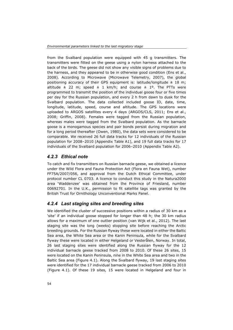
Environmental parameters linked to the last migratory stage
54
from the Svalbard population were equipped with 45 g transmitters. The transmitters were fitted on the geese using a nylon harness attached to the back of the birds. The geese did not show any visible signs of problems due to the harness, and they appeared to be in otherwise good condition (Ens et al., 2008). According to Microwave (Microwave Telemetry, 2007), the global positioning accuracy of their GPS equipment is: latitude/longitude ± 18 m; altitude ± 22 m; speed ± 1 km/h; and course ± 1º. The PTTs were programmed to transmit the position of the individual goose four or five times per day for the Russian population, and every 2 h from dawn to dusk for the Svalbard population. The data collected included goose ID, date, time, longitude, latitude, speed, course and altitude. The GPS locations were uploaded to ARGOS satellites every 4 days (ARGOS/CLS, 2011; Ens et al., 2008; Griffin, 2008). Females were tagged from the Russian population, whereas males were tagged from the Svalbard population. As the barnacle goose is a monogamous species and pair bonds persist during migration and for a long period thereafter (Owen, 1980), the data sets were considered to be comparable. We received 26 full data tracks for 12 individuals of the Russian population for 2008–2010 (Appendix Table A1), and 19 full data tracks for 17 individuals of the Svalbard population for 2006–2010 (Appendix Table A2).
4.2.3 Ethical note
To catch and fix transmitters on Russian barnacle geese, we obtained a licence under the Wild Flora and Fauna Protection Act (Flora en Fauna Wet), number FF75A/2007/056, and approval from the Dutch Ethical Committee, under protocol number CL 0703. A licence to conduct this study in the Natura2000 area ‘Waddenzee’ was obtained from the Province of Friesland, number 00692701. In the U.K., permission to fit satellite tags was granted by the British Trust for Ornithology Unconventional Marks Panel.
4.2.4 Last staging sites and breeding sites
We identified the cluster of successive positions within a radius of 30 km as a ‘site’ if an individual goose stopped for longer than 48 h; the 30 km radius allows for a maximum of one outlier position (van Wijk et al., 2012). The last staging site was the long (weeks) stopping site before reaching the Arctic breeding grounds. For the Russian flyway these were located in either the Baltic Sea area, the White Sea area or the Kanin Peninsula, while for the Svalbard flyway these were located in either Helgeland or Vesterålen, Norway. In total, 26 last staging sites were identified along the Russian flyway for the 12 individual barnacle geese tracked from 2008 to 2010. Of these 26 sites, 15 were located on the Kanin Peninsula, nine in the White Sea area and two in the Baltic Sea area (Figure 4.1). Along the Svalbard flyway, 19 last staging sites were identified for the 17 individual barnacle geese tracked from 2006 to 2010 (Figure 4.1). Of these 19 sites, 15 were located in Helgeland and four in

Chapter 4
55
Vesterålen. The average stopping time at last staging sites for the Russian and Svalbard barnacle geese was 11 and 15 days, respectively (Appendix Figures B1, B2).
Breeding sites were defined as the final stopping site where birds stayed within a radius of 30 km for between 7 and 26 days before the end of June (Kölzsch et al., 2015). In total, 26 breeding sites were recognized along the Russian flyway for the 12 individual barnacle geese tracked from 2008 to 2010, and 19 breeding sites along the Svalbard flyway for the 17 individual barnacle geese tracked from 2006 to 2010 (Figure 4.1).
Some of the Russian barnacle geese that were tracked for more than 1 year have occupied the same staging site from year to year; this was also the case for their breeding sites. Nevertheless, none of the individual Russian barnacle geese arrived at their last staging sites and breeding sites on the same date as in other years (for more information about the last staging and breeding sites of the two populations, see Appendix Tables A1, A2). Departure date was defined as the date on which each individual left its last staging site and headed for its breeding site, and arrival date was defined as the date on which each individual reached its final destination at the breeding site.
4.2.5 Environmental parameters
4.2.5.1 Food availability index
The normalized difference vegetation index (NDVI) is a global vegetation indicator derived by remote sensing and computed as (NIR Red)/(NIR + Red), where NIR and Red are the amount of near-infrared and red light reflectance, respectively, of terrestrial objects (Huete et al., 2002). This index has led to the creation of valuable time series describing the status and phenology of vegetation (Atzberger et al., 2011). The NDVI data we used were derived from NASA’s MODIS Terra satellite at a 1 km spatial resolution and 16-day temporal resolution for 2006–2010. The 23 NDVI images were interpolated to 365 images for each year using linear regression to get a temporal resolution of 1 day rather than the 16-day composite. In the next step, the images were normalized to cover the range 0–100% (Beck et al., 2008). The index obtained, the ‘green wave index (GWI)’, was developed by Shariatinajafabadi et al. (2014). A 0% GWI is used to express the annual minimum NDVI and 100% GWI the annual maximum NDVI for a given pixel. Here we used the 50% GWI (intermediate stage of greenness) as an index of food availability on the arrival date at the breeding sites (Doiron et al., 2013; Shariatinajafabadi et al., 2014). For the departure date from the last staging sites we used actual GWI values as a food availability index.
Barnacle geese mainly forage on red fescue, Festuca rubra, on salt marshes of the Baltic Sea. They also forage on creeping saltmarsh grass, Puccinellia

Environmental parameters linked to the last migratory stage
56
phryganodes, and Hoppner’s sedge, Carex subspathacea, at the Russian breeding sites. Geese in the Baltic Sea area also forage on agricultural fields, mainly on timothy grass, Phleum pratense (van der Graaf et al., 2006). On Norwegian staging sites the geese mainly forage on salt marshes dominated by red fescue, creeping bentgrass, Agrostis stolonifera, and creeping saltmarsh grass and on agricultural land that is mainly being cropped with Phleum spp. and Poa spp. (Prop & Black, 1998). Therefore, we overlaid the GWI image upon a land cover map, and extracted the GWI values from the pixels that were overlaid with grassland, salt marshes and cropland land cover types in a 15 km radius around each staging and breeding site. European Space Agency (ESA)’s 2009 global land cover map was used to define land cover type, which is the finest possible resolution (300 m) global land cover map from Envisat’s Medium Resolution Imaging Spectrometer (http://www.esa.int). To ensure the resolution was the same as GWI images, the land cover map was resampled using the nearest-neighbour algorithm to a resolution of 1 km.
4.2.5.2 Day length (DL)
Day length is the time (h) between sunrise and sunset, and for each individual goose in 2006–2010 it was calculated at the last staging site according to the day of the year (departure date from the last staging site) and latitude of the site using the equations proposed by Kirk (1994). The average day length at the last staging site at the Russian and Svalbard flyways was 21.57 h and 19.96 h, respectively.
4.2.5.3 Weather parameters
In our study we looked at the absolute values of the weather parameters. Although some research shows the significant effect of changes in weather parameters on migration timing (Murphy-Klassen et al., 2005; Žalakevičius, 2000), this kind of research needs a long-term data set of bird migration which we did not have in our study. As weather parameters we used head wind/tail wind, cross wind, mean daily air temperature, low-altitude cloud cover, total precipitation and barometric pressure. All weather parameters were obtained from the European Centre for Medium-Range Weather Forecasts (ECMWF) European Reanalysis (ERA)-interim data calculated every 6 h (0000, 0600, 1200, 1800 hours UTC); the spatial resolution of the data set is 0.75° latitude by 0.75° longitude from 2006 to 2010 (http://www.ecmwf.int). The data closest geographically and temporally to each individual location were extracted. The weather parameters en route for each individual goose were obtained from the GPS points between the last staging and breeding sites while the bird was actively migrating. Since the number of GPS points en route for the Russian barnacle geese varied between two and eight per individual, and for Svalbard barnacle geese between two and 26 per individual, we obtained average values for each of the parameters separately, allowing us to determine

Chapter 4
57
the weather parameters for each individual en route. We did not average the weather parameters for the departure date from the last staging site and arrival date at the breeding sites because we only had one GPS point per individual.
4.2.5.4 Head winds/Tail winds and Cross winds (HW/ TW&CW)
tail wind is one that blows in the direction of flight. It is expressed as a negative value, while a head wind blows opposite to the direction of flight and is expressed as a positive value. A cross wind has a perpendicular component to the direction of flight, with positive values showing wind from the right and negative values wind from the left of the line of flight. Head winds/tail winds and cross winds were determined using the U-wind and V-wind components (wind speed along the X- and Y-axes, respectively) that were calculated every 6 h, beginning at 0000 UTC (EPA, 2000; Hord, 2011; Safi et al., 2013).
Head wind/tail wind and cross winds were obtained from the following equations:
Headwind Tailwind windspeed cos winddirection runway (1)
Crosswind windspeed sin winddirection runway , (2)
where runway is the flight direction.
Wind speed was determined from position components:
Windspeed √ , (3)
where U is the wind speed along the X-axis and V is the wind speed along the Y-axis.
Wind direction was obtained from the following equation:
360/2pi arctan , (4)
again where U is the wind speed along the X- and V is the wind speed along the Y-axis. If U > 0, then wind direction would be 270-Dc, and if U < 0 then wind direction would be 90-Dc.
U and V wind components were extracted from either surface level (10 m above sea level) or different pressure level (1000 hPa, 975 hPa, 950 hPa and 925 hPa) wind direction observations, depending on the altitude of the GPS fix considered. The altitude corresponding to each pressure level was calculated based on its geopotential height, with the closest pressure level to the GPS tag’s altitude being used to extract U- and V-wind components.
4.2.5.5 Mean daily air temperature (MDAT)
Daily air temperatures were obtained for every 6 h beginning at 0000 UTC (0000, 0600, 1200, 1800 UTC) and then averaged to get mean daily air

Environmental parameters linked to the last migratory stage
58
temperature (ºC). As for the wind direction, air temperature data were determined from either surface level (2 m above sea level) or pressure level (1000 hPa, 975 hPa, 950 hPa and 925 hPa) readings, depending on the tag’s altitude.
4.2.5.6 Low-altitude cloud cover (LCC)
Cloud cover at low altitudes (< 2 km above sea level) was determined every 6 h, beginning at 0000 UTC, with values ranging from 0 (no clouds) to 1 (full cloud).
4.2.5.7 Total precipitation (TP)
Total precipitation (mm) refers to any form of water falling from the sky, including snow and rain. Precipitation data were extracted at 3, 6, 9 and 12 h intervals, beginning at 0000 and 1200 UTC. For instance, the total precipitation data at 0600 means the precipitation accumulating between 0000 and 0600. Consequently, to obtain the precipitation accumulating between 0300 and 0600, we subtracted the precipitation at 0300 from the precipitation at 0600. We used the same calculation method to obtain precipitation data for the afternoon and evening; the starting time was 1200.
4.2.5.8 Barometric pressure (BP)
Barometric pressure (atmospheric pressure) is the pressure exerted by the weight of air on the earth’s surface at a specific place and time, and it is determined using the following equation (Berberan-Santos et al., 1997):
/ , (5)
where is barometric pressure (kPa) at flight altitude h (m), is sea level atmospheric pressure (kPa, obtained from ECMWF), m is molar mass of dry air (0.0289644 kg/mol), g is earth surface gravitational acceleration (9.80665 m/s2), h is flight altitude (m), k is the Boltzmann constant (1.3806488(13)×10−23 J/K) and T is sea level temperature (K) which was obtained from ECMWF. Barometric pressure data at the tag’s altitude were obtained for every 6 h, beginning at 0000 UTC.
Chapter 4
59
4.2.6 Statistical analysis
4.2.6.1 Principal component analysis (PCA)
PCA was used to reduce the number of parameters to a few uncorrelated factors, and to avoid multicollinearity in the subsequent multiple regressions (De Lucia & Gottfried, 2011). We used a correlation matrix when doing PCA, since it is always more appropriate when the scale or unit of the measurement differs between variables (McGarigal et al., 2000), as is the case for our parameters. PCA was used to create linearly uncorrelated principal components (PCs) out of the original environmental parameters, thereby reducing the number of dimensions in the data. The number of PCs is equivalent to the number of original parameters; however, the first few PCA-axes encompass most of the variation occurring in the data set, so these can be used to represent the original parameters. The relative importance of the environmental parameters to each PC was examined using the principal component loading. The larger the absolute size of the loading, the more significant that variable is in interpreting the PC (McGarigal et al., 2000). Since there are no accepted ‘absolute’ standards for the cutoffs, we decided to use a cutoff of |0.45|in our study, following the benchmark proposed by Tabachnick and Fidell (2001). The PCA for the last staging sites was calculated using eight continuous environmental parameters that included GWI, day length, head wind/tail wind, cross wind, mean daily air temperature, low-altitude cloud cover, total precipitation and barometric pressure. Of the eight environmental parameters, we chose seven, including GWI, head wind/tail wind, cross wind, mean daily air temperature, low-altitude cloud cover, total precipitation and barometric pressure, for computing the PCA at the breeding sites. Moreover, six weather parameters comprising head wind/tail wind, cross wind, mean daily air temperature, low-altitude cloud cover, total precipitation and barometric pressure, were used to compute the PCA en route. At the breeding sites we did not consider day length because of the 24 h daylight regime at that time of year at those latitudes. The environmental parameters en route were extracted only for the active flight period. This is especially important for the Svalbard barnacle goose because it has to make a nonstop flight over the sea. Therefore, the parameters en route comprised only the weather variables and did not include GWI and day length.
4.2.6.2 Linear mixed-effects model
We combined the mixed-effect linear regression method and PCA to investigate the relationship between the last stage of barnacle goose spring migration timing and the environmental parameters. Linear mixed-effect modelling was used to avoid pseudoreplication caused by sequential observations of individual geese. The individual identity (ID) and tracking year were considered as random effects, and those principal components with an eigenvalue >1 (Quinn

Environmental parameters linked to the last migratory stage
60
& Keough, 2002) were used as fixed effects. Backward elimination of statistically nonsignificant fixed effects (P > 0.05) was used to define a model that adequately described the data, while the random effects were always kept in the model. However, the random effects with zero variance were removed from the model before running the backward elimination (Mathworks, 2013). For the fixed effects, P values were calculated for an F test based on the Satterthwaite approximation, and P values for random effects were calculated based on the likelihood ratio test. All analyses were performed on the ‘lmer’ object of the ‘lme4’ (Bates et al., 2014) and ‘lmerTest’ packages (Kuznetsova et al., 2014) in R version 3.1.2 (R Core Team, 2014). Pearson correlation (r) was used to measure the positive (delay) or negative (acceleration) impact of the significant PCs on the departure and arrival dates. The proportion of residual variance in the mixed model that was due to the individual barnacle geese and year (i.e. repeatability) was calculated by dividing the proportion of variance explained by the random effect by the total variance (Lessells & Boag, 1987).
4.2.6.3 Predictability
To check whether the geese are able to rely on certain environmental parameters at their last staging site as indicators for predicting the situation at their breeding areas, we tested the relationship between arrival date at the breeding site with the PCs (eigenvalue >1) of the environmental parameters at the last staging site, and the relationship between departure date from the last staging site with the PCs of environmental parameters at the breeding site using linear mixed-effect analysis. We used Pearson correlation (r) to examine the correlation between environmental parameters at the last staging site and breeding sites.
4.3 Results The results of the PCA are shown in Table 4.1 for the Russian and Table 4.2 for the Svalbard populations. The random (ID, year) and fixed effects (selected PCs) were analysed with regard to departure date from the last staging site and arrival date at breeding sites (Tables 4.3 and 4.4 for the Russian and Svalbard population, respectively). The key environmental parameters relating to goose migration along the Svalbard and Russian flyways are summarized in Table 4.5. The results of PCA and linear mixed-effect regression for the last staging site, en route and breeding site are given in more detail below.
For the Svalbard barnacle geese, only two individuals were tracked for more than one year; therefore, we only calculated the repeatability for the Russian population. Our results showed repeatable inter-individual and between-year differences in arrival/departure date for the Russian barnacle geese. This

Chapter 4
61
showed the percentage of the residual variance in arrival/departure date, not accounted for by the fixed effects (see Appendix Table A3).
4.3.1 Last staging site
For the Russian (Table 4.1) and Svalbard (Table 4.2) populations, the first three PCs with eigenvalues > 1 accounted for 65.7% and 64.3% of the total variance of environmental parameters at the last staging site, respectively.
The result of linear mixed-effect regression using these three PCs showed that for the Russian population PC1lsR was a significant factor on departure date from the last staging site (Table 4.3). Pearson correlation showed that departure date was delayed for PC1lsR (r24=0.67). Mean daily air temperature and barometric pressure showed the highest negative and day length and low-altitude cloud cover the highest positive correlations with PC1lsR scores (factor loadings of MDAT, BP, DL and LCC: R=-0.89, -0.78, 0.77 and 0.73, respectively).
For the Svalbard population, linear mixed-effect regression showed that departure date was significantly influenced by the second PC (Table 4.4). However, PC1lsS, which contains the largest variance (27.8% of the overall variance), was not selected by the linear mixed-effect regression model. PC2lsS accelerated (r17=-0.68) departure dates. GWI and day length provided the major negative loading on PC2lsS (GWI: R=-0.96; DL: R=-0.49).
4.3.2 En route
Of the six PCs en route only the first three were used in linear mixed-effect regression; they explained 77.9% and 77.8% of total variation of parameters in PCA en route for the Russian (Table 4.1) and Svalbard (Table 4.2) populations, respectively.
Linear mixed-effect regression analysis showed that arrival date at the Russian breeding site was significantly related to the PC2eR (Table 4.3). Arrival date was delayed by PC2eR (r24=0.27). Low-altitude cloud cover and barometric pressure provided the major loading on that PC (LCC: R=0.81; BP: R=-0.78).
In the regression model, only PC3eS made a significant contribution to arrival date at the Svalbard breeding site (Table 4.4). Although the information content of the cumulative variance of PC1eS and PC2eS (61%) is higher than that of PC3eS (16.8%), they were not selected as significant factors by the model. PC3eS delayed the arrival date at the breeding site (r17=0.48) and it had positive loadings on mean daily air temperature (MDAT: R=0.83) and low-altitude cloud cover (LCC: R=0.53).

Environmental parameters linked to the last migratory stage
62
4.3.3 Breeding site
The first three PCs accounted for 75.8% and 67.3% of the total variation in the matrix of environmental parameters at the Russian (Table 4.1) and Svalbard (Table 4.2) breeding sites, respectively. These PCs were used in the linear mixed-effect regression analysis to determine the most significant PCs for arrival date at the breeding site.
The results of this analysis indicated a significant relationship between arrival date at the Russian breeding site and PC2bR (Table 4.3). Arrival date was delayed by PC2bR (r24=0.68). It was positively loaded on GWI (R=0.83) and negatively on mean daily air temperature (R=-0.72).
For the Svalbard population there was a significant relationship between PC1bS and PC3bs with arrival date at the Svalbard breeding site (Table 4.4). Although PC3bs was significantly related to arrival date, the correlation between them was extremely low (r17=-0.06). Therefore, we did not interpret the result for this PC. PC1bS accelerated the arrival at the Svalbard breeding site (r17=-0.51). GWI and low-altitude cloud cover showed highly negative correlations with PC1bS (factor loading of GWI and LCC: R=-0.70 and -0.78, respectively), and head wind/tail wind showed a highly positive correlation with this PC (factor loading of HW/TW: R=0.74). PC1bS had a lower negative correlation with mean daily air temperature (R=-0.53).
Table 4.1. Eigenvalues and variances of the first three principal components (eigenvalue>1) of the PCA conducted on the environmental parameters matrix, with corresponding factor loadings of the parameters for the last staging site (PClsR), en route (PCeR) and breeding site (PCbR) of the Russian barnacle goose population.
Envir. Par.
Last staging site En route Breeding site
PC1lsR PC2lsR PC3lsR PC1eR PC2eR PC3eR PC1bR PC2bR PC3bR
GWI -0.31 -0.75 -0.29 Nc Nc Nc -0.38 0.83 0.14 DL 0.77 -0.13 -0.09 Nc Nc Nc Nc Nc Nc HW/TW -0.05 -0.26 -0.74 -0.46 -0.17 0.72 -0.24 -0.32 -0.76 CW -0.28 0.34 -0.56 0.46 0.15 0.66 -0.63 -0.13 -0.45 MDAT -0.89 -0.22 0.14 0.84 -0.38 -0.15 0.50 -0.72 -0.05 LCC 0.73 -0.09 -0.23 -0.37 0.81 -0.08 -0.83 -0.27 0.13 TP 0.18 -0.76 0.30 0.79 0.22 0.14 -0.07 -0.33 0.85 BP -0.78 0.06 -0.03 -0.37 -0.78 -0.01 0.68 0.40 -0.33 EEVA 2.72 1.41 1.11 2.37 1.24 1.05 1.99 1.65 1.64
Var (%) 34.1 17.6 14.0 39.5 20.8 17.6 28.5 23.7 23.6 Cum. Var (%)
34.1 51.7 65.7 39.5 60.3 77.9 28.5 52.2 75.8
Loadings >|0.45| are in bold type. GWI: green wave index; DL: day length; HW/TW: headwind/tail wind; CW: cross wind; MDAT: mean daily air temperature; LCC: low-altitude cloud cover; TP: total precipitation; BP: barometric pressure; EEVA: Eigenvalue; Var: Variance; Cum. Var: Cumulative Variance; 'Nc': parameter that was not considered in the PCA.

Chapter 4
63
Table 4.2. Eigenvalues and variances of the first three principal components (eigenvalue>1) of the PCA conducted on the environmental parameters matrix, with corresponding factor loadings of the parameters for the last staging site (PClsS), en route (PCeS) and breeding site (PCbS) of the Svalbard barnacle goose population.
Envir. Par.
Last staging site En
route Breeding site
PC1lsS PC2lsS PC3lsS PC1eS PC2eS PC3eS PC1bS PC2bS PC3bS
GWI -0.04 -0.96 -0.14 Nc Nc Nc -0.70 -0.09 -0.47 DL 0.07 -0.49 0.63 Nc Nc Nc Nc Nc Nc HW/TW 0.60 -0.24 0.37 0.88 0.07 0.08 0.74 0.04 0.05 CW -0.80 0.05 0.31 -0.13 0.74 -0.08 0.45 -0.33 0.51 MDAT -0.50 -0.45 -0.67 -0.03 -0.43 0.83 -0.53 0.52 0.57 LCC 0.16 -0.33 0.23 -0.02 0.72 0.53 -0.78 -0.14 0.40 TP 0.61 -0.15 -0.34 -0.90 0.10 0.15 -0.28 -0.65 -0.14 BP -0.76 -0.14 0.25 0.88 0.15 0.10 0.06 0.77 -0.27 EEVA 2.22 1.58 1.33 2.37 1.28 1.01 2.21 1.43 1.06
Var (%) 27.8 19.8 16.7 39.6 21.4 16.8 31.6 20.5 15.2 Cum. Var (%) 27.8 47.6 64.3 39.6 61.0 77.8 31.6 52.1 67.3
Loadings >|0.45| are in bold type. GWI: green wave index; DL: day length; HW/TW: headwind/tail wind; CW: cross wind; MDAT: mean daily air temperature; LCC: low-altitude cloud cover; TP: total precipitation; BP: barometric pressure; EEVA: Eigenvalue; Var: Variance; Cum. Var: Cumulative Variance; 'Nc': parameter that was not considered in the PCA. Table 4.3. Results of the mixed model after running backward elimination to remove nonsignificant fixed effects (principal components of the environmental parameters) on departure date from last staging sites and arrival date at breeding sites for 12 individual GPS-tagged Russian barnacle geese (2008–2010).
Migration timing
Rand. effect Var. χ2 P Fixed
effect
Sum of squares error
F P
Dep.from last staging site
ID 8.06 2.38 0.12 PC1lsR 202.08 20.98 < 0.001 Year 2.99 0.94 0.33 PC2lsR 11.33 1.02 0.32 Resid. 11.67 PC3lsR 4.05 0.34 0.56
Arr. at breeding site
ID 4.32 0.73 0.39 PC1eR 27.69 2.20 0.15 Year 18.50 4.53 0.03 PC2eR 49.32 4.61 <0.05 Resid. 12.76 PC3eR 6.11 0.47 0.49 Year 12.81 5.77 0.01 PC1bR 28.57 2.27 0.14 Resid.l 13.05 PC2bR 221.47 16.89 < 0.001 PC3bR 1.72 0.13 0.71
Random effects with zero variance were removed from the models before running backward elimination. PClsR: PCs obtained from eight environmental parameters at the last staging sites; PCeR: PCs obtained from six environmental parameters en route; PCbR: PCs obtained from seven environmental parameters at breeding sites.

Environmental parameters linked to the last migratory stage
64
Table 4.4. Results of the mixed model after running backward elimination to remove nonsignificant fixed effects (principal components of the environmental parameters) on departure date from last staging sites and arrival date at breeding sites for 17 individual GPS-tagged Svalbard barnacle geese (2006–2010)
Migration timing
Rand. effect Var. χ2 P Fixed
effect
Sum of squares error
F P
Dep. from last staging site
Year 40.50 2.91 0.08 PC1lsS 0.009 0.004 0.98 Resid. 26.98 PC2lsS 965.36 36.86 < 0.001 PC3lsS 68.50 2.66 0.12
Arr. at breeding site
ID 26.73 0.06 0.80 PC1eS 35.66 0.38 0.56 Year 60.04 1.28 0.25 PC2eS 70.89 0.82 0.38 Resid. 92.61 PC3eS 659.47 6.09 < 0.05 ID 151 2.26 0.13 PC1bS 24.61 5674965 <0.001 Resid. 0.00 PC2bS 0.00 0.17 0.68 PC3bS 0.45 105775 <0.001
Random effects with zero variance were removed from the models before running backward elimination. PClsR: PCs obtained from eight environmental parameters at the last staging sites; PCeR: PCs obtained from six environmental parameters en route; PCbR: PCs obtained from seven environmental parameters at breeding sites. Table 4.5. A summary of the significant principal components (P < 0.05) relating to migration timing at the last staging site, en route and breeding site in the Russian and Svalbard flyways. PCs
(P < 0.05)
Environmental parametersFlyway Migration
timing GWI DL HW/TW CW MDAT LCC TP BP
Russian
Dep. from last staging site
PC1lsR + +
Arr. at breeding site
PC2eR Nc Nc +
PC2bR + Nc
Svalbard
Dep. from last staging site
PC2lsS + +
Arr. at breeding site
PC3eS Nc Nc + +
PC1bS + Nc + +
GWI: green wave index; DL: day length; HW/TW: headwind/tail wind; CW: cross wind; MDAT: mean daily air temperature; LCC: low-altitude cloud cover; TP: total precipitation; BP: barometric pressure; ‘+’: parameters with high loading values on the significant PCs that delayed migration timing; ‘-’: parameters with high loading values on the significant PCs that accelerated the migration timing; ‘Nc’: parameter that was not considered in the PCA. Delayed (‘+’) or accelerated (‘-’) effect on migration timing is based on the correlation of the significant PCs with migration timing and the sign of loading values on those PCs.

Chapter 4
65
4.3.4 Predictability
Departure date from the last staging site along the Russian flyway was significantly related to – and delayed (r24=0.44) by – PC2bR. However, for the Svalbard population there was no significant relationship between departure date from the last staging site and the principal components of the environmental parameters at breeding sites (Table 4.6).
The results of linear mixed-effect regression indicated that for both populations the same PCs of the environmental parameters at the last staging site were related to departure date from that site (Table 4.3 and 4.4), as well as arrival date at breeding sites (Table 4.7). The only exception was PC3lsS that was significantly related to arrival date at the breeding site, but was not related to departure date from the last staging site on the Svalbard flyway. For the Russian population, PC1lsR was significantly related to arrival date at the breeding site (Table 4.7): the arrival date was delayed with PC1lsR (r24=0.51). Arrival date at the Svalbard breeding site was significantly influenced by PC2lsS and PC3lsS (Table 4.7). PC2lsS accelerated (r17=-0.61) and PC3lsS delayed (r17=0.25) arrival date.
We did not find a significant relationship between weather parameters for the last staging site and breeding sites. We only found a significant relationship between cross winds at the last staging site and barometric pressure at breeding sites on the Russian flyway, and between mean daily air temperature at the last staging site and barometric pressure at breeding sites on the Svalbard flyway (Table 4.8).
Table 4.6. Results of the mixed model after running backward elimination to remove nonsignificant fixed effects (principal components of the environmental parameters at the breeding site) on departure date from last staging sites for 12 individual GPS-tagged Russian (2008–2010) and 17 individual GPS-tagged Svalbard barnacle geese (2006–2010).
Migration timing
Rand. effect Var χ2 P Fixed
effect
Sum of squares error
F P
Dep. from the last staging site in the Russian flyway
ID 10.99 1.99 0.15 PC1bR 41.35 2.66 0.11 Year 8.67 3.31 0.06 PC2bR 72.05 4.61 <0.05 Resid. 16.2 PC3bR 9.72 0.60 0.45
Dep. from the last staging site in the Svalbard flyway
ID 87.66 0.66 0.41 PC1bS 293.35 2.83 0.11 Year 10.28 0.39 0.53 PC2bS 119.54 1.15 0.29
Resid. 11.86 PC3bS 20.01 0.19 0.66
Random effects with zero variance were removed from the models before running backward elimination. PCbR: PCs obtained from seven environmental parameters at the breeding sites in the Russian flyway; PCbS: PCs obtained from seven environmental parameters at the breeding sites in the Svalbard flyway.

Environmental parameters linked to the last migratory stage
66
Table 4.7. Results of the mixed model after running backward elimination to remove nonsignificant fixed effects (principal components of the environmental parameters at the last staging site) on arrival date at the breeding sites for 12 individual GPS-tagged Russian (2008–2010) and 17 individual GPS-tagged Svalbard barnacle geese (2006–2010). Migration timing Rand. Var. χ2 P Fixed
effect
Sum of square error
F P
Arr. at the Russian breeding site
ID 11.07 4.60 0.03 PC1lsR 51.18 5.55 <0.05 Year 22.90
6.84 0.00 PC2lsR 2.59 0.29 0.59
Resid. 8.86 PC3lsR 10.16 1.22 0.28
Arr. at the Svalbard breeding site
ID 113 5.01 0.02 PC1lsS 0.00 1.91 0.66 Resid. 0.00
PC2lsS 23.66 6439394 <0.001
PC3lsS 3.16 861660 <0.001 Random effects with zero variance were removed from the models before running backward elimination. PClsR: PCs obtained from eight environmental parameters at the last staging sites in the Russian flyway; PClsS: PCs obtained from eight environmental parameters at the last staging sites in the Svalbard flyway. Table 4.8. Correlation matrix displaying Pearson correlation coefficients of the environmental parameters at the last staging site and breeding sites.
Flyway Breeding site GWI HW/TW CW MDAT LCC TP BP
Last staging site
Russia
GWI -0.14 -0.02 0.10 0.28 0.13 -0.10 -0.03
HW/TW -0.06 -0.27 -0.15 -0.09 -0.02 0.15 -0.02 CW -0.26 0.20 0.27 0.16 0.36 0.15 -0.39* MDAT -0.33 0.09 0.07 0.12 -0.05 0.02 -0.02
LCC 0.35 0.29 -0.02 -0.11 -0.004 -0.19 0.11
TP 0.07 -0.29 0.06 0.11 -0.05 -0.11 0.26
BP -0.18 -0.04 0.00 0.14 -0.06 -0.18 0.05
Svalbard
GWI 0.25 -0.36 -0.20 -0.03 0.04 0.03 -0.27
HW/TW 0.20 -0.04 -0.40 0.30 0.33 0.26 -0.10
CW 0.09 -0.01 0.03 0.05 -0.21 -0.29 -0.06
MDAT -0.12 -0.13 0.19 -0.24 0.12 -0.10 -0.47*
LCC 0.30 -0.16 -0.21 0.22 0.10 0.00 0.14
TP 0.14 -0.17 -0.11 -0.16 0.01 0.30 0.06
BP 0.03 0.18 0.06 -0.07 -0.08 -0.37 -0.10 GWI: green wave index; HW/TW: headwind/tail wind; CW: crosswind; MDAT: mean daily air temperature; LCC: low-altitude cloud cover; TP: total precipitation; BP: barometric pressure. Asterisk indicates significance of correlation: *P < 0.05.
Chapter 4
67
4.4 Discussion Our results reveal the importance of environmental parameters at the last stage of migration on the date of departure of individual barnacle geese from their last staging site and their arrival date at their breeding sites along two flyways. More precisely, we found that departure date from the last staging site on the Russian flyway was related to day length, mean daily air temperature, low-altitude cloud cover and barometric pressure (PC1lsR in our analysis) and on the Svalbard flyway to GWI and day length (PC2lsS). The main en route parameters that were related to arrival date at the breeding sites comprised low-altitude cloud cover and barometric pressure (PC2eR) for the Russian flyway and mean daily air temperature and low-altitude cloud cover (PC3eS) for the Svalbard flyway. From the parameters at the breeding sites we found GWI and mean daily air temperature (PC2bR) to be important for the arrival date at Russian breeding sites, and GWI, head wind/tail wind, mean daily air temperature and low-altitude cloud cover (PC1bS) for the arrival date at Svalbard breeding sites.
4.4.1 Last staging site
Considering the correlation of day length, mean daily air temperature, low-altitude cloud cover and barometric pressure with PC1lsR, along with the fact that PC1lsR delayed departure date, we can say the Russian geese departed from their last staging site earlier when barometric pressure and mean daily air temperature were higher, but day length and cloudiness was lower. Reliance on day length towards the end of the journey and departure on a fixed date was also found to be important for the spring migration of pink-footed geese (Duriez et al., 2009). Furthermore, it seems visibility could be an important parameter affecting departure, since high temperatures and high barometric pressures are associated with clear skies (Kaiser, 2000). For northern wheatears, Oenanthe oenanthe, the majority of stays during spring migration coincided with an almost completely overcast sky: the cloud cover was significantly greater for birds that remained at sites than for birds that departed (Dierschke & Delingat, 2001).
Our results showed that PC2lsR and PC3lsR were not significant factors affecting departure date. PC2lsR was mainly related to GWI and precipitation. This result is in contrast to what we expected, because based on the deposition rate hypothesis we expected that GWI would be related to departure dates of the Russian barnacle geese. The reason for this unexpected result might be related to the fuel expenditure during the flight between the last staging site and their breeding sites. Some of the Russian barnacle geese made a short stop of 2–4 days between their last staging site and their breeding site, which may have given them enough time to refuel. In other words, instead of making one long flight with a large fuel load, they made shorter flights with smaller fuel loads,

Environmental parameters linked to the last migratory stage
68
which reduces total energy costs for the migration and increases energy savings (Green et al., 2002). The Russian geese may also build up their energy reserves beforehand by staying longer in the White Sea area or along the Baltic coast. Even though many bird species take action to avoid rain (Hume, 1986), our results did not show much effect of rainfall on the geese.
Since PC3lsR was mainly related to wind conditions, we conclude that wind conditions at the last staging site have no prominent effect on departure decisions of Russian barnacle geese. Kölzsch et al. (2016) observed that the selection of supportive winds was stronger in autumn than spring because the general wind conditions were favourable between western Europe and the Russian Arctic during spring. However, our conclusion is in contrast with other studies, which have emphasized the importance of wind conditions on migration timing (e.g. Erni et al., 2005; Pulido, 2007b).
Departure date from the last staging site on the Svalbard flyway was not related to the PC1lsS, although it accounted for the largest variance of the data. PC1lsS was mainly related to wind, temperature, precipitation and barometric pressure. As we observed for the Russian barnacle geese, rainfall did not have much effect on departure date for the Svalbard barnacle geese.
Our results highlighted the impact of GWI and day length (PC2lsS) on departure decision making by the Svalbard barnacle geese. However, GWI may play the major role because it had a higher loading on PC2lsS than day length. Bauer et al. (2006) also found that food quantity and quality had a crucial impact on departure and staging decisions at the last stage of migration for Arctic-breeding migratory geese. Our result is in line with the deposition rate hypothesis, which suggests that deteriorating foraging conditions trigger migration. Prop et al. (2003) came to a similar conclusion about the decision making by barnacle geese for leaving their last staging sites in Norway. Moreover, Duriez et al. (2009) suggested that using day length to make departure decisions from northern Norway is the best strategy for the geese since there is a weak correlation between weather conditions in Norway and Svalbard.
4.4.2 En route
Considering the relation of PC2eR to arrival date, and the correlation of the parameters with high loading on this PC (i.e. barometric pressure and cloudiness), we may conclude that higher barometric pressure and less cloudiness en route along the Russian flyway were related to earlier arrival at the final destination. However, less cloudiness may be just an indirect effect of higher barometric pressure (Kaiser, 2000). This supports the hypothesis that visibility is an important parameter in the orientation of migrating birds (Åkesson & Bäckman, 1999).

Chapter 4
69
We found that wind conditions (head wind/tail wind and cross wind) en route were not related to the migration timing of the individual Russian and Svalbard geese, which is opposite to previous studies (Erni et al., 2005; Liechti, 2006; Pulido, 2007b). Wind parameters en route at the Russian flyway had high loading on PC3eR, but this PC was not selected by the model. Also, arrival date at Svalbard breeding sites was not related to PC1eS and PC2eS, although these first two PCs accounted for 61% of the total variance in the data. As Table 4.2 shows, wind parameters had the highest correlation with PC1eS and PC2eS.
The flight altitude of the geese en route might be why wind parameters were not related to arrival date. For the Russian and Svalbard geese, 60% and 50% of flights were at altitudes less than 5 m above sea level, respectively. As Finn et al. (2012) noted, birds fly close to water surfaces for two reasons: (1) to avoid head winds and (2) to take advantage of ground effects. They found that the wind speeds decline at heights below 4 m, so birds might be expected to fly lower when flying in headwind. Moreover, birds that fly close enough to water surface may also benefit energetically by use of ground effect (Finn et al., 2012). Ground effects can be caused by an interaction between the bird’s wings and the ground or water surface that increases lift, thus minimizing power needed to stay aloft and maximizing range (De la Cueva & Blake, 1993). In other words, lower wind speeds plus ground effects can minimize energy expenditure during flight (Finn et al., 2012).
However, the effect of wind on the Svalbard geese may be less, because they could compensate for unfavourable wind conditions en route by changing flight altitude and choosing the best flight direction. On the other hand, for reasons of safety, the Russian barnacle geese may not be able to fly low over land, so they could not totally compensate for unfavourable wind conditions by changing flight altitude. This could be why about 90% of their low flights were over sea, and 78% of the high flights were over land.
Precipitation also had a high loading on PC1eS. Like departure date from the last staging site, rainfall en route was not related to migration timing and therefore did not delay or accelerate arrival date at breeding sites. Our results show that arrival date at the Svalbard breeding sites was related to PC3eS, and this was loaded on mean daily air temperature and cloud cover. We found that lower temperatures and less cloudiness en route were related to geese arriving earlier at their Svalbard breeding sites.
4.4.3 Breeding site
Our results indicated that PC2bR was mainly related to arrival date at Russian breeding sites and this was highly loaded by GWI and temperature. These two parameters had the highest correlation with PC2bR among the first three PCs of the environmental parameters at the breeding site (Table 4.1). The arrival date is such that the growth of goslings is synchronized with high levels of food

Environmental parameters linked to the last migratory stage
70
availability (Owen, 1980). Using ground data, van der Graaf et al. (2006) and van Der Jeugd et al. (2009) found that barnacle geese arrive at their Russian breeding sites before the peak in nutrient biomass. So the geese may follow the early settling strategy that allows the goslings to benefit from high-quality food and have enough time for pre-migratory fattening (Prop & de Vries, 1993).
Moreover, temperature at the breeding site may have indirect effects on arrival date, via its influence on food availability. Indeed, arrival date and timing of nesting of these geese is highly constrained by the food availability, which is dependent on the degree of snow cover (Fox et al., 2006; Madsen et al., 2007; Prop & de Vries, 1993). In other words, food availability is related to the rate of snow melt, which starts when the air temperature rises above 0º C (Kostin & Mooij, 1995). As a consequence, birds arriving early have to graze on low-quality feed and must wait until more nutritious plant resources become available. However, the costs of early arrival can be offset by a better survival rate for goslings hatching early in the season, because they benefit from the longest availability of high-quality food (Prop & de Vries, 1993). Therefore, the temporal variability of food at the breeding site affects the costs and benefits of arrival date in terms of food acquisition (Fox et al., 2006). Because of this, there is a possibility that, over time, Arctic-nesting geese that arrive too late with respect to rapid seasonal developments (as a consequence of climate change and global warming) will miss the optimal breeding conditions.
Russian barnacle geese that arrive earlier at their breeding sites face higher air temperatures. As the results of Smith III and Hayden (1984) showed, spring migration phenology may be related to large-scale atmospheric circulation patterns. High temperatures may be an indirect effect of other environmental parameters associated with weather systems, such as, for example, barometric pressure and/or favourable winds. During the passage of a low pressure system from the Atlantic, large-scale changes in temperature, pressure and wind conditions occur. The geese may be able to detect these conditions of low pressure systems, which may give them an extra boost on their way towards their destination (Smith III & Hayden, 1984). In other words, the arrival of geese at their Arctic breeding sites is associated with strong southerly winds and these winds at higher latitudes are generally associated with low-pressure systems. The geese fly on the appropriate side of low-pressure systems to obtain a tail wind, thus increasing their flight speeds (Ball, 1983). It has been suggested that migratory birds may be sensitive to changes in weather patterns coinciding with the start of spring and so adjust their spring migration according to weather conditions in central and northern latitudes. Time of arrival at the breeding site could, therefore, be an indicator of spring weather conditions, and any change in arrival date occurring over a long period may be reflecting changes in those conditions (Ball, 1983).

Chapter 4
71
Arrival date at Svalbard breeding sites was mainly related to PC1bS. GWI, low-altitude cloud cover and head wind/tail wind had high component loading values for PC1bS, whereas temperature had a lower loading. With the explanation just given above in mind regarding the relation between food and temperature, we can say PC1bS corresponds to food availability at the breeding site. Moreover, it is likely that PC1bS also reflects the importance of visibility for arrival date at the breeding site, since cloudiness and head winds can both be related to visibility. Cloudiness at the breeding site had a direct effect on arrival date. Moreover, we found that Svalbard geese arrived earlier at their breeding sites with increasing head winds. Since the geese are flying north, head winds (winds coming from the north) near their point of arrival make it likely that the landing site is more sheltered, with possibly better visibility.
4.4.4 Repeatable inter-individual and between-year variation in migration timing
We observed inter-individual and between-year variability in migration timing for the Russian barnacle geese. This could be because of a trade-off between staying longer at the last staging site to accumulate a larger body store and early arrival at the breeding site to increase the survival rate of the offspring (Prop et al., 2003). Repeatable variation in arrival dates at the breeding site has been observed for other migratory geese such as snow geese, Anser caerulescens (Bety et al., 2004). Migration timing of birds may have a genetic basis (Berthold et al., 2001) as was suggested for snow geese (Bety et al., 2004). This genetic basis for migration timing may consequently also explain the inter-individual variation in migration timing for the Russian barnacle geese. Moreover, phenotypic plasticity, which is an environmentally based change in the phenotype, could also explain some of the observed variability in migration timing (Teplitsky et al., 2008).
4.4.5 Predictability
For both geese populations, the same combination of environmental parameters (i.e. the same PCs) at the last staging site were related to both departure date from this site and arrival at the breeding site. Moreover, the same PCs of the environmental parameters at the Russian breeding site that were significantly related to arrival at this site were also related to departure from the last staging site. However, this does not mean that environmental parameters at the last staging site were indicators for the geese of conditions at their breeding site. This is especially true for Svalbard barnacle geese, since we did not find any significant relationship between the PCs of the environmental parameters at the breeding site and departure from the last staging site. In fact, having the same combination of environmental parameters at the last staging or breeding site relating to date of departure or arrival might be linked to the high correlation between arrival date at the

Environmental parameters linked to the last migratory stage
72
breeding site and departure date from the last staging site for the Russian (r24=0.69, P < 0.001) and Svalbard (r17=0.87, P < 0.001) populations. Moreover, we did not find a significant relationship between environmental parameters at the last staging sites and breeding sites on both flyways. Tombre et al. (2008) found that successive sites on the Svalbard flyway were not climatically linked, so barnacle geese could not use conditions at one site to predict conditions they might encounter at the next. Moreover, Hahn et al. (2011) have indicated that climatic conditions on Svalbard breeding sites were not predictable from climatic conditions on Norwegian staging sites. They found no correlation between temperature and snow conditions on the departure date of pink-footed geese in May from their mid-Norwegian staging site and conditions actually occurring (in May) on Svalbard breeding sites. They only found a weak correlation between temperature in May on northern Norwegian staging sites and temperature and snow conditions on breeding sites in the Svalbard archipelago. Nevertheless, Kölzsch et al. (2015) believed that individual barnacle geese are able to predict foraging conditions at subsequent staging sites since the dates of spring onset were correlated between consecutive sites.
Lower predictability between the last staging and breeding sites may cause barnacle geese to rely more on time-related cues such as day length and departure on a fixed date, as suggested by van der Graaf (2006). Therefore, with climate change and an earlier onset of spring (IPCC, 2007), geese may arrive later at the breeding site with respect to the start of spring there. This could lead to an increase in nesting success due to a longer frost- and snow-free season on the Arctic breeding site (Jensen et al., 2014; Madsen et al., 2007). On the other hand, the advancement of the growth of forage plants, due to earlier melting of snow, may lead to a mismatch between the gosling’s time of hatching and the time of peak plant nutrient content. This could ultimately impact the growth and survival of goslings because they have to ingest feed of lower quality (Gauthier et al., 2013).
4.5 Conclusion Our results showed that the environmental parameters at the last stage of migration have a considerable correlation with arrival date at the breeding site. More knowledge about the parameters and decision rules used by birds during migration is essential to be able to predict the consequences of environmental changes for them (Bauer et al., 2011). Since migratory birds depend on forage of high nutritional quality, they have to follow the advancement of plant phenology. An inappropriate arrival date at the breeding site can be disadvantageous for Arctic-breeding geese (Brown & Brown, 2000; Madsen et al., 2007). Barnacle geese may benefit from using the local environmental conditions to adjust their migration timing; however, they may not be able to predict the situation at their destination from their last staging site. We found

Chapter 4
73
weather parameters to have a significant impact on migration timing. For instance, earlier departure from the last staging site or earlier arrival at the breeding site were related to lower cloudiness and therefore higher visibility along the flyway. Some weather parameters could also indirectly be related to migration timing, such as high temperatures and high barometric pressures, which are associated with clear skies.
We observed some differences between the Russian and Svalbard flyways with respect to the effect of environmental parameters on migration timing. For instance, food availability was not an important parameter for departure date from the last staging site for the Russian barnacle geese, whereas it was for the Svalbard geese. The latter, which fly over large stretches of sea, do not have the opportunity to feed, drink or rest as the Russian geese flying over land do. Moreover, the distance between the last staging site and breeding sites is different for each population, which may have an effect on which environmental parameters are used as cues for departure.
Besides environmental parameters such as day length, weather and food, the physical condition (body fat) of the geese may be an endogenous parameter affecting migration timing. Differences in physical condition may influence arrival date and reproductive success of migratory birds (Norris et al., 2004). Schaub et al. (2008) have shown that some individual birds that put on fat at a higher rate leave their current site earlier than others. However, we had no access to this information and could not incorporate this parameter into our analysis. Integrating environmental parameters (food, weather and day length) with energy cues could be used to build an optimal migration model so as to be able to more accurately predict migration timing of avian herbivores.

Environmental parameters linked to the last migratory stage
74

75
Chapter 5 Predicting the stopover selection of barnacle geese using expert system1
1 This chapter is based on: Shariati Najafabadia, M., Skidmore, A.K., Darvishzadeh, R., Exo, k.M, Nolet, B.A., Kölzsch, A., Griffin, L., Stahl, J., Cabot, Toxopeus, A.G., Predicting the stopover selection of barnacle geese using expert system. In review: Ecological Modelling.
Stopover site selection
76
Abstract
The study of stopover sites has received a lot of attention in avian ecology, being especially important for many long-distance migrants, some of which have to pause several times during migration. The survival of many migratory birds depends primarily on food availability at these stopovers. However, previous studies show that there is a lack of knowledge about site selection where migratory birds stop to refuel energy stores. In the present study, a Bayesian expert system has been used to incorporate environmental parameters, to determine their relationship with the presence of barnacle geese at stopover sites. Data on stopover sites was obtained from satellite-tracked barnacle geese (Branta leucopsis) for three different breeding populations in the Western Palearctic (i.e. Russian, Svalbard and Greenland). The results from the present study showed that the posterior probability of presence at the stopover sites obtained from the Bayesian model was close to one and significantly higher than the posterior probability of absence. Therefore, the Bayesian expert system detected the stopover sites of the geese correctly and can be used as a proper method for modelling the presence/absence of barnacle geese at the stopover sites in the future. This study introduces a new method into movement ecology to identify and predict the importance of the different environmental parameters for stopover site selection by migratory geese. This is particularly important from both a conservation and an agro-economic point of view with the goal of reducing possible conflicts between geese and agricultural interests.

Chapter 5
77
5.1 Introduction Stopovers are places along a migration route where birds mostly rest and forage to replenish energy reserves before continuing their journeys (Newton, 2008). This is a common behavioural strategy among most migratory animals and in particular, those using active movement (e.g. flapping flight in birds) because they often are unable to store enough energy to complete their migration without periods of foraging (Hedenström & Alerstam, 1997).
Having such breaks during migration is especially important for Arctic-nesting geese as many of them are partial capital breeders and may bring body stores to the breeding grounds, in order to survive initial adverse conditions and produce a clutch of eggs soon after arrival (Gauthier et al., 2003). The survival, recuperation and reproductive success of many migratory birds often depend on the availability of resources at stopovers, especially at the last stopover. However, there is a lack of knowledge about the selection of these sites, where birds choose to stop and forage (Newton, 2008).
Habitat selection is greatly influenced by a variety of environmental parameters, which includes food availability and the costs related to predation or disturbance risks, e.g. from farmers, as well as inter- and intra-specific competition (Chudzińska et al., 2015). Since, herbivore species follow peaks in the availability of high-quality forage, it is presumed that variation in this resource drives annual migration (Owen, 1980; Shariatinajafabadi et al., 2014; van der Graaf et al., 2006). Accordingly, it is assumed that the movements of migratory herbivores during spring migration are linked to the green wave of plant phenology (Owen, 1980). Using satellite-NDVI (Normalized Difference Vegetation Index) time series, Shariati-Najafabadi et al. (2015) have indicated that the arrival date of barnacle geese (Branta leucopsis) at stopover sites strongly correlated with the “green wave” of vegetation development. Hupp et al. (2001) also showed that temporal changes in snow cover affect the spatial and temporal distribution of snow goose (Anser caerulescens) during spring migration. Thus, snow geese were most likely to select areas with 10-49.9% snow cover against areas without snow cover and cells with more than 90% snow. Hupp et al. (2001) argue that snow-free areas may have been less attractive to geese because forage availability was quickly exploited with the exposure of bare ground. Moreover, extracting underground forage is more difficult when soils became drier.
Lakes and coastal waters are usually used by geese as roosting and daily resting sites during migration (Rosin et al., 2012). Distance to open water (i.e. sea or lakes) is related to energy expenditure as geese must use additional energy to move from a roosting site to a distant foraging site. It is also shown in studies that goose occurrence declined significantly with the increase in distance from feeding sites to open water (Jensen et al., 2008). Therefore, geese primarily use fields, which are closer to roosting sites (e.g. Gill, 1996;

Stopover site selection
78
Jensen et al., 2008). Sites selected by the geese were generally located in a lowland region and far from woodland edges, possibly to minimize predation risk (Jankowiak et al., 2008; Roder et al., 2008; Rosin et al., 2012). In accordance with the above, it can be safely inferred that geese prefer larger open fields.
Likewise, geese prefer large fields that are remote from human settlements (Rosin et al., 2012). The negative impact of human settlements on foraging sites has been attributed to direct disturbance by farmers via scaring and spring-staging, geese off their land in order to protect crops (Jensen et al., 2008; Tombre et al., 2005). Furthermore, domestic dogs, as well as foxes, are found mostly in the neighbourhood of human settlements (Jankowiak et al., 2008), which can be a real threat for geese (Rosin et al., 2012). It was observed that the pink-footed geese (Anser brachyrhynchus) respond negatively even to low traffic volumes and rarely forage in fields close to roads (Gill, 1996; Jensen et al., 2008; Madsen, 1985). Additionally, a marked reduction in goose grazing density was observed for distances up to 500 m from a road with a traffic volume of only 20-50 cars (or equivalent) per day (Madsen, 1985). It was observed by Keller (1991) that goose flocks were between 100 and 1100 m from the nearest road, with a median distance of 400 m. Therefore, the studies show that the ideal feeding area for geese should be an extensive contiguous block of large fields with relatively few hedges, ditches and trees, and few buildings or roads (Owen, 1977).
Another possible risk to migratory birds apparent in the last few decades is wind energy development, which is rapidly increasing. However, available knowledge about the effect of wind farms on birds is limited (Langston, 2013; Rees, 2012). Wind farms are usually located in upland, coastal and offshore areas since they are open sites with high average wind speeds. However, often these are important habitats for migratory birds and placing wind farms in these areas may give rise to threats, such as turbine collision risk or displacement from foraging areas due to disturbance, barrier effects and direct habitat loss (Drewitt & Langston, 2006; Langston & Pullan, 2003). Studies reveal the avoidance distance from wind farms for geese and swans to be in a range of few hundred meters to 5 km (see review by Rees, 2012). It was also observed that white-fronted geese (Anser albifrons) avoid wind energy developments along the North Sea coast by 400-600 m (Kruckenberg & Jaene, 1999). Moreover, disturbance or displacement distance from wind farms has been recorded up to 800 m for wintering waterfowl (Pedersen & Poulsen, 1991), 100-200 m for pink-footed geese (Anser brachyrhynchus) (Larsen & Madsen, 2000), and 5 km for barnacle geese (Rees, 2012). Study shows that depending on their size and spacing in a local landscape context, wind turbines can cause a loss of 13% of the total functionally available area to pink-footed geese (Larsen & Madsen, 2000).

Chapter 5
79
It is seen that effective conservation and management of migratory birds, requires species distributional data to determine the distribution of stopovers and the pathways used between them (Faaborg et al., 2010). It is recommended that specific attention should be given to stopover sites, as the functional role of a given stopover site in meeting the needs of migrants is highly dynamic with respect to resource availability, landscape context, the physiological condition of the migrants and mortality risks (Mehlman et al., 2005). Moreover, with recent technological advances, such as satellite tracking allows, to track birds throughout the annual cycle, determine their migratory routes and map the often remote stopovers with great accuracy (Klaassen et al., 2014; Pedrana et al., 2015). For instance, the migration routes and location of stopover sites of bar-headed geese (Anser indicus) in China (Guo-Gang et al., 2011) and Svalbard barnacle geese has been determined (Griffin, 2008) with the use of satellite tracking.
Moreover, species distribution modelling (SDM) has been widely applied to quantify the relationship between species distribution and environmental parameters and to predict species’ occurrence across un-sampled areas (Guisan & Thuiller, 2005; Miller, 2010). Currently, a variety of statistical models are being used for modelling species distributions (see review by Guisan & Thuiller, 2005). However, an intensive field survey for generating in-situ data is costly in terms of time and resources (James et al., 2001). In such cases, expert knowledge can be a less expensive source of information where there is insufficient field data for remote breeding and wintering areas (Murray et al., 2009). In addition, Bayesian statistics provide a mechanism to incorporate such knowledge into species distribution models (Choy et al., 2009). With the use of a priori probability of occurrence (prior knowledge), conditional to the value of each environmental parameter (likelihood function) which is obtained based on experts’ rules, the Bayesian expert system could be formulated (Skidmore, 1989).
Bayesian method has been studied to be advantageous over frequentist statistics and its use in ecological studies has been encouraged (Ellison, 1996). For instance, the Bayesian method has the ability to incorporate various kinds of uncertainty into the analysis (e.g. uncertainty of the estimate) even for unknown parameters (Taylor et al., 1996). Moreover, the results that are presented in Bayesian frameworks can be understood more easily by decision-makers. Also, additional environmental parameters can be quickly incorporated into a Bayesian expert system as data layers and the posterior probability can be kept updated (Skidmore, 1989; Wade, 2000). However, despite the beneficial aspects of using the Bayesian method, it has been used relatively rarely in ecological studies (McCarthy, 2007).
The Bayesian approach can also be applied in habitat distribution modelling (Guisan & Zimmermann, 2000; Niamir et al., 2011). Aspinall (1992) applied a GIS-based Bayesian modelling method for predicting the spatial distribution of

Stopover site selection
80
red deer (Cervus elaphus) in Scotland. Moreover, Kynn (2005) also incorporated expert knowledge as prior knowledge, to a Bayesian logistic regression for modelling species habitat distribution. Nevertheless, according to the PIs/ researchers of the current study, this method has never been used to model stopover selection of migratory birds. The present study investigates stopover behaviour of 37 satellite-tracked barnacle geese from three different populations in the Western Palearctic, transiting between temperate and high Arctic latitudes. Considering the practical advantageous of Bayesian statistics, such as, taking uncertainty into account and simplicity in explaining the results (Wade, 2000), the PIs/researchers of the current study were interested to assess, whether a Bayesian expert system can appropriately model stopover site selection of barnacle geese during spring migration, by utilizing the detailed knowledge of goose ecologists.
5.2 Material and Method
5.2.1 Satellite tracking data and stopover sites
Barnacle geese from three long-distance migratory populations in the Western Palearctic (Russia Svalbard and Greenland) were captured at their overwintering sites and equipped with solar GPS/ARGOS transmitters attached to the back of the birds, using a nylon elasticated harness. The transmitters used in this study were 30g Solar GPS 100 PTT (PTT-platform transmitter terminal; Microwave Telemetry, Inc., Columbia, MD, USA) for the Russian birds and a mix of 30g and 45g PTTs for the Svalbard and Greenland birds (Table 5.1). In total 30 full data tracks for 12 individuals of the Russian population (2008-2011), 20 full data tracks for 18 individuals of the Svalbard population (2006-2011) and 7 full data tracks for 7 individuals of the Greenland population (2008-2010) were collected during spring migration (Table 5.1). The barnacle goose tracking data has been stored in Movebank (www.movebank.org: Russian population: ‘‘Migration timing in barnacle geese (Barents Sea), data from Kölzsch et al. 2015 and Shariatinajafabadi et al. 2014’’, DOI:10.5441/001/1.ps244r11 (ii) Svalbard population: ‘‘Migration timing in barnacle geese (Svalbard), data from Kölzsch et al. 2015 and Shariatinajafabadi et al. 2014’’, DOI:10.5441/001/1.5k6b1364 (iii) Greenland population: ‘‘Migration timing in barnacle geese (Greenland), data from Kölzsch et al. 2015 and Shariatinajafabadi et al. 2014’’, DOI:10.5441/001/1.5d3f0664.

Chapter 5
81
Table 5.1. Bird ID, tracking year for spring migration and the number of stopover sites for 12 Russian barnacle geese from 2008 to 2011, 18 Svalbard barnacle geese from 2006 to 2011 and 7 Greenland barnacle geese from 2008 to 2010.
For each GPS track, stopover sites were defined as an area where the geese would remain within a radius of 30 km for at least 48 h (for more information see Shariati-Najafabadi et al., 2015). In total, 64 stopover sites were identified along the Russian flyway (2008-2011), 32 along the Svalbard flyway (2006-2011), and 14 along the Greenland flyway (2008-2010) for 12, 18 and 7 geese, respectively, during the spring migration (see Table 5.1 and Figure 5.1). Also, from the Russian and Svalbard barnacle geese that were tracked for more than 1 year, only two individuals have occupied the same stopover sites from year to year. Nevertheless, none of them arrived at this stopover sites and breeding sites on the same date as in other years.
Russian population (n=12) Svalbard population (n=18) Greenland population (n=7) Bird ID Track year No. of
stop sites
Bird ID Track year No. of stop sites
Bird ID Track year
No. of stop sites
78033 2009-2011 3 33103 2011 1 65698 2009 2 78034 2009-2011 4 33953 2010 2 70563 2010 2 78035 2009-2011 3 33954 2010 1 78199 2010 2 78036 2009-2010 3 64685 2006 1 78207 2008 2 78037 2009 2 64687 2006-2007 2 78208 2008 2 78039 2009-2011 7 70564 2007 1 78209 2008 1 78041 2008-2010 6 70565 2007 1 78210 2008 3 78043 2008-2010 10 70566 2007 1 78044 2008-2010 10 70567 2007 1 78045 2008 4 70618 2007 1 78046 2008-2009 2 70619 2007 2 78047 2008-2010 10 78198 2008 5 78378 2008-2009 3 86824 2009 1 86828 2009 1 170563 2007 3 178199 2008 3 186827 2009 2

Stopover site selection
82
Figure 5.1. The blue, green and red arrows show spring migration routes from wintering to breeding sites for the Russian, Svalbard and Greenland barnacle goose populations, respectively. The black triangles, squares, and circles denote the stopover sites for 12 Russian geese from 2008 to 2011, 18 Svalbard geese from 2006 to 2011 and 7 Greenland geese from 2008 to 2010.
5.2.2 Environmental parameters
A set of environmental parameters known to be important in determining stopover selection of barnacle geese have been reviewed (Amano et al., 2006; Jensen et al., 2008; Rosin et al., 2012; Si et al., 2011). The selected parameters have been categorized into four groups based on Rosin et al. (2012): human disturbance (1), site safety (2), distance from the roosting area (3) and the foraging habitat (4) (Table 5.2). Distance to roads, cities, towns and wind farms were used as indicators of human disturbance, distance to the forest as an indicator of site safety from predators, and distance to river, inland water and ocean as the proximity to roosting areas. The maps of roads, cities, town, rivers, ocean area and inland waters were derived from ESRI (2016), and the wind farm data was obtained from “The wind power (2016).
Also, in the present study, factors like the site elevation, greenness factor, percentage of grassland/cropland, percentage of salt marsh and snow cover, at each stopover site were used to describe foraging habitat. Study involved extracting site elevation from a digital elevation model (DEM) generated by

Chapter 5
83
Global Multi-resolution Terrain Elevation Data 2010 (GMTED2010) at 7.5-arc-second (225 meters) resolution. The greenness factor, which is referred to as the satellite-derived “green wave index” (GWI) (Shariatinajafabadi et al., 2014) was calculated from the MODIS 16-day composite NDVI dataset (MOD13A2) with a 1 km spatial resolution for the period from 2006 to 2011 (Beck et al., 2008; Huete et al., 2002; Shariati-Najafabadi et al., 2015). In addition, the study analysis included, extracting the land cover types (i.e. forest, grassland/ cropland and salt marsh) from Envisat’s Medium Resolution Imaging Spectrometer (http://www.esa.int) and measuring the percentage of each land cover at each stopover site. The percentage of snow cover (April-Jun) was obtained from MODIS/Terra Snow Cover Daily L3 Global for each 0.05 degree grid cell (c. 5 km by 5 km). Raster data were converted to vector, and the parameters have been extracted from a 15 km radius around each stopover site, which is the distance of the foraging range for barnacle geese (Pendlebury et al., 2011). The study analysis was performed using ArcGIS ver. 10.3.1 and ENVI-IDL ver. 5.3.
Table 5.2. Environmental parameters (n=14) used to model the stopover selection of barnacle geese. Category
Parameter
1) Human disturbance
Distance-to-cities (km) (>50,000 citizens) Distance-to-cities (km) (<50,000 citizens) Distance-to-local road (km) Distance-to-major roads incl. highways (km) Distance-to-wind farms (km)
2) Sit safety Distance-to-forest (km)
3) Roosting areas
Distance-to-inland water (km) Distance-to-ocean (km)
Distance-to-river (km)
4) Foraging habitat
Elevation (m)
Greenness factor (GWI) Percentage cover of grassland/ cropland Percentage cover of snow
5.2.3 Bayesian expert system
The researchers of the current study are aware of the non-independent quality of the study’s data set (pseudo-replication). However, this can be a problem with frequentist statistical methods and not with Bayesian. For frequentist procedures, the underpinning assumption is that data is random and parameters are fixed, while it is vice versa under a Bayesian approach (Dobson & Barnett, 2008). It was discussed by (Ellison, 1996) that assuming a fixed value of the parameter of interest obtained from random sampling is not logical from an ecological perspective. This is partly because of pseudo-replication in

Stopover site selection
84
the design and analysis of ecological field experiments (Hurlbert, 1984). While using Bayesian statistics, the study did not face this problem because data is fixed and once created cannot be recreated (Dobson & Barnett, 2008).
In the present study, a forward chaining expert system, which is a data-driven approach, has been used to infer the posterior probability of presence/absence of barnacle geese at a location of stopover site based on the predictors and expert knowledge (Niamir et al., 2011; Skidmore, 1989). With the use of forward chaining strategy, the expert system is able to reach a solution via a sequential evaluation of all hypotheses or evidence (Naylor, 1989).
Bayes’ theorem is used to predict the probability that barnacle goose stopover selection (H) occurs at a location (Xij), given an environmental explanatory variable:
||
Equation1
where | is the posterior probability or the probability of the hypothesis given the data. | is the probability that there is a piece of evidence (Eb) (e.g. the percentage cover of grassland/cropland) given a barnacle goose selects location Xij as a stopover site. Eb is also known as a conditional probability and is based on the information, which was obtained from the questionnaires filled in by nine goose experts (see Appendix Table C1). P(H) is the probability of the hypothesis (H) that a stopover occurs at the obtained location (Xij) from GPS tracking data (a priori). On iterating with further pieces of evidence (environmental parameters), | replaces P (H) in equation 1. P(Eb) is the probability of the evidence alone, and was calculated from the following equation:
| Equation2
5.2.4 Model assessment
During the study analysis, the posterior probability of presence and absence at each stopover site has been calculated separately. The most likely hypothesis for each stopover site is the hypothesis with the maximum posterior probability (Skidmore, 1989). A zero (0) probability means that there is no chance of presence at stopovers, while a probability of one (1) means that it is highly likely to occur. The value 0.5 is the central point and the probabilities above it are more likely to occur, whereas the probabilities lower than 0.5 are less likely to occur (O'Hagan et al., 2006). Therefore, the Bayesian expert system has modelled the stopover selection correctly, if the posterior probability of presence at stopover sites is higher than 0.5. Moreover, the Mann-Whitney test

Chapter 5
85
was used to check, if the probability of presence at the stopover sites is significantly higher than the probability of absence.
5.3 Results When all parameters were included in the model, the mean of the posterior probabilities for presence ( ) at the stopover sites was below 0.5 for all three populations (Russian: 0.25; Svalbard: 0.21; Greenland:
0.34; Table5. 3). Next, the study repeated the analysis by removing one parameter at a time from the Bayesian model and then evaluated the posterior probability of presence and absence. The results from the current study showed that the highest mean of the posterior probability of presence
0.5 was observed when salt marsh was removed from the Bayesian model (Table 5.3), and it was significantly higher than the probability of absence (P<0.001, Mann-Whitney test). In both situations, i.e. removing or retaining saltmarsh in the model, the mean of the posterior probabilities of absence at the stopovers remained extremely low, i.e. close to zero.
Table 5.3. The mean of the posterior probabilities for presence and absence at the stopover sites for three populations of barnacle geese (by removing one parameter at a time from the Bayesian model). The ppp > 0.5 are in bold type.
: mean of posterior probability of presence, : mean of posterior probability of absence
5.4 Discussion The Bayesian expert system correctly identified the presence of barnacle geese at stopover sites using environmental parameters and expert knowledge. The resultant posterior probability of barnacle goose presence was rather low when all 14 parameters (see Table 5.3) were included in the model. However, excluding the salt marsh from the model increased the probability of presence. With reference to the conditional probabilities generated by the current study’s avian experts (Appendix Table C1), it is most likely that barnacle geese choose sites with more than 50% salt marsh and grassland/ cropland coverage.
Removed parameter
Russian population Svalbard population Greenland population
Pop>50000 0.25 4.51e-13 0.21 1.69e-12 0.34 0.000595 Pop<50000 0.25 4.51e-13 0.21 1.69e-12 0.34 0.000595 Local road 0.25 4.51e-13 0.21 4.42e-13 0.34 3.05e-10 Major road 0.25 4.51e-13 0.21 4.95e-16 0.34 1.76e-09 Wind farm 0.26 1.47e-07 0.19 2.58e-18 0.32 2.14e-09 Forest 0.25 1.18e-20 0.21 6.53e-20 0.34 6.04e-11 Inland water 0.25 1.09e-18 0.21 1.17e-17 0.34 3.08e-11 Ocean 0.25 6.64e-20 0.21 5.99e-19 0.34 7.58e-10 River 0.25 6.29e-21 0.21 8.44e-20 0.34 3.23e-11 Elevation 0.25 7.48e-20 0.21 3.12e-19 0.34 5.55e-11 GWI 0.25 1.46e-18 0.21 4.84e-19 0.34 3.66e-11 Grass/crop 0.26 3.66e-21 0.21 4.46e-19 0.34 6.59e-10 Salt marsh 0.83 1.88e-22 0.91 2.29e-28 0.90 7.25e-18 Snow cover 0.24 5.33e-08 0.18 1.22e-17 0.31 9e-09

Stopover site selection
86
Therefore, here the study reveals a close match between experts’ opinion and the reality for the grassland/cropland land cover since on average 60% of the stopovers’ areas were covered by the grassland/cropland. However, it was not the same for the saltmarsh because on average only 10% of the stopovers’ areas, were covered by this land cover. As presented in Figure 5.2, salt marsh covered much smaller parts of the study area and stopover sites compare to grassland/cropland.
However, this doesn’t imply that salt marsh cannot be considered for the stopover selection studies of the geese, as salt marsh is an important foraging habitat for barnacle geese (Prins & Ydenberg, 1985; van der Graaf et al., 2004). Instead, this finding from the current study may indicate that experts are under-estimating the importance of small areas of salt marsh. Thus, the smaller areas of salt marsh in a mosaic of other land covers, at stopover sites may provide important habitat for this species. However, this can prove to be a limitation of the study in form of problem of scale for the experts being asked to think about stopovers, i.e. the choices available in the questionnaire and the scale of the dataset used and its accuracy. The expert might be thinking about a broader area holding a percentage of the population whereas this analysis could be dealing with individuals that are maybe utilizing small linear fringes of marsh surrounding an island, for example. This can be disadvantageous for the expert system because an expert may have a poor ability extrapolating beyond their region of knowledge (Murray et al., 2009).
The presence-absence distribution modelling methods (e.g. generalized linear models (GLM) and generalized additive model (GAM)) are not appropriate for this current study because, besides presence data, these methods also need reliable absence data. Although, by using high-resolution GPS tags, the study may obtain absence data (i.e. locations that individual tagged geese did not stop there), but the study cannot ensure that barnacle geese without GPS tags would not stop at those locations too. In general, obtaining accurate data on absences is difficult, especially for mobile species such as migratory birds (Brotons et al., 2004). When reliable absence data is not available, species distributions models can be run with presence-only methods (e.g. Ecological niche factor analysis (ENFA) and Maximum entropy (Maxent)) and the absence data can randomly be selected from the background (pseudo-absences data) (VanDerWal et al., 2009). However, selecting pseudo-absences data was not possible for the current study because it could not be ensured that barnacle geese without GPS tags, did not stop at those locations. Maxent (Phillips et al., 2006) was among the top-performing methods in terms of prediction accuracy when applied on presence-only data (Elith et al., 2006). Additionally, besides the problem with selecting pseudo-absences data, there is another reason for this method being inappropriate for studying stopover selection. Maxent is a grid-based method and requires all the environmental layers to be in raster format. Therefore, when choosing this method, all parameters would have to

Chapter 5
87
be downscaled to 1 km (the spatial resolution of NDVI data), which is the finest resolution that has been used in the current study, and so the output would have been a raster map with 1 km resolution. Therefore, the probability of choosing stopovers would be confined to1km pixel areas. However, this result does not show the real stopover sites, because as per the definition, for all purposes in this study, stopover site is an area where the bird stayed within a radius of 30 km. The second challenge with Maxent is accounting for time series in the analysis. Stopovers of migratory geese are distributed in spatio-temporal scale, however, using Maxent the study is limited to only considering spatial, and not a temporal measure of environmental parameters that are changing in time. For instance, NDVI is changing based on the latitude of stopovers and arrival date of the geese at that specific stopover. Therefore, the NDVI of the whole study cannot be used as one data layer in the model, but the study necessitates an extraction of the NDVI values at the time of arrival, which is not possible using Maxent.
The probability of presence at a site is rarely calculated by ecologists because the statistical methods used by most ecologists are not well-suited to this objective (McCarthy, 2007). Frequentist statistical methods are not strictly suitable for predicting whether a species is present or absent because they are strictly limited to assessing long-run averages, rather than predicting individual observations (Quinn & Keough, 2002). However, as discussed by McCarthy (2007), the Bayesian approach provides a satisfactory answer to this question. The advantage with Bayesian statistics is that it can incorporate prior information and update the probability once evidence is available (i.e. the probability that the null hypothesis is true). The importance of prior knowledge can be understood with reference to an example provided by McCarthy (2007): if a researcher visits a habitat that appears to be an excellent habitat for frogs, then a failure to detect them on a single visit would not necessarily make the researcher believe that the frog was absent. However, if the researcher visited a habitat that was very unlikely to be a proper location for this species, even a single failure to detect the frog might be enough to convince the researcher of their assumption that this is not an appropriate habitat for frogs. Thus, the example shows that frequentist methods provide the probability of observing extreme data if the null hypothesis is true (p-value). The current study focusses on the probability that the null hypothesis is true (e.g. the presence of barnacle geese at the stopover sites), which can be answered only by Bayesian analysis (Dobson & Barnett, 2008; McCarthy, 2007).

Stopover site selection
88
Figure 5.2. A representative example showing the difference between the coverage area by the salt marsh (A) and grassland/ cropland (B) land covers in the study area. The left-hand column shows the difference between the coverage area by salt marsh (A) and grassland/ cropland (B) land covers at the three sampled stopover sites belonging to individuals’ ID 78033 (year 2009) from the Russian population (yellow circle), 86824 (year 2009) from the Svalbard population (red circle) and 78209 (year 2008) from the Greenland population (black circle).
The informative (subjective) prior probabilities was used to model the presence of geese at stopovers in this current study using a forward chaining Bayesian expert system. Alternatively, the model can be started with no information (objective or non-informative prior), and the posterior derived from the first experiment can then be used as the prior for the next one (Ellison, 2004). However, it is a possibility that the potential stopover sites, which are predicted by the model will never be used by the geese. This is because, beside environmental parameters, there are other factors, such as, population growth, which may affect stopover selection. For instance, it was observed that barnacle geese skipped stopover sites in the Baltic Sea area, as a response to

Chapter 5
89
population explosion and increased competition for food, which in turn has caused the energy deposition rate to fall below the limit of usefulness in time-selected migration (Eichhorn et al., 2009).
Nowadays, geese are highly dependent on agricultural food resources, and due to increasing population sizes, there are often conflicts with farmers in different European countries (Cope et al., 2003; Jensen et al., 2008). Solving of such conflict needs regional and even internationally coordinated management plans and the latter depends on the correct identification of stopover sites (Jensen et al., 2008; Madsen et al., 2014). Moreover, the study reveals that there is a lack of knowledge concerning the distribution of migratory bird stopover areas in general and their overlap with wind turbines, which implies difficulties for conservation planning (Piorkowski et al., 2012). Although, studies suggest that one way to reduce the impact of wind turbines is to avoid the construction of turbines near to major migration stopovers and flyways (Smallwood et al., 2009). Moreover, it has been reported by Langston (2013) and Rees (2012) that geese (e.g. barnacle geese) are considered to be particularly sensitive to disturbance displacement and collision risk, which is caused by wind farms. Therefore, to reduce the possible conflicts between avian migratory concentrations and the siting of wind farm developments, Pocewicz et al. (2013) developed a model to predict the potential stopover sites for wetland, riparian and sparse grassland birds. It was suggested at a Meeting of Parties of the Agreement on the conservation of African-Eurasian migratory waterbirds (AEWA, 2015) that providing of management plans especially for all three barnacle goose populations (breeding in Greenland, Svalbard and Russian/Baltic/North Sea, respectively) is necessary to mitigate conflicts with agricultural, air safety and ecological interests, whilst ensuring their favourable conservation status. However, it is rarely likely that any environmental decision making, would take all possible situations into consideration. Thus, it becomes necessary to take uncertainty into account and update the decisions based on new information (Ellison, 1996). This process is possible under adaptive population management (Lee, 1994), which is based on changing decisions, according to the consequences of previous decisions via feedback loops. Moreover, the forward chaining Bayesian learning and decision-making process can be equivalent to this adaptive management. Thus, once the decision is made based on prior information, the observed consequence is treated as a new source of information (new prior probability) for the next experiment (likelihood) that leads to new decisions and changing management plans accordingly (Ellison, 1996).
In all probability, this is the first time that expert knowledge has been incorporated into an expert system for modelling bird site selection. The present study concentrated on the spring migration routes. However, one of the advantages of the new technologies (e.g. satellite GPS transmitters, GPS logger, etc.; (Fiedler, 2009)) is that it can be run throughout the annual cycle,

Stopover site selection
90
to include spring and autumn migration routes and stopover sites, wintering and breeding sites, which is important for an internationally coordinated management and conservation plan to set up a network of protected areas and improve linkages.
5.5 Conclusion This study modelled the presence of barnacle geese at stopover sites with the use of Bayesian expert system and environmental parameters. The parameters were categorized in four groups of, human disturbance, site safety, distance from the roosting area and the foraging habitat. The results from the study indicate that the posterior probabilities of presence at the stopover sites were low when all parameters were included in the model. However, removing salt marsh from the model considerably increased the posterior probability of presence. The posterior probabilities of absence at the stopovers always remained extremely low, i.e. close to zero.
The study also reveals that the Bayesian expert system correctly identifies the presence of barnacle geese at stopover sites and can be used to predict the potential stopping locations. The correct identification of stopover is highly important to reduce conflicts between migratory geese and farmers, due to population expanding of the geese and their dependency on agricultural food. Moreover, predicting stopover site for migratory birds may help to solve the possible conflicts with wind farm developments.

91
Chapter 6 Synthesis

Synthesis
92
6.1 Introduction Accumulation of sufficient body store and appropriate departure and arrival dates help to optimize a bird's chance of long-distance migration to a breeding site as well as successful reproduction once there (Alerstam & Lindström, 1990; Madsen, 2001). Therefore, it is seen that geese follow the green wave of plant phenology during their northward spring migration (Owen, 1980). This is especially important for the Arctic-nesting geese since many of them are at least partly capital breeders. This implies that they rely on the amount of fat accumulated and energy stored from their different stopovers for successful breeding (Gauthier et al., 2003; Hahn et al., 2011; Hübner, 2006).
However, timely arrival at the breeding site depends not only on environmental parameters at the breeding site but also those at stopover sites (Madsen, 2001; Prop et al., 2003). In particular, conditions at the last staging site are expected to play a pivotal role. It has been discussed that the geese may be able to predict conditions at their breeding site more accurately from the conditions found at their last staging site (Hübner, 2006; Owen, 1980; Tombre et al., 2008). Moreover, several reports on the delay in the migration process of barnacle geese at the last staging site in the White Sea and on the Norwegian coast, before moving to their breeding sites, corroborate this idea (Griffin, 2008; Gullestad et al., 1984; van der Graaf, 2006). It has also been studies that the stopover selection itself, is a trade-off between the costs and benefits in selecting certain foraging sites over others (Godvik et al., 2009). In other words, habitat selection is not only dependent on the spatio-temporal changes in the food availability but is also linked to the costs related to food search, predation and inter- and intraspecific competitions (Beest et al., 2014). Taking the barnacle geese as the key species, the aim of this thesis is to investigate migration timing and stopover selection of this species during spring migration, in consideration of the green wave and environmental parameters using remote sensing, GIS, and satellite tracking technology.
A series of scientific articles have been developed to achieve the study aim. Correspondingly, in Chapter 2 a satellite-derived green wave index (GWI) was developed to investigate the arrival date of barnacle geese at their stopover sites in consideration of the green wave of plant phenology. Subsequently, in Chapter 3 the GWI was compared to the temperature derived green wave index (GDDjerk) to find the most accurate index for predicting arrival date of barnacle geese at stopover sites. Following which in Chapter 4 the effect of environmental parameters (i.e. food, day length, and weather) at the last stage of migration was explored on basis of the departure decision of barnacle geese from last stopover site, and their arrival at the breeding site. Finally, in Chapter 5, the relationship between the presence of barnacle geese at stopover sites and environmental parameters was studied using the Bayesian expert system.

Chapter 6
93
This chapter utilizes the main results from the previous chapters to synthesize and better understand the spring migration timing and stopover selection of barnacle geese in consideration of green wave of plant phenology and environmental parameters. In addition, the practical relevance of these results to the conservation management plan and the future research avenues are further discussed.
6.2 Investigation of the Spring Migration Pattern of Barnacle Geese with respect to the Green Wave - Do Barnacle Geese follow a Green Wave Index derived from Satellite Imagery??
Satellite-derived NDVI time series is an index of primary productivity and dietary quality in ecological studies and can be used to link vegetation to animal performance (Pettorelli et al., 2011; Ryan et al., 2012). This index was successfully used to study the migration of herbivorous mammals with respect to green wave (Bischof et al., 2012; Lendrum et al., 2014; Wang et al., 2010). However, it has not been tested for migrating avian herbivores. Consequently, in the current study, an index named satellite-derived green wave index (GWI) was used to relate the GPS-tracking data of the spring migrating barnacle geese from three flyway populations (Russian, Svalbard, and Greenland) to spatio-temporal pattern in vegetation along their migratory route to the breeding site. This reasoning led to the hypothesis underpinning the current research: Barnacle geese will follow the 50% GWI (i.e. peaks in the availability of high-quality forage) if they are surfing the green wave. The objective of the current research is to test the validity of this hypothesis.
A significant relationship (P<0.05) and a good fit (RMSD<10) was observed between arrival date at the stopover sites and the date of 50% GWI for all three populations (Figure 6.1). The 50% GWI is related to the peak of nitrogen concentration in Arctic tundra plants which is an important phenological event for herbivores (Doiron et al., 2013).

Synthesis
94
Figure 6.1. The relationship between date of 50% GWI and arrival date at stopover sites during migration. The Russian (A), Svalbard (B) and Greenland (C) barnacle goose populations are indicated in the figure. The solid black line shows the OLS regression line, while the dotted line is the 1:1 line. The red line shows the 95% confidence interval. GWI = green wave index, DOY = day of the year counting from 1st January.
Moreover, the results showed that during spring migration to higher latitude in years 2008-2009, the Russian and Svalbard barnacle geese followed the mid-range of GWI (40-60 %), but the Greenland population tracked the lower range of it (20-40 %). All three populations tracked the higher range of GWI in the year 2010. Likewise, a study corresponds that catching the later phenological stage of plant growth might be related to the higher air temperature in the year 2010 compared with the two previous years (Tullus et al., 2012) and the resulted earlier start of growing season (Chmielewski & Rotzer, 2001).
6.3 Comparison of the Green Wave Index Derived from Satellite with the one derived from temperature - How Accurate is The Satellite Derived Green Wave Index to Predict Migration Timing of the Geese?
Besides GWI, the rate of change in temperature acceleration (GDD jerk) was another successful index to study the spring migration of the geese with respect to green wave of plant phenology (van Wijk et al., 2011). GWI is a direct measure of plant phenology because it is closely related to the amount of photosynthetically active radiation absorbed by vegetation canopies (Loe et al., 2005; Slayback et al., 2003), while GDDjerk is an indirect measure of the same (Kerby & Post, 2013). Based on this assumption the current study hypothesizes that the timing of herbivorous waterfowl migration, in consideration of the green wave of plant phenology, would be predicted more accurately by GWI than GDDjerk. The study analysis involved a statistical examination of this hypothesis for 12 individuals, GPS-tagged barnacle geese from the Russian population, during their spring migration to sub-Arctic breeding sites from 2008 to 2011.

Chapter 6
95
The results of regression evidenced a significant relationship between arrival date at the stopover and breeding sites with both GWI and GDDjerk indices (P<0.05). However, the results of cross-validation indicated that GWI is a more accurate index for predicting arrival date than GDDjerk (Figure 6.2). The study revealed a positive correlation between residuals and distance to the breeding sites for the GDDjerk model (Pearson correlation coefficient=0.32, P<0.01) that indicated the differences between observed and predicted arrival dates changed based on the latitude (less difference in higher latitudes). The correlation was not significant for GWI model which meant that it is not sensitive to latitude. In addition, the obtained results showed the importance of the GWI index in studying migratory avian herbivores’ movements that are influenced by spatio-temporal changes in the environment.
Figure 6.2. The cross-validated relationships between observed and predicted arrival dates of barnacle geese at the stopover and breeding sites for the GWI and GDDjerk indices, using linear regression models. Note that the values of R2 and RMSD are cross-validated. The red dotted line is the 1:1 line.

Synthesis
96
6.4 Linking the Environmental Parameters to the Last Migratory Stage of Barnacle Geese - What is the Relation between Environmental Parameters and the Geese Migration Timing (i. e. Departure and Arrival Date) at the Last Migratory Stage?
Understanding staging ecology, i.e. how birds adjust staging decisions, is crucial to understanding bird migration (Bairlein, 2008). In particular, conditions at the last staging site are expected to play a major role since geese may be able to predict conditions at their breeding site more accurately from the conditions found at their last staging site, allowing them to move on to their nesting location when it becomes snow free (Hübner, 2006; Owen, 1980). Therefore, the study examined if barnacle geese would respond to environmental parameters at the last stage of migration to adjust their arrival date at the breeding site, and also to decide when to leave their last staging site.
The results from the current study showed that the environmental parameters at the last stage of migration have a considerable correlation with the date of departure of individual barnacle geese from their last staging site and their arrival date at their breeding sites along the Russian and Svalbard flyways. More precisely, we found that departure date from the last staging site on the Russian flyway is related to various parameters of day length, mean daily air temperature, low-altitude cloud cover, and barometric pressure and on the Svalbard flyway to GWI and day length. The main en route parameters that were related to arrival date at the breeding sites comprised of low-altitude cloud cover and barometric pressure for the Russian flyway and mean daily air temperature and low-altitude cloud cover for the Svalbard flyway (Table 6.1).
To check whether arrival date at the breeding site is predictable from last staging site, the study analysis tested the relationship between arrival date at the breeding site with the environmental parameters at the last staging site, and the relationship between departure dates from the last staging site with the environmental parameters at the breeding site. Then, the correlation between environmental parameters at the last staging site and breeding sites was examined using Pearson correlation (r).
For a comprehensive and unbiased evaluation, the same combination of environmental parameters at the last staging or breeding site were related to dates of departure or arrival. However, this might be linked to the high correlation between arrival date at the breeding site and departure date from the last staging site for the Russian (r24 = 0.69, P < 0.001) and Svalbard (r17 = 0.87, P < 0.001) populations. Moreover, the analysis did not discover any
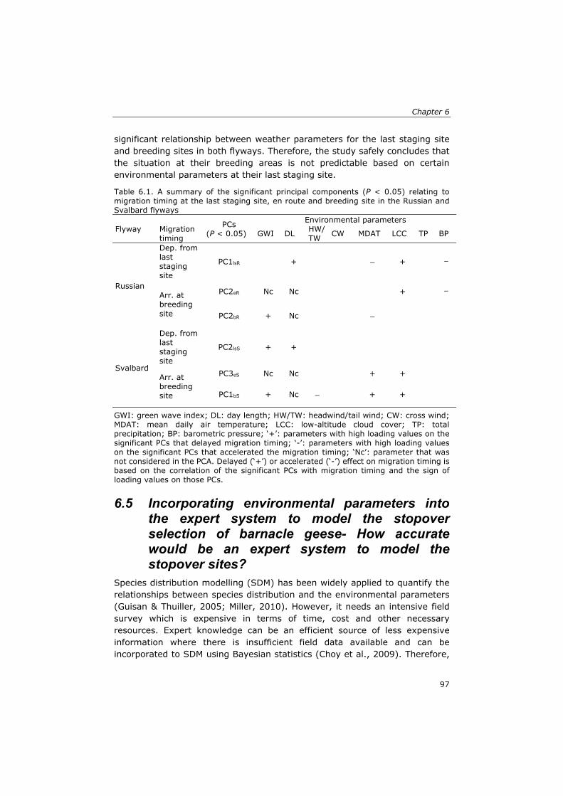
Chapter 6
97
significant relationship between weather parameters for the last staging site and breeding sites in both flyways. Therefore, the study safely concludes that the situation at their breeding areas is not predictable based on certain environmental parameters at their last staging site.
Table 6.1. A summary of the significant principal components (P < 0.05) relating to migration timing at the last staging site, en route and breeding site in the Russian and Svalbard flyways PCs
(P < 0.05)
Environmental parameters Flyway Migration
timing GWI DL HW/TW CW MDAT LCC TP BP
Russian
Dep. from last staging site
PC1lsR + +
Arr. at breeding site
PC2eR Nc Nc +
PC2bR + Nc
Svalbard
Dep. from last staging site
PC2lsS + +
Arr. at breeding site
PC3eS Nc Nc + +
PC1bS + Nc + +
GWI: green wave index; DL: day length; HW/TW: headwind/tail wind; CW: cross wind; MDAT: mean daily air temperature; LCC: low-altitude cloud cover; TP: total precipitation; BP: barometric pressure; ‘+’: parameters with high loading values on the significant PCs that delayed migration timing; ‘-’: parameters with high loading values on the significant PCs that accelerated the migration timing; ‘Nc’: parameter that was not considered in the PCA. Delayed (‘+’) or accelerated (‘-’) effect on migration timing is based on the correlation of the significant PCs with migration timing and the sign of loading values on those PCs.
6.5 Incorporating environmental parameters into the expert system to model the stopover selection of barnacle geese- How accurate would be an expert system to model the stopover sites?
Species distribution modelling (SDM) has been widely applied to quantify the relationships between species distribution and the environmental parameters (Guisan & Thuiller, 2005; Miller, 2010). However, it needs an intensive field survey which is expensive in terms of time, cost and other necessary resources. Expert knowledge can be an efficient source of less expensive information where there is insufficient field data available and can be incorporated to SDM using Bayesian statistics (Choy et al., 2009). Therefore,

Synthesis
98
we used Bayesian expert system to incorporate environmental parameters as data layers to model stopover selection of barnacle geese from Russian, Svalbard and Greenland populations. Environmental parameters have been grouped into four categories, i.e. human disturbance, site safety, roosting area and foraging habitat (Table 6.2).
Table 6.2. Environmental parameters (n=14) used to model the stopover selection of barnacle geese. Category Parameter
Human disturbance
Distance-to-cities (km) (>50,000 citizens) Distance-to-town (km) (<50,000 citizens) Distance-to-local road (km) Distance-to-major roads incl. highways (km) Distance-to-wind farms (km)
Site safety Distance-to-forest (km)
Roosting areas
Distance-to-inland water (km) Distance-to-ocean (km)
Distance-to-river (km)
Foraging habitat
Elevation (m)
Greenness factor (GWI) Percentage cover of grassland/ cropland Percentage cover of salt marsh Percentage cover of snow
Using Bayes’ theorem the posterior probability of presence and absence at each stopover site was calculated separately. Therefore, in the research results the Bayesian expert system would model the stopover selection correctly if the posterior probability of presence at stopover sites is higher than 0.5 (O'Hagan et al., 2006).
Incorporating all the parameters into the model, resulted in relatively low mean of posterior probabilities of presence at the stopover sites ( 0.5) for all three populations. However, for all three populations the highest posterior probability of presence ( 0.5) was observed when the salt marsh was removed from the Bayesian model. Furthermore, the posterior probability of presence at the stopover sites was significantly higher than posterior probability of absence (P<0.001, Mann-Whitney test).
The obtained results do not indicate that salt marshes have inferior importance for stopover selection by the geese, as they are among the important foraging habitat for barnacle geese (Prins & Ydenberg, 1985; van der Graaf et al., 2004). Based on the expert opinion, it is most likely that barnacle geese choose sites (salt marshes) with more than 50% coverage. However, in the current study, on average only 10% of the stopovers area were covered by this land cover. So it can be inferred that possibly the experts have underestimated the importance of small areas of salt marsh.

Chapter 6
99
6.6 Practical relevance Satellite-derived green wave index (GWI) provides the opportunity to study plant phenology in remote areas and assist to accurately predict the spring migration timing of Arctic-nesting geese with respect to the wave of high-nutrition plants.
The findings presented in Chapter 4 highlighted that the environmental parameters at the last staging site, which is both closer to, and the longest, stop before reaching the breeding site, in migration timing are very important. As it has been discussed by Bauer et al. (2008) the species or populations that are staging closer to their breeding site should be better able to adjust to climate change. Therefore, using GWI and the parameters (as identified in Chapter 4) might help to predict the consequences of future climate change on migration patterns. This is especially important for the high-Arctic breeders because spring advancement, which results from climate change, is more rapid there (IPCC, 2007; Stone et al., 2002). Moreover, integrating these parameters with energy cues could be used to build an optimal migration model so as to be able to predict migration timing of avian herbivores.
Besides the importance of understanding the effect of climate change on migration, it is essential to relieve the possible future conflicts of migratory geese with agriculture due to population expansion of the geese and their dependency on agricultural food (Cope et al., 2003). Therefore, to resolve this conflict the correct identification of stopover sites is necessary (Jensen et al., 2008). However, collecting data on species numbers and distributions from broad spatial extents using field-based methods can be prohibitively expensive. Nevertheless, remote sensing data provides an effective way to predict the distribution of species at different scales. Predicting and measuring the distribution of species using remote sensing data and geo-information technology would seem an ideal way to gather these crucial data. In fact, combining Bayesian expert system and remote sensing allows predicting the potential stopover sites of the geese on a large spatial scale.
6.7 Future Research Avenues Following recommendations are suggested to continue future works on this topic:
1) Building a prediction model for the geese arrival date at the breeding site using the significant environmental parameters at the last staging site that were identified in this thesis and the internal parameters.
2) Using a forward chaining expert system with non-informative prior to predict the potential stopover sites of the geese and validate the results with real data.

Synthesis
100
3) Examine the differences in respect to human disturbance and food quality and quantity between two different stopover sites in the Baltic region (i.e. Estonia and Gotland), and to investigate the change of environmental carrying capacity (by measuring biomass and human disturbance as a proxy of environmental carrying capacity) in whole Baltic region during two decades (i.e. 1990s and 2000s).

101
Bibliography AEWA. (2015). 6th Session of the meeting of the parties (Outcomes of the
international conference “Goose management: challenges 2015”). Bonn, Germany.
Åkesson, S., & Bäckman, J. (1999). Orientation in pied flycatchers: the relative importance of magnetic and visual information at dusk. Animal Behaviour, 57(4), 819-828.
Åkesson, S., Walinder, G., Karlsson, L., & Ehnbom, S. (2001). Reed warbler orientation: initiation of nocturnal migratory flights in relation to visibility of celestial cues at dusk. Animal Behaviour, 61(1), 181-189.
Alerstam, T. (2001). Evaluation of long-distance orientation in birds on the basis of migration routes recorded by radar and satellite tracking. The Journal of Navigation, 54(03), 393-403.
Alerstam, T., & Lindström, Å. (1990). Optimal bird migration: the relative importance of time, energy, and safety Bird migration (pp. 331-351): Springer.
Amano, T., Ushiyama, K., Fujita, G., & Higuchi, H. (2006). Foraging Patch Selection and Departure by Non-Omniscient Foragers: A Field Example in White-Fronted Geese. Ethology, 112(6), 544-553.
ARGOS/CLS. (2011). Argos user's manual. from http://www.grouptechnologies.com.au/downloads/apex/apex-argos-mk2-user-manual.pdf
Aspinall, R. (1992). An inductive modelling procedure based on Bayes' theorem for analysis of pattern in spatial data. International Journal of Geographical Information Systems, 6(2), 105-121.
Atzberger, C., Richter, K., Vuolo, F., Darvishzadeh, R., & Schlerf, M. (2011). Why confining to vegetation indices? Exploiting the potential of improved spectral observations using radiative transfer models. Paper presented at the SPIE Remote Sensing.
Bairlein, F. (2008). The mysteries of bird migration--Still much to be learnt. British Birds, 101(2), 68.
Ball, T. (1983). The migration of geese as an indicator of climate change in the southern Hudson Bay region between 1715 and 1851. Climatic Change, 5(1), 85-93.
Bartlam-Brooks, H. L. A., Beck, P. S. A., Bohrer, G., & Harris, S. (2013). In search of greener pastures: Using satellite images to predict the effects of environmental change on zebra migration. Journal of Geophysical Research: Biogeosciences, 118(4), 1427-1437.
Bates, D., Eigen, C., & Rcpp, L. (2014). Package ‘lme4’. Bauer, S., Gienapp, P., & Madsen, J. (2008). The relevance of environmental
conditions for departure decision changes en route in migrating geese. Ecology, 89(7), 1953-1960.

Bibliography
102
Bauer, S., Madsen, J., & Klaassen, M. (2006). Intake rates, stochasticity, or onset of spring: what aspects of food availability affect spring migration patterns in Pink-footed Geese Anser brachyrhynchus? Ardea, 94(3), 555-566.
Bauer, S., Nolet, B. N., Giske, J., Chapman, J. W., Åkesson, S., Hedenström, A., & Fryxel, J. M. (2011). Cues and decision rules in animal migration. In E. J. Milner-Gulland, J. M. Fryxell, & A. R. E. Sinclair (Eds.), Animal Migration-A Synthesis (pp. 68-87): Oxford University Press.
Beck, P. S. A., Atzberger, C., Høgda, K. A., Johansen, B., & Skidmore, A. K. (2006). Improved monitoring of vegetation dynamics at very high latitudes: A new method using MODIS NDVI. Remote Sensing of Environment, 100(3), 321-334.
Beck, P. S. A., Jönsson, P., Høgda, K. A., Karlsen, S. R., Eklundh, L., & Skidmore, A. K. (2007). A ground‐validated NDVI dataset for monitoring vegetation dynamics and mapping phenology in Fennoscandia and the Kola peninsula. International Journal of Remote Sensing, 28(19), 4311-4330.
Beck, P. S. A., Wang, T. J., Skidmore, A. K., & Liu, X. H. (2008). Displaying remotely sensed vegetation dynamics along natural gradients for ecological studies. International Journal of Remote Sensing, 29(14), 4277-4283.
Beest, F. M., Uzal, A., Vander Wal, E., Laforge, M. P., Contasti, A. L., Colville, D., & McLoughlin, P. D. (2014). Increasing density leads to generalization in both coarse‐grained habitat selection and fine‐grained resource selection in a large mammal. Journal of Animal Ecology, 83(1), 147-156.
Berberan-Santos, M. N., Bodunov, E. N., & Pogliani, L. (1997). On the barometric formula. American Journal of Physics, 65(5), 404-412.
Bergman, G. (1978). Effects of wind conditions on the autumn migration of waterfowl between the White Sea area and the Baltic region. Oikos, 393-397.
Berthold, P. (1999). A comprehensive theory for the evolution, control and adaptability of avian migration. Ostrich, 70(1), 1-11.
Berthold, P., Bauer, H.-G., & Westhead, V. (2001). Bird migration: a general survey (Vol. 12): Oxford University Press Oxford.
Berthold, P., Gwinner, E., & Sonnenschein, E. (Eds.). (2003). Avian migration. Verlag Berlin Heidelberg: Springer.
Bety, J., Giroux, J. F., & Gauthier, G. (2004). Individual variation in timing of migration: causes and reproductive consequences in greater snow geese (Anser caerulescens atlanticus). Behavioral Ecology and Sociobiology, 57(1), 1-8.
Bischof, R., Loe, L.E., Meisingset, E.L., Zimmermann, B., Van Moorter, B., & Mysterud, A. (2012). A Migratory Northern Ungulate in the Pursuit of Spring: Jumping or Surfing the Green Wave? American Naturalist, 180(4), 407-424.

Bibliography
103
Black, J. M., Prop, J., & Larsson, K. (2007). Wild goose dilemmas. Groningen, The Netherlands: Branta Press.
Bland, J. M., & Altman, D. G. (1995). Comparing methods of measurement: why plotting difference against standard method is misleading. The Lancet, 346(8982), 1085-1087.
Bliss, L. (1962). Adaptations of arctic and alpine plants to environmental conditions. Arctic, 15, 117-144.
Bliss, L. C. (1971). Arctic and Alpine Plant Life Cycles. Annual Review of Ecology and Systematics, 2(ArticleType: research-article / Full publication date: 1971 / Copyright © 1971 Annual Reviews), 405-438.
Bohrer, G., Beck, P. S., Ngene, S. M., Skidmore, A. K., & Douglas-Hamilton, I. (2014). Elephant movement closely tracks precipitation-driven vegetation dynamics in a Kenyan forest-savanna landscape. Movement Ecology, 2(1), 2.
Bolker, B. M., Brooks, M. E., Clark, C. J., Geange, S. W., Poulsen, J. R., Stevens, M. H. H., & White, J.-S. S. (2009). Generalized linear mixed models: a practical guide for ecology and evolution. Trends in Ecology and Evolution, 24(3), 127-135.
Botta, A., Viovy, N., Ciais, P., Friedlingstein, P., & Monfray, P. (2000). A global prognostic scheme of leaf onset using satellite data. Global Change Biology, 6(7), 709-725.
Box, E., Holben, B., & Kalb, V. (1989). Accuracy of the AVHRR vegetation index as a predictor of biomass, primary productivity and net CO2 flux. Vegetatio, 80(2), 71-89.
Bridge, E.S., Thorup, K., Bowlin, M.S., Chilson, P.B., Diehl, R.H., Fléron, R.W., Robinson, W. D. (2011). Technology on the move: recent and forthcoming innovations for tracking migratory birds. Bioscience, 61(9), 689-698.
Brotons, L., Thuiller, W., Araújo, M.B., & Hirzel, A.H. (2004). Presence‐absence versus presence‐only modelling methods for predicting bird habitat suitability. Ecography, 27(4), 437-448.
Brown, C.R., & Brown, M.B. (2000). Weather-mediated natural selection on arrival time in cliff swallows (Petrochelidon pyrrhonota). Behavioral Ecology and Sociobiology, 47(5), 339-345.
Burgan, R.E. (1996). Use of remotely sensed data for fire danger estimation. Earsel advances in remote sensing, 4(4), 1-8.
Butler, P.J., Woakes, A.J., & Bishop, C.M. (1998). Behaviour and physiology of Svalbard Barnacle Geese Branta leucopsis during their autumn migration. Journal of Avian Biology, 29(4), 536-545.
Chapin III, F. (1983). Direct and indirect effects of temperature on arctic plants. Polar Biology, 2(1), 47-52.
Chen, J., Jonsson, P., Tamura, M., Gu, Z.H., Matsushita, B., & Eklundh, L. (2004). A simple method for reconstructing a high-quality NDVI time-series data set based on the Savitzky-Golay filter. Remote Sensing of Environment, 91(3-4), 332-344.

Bibliography
104
Chmielewski, F.M., & Rotzer, T. (2001). Response of tree phenology to climate change across Europe. Agricultural and Forest Meteorology, 108(2), 101-112.
Choy, S.L., O'Leary, R., & Mengersen, K. (2009). Elicitation by design in ecology: using expert opinion to inform priors for Bayesian statistical models. Ecology, 90(1), 265-277.
Chudzińska, M.E., van Beest, F.M., Madsen, J., & Nabe-Nielsen, J. (2015). Using habitat selection theories to predict the spatiotemporal distribution of migratory birds during stopover – a case study of pink-footed geese Anser brachyrhynchus. Oikos, 124(7), 851-860.
Churkina, G., & Running, S.W. (1998). Contrasting Climatic Controls on the Estimated Productivity of Global Terrestrial Biomes. Ecosystems, 1(2), 206-215.
Cleland, E.E., Chuine, I., Menzel, A., Mooney, H.A., & Schwartz, M.D. (2007). Shifting plant phenology in response to global change. Trends in Ecology and Evolution, 22(7), 357-365.
Cope, D.R., Pettifor, R.A., Griffin, L.R., & Rowcliffe, J.M. (2003). Integrating farming and wildlife conservation: the Barnacle Goose Management Scheme. Biological Conservation, 110(1), 113-122.
Črepinšek, Z., Kajfež-Bogataj, L., & Bergant, K. (2006). Modelling of weather variability effect on fitophenology. Ecological Modelling, 194(1–3), 256-265.
De la Cueva, H., & Blake, R. (1993). Mechanics and energetics of ground effect in flapping flight. Contemp Math, 141, 421-442.
De Lucia, F.C., & Gottfried, J. L. (2011). Influence of variable selection on partial least squares discriminant analysis models for explosive residue classification. Spectrochimica Acta Part B: Atomic Spectroscopy, 66(2), 122-128.
Demment, M.W., & Van Soest, P.J. (1985). A nutritional explanation for body-size patterns of ruminant and nonruminant herbivores. The American Naturalist, 125(4), 641-672.
Di Marco, M., Buchanan, G.M., Szantoi, Z., Holmgren, M., Marasini, G.G., Gross, D., Rondinini, C. (2014). Drivers of extinction risk in African mammals: the interplay of distribution state, human pressure, conservation response and species biology. Philosophical Transactions of the Royal Society B: Biological Sciences, 369(1643), 20130198.
Dierschke, V., & Delingat, J. (2001). Stopover behaviour and departure decision of northern wheatears, Oenanthe oenanthe, facing different onward non-stop flight distances. Behavioral Ecology and Sociobiology, 50(6), 535-545.
Dobson, A.J., & Barnett, A. (2008). An introduction to generalized linear models: CRC press.
Dodge, S., Bohrer, G., Weinzierl, R., Davidson, S.C., Kays, R., Douglas, D., Wikelski, M. (2013). The environmental-data automated track annotation

Bibliography
105
(Env-DATA) system: linking animal tracks with environmental data. Movement Ecology, 1(1), 3.
Doiron, M., Legagneux, P., Gauthier, G., & Levesque, E. (2013). Broad-scale satellite Normalized Difference Vegetation Index data predict plant biomass and peak date of nitrogen concentration in Arctic tundra vegetation. Applied Vegetation Science, 16(2), 343-351.
Drent, R., Eichhorn, G., Flagstad, A., Van der Graaf, A., Litvin, K., & Stahl, J. (2007). Migratory connectivity in Arctic geese: spring stopovers are the weak links in meeting targets for breeding. Journal of Ornithology, 148(0), 501-514.
Drewitt, A. L., & Langston, R. H. (2006). Assessing the impacts of wind farms on birds. Ibis, 148(s1), 29-42.
Duncan, C., Abel, B., Kwan, D., & Mehlman, D. (2002). The Nature Conservancy's Gulf Wings Project – A Case Study in Conservation Planning for Migratory Birds. Paper presented at the Third International Partners in Flight Conference, Asilomar Conference Grounds, California.
Duriez, O., Bauer, S., Destin, A., Madsen, J., Nolet, B.A., Stillman, R.A., & Klaassen, M. (2009). What decision rules might pink-footed geese use to depart on migration? An individual-based model. Behavioral Ecology, 20(3), 560-569.
Eichhorn, G., Afanasyev, V., Drent, R.H., & van der Jeugd, H.P. (2006). Spring stopover routines in Russian Barnacle Geese Branta leucopsis tracked by resightings and geolocation. Ardea, 94(3), 667-678.
Eichhorn, G., Drent, R.H., Stahl, J., Leito, A., & Alerstam, T. (2009). Skipping the Baltic: the emergence of a dichotomy of alternative spring migration strategies in Russian barnacle geese. Journal of Animal Ecology, 78(1), 63-72.
Elith, J., Graham, C., Anderson, R., Dudík, M., Ferrier, S., Guisan, A., G Lohmann, L. (2006). Novel methods improve prediction of species’ distributions from occurrence data. Ecography, 29(2), 129-151.
Ellison, A.M. (1996). An Introduction to Bayesian Inference for Ecological Research and Environmental Decision-Making. Ecological Applications, 6(4), 1036-1046.
Ellison, A.M. (2004). Bayesian inference in ecology. Ecology Letters, 7(6), 509-520.
Ens, B.J., Bairlein, F., Camphuysen, C.J., de Boer, R., Exo, K.M., Gallego, N., Van Gasteren, H. (2008). Tracking of individual birds. Report on WP 3230 (bird tracking sensor characterization) and WP 4130 (sensor adaptation and calibration for bird tracking system) of the FlySafe basic activities project: SOVON-onderzoeksrapport 2008/10.SOVON Vogelonderzoek Nederland, Beek-Ubbergen, the Netherlands.
EPA. (2000). Meteorological Monitoring Guidance for Regulatory Modeling Applications. United States: Environmental protection agency.

Bibliography
106
Erni, B., Liechti, F., & Bruderer, B. (2005). The role of wind in passerine autumn migration between Europe and Africa. Behavioral Ecology, 16(4), 732-740.
ESRI. (2016). Arc GIS online. from http://www.arcgis.com/home/index.html Faaborg, J., Holmes, R. T., Anders, A. D., Bildstein, K. L., Dugger, K. M.,
Gauthreaux, S.A., Warnock, N. (2010). Conserving migratory land birds in the New World: Do we know enough? Ecological Applications, 20(2), 398-418.
Fiedler, W. (2009). New technologies for monitoring bird migration and behaviour. Ringing & Migration, 24(3), 175-179.
Finn, J., Carlsson, J., Kelly, T., & Davenport, J. (2012). Avoidance of headwinds or exploitation of ground effect—why do birds fly low? Journal of Field Ornithology, 83(2), 192-202.
Fitzjarrald, D. R., Acevedo, O. C., & Moore, K. E. (2001). Climatic consequences of leaf presence in the eastern United States. Journal of Climate, 14(4), 598-614.
Fox, A., Francis, I. S., & Bergersen, E. (2006). Diet and habitat use of Svalbard Pink-footed Geese Anser brachyrhynchus during arrival and pre-breeding periods in Adventdalen. Ardea, 94(3), 691.
Fryxell, J.M. (1991). Forage quality and aggregation by large herbivores. American Naturalist, 138(2), 478-498.
Fujioka, E., Soldevilla, M.S., Read, A. J., & Halpin, P. N. (2013). Integration of passive acoustic monitoring data into OBIS-SEAMAP, a global biogeographic database, to advance spatially-explicit ecological assessments. Ecological Informatics, 21, 59-73.
Ganter, B., Larsson, K., Syroechkovsky, E. V., Litvin, K. E., Leito, A., & Madsen, J. (1999). Barnacle Geese Branta leucopsis: Russia/Baltic. In J. Madsen, G. Cracknell, & T. Fox (Eds.), Goose populations of the western palearctic: A review of status and distribution. Rond, Denmark: National Environmental Research Institute.
Gauthier, G., Bêty, J., Cadieux, M.-C., Legagneux, P., Doiron, M., Chevallier, C., Berteaux, D. (2013). Long-term monitoring at multiple trophic levels suggests heterogeneity in responses to climate change in the Canadian Arctic tundra. Philosophical Transactions of the Royal Society of London B: Biological Sciences, 368(1624), 20120482.
Gauthier, G., Bety, J., & Hobson, K.A. (2003). Are greater snow geese capital breeders? New evidence from a stable-isotope model. Ecology, 84(12), 3250-3264.
Gill, J.A. (1996). Habitat choice in pink-footed geese: quantifying the constraints determining winter site use. Journal of Applied Ecology, 884-892.
Gillespie, T.W. (2001). Remote sensing of animals. Progress in Physical Geography, 25(3), 355-362.

Bibliography
107
Godvik, I.M.R., Loe, L.E., Vik, J.O., Veiberg, V., Langvatn, R., & Mysterud, A. (2009). Temporal scales, trade-offs, and functional responses in red deer habitat selection. Ecology, 90(3), 699-710.
Gordo, O. (2007). Why are bird migration dates shifting? A review of weather and climate effects on avian migratory phenology. Climate Research, 35(1-2), 37-58.
Gordo, O., & Sanz, J.J. (2009). Long-term temporal changes of plant phenology in the Western Mediterranean. Global Change Biology, 15(8), 1930-1948.
Gordo, O., & Sanz, J.J. (2010). Impact of climate change on plant phenology in Mediterranean ecosystems. Global Change Biology, 16(3), 1082-1106.
Green, M., Alerstam, T., Clausen, P., Drent, R., & Ebbinge, B.S. (2002). Dark‐bellied Brent Geese Branta bernicla bernicla, as recorded by satellite telemetry, do not minimize flight distance during spring migration. Ibis, 144(1), 106-121.
Griffin, L.R. (2008). Identifying the pre-breeding areas of the Svalbard Barnacle Goose Branta leucopsis between mainland Norway and Svalbard: an application of GPS satellite-tracking techniques. Vogelwelt, 129, 226-232.
Guan, H., & Hiroyoshi, H. (1999). Review on satellite tracking of migratory birds and its prospect. Zoological research/" Dong wu xue yan jiu" bian ji wei yuan hui bian ji, 21(5), 412-415.
Guisan, A., & Thuiller, W. (2005). Predicting species distribution: offering more than simple habitat models. Ecology Letters, 8(9), 993-1009.
Guisan, A., & Zimmermann, N. E. (2000). Predictive habitat distribution models in ecology. Ecological Modelling, 135(2–3), 147-186.
Gullestad, N., Owen, M., & Nugent, M. (1984). Numbers and distribution of Barnacle Geese Branta leucopsis on Norwegian staging islands and the importance of the staging area to the Svalbard population. Norsk Polarinstitutt Skrifter, 181, 57-65.
Guo-Gang, Z., Dong-Ping, L., Yun-Qiu, H., Hong-Xing, J., Ming, D., Fa-Wen, Q., Feng-Shan, L. (2011). Migration routes and stop-over sites determined with satellite tracking of bar-headed geese Anser indicus breeding at Qinghai Lake, China. Waterbirds, 34(1), 112-116.
Gwinner, E. (2012). Bird migration: physiology and ecophysiology: Springer Science & Business Media.
Hahn, S., Loonen, M. J., & Klaassen, M. (2011). The reliance on distant resources for egg formation in high Arctic breeding barnacle geese Branta leucopsis. Journal of Avian Biology, 42(2), 159-168.
Hamel, S., Garel, M., Festa-Bianchet, M., Gaillard, J. M., & Cote, S. D. (2009). Spring Normalized Difference Vegetation Index (NDVI) predicts annual variation in timing of peak faecal crude protein in mountain ungulates. Journal of Applied Ecology, 46(3), 582-589.

Bibliography
108
Hedenström, A., & Alerstam, T. (1997). Optimum fuel loads in migratory birds: distinguishing between time and energy minimization. Journal of Theoretical Biology, 189(3), 227-234.
Hord, C. (2011). Report of the ad-hoc working group on the calculation of crosswind and tailwind components with particular regard to the inclusion of gusts. Paper presented at the Aerodrome Meteorological Observation and Forecast Study Group (AMOFSG), Montréal.
Hübner, C.E. (2006). The importance of pre-breeding areas for the Arctic Barnacle Goose Branta leucopsis. Ardea, 94(3), 701-713.
Hübner, C.E., Tombre, I.M., Griffin, L.R., Loonen, M., Shimmings, P., & Jonsdottir, I. S. (2010). The connectivity of spring stopover sites for geese heading to arctic breeding grounds. Ardea, 98(2), 145-154.
Huete, A., Didan, K., Miura, T., Rodriguez, E.P., Gao, X., & Ferreira, L.G. (2002). Overview of the radiometric and biophysical performance of the MODIS vegetation indices. Remote Sensing of Environment, 83(1-2), 195-213.
Hume, R. (1986). Reactions of birds to heavy rain. British Birds, 79, 326-329. Hupp, J. W., Zacheis, A. B., Anthony, R. M., Robertson, D. G., Erickson, W. P.,
& Palacios, K. C. (2001). Snow cover and snow goose Anser caerulescens caerulescens distribution during spring migration. Wildlife Biology, 7(2), 65-76.
Hurlbert, S.H. (1984). Pseudoreplication and the Design of Ecological Field Experiments. Ecological Monographs, 54(2), 187-211.
Hustings, F. (1992). European Monitoring Studies on Breeding Birds: An Update. Bird Census News, 5(2), 1-56.
IPCC. (2007). Climate Change 2007: Synthesis Report. Contribution of Working Groups I, II and III to 534 the Fourth Assessment Report of the Intergovernmental Panel on Climate Change. Geneva, Switzerland.
Ito, T.Y., Miura, N., Lhagvasuren, B., Enkhbileg, D., Takatsuki, S., Tsunekawa, A., & Jiang, Z. (2006). Satellite tracking of Mongolian gazelles (Procapra gutturosa) and habitat shifts in their seasonal ranges. Journal of Zoology, 269(3), 291-298.
James, A., Gaston, K.J., & Balmford, A. (2001). Can We Afford to Conserve Biodiversity? Bioscience, 51(1), 43-52.
Jankowiak, L., Antczak, M., & Tryjanowski, P. (2008). Habitat use, food and the importance of poultry in the diet of the red fox Vulpes vulpes in extensive farmland in Poland. World Appl Sci J, 4, 886-890.
Jenni, L., & Schaub, M. (2003). Behavioural and physiological reactions to environmental variation in bird migration: a review Avian migration (pp. 155-171): Springer.
Jensen, G.H., Madsen, J., Johnson, F.A., & Tamstorf, M.P. (2014). Snow conditions as an estimator of the breeding output in high-Arctic pink-footed geese Anser brachyrhynchus. Polar Biology, 37(1), 1-14.

Bibliography
109
Jensen, R.A., Wisz, M.S., & Madsen, J. (2008). Prioritizing refuge sites for migratory geese to alleviate conflicts with agriculture. Biological Conservation, 141(7), 1806-1818.
Jia, G.S.J., Epstein, H.E., & Walker, D.A. (2003). Greening of arctic Alaska, 1981-2001. Geophysical Research Letters, 30(20), 1-4.
Jonker, R.M., Eichhorn, G., Van Langevelde, F., & Bauer, S. (2010). Predation danger can explain changes in timing of migration: the case of the barnacle goose. Plos One, 5(6), e11369-e11369.
Jonsson, A.M., Eklundh, L., Hellstrom, M., Barring, L., & Jonsson, P. (2010). Annual changes in MODIS vegetation indices of Swedish coniferous forests in relation to snow dynamics and tree phenology. Remote Sensing of Environment, 114(11), 2719-2730.
Justice, C.O., Townshend, J.R.G., Holben, B.N., & Tucker, C.J. (1985). Analysis of the phenology of global vegetation using meteorological satellite data. International Journal of Remote Sensing, 6(8), 1271-1318.
Kaiser, D.P. (2000). Decreasing cloudiness over China: An updated analysis examining additional variables. Geophysical Research Letters, 27(15), 2193-2196.
Keller, V. (1991). The effect of disturbance from roads on the distribution of feeding sites of geese (Anser-brachyrhynchus, A. anser), wintering in north-east Scotland. Ardea, 79(2), 228-231.
Kerby, J., & Post, E. (2013). Reproductive Phenology of Large Mammals Phenology: An Integrative Environmental Science (pp. 467-479): Springer.
Kerlinger, P., & Moore, F.R. (1989). Atmospheric structure and avian migration Current ornithology (pp. 109-142): Springer.
Kerr, J.T., & Ostrovsky, M. (2003). From space to species: ecological applications for remote sensing. Trends in Ecology and Evolution, 18(6), 299-305.
Kirk, J. (1994). Light and photosynthesis in aquatic ecosystems: Cambridge University Press, London.
Klaassen, R.H., Hake, M., Strandberg, R., Koks, B.J., Trierweiler, C., Exo, K.M., Alerstam, T. (2014). When and where does mortality occur in migratory birds? Direct evidence from long‐term satellite tracking of raptors. Journal of Animal Ecology, 83(1), 176-184.
Kokko, H. (1999). Competition for early arrival in migratory birds. Journal of Animal Ecology, 68(5), 940-950.
Kölzsch, A., Bauer, S., Boer, R. d., Griffin, L., Cabot, D., Exo, K., Nolet, B.A. (2015). Forecasting spring from afar? Timing of migration and predictability of phenology along different migration routes of an avian herbivore. Journal of Animal Ecology, 84, 272-283.
Kölzsch, A., Müskens, G., Kruckenberg, H., Glazov, P., Weinzierl, R., Nolet, B., & Wikelski, M. (2016). Towards a new understanding of migration timing: slower spring than autumn migration in geese reflects different decision

Bibliography
110
rules for stopover use and departure. Oikos, Vol. in press. ISSN 1600-0706.
Kostin, I.O., & Mooij, J.H. (1995). Influence of weather conditions and other factors on the reproductive cycle of red-breasted geese Branta ruficollis on the Taymyr Peninsula. Wildfowl, 46(46), 45-54.
Krebs, C.J. (2001). Ecology: the experimental analysis of distribution and abundance. San Francisco: Benjamin Cummings.
Kruckenberg, H., & Jaene, J. (1999). Zum Einfluss eines Windparks auf die Verteilung weidender Bläßgänse im Rheiderland (Landkreis Leer, Niedersachsen). Natur und Landschaft, 74(10), 420-427.
Kuznetsova, A., Brockhoff, P.B., & Christensen, R.H.B. (2014). Package ‘lmerTest’.
Kynn, M. (2005). Eliciting expert knowledge for Bayesian logistic regression in species habitat modelling. (PhD), Qeensland University of Technology.
Langston, R., & Pullan, J. (2003). Wind farms and birds: an analysis of the effects of wind farms on birds, and guidance on environmental assessment criteria and site selection issues: BirdLife International to the Council of Europe, Bern Convention on the Conservation of European Wildlife and Natural Habitats. RSPB/BirdLife in the UK.
Langston, R.H. (2013). Birds and wind projects across the pond: A UK perspective. Wildlife Society Bulletin, 37(1), 5-18.
Lantinga, E.A. (1985). Productivity of grasslands under continuous and rotational grazing. (PhD thesis), University of Wageningen, The Netherlands.
Larsen, J.K., & Madsen, J. (2000). Effects of wind turbines and other physical elements on field utilization by pink-footed geese (Anser brachyrhynchus): A landscape perspective. Landscape ecology, 15(8), 755-764.
Lee, K.N. (1994). Compass and gyroscope: integrating science and politics for the environment: Island Press.
Lendrum, P.E., Anderson, C.R., Monteith, K.L., Jenks, J.A., & Bowyer, R.T. (2014). Relating the movement of a rapidly migrating ungulate to spatiotemporal patterns of forage quality. Mammalian Biology-Zeitschrift für Säugetierkunde, 79(6), 369-375.
Lessells, C., & Boag, P. T. (1987). Unrepeatable repeatabilities: a common mistake. The Auk, 104, 116-121.
Liechti, F. (2006). Birds: blowin’by the wind? Journal of Ornithology, 147(2), 202-211.
Liston, G.E., & Sturm, M. (2002). Winter precipitation patterns in arctic Alaska determined from a blowing-snow model and snow-depth observations. Journal of Hydrometeorology, 3(6), 646-659.
Loe, L., Bonenfant, C., Mysterud, A., GAILLARD, J.M., Langvatn, R., Klein, F., Stenseth, N. (2005). Climate predictability and breeding phenology in red

Bibliography
111
deer: timing and synchrony of rutting and calving in Norway and France. Journal of Animal Ecology, 74(4), 579-588.
Lofts, B., & Murton, R.K. (1968). Photoperiodic and physiological adaptations regulating avian breeding cycles and their ecological significance. Journal of Zoology, 155(3), 327-394.
Lorentsen, S.H., Oien, I.J., & Aarvak, T. (1998). Migration of Fennoscandian lesser white-fronted geese Anser erythropus mapped by satellite telemetry. Biological Conservation, 84(1), 47-52.
Lourenço, P.M., Kentie, R., Schroeder, J., Groen, N.M., Hooijmeijer, J.C., & Piersma, T. (2011). Repeatable timing of northward departure, arrival and breeding in Black-tailed Godwits Limosa l. limosa, but no domino effects. Journal of Ornithology, 152(4), 1023-1032.
Ma, Z., Hua, N., Zhang, X., Guo, H., Zhao, B., Ma, Q., Tang, C. (2011). Wind conditions affect stopover decisions and fuel stores of shorebirds migrating through the south Yellow Sea. Ibis, 153(4), 755-767.
Madritch, M.D., Kingdon, C.C., Singh, A., Mock, K.E., Lindroth, R.L., & Townsend, P.A. (2014). Imaging spectroscopy links aspen genotype with below-ground processes at landscape scales. Philosophical Transactions of the Royal Society B: Biological Sciences, 369(1643), 20130194.
Madsen, J. (1985). Impact of disturbance on field utilization of pink-footed geese in West Jutland, Denmark. Biological Conservation, 33(1), 53-63.
Madsen, J. (2001). Spring migration strategies in Pink-footed Geese Anser brachyrhynchus and consequences for spring fattening and fecundity. Ardea, 89(1), 43-55.
Madsen, J., Bjerrum, M., & Tombre, I.M. (2014). Regional management of farmland feeding geese using an ecological prioritization tool. Ambio, 43(6), 801-809.
Madsen, J., Cracknell, G., & Fox, T. (1999). Goose populations of the Western Palearctic: a review of status and distribution: National Environmental Research Institute Rønde.
Madsen, J., Tamstorf, M., Klaassen, M., Eide, N., Glahder, C., Riget, F., Cottaar, F. (2007). Effects of snow cover on the timing and success of reproduction in high-Arctic pink-footed geese Anser brachyrhynchus. Polar Biology, 30(11), 1363-1372.
Marshal, J.P., Bleich, V.C., Krausman, P.R., Reed, M.L., & Andrew, N.G. (2006). Factors affecting habitat use and distribution of desert mule deer in an arid environment. Wildlife Society Bulletin, 34(3), 609-619.
Maselli, F., Petkov, L., & Maracchi, G. (1998). Extension of climate parameters over the land surface by the use of NOAA-AVHRR and ancillary data. Photogrammetric Engineering and Remote Sensing, 64(3), 199-206.
Mathworks. (2013). Matlab, The language of technical computing. Mathworks, INC. USA.
McCarthy, M.A. (2007). Bayesian methods for ecology: Cambridge University Press.

Bibliography
112
McGarigal, K., Cushman, S., & Stafford, S. (2000). Multivariate statistics for wildlife and ecology research. New York: Springer.
McMaster, G.S., & Wilhelm, W.W. (1997). Growing degree-days: one equation, two interpretations. Agricultural and Forest Meteorology, 87(4), 291-300.
McNamara, J. M., Barta, Z., Klaassen, M., & Bauer, S. (2011). Cues and the optimal timing of activities under environmental changes. Ecology Letters, 14(12), 1183-1190.
Mehlman, D.W., Mabey, S.E., Ewert, D.N., Duncan, C., Abel, B., Cimprich, D., Woodrey, M. (2005). Conserving stopover sites for forest-dwelling migratory landbirds. The Auk, 122(4), 1281-1290.
Meijer, T., & Drent, R. (1999). Re‐examination of the capital and income dichotomy in breeding birds. Ibis, 141(3), 399-414.
Menzel, A., Sparks, T.H., Estrella, N., Koch, E., Aasa, A., Ahas, R., Zust, A. (2006). European phenological response to climate change matches the warming pattern. Global Change Biology, 12(10), 1969-1976.
Microwave Telemetry. (2007). Argos/GPS PTT-100 Field Manual. Microwave Telemetry, Inc.
Miller, J. (2010). Species distribution modeling. Geography Compass, 4(6), 490-509.
Mueller, T., Olson, K.A., Fuller, T.K., Schaller, G.B., Murray, M.G., & Leimgruber, P. (2008). In search of forage: predicting dynamic habitats of Mongolian gazelles using satellite-based estimates of vegetation productivity. Journal of Applied Ecology, 45(2), 649-658.
Muñoz, A.-R., Márquez, A L., & Real, R. (2015). An approach to consider behavioral plasticity as a source of uncertainty when forecasting species' response to climate change. Ecology and Evolution, 1-15.
Murphy-Klassen, H.M., Underwood, T.J., Sealy, S.G., Czyrnyj, A.A., & Holberton, R. (2005). Long-term trends in spring arrival dates of migrant birds at Delta Marsh, Manitoba, in relation to climate change. The Auk, 122(4), 1130-1148.
Murray, J.V., Goldizen, A.W., O’Leary, R.A., McAlpine, C.A., Possingham, H.P., & Choy, S.L. (2009). How useful is expert opinion for predicting the distribution of a species within and beyond the region of expertise? A case study using brush‐tailed rock‐wallabies Petrogale penicillata. Journal of Applied Ecology, 46(4), 842-851.
Myneni, R.B., Hall, F.G., Sellers, P.J., & Marshak, A.L. (1995). The interpretation of spectral vegetation indexes. IEEE Transactions on Geoscience and Remote Sensing, 33(2), 481-486.
Myneni, R.B., Keeling, C., Tucker, C., Asrar, G., & Nemani, R. (1997). Increased plant growth in the northern high latitudes from 1981 to 1991. Nature, 386(6626), 698-702.
Nakagawa, S., & Schielzeth, H. (2010). Repeatability for Gaussian and non‐Gaussian data: a practical guide for biologists. Biological Reviews, 85(4), 935-956.

Bibliography
113
Naylor, C. (1989). How to build an inferencing engine Expert systems principles and case studies (pp. 84): Chapman \& Hall, Ltd.
Nemani, R.R., Keeling, C.D., Hashimoto, H., Jolly, W.M., Piper, S.C., Tucker, C. J., Running, S. W. (2003). Climate-driven increases in global terrestrial net primary production from 1982 to 1999. Science, 300(5625), 1560-1563.
Newton, L. (2008). The Migration Ecology of Birds: Academic Press is an imprint of Elsevier.
Niamir, A., Skidmore, A.K., Toxopeus, A.G., Muñoz, A.-R., & Real, R. (2011). Finessing atlas data for species distribution models. Diversity and Distributions, 17(6), 1173-1185.
Nielsen, A., Steinheim, G., & Mysterud, A. (2013). Do different sheep breeds show equal responses to climate fluctuations? Basic and Applied Ecology, 14(2), 137-145.
Niles, L.J., Burger, J., & Kathleen, E.C. (1996). The influence of weather, geography, and habitat on migrating raptors on Cape May PenInsuila. The Condor, 93, 382-394.
Nilsson, A.L.K., Alerstam, T., & Nilsson, J.-Å. (2006). DO PARTIAL AND REGULAR MIGRANTS DIFFER IN THEIR RESPONSES TO WEATHER? The Auk, 123(2), 537-547.
Norris, D.R., Marra, P.P., Kyser, T.K., Sherry, T.W., & Ratcliffe, L.M. (2004). Tropical winter habitat limits reproductive success on the temperate breeding grounds in a migratory bird. Proceedings of the Royal Society of London B: Biological Sciences, 271(1534), 59-64.
O'Hagan, A., Buck, C.E., Daneshkhah, A., Eiser, J.R., Garthwaite, P.H., Jenkinson, D.J., Rakow, T. (2006). Uncertain judgements: eliciting experts' probabilities: John Wiley & Sons.
Ogilvie, M.A., Boertmann, D., Cabot, D., Merne, O., Percival, S.M., & Sigfusson, A. (1999). Barnacle Goose Branta leucopsis: Greenland. In J. Madsen, G. Cracknell, & T. Fox (Eds.), Goose Populations of the Western Palearctic. A Review of Status and Distribution. (pp. 344 ). Rond, Denmark: National Environmental Research Institute.
Olivier, F., & Wotherspoon, S.J. (2005). GIS-based application of resource selection functions to the prediction of snow petrel distribution and abundance in East Antarctica: Comparing models at multiple scales. Ecological Modelling, 189(1-2), 105-129.
Owen, M. (1980). Wild Geese of the World. London, UK: B. T. Batsford Ltd. Pearce-Higgins, J., Yalden, D., & Whittingham, M. (2005). Warmer springs
advance the breeding phenology of golden plovers Pluvialis apricaria and their prey (Tipulidae). Oecologia, 143(3), 470-476.
Pedersen, M., & Poulsen, E. (1991). Impact of a 90m/2MW wind turbine on birds: Avian response to the implementation of the Tjaereborg Wind Turbine at the Danish Wadden Sea. Danske Vildtundersoegelser (Denmark).

Bibliography
114
Pedrana, J., Pon, J P.S., Isacch, J. P., Leiss, A., Rojas, P.O., Castresana, G., Maceira, N. O. (2015). First insights into the migration pattern of an upland goose (Chloephaga picta) based on satellite tracking. Ornitología Neotropical, 26, 245-253.
Pendlebury, C., Zisman, S., Walls, R., Sweeney, J., McLoughlin, E., Robinson, C., Loughrey, J. (2011). Literature review to assess bird specis connectivity to Special Protection Areas: Scottish Natural Heritage Commissioned Report No. 390, UK.
Pettorelli, N., Ryan, S., Mueller, T., Bunnefeld, N., Jędrzejewska, B., Lima, M., & Kausrud, K. (2011). The Normalized Difference Vegetation Index (NDVI): unforeseen successes in animal ecology. Climate Research, 46(1), 15-27.
Pettorelli, N., Vik, J. O., Mysterud, A., Gaillard, J.-M., Tucker, C.J., & Stenseth, N.C. (2005). Using the satellite-derived NDVI to assess ecological responses to environmental change. Trends in Ecology and Evolution, 20(9), 503-510.
Phillips, S.J., Anderson, R.P., & Schapire, R.E. (2006). Maximum entropy modeling of species geographic distributions. Ecological Modelling, 190(3), 231-259.
Pinheiro, J.C., & Bates, D.M. (2009). Mixed-effects Models in S and S-Plus. New York: Springer-Verlag.
Piorkowski, M.D., Farnsworth, A.J., Fry, M., Rohrbaugh, R.W., Fitzpatrick, J.W., & Rosenberg, K. V. (2012). Research priorities for wind energy and migratory wildlife. The Journal of Wildlife Management, 76(3), 451-456.
Pocewicz, A., Estes-Zumpf, W.A., Andersen, M.D., Copeland, H.E., Keinath, D.A., & Griscom, H.R. (2013). Modeling the distribution of migratory bird stopovers to inform landscape-scale siting of wind development. Plos One, 8(10), e75363.
Prins, H.T., & Ydenberg, R. (1985). Vegetation growth and a seasonal habitat shift of the barnacle goose (Branta leucopsis). Oecologia, 66(1), 122-125.
Prop, J., & Black, J.M. (1998). Food intake, body reserves and reproductive success of barnacle geese Branta leucopsis staging in different habitats. Skrifter-Norsk Polarinstitutt, 175-194.
Prop, J., Black, J.M., & Shimmings, P. (2003). Travel schedules to the high arctic: barnacle geese trade-off the timing of migration with accumulation of fat deposits. Oikos, 103(2), 403-414.
Prop, J., Black, J.M., Shimmings, P., & Owen, M. (1998). The spring range of barnacle geese Branta leucopsis in relation to changes in land management and climate. Biological Conservation, 86(3), 339-346.
Prop, J., & de Vries, J. (1993). Impact of snow and food conditions on the reproductive performance of barnacle geese Branta leucopsis. Ornis Scandinavica, 24, 110-121.

Bibliography
115
Prop, J., & Devries, J. (1993). Impact of snow and food conditions on the reproductive-performance of barnacle geese Branta leucopsis. Ornis Scandinavica, 24(2), 110-121.
Prop, J., & Vulink, T. (1992). Digestion by Barnacle Geese in the annual cycle: The interplay between retention time and food quality. Functional Ecology, 6(2), 180-189.
Pulido, F. (2007a). The genetics and evolution of avian migration. Bioscience, 57(2), 165-174.
Pulido, F. (2007b). Phenotypic changes in spring arrival: evolution, phenotypic plasticity, effects of weather and condition. Climate Research, 35(1-2), 5-23.
Pulido, F., & Berthold, P. (2003). Quantitative Genetic Analysis of Migratory Behaviour. In P. Berthold, E. Gwinner, & E. Sonnenschein (Eds.), Avian Migration: Springer Berlin Heidelberg.
Quinn, G.P., & Keough, M.J. (2002). Experimental Design and Data Analysis for Biologists. New York: Cambridge University Press
R Core Team. (2014). R: A language and environment for statistical computing. R Foundation for Statistical Computing, Vienna, Austria. from URL http://www.R-project.org/
Reed, B.C., Brown, J.F., Vanderzee, D., Loveland, T.R., Merchant, J.W., & Ohlen, D.O. (1994). Measuring pheological variability from satellite imagery. Journal of Vegetation Science, 5(5), 703-714.
Rees, E.C. (2012). Impacts of wind farms on swans and geese: a review. Wildfowl, 62(62), 37-72.
Richardson, W. (1990). Timing of bird migration in relation to weather: updated review Bird migration (pp. 78-101): Springer.
Richardson, W.J. (1978). Timing and amount of bird migration in relation to weather: a review. Oikos, 224-272.
Roder, F., Bijlsma, R., & Klomp, J. (2008). Second breeding case of White-tailed Eagle Haliaeetus albicilla in The Netherlands. De Takkeling, 16, 100-123.
Root, T.L., Price, J.T., Hall, K.R., Schneider, S.H., Rosenzweig, C., & Pounds, J.A. (2003). Fingerprints of global warming on wild animals and plants. Nature, 421(6918), 57-60.
Rosin, Z., Skórka, P., Wylegała, P., Krąkowski, B., Tobolka, M., Myczko, Ł., Tryjanowski, P. (2012). Landscape structure, human disturbance and crop management affect foraging ground selection by migrating geese. Journal of Ornithology, 153(3), 747-759.
Royle, J.A., Nichols, J.D., & Kéry, M. (2005). Modelling occurrence and abundance of species when detection is imperfect. Oikos, 110(2), 353-359.
Ruth, J.M., Barrow, W.C., Sojda, R.S., Dawson, D.K., Diehl, R.H., Manville, A., Johnston, S. (2005). Advancing Migratory Bird Conservation and

Bibliography
116
Management by Using Radar: An Interagency Collaboration. Reston, Virginia: USGS in collaboration with U.S. Fish and Wildlife Service.
Ryan, S.J., Cross, P.C., Winnie, J., Hay, C., Bowers, J., & Getz, W.M. (2012). The utility of normalized difference vegetation index for predicting African buffalo forage quality. Journal of Wildlife Management, 76(7), 1499-1508.
Safi, K., Kranstauber, B., Weinzierl, R., Griffin, L., Rees, E.C., Cabot, D., Newman, S.H. (2013). Flying with the wind: scale dependency of speed and direction measurements in modelling wind support in avian flight. Movement Ecology, 1(4), 10.1186.
Schaub, M., Jenni, L., & Bairlein, F. (2008). Fuel stores, fuel accumulation, and the decision to depart from a migration stopover site. Behavioral Ecology, 19(3), 657-666.
Schwartz, M.D. (2003). Phenoclimatic measures Phenology: an integrative environmental science (pp. 331-343): Springer.
Sedinger, J.S., & Flint, P.L. (1991). Growth rate is negatively correlated with hatch date in Black Brant. Ecology, 496-502.
Shariati-Najafabadi, M., Darvishzadeh, R., Skidmore, A.K., Kölzsch, A., Vrieling, A., Nolet, B.A., Toxopeus, A.G. (2015). Satellite- versus temperature-derived green wave indices for predicting the timing of spring migration of avian herbivores. Ecological Indicators, 58(0), 322-331.
Shariatinajafabadi, M., Wang, T., Skidmore, A.K., Toxopeus, A.G., Kölzsch, A., Nolet, B.A., Cabot, D. (2014). Migratory herbivorous waterfowl track satellite-derived green wave index. Plos One, 9(9), e108331.
Si, Y., Skidmore, A.K., Wang, T., de Boer, W.F., Toxopeus, A.G., Schlerf, M., Exo, K.-M. (2011). Distribution of Barnacle Geese Branta leucopsis in relation to food resources, distance to roosts, and the location of refuges. Ardea, 99(2), 217-226.
Skidmore, A.K. (1989). An expert system classifies eucalypt forest types using thematic mapper data ans a digital terrain model. Photogrammetric Engineering and Remote Sensing, 55(10), 1449-1464.
Skidmore, A.K., & Ferwerda, J.G. (2008). Resource Distribution and Dynamics. In H.H.T. Prins & F.V. Langevelde (Eds.), Resource Ecology Spatial and Temporal Dynamics of Foraging (pp. 57-77). Dordrecht: Springer.
Slayback, D.A., Pinzon, J.E., Los, S.O., & Tucker, C.J. (2003). Northern hemisphere photosynthetic trends 1982–99. Global Change Biology, 9(1), 1-15.
Smallwood, K.S., Rugge, L., & Morrison, M.L. (2009). Influence of behavior on bird mortality in wind energy developments. The Journal of Wildlife Management, 73(7), 1082-1098.
Smith III, T., & Hayden, B. (1984). Snow goose migration phenology is related to extratropical storm climate. International Journal of Biometeorology, 28(3), 225-233.
Smith, J.A., & Deppe, J.L. (2007). Simulating bird migration using satellites and biophysics. Paper presented at the Proceeding of the third lasted

Bibliography
117
international conference Environmental Modeling and Simulation, Honolulu, Hawaii, USA.
St-Louis, V., Pidgeon, A.M., Kuemmerle, T., Sonnenschein, R., Radeloff, V.C., Clayton, M.K., Hostert, P. (2014). Modelling avian biodiversity using raw, unclassified satellite imagery. Philosophical Transactions of the Royal Society B: Biological Sciences, 369(1643), 20130197.
Stone, R.S., Dutton, E.G., Harris, J.M., & Longenecker, D. (2002). Earlier spring snowmelt in northern Alaska as an indicator of climate change. Journal of Geophysical Research: Atmospheres (1984–2012), 107(D10), ACL 10-11-ACL 10-13.
Stoner, D.C., Wolfe, M.L., Mecham, C., Mecham, M.B., Durham, S.L., & Choate, D.M. (2013). Dispersal behaviour of a polygynous carnivore: do cougars Puma concolor follow source-sink predictions? Wildlife Biology, 19(3), 289-301.
Studer, S., Stockli, R., Appenzeller, C., & Vidale, P.L. (2007). A comparative study of satellite and ground-based phenology. International Journal of Biometeorology, 51(5), 405-414.
Tabachnick, B.G., & Fidell, L.S. (2001). Using multivariate statistics. NewYork: Harper and Row.
Taylor, B., Wade, P., Stehn, R., & Cochrane, J. (1996). A Bayesian approach to classification criteria for spectacled eiders. Ecological Applications, 6(4), 1077-1089.
Teplitsky, C., Mills, J.A., Alho, J.S., Yarrall, J.W., & Merilä, J. (2008). Bergmann's rule and climate change revisited: disentangling environmental and genetic responses in a wild bird population. Proceedings of the National Academy of Sciences, 105(36), 13492-13496.
The wind power. (2016). Wind energy database. from http://www.thewindpower.net
Tombre, I.M., Høgda, K.A., Madsen, J., Griffin, L.R., Kuijken, E., Shimmings, P., Verscheure, C. (2008). The onset of spring and timing of migration in two Arctic nesting goose populations: the pink-footed goose Anser bachyrhynchus and the barnacle goose Branta leucopsis. Journal of Avian Biology, 39(6), 691-703.
Tombre, I.M., Madsen, J., Tømmervik, H., Haugen, K.-P., & Eythórsson, E. (2005). Influence of organised scaring on distribution and habitat choice of geese on pastures in Northern Norway. Agriculture, ecosystems & environment, 111(1), 311-320.
Travaini, A., Bustamante, J., Rodríguez, A., Zapata, S., Procopio, D., Pedrana, J., & Martínez Peck, R. (2007). An integrated framework to map animal distributions in large and remote regions. Diversity and Distributions, 13(3), 289-298.
Tucker, C.J., Vanpraet, C.L., Sharman, M.J., & Vanittersum, G. (1985). Satellite remote-sensing of total herbaceous biomass production in the

Bibliography
118
Senegalese Sahel - 1980-1984. Remote Sensing of Environment, 17(3), 233-249.
Tullus, A., Kupper, P., Sellin, A., Parts, L., Sober, J., Tullus, T., Tullus, H. (2012). Climate change at northern latitudes: rising atmospheric humidity decreases transpiration, N-uptake and growth rate of hybrid aspen. Plos One, 7(8), e42648.
Tveraa, T., Stien, A., Bårdsen, B.-J., & Fauchald, P. (2013). Population Densities, Vegetation Green-Up, and Plant Productivity: Impacts on Reproductive Success and Juvenile Body Mass in Reindeer. Plos One, 8(2), e56450.
van der Graaf, A., Lavrinenko, O., Elsakov, V., Van Eerden, M., & Stahl, J. (2004). Habitat use of barnacle geese at a subarctic salt marsh in the Kolokolkova Bay, Russia. Polar Biology, 27(11), 651-660.
van der Graaf, A.J. (2006). Geese on a green wave: Flexible migrants in a changing world. (Doctoral thesis), University of Groningen, Groningen.
van der Graaf, A.J., Stahl, J., Klimkowska, A., Bakker, J.P., & Drent, R.H. (2006). Surfing on a green wave – how plant growth drives spring migration in the Barnacle Goose Branta leucopsis. Ardea, 94(3), 565-577.
van Der Jeugd, H.P., Eichhorn, G., Litvin, K.E., Stahl, J., Larsson, K., Van Der Graaf, A.J., & Drent, R.H. (2009). Keeping up with early springs: rapid range expansion in an avian herbivore incurs a mismatch between reproductive timing and food supply. Global Change Biology, 15(5), 1057-1071.
van Eerden, M.R., Drent, R.H., Stahl, J., & Bakker, J.P. (2005). Connecting seas: western Palaearctic continental flyway for water birds in the perspective of changing land use and climate. Global Change Biology, 11(6), 894-908.
van Wijk, R.E., Kölzsch, A., Kruckenberg, H., Ebbinge, B.S., Muskens, G., & Nolet, B.A. (2012). Individually tracked geese follow peaks of temperature acceleration during spring migration. Oikos, 121(5), 655-664.
van Wijk, R.E., Kölzsch, A., Kruckenberg, H., Ebbinge, B.S., Müskens, G.J.D.M., & Nolet, B.A. (2011). Individually tracked geese follow peaks of temperature acceleration during spring migration. Oikos, NN(NN).
VanDerWal, J., Shoo, L. P., Graham, C., & Williams, S.E. (2009). Selecting pseudo-absence data for presence-only distribution modeling: how far should you stray from what you know? Ecological Modelling, 220(4), 589-594.
Visser, M.E., & Both, C. (2005). Shifts in phenology due to global climate change: the need for a yardstick. Proceedings of the Royal Society B: Biological Sciences, 272(1581), 2561-2569.
Waddle, J.H., Rice, K.G., & Percival, H.F. (2003). Using personal digital assistants to collect wildlife field data. Wildlife Society Bulletin (1973-2006), 31(1), 306-308.

Bibliography
119
Wade, P.R. (2000). Bayesian methods in conservation biology. Conservation Biology, 14(5), 1308-1316.
Walker, D.A., Auerbach, N.A., & Shippert, M.M. (1995). NDVI, biomass, and landscape evolution of glaciated terrain in northern Alaska. Polar Record, 31(177), 169-178.
Wang, J.Y. (1960). A critique of the heat unit approach to plant-response studies. Ecology, 41, 785-790.
Wang, T.J., Skidmore, A.K., Zeng, Z.G., Beck, P.S.A., Si, Y.L., Song, Y.L., Prins, H.H.T. (2010). Migration patterns of two endangered sympatric species from a remote sensing perspective. Photogrammetric Engineering and Remote Sensing, 76(12), 1343-1352.
Ward, D.H., Reed, A., Sedinger, J.S., Black, J.M., Derksen, D.V., & Castelli, P.M. (2005). North American Brant: effects of changes in habitat and climate on population dynamics. Global Change Biology, 11(6), 869-880.
Wege, M.L., & Raveling, D.G. (1983). Factors influencing the timing, distance, and path of migrations of Canada geese. The Wilson Bulletin, 95(2), 209-221.
Wege, M.L., & Raveling, D.G. (1984). Flight speed and directional responses to wind by migrating Canada Geese. The Auk, 101, 342-348.
White, M.A., Thornton, P.E., & Running, S.W. (1997). A continental phenology model for monitoring vegetation responses to interannual climatic variability. Global Biogeochemical Cycles, 11(2), 217-234.
Williamson, K. (1969). Weather systems and bird movements. Quarterly Journal of the Royal Meteorological Society, 95(404), 414-423.
Wilmshurst, J.F., Fryxell, J.M., & Bergman, C.M. (2000). The allometry of patch selection in ruminants. Proceedings of the Royal Society B-Biological Sciences, 267(1441), 345-349.
Žalakevicius, M. (1997). Bird migration and climate change. Acta Zoologica Lituanica, 6(1), 20-30.
Žalakevičius, M. (2000). Global climate change, bird migration and bird strike problems. Paper presented at the 25th IBSC meeting, Amsterdam.
Žalakevičius, M. (2002). Biophysical impacts of climate change on bird populations and migration in Lithuania. GeoJournal, 57(3), 191-201.
Žalakevičius, M., Švažas, S., Stanevičius, V., & Vaitkus, G. (1995). Monograph: Bird Migration & Wintering in Lithuania. Acta Zoologica Lituanica, 2(1), 252.
Zhang, X., Friedl, M.A., Schaaf, C.B., Strahler, A.H., Hodges, J.C.F., Gao, F., Huete, A. (2003). Monitoring vegetation phenology using MODIS. Remote Sensing of Environment, 84(3), 471-475.

Bibliography
120

121
Summary Timely arrival at the breeding site is particularly important for the migratory avian herbivores to breed in the Arctic region, and it depends on both environmental parameters at the breeding site, and those at the stopover sites. Relatedly, it is imperative that migration commences at the right time and avian herbivores are tuned to a wave of available forage as they move along the migration flyway, i.e. the so-called “green wave” hypothesis. In the current study, the focus was barnacle geese Branta leucopsis that are categorized in the highly selective herbivores class, and are depending on forage of high nutritional quality. The green wave hypothesis has been successfully tested for barnacle geese using field data. However, there are several proxies evidencing the onset of spring that one of them is satellite-derived green wave index (GWI). In addition, GWI is closely related to photosynthesis and has been proved to be a useful tool to study the migration of herbivorous mammals with respect to vegetation phenology. However, it has never been tested for migrating avian herbivores.
Besides following the food availability at the stopover sites, migratory birds need to respond to other environmental parameters such as weather, temperature and day length to anticipate the most favourable arrival date at the breeding site. In particular, environmental parameters at the last staging site may highly influence the arrival date because it is the longest and closest stopping site to the breeding ground. Despite the possible importance of environmental parameters at the last staging site, little or no knowledge exists about the relations between these parameters and the migration timing of the geese.
In addition to migration timing, stopover ecology is also an area of avid interest in avian ecology. The stopover selection along the migratory route is important for long-distance migrants to renew their energy reserves for completing their migration. Moreover, the habitat selection is greatly influenced by a variety of environmental parameters including food availability and the costs related to predation or disturbance risks, and inter- and intraspecific competition. Thus, the relationships between the species and their environment can be understood through studying habitat selection using modelling. This information is necessarily required for effective conservation and management of migratory birds. However, it is evident that there is a lack of knowledge about the site selection of migratory birds.
The main goals of this thesis are: 1) to investigate the effect of green wave of highly nutritious plants and environmental parameters along the flyway and particularly at the last staging sites on spring migration timing of barnacle geese, and 2) to model the stopover site selection of barnacle geese using Bayesian expert system and environmental parameters. To reach these goals,

Summary
122
the advance applications of statistical analysis plus remote sensing and satellite tracking techniques are applied.
Using GWI, the results presented in this thesis showed that individual barnacle geese surf the wave of high-nutrition plants. Moreover, it was found that GWI is a more accurate index as compared to temperature-derived green wave index for prediction of the arrival dates of barnacle geese at stopover and breeding sites. Besides, the obtained results revealed a significant correlation between the environmental parameters at the last stage of migration and arrival date at the breeding site. Barnacle geese may benefit from using the local environmental conditions to adjust their migration timing; however, they may not be able to predict the situation at their destination from their last staging site.
Moreover, during the research and by incorporating environmental parameters into a Bayesian expert system, it was observed that this model can correctly detect the stopover sites of the geese. This model can be used as a proper method for modelling the presence/absence of barnacle geese at the stopover sites in the future.
These findings enable the investigators to monitor the effect of future climate change on migration timing of the geese. Furthermore, the correct identification of stopover sites is particularly important in management plans to resolve possible future conflicts caused by an increase in numbers and range of barnacle geese.

123
Samenvatting Een goed geplande aankomsttijd op het broedplaats is vooral belangrijk voor migrerende herbivoor vogels in het Noordpool gebied, en dit hangt vooral af van bepaalde omgevingsfactoren op de broedplaats als wel op de stop-over locaties. Daarmee samenhangend, het is absoluut noodzakelijk dat de migratie op het juiste moment begint en dat herbivoor vogels zo zijn geprogrammeerd, dat ze migreren via de zogenaamde migratie route tegelijk met de golf van beschikbaar voedsel, de zogenaamde “groene golf” theorie. In deze studie was de focus op de brandgans, Branta Leucopsis, vallend in de categorie van zeer selectieve herbivoor en afhankelijk van voedsel van hoge kwaliteit. De groene golf theorie is met gebruik van veld data succesvol getest voor de brandgans. Er zijn echter een aantal drijfveren, die het begin van de lente aangeven en een van deze drijfveren is het satelliet gedreven groene golf index (GWI). Daar komt bij dat GWI nauw gerelateerd is aan fotosynthese en het is reeds bewezen dat GWI een belangrijk onderdeel uitmaakt voor de studie van de migratie van de herbivoor zoogdieren met respect tot de vegetatie fenologie. Maar het is echter nog nooit getest voor migrerende herbivoor vogels. Behalve het volgen van de beschikbaarheid van voedsel op de stop-over locaties moeten de migrerende vogels ook reageren op andere omgeving’s factoren zoals de weersomstandigheden, temperatuur en dag lengte. Met name de omgevingsparameters voor de laatste stop-over zijn belangrijk voor het bepalen van de aankomst datum, want dit is de langste en dichts bij zijnde stop-over locatie naar het broed gebied. Ondanks het mogelijke belang van de omgeving’s factoren is er weinig bekend over de relaties tussen deze omgeving’s factoren en het bepalen van het migratie startdatum van de ganzen. Naast de bepalen van migratie startdatum is de stop-over ecologie ook een belangrijk onderzoeksgebied, want het bepalen van waar en wanneer er gestopt wordt is belangrijk voor lange afstand’s migranten om hun energie tijdens de reis te kunnen bijvullen. Bovendien wordt het selecteren van de stop-over locaties beïnvloed door een verscheidenheid aan andere omgeving’s factoren zoals voedsel beschikbaarheid en risico’s zoals predatie en verstoring en inter- en intra specifieke competitie. Om de relatie tussen de soorten en hum omgeving te begrijpen kan door het bestuderen van hun habitat selectie met behulp van modellering. Dit begrip is nodig om zinvolle maatregelen met betrekking tot bescherming van migrerende vogels te kunnen nemen. Er is echter een tekort aan kennis met betrekking tot het selecteren van de stop-over locaties van de migrerende vogels. Het belangrijkste doel van dit onderzoek is: 1) het onderzoeken van het effect van de groene golf van erg voedzame planten en van de omgeving’s factoren langs de migratie route en met name het wanneer van de laatste stop-over locatie tijdens de voorjaars migratie, en 2) het modelleren van het selecteren van de stop-over locaties van de brandgans, hierbij gebruik makend van Bayesian expert systemen en omgeving’s factoren. Om deze doelstellingen te kunnen waarmaken is gebruik

Samenvatting
124
gemaakt van geavanceerde statistische analyses, Remote Sensing en satelliet tracking technieken.
De resultaten in dit proefschrift tonen aan dat, gebruik makend van GWI, individuele brandganzen gebruik maken van de groene golf van hoog voedzame planten. Bovendien blijkt dat GWI een veel nauwkeuriger index voor de voorspelling van de aankomst datum van de brandgans op de stop-over locaties en broed gronden is dan de van de temperatuur afgeleide groene golf index. Verder laten de resultaten zien, dat er een significante relatie is tussen de omgeving’s factoren van de laatste fase van de migratie en aankomst datum op het broed gebied. Brandganzen lijken voordeel te hebben door gebruik te maken van de lokale omgeving’s condities bij het afstemmen van de timing van de migratie. Maar het lijkt er op, dat ze niet in staat zijn om vanaf hun laatste stop-over locatie de situatie op hun eindbestemming te voorspellen. Tijdens het onderzoek, waarbij gebruik makend van het implementeren van omgeving’s factoren in een Bayesian expert systeem, kwam naar voren dat het model prima in staat is de stop-over locaties te voorspellen. Daarom kan dit model prima gebruikt worden voor het voorspellen van de aan- en afwezigheid van brandganzen op de bewuste stop-over locaties. Deze resultaten stellen de onderzoekers in staat om het effect van klimaat’s veranderingen op de timing van de migratie van deze ganzen vast te stellen. Bovendien is een correcte identificatie van de stop-over locaties erg belangrijk voor het ontwikkelen en implementeren van beheers maatregelen met betrekking tot het oplossen van toekomstige conflicten veroorzaakt door een al dan niet toename van het aantal brandganzen op diverse locaties.

125
Appendix Table A1: Tag ID, year of tracking, last staging site, departure date from the last staging site, breeding site, arrival date at the breeding site and the number of received positions from the last staging to breeding site for the tracked barnacle geese from the Russian population.
Bird ID Tracking year Last staging site
Departure from last staging site
Breeding site Arrival at breeding site
No. of received positions from last staging to breeding site
78041 2008 Kanin Peninsula 7 Jun 2008 Novaya Zemyla 12 Jun 2008 7 78043 2008 Kanin Peninsula 7 Jun 2008 Kulgoyev Is. 11 Jun 2008 3 78044 2008 Kanin Peninsula 5 Jun 2008 Vaygach Is. 19 Jun 2008 6 78045 2008 Kanin Peninsula 10 Jun 2008 Novaya Zemyla 14 Jun 2008 5 78046 2008 Kanin Peninsula 6 Jun 2008 Kulgoyev Is. 7 Jun 2008 3 78047 2008 White Sea 3 Jun 2008 Novaya Zemyla 14 Jun 2008 10 78033 2009 White Sea 26 May 2009 Kanin Peninsula 28 May 2009 3 78034 2009 Kanin Peninsula 8 Jun 2009 Kulgoyev Is. 9 Jun 2009 5 78035 2009 Baltic Sea 19 May 2009 Kanin Peninsula 4 Jun 2009 9 78036 2009 Kanin Peninsula 7 Jun 2009 Novaya Zemyla 10 Jun 2009 8 78037 2009 White Sea 25 May 2009 Tobseda 6 Jun 2009 6 78039 2009 Kanin Peninsula 8 Jun 2009 Kulgoyev Is. 9 Jun 2009 4 78041 2009 Kanin Peninsula 8 Jun 2009 Novaya Zemyla 10 Jun 2009 4 78043 2009 White Sea 29 May 2009 Kulgoyev Is. 6 Jun 2009 4 78044 2009 Kanin Peninsula 26 May 2009 Vaygach Is. 11 Jun 2009 5 78046 2009 Kanin Peninsula 2 Jun 2009 Kulgoyev Is. 3 Jun 2009 3 78047 2009 White Sea 31 May 2009 Novaya Zemyla 6 Jun 2009 4 78033 2010 White Sea 28 May 2010 Kanin Peninsula 30 May 2010 5 78034 2010 Kanin Peninsula 3 Jun 2010 Kulgoyev Is. 4 Jun 2010 3 78035 2010 Baltic Sea 21 May 2010 Kanin Peninsula 24 May 2010 10 78036 2010 White Sea 30 May 2010 Novaya Zemyla 4 Jun 2010 9 78039 2010 Kanin Peninsula 2 Jun 2010 Kulgoyev Is. 3 Jun 2010 3 78041 2010 Kanin Peninsula 5 Jun 2010 Novaya Zemyla 8 Jun 2010 6 78043 2010 White Sea 29 May 2010 Kulgoyev Is. 30 May 2010 5 78044 2010 White Sea 29 May 2010 Vaygach Is. 3 Jun 2010 9 78047 2010 Kanin Peninsula 11 Jun 2010 Novaya Zemyla 12 Jun 2010 4

Appendix
126
Appendix Table A2: Tag ID, year of tracking, last staging site, departure date from the last staging site, breeding site, arrival date at the breeding site and the number of received positions from the last staging to breeding site for the tracked barnacle geese from the Svalbard population.
Bird ID Tracking year
Last staging site
Departure from last staging site
Breeding site
Arrival at breeding site
No. of received positions from last staging to breeding site
64685 2006 Helgeland 18 May 2006 Spitsbergen 20 May 2006 14 64687 2006 Helgeland 18 May 2006 Spitsbergen 26 May 2006 1564687 2007 Helgeland 18 May 2007 Spitsbergen 1 Jun 2007 2070564 2007 Helgeland 25 May 2007 Spitsbergen 28 May 2007 1670565 2007 Helgeland 14 May 2007 Spitsbergen 24 May 2007 1870566 2007 Helgeland 25 May 2007 Spitsbergen 27 May 2007 1670567 2007 Helgeland 18 May 2007 Spitsbergen 12 Jun 2007 2070618 2007 Helgeland 17 May 2007 Spitsbergen 19 May 2007 12 70619 2007 Helgeland 17 May 2007 Spitsbergen 19 May 2007 14170563 2007 Helgeland 17 May 2007 Spitsbergen 22 May 2007 1678198 2008 Vesterålen 28 Jun 2008 Edgeøya 13 July 2008 1078378 2008 Vesterålen 15 May 2008 Spitsbergen 15 May 2008 10178199 2008 Vesterålen 19 May 2008 Spitsbergen 1 Jun 2008 1278378 2009 Vesterålen 18 May 2009 Spitsbergen 20 May 2009 1186824 2009 Helgeland 14 May 2009 Spitsbergen 19 May 2009 2886828 2009 Helgeland 15 May 2009 Spitsbergen 20 May 2009 22186827 2009 Helgeland 16 May 2009 Spitsbergen 16 May 2009 2233953 2010 Helgeland 1 Jun 2010 Spitsbergen 2 Jun 2010 1133954 2010 Helgeland 27 May 2010 Spitsbergen 4 Jun 2010 27

Appendix
127
Appendix Table A3: The repeatability in arrival/departure date between different individuals and tracking year for the Russian barnacle geese.
Population Model Random effect
Repeatability (%)
Russian barnacle geese
Departure from last staging site based on the PCs of the environmental parameters at the last staging site
ID 35 Year 13
Departure from last staging site based on the PCs of the environmental parameters at the breeding site
ID 31 Year 24
Arrival at the breeding site based on the PCs of the environmental parameters at the last staging site
ID 26 Year 53
Arrival at the breeding site based on the PCs of the environmental parameters en route
ID 12 Year 52
Arrival at the breeding site based on the PCs of the environmental parameters at the breeding site
ID 0
Year 49

Appendix
128
Appendix Figure B1
Duration of stay at the last staging site for 12 Russian barnacle geese from 2008 to 2010.

Appendix
129
Appendix Figure B2
Duration of stay at the last staging site for 17 Svalbard barnacle geese from 2006 to 2010.

Appendix
130
Appendix Table C1: Environmental parameters and their corresponding conditional probability which was included in the Bayesian expert system to calculate the posterior probability of presence/ absence of three populations of barnacle geese at the stopover sites.
Parameter Category PP (E|H)
PA (E|H) Parameter Category PP
(E|H) PA (E|H)
Distance-to-cities (km) (>50,000 citizens)
0-0.1 6 94
Distance-to-ocean (km)
0-0.5 92 8 0.1-0.5 24 76 0.5-1 90 10 0.5-1 56 44 1-5 78 22 1-5 67 33 5-10 51 49 5-10 97 3 10-50 33 68 10-50 100 0 >50 15 85 >50 100 0
Distance-to-cities (km) (<50,000 citizens)
0-0.1 7 93
Distance-to-river (km)
0-0.5 96 4 0.1-0.5 25 75 0.5-1 98 2.5 0.5-1 70 30 1-5 75 25 1-5 90 10 5-10 58 43 5-10 100 0 10-50 43 57 10-50 100 0 >50 33 67 >50 100 0
Distance-to-local road (km)
0-0.1 46 54 Elevation (m)
0-50 89 11 0.1-0.5 81 19 50-150 65 35 0.5-1 95 5 >150 28 72 1-5 100 0 5-10 100 0 Greenness
factor (GWI)
<0.2 20 80 10-50 100 0 0.2-0.6 74 26 >50 100 0 >0.6 68 33
Distance-to-major roads incl. high ways (km)
0-0.1 30 70 0.1-0.5 62.5 37.5 Percentage
cover of grassland/ cropland
0-25 18 83 0.5-1 87.5 12.5 25-50 40 60 1-5 100 0 50-75 73 28 5-10 100 0 >75 88 13 10-50 100 0 >50 100 0 Percentage
cover of salt marsh
0-25 23 78
Distance-to-wind farms (km)
0-0.1 10 90 25-50 50 50 0.1-0.5 27 73 50-75 93 8 0.5-1 33 67 >75 98 3 1-5 60 40 5-10 67 33 Percentage
cover of snow
0-10 96 4 10-50 83 17 10-50 66 34 >50 93 7 >50 19 81
Distance-to-forest (km)
0-0.5 28 72
0.5-1 76 24 1-5 83 17 5-10 100 0 10-50 100 0 >50 100 0
Distance-to-inland water (km)
0-0.5 99 1 0.5-1 91 9 1-5 67 33 5-10 43 57 10-50 22 78 >50 17 83
PP (E|H): The conditional probability of presence; PA (E|H): The conditional p

131
Biography Mitra Shariati was born on 19th September 1983 in Najafabad, Isfahan, Iran. She studied Natural Resource Engineering-Environment at the Isfahan University of Technology and received a B.Sc. in September 2006. She obtained her M.Sc. in the same field from the University of Tehran in February 2009. Her M.Sc. research focused on avifaunal distribution pattern and abundance in Hyrcanian mountain forests in northern Iran. After graduation, she started to collaborate with the University of Tehran on a number of environmental projects for two years. In 2011, she was awarded the European Commission, Erasmus Mundus scholarship to pursue her doctoral research at the Faculty of Geo-Information Science and Earth Observation (ITC), University of Twente, which resulted in this thesis and the following publications: Scientific publications: Shariati Najafabadi, M., Wang, T., Skidmore, A.K., Toxopeus, A.G., Kölzsch, A., Nolet, B.A., Exo, K.M., Griffin, L., Stahl, J., Cabot, D., 2014. Migratory herbivorous waterfowl track satellite-derived green wave index. PLoS ONE 9, e108331. Shariati Najafabadi, M., Darvishzadeh, R., Skidmore, A.K., Kölzsch, A., Vrieling, A., Nolet, B.A., Exo, K. M., Meratnia, N., Havinga, P.J.M., Stahl, J., Toxopeus, A.G., 2015. Satellite- versus temperature-derived green wave indices for predicting the timing of spring migration of avian herbivores. Ecological Indicators 58, 322-331. Shariati Najafabadia, M., Darvishzadeha, R., Skidmore, A.K., Kölzsch, A., Exo, M., Nolet, B.A., Griffin, L., Havingah, P.J.M., Meratniah, N., Toxopeus, A.G., In press. Environmental parameters linked to the last migratory stage of barnacle geese en route to their breeding sites. Animal Behaviour 118: 81-95. Shariati Najafabadia, M., Skidmore, A.K., Darvishzadeha, R., Exo, k.M, Kölzsch, A., Griffin, L., Stahl, J., Cabot, D., Toxopeus, A.G., Expert system for modelling stopover site selection by barnacle geese. In review: Ecological Modelling.

Biography
132
International conferences: Shariati Najafabadi, M., Skidmore, A.K., Darvishzadeh, R., Kölzsch, A., Exo, K.-M., Nolet, B.A., Griffin, L., Stahl, J., Havinga, P.J.M., Meratnia, N. and Toxopeus, A.G. (2015) Identifying environmental parameters for goose spring migration from last staging site to breeding ground : abstract. Presented at: AniMove workshop & symposium 2015: Animal movement and remote sensing, 21-25 September 2015, Konstanz, Germany. Shariati Najafabadi, M., Skidmore, A.K., Darvishzadeh, R., Kölzsch, A., Vrieling, A., Nolet, B.A., Exo, K.-M., Meratnia, N., Havinga, P., Stahl, J. and Toxopeus, A.G. (2015) Green wave indices for predicting spring migration timing of geese : powerpoint. Presented at The 36th International Symposium on Remote Sensing of Environment (ISRSE), 11-15 May, 2015, Berlin, Germany Shariati Najafabadi, M., Darvishzadeh, R., Skidmore, A.K., Kölzsch, A., Vrieling, A., Toxopeus, A.G., Exo, K.-M., Meratnia, N., Havinga, P., Stahl, J. and Nolet, B.A. (2014) Satellite - derived NDVI outperformed temperature acceleration for predicting the timing of geese spring migration : abstract. Presented at: Zoological Society of London symposium: remote sensing for conservation: uses, prospects and challenges, 22-23 May 2014, London, United Kingdom Shariati Najafabadi, M., Wang, T.J., Skidmore, A.K., Toxopeus, A.G., Kölzsch, A., Nolet, B.A., Exo, K.-M., Griffin, L., Stahl, J. and Cabot, D. (2014) MODIS NDVI for tracking Barnacle goose spring migration : poster. Presented at: Netherlands Annual Ecology Meeting, 11-12 February 2014, Lunteren, Netherlands.

133
ITC Dissertation List https://www.itc.nl/Pub/research_programme/Research-review-and-output/PhD-Graduates