TETRA TECH, INC.ALBUQUERQUE, NEW MEXICO FEBRUARY 2004

through: us army corps of engineersalbuquerque district

prepared for:esa collaborative program

Development of the Middle Rio Grande FLO-2D Flood Routing ModelCochiti Dam to Elephant Butte Reservoir

Development of the Middle Rio Grande FLO-2D Flood Routing Model

Cochiti Dam to Elephant Butte Reservoir

Prepared for:

Bosque Initiative Group, U.S. Fish and Wildlife Service and the U.S. Army Corps of Engineers

"The development of the Middle Rio Grande Flo-2D Model and this report which helps to document its evolution has been supported through funding from the Corps of Engineers, Bureau of Reclamation, U.S. Fish & Wildlife Service’s Bosque Initiative Group, and the New Mexico Interstate Stream Commission. Also, the Bosque Hydrology Group and the FLO-2D Workshop Group have provided coordination and

additional information in support of the project. Ms. Gail Stockton from the Corps, and Ms. Cyndie Abeyta and Mr. Paul Tashjian from the Service have been instrumental in getting the model to this point "

Submitted by:

Tetra Tech, Inc. Surface Water Group

Albuquerque, New Mexico

February 3, 2002

TABLE OF CONTENTS Page

Introduction...................................................................................................................... 1

FLO-2D Model Description............................................................................................. 3

Middle Rio Grande FLO-2D Model Development.......................................................... 5

FLO-2D Data Base .................................................................................................... 5 DTM Data Base ......................................................................................................... 6 River Cross Section Data Base .................................................................................. 8 Levee Data and Crest Elevations ...............................................................................16

MRG FLO-2D Project Applications................................................................................18

Introduction................................................................................................................18 Initial MRG FLO-2D Project Application.................................................................18 Bosque del Apache National Wildlife Refuge...........................................................18 Cochiti Dam to Elephant Butte Reservoir MRG Model............................................19 AMAFCA Overbank Flooding Model.......................................................................24 Bureau of Reclamation Levee Failure Project ...........................................................24 Rio Grande Model Upstream of Cochiti Reservoir ...................................................25 San Acacia Reach Levee Hydrology .........................................................................25 Save Our Bosque Conceptual Restoration Plan – San Acacia to San Marcial ..........26

MRG FLO-2D Model Components .................................................................................28

Introduction................................................................................................................28 Evaporation ...............................................................................................................28 Irrigation Diversion and Return Flows ......................................................................29 Depth Variable Roughness ........................................................................................30 Sediment Transport....................................................................................................31 Depth Duration...........................................................................................................34 Channel Hydraulics....................................................................................................34 Overbank Flooding ....................................................................................................35

MRG FLO-2D Model Limitations and Potential Improvements.....................................36

Introduction................................................................................................................36 Grid Element Size ......................................................................................................36 Floodplain Spatially Variable Roughness and Infiltration Parameters......................36 Model Calibration for High Flows.............................................................................38 Modeling Details........................................................................................................38 Sediment Transport....................................................................................................38 Model Run Time ........................................................................................................39

How to Use the FLO-2D Model for MRG Projects.........................................................40

Summary ..........................................................................................................................41

Appendix: Version 2003.06 Enhancements

i

Middle Rio Grande FLO-2D Flood Routing Model Introduction The FLO-2D flood routing model for the Middle Rio Grande has been evolving since the first application of the model to the Isleta reach in 1997. The model development has involved the cooperation, support and funding from a number of agencies including the U.S. Fish and Wildlife Service, the Albuquerque District of the Corps of Engineers, the Bureau of Reclamation and the New Mexico Interstate Stream Commission (ISC). Initial applications of the model focused on specific reaches of the Rio Grande including the San Acacia to San Marcial reach, the Isleta Reach from the Isleta diversion to Belen, and the Corps’ FLO-2D application to the Rio Bravo bridge reach. As these applications were reviewed, the benefits to having a complete Middle Rio Grande flood routing model became more apparent. The current model predicts discharge hydrographs for approximately every 500 ft of channel and computes overbank flood inundation. These results support the Upper Rio Grande Water Operations Review and EIS (URGWOPs), the analyses of restoration projects and the design of flood mitigation projects. From Cochiti Dam to Elephant Butte Reservoir, the Middle Rio Grande (MRG) is about 173 miles in length. This is a relatively long river reach for a two-dimensional flood routing model to simulate channel and overbank flooding. In establishing the grid system, it was necessary to balance spatial resolution with model run time. The factors in choosing a grid element size include the number of grid elements, discharge flux, floodplain surface area, digital terrain model (DTM) resolution, cross section spacing and desired flood area resolution. A 500 ft grid system consisting of 29,998 elements with 1,637 channel elements was selected. If necessary, more detailed flooding can be simulated in short reaches using a smaller grid system. Recent enhancements to the MRG FLO-2D model development include processor programs to facilitate modifying the grid element attributes. These are a graphical working environment (FLOENVIR), grid developer system (GDS) and an inundation map display program (MAPPER). The GDS was created to generate grid systems from DTM points and assign elevations to the grid elements based on a user prescribed numerical filters. The FLOENVIR was designed to graphically edit the large data bases involving the floodplain roughness, infiltration and levees. To display the maximum flood depths and velocities, the water surface elevations and maximum area of inundation, the MAPPER program was developed to plot line contours and shaded contours. The Mapper contour plots are automatically saved as shape files that can be imported into ArcView.

Spatial variable data for the Middle Rio Grande and its floodplain include a wide array of topographical, geomorphological, biological and hydrographical data sets. The available data includes detailed digital terrain models, topographic mapping, controlled aerial photography, field survey data such as river cross sections, geologic data such as floodplain alluvium and processed/interpreted data such as vegetation mapping. These

1

data bases have been incorporated into the FLO-2D data input files. FLO-2D has the flood routing capability to account for spatial variation and as more detailed floodplain data sets become available, the model resolution and accuracy will improve. While the existing MRG FLO-2D model has relatively large grid elements, it is sufficiently detailed and accurate to conduct flood studies for a variety of projects such as levee design and failure, river restoration, hydrograph routing, and flood inundation and mitigation. The model will provide accurate estimates of in-channel discharge, area of inundation and water surface elevations. Estimated water losses include free surface water evaporation and infiltration seepage from the channel and floodplain. This report discusses model development, new components, calibration and applications.

2

FLO-2D Model Description

FLO-2D is a simple volume conservation, two-dimensional flood routing model that distributes a flood hydrograph over a system of square grid element (tiles). It can be a valuable tool for delineating flood hazards, regulating floodplain zoning or designing flood mitigation. FLO-2D numerically routes a flood hydrograph while predicting the area of inundation and simulating floodwave attenuation. The model is effective for analyzing river overbank flows, but it can also be used to analyze unconventional flooding problems such as unconfined flows over complex alluvial fan topography and roughness, split channel flows, mud/debris flows and urban flooding. Conventional one-dimensional, single discharge flood analysis can be replaced with a detailed FLO-2D model that includes rainfall and infiltration, levees, hydraulic structures, streets, hyperconcentrated sediment flows and the effects of buildings or flow obstructions.

Starting with a basic overland flood scenario, details can added to the simulation

by turning on or off switches for the various components. Multiple flood hydrographs can be introduced to the system at any number of inflow points either as a floodplain or channel flow. As the floodwave moves over the floodplain or down channels or streets, flow over adverse slopes, floodwave attenuation, ponding and backwater effects can be simulated. In urban areas, buildings and flow obstructions can be simulated to account for the loss of storage and redirection of the flow path. The levee component can be used to select a preferred mitigation design.

Channel flow is simulated one-dimensionally with the channel geometry represented by either by natural shaped, rectangular or trapezoidal cross sections. Secondary currents, superevelation in bends and vertical velocity distribution are not computed by the channel component. Local flow hydraulics such as hydraulic jumps and flow around bridge piers are also not simulated with the model. FLO-2D does not distinguish between subcritical and supercritical flow because the momentum equation is used in the flood routing and it has no restrictions when computing the transition between the flow regimes. Overland flow is modeled two-dimensionally as either sheet flow or flow in multiple channels (rills and gullies). Channel overbank flow is computed when the channel capacity is exceeded. An interface routine calculates the channel to floodplain discharge exchange including return flow to the channel. Once the flow overtops the channel, it will disperse to other overland grid elements based on topography, roughness and obstructions.

The two-dimensional representation of the equations of motion in FLO-2D is better defined as a quasi two-dimensional model using a square finite difference grid system. The equation of motion is solved by computing the average flow velocity across a grid element boundary one direction at a time. There are eight potential flow directions, the four compass directions (north, east, south and west) and the four diagonal directions (northeast, southeast, southwest and northwest). Each velocity computation is essentially one-dimensional in nature and is solved independently of the other seven directions. The individual pressure, friction, convective and local acceleration components in the momentum equation are retained. More discussion of model solution

3

and constitutive equations is presented in the FLO-2D Manual which can be downloaded at the FLO-2D website.

The differential form of the continuity and momentum equations in the FLO-2D

model is solved with a central, finite difference scheme. This explicit algorithm solves the momentum equation for the flow velocity across the grid element boundary one element at a time. Explicit numerical schemes are simple to formulate but usually are limited to small timesteps by strict numerical stability criteria. Finite difference explicit numerical schemes require significant computational time when simulating complex flow hydraulics such as fast rising flood waves, channels with non-prismatic features, abrupt changes in slope, tributaries or split flow and ponded flow areas. The solution domain is discretized into uniform, square grid elements. The computational procedure for overland flows involves calculating the discharge across each of the boundaries in the eight potential flow directions. Each grid element hydraulic computation begins with an estimate of the linear flow depth at the grid element boundary. The estimated boundary flow depth is an average of the flow depths in the two grid elements that will be sharing discharge in one of the eight directions. Although a number of non-linear estimates of the boundary depth were attempted in earlier versions of the model, they did not significantly enhance or improve the results. The other hydraulic parameters are also averaged to compute the flow velocity including flow resistance (Manning’s n-value), flow area, slope, water surface elevation and wetted perimeter.

The floodplain flow velocity at the boundary is the dependent variable. FLO-2D will solve either the diffusive wave momentum equation or the full dynamic wave momentum equation to compute the velocity. Manning’s equation is then applied in one direction using the average difference in the water surface slope to compute the velocity. If the diffusive wave equation is selected, the velocity is then computed for all eight potential flow directions for each grid element. If the full dynamic wave momentum equation option is applied, the computed diffusive wave velocity is used as the first approximation (the seed velocity) in the Newton-Raphson second order method of tangents for determining the roots of the full dynamic wave equation which is a second order, non-linear, partial differential equation. The local acceleration term is the difference in the velocity for the given flow direction over the previous timestep. The convective acceleration term is evaluated as the difference in the flow velocity across the grid element from the previous timestep.

FLO-2D is on FEMA’s list of approved hydraulic models for riverine and

unconfined alluvial fan flood studies. It has been used by a number of federal agencies including the Corps of Engineers, Bureau of Reclamation, USGS, NRCS, Fish and Wildlife Service and the National Park Service and it has been used on hundreds of projects by consultants worldwide. Current model and processor program updates and other modeling information can be found at the website: www.flo2d.com.

4

Middle Rio Grande FLO-2D Model Development FLO-2D Data Base

A partial listing of the agencies and institutions that have acquired or developed spatial data sets for the Middle Rio Grande corridor are listed in Table 1. The Corps of Engineers (Corps), Bureau of Reclamation (BOR), and the New Mexico Interstate Stream Commission (ISC) are the primary agencies for compiling MRG water resource data. Table 2 lists the name and contact information for the three mapping consulting firms in Albuquerque that have acquired most of the source photography and field surveyed data used in the production of the various spatial mapping products. During the past 10 years, it is likely that one of these firms produced the detailed, digital terrain model data and/or digital topographic mapping from low level controlled aerial photography. The Bureau of Reclamation and its hydrographic data collection contractors have acquired most of the field-surveyed river cross sectional data. Tetra Tech, Infrastructure Services Group, TTISG (formally FLO Engineering) has been the primary hydrographic data collection contractor for Reclamation for the past 12 years. In addition, the Earth Data Analysis Center (EDAC), affiliated with the University of New Mexico, provides services in geospatial technologies. The EDAC clearinghouse provides users with numerous spatial data sets and/or corresponding metadata. Additional information on this resource can be found at www.edac.unm.edu .

Table 1. Agencies and Institutions with Spatial Data Resources Agency/Organization Contact Telephone No. General Information

Clay Mathers 505-342-3255 GIS Coordinator Alvin Toya 505-342-3337 Mapping Coordinator

Corps of Engineers Albuquerque District

Bruce Beach 505-342-3331 H & H Data Kristi Smith 505-465-3631 River Cross-Sections Bureau of Reclamation

Albuquerque Office Robert Padilla 505-465-3626 H & H Data Debra Callahan 303-445-3645 GIS Data Bureau of Reclamation

Denver, TSC Travis Bauer 303-445-3672 River Data

Gar Clark 505-827-6175 GIS Data New Mexico State Engineers Office / Interstate Stream

Commission Nabil Shafike 505-764-3868 H & H Data

Doug Stretch GIS Data Middle Rio Grande Conservancy District David Ginsler

505-247-0234 H & H Data

Mike Buntjer Fish and Wildlife Service Albuquerque Office Ric Riester

505-346-2525 GIS / H & H Data

Julie Coonrod University of New Mexico Mark Schmidt

505-277-3233 H & H / GIS

New Mexico Technological Institute Rob Bowman 505-835-5992 H & H

5

Table 2. Mapping Consulting Firms Firm Name Contact Telephone No.

Bohannnan Huston, Inc Dennis Sandin 505-823-1000 Thomas R. Mann & Associates Tom Mann 505-266-7757 Pacific Western Technologies

(formerly Koogle & Pouls Engineering) Dick Coffey 505-294-5051

Tetra Tech, ISG Doug Wolf Walt Kuhn 505-881-3188

A Microsoft Access (version 2000) database has recently been developed which

catalogs available metadata. This database is intended to be a baseline data set and is designed to be a dynamic product that is adaptable to future needs. The information contained in the database will be used to establish a framework for organizing and archiving background and monitoring the river corridor data. The database is segmented into river reaches that is consistent with those selected for the Upper Rio Grande Water Operations Review (URGWOPS). Metadata included in the database (if available) are; source; project name and number; contact details; related reports/documents; date when obtained; extent; resolution; format; applicable map projections, units and datum as well as available information on data quality and accuracy.

On May 12, 1992, the BOR obtained aerial photography of the river and

floodplain to document the area of inundation resulting from a “higher than normal” release from Cochiti Reservoir. The average daily discharge from this release was estimated to be approximately 7,000 cfs at the Albuquerque gage, about 5,700 cfs at San Acacia gage and 5,000 cfs at San Marcial gage. The visible area of inundation has been digitized from this photographic data set. This is one of the few data sets that are available for use in calibrating flood routing and hydraulic models in this reach of the Rio Grande. This data set was used in 1999 to calibrate the area of inundation predicted by the FLO-2D model between San Acacia and San Marcial, New Mexico. Calibration results indicated a high correlation between the FLO-2D predicted area of inundation and that estimated from the BOR aerial photography for equivalent predicted and measured discharges at San Acacia and San Marcial. This data set is now essentially obsolete because of channel narrowing, cross section changes, floodplain aggradation, and loss of channel conveyance capacity. Channel morphology changes since 1992 have been pronounced in this reach and are particularly significant south of the Highway 380 Bridge and specifically from Tiffany Junction to San Marcial. DTM Data Base To assemble the MRG FLO-2D data files, voluminous topographic and cross section data had to be compiled. Initially the grid system was overlaid and assigned elevations based on digital topographic mapping that the Corps of Engineers had

6

available. These digital terrain models (DTM) were developed, in some instances using photgrammetry (from aerial photography) and others using remotely sensed data (LIDAR) during the 1990’s and early 2000’s by the Albuquerque District. Through a combination of the various aerial surveys, contour maps with two-foot contours were developed and overlaid with the FLO-2D 500-ft grid system. Using Bentley’s SelectCADD InRoads software, each grid element was assigned a representative elevation and horizontal state-plane geometry (Central zone NAD 83 ft) coordinates. The Corps provided both ASCII data files and hard copies of the maps with the overlaid grid system. Certain floodplain grid element elevations were adjusted to more accurately reflect the floodplain surface. When the GDS filters were developed, the DTM database was recompiled, re-projected, and parsed from the six different mapping efforts by the Corps and/or Bureau of Reclamation over the past decade. Each DTM data set represented a specific reach of the Middle Rio Grande. The DTM data sets were compiled in various formats and had different reference elevation datums. Doug Wolf, the Albuquerque Tetra Tech ISG Office Manager while working at the Corps of Engineers, compiled all the data sets and converted them to a consistent datum using the New Mexico State Plane NAD 1983 horizontal and NAVD 1988 vertical reference. When necessary, the Corps software Corpscon was applied to rectify the data between different datums. The development of the grid developer system (GDS) was an improvement over the use of an external CADD program to assign grid element elevations. CADD programs tended to overestimate the floodplain surface elevations by assigning the elevation of the surface directly over the center of grid element. Eventually a DTM point filter scheme was designed to compute the average of DTM points after the high or low elevation DTM points within a prescribed radius of the grid element had been filtered out. The GDS was later used to re-assign grid element elevations to the entire MRG FLO-2D grid system. The resolution of the DTM data varies by reach. However, within the active floodplain for all the reaches the intent of the original mapping efforts was to have the aerial mapping contractors generate to 2-ft contour interval digital mapping. This infers that, at worst, the points in the DTM data base files should be accurate within plus or minus one foot. Correspondingly, the FLO-2D water surface results should generally be considered to be accurate to plus or minus 1 foot. The reach from Belen to San Acacia diversion dam was collected using LIDAR techniques and did not have the same quality control as the photogrammetry methods used on the rest of the Middle Rio Grande floodplain. The original DTM data bases were combined into 9 files ranging in size from 54 megabytes to 93 megabytes (megs). The DTM data base in the Albuquerque area was huge with a DTM point approximately every meter. The DTM data files for the rest of the river did not have this resolution and covered a larger area. This DTM data base was imported into GDS and several filter scenarios were tested to determine the most appropriate filter scheme to use. The test objective was to apply the lowest representative floodplain elevation to the individual grid elements. One of the nine DTM files was imported to the GDS and the grid element elevations were assigned using the standard

7

deviation as the maximum elevation limit filter, a two grid element radius and a minimum of 50 points. When the grid element elevations are assigned, statistics are computed for the number of DTM points within the prescribed filter radius. When applying a filter to the DTM data, the filter radius is expanded until the prescribed minimum number of DTM points is encountered. Based on the selected filter criteria, all the points greater the standard deviation or the prescribed maximum difference in elevation above the mean are discarded and the mean elevation is recomputed and assigned to the grid element. Various combinations of the maximum difference above the mean, the minimum number of points and the radius of influence were tested in an attempt to minimize the floodplain elevation. This was accomplished by comparing all the floodplain elevations in FPLAIN.DAT with the original standard deviation filter results. By summing all the differences in elevation between the grid elements in the two FPLAIN.DAT files, the lowest set of floodplain grid elevations could be determined. The best combination of filter criteria was the selection of maximum elevation difference of 1.0 ft above the mean elevation, a radius of 2 grid elements and 10 minimum points. This scheme provided the lowest floodplain elevation and was used to assign the remainder of the grid element elevations through the middle Rio Grande. River Cross Section Data Base

Over 400 cross sections have been surveyed throughout the Middle Rio Grande from Cochiti Dam to Elephant Butte Reservoir. Most of the cross sections were surveyed in conjunction with the Bureau of Reclamation’s river maintenance program. For the past 10 years, the BOR and its hydrographic data collection contractors have surveyed the majority of these cross sections. Many of the cross sections are located in groups near specific project areas. When Cochiti Dam was under construction in the early 1970’s, a series of cross sections were surveyed to monitor long term channel morphology changes. This set of cross sections is referred to as the Cochiti Lines and are labeled “CO” followed by a number. The first thirty-eight of these lines are numbered sequentially starting at 1 (which is actually within the pool at Cochiti). CO-38 is located upstream of the Interstate 25 Bridge over the Rio Grande just south of Albuquerque. From this location, the remainder of the CO-lines have increasing spacing and are numbered in accordance with Bureau’s Aggradation – Degradation (Agg/Deg) Range Lines (e.g. CO-668). Most of the other cross sections within this reach have labels that refer to the nearby community such as Santa Domingo (SD), Isleta (IS), or Socorro (SO). For the most part, recently established lines follow the Agg/Deg numbering scheme. Table 3 provides a list of the cross section abbreviations.

The existing cross section end points have been monumented with rebar and cap and have an adjacent fence post, referred to as a ‘tag-line post’. The location and elevation of the end points have been established with control surveys spatially referenced to the New Mexico State Plane Coordinate Grid System (NMSPCGS). All elevation data for the end points was initially referenced to the National Geodetic Vertical Datum (NGVD) of 1929. Subsequently this elevation data has been adjusted to

8

the North American Vertical Datum (NAVD) of 1988 using the coordinate conversion software ‘Corpscon’.

Table 3. Cross Section Abbreviations

Line Description

CO Original Cochiti Lines, established in 1972, extend from Cochiti Dam to San Acacia CI Cochiti Lines (within and near Cochiti Pueblo (below dam)) SD Santa Domingo Lines (within and near Santa Domingo Pueblo)

SFP San Felipe Lines (within and near San Felipe Pueblo) AR Angostura Lines – near Angostura Diversion Dam TA Santa Ana Lines (within and near Santa Ana Pueblo) BI Bernalillo Island Lines – Near NM 44 bridge BB Below Bernalillo Lines – Below the village of Bernalillo CR Corrales Lines – Near Corrales CA Calabacillas Arroyo Lines - Near the confluence A Albuquerque Lines (between Bridge Blvd & Rio Bravo)

AQ Proposed additional Albuquerque Lines (between Moñtano and Isleta diversion Dam) IS Isleta Lines (within and near Isleta Pueblo) LL Los Lunas Lines – Near Los Lunas restoration site CC Casa Colorado Lines AH Abeyta’s Heading Lines LJ La Joya Lines – within and near La Joya Wildlife Refuge RP Rio Puerco Lines – Near the confluence SA San Acacia Lines – D/S of the diversion dam to ~ Socorro SO Socorro Lines – Socorro to the San Marcial RR bridge FC Fort Craig Lines – Below San Marcial RR bridge – near the old Fort Craig EB Elephant Butte Lines – Between the San Marcial RR bridge & the Reservoir

CEB Proposed new lines between Cochiti dam and Elephant Butte Reservoir

All cross section point data within the current Middle Rio Grande (MRG) FLO-2D model is horizontally referenced to the NMSPCGS Central zone NAD 83 ft. All elevations are referenced to NAVD 88 ft. We note that during the revision of the floodplain elevations, there was some disparity between the cross section bank elevations and the grid element floodplain elevations. A check of the cross section elevations revealed that the original cross section elevation datum was tied to the 1929 National Geodetic Vertical Datum (NGVD29) while the floodplain elevations were assigned to the 1988 North American Vertical Datum (NAVD). It was necessary to rectify the cross section elevations with the floodplain elevations and use the 1988 NAVD vertical datum as the reference for the entire system. When converting from NGVD29 to NAVD88, the datum shift through the entire study reach ranges from 2 to 3 ft higher depending on location. Elevations adjustments were made on a cross section by cross section basis by applying the Corps’ Corpscon program to the cross section coordinates and elevations. This generated a datum shift at each surveyed point in the cross section data base. Datum shifts at individual survey points were averaged for each cross section. The average cross

9

section datum shift was then applied to each cross section in the FLO-2D model. Interpolated cross sections were shifted by using an interpolated datum shift between sections containing actual survey data. The cross section elevations adjustments were made in the PROFILES processor program by raising or lowering the entire cross section.

Although the GDS now includes a low elevation filter, it did not initially have a filter for low floodplain elevations. Although DTM point elevations in canals and ditches can effect on the assigned floodplain elevations, these were generally ignored due to the relatively limited spatial extent of these features. More importantly, however, the river channel DTM point elevations in the data base collected at low river flow conditions could effect the river bank floodplain elevations. Along the river channel, floodplain grid elements may have been assigned low elevations. This may also occur where old channel features are located such as abandoned meander bends and oxbows. The grid element floodplain elevations along the river channel were reviewed. Elevations that appeared to be significantly lower (2 ft or more) than surrounding floodplain elevations (both inside and outside the levee system) were adjusted. In the San Acacia to San Marcial reach, further adjustments to the floodplain element elevations along the river were made using the new low elevation filter for the Save Our Bosque Conceptual Restoration Plan.

To further check the elevations along the river, a new output file

CHANBANKEL.CHK was created that lists the difference between the grid element floodplain elevations and the cross section top of bank elevation when the difference is greater than 1 ft. A review of this file resulted in further adjustments in the grid element floodplain elevations. This file was also used to review cross section adjustments during model calibration. Changes to the grid element floodplain elevations were made with the FLOENVIR processor using the floodplain elevation editor.

High resolution flood routing and the prediction of overbank flood inundation require adequate cross section coverage. Ideally there would be a surveyed cross section for each of the channel elements within the MRG FLO-2D model, but this would be cost prohibitive. There are 354 surveyed cross sections currently in the MRG FLO-2D model (see Table 4). These sections have been distributed to the 1,637 channel elements in the model. There is approximately one cross section for every four channel elements. In a few locations there are two or more surveyed cross sections within a 500 ft channel element. In this case, only one cross section can be assigned to the channel element. There were several long river reaches of a mile or more between surveyed cross sections (e.g. North Bernalillo County Line to the Isleta Diversion) where additional cross section surveys would improve the model resolution. Table 5 contains a list of recommended new cross sections and a brief description of the purpose for the cross section. The table begins at Cochiti Dam and proceeds downstream to Elephant Butte with proposed labels of ‘CEB’. The recommended new cross sections are shown graphically on the grid system maps produced for the ESA Collaborative Program funded “Overbank Monitoring Study” done by Tetra Tech (Jan 2004). In addition to the 58 recommended new cross sections shown in Table 5, there are 9 LL-lines at the Los Lunas Restoration site (4/02) and 25 new Albuquerque (AQ) cross sections (9/03) that have been recently surveyed. The 25 new Albuquerque lines are listed in Table 6. The cross sections in the reach from

10

Montano Bridge to the north boundary of the Isleta Pueblo do not have surveyed endpoint coordinates as of this writing. As new cross sections are surveyed and existing ones are resurveyed, the FLO-2D model should be updated. This will keep the model current with changing conditions in the river. The FLO-2D model should reflect restoration activities, channel maintenance, vegetation encroachment, channel narrowing and floodplain aggradation. It should be noted that the FLO-2D model has been applied on the Rio Grande upstream of Cochiti Reservoir. The first of these applications extends from the Rio Chama confluence to Cochiti Reservoir. This FLO-2D model has 98 previously surveyed cross sections and uses 500-foot grid elements. There are no tributary inflows being simulated. The second reach is on the Rio Chama from Abiquiu Dam to the confluence with the Rio Grande. There were 49 cross sections surveyed in March of 2003 upstream of San Juan Pueblo and 18 cross sections surveyed in February 2001 on the San Juan Pueblo. The FLO-2D model grid system is 200 feet square and the Ojo Caliente tributary is inflow to the model. Both of these applications were funded by the Corps of Engineers and are supporting the URGWOPs EIS.

11

Table 4. Middle Rio Grande Cross Sections Cross Section Date1 Cross Section Date1 Cross Section Date1

CI 27.1 8/24/98 SFP 194 10/20/89 CO 28 8/13/99 CI 29.1 8/24/98 CO 19 9/17/98 BI 284 5/31/00 CI 36.1 8/23/98 SFP 197 10/20/89 BI 286 5/31/00 CI 37.2 8/24/98 SFP 198 10/20/89 BI 289 5/31/00 CI 40 8/26/98 SFP 199 10/20/89 BI 291 8/14/99 CI 41 8/26/98 SFP 200 10/20/89 BI 292 8/15/99 CI M1 9/13/99 AR 203 1/18/00 BI 293 8/15/99 CI M4 9/13/99 AR 204 1/18/00 BI 294 8/18/99 CI M7 9/14/99 AR 205 1/18/00 CO 29 8/15/99 CI M10 9/14/99 AR 206 1/18/00 BI 296 8/18/99 CO 5 9/18/98 AR 207 1/18/00 CO 30 9/15/98 CO 6 9/18/98 AR 209 1/18/00 CO 31 9/24/98 CO 7 9/18/98 AR 211 1/18/00 CO 32 9/24/98 CO 8 9/18/98 AR 214.5 1/18/00 CO 33 9/24/98 SD M1 8/10/99 AR 215 1/19/00 CO 34 9/29/98 SD M3 8/10/99 AR 216 1/19/00 CA 1 6/2/96 SD M6 8/10/99 AR 216.5 1/19/00 CA 2 6/2/96 SD M10 9/2/99 AR 217.5 1/19/00 CA 3 6/2/96 CO 9 9/17/98 AR 219.5 1/19/00 CA 4 6/2/96 CO 10 9/17/98 AR 220.5 1/19/00 CA 5 6/3/96 SD 1 6/25/92 AR 222 1/19/00 CA 6 6/3/96 SD 3 6/25/92 AR 224 1/20/00 CA 9 6/3/96 SD 5 6/25/92 CO 22 9/17/98 CA 10 6/4/96 SD 7 2/28/93 AR 227.5 1/20/00 CA 11 6/4/96 SD 8 2/28/93 AR 229 1/20/00 CA 12 6/1/00 SD 10 6/26/92 AR 230 1/20/00 CA 13 6/4/96 SD 12 6/26/92 AR 232 1/21/00 CO 35 6/1/00 SD 14 6/26/92 AR 233 1/21/00 CA 36 6/2/00 SD 16 6/26/92 AR 234 1/21/00 A 1 5/19/99 SD 17 3/1/93 AR 235 1/21/00 A 4 5/20/99 SD 19 3/1/93 CO 23 9/18/98 A 6 5/20/99 SD 20 6/27/92 CO 24 8/18/99 CO 37 6/2/00 SD 22 6/27/92 TA 249 8/18/99 IS 658 6/22/98 SD 25 6/27/92 TA 250 8/18/99 CO 668 6/22/98 SD 27 6/27/92 TA 252 8/4/99 IS 675 6/22/98 SD 30 3/1/93 TA 253 8/4/99 IS 678 6/22/98 SD 32 3/1/93 TA 253.9 8/19/99 IS 688 6/22/98 SD 33 3/1/93 TA 255 8/5/99 IS 689 6/22/98 SD 34 3/2/93 CO 25 8/5/99 IS 691 6/22/98 SD 35 3/2/93 TA 258.2 8/12/99 IS 705 6/22/98 SD 36 3/2/93 TA 259 8/11/99 CO 713 6/22/98 SD 37 3/2/93 TA 259.4 8/19/99 CO 724 6/22/98 SD 39 3/2/93 CO 26 5/30/00 CO 738.1 6/21/98 SD 43 3/3/93 TA 262 8/19/99 IS 741 6/21/98 SD 44 3/3/93 TA 263 5/30/00 IS 748 6/21/98 SD 45 6/28/92 TA 264 8/19/99 IS 752 6/21/98 SD 47 6/28/92 TA 265 5/30/00 IS 765 4/02 CO 14 9/16/98 TA 267 5/30/00 IS 772 4/02 CO 15 9/16/98 CO 27 5/30/00 IS 782 4/02 CO 16 9/16/98 TA 269 5/30/00 IS 787 4/02 SFP 170 6/29/92 TA 270 5/30/00 IS 797 4/02 SFP 172 8/25/98 TA 273 6/2/00 IS 801 6/20/98 SFP 173 6/29/92 TA 274 6/2/00 IS 806 6/20/98 SFP 178 10/18/89 TA 276 6/2/00 IS 815 6/19/98 SFP 179 10/19/89 TA 278 5/31/00 IS 833 6/19/98 SFP 180 10/19/89 TA 279 8/13/99 IS 841 6/19/98 SFP 181 10/20/89 TA 280 5/31/00 IS 849 6/18/98 CO 18 9/17/98 TA 281 8/13/99 IS 849 6/18/98 SFP 193 10/20/89 TA 282 5/31/00 CO 858.1 6/18/98

12

IS 860 6/19/98 SA 1215 01/02 SO 1491 5/02 IS 864 6/19/98 SA 1218 01/02 SO 1496 5/02 IS 872 6/19/98 SA 1221 01/02 SO 1499 5/02

CO 877 6/17/98 SA 1223 01/02 SO 1502 5/02 IS 880 6/17/98 SA 1224 01/02 SO 1508.9 5/02 IS 884 6/17/98 SA 1225 01/02 SO 1517.2 5/02 IS 885 6/17/98 SA 1226 01/02 SO 1524 5/02 IS 887 6/17/98 SA 1228 01/02 SO 1531 5/02

CO 895 6/18/98 SA 1229 01/02 SO 1536 5/02 IS 899 6/18/98 SA 1230 01/02 SO 1539 5/02 IS 908 6/18/98 SA 1231 01/02 SO 1550 5/02

CO 926 9/1/98 SA 1232 01/02 SO 1554 5/02 CC 924 3/25/96 SA 1236 01/02 SO 1557 5/02 CC 927 3/25/96 SA 1243 01/02 SO 1560.5 5/02 CC 930 3/25/96 SA 1246 01/02 SO 1566 5/02 CC 932 3/25/96 SA 1252 01/02 SO 1572.5 5/02 CC 934 3/25/96 SA 1256 01/02 SO 1576 5/02 CC 936 3/25/96 SA 1259 01/02 SO 1581 5/02 CC 939 3/26/96 SA 1262 01/02 SO 1583 5/02 CC 941 3/28/96 SA 1268 01/02 SO 1584 5/02 CC 943 3/25/96 SA 1274 01/02 SO 1585 5/02 CC 945 3/25/96 SA 1280 01/02 SO 1596.6 5/02 CO 966 9/13/98 SA 1292 01/02 SO 1603.7 5/02 CO 986 9/1/98 SO 1298 5/02 SO 1626 5/02 CO 1006 9/1/98 SO 1302 5/02 SO 1641 5/02 AH 1 2/11/94 SO 1306 5/02 SO 1645 5/02 AH 2 2/10/94 SO 1308 5/02 SO 1650 5/02 AH 3 2/10/94 SO 1310 5/02 SO 1652.7 5/02 AH 4 2/10/94 SO 1311 5/02 SO 1660 5/02 AH 5 2/11/94 SO 1312 5/02 SO 1662 5/02 AH 6 2/11/94 SO 1313 5/02 SO 1663 5/02 AH 7 2/11/94 SO 1314 5/02 SO 1664 5/02 CO 1026 9/1/98 SO 1316 5/02 SO 1666 5/02 CO 1044 9/1/98 SO 1320 5/02 SO 1667 5/02 CO 1064 9/3/98 SO 1327 5/02 SO 1668 5/02 CO 1091 9/2/98 SO 1339 5/02 SO 1670 5/02 RP 1100 10/5/00 SO 1342.5 5/02 SO 1673 5/02 CO 1104 9/2/98 SO 1346 5/02 SO 1683 5/02 RP 1108 10/5/00 SO 1349 5/02 SO 1692 5/02 LJ 5 9/26/00 SO 1352 5/02 SO 1701.3 5/02 LJ 9 9/26/00 SO 1360 5/02 EB 10 5/02 RP 1128 9/26/00 SO 1371 5/02 EB 12 5/02 LJ 15 10/5/00 SO 1380 5/02 EB 13 5/02 LJ 20 9/26/00 SO 1394 5/02 EB 14 5/02 RP 1144 12/19/00 SO 1396.5 5/02 EB 15 5/02 RP 1150 10/5/00 SO 1398 5/02 EB 16 6/02 RP 1160 9/29/00 SO 1401 5/02 EB 17 6/02 CO 1164 9/2/98 SO 1410 5/02 FC 1754 6/02 RP 1170 9/29/00 SO 1414 5/02 EB 18 6/02 CO 1179 9/3/98 SO 1420 5/02 EB 19 6/02 RP 1184 9/29/00 SO 1428 5/02 EB 20 6/02 RP 1190 10/5/00 SO 1437.9 5/02 EB 21 6/02 CO 1194 9/2/98 SO 1443 5/02 EB 34 6/02 RP 1201 9/29/00 SO 1450 5/02 EB 23 6/02 RP 1205 9/28/00 SO 1456 5/02 EB 24 6/02 SA 1207 7/13/98 SO 1462 5/02 EB 25 6/02 SA 1209 7/13/98 SO 1464.5 5/02 EB 26 6/02 SA 1210 01/02 SO 1470.5 5/02 EB 27 6/02 SA 1212 01/02 SO 1482.6 5/02

1Date of Last Survey

13

Table 5. Recommended New MRG Cross Section Surveys Reach and

Cross Section No. Location Grid No. Need for Cross Section

Cochiti Dam to Highway 44 Cobble Bed Reach CEB-1 Downstream of Cochiti Dam 59 Stabilize the model inflow CEB-2 Downstream of CO-5 400 Represent reach between CO-5 and CO-6 CEB-3 Upstream of CO-8 504 Channel constriction on bend CEB-4 Upstream of CO-14 731 Sharp bend and constriction CEB-5 Between CO-14 and CO-15 819 Long reach without cross section CEB-6 Between CO-15 and CO-16 890 Long split channel flow CEB-7 Between CO-23 and CO-24 1191 Long reach without cross section

Highway 44 to Isleta Diversion CEB-8 Upstream of Alameda Bridge 2290 Alameda Bridge hydraulics CEB-9 Downstream of Alameda Bridge 2319 Alameda Bridge hydraulics

CEB-10 Upstream of Montaño Bridge 3574 Montaño Bridge hydraulics CEB-11 Downstream of Montaño Bridge 3612 Montaño Bridge hydraulics CEB-12 Upstream of I-40 Bridge 4576 I-40 Bridge hydraulics CEB-13 Downstream of I-40 Bridge 4608 I-40 Bridge hydraulics CEB-14 Upstream of Central Avenue Bridge 5032 Central Ave. Bridge hydraulics CEB-15 Upstream of Bridge Blvd. 5485 Bridge Blvd. Bridge hydraulics CEB-16 Downstream of Bridge Blvd. 5517 Bridge Blvd. Bridge hydraulics CEB-17 Upstream of Rio Bravo Bridge 6661 Rio Bravo Bridge hydraulics CEB-18 Downstream of Rio Bravo Blvd. Bridge 6790 Long reach between cross sections CEB-19 Downstream of South Diversion Channel 7331 Monitor effects of South Diversion Channel sediment load CEB-20 Downstream of South Diversion Channel 7439 Monitor effects of South Diversion Channel sediment load CEB-21 Upstream of I-25 Bridge 8601 I-25 Bridge hydraulics CEB-22 Downstream of I-25 Bridge 8629 I-25 Bridge hydraulics CEB-23 Downstream of I-25 Bridge 8774 Long reach between cross sections CEB-24 Upstream of Railroad Bridge 8867 Long reach between cross sections CEB-25 Upstream of Railroad Bridge 8999 Railroad Bridge hydraulics CEB-26 Downstream of Railroad Bridge 9026 Railroad Bridge hydraulicsCEB-27 Upstream of Isleta Diversion 9334 Monitor channel upstream of diversion

Isleta to Highway 60 Bridge CEB-28 Downstream of CO-877 16913 Bridge hydraulics CEB-29 Downstream of IS-908, First gas pipeline 17787 Long reach between cross sections CEB-30 Upstream of Bridge 18490 Bridge hydraulics CEB-31 Downstream of bridge 18490 Bridge hydraulics CEB-32 Downstream of CC-945 18541 Long reach between cross sections CEB-33 Downstream of CC-945 18663 Long reach between cross sections CEB-34 Downstream of CO-966 18898 Long reach between cross sections CEB-35 Upstream of CO-986 19081 Transition to narrower channel CEB-36 Downstream of CO-986 19335 Transition to wider channel

14

CEB-37 Upstream of CO-1006 19472 Long reach between cross sections CEB-38 Downstream of CO-1006 20355 Constriction CEB-39 Upstream of CO-1044 20484 Transition to wider channel CEB-40 Upstream of Highway 60 Bridge 21036 Highway 60 Bridge hydraulics CEB-41 Downstream of Highway 60 Bridge 21082 Highway 60 Bridge hydraulics

Highway 60 Bridge to San Acacia Diversion Dam CEB-42 Downstream of Highway 60 Bridge 21304 Highway 60 Bridge hydraulics CEB-43 Downstream of CO-1064 21614 Long reach between cross sections, wide channel CEB-44 Upstream of CO-1091 21843 Transition to narrower channel CEB-45 Upstream of CO-1091 21901 Constriction CEB-46 Upstream of CO-1091 22020 Constriction CEB-47 Upstream of Rio Puerco 22138 Monitor effects of Rio Puerco confluence CEB-48 Downstream of Rio Puerco 22198 Monitor effects of Rio Puerco confluence CEB-49 Downstream of RP-1108 22496 Transition to wider channel CEB-50 Upstream of RP-1150 23188 Transition to narrower channel CEB-51 Downstream of RP-1150 23224 Constriction CEB-52 Downstream of RP-1184 23476 Wide channel CEB-53 Downstream of RP-1194 23657 Fast transition, wide to narrow channel CEB-54 Upstream of San Acacia Diversion Dam 23727 Sediment storage upstream of San Acacia Dam

San Acacia Diversion Dam to San Marcial Bridge CEB-55 Downstream of SA-1280 24724 Long reach no cross section, transition to wider channel CEB-56 Downstream of SO-1327 25047 Wide channel CEB-57 Upstream of SO-1339 25071 Transition to narrow cross section CEB-58 Downstream of SO-1371 25284 Wide channel

15

Table 6. Albuquerque Reach Cross Sections

Line River Mile AQ-467 187.6 AQ-472 187.1 AQ-476 186.7 AQ-480 186.3 AQ-487 185.6 AQ-492 185.2 AQ-496 184.2 AQ-503 184.0 AQ-507 183.6

AQ-515.5 182.8 AQ-520 182.3 AQ-526 181.7 AQ-531 181.2 AQ-535 180.8 AQ-567 177.8 AQ-572 177.3 AQ-577 176.9 AQ-582 176.4 AQ-589 175.7 AQ-595 175.2 AQ-600 174.7 AQ-606 174.1 AQ-610 173.7 AQ-621 172.7 AQ-625 172.4

Levee Data and Crest Elevations The Middle Rio Grande levee database is complete. Using the FLOENVIR program, levee locations and crest elevations were assigned to the grid element flow directions. For reaches where digital photography and DTM’s were available, a levee crest elevation profile was generated using InRoads. . The levee crest profile was then linearly interpolated using a projection line from the centroid of each grid element to a perpendicular intersection with the levee alignment to assign levee crest elevations to individual grid elements. Due to the variability of the LIDAR points in the Belen to San Acacia reach, levee data was obtained from a BOR HEC-RAS hydraulic model. The levee data in this model was based on earlier photogrammetry surveys and the crest elevations were adjusted to the NAVD88 datum. The levee locations with respect to the FLO-2D grid elements were assigned by correlating HEC-RAS cross section locations. A levee crest elevation profile was again generated and linearly interpolated using projections to the levee alignment to assign crest elevations to FLO-2D levee elements. In the San Acacia to San Marcial reach most of surveyed cross sections extend to the levee and a crest profile was created using NAVD88 datum adjusted survey data. This profile was then linearly interpolated using projections to the levee alignment to assign the levee elevation. It should be noted that the DTM data base did not extend to the floodplain outside of the levee system in a portion of this reach. As a result, the boundary of the grid system constituted the levee and levee crest designations were not assigned. Recently, the DTM data base has been expanded and new grid elements have

16

been assigned to the floodplain in the Socorro area. The future FLO-2D model will have the full levee represented in the reach from San Acacia to San Marcial.

After the entire levee system was coded into the LEVEE.DAT file, the FLOENVIR was used to check the assigned levee crest elevations with the grid element floodplain elevations on either side of the levee. If the floodplain elevation was higher that the levee crest elevation, the information was reported in the CHANNEL.CHK file. Either the floodplain elevation or the levee crest elevation was then adjusted to eliminate this condition.

17

MRG FLO-2D Model Applications Introduction

Various computer models have been developed to investigate flooding of the Middle Rio Grande riparian corridor between Cochiti Dam and Elephant Butte. These include hydrologic, hydraulic and sediment transport models such as the Corps of Engineers software HEC-1, HEC-2, HEC-6, HEC-RAS, and HEC-HMS. The limitations of these models are widely known and include one-dimensional, single discharge results, no channel/floodplain exchange, and lack of spatial variability on the floodplain. Failure to predict floodwave attenuation and single elevation water surface across the floodplains are the most prominent drawbacks. In addition, calibration of these models has been limited to USGS stream gaging databases and CADD interpolated cross sections. The FLO-2D model can overcome these limitations by routing the entire flood hydrograph and using spatially variable floodplain topography and roughness. Initial MRG FLO-2D Application The first application of the FLO-2D model on the Rio Grande was for demonstration purposes. In 1997, the Fish and Wildlife Service supported the application of the model to a fifteen mile reach from the Isleta Diversion Dam to the Belen Bridge. The focus of the model was to identify floodplain areas that would be inundation by the mean annual peak flow. Later, the Corps of Engineers indicated an interest in flooding associated with project flood events. The 100-year and 250-year return period floods were simulated with the Isleta model. Floodwave attenuation was significant and only the first 7 miles of the reach were subject to appreciable inundation. Bosque del Apache National Wildlife Refuge The next application in 1998 was in the vicinity of the Bosque del Apache National Wildlife Refuge with modeling reach extending from the Highway 380 Bridge to San Marcial gage, approximately 18.5 miles. The Fish and Wildlife Service and the Bureau of Reclamation supported the model development in this reach to predict overbank flooding. Following this initial phase of the FLO-2D project, the Bureau requested that the model be extended from San Acacia Diversion Dam to San Marcial, a distance of 47.6 miles. The project goal was to estimate and locate areas of floodplain inundation as function of discharge. The following tasks were completed:

• Preparation of the cross section data for the FLO-2D model input. • Creation of the FLO-2D grid system. • Analysis of the model inflow hydrology. • Calibration of the FLO-2D model with BOR’s 1992 inundation mapping. • Assessment of the area of inundation as function of peak discharge.

This model effort was conducted using a rigid bed model.

18

This San Acacia to San Marcial FLO-2D model had 103 survey cross sections including 19 new cross sections to improve the cross section coverage in transition reaches. Channel geometry was based on power regression relationships to represent flow area, wetted perimeter and top width as a function of flow depth. The current FLO-2D model can use the cross section survey data directly in the model eliminating the need to convert the cross section data to channel geometry relationships. Evaporation was not simulated in this model and infiltration hydraulic conductivity was calibrated to match the discharge at San Marcial. Cochiti Dam to Elephant Butte Reservoir MRG Model The next version of the MRG model was a complete river model from Cochiti Dam to Elephant Butte Reservoir. This followed some preliminary channel modeling by the Corps in the Rio Bravo to Isleta reach. The Corps of Engineers initially supported the development of this full MRG model, with subsequent support from the Fish and Wildlife Service (FWS) and the Interstate Stream Commission (ISC). The Corps supported the development of the grid system, channel data files and levees, the FWS provided funding to integrate an evaporation component and the improved channel cross section component, and ISC supported model calibration, development of a diversion component, and the depth variable n-value component. The model calibration was presented in a report to ISC and the other participating agencies in April, 2002. A brief summary of the model calibration follows. A number of years of USGS gage record were searched hydrographs that would support model calibration for both in-channel and overbank flooding. There were a number of factors which limited the hydrographs that could be used in the calibration effort including:

• Lack of hourly gage discharge records prior to 1993 and limited diversion data;

• Limited instantaneous peak discharge data after 1989.

• Ungaged tributary inflow that makes it difficult to distinguish between ungaged inflow, return irrigation flow or gaging error;

• Rating curve shift and gaging record discrepancies;

• Poor spatial distribution and a limited number of gages;

• Significant variation in infiltration and roughness characteristics.

The hourly gaging record can create a distorted picture of the volume of water passing the various gages. In particular, the San Acacia and San Marcial gages appear to be subject to a number of variable conditions that affect the rating curve. For example, in 1997 Cochiti Dam released less than 3,000 cfs for 10 days. This hydrograph should be entirely contained within the channel. The gage issues were:

19

The Albuquerque gage reports a discharge greater than either Cochiti Dam release or the San Felipe gage for most of the 10 day record.

Both the Bernardo and San Acacia record discharge exceeds that of the any of the upstream gaging discharge for the recessional limb.

The San Marcial hydrograph does not reflect the record at San Acacia in magnitude or shape.

Some of these incongruities may be explained by ungaged inflows, but there is no way to distinguish between inflow contributions and gage problems. In 1998, there was no flow in the Rio Puerco during high flow season, so the Rio Salado would have had to been flowing over 1,000 cfs to account for the increase between the Bernardo and San Acacia gages during the same time that the Rio Puerco had zero flow. In addition, the calibration effort revealed the following gaging inconsistencies:

The San Felipe gage is reporting several hundred cfs more discharge than the Cochiti gage for a large portion of the hydrograph.

The Bernardo gage shows a substantial increase in the discharge that is not reflected in either the upstream or downstream gages.

The San Acacia gage plus the LFCC discharge does not match the shape of the hydrograph at San Marcial and has a number of high flow instantaneous spikes.

The San Marcial gage record does not have corresponding discharge spikes.

The entire MRG model was divided into reaches represented by the gaging stations for calibration of the hydrograph timing. Each channel grid element is represented by a hydraulic roughness coefficient (Manning’s n-value). N-values represent both friction drag (grain size resistance and bedforms) and form drag (sandbar macroforms, variation in channel geometry, vegetation, etc.). The primary concern related to hydraulic resistance is the potential variation in the n-value over the rising and falling limb of the hydrograph. The change in bedforms from lower regime to upper regime sediment transport can result in a significant reduction in hydraulic resistance. During calibration, channel roughness values were initially adjusted using limiting Froude number criteria. The San Acacia to San Marcial reach was calibrated in a previous project and n-values in this reach were not significantly modified during this calibration effort. The new cross section routine that uses the actual cross section data greatly improved the correlation between the slope, flow area and roughness and reduced the need for significant changes in the n-values during calibration. Calibration of channel roughness was based on hydrograph timing. Abrupt variations in discharge (either spike increases or a rapid decrease in discharge) can be tracked through the system and used to adjust the n-values. By varying the n-value, the model can improve the replication of the hydrograph spike timing in the observed data. The ‘in-channel’ flow hydrographs were calibrated first. Then overbank flow hydrographs were calibrated. The final modifications of n-values were accomplished by increasing or decreasing n-values by a percentage for an entire reach.

20

Overbank flow calibration requires knowledge of the area of inundation for a given hydrograph. The predicted area of inundation can be adjusted by changing the relationship between the slope, flow area and roughness of individual channel elements to adjust the area of inundation along the channel. This was accomplished in the San Acacia to San Marcial reach as presented in a September 16, 2000 BOR report. Unfortunately, none of the other reaches have the supporting aerial photography to calibrate overbank flow conditions. It is not practical to further calibrate the model until overbank flooding occurs and new aerial floodplain photography or video is collected. In the reach from Cochiti Reservoir to Bernalillo Bridge, there should be little to no overbank flooding for discharges less than 7,000 cfs from Cochiti Dam. A new output file was created called OVERBANK.OUT which lists all the channel elements that have overbank flow (i.e. flow depth exceeds bankfull depth) and the first time of occurrence. By reviewing this file for a constant discharge of 7,000 cfs, adjustments were made to those channel elements with overbank flow in this reach by increasing the cross section flow area, raising the bank elevations or reducing the channel roughness. During this calibration effort, the channel hydraulic conductivity was the focus of infiltration calibration. After calibrating the hydrograph timing with Manning’s n-values, accounting for all the tributary inflow, diversions and return flow and estimating the evaporation loss, the channel hydraulic conductivity was adjusted on a reach by reach basis to improve the replication of the hydrograph shape and volume. Channel hydraulic conductivity was calibrated for the in-channel flows first. Minor adjustments to the floodplain hydraulic conductivity were then made for overbank flows. MRG model calibration was undertaken using the spring runoff hydrographs for 1997, 1998 and 2001. The first calibration was attempted with the 1997 in channel flow hydrograph for the period April 20-30, 1997. The calibration of the five hydrographs were presented in the April, 2002 ISC FLO-2D calibration report. The hydrograph plots were presented in that report appendix. A brief discussion of the calibration runs follow: 1997 Low Flow Hydrograph For the period from April 20 – 30, 1997 the discharge was in-channel flow and did not exceed a 3,000 cfs release from Cochiti Dam. At San Felipe gage the model underpredicted rising and falling limbs and overpredicted the peak discharge but the timing was good. The model overpredicted the entire hydrograph at Albuquerque by about 300 cfs, but timing was pretty good. The spike was missing from Cochiti Release in measured data. The model underpredicted entire Bernardo hydrograph by 200 to 300 cfs (10%) At the San Acacia gage, either the Rio Salado was flowing (there is no flow in Rio Puerco) or gage is off. The San Marcial record confirmed that the San Acacia gage was poorly calibrated. The Marcial gage report discharges that were too low because there was 2,500 cfs at Bernardo and 3,500 cfs (unlikely) at San Acacia. In summary, the model does a reasonably good job for the reach from Cochiti Dam to Bernardo. It is probable that neither the San Acacia or San Marcial gages reflect the actual flow in the river.

21

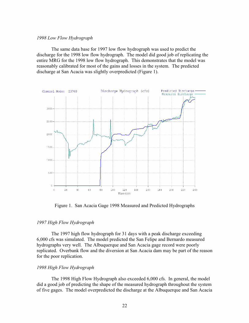
1998 Low Flow Hydrograph The same data base for 1997 low flow hydrograph was used to predict the discharge for the 1998 low flow hydrograph. The model did good job of replicating the entire MRG for the 1998 low flow hydrograph. This demonstrates that the model was reasonably calibrated for most of the gains and losses in the system. The predicted discharge at San Acacia was slightly overpredicted (Figure 1).

Figure 1. San Acacia Gage 1998 Measured and Predicted Hydrographs 1997 High Flow Hydrograph The 1997 high flow hydrograph for 31 days with a peak discharge exceeding 6,000 cfs was simulated. The model predicted the San Felipe and Bernardo measured hydrographs very well. The Albuquerque and San Acacia gage record were poorly replicated. Overbank flow and the diversion at San Acacia dam may be part of the reason for the poor replication.

1998 High Flow Hydrograph The 1998 High Flow Hydrograph also exceeded 6,000 cfs. In general, the model did a good job of predicting the shape of the measured hydrograph throughout the system of five gages. The model overpredicted the discharge at the Albuquerque and San Acacia

22

gage and underpredicted the discharge at the Bernardo and San Marcial gages. Based on the previous calibration runs, it was considered inappropriate to increase or decrease the infiltration losses to create a better match.

2001 Hydrograph The 2001 hydrograph represented a block release of about 4,000 cfs over a two day period. This block release would have been an excellent model test except for the additional Jemez Dam release whose hydrograph was not very well monitored. A one hour time lag was assumed for the Jemez release to arrive at the Rio Grande. The combined peak discharge exceeded 6,000 cfs. The 2001 flood pulse was accurately replicated for the San Felipe (Figure 2) and reasonably reproduced the hydrograph shape at Bernardo and San Acacia. The replication was poor at the Albuquerque and San Marcial gages.

Figure 2. San Felipe Gage 2001 Measured and Predicted Hydrographs Overall the model did a reasonably good job of replicating the five calibration hydrographs. One or more gages are poorly replicated for each hydrograph. The San Acacia and San Marcial gages had the poorest replication followed by Albuquerque and Bernardo. The two gages at the lower end of the system are subject to vagaries of the sand bed channel and constant gage shifts.

23

AMAFCA Overbank Flooding Model Overbank flooding on the Rio Grande floodplain between the North Diversion Channel and the I-40 Bridge in Albuquerque was predicted using the FLO-2D flood routing model. AMAFCA requested that the FLO-2D model be used to analyze potential flooding on this reach of the floodplain with a focus on the area near Montano Bridge. The MRG FLO-2D model with the 500 ft grid system was applied to the study reach by specifying new inflow and outflow locations. The model predicted the overbank flood inundation for five prescribed hydrographs. Flood hazard maps were prepared that displayed the predicted maximum flow depths for each flood scenario using aerial photographs as a background. The model modifications that were made for this study include:

• Six recently surveyed cross sections were added to improve channel geometry resolution;

• Global adjustment of the floodplain roughness was made to reflect the dense understory vegetation;

• Individual floodplain grid element roughness was adjusted near the Montano Bridge site based on aerial photos and site inspection;

• The west side levee was extended east at Montano Bridge to show the narrowing of the floodplain caused by the bridge approach embankment.

Bureau of Reclamation Levee Failure Project The goal of this project was to produce digital, geo-referenced flood inundation maps near Bernalillo for a hypothetical levee failure at two sites south of the New Mexico State Highway 44 Bridge. A 200 ft grid system was created from mapping developed from aerial photogrammetry exposed in April of 2000. The CADD files have two foot contours and are published at a 1”= 200’ horizontal scale. All of the data was referenced to the New Mexico State Plane Coordinate Grid System central zone NAD 83. In addition to the digital mapping, 21 Bernalillo Bridge (BB) lines on the Rio Grande surveyed in May, 2003 were used to create the channel component of the FLO-2D model. This channel database was supplemented with three additional BB lines surveyed in May 2001. The 200-ft grid system resulted in 4,850 grid elements and 117 channel elements. Each grid element represented just less than 1 acre. The hydraulic roughness n-values for the channel elements ranged from 0.026 to 0.030. Channel infiltration or surface water evaporation was not simulated because the losses were assumed to be minimal in this reach. The East Side Rio Grande levee crest elevations were determined from the DTM data.

Three hydrographs, representative of peak flows in the range of the 2 to 25 year recurrence interval flood (post-Cochiti data) were developed to simulate potential levee failure on the East Side of the river. The simulated hydrographs did not result in water surface elevations that exceeded the levee crest and levee failure was assumed to occur

24

due to levee sloughing or lateral bank erosion. Without simulating levee failure, the floods for the three hydrograph scenarios were contained by the Rio Grande levee through the entire study reach. When levee failure was simulated at the sites, substantial shallow, low velocity flooding was predicted to occur outside the levee near Bernalillo. At both levee failure sites the discharge through the levee flowed in a southerly direction. It was noted that the failure scenario (complete levee failure with the flow inundating the toe of the levee) inundated the maximum area outside the levee because the levee was presumed to fail at the earliest possible moment in the floodwave passage past the levee failure site. Rio Grande Model Upstream of Cochiti Reservoir Two additional Rio Grande reaches were modeled in conjunction the URGWOPs planning effort. The FLO-2D models were developed by Tetra Tech ISG. The first reach extended from the Rio Chama confluence to Cochiti Reservoir. This model had 98 surveyed cross sections and used 500 foot grid elements. There were no tributary inflows to the reach. The second model encompassed the Rio Chama reach from Abiquiu Dam to the confluence with the Rio Grande. There were 49 cross sections surveyed in March of 2003 upstream of San Juan Pueblo and 18 cross sections surveyed in February 2001 on San Juan Pueblo. The grid element size for this project was smaller (200 feet). The tributary inflow in the model was the Ojo Caliente. San Acacia Reach Levee Hydrology The Rio Grande Floodway Unit Flood Damage Reduction Project from San Acacia to San Marcial is a reevaluation of a Corps of Engineers flood protection project. The length of the project area is approximately 49 river miles. Proposed project features include: 1) Engineered levees on the west side of the Rio Grande floodway; 2) A sediment control area at Tiffany; and 3) Relocation of the railroad bridge at San Marcial.

To estimate peak discharge for this project, a flood flow frequency analysis at San Acacia was conducted by the Corps of Engineers. The San Acacia gage data was adjusted to account for upstream reservoir flow regulation. To compute flood frequencies at downstream locations, return period flood hydrographs were routed downstream using FLO-2D model to simulate the potential overbank flooding during the selected storm events. The Cochiti Dam to Elephant Butte MRG FLO-2D model was applied, but the inflow hydrographs were input to the model at the Bernardo gage, Rio Puerco and Rio Salado corresponding channel elements. The FLO-2D model for peak flow events from the Rio Salado show that attenuated peak flows are consistent with corresponding recorded peak flow events at San Acacia. The results of routing peak flow hydrographs were reported at selected locations. The levee data used in the FLO-2D model was modified to represent with-project conditions. The FLO-2D model proved to be a good tool for flood routing. The Corps reported that FLO-2D was a valuable model for estimating the effects of floodwave attenuation due to overbank flows and that it proved useful in predicting the combined inflows from several flow sources.

25

Save Our Bosque Conceptual Restoration Plan – San Acacia to San Marcial The goals of the Save Our Bosque Conceptual Restoration Plan are to enhance natural river functions and increase biological habitat diversity of the Rio Grande in the reach from San Acacia to San Marcial. The plan embodies several key elements of natural river processes including: channel forming flows of a prescribed frequency and duration; an active channel with limited vegetation encroachment; a hydrologic connection between river and floodplain that will regenerate native riparian vegetation and sustain wetlands and marshes; and a dynamic river system that has capacity to respond to large flood events. The FLO-2D model was used to determine the floodplain inundation for the different plan scenarios. First the MRG FLO-2D model was recalibrated to the previous 1992 BOR mapping previous discussed. It was not possible to replicate the 1992 mapping and San Marcial discharge exactly as had been done in the past because the current cross sections in the model were narrower. Calibration of the model was focused on adjusting the infiltration and n-values to approximate the 1992 area of inundation. The calibrated base model was modified to create an existing conditions model. The BOR new pilot channel in the Bosque del Apache NWR was added to the model. The channel roughness n-values were increased by 20 to 25% to reflect the increase in vegetation encroachment in the active channel. Spatially variable floodplain roughness n-values were assigned using the vegetation shape files for the mapped vegetation classifications sub-types. The shape data files were imported to the GDS processor program with the overlaid FLO-2D grid system and the vegetation n-values were interpolated and assigned to each grid element in the project reach. Grid elements with two or more vegetation shape file polygons were assigned n-values that were weighted proportionately the interpolation computation. These changes constituted the existing condition model. The existing conditions FLO-2D model was then revised to represent the proposed restoration projects. The original channel roughness n-values used in the calibrated base model were restored to the model data files based on the assumption that channel maintenance involving disk and mowing would keep the active channel free of vegetation. The restoration channel roughness would be lower than that in the existing conditions model. Floodplain roughness n-values were assigned in a similar manner to the vegetation interpolation for the existing conditions. The project shape files were assigned representative n-values that were significantly lower than those associated with the dense riparian existing conditions. Each restoration activity shape file polygon was assigned an n-value that was interpolated by the GDS processor program and assigned to individual FLO-2D grid elements. The final modification to the FLO-2D model to simulate flooding for the proposed restoration plan was to represent the physical changes to the river channel geometry. Each subreach had several significant channel enhancement projects. These are listed in Table 7 along the with the affected FLO-2D grid elements.

26

The application of FLO-2D indicates there would be a net decrease in infiltration and evaporation with the long-term comprehensive plan. Most of the reduction in floodplain inundation occurs in the reach from the new BOR pilot channel to San Marcial. In turn, more channel-floodplain hydrologic connectivity is prescribed for the Escondida and San Antonio reaches. During a feasibility level study, the actual restoration design will be tested and the final net salvage or depletion volumes will be computed.

TABLE 7. RESTORATION COMPONENT FLO-2D MODEL REVISIONS Project ID Approximate Location Affected

Grid Elements

Model Revisions

Escondida Subreach Eb1 4 miles downstream of S.A. diversion 24286-24367 Lowered right bank elevation and widened

channel by 500 ft Eg1 4 miles downstream of S.A. diversion 24284-24354 Secondary channel, lowered floodplain

elevations Ee1 5 miles downstream of S.A. diversion 24387-24584 Lowered bank elevation and cut channel

bank back 50 ft Ee2 and Eg2 5 miles upstream of Escondida Bridge,

near cross section SO-1280 24629-24735 Lowered floodplain elevations 1-2 ft to create secondary channel, lowered bank elevations by 4-5 feet

Ej1 and Ej2 Ej1 near cross section SO-1280 Ej2 near cross section SO-1299

24667-24696 24816-24843

Grade control structures, raised bed 2 ft and increase slope for 1,500 ft downstream

San Antonio Subreach Sg1 0.5 miles downstream of the North

Socorro Diversion Channel 25052-25090 Lower floodplain elevations by 1-2 ft to create secondary channels

Se1 and Sb1 5 miles downstream of the North Socorro Diversion Channel near Arroyo del Tajo

25285-25393 Lowered bank elevation and floodplain by1 ft and reworked the channel banks

Sb2, Sb3 Extends from Browns Arroyo to 1.5 miles upstream of Hwy 380 Bridge 25451-25828 Destabilized banks, revised bank slopes

Sb4 Extend from 0.25 miles downstream of Hwy 380 Bridge to about cross section SO-1496, about 1.25 miles

26001-26129 Destabilized banks, revised bank slopes

Se2 and Se3 1 mile upstream of the north boundary Bosque del Apache NWR 26184-26233 Lowered floodplain and island area by 1-3 ft

Refuge Subreach Rf1, Re1 and Rg1 0.5 mile downstream of the north

boundary Bosque del Apache NWR 26332-26464 Created a new channel using cross section 1508.9, used old channel as backwater habitat, lowered banks and floodplain 1-2 ft

Rh1 1.0 mile downstream of the north boundary Bosque del Apache NWR 26450-26496 Enhanced wetland area, lowered floodplain

elevations 1-2 ft, created drainage Re2 2.0 miles downstream of the north

boundary Bosque del Apache NWR 26517-26557 Lowered island/bar and left bank by 1-3 ft

Rg2, Rg3 and Rh2 3.0 – 5.0 miles downstream of the north

boundary Bosque del Apache NWR 26564-26774

Created secondary channels by lowering floodplain 1-3 ft, enhanced wetlands by lowering floodplain elevation 1-2 ft and creating drainage

Rb1 3.0 – 6.0 miles downstream of the north boundary Bosque del Apache NWR 26564-26890 Widen channel by 100 ft,

Rd3 and Re3 4.0 – 3.0 miles upstream of the south boundary Bosque del Apache NWR 26902-26988 New BOR channel was added, lowered

floodplain 1-2 ft, widened channel 100 ft Re4, Re5, Re6, Re7, Re8 and Re9

From 2.0 miles upstream of the south boundary Bosque del Apache NWR to 0.75 miles upstream of the San Marcial Bridge

26995-28300

Widened channel by using cross section SO-1667 to represented new channel geometry, widen channel to 360 ft in some locations. Left narrow channel in reaches of existing preferred vegetation.

Rh4 0.75 miles upstream of the San Marcial Bridge 28338-28518 Enhanced wetland area, lowered floodplain

elevations 1-2 ft, created drainage

27

MRG FLO-2D Model Components Introduction A number of FLO-2D model enhancements have been developed in conjunction with the Middle Rio Grande model. These include recent improvements to the GDS and MAPPER. The improvements to these two processor programs are extensive and are listed in Appendix A along with some of recent FLO-2D model revisions. Other enhancements to the FLO-2D model include an evaporation component, irrigation return flows, expanded spatially variable infiltration parameters, depth variable n-value adjustments, sediment transport, and output file details. A brief description of each new component is discussed. Evaporation An estimate of free surface evaporation was coded into the FLO-2D model for the Middle Rio Grande projects. Previously, channel and floodplain infiltration were the only losses that were computed in the model. The objective of adding the evaporation component was to separate the evaporation from the infiltration loss when calibrating the model. The infiltration loss can then be assumed to be either an increase in groundwater storage or potential loss to plant evapotranspiration. The FLO-2D model tracks the water surface area for both the channel and the floodplain on a timestep basis. To calculate the evaporation loss, the user must specify a mean monthly evaporation (in inches/month or mm/month if using metric units) in the INFIL.DAT file. The only other data requirement is the clock time at the start of the simulation. James Cleverly of the Department of Biology, University of New Mexico provided estimates of the percentage of daily evapotranspiration on an hourly basis for each month (Table 8). The evaporation loss is assumed to be constant during the hour shown in the table. The evaporation loss is reported at the end of the BASE.OUT and SUMMARY.OUT files in terms of both total evaporation in inches and total volume loss in acre-ft or cubic meters. A mean monthly evaporation for each month was derived from various sources such as the Rio Grande Joint Investigation General Report. For example: The mean monthly evaporation for Elephant Butte 1917-1936 for May: 12.77 inches The mean monthly evaporation for Albuquerque 1926-1932 for May: 10.73 inches The average for the two records was approximately 11.75 inches. A mean monthly evaporation of 8.22 inches was used in the FLO-2D model for May using a pan evaporation coefficient of 0.7. The mean monthly evaporation for the rest of the months were derived in a similar manner.

28

Table 8. Average Hourly Evaporation/ET

for 4 MRG ET Towers for May Hour Percent of Daily ET

12 – 1 am 1.0 1 – 2 am 0.0 2 – 3 am 0.0 3 – 4 am 0.0 4 – 5 am 0.0 5 – 6 am 0.0 6 – 7 am 0.0 7 – 8 am 2.0 8 – 9 am 5.0

10 – 11 am 6.0 11 – 12 pm 8.0 12 – 1 pm 10.0 1 – 2 pm 11.0 2 – 3 pm 11.0 3 – 4 pm 11.0 4 – 5 pm 10.0 5 – 6 pm 8.0 6 – 7 pm 7.0 7 – 8 pm 5.0 8 – 9 pm 2.0 9 – 10 pm 1.0

10 – 11 pm 1.0 11 – 12 am 1.0

Irrigation Diversion Return Flows A modification to the FLO-2D model was made to simplify the simulation of diversions and return flows to the model. Previously, diversions were made by creating a tributary or diversion channel and assigning a hydraulic structure to the diversion channel to control the flow. The diversion channel also had to have an outflow node to discharge flow from the grid system. The model was modified such that inflow hydrographs to the channel could be assigned as either inflow or outflow hydrographs. A new variable was created to identify whether the hydrograph is an inflow to or outflow from the channel. In this way, simple diversions can be structured anywhere in the channel. No diversion structure or tributary channel is necessary. An outflow hydrograph can be created with as few as two or three hydrograph pairs if a constant flow is required. The diversion outflow hydrograph is limited to the flow in the channel such that if a diversion of 500 cfs is specified and there is only 300 cfs in the river channel, the diversion will be 300 cfs and the flow in the river channel will be set to zero. In the existing model, irrigation diversions are specified for Angostura, Isleta and San Acacia diversion dams. There is also a diversion from Cochiti Dam that is not included in the Cochiti gage data. Based on collaboration with the Middle Rio Grande Conservancy District (MRGCD), return flow locations were identified. For the

29

replication of historic flow events, the Angostura and Isleta Diversion return flows can be estimated as follows:

TABLE 9. MRG FLO-2D MODEL DIVERSIONS AND RETURN FLOWS

Diversion or Return Flow Diversion or Return Approximate Discharge (cfs) Approximate Location

(grid element) Cochiti Diversion Diversion 2001 60

UCRDR Return 50 2290 ATRDR Return 50 8972 SANWW Return 30 1837 ARSDR Return 70 9000 CENWW Return 75% of Angostura Diversion2 4883 LPIDR Return 50 16447

PERWW Return 25 15785 UN7DR Return 50% of Isleta Diversion 23209 LSJDR Return 40% Isleta Diversion 22227

Angostura Diversion Diversion Variable 1198 Isleta Diversion Diversion Variable 9334 LFCC Diversion Diversion Variable 23762

Albuquerque Diversion Diversion Variable 2349 1Cochiti Diversion was assumed to be a constant 200 cfs with an 80% return flow. This 160 cfs is added to the Angostura Diversion for computing the return flow in the Central Avenue Waste Way. 2CENWW is assumed to be 75% of the total Angostura Diversion plus the 160 cfs by-pass from Cochiti Diversion.

There are a number of small irrigation return flows that combined may total additional 50 to 100 cfs that are not accounted for in the model. As more data is made available by MRDCD, more return flows can be added to the model. In the FLO-2D simulations for the 40-year URGWOM planning model, these diversions and returns are consolidated within the reaches. The diversion and return flow discharge data is provided by the URGWOM planning team for the various 40-year operation model alternatives. In addition, a diversion for the Albuquerque drinking water project has been added to the model for the URGWOPs study.

Depth Variable Roughness The Middle Rio Grande has significant variability in bed form roughness from lower regime to upper regime sediment transport as the flow approaches bankfull discharge. Upper regime plane bed can occur at a location for one discharge and not occur at a later time at the same location and same discharge. If the flow regime transitions from dunes to upper regime plane bed, the hydraulic roughness can decrease by as much as 50%. To simulate this effect and improve the timing of floodwave progression through the system, a depth variable roughness component was added to the model. It can be assigned on a reach basis. The basic equation is for the channel element roughness nd as function of flow depth is: nd = nb rc e-(r2 depth/dmax) where:

nb = bankfull discharge roughness depth = flow depth dmax = bankfull flow depth r2 = roughness adjustment coefficient prescribe by the user (0. to 1.2)

30

rc = 1./e-r2

This equation provides that the variable depth channel roughness is equal to the bankfull roughness at bankfull discharge. If the user assigns a roughness adjustment coefficient value (r2 = 0 to 1.2) for a given reach, the roughness will increase with a decrease in flow depth; the higher the coefficient, the greater that the increase in roughness. This roughness adjustment will slow the progression of the floodwave advancing down the channel by increasing the roughness for less than bankfull discharge. The roughness set for bankfull discharge will not be affected. For example, if the depth is 20% of the bankfull discharge and the roughness adjustment coefficient is set to 0.444, the hydraulic roughness Manning’s n-value will be 1.4 times the roughness prescribed for bankfull flow. Sediment Transport FEMA FIS studies are usually conducted using a rigid bed hydraulic model such as the Corps of Engineers HEC-RAS model. When a channel rigid bed analysis is performed, potential cross section changes are assumed to have a negligible effect on the predicted water surface. This is a reasonable assumption for large flood events on the order of a 100-year flood. To address mobile bed issues, FLO-2D has a sediment transport component that can compute sediment scour or deposition. Within a given grid element, sediment transport capacity for total load is computed for either channel flow or overland flow based on the flow hydraulics. The sediment transport capacity is then compared with the sediment supply and the resulting sediment excess or deficit is distributed over the floodplain or channel bed surface. Sediment continuity is tracked through the system on a grid element basis. The maximum scour, deposition and final bed elevations are recorded in output files.

The sediment transport capacity is computed using a choice of seven possible equations for alluvial channels including Zeller and Fullerton, Yang’s equation, Ackers and White, Englund and Hansen, Laursen, Toffeleti, or Woo. Each sediment transport equation was developed to simulate specific channel or bed material conditions and has unique attributes that may limit their applicability to certain river reaches. In the FLO-2D model, the total load equations are used to compute the sediment transport capacity based on the predicted flow hydraulics between grid or channel elements. The sediment transport is uncoupled from the flow hydraulics. First, the flow hydraulics are computed for all the floodplain grid and channel elements for the given time step and then the sediment transport is computed based on the completed flow hydraulics for that timestep. This assumes that the change in channel geometry resulting from deposition or scour does not have a significant effect on the average flow hydraulics for that timestep. Generally it takes several timesteps on the order of 10 seconds to result in average sediment deposition or scour that exceeds 0.05 ft. Each sediment transport equation is briefly described. It should be noted that each equation may have significant limitations that should be observed. When reviewing

31

the SEDTRANS.OUT file, it can be observed that for river flow the Ackers-White and Engelund-Hansen equations generate the highest sediment transport capacity; Yang and Zeller-Fullerton result in a moderate sediment transport quantities; and Laursen and Toffaleti compute the lowest sediment transport capacity. The Woo equation was added to the model to simulate the sediment transport in steep tributary channels and basins. For further discussion on the sediment transport and for references please consult the FLO-2D manual.

Ackers-White Method. Ackers and White expressed sediment transport in terms

of dimensionless parameters based on Bagnold’s stream power concept. They proposed that only a portion of the bed shear stress is effective in moving coarse sediment. Conversely for fine sediment, the total bed shear stress contributes to the suspended sediment transport. The series of dimensionless parameters include a mobility number, representative sediment number and sediment transport function. The various coefficients were determined by best-fit curves of laboratory data involving sediment size greater than 0.04 mm and Froude numbers less than 0.8. The condition for coarse sediment incipient agrees well with Sheild’s incipient motion criteria. The Ackers-White approach tends to overestimate the fine sand sediment transport.

Engelund-Hansen Method. Bagnold’s stream power concept was applied with the

similarity principle to derive a sediment transport function. The method involves the energy slope, velocity, bed shear stress, median particle diameter, specific weight of sediment and water, and gravitational acceleration. In accordance with the similarity principle, the method should be applied only to flow over dune bed forms, but Engelund and Hansen determined that it could be effectively used in both dune bed forms and upper regime sediment transport (plane bed) for particle sizes greater than 0.15 mm.

Laursen’s Transport Function. The Laursen formula was developed for

sediments with a specific gravity of 2.65 and had good agreement with field from small rivers such as the Niobrara River near Cody, Nebraska. For larger rivers the correlation between measured data and predicted sediment transport was reportedly poor. This set of equations involved a functional relationship between the flow hydraulics and sediment discharge. The bed shear stress arises from the application of the Manning-Strickler formula. The relationship between shear velocity and sediment particle fall velocity was based on flume data for sediment sizes less than 0.2 mm. The shear velocity and fall velocity ratio expresses the effectiveness of the turbulence in mixing suspended sediments. The critical tractive force in the sediment concentration equation is given by the Shields diagram.

Toffeleti’s Approach. Toffaleti develop a procedure to calculate the total

sediment load by estimating the unmeasured load following the Einstein approach. The bed material load is give by the sum of the bedload discharge and the suspended load in three separate zones. Toffaleti computed the bedload concentration from his empirical equation for the lower-zone suspended load discharge and then computed the bedload; whereas in the Einstein approach, the bedload is determined first, then the suspended load is computed through integration. The Toffaleti approach requires the average velocity in

32

33

the water column, hydraulic radius, water temperature, stream width, D65 sediment size, energy slope and settling velocity. Toffaleti’s procedure was satisfactorily applied for a large set of river and laboratory data.

Yang’s Method. Yang determined that the total sediment concentration was a

function of the potential energy dissipation per unit weight of water (stream power). The stream power was expressed as a function of velocity and slope. The total sediment concentration was expressed as a series of dimensionless regression relationships. The equations were based on measured field and flume data were made for sediment particles ranging from 0.137 mm to 1.71 mm and for flows depths from 0.037 ft to 49.9 ft. The majority of the data was limited to medium to coarse sands and flow depths less than 3 ft. Yang’s equations in the FLO-2D model can be applied to sand and gravel.

Zeller-Fullerton Equation. Zeller-Fullerton is a multiple regression sediment

transport equation for sand bed channels or alluvial floodplains . This empirical equation is a computer generated solution of the Meyer-Peter, Muller bed-load equation applied in conjunction with Einstein’s suspended load integration (Zeller and Fullerton, 1983). The bed material discharge qs is calculated in cfs per unit width as follows:

qs = 0.0064 n1.77 V4.32 G0.45 d-0.30 D50-0.61

where n is Manning’s roughness coefficient, V is the mean velocity, G is the gradation coefficient, d is the hydraulic depth and D50 is the median sediment diameter. All units in this equation are in the ft-lb-sec system except D50, which is in millimeters. If the metric option is activated, no unit conversions are necessary. For a range of bed material from 0.1 mm to 5.0 mm and a gradation coefficient from 1.0 to 4.0, this equation should be accurate with 10% of the combined Meyer-Peter Muller and Einstein equations. The Zeller-Fullerton equation assumes that all sediment sizes are available for transport (no armoring). The original Einstein method is assumed to work best when the bedload constitutes a significant portion of the total load. Woo. Woo’s equation for computing bed material load in channels with high sediment concentrations of suspended sediment was coded into the model to compute sediment supply from steep tributary channels and basins. In 1993, Mussetter combined Woo’s 1985 relationship with the Meyer-Peter Muller bedload equation to develop a sediment supply equation as a power function of the velocity, depth, sediment size D50, and fine sediment concentration for the steep watersheds around Albuquerque. The equation is limited to bed layer concentrations less than 650,000 ppm by weight. This equation should be used for steep channels with highly erodible material. It will generate a sediment load that is one to two orders of magnitude higher than the other sediment transport equations previously discussed. Summary. In the absence of measured data, the application of the total load sediment transport formulas are recommended as follows:

34

• Use Meyer-Peter and Muller and Einstein procedure (Zeller and Fullerton equation) when the bedload is a significant portion of the total load.

• Use Toffaleti’s method for large sand-bed rivers. • Use Yang’s equation for sand and gravel transport in natural rivers. • Use Ackers-White or Engelund-Hansen equations for subcritical flow in lower

sediment transport regime. • Use Laursen’s formula for shallow rivers with silt and fine sand. • Use Woo’s equation for steep alluvial tributary channels.

It is important to note that in applying these equations, the wash load is not included in the computations. The wash load should be subtracted from any field measurements before comparing with the predicted sediment transport results from the equations. It is also important to recognize if the available field measurements are supply limited. If this is the case, the comparison of field measurements with the sediment transport capacity equations would be inappropriate. Depth Duration To address issues associated with the URGWOPs EIS regarding overbank flooding; a depth duration analysis was coded into the model. An input data parameter is assigned a depth value (typically 0.5 ft.) and the FLO-2D model then computes the duration in hours that this depth is exceeded by the floodplain inundation. This computation is made on a grid element basis and can be plotted graphically with the MAXPLOT processor program. For a given spring runoff hydrograph, the depth duration in hours can be displayed to identify areas of the floodplain where the flood inundation is sufficient to support the riparian ecology in terms of flushing forest litter, nutrient recycling, and cottonwood/willow bosque regeneration. The depth duration delineation can also support the prediction of slow floodplain velocity habitat for the silvery minnow. Channel Hydraulics The analysis of average channel hydraulics was expanded to include thalweg depth, flow velocity, discharge, water surface slope, bed slope, energy slope, bed shear stress, wetted perimeter, top width, hydraulic radius, width-to-depth ratio, and water surface elevation. This output data was written to file for a range of discharges. It can then be analyzed on a grid element basis or over several grid elements in the HYDROG post-processor program. The FLO-2D model was used to simulate steady flow, discharge increments of three to five days to generate the output data files that can be interpolated with the HYDROG program. HYDROG provides the opportunity to select a reach of river and a given discharge to compute the average flow hydraulics in the reach. The average flow hydraulics for a selected discharge are computed by interpolating discharge weighted and reach length weighted average hydraulic conditions. The reach average hydraulics can be computed for any selected discharge ranging from 25 cfs to 10,000 cfs assuming that the selected discharge can be conveyed by the channel at the reach

35

location. This channel hydraulic data can be useful in accessing silvery minnow and other aquatic habitat as function of discharge. Overbank Flooding When overbank flooding is initiated in a given grid element, the simulation time (in hours) is written to an output file along with the grid element number, the channel cross section, the thalweg flow depth, velocity, discharge and water surface elevation. The volume of water (in acre-ft) on the floodplain for the whole river system is also reported in the same file. The 40-year URGWOM planning model alternative scenarios provide a wide range of spring flood hydrographs with variable peak discharge magnitude, duration and timing. With floodwave attenuation associated with both channel and overbank storage, the movement of the peak discharge and the corresponding time of initial overbank discharge through the system is highly variable. Overbank discharges can be initiated at different times in different locations for the same Cochiti Dam peak discharge release. The location of initial overbank flooding can be correlated with flood frequency, habitat value and other parameters. This overbank flood information is also provided on a reach basis using the URGWOPs delineation of MRG reaches.

36

MRG FLO-2D Model Limitations and Potential Improvements Introduction The FLO-2D model will be expanded in the future to include more detail of the channel-floodplain flooding interface along the Middle Rio Grande. At the present time, the primary limitations of the MRG FLO-2D model are related to:

• Grid element size • Floodplain spatially variable roughness and infiltration parameters • Model calibration for high flows • Modeling details • Sediment transport • Simulation time

Each of these issues will be briefly discussed as it relates to MRG flood simulation. Grid Element Size The grid element size of 500 ft (5.74 acres) for the MRG model (30,000 grid elements) provides sufficient resolution for large flood events. A tradeoff was made between more floodplain resolution and longer model run times. Each grid element is represented by only one elevation and roughness. Shallow flooding less than 0.5 ft has limited accuracy. Small rills and gullies that may exist along rangelines (often trampled by cattle) may initiate a limited amount of overbank flooding before general flooding occurs on the grid element. Floodplain elevation variability of several feet within a grid element would probably result in several ponded and dry areas. If a grid element is predicted to have flood inundation, it is likely that there will be some flooding somewhere on the element. With grid elements of this size, the initial time and location of overbank flooding has to be viewed with perspective that a minimum of several grid elements should be inundated to verify that overbank flooding has begun. If more resolution is necessary for a given project, a smaller grid system can be considered for a short reach of river.

Floodplain Spatially Variable Roughness and Infiltration Parameters One MRG FLO-2D model attribute that can be improved in the near future is spatially variable floodplain roughness and infiltration parameters. Spatially variable roughness was assigned for the reach from San Acacia to San Marcial using the GDS and available vegetation mapping. The majority of the remaining Rio Grande floodplain has been assigned a uniform roughness n-value of 0.065. As more floodplain vegetation mapping is made available, spatially variable roughness can be assigned based on vegetation types. If vegetation shape files are available, n-values can be assigned to shape polygons and the GDS can import the shape files and interpolate roughness values to the grid element. This is an efficient process. The infiltration parameters can be

37

High flow model calibration has been planned for the past couple of years. An overbank flooding report prepared by Tetra Tech was submitted to the MRG ESA Collaborative Program (through the Corps of Engineers) that outlines a high flow data collection program to calibrate the MRG FLO-2D model. Without the high flow calibration, the area of inundation can not be predicted with certainty. At the present time this is the most significant limitation associated with the MRG FLO-2D model. The recommended high flow data collection effort will be designed to maximize the data collected during the limited high flow duration. Aerial photos will be used to estimate the area of inundation. Ground surveys and observations will compliment and verify the aerial photography and videos. Channel cross section and high water surface elevation surveys will identity the channel geometry response to high flows and will enable additional calibration of channel hydraulic roughness in the model. Discharge measurements will verify the accuracy of USGS gage calibration and will help to assess floodwave attenuation. As a suggestion, a model calibration test release from Cochiti Dam could be considered for the non-irrigation season. The test release would be only for in-channel calibration (less than 3,500 cfs) for about three days. It would be used to calibrate the channel floodwave movement and attenuation.

assigned in a similar manner if soil maps are available as shape files. The GDS has an automated routine for interpolating all the Green-Ampt infiltration parameters used by the FLO-2D model. Model Calibration for High Flows

Discharge Measurements

Discharge measurements during calibration high flows should be considered to improve the accuracy of the gage record during the high flow releases. This discharge gaging effort can be coordinated with the USGS or field crews can collect the discharge measurements. Additional discharge measurement sites could be set up for the high flow event. Standard USGS discharge measurement methods would be followed. Accurate discharge data at San Marcial will be important for calibrating floodwave attenuation in the FLO-2D model. For discharge estimates at sites without a USGS gage, a level sensor can be installed in a PVC pipe. The level logger can be calibrated by taking a series of discharge measurements at the site.

Aerial Photos

Aerial photos or video should be taken of the entire MRG during a prescribed event. The primary purpose of any aerial photographic mission during high flow is to record or estimate the area of inundation as the floodwave moves downstream. There are two alternatives for the aerial photos, fixed wing aircraft and satellite imagery. The photography should be taken near the end of the high flow release. This will allow for maximum capture of floodplain inundation. The timing of the aerial photography should leave sufficient time to consider a second photographic set or backup flight if there are weather or mechanical problems. A digital aerial video of the reach should be taken for the purpose of analyzing flooding in specific reaches. A clear, comprehensive video of

38

the study reach would improve the calibration of the MRG FLO-2D model and its ability to predict floodplain areas of inundation.

High Flow Cross Section Surveys

Cross section surveys will assess changes in channel geometry during high flows. Almost all previous cross section surveys were done at low or moderate flows. Water surface elevation and bed forms will be recorded. Scour or deposition during high flows can be estimated by comparing the high and low flow cross section surveys. The cross section survey and local overbank flooding can be documented with ground photography.

River Channel Water Surface Elevation Surveys

River channel water surface elevation surveys will be used to calibrate the FLO-2D model n-values. Due to high flow hydrograph time limitations, not every cross section can be surveyed. For those cross sections where channel geometry is not surveyed, only the water surface elevation should be surveyed. Survey shots will be taken on one of the cross section endpoints and an adjacent water surface from which the water surface elevation will be calculated.

Overbank Flooded Areas

In floodplain locations where there are no cross sections, water surface elevations can be estimated from the levee with a GPS unit. Floodplain ground elevation data is available from existing DTM mapping or if necessary, it can be surveyed at a later time. The extent of the area of inundation will be estimated from the aerial photos or video. Levee bar and cap elevations can be used to calibrate the GPS unit in a floodplain reach. Ground photos of the area of inundation will complement the aerial photography.

Modeling Details Adding model detail will improve the resolution of the flood routing and overbank inundation. Suggested model enhancements include:

• Adding rating tables for bridges and other hydraulic structures. • Adding more return flows. • Adding drainage canals and associated berms. • Checking levee crest elevations.

These modeling improvements should be considered when budget and resources are available. They are secondary in importance to high flow calibration and spatially variable floodplain roughness. Sediment Transport Sediment routing by size fraction and armoring are being implemented in the FLO-2D model to compliment the addition of the new sediment transport equations. This will enhance channel morphology investigations in local project reaches. Adding more detail to the sediment transport component will improve the prediction of river response

39

to restoration activities. It will also help to evaluate the long term response to drought conditions or wet periods. Model Run Time It is a goal of the model development to decrease the computer run time of MRG FLO-2D model. Typical spring flood hydrograph simulations take 6 to 12 hours to complete. Improving the model algorithm speed is a high priority, but is generally relegated to secondary funding status.

40

How to Use the FLO-2D Model for MRG Projects The MRG FLO-2D model can be used to predict water surface elevations, areas of flood inundation and floodwave attenuation. Local reach studies may need some refinement based on levee heights and locations, floodplain elevations and floodplain roughness. Variation in floodplain infiltration should also be considered. Changes to the model data base should be undertaken when supporting data is available. In order to run the model for different flood events, it is only necessary to revise hydrographs in the INFLOW.DAT file. There are several suggestions that will facilitate using the model:

1) Make sure there is flow (base flow) in the Rio Grande channel before adding the side tributaries or irrigation return flows. This will eliminate the inflow from spreading upstream and slowing down the model Lag the inflows sufficiently to allow the upstream river flow to reach the tributary or return flow location.

2) Enhance the inflow hydrographs by adding more irrigation return flows, channel diversions or tributary flood events. Return flows should consider appropriate lag times to match the floodwave movement in the river.

3) Add more detail to levees, floodplain infiltration and roughness and return flows.

Changes to the data files should be documented and reported to the FLO-2D Workgroup and Tetra Tech. If you have changes that should be considered as a permanent revision to the model data files, these will be recorded and reported to others through the FLO-2D Workgroup. The FLO-2D Workgroup can serve as a repository for the baseline MRG model.

41

Summary The Middle Rio Grande FLO-2D model has been evolving since 1997 through its application to a number of flood projects. The development has been support by both federal and state agencies and has culminated in its application to support the URGWOPs EIS. A number of enhancements were made to the processor programs including the GDS, MAPPER, FLOENVIR, HYDROG and PROFILES to facilitate the model application to the MRG. A big step in this process was the conversion of the model to use the surveyed cross section data instead of the channel geometry relationships. This conversion made the model more stable and significantly decreased the MRG model simulation time.

The ISC supported the calibration of the MRG FLO-2D. There was a limited data base upon which to perform model calibration from Cochiti Dam to San Marcial. Suitability criteria for selecting hydrograph calibration data included available tributary inflow hydrographs, gaging data consistency, and hourly data. The focus of the calibration was hydrograph timing, shape and volume at the five gaging stations. The calibration effort included portions of the seasonal high flow hydrographs from the years 1997, 1998 and 2001. The primary parameters adjusted for the calibration included channel roughness and channel infiltration.

Calibration of the MRG model was difficult and time consuming because of the

of poor calibration of USGS gages, ungaged tributary inflow, ungaged irrigation return flows, and lack of hourly data. For each of the five selected hydrographs, the FLO-2D results replicated several of the USGS gage hydrographs fairly well. If the FLO-2D results for a specific gage displayed a poor replication of the gaged flow, it was likely that the gage rating curve had shifted. Overall, the calibration of the MRG FLO-2D model was relatively good.

Following the 2002 calibration effort, six MRG flood projects have been undertaken with the FLO-2D model. Three projects are essentially complete including the AMAFCA overbank flood study between the North Diversion Channel and the I-40 Bridge in Albuquerque, the Bureau of Reclamation simulated levee failure project, and the Save Our Bosque conceptual restoration plan for the San Acacia to San Marcial reach. The URGWOPs related projects on the Middle Rio Grande, Rio Chama and the reach between the Rio Chama and Cochiti Reservoir are still in progress.

Data collection activities in the Middle Rio Grande during a high flow release

from Cochiti Dam should be coordinated with the various agencies to maximize the opportunity to calibrate the MRG FLO-2D model for overbank flooding in the future. An overbank monitoring plan has been formulated and submitted to the Corps and the ESA Collaborative Program that is designed to optimize high flow data collection.

The most important data collection tasks of the overbank monitoring plan are the aerial photography (and video) of the area of inundation and the high water surface elevation surveys. Surveying some cross sections at high flow is also a high priority.

42

High flow cross section surveys can be compared with the low flow cross section surveys to determine the channel geometry response to high flow. A priority list of proposed cross section surveys was prepared for the overbank monitoring plan. The on-the-ground data collection effort during high flows will focus on peak flow water surface elevations that can be correlated with the aerial photography of the area of inundation. Refinement of the overbank monitoring plan should be a priority after a potential high flow release is identified. FLO-2D model enhancement for future MRG applications should be focused on model calibration, spatial variation of floodplain roughness and infiltration parameters and modeling details such as hydraulic controls and return flows. Sediment transport analyses will provide additional insight into channel morphology responses to restoration activities and long term trends in channel changes. Two long term enhancements to the MRG FLO-2D model involve grid element size and model run times. As computer resources evolve with 64 bit processors, more interest will be focused on run times for longer FLO-2D simulations. This will occur in concert with demands for higher floodplain grid element resolution. A 100 ft grid system would result in 750,000 grid elements and long flood simulations of 3000 hours would take a week or more. For that reason, future model enhancement should consider improvements to model stability criteria and computer run times.

Appendix

Version 2003.06 Enhancements

FLO-2D Version 2003.06 Enhancements

FLO-2D Version 2003.06 includes the following new tools and components. These are enhancements to Version 2001.06.

• GDS and Mapper now have integrated ESRI MapObject Controls. • GDS includes automated computation of Green-Ampt Infiltration parameters and

n-values from shape files and ASCII tables. • GDS and Mapper can retrieve and display geo-referenced images. • GDS and FLO-2D will format and utilize real-time rainfall data. • GDS can cut channel cross sections from a DTM. • GDS and Mapper can import ESRI shape file data such as land use, soil types,

and n-values. • GDS and Mapper can import ESRI ArcInfo ASCII grid files with terrain

elevations and NOAA rainfall isopluvial data. • GDS and Mapper can import as background multiple geo-referenced aerial photos

in various formats such as TIFF, BMP, JPG, etc. • Multiple ESRI ArcInfo ASCII grid files can be listed in a tile and index catalog

file and referenced to a user defined polygon. • Multiple image files like aerial photos can be listed in a tile and index catalog file

and referenced to a user defined polygon. • New multiple layer capability in GDS and Mapper. • Improved zoom and pan features in GDS and Mapper. • Spatially variable Green-Ampt infiltration parameters can be assigned to grid

elements based on soil and land use shape files in GDS. • Spatially variable Manning roughness coefficients can be assigned to grid

elements based on Manning shape files in GDS. • Spatially and time variable rainfall data can be computed and assigned to grid

elements based on multiple NOAA rain data files in GDS. • Channel cross sections can be cut from DTM points in GDS. • New GUI data input interface with a simplified format. • FLO-2D has an improved channel routing algorithm. • FLO-2D has simplified data files with a new format. • FLO-2D has five new sediment transport equations. • FLO-2D has nonuniform sediment distribution on cross sections. • FLO-2D computes free water surface evaporation. • Spatially variable rainfall and moving storms can be formulated in the

FLOENVIR for FLO-2D simulation. • FLO-2D can predict and simulate real time storm return estimates. • FLO-2D has new stage-time and hydraulic structure controls. • There is a new floodway routine. • FLO-2D Light package in GDS will facilitate getting started on a project. • Convert HECRAS channel cross sections in GDS. • FEMA map template can be plotted in Mapper. • Read HEC-1 output hydrograph files in GDS for hydrograph management. • FLOENVIR functions are being converted to GDS

• DTM points can be deleted in GDS and Mapper. • Define computational area with a polygon in GDS. • Infiltration is now simulated with Green-Ampt five parameter spatial variability. • Mapper now plots velocity vectors. • Mapper can perform profile cuts in topography and flow depth. • Flood animation can be viewed in Mapper.

New components scheduled for the first half of 2004 are: • Tabular reporting of results in Mapper. • Mapper will be used to estimate peak flow from cross sections. • Mapper will have a damage assessment routine. • Investigate a flood probability evaluation method using a Monte Carlo method. • Mapper will display sediment deposition/erosion. • GDS and Mapper will have *.TOP project data recovery. • Improved error checking. • GDS with have an ‘In-line’ help system. • Tutorials.