California Institute of Technology

Pasadena, California

2001

(submitted November 3 2000)

Thesis by

Sven Bossuyt

Microstructure andCrystallization Behavior

in Bulk Glass Forming Alloys

In partial fulfillment of the requirements for the degree of

Doctor of Philosophy

ii

© 2001Sven Bossuyt

all rights reserved

iii

Acknowledgements

Caltech is a remarkable place. I wish to thank everybody who helped make the

five years I spent as a graduate student here both fruitful and enjoyable.

First and foremost, my gratitude goes to Professor Bill Johnson for giving me the

opportunity to pursue my doctorate at Caltech. It has been a pleasure working

with him. Due to his exceptional intuition and quickness of thought, discussing

results and ideas with him always results in refreshing insights.

I also benefited from stimulating discussions, collaboration on experiments,

demonstrations of equipment, and general companionship provided by

Channing Ahn, Uta Bete, Peter Bogdanov, Jonathan Burrows, Claudine Chen,

Dale Conner, Rich Dandliker, Prof. Pierre Desré, Carol Garland, Stephen Glade,

Charles Hays, Adrian Hightower, Jörg Löffler, Mike Manley, Jan Schroers, Valerie

Scruggs, Ben Shapiro, Laura Sinclair, Andy Waniuk, and Chuk Witham, among

others.

Financial support was provided by the Belgian American Educational Foundation

and the U.S. Department of Energy (Grant No. DEFG0386ER45242).

Last, but not least, I must acknowledge the support of my family. My parents

have always encouraged their children to be curious and creative, and to believe

in themselves. My wife helps me to do this, and makes me happy.

iv

Abstract

The solidification microstructure in wedge-shaped castings of Cu-Ni-Ti-Zr glass

forming alloys is investigated, while the composition was systematically varied.

Near the critical thickness for glass formation, a spatially inhomogeneous

dispersion of nanocrystals is observed, where spherical regions contain a much

higher density of nanocrystals than the surrounding material. This microstructure

is inconsistent with the prevalent theories for crystallization in metallic glasses,

which predict a spatially uniform distribution of crystals.

The spatial localization of the nucleation density is attributed to a recalescence

instability. Linear stability analysis of the equations for heat flow coupled with

crystal nucleation and growth reveals that at low temperature recalescence can

occur locally, triggered by a small fluctuation in the early stages of the

crystallization process, because in deeply undercooled liquids the nucleation rate

increases with temperature. The localized recalescence events and their

interaction accelerate crystallization; consequently they are important in

determining the glass forming ability as well as the microstructure of these alloys.

The composition dependence of the critical thickness for glass formation,

determined from the observed microstructures, and in situ small angle scattering

results indicate that the crystallization occurs in several steps, involving

competing crystalline phases.

v

Contents

1. Introduction

2. Experimental Techniques

2.1. Alloying 7

2.2. Metal mold casting 11

2.3. Microstructure characterization 17

2.4. Annealing 19

3. Microstructure

3.1. Metallography 21

3.2. SEM 28

3.3. X-ray diffraction 30

3.4. TEM 32

3.5. Conclusions 35

4. Crystallization Kinetics

4.1. Classical nucleation and growth kinetics 37

4.2. Spatially localized nucleation 47

5. Alloy Development

5.1. Requirements for glass formation 54

5.2. Empirical optimization 59

6. Annealing

6.1. Experimental results 65

6.2. Discussion 68

7. Summary

vi

A. Appendices

A.1. Properties of Vit101 74

A.2. Solutions to the Fourier heat flow equation 75

A.3. Geometry of composition spaces 80

References

vii

Figures

induction melting apparatus 9

alloy compositions 10

injection casting setup 12

drawing of wedge mold 15

overview of wedge-shaped casting usage for sample preparation 16

optical micrograph of Cu48Ni8Ti34Zr10 wedge 22

optical micrograph of Cu47Ni8Ti34Zr11 (Vit101) wedge 23

size distribution of spherical features 24

variation of critical casting thickness with composition 27

SEM micrograph of Cu46Ni8Ti35Zr11 wedge 28

SEM micrograph of crystallized Cu48Ni8Ti33Zr11 alloy 29

variation of X-ray diffraction pattern with thickness 31

TEM micrograph of Cu46Ni8Ti35Zr11 sample with nanocrystals 34

temperature dependence of nucleation rate 40

experimentally determined TTT-diagram 45

temperature regimes for type I and type II recalescence 51

schematic non-equilibrium phase diagram of eutectic system 56

schematic illustration of ternary eutectic phase diagram 63

in situ SAXS data for Vit101 annealed at 665 K 66

in situ SAXS data for Vit101 annealed at 769 K 67

DSC traces of annealed Vit101 samples 69

evolution of Guinier radius from SAXS 71

viii

temperature profile evolution in a flat plate 78

temperature profile evolution at semi-infinite wall 79

geometry of composition spaces 82

1

1. Introduction

Definition of glass

In general, when a liquid is cooled, its free volume decreases, and the amount of

short range order increases. As a result the mobility in the liquid decreases, e.g.,

diffusion constants decrease and the viscosity increases [1]. The time scale for

changing the configuration of the liquid becomes longer. When this time scale

exceeds the time scale of the experiment, the material behaves more like a solid

than like a liquid. This transition, where the time scale for sampling the

configuration space of the liquid crosses over the time scale of the experiment, is

called the glass transition.

A glass is then defined as a liquid cooled below its glass transition temperature.

The glass transition behaves like a second order phase transition, but it is not

strictly a phase transition in the thermodynamic sense. The difference between

the glass and the liquid is an issue of kinetics rather than thermodynamics. In the

framework of statistical mechanics, the configuration spaces of the glass and the

liquid are fundamentally the same. The configuration space of the glass appears

smaller because ergodicity breaks down on the time scale of the experiment. A

glass is therefore, by its definition, not an equilibrium phase.

For most metals and alloys, the equilibrium state at room temperature is a

crystalline phase or a mixture of crystalline phases [2]. At high temperatures the

2

liquid is thermodynamically stable. Below the liquidus temperature there is a

thermodynamic driving force for crystallization, so the liquid is metastable.

Whether or not crystals form depends on the crystallization kinetics. Below the

glass transition temperature the liquid is still metastable, but the crystallization

kinetics are so sluggish that it would take essentially forever to form a crystal.

The requirement for forming a glass is therefore to be able to avoid crystallization

while cooling the liquid from above the liquidus temperature to below the glass

transition.

Glass formation

Since the crystalline phase introduces order which was absent in the liquid

phase, there can not be a catastrophic crystallization instability like there is for

melting. Crystallization must occur via a process of nucleation and growth. It is

not necessary to completely eliminate nucleation in order to make a glass; if the

crystallized volume fraction is below the detection limit inherent in the

experiment, the material is amorphous for all practical purposes. The cooling rate

necessary to achieve this depends on the nucleation and growth rates and their

temperature dependence.

In the absence of convection or some adiabatic cooling mechanism, the cooling

rate is limited by thermal conduction in the liquid, which scales with the square

of the smallest sample dimension [3]. As a result, a critical cooling rate for glass

formation corresponds to a critical thickness for glass formation. This critical

3

thickness for glass formation can be used to quantify the concept of glass forming

ability. It is directly related to the critical cooling rate for glass formation, but

easier to determine experimentally —except for very good glass formers, where

the critical thickness is large and the critical cooling rate not very difficult to

achieve.

Glass forming materials

The most familiar glass forming materials are ceramics, network silicates to be

exact. Crystallization kinetics in network silicates are so sluggish that glass can

be formed even at geological cooling rates [4]. The manufacture of household

objects from silicate glass dates back at least to 2500 B.C., although the

transparent variety is a much more recent development [5]. Network silicates are

ideal glass forming materials, because the rearrangement of the silicate chains

into a crystalline network is a very slow process.

Polymer melts also consist of a tangle of chains that is difficult to rearrange into a

crystal. In some polymers with an aperiodic molecular structure or where the

chains form a covalently bonded network it is not possible to form a crystal at all.

Even crystalline polymers usually have a highly non-equilibrium microstructure

with a significant volume fraction of an amorphous phase between crystals [6].

Many other ceramic and organic glasses have been found, but metallic glasses

remain somewhat of a novelty. Metallic glass was first produced from the melt in

1960 at Caltech [7] by splat quenching Au-Si alloys near the eutectic composition.

4

Many other alloys have been vitrified since then using rapid quenching

techniques [8-10]. The soft magnetic properties of Fe-B based glass ribbons

produced by planar flow casting have led to their use in a wide range of

industrial applications [11]. But the need for high cooling rates has nevertheless

placed constraints on scientific experiments and practical applications. The recent

discovery of bulk metallic glasses, such as La55Al25Ni20 [12],

Zr65Al7.5Ni10Cu17.5 [13], Zr41.2Ti13.8Cu12.5Ni10Be22.5 [14], Pd40Cu30Ni10P20 [15],

Zr58.5Nb2.8Cu15.6Ni12.8Al10.3 [16] and related alloys has enabled practical

applications as well as studies of previously inaccessible properties of

undercooled liquids.

The initial objective for this work was alloy development: finding the

composition with the best glass forming ability in a given alloy system. A

systematic study of glass forming ability as a function of alloy composition

would be undertaken with the dual aim of improving our understanding of the

requirements for making bulk metallic glasses and testing techniques for locating

the optimum composition in newly discovered families of glass forming alloys.

The Cu-Ni-Ti-Zr system was chosen for this work, because Cu47Ni8Ti34Zr11

(Vit101) [17] is known to be a relatively good glass forming composition, and the

system contains “only” 4 components*.

* The complexity of the optimization problem increases exponentially with the

dimensionality of the composition space, so systems with fewer components are more

amenable to a systematic alloy development process. This is discussed in detail under

“Empirical optimization” on page 59 and “Geometry of composition spaces” on

page 80.

5

The intention was to identify a critical casting thickness for glass formation,

measure how it changes with small changes in composition, extrapolate these

results to find a better glass forming composition, and repeat this process until a

local optimum was found. However, the microstructure at the critical casting

thickness and its composition dependence proved to be much more complex

than expected on the basis of prevalent theories concerning crystallization

behavior in glass forming alloys.

Microstructure and crystallization behavior

Paradoxically, this work about a non-crystalline form of matter deals almost

exclusively with crystallization. Glass formation can only occur if crystals do not

form. The glass forming ability of an alloy is therefore related more to the

properties of the crystalline phases that do not form, than to the properties of the

glass that forms. It is the crystallization behavior at the critical cooling rate, i.e., in

the limit where crystallization does not occur, that must be understood in order

to understand glass formation. The microstructure of samples that solidified at

cooling rates close to this critical cooling rate holds important clues to the

crystallization behavior.

Alloys with different compositions close to Vit101 were studied in this work, by

examining the solidification microstructure in samples where the cooling rate

varied along the sample. Chapter 2 describes the sample preparation methods

and experimental techniques that were used. Chapter 3 gives an overview of the

6

observed microstructures, with particular emphasis on the features of the

microstructure close to the critical cooling rate for glass formation. Chapter 4

starts with a presentation of the classical theory for crystal nucleation and

growth, pointing out its shortcomings and the discrepancies with the

microstructures described in chapter 3. An extension of this theory is then

proposed, introducing the concept of localized recalescence to resolve these

discrepancies. A discussion, within this framework, of the variations in

crystallization behavior with composition leads to chapter 5 about alloy

development. Finally, in chapter 6, results of in situ experiments on the

crystallization behavior during annealing of amorphous samples are presented

and discussed.

7

2. Experimental Techniques

2.1. Alloying

Starting materials

Ingots of a variety of alloys in the Cu-Ni-Ti-Zr system, with compositions close to

the bulk glass forming alloy Cu47Ni8Ti34Zr11 (Vit101) [17], were prepared by

induction melting the constituent elements under inert atmosphere. In order to

keep the oxygen content of the alloys as low as possible, the highest purity Zr and

Ti crystal bar available from Wah-Chang Teledyne, with <50 ppm oxygen, were

used. Cu and Ni were supplied by CERAC, item Nos. C-1131 and N-2009

respectively.

Induction melting procedure

A typical sequence of events for preparing an alloy by induction melting is

described below:

• The alloying elements are weighed out. Small pieces are cut off with wire cut-

ters or added to adjust the amount of each of the elements until the desired

alloy composition is obtained.

• Before melting, the alloying elements are cleaned by sonication in acetone and

then in ethanol.

8

• The elements to be alloyed and the titanium getter are arranged* on separate

troughs in the copper boat, which is placed inside the fused silica tube, as

shown in Fig. 2.1.

• The tube is evacuated to < mbar and backfilled with ultra high purity

(UHP, 99.9999%) argon. It is then evacuated to < mbar.

• The Ti getter is heated to approximately 800 °C (glowing red-hot) for 5 min.

Then the sample is heated slowly while monitoring the vacuum gauge read-

out.

• When no more outgassing is observed, the sample is allowed to cool down

and the tube is backfilled again with UHP argon.

• The Ti getter is heated red-hot again for 5 min and allowed to cool down. The

getter is checked for signs of oxidation and heated red-hot for another 5 min.

• The elements are then heated until they are all molten together.

• The crystallization of the alloy is observed while it cools down. The alloy is

molten again and kept molten for 15 min. If the crystallization behavior is dif-

ferent from the first time, the sample is molten again for a longer time and/or

at higher power until a consistent crystallization behavior emerges.

• The sample is allowed to cool down, removed from the apparatus and

weighed to check for any weight change.

* If all elements are alloyed at once, Ni and Zr are the last elements to melt completely. To

avoid having to melt the alloy for a long time, the elements were arranged with Ni and

Zr on one side, and Cu and Ti on the other side of the same trough in the copper boat.

The large exothermic heat of mixing of the Ni and Zr assured that these elements were

alloyed completely before the Cu and Ti were added.

1 2–×10

1 5–×10

9

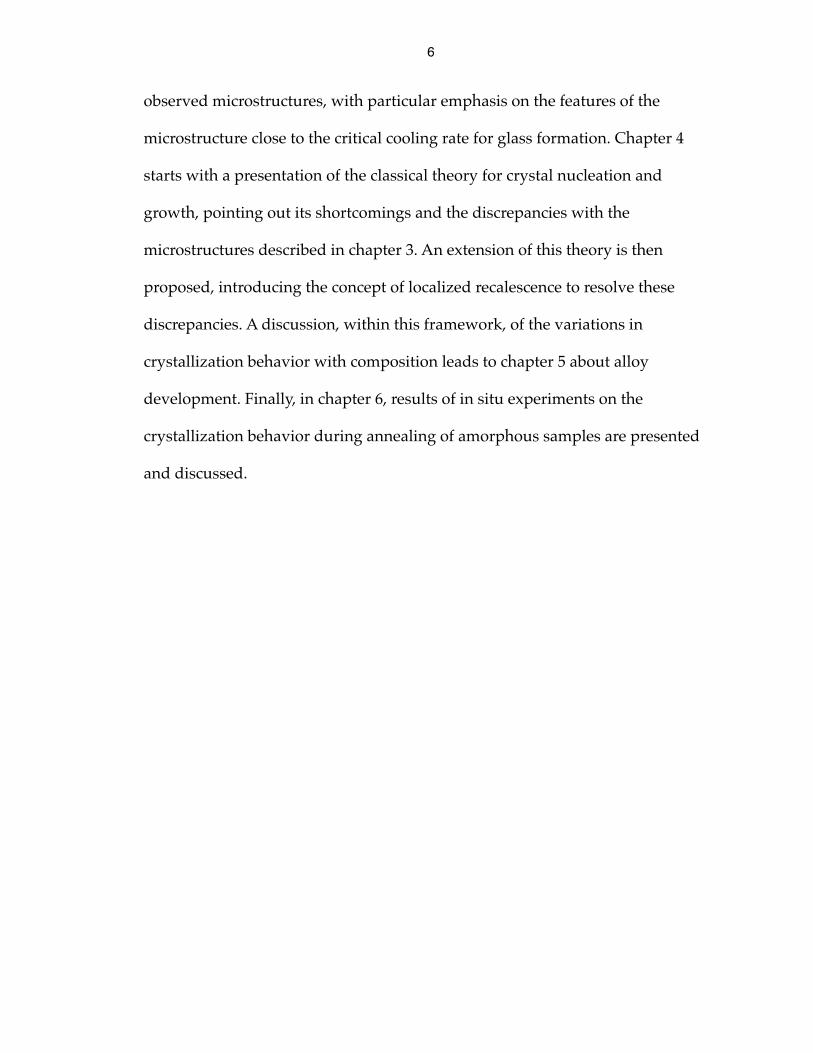
Figure 2.1: induction melting apparatus

The sample is molten on a water-cooled copper boat, which is enclosed in a fused

silica tube sealed off with vacuum fittings. The induction coil is wrapped around

the fused silica tube. Power is provided by a 15 kW Lepel LSS-15 radio frequency

generator. A vacuum pumping system is connected to the fittings on the fused

silica tube to evacuate the tube and fill it with an inert atmosphere, typically

titanium gettered ultra high purity argon. The fused silica tube with the copper

boat is supported on a carriage system, so that the boat can be moved freely inside

the induction coil.

10

Compositions

In order to study the composition dependence of the crystallization behavior in

the Vit101 alloy system, a series of alloys were made in which the composition

was systematically varied. For each of the alloys, the composition of Vit101 was

modified by decreasing the amount of one of the elements by 1 at.% compensated

by an increase in the amount of one of the other elements. This results in 12

compositions symmetrically located* around Vit101 in composition space, as

shown in Fig. 2.2.

* The compositions are located at the vertices of a cuboctahedron with the Vit101

composition at its center. This is also the geometry of the 12 nearest neighbors of an

atom in a face centered cubic lattice.

Figure 2.2: alloy compositions

Position in the three-dimensional Cu-Ni-Ti-Zr composition space, relative to

Vit101, of the 12 alloys studied in this work. The color code reinforces the depth

cues corresponding to the Cu-Ni axis.

Ti

ZrCu

Ni

11

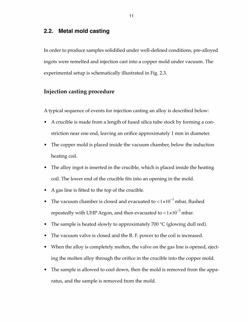
2.2. Metal mold casting

In order to produce samples solidified under well-defined conditions, pre-alloyed

ingots were remelted and injection cast into a copper mold under vacuum. The

experimental setup is schematically illustrated in Fig. 2.3.

Injection casting procedure

A typical sequence of events for injection casting an alloy is described below:

• A crucible is made from a length of fused silica tube stock by forming a con-

striction near one end, leaving an orifice approximately 1 mm in diameter.

• The copper mold is placed inside the vacuum chamber, below the induction

heating coil.

• The alloy ingot is inserted in the crucible, which is placed inside the heating

coil. The lower end of the crucible fits into an opening in the mold.

• A gas line is fitted to the top of the crucible.

• The vacuum chamber is closed and evacuated to < mbar, flushed

repeatedly with UHP Argon, and then evacuated to < mbar.

• The sample is heated slowly to approximately 700 °C (glowing dull red).

• The vacuum valve is closed and the R. F. power to the coil is increased.

• When the alloy is completely molten, the valve on the gas line is opened, eject-

ing the molten alloy through the orifice in the crucible into the copper mold.

• The sample is allowed to cool down, then the mold is removed from the appa-

ratus, and the sample is removed from the mold.

1 1–×10

1 3–×10

12

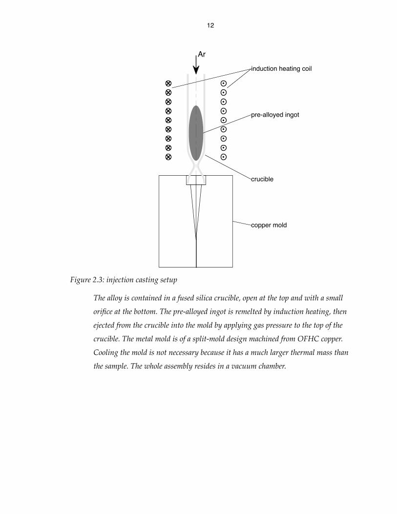
Figure 2.3: injection casting setup

The alloy is contained in a fused silica crucible, open at the top and with a small

orifice at the bottom. The pre-alloyed ingot is remelted by induction heating, then

ejected from the crucible into the mold by applying gas pressure to the top of the

crucible. The metal mold is of a split-mold design machined from OFHC copper.

Cooling the mold is not necessary because it has a much larger thermal mass than

the sample. The whole assembly resides in a vacuum chamber.

Ar

induction heating coil

pre-alloyed ingot

copper mold

crucible

13

Cooling rates in metal mold casting

The cooling rate obtained by metal mold casting depends primarily on the

geometry of the mold. Neglecting convection, i.e., assuming that a quiescent melt

of uniform temperature fills the mold instantly, the evolution of the temperature

profile in the mold is described by the Fourier heat flow equation:

, (2.1)

where T is temperature, t is time, is the heat capacity per unit volume, κ is the

thermal conductivity and is the thermal diffusivity. The boundary

conditions can be idealized* as a fixed temperature at the mold surface.

A formal solution to the Fourier equation is obtained by using the spectral

representation of the Laplacian† with these boundary conditions. The coefficient

of each of the terms in the spectral representation decays exponentially with a

time constant where is the eigenvalue of the Laplacian for that

term. The physical interpretation of is the inverse of a characteristic length scale

for the temperature variation.

* Since the thermal conductivity of the copper mold (400 W/m K) is much larger than

that of the melt (4 W/m K), and the mold is much more massive (>2 kg) than the

sample (a few grams), this is a reasonable approximation provided that the melt

remains in good thermal contact with the mold.

† The spectral representation of a linear operator amounts to a projection onto the

eigenfunctions of the operator. In one dimension, for example, the eigenfunctions of the

Laplacian are sine and cosine functions, so that the spectral representation is the

familiar Fourier series (See “Solutions to the Fourier heat flow equation” on page 75 for

applications).

t∂∂T 1

ρcP--------- κ T∇( )∇• α T∇2= =

ρcP

α κ ρcP⁄=

τ 1 αk2( )⁄= k2–

k

14

For long times the solution is dominated by the term with the longest time

constant, i.e., the term involving the eigenfunction for which the characteristic

length scale is the size of the sample. It leads to an asymptotic cooling rate

. This is consistent with the scaling law , where L is

the characteristic length scale for the problem, which can be deduced from

dimensional analysis of the Fourier heat flow equation and, as such, is more

generally valid.

Wedge-shaped samples

In order to evaluate the solidification microstructure as a function of cooling rate,

a mold was designed for casting wedge-shaped samples. A technical drawing

specifying the mold design is shown in Fig. 2.4. In a wedge geometry, the

thickness of the sample varies along its length*, resulting in a systematic variation

of the cooling rate. Near the tip of the wedge, the cooling rate profile depends

only on the opening angle of the wedge, so that results for wedges of different

sizes can be compared if all three dimensions are scaled uniformly.

For each of the compositions studied, one or more wedge-shaped samples were

cast. The as-cast samples were sectioned along their center line using a diamond

saw. One half of the sample was then polished for optical microscopy and SEM.

The other half was sectioned again, perpendicular to the center line into 1 mm

slices, for X-ray diffraction and TEM samples. This is illustrated in Fig. 2.5.

* A conical geometry could have been used as well, but the wedge-shaped mold is easier

to machine.

T T τ⁄ αTk2= = T αT L2⁄∝

15

Figure 2.4: drawing of wedge mold

The mold is of a split mold design, machined from OFHC copper bar stock. The

resulting wedge-shaped casting is 30 mm long, 6 mm wide, and the thickness

varies linearly from 0.2 mm at the tip to 6 mm at the end.

TOP ISOMETRIC

FRONT RIGHT

30

66

0.2

16

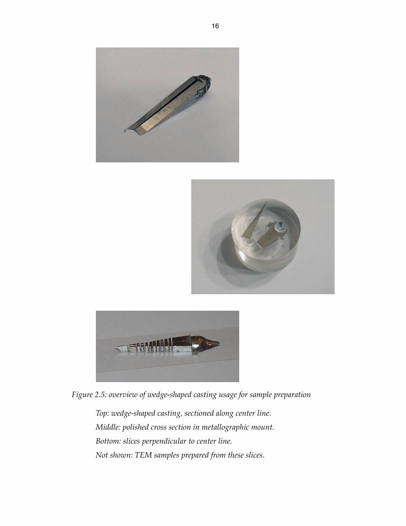
Figure 2.5: overview of wedge-shaped casting usage for sample preparation

Top: wedge-shaped casting, sectioned along center line.

Middle: polished cross section in metallographic mount.

Bottom: slices perpendicular to center line.

Not shown: TEM samples prepared from these slices.

17

2.3. Microstructure characterization

Metallography

The half of the wedge-shaped casting to be used for metallography was

embedded in a polyester mounting compound, Buehler castolite resin No.

20-8120-002 and hardener No. 20-8122-002. In order to fit the sample in the

mounting cup the sample was cut in half. Mounting these two halves in the same

mount had the added benefit of helping to keep the sample flat during polishing.

The resin was cured at 60 °C for 8 to 12 hours. The surface was then ground flat

using a succession of SiC grinding papers and polished.

Polishing with diamond paste or alumina slurry resulted in a poor polish with

severe pitting of the sample surface. Such pitting can be the result of “pullout,”

which occurs when polishing with an abrasive of the same size as the

microstructure of the material to be polished. With these samples this occurred at

all abrasive sizes, presumably because the wide range of cooling rates in the

sample results in a wide range of microstructure length scales. Pitting was

eliminated by using diamond lapping film instead of a slurry for polishing.

The polished samples were examined on an inverted reflected light microscope

using polarized light. Images were acquired in digital form using a TV camera

connected to a frame grabber. When the resolution or the field of view of the

camera was insufficient, overlapping images were acquired and pasted together

using image manipulation software.

18

Scanning electron microprobe (SEM/microprobe)

Some of the samples used for optical microscopy were subsequently

carbon-coated and examined in a JEOL model JXA-733 microprobe equipped

with 5 wavelength-dispersive spectrometers. Images were acquired using the

backscattered electron detector, with the goal of minimizing any topographical

contrast in the image and obtaining an image where contrast is due mainly to

variations in composition. Composition measurements were performed with the

spectrometers, using the pure metals as standards and the CITZAF correction

package [18].

X-ray diffraction

Diffraction patterns were obtained from sections perpendicular to the long axis of

the wedge-shaped samples at various thicknesses. The experiments were carried

out using Co K-α radiation and an inel CPS-120 curved position sensitive

detector. The samples were supported on a glass slide for the measurement. The

channel numbers of the output from the inel detector were calibrated as 2θ angles

using a polycrystalline silicon diffraction standard.

Transmission electron microscopy (TEM)

A few samples were further investigated by transmission electron microscopy.

The microscope used is a Philips model EM430, equipped with a LaB6 filament.

19

TEM samples were prepared from the 1 mm slices by ultramicrotomy. Before it is

mounted in the microtome, the sample is filed away around the region of interest

until only a tip at the region of interest remains. Using the microtome, TEM

samples are then sliced from this tip with a diamond knife edge, collecting the

samples on the surface of a small water reservoir behind the knife edge. The TEM

samples are picked up from the water surface with a holey carbon grid which fits

inside the microscope sample holder.

The TEM images shown are dark field electron micrographs obtained with a

70 µm objective aperture selecting intensity from the first diffraction ring. Since

the interatomic spacing in the glass is comparable to the interatomic spacing in

crystalline phases, any diffraction spots from nanocrystals overlap the diffuse

diffraction ring from the amorphous phase. As a result, these dark field conditions

highlight crystallites in the corresponding range of orientations, as well as (but

more brightly than) the amorphous phase.

2.4. Annealing

Low-temperature crystallization studies were performed by annealing

amorphous samples at temperatures slightly above the glass transition. For this

purpose, pre-alloyed Vit101 samples were cast into 1 mm thick strips, 10 mm

wide and 25 mm long, which were then sectioned into two 10 mm squares using a

diamond saw. These squares were wrapped in tantalum foil, sealed in a fused

20

quartz tube under vacuum of or lower, and annealed in a resistively

heated tube furnace at various temperatures.

Differential scanning calorimetry (DSC)

A Perkin-Elmer DSC-7 differential scanning calorimeter was used to study the

thermal behavior of such pre-annealed Vit101 samples. The DSC scans were taken

with a heating rate of 0.333 K/s.

Small angle X-ray scattering (SAXS)

In situ SAXS experiments were performed at the Basic Energy Science

Synchrotron Radiation Center (BESSRC) at the Advanced Photon Source (APS),

Argonne National Laboratory. SAXS requires X-ray transparent samples, so splat

quenched foils, between 30 and 50 µm thick, were prepared. The energy of the

photons was 13.5 keV, corresponding approximately to 1 Å wavelength. The raw

data from the two-dimensional position sensitive detector was averaged over the

azimuthal angle to obtain the radial average scattered intensity which was

analyzed.

5 6–×10 mbar

21

3. Microstructure

3.1. Metallography

Polished cross sections of wedge-shaped castings of different alloys were

observed by optical microscopy. Contrast was obtained by using polarized light.

Composite images of typical cross sections are shown in Fig. 3.1 and Fig. 3.2.

Similar microstructures are observed for each of the alloy compositions studied.

The positions in the sample where these microstructures occur roughly scale with

a critical thickness which depends on composition.

Near the tip of the wedge and at the surface, where the cooling rate was highest,

the sample is completely amorphous as determined by X-ray diffraction and TEM

analysis. Near the base of the wedge, where the cooling rate was lowest, the

sample is nearly fully crystallized. In the region between the crystallized part and

the fully amorphous part of the sample, spherical features are observed in the

optical micrograph, with diameters ranging from <10 µm to 300 µm. Similar

features have also been observed in other bulk glass forming alloys cooled from

the melt, including Zr41.2Ti13.8Cu12.5Ni10Be22.5 [19] and

Zr58.5Nb2.8Cu15.6Ni12.8Al10.3 [20], but they have received little attention. As

illustrated in Fig. 3.3, the size and number density of these spheres increase

continuously from the amorphous part of the sample, where there are none, to the

fully crystallized part, where the spheres coalesce leaving no space in between.

22

Figure 3.1: optical micrograph of Cu48Ni8Ti34Zr10 wedge

Cross section from the center of an as-cast wedge-shaped sample, showing

spherical features increasing in size and number density with decreasing cooling

rate. The large dark areas in the center are cavities in the sample.

23

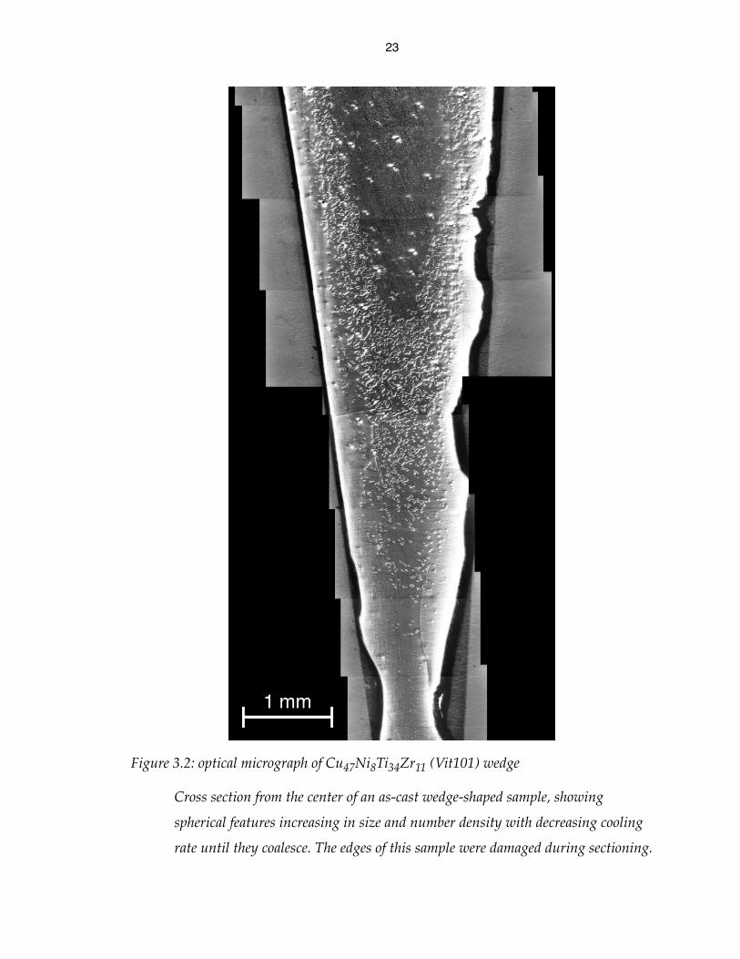
Figure 3.2: optical micrograph of Cu47Ni8Ti34Zr11 (Vit101) wedge

Cross section from the center of an as-cast wedge-shaped sample, showing

spherical features increasing in size and number density with decreasing cooling

rate until they coalesce. The edges of this sample were damaged during sectioning.

24

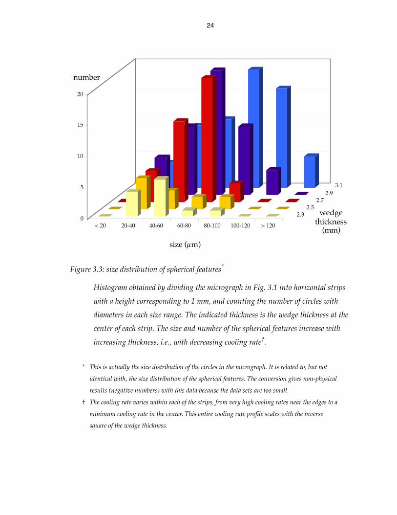
Figure 3.3: size distribution of spherical features*

Histogram obtained by dividing the micrograph in Fig. 3.1 into horizontal strips

with a height corresponding to 1 mm, and counting the number of circles with

diameters in each size range. The indicated thickness is the wedge thickness at the

center of each strip. The size and number of the spherical features increase with

increasing thickness, i.e., with decreasing cooling rate†.

* This is actually the size distribution of the circles in the micrograph. It is related to, but not

identical with, the size distribution of the spherical features. The conversion gives non-physical

results (negative numbers) with this data because the data sets are too small.

† The cooling rate varies within each of the strips, from very high cooling rates near the edges to a

minimum cooling rate in the center. This entire cooling rate profile scales with the inverse

square of the wedge thickness.

0

5

10

15

20

< 20 20-40 40-60 60-80 80-100 100-120 > 120

2.32.5

2.72.9

3.1

size (µm)

number

wedge thickness

(mm)

25

In addition to these spherical features, there are also some dendrites visible in

Fig. 3.1. The dendrites seem not to have influenced the crystallization of the

surrounding material. Dendrites are not observed in some of the other samples

with different compositions, while the spherical features were observed in every

sample studied. Assuming a definition of glass forming ability that tolerates the

presence of a small volume fraction of crystals, it appears that the glass forming

ability in the Vit101 alloy system is limited by the formation of the spherical

features, and not by the formation of these dendritic crystals.

The thickness where these spherical features occupy a given volume fraction* of

the sample can then be taken to be a measure of the critical casting thickness for

glass formation. The chosen threshold value is of course somewhat arbitrary;

using a different threshold value —or a different criterion for glass formation

altogether— would result in a slightly different value for the critical casting

thickness. This does not hinder comparisons of the critical thickness between

different samples, provided that the difference from one criterion to another is

similar for each of the samples.

The wedge thickness where the spherical features occupy roughly 5% in the

optical micrograph was evaluated for a series of alloys in which the composition

was systematically varied. The results are listed in Table 3.1, and represented

graphically as a “bubble chart” in Fig. 3.4. No clear trends emerge from this data.

* If there is no preferred orientation, the fractional area occupied by features in a cross

section is equal to their volume fraction.

26

Surprisingly, the central composition (Vit101) is the worst glass former*. One

would have expected a local maximum in the critical casting thickness near a

good glass forming composition, not a local minimum! There is no immediately

obvious direction in composition space which gives a larger improvement in glass

Table 3.1: variation of critical casting thickness with composition

Composition critical casting thickness(mm)

Cu47Ni8Ti34Zr11 (Vit101) 1.1

Cu46Ni9Ti34Zr11 2.5

Cu46Ni8Ti35Zr11 4.0

Cu46Ni8Ti34Zr12 3.5

Cu48Ni7Ti34Zr11 2.5

Cu47Ni7Ti35Zr11 1.5

Cu47Ni7Ti34Zr12 3.2

Cu48Ni8Ti33Zr11 1.8

Cu47Ni9Ti33Zr11 3.1

Cu47Ni8Ti33Zr12 3.5

Cu48Ni8Ti34Zr10 2.6

Cu47Ni9Ti34Zr10 5.5

Cu47Ni8Ti35Zr10 3.5

* This is not due to experimental error. Several samples with the Vit101 composition

were cast successfully, allowing the variability of the critical casting thickness to be

estimated at ±20% for successful castings. Unsuccessful castings —e.g., where the

crucible broke during casting— resulted in similar or lower critical casting thickness

than successful castings.

27

forming ability than other directions. More compositions would need to be

studied in order to form a more complete picture of the composition dependence

of the glass forming ability in this alloy system.

Figure 3.4: variation of critical casting thickness with composition

Projection of 12 compositions, located on the vertices of a cuboctahedron centered

on Vit101 in the three-dimensional Cu-Ni-Ti-Zr composition space. For each of the

compositions, a circle is drawn whose size is proportional to the critical casting

thickness of that composition (cfr. Table 3.1). The color code reinforces the depth

cues corresponding to the Cu-Ni axis.

Ti

ZrCu

Ni

28

3.2. SEM

Some of the samples used for optical microscopy were also examined in an SEM.

Fig. 3.5 shows some of the spherical features in a backscattered electron image. To

make the spherical features visible, the gain control was set to the maximum.

Even then the spherical features are barely visible. No internal structure is

discernible inside the sphere. Since the backscattered electron image is sensitive to

composition changes*, this indicates that to within the resolution of the

Figure 3.5: SEM micrograph of Cu46Ni8Ti35Zr11 wedge

The arrow points to one of the spherical features.

* The backscattered electron intensity is related to the average square of the atomic

number of the sample. As such, the backscattered electron image for Vit101 and related

alloys corresponds to a map of variations in the Zr content of the alloy.

29

instrument, the composition of the spheres is spatially uniform. The microprobe

capability of the instrument was also used to look for any composition difference

between the spheres and the surrounding material. Again, the composition was

found to be uniform.

For comparison, Fig. 3.6 shows a sample with a smaller critical casting thickness,

near the base of the wedge, where it is nearly fully crystallized. Here the

microstructure is readily apparent in the backscattered electron image, without

increasing the gain.

Figure 3.6: SEM micrograph of crystallized Cu48Ni8Ti33Zr11 alloy

30

3.3. X-ray diffraction

Diffraction patterns obtained from sections perpendicular to the long axis of the

wedge-shaped samples at various thicknesses are shown in Fig. 3.7. These slices

contain material that was cooled at a variety of cooling rates, ranging from very

high cooling rates at the sample surface to a minimum cooling rate which

depends on the thickness of the wedge at that point.

The diffraction pattern from the tip of the sample is a typical diffraction pattern

for an amorphous material [21], showing two broad maxima. The diffraction

pattern from the slice at 3 mm thickness is indistinguishable from the first. From 3

to 4 mm thickness the broad maximum from the amorphous diffraction pattern

gradually becomes sharper. Comparing this change in shape with the patterns

from >4 mm, it can be attributed to an emerging crystalline pattern superimposed

on the amorphous background*.

The peaks in the crystalline pattern are significantly broadened, which makes

them harder to detect against the amorphous background. This peak broadening

could be due to, e.g., an inhomogeneous strain distribution in the crystals or to

the effect of small crystallite size [22].

When the diffraction patterns are compared with the micrographs from the same

thickness, the spherical features are found to appear in the optical and SEM

* The amorphous background comes from the edges of the slice, which experienced a

higher cooling rate than the center.

31

Figure 3.7: variation of X-ray diffraction pattern with thickness

X-ray diffraction patterns from a series of slices of a Cu48Ni8Ti34Zr10 wedge. The

background signal obtained with only the glass slide used for supporting the

samples is also displayed. The indicated thickness is the thickness of the wedge

where the slice was taken.

inte

nsit

y

120°100806040202θ

glass slide

wedge tip

3 mm

3.3 mm

3.9 mm4.1 mm

4.3 mm

4.5 mm

32

micrographs at smaller thicknesses than the crystalline peaks in the diffraction

pattern. The crystalline peaks are clearly distinguishable only when the spherical

features are so large and closely spaced that they merge together. The size of the

spherical features is also far too large to account for any significant peak

broadening under the assumption that the crystallite size is the size of the

spheres. In combination with the lack of any composition variation inside the

spheres or between the spheres and the surrounding material —while crystals are

expected to form only at compositions different from the nominal composition of

the alloy— this makes it unlikely that the spherical features are individual

crystals.

3.4. TEM

To further characterize the microstructure in the as-cast alloys with higher spatial

resolution, a few alloys were studied by transmission electron microscopy. The

TEM samples were prepared by ultramicrotomy. There are some artefacts, such as

streaks and holes, visible in the micrographs, which are a consequence of this

preparation technique.

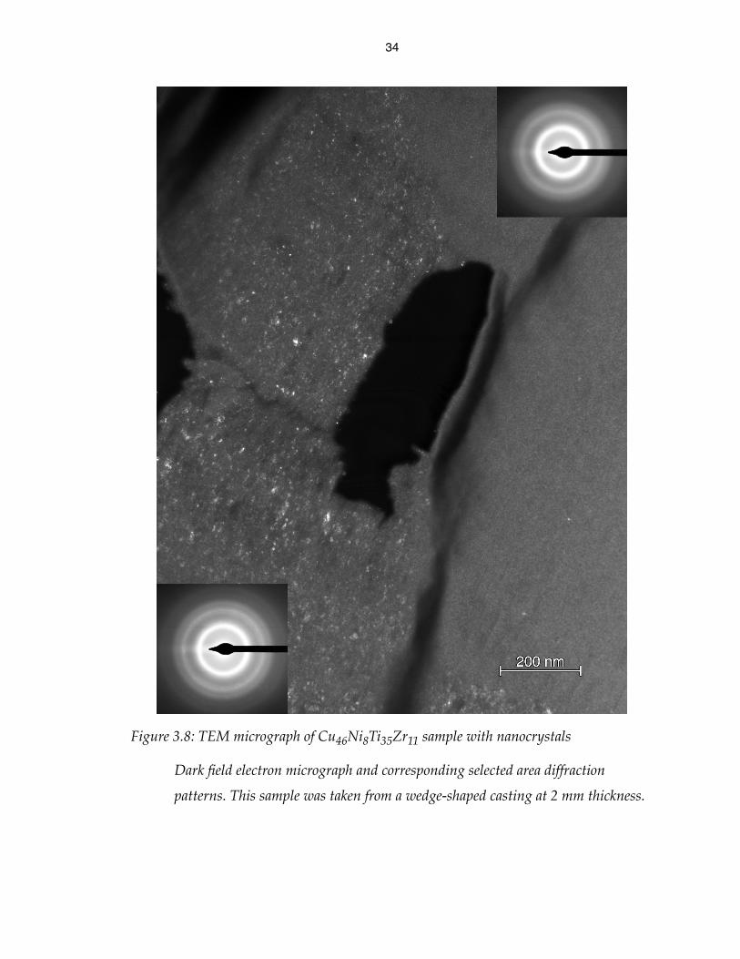
The sample for the TEM micrograph in Fig. 3.8 was taken from a part of the

wedge where spherical features appear in the optical micrographs. The sample

preparation started from the unpolished half of the sample. Since the features can

not be distinguished on an unpolished surface, the location where this sample

was taken, relative to the features in the optical micrograph, is unknown. The

33

sample could have come from inside one of the spheres, from the surrounding

material, or from the interface between them.

Figure 3.8 shows a TEM dark field micrograph, with two very different

microstructures separated by a sharp interface. Selected area diffraction (SAD)

patterns corresponding to each of the regions are also shown as insets.

The region in the lower left of the micrograph is characterized by a large density

of distinguishable nanocrystals. The corresponding diffraction pattern also

indicates a nanocrystalline microstructure; compared to that of a fully amorphous

material, the first diffraction ring is sharper, the second diffuse ring has split into

several rings in which individual diffraction spots start to appear, and a third ring

has become visible.

The region in the upper right of the micrograph is comparatively featureless. Few,

if any, nanocrystals are highlighted in that part of the sample under these dark

field conditions. The diffraction pattern resembles that of an amorphous sample

more closely than the one in the lower left, but still shows some of the signs of

short range order mentioned above. The microstructure in the lower left of the

micrograph is certainly coarser, with a much higher density of nanocrystals, so

the distribution of nanocrystals can be said to be spatially localized.

34

Figure 3.8: TEM micrograph of Cu46Ni8Ti35Zr11 sample with nanocrystals

Dark field electron micrograph and corresponding selected area diffraction

patterns. This sample was taken from a wedge-shaped casting at 2 mm thickness.

35

3.5. Conclusions

The TEM micrograph shows that the distribution of nanocrystals in these samples

is spatially localized. The other results can be explained as well, if the spheres in

Fig. 3.1 and Fig. 3.2 correspond to the regions with a high density of nanocrystals.

The contrast in the optical micrographs could be due to a difference in optical

properties or to different mechanical properties leading to different polishing

behavior resulting in topographic contrast. In agreement with the observations by

SEM, there would be no concentration changes on length scales large compared to

the size of the nanocrystals. And the size effect would broaden X-ray diffraction

peaks to the point where they are hardly detectable when superimposed on the

pattern from the surrounding amorphous material. Thus, the ensemble of

experimental results presented in this chapter suggests that crystallization near

the critical cooling rate is locally enhanced in spherical regions which form a large

number of nanocrystals.

36

4. Crystallization Kinetics

In the proposed microstructure, spherical features contain a much higher number

density of crystals than the surrounding regions, even though they have the same

composition and seemingly experienced the same temperature history. This is not

the crystallization behavior expected on the basis of established theories. It is

postulated that these features did not in fact experience the same temperature

history as the surrounding regions, but mark the site of localized recalescence

events.

This claim is supported by the linear stability analysis of a set of differential

equations describing the heat flow problem coupled with crystal nucleation and

growth kinetics. The derivation, under “Spatially localized nucleation” on

page 47, relies only on the inclusion of the heat of crystallization in the heat flow

problem and some general characteristics of the temperature dependence of the

nucleation and growth rates. The latter are adequately described by classical

nucleation and growth theories, and are not fundamentally changed in more

sophisticated descriptions of crystallization behavior.

37

4.1. Classical nucleation and growth kinetics

Classical nucleation theory

In classical nucleation theory [23-26], it is postulated that the free energy of a

nucleus consists of a negative term proportional to the volume of the nucleus and

a positive term proportional to the interfacial area between the nucleus and the

liquid: for a spherical nucleus of radius r. As a result,

growth only lowers the free energy of a nucleus once it has surpassed the critical

size , corresponding to a free energy barrier for

nucleation. With some loss of generality, the parameters and may be

equated with the bulk values of the free energy difference per unit volume

between solid and liquid and the interfacial tension between solid and liquid,

respectively.

Heterogeneous nucleation can occur at the interface between the liquid and

another phase, if the crystal wets the other phase. A critical nucleus can then be

formed at the interface between the liquid and the other phase with a smaller

number of atoms than in the bulk liquid. This results in a reduction of the free

energy barrier for nucleation by a factor , where

is the wetting angle.

G∆ f43---πr3 g∆ f 4πr2σsf+=

r‡ 2σsf ∆gf⁄–= G∆ ‡ 16π

3---------

σsf3

g∆ f2

---------=

g∆ f σsf

f θ( ) 2 θcos+( ) 1 θcos–( )2( ) 4⁄=

θ

38

The free energy of a critical nucleus can be regarded as the activation energy

for nucleation in an Arrhenius equation* for the steady-state nucleation rate :

. (4.1)

The kinetic prefactor A takes into account the number of potential sites for

heterogeneous or homogeneous nucleation, as well as the temperature

dependence of the mobility in the liquid.

The temperature dependence of the nucleation rate results from thermodynamic

as well as kinetic factors. Above the liquidus temperature, the liquid is

thermodynamically stable, so no crystals can form and the nucleation rate is zero.

As the liquid is undercooled below the liquidus temperature, the thermodynamic

driving force for crystallization increases, i.e., becomes more negative. This

reduces the nucleation barrier , so that the nucleation rate increases. Close to

the glass transition, however, the temperature dependence of the nucleation rate

is dominated by the temperature dependence of the kinetic prefactor; the

nucleation rate decreases again as the mobility in the liquid decreases rapidly

with decreasing temperature.

In a first approximation, the thermodynamic driving force varies linearly with the

undercooling below the liquidus temperature: . The

proportionality constant is the entropy of fusion , where is

* This does not imply that the temperature dependence of the nucleation rate follows an

Arrhenius law. The activation energy and the prefactor in this expression are strongly

temperature dependent.

G∆ ‡

Iν

Iν AG∆ ‡

–kBT

-------------

exp=

∆gf

G∆ ‡

∆gf ∆Sf T Tliq–( )=

∆Sf ∆Hx Tliq⁄= ∆Hx

39

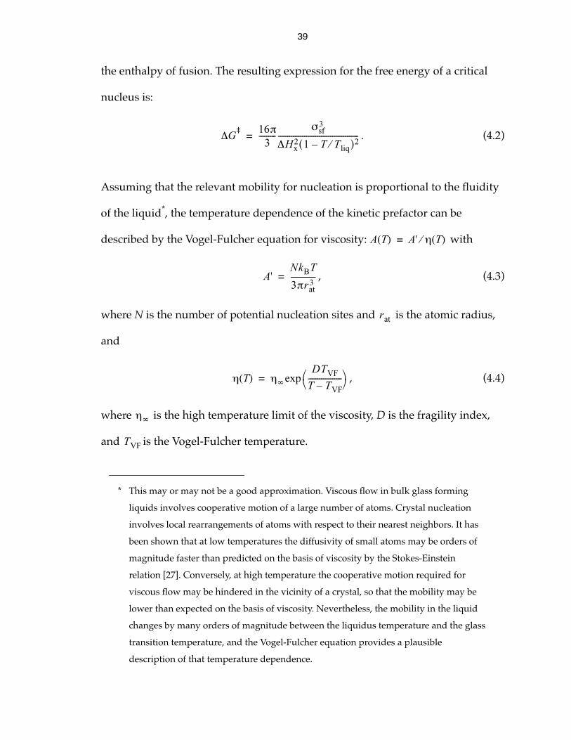
the enthalpy of fusion. The resulting expression for the free energy of a critical

nucleus is:

. (4.2)

Assuming that the relevant mobility for nucleation is proportional to the fluidity

of the liquid*, the temperature dependence of the kinetic prefactor can be

described by the Vogel-Fulcher equation for viscosity: with

, (4.3)

where N is the number of potential nucleation sites and is the atomic radius,

and

, (4.4)

where is the high temperature limit of the viscosity, D is the fragility index,

and is the Vogel-Fulcher temperature.

* This may or may not be a good approximation. Viscous flow in bulk glass forming

liquids involves cooperative motion of a large number of atoms. Crystal nucleation

involves local rearrangements of atoms with respect to their nearest neighbors. It has

been shown that at low temperatures the diffusivity of small atoms may be orders of

magnitude faster than predicted on the basis of viscosity by the Stokes-Einstein

relation [27]. Conversely, at high temperature the cooperative motion required for

viscous flow may be hindered in the vicinity of a crystal, so that the mobility may be

lower than expected on the basis of viscosity. Nevertheless, the mobility in the liquid

changes by many orders of magnitude between the liquidus temperature and the glass

transition temperature, and the Vogel-Fulcher equation provides a plausible

description of that temperature dependence.

G∆ ‡ 16π3

---------σsf

3

∆Hx2 1 T Tliq⁄–( )2

-------------------------------------------=

A T( ) A' η T( )⁄=

A'NkBT

3πrat3

-------------=

rat

η T( ) η∞

DTVF

T TVF–------------------

exp=

η∞

TVF

40

Substituting Eq. 4.2 and Eq. 4.4 into Eq. 4.1, the following expression for the

steady state nucleation rate is obtained:

. (4.5)

The contributions of the thermodynamic driving force and of the kinetic prefactor

to the temperature dependence of the nucleation rate are illustrated in Fig. 4.1.

Figure 4.1: temperature dependence of nucleation rate

The dotted line illustrates the influence of the kinetic prefactor by using the heat of

fusion instead of the temperature dependent thermodynamic driving force in the

activation energy. The dashed line similarly illustrates the effect of the

thermodynamic driving force by keeping the viscosity constant at its high

temperature limit.

IνA'η∞-------

DTVF

T TVF–------------------–

exp16π

3--------- 1

kBT---------

σsf3

∆Hx2 1 T Tliq⁄–( )2

-------------------------------------------–

exp=

1035

1030

1025

1020

1015

1010

105

100

nucl

ei/

m^

3/s

1100K1000900800700600500

41

Validity of classical nucleation theory

Classical nucleation theory ignores several important aspects of nucleation in

bulk metallic glass forming liquids. For example, it is implicitly assumed that

crystallization is polymorphic, which is certainly not the case in Vit101. It is also

questionable whether a description of the steady state nucleation rate is

applicable to the instantaneous nucleation rate during continuous cooling. At

best, classical nucleation theory provides a simplistic description of the complex

process of nucleation in bulk metallic glass forming liquids.

It should be noted, however, that the nucleation rate varies over many orders of

magnitude between the liquidus temperature and the glass transition

temperature, and classical nucleation theory does capture the essential features of

this temperature dependence. As a liquid is cooled from the melt, the nucleation

rate initially increases with increased undercooling below the liquidus

temperature and then decreases again as the mobility in the liquid decreases. This

is in agreement with experimentally determined TTT-diagrams (See

“TTT-diagrams” on page 44).

Using a more sophisticated description of the nucleation process, e.g., taking into

account transient effects or partitioning, is unjustified unless it results in

improved agreement with experiments. The calculated classical nucleation rate

depends sensitively on parameters like interfacial tension*, which are not

* A reduction of the interfacial tension from 150 mJ to 140 mJ increases the calculated

maximum nucleation rate in Vit101 by a factor of 200.

42

precisely known. As a result, there is a large uncertainty inherent in calculated

nucleation rates, and the interfacial tension is usually treated as a fitting

parameter. If the more sophisticated description introduces new parameters with

similar uncertainty, the additional fit parameters may improve quantitative

agreement with experimental data, but in a physically meaningless way.

Crystal growth rate

Using transition state rate theory, the crystal growth velocity u can be expressed

as the rate at which atoms from the liquid impinge on the crystal liquid interface,

multiplied by a thermodynamic “sticking coefficient”:

. (4.6)

Similarly to the nucleation rate, the temperature dependence of the crystal growth

rate is explained by the competing effects of increasing thermodynamic driving

force and decreasing mobility as the liquid is cooled below the liquidus

temperature. Contrary to nucleation, crystal growth does not require significant

undercooling below the liquidus temperature; the maximum growth rate occurs

at higher temperature than the maximum nucleation rate.

As was the case for the classical nucleation rate, this expression is strictly valid

only for polymorphic crystallization. If the crystallization is non-polymorphic,

partitioning will cause the composition of the liquid at the crystal liquid interface

to differ from that of the bulk liquid. This normally* has the effect of lowering the

crystal growth rate. As a result, the crystal growth rate becomes coupled to a

ukη--- 1

g∆ f–

kBT-----------

exp– =

43

diffusion problem. Diffusion leads to a growth law where the crystal

size is proportional to the square root of time rather than where it is

directly proportional to time. Thus, sooner or later, the interface always overtakes

the composition gradient. As the crystal grows and the composition difference

between the liquid at the interface and the bulk liquid builds up, mass transport

then becomes the dominating factor in the crystal growth rate.

Partitioning, by reducing the growth rate at the crystal liquid interface, also favors

dendritic growth [28]. In the case of dendritic growth, the relevant length scale for

the mass transport is not the size of the crystal, but the radius of curvature at the

dendrite tip, resulting in a scaling law , where the size of the

dendrite is again directly proportional to time. This would indicate that smaller

dendrites always grow faster, but the increased interfacial area of smaller

dendrites decreases the thermodynamic driving force for the crystallization. The

microstructure is dominated by the dendrite arm size whose balance of mass

transport and interfacial area results in the highest growth rate.

In summary, the simple picture of crystal growth limited by the rate interface

attachment is complicated by mass transport effects in the case of

non-polymorphic crystallization. This has ramifications for the crystal growth

* Partitioning decreases the driving force for crystallization, unless the curvature of the

Gibbs free energy with respect to composition is negative. However, when this is the

case, the nucleation and growth rates are likely to be influenced by spinodal

decomposition, so that the classical nucleation and growth rates are no longer

applicable.

r Ddifft∝

r ut∝

r Ddifft rtip⁄∝

44

rate and for the resulting microstructure, but in each case the temperature

dependence of the crystal growth rate is determined by the competing effects of

thermodynamic driving force and mobility.

TTT-diagrams

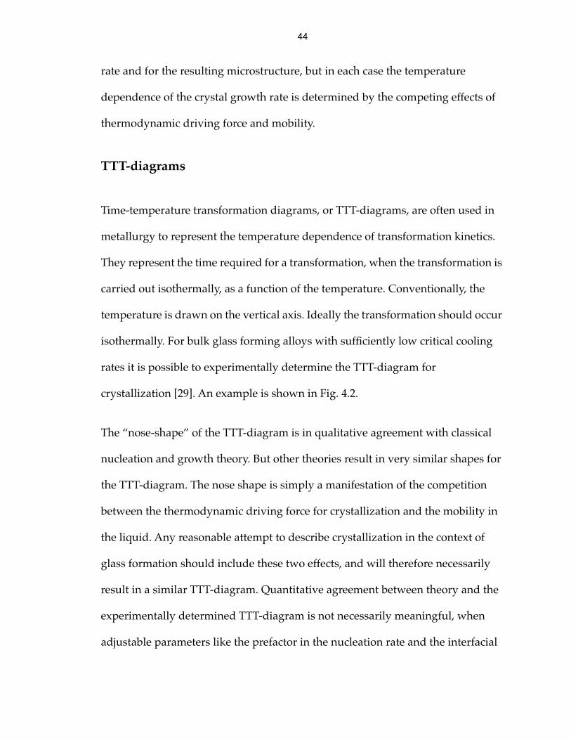
Time-temperature transformation diagrams, or TTT-diagrams, are often used in

metallurgy to represent the temperature dependence of transformation kinetics.

They represent the time required for a transformation, when the transformation is

carried out isothermally, as a function of the temperature. Conventionally, the

temperature is drawn on the vertical axis. Ideally the transformation should occur

isothermally. For bulk glass forming alloys with sufficiently low critical cooling

rates it is possible to experimentally determine the TTT-diagram for

crystallization [29]. An example is shown in Fig. 4.2.

The “nose-shape” of the TTT-diagram is in qualitative agreement with classical

nucleation and growth theory. But other theories result in very similar shapes for

the TTT-diagram. The nose shape is simply a manifestation of the competition

between the thermodynamic driving force for crystallization and the mobility in

the liquid. Any reasonable attempt to describe crystallization in the context of

glass formation should include these two effects, and will therefore necessarily

result in a similar TTT-diagram. Quantitative agreement between theory and the

experimentally determined TTT-diagram is not necessarily meaningful, when

adjustable parameters like the prefactor in the nucleation rate and the interfacial

45

tension can change the results by several orders of magnitude. The TTT-diagram

is a useful characterization of the crystallization behavior for practical purposes,

but it is not a good test to distinguish between various theoretical models.

Microstructure

A theoretical model of crystallization behavior should be judged not only on the

accuracy with which it predicts crystallization kinetics, but also on its ability to

explain the observed microstructures. The solidification microstructures of most

Figure 4.2: experimentally determined TTT-diagram

Time to onset of crystallization in graphite crucibles during isothermal

experiments after cooling from the melt, vs. temperature of the isothermal segment,

for Zr41.2Ti13.8Cu12.5Ni10Be22.5 (after Ref. [27]).

1000K

900

800

700

600

500

400

tem

pera

ture

10 s 100 s 1ks 10kstime

Tliq

Tg

46

metals and alloys can be interpreted in terms of classical nucleation and growth

theory, if heterogeneous nucleation and segregation effects due to partitioning are

included [30]. The temperature dependence of the mobility is insignificant in

most alloys, but when it is included glass formation can also be explained. More

specific mechanisms have been put forward to explain nanocrystalline

microstructures in glass forming alloys, including quenched-in nuclei [31], phase

separation prior to crystallization [32-34], and linked fluxes of interface

attachment and diffusion [35].

However, the most striking aspect of the microstructure described in chapter 3 is

that the spherical features contain a much higher number density of nanocrystals

than the surrounding regions. Neither classical nucleation theory, nor any of the

more specific mechanisms cited above, can explain such an inhomogeneous

distribution of nuclei. In these theories, nucleation is considered to occur either at

a heterogeneous nucleation site or randomly by a statistical fluctuation. To

explain spatial localization of the nucleation rate, a feedback mechanism must be

included to increase the likelihood of forming a nucleus in the vicinity of a

previously nucleated crystal. The heat of crystallization released by a growing

crystal can give rise to such a feedback mechanism. If the nucleation rate increases

with temperature, then recalescence causes more crystals to form.

47

4.2. Spatially localized nucleation

Recalescence usually has the effect of creating fewer crystals: the heat release

associated with crystal growth raises the temperature of the surrounding liquid,

decreasing the nucleation rate. But in deeply undercooled liquids, i.e., on the

“lower” branch of the TTT-diagram, the temperature dependence of the mobility

in the liquid overshadows the temperature dependence arising from the free

energy barrier for nucleation, so that the nucleation rate increases with increasing

temperature. This sign change in the temperature dependence of the nucleation

rate changes the nature of the recalescence instability.

Differential equations for nucleation and growth

To include the effect of the heat of crystallization, which is responsible for

recalescence, in the heat flow equation, a heat release term proportional to the

volume growth rate of the crystals is added in Eq. 4.7.a. This term couples

the crystallization behavior, described by nucleation in Eq. 4.7.b and growth in

Eq. 4.7.c, to the heat flow problem.

(4.7.a)

(4.7.b)

(4.7.c)

X∂ t∂⁄

t∂∂T α T∇2

∆Hx

cp----------

t∂∂X

+=

t∂∂N Iν T( )=

t∂∂X Vx

˙⟨ ⟩ T( )N=

48

, and are temperature, number density of crystals and volume fraction

crystallized, respectively. These variables are dependent on time and spatial

position. The parameters thermal diffusivity , heat of crystallization per unit

volume , and heat capacity are roughly constant, while the nucleation

rate is temperature dependent. The details of crystal growth kinetics are

lumped together in the average volume growth rate of the crystals, which

depends on the size distribution of the crystals as well as temperature.

Linear stability analysis

By linearizing these equations around a solution at an arbitrary point in

time , and using the spectral representation of the Laplacian*, a set of linear

ordinary differential equations with constant coefficients is obtained for each of

the terms in the spectral representation:

(4.8.a)

(4.8.b)

(4.8.c)

* The spectral representation of a linear operator amounts to a projection onto the

eigenfunctions of the operator. See “Solutions to the Fourier heat flow equation” on

page 75.

T N X

α

∆Hx cp

Iν

Vx˙⟨ ⟩

T0

N0

X0, ,

t0

t∂

∂Ti1

αki2Ti

1–

∆Hx

cp----------

t∂

∂Xi1

+=

t∂

∂Ni1

Iν' T0( )Ti

1=

t∂

∂Xi1

Vx˙⟨ ⟩ ' T

0( )Ti1Ni

0Vx˙⟨ ⟩ T

0( )Ni1

+=

49

and are the temperature derivatives, evaluated at , of the

nucleation and growth rates and , respectively. The superscript 1

refers to the deviation from the original solution with superscript 0. The subscript

i refers to the ith term in the spectral representation of the Laplacian, with

eigenvalue . In the case of rectangular boundary conditions for example, the

eigenfunctions of the Laplacian are the terms in a Fourier series, e.g., for

temperature , indexed by

three wavenumbers , with .

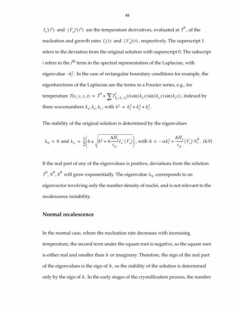
The stability of the original solution is determined by the eigenvalues

and , with . (4.9)

If the real part of any of the eigenvalues is positive, deviations from the solution

will grow exponentially. The eigenvalue corresponds to an

eigenvector involving only the number density of nuclei, and is not relevant to the

recalescence instability.

Normal recalescence

In the normal case, where the nucleation rate decreases with increasing

temperature, the second term under the square root is negative, so the square root

is either real and smaller than or imaginary. Therefore, the sign of the real part

of the eigenvalues is the sign of , so the stability of the solution is determined

only by the sign of . In the early stages of the crystallization process, the number

Iν' T0( ) Vx

˙⟨ ⟩ ' T0( ) T

0

Iv T( ) Vx˙⟨ ⟩ T( )

ki2–

T x y z t, , ,( ) T0

Tkx ky kz, ,1

t( ) kxx( )sin kyx( )sin kzx( )sin∑+=

kx ky kz, , k2 kx2 ky

2 kz2+ +=

λ0 0= λ±12--- δ δ2 4

∆Hx

cp----------Iν' Vx

˙⟨ ⟩+±

= δ αki2–

∆Hx

cp---------- Vx

˙⟨ ⟩ 'Ni0

+=

T0

N0

X0, , λ0

δ

δ

δ

50

density of nuclei is small, so is dominated by the thermal conductivity term

in Eq. 4.9, which is always negative. As the number of crystals increases, the

heat release term contributes more to , eventually making positive if the

growth rate increases with temperature. The first mode in the series expansion

becomes unstable when , where is the thickness of the

sample. This is the well-known recalescence phenomenon: the liquid is

undercooled until sufficient nuclei are formed, at which point a rapid increase in

temperature is observed. This type of recalescence instability (type I in Fig. 4.3)

only occurs in the late stages of crystallization, when a sufficiently large number

of nuclei have formed. If heterogeneous nucleation prevents significant

undercooling or if the thermal conductivity is sufficiently high, the sample is fully

crystallized before the instability occurs, and recalescence is not observed.

Localized recalescence

If the nucleation rate increases with increasing temperature, however, a second

type of recalescence instability (type II in Fig. 4.3) occurs. In this case, the second

term under the square root is positive, so the square root is real and greater than

. Therefore, is always positive, and the solution is always unstable. This

means that, even in the early stages of crystallization, the solution is sensitive to

any spatially varying perturbations in temperature or composition of the original

melt, or the random but discrete distribution of nuclei. Qualitatively speaking, the

nonlinearities of the equations are such that positive deviations are amplified

more than negative deviations, and there is a coupling in the nucleation and

N0 δ

αki2–

δ δ

N10 α

2πL

------

2 cp

∆Hx Vx˙⟨ ⟩ '

-----------------------= L

δ λ+

51

growth terms of the shorter wavelength modes to the amplitude of longer

wavelength temperature modes centered on the same position. The result of the

instability is that a small, point-like heat source —e.g., a growing crystallite—

leads to localized increases in temperature, nucleation rate, and growth rate,

which grow exponentially in size and amplitude over time. It is proposed that the

spherical clusters of nanocrystals reported in this work are the manifestation of

such localized recalescence phenomena.

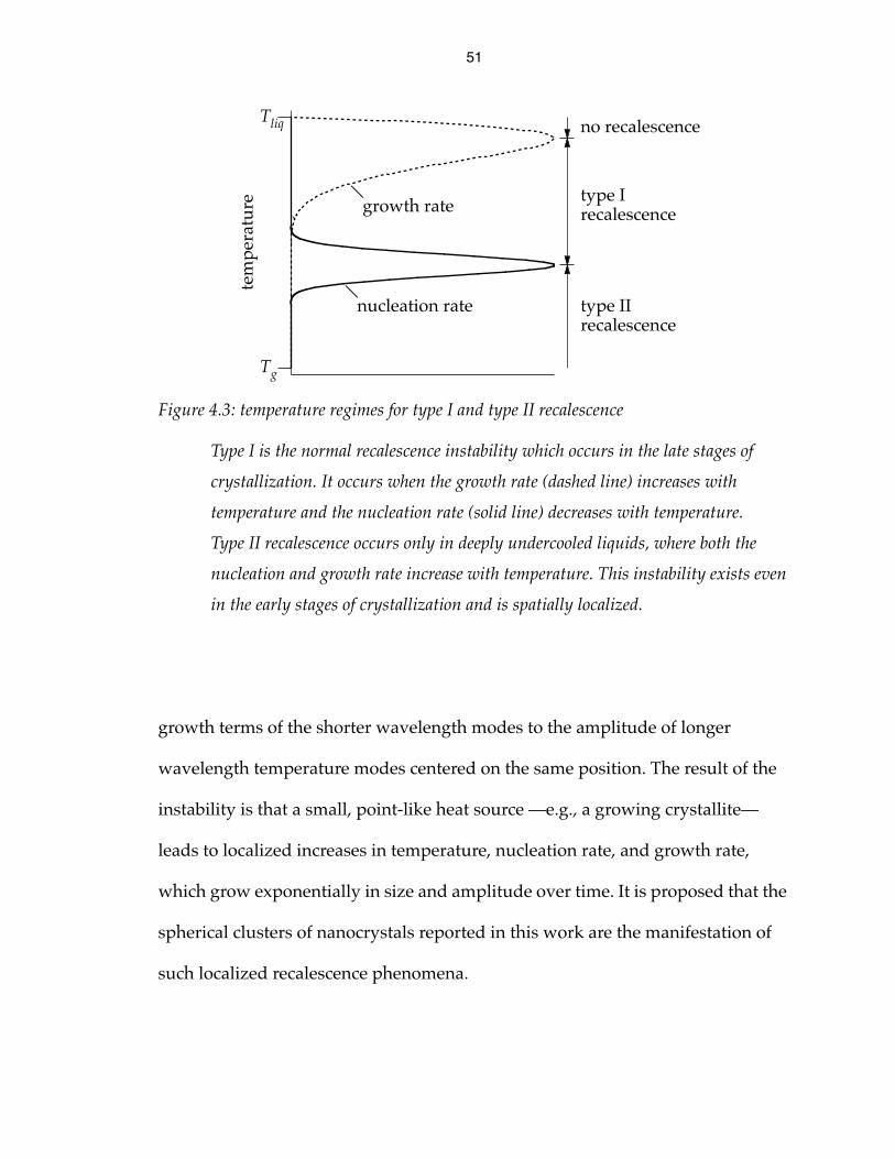
Figure 4.3: temperature regimes for type I and type II recalescence

Type I is the normal recalescence instability which occurs in the late stages of

crystallization. It occurs when the growth rate (dashed line) increases with

temperature and the nucleation rate (solid line) decreases with temperature.

Type II recalescence occurs only in deeply undercooled liquids, where both the

nucleation and growth rate increase with temperature. This instability exists even

in the early stages of crystallization and is spatially localized.

tem

pera

ture

Tliq

Tg

no recalescence

type Irecalescence

type IIrecalescence

nucleation rate

growth rate

52

The time required for the instability to manifest itself is the inverse of the positive

eigenvalue . Using classical nucleation theory for the homogeneous nucleation

rate (Eq. 4.5), with an interfacial tension of , the maximum temperature

derivative of the nucleation rate in Vit101 is . The heat

capacity, heat of crystallization and thermal diffusivity of Vit101 have been

measured as , and , respectively [36,37]. The

crystal growth rate can be estimated at from the typical size of the

nanocrystals in Fig. 3.8 (10 nm) and the time they had to grow (not more than 1 s).

With those values, the time constant for a feature size of 200 µm evaluates to

250 ms. Considering that the timescale for cooling the liquid to form a glass is on

the order of seconds in this alloy, this implies that the predicted recalescence

instability is significant in the crystallization kinetics of Vit101 during glass

formation.

Glass formation

In the process of glass formation, it is inevitable to pass through the deeply

undercooled liquid regime where the nucleation rate increases with temperature,

and encounter the type II recalescence instability. The effect of the recalescence is

to increase the size and number of crystals formed at a given external cooling rate,

increasing the critical cooling rate for glass formation. Furthermore, the localized

heat release from the few crystals which were nucleated and had the opportunity

to grow at high temperature —before the recalescence instability existed— causes

the recalescence to occur locally. At cooling rates above the critical cooling rate the

λ+

100mJ m2⁄

3 26×10 nuclei m3sK⁄

45J mol K⁄ 11.3kJ mol⁄ 5 6–×10 m2 s⁄

6 26–×10 m3 s⁄

53

recalescence is quenched by the surrounding liquid. As the cooling rate decreases,

the number and size of crystals nucleated at high temperature increases, and there

is more time for thermal conduction, so the localized recalescence events are more

closely spaced and grow to greater size, eventually overlapping. The overlap

reduces heat flow to the surrounding liquid, resulting in mutual enhancement of

the recalescence events. When the heat flow is insufficient to quench a

recalescence event, this recalescence event continues to grow, engulfing the

surrounding recalescence events, and ultimately leading to complete

crystallization.

In this proposed crystallization mechanism it is the interaction of the localized

recalescence events that triggers complete crystallization of the sample. Without

the interaction or the localized recalescence events, the transition from glass

formation to crystallization would be much more gradual, with a wide range of

cooling rates where partial crystallization is observed. The critical cooling rate for

glass formation would be lower, and not so well-defined. In isothermal

experiments too, recalescence causes the onset of crystallization to be sharper

than it would be without recalescence (type I recalescence can be compensated for

in a temperature-controlled experiment, but the localized type II recalescence can

not). In general, crystallization kinetics in this proposed crystallization

mechanism are characterized by an incubation time, where the amplitude and

size of the localized recalescence events are too small to be detected, followed by

rapid crystallization when the recalescence involves the entire sample.

54

5. Alloy Development

5.1. Requirements for glass formation

One of the reasons for studying the crystallization behavior of bulk glass forming

alloys is to use the knowledge so obtained in the search for new and improved

glass forming alloys. In this regard, the details of the crystallization kinetics are of

less interest than the composition dependence of the critical cooling rate. Based

on the discussion of crystal nucleation and growth kinetics in the previous

chapter, some general statements can be made about the requirements for a good

glass forming composition.

High reduced glass transition temperature

The reduced glass transition temperature plays a crucial role in

determining the glass forming ability of an alloy. To make a glass, the alloy must

be cooled from the thermodynamically stable liquid above the liquidus

temperature to below the glass transition temperature. The reduced glass

transition temperature not only gives the width of this temperature interval, it

also determines how close to the liquidus temperature the decreasing mobility in

the liquid starts to reduce the nucleation rate.

A high reduced glass transition temperature therefore leads to low nucleation

rates. If the reduced glass transition temperature is above 2/3, the rate of

Trg Tg Tliq⁄=

55

homogeneous nucleation is so low that it is negligible at laboratory time

scales [24].

Variations in the reduced glass transition temperature are largely due to the

variations in the liquidus temperature. The glass transition temperature scales

roughly with the binding energy of the alloy, and does not depend strongly on

composition [38]. The search for good glass forming alloys therefore starts with

low-lying liquidus surfaces, i.e., near deep eutectics.

Shift away from phases that nucleate easily

The eutectic indicates which liquid composition is most stable compared to the

competing crystalline phases under thermodynamic equilibrium conditions, i.e.,

at infinitely slow cooling rates. At finite cooling rates most liquids can be

undercooled significantly below their liquidus temperature before crystallization

sets in. The degree to which the liquid can be undercooled depends on the cooling

rate and the nucleation kinetics. At the critical cooling rate, the undercooling

diverges and the liquid can be undercooled to any temperature without

crystallizing.

If competing crystalline phases have different interfacial tensions with the liquid,

the degree to which they can be undercooled below their respective liquidus

temperatures will differ. Phases for which the interfacial tension with the liquid is

low can nucleate more easily, and will exhibit less undercooling, than those for

which the interfacial tension is higher [39].

56

The relevance of this effect for glass formation and its composition dependence is

illustrated in Fig. 5.1. As the cooling rate increases, the “non-equilibrium eutectic”

composition shifts away from the phases that exhibit less undercooling towards

those that can be undercooled more. The glass forming composition at the lowest

Figure 5.1: schematic non-equilibrium phase diagram of eutectic system

The liquidus curves in this phase diagram are shifted to lower temperatures to

account for the undercooling that occurs at finite cooling rates. Glass formation

occurs when the undercooling reaches the glass transition. The composition which

forms a glass at the lowest cooling rate is shifted, relative to the eutectic

composition, towards the phase with higher undercooling.

cooling rateglass formation

57

cooling rate where glass formation occurs, i.e., by definition the best glass forming

composition, is this “non-equilibrium eutectic” at that cooling rate.

The interfacial tension with the liquid is expected to be highest for simple crystal

structures, and lowest for topologically close-packed structures whose local

structure resembles that of the liquid [40].

Avoid heterogeneous nucleation

The resistance to crystallization of glass forming alloys depends at least partly on

the lack of homogeneous nucleation at high temperatures, where the crystal

growth rate is high. Heterogeneous nucleation sites increase the nucleation rate,

particularly at high temperatures, and are therefore deleterious to glass forming

ability. The effect of processing conditions —e.g., the use of a fluxing agent, choice

of atmosphere and crucible material, impurities in the alloying elements, and

general cleanliness of the apparatus— on glass forming ability of the alloy can be

explained by their effect on heterogeneous nucleation.

The use of a fluxing agent is of particular interest. For some bulk glass forming

alloys, notably those in the Pd-Ni-P family, the glass forming ability is greatly

improved by the use of a flux [41], boron oxide in the case of Pd-Ni-P. The effect of

the boron oxide flux in improving the glass forming ability of Pd-Ni-P is generally

attributed to the removal of heterogeneous nucleation sites from the melt and

their dissolution in the liquid boron oxide flux.

58

The role of oxygen impurities has also been studied. Deliberate contamination of

Zr52.5Ti5Cu17.9Ni14.6Al10 was found to cause crystallization at shorter times and

higher temperatures [42]. Throughout this work, particular care was taken to

keep the oxygen contamination level as low as possible.

Low mobility

To the extent that the glass transition temperature characterizes the mobility of

the liquid, the requirement of low mobility coincides with the requirement of a

high reduced glass transition. For some liquids, however, the mobility increase

above the glass transition is much more gradual than for others. According to

Angell [43], supercooled liquids can be classified as strong or fragile on the basis

of the temperature dependence, scaled to the glass transition temperature, of their

viscosity. In this context strong liquids, which have lower mobility, are expected

to be better glass formers.

Applying this principle to alloy development is impractical, because determining

the temperature dependence of the viscosity of an alloy requires extensive

characterization. It is far simpler to measure the glass forming ability directly.

Control phase separation

The effect of phase separation on glass forming ability is ambiguous. Phase

separation could in principle be beneficial for glass formation, by inhibiting

crystal growth and necessitating more nucleation; if crystals nucleated in one of

59

the decomposed phases do not grow into the other decomposed phase, separate

crystals need to be nucleated in each of the decomposed regions. Phase separation

may not affect glass forming ability at all, if the critical cooling rate is limited by a

process that occurs before phase separation occurs. But phase separation could

easily ruin the glass forming ability of an alloy: in all likelihood, at least one of the

two complementary composition shifts involved in phase separation is towards a

poorer glass forming composition.

Whether its effects are desired or undesired, if phase separation affects the glass

forming ability of an alloy, the composition dependence of the crystallization

behavior is complicated by the fact that the composition is no longer spatially

uniform and changes over time. Straightforward assumptions about the effects of

composition changes on crystallization behavior, e.g., that changing the

composition away from a crystalline phase disrupts the crystallization of that

phase, break down. So if phase separation plays a part in the crystallization

behavior of an alloy, it is important to recognize that fact to avoid drawing the

wrong conclusions.

5.2. Empirical optimization

The object of alloy development is to minimize some cost function defined on a

composition space. The cost function represents the trade-off between the various

properties that are desired or undesired for the alloy. In order for the optimization

to be mathematically meaningful the cost function must be scalar, so that an

60

ordering relation is defined. In the context of bulk metallic glasses, the cost

function to be optimized is the inverse of the glass forming ability.

Physical insight and theoretical predictions can be invaluable aids for this

optimization problem, by suggesting promising starting points and by

interpreting and extrapolating measured data. But at some point the properties

must be measured for a number of alloy compositions to verify or determine

experimentally which composition is most desirable. These measurements are

often time consuming and expensive, so it is worthwhile to choose an

optimization algorithm that keeps the number of measurements to a minimum.

Brute force

Conceptually, the optimal composition in an alloy system is determined by

measuring every possible composition and choosing the one that gave the best

result. In practice, only a finite number of measurements can be performed. Still, a

brute force approach, where a large number of samples spanning the entire

composition space is measured, is always an option. In fact, while other methods

may be more efficient at finding a local optimum, without a priori knowledge

about the function to be optimized a brute force search is the only method certain

to find a global optimum.

According to the Nyquist sampling theorem [44], the minimum feature size that is

certain to be detected is twice the spacing between the samples. The number of

samples required for a brute force search is therefore inversely proportional to the

61

Nth power of the minimum feature size, where N is the dimensionality of the

space to be searched. Since the dimensionality of the composition space for an

n-component system is , this number rapidly becomes prohibitively large* as

the number of components increases. The brute force approach is appropriate

only if the space to be searched is small, if the measurements are quick and cheap,

or if all other options have been exhausted. Alloy development with

multi-component alloys does not normally fall under any of these categories.

Steepest descent

Instead of attempting to measure the glass forming ability for every composition

in an alloy system to find the best glass former, more efficient strategies proceed

towards a local optimum by focusing on the directions in composition space in

which the glass forming ability improves most rapidly. These strategies require

some —ideally quantitative— information about the local composition

dependence of the glass forming ability. When such information is not available

directly from experiments and/or theory, the composition dependence can be

approximated by linearly extrapolating from measurements on a small number of

individual compositions, i.e., by determining the gradient.

* For example, there are more than 10000 compositions in a grid spaced at 5%

composition intervals for a 5-component system. For a grid spaced at 1% intervals the

number is approximately , and for a 5% grid in an 8-component system it is

. In general, in an n-component system there are compositions spaced

at intervals of on a grid with the symmetry of the composition space.

n 1–

18

×10

36

×10 p k+k

------------k 1=

n 1–∏

1p---

62

The benefit that can be gained by using a steepest descent strategy for optimizing

composition depends on the accuracy with which the composition dependence

can be extrapolated, and on the complexity of the “glass forming ability

landscape.” The difference in glass forming ability between the compositions

used for the extrapolation must be larger than the uncertainty on the

measurement, otherwise the resulting gradient is meaningless. This requirement

imposes a lower bound on the composition difference between the alloys used for

the extrapolation. On the other hand, the complexity of the landscape imposes an

upper bound on the distance over which the gradient is accurate. A steepest

descent strategy is most effective in simple landscapes, where little information is

needed to specify the composition dependence of the glass forming ability.

Based on the correlation between glass forming ability and the reduced glass

transition temperature, whose composition dependence follows that of the

liquidus temperature, it is not unreasonable to expect the glass forming ability

landscape to be rather similar to the liquidus surface in a eutectic phase diagram,

illustrated in Fig. 5.2. In this analogy, the glass forming ability is limited by the

primary crystallizing phase, and improves monotonically as the composition is

shifted away from the composition of this crystalline phase until a different phase

becomes the primary crystallizing phase. The landscape is then a smoothly

varying surface, except where the surfaces for different primary crystallizing

phases intersect, there the slope is discontinuous. A steepest descent strategy

should work relatively well in such a landscape.

63

Discussion

The results from Fig. 3.4 on page 27, however, are inconsistent with such a simple

glass forming ability landscape. The critical casting thickness of Vit101 displays a

local minimum in the middle of a good glass forming region, where a local

Figure 5.2: schematic illustration of ternary eutectic phase diagram

The liquidus projection is shown in the base plane.

64

maximum is expected. No explanation for this surprising result has been

established yet. One possibility is that where there is a transition from one

primary crystallizing phase to another, the crystallization of one phase is

accelerated by the crystallization of the other phase. In the discussion leading up

to “Spatially localized nucleation” on page 47, such feedback effects were put

forward to explain the microstructure described in chapter 3. It is possible that the

feedback effect results not purely from temperature dependence but also involves

composition dependence and partitioning.

Whatever the cause of the unexpected result in Fig. 3.4, it clearly indicates that the

glass forming ability landscape in the region of interest is complex, and contains

features which were overlooked in the work of Lin [45], where compositions were

spaced 2 to 5% apart. Figure 3.4 shows that the glass forming ability can change

significantly with composition changes as small as 1%. The complexity of the

landscape disrupts the steepest descent optimization strategy, while the small

feature size drastically increases the number of samples required for a

comprehensive brute force search. As yet, our understanding of the crystallization

process —and knowledge of the thermodynamic properties— in these

multicomponent bulk glass forming alloys is insufficient to predict the

crystallization behavior at the level of detail required to move alloy development

past empirical optimization.

65

6. Annealing

The stability against crystallization at temperatures slightly above the glass

transition enables bulk metallic glasses to be processed more like plastics than like

metals, for example by extrusion of amorphous powders [46]. Any discussion of

crystallization behavior of metallic glasses is therefore incomplete if it does not

address crystallization upon heating of amorphous samples.

6.1. Experimental results

Small angle X-ray scattering (SAXS)

The crystallization behavior of Vit101 samples during annealing was observed in

situ by small angle X-ray scattering. The evolution of the radial average of the

scattering intensity with time is shown in Fig. 6.1 and Fig. 6.2, for two different

temperatures. The Q value on the horizontal axis in these plots is the modulus of

the scattering vector. The as-prepared samples exhibit only surface scattering,

which drops off rapidly at increasing Q and is insignificant for Q values greater

than 0.05 Å. During annealing, the scattered intensity increases over time and an

interference maximum develops at Q=0.073 Å-1 for the sample annealed at 665 K

and at Q=0.036 Å-1 for the sample annealed at 769 K. In the sample annealed at

the higher temperature, the signal changes shape as well, with a shoulder

developing around Q=0.07 Å-1.

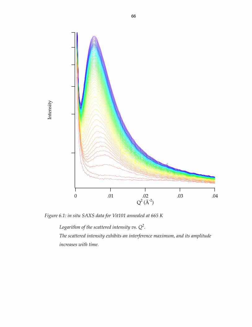
66

Figure 6.1: in situ SAXS data for Vit101 annealed at 665 K

Logarithm of the scattered intensity vs. Q2.

The scattered intensity exhibits an interference maximum, and its amplitude

increases with time.

Inte

nsit

y

.04.03.02.010Q2 (Å-2)

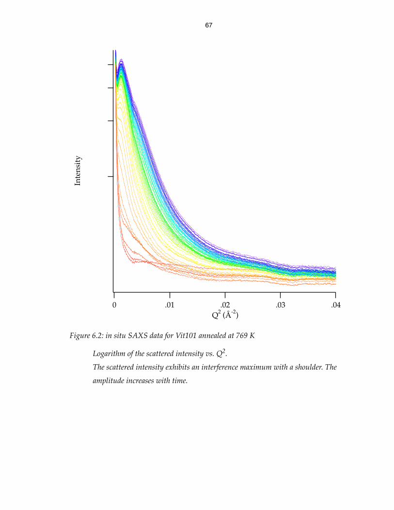
67

Figure 6.2: in situ SAXS data for Vit101 annealed at 769 K

Logarithm of the scattered intensity vs. Q2.

The scattered intensity exhibits an interference maximum with a shoulder. The

amplitude increases with time.

Inte

nsit

y

.04.03.02.010Q2 (Å-2)

68

Differential scanning calorimetry (DSC)

Vit101 samples that were annealed at temperatures similar to those in the small

angle X-ray scattering experiments were subsequently studied by DSC [47].

Figure 6.3 shows DSC traces of an as-prepared sample and several annealed

samples. There are three distinct exothermic events in the DSC trace of the

as-prepared sample. In the annealed samples one or more of the peaks have

become smaller or disappeared entirely, indicating that the crystallization events

corresponding to those peaks have already occurred during the annealing.

6.2. Discussion

Small angle scattering yields information about the size and spacing of the

scattering structures. According to the Guinier approximation for small angle

scattering from a particle, the slope in a plot of the logarithm of the scattered

intensity vs. Q squared is proportional to the size of the particle. A correlated

arrangement of scattering particles will result in an interference maximum in the

scattered intensity. The inverse of the Q value where this maximum occurs is a

typical spacing of the particles.

The SAXS data was analyzed using the following ad hoc expression for the radial

average scattered intensity as a function of Q:

, (6.1)C1 C2QnC3

1µ2 Q2–

σ------------------

exp+

-------------------------------------------Rg

2Q2

3-------------–

exp+ +

69

where the parameters , and their evolution with annealing

time, were obtained from non-linear least squares regressions. The first term

accounts for a constant shift in the baseline, the second term accounts for surface

scattering (ideally with an exponent of -2), and the third term embodies the

Guinier approximation for scattering from the crystals, multiplied by an envelope

function to account for interference. are the intensities for the three

Figure 6.3: DSC traces of annealed Vit101 samples

The direction for exothermic events is down. Traces are offset by multiples of 1 W/g

to separate them from eachother.

650 700 750 800 850

-5

-4

-3

-2

-1

0

1

691 K, 16 h

669 K, 16 h

723 K, 15 h

as-prepared

748 K, 3.5 h

701 K, 24 h

heat

flo

w (

W/g

)

temperature (K)

C1 C2 n C3 Rg µ σ, , , , , ,

C1 C2 C3, ,

70

terms, n is the adjustable exponent in the surface scattering term, µ is

(approximately) the position of the interference maximum, σ is a shape factor for

the envelope function , and is the Guinier radius of

gyration.

The evolution of the radius of gyration thus obtained for samples annealed at

different temperatures is plotted in Fig. 6.4. It increases initially, but surprisingly

decreases again in the later stages. At higher annealing temperatures this decrease

is more pronounced and occurs after shorter annealing times. It was noted that in

Fig. 6.2 a shoulder develops precisely where the slope should be measured to

evaluate the Guinier radius. It is concluded that the decrease in is related to

the development of this shoulder rather than a decrease in the size of the crystals

that grew earlier.

When the temperatures of the SAXS experiments are compared with the DSC

trace of the as-prepared sample, the interpretation of the shoulder in the SAXS

data and of the decrease in becomes clear. The first exothermic event in the

DSC trace would have occurred in each of the SAXS experiments. In the SAXS

experiments at 754 K and at 769 K, the second exothermic event in the DSC trace

would have passed as well. The DSC trace for the sample annealed at 669 K

reveals that even at this lower temperature the second event would probably have

begun on the time scale of the SAXS experiments.

Thus, during each of the SAXS experiments two separate crystallization processes

contributed to the evolution of the scattered intensity. The superposition of these

1µ2 Q2–

σ------------------

exp+

1–Rg

Rg

Rg

Rg

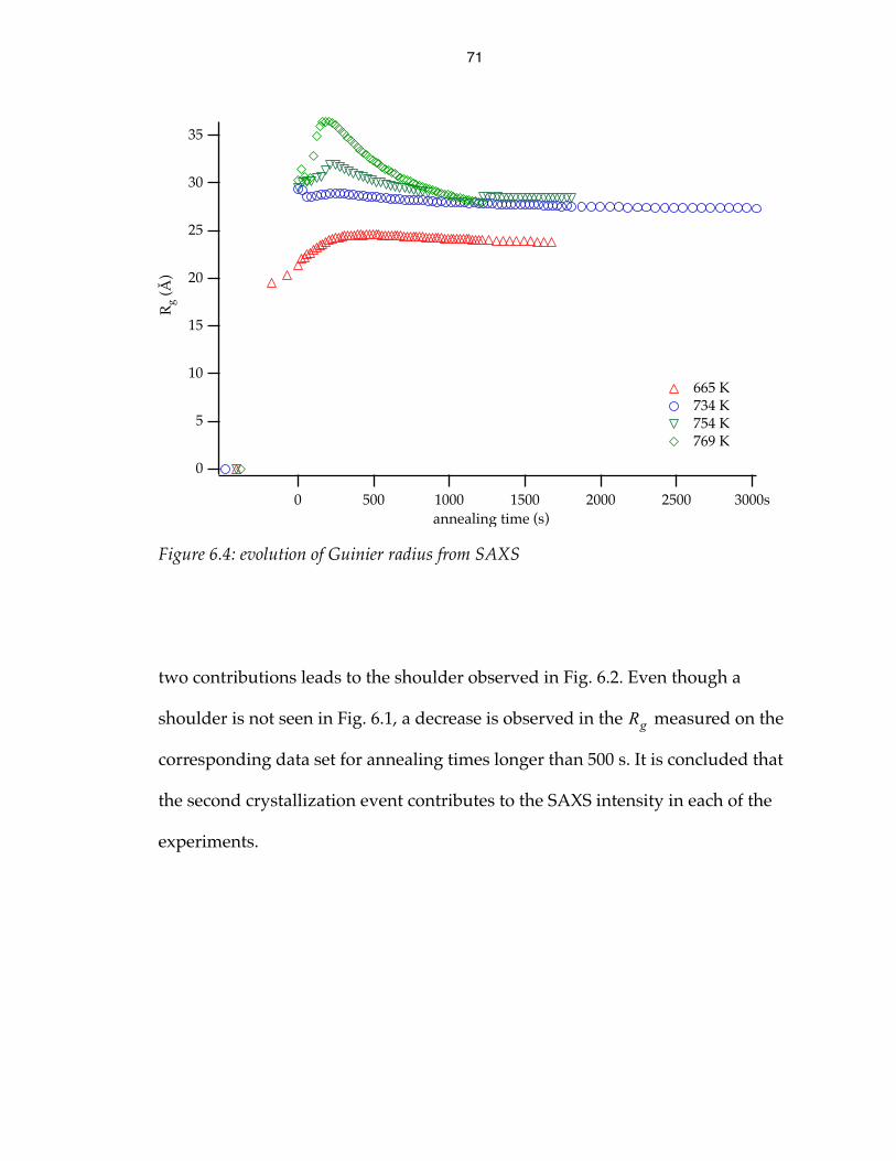
71

two contributions leads to the shoulder observed in Fig. 6.2. Even though a

shoulder is not seen in Fig. 6.1, a decrease is observed in the measured on the

corresponding data set for annealing times longer than 500 s. It is concluded that

the second crystallization event contributes to the SAXS intensity in each of the

experiments.

Figure 6.4: evolution of Guinier radius from SAXS

35

30

25

20

15

10

5

0

Rg

(Å)

3000s25002000150010005000annealing time (s)

665 K 734 K 754 K 769 K

Rg

72

7. Summary

The solidification microstructure in wedge-shaped castings was investigated, for

a series of alloys with compositions systematically varied around

Cu47Ni8Ti34Zr11. Near the critical thickness for glass formation, a spatially

inhomogeneous dispersion of nanocrystals was observed, where spherical

regions contain a much higher density of nanocrystals than the surrounding

material. This microstructure is inconsistent with the prevalent theories for

crystallization in metallic glasses, which predict a spatially uniform distribution

of crystals.

The spatial localization of the nucleation density was attributed to a recalescence

instability. When the heat of crystallization was included in the Fourier heat flow

equation, coupling the crystal nucleation and growth rates to the heat flow

problem, stable solutions were found only under certain conditions. In deeply

undercooled liquids, where the nucleation rate increases with temperature, these

conditions are never met, and recalescence can occur locally, triggered by a small

fluctuation in the early stages of the crystallization process. It was argued that

because the localized recalescence events and their interaction accelerate

crystallization, they are important in determining the glass forming ability as well

as the microstructure of these alloys.

The composition dependence of the critical thickness for glass formation,

determined from the observed microstructures, and in situ small angle scattering

73

results acted as a reminder that crystallization in glass forming alloys is a complex

process involving several competing crystalline phases.

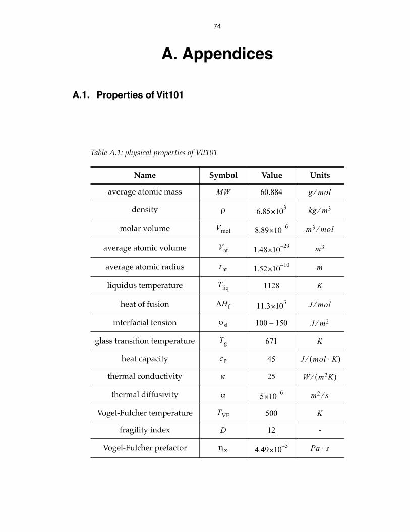
74

A. Appendices

A.1. Properties of Vit101

Table A.1: physical properties of Vit101

Name Symbol Value Units

average atomic mass

density

molar volume

average atomic volume

average atomic radius

liquidus temperature

heat of fusion

interfacial tension

glass transition temperature

heat capacity

thermal conductivity

thermal diffusivity

Vogel-Fulcher temperature

fragility index -

Vogel-Fulcher prefactor

MW 60.884 g mol⁄

ρ 6.85 3×10 kg m3⁄

Vmol 8.89 6–×10 m3 mol⁄

Vat 1.48 29–×10 m3

rat 1.52 10–×10 m

Tliq 1128 K

∆Hf 11.3 3×10 J mol⁄

σsl 100 150– J m2⁄

Tg 671 K

cP 45 J mol K⋅( )⁄

κ 25 W m2K( )⁄

α 5 6–×10 m2 s⁄

TVF 500 K

D 12

η∞ 4.49 5–×10 Pa s⋅

75

A.2. Solutions to the Fourier heat flow equation

Application of spectral theory

The Laplacian appearing in the Fourier heat flow equation (Eq. 2.1) is a linear

operator on the Hilbert space of all functions which satisfy the boundary

conditions. The Laplacian therefore has a spectral representation [48], which can

be used to solve the Fourier heat flow equation. With rectangular boundary

conditions, the spectral representation of the Laplacian is the familiar Fourier

transform*. The spectral representation of the Laplacian transforms the heat flow

equation, a partial differential equation in , into an infinite set of first-order

ordinary differential equations in the spectral coefficients :

(A.1)

where is the improper eigenvalue of the Laplacian corresponding to the

improper eigenfunction , i.e., . The solution to the Fourier

heat flow equation projected on these eigenfunctions is:

(A.2)

The solutions of Eq. A.1 for the coefficients are exponentials decaying with a

time constant :

(A.3)

* Spectral theory provides the generalization of the Fourier transform method for solving

the heat flow equation with boundary conditions other than rectangular or infinite.

T x t,( )

θk t( )

t∂

∂θk αk2θk t( )–=

k2–

Tk x( ) Tk x( )∇2 k2– Tk x( )=

T x t,( ) θk t( )Tk x( )k∑=

θk t( )

τ 1 αk2( )⁄=

θk t( ) θk 0( )e αk2t–=

76

Thus, a general solution to the Fourier heat flow equation is given by

(A.4)

where the boundary conditions are represented by the form of the eigenfunctions

and the initial conditions determine the initial values of the spectral

coefficients.

E.g., in one dimension, spectral representation is a Fourier series:

with (A.5)

and the solution to the heat flow equation can be written as

. (A.6)

Unfortunately, Fourier expansions do not converge very well near discontinuities,

a fact which limits the usefulness of this expression in describing the early stages

of heat flow. In the late stages, the short wavelength terms have all decayed away,

and the fundamental harmonic dominates, decaying with a time constant

.

Heat flow in a flat plate

For a plate of constant thickness where the width and height are much greater

than the thickness, cooled from the surface, the temperature profile is to a good

T x t,( ) θk 0( )e αk2t– Tk x( )k∑=

Tk x( ) θk 0( )

T x t,( ) θk t( ) kx( )sink∑= θk t( )

12L------ T x t,( ) kx( )sin xd

0

L

∫=

T x t,( )1

2L------ e αk2t– T x( )

t 0=kx( )sin xd

0

L

∫

kx( )sink∑=

τ L2 π2α( )⁄=

77

approximation one-dimensional. The initial condition is and the

boundary conditions are . Eq. A.6 then results in

. (A.7)

Fig. A.1 shows the evolution over time of this temperature profile with typical

values for the physical parameters.

Heat flow at a semi-infinite wall

In the early stages of any heat flow problem where the initial temperature is

uniform, the temperature remains uniform except near the surface. If the surface

is planar or if its radius of curvature is sufficiently large, the heat flow near the

surface can be treated as a limit of the previous case where . The

summation in Eq. A.7 is then replaced by an integral:

, (A.8)

which in this case can be solved analytically:

, (A.9)

resulting in the final answer:

. (A.10)

This temperature profile, with the same parameters as in Fig. A.1, is displayed in

Fig. A.2.

T x( )t 0=

T∞=

T t( )x 0=

T t( )x L=

T0= =

T x t,( ) T0 T∞ T0–( )1

kL------e αk2t– kx( )sin

k 2n 1+( )πL

------------------------=

∑+=

L ∞→

T x t,( ) T0 T∞ T0–( )1k---e αk2t– kx( )sin kd

0

∞

∫+=

1k---e αk2t– kx( )sin kd

0

∞

∫ e αk2t– kx( )sin kd0

∞

∫

xd∫ ex2

4αt---------–

xd∫ erf x

4αt-------------( )= = =

T x t,( ) T0 T∞ T0–( )erf x

4αt-------------( )+=

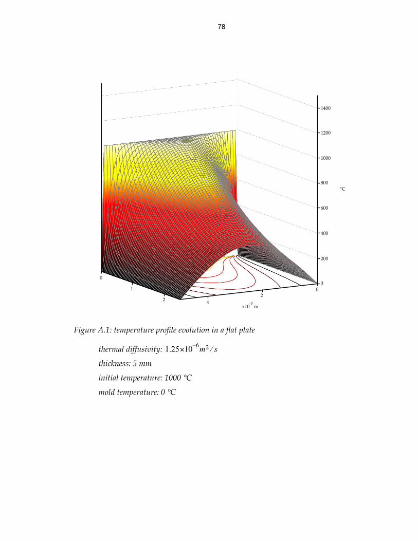
78

Figure A.1: temperature profile evolution in a flat plate

thermal diffusivity:

thickness: 5 mm

initial temperature: 1000 °C

mold temperature: 0 °C

0

1

2

02

4

0

200

400

600

800

1000

1200

1400

°C

x10-3

m

1.25 6–×10 m2 s⁄

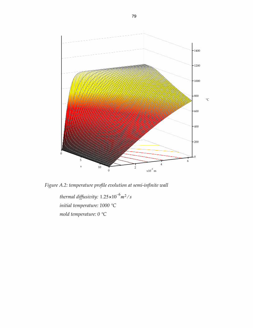
79

Figure A.2: temperature profile evolution at semi-infinite wall

thermal diffusivity:

initial temperature: 1000 °C

mold temperature: 0 °C

0

5

100

24

60

200

400

600

800

1000

1200

1400

°C

x10-3

m

s

1.25 6–×10 m2 s⁄

80

A.3. Geometry of composition spaces

The composition of an n-component alloy is completely specified by the amounts

of each of the n components present in the alloy. However, the total amount of the

alloy does not influence the composition, so there are compositional degrees

of freedom. Mathematically this is expressed as a normalization: the

n-dimensional vector space of the amount of each of the components is projected

onto the dimensional surface where the norm is equal to 1.

The choice of the normalization function is somewhat arbitrary. It corresponds to

the choice of units for the amounts of the different components, although in

principle other normalization functions (without physical meaning) could also be

considered. A different norm function will define a projection onto a different

composition space. For example, compositions are commonly expressed as either

mole fractions or mass fractions, and some stretching is necessary to convert a

graphical representation of one to the other. In this case, both normalization

functions are linear, so the transformation from one to the other is linear in the

original n-dimensional space. As a result, a straight line remains a straight line in

the dimensional space, even though angles and relative distances change.

This is not true if —in the chosen units, volume for example— the total amount is

not conserved on mixing, which corresponds to a non-linear normalization

function.

The constraint that the amounts of each of the components must be positive

translates into a set of n symmetric linear bounds on the dimensional

n 1–

n 1–

n 1–

n 1–

81

composition space. The physically meaningful compositions are therefore

constrained to the dimensional generalization of a tetrahedron. As shown in

Fig. A.3, the physically meaningful compositions are therefore constrained to the

linear interval [0,1] for a 2-component system, to an equilateral triangle for a

3-component system, to a regular tetrahedron for a 4-component system, etc…

The full dimensionality of the composition space of a system with 4 or more

components is hard to visualize in 2 dimensions. Such composition spaces are

usually represented by a projection onto a pseudo-ternary diagram, either by

ignoring some of the components or grouping several together at one of the

vertices of the triangle.

The highly symmetrical nature of composition spaces (and the difficulty of

visualizing the full dimensionality of the composition space of a system with

more than 4 components) illustrate that although the composition space has only

degrees of freedom, it is often more convenient to think of it as the

projection of an n-dimensional space.

n 1–

n 1–

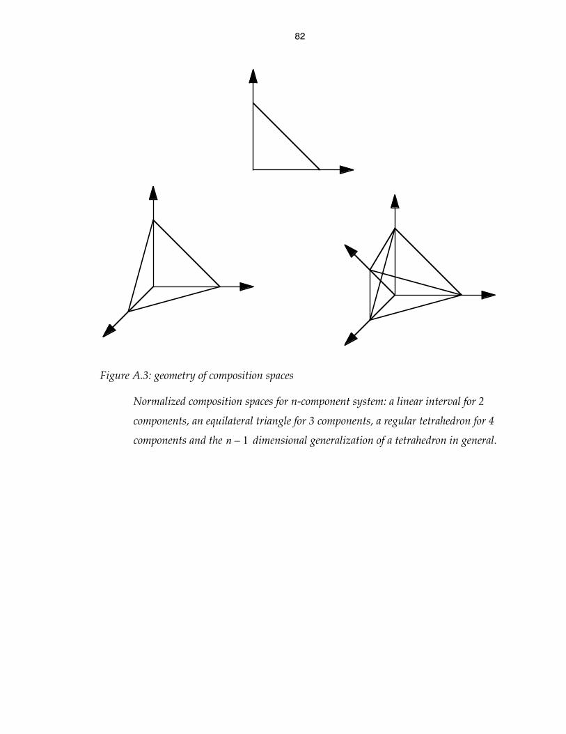
82

Figure A.3: geometry of composition spaces

Normalized composition spaces for n-component system: a linear interval for 2

components, an equilateral triangle for 3 components, a regular tetrahedron for 4

components and the dimensional generalization of a tetrahedron in general.n 1–

83

References

1. C. A. Angell, Science 267, 1924 (1995).

2. Binary Alloy Phase Diagrams; Eds. T. B. Massalski, H. Okamoto, P. R.

Subramanian, L. Kacprzak (William W. Scott, Jr., ASM International, 1990).

3. Yunus A Çengel, Heat Transfer: A Practical Approach (McGraw-Hill, 1998).

4. F. Press and R. Siever, Understanding Earth (Freeman, 1997), p. 78.

5. R. Cotterill, The Cambridge Guide to the Material World (Cambridge University

Press, 1985), Chap. 11.

6. H.-G. Elias, An Introduction to Plastics (VCH, 1993), Chap. 4.

7. W. Klement, R. Willens, and P. Duwez, Nature 187, 869 (1960).

8. H. L. Luo and P. Duwez, Appl. Phys. Lett. 2, 21 (1963).

9. P. Duwez, R. Willens, and R. C. Crewdson, J. Appl. Phys. 36, 2267 (1965).

10. P. Duwez and S. C. H. Lin, J. Appl. Phys. 38, 4096 (1967).

11. N. DeCristofaro, MRS Bulletin 23, 50 (1998).

12. A. Inoue, T. Zhang, and T. Masumoto, Mater. Trans. JIM 31, 425 (1990).

13. T. Zhang, A. Inoue, and T. Masumoto, Mater. Trans. JIM 32, 1005 (1991).

14. A. Peker and W. L. Johnson, Appl. Phys. Lett. 63, 2342 (1993).

15. A. Inoue, N. Nishiyama, and H. Kimura, Mater. Trans. JIM 38, 179 (1997).

16. C. C. Hays, J. Schroers, U. Geyer, S. Bossuyt, N. Stein, and W. L. Johnson,

Materials Science Forum 343-3, 103 (2000).

17. X. H. Lin and W. L. Johnson, J. Appl. Phys. 78, 6514 (1995).

18. J. T. Armstrong, Microbeam Analysis 4, 177 (1995).

19. J. Schroers, unpublished research.

84

20. C. C. Hays, unpublished research.

21. B. E. Warren, X-ray Diffraction (Addison-Wesley, 1969; Dover, 1990), Chap. 10.

22. B. E. Warren, X-ray Diffraction (Addison-Wesley, 1969; Dover, 1990), Chap. 13.

23. D. Turnbull and M. H. Cohen, J. Chem. Phys. 29, 1049 (1958).

24. D. Turnbull, Contemp. Phys. 10, 473 (1969).

25. J. W. Christian, The Theory of Transformations in Metals and Alloys (Pergamon),

Chap. 10.

26. K. F. Kelton, Solid State Phys. 45, 75 (1991).

27. A. Masuhr, Ph. D. Thesis, California Institute of Technology, 1999.

28. D. A. Porter and K. E. Easterling, Phase Transformations in Metals and Alloys

(Chapman & Hall, 1992), Chap. 4.

29. Y. J. Kim, R. Busch, W. L. Johnson, A. J. Rulison, and W. K. Rhim, Appl. Phys.

Lett. 68, 1057 (1996).

30. D. R. Askeland, The Science and Engineering of Materials (Chapman & Hall,

1990).

31. J. C. Foley, D. R. Allen, and J. H. Perepezko, Scr. Mater. 35, 655 (1996).

32. R. Busch, S. Schneider, A. Peker, and W. L. Johnson, Appl. Phys. Lett. 67, 1544

(1995).

33. S. Schneider, P. Thiyagarajan, and W. L. Johnson, Appl. Phys. Lett. 68, 493

(1996).

34. J. F. Löffler and W. L. Johnson, Appl. Phys. Lett. 76, 3394 (2000).

35. K. F. Kelton, Philos. Mag. Lett. 77, 337 (1998).

36. S. C. Glade, R. Busch, D. S. Lee, W. L. Johnson, R. K. Wunderlich, and H. J.

Fecht, J. Appl. Phys. 87, 7242 (2000).

85

37. R. K. Wunderlich, D. S. Lee, W. L. Johnson, and H. J. Fecht, Phys. Rev. B 55, 26

(1997).

38. H. A. Davies, Phys. Chem. Glasses 17, 159 (1976).

39. F. Spaepen and D. Turnbull, Rapidly Quenched Met. 2, 205 (1976).

40. D. Holland-Moritz, J. Schroers, D. M. Herlach, B. Grushko, and K. Urban, Acta

Mater. 46, 1601 (1998).

41. H. W. Kui, A. L. Greer, and D. Turnbull, Appl. Phys. Lett. 45, 615 (1984).

42. X. H. Lin, W. L. Johnson, and W. K. Rhim, Mater. Trans. JIM 38, 473 (1997).

43. C. Angell, J. Phys. Chem. 100, 13211 (1996).

44. R. B. Ash, Information Theory (Wiley, 1965; Dover, 1999), Chap. 8.

45. X. H. Lin, Ph. D. Thesis, California Institute of Technology, 1996.

46. J. C. Foley, D. J. Sordelet, and T. A. Lograsso, in Mat. Res. Soc. Proc. 554, 199

(Materials Research Society, 1999), Eds. W. L. Johnson, A. Inoue and C. T. Liu;

D. J. Sordelet, private communication.

47. S. C. Glade, J. F. Löffler, S. Bossuyt, W. L. Johnson, and M. K. Miller, to be

published in J. Appl. Phys.

48. B. Friedman, Principles and Techniques of Applied Mathematics (Wiley, 1956;

Dover, 1990).