Microstructural modeling of cross-linked fiber network ... · Microstructural modeling of...

Microstructural modeling of cross-linked fiber network embedded in continuous matrix

by

Lijuan Zhang

A Thesis Submitted to the Graduate

Faculty of Rensselaer Polytechnic Institute

in Partial Fulfillment of the

Requirements for the degree of

DOCTOR OF PHILOSOPHY

Major Subject: MECHANICAL ENGINEERING

Approved by the Examining Committee:

_________________________________________ Mark S. Shephard, Thesis Adviser

_________________________________________ Catalin R. Picu, Thesis Adviser

_________________________________________ Antoinette M. Maniatty, Member

_________________________________________ David T. Corr, Member

_________________________________________ Victor H. Barocas, Member

Rensselaer Polytechnic Institute Troy, New York

December 2013

ii

© Copyright 2013

by

Lijuan Zhang

All Rights Reserved

iii

CONTENTS

LIST OF TABLES ............................................................................................................ vi LIST OF FIGURES ......................................................................................................... vii ACKNOWLEDGMENT ................................................................................................... x ABSTRACT ..................................................................................................................... xi 1. Background in soft tissue modeling and thesis organization ....................................... 1

1.1 Background and motivation ............................................................................... 1

1.2 Mechanical behaviors of soft connective tissues: structure – function relationship ......................................................................................................... 2

1.3 Computational model developments .................................................................. 4

1.4 Organization of dissertation ............................................................................... 8

2. Non-manifold geometry modeling and mesh generation .......................................... 10

2.1 Introduction and overview of the coupled model ............................................ 10

2.2 Voronoi fiber network generation .................................................................... 12

2.3 Non-manifold geometric modeling using Parasolid ........................................ 15

2.3.1 Introduction to non-manifold and manifold models ............................ 15

2.3.2 General description of construction of the non-manifold geometric model .................................................................................................... 16

2.3.3 Constructing the non-manifold model of fiber and matrix .................. 19

2.4 Multi-dimensional mesh generation ................................................................. 25

3. Finite element analysis of the coupled fiber-matrix model ....................................... 29

3.1 Material model representing embedded fiber and matrix ................................ 29

3.2 Nonlinear finite element formulation of the coupled fiber-matrix model ........ 30

3.2.1 Newton-Raphson iterative approach .................................................... 31

iv

3.2.2 Nonlinear finite element equations ...................................................... 32

3.2.3 Strain-displacement relationship for three dimensional matrix elements .............................................................................................................. 36

3.2.4 Nonlinear finite element formulation for one dimensional truss element

.............................................................................................................. 38

3.3 Matrix and vector assembling of coupled linear tetrahedron and truss ........... 41 4. Mechanical behaviors of the RVE composite ........................................................... 44

4.1 Problem definition ............................................................................................ 44

4.1.1 Boundary conditions ............................................................................ 44

4.1.2 Nomenclature ....................................................................................... 45

4.1.3 Material constitutive models ................................................................ 46

4.2 Overall RVE constitutive response .................................................................. 49

4.2.1 Overall RVE constitutive response with nonlinear materials .............. 49

4.2.2 Comparison between the coupled model and parallel model............... 53

4.2.3 RVE constitutive response with linear material models ...................... 58

4.2.4 Discussion ............................................................................................ 60

4.3 Effect of fiber network on matrix – the case of linear material models ........... 61

4.3.1 Inhomogeneous stress distribution in the matrix ................................. 61

4.3.2 Probability distribution function of matrix element stresses................ 63

4.3.3 Locations of stress concentration in the matrix material ..................... 65

4.4 Effect of matrix material on the fiber network – the case of linear material models .............................................................................................................. 67

4.5 Effective elastic modulus and Poisson ratio of the composite ......................... 70

4.6 Conclusion ....................................................................................................... 75

5. Volume averaging-based multiscale model ............................................................... 77

v

5.1 Introduction ...................................................................................................... 77

5.2 Scale linking between macroscopic and microscopic scales ........................... 78

5.2.1 Downscaling – RVE boundary deformation ........................................ 78

5.2.2 Scaling .................................................................................................. 79

5.2.3 Upscaling ............................................................................................. 80

5.3 Governing equations ........................................................................................ 80

5.4 Relating the microscopic scale to the macroscopic scale................................. 82

5.5 Example ........................................................................................................... 83

5.6 Conclusion ....................................................................................................... 86

6. Conclusion and future work ....................................................................................... 87

6.1 Conclusion ....................................................................................................... 87

6.2 Future work ...................................................................................................... 89 7. Reference ................................................................................................................... 91 Appendix A ...................................................................................................................... 97

vi

LIST OF TABLES

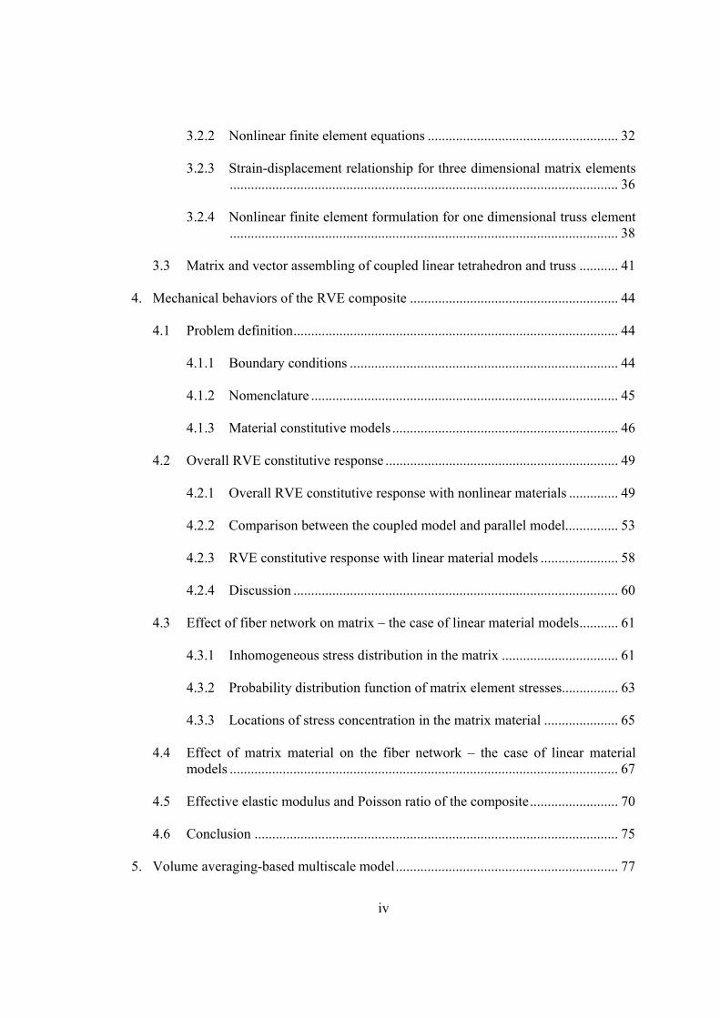
Table 1.1: Mechanical properties and associated biochemical data of some representative organs mainly consisting of soft connective tissues. ......................................................... 2 Table 2.1: Body ~ Region adjacent relationships. ........................................................... 22 Table 2.2: Region ~ Shell adjacent relationships. ........................................................... 23 Table 2.3: Shell ~ Face adjacent relationships. ............................................................... 23 Table 2.4: Shell ~ (Wire) Edge adjacent relationships. ................................................... 23 Table 2.5: Face ~ Loop adjacent relationships. ............................................................... 23 Table 2.6: Loop ~ Edge adjacent relationships................................................................ 24 Table 2.7: Loop ~ Vertex adjacent relationships. ............................................................ 24 Table 2.8: Edge ~ Vertex adjacent relationships. ............................................................ 25 Table 3.1: Numbering of degree of freedoms .................................................................. 42 Table 4.1: Nomenclature. ................................................................................................ 46 Table 4.2: Initial properties of anisotropic Voronoi networks used with nonlinear material models. ............................................................................................................... 47 Table 4.3: Initial properties of isotropic Voronoi networks used with linear material models. ............................................................................................................................. 48

vii

LIST OF FIGURES

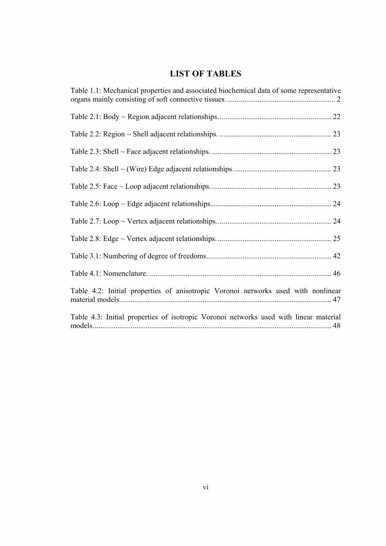
Figure 1.1: Scanning electron images of collagen fiber network at (a) 10,000X and (b) 50,000X magnification. ..................................................................................................... 3 Figure 1.2: Schematic diagram of a typical (tensile) stress-strain curve for skin showing the associated collagen fiber morphology. ........................................................................ 4 Figure 2.1: Schematic representation of the network: The red dots represent the points where the network intersects the model boundaries. ....................................................... 11 Figure 2.2: Work-flow demonstrating construction protocol for the coupled model. ..... 12 Figure 2.3: Procedure of Voronoi network generation. ................................................... 13 Figure 2.4: (a) Cellular body: Interior face shared by two regions – each side of the face is used by the associated region; (b) Multi-dimensional body: Three-dimensional region with embedded one-dimensional wire edges. .................................................................. 16 Figure 2.5: (a) Loops of a solid cube (only shows loops of three faces); (b) Vertex and wire loops. ........................................................................................................................ 18 Figure 2.6: Three fibers within matrix – blue lines and blue dots represent embedded fibers and fiber crosslinks (only one inner crosslink, the other three are boundary crosslinks); black lines and black dots represent cube edges and cube vertices. ............ 19 Figure 2.7: Faces of the studied case with red arrows representing face normal. ........... 20 Figure 2.8: Loops of the studies case: L1 through L6 are six loops bounding cube faces; L7, L8 and L9 are vertex loops. ....................................................................................... 21 Figure 2.9: Edges of the studied case: E1 through E12 are cube edges; E13, E14 and E15 are wire edges associated with embedded fibers. ............................................................ 21 Figure 2.10: Vertices of the studied case: V1 through V8 are cube vertices; V9, V10, V11 and V12 are vertices associated with fiber crosslinks in which V10 is an embedded vertex. .............................................................................................................................. 22 Figure 2.11: Illustration of the conforming multi-dimensional mesh and the mesh classification to the geometric model. ............................................................................. 26 Figure 2.12: Schematic showing the interior of the multi-dimensional mesh showing fibers (black lines) and meshed matrix (yellow elements with blue borders). ................ 26 Figure 2.13: 2D and 3D view of uniform multi-dimensional mesh (red dots represent fiber boundary crosslinks). .............................................................................................. 27

viii

Figure 2.14: 2D and 3D view of graded multi-dimensional mesh (red dots represent fiber boundary crosslinks. ........................................................................................................ 28 Figure 3.1: Illustration of a linear truss element. ............................................................. 39 Figure 3.2: A representative example of the coupled tetrahedron and truss members. ... 41 Figure 4.1: Symmetric boundary condition applied in in the uniaxial tensile test. ......... 44 Figure 4.2: (a) Averaged fiber stress, (b) averaged matrix stress, (c) averagedtotalstress, and (d) apparent RVE Poisson’s ratio vs. engineering strain ɛ for the coupled fiber-matrix model at varying values of Gm. ............................................................................ 52 Figure 4.3: Magnitude of stress contributions are different functions of whether simulation results are evaluated at constant total strain or constant total stress; (a) while matrix stress values increase in both cases, (b) fiber stresses show opposite trends for the two cases, where decreasing values for the constant-stress case demonstrates stress-shielding (by the matrix) at high shear modulus. ............................................................ 53 Figure 4.4: Average (a) matrix stress, (b) fiber stress, and (c) fraction of total stress at 10% strain and with νm=0.1 show good agreement between the parallel and coupled models; stress values at a larger Poisson’s ratio (i.e., νm=0.45) at Gm =110Pa show a small shift of stress from the matrix to fibers. ................................................................. 56

Figure 4.5: (a) average fiber stretch f , (b) apparent RVE Poisson’s ratio app , and (c)

fiber orientation 11 at 10% strain and with νm=0.1 show decreased values for the coupled model compared to the parallel model, but similar qualitative changes as a function of increasing Gm; for the case where νm=0.1 and Gm=110Pa, fiber stretch and Poisson’s ratio increased and decreased, respectively, with no change in 11. .............. 57 Figure 4.6: Stress-strain curves for the matrix-fiber system and for the network evaluated for systems with (a) Em = 104 (b) 10 Pa and (c) Nonlinearity parameter of Eq. (4.4) corresponding to the total and fiber stress-strain relationships. ...................................... 60 Figure 4.7: Interior normal and shear stress fields at 10% strain on the mid-section slice for a representative network (Gm=720Pa; νm=0.1) demonstrates a highly inhomogeneous distribution for all six independent stress components; slices are cut normal to the loading (x1) direction in the 2-3 plane (represented by the dashed lines in the RVE schematic) and black dots indicate locations of fibers intersecting the cutting plane. .... 62 Figure 4.8: Probability distribution functions of normalized (a) σ11

m and (b) σ22m

computed in the matrix. The stress is normalized with the matrix modulus, Em. ............ 64 Figure 4.9: Calculation of pair correlation function g(r). ................................................ 66

ix

Figure 4.10: Normalized pair correlation function g(r) indicating stress concentration close to the network cross-links (i.e. at → 0). .............................................................. 67 Figure 4.11: (a) Variation of the nonaffinity measure of Eq. (4.7) with the matrix elastic modulus Em; (b) Fraction of fibers loaded in tension versus the matrix modulus Em. ..... 69 Figure 4.12: Variation of (a) the effective modulus of the network-matrix system, , and (b) the effective Poisson ratio, , with the matrix stiffness Em. The vertical axis in (a) is normalized with the apparent modulus of the network constrained to deform affinely, provided by Eq. (4.10). The prediction of the mean field model of Eqs. (4.14) and (4.17) are shown by the dashed red lines in a) and b), respectively. .......................................... 72 Figure 4.13: Variation of the normalized effective modulus of the network-matrix system with parameter η (Eq. (4.14)) for systems with various parameters. ................... 75 Figure 5.1: Illustration of the multiscale approach for soft tissue analysis. .................... 77 Figure 5.2: Representative volume element constructed on the Gauss point of a finite element. ............................................................................................................................ 78 Figure 5.3: Scaling of the RVE from physical domain to microscopic scale. ................. 79 Figure 5.4: (a) Dimensions of the sample considered in this example and (b) Boundary conditions. ........................................................................................................................ 83 Figure 5.5: Normal Cauchy stress distribution in the load direction at (a) 2% strain (b) 10% strain. ....................................................................................................................... 85 Figure 5.6: Variation of fiber orientation parameter computed along the vertical line shown in Figure 5.4(a) with the strain. The horizontal line indicates the value of the variable for the RVE with isotropic fiber orientation (state of the unloaded RVE). ....... 86

x

ACKNOWLEDGMENT

Foremost, I would like to express my sincere gratitude towards my advisor Dr. Mark S.

Shephard for his continuous support and encouragement during my graduate study in

SCOREC. His guidance helped me in all the time of research and writing of this thesis. I

am deeply grateful to have been given the chance to work as one of his graduate

students.

I have also been fortunate to have Dr. Catalin R. Picu as my co-advisor during my

Ph.D study. His technical advice and guidance is essential to the completion of the

dissertation. I would also want to thank him for his patience of listening and answering

the questions that come out during the research.

I would also like to thank the rest of my committee members: Dr. Antoinette M.

Maniatty, Dr. David T. Corr and Dr. Victor H. Barocas, for their direction, dedication

and invaluable advice along the project.

I am particularly grateful to Dr. Victor H. Barocas, who enriched me the knowledge

on the biomechanics of soft tissues. His insightful comments and suggestions from a

biological perspective greatly contribute to the thesis. This work would not have been

possible without the help and contributions from our collaborators in University of

Minnesota: Spencer Lake, Faisal Hadi and Victor Lai.

I would also like to thank the people of biotissue group for their help and

suggestions: Xiaojuan Luo, Cameron Smith, Bill Tobin. Special thanks to my dear

friends: Nanhu Chen, Yanheng Li, Peng Wu, Junqiang Zhang, Yi Chen, Li Zhang,

Yixiao Zhang, Fan Zhang, Qiukai Lu, Shujuan Huang, Jianfeng Liu and Xuemei Gao.

Most of all, I would like to express my gratitude to my beloved parents Peng Zhang

and Li Chen, as wells as the other family members for their love and support throughout

my life.

Lastly, my profound gratitude goes to my husband, Zhi Li, for his remarkable

patience and unwavering love all the time.

xi

ABSTRACT

A soft tissue’s macroscopic behavior is determined by its microstructural components

(often a collagen fiber network surrounded by a non-fibrillar matrix (NFM)). In the

present study, a coupled fiber-matrix model is developed to quantify the internal stress

field within such a tissue and to explore interactions between the collagen fiber network

and matrix.

Voronoi tessellations (representing the collagen networks) are embedded in a

continuous three-dimensional NFM. To achieve computational efficiency, fibers are

represented as one-dimensional wire edges embedded in three-dimensional matrix where

conventional two-manifold geometric modeling is not applicable. Therefore non-

manifold geometric modeling providing unified representation of general combinations

of 1D, 2D and 3D geometric entities is employed in creating the geometry of fiber

embedded matrix. After the (parasolid) geometric model is created, conforming mesh is

generated by using automatic meshing tools.

Fibers are represented as one-dimensional nonlinear springs and the NFM, meshed

via tetrahedra, is modeled as a compressible neo-Hookean solid. Three-dimensional

finite element modeling is employed to couple the two tissue components, and the

resulting representative volume element (RVE) is subjected to uniaxial tension. The

overall coupled RVE response yields results consistent with those obtained using a

previously developed parallel model based upon superposition. The detailed stress field

in the composite RVE demonstrates the high degree of inhomogeneity in NFM

mechanics, which cannot be addressed by a parallel model.

To gain additional insight in the mechanics of cross-linked fiber embedded in

matrix, a linear material model is also employed to represent both the fibers and matrix

and the solution fields are examined for the case of an isotropic network. As the matrix

modulus increases, the network is constrained to deform more affinely. This leads to

internal forces acting between the network and the matrix, which produce strong stress

concentrations at the network cross-links. This interaction increases the apparent

modulus of the network and decreases the apparent modulus of the matrix. A model is

developed to predict the effective modulus of the composite and its predictions are

compared with numerical data for a variety of networks.

xii

A volume averaging based multiscale model is presented to effectively link the

microstructure mechanics of the cross-linked fiber network to the overall tissue

mechanics. This development demonstrates that the methodology developed can be

applied to real systems and sets the stage for future developments and application to

more complicated cases.

1

1. Background in soft tissue modeling and thesis organization

1.1 Background and motivation

Tissue engineering (TE) has emerged in the last few decades with the goal of

developing tissues or organs in vitro to replace or support the injured or diseased body

parts such as blood vessels, skin, ligaments, heart valves, tendon, menisci, cartilage and

intervertebral discs. TE is an advantageous clinical treatment in that it completely avoids

risks of immunological responses and viral infections which sometimes occur in organ

transplantation from donors or other species. Moreover, compared to the vast majority of

implants made of inert materials, engineered tissues are more biologically interactive

and long-lasting therefore it has the enormous potential to bring the revolution to the

next generation of implants [1, 2, 3].

The basic concept of TE involves (1) identifying and isolating cell sources (2)

synthesizing appropriate polymeric materials to be later used as cell substrate and

scaffold (3) seeding cells into or onto the scaffold (4) culturing the cells in vitro until

desired tissue or organs are developed (5) placing engineered tissue or organ into

appropriate in vivo site [3]. Biomechanics plays a very important role in the successful

development of engineered tissues [1]. First of all, in the process of development, it is

found that biomechanical stimuli are essential to producing engineered tissues with high

strength and endurance. For example, in the field of vascular tissue engineering, cyclic

mechanical distension is found to effectively strengthen the engineered arteries.

Secondly, it must be ensured that engineered tissues could withstand and function within

a specific biomechanical environment once implanted. Depending on their types,

functional tissues are subjected to very complex physiological loadings in human beings.

For instance, blood vessels transporting blood throughout the body have to distend in

response to pulse waves; musculoskeletal tissues such as articular cartilage, bone,

intervertebral disc, ligament, tendon, meniscus and muscles are all subjected to

exceptionally high mechanical demand in vivo.

It is well known that the biomechanical response of both native and engineered

tissues is largely determined by the properties of their underlying microstructures.

Therefore, to allow for a better design of engineered tissues, it is meaningful to

2

investigate the relative contributions of microstructural components and how they relate

to the overall mechanical response of soft tissues. The following section begins with an

overview of general mechanical characteristic of soft connective tissues and briefly

discusses how the morphology of microstructural components of soft tissues changes

under tensile loading.

1.2 Mechanical behaviors of soft connective tissues: structure – function relationship

Soft connective tissues connect, support and protect our human body and other

structures such as organs. Typical soft connective tissues include tendons, ligaments,

blood vessels, skins and articular cartilages etc.. Compared to conventional materials

(e.g. metals, wood, concrete, etc.) and hard tissues such as bones, soft tissues are

characterized by the capacity of withstanding large deformation and very soft

mechanical behaviors (Table 1). For instance, soft tissues such as aorta and articular

cartilage could be strained up to 100% under tensile load.

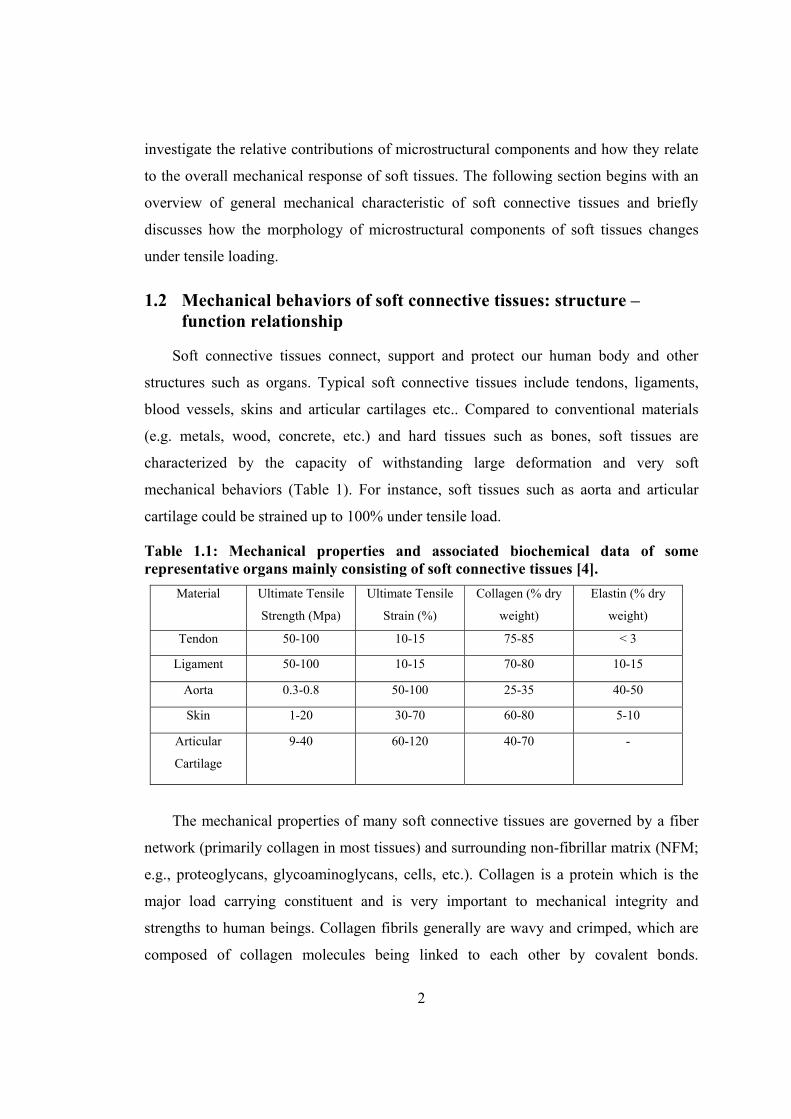
Table 1.1: Mechanical properties and associated biochemical data of some representative organs mainly consisting of soft connective tissues [4].

Material Ultimate Tensile

Strength (Mpa)

Ultimate Tensile

Strain (%)

Collagen (% dry

weight)

Elastin (% dry

weight)

Tendon 50-100 10-15 75-85 < 3

Ligament 50-100 10-15 70-80 10-15

Aorta 0.3-0.8 50-100 25-35 40-50

Skin 1-20 30-70 60-80 5-10

Articular

Cartilage

9-40 60-120 40-70 -

The mechanical properties of many soft connective tissues are governed by a fiber

network (primarily collagen in most tissues) and surrounding non-fibrillar matrix (NFM;

e.g., proteoglycans, glycoaminoglycans, cells, etc.). Collagen is a protein which is the

major load carrying constituent and is very important to mechanical integrity and

strengths to human beings. Collagen fibrils generally are wavy and crimped, which are

composed of collagen molecules being linked to each other by covalent bonds.

3

Depending on the primary function and strength requirement of soft tissues, the diameter

of individual fibrils varies. Also, the arrangement of collagen fibrils is different from

tissue to tissue. For tendon and ligament which are primarily loaded in tension, the

structure of their collagen fibrils appears as parallel oriented fibers to maximum the load

bearing capacity. Another example is intervertebral discs, where fibers of the annulus

fibrosus are oriented in multiple directions to be able to adapt to the multiple loading

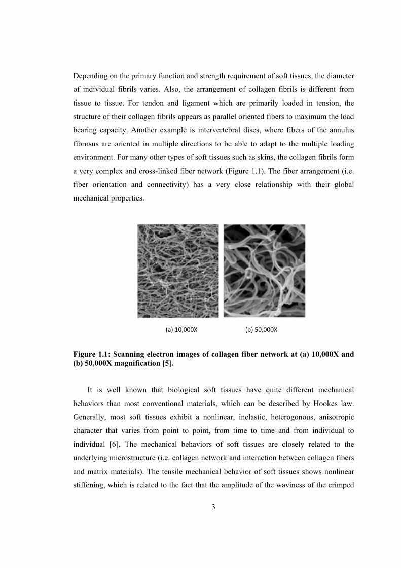
environment. For many other types of soft tissues such as skins, the collagen fibrils form

a very complex and cross-linked fiber network (Figure 1.1). The fiber arrangement (i.e.

fiber orientation and connectivity) has a very close relationship with their global

mechanical properties.

(a) 10,000X (b) 50,000X

Figure 1.1: Scanning electron images of collagen fiber network at (a) 10,000X and (b) 50,000X magnification [5].

It is well known that biological soft tissues have quite different mechanical

behaviors than most conventional materials, which can be described by Hookes law.

Generally, most soft tissues exhibit a nonlinear, inelastic, heterogonous, anisotropic

character that varies from point to point, from time to time and from individual to

individual [6]. The mechanical behaviors of soft tissues are closely related to the

underlying microstructure (i.e. collagen network and interaction between collagen fibers

and matrix materials). The tensile mechanical behavior of soft tissues shows nonlinear

stiffening, which is related to the fact that the amplitude of the waviness of the crimped

4

fibers decreases at initial strain region and fiber reorientation to the load direction. Also,

some tissues show viscous behavior (relaxation and creep), which are known to be

associated with the viscous interaction between collagen fibrils and the matrix of

proteoglycans.

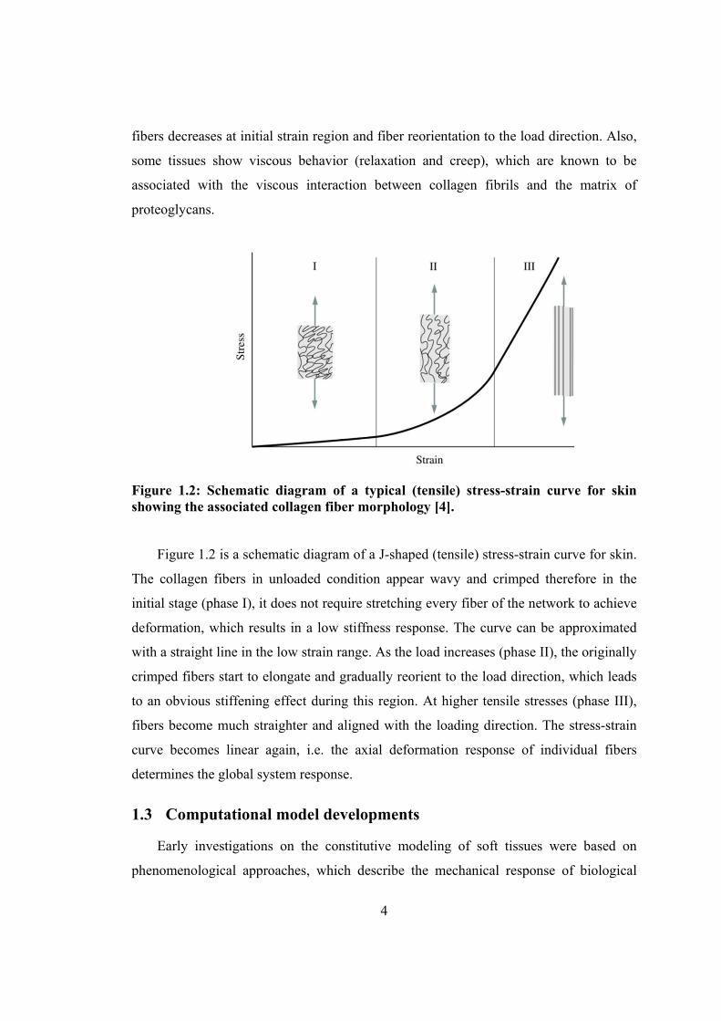
Figure 1.2: Schematic diagram of a typical (tensile) stress-strain curve for skin showing the associated collagen fiber morphology [4].

Figure 1.2 is a schematic diagram of a J-shaped (tensile) stress-strain curve for skin.

The collagen fibers in unloaded condition appear wavy and crimped therefore in the

initial stage (phase I), it does not require stretching every fiber of the network to achieve

deformation, which results in a low stiffness response. The curve can be approximated

with a straight line in the low strain range. As the load increases (phase II), the originally

crimped fibers start to elongate and gradually reorient to the load direction, which leads

to an obvious stiffening effect during this region. At higher tensile stresses (phase III),

fibers become much straighter and aligned with the loading direction. The stress-strain

curve becomes linear again, i.e. the axial deformation response of individual fibers

determines the global system response.

1.3 Computational model developments

Early investigations on the constitutive modeling of soft tissues were based on

phenomenological approaches, which describe the mechanical response of biological

5

materials under applied load by fitting a mathematic equation to the observed stress-

strain curves of tissue specimens. Based on experimental elongation results on rabbits’

mesentery, Fung [7] developed a one dimensional constitutive model for simple

elongation where the tensile stress is an exponential form function of strain. Later, he

expanded the one-dimensional model to 3D by postulating an existence of a three

dimensional pseudostrain energy function 1 , which led to an exponential

relationship between second Piola-Kirchhoff stress tensor and the Green strain tensor.

There are other forms of strain energy functions proposed to describe mechanical

behavior of various types of soft tissues. Early forms of strain energy function W

borrowed ideas from the field of rubber elasticity because both rubberlike material and

soft tissue are composed of similar long-chained, cross-linked polymeric

microstructures. In such a framework, the strain energy function W is related to

deformation by W=W(IC,IIC) in various forms, where IC=tr(C), IIC=(tr(C))2 – tr(C2) are

coordinate invariant measures of the right Cauchy strain tensor C [6]. However, the

disadvantage of such methods is that they are not able to capture the anisotropic

behavior generally exhibited by biological materials. Later Humphrey [8] proposed a

new form of pseudostrain-energy function W for transversely isotropic biomaterials such

as myocardium. In his study, the strain energy function takes the following form:

W=W(IC, IVC) where IC=tr(C) and IVC=M·C·M, with M denoting a measure of fiber

orientation in such material obtained from a biaxial stretching test.

Although phenomenological models [7, 8, 9, 10] provided initial insights into the

mechanics of fibrillar tissues, the disadvantage of such models is that it is unable to

reveal the underlying mechanism that determines the mechanical behavior at functional

scale. Hence, structural models [11, 12, 13, 14, 15, 16, 17, 18, 19] which include

collagen fibers explicitly modeled as one of the components, have emerged to capture

more information about the tissue architecture and they have been applied to a variety of

intact tissues and tissue components such as lung, collagen, cartilage, mature skin.

In the work of Lanir et al. [11], the tissue total strain energy is assumed to be the

sum of individual fiber strain energies transformed from individual fiber (local)

coordinates to tissue (global) coordinates. This model allows the use of fiber orientation

distribution information (experimental values or mathematic function) and individual

6

fiber constitutive models to formulate the tissue stress-strain relationship and is based on

the affine deformation assumption. Based on Lanir’s model, several researchers have

successfully applied and refined the model to predict the mechanical behavior of a

variety of tissues [13, 20, 21]. In order to directly incorporate quantitative structural

information for direct implementation, Sacks [13] directly incorporated the fiber

orientation distribution parameter obtained by using small angle light scattering (SALS)

in the constitutive model formulation. And it was demonstrated that this model

accurately predicted the measured biaxial mechanical response of native bovine

pericardium by only requiring a single equibiaxial test to determine the effective fiber

stress-strain response and the SALS-derived fiber orientation distribution. In order to

capture the accurate stress-strain response of arterial layers, a general hyper-elastic free

energy function was developed in by Gasser et al. [21] with explicit representation of the

dispersion of collagen fiber orientation in the adventitial and intimal layers, as shown by

polarized light microscopy of strained arterial tissue. In particular, by using continuous

fiber angular distribution in articular cartilage matrix modeling, Ateshian [20] was able

to predict the transition of very low Poisson’s ratio (~0.02) in compression to very high

values in tension (~2), which could not be explained by previous models with only three

orthogonal fiber bundles to describe the tissue matrix.

Another approach adopted generalized structure tensors (GST) to model tissues with

continuous distributed collagen fibers [22]. These tensors are used to represent the three-

dimensional distribution of fibers. The strain of individual fiber is assumed affine and

obtained as the multiplication of structure tensor and the global strain tensor. Compared

to the approach based on continuous fiber orientation distribution, this approach is

relatively simple and requires a smaller amount of calculations to get the fiber strain

energy and stress. However, as pointed out in [14], this approach can only be used when

fibers are all in tension and the angular distribution is small.

In the aforementioned literature, there is a key assumption that individual collagen

fibers are acting independently (i.e. without interaction with other fibers) and deform

according to the macroscopic deformation field, which is popularly known as the ‘affine’

model. However, these models perform poorly when applied to networks with low

density or networks subjected to complex loading paths [23]. Nonaffine deformation is

7

widely observed in experimental studies [24, 25]. In order to investigate the effect of

network nonaffinity (NA) on the overall mechanical behavior of soft tissues, full

network models composed of interconnected fibers allowing for fiber-fiber interaction

have been developed. Fiber crosslinks are modeled as pin-joints [26] or rotation joints

(pin joint transmits no moments and fiber only carries axial force; however, rotation

joint allows bending of fibers) [27, 28, 29]. The degree of non-affinity is determined by

network density, individual fiber constitutive properties and also the observation scale.

Chandran [26] compared the affine-model and the network model and it was shown that

the network behavior was actually characterized by extensive fiber reorientation and

moderate stretch ratios, which in turn gives a softer mechanical response of the network

on the system level than affine approaches. Onck [30] indicated that strain-stiffening

observed in semi-flexible networks (e.g. cytoskeleton) is caused by nonaffine network

arrangement, which governs a transition from bending-dominated response at small

strain to stretching dominated response at large strains. They also indicated that filament

undulations merely postpone the transition. Liu [31] measured the local strain field for a

semi-flexible network under shear and observed that the degree of nonaffinity increases

with the decrease of crosslink density.

Various measures have been used to quantify the degree of nonaffinity [29, 30, 32,

33]. A strain-based measure was introduced in [29] by Hatami-Marbini and Picu to

probe the network mechanics at various scales. The degree of NA decreases as the length

scale of observation increases and the scaling is a power law with different exponents for

length scales smaller or larger than a characteristic length scale proportional to the fiber

length. It was also found that as bending stiffness of fibers increases relative to axial

stiffness, the NA decreases. Onck [30] employed a nonaffine (NA) measure ||δu-uaff||

(where u is the actual displacement of crosslinks and uaff is the corresponding affine

displacement) and showed that the degree of NA decreases when the network is

subjected to large deformations.

The mechanical interaction between collagen fiber network and the nonfibrillar

matrix is also being studied. Nonfibrillar matrix is often modeled using a simple

mathematical representation, such as Neo-Hookean [34, 35, 36, 37] or Mooney-Rivlin

[38, 39, 40, 41] and is assumed to contribute to the fiber-matrix composite in a summed

8

or ‘parallel’ sense. For instance, in the study on mechanical modeling of arterial wall

conducted by Holzapfel [34], the isochoric strain energy function Ψ of the two layered

fiber reinforced composite was considered to be the summation of two parts, Ψiso

associated with the mechanical response of non-matrix material and Ψaniso associated

with the anisotropic mechanical behavior of collagen fibers. Similarly, in Tang et al.

[36], the contribution of matrix material was accounted for by an additional strain energy

in neo-hookean form weighted by the volume ratio of the matrix material. Some other

models [42, 43, 44] have utilized an additional term to account for the fiber-matrix

interaction. However, in general, the appropriate definition for the interaction term is

unknown. To overcome this limitation, the current study presents a method wherein the

collagen fiber network and surrounding NFM are microscopically coupled, making it

possible to evaluate specifically the interaction between fibers and matrix.

1.4 Organization of dissertation

Chapter 2 discusses the pre-processing step for the coupled fiber-matrix model. In

order to use automatic meshing to create fiber-matrix finite element model, non-

manifold geometric representation is employed. Then it introduces the non-manifold

geometric creation for the fiber embedded matrix and specifies the topological

adjacencies between topological entities that make up the geometric model. Next the

multi-dimensional mesh generation is described to derive both the isotropic and graded

meshes from the created geometry.

Chapter 3 presents the nonlinear finite element formulations for the coupled fiber-

matrix system. Both geometric and material nonlinearities are taken into account in the

nonlinear finite element analysis. Tangential stiffness matrix and force vector are

derived for the coupled fiber-matrix system. Standard Newton’s iteration is employed to

solve the nonlinear equations.

Chapter 4 analyzes the finite element results of the uniaxial extension by employing

the coupled fiber-matrix model. The overall constitutive response of the coupled fiber-

matrix system is compared with the parallel model for the same set of input parameters;

Interactions between the two constituents are investigated by examining the stress

distribution of the matrix material and the nonaffine measure of network deformation;

9

An analytical method is proposed to predict the effective elastic modulus and Poisson’s

ratio of the RVE composite.

Chapter 5 presents a volume averaging based multiscale model to effectively link

the microstructure mechanics to the overall tissue mechanics. By applying the multiscale

approach, fiber reorientation occurring in the tissue microstructure is captured in the

dogbone uniaxial extension test.

Chapter 6 concludes the present work and describes possible future improvements.

10

2. Non-manifold geometry modeling and mesh generation

2.1 Introduction and overview of the coupled model

Microstructural modeling is essential to characterize and quantify the roles of

collagen and non-fibrillar matrix (NFM) in imparting mechanical properties to soft

tissues at functional level. Recently, a computational network-based microstructural

model (referred here as parallel model) was developed by our collaborators to examine

how specific NFM properties alter the response of fiber-matrix composites under load

[45]. This model is constructed according to the conventional “parallel” approach of

superposition of the two constituents (i.e., collagen network and NFM). Some relevant

details of the parallel model are provided here for clarity. In the parallel model, the stress

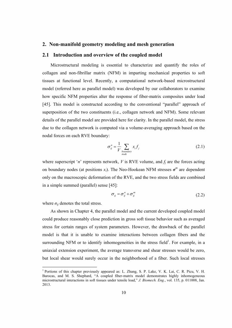
due to the collagen network is computed via a volume-averaging approach based on the

nodal forces on each RVE boundary:

1n

ij i jboundarynode

x fV

(2.1)

where superscript ‘n’ represents network, V is RVE volume, and fj are the forces acting

on boundary nodes (at positions xi). The Neo-Hookean NFM stresses σm are dependent

only on the macroscopic deformation of the RVE, and the two stress fields are combined

in a simple summed (parallel) sense [45]:

n mij ij ij (2.2)

where σij denotes the total stress.

As shown in Chapter 4, the parallel model and the current developed coupled model

could produce reasonably close prediction in gross soft tissue behavior such as averaged

stress for certain ranges of system parameters. However, the drawback of the parallel

model is that it is unable to examine interactions between collagen fibers and the

surrounding NFM or to identify inhomogeneities in the stress field1. For example, in a

uniaxial extension experiment, the average transverse and shear stresses would be zero,

but local shear would surely occur in the neighborhood of a fiber. Such local stresses

1 Portions of this chapter previously appeared as: L. Zhang, S. P. Lake, V. K. Lai, C. R. Picu, V. H. Barocas, and M. S. Shephard, “A coupled fiber-matrix model demonstrates highly inhomogeneous microstructural interactions in soft tissues under tensile load,” J. Biomech. Eng., vol. 135, p. 011008, Jan. 2013.

11

could be much larger than average values, which could have important implications in

initiating failure of the NFM or in greatly altering the site-specific cellular environment.

Therefore, a fully coupled fiber network and matrix model is developed in present study,

which is capable of (a) quantifying local stresses throughout the computational domain

and (b) exploring interactions between NFM and the embedded collagen network. The

coupled model can also be used in the future to study material failure driven by fiber or

matrix damage accumulation.

Both the parallel model and the current coupled fiber-matrix model are based on a

full fiber network representation with direct account for interactions between individual

fibers, which can be modeled as three-dimensional cylinders or simplified one-

dimensional structural elements (i.e., truss or beam). However, it has been shown that

explicit representation of the volume of fibers is not necessary when volume fraction

occupied by fibers is small [46]. Furthermore, in the coupled fiber-matrix model, the

matrix prevents the fibers from coming in direct contact with each other during

deformation at points other that the existing cross links, so representing the fiber volume

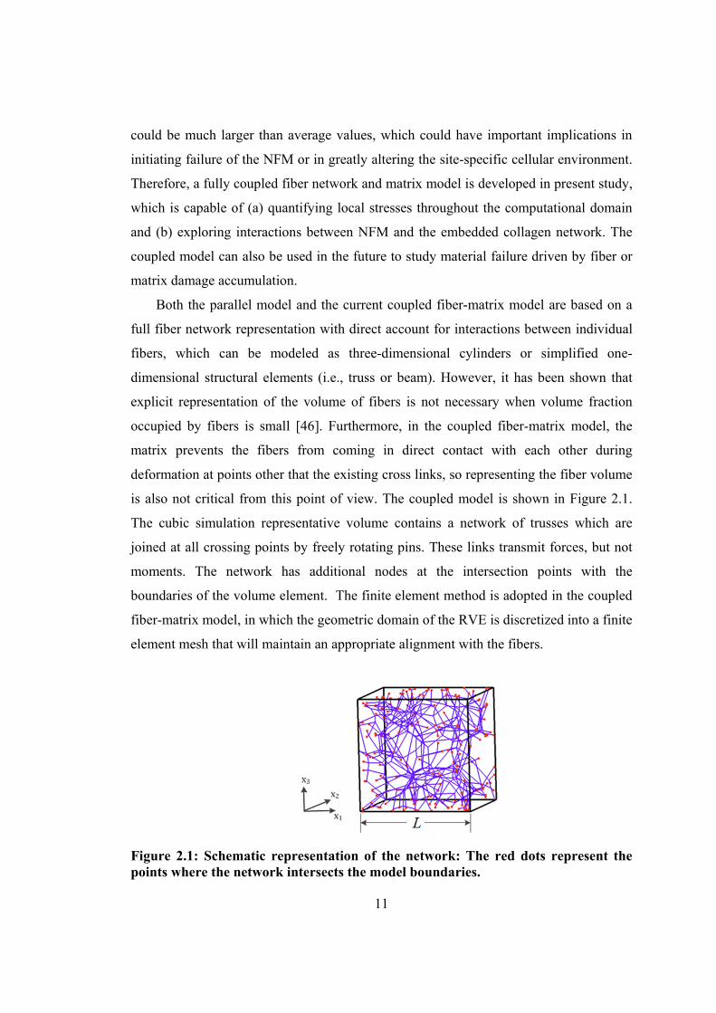
is also not critical from this point of view. The coupled model is shown in Figure 2.1.

The cubic simulation representative volume contains a network of trusses which are

joined at all crossing points by freely rotating pins. These links transmit forces, but not

moments. The network has additional nodes at the intersection points with the

boundaries of the volume element. The finite element method is adopted in the coupled

fiber-matrix model, in which the geometric domain of the RVE is discretized into a finite

element mesh that will maintain an appropriate alignment with the fibers.

Figure 2.1: Schematic representation of the network: The red dots represent the points where the network intersects the model boundaries.

12

The workflow for applying the finite element method (see Figure 2.2) includes four

steps: (1) Creation of a fiber network; (2) creation of the geometric model represented in

non-manifold form based on the generated fiber network; (3) multidimensional mesh

generation from the created geometry; and (4) formulation and solution of finite element

equations of the coupled fiber and matrix system.

Figure 2.2: Work-flow demonstrating construction protocol for the coupled model.

This chapter presents the methods used for the first three steps, which are Voronoi

fiber network generation (section 2.2), non-manifold geometry creation of fiber

embedded matrix (section 2.3) and multi-dimensional mesh generation (section 2.4).

Chapter 3 presents the finite element formulation of the fiber network with matrix.

2.2 Voronoi fiber network generation

Voronoi networks are used to represent the locations of fibers in the unit cell in the

present study due to their ability to provide a close approximation to collagen gel

behavior [47]. Such networks exhibit very large Poisson’s ratios (~3) similar to those

observed experimentally due to its low coordination number compared to other types of

model networks [5]. This section overviews the process of Voronoi fiber network

generation, the output of which is used as input for generating the geometry of fiber

network within a matrix material.

The procedure of Voronoi network generation is shown in Figure 2.3 and

summarized as follows [45]:

Step 1: Seed points are randomly placed in a cubic box with side length L.

13

Step 2: The Voronoi tessellation is formed around the generated seed points.

Step 3: The edges of the Voronoi cells become network segments.

Step 4: Nodes are placed at edge intersections and at intersections with the cube

boundaries.

Step 1. Random seed points Step 2. Voronoi Tessellation

Step 3. Fiber Network Step 4. Nodes at intersections of fibers

and between fibers and boundaries

Figure 2.3: Procedure of Voronoi network generation.

14

Note that in this model fibers do not carry cross-links in the middle of the fiber

span. There are only two cross-links per fiber and these are placed at the ends of the

respective fiber where it either intersects other fibers or the RVE boundary. The

generated network contains two essential components of information, which completely

defines the network configuration:

(1) Fiber connectivity defining which fiber is adjacent to which fiber crosslinks;

(2) Spatial coordinates of crosslinks.

The following are the input parameters used to characterize the generated Voronoi

networks:

Network density , defined as the total length of fibers per unit volume:

3

N

ii

l

L

(2.3)

where N is the total number of fibers, li is i-th fiber length and L is the side length of the

unit cube.

Mean segment length lc:

N

ii

c

ll

N

(2.4)

Fiber orientation parameter:

2 2 21 2 3

11 22 33

/ / /, ,

N N N

i i i i i ii i i

N N N

i i ii i i

l l l l l l

l l l

(2.5)

where l1i , l2i and l3i are the projections of fiber length in x1, x2 and x3 directions

respectively. For an isotropic network, 11 22 33 1/ 3 ; for a perfectly aligned

network in x1 direction, 11 1 [48].

These network parameters play an important role in determining the overall network

behavior as shown in [23, 26, 29, 48]. The result analysis presented in Chapter 4 uses

these parameters to identify different random networks.

15

2.3 Non-manifold geometric modeling using Parasolid

The geometric model contains topological and shape information of the object being

analyzed. In the current study, the geometry of fiber network within solid matrix is

created based on a full representation of the embedded fiber network, i.e. the

connectivity of the fibers and spatial coordinates of fiber crosslinks are explicitly

represented and could be queried by CAD modelers. Since each individual embedded

fiber is considered as one-dimensional geometric edge, which has zero cross-section

area, conventional manifold modeling is not able to properly represent the desired

model. Instead, non-manifold form, which provides a much more general geometric

representation, is adopted in the current geometric modeling.

2.3.1 Introduction to non-manifold and manifold models

Compared to manifold solid presentation, non-manifold form is able to provide a

unified representation of general combinations of 1-D, 2-D and 3-D geometric entities.

A manifold (more strictly stated 2-manifold) solid representation is one where every

point on a surface is two dimensional, which means that every point on the boundary has

a boundary neighborhood which is homeomorphic to a two-dimensional disk [49].

However, non-manifold geometric models do not maintain this constraint. In other

words, the surface area around a given point need not be a simple two-dimensional disk.

Hence, in such a framework, it allows non-manifold situations such as a cone touching

upon another surface at a single point, wire edges embedded in solid volume or

emanating from a point on a surface, or more than two faces meeting along a common

edge. These situations are common to engineering analysis idealizations and it greatly

increases the efficiency and productivity in engineering practices if one could account

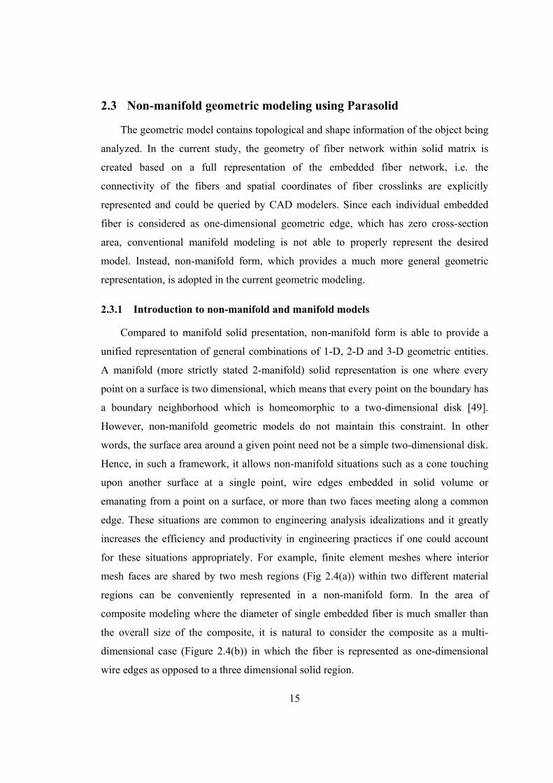
for these situations appropriately. For example, finite element meshes where interior

mesh faces are shared by two mesh regions (Fig 2.4(a)) within two different material

regions can be conveniently represented in a non-manifold form. In the area of

composite modeling where the diameter of single embedded fiber is much smaller than

the overall size of the composite, it is natural to consider the composite as a multi-

dimensional case (Figure 2.4(b)) in which the fiber is represented as one-dimensional

wire edges as opposed to a three dimensional solid region.

16

Figure 2.4: (a) Cellular body: Interior face shared by two regions – each side of the face is used by the associated region; (b) Multi-dimensional body: Three-dimensional region with embedded one-dimensional wire edges.

2.3.2 General description of construction of the non-manifold geometric model

The Parasolid geometric modeling kernel [50] is employed to construct the non-

manifold geometric representation of the fiber-matrix model. This section uses the same

terminology as used in Parasolid.

Following the definition of a geometry, which is topology with attached geometric

information, the process of creating the non-manifold fiber-matrix model is therefore

conducted in two steps: the first is to construct the topology by specifying topological

entities that make up the model and describing adjacent relationships between these

entities; Once the topology is constructed, the geometric information defining the shape

of that entity is attached to associated topological entities. A description of topology and

geometric entities is provided first; then the non-manifold topological adjacencies of the

specific case-multi-dimensional fiber-matrix model are discussed.

Topology and topological entities

Topology serves as the structure or skeleton of a geometric model. It consists of

topological entities that are linked through a set of adjacent relationships.

Types of topological entities include:

Body

A body could be considered as a repository for all topological entities from zero to three

dimensions.

17

Region

A region is a connected volume of space whose boundary is a collection of shells.

Regions could be either solid or void (empty). A body always has an infinite void region,

which could be considered as all the space outside the body itself.

Shell

In a manifold representation, a shell is a connected set of faces (each used by shell on

one side of the face) which form a closed volume. However, in a non-manifold

representation, the definition of a shell is much more general, which could be a

combination of adjacent faces, a wireframe or even a single vertex.

Face

A face is a bounded portion of a shell. Its boundary is a collection of zero or more loops.

An example of zero loop is a spherical surface.

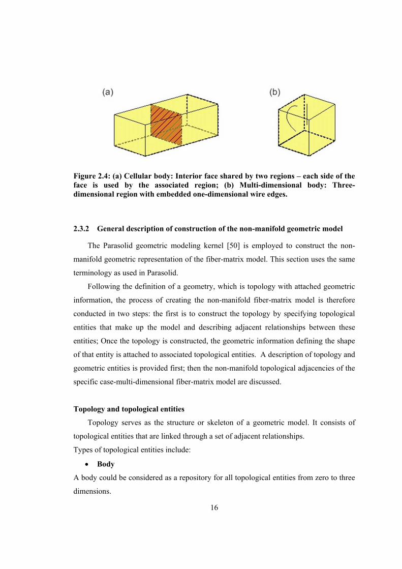
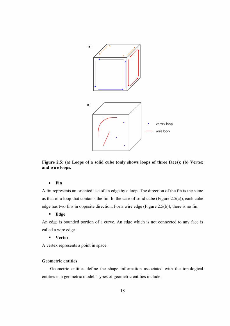
Loop

A loop is a connected boundary of a single face. It consists of an oriented sequence of

edges (Figure 2.5(a)) or may be just a single vertex loop or wire loop (Figure

2.5(b)).Vertex or wire loops are corresponding to vertices or edges scribed inside a face.

Fiber crosslinks on the RVE boundaries are represented as vertex loops.

18

vertex loop

wire loop

Figure 2.5: (a) Loops of a solid cube (only shows loops of three faces); (b) Vertex and wire loops.

Fin

A fin represents an oriented use of an edge by a loop. The direction of the fin is the same

as that of a loop that contains the fin. In the case of solid cube (Figure 2.5(a)), each cube

edge has two fins in opposite direction. For a wire edge (Figure 2.5(b)), there is no fin.

Edge

An edge is bounded portion of a curve. An edge which is not connected to any face is

called a wire edge.

Vertex

A vertex represents a point in space.

Geometric entities

Geometric entities define the shape information associated with the topological

entities in a geometric model. Types of geometric entities include:

19

Surfaces are attached to faces of the model.

Curves are attached to edges or fins of the model.

Points are attached to vertices. All points are Cartesian points.

2.3.3 Constructing the non-manifold model of fiber and matrix

The non-manifold topological adjacencies for the geometry of fibers within matrix

are discussed based on the rules of non-manifold geometric model construction. To

make the description clearer, a case with three embedded fibers (Figure 2.6) in solid

matrix is used as an example.

Figure 2.6: Three fibers within matrix – blue lines and blue dots represent embedded fibers and fiber crosslinks (only one inner crosslink, the other three are boundary crosslinks); black lines and black dots represent cube edges and cube vertices.

The geometry in Figure 2.6 contains the following topologies entities:

Body: there is only one body which serves as a container to hold all topological

entities.

Regions: an infinite void region and a solid region.

Shells: two shells here. A shell enclosing the void region and a shell associated with

the solid region. The shell enclosing the solid region consists of cube faces (inner side of

cube faces is used by the solid region) and embedded three wire edges representing

fibers.

20

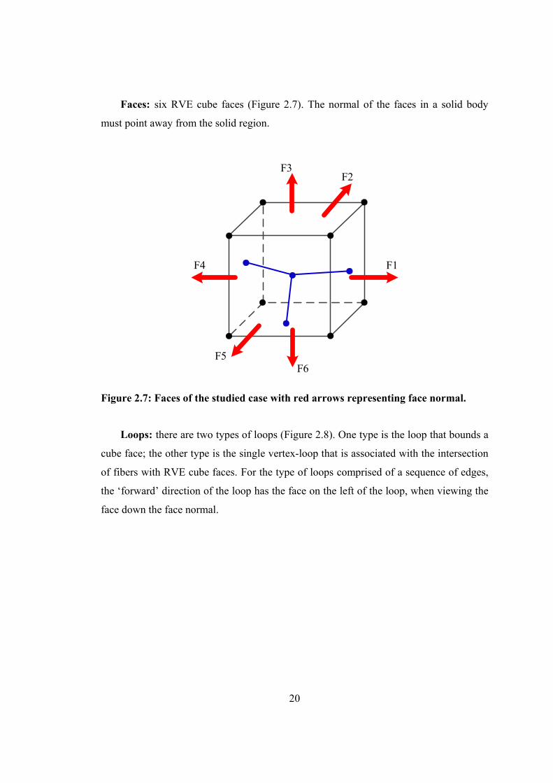
Faces: six RVE cube faces (Figure 2.7). The normal of the faces in a solid body

must point away from the solid region.

F1

F2F3

F4

F5F6

Figure 2.7: Faces of the studied case with red arrows representing face normal.

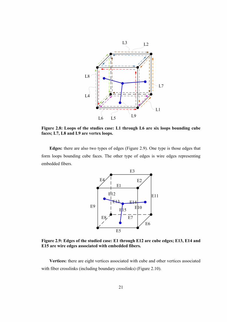
Loops: there are two types of loops (Figure 2.8). One type is the loop that bounds a

cube face; the other type is the single vertex-loop that is associated with the intersection

of fibers with RVE cube faces. For the type of loops comprised of a sequence of edges,

the ‘forward’ direction of the loop has the face on the left of the loop, when viewing the

face down the face normal.

21

L3

L1

L2

L4

L5L6

L7

L8

L9

Figure 2.8: Loops of the studies case: L1 through L6 are six loops bounding cube faces; L7, L8 and L9 are vertex loops.

Edges: there are also two types of edges (Figure 2.9). One type is those edges that

form loops bounding cube faces. The other type of edges is wire edges representing

embedded fibers.

E1E2

E3

E4

E5

E6

E7E8

E9 E10

E11E12

E13 E14

E15

Figure 2.9: Edges of the studied case: E1 through E12 are cube edges; E13, E14 and E15 are wire edges associated with embedded fibers.

Vertices: there are eight vertices associated with cube and other vertices associated

with fiber crosslinks (including boundary crosslinks) (Figure 2.10).

22

V1 V2

V3V4

V5 V6

V7V8

V9V10 V11

V12

Figure 2.10: Vertices of the studied case: V1 through V8 are cube vertices; V9, V10, V11 and V12 are vertices associated with fiber crosslinks in which V10 is an embedded vertex.

To create a topology using Parasolid, it is required to specify all topological

adjacencies between topological entities existing in the model one would want to

generate. Following terminology in Parasolid, each topological adjacent relationship is

defined by three entries: parent, child and sense; ‘Parent’ and ‘Child’ refer to two

adjacent topological entities; ‘Sense’ indicates the manner in which a child is used by its

parent. In relationships in which ‘sense’ matters, ‘sense’ should be set to ‘positive’ or

‘negative’; In relationships in which ‘sense’ does not matter, it should be set to ‘none’.

Table 2.1 to 2.8 list topological adjacent relationships between each topological entity

described in section 2.3.3. When using Parasolid to create topology, these listed

topological adjacent relationships need to be specified.

Table 2.1: Body ~ Region adjacent relationships.

Parents Children Senses

Body R_void negative

Body R_solid positive

‘Negative’ means the region is void; ‘Positive’ means the region is solid.

23

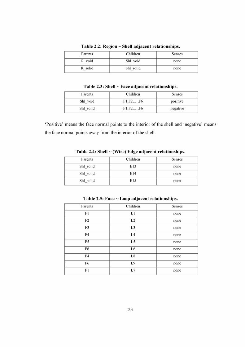
Table 2.2: Region ~ Shell adjacent relationships.


R_void Shl_void none

R_solid Shl_solid none

Table 2.3: Shell ~ Face adjacent relationships.


Shl_void F1,F2,…,F6 positive

Shl_solid F1,F2,…,F6 negative

‘Positive’ means the face normal points to the interior of the shell and ‘negative’ means

the face normal points away from the interior of the shell.

Table 2.4: Shell ~ (Wire) Edge adjacent relationships.


Shl_solid E13 none

Shl_solid E14 none

Shl_solid E15 none

Table 2.5: Face ~ Loop adjacent relationships.


F1 L1 none

F2 L2 none

F3 L3 none

F4 L4 none

F5 L5 none

F6 L6 none

F4 L8 none

F6 L9 none

F1 L7 none

24

Table 2.6: Loop ~ Edge adjacent relationships.


L1 E6 positive

L1 E11 positive

L1 E2 positive

L1 E10 positive

L2 E7 positive

L2 E11 negative

L2 E3 positive

L2 E12 positive

L3 E1 positive

L3 E2 negative

L3 E3 negative

L3 E4 positive

L4 E4 negative

L4 E12 negative

L4 E8 positive

L4 E9 positive

L5 E1 negative

L5 E9 negative

L5 E5 positive

L5 E10 negative

L6 E5 negative

L6 E6 negative

L7 E7 negative

L8 E8 negative

‘Positive’ means the edge is in the same direction of as the loop; ‘negative’ means the

edge is in the opposite direction to the loop.

Table 2.7: Loop ~ Vertex adjacent relationships.


L7 V11 none

L8 V9 none

L9 V12 none

25

Table 2.8: Edge ~ Vertex adjacent relationships.


E1 V1,V2 none

E2 V2,V3 none

E3 V3,V4 none

E4 V4,V1 none

E5 V5,V6 none

E6 V6,V7 none

E7 V7,V8 none

E8 V8,V5 none

E9 V1,V5 none

E10 V2,V6 none

E11 V3,V7 none

E12 V4,V8 none

E13 V9,V10 none

E14 V10,V11 none

E15 V10,V12 none

2.4 Multi-dimensional mesh generation

Once the geometry of fiber network within matrix is created, the next step is to load

the geometry into mesh generator to create an appropriate mesh. In the present study,

Simmetrix Inc. meshing tools [51] are used to create the conforming mesh from the

generated geometry. The generated mesh is multi-dimensional with 3D tetrahedrons for

the solid matrix and 1D truss elements for the collagen fibers. The solid matrix and

embedded fiber network are meshed together such that mesh vertices and mesh edges on

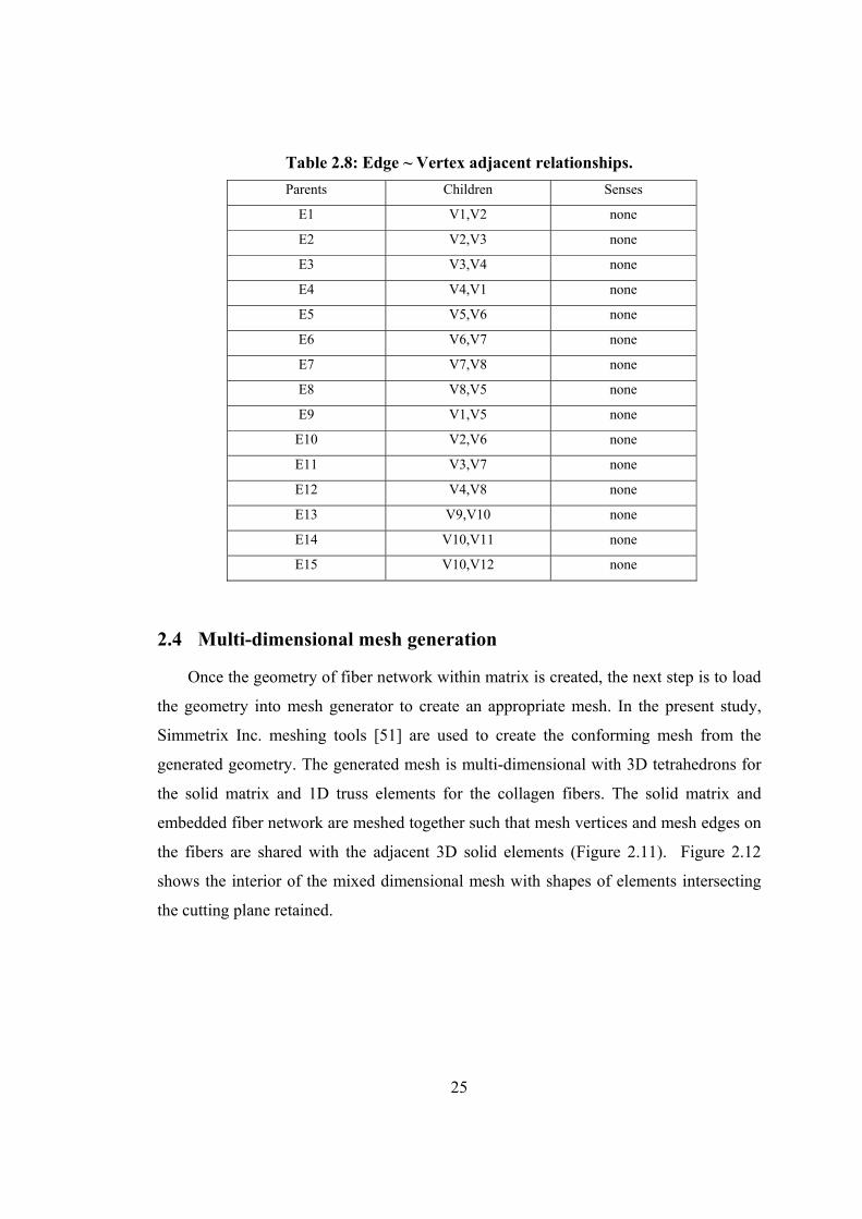
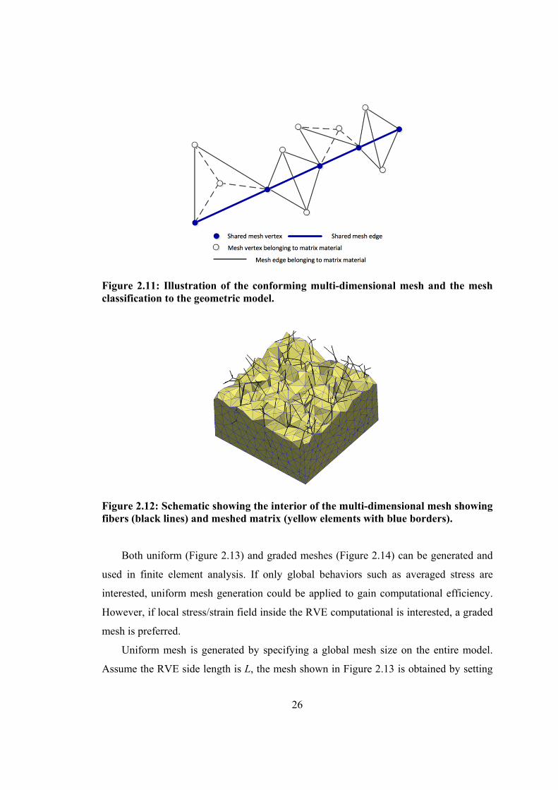
the fibers are shared with the adjacent 3D solid elements (Figure 2.11). Figure 2.12

shows the interior of the mixed dimensional mesh with shapes of elements intersecting

the cutting plane retained.

26

Figure 2.11: Illustration of the conforming multi-dimensional mesh and the mesh classification to the geometric model.

Figure 2.12: Schematic showing the interior of the multi-dimensional mesh showing fibers (black lines) and meshed matrix (yellow elements with blue borders).

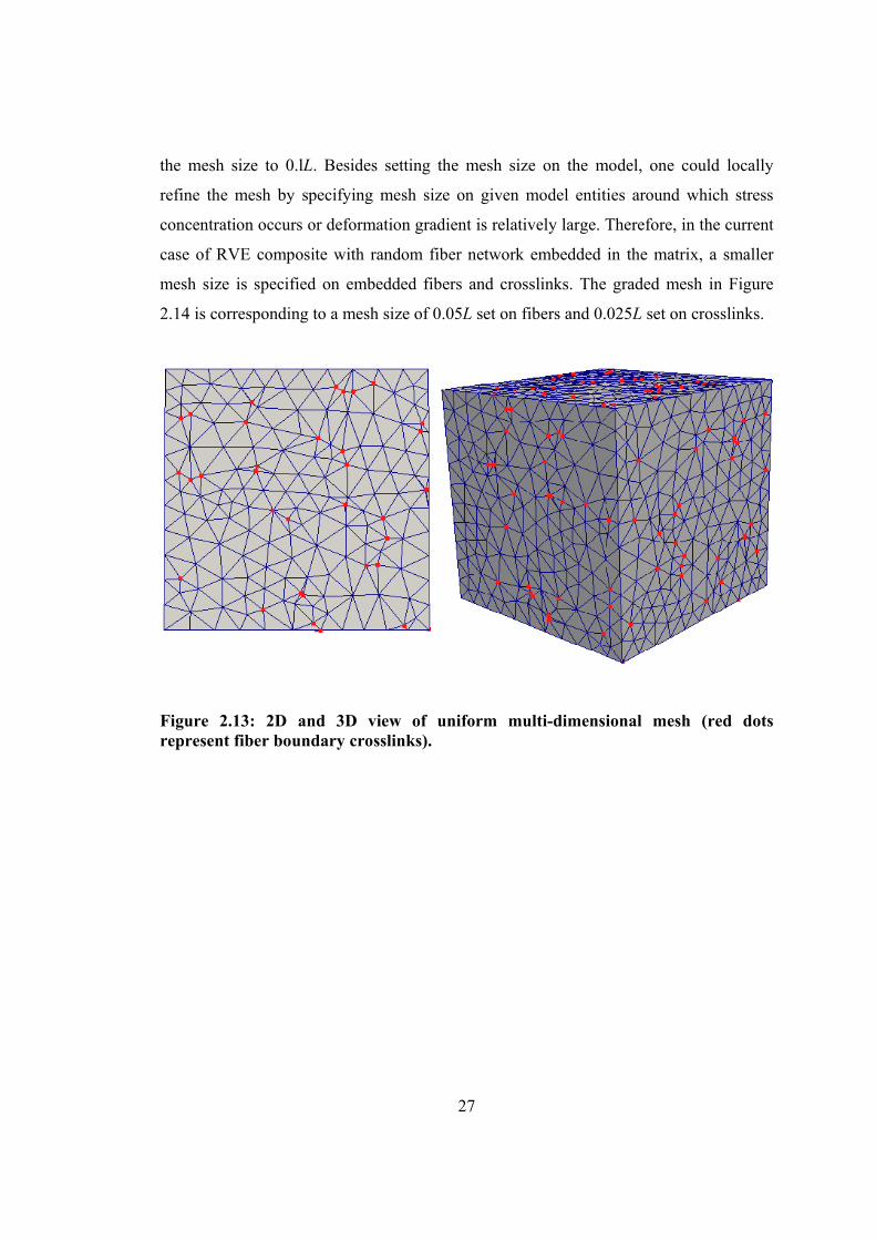
Both uniform (Figure 2.13) and graded meshes (Figure 2.14) can be generated and

used in finite element analysis. If only global behaviors such as averaged stress are

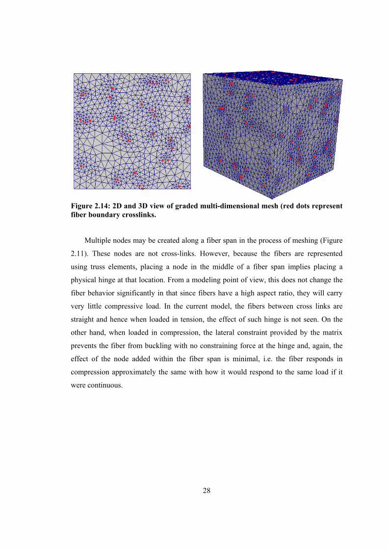
interested, uniform mesh generation could be applied to gain computational efficiency.

However, if local stress/strain field inside the RVE computational is interested, a graded

mesh is preferred.

Uniform mesh is generated by specifying a global mesh size on the entire model.

Assume the RVE side length is L, the mesh shown in Figure 2.13 is obtained by setting

27

the mesh size to 0.lL. Besides setting the mesh size on the model, one could locally

refine the mesh by specifying mesh size on given model entities around which stress

concentration occurs or deformation gradient is relatively large. Therefore, in the current

case of RVE composite with random fiber network embedded in the matrix, a smaller

mesh size is specified on embedded fibers and crosslinks. The graded mesh in Figure

2.14 is corresponding to a mesh size of 0.05L set on fibers and 0.025L set on crosslinks.

Figure 2.13: 2D and 3D view of uniform multi-dimensional mesh (red dots represent fiber boundary crosslinks).

28

Figure 2.14: 2D and 3D view of graded multi-dimensional mesh (red dots represent fiber boundary crosslinks.

Multiple nodes may be created along a fiber span in the process of meshing (Figure

2.11). These nodes are not cross-links. However, because the fibers are represented

using truss elements, placing a node in the middle of a fiber span implies placing a

physical hinge at that location. From a modeling point of view, this does not change the

fiber behavior significantly in that since fibers have a high aspect ratio, they will carry

very little compressive load. In the current model, the fibers between cross links are

straight and hence when loaded in tension, the effect of such hinge is not seen. On the

other hand, when loaded in compression, the lateral constraint provided by the matrix

prevents the fiber from buckling with no constraining force at the hinge and, again, the

effect of the node added within the fiber span is minimal, i.e. the fiber responds in

compression approximately the same with how it would respond to the same load if it

were continuous.

29

3. Finite element analysis of the coupled fiber-matrix model

In this chapter the nonlinear finite element equations needed to predict the

mechanical behavior of the coupled fiber-matrix system are presented. The source of

nonlinearity of the current study comes from material nonlinearity and geometric

nonlinearity (large deformations). The material models adopted for representing

embedded fibers and matrix materials are presented in section 3.1. Section 3.2 presents

the nonlinear finite element equations formulated for 3D linear tetrahedrons and 1D truss

members while section 3.3 presents the assembling process with coupled tetrahedrons

and truss members.

3.1 Material model representing embedded fiber and matrix

Collagen fibers are represented as one-dimensional nonlinear members with

constitutive behavior defined as [45, 52]:

( 1)ffib BE Af e

B (3.1)

where ffib is the axial force in a given fiber, Ef is the fiber Yong’s modulus in the zero-

strain limit, A is the fiber cross-sectional area, B is a nonlinearity constant and ε is the

fiber Green’s strain along the fiber, defined as 0.5 1 where is the fiber

stretch ratio. Eq. (3.1) specifies properties for individual fibers; of course the mechanical

response of each RVE result from the collective behavior of the full network of fibers.

The present study uses the same value of material parameters as in [52]:

EfA=0.0065827N, B=3.8.

The non-fibrillar matrix (NFM) is represented as a compressible neo-Hookean solid,

with the second Piola Kirchhoff stress tensor S defined as [53]:

1

3 mG GI S I C (3.2)

where Gm is the NFM shear modulus, I is the identity matrix, I3=λ1λ2λ3, λ1,λ2,λ3 are

eigenvalues of C, which is the right Cauchy deformation tensor, / (1 2 )m m , and

νm is Poisson’s ratio of the NFM. As done previously [45], νm is set to 0.1. The NFM

shear modulus is varied over a range of values (Gm = 10, 110, 720 and 4300 Pa)

corresponding to 0.05, 0.125, 0.25 and 0.5 % w/v (weight of the solute in volume)

30

agarose in our experimental collagen-agarose studies [5]. To assess the role of

compressibility, a set of simulations with low compressibility of νm =0.45 is also

evaluated for Gm=110 Pa.

As discussed in section 3.2, the formation of the tangent stiffness matrix requires

evaluation of the material tangent elasticity tensor (fourth order) ˆijrsC defined as

ˆ / , , , , 1, 2,3ijrs ij rsC S i j r s (3.3)

where ɛrsis the Green strain tensor.

With the NFM modeled as neo-hookean Eq.(3.2), the material tangent elasticity ˆijrsC is

expressed as [53]:

1 1 1 11 2

ˆ C C C C C (3.4a)

1 3 2 32 , 2GI GI (3.4b)

1 1 1 1( )ijkl ij klC C C C (3.4c)

1 1 1 1 1 11( )

2 ik jl il jkijklC C C C C C (3.4d)

3.2 Nonlinear finite element formulation of the coupled fiber-matrix model

In a linear analysis, it is assumed that the displacements of the body under

consideration are infinitesimally small and that the material is linear elastic. With these

assumptions, there is no need to differentiate between initial (undeformed) and current

(deformed) configuration and therefore engineering stress and strain are appropriately

employed to formulate the equilibrium equations. However, when the body exhibits

large deformations, the equilibrium equations need to be established in the current

configuration.

In practice, the calculation of the finite element solution is carried out in a step by

step manner instead of applying the external load all together to ensure that the nonlinear

iteration converges. In a nonlinear analysis, the aim is to evaluate the equilibrium state

of the body at the discrete load points 0, Δt , 2Δt, 3Δt, …, where Δt represents the load

increment. In the following section, it is assumed that solutions of static and kinematic

31

variables for all load steps from 0, Δt , 2 Δt, …, have all been calculated. The task is to

seek the unknown state corresponding to load level at t + Δt. A standard Newton-

Raphson iterative approach [54, 55] is adopted here to solve the nonlinear finite element

equations. The iterative procedure is described in Section 3.2.1; the derivation of the

linearized finite element equations including tangential stiffness matrix and residual

force vector with respect to linear tetrahedrons and truss members is presented in

subsequent sections.

3.2.1 Newton-Raphson iterative approach

The equilibrium state of a system of finite elements representing the problem

domain corresponding to load level t + Δt is expressed as

( )t t t t t tint ext f u f (3.5)

where t t

intf and

t textf

are internal (‘int’) and external (‘ext’) nodal force vectors and

ut+∆t is the nodal displacement vector at equilibrium state of load level t+ Δt.

Using Taylor’s series and assuming ( )t t t t

i u u u

where ( )

t tiu is the nodal

displacement vector at iteration i, the internal nodal force vector t t

intf is expanded as

( )

( )

( )( ) ( )

t tt t t t t t t t int

int int i

i

f uf u f u u

u (3.6)

Substituting the above equation into Eq.(3.5),

( )

( )

( )( )

t tt t t t t tint

ext int i

i

f uu f f u

u (3.7)

Let ( )

( )

( )t tint

i

i

f u

Ku

, which is the tangential stiffness matrix at iteration i.

Hence, Eq.(3.7) is written as

( ) ( )( )t t t t t ti ext int i res

K u f f u f

(3.8)

where ( )( )t t t t t text int i f f u

is the residual force vector, denoted as fres.

Solving the linear system defined by Eq.(3.8) to obtain u , which is then used to

update the nodal displacement vector at iteration i+1 ( 1)t tiu , i.e.

32

( 1) ( )t t t ti i u u u

(3.9)

The above iterative process continues until the norm of fres is smaller than a predefined

convergence tolerance. The L2-norm of fres is employed in the current study.

3.2.2 Nonlinear finite element equations

In the case of finite deformation, it must be ensured the that stress and strain

measures employed to formulate the nonlinear finite element equations are work

conjugate pairs [54, 56]. In the present study, the second Piola-Kirchhoff stress tensor Sij

and the Green-Lagrange strain tensor ɛij are taken to be the stress and strain measures,

respectively. As the basis for deriving the displacement based finite element formulation,

the principle of virtual displacement established in the current (unknown) configuration

is written as

0

0t t t t t t

ij ij

V

S dV R

(3.10)

The superscript t+Δt represents the configuration in which the quantity (stress,

strain, body force, surface traction, etc.) occurs, i.e. t tijS and t t

ij denote second

Piola-Kirchhoff stress and Green strain measured at the unknown configuration

corresponding to load level at t+Δt; t tR is the virtual external work induced by the

virtual displacement applied at the unknown configuration at load level t+Δt.

The first step to derive the linearized finite element formulation is to write the

principle of virtual displacement at t+Δt (Eq.(3.10) ) as an incremental decomposition,

i.e. to express the virtual internal work (left hand side of Eq.(3.10)) by use of known

quantities at t and associated increments from t to t+Δt.

t t t

ij ij ijS S S

(3.11a)

t t t

ij ij ij

(3.11b)

where ijS and ij are incremental stress and strain from load level t to t+ Δt;

By definition of Green strain [57],

, , , ,

1( ) , 1, 2,3

2t t t t t t t t t t

ij i j j i k i k ju u u u i j

(3.12a)

33

, , , ,

1( ) , 1, 2,3

2t t t t t

ij i j j i k i k ju u u u i j (3.12b)

where ui,j is the derivative of the ith component of displacement with respect to the jth

component of spatial coordinates. Subtracting Eq.(3.12b) from Eq.(3.12a) and using

, 1,2,3t t ti i iu u u i , the incremental Green’s strain ij is obtained as

, , , , , , , ,

1 1( )

2 2t t t t t

ij ij ij i j j i k i k j k j k i k i k ju u u u u u u u (3.13)

Further decomposing the incremental Green’s strain ij into two terms, ije

and ij ,

ij ij ije

(3.14a)

, , , , , ,

1( )

2t t

ij i j j i k i k j k j k ie u u u u u u

(3.14b)

, ,

1

2ij k i k ju u

(3.14c)

in which ije is linear with iu (note that ,

tk iu

is a known quantity) and ij

is

nonlinear with iu . It is shown in the next section that these two terms contribute to the

linear and nonlinear part of tangential stiffness matrix, respectively.

Substituting the above incremental forms of stress and strain (Eq.3.11, 3.14) into

Eq.(3.10) and noting that ( )t t tij ij ij ij , the principle of virtual

displacement with incremental decomposition is obtained

0 0 0

0 0 0t t t t

ij ij ij ij ij ij

V V V

S dV S dV R S e dV

(3.15)

Linearizing the first term on the left hand side using a Taylor series,

0 0

0 0( h.o.t.) ( )ijij ij rs ij ij

rsV V t

SS dV e dV

(3.16a)

Neglecting higher order terms (h.o.t) in the Taylor series and using rs rs rse ,

Eq.(3.16a) becomes

34

0 0

0

0 0( ) ( )

( )

ijij ij rs rs ij ij

rsV V t

ijrs ij rs ij rs ij rs ij

rsV t

SS dV e e dV

Se e e e

(3.16b)

Noting that , , , ,

1( )

2ij k i k j k j k iu u u u and , ,

1

2ij k i k ju u , hence, among

the four terms in the bracket in Eq. (3.16b), only the first term rs ije e is linear with

incremental displacement iu and the left three terms are higher order terms which are

neglected. Eq. (3.16b) becomes

0 0 0

0 0 0ij

ij ij rs ij ijrs rs ijrsV V Vt

SS dV e e dV C e e dV

(3.17)

where

ijijrs

rs t

SC

is the fourth order material tangent elasticity tensor evaluated at known

configuration corresponding to load step at t.

Substituting Eq.(3.17) into Eq.(3.15), the following equation is constructed

0 0 0

0 0 0t t t t

ijrs rs ij ij ij ij ij

V V V

C e e dV S dV R S e dV (3.18)

which is the principle of virtual displacements after linearization. From Eq. (3.18), the

linear tangent matrix stiffness LK , nonlinear tangent matrix stiffness NLK are derived.

To make Eq.(3.18) more compact, each term in the equation can be case in a matrix

format

0

0 0

0 0 0ˆ ˆ( )

TT T

ijrs rs ij L LVV V

C e e dV dV dV e C e u B CB Δu

(3.19a)

0

0 0

0 0 0( )Tt T t T t

ij ij NL NLVV V

S dV dV dV η S η u B S B Δu (3.19b)

0

0 0

0 0 0ˆ ˆ( )

Tt T t T tij ij LV

V V

S e dV dV dV e S u B S

(3.19c)

35

0 0 0

0 0 0ˆ ˆT T t t t T t

V V V

dV dV R dV e C e η S η e S (3.19d)

where

11 22 33 12 23 31[ 2 2 2 ]Te e e e e e e

1,1 1,2 1,3 2 ,1 2 ,2 2,3 3,1 3,2 3,3

Tu u u u u u u u u η

1111 1122 1133 1112 1123 1131

2211 2222 2233 2212 2223 2231

3311 3322 3333 3312 3323 3331

1211 1222 1233 1212 1223 1231

2311 2322 2333 2333 2323 2323

3111 3122 3133 3133 3123 3123

ˆ

C C C C C C

C C C C C C

C C C C C C

C C C C C C

C C C C C C

C C C C C C

C

,

11 12 13

12 22 23

13 23 33

0 0 0

, , 0 0 0

0 0 0

t t t

t t t t

t t t

S S S

S S S

S S S

S 0 0

S 0 S 0 S 0

0 0 S

11 22 33 12 23 13ˆ Tt t t t t t tS S S S S S S

By interpolating the displacement field with appropriate shape functions, the

incremental strain vectors eand η are related to nodal displacement vector u by

L e B u and NL η B u , where

LB and N LB are correspondingly linear and

nonlinear strain-displacement matrix respectively. Hence, Eq.(3.19d) is written as

0 0

0

0 0

0

ˆ( ) ( )

ˆ( )

T TT T tL L NL NLV V

Tt t T tLV

dV dV

R dV

u B CB Δu u B S B Δu

u B S

(3.20)

Assuming there is no external force ( 0t tR ),

0 0

0

0 0

0

ˆ( ) ( )

ˆ( )

T TT T tL L NL NLV V

TT tLV

dV dV

dV

u B CB Δu u B S B Δu

u B S

(3.21)

The above equation is valid for arbitrary virtual incremental displacement u , by

eliminating u

0 0 00 0 0

ˆ ˆT T Tt tL L NL NL LV V V

dV dV dV B CB Δu B S B Δu B S

(3.22)

36

Let

00

T

L L LVdV K B CB

(3.23a)

0

T tNL NL NLV

dV K B S B

(3.23b)

00

ˆT tLV

dV f B S

(3.23c)

Therefore

( )L NL K K u f (3.24)

3.2.3 Strain-displacement relationship for three dimensional matrix elements

This section derives the linear and nonlinear strain-displacement matrices BL and

BNL by interpolating the displacement field using shape functions.

The displacement field of the linear tetrahedral element representing matrix material

is interpolated by linear shape functions 1 2 3 4T N N N NN , i.e.

4

1

ki k i

k

u N u

, i=1,2,3 (3.25)

where kiu is the ith component of displacement vector at node k.

(1) Linear strain-displacement matrix BL ( L e B u )

Recall

11 22 33 12 23 31

, , , , , ,

[ 2 2 2 ]

1( ), , , 1, 2,3

2

T

t tij i j j i k i k j k j k i

e e e e e e

e u u u u u u i j k

e

and write

0 1

0 1, L L L e e e B B B (3.26a)

0 1

0 1,L L e B u e B u (3.26b)

where 0 0 0 0 0 0 0

11 22 33 12 23 31[ 2 2 2 ]Te e e e e e e

1 1 1 1 1 1 111 22 33 12 23 31[ 2 2 2 ]Te e e e e e e

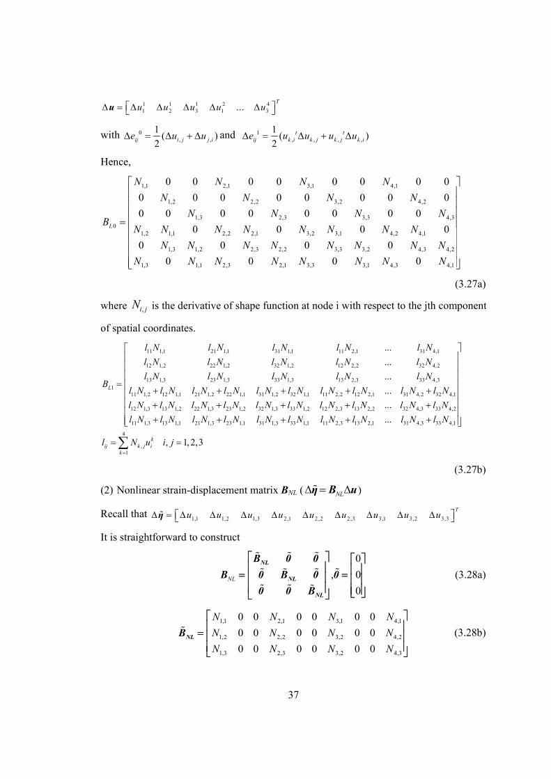
37

1 1 1 2 41 2 3 1 3...

Tu u u u u u

with 0, ,

1( )

2ij i j j ie u u and 1, , , ,

1( )

2t t

ij k i k j k j k ie u u u u

Hence,

1,1 2,1 3,1 4,1

1,2 2,2 3,2 4,2

1,3 2,3 3,3 4,30

1,2 1,1 2,2 2,1 3,2 3,1 4,2 4,1

1,3 1,2 2,3 2,2 3,3 3,2 4,3 4,2

1,3 1,1 2,3 2,1 3,3 3,1 4,3 4,1

0 0 0 0 0 0 0 0

0 0 0 0 0 0 0 0

0 0 0 0 0 0 0 0

0 0 0 0

0 0 0 0

0 0 0 0

L

N N N N

N N N N

N N N NB

N N N N N N N N

N N N N N N N N

N N N N N N N N

(3.27a)

where ,i jN is the derivative of shape function at node i with respect to the jth component

of spatial coordinates.

11 1,1 21 1,1 31 1,1 11 2,1 31 4,1

12 1,2 22 1,2 32 1,2 12 2,2 32 4,2

13 1,3 23 1,3 33 1,3 13 2,3 33 4,31

11 1,2 12 1,1 21 1,2 22 1,1 31 1,2 32 1,1 11 2,2 12 2,1 31 4,2 32 4,1

12

...

...

...

...L

l N l N l N l N l N

l N l N l N l N l N

l N l N l N l N l NB

l N l N l N l N l N l N l N l N l N l N

l N

1,3 13 1,2 22 1,3 23 1,2 32 1,3 33 1,2 12 2,3 13 2,2 32 4,3 33 4,2

11 1,3 13 1,1 21 1,3 23 1,1 31 1,3 33 1,1 11 2,3 13 2,1 31 4,3 33 4,1

4

,1

...

...

, 1, 2,3kij k j i

k

l N l N l N l N l N l N l N l N l N

l N l N l N l N l N l N l N l N l N l N

l N u i j

(3.27b)

(2) Nonlinear strain-displacement matrix BNL ( NL η B u)

Recall that 1,1 1,2 1,3 2 ,1 2 ,2 2,3 3,1 3,2 3,3

Tu u u u u u u u u η

It is straightforward to construct

0

, 0

0NL

NL

NL

NL

B 0 0

B 0 B 0 0

0 0 B

(3.28a)

1,1 2,1 3,1 4,1

1,2 2,2 3,2 4,2

1,3 2,3 3,2 4,3

0 0 0 0 0 0

0 0 0 0 0 0

0 0 0 0 0 0

N N N N

N N N N

N N N NNLB

(3.28b)

38

3.2.4 Nonlinear finite element formulation for one dimensional truss element

The nonlinear equations for one dimensional truss elements (Figure 3.1) are derived

in a more straightforward manner since the expression of nodal forces at two ends of the

truss element can be easily obtained by projecting axial force along the spatial axis. The

element tangent stiffness matrix TRK is obtained by direct differentiation of the element

nodal force vector f with respect the nodal displacement vector u [54], i.e.

TR f

Ku

(3.29)

where

1 1 1 1 1 11 1 1 1 1 11 1 1 2 2 21 2 3 1 2 3

1 1 1 1 1 12 2 2 2 2 21 1 1 2 2 21 2 3 1 2 3

1 1 1 1 1 13 3 3 3 3 31 1 1 2 2 21 2 3 1 2 3

2 2 2 2 2 21 1 1 1 1 11 1 1 2 2 21 2 3 1 2 3

22

TR

f f f f f f

u u u u u u

f f f f f f

u u u u u u

f f f f f f

u u u u u u

f f f f f f

u u u u u u

f

K

2 2 2 2 22 2 2 2 2

1 1 1 2 2 21 2 3 1 2 3

2 2 2 2 2 23 3 3 3 3 31 1 1 2 2 21 2 3 1 2 3

f f f f f

u u u u u u

f f f f f f

u u u u u u

element nodal force vector f

1 1 1 2 2 2

1 2 3 1 2 3

Tf f f f f ff

(3.30)

1 1 1 2 2 21 2 3 1 2 3

Tu u u u u u u (3.31)

where j

if is the ith component of nodal force vector at node j and j

iu is the ith component

of displacement vector at node j.

By projecting the fiber axial force ffib along spatial axis, the element nodal force vector

f is written as

1 2 2 11 2 1 2 2 1 2 13 3 3 31 1 2 2 1 1 2 2[ ]fib Tx x x xx x x x x x x x

fl l l l l l

f

(3.32)

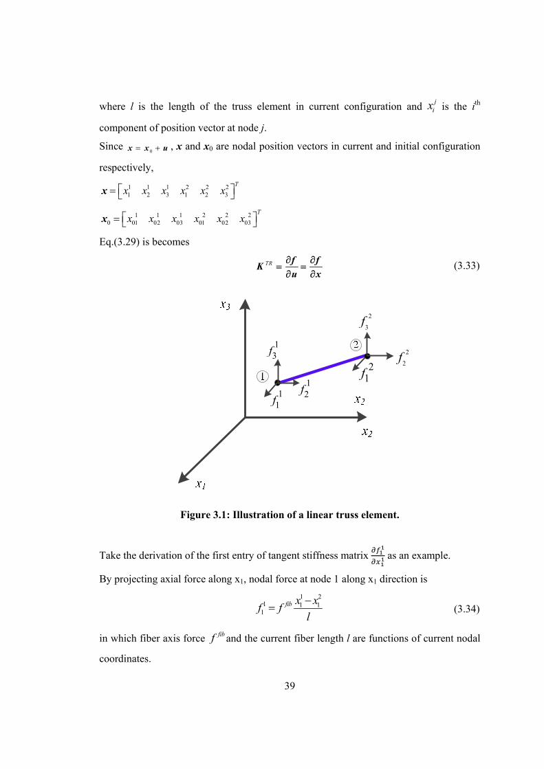
39

where l is the length of the truss element in current configuration and j

ix is the ith

component of position vector at node j.

Since 0 x x u , x and x0 are nodal position vectors in current and initial configuration

respectively,

1 1 1 2 2 21 2 3 1 2 3

Tx x x x x x x

1 1 1 2 2 20 01 02 03 01 02 03

Tx x x x x x x

Eq.(3.29) is becomes

TR f f

Ku x

(3.33)

11f

12f

13f

21f

2

2f

2

3f

Figure 3.1: Illustration of a linear truss element.

Take the derivation of the first entry of tangent stiffness matrix as an example.

By projecting axial force along x1, nodal force at node 1 along x1 direction is

1 21 1 1

1fib x x

f fl

(3.34)

in which fiber axis force fibf and the current fiber length l are functions of current nodal

coordinates.

40

Using the chain rule,

1 1 11 1 11 1 11 1 1

fib fib

fib

f f ff l l f

x f l x l x l

(3.35)

The first two terms of the right hand side of Eq.(3.35) are written as:

21 1 21 1 1

11

fib fib

fib

f x xf l f

f l x l l

(3.36)

21 1 21 1 1

11

fibf x xl f

l x l l

(3.37)

Hence,

21 1 21 1 111

fib fib fibf x xf f f

x l l l l

(3.38a)

Similarly,

1 1 2 1 21 1 1 2 212

fib fibf x x x xf f

x l l l l

(3.38b)

1 21 1 23 31 1 1

13

fib fib x xf x xf f

x l l l l

(3.38c)

1 1 1 1 1 11 1 1 1 1 12 1 2 1 2 11 1 2 2 3 3

, ,f f f f f f

x x x x x x

(3.38d)

1 1 2 1 2 12 1 1 2 2 11 11 2

fib fibf x x x x ff f

x l l l l x

(3.38e)

21 1 22 2 212


x l l l l

(3.38f)

1 21 1 23 32 2 2

13

fib fib x xf x xf f

x l l l l

(3.38g)

1 1 1 1 1 12 2 2 2 2 22 1 2 1 2 11 1 2 2 3 3

, ,f f f f f f

x x x x x x

(3.38h)

1 1 21 2 13 3 31 1 11 11 3

fib fibf x xx x ff f

x l l l l x

(3.38i)

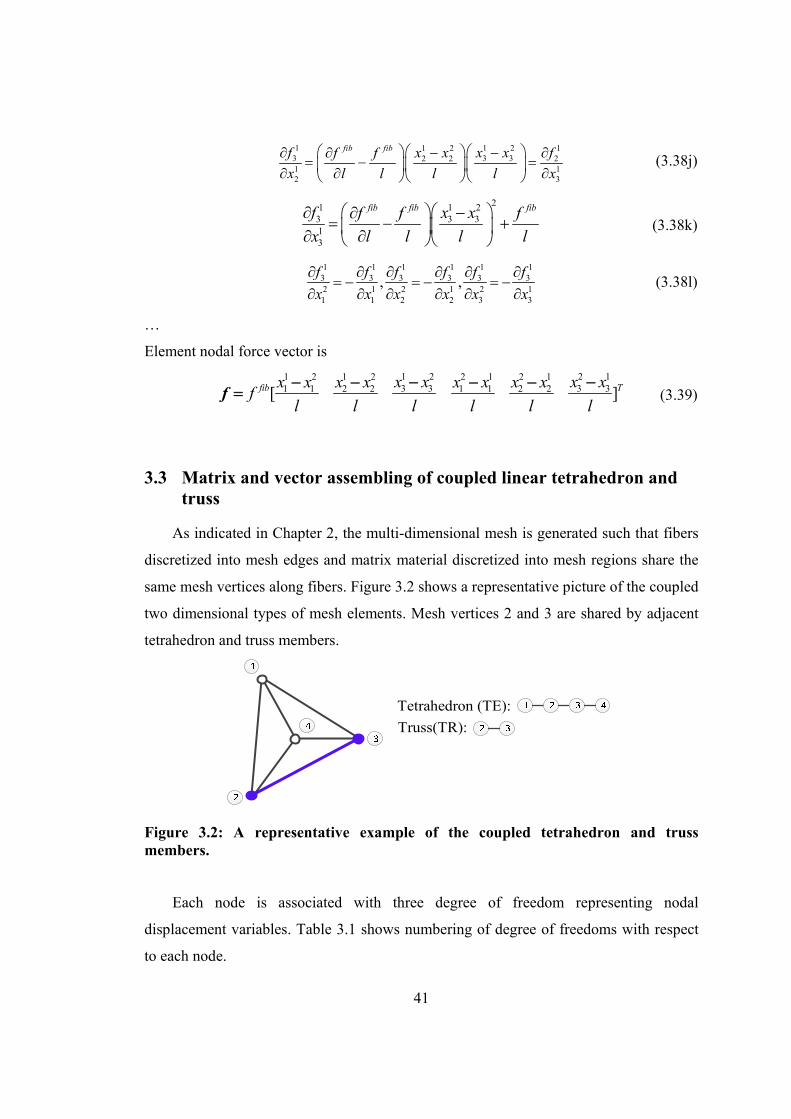
41

1 1 21 2 13 3 32 2 21 12 3

fib fibf x xx x ff f

x l l l l x

(3.38j)

21 1 23 3 313


x l l l l

(3.38k)

1 1 1 1 1 13 3 3 3 3 32 1 2 1 2 11 1 2 2 3 3

, ,f f f f f f

x x x x x x

(3.38l)

…

Element nodal force vector is

1 2 2 11 2 1 2 2 1 2 13 3 3 31 1 2 2 1 1 2 2[ ]fib Tx x x xx x x x x x x x

fl l l l l l

f

(3.39)

3.3 Matrix and vector assembling of coupled linear tetrahedron and truss

As indicated in Chapter 2, the multi-dimensional mesh is generated such that fibers

discretized into mesh edges and matrix material discretized into mesh regions share the

same mesh vertices along fibers. Figure 3.2 shows a representative picture of the coupled

two dimensional types of mesh elements. Mesh vertices 2 and 3 are shared by adjacent

tetrahedron and truss members.

Tetrahedron (TE):

Truss(TR):

Figure 3.2: A representative example of the coupled tetrahedron and truss members.

Each node is associated with three degree of freedom representing nodal

displacement variables. Table 3.1 shows numbering of degree of freedoms with respect

to each node.

42

Table 3.1: Numbering of degree of freedoms

Node Number Numbering of Degree of

freedom

1 1,2,3

2 4,5,6

3 7,8,9

4 10,11,12

For the example shown in Figure 3.2, the element tangential stiffness matrix from

tetrahedron (‘TE’) TEeK is written as

1 4 5 9 121 1 1 1 11 4 5 9 122 2 2 2 21 4 5 9 123 3 3 3 31 4 5 9 124 4 4 4 41 4 5 9 125 5 5 5 51 4 5 9 126 6 6 6 61 4 5 9 127 7 7 7 71 4 5 98 8 8 8

... ... ...

... ... ...

... ... ...

... ... ...

... ... ...

... ... ...

... ... ...

... ... ..

TEe

p p p p p

p p p p p

p p p p p

p p p p p

p p p p p

p p p p p

p p p p p

p p p p

K

128

1 4 5 9 129 9 9 9 91 4 5 9 1210 10 10 10 101 4 5 9 1211 11 11 11 111 4 5 9 1212 12 12 12 12 12 12

.

... ... ...

... ... ...

... ... ...

... ... ...

p

p p p p p

p p p p p

p p p p p

p p p p p

(3.40)

in which the entry ijp represents it is located in row j (which is associated with degree j)

and column i (which is associated with degree i) in the global system. The element

tangential matrix stiffness from truss (‘TR’) TReK is written as

43

4 5 6 7 8 94 4 4 4 4 44 5 6 7 8 95 5 5 5 5 54 5 6 7 8 96 6 6 6 6 64 5 6 7 8 97 7 7 7 7 74 5 6 7 8 98 8 8 8 8 84 5 6 7 8 99 9 9 9 9 9 6 6

TRe

q q q q q q

q q q q q q

q q q q q q

q q q q q q

q q q q q q

q q q q q q

K

(3.41)

When assembling TEeK and

TReK together, the entries with the same locations in the

global system is added together to form the global stiffness matrix cpK ,

1 4 5 9 121 1 1 1 11 4 5 9 122 2 2 2 21 4 5 9 123 3 3 3 31 4 4 5 5 9 9 124 4 4 4 4 4 4 41 4 4 5 5 9 9 125 5 5 5 5 5 5 51 4 4 5 5 9 9 126 6 6 6 6 6 6 61 47 7

... ... ...

... ... ...

... ... ...

... ... ...

... ... ...

... ... ...

...cp

p p p p p

p p p p p

p p p p p

p p q p q p q p

p p q p q p q p

p p q p q p q p

p p

K4 5 5 9 9 127 7 7 7 7 7

1 4 4 5 5 9 9 128 8 8 8 8 8 8 81 4 4 5 5 9 9 129 9 9 9 9 9 9 91 4 5 9 1210 10 10 10 101 4 5 9 1211 11 11 11 111 4 5 9 1212 12 12 12 12

... ...

... ... ...

... ... ...

... ... ...

... ... ...

... ... ...

q p q p q p

p p q p q p q p

p p q p q p q p

p p p p p

p p p p p

p p p p p

12 12

(3.42)

Similar assembling process is done with the tetrahedron element force vector and

truss element force vector to obtain the global force vector.

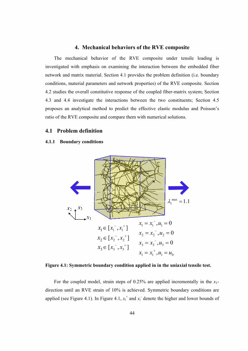
44

4. Mechanical behaviors of the RVE composite

The mechanical behavior of the RVE composite under tensile loading is

investigated with emphasis on examining the interaction between the embedded fiber

network and matrix material. Section 4.1 provides the problem definition (i.e. boundary

conditions, material parameters and network properties) of the RVE composite. Section

4.2 studies the overall constitutive response of the coupled fiber-matrix system; Section

4.3 and 4.4 investigate the interactions between the two constituents; Section 4.5

proposes an analytical method to predict the effective elastic modulus and Poisson’s

ratio of the RVE composite and compare them with numerical solutions.

4.1 Problem definition

4.1.1 Boundary conditions

1 11 [ , ]x xx

2 22 [ , ]x xx

3 33 [ , ]x xx

1 1 1

2 2 2

3 3 3

1 1 1 0

, 0

, 0

, 0

,

x x u

x x u

x x u

x x u u

max1 1.1

Figure 4.1: Symmetric boundary condition applied in in the uniaxial tensile test.

For the coupled model, strain steps of 0.25% are applied incrementally in the x1-

direction until an RVE strain of 10% is achieved. Symmetric boundary conditions are

applied (see Figure 4.1). In Figure 4.1, xi+ and xi

- denote the higher and lower bounds of

45

the RVE cube in i-direction (i=1, 2, 3); ui is the displacement in i-direction(i=1, 2, 3); u0

is the applied displacement boundary condition to the surface perpendicular to x1

direction and λ1max is the maximum stretch ratio applied at the RVE cube along x1

direction. Other faces perpendicular to x2 and x3 axes are kept traction free.

4.1.2 Nomenclature

To effectively present the results, table 4.1 summarizes the notations of parameters

used in this chapter. The definitions of some parameters are also referenced.

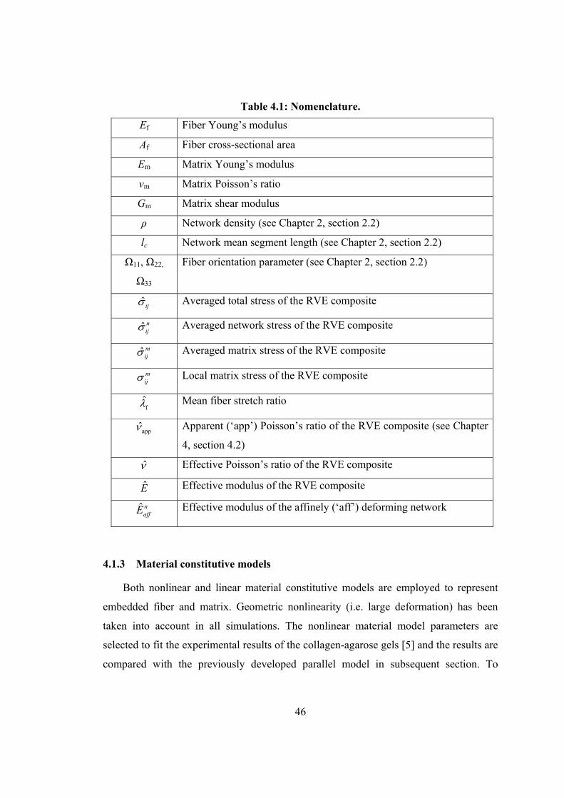
46

Table 4.1: Nomenclature.

Ef Fiber Young’s modulus

Af Fiber cross-sectional area

Em Matrix Young’s modulus

νm Matrix Poisson’s ratio

Gm Matrix shear modulus

ρ Network density (see Chapter 2, section 2.2)

lc Network mean segment length (see Chapter 2, section 2.2)

Ω11, Ω22,

Ω33

Fiber orientation parameter (see Chapter 2, section 2.2)

ˆij Averaged total stress of the RVE composite

ˆ nij Averaged network stress of the RVE composite

ˆ mij Averaged matrix stress of the RVE composite

mij Local matrix stress of the RVE composite

f Mean fiber stretch ratio

app Apparent (‘app’) Poisson’s ratio of the RVE composite (see Chapter

4, section 4.2)

Effective Poisson’s ratio of the RVE composite

E Effective modulus of the RVE composite

ˆ naffE Effective modulus of the affinely (‘aff’) deforming network

4.1.3 Material constitutive models

Both nonlinear and linear material constitutive models are employed to represent

embedded fiber and matrix. Geometric nonlinearity (i.e. large deformation) has been

taken into account in all simulations. The nonlinear material model parameters are

selected to fit the experimental results of the collagen-agarose gels [5] and the results are

compared with the previously developed parallel model in subsequent section. To

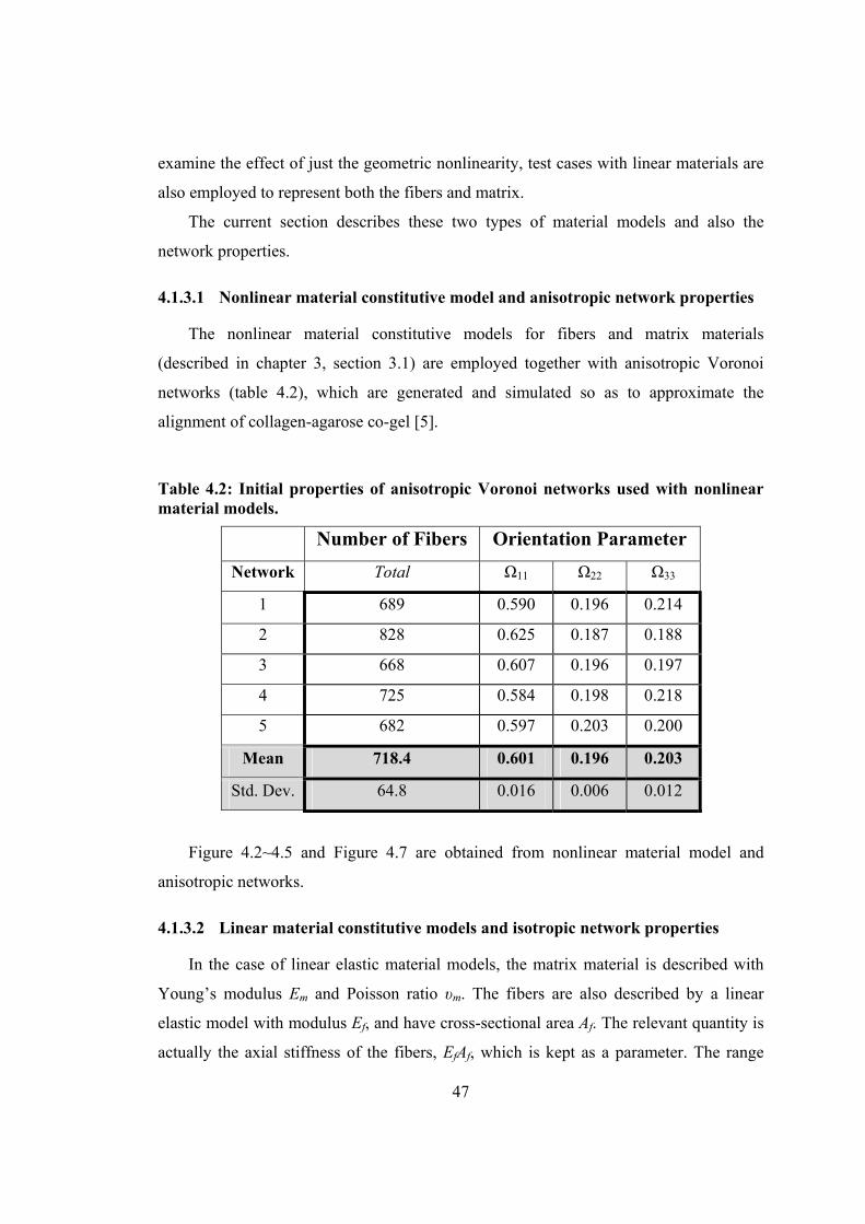
47

examine the effect of just the geometric nonlinearity, test cases with linear materials are

also employed to represent both the fibers and matrix.

The current section describes these two types of material models and also the

network properties.

4.1.3.1 Nonlinear material constitutive model and anisotropic network properties

The nonlinear material constitutive models for fibers and matrix materials

(described in chapter 3, section 3.1) are employed together with anisotropic Voronoi

networks (table 4.2), which are generated and simulated so as to approximate the

alignment of collagen-agarose co-gel [5].

Table 4.2: Initial properties of anisotropic Voronoi networks used with nonlinear material models.

Number of Fibers Orientation Parameter

Network Total Ω11 Ω22 Ω33

1 689 0.590 0.196 0.214

2 828 0.625 0.187 0.188

3 668 0.607 0.196 0.197

4 725 0.584 0.198 0.218

5 682 0.597 0.203 0.200

Mean 718.4 0.601 0.196 0.203

Std. Dev. 64.8 0.016 0.006 0.012

Figure 4.2~4.5 and Figure 4.7 are obtained from nonlinear material model and

anisotropic networks.

4.1.3.2 Linear material constitutive models and isotropic network properties

In the case of linear elastic material models, the matrix material is described with

Young’s modulus Em and Poisson ratio υm. The fibers are also described by a linear

elastic model with modulus Ef, and have cross-sectional area Af. The relevant quantity is

actually the axial stiffness of the fibers, EfAf, which is kept as a parameter. The range

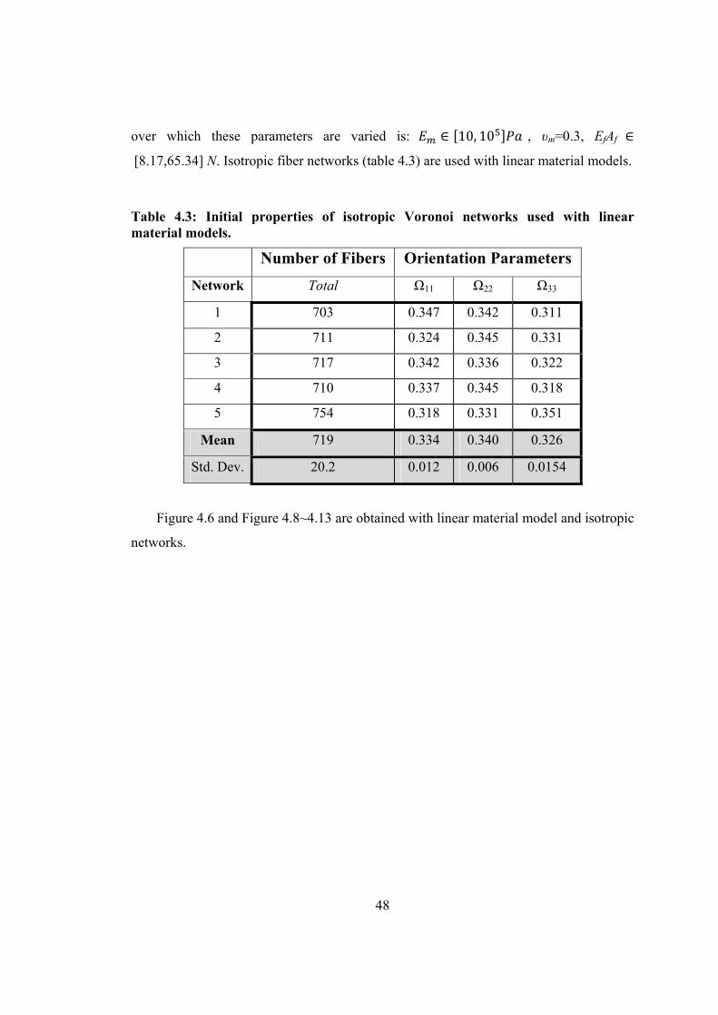
48

over which these parameters are varied is: ∈ 10, 10 , υm=0.3, EfAf ∈

[8.17,65.34] N. Isotropic fiber networks (table 4.3) are used with linear material models.

Table 4.3: Initial properties of isotropic Voronoi networks used with linear material models.

Number of Fibers Orientation Parameters

Network Total Ω11 Ω22 Ω33

1 703 0.347 0.342 0.311

2 711 0.324 0.345 0.331

3 717 0.342 0.336 0.322

4 710 0.337 0.345 0.318

5 754 0.318 0.331 0.351

Mean 719 0.334 0.340 0.326

Std. Dev. 20.2 0.012 0.006 0.0154

Figure 4.6 and Figure 4.8~4.13 are obtained with linear material model and isotropic

networks.

49

4.2 Overall RVE constitutive response

4.2.1 Overall RVE constitutive response with nonlinear materials

The RVE constitutive responses under tensile loading are described by reporting (1)

the averaged network stress 11ˆ n , (2) the averaged matrix stress 11ˆ m , (3) the averaged

total stress, 11 (4) the apparent Poisson’s ratio app (Eq. 4.1) .

The overall Cauchy stress, 11 , is evaluated based on the reactions evaluated on the

face with normal in the x1 direction, and the current area of the respective model

boundary segment. Formally one may refer to stresses associated with the network and

with the matrix, i.e. 11 11 11ˆ ˆ ˆm n , the two components being computed with the

reactions acting at the nodes where the network intersects the model boundary and those

corresponding to matrix elements, respectively.

The apparent Poisson’s ratio app is obtained by averaging 12 and 13 (Eq. 4.1),

which are apparent Poisson’s ratio in directions x1 and x2 and directions x1 and x3

respectively.

3212 13

1 1

lnlnˆ ˆ,

ln ln

(4.1a)

12 13

appˆ2

(4.1b)

where λ1, λ2 and λ3 are stretch ratios of the RVE along x1, x2 and x3 axes respectively.

Since nodal displacements on traction-free surfaces normal to x2 and x3 direction are not

constrained, λ2 and λ3 are calculated by averaging the associated displacement

component over all boundary nodes on surfaces normal to x2 and x3 axes respectively.

In the coupled fiber-matrix model 1 , the stress due to the fiber network 11ˆ n

increases with increasing non-fibrillar matrix (NFM) shear modulus Gm, and the non-

linearity of fiber stress-strain curves become less pronounced at higher Gm values

1 Portions of this chapter previously appeared as: (1) L. Zhang, S. P. Lake, V. K. Lai, C. R. Picu, V. H. Barocas, and M. S. Shephard, “A coupled fiber-matrix model demonstrates highly inhomogeneous microstructural interactions in soft tissues under tensile load,” J. Biomech. Eng., vol. 135, p. 011008, Jan. 2013, and (2) L. Zhang, S. P. Lake, V. H. Barocas, M. S. Shephard, and R. C. Picu, “Cross-linked fiber network embedded in an elastic matrix,” Soft Matter, vol. 9, p. 6398, 2013.

50

a)

(Figure 4.2(a)). As one might expect, the matrix stress 11ˆ m increases with increasing

NFM shear modulus (Figure 4.2(b)), which accounts for much of the increase in total

stress (Figure 4.2(c)). The RVE Poisson’s ratio decreases with increasing Gm, but

increases with strain for Gm =10 and 110 Pa (Figure 4.2(d)).

In addition to comparing model results computed at the same imposed strain, results

are also evaluated at the same imposed total stress 11 (in this case, 200 Pa). Matrix

stress values 11ˆ m increase with increasing shear modulus for both cases (Figure 4.3(a)).

In contrast, fiber stress 11ˆ n values increase for the constant strain case, but decrease for

the constant total stress case (Figure 4.3(b)), with the stiffer NFM shielding the network.

11ˆ [

Pa]

n

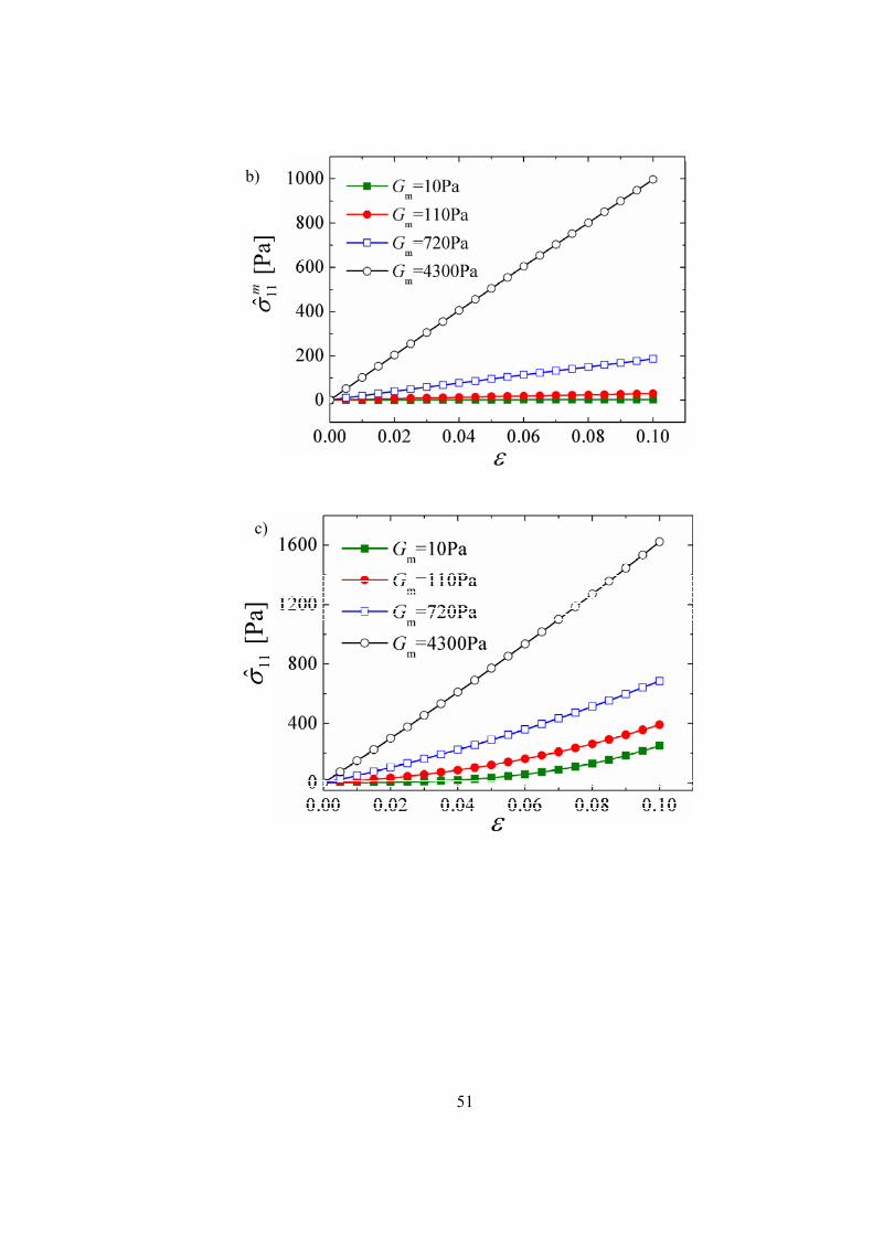
51

b)

c)

11ˆ [

Pa]

m

11ˆ [

Pa]

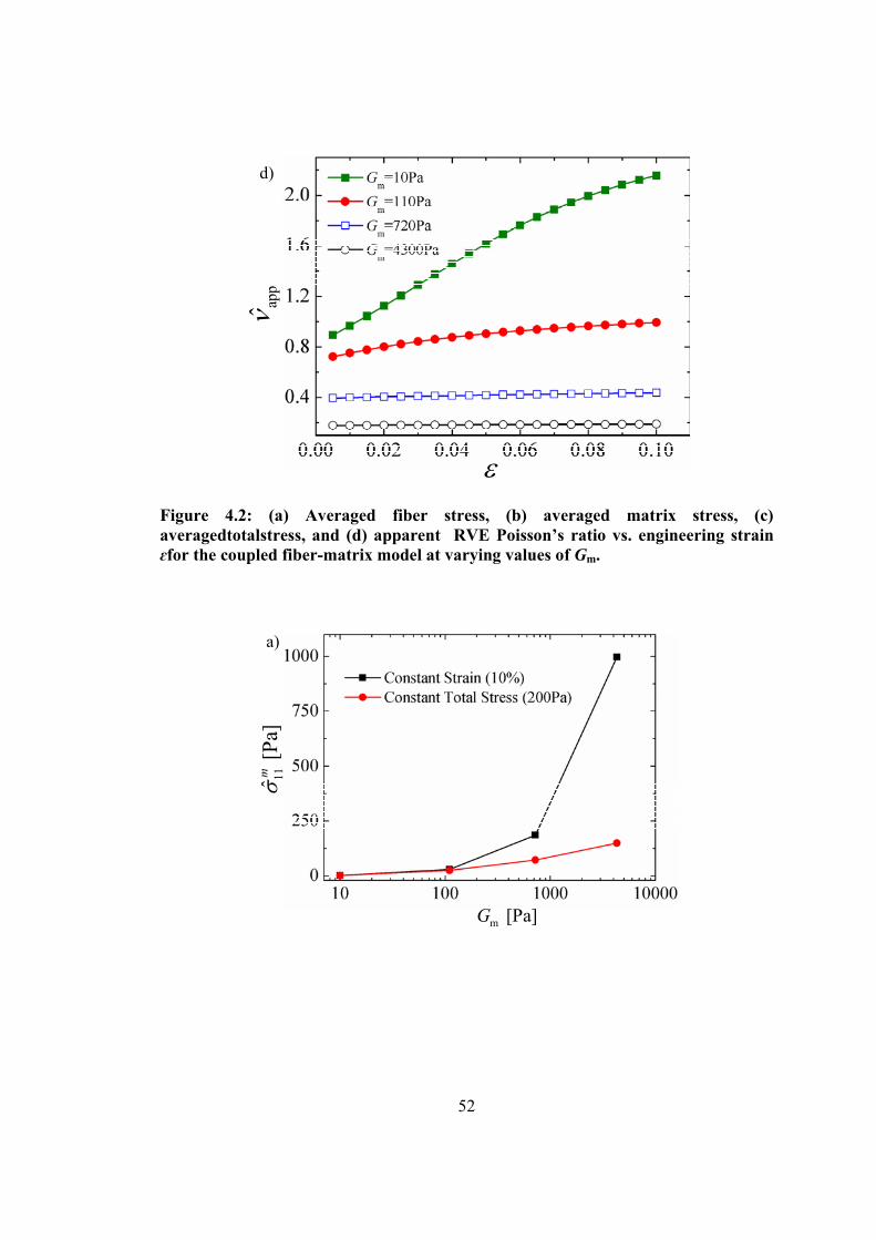
52

d)

a)

app

Figure 4.2: (a) Averaged fiber stress, (b) averaged matrix stress, (c) averagedtotalstress, and (d) apparent RVE Poisson’s ratio vs. engineering strain ɛfor the coupled fiber-matrix model at varying values of Gm.

11ˆ [

Pa]

m

m [Pa]G

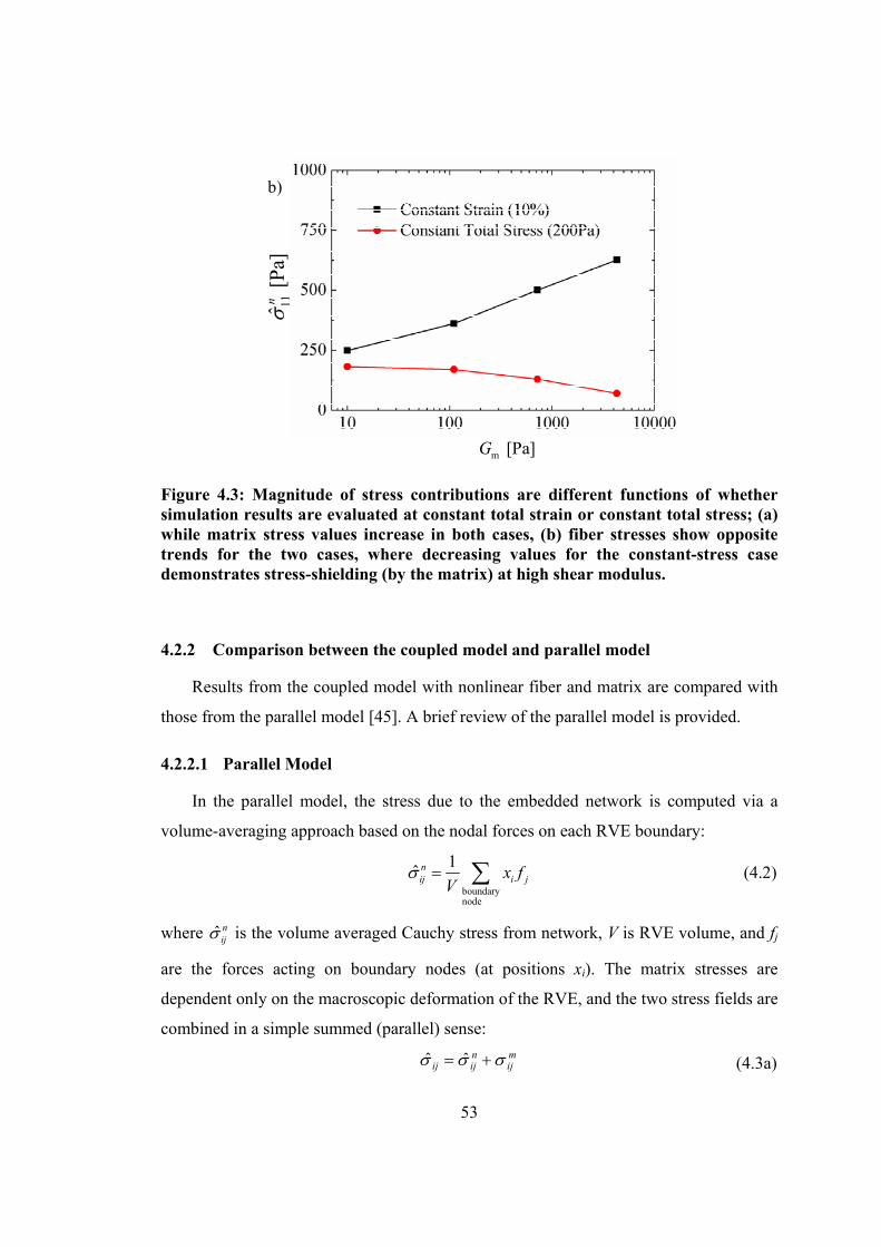
53

b)

m [Pa]G

11ˆ [

Pa]

n

Figure 4.3: Magnitude of stress contributions are different functions of whether simulation results are evaluated at constant total strain or constant total stress; (a) while matrix stress values increase in both cases, (b) fiber stresses show opposite trends for the two cases, where decreasing values for the constant-stress case demonstrates stress-shielding (by the matrix) at high shear modulus.

4.2.2 Comparison between the coupled model and parallel model

Results from the coupled model with nonlinear fiber and matrix are compared with

those from the parallel model [45]. A brief review of the parallel model is provided.

4.2.2.1 Parallel Model

In the parallel model, the stress due to the embedded network is computed via a

volume-averaging approach based on the nodal forces on each RVE boundary:

boundarynode

1ˆ n

ij i jx fV

(4.2)

where ˆ nij is the volume averaged Cauchy stress from network, V is RVE volume, and fj

are the forces acting on boundary nodes (at positions xi). The matrix stresses are

dependent only on the macroscopic deformation of the RVE, and the two stress fields are

combined in a simple summed (parallel) sense:

ˆ ˆ n m

ij ij ij (4.3a)

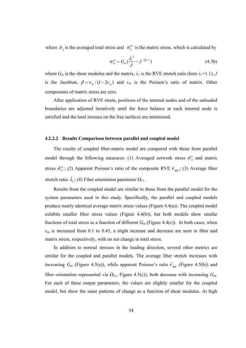
54

where ˆ ij is the averaged total stress and mij is the matrix stress, which is calculated by

22 11

11 ( )mmG J

J

(4.3b)

where Gm is the shear modulus and the matrix, λ1 is the RVE stretch ratio (here λ1=1.1), J

is the Jacobian, / (1 2 )m m and νm is the Poisson’s ratio of matrix. Other

components of matrix stress are zero.

After application of RVE strain, positions of the internal nodes and of the unloaded

boundaries are adjusted iteratively until the force balance at each internal node is

satisfied and the total stresses on the free surfaces are minimized.

4.2.2.2 Results Comparison between parallel and coupled model

The results of coupled fiber-matrix model are compared with those from parallel

model through the following measures: (1) Averaged network stress 11ˆ n and matrix

stress 11ˆ m ; (2) Apparent Poisson’s ratio of the composite RVE app ; (3) Average fiber

stretch ratio f ; (4) Fiber orientation parameter Ω11.

Results from the coupled model are similar to those from the parallel model for the

system parameters used in this study. Specifically, the parallel and coupled models

produce nearly identical average matrix stress values (Figure 4.4(a)). The coupled model

exhibits smaller fiber stress values (Figure 4.4(b)), but both models show similar

fractions of total stress as a function of different Gm (Figure 4.4(c)). In both cases, when

νm is increased from 0.1 to 0.45, a slight increase and decrease are seen in fiber and

matrix stress, respectively, with no net change in total stress.

In addition to normal stresses in the loading direction, several other metrics are

similar for the coupled and parallel models. The average fiber stretch increases with

increasing Gm (Figure 4.5(a)), while apparent Poisson’s ratio app (Figure 4.5(b)) and

fiber orientation represented via Ω11, Figure 4.5(c)), both decrease with increasing Gm.

For each of these output parameters, the values are slightly smaller for the coupled

model, but show the same patterns of change as a function of shear modulus. At high

55

a)

b)

NFM Poisson’s ratio (i.e., νm=0.45), f and app are slightly increased and decreased,

respectively, with no change in Ω11.

11ˆ [

Pa]

m

11ˆ [

Pa]

n

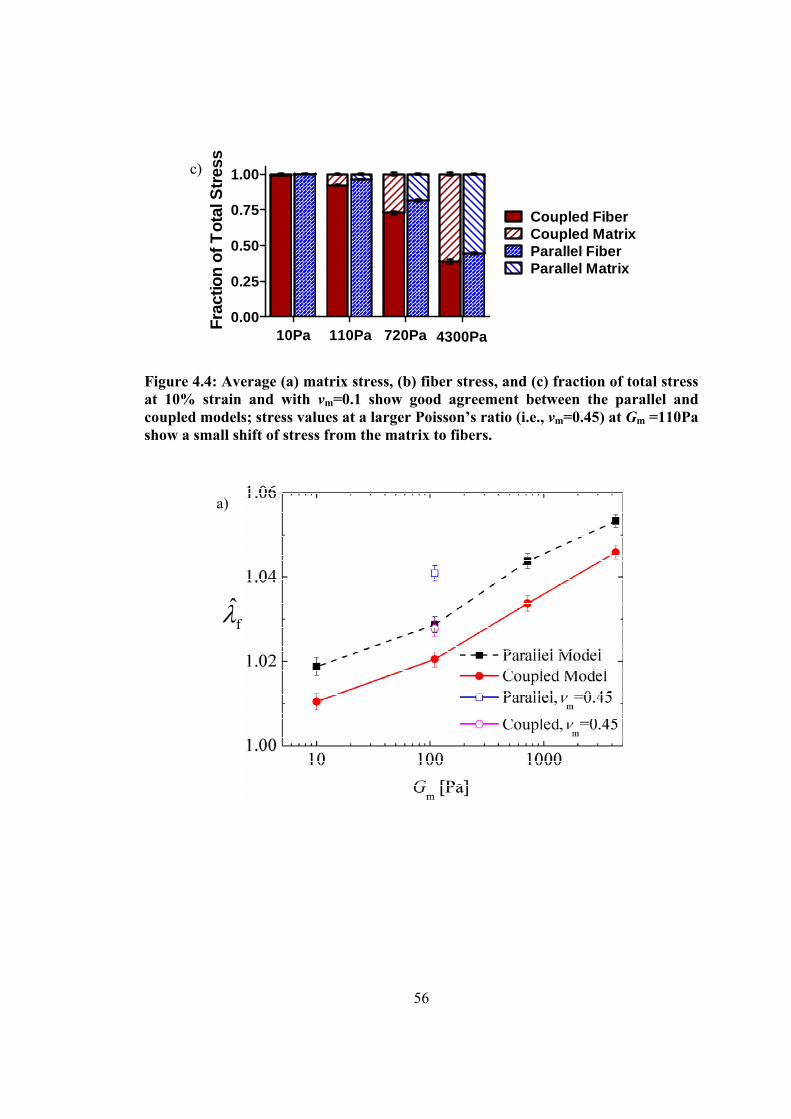
56

c)

a)

Figure 4.4: Average (a) matrix stress, (b) fiber stress, and (c) fraction of total stress at 10% strain and with νm=0.1 show good agreement between the parallel and coupled models; stress values at a larger Poisson’s ratio (i.e., νm=0.45) at Gm =110Pa show a small shift of stress from the matrix to fibers.

f

Fra

ctio

n o

f T

ota

l Str

ess

0.00

0.25

0.50

0.75

1.00

Coupled FiberCoupled Matrix

10Pa 110Pa 720Pa 4300Pa

Parallel FiberParallel Matrix

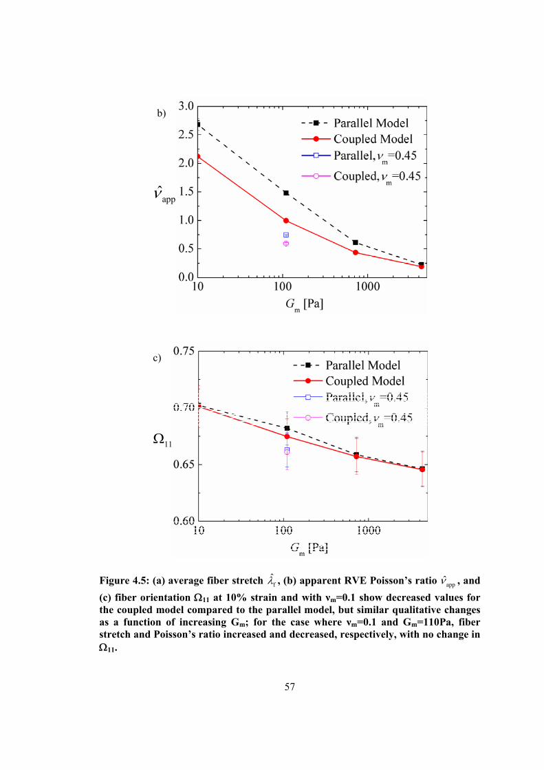
57

b)

c)

app

11

Figure 4.5: (a) average fiber stretch f , (b) apparent RVE Poisson’s ratio app , and

(c) fiber orientation 11 at 10% strain and with νm=0.1 show decreased values for the coupled model compared to the parallel model, but similar qualitative changes as a function of increasing Gm; for the case where νm=0.1 and Gm=110Pa, fiber stretch and Poisson’s ratio increased and decreased, respectively, with no change in 11.

58

4.2.3 RVE constitutive response with linear material models

To examine the effect of only the geometric nonlinearity on the RVE constitutive

response, a linear material model is employed to represent fiber and matrix in this

section [58]. The stress-strain curves of all systems considered are non-linear. The non-

linearity here is purely geometric since the constitutive equations of the matrix and fiber

materials are both linear. Figures 4.6(a) and 4.6(b) show the stress strain curves, ,

of two models with Em=10 and 104 Pa, respectively. The embedded network

characterized by EfAf = 8.168N and lc/L = 0.104, is embedded in the two matrices. The

filled symbols correspond to the total stress , while the open symbols correspond

to the component of the total stress associated with the network, . In the stiffer

matrix case (Figure 4.6(a)), the network contributes little to the overall modulus, as

expected, and the degree of non-linearity of is small. The situation is reversed in

the softer matrix case (Figure 4.6(b)). The non-linearity of the network is pronounced

and this reflects in . The data indicate the intuitive fact that the non-linearity in the

behavior of the network-matrix system is associated with the large geometric non-

linearity of the network. To make this effect more obvious, Figure 4.6(c) shows the

contribution to these stress-strain curves from the non-linear component. Denote by

the small strain effective modulus of the network-matrix system ( ⁄ for → 0),

and further, define / for → 0. The non-linear component is evaluated as

11 11ˆˆ ˆ( ) ( ( ) ) / ( )NL E (4.4)

The non-linearity is much more pronounced in the soft matrix case, while the network

component is always more non-linear than the total stress-strain curve.

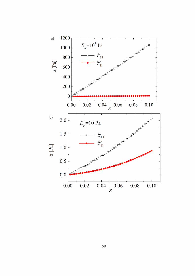
59

a)

b)

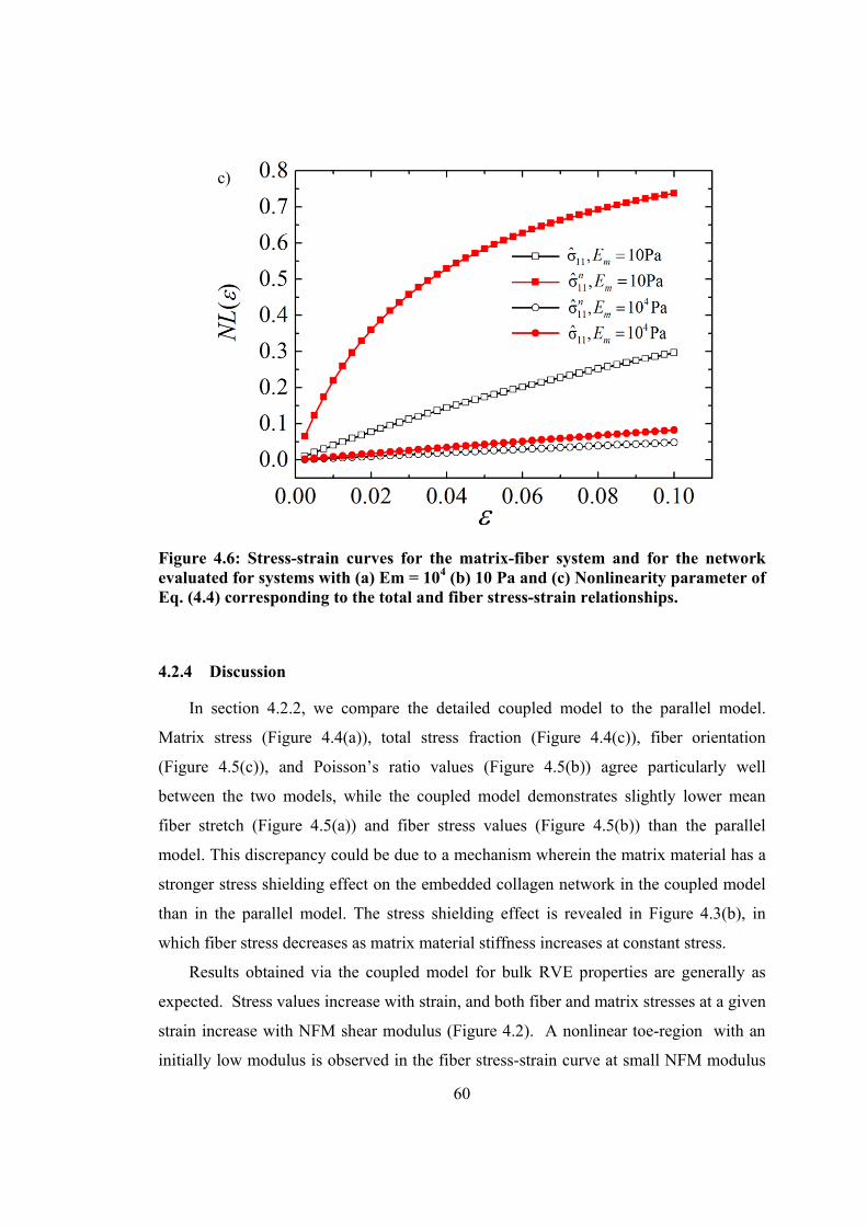
60

Figure 4.6: Stress-strain curves for the matrix-fiber system and for the network evaluated for systems with (a) Em = 104 (b) 10 Pa and (c) Nonlinearity parameter of Eq. (4.4) corresponding to the total and fiber stress-strain relationships.

4.2.4 Discussion

In section 4.2.2, we compare the detailed coupled model to the parallel model.

Matrix stress (Figure 4.4(a)), total stress fraction (Figure 4.4(c)), fiber orientation

(Figure 4.5(c)), and Poisson’s ratio values (Figure 4.5(b)) agree particularly well

between the two models, while the coupled model demonstrates slightly lower mean

fiber stretch (Figure 4.5(a)) and fiber stress values (Figure 4.5(b)) than the parallel

model. This discrepancy could be due to a mechanism wherein the matrix material has a

stronger stress shielding effect on the embedded collagen network in the coupled model

than in the parallel model. The stress shielding effect is revealed in Figure 4.3(b), in

which fiber stress decreases as matrix material stiffness increases at constant stress.

Results obtained via the coupled model for bulk RVE properties are generally as

expected. Stress values increase with strain, and both fiber and matrix stresses at a given

strain increase with NFM shear modulus (Figure 4.2). A nonlinear toe-region with an

initially low modulus is observed in the fiber stress-strain curve at small NFM modulus

c)

61

values, but nonlinearity is less pronounced at larger NFM modulus values. The tendency

toward linearity is consistent with a stiffer matrix eliminating the non-affine, low-stretch

reorientation of the fiber network, which is proved in subsequent sections on the

interactions between the two constituents.

In addition, the nonlinear relationship of Poisson’s ratio and strain at low Gm

(Figure 4.2(d)) closely matched the relationship observed in experimental tests of

collagen-agarose co-gels [5]. The bulk RVE stresses analyzed in this model are obtained

from simulations at a constant strain value (e.g., 10% stretch). When results are

computed at a constant total stress (200 Pa) for each of the varied simulations, fiber

stresses decrease with increasing NFM modulus, demonstrating a stress shielding role of

the NFM at large Gm.

4.3 Effect of fiber network on matrix – the case of linear material models

This section focuses on investigating the effect of the fiber network on the matrix

material. The effect is outlined by analyzing (1) the probability distribution function of

matrix element stresses, and (2) the variation of stress within the matrix. Obviously, the

matrix without the embedded network deforms affinely and, in this case, the stress is

uniform throughout.

4.3.1 Inhomogeneous stress distribution in the matrix

The use of the coupled model allows for full-field quantification of the six

independent Cauchy stress components of the matrix material, visualized via slice plots

through the RVE midsection. The embedded fiber network had a significant effect on

the stress field of the surrounding matrix material, as demonstrated by the

inhomogeneity of the internal stress distribution. Figure 4.7 shows representative plots of

stress fields for the system with matrix shear modulus Gm = 720 Pa. The black dots in

Figure 4.7 represent the intersection points between fibers and the cutting plane.

Tensile normal stresses (i.e., positive values) are evident in the loading direction

(σ11), whereas compressive stresses are observed in the transverse directions (e.g., σ22

and σ33) in response to the extreme tendency of the collagen network to contract in the

62

transverse directions. Stress concentrations (either positive or negative) occur at

locations where two or more fibers traverse the slice plane in close proximity.

The tensile normal stresses in the loading direction (σ11) are relatively consistent

across the RVEs, although smaller values are observed in the vicinity of multiple fiber

intersection points. Compressive normal stresses in traverse directions (i.e., σ22 and σ33)

are caused by fibers squeezing the surrounding matrix material in the lateral direction

during reorientation. Due to the Poisson effect, the matrix material is compressed in the

lateral directions as it is concurrently stretched in the loading direction, thereby

decreasing the local tensile stress and leading to smaller σ11 values in areas of

concentrated fiber intersection points. Maps of internal shear stresses demonstrate

complex patterns (Figure 4.7(bottom)), with areas of particularly high shear stress co-

localized with significant fiber clustering.

Figure 4.7: Interior normal and shear stress fields at 10% strain on the mid-section slice for a representative network (Gm=720Pa; νm=0.1) demonstrates a highly inhomogeneous distribution for all six independent stress components; slices are cut normal to the loading (x1) direction in the 2-3 plane (represented by the dashed lines in the RVE schematic) and black dots indicate locations of fibers intersecting the cutting plane.

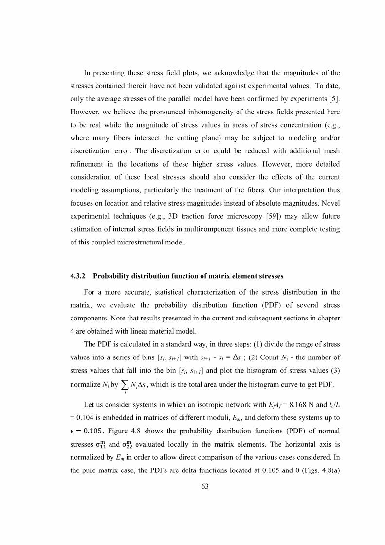
63

In presenting these stress field plots, we acknowledge that the magnitudes of the

stresses contained therein have not been validated against experimental values. To date,

only the average stresses of the parallel model have been confirmed by experiments [5].

However, we believe the pronounced inhomogeneity of the stress fields presented here

to be real while the magnitude of stress values in areas of stress concentration (e.g.,

where many fibers intersect the cutting plane) may be subject to modeling and/or

discretization error. The discretization error could be reduced with additional mesh

refinement in the locations of these higher stress values. However, more detailed

consideration of these local stresses should also consider the effects of the current

modeling assumptions, particularly the treatment of the fibers. Our interpretation thus

focuses on location and relative stress magnitudes instead of absolute magnitudes. Novel

experimental techniques (e.g., 3D traction force microscopy [59]) may allow future

estimation of internal stress fields in multicomponent tissues and more complete testing

of this coupled microstructural model.

4.3.2 Probability distribution function of matrix element stresses

For a more accurate, statistical characterization of the stress distribution in the

matrix, we evaluate the probability distribution function (PDF) of several stress

components. Note that results presented in the current and subsequent sections in chapter

4 are obtained with linear material model.

The PDF is calculated in a standard way, in three steps: (1) divide the range of stress

values into a series of bins [si, si+1] with si+1 - si = ∆s ; (2) Count Ni - the number of

stress values that fall into the bin [si, si+1] and plot the histogram of stress values (3)

normalize Ni by ii

N s , which is the total area under the histogram curve to get PDF.

Let us consider systems in which an isotropic network with EfAf = 8.168 N and lc/L

= 0.104 is embedded in matrices of different moduli, Em, and deform these systems up to

ϵ 0.105. Figure 4.8 shows the probability distribution functions (PDF) of normal

stresses σ and σ evaluated locally in the matrix elements. The horizontal axis is

normalized by Em in order to allow direct comparison of the various cases considered. In

the pure matrix case, the PDFs are delta functions located at 0.105 and 0 (Figs. 4.8(a)

64

and 4.8(b), respectively) corresponding to σ and σ . In presence of the network, the

PDFs are broad, with the second moment increasing as Em decreases. Hence, the network

induces large spatial stress variability in soft matrices. This is an important observation

since the stress states control fracture and damage accumulation during fatigue loading.

Figure 4.8: Probability distribution functions of normalized (a) and (b) computed in the matrix. The stress is normalized with the matrix modulus, Em.

b)

a)

65

It is also interesting to observe that the means of the PDFs in Figure 4.8(a) shift to

smaller values as the matrix stiffness decreases. In other words, when subjected to the

same global strain, a system with a softer matrix would carry smaller normalized stresses

(normalization with Em) than a system with a stiffer matrix. A similar effect is observed

in Figure 4.8(b)) where it is seen that the mean increases in absolute value as Em

decreases. This effect was discussed in [52] and it is due to the fact that the network

subjected to tension has a Poisson ratio much larger than that of the matrix. Therefore,

when the same strain is imposed in the x1 direction on the network and matrix, the

network tends to shrink more in the x2 and x3 directions, therefore compressing the

matrix. This leads to a mean compressive stress in x2 and x3, and, due to the Poisson

effect of the matrix, to unloading in the x1 direction.

4.3.3 Locations of stress concentration in the matrix material

Since the fibers are represented by straight truss segments in this model, the

interaction between network and matrix takes place exclusively through forces applied

by the network on the matrix at the cross-links. The situation is expected to remain

qualitatively similar even in presence of moderate fiber crimp and curl and when the

interface between fibers and matrix are weak. This leads to significant stress

concentration and a highly heterogeneous stress field characterized by the broad

distributions of Figure 4.8. To demonstrate the presence of such concentration sites, the

locations (Gauss points) where stress is larger than a specified threshold are identified

and the pair correlation function, g(r), of these points is computed. A brief explanation of

the calculation of g(r) is as follows:

Calculation of the pair correlation function g(r)

(1) Create a series of concentric spherical bins with radius rj (j=1,2,…, maxiN )

centered at each fiber crosslink i within the RVE (see Figure 4.9). maxiN is the

number of concentric bins centered at crosslink i inside the RVE. The volume of

each bin Vj is

3 31

4( ),

3j j j jV r r r j r (4.5)

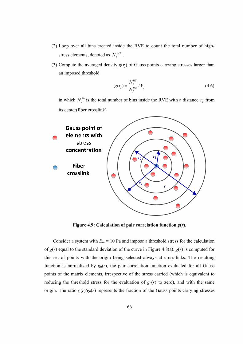
66

(2) Loop over all bins created inside the RVE to count the total number of high-

stress elements, denoted as HSjN .

(3) Compute the averaged density g(rj) of Gauss points carrying stresses larger than

an imposed threshold.

(r ) /

HSj

j jBinj

Ng V

N

(4.6)

in which BinjN is the total number of bins inside the RVE with a distance jr from

its center(fiber crosslink).

Figure 4.9: Calculation of pair correlation function g(r).

Consider a system with Em = 10 Pa and impose a threshold stress for the calculation

of g(r) equal to the standard deviation of the curve in Figure 4.8(a). g(r) is computed for

this set of points with the origin being selected always at cross-links. The resulting

function is normalized by g0(r), the pair correlation function evaluated for all Gauss

points of the matrix elements, irrespective of the stress carried (which is equivalent to

reducing the threshold stress for the evaluation of g0(r) to zero), and with the same

origin. The ratio g(r)/g0(r) represents the fraction of the Gauss points carrying stresses

67

larger than the imposed threshold (Figure 4.10). It is clear that large stresses are found

predominantly close to the cross-links of the network (r → 0). The asymptote at larger

values of the variable represents the fraction of all Gauss points of the model carrying

stresses larger than the imposed threshold.

Figure 4.10: Normalized pair correlation function g(r) indicating stress concentration close to the network cross-links (i.e. at → ).

4.4 Effect of matrix material on the fiber network – the case of linear material models

Networks of trusses are known to be unstable if the coordination number, z, is

smaller than 2d, where d is the dimensionality of the embedding space [60]. Networks

with lower coordination numbers are floppy and deform without storing energy. The

networks considered in this study have coordination number z = 4, smaller than the value

of 6 required for stability and hence are intrinsically floppy. As discussed in the

literature [23, 28, 60], a floppy network can be stabilized by accounting for the bending

stiffness of fibers and by transforming the cross-links into connectors that transmit both

moments and forces between the fibers in contact. A floppy network acquires stiffness

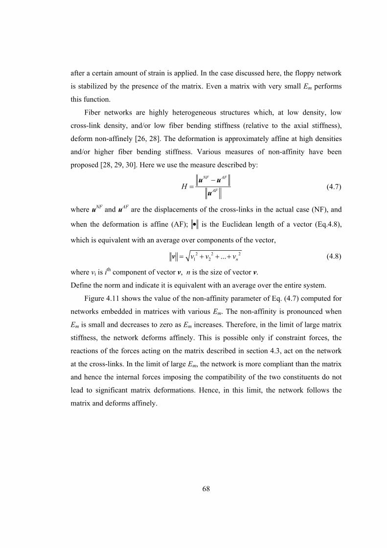
68

after a certain amount of strain is applied. In the case discussed here, the floppy network

is stabilized by the presence of the matrix. Even a matrix with very small Em performs

this function.

Fiber networks are highly heterogeneous structures which, at low density, low

cross-link density, and/or low fiber bending stiffness (relative to the axial stiffness),

deform non-affinely [26, 28]. The deformation is approximately affine at high densities

and/or higher fiber bending stiffness. Various measures of non-affinity have been

proposed [28, 29, 30]. Here we use the measure described by:

NF AF

AFH

u u

u

(4.7)

where uNF and uAF are the displacements of the cross-links in the actual case (NF), and

when the deformation is affine (AF); is the Euclidean length of a vector (Eq.4.8),

which is equivalent with an average over components of the vector,

2 2 2

1 2 ... nv v v v

(4.8)

where vi is ith component of vector v, n is the size of vector v.

Define the norm and indicate it is equivalent with an average over the entire system.

Figure 4.11 shows the value of the non-affinity parameter of Eq. (4.7) computed for

networks embedded in matrices with various Em. The non-affinity is pronounced when

Em is small and decreases to zero as Em increases. Therefore, in the limit of large matrix

stiffness, the network deforms affinely. This is possible only if constraint forces, the

reactions of the forces acting on the matrix described in section 4.3, act on the network

at the cross-links. In the limit of large Em, the network is more compliant than the matrix

and hence the internal forces imposing the compatibility of the two constituents do not

lead to significant matrix deformations. Hence, in this limit, the network follows the

matrix and deforms affinely.

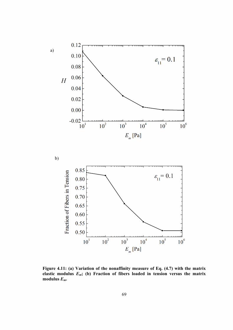
69

Figure 4.11: (a) Variation of the nonaffinity measure of Eq. (4.7) with the matrix elastic modulus Em; (b) Fraction of fibers loaded in tension versus the matrix modulus Em.

a)

b)

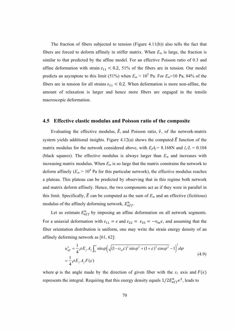
70

The fraction of fibers subjected to tension (Figure 4.11(b)) also tells the fact that

fibers are forced to deform affinely in stiffer matrix. When Em is large, the fraction is

similar to that predicted by the affine model. For an effective Poisson ratio of 0.3 and

affine deformation with strain 0.2, 51% of the fibers are in tension. Our model

predicts an asymptote to this limit (51%) when Em > 105 Pa. For Em=10 Pa, 84% of the

fibers are in tension for all strains 0.2. When deformation is more non-affine, the

amount of relaxation is larger and hence more fibers are engaged in the tensile

macroscopic deformation.

4.5 Effective elastic modulus and Poisson ratio of the composite

Evaluating the effective modulus, , and Poisson ratio, , of the network-matrix

system yields additional insights. Figure 4.12(a) shows the computed function of the

matrix modulus for the network considered above, with EfAf = 8.168N and lc/L = 0.104

(black squares). The effective modulus is always larger than Em and increases with

increasing matrix modulus. When Em is so large that the matrix constrains the network to

deform affinely (Em > 104 Pa for this particular network), the effective modulus reaches

a plateau. This plateau can be predicted by observing that in this regime both network

and matrix deform affinely. Hence, the two components act as if they were in parallel in

this limit. Specifically, can be computed as the sum of Em and an effective (fictitious)

modulus of the affinely deforming network, .

Let us estimate by imposing an affine deformation on all network segments.

For a uniaxial deformation with and , and assuming that the

fiber orientation distribution is uniform, one may write the strain energy density of an

affinely deforming network as [61, 62]:

22 2 2 2

0

1sin (1 ) sin (1 ) cos 1

41

( )4

naff f f m

f f

u E A d

E A F

(4.9)

where is the angle made by the direction of given fiber with the x1 axis and

represents the integral. Requiring that this energy density equals 1/2 , leads to

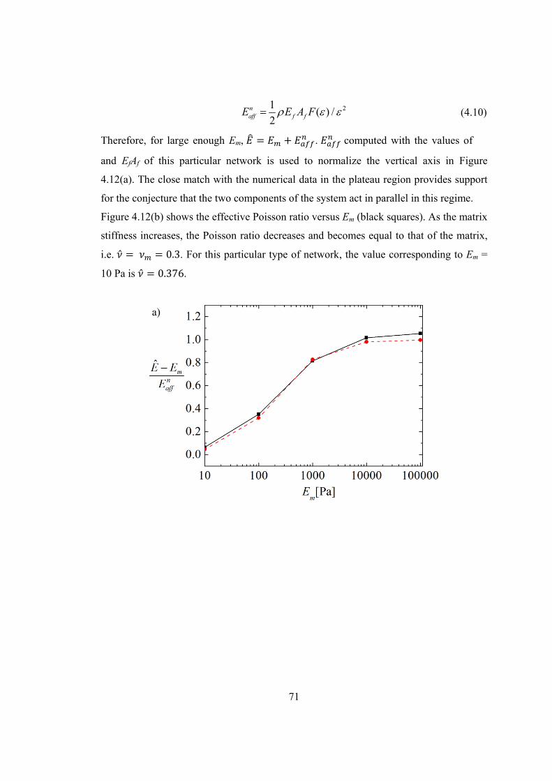
71

21( ) /

2naff f fE E A F

(4.10)

Therefore, for large enough Em, . computed with the values of 　

and EfAf of this particular network is used to normalize the vertical axis in Figure

4.12(a). The close match with the numerical data in the plateau region provides support

for the conjecture that the two components of the system act in parallel in this regime.

Figure 4.12(b) shows the effective Poisson ratio versus Em (black squares). As the matrix

stiffness increases, the Poisson ratio decreases and becomes equal to that of the matrix,

i.e. 0.3. For this particular type of network, the value corresponding to Em =

10 Pa is 0.376.

a)

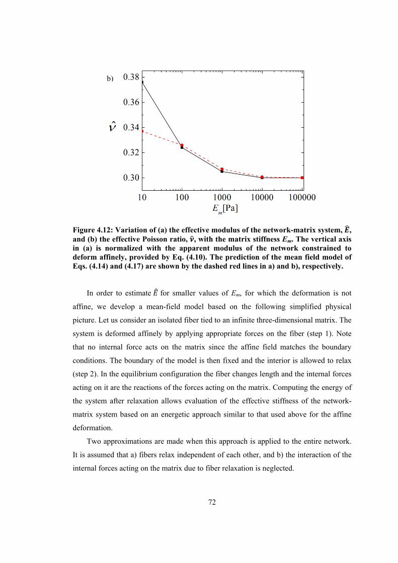
72

Figure 4.12: Variation of (a) the effective modulus of the network-matrix system, , and (b) the effective Poisson ratio, , with the matrix stiffness Em. The vertical axis in (a) is normalized with the apparent modulus of the network constrained to deform affinely, provided by Eq. (4.10). The prediction of the mean field model of Eqs. (4.14) and (4.17) are shown by the dashed red lines in a) and b), respectively.

In order to estimate for smaller values of Em, for which the deformation is not

affine, we develop a mean-field model based on the following simplified physical

picture. Let us consider an isolated fiber tied to an infinite three-dimensional matrix. The

system is deformed affinely by applying appropriate forces on the fiber (step 1). Note

that no internal force acts on the matrix since the affine field matches the boundary

conditions. The boundary of the model is then fixed and the interior is allowed to relax

(step 2). In the equilibrium configuration the fiber changes length and the internal forces

acting on it are the reactions of the forces acting on the matrix. Computing the energy of

the system after relaxation allows evaluation of the effective stiffness of the network-

matrix system based on an energetic approach similar to that used above for the affine

deformation.

Two approximations are made when this approach is applied to the entire network.

It is assumed that a) fibers relax independent of each other, and b) the interaction of the

internal forces acting on the matrix due to fiber relaxation is neglected.

b)

73

The strain energy density of the network during the relaxation of step 2 is computed

by assuming that each fiber relaxes by a fraction β of its affine deformation of step 1.

Then,

21( ) (1 ) ( )

4n

f fu E A F

(4.11)

The total energy stored in the matrix during the relaxation process is equal to the work

performed by the internal forces. For each fiber, there are a pair of forces aligned with

the fiber and acting on the matrix in opposite directions at the location of the two ends of

the fiber. Under the assumption that these internal forces do not interact, the problem is

equivalent to computing the work done by a force P acting on an infinite isotropic

continuum, i.e. /2, where δ is the displacement of the point where P acts. Note that P

is equal to the force stretching the bar and leading to the strain energy density of Eq.

(4.11). Using the Green’s function solution for an isotropic three-dimensional solid [64],

one can write:

22 2 2 2 2 21 1

(1 ) sin (1 ) cos 12 2

mf m

EP L d

(4.12)

In the Green’s function solution, the energy stored in the body diverges and the solution

predicts → ∞. To avoid this problem, an inner spherical cut-off of radius Rmin needs to

be taken in the vicinity of the force P. Parameter α in Eq. (4.12) depends on and Rmin

as / , and hence has units of inverse length. Function h reads

12 10 11 11 / 24 1 . With this, the strain energy density stored

in the matrix due to the relaxation of all (non-interacting) fibers is evaluated as:

21( ) ( )

4m m

c

Eu l F

(4.13)

Here we have taken , the mean fiber length. Finding the minimum (with respect

to β) of the total strain energy density leads to 1/ 1 ,

where is a non-dimensional parameter.

With this, one may compute the total strain energy stored and the effective modulus

of the network-matrix system, which can be written as:

ˆ1

nm affE E E

(4.14)

74

Figure 4.13 shows the effective modulus of the network-matrix system,

/ , versus / 1 for several networks with different lc/L (in the range 0.1 to

0.2) and EfAf (in the range 8.17 to 65.34 N) and embedded in matrices with Em ranging

from 10 to 104 Pa. The same value for parameter α (i.e. α = 4/3) is used for all curves.

The data collapse on the line of slope 1, providing support to Eq. (4.14). The prediction

of Eq. (4.14) is also added to Figure 4.12(a) and is seen to provide a good representation

of the data.

The effective Poisson ratio of the material can be determined using the same model.

Each fiber oriented at an angle with respect to the loading direction acts on the matrix

with a force given by (after the relaxation of step 2):

2 2 2 2(1 ) (1 ) sin (1 ) cos 1f f mP E A

(4.15)

which has a component in the direction perpendicular to the loading direction of

magnitude . The planar density of fibers with orientation between and

crossing a plane parallel to the loading direction is 1 2⁄ , and the

effective normal stress produced by these fibers perpendicular to the loading direction

can be computed as sin . The average normal strain in the matrix in the x2

direction due to the action of the network results by summing contributions of fibers

with all orientations:

/2 2 2 2 2 322 0

1(1 ) (1 ) sin (1 ) cos 1 sin

2

1(1 ) ( )

2

f f mm

f fm

E A dE

E A GE

(4.16)

where represents the integral. After adding the Poisson effect of the matrix, the

effective Poisson ratio can be written:

0 22 0

( )1ˆ lim / lim

2 1f

m m fm

E GA

E

(4.17)

The prediction of Eq. (4.17) is shown in Figure 4.11(b) with dashed line and is seen

to be in good agreement with the values computed with the numerical model. The

agreement is not as good at the lowest value of the matrix modulus.

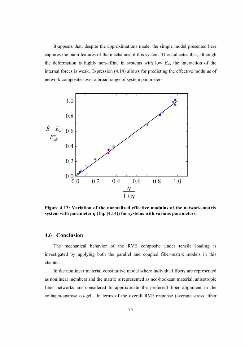
75

It appears that, despite the approximations made, the simple model presented here

captures the main features of the mechanics of this system. This indicates that, although

the deformation is highly non-affine in systems with low Em, the interaction of the

internal forces is weak. Expression (4.14) allows for predicting the effective modulus of

network composites over a broad range of system parameters.

Figure 4.13: Variation of the normalized effective modulus of the network-matrix system with parameter η (Eq. (4.14)) for systems with various parameters.

4.6 Conclusion

The mechanical behavior of the RVE composite under tensile loading is

investigated by applying both the parallel and coupled fiber-matrix models in this

chapter.

In the nonlinear material constitutive model where individual fibers are represented

as nonlinear members and the matrix is represented as neo-hookean material, anisotropic

fiber networks are considered to approximate the preferred fiber alignment in the

collagen-agarose co-gel. In terms of the overall RVE response (average stress, fiber

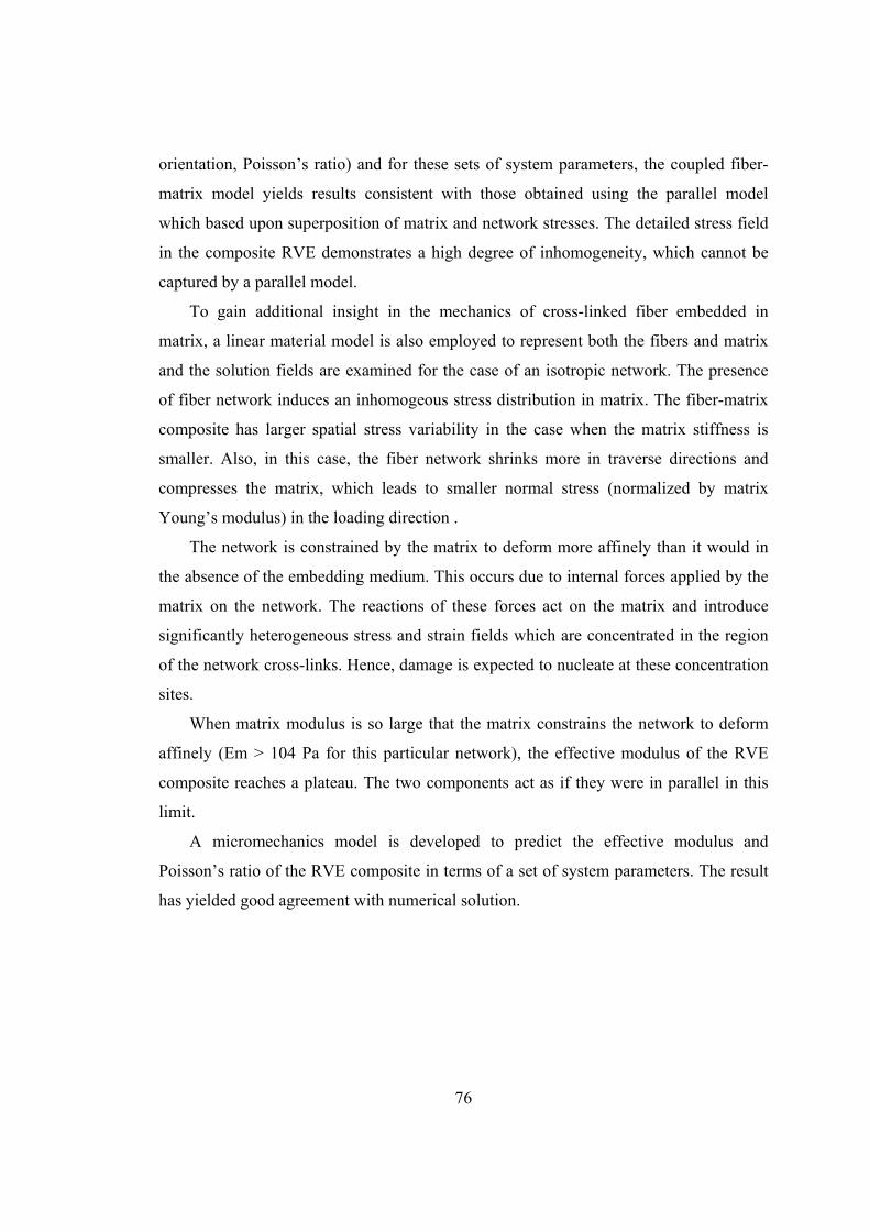
76

orientation, Poisson’s ratio) and for these sets of system parameters, the coupled fiber-

matrix model yields results consistent with those obtained using the parallel model

which based upon superposition of matrix and network stresses. The detailed stress field

in the composite RVE demonstrates a high degree of inhomogeneity, which cannot be

captured by a parallel model.


matrix, a linear material model is also employed to represent both the fibers and matrix

and the solution fields are examined for the case of an isotropic network. The presence

of fiber network induces an inhomogeous stress distribution in matrix. The fiber-matrix

composite has larger spatial stress variability in the case when the matrix stiffness is

smaller. Also, in this case, the fiber network shrinks more in traverse directions and

compresses the matrix, which leads to smaller normal stress (normalized by matrix

Young’s modulus) in the loading direction .

The network is constrained by the matrix to deform more affinely than it would in

the absence of the embedding medium. This occurs due to internal forces applied by the

matrix on the network. The reactions of these forces act on the matrix and introduce

significantly heterogeneous stress and strain fields which are concentrated in the region

of the network cross-links. Hence, damage is expected to nucleate at these concentration

sites.

When matrix modulus is so large that the matrix constrains the network to deform

affinely (Em > 104 Pa for this particular network), the effective modulus of the RVE

composite reaches a plateau. The two components act as if they were in parallel in this

limit.

A micromechanics model is developed to predict the effective modulus and

Poisson’s ratio of the RVE composite in terms of a set of system parameters. The result

has yielded good agreement with numerical solution.

77

5. Volume averaging-based multiscale model

5.1 Introduction

The macroscopic behaviors of soft tissue are largely governed by the underlying

microstructure. The volume averaging-based multiscale theory [48, 64] provides an

effective way to directly link the mechanics of microstructure to the overall tissue

mechanics. Hence, the proper mechanical modeling of microstructure is essential to the

prediction of multiscale approach. As discussed in previous chapters, matrix plays an

important role in affecting the network behaviors. Although the ultimate goal of the

multiscale approach is to incorporate the contribution from both matrix and fiber

network, for example, by employing the coupled fiber-matrix model at the representative

volume element level, this chapter presents a general multiscale scheme to effectively

incorporate the response of fiber network into the overall tissue mechanics.

In the present study, the microscale is represented as a three-dimensional

interconnected fiber networks which transmit uniaxial forces through crosslinks. The

crosslinked fiber network is contained in a representative volume element, which is

constructed separately at each Gauss point of finite elements representing the

macroscopic domain (Figure 5.1). In the multiscale scheme, the material constitutive

model is not required at the macroscopic scale; instead, the local stress-strain response is

obtained by solving a RVE boundary value problem at each Gauss point. After the RVE

problem is solved, the averaged Cauchy stress is returned to the macroscopic scale to

formulate nonlinear finite element equations.

Macroscopic scale One finite element at macro-scale

Microscopic scale(RVE)

Figure 5.1: Illustration of the multiscale approach for soft tissue analysis.

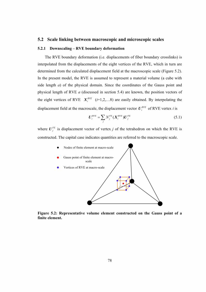
78

5.2 Scale linking between macroscopic and microscopic scales

5.2.1 Downscaling – RVE boundary deformation

The RVE boundary deformation (i.e. displacements of fiber boundary crosslinks) is

interpolated from the displacements of the eight vertices of the RVE, which in turn are

determined from the calculated displacement field at the macroscopic scale (Figure 5.2).

In the present model, the RVE is assumed to represent a material volume (a cube with

side length a) of the physical domain. Since the coordinates of the Gauss point and

physical length of RVE a (discussed in section 5.4) are known, the position vectors of

the eight vertices of RVE RVEiX (i=1,2,…8) are easily obtained. By interpolating the

displacement field at the macroscale, the displacement vector RVEiU of RVE vertex i is

( )RVE FE RVE FE

i j i jj

NU X U

(5.1)

where FEjU is displacement vector of vertex j of the tetrahedron on which the RVE is

constructed. The capital case indicates quantities are referred to the macroscopic scale.

Gauss point of finite element at macro-scale

Nodes of finite element at macro-scale

Vertices of RVE at macro-scale

Figure 5.2: Representative volume element constructed on the Gauss point of a finite element.

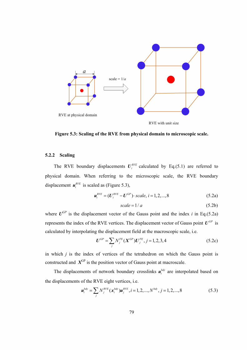
79

Figure 5.3: Scaling of the RVE from physical domain to microscopic scale.

5.2.2 Scaling

The RVE boundary displacements RVEiU calculated by Eq.(5.1) are referred to

physical domain. When referring to the microscopic scale, the RVE boundary

displacement RVEiu is scaled as (Figure 5.3),

( ) , 1, 2,...,8RVE RVE GPi i scale i u U U (5.2a)

1/scale a (5.2b)

where UGP is the displacement vector of the Gauss point and the index i in Eq.(5.2a)

represents the index of the RVE vertices. The displacement vector of Gauss point GPU is

calculated by interpolating the displacement field at the macroscopic scale, i.e.

( ) , 1, 2,3,4GP FE GP FE

j jj

N j U X U (5.2c)

in which j is the index of vertices of the tetrahedron on which the Gauss point is

constructed and XGP is the position vector of Gauss point at macroscale.

The displacements of network boundary crosslinks bdyiu are interpolated based on

the displacements of the RVE eight vertices, i.e.

( ) , 1, 2,..., , 1, 2,...,8bdy RVE bdy RVE bdy

i j i jj

N i N j u x u

(5.3)

80

where bdyjx is the position vector of boundary crosslink j, Nbdy is the total number of fiber

boundary crosslinks and NjRVE is the shape function of the cube.

5.2.3 Upscaling

After the RVE boundary value problem is solved, the average Cauchy stress

(Eq.5.9) and force balance (Eq.5.10) are returned to the macroscale to formulate

nonlinear finite element equations. The detailed nonlinear finite element formulation is

provided in section 5 of Appendix A.

5.3 Governing equations

Three governing equations are required to formulate the multiscale model: a

constitutive equation describing the force-elongation for the individual fiber; an equation

relating microscopic Cauchy stress to the volume-averaged Cauchy stress at

macroscopic scale and the equation for macroscopic stress balance [48].

Constitutive equation of individual fibers

( 1)ffib BE A

f eB

(5.4)

Parameters in Eq.(5.4) have the same definition as in Eq.(3.1).

Volume-averaged Cauchy stress at macroscale

The volume-averaged Cauchy stress tensor, ˆij at macroscopic scale is obtained

from the microscopic stress tensor ij by

, ,

,

1 1ij ij i ij k j k

V V Vi

dV dV u n dV V

(5.5)

where V is the volume of the representative volume element (RVE).

By multiplying microscopic stress ij with Kronecker delta δik,

,ij kj ik kj i kx

(5.6)

where xi is the ith component of position vector. Substituting Eq.(5.6) into Eq.(5.5) and

applying the divergence theorem to transform the volume integral into surface integral,

, ,

1 1 1ˆij kj i k kj i k kj k i

V V V

x dV x n d x dVV V V

(5.7)

81

Applying the microscopic equilibrium, i.e. , 0kj k and j kj kt n ,

1 1îj kj i k i j

V V

x n d x t dV V

(5.8)

where tj is the traction exerted on the boundaries of RVE. For a RVE consisting of only

fibers, Eq.(5.8) is written as

1îj i j

boundarynodes

x fV

(5.9)

where fj is the reaction force developed on the boundary node (crosslink) in j-direction.

This equation could also be written in the virial formula, i.e

all nodes

1îj i jx f

V

(5.10)

which also holds because, since the internal nodes are in equilibrium, the terms

corresponding to internal nodes do not contribute to the sum. Hence this sum is identical

to that in Eq. (5.9).

Force balance for the macroscopic scale

The momentum conservation equation at the macroscopic scale is derived by taking

derivative with respect to xi on both sides of Eq.(5.5) [65],

,, ,

1 1 1ij ij ij

iV V Vi i

dV dV dVV V V

(5.11)

Using Leibnitz’s rule, the first term on the right hand size of Eq.(5.11) is written as

, ,

,

1 1ij ij i ij k i k

V V Vi

dV dV u n dV V

(5.12)

Again, applying Leibnitz’s rule to the second term, we get

, , ,2

,

ˆ ˆ1 1( )ij ij

ij i ij i k i ki V V V V

dV V dV dV u n dV V V V

(5.13)

Combing Eq.(5.12) and (5.13) and noting the microscopic balance (i.e. , 0ij i ), the

conservation of momentum at macroscopic scale is obtained

,

,

ˆ 0

1ˆ( )

ij i j

j ij ij k i k

V

Q

Q u n dV

(5.14)

82

where uk is the displacement of the RVE boundary and nk is the unit normal vector. The

right hand side of Eq.(5.14) is due to the correlation between inhomogeneous

displacement of RVE boundary and local inhomogeneities in the stress field. The

macroscopic momentum balance equation given by Eq.(5.14) is solved by using finite

element analysis.

5.4 Relating the microscopic scale to the macroscopic scale

In the volume-averaged multiscale model, the RVE is assumed to represent a

material volume (a cube with side length a) at macroscale. The RVE scale is

dimensionless and the side is of unit length in the undeformed configuration. This

section reviews the conversion of the averaged stress calculated at the RVE scale to the

physical scale [48].

At the RVE scale, the total fiber length in the RVE (1*1*1 cube) is L

(dimensionless). Hence, the total fiber length in the macroscopic scale will be L·a and

the volume of fibers will be A·L·a. Therefore the volume fraction of fibers is

0 3 2

ALa AL

a a

(5.15)

Solving a from Eq.(5.15),

0

LAa

(5.16)

Therefore, the RVE side length at physical domain is determined by the fiber radius and

the volume fraction of the tissue. For the example shown in section 5.5, a is around

0.021mm.

Hence, the dimensional averaged stress 'ˆ ij is calculated as

' '

' 3 2

1 1 1ˆij i j i j i j

boundary boundary boundarynodes nodes nodes

x f ax f x fV Va Va

(5.17)

Substituting Eq.(5.16) into (5.17), the average Cauchy stress after conversion is

' 0ˆ ˆij ijLA

(5.18)

83

5.5 Example

A dogbone (shown in Figure 5.4) under 10% stretch is solved using the volume-

averaging based multiscale model. The problem is solved in 5 load steps with 2%

extension per step. The parameters in Eq.(5.4) are chosen as B=1.0, Ef=90Mpa,

A=7.854E-09mm2 corresponding to fiber radius 50nm, based on [66].

1x

2x3x

1 1 1

2 2 2

3 3 3

[ , ]

[ , ]

[ , ]

x x x

x x x

x x x

1 1 1

1 1 2

1 1 3

, 0

, 0

, 0

x x u

x x u

x x u

1 1 1 0

1 1 2

1 1 3

,

, 0

, 0

x x u u

x x u

x x u

Figure 5.4: (a) Dimensions of the sample considered in this example and (b) Boundary conditions.

(a)

(b)

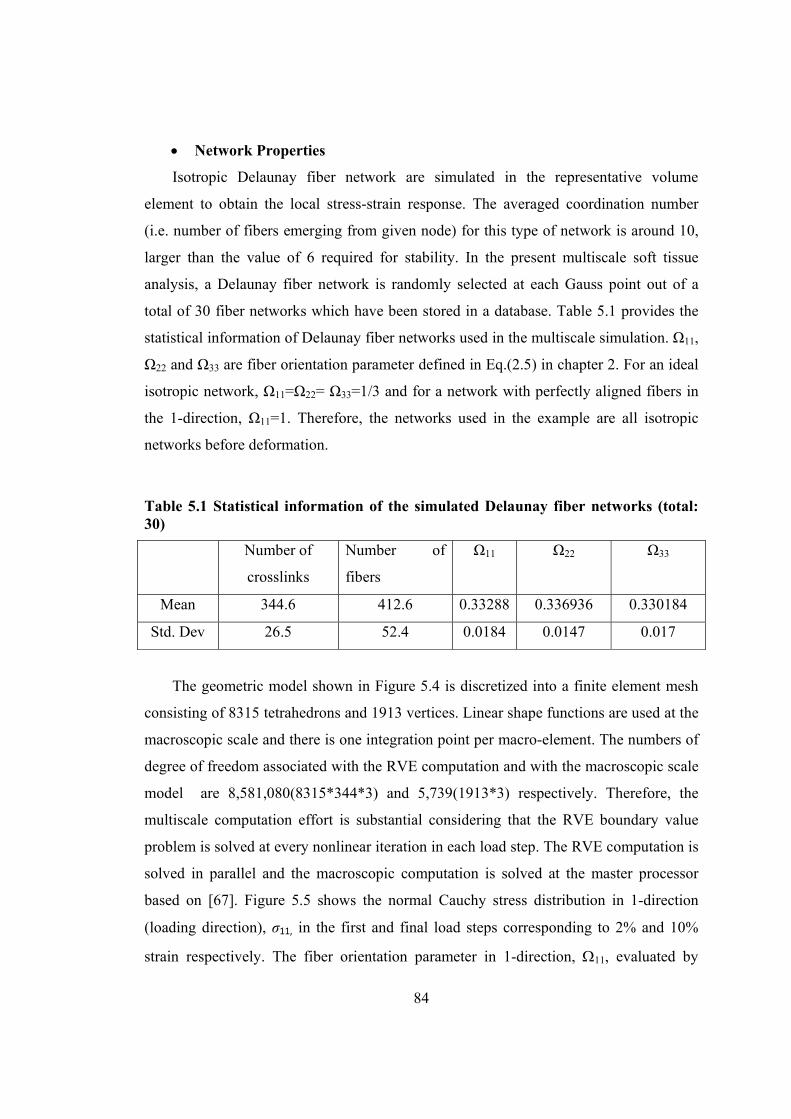
84

Network Properties

Isotropic Delaunay fiber network are simulated in the representative volume

element to obtain the local stress-strain response. The averaged coordination number

(i.e. number of fibers emerging from given node) for this type of network is around 10,

larger than the value of 6 required for stability. In the present multiscale soft tissue

analysis, a Delaunay fiber network is randomly selected at each Gauss point out of a

total of 30 fiber networks which have been stored in a database. Table 5.1 provides the

statistical information of Delaunay fiber networks used in the multiscale simulation. Ω11,

Ω22 and Ω33 are fiber orientation parameter defined in Eq.(2.5) in chapter 2. For an ideal

isotropic network, Ω11=Ω22= Ω33=1/3 and for a network with perfectly aligned fibers in

the 1-direction, Ω11=1. Therefore, the networks used in the example are all isotropic

networks before deformation.

Table 5.1 Statistical information of the simulated Delaunay fiber networks (total: 30)

Number of

crosslinks

Number of

fibers

Ω11 Ω22 Ω33

Mean 344.6 412.6 0.33288 0.336936 0.330184

Std. Dev 26.5 52.4 0.0184 0.0147 0.017

The geometric model shown in Figure 5.4 is discretized into a finite element mesh

consisting of 8315 tetrahedrons and 1913 vertices. Linear shape functions are used at the

macroscopic scale and there is one integration point per macro-element. The numbers of

degree of freedom associated with the RVE computation and with the macroscopic scale

model are 8,581,080(8315*344*3) and 5,739(1913*3) respectively. Therefore, the

multiscale computation effort is substantial considering that the RVE boundary value

problem is solved at every nonlinear iteration in each load step. The RVE computation is

solved in parallel and the macroscopic computation is solved at the master processor

based on [67]. Figure 5.5 shows the normal Cauchy stress distribution in 1-direction

(loading direction), σ11, in the first and final load steps corresponding to 2% and 10%

strain respectively. The fiber orientation parameter in 1-direction, 11, evaluated by

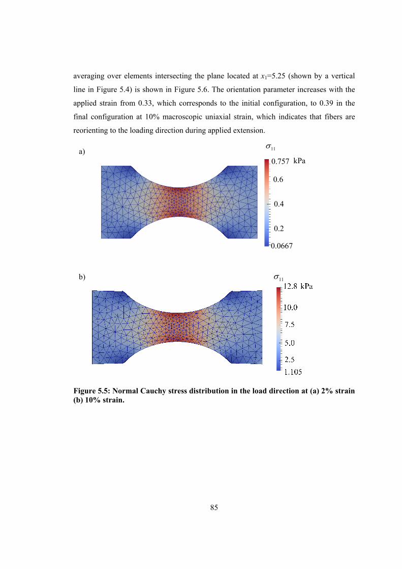
85

averaging over elements intersecting the plane located at x1=5.25 (shown by a vertical

line in Figure 5.4) is shown in Figure 5.6. The orientation parameter increases with the

applied strain from 0.33, which corresponds to the initial configuration, to 0.39 in the

final configuration at 10% macroscopic uniaxial strain, which indicates that fibers are

reorienting to the loading direction during applied extension.

0.0667

0.2

0.4

0.6

0.757 kPa

11

11

Figure 5.5: Normal Cauchy stress distribution in the load direction at (a) 2% strain (b) 10% strain.

a)

b)

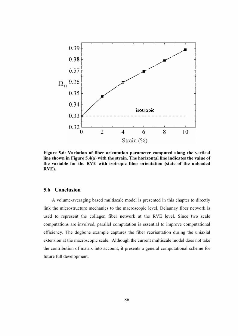
86

11

Figure 5.6: Variation of fiber orientation parameter computed along the vertical line shown in Figure 5.4(a) with the strain. The horizontal line indicates the value of the variable for the RVE with isotropic fiber orientation (state of the unloaded RVE).

5.6 Conclusion

A volume-averaging based multiscale model is presented in this chapter to directly

link the microstructure mechanics to the macroscopic level. Delaunay fiber network is

used to represent the collagen fiber network at the RVE level. Since two scale

computations are involved, parallel computation is essential to improve computational

efficiency. The dogbone example captures the fiber reorientation during the uniaxial

extension at the macroscopic scale. Although the current multiscale model does not take

the contribution of matrix into account, it presents a general computational scheme for

future full development.

87

6. Conclusion and future work

6.1 Conclusion

The mechanical behavior of a three-dimensional cross-linked fiber network

embedded in matrix is studied in this work. A finite element based coupled fiber-matrix

model was developed to quantify the internal stress field and to explore interactions

between the embedded fiber network and matrix.

In Chapter 2, we discussed the pre-processing step of the coupled fiber-matrix

model, i.e. the non-manifold geometry creation for the model of the fiber network

embedded in matrix, and multidimensional mesh generation. The geometry is based on a

full representation of the network, which is generated using a Voronoi tessellation. The

embedded fibers are represented as one-dimensional wire edges, therefore a non-

manifold geometric topological representation is required. Topological adjacencies

between geometric entities are specified by using Parasolid to create the non-manifold

geometry. The multi-dimensional mesh with fibers meshed into one-dimensional mesh

edges and matrix meshed into three-dimensional tetrahedrons are derived from the

created non-manifold geometry. Both isotropic and gradedmeshes are generated for

different purposes of finite element analysis. These developments make possible the

creation of complex models of various types of networks embedded in matrix.

In Chapter 3, the formulation of the nonlinear equations representing the coupled

fiber-matrix system was presented. Both geometric and material nonlinearities are taken

into account in the analysis. Individual fibers are modeled as nonlinear trusses and the

matrix material is modeled as compressible neo-Hookean material. The Newton’s

method is employed to solve the nonlinear equations and the tangential stiffness matrix

and force vector are derived for the coupled fiber-matrix system. These developments

make possible obtaining the non-linear solution for the models created using the

methods presented in Chapter 2.

In Chapter 4, the mechanical behavior of the RVE composite under tensile loading

was investigated by applying the coupled fiber-matrix model. In the nonlinear material

constitutive model where individual fibers are represented as nonlinear trusses and the

matrix is represented as neo-hookean material, anisotropic fiber networks are considered

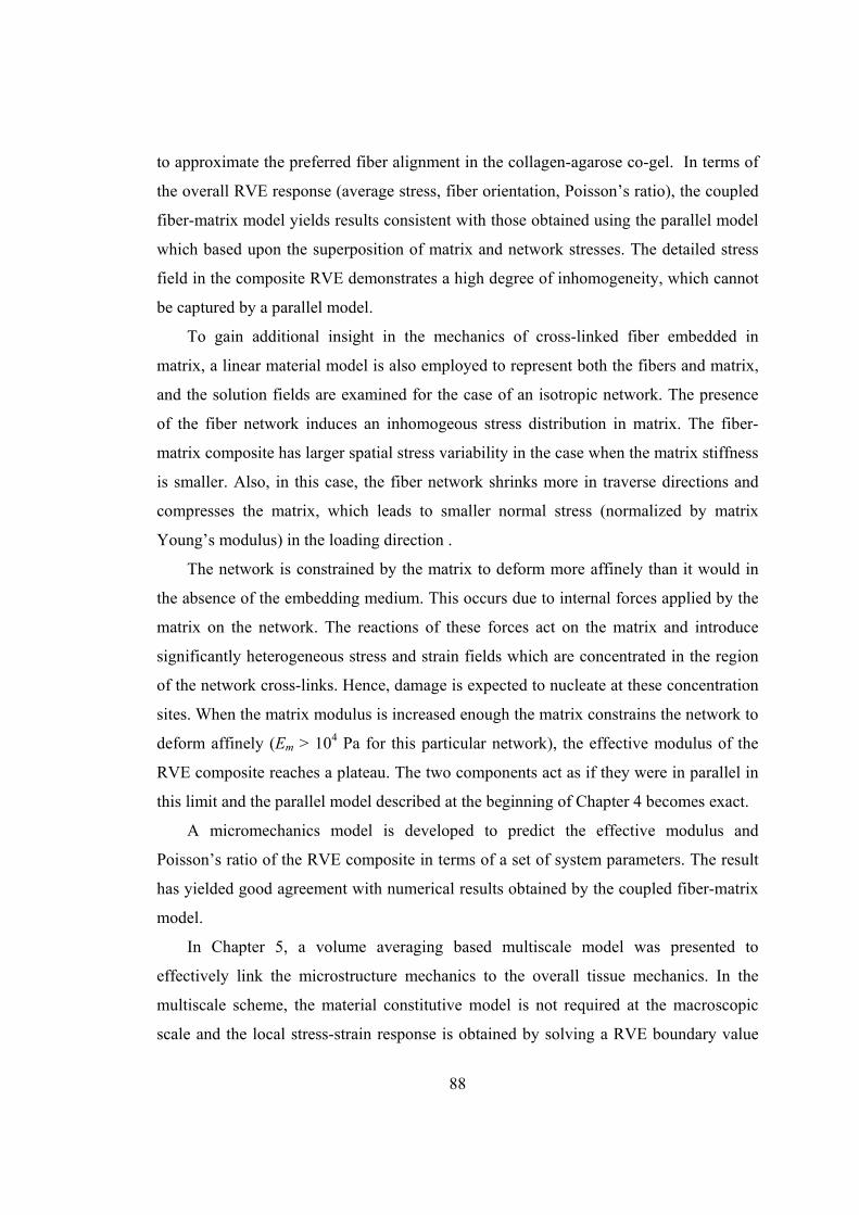
88

to approximate the preferred fiber alignment in the collagen-agarose co-gel. In terms of

the overall RVE response (average stress, fiber orientation, Poisson’s ratio), the coupled

fiber-matrix model yields results consistent with those obtained using the parallel model

which based upon the superposition of matrix and network stresses. The detailed stress

field in the composite RVE demonstrates a high degree of inhomogeneity, which cannot

be captured by a parallel model.


matrix, a linear material model is also employed to represent both the fibers and matrix,

and the solution fields are examined for the case of an isotropic network. The presence

of the fiber network induces an inhomogeous stress distribution in matrix. The fiber-

matrix composite has larger spatial stress variability in the case when the matrix stiffness

is smaller. Also, in this case, the fiber network shrinks more in traverse directions and

compresses the matrix, which leads to smaller normal stress (normalized by matrix

Young’s modulus) in the loading direction .

The network is constrained by the matrix to deform more affinely than it would in

the absence of the embedding medium. This occurs due to internal forces applied by the

matrix on the network. The reactions of these forces act on the matrix and introduce

significantly heterogeneous stress and strain fields which are concentrated in the region

of the network cross-links. Hence, damage is expected to nucleate at these concentration

sites. When the matrix modulus is increased enough the matrix constrains the network to

deform affinely (Em > 104 Pa for this particular network), the effective modulus of the

RVE composite reaches a plateau. The two components act as if they were in parallel in

this limit and the parallel model described at the beginning of Chapter 4 becomes exact.

A micromechanics model is developed to predict the effective modulus and

Poisson’s ratio of the RVE composite in terms of a set of system parameters. The result

has yielded good agreement with numerical results obtained by the coupled fiber-matrix

model.

In Chapter 5, a volume averaging based multiscale model was presented to

effectively link the microstructure mechanics to the overall tissue mechanics. In the

multiscale scheme, the material constitutive model is not required at the macroscopic

scale and the local stress-strain response is obtained by solving a RVE boundary value

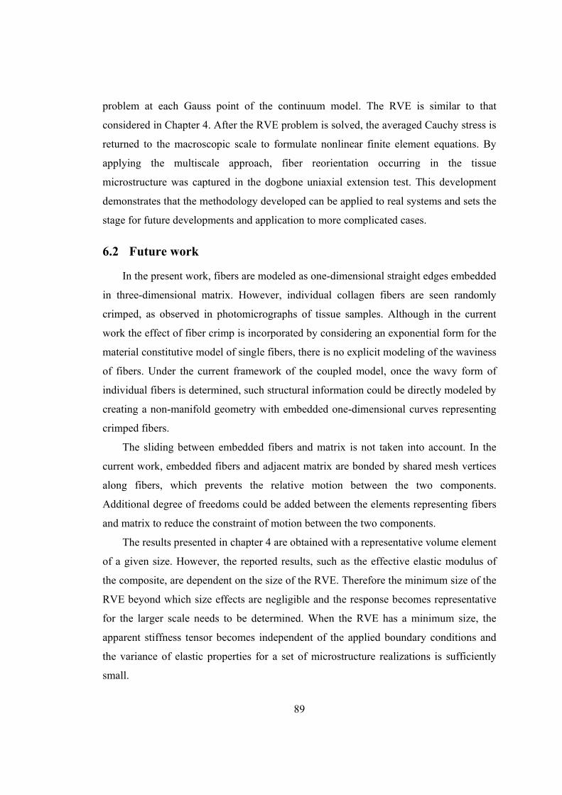
89

problem at each Gauss point of the continuum model. The RVE is similar to that

considered in Chapter 4. After the RVE problem is solved, the averaged Cauchy stress is

returned to the macroscopic scale to formulate nonlinear finite element equations. By

applying the multiscale approach, fiber reorientation occurring in the tissue

microstructure was captured in the dogbone uniaxial extension test. This development

demonstrates that the methodology developed can be applied to real systems and sets the

stage for future developments and application to more complicated cases.

6.2 Future work

In the present work, fibers are modeled as one-dimensional straight edges embedded

in three-dimensional matrix. However, individual collagen fibers are seen randomly

crimped, as observed in photomicrographs of tissue samples. Although in the current

work the effect of fiber crimp is incorporated by considering an exponential form for the

material constitutive model of single fibers, there is no explicit modeling of the waviness

of fibers. Under the current framework of the coupled model, once the wavy form of

individual fibers is determined, such structural information could be directly modeled by

creating a non-manifold geometry with embedded one-dimensional curves representing

crimped fibers.

The sliding between embedded fibers and matrix is not taken into account. In the

current work, embedded fibers and adjacent matrix are bonded by shared mesh vertices

along fibers, which prevents the relative motion between the two components.

Additional degree of freedoms could be added between the elements representing fibers

and matrix to reduce the constraint of motion between the two components.

The results presented in chapter 4 are obtained with a representative volume element

of a given size. However, the reported results, such as the effective elastic modulus of

the composite, are dependent on the size of the RVE. Therefore the minimum size of the

RVE beyond which size effects are negligible and the response becomes representative

for the larger scale needs to be determined. When the RVE has a minimum size, the

apparent stiffness tensor becomes independent of the applied boundary conditions and

the variance of elastic properties for a set of microstructure realizations is sufficiently

small.

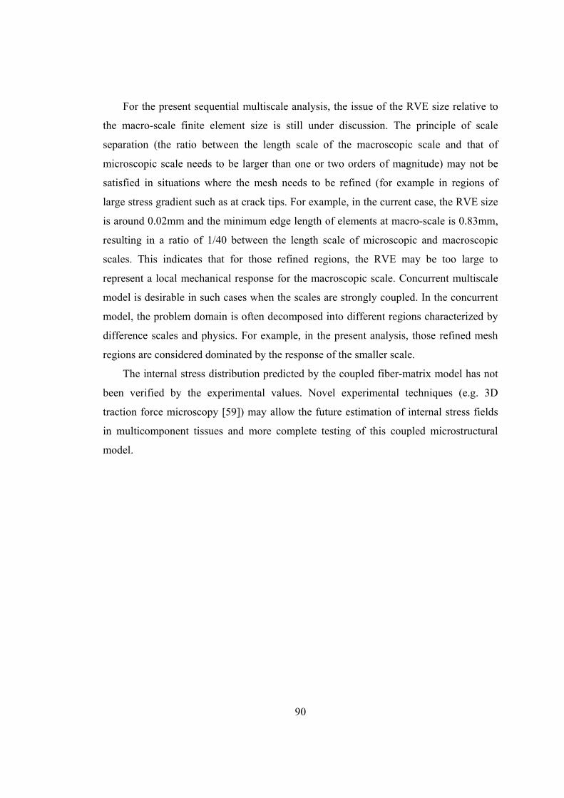
90

For the present sequential multiscale analysis, the issue of the RVE size relative to

the macro-scale finite element size is still under discussion. The principle of scale

separation (the ratio between the length scale of the macroscopic scale and that of

microscopic scale needs to be larger than one or two orders of magnitude) may not be

satisfied in situations where the mesh needs to be refined (for example in regions of

large stress gradient such as at crack tips. For example, in the current case, the RVE size

is around 0.02mm and the minimum edge length of elements at macro-scale is 0.83mm,

resulting in a ratio of 1/40 between the length scale of microscopic and macroscopic

scales. This indicates that for those refined regions, the RVE may be too large to

represent a local mechanical response for the macroscopic scale. Concurrent multiscale

model is desirable in such cases when the scales are strongly coupled. In the concurrent

model, the problem domain is often decomposed into different regions characterized by

difference scales and physics. For example, in the present analysis, those refined mesh

regions are considered dominated by the response of the smaller scale.

The internal stress distribution predicted by the coupled fiber-matrix model has not

been verified by the experimental values. Novel experimental techniques (e.g. 3D

traction force microscopy [59]) may allow the future estimation of internal stress fields

in multicomponent tissues and more complete testing of this coupled microstructural

model.

91

7. Reference

[1] D. L. Butler, S. A. Goldstein, R. E. Guldberg, X. E. Guo, R. Kamm, C. T. Laurencin, L. V. McIntire, V. C. Mow, R. M. Nerem, R. L. Sah, L. J. Soslowsky, R. L. Spilker, and R. T. Tranquillo, “The impact of biomechanics in tissue engineering and regenerative medicine,” Tissue Eng., vol. 15, p. 477, Dec. 2009.

[2] D. L. Butler, S. A. Goldstein, and F. Guilak, “Functional tissue engineering: The role of biomechanics,” J. Biomech. Eng., vol. 122, p. 570, Dec. 2000.

[3] U. A. Stock and J. P. Vacanti, “Tissue engineering: Current state and prospects,” Annu. Rev. Med., vol. 52, p. 443, Feb. 2001.

[4] J. Lemaitre, Handbook of Materials Behavior Models: Nonlinear Models and Properties, 2nd ed. San Diego, CA: Academic Press, 2001.

[5] S. P. Lake and V. H. Barocas, “Mechanical and structural contribution of non-fibrillar matrix in uniaxial tension: A collagen-agarose co-gel model.,” Ann. Biomed. Eng., vol. 39, p. 1891, Jul. 2011.

[6] J. D. Humphrey, “Continuum biomechanics of soft biological tissues,” Proc. R. Soc. London. Ser. A, vol. 459, p. 3, Jan. 2003.

[7] Y. C. Fung, “Elasticity of soft tissues in simple elongation,” Am. J. Physiol., vol. 213, p. 1532, Dec. 1967.

[8] J. D. Humphrey, R. K. Strumpf, and F. C. Yin, “Determination of a constitutive relation for passive myocardium: II. Parameter estimation,” J. Biomech. Eng., vol. 112, p. 340, Aug. 1990.

[9] C. O. Horgan and G. Saccomandi, “A description of arterial wall mechanics using limiting chain extensibility constitutive models,” Biomech. Model. Mechanobiol., vol. 1, p. 251, Apr. 2003.

[10] J. D. Humphrey, “Mechanics of the arterial wall: Review and directions,” Crit. Rev. Biomed. Eng., vol. 23, p. 1, Jan. 1995.

[11] Y. Lanir, “A structural theory for the homogeneous biaxial stress-strain relationships in flat collagenous tissues,” J. Biomech., vol. 12, p. 423, Jun. 1979.

[12] W. F. Decraemer, M. A. Maes, and V. J. Vanhuyse, “An elastic stress-strain relation for soft biological tissues based on a structural model,” J. Biomech., vol. 13, p. 463, Jun. 1980.

92

[13] M. S. Sacks, “Incorporation of experimentally-derived fiber orientation into a structural constitutive model for planar collagenous iissues,” J. Biomech. Eng., vol. 125, p. 280, Apr. 2003.

[14] D. H. Cortes, S. P. Lake, J. A. Kadlowec, L. J. Soslowsky, and D. M. Elliott, “Characterizing the mechanical contribution of fiber angular distribution in connective tissue: Comparison of two modeling approaches,” Biomech. Model. Mechanobiol., vol. 9, p. 651, Oct. 2010.

[15] H. P. Wagner and J. D. Humphrey, “Differential passive and active biaxial mechanical behaviors of muscular and elastic arteries: Basilar versus common carotid,” J. Biomech. Eng., vol. 133, p. 051009, May 2011.

[16] Y. Hollander, D. Durban, X. Lu, G. S. Kassab, and Y. Lanir, “Experimentally validated microstructural 3D constitutive model of coronary arterial media,” J. Biomech. Eng., vol. 133, p. 031007, Mar. 2011.

[17] P. H. Kao, S. R. Lammers, L. Tian, K. Hunter, K. R. Stenmark, R. Shandas, and H. J. Qi, “A microstructurally driven model for pulmonary artery tissue.,” J. Biomech. Eng., vol. 133, p. 051002, May 2011.

[18] A. L. F. Soares, M. Stekelenburg, and F. P. T. Baaijens, “Remodeling of the collagen fiber architecture due to compaction in small vessels under tissue engineered conditions,” J. Biomech. Eng., vol. 133, p. 071002, Jul. 2011.

[19] N. T. Jacobs, D. H. Cortes, E. J. Vresilovic, and D. M. Elliott, “Biaxial tension of fibrous tissue: Using finite element methods to address experimental challenges arising from boundary conditions and anisotropy,” J. Biomech. Eng., vol. 135, p. 021004, Feb. 2013.

[20] G. A. Ateshian, V. Rajan, N. O. Chahine, C. E. Canal, and C. T. Hung, “Modeling the matrix of articular cartilage using a continuous fiber angular distribution predicts many observed phenomena,” J. Biomech. Eng., vol. 131, p. 061003, Jun. 2009.

[21] T. C. Gasser, R. W. Ogden, and G. A. Holzapfel, “Hyperelastic modelling of arterial layers with distributed collagen fibre orientations,” J. R. Soc. Interface, vol. 3, p. 15, Mar. 2006.

[22] A. D. Freed, D. R. Einstein, and I. Vesely, “Invariant formulation for dispersed transverse isotropy in aortic heart valves: An efficient means for modeling fiber splay,” Biomech. Model. Mechanobiol., vol. 4, p. 100, Nov. 2005.

[23] R. C. Picu, “Mechanics of random fiber networks—a review,” Soft Matter, vol. 7, p. 6768, May 2011.

93

[24] K. L. Billiar, M. S. Sacks, and C. Gables, “A method to quantify the fiber kinematics of planar tissues under biaxial stretch,” J. Biomech., vol. 30, p. 753, Jul. 1997.

[25] K. K. Brewer, H. Sakai, A. M. Alencar, A. Majumdar, S. P. Arold, K. R. Lutchen, E. P. Ingenito, and B. Suki, “Lung and alveolar wall elastic and hysteretic behavior in rats: Effects of in vivo elastase treatment,” J. Appl. Physiol., vol. 95, p. 1926, Nov. 2003.

[26] P. L. Chandran and V. H. Barocas, “Affine versus non-affine fibril kinematics in collagen networks: Theoretical studies of network behavior,” J. Biomech. Eng., vol. 128, p. 259, Apr. 2006.

[27] D. A. Head, A. J. Levine, and F. C. MacKintosh, “Deformation of cross-linked semiflexible polymer networks,” Phys. Rev. Lett., vol. 91, p. 108102, Sep. 2003.

[28] D. A. Head, A. J. Levine, and F. C. MacKintosh, “Distinct regimes of elastic response and deformation modes of cross-linked cytoskeletal and semiflexible polymer networks,” Phys. Rev. E, vol. 68, p. 061907, Dec. 2003.

[29] H. Hatami-Marbini and R. C. Picu, “Scaling of nonaffine deformation in random semiflexible fiber networks,” Phys. Rev. E, vol. 77, p. 062103, Jun. 2008.

[30] P. R. Onck, T. Koeman, T. van Dillen, and E. van der Giessen, “Alternative explanation of stiffening in cross-linked semiflexible networks,” Phys. Rev. Lett., vol. 95, p. 178102, Oct. 2005.

[31] J. Liu, G. H. Koenderink, K. E. Kasza, F. C. MacKintosh, and D. A. Weitz, “Visualizing the strain field in semiflexible polymer networks: Strain fluctuations and nonlinear rheology of f-actin gels,” Phys. Rev. Lett., vol. 98, p. 198304, May 2007.

[32] F. LeonForte, A. Tanguy, J. P. Wittmer, and J. L. Barrat, “Continuum limit of amorphous elastic bodies II: Linear response to a point source force,” Phys. Rev. B, vol. 70, p. 014203, Jul. 2004.

[33] B. A. DiDonna and T. C. Lubensky, “Nonaffine correlations in random elastic media,” Phys. Rev. E, vol. 72, p. 066619, Dec. 2005.

[34] G. A. Holzapfel, T. C. Gasser, and R. W. Ogden, “A new constitutive framework for arterial wall mechanics and a comparative study of material models,” J. Elast., vol. 61, p. 1, Jul. 2000.

[35] N. J. B. Driessen, C. V. C. Bouten, and F. P. T. Baaijens, “A Structural Constitutive Model For Collagenous Cardiovascular Tissues Incorporating the Angular Fiber Distribution,” J. Biomech. Eng., vol. 127, p. 494, Jun. 2005.

94

[36] H. Tang, M. J. Buehler, and B. Moran, “A constitutive model of soft tissue: From nanoscale collagen to tissue continuum,” Ann. Biomed. Eng., vol. 37, p. 1117, Jun. 2009.

[37] T. Nagel and D. J. Kelly, “Remodelling of collagen fibre transition stretch and angular distribution in soft biological tissues and cell-seeded hydrogels.,” Biomech. Model. Mechanobiol., vol. 11, p. 325, Mar. 2012.

[38] K. M. Quapp and J. A. Weiss, “Material characterization of human medial collateral ligament,” J. Biomech. Eng., vol. 120, p. 757, Dec. 1998.

[39] H. L. Guerin and D. M. Elliott, “Quantifying the contributions of structure to annulus fibrosus mechanical function using a nonlinear, anisotropic, hyperelastic model,” J. Orthop. Res., vol. 24, p. 508, Apr. 2007.

[40] A. C. Abraham, J. T. Moyer, D. F. Villegas, G. M. Odegard, and T. L. Haut Donahue, “Hyperelastic properties of human meniscal attachments,” J. Biomech., vol. 44, p. 413, Feb. 2011.

[41] D. H. Cortes and D. M. Elliott, “Extra-fibrillar matrix mechanics of annulus fibrosus in tension and compression,” Biomech. Model. Mechanobiol., vol. 11, p. 781, Jul. 2012.

[42] D. R. Wagner and J. C. Lotz, “Theoretical model and experimental results for the nonlinear elastic behavior of human annulus fibrosus,” J. Orthop. Res., vol. 22, p. 901, Jul. 2004.

[43] X. Q. Peng, Z. Y. Guo, and B. Moran, “An anisotropic hyperelastic constitutive model with fiber-matrix shear interaction for the human annulus fibrosus,” J. Appl. Mech., vol. 73, p. 815, May 2005.

[44] G. D. O’Connell, H. L. Guerin, and D. M. Elliott, “Theoretical and uniaxial experimental evaluation of human annulus fibrosus degeneration,” J. Biomech. Eng., vol. 131, p. 111007, Nov. 2009.

[45] S. P. Lake, M. F. Hadi, V. K. Lai, and V. H. Barocas, “Mechanics of a fiber network within a non-fibrillar matrix: Model and comparison with collagen-agarose co-gels,” Ann. Biomed. Eng., vol. 40, p. 2111, Oct. 2012.

[46] E. A. Sander, T. Stylianopoulos, R. T. Tranquillo, and V. H. Barocas, “Image-based multiscale modeling predicts tissue-level and network-level fiber reorganization in stretched cell-compacted collagen gels,” Proc. Natl. Acad. Sci. U. S. A., vol. 106, p. 17675, Oct. 2009.

95

[47] S. Nachtrab, S. C. Kapfer, C. H. Arns, M. Madadi, K. Mecke, and G. E. Schröder-Turk, “Morphology and linear-elastic moduli of random network solids,” Adv. Mater., vol. 23, p. 2633, Jun. 2011.

[48] T. Stylianopoulos and V. H. Barocas, “Volume-averaging theory for the study of the mechanics of collagen networks,” Comput. Methods Appl. Mech. Eng., vol. 196, p. 2981, Jun. 2007.

[49] K. J. Weiler, Topological structures for geometric modeling. Ph.D dissertation, Dept. Comput. Sci., Rensselaer Polytechnic Institute, Troy, NY, 1986.

[50] Siemens Product Lifecycle Management Software, Inc., “Parasolid.” [Online]. Available: http:www.plm.automation.siemens.com/, [Accessed Dec. 6. 2013].

[51] Simmetrix Inc., “The simulation modeling suite.” [Online]. Available: http://www.simmetrix.com/, [Accessed Dec. 6. 2013].

[52] L. Zhang, S. P. Lake, V. K. Lai, C. R. Picu, V. H. Barocas, and M. S. Shephard, “A coupled fiber-matrix model demonstrates highly inhomogeneous microstructural interactions in soft tissues under tensile load,” J. Biomech. Eng., vol. 135, p. 011008, Jan. 2013.

[53] G. A. Holzapfel, Nonlinear Solid Mechanics: A Continuum Approach for Engineering,1st ed. West Sussex, England: Wiley, 2000.

[54] K. J. Bathe, Finite Element Procedures, 1st ed. Upper Saddle River, New Jersey: Prentice Hall, 1996.

[55] P. Wriggers, Nonlinear Finite Element Methods, 1st ed. Hannover, Germany: Springer, 2008.

[56] T. Belytschko, W. K. Liu and B. Moran, Nonlinear Finite Elements for Continua and Structures, 1st ed. West Sussex, England: Wiley, 2000.

[57] A. F. Bower, Applied Mechanics of Solids, 1st ed. Boca Raton, Florida: CRC Press, 2009.

[58] L. Zhang, S. P. Lake, V. H. Barocas, M. S. Shephard, and R. C. Picu, “Cross-linked fiber network embedded in an elastic matrix,” Soft Matter, vol. 9, p. 6398, Jul. 2013.

[59] C. Franck, S. A. Maskarinec, D. A. Tirrell, and G. Ravichandran, “Three dimensional traction force microscopy: A new tool for quantifying cell-matrix interactions,” PLoS One, vol. 6, p. e17833, Mar. 2011.

96

[60] M. Kellomäki, J. Åström, and J. Timonen, “Rigidity and dynamics of random spring networks,” Phys. Rev. Lett., vol. 77, p. 2730, Sep. 1996.

[61] A. Shahsavari and R. C. Picu, “Model selection for athermal cross-linked fiber networks,” Phys. Rev. E, vol. 86, p. 011923, Jul. 2012.

[62] D. H. Lee and G. A. Carnaby, “Compressional energy of the random fiber assembly, part I: Theory,” Text. Res. J., vol. 62, p. 185, Apr. 1992.

[63] X. F. Wu and Y. A. Dzenis, “Elasticity of planar fiber networks,” J. Appl. Phys., vol. 98, p. 093501, Nov. 2005.

[64] A. E. H. Love, A Treatise on the Mathematical Theory of Elasticity, 4th ed. Mineola, New York: Dover, 2011.

[65] P. L. Chandran and V. H. Barocas, “Deterministic material-based averaging theory model of collagen gel micromechanics,” J. Biomech. Eng., vol. 129, p. 137, Apr. 2007.

[66] P. L. Chandran, T. Stylianopoulos, and V. H. Barocas, “Microstructure-based, multiscale modeling for the mechanical behavior of hydrated fiber networks,” Multiscale Model. Simul., vol. 7, p. 22, Apr. 2008.

[67] X. J. Luo, T. Stylianopoulos, V. H. Barocas, and M. S. Shephard, “Multiscale computation for bioartificial soft tissues with complex geometries,” Eng. Comput., vol. 25, p. 87, Sep. 2008.

97

Appendix A

Documentation on finite element code of multiscale soft tissue analysis 1. Flow chart of the multiscale code

The flow chart of the multiscale soft tissue computation is shown in Figure A.1,

which employs an incremental-iterative approach (details in Chapter 3.). The only

difference from the standard approach is that microscale computation is executed at each

nonlinear iteration before computing the tangential stiffness matrix and force vector at

the macroscale to provide averaged stress and stress derivative on each Gauss point. In

the following flow chart, the micro-scale computation is denoted as ‘compute RVEs’.

1i i u u u

Yes

No

YesNo

Figure A.1 flow chart of the multi-scale code

98

2. Interface functions passing information through scales

The multiscale analysis code consists of two scale computation. Each scale is

treated as a C++ object with carefully designed member functions. The macro-scale

computation is represented as class ‘NonLinTissue’; the micro-scale computation is

represented as class ‘RepresentVolElem’. The two scales communicate through

interfaces functions. Class definitions with essential member functions are provided in

section 4.

2.1 Interface functions related to macro-scale to micro-scale information passing

The information passed from macroscale to microscale includes the nodal

displacements of macro element on which the representative volume element (RVE) is

constructed.

Related interface functions are:

// Retrieve the nodal displacements of mesh entity ‘pEntity’ and write into an array of double

Void NonLinTissue :: retrieveCoordsDisp(pEntity, double *);

// Pass the nodal displacement of macro element to its RVE

void RepresentVolElem :: setupCoordsDisp(double *coordDisp);

2.2 Interface functions related to micro-scale to macro-scale information passing

The information passed from microscale to macroscale includes: (1) averaged stress

(2) body force (3) the derivative of averaged stress with respect to the nodal

displacement of macro element on which RVE is constructed.

Related interface functions are:

// Compute the averaged stress of the RVE and write it in the array ‘vstress’

void RepresentVolElem :: calc_stress(double fvec[],double vstress[], int pas);

// Compute the unbalanced body force (referred as Q term in Chapter 5)

void RepresentVolElem :: avgvolstress(double fvec[],double vstress[],double loc_vastrx[], double

loc_vastry[],double loc_vastrz[],double vol,double coords_loc[], int nfe, int pas,double

init_coords_loc[],double fem_res_norm);

99

// Compute the derivative of averaged stress with respect to nodal displacement of macro

element

void RepresentVolElem :: calc_femjacob_newmethod(double dSdx[],int pas,double vol,double

dvol[],double vstress[],int tag,double init_coords_loc[],int nfe,int iter,int nmesh);

// Retrieve the averaged stress, body force(Q term) and stress derivative from the RVE on mesh

entity pEntity;

SCOREC_Core::RVEInfo * NonLinTissue :: retrieveMatLawFromRVE (pEntity, int);

3. Pseudo code on the multiscale software design

The pseudo code for the mutilscale analysis is given below. In the pseudo code,

‘NLT’ represents the object with class type as ‘NonLinTissue’(macroscale); ‘RVE’

represents the object with class type ‘RepresentVolElem’(microscale). The first piece is

the main flow described in Figure 1; the second piece represents microscale

computation.

(1) Pseudo code of multiscale analysis

Input: geometry,mesh and attribute

// apply dirichlet boundary conditions

NLT->dirichlet();

// set up convergence tolerance

NLT->setConvTol();

Set current load step equal to 0

Set current nonlinear iteration equal to 0

Loop current load step = 0 to maximum load step

If current nonlinear iteration equal to 0

// set up and apply initial guess to the current displacement field

NLT-> SetInitialGuess();

Do

// retrieve the updated nodal displacement at each macro element to deform

RVE

NLT->retrieveCoordsDisp();

// compute all RVEs driven by macro deformation field

NLT->computeRVEs();

// retrieve averaged stress and stress derivative after RVE computation

NLT->retrieveMatLawFromRVE();

// compute the tangential matrix stiffness at macroscale

100

NLT->rveComputeTangentMatrix();

// compute the residual force vector at macroscale

NLT->rveComputeForceVector();

// solve the linear system to get incremental nodal displacement

NLT->solveLinearSystem();

// update the solution field

NLT->updateSolutionField();

// increase the index for nonlinear iteration

Current nonlinear iteration ++;

While (norm > tolerance)

Current load step ++;

End Loop

(2) Pseudo code of RVE computation

// retrieve nodal displacement at each macro element

NLT->retrieveCoordsDisp();

// pass nodal displacement of the macro element to RVE

RVE->setupCoordsDisp();

// Run RVE

RVE->run();

// calculate averaged stress

RVE->calculateAveragedStress();

// calculate the body force (Q term)

RVE->calculateBodyForceQterm();

// calculate the averaged stress derivative with respect to nodal displacement of macro element

RVE->calculateStressDerivative();

4. Class definitions for macro-scale and micro-scale

Class NonLinTissue : FiniteElementAnalysis Public: // Initialization void init(); // Apply dirichlet(essential) boundary condition virtual void dirichlet(); // Apply Neumann boundary condition

101

void neumann(); // Run the macroscale computation int run(bool); // Set the maximum number of nonlinear iteration void setNoOfIterations(int noiters); // Set the convergence tolerance void setConvTol(double convtol); // Set total number of load steps void setNumberOfLoadStep(int NbLoadStep); // Write the mesh after deformation in VTK format void writeToVTK(char *); Private: // Assemble tangential stiffness matrix and force vector void assembleSystem (const std::string &systemName = "Default"); // Compute residual force vector at macroscale void rveComputeForceVector(int, int, int, const std::string &, const FiniteElementAnalysis::TimeDerivative, const bool, const std::string &); // Compute tangential stiffness matrix at macroscale void rveComputeTangentMatrix(int, int, int, const std::string &, const FiniteElementAnalysis::TimeDerivative, const bool, const std::string &); // Compute element tangent stiffness matrix double * computeElementTangentStiffMatrix(pEntity, FiniteElementField*) ; // Compute element residual force vector double * computeElementForceVector(pEntity, FiniteElementField*) ; // Apply the initial guess to the current displacement field bool SetInitialGuess(); // Set up material parameter in the linear elasticity computation bool SetupLinElasticity(pGModel model, pMesh inMesh); // Run linear elasticity computation bool ComputeLinElasticity(); // Retrieve averaged stress and stress derivative on pEntity SCOREC_Core::RVEInfo * retrieveMatLawFromRVE(pEntity, int); // Execute microscale RVE computation on all macro elements void computeRVEs(FiniteElementField*); Class RepresentVolElem

102

Public: // pass initial coordinates of nodes of macro finite element to RVE void setupInitCoords(double *initCoords); // pass nodal displacement of the macro element to RVE void setupCoordsDisp(double *coordDisp); // run RVE computation void run(int iter =0); // Output the fiber configuration in VTK format void outputFiberToVTK(const char *); Private: // pointer to array of fiber nodes node_struct *arrnode; // pointer to array of fiber elements elmt_struct *arrelmt; // read in network information void read_init_net(char *finname,int pas); // calculate averaged stress, body force and stress derivative void calc_stress(double fvec[],double vstress[], int pas); void avgvolstress(double fvec[],double vstress[],double loc_vastrx[], double loc_vastry[],double loc_vastrz[],double vol,double coords_loc[], int nfe, int pas,double init_coords_loc[],double fem_res_norm); void calc_femjacob_newmethod(double dSdx[],int pas,double vol,double dvol[],double vstress[],int tag,double init_coords_loc[],int nfe,int iter,int nmesh); 5. Nonlinear finite element formulation

The principle of virtual displacement with incremental decomposition is

ij ij ij ij ij ij

V V V

dV dV R e dV

(A.1)

with

ij ij ije

(A.2)

, , , ,

1 1( ),

2 2ij i j j i ij k i k je u u u u (A.3)

i i

V

R Q u dV (A.4)

where ij and ij are incremental unknown stress and strain from last known state to

the known state , ij is the Cauchy stress at last known state which is returned as

averaged stress from the RVE constructed at the Gauss point, R is the virtual external

103

work done by Qi , which is the body force returned from the RVE constructed at the

Gauss point and u is incremental displacement from iteration i to iteration i+1.

Using Taylor’s series,

The first term in the left hand side of Eq.(A.1) is expanded as

ij ijk k kij ij l ij l ij ijkl l ijk k

l lV V V V

dV u dV u e dV C u e dVu u

(A.5)

ijijkl k

l

Cu

(A.6)

where klu is the component l of displacement vector at node k of the macro finite

element; ij

klu

is the derivative of the averaged stress (returned from RVE) with respect

to the nodal displacement of the macro finite element.

Substituting (A.5) into (A.1), Eq.(A.1) becomes

kijkl l ij ij ij i i ij ij

V V V V

C u e dV dV Q u dV e dV

(A.7)

Writing (A.7) into matrix form,

0( )

Tk T Tijkl l ij L LV

V

C u e dV dV u B C Δu u K Δu

(A.8a)

( )

TT Tij ij NL NL NLV

V

dV dV u B σB Δu u K Δu

(A.8b)

T T Ti i

V V

Q u dV dV u N Q u P

(A.8c)

0( )

TT Tij ij LV

V

e dV dV u B σ u F

(A.8d)

0( )

T TL NL

TT T TLV

V

dV dV

u K Δu u K Δu

u N Q u B σ

(A.8e)

( )L NL K K u P F (A.8f)

where

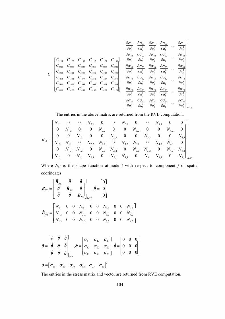
104

1111 1122 1133 1112 1123 1131

2211 2222 2233 2212 2223 2231

3311 3322 3333 3312 3323 3331

1211 1222 1233 1212 1223 1231

2311 2322 2333 2333 2323 2323

3111 3122 3133 3133 3123 3123

C C C C C C

C C C C C C

C C C C C CC

C C C C C C

C C C C C C

C C C C C C

11 11 11 11 111 1 1 2 41 2 3 1 3

22 22 22 22 221 1 1 2 41 2 3 1 3

33 33 33 33 331 1 1 2 41 2 3 1 3

12 12 12 12 121 1 1 2 41 2 3 1 3

23 23 231 1 11 2 3

...

...

...

...

u u u u u

u u u u u

u u u u u

u u u u u

u u u

23 232 41 3

31 31 31 31 311 1 1 2 41 2 3 1 3 6 12

...

...

u u

u u u u u

The entries in the above matrix are returned from the RVE computation.

1,1 2,1 3,1 4,1

1,2 2,2 3,2 4,2

1,3 2,3 3,3 4,30

1,2 1,1 2,2 2,1 3,2 3,1 4,2 4,1

1,3 1,2 2,3 2,2 3,3 3,2 4,3 4,2

1,3 1,1 2,3 2,1 3,3 3,1 4,3 4,1

0 0 0 0 0 0 0 0

0 0 0 0 0 0 0 0

0 0 0 0 0 0 0 0

0 0 0 0

0 0 0 0

0 0 0 0

L

N N N N

N N N N

N N N NB

N N N N N N N N

N N N N N N N N

N N N N N N N N

6 12

Where Ni,j is the shape function at node i with respect to component j of spatial

coorindates.

9 12

0

, 0

0NL

NL

NL

NL

B 0 0

B 0 B 0 0

0 0 B

1,1 2,1 3,1 4,1

1,2 2,2 3,2 4,2

1,3 2,3 3,2 4,3

0 0 0 0 0 0

0 0 0 0 0 0

0 0 0 0 0 0

N N N N

N N N N

N N N NNLB

11 12 13

12 22 23

13 23 339 9

ˆ ˆˆ 0 0 0ˆ ˆ ˆˆ ˆ, , 0 0 0

ˆ ˆ 0 0 0ˆ

σ 0 0

σ 0 σ 0 σ 0

0 0 σ

11 22 33 12 23 13

T σ

The entries in the stress matrix and vector are returned from RVE computation.

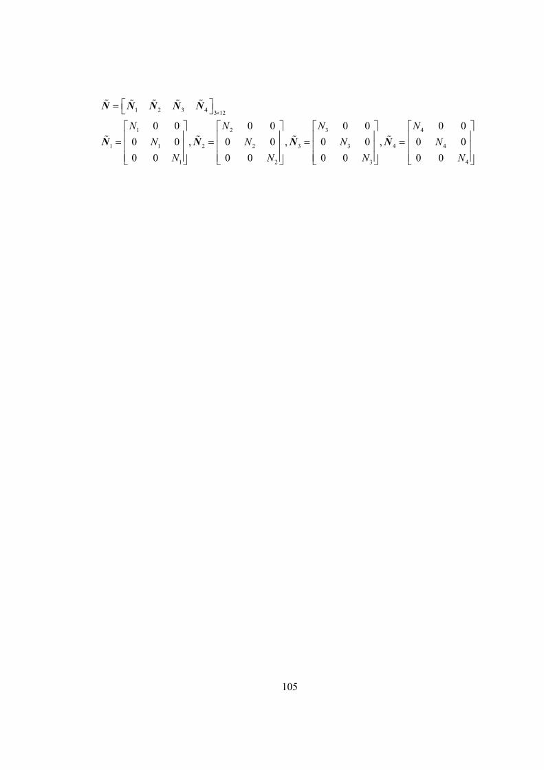
105

1 2 3 4 3 12

1 2 3 4

1 1 2 2 3 3 4 4

1 2 3 4

0 0 0 0 0 0 0 0

0 0 , 0 0 , 0 0 , 0 0

0 0 0 0 0 0 0 0

N N N N

N N N N

N N N N

N N N N N

N N N N

Microstructural modeling of cross-linked fiber network ... · Microstructural modeling of...

Documents

Transcript of Microstructural modeling of cross-linked fiber network ... · Microstructural modeling of...