Microstructural and mechanical properties of maraging ... · Microstructural and mechanical...
91
School of Industrial and Information Engineering Master Degree in Materials Engineering and Nanotechnology Microstructural and mechanical properties of maraging steel parts produced by selective laser melting Supervisor: Prof. Maurizio Vedani Co-Supervisor: Dr. Riccardo Casati Thesis work by: Carlo Masneri ID: 841632 Academic Year 2015/2016
Transcript of Microstructural and mechanical properties of maraging ... · Microstructural and mechanical...

School of Industrial and Information Engineering
Master Degree in Materials Engineering and Nanotechnology
Microstructural and mechanical properties of
maraging steel parts produced by selective laser
melting
Supervisor: Prof. Maurizio Vedani
Co-Supervisor: Dr. Riccardo Casati
Thesis work by:
Carlo Masneri
ID: 841632
Academic Year 2015/2016


I
TABLE OF CONTENTS
List of figures ................................................................................................................................ III
List of tables ................................................................................................................................. VI
Abstract ....................................................................................................................................... VII
Estratto ........................................................................................................................................ VII
1 Introduction .......................................................................................................................... 1
1.1 Selective laser melting .................................................................................................. 1
1.2 Maraging steel ............................................................................................................... 4
1.2.1 Precipitation strengthening................................................................................... 6
1.2.2 Precipitation in maraging steels ............................................................................ 9
1.2.3 Austenite reversion ............................................................................................. 11
2 Materials and methods ....................................................................................................... 13
2.1 Material ....................................................................................................................... 13
2.2 Processing methods .................................................................................................... 14
2.2.1 Selective laser melting ........................................................................................ 14
2.2.2 Heat treatment .................................................................................................... 15
2.3 Characterization methods ........................................................................................... 16
2.3.1 Optical microscopy .............................................................................................. 16
2.3.2 Scanning electron microscopy ............................................................................ 16
2.3.3 Stereoscope ......................................................................................................... 17
2.3.4 Differential scanning calorimetry ........................................................................ 18
2.3.5 Vickers micro-hardness ....................................................................................... 20
2.3.6 Tensile testing ..................................................................................................... 21
2.3.7 XRD analysis......................................................................................................... 22
3 Results and discussion ......................................................................................................... 24
3.1 As build and Solution treated samples comparison .................................................... 24
3.1.1 Microstructural characterization ........................................................................ 24
3.1.2 Kinetic analysis of ageing sequence .................................................................... 27
3.1.3 Ageing tests ......................................................................................................... 34
3.1.4 Tensile test .......................................................................................................... 36
3.2 As build samples characterization ............................................................................... 38

II
3.2.1 Ageing test ........................................................................................................... 38
3.2.2 Microstructural characterization of aged samples ............................................. 40
3.2.3 Tensile test .......................................................................................................... 46
3.2.4 Fracture analysis .................................................................................................. 49
3.3 Defects analysis ........................................................................................................... 52
3.3.1 Section analysis ................................................................................................... 52
3.3.2 Powder characterization ..................................................................................... 54
3.3.3 As built top surfaces analysis .............................................................................. 57
4 Conclusions ......................................................................................................................... 63
5 Appendix ............................................................................................................................. 67
5.1 Lattice microstructure ................................................................................................. 67
5.2 Ageing of AB and SOL samples at 460°C and 490°C .................................................... 68
5.3 Ageing of AB samples at 540°C and 600°C .................................................................. 69
5.4 Y and dY/dT vs. T curves for precipitation .................................................................. 70
5.5 Arrhenius and Kissinger plots for precipitation .......................................................... 71
5.6 Y and dY/dT vs. T curves for reversion ........................................................................ 72
5.7 Arrhenius and Kissinger plots for reversion ................................................................ 74
6 Bibliography ........................................................................................................................ 76
Ringraziamenti ............................................................................................................................ 81
III
LIST OF FIGURES
Figure 1. Schematic description of a SLM printer [2]. ................................................................... 2
Figure 2. Scheme of strengthening and softening contribution in maraging steels during aging
after solution treatment [18]. ....................................................................................................... 6
Figure 3. Comparison of a) growth and b) coarsening mechanisms [15]. .................................... 7
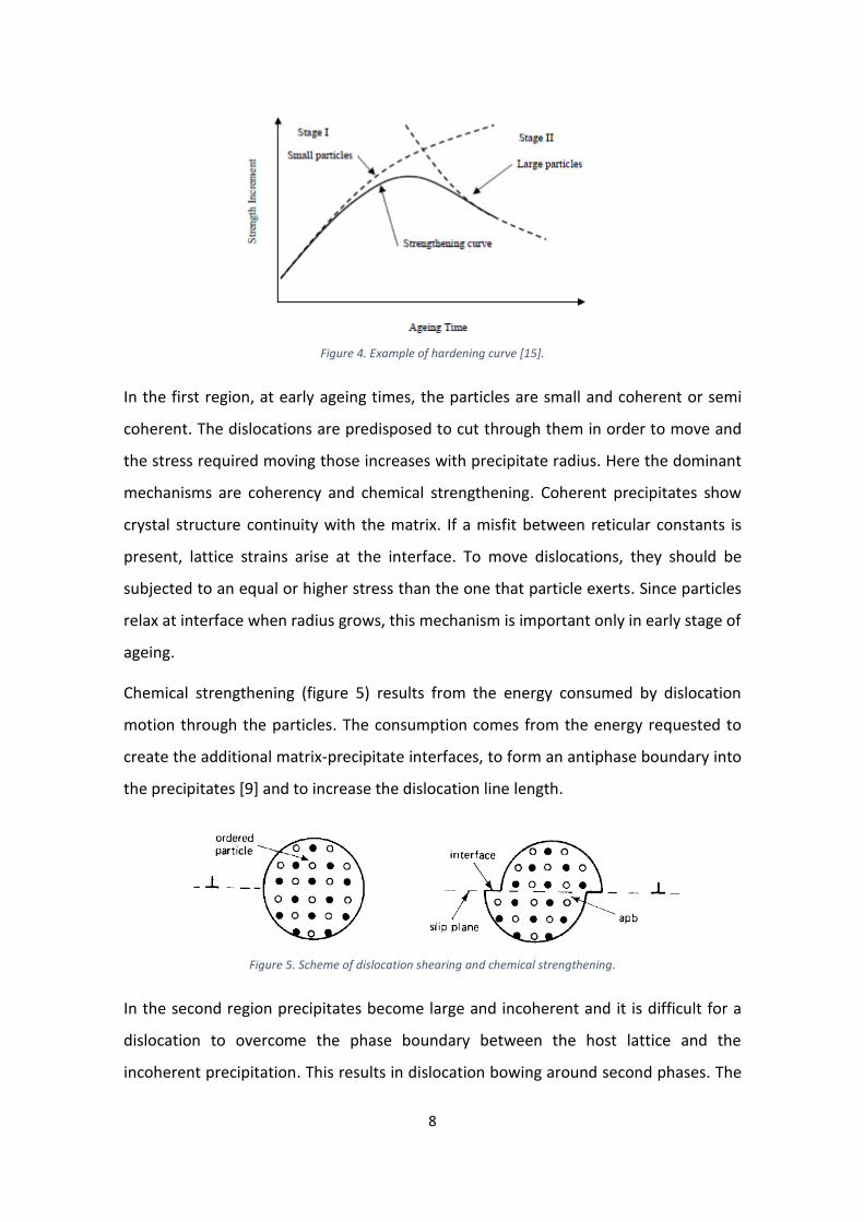
Figure 4. Example of hardening curve [15]. .................................................................................. 8
Figure 5. Scheme of dislocation shearing and chemical strengthening. ....................................... 8
Figure 6. 18-Ni 300 powder morphology. ................................................................................... 13
Figure 7. Example of ImageJ picture processing. ........................................................................ 14
Figure 8. Set of samples (left) and detailed view of bars (right). ................................................ 14
Figure 9. Electrical resistance furnaces: Carbolite HRF 722D (left), Carbolite GPC 12/36-3216
(right). .......................................................................................................................................... 15
Figure 10. Leitz Aristomet microscope. ....................................................................................... 16
Figure 11. Setaram Labsys TG-DSC-DTA equipment. .................................................................. 18
Figure 12. Leica VMHT30A durometer. ....................................................................................... 21
Figure 13. Tensile specimen scheme. .......................................................................................... 21
Figure 14. MTS Alliance RT/100 testing machine. ....................................................................... 21
Figure 15. Top (a) and lateral (b) view of AB sample. ................................................................. 25
Figure 16. Lateral (left) and top (right) view of AB sample from SEM analysis. ......................... 25
Figure 17. Optical micrograph of top (a) and lateral(b) view of SOL sample. ............................. 26
Figure 18. EBSD orientation (a) and phase (b) maps. ................................................................. 27
Figure 19. Comparison between DSC curves of AB and SOL samples at 20°C/min. ................... 27
Figure 20. Comparison between DSC curves of AB and SOL samples at 30°C/min (a) and
40°C/min (b). ............................................................................................................................... 28
Figure 21. DSC curves of SOL samples. ........................................................................................ 31
Figure 22. DSC curves of AB samples. ........................................................................................ 31
Figure 23. Reaction extent (a) and rate of transformation (b) for peak 1 in AB samples. .......... 32
Figure 24. Arrhenius plots for peak 1 in AB samples. ................................................................. 32
Figure 25. Kissinger plot for peak 1 in AB samples. .................................................................... 33
Figure 26. Scheme of thermal history of SLM processed parts [14]. .......................................... 34
Figure 27. Isothermal ageing curves of AB and SOL at 460°C and 490°C. ................................... 35
Figure 28.Stress-strain curves of non-aged (a) and peak aged (b) samples. .............................. 37
Figure 29. Vickers hardness evolution in isothermal ageing of AB samples. .............................. 39

IV
Figure 30. Optical micrograph of sample aged at 600°C 4h. ....................................................... 41
Figure 31. Optical micrographs of samples: (a) aged at 460°C 8h, the pockets of austenite are
indicated by arrows; (b) aged at 540°C 8h, the white constituent indicated by arrows is the
austenite at cell boundaries. ....................................................................................................... 41
Figure 32. SEM micrographs of samples aged at temperature and time: 460°C 8h (a), 490°C 4h
(b), 540°C 1h (d), 540°C 8h (d), 600°C 10min (e) and 600°C 4h (f). ............................................. 42
Figure 33. XRD patterns of AB, peak aged and overaged samples. ............................................ 44
Figure 34. Rietveld refinement and chromatic analysis results comparison. ............................. 45
Figure 35. Stress-strain curves of as build (a) and aged (b) samples, horizontally and vertically
aligned. ........................................................................................................................................ 46
Figure 36. Stress-strain curves for all tested conditions (a) and closer view of aged samples
results (b). ................................................................................................................................... 47
Figure 37. Elongation (a) and yield strength (b) plotted against austenite fraction. .................. 48
Figure 38. AB (a) and 460°C 8h aged (b) fracture surfaces. ........................................................ 49
Figure 39. High magnification micrographs of fracture surface of AB (left) and aged(right)
samples. ...................................................................................................................................... 50
Figure 40. SEM micrographs depicting fracture line of AB (a) and aged (b) samples. ................ 51
Figure 41. Spectroscope picture of sections parallel (a) and perpendicular (b) to layers. ......... 52
Figure 42. Optical micrographs of splats engulfed in the layer. ................................................. 53
Figure 43. Stereoscope picture of porosity in parallel-to-layer sections (a), SEM micrograph of a
pore showing splats and unmelted powder (b). ......................................................................... 53
Figure 44. SEM fractographs of AB (left) and aged (right) specimen showing splats and
unmolten powder. ...................................................................................................................... 54
Figure 45. Picture of the building camera during SLM process .................................................. 55
Figure 46. Morphology of as received particles (left) and collected particles (right). ................ 55
Figure 47.. SEM micrograph of as received powders (left) and optical micrograph of a pore
particle (right).............................................................................................................................. 55
Figure 48. Scheme of the first approximation: backscattered electron micrograph (left)
transformed in 2D image (right). ................................................................................................ 56
Figure 49. Cumulative (left) and relative (right) frequency (%) of studied powders. ................. 56
Figure 50. SEM image at high magnification of as built top surface. .......................................... 57
Figure 51. SEM image of as built top surface. ............................................................................. 58
Figure 52. Cumulative (a) and relative (b) frequency of particle sizes found in collected
powders, pores and as built top surfaces. .................................................................................. 58
V
Figure 53. Scheme of the base plate with studied samples. ....................................................... 59
Figure 54. Scheme of samples surface partition and of analysed areas. .................................... 59
Figure 55. Particle number along powder supplier direction (a), toward gas flow (c) and
particle diameter along supplier direction (b), gas flow direction (d). ....................................... 60
Figure 56. Stereoscope images of rough (a) and smooth (b) unmodified top surfaces ............. 61
Figure 57. Young’s equation (a) and balling effect (b) scheme [5]. ............................................ 62
Figure 58. Satellites presence on lattice structures. ................................................................... 63
Figure 59. Low magnification (left) and high magnification (right) SEM images of a BCC lattice.
..................................................................................................................................................... 67
Figure 60. SEM (left) and section optical micrograph (right) showing the dendritic structure of
satellites. ..................................................................................................................................... 67
Figure 61.Oprical micrograph of AB lattice sample. ................................................................... 68
Figure 62. Y and dY/dT versus temperature curves for peak 2 in AB samples at different heating
rates............................................................................................................................................. 70
Figure 63. Y and dY/dT versus temperature curves for peak 1 in AB samples at different heating
rates............................................................................................................................................. 70
Figure 64. Y and dY/dT versus temperature curves for peak 1 in SOL samples at different
heating rates. .............................................................................................................................. 70
Figure 65. Y and dY/dT versus temperature curves for peak 2 in SOL samples at different
heating rates. .............................................................................................................................. 71
Figure 66. Arrhenius (left) and Kissinger (right) plots for peak 1 in AB samples. ....................... 71
Figure 67. Arrhenius (left) and Kissinger (right) plots for peak 1 in SOL samples. ...................... 71
Figure 68. Arrhenius (left) and Kissinger (right) plots for peak 2 in SOL samples ....................... 72
Figure 69. Arrhenius (left) and Kissinger (right) plots for peak 2 in AB samples. ....................... 72
Figure 70. Y and dY/dT versus temperature curves for peak 3 in AB samples at different heating
rates............................................................................................................................................. 72
Figure 71. Y and dY/dT versus temperature curves for peak 3 in SOL samples at different
heating rates. .............................................................................................................................. 73
Figure 72. Y and dY/dT versus temperature curves for peak 4 in AB samples at different heating
rates............................................................................................................................................. 73
Figure 73. Y and dY/dT versus temperature curves for peak 4 in SOL samples at different
heating rates. .............................................................................................................................. 73
Figure 74. Arrhenius (left) and Kissinger (right) plots for peak 3 in AB samples. ....................... 74
Figure 75. Arrhenius (left) and Kissinger (right) plots for peak 3 in SOL samples. ...................... 74

VI
Figure 76. Arrhenius (left) and Kissinger (right) plots for peak 4 in AB samples. ....................... 74
Figure 77. Arrhenius (left) and Kissinger (right) plots for peak 4 in SOL samples. ...................... 75
LIST OF TABLES
Table 1. Phases in maraging steels. ............................................................................................. 10
Table 2. Chemical compositon (wt%) of studied steel. ............................................................... 13
Table 3. Structural parameters of maraging phases. .................................................................. 22
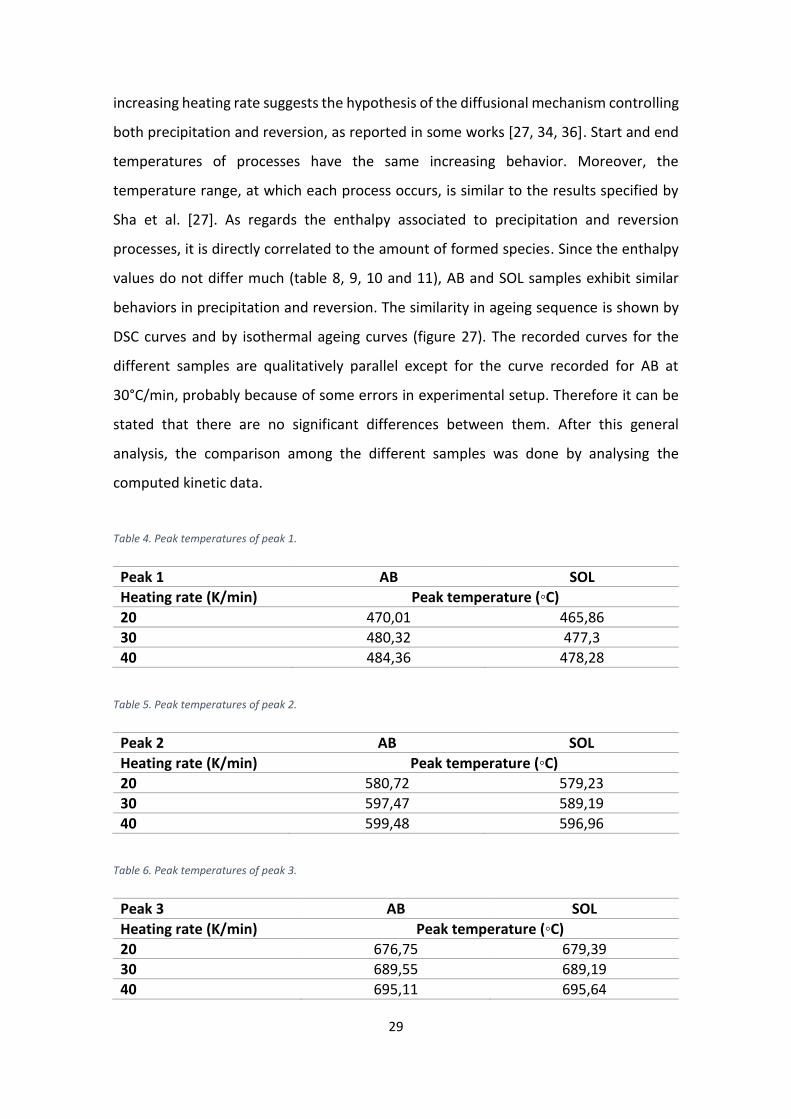
Table 4. Peak temperatures of peak 1. ....................................................................................... 29
Table 5. Peak temperatures of peak 2. ....................................................................................... 29
Table 6. Peak temperatures of peak 3. ....................................................................................... 29
Table 7. Peak temperatures of peak 4. ....................................................................................... 30
Table 8. Enthalpies of peak 1. ..................................................................................................... 30
Table 9. Enthalpies of peak 2. ..................................................................................................... 30
Table 10. Enthalpies of peak 3. ................................................................................................... 30
Table 11. Enthalpies of peak 4. ................................................................................................... 30
Table 12.Activation energies (kJ/mol) for all peaks in AB and SOL samples. .............................. 33
Table 13. Tensile tests results of AB and SOL samples, non-aged and peak aged at 460°C. ...... 37
Table 14. Peak hardness at different temperatures. .................................................................. 40
Table 15. Phases balance from chromatic analysis. .................................................................... 43
Table 16. Rietveld refinement results. ........................................................................................ 45
Table 17. Results of tensile tests on AB, peak aged and 540°C-8h samples. .............................. 47
Table 18. Diameter changes in as received and collected powders. .......................................... 57
Table 19.Hardness values of AB and SOL samples aged at 460°C. .............................................. 68
Table 20. Hardness values of AB and SOL samples aged at 490°C. ............................................. 69
Table 21. Hardness values of AB samples aged at 540°C and at 600°C. ..................................... 69

VII
ABSTRACT
18Ni-300 maraging steel parts were produced through selective laser melting (SLM)
technique, using manufacturer processing parameters. The samples were
microstructurally and mechanically characterized in the as build (AB) condition and after
a solution treatment (SOL). AB and SOL samples mechanical properties were compared
using ageing and tensile tests, while the ageing sequence was studied from a kinetic
point of view. The solution treatment resulted to have a detrimental effects on
mechanical performances because it changed the microstructure of AB samples. Ageing
behavior of AB samples was extensively studied, also considering the influence of
austenite volume fraction on mechanical properties. The austenite content seemed to
play a little role in modifying the material strength than other mechanisms. Tensile tests
showed that mechanical properties depends on layer orientation with respect to loading
direction and that porosity affects badly fracture elongation. Defects analysis allowed to
assess the influence of SLM system configuration on splats distribution and to identify
the mechanisms of porosity generation.
ESTRATTO
Campioni di acciaio maraging 18Ni-300 sono stati prodotti tramite la tecnica selective
laser melting (SLM). La microstruttura e le proprietà meccaniche dei campioni sono state
studiate nelle condizioni as build (AB) e dopo un trattamento di solubilizzazione (SOL). I
campioni sono stati confrontati in queste due condizioni tenendo conto delle curve di
invecchiamento isotermico e delle prove di trazione. La sequenza delle reazioni di
invecchiamento è stata analizzata con test cinetici. Non sono state rilevate differenze
nel comportamento di invecchiamento, anzi il trattamento di solubilizzazione ha causato
un abbassamento delle proprietà meccaniche. La ragione di questo fenomeno è la
diversa microstruttura dei campioni SOL rispetto a quelli AB. L’invecchiamento dei
campioni AB è stato ulteriormente indagato a differenti temperature al fine di
comprendere il grado di influenza dell’austenite residua sulle proprietà meccaniche. È
stato valutato l’effetto dell’austenite sull’allungamento a frattura e sullo sforzo di
snervamento. L’austenite ha un ruolo non significativo sull’allungamento e influenza

VIII
poco la resistenza del materiale. Le prove di trazione hanno mostrato che le proprietà
meccaniche dipendono anche dall’orientamento dei layer rispetto alla direzione di
carico. Questo comportamento e il basso allungamento a frattura di tutti i campioni
sono causati dalla porosità tipica di questa tecnica produttiva. Un’analisi della porosità,
delle polveri raccolte fuori dal substrato e delle superfici non modificate dei campioni
ha permesso di valutare l’influenza della configurazione del sistema SLM sulla
distribuzione degli splats e allo stesso tempo di identificare i meccanismi che originano
la porosità.
1
1 INTRODUCTION
1.1 SELECTIVE LASER MELTING
Additive manufacturing (AM) techniques, i.e. techniques that allow direct production by
means of material addition, have been developed in order to exploit advantages that
traditional processes based on material removal do not have. Additive processes usually
generate parts in a layered way. These techniques are well suited for rapid prototyping,
rapid manufacturing and rapid tooling, mainly for the production of small series of
components. All additive manufacturing techniques have in common some exclusive
advantages with respect to other processes. They allow the direct production of parts,
this means that components are generated at least in a near net shape quality. This
procedure allows AM to require less post-production processes. The major advantage is
the geometrical freedom, they have the capability to fabricate parts of very complex
shapes and geometries with the smallest feature size of about 100 µm [31]. This
geometrical flexibility and the direct production allow the production of customized
components. However some restrictions on geometry are given by the requirements of
unsolidified material removal from internal cavities and the need of supports to sustain
overhangs [13].
There are many different AM techniques; selective laser melting (SLM), electron beam
melting (EBM), direct metal deposition (DMD), inkjet printing are the most important.
Laser based techniques can process a high variety of materials such as polymers,
ceramics, composites, cermets metals and mixtures of them [1]. As regards metal
additive manufacturing, there can be different feed systems (powder-bed, powder feed
and wire feed systems) and different energy sources (laser, electron beam, arc) [44]. The
most used techniques to process metal are SLS and SLM. They are both powder-bed
systems and differ in the binding mechanism of the feed metal, i.e. sintering and melting
respectively. Selective laser melting process is an evolution of selecting laser sintering.
The difference is mainly in the energy provided to the metal powder, SLM is based on
the full melting of the handled material.

2
For metals, SLM process is considered the best between all AM techniques [13]. The
construction process is known as powder-bed process, because the fabrications
proceeds with selective melting of metallic or composite micrometric powders by a high-
power laser beam (100-400 W). With SLM, tridimensional parts are produced starting
from a CAD model, this model is divided in layers that are perpendicular to the growing
direction. So, parts are fabricated layer by layer.
The starting material in form of powder is deposited on a substrate plate, the deposited
layer is some tens of micrometre thick (30-50 µm). A laser beam selectively melts
powders under inert atmosphere according to the CAD model. Then the substrate
lowers down of a layer thickness and another layer of powder is deposited. The process
is repeated, the molten powder metallurgically binds with the preceding layer. The final
piece will be composed by the superposition of each layer.
SLM technique is very important because of the flexibility in practicable materials and
the capability to produce functional and structural components with properties
comparable to those of materials produced by conventional methods. A big advantage
with respect to SLS technique is the possibility to obtain fully dense parts without a post-
process densification [1].
Properties of SLMed components depend on accurate control of environmental
conditions and process parameters. The most important parameters are the laser power
and the beam scanning speed, they strongly influence density and superficial
morphology. Other parameters are layer thickness, scanning lines overlapping, scanning
Figure 1. Schematic description of a SLM printer [2].

3
strategy and powder properties (shape, size distribution, composition); all of them must
be optimized in order to obtain fully dense parts [2, 3]. The increase in scanning speed
and high layer thickness and the decrease of laser power are related to a reduction of
density, owing to a lower energy density input [10].
These process parameters modify the layer morphology which is very important
because linked to porosity creation. Defects can propagate because a layer with defects
does not allow a homogeneous deposition of the powder, moreover wrong parameters
lead to a lack of overlapping between scan tracks and therefore pores appear. Some
works show the relation between defects in a building layer and defects in preceding
layers [17]. In order to obtain a higher density and a better layer morphology, laser
remelting can be applied. If applied after scanning each layer, this remelting decreases
surface roughness and thus porosity. It is also used to process the surface layer to
enhance surface finishing. Also scanning strategies can be optimised to avoid these
phenomena; it is common to change scanning direction for each layer. Scanning strategy
is very important for the influence on residual stresses too. They arise from high thermal
gradients in the melt pool and high solidification velocity [6].
Regarding environmental conditions, the selective laser melting of metals must be
conducted in inert atmosphere to avoid surface oxidation. There would be a two-fold
problem: unwanted oxide inclusions can form between scan tracks and surface wetting
decreases giving the balling phenomenon. Balling is the effect given by the liquid metal
that does not wet oxidised surface and tends to form droplets, leaving a rough surface.
Roughness hinders a smooth layer deposition during the following layers and it lowers
density [5].
Many types of metals can be processed through SLM, both pure or as alloys. Titanium
and cobalt chromium alloys are used to produce customised biocompatible implants
and prosthesis. Most common metals for SLM production are aluminium alloys, nickel
alloys and different kind of steels such as stainless steels, tool steels, precipitation
hardening (PH) steels [2] [3] [14]. This thesis is focused on the study of a maraging steel.

4
1.2 MARAGING STEEL
Maraging steels are a group of martensitic steels with low-carbon and high-nickel
content. Their name comes from the contraction of “martensitic” and “aging”, because
these steels are subjected to aging heat treatments to highly improve hardness and
strength. Maraging steels are characterized by a high number of alloying elements,
mainly Ni, Co, Mo, Ti and Al, which are added to promote and produce intermetallic
precipitates. These steels exhibit excellent mechanical properties, combining high
strength with good toughness. Besides, they are suitable for SLM process because they
have a good weldability. Owing to the small size of the melt pool in the SLM process
(relative to the size of the substrate), cooling rates are typically very high. Their
properties make them well-matched for heavy duty applications in aerospace industry,
in engines or for the fabrication of dies and moulds for injection moulding, die casting,
extrusion and punching. This class of steels cannot be used for high temperature
applications. When temperature becomes higher than 500 °C there will be a strong
interference with the previous aging, leading to an excessive drop of strength [20].
The most common grades of maraging are 18% Ni ones, they are usually described with
a number (200, 250, 300, 350) that designates the approximate yield stress in ksi
(kilopound per square inch), so nominal yield stress for maraging goes from 1400 to 2400
MPa. Maraging steels with low nickel and cobalt content have been developed to
decrease costs, but their performances are lower than the results obtained with 18-Ni
grades.
High resistance is not obtained by solid solution and martensite strengthening because
of low carbon content; it is rather achieved through precipitation of intermetallic
compounds in the soft martensitic matrix. The common treatment steps are
solubilisation and aging. The material is solubilised in fully austenitic zone between
800°C and 900°C, then it is cooled down in order to achieve a supersaturated solid
solution. The resulting microstructure is lath martensite arranged in prior-austenite
grains [35]. After this heat treatment, some austenite may be retained due to nickel
presence, which is an austenite stabilizer [12]. A subsequent heat treatment (aging)
induces diffusive nucleation and growth of intermetallics based on Ni3Ti phase (or more

5
generally, Ni3X where X = Ti, Mo, V, W), followed by Fe2Mo or Fe7Mo6 precipitation [16,
19, 36]. In addition to precipitation, also the possibility to have austenite reversion must
be taken into account. Reversion, that is the martensite-to-austenite transformation,
occurs at temperature above 500 °C because of the dissolution of nickel-rich
precipitates. Then, the reverted austenite is retained in a room temperature leading to
mechanical properties change.
Ageing treatment can be conducted at different temperatures that range from 450 °C
up to 650 °C [7, 8, 22]. Strengthening is function of aging temperature and time, because
these two parameters influence precipitation kinetics. During ageing precipitation
strengthening and softening due to precipitates coarsening and to austenite reversion
occur. Owing to the high solid state diffusion enhanced by temperatures, the softening
and strengthening mechanisms may occur simultaneously. Therefore the strength peak
decreases as temperature increases because strengthening is readily overwhelmed by
softening. Since strengthening reaches a peak at different times for each temperature
and, as temperature increases, peaks occur before and have a lower value, a
compromise should be done by selecting temperature to have an appropriate strength
for a reasonable time.
Maraging steel strength relies on three contributions which are: strength of martensitic
matrix, solids solution strengthening and precipitation hardening. These contributions
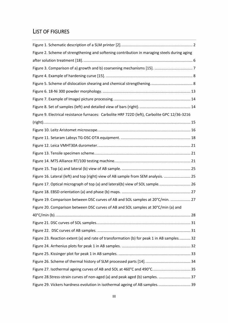
as function of ageing time are depicted in figure 2 [18]. Martensite strength is controlled
by the carbon content, by the decrease in grains dimensions and by dislocation density,
while solution strengthening depends on solute atom species and concentrations. Co
gives the higher contribution to solution strengthenig, followed by Ti and Mo. Ni and Al
have a lower effect that the other alloying elements [18]. As precipitation starts, solutes
depletion induces a drop in solid solution hardening. However, precipitation
strengthening gives the most important contribution to hardness.
6
1.2.1 Precipitation strengthening
In order to exhibit precipitation hardening, a material must undergo a solid-state phase
transformation induced by a change in alloying elements solubility due to a decrease in
temperature. In age hardenable alloys, precipitation can occur by homogeneous
nucleation, followed by particle growth and coarsening, and by spinodal decomposition
[16]. In case of maraging steels, only precipitation by nucleation happens. The
nucleation of second phases is a thermally activated process because supersaturated
solid solution decomposition requires atoms diffusion, and because provided thermal
energy helps to overcome the energy barrier to form a nucleus with a critical radius that
can grow further. The reason of that energy barrier is the Gibbs free energy for particles
nucleation. It is given by two terms, a positive one related to surface energy rise, when
radius and therefore interface area increases, and a negative one related to volume
increase. Before the critical radius all nuclei are metastable, they can grow or can
disappear. When the critical radius, corresponding to a critical Gibbs energy, is reached,
nuclei are stable and the growth is assured.
After nucleation, growth and coarsening of precipitates follow, both ruled by diffusion.
The main difference between growth and coarsening is the origin of diffusive atoms. For
growing particles, the diffusive atoms come from the surrounding saturated matrix; for
Figure 2. Scheme of strengthening and softening contribution in
maraging steels during aging after solution treatment [18].

7
coarsening particles, they come from matrix and from smaller dissolving particles.
Coarsening is due to chemical gradients and interfacial energy reduction (figure 3) [15].
Precipitation strengthening is achieved by producing a dispersion of obstacles to
dislocation motion. These obstacles increase the stress required to move dislocations,
making an alloy harder and stronger. Precipitates hinder dislocation movements
because of their interaction with dislocations. In general hardening depends on
structure, size which is the most influent parameter, and distribution of the second
phases. Also the volume fraction is important: if there are few particles, dislocation
pinning occurs in a smaller amount. At first a fine dispersion of numerous small coherent
precipitates forms. Increasing ageing time at elevated temperature, the dispersion
coarsens; the number of precipitates decreases and their size and spacing increases,
going from coherent to semi coherent precipitates. As ageing proceeds, coarsening and
spacing continue increasing, leading to incoherent and dispersed precipitates formation.
Dislocation hindering is less effective. After long ageing times, the equilibrium structure
is established and the coherency of second phases is completely lost [43].
Different strengthening mechanism are associated to precipitation hardening. Chemical,
coherency and dispersion strengthening are involved [16]. These mechanisms can be
operative simultaneously. Nevertheless, each mechanism tends to dominate the
dislocation-particle interactions at different ageing times. The typical strength-ageing
time curve (figure 4) shows two regions in which the different mechanisms act and a
peak strength that corresponds to a critical distribution of coherent or semi coherent
particles.
Figure 3. Comparison of a) growth and b) coarsening mechanisms [15].
8
In the first region, at early ageing times, the particles are small and coherent or semi
coherent. The dislocations are predisposed to cut through them in order to move and
the stress required moving those increases with precipitate radius. Here the dominant
mechanisms are coherency and chemical strengthening. Coherent precipitates show
crystal structure continuity with the matrix. If a misfit between reticular constants is
present, lattice strains arise at the interface. To move dislocations, they should be
subjected to an equal or higher stress than the one that particle exerts. Since particles
relax at interface when radius grows, this mechanism is important only in early stage of
ageing.
Chemical strengthening (figure 5) results from the energy consumed by dislocation
motion through the particles. The consumption comes from the energy requested to
create the additional matrix-precipitate interfaces, to form an antiphase boundary into
the precipitates [9] and to increase the dislocation line length.
In the second region precipitates become large and incoherent and it is difficult for a
dislocation to overcome the phase boundary between the host lattice and the
incoherent precipitation. This results in dislocation bowing around second phases. The
Figure 4. Example of hardening curve [15].
Figure 5. Scheme of dislocation shearing and chemical strengthening.

9
strengthening is due to increase of dislocation length because of bowing. Dislocation
lines close around particles forming loops; as deformation proceeds, more loops are
formed at each particle and bowing requires more energy, i.e. stress. Here hardness
decreases with time and the phenomenon is called overageing, indeed strengthening
effect of incoherent phases decreases with radius increase. In this case the increment of
yield strength follow the Orowan relationship [22]:
∆𝜎𝑂𝑅 = (0,538 𝐺𝑏√𝑓𝑣/𝑥) ∙ ln (𝑥/2𝑏)
where G is the shear modulus, b is Burgers vector, 𝑓𝑣 is volume fraction of precipitates
and x is diameter of precipitates. The strengthening mechanisms in maraging steels are
generally thought to be as said before [9]: in the early stages of aging, strengthening is
associated with the stress required for dislocations to cut through coherent precipitates.
As the precipitates coarsen and become semi-coherent, the stress required for
dislocations to cut the precipitates increases. Consequently, an increase in strength is
obtained. Further increase in particle size and spacing at long aging times leads to a
decrease in strength; the strength is governed by the Orowan equation.
The most important factors controlling strengthening behaviour in maraging steels are
nanometric precipitates formation and austenite reversion. These two central aspects
will be separately described in the following sections.
1.2.2 Precipitation in maraging steels
Maraging steel hardening is based on a nanometric intermetallic precipitates dispersion
due to ageing. Since precipitates are not stable phases, the time governs the
composition of all present phases and long ageing times would lead to an equilibrium
composition of austenite and ferrite [21]. At different temperatures, dissimilar second
phases are found, moreover the composition of precipitate phases depends on the alloy
composition. Nickel is the main alloying element because it is a basic constituent for
strengthening intermetallic compounds that it forms with Ti, Mo and Al. Addition of Co
reduces the solubility of Mo increasing the fraction of nickel intermetallics and
promoting the precipitation of Fe-Mo phase [18].

10
According to Ref. [8] and Ref. [11], phases in maraging steels are:
Table 1. Phases in maraging steels.
Phase Composition Crystal structure
Martensite (α-Fe) BCC
Austenite (γ-Fe) FCC
ω A2B Hexagonal
S A8B Hexagonal
X A3B Hexagonal
µ Fe7Mo6 Rhombohedral
Η Ni3(Ti,Mo) Hexagonal
Laves phase Fe2Mo Hexagonal
Ni3Mo Ni3Mo Orthorhombic
For ageing at low temperatures, from 400°C to 450°C, ordered and coherent phases such
as ω, S, X and µ in the martensitic matrix appear [7, 19, 22]. These precipitates are not
investigated because they have not a high influence on strength at common ageing
temperatures.
For aging at temperatures higher than 450°C, rapid hardening occurs. Nor the order of
precipitation, neither which precipitates are responsible for strengthening, are fully
understood and the composition Mo-rich phase appearing in late stages of ageing is still
discussed. A reason of this uncertainties is that precipitates are nanometric, thus
problematic to be characterized. However, hardening is attributed to precipitation of
Ni3(Ti,Mo) and Fe-Mo phase preferentially in dislocations in the martensitic matrix and
at lath boundaries [7, 19, 35].
The first precipitate is Ni3Ti and it is believed to provide the higher contribution to
strength. Fe and Co can substitute Ni in a small amount, while Ti atoms can be
substituted by Mo and Al so this phase is usually identified as Ni3(Ti,Mo). These
precipitates can be rod-shaped, or ellipsoidal [11, 18] with approximate width and
length of 5 nm and 10-20 nm respectively [22] and can effectively resist to coarsening.

11
Along with the η phase, also Ni3Mo precipitates in form of needle-like clusters [11]. It is
a metastable phase that dissolves as ageing proceeds.
These two phases appear at early stage of aging because Fe-Mo precipitates are not
coherent with the matrix. Then the tendency to reach system equilibrium promotes
Ni3Mo dissolution. Through this the matrix enriches in Mo, producing spherical Mo-rich
phase. The phase composition has not been clearly identified; in some works it is
recognized as a Laves phase (Fe2Mo) [8, 22], in other works as a µ phase (Fe7Mo6) [11,
23]. Whatever it is, it has a lower effect on strength respect to η and Ni3Mo and it
appears especially in the overaged conditions.
Ageing at temperatures between 500°C and As induces a very fast precipitation for which
overageing is rapidly reached. In this temperature range another reaction accompanies
the precipitation and follows the dissolution of Ni3Mo, it is the austenite reversion.
Summarizing, the peak aged condition of maraging steels is reached when a critical
dispersion of nanometric features appears; it is mainly composed of Ni3(Ti,Mo) and
Ni3Mo particles with a low fraction of Fe-Mo phase.
1.2.3 Austenite reversion
Loss of strength in maraging steels is associated more decisively with reversion of
martensite to austenite rather than coarsening of precipitates [9, 26]. The reason of this
behavior is that reversion of austenite, beyond the softness of γ-Fe respect to
martensite, is linked to dissolution of precipitates.
Austenite reversion occurs essentially in every maraging steel, but the extent of this
transformation relies on temperature. At temperatures higher than 500°C, the
formation of reverted austenite which has been retained at room temperature, occurs
together with hardening, hampering the achievement of high strength. Austenite
formation occurs at the same time of Fe2Mo as consequence of the dissolution of Ni3Mo
precipitates. The decomposition enriches the martensitic matrix in Mo and Ni, the last
being an austenite stabilizer [7, 19]. Thus, high ageing temperatures promote austenite
by a diffusion controlled reaction:
𝛼′ → 𝛼 + 𝛾

12
where 𝛼′ is the martensitic matrix, 𝛼 is a low Ni BCC phase and 𝛾 is the Ni-enriched
austenite.
The sequence of austenite formation as function of temperature and time has been
extensively investigated. About time dependence, γ-Fe fraction is negligible in
solubilized and not aged parts. As ageing begins, austenite appears mainly at the lath
martensite boundaries but also at prior austenite grain boundaries; moreover, it can
grow around retained austenite regions [23]. After that austenite pockets grow along
boundaries and nucleate within the martensite lath [21, 22, 24]. At long ageing times
the volume fraction reaches an almost constant value [21, 25, 26].
The content of retained austenite also depends on temperature, it increases with the
ageing temperature until a peak value and then decreases. This phenomenon relies on
the composition of austenite and thus on the martensite start temperature Ms. Since Ms
decreases with the increasing content of nickel in austenite and since ageing
temperature reduces this content [24, 25], at higher temperatures correspond lower
fractions of reverted austenite. This is likely to occurs at temperatures about 600°C.
Austenite is related to softening of the material, its presence modifies mechanical
properties. It can have detrimental or beneficial effects depending on its volume
fraction. The retention of small quantities at lath grain boundaries in slightly overaged
samples is found to increase toughness and ductility with a little drop of yield strength
[12]. The material can exhibit a good combination of strength and toughness and the
mechanism involved in toughness increase is the increment in crack path length due to
the presence of small austenite packets at lath boundaries as shown by Yang et al. [22].
However, for prolonged ageing austenite retention affects badly all mechanical
properties. Yield strength and toughness decrease; brittleness is related to the presence
of overaged particle which act as nucleation points for cracks, yield drop to the extensive
presence of γ-Fe at grain boundaries [21].
Considering the afore-mentioned phenomena, the achievement of desired mechanical
properties in maraging steel relies on a careful optimization of ageing times and
temperatures.

13
2 MATERIALS AND METHODS
2.1 MATERIAL
The material used for the experiments is a 18-Ni 300 maraging steel (1.2709) in form of
gas-atomized powder. Chemical composition of the alloy is given in table 2. Figure 6
shows the typical morphology of powders. Most of powder particles are spherical or
quasi-spherical, this shape allows particle to flow without impediments during
deposition. Thus a homogeneous layer with less defects is obtained [10]. Particle size
distribution, measured by image analysis, shows a mean dimension of 24 µm and a
maximum dimension of 60 µm. An example of image analysis is shown in figure 7. There
a comparison between the as received powder and a batch of powder collected around
the base plate is also proposed. This topic will be discussed in a following section.
Table 2. Chemical compositon (wt%) of studied steel.
Ni Mo Co Ti Al Si Fe
17,6 5,3 9,6 0,7 0,009 0,2 Balance
Figure 6. 18-Ni 300 powder morphology.

14
2.2 PROCESSING METHODS
2.2.1 Selective laser melting
The samples have been produced by SLM process, using a Renishaw AM250 SLM system.
The set of samples is composed of square section prisms of dimensions 10 mm × 10 mm
× 70 mm, horizontally and vertically oriented as shown in figure 8. The terms horizontal
and vertical refer to the direction of the longitudinal axis with respect to the base plate.
Bars are printed under argon atmosphere by a single mode fiber laser with a power of
200 W and an estimated beam diameter at a focal point of 75 µm. Scan lines are
composed by discrete and partially overlapped melted points. The spots are exposed to
the radiation for a fixed time (t) and their distance is called point distance (dP). The laser
moves from the end of each scan line to an adjacent one and overlaps it partially. The
distance between adjacent scan lines is defined as the hatch distance (dH). The
Figure 7. Example of ImageJ picture processing.
Figure 8. Set of samples (left) and detailed view of bars (right).
15
parameters dH, dP, and t were set to 80 µm, 65 µm, and 80 µs, respectively according to
their optimization and manufacturer data. The thickness of each powder layer was set
to 40 µm. A meander scanning strategy and the scanning direction rotation of 67° after
each layer is used to produce samples.
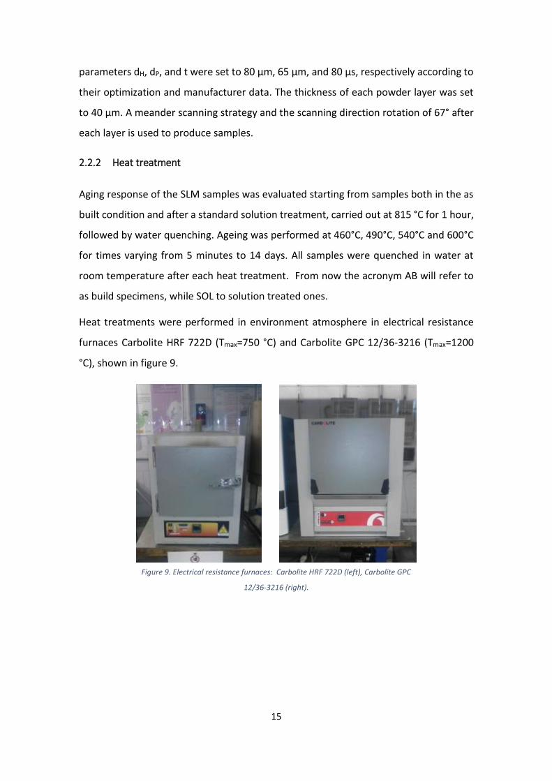
2.2.2 Heat treatment
Aging response of the SLM samples was evaluated starting from samples both in the as
built condition and after a standard solution treatment, carried out at 815 °C for 1 hour,
followed by water quenching. Ageing was performed at 460°C, 490°C, 540°C and 600°C
for times varying from 5 minutes to 14 days. All samples were quenched in water at
room temperature after each heat treatment. From now the acronym AB will refer to
as build specimens, while SOL to solution treated ones.
Heat treatments were performed in environment atmosphere in electrical resistance
furnaces Carbolite HRF 722D (Tmax=750 °C) and Carbolite GPC 12/36-3216 (Tmax=1200
°C), shown in figure 9.
Figure 9. Electrical resistance furnaces: Carbolite HRF 722D (left), Carbolite GPC
12/36-3216 (right).

16
2.3 CHARACTERIZATION METHODS
2.3.1 Optical microscopy
Optical microscopy analyses were performed to examine the microstructure of as built,
solution treated and aged samples. A Leitz Aristomet microscope (figure 10) was used
at different magnifications from 25x to a maximum of 500x. Samples preparation
required grinding and polishing down to 1 µm grit size and etching. Modified Fry’s
reagent (1 g CuCl2, 50 mL HCl, 150 mL H2O, 50 mL HNO3) was used on AB and SOL
specimens, while Picral etch (4% picric acid in ethanol) was used on aged samples to
distinguish between austenite and martensite constituents.
2.3.2 Scanning electron microscopy
Microstructural observations, powder morphology evaluation, fractography analyses
and the analysis of top surfaces of as build samples were carried out by Zeiss EVO 50
scanning electron microscope (SEM). This instrument can detect secondary and
backscattered electrons, moreover it can perform electron back‐scattered diffraction
(EBSD) and dispersive x-ray spectroscopy (EDX). This permits to detect texture and to
assess phases composition.
SEM scans the investigated material by means of a high energy collimated electron
beam. Having electrons a lower wavelength than light, SEM allows to obtain higher
Figure 10. Leitz Aristomet microscope.

17
resolution and higher depth of focus. The material responses to the electron beam are
backscattered electrons, secondary electrons and x-rays emissions. Backscattered
electrons consist in the beam electrons that are subjected to elastic scattering and are
reflected out of the specimen. They can be used to discriminate between areas with
different chemical composition. On the base that heavy elements backscatter electrons
better than light elements, brighter zones will correspond to heavier elements. Another
advantage of backscattered electrons is the capability to be diffracted according to
Bragg’s law. The EBSD technique uses diffracted backscattered electrons to characterize
the crystalline lattice geometry of the material. Structure, crystal orientation and phase
of materials can be detected by using crystallographic data only.
Secondary electrons are emitted from the valence band of atoms excited by the
electron beam. Since they are generated by inelastic collisions, which occurs in few
nanometers of depth, this response is the best to study material morphology.
The X-ray emission is exploited in electron dispersive x-ray spectroscopy (EDX). It is an
analytical technique that allows to obtain elemental characterization of the material. It
relies on the fact that each element has a unique emission spectrum. Measuring the
spectrum peak intensities after an appropriate calibration, a quantitative evaluation of
the chemical composition can be attained.
Samples were prepared in the same way as for optical analysis, i.e. grinding, polishing
and etching. In case of EBSD analysis, the preparation consisted in grinding and polishing
down to 1 µm grit size followed by a prolonged polishing with colloidal silica. This
polishing was necessary to reach the very low roughness surface required by EBSD.
2.3.3 Stereoscope
The analysis of the as build top surfaces was performed with a Zeiss Axiocam ERc 5s
stereoscope. Images were taken at 20x magnification to investigate the presence of
splats and particles. The ImageJ software was used to process pictures and collect
quantitative information by image analysis technique.

18
2.3.4 Differential scanning calorimetry
Differential scanning calorimetry analyses were performed using a Setaram Labsys TG-
DSC-DTA equipment (figure 11) in argon inert atmosphere at three different heating
rates (20, 30, 40°C/min) between 20°C and 1540°C. AB and SOL specimens were
prepared by cutting small samples having a weight of about 100 mg.
The aim of DSC tests is to assess reactions and phase changes sequence. The DSC testing
instrument consists in an empty reference crucible, and another one containing the
studied sample. They are simultaneously heated and kept at the same temperature. The
amount of energy provided to the sample during endothermic processes or removed
during exothermic ones, is recorded as a function of furnace temperature. A DSC curve
shows the heat flow, that is the amount of energy exchanged by the sample, versus
temperature. If the heat flow direction is outward the sample, it is considered as
positive. Using this convention, the curve will show maxima for exothermic processes
and minima for endothermic processes.
As DSC makes possible to follow phase transformation sequence under precise non-
isothermal heating, it has been used to describe solid state transformation kinetics.
Kinetic parameters for each process, such as activation energy, can be evaluated
studying the peaks of DSC curves through different models. In order to simplify the
problem, all these models describe the transformation rate as the product of two
independent functions, one depending on the reaction extent, the other one depending
on the temperature:
Figure 11. Setaram Labsys TG-DSC-DTA equipment.

19
𝑑𝑌/𝑑𝑡 = 𝑓(𝑌)𝑘(𝑇) (1)
where 𝑌 is the degree of transformation, 𝑓(𝑌) is the reaction model and 𝑘(𝑇) is the
reaction constant. The reaction constant is described by an Arrhenius-type function [27]:
𝑘(𝑇) = 𝑘0exp (− 𝐸𝑎 𝑅𝑇⁄ ) (2)
where 𝐸𝑎 is the activation energy of the process, 𝑘0 is a constant and 𝑅 is the gas
constant. The reaction extent of the transformation at any given time is taken equal to
the fraction of heath released or absorbed [27], so:
𝑌(𝑡) =∫ 𝐻 𝑑𝑡
𝑡
𝑡𝑆
∫ 𝐻 𝑑𝑡𝑡𝐸
𝑡𝑆
where 𝐻 is the heat flow, 𝑌(𝑡) is the reaction extent at any given time t, 𝑡𝑆 and 𝑡𝐸 are
the start and end times of the considered transformation. The equation denominator is
the total enthalpy for the transformation corresponding to a selected peak.
Isoconversional methods are used to determine the activation energy from constant
heating rate experiments. These methods rely on the measurement of temperatures at
which the same process, at different heating rates, reach the same transformation
degree. Methods can be classified in two groups, namely type A and type B [28].
Type A methods, also known as Friedman’s or rate-isoconversion methods, do not use
any mathematical approximation. They determine the transformation rate at a fixed
extent of reaction for various heating rates. Possible errors come from the inaccuracy of
the baseline and the determination of the temperature at constant transformation
degree.
This method is obtained by inserting equation (1) in equation (2):
𝑑𝑌
𝑑𝑡= 𝑓(𝑌)𝑘0exp (−
𝐸𝑎
𝑅𝑇)
Taking the logarithm and considering a fixed transformed fraction 𝑌𝑖 at temperature 𝑇𝑗:
ln [(𝑑𝑌
𝑑𝑡)
𝑌𝑖
] = ln[𝑓(𝑌𝑖)𝑘0] − (𝐸𝑎
𝑅)
1
𝑇𝑗

20
A straight line is obtained by linear regression of the plot ln [(𝑑𝑌
𝑑𝑡)
𝑌𝑖
] versus 1
𝑇𝑗 for each
heating rate, and its slope is − (𝐸𝑎
𝑅). In this way the activation energy is obtained.
Type B methods, which includes also Kissinger’s method, use approximations and are
based on the temperature integral [28]. The method is derived starting from equation
(1) and (2); the final result is:
ln (𝑇𝑝
2
Φ) = −
𝐸𝑎
𝑅𝑇𝑝+ 𝐶
where 𝑇𝑝 is the peak temperature of the studied transformation and Φ the heating rate.
By plotting ln (𝑇𝑝
2
Φ) versus 1 𝑇𝑝⁄ the activation energy can be evaluated.
2.3.5 Vickers micro-hardness
In order to follow strength evolution during aging, hardness as a function of time at
constant temperature was measured. Isothermal aging curves were acquired using
Vicker’s micro-hardness test. This test is performed by applying a constant load on a
pyramid-shaped diamond indenter with square base and angle between opposite faces
of 136°. The indenter penetrates the material leaving a depression in the material. The
hardness number is determined by the load over the surface area of the indentation and
can be expressed in kilograms-force per square millimeter or in Pascal. The hardness of
the material calculated in kgf/mm2 is proportional to the applied load 𝐹 and to the
diagonals mean length 𝑑 according to 𝐻𝑉 = 1,8544𝐹
𝑑2.
Before testing, all the samples were polished by abrasive papers with grit sizes from 320
up to 2500 to avoid measurement errors. Tests were performed with a Leica VMHT30A
durometer (figure 12), using a load of 2 kg for 15 seconds.

21
2.3.6 Tensile testing
Tensile tests were performed on cylindrical samples machined out from the SLM
processed bars, with dimensions d=4 mm, Lc= 14 mm, LTOT=70 mm, R=3 mm and S0=
12,57 mm2, as depicted in figure 13. A first series of tests was performed on vertically
and horizontally oriented specimens to evaluate the effect of layer orientation on
mechanical properties. Printed bars were machined in order to obtain tensile specimens
that were subjected to different heat treatments before testing. Three specimens per
condition were tested. Tests were carried out at room temperature with a crosshead
speed of 1 mm/min, using a MTS Alliance RT/100 testing machine (figure 14).
Figure 12. Leica VMHT30A durometer.
Figure 14. MTS Alliance RT/100 testing machine.
Figure 13. Tensile specimen scheme.

22
2.3.7 XRD analysis
A PANanalitica X-Pert PRO diffractometer, equipped with a TMS X’Celerator sensor, was
used to collect diffraction patterns. A X ray radiation peak Cu Kα with wavelength 1,5418
Å was used. Patterns were collected from 30° to 83° with a step size of 0,02°.
Pattern peaks were identified using literature references and Maud software. Rietveld
refinement method, performed with Maud, allowed to make a quantitative phase
analysis. Table 3 gives the structural parameters used for the refinement.
Table 3. Structural parameters of maraging phases.
Symmetry Spatial group Lattice constants
Martensite Tetragonal I4/mmm a=2.8747 Å c=2.8866 Å
Austenite Cubic Fm-3m a = 3.6136 Å
Number and position of peaks in XRD patterns follow the Bragg’s diffraction law
2𝑑 sin 𝜃 = 𝑛𝜆 . The peaks are a function of the angular position and of the crystal
structure variables. Height and width of each peak are given by a combination of
incident intensity, sample characteristics and instrumental deviations such as beam
divergence, non-monochromatic radiation and alignment issues. If there is more than
one phase in the sample, the intensity of the peaks corresponding to one phase is
proportional to its volume fraction. This phenomenon is that on which is based the
quantitative phase analysis. Rietveld refinement consists in the generation of a fitting of
a generic experimental pattern; it uses a least square method to match a theoretical
pattern with the real one. The theoretical computed intensity of i-th reflection of phase
k will be [30]:
𝐼𝑖𝑘 ∝ 𝐼
𝑓𝑘
𝑉𝑘2 ∙ 𝐶𝑖,𝑘
where 𝐼 is the incident intensity, 𝑓𝑘 is the k-th phase volume fraction, 𝑉𝑘 is the k-th
phase cell volume and 𝐶𝑖,𝑘 contains absorption, structure, texture, Lorentz polarization
factors and profile peak shape function. The total intensity of calculated i-th
reflection 𝐼𝑖𝑐𝑎𝑙𝑐 will be the sum of all 𝐼𝑖
𝑘 and the background factor 𝑏𝑘𝑔𝑖. The refinement
purpose is to minimize the residual function WSS:

23
𝑊𝑆𝑆 = ∑ 𝑤𝑖(𝐼𝑖𝑒𝑥𝑝 − 𝐼𝑖
𝑐𝑎𝑙𝑐)2
𝑖
where 𝑤𝑖 = 1 𝐼𝑖𝑒𝑥𝑝⁄ is the statistical weight, 𝐼𝑖
𝑒𝑥𝑝 is the experimental reflection
intensity, 𝐼𝑖𝑐𝑜𝑚𝑝 is the computed fitting intensity. The reliability of the fit is recognized
by comparing two factors, 𝑅𝑤𝑝 (weighted profile R-factor) and 𝑅𝑒𝑥𝑝 (expected R-factor),
the goodness of the fitting 𝐺𝑜𝑓𝐹 = 𝑅𝑤𝑝 𝑅𝑒𝑥𝑝⁄ [29]. Having N data points and P
parameters, R-factors are:
𝑅𝑤𝑝 = [∑ 𝑤𝑖(𝐼𝑖𝑒𝑥𝑝 − 𝐼𝑖
𝑐𝑎𝑙𝑐)2
𝑖
∑ 𝑤𝑖(𝐼𝑖𝑒𝑥𝑝)2
𝑖
⁄ ]1/2
𝑅𝑒𝑥𝑝 = [(𝑁 − 𝑃) ∑ 𝑤𝑖(𝐼𝑖𝑒𝑥𝑝)2
𝑖
⁄ ]1/2

24
3 RESULTS AND DISCUSSION
3.1 AS BUILD AND SOLUTION TREATED SAMPLES COMPARISON
First, an investigation between solution treated and as build samples was conducted.
The aim was to assess the microstructural differences and the changes in the achievable
strength between AB and SOL samples. In order to analyse microstructures optical
microscopy, SEM and EBDS examinations were carried out. Regarding the strength,
ageing treatments, hardness tests and tensile tests were performed. Kinetic analysis was
done to evaluate the ageing sequence and the activation energies.
3.1.1 Microstructural characterization
Optical and SEM micrographs were taken to assess macro and microstructure of as build
and heat treated bars. Bars were sectioned and top (perpendicular to building direction)
and lateral (parallel to building direction) surfaces were inspected. Analyses were
performed on samples AB and SOL without ageing.
As build microstructure
As regards AB sample, the images taken with the optical microscope show how the SLM
process occurs, that is the interconnection among molten lines. In the top view (figure
15a) we can see that scanning direction of different layers is rotated, moreover also
some distinct pools of the same track resulting from the pulsed laser beam are visible.
The lateral view (figure 15b) clearly shows the overlapping among different scan lines in
order to avoid porosity. This is the typical appearance of as build printed metals as
shown for instance in [10], [23], [32] and [33].
In SEM micrographs the solidification structure is clearly recognised as composed by
very fine elongated grains that result from cellular solidification. The intercellular
spacing is in the sub-micrometer scale (≤1 µm). In figure 16 the top view suggests the
presence of epitaxial growth between scan track boundaries. These are common
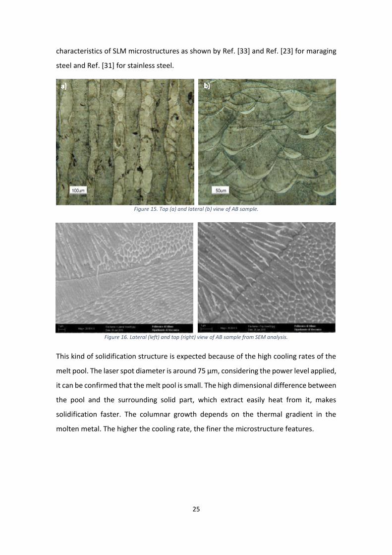
25
characteristics of SLM microstructures as shown by Ref. [33] and Ref. [23] for maraging
steel and Ref. [31] for stainless steel.
This kind of solidification structure is expected because of the high cooling rates of the
melt pool. The laser spot diameter is around 75 µm, considering the power level applied,
it can be confirmed that the melt pool is small. The high dimensional difference between
the pool and the surrounding solid part, which extract easily heat from it, makes
solidification faster. The columnar growth depends on the thermal gradient in the
molten metal. The higher the cooling rate, the finer the microstructure features.
Figure 15. Top (a) and lateral (b) view of AB sample.
Figure 16. Lateral (left) and top (right) view of AB sample from SEM analysis.

26
Solution treated microstructure
The microstructure of SOL sample is completely different because of the high
temperature treatment and the following rapid quench. In the optical micrograph
(figure 17), it is visible that the previous cellular microstructure completely disappears
and scan line boundaries are no more visible. The cellular solidification structure is
replaced by the characteristic martensitic matrix composed by packets of martensite
blocks. These blocks consist in fine parallel laths as shown in literature [35]. By
comparing this microstructure with the AB one, we can see that it is coarser with bigger
features and a different structure.
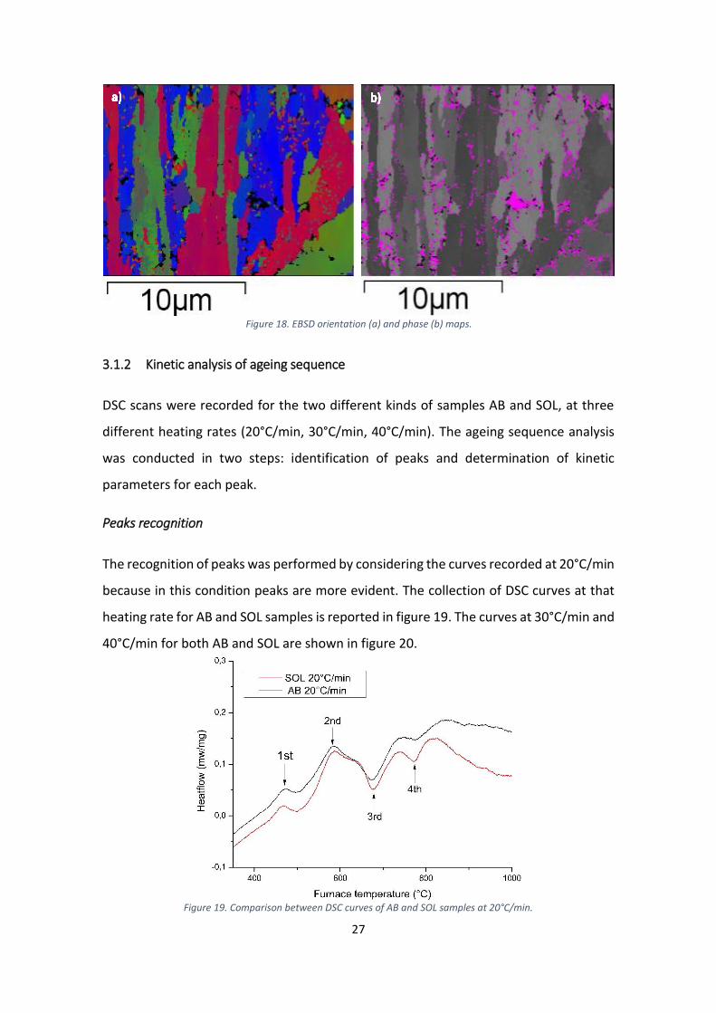
EBSD was carried in order to evaluate the grain orientation and to phase map. The
coarse martensitic structure is evident in the EBSD orientation image (figure 18a) that
shows the martensite blocks. As we can see in figure 18b, fractions of retained austenite
(pink) were likely to be found at martensite (grey scale) boundaries. This result agrees
with literature results that indicate martensite lath boundaries the place where γ-Fe
retains and stars to nucleate when reversion occurs [21, 24, 35]. The presence of
austenite in the solution treated sample also suggests the possibility to find it in the AB
specimens. No precipitates were detected because of their small sizes.
Figure 17. Optical micrograph of top (a) and lateral(b) view of SOL sample.
27
3.1.2 Kinetic analysis of ageing sequence
DSC scans were recorded for the two different kinds of samples AB and SOL, at three
different heating rates (20°C/min, 30°C/min, 40°C/min). The ageing sequence analysis
was conducted in two steps: identification of peaks and determination of kinetic
parameters for each peak.
Peaks recognition
The recognition of peaks was performed by considering the curves recorded at 20°C/min
because in this condition peaks are more evident. The collection of DSC curves at that
heating rate for AB and SOL samples is reported in figure 19. The curves at 30°C/min and
40°C/min for both AB and SOL are shown in figure 20.
Figure 18. EBSD orientation (a) and phase (b) maps.
Figure 19. Comparison between DSC curves of AB and SOL samples at 20°C/min.

28
The attribution of each peak was done by comparing the obtained results with data
found in literature for the same alloy. There are four peaks: the first (1) and the second
(2) are exothermic and linked to precipitation, while the third (3) and the fourth (4) are
endothermic and linked to austenite reversion and precipitate dissolution. According to
literature, peak 1 is associated to the first precipitation stage, that is carbide and
coherent phases precipitation, and to martensite recovery [27]. Peak 2 corresponds to
the formation of the main strengthening precipitates, Ni2(Ti, Mo) and Fe7Mo6 or Fe2Mo
[27, 34]. The first endothermic peak, peak 3, is connected to the austenite reversion by
diffusion, while the second one, peak 4, to the 𝛼′ → 𝛾 transformation by shear and to
dissolution of precipitates [27, 34, 36].
About the presence of two different peaks corresponding to the austenite reversion,
Kapoor and Batra [36] report that the splitting in two step of 𝛼′ → 𝛾 transformation in
dilatometric curves is enhanced by slow heating rates. They report the onset of the
splitting at heating rates slower than 120°C/min in a 350 maraging steel. The obtained
DSC curves seem to have a good agreement with this report; as we can see in figure 19
and 20 the difference between peak 3 and peak 4 tends to become less pronounced as
heating rate increases. At lower heating rates, martensite starts to transform into
austenite by a long-range diffusion process; at sufficiently high temperatures (>720°C)
the remaining austenite transforms into austenite by a shear mechanism [27, 36]. The
reason of this behaviour is that diffusion has no time to take place at fast heating rates.
The peak temperatures for all peaks and conditions are listed in table 4, 5, 6 and 7. Even
if the exact values of peak temperatures are not very significant, their increase with
a) b)
Figure 20. Comparison between DSC curves of AB and SOL samples at 30°C/min (a) and 40°C/min (b).
29
increasing heating rate suggests the hypothesis of the diffusional mechanism controlling
both precipitation and reversion, as reported in some works [27, 34, 36]. Start and end
temperatures of processes have the same increasing behavior. Moreover, the
temperature range, at which each process occurs, is similar to the results specified by
Sha et al. [27]. As regards the enthalpy associated to precipitation and reversion
processes, it is directly correlated to the amount of formed species. Since the enthalpy
values do not differ much (table 8, 9, 10 and 11), AB and SOL samples exhibit similar
behaviors in precipitation and reversion. The similarity in ageing sequence is shown by
DSC curves and by isothermal ageing curves (figure 27). The recorded curves for the
different samples are qualitatively parallel except for the curve recorded for AB at
30°C/min, probably because of some errors in experimental setup. Therefore it can be
stated that there are no significant differences between them. After this general
analysis, the comparison among the different samples was done by analysing the
computed kinetic data.
Table 4. Peak temperatures of peak 1.
Peak 1 AB SOL
Heating rate (K/min) Peak temperature (◦C)
20 470,01 465,86
30 480,32 477,3
40 484,36 478,28
Table 5. Peak temperatures of peak 2.
Peak 2 AB SOL
Heating rate (K/min) Peak temperature (◦C)
20 580,72 579,23
30 597,47 589,19
40 599,48 596,96
Table 6. Peak temperatures of peak 3.
Peak 3 AB SOL
Heating rate (K/min) Peak temperature (◦C)
20 676,75 679,39
30 689,55 689,19
40 695,11 695,64

30
Table 7. Peak temperatures of peak 4.
Peak 4 AB SOL
Heating rate (K/min) Peak temperature (◦C)
20 776,05 771,89
30 779,47 775,26
40 780 777,06
Table 8. Enthalpies of peak 1.
Peak 1 AB SOL
Heating rate (K/min) Enthalpy (J/g)
20 2,08 2,03
30 1,47 3,8
40 1,53 2,18
Table 9. Enthalpies of peak 2.
Peak 2 AB SOL
Heating rate (K/min) Enthalpy (J/g)
20 8,74 8,79
30 9,57 7,89
40 10,52 7,01
Table 10. Enthalpies of peak 3.
Peak 3 AB SOL
Heating rate (K/min) Enthalpy (J/g)
20 -10,28 -8,78
30 -13,19 -10,47
40 -13,99 -7,23
Table 11. Enthalpies of peak 4.
Peak 4 AB SOL
Heating rate (K/min) Enthalpy (J/g)
20 -2,41 -3,1
30 -1,56 -4,16
40 -1,9 -2,73

31
Determination of activation energy
DSC scans were performed at three different heating rates for each sample in order to
extract kinetic data. The obtained curves for AB and SOL samples are reported in figures
21 and 22.
The reaction extent 𝑌 of precipitation and the rate of precipitation 𝑑𝑌 𝑑𝑇⁄ were
computed for each sample, examining all peaks. An example of the results of the analysis
of peak 1 in AB sample is depicted in figure 23. The other curves and plots are reported
in appendix 5.4-5.7. The transformation degree curves always show a characteristic
sigmoid shape and they shift at higher temperatures as heating rate increases. Also
𝑑𝑌 𝑑𝑇⁄ plots show the same behavior; these features confirm that precipitation and
reversion are controlled by diffusion.
Figure 21. DSC curves of SOL samples.
Figure 22. DSC curves of AB samples.

32
By working out the data recorded with DSC tests the activation energies were evaluated.
The Friedman method allows to obtain the so-called Arrhenius plots, i.e. 𝑑𝑌𝑑𝑡⁄ vs 1 𝑇⁄ . The
activation energy was computed through the average slope of the calculated linear fittings.
The application of this method on peak 1 of AB samples is shown in figure 24.
Figure 24. Arrhenius plots for peak 1 in AB samples.
Figure 23. Reaction extent (a) and rate of transformation (b) for peak 1 in AB samples.
a) b)

33
Also the Kissinger method was applied and the plots ln (𝑇𝑝
2
Φ⁄ ) vs. 1 𝑇⁄ were obtained. The
calculated slope is proportional to the activation energy. The method applied again on peak 1 of
AB samples is reported in figure 25. The resulting activation energies for each peak and sample
are listed table 12.
Table 12.Activation energies (kJ/mol) for all peaks in AB and SOL samples.
Ea (kJ/mol) Peak 1 Peak 2 Peak 3 Peak 4
AB SOL AB SOL AB SOL AB SOL
Kissinger 204,97 205,73 174,48 274,41 264,21 310,27 1406,75 1189,49
Friedman 196,51 179,68 183,61 315,68 358,75 625,09 1491,88 1167,43
First of all, only the result obtained with Kissinger method are considered reliable
because they are coherent with literature reports. The high differences between the
results achieved by applying Kissinger and Friedman for peaks 2 and 3 should be
attributed to the difficulties in evaluating the start and end temperatures. No results
were found in literature for the activation energies of peak 1 and peak 4, but a
qualitative consideration can be made about peak 1. Since peak 1 is related to short-
range diffusion such as clustering, there are no differences in activation energy between
AB and SOL specimens. On the contrary the processes related to long-range diffusion,
i.e. main strengthening precipitates formation (peak 2) and austenite reversion by
diffusion (peak 3), show differences in activation energy.
Figure 25. Kissinger plot for peak 1 in AB samples.

34
As regards precipitation Sha et al. [27] reported an activation energy of 205,1 kJ/mol in
the case of wrought 250 maraging steel. Kapoor and Batra [36] found a value of 265
kJ/mol in 350 maraging steel. Menapace et al. [34] obtained the values of 150 kJ/mol
and 269 kJ/mol corresponding to a 300 maraging steels sintered in two different
conditions; the dissimilar energy values are attributed to the difference in grain sizes
and defects number. Looking at the Kissinger method results for peak 2, we can see that
the energies given by Ref. [34] and Ref. [36] are close to the SOL precipitation energy,
while the smaller value in [34] is closer the AB activation energy.
For austenite reversion activation energies of 342 kJ/mol [27] and of 423 kJ/mol [36]
were reported. The corresponding result for SOL is similar to the first value. It is notable
that SOL activation energies are comparable to those for lattice diffusion of Ni (245
kJ/mol), Ti (272 kJ/mol), Mo (238 kJ/mol) in α-Fe. This confirms that both reversion and
precipitation are processes under diffusive control. The activation energy of AB samples
is lower than SOL samples owing to the different microstructures. The fine cellular AB
microstructure facilitates diffusion: the smaller the crystalline size is, the smaller the
activation energy is because of the effects of grain boundaries on diffusion.
3.1.3 Ageing tests
Since maraging is a precipitation hardenable alloy, it can be subjected to hardening
during the printing process. During processing the steel is exposed to a complex thermal
history depicted in figure 26.
The powder production and the laser melting involve high cooling rates so that
precipitation cannot occur. However the heat provided to melt powders may modify the
Figure 26. Scheme of thermal history of SLM processed parts [14].

35
hardness in region near the melt pool, i.e. in the heat affected zone. So the chance to
have precipitation hardening is localized in the already solidified material. The heat
affected zone does not reach the melting temperature but it is subjected to a cyclic
heating in the right temperature range to have ageing. This can be considered as an
intrinsic ageing treatment.
To investigate the influence of the intrinsic heat treatment, hardness tests were
performed on as build and solubilised samples. After that ageing treatments were
conducted to estimate how different heat treatments can affect the mechanical
response of the material.
Isothermal ageing at 460°C and 490°C were carried out and the corresponding hardness
curves are depicted in figure 27. The difference between AB and SOL samples is clear in
the non-aged condition; hardness drops from 371 HV in AB to 279 HV in SOL. All the
values are listed in appendix 5.2.
As ageing proceeds the gap readily disappears, after 30 min of ageing the hardness
values are comparable and remain similar for the rest of the considered ageing times.
The higher hardness of AB sample in the non-aged condition can be due to the finer
microstructure that leads to the Hall-Petch strengthening, to the formation of small
amount of precipitates or to the formation of dislocations due to extremely fast cooling
[23].
The hardness slowly and continuously increases until the hardness peak is achieved. In
this first zone the hardening is due to precipitation of coherent particles while the peak
Figure 27. Isothermal ageing curves of AB and SOL at 460°C and 490°C.

36
hardness is related to Ni3(Ti, Mo) precipitation. The precipitation of Fe-Mo phases after
Ni compounds contributes to maintain the hardness also in overageing [7].
Both kind of samples reach the peak hardness at the same time for the same
temperature. After 8 hours of ageing at 460°C, AB and SOL samples arrive at 632 HV and
613 HV, respectively. While after 4 hours of ageing at 490°C, they reach 607 HV and 616
HV peak hardness, respectively. A characteristic of both temperatures is that at long
ageing time the loss of hardness is quite moderate. This behaviour can be explained by
the low ageing temperature; coarsening, dissolution of precipitates and austenite
reversion take place to a lower extent and more slowly.
The activation energy for precipitation can be extracted also from isothermal ageing
curves, by plotting the time at which peak hardness is reached versus the reciprocal of
the ageing temperature. This plot can be fitted by the following equation:
ln(𝑡) =𝐸𝑎
𝑅𝑇+ 𝐶
where 𝑡 is the time at which peak hardness is reached in hours, 𝐸𝑎 is the activation
energy and 𝐶 is a constant. The slope of the fit will provide the activation energy: using
the results of AB ageing (table 14) the computed 𝐸𝑎 is 137 kJ/mol, very close to 132±
10kJ/mol reported by Pardal et. al [19] for a solution treated 300 maraging steel.
The isothermal ageing curves and the computed activation energy provide another
argument in favour of the small gap of mechanical differences in ageing between as
build and solubilised samples.
3.1.4 Tensile test
In order to fully investigate the differences of AB and SOL samples their tensile
properties were compared. Tensile tests were performed on non-aged samples and on
the peak aged condition at 460°C for 8h; all specimens were horizontally oriented. The
resulting curves are reported in figure 28. While the mechanical properties are listed in
the following table 13.

37
Table 13. Tensile tests results of AB and SOL samples, non-aged and peak aged at 460°C.
As regards non-aged samples, the effect of the solution treatment is an overall reduction
in mechanical properties. SOL samples show lower ultimate tensile strength (UTS),
namely 1074 MPa instead of 1188 MPa, and a much lower yield strength (YS), 718 MPa
instead of 898 MPa. However they have an analogous elastic modulus (E) and an
analogous elongation at fracture (εR%) in both non aged and peak aged conditions.
Moreover it can be noted that SOL samples exhibit a low work hardening ability. Stress-
strain curve show a peak stress after a relatively small plastic deformation, followed by
a continued decrease of stress. The low extent of work hardening is a typical
characteristic of maraging steels but the understanding of this behaviour is limited [9,
37, 38]. On the contrary AB samples show a quite stable plateau, with higher work
hardening, thus higher UTS. The reason of this performance, considering the
microstructural analyses, may be the finer microstructure. By looking at the non-aged
hardness and at these tensile test results, it appears that the Hall-Petch strengthening
causes such a behaviour.
εR (%) UTS (MPa) YS (MPa) E (GPa)
As build 6,1 ±1,3 1188 ±10 898 ±18 164 ±5
Sol. treated 6,8 ±0,8 1074 ±11 718 ±5 162 ±3
AB-460°C 8h 1,5 ±0,2 2017 ±58 1955 ±43 183 ±5
SOL-460°C 8h 1,3 ±0,1 1995 ±113 - 181 ±7
Figure 28.Stress-strain curves of non-aged (a) and peak aged (b) samples.
b) a)

38
By looking at the peak aged samples, we can see that the behaviour changes from ductile
to brittle and that the differences disappear. As the intermetallic precipitates interact
with the dislocations, they are the main strengthening mechanism, thus the other
strengthening mechanisms are overwhelmed in the peak aged conditions. The
mechanical properties of aged samples are similar, even if SOL samples appear slightly
less performing.
To summarize, the analyses on as build and solution treated samples show a change in
the microstructure whose effects emerge in the hardness in not-aged conditions, in
mechanical performances and in the change in activation energies. Looking at the ageing
behaviour, no significant differences can be found. The solution treatment seems to
have a detrimental effect on the mechanical properties. Therefore, based on isothermal
ageing curves, tensile tests and DSC results further analyses were carried on as build
samples, only aged at different ageing time, without any solution treatment.
3.2 AS BUILD SAMPLES CHARACTERIZATION
Based on the previous results an extensive characterization of ageing of as build samples
was carried out. Isothermal ageing curves were collected at different temperatures;
then tensile tests were performed on samples aged at significant times. The
microstructural analysis, using optical microscopy, SEM and XRD, allowed to assess the
presence of retained austenite and its influence on the mechanical properties.
3.2.1 Ageing test
Further ageing tests were performed on as build samples at different ageing
temperatures. The selected ageing temperatures were 460°C, 490°C, 540°C and 600°C
and the resulting isothermal ageing curves are represented in figure 29. The complete
list of hardness values is in appendix 5.2 and 5.3.
The typical ageing behaviour occurs in all curves. Each curve shows a sharp hardness
increase from the AB hardness (371 HV) due to coherent precipitation and to the onset
of the main strengthening precipitation. Then hardness continuously increases,
following the increase of precipitate volume fraction, until a peak is reached. After the

39
peak overageing occurs and hardness decreases. The hardness drop due to overageing
is moderate at 460°c and 490°C, while it is pronounced at the higher temperatures of
540°C and 600°C. The time at which the same hardness is reached decreases with
temperature, i.e. the hardening is more rapid because temperature accelerates
diffusion and thus solid state transformations. It can be noted also that peaks occur
earlier and have a lower hardness value as temperature grows. The temperatures and
times recommended by ASTM for 300 maraging steel ageing vary from 450°C to 510°C
for times from 3 hours to 8 hours [33]. As we can see the ageing curves for temperatures
in that range does not exhibit a marked overageing and the peak hardness is high.
The dependence of peak hardness with temperature is linked to the processes involved
in ageing: as temperature increases precipitation and coarsening proceed faster and can
also occur along with austenite reversion [34, 36]. So the full hardness cannot be
achieved at high temperatures such as 540°C and 600°C. The pronounced difference in
achievable hardness is mainly related to precipitates coarsening and dissolution and to
austenite reversion. At ageing temperatures higher than 500°C the fraction of retained
austenite increases [7]. The austenite presence affects hardness and influences the
tensile properties. Peak hardness and the time at which it is reached are reported table
14.
Figure 29. Vickers hardness evolution in isothermal ageing of AB samples.

40
Table 14. Peak hardness at different temperatures.
460°C 490°C 540°C 600°C
Time 8 h 4 h 1 h 10 min
Hardness (HV) 632 608 567 537
These results are in good agreement with other studies. They show that the peak
hardness at similar temperatures occurs in the same range of time for SLM processed
maraging steel [10, 33]. The hardness values are similar to wrought aged maraging steels
[19, 33].
3.2.2 Microstructural characterization of aged samples
The microstructure of aged samples was investigated through SEM, optical microscopy
and X ray diffraction (XRD) analyses. Using SEM and optical analyses, a qualitative
investigation was performed to assess the occurrence of austenite reversion. In order to
evaluate the effect of reverted austenite fraction on the mechanical properties, a
quantitative phase analysis was carried out with Rietveld refinement on the XRD results.
Also an image analysis evaluation was performed to assess the phases balance starting
from SEM micrographs using the ImageJ software.
Optical and SEM analysis
The microstructure of samples was investigated after surface polishing and etching. The
etchant was 4% picral solution that attacks in a different way austenite and martensite.
They appear bright and dark, respectively.
Optical and SEM micrographs of peak aged (460°C 8h, 490°C 4h, 540°C 1h, 600°C 10min)
and overaged (540°C 8h, 600°C 4h) samples were taken. SEM micrographs are
summarized in figure 32. Ageing causes nucleation and growth of austenite at cell
boundaries where it is already present, even though in a lower amount, as shown in
figures 32a, 32b and 32c. The high temperature (540°C, 600°C) ageing promotes further
austenite reversion. γ-Fe is extensively present at cell boundaries of the corresponding
samples and it also appears within the cells in overaged samples (figure 32d, 32f). An
extreme case is depicted in figure 32f, austenite reversion occurs in such an extent that
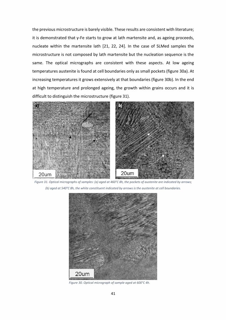
41
the previous microstructure is barely visible. These results are consistent with literature;
it is demonstrated that γ-Fe starts to grow at lath martensite and, as ageing proceeds,
nucleate within the martensite lath [21, 22, 24]. In the case of SLMed samples the
microstructure is not composed by lath martensite but the nucleation sequence is the
same. The optical micrographs are consistent with these aspects. At low ageing
temperatures austenite is found at cell boundaries only as small pockets (figure 30a). At
increasing temperatures it grows extensively at that boundaries (figure 30b). In the end
at high temperature and prolonged ageing, the growth within grains occurs and it is
difficult to distinguish the microstructure (figure 31).
Figure 31. Optical micrographs of samples: (a) aged at 460°C 8h, the pockets of austenite are indicated by arrows;
(b) aged at 540°C 8h, the white constituent indicated by arrows is the austenite at cell boundaries.
Figure 30. Optical micrograph of sample aged at 600°C 4h.

42
Figure 32. SEM micrographs of samples aged at temperature and time: 460°C 8h (a), 490°C 4h (b), 540°C 1h (d),
540°C 8h (d), 600°C 10min (e) and 600°C 4h (f).

43
Austenite starts to nucleate at cell boundaries. This phenomenon can be attributed to
three factors. The first factor involves diffusional processes that are accelerated by
defects, namely grain boundaries. The second factor rely on the similarity between SLM
processed metal microstructure and weld metal microstructure. Because of the fast
cooling of the melted weld metal, elemental segregation at the cellular grain boundary
occurs. Such segregation lowers austenite transformation start temperature (As) [22].
Since there is higher content of Ni at cell boundaries, As in that region is lower, thus γ-
Fe appears earlier. The third factor is the presence of retained austenite at cellular
boundaries in AB samples; the energy needed to have heterogeneous nucleation on it is
lower than that needed to nucleate a new pocket [23].
The SEM micrographs were analysed to obtain the phase balance and to provide a
comparison with the quantitative phase analysis performed with Rietveld method. The
results are listed in table 15.
Table 15. Phases balance from chromatic analysis.
Martensite (%) Austenite (%)
As build 90,7 9,3
460°C 8h 81,2 18,8
490°C 4h 82,8 17,2
540°C 1h 79,6 20,4
540°C 8h 80,8 28,7
600°C 10 min 71,3 19,2
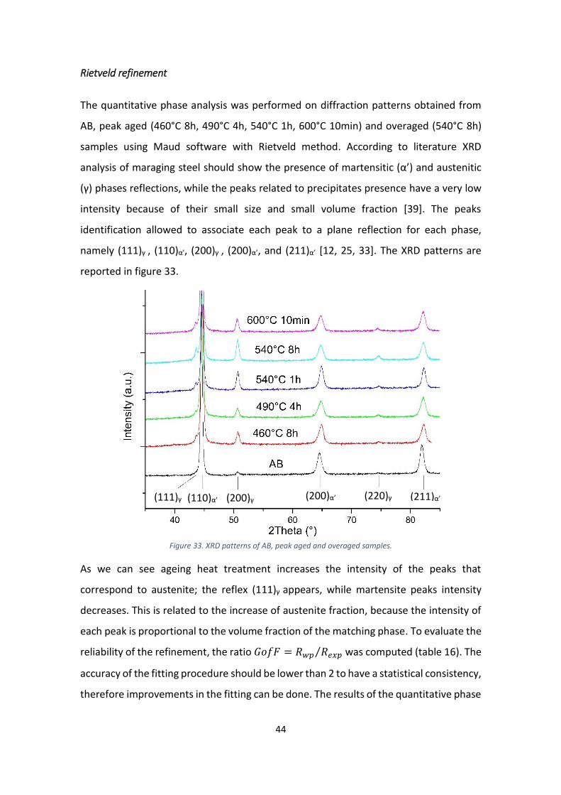
44
Rietveld refinement
The quantitative phase analysis was performed on diffraction patterns obtained from
AB, peak aged (460°C 8h, 490°C 4h, 540°C 1h, 600°C 10min) and overaged (540°C 8h)
samples using Maud software with Rietveld method. According to literature XRD
analysis of maraging steel should show the presence of martensitic (α’) and austenitic
(γ) phases reflections, while the peaks related to precipitates presence have a very low
intensity because of their small size and small volume fraction [39]. The peaks
identification allowed to associate each peak to a plane reflection for each phase,
namely (111)γ , (110)α’, (200)γ , (200)α’, and (211)α’ [12, 25, 33]. The XRD patterns are
reported in figure 33.
As we can see ageing heat treatment increases the intensity of the peaks that
correspond to austenite; the reflex (111)γ appears, while martensite peaks intensity
decreases. This is related to the increase of austenite fraction, because the intensity of
each peak is proportional to the volume fraction of the matching phase. To evaluate the
reliability of the refinement, the ratio 𝐺𝑜𝑓𝐹 = 𝑅𝑤𝑝 𝑅𝑒𝑥𝑝⁄ was computed (table 16). The
accuracy of the fitting procedure should be lower than 2 to have a statistical consistency,
therefore improvements in the fitting can be done. The results of the quantitative phase
(111)γ (110)α’ (200)γ (200)α’ (220)γ (211)α’
Figure 33. XRD patterns of AB, peak aged and overaged samples.

45
analysis and a comparison with the result of chromatic analysis are listed in table 16 and
figure 34.
Table 16. Rietveld refinement results.
Martensite (%) Austenite (%) GofF
As build 88,7 11,3 2,33
460°C 8h 84,5 15,5 2,06
490°C 4h 83,9 16,1 1,81
540°C 1h 82,8 17,2 2,25
540°C 8h 78,7 21,3 1,90
600°C 10 min 82,9 17,1 1,65
These data show a high increase of austenite volume fraction resulting from the ageing.
As expected the γ-Fe fraction grows with temperature and time. Literature reports
similar fractions of austenite at similar temperatures [25]. It is notable that also the AB
sample contains a fraction of γ-Fe. The presence of austenite in as build samples was
also reported by Kempen et al. [33]. On the contrary in solubilized steels the γ-Fe content
is so low to be considered as negligible.
Figure 34. Rietveld refinement and chromatic analysis results comparison.

46
3.2.3 Tensile test
In order to have a deeper understanding of the influence of ageing temperature on
mechanical properties, tensile tests were performed on AB and aged specimens at room
temperature. The influence of porosity and defects on the achievable strength and
elongation is also considered. The correlation between reverted austenite fraction and
the mechanical properties is investigated.
At first vertically (V) and horizontally (H) oriented specimens were compared. Tests on
AB and 460°C-8h samples, that is the peak aged condition at 460°C, provide the following
results (figure 35). As we can see V samples show worse performances than H samples
in both conditions. Only a stress-strain curve corresponding to V samples is shown in
figure 35b because of the premature failure of the other tested specimens. Lower
elongation and lower tensile strength are attributed to the orientation of the layer with
respect to the loading direction [32].
The production technique causes a preferential position of defects. Porosity and melting
defects are more likely found at the interface among different layers hence aligned on
the horizontal plane. In vertical samples the loading direction is orthogonal to the layer
surfaces, while in horizontal ones it is parallel to them. Since defects are placed
orthogonal to the loading direction in V samples, they can lead to cross section
reduction. However it should be noted that porosity causes earlier failure and scattering
of results in all tested conditions.
a) b)
Figure 35. Stress-strain curves of as build (a) and aged (b) samples, horizontally and vertically aligned.
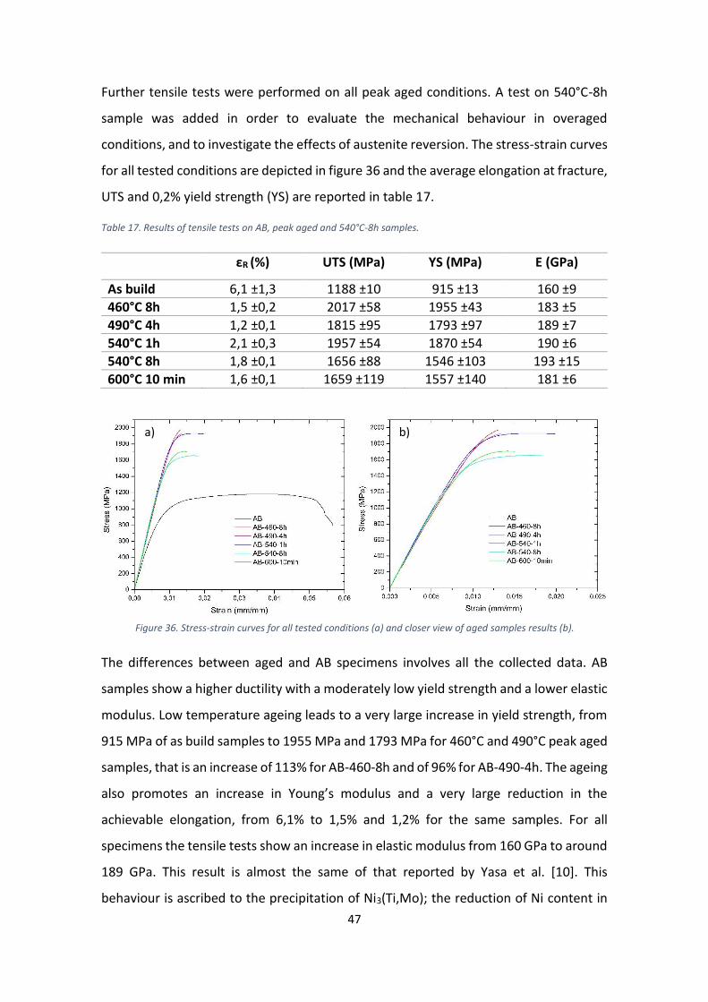
47
Further tensile tests were performed on all peak aged conditions. A test on 540°C-8h
sample was added in order to evaluate the mechanical behaviour in overaged
conditions, and to investigate the effects of austenite reversion. The stress-strain curves
for all tested conditions are depicted in figure 36 and the average elongation at fracture,
UTS and 0,2% yield strength (YS) are reported in table 17.
Table 17. Results of tensile tests on AB, peak aged and 540°C-8h samples.
εR (%) UTS (MPa) YS (MPa) E (GPa)
As build 6,1 ±1,3 1188 ±10 915 ±13 160 ±9
460°C 8h 1,5 ±0,2 2017 ±58 1955 ±43 183 ±5
490°C 4h 1,2 ±0,1 1815 ±95 1793 ±97 189 ±7
540°C 1h 2,1 ±0,3 1957 ±54 1870 ±54 190 ±6
540°C 8h 1,8 ±0,1 1656 ±88 1546 ±103 193 ±15
600°C 10 min 1,6 ±0,1 1659 ±119 1557 ±140 181 ±6
The differences between aged and AB specimens involves all the collected data. AB
samples show a higher ductility with a moderately low yield strength and a lower elastic
modulus. Low temperature ageing leads to a very large increase in yield strength, from
915 MPa of as build samples to 1955 MPa and 1793 MPa for 460°C and 490°C peak aged
samples, that is an increase of 113% for AB-460-8h and of 96% for AB-490-4h. The ageing
also promotes an increase in Young’s modulus and a very large reduction in the
achievable elongation, from 6,1% to 1,5% and 1,2% for the same samples. For all
specimens the tensile tests show an increase in elastic modulus from 160 GPa to around
189 GPa. This result is almost the same of that reported by Yasa et al. [10]. This
behaviour is ascribed to the precipitation of Ni3(Ti,Mo); the reduction of Ni content in
Figure 36. Stress-strain curves for all tested conditions (a) and closer view of aged samples results (b).
a) b)

48
the martensitic matrix may lead to such an increase. The mechanical properties of
samples, aged in the right interval of temperature (460°C 8h, 490°C 4h, 540°C 1h), are
similar to wrought maraging 300 apart from ductility which is reduced in all conditions.
The presence of an increasing austenite fraction may lead to a growth of ductility and
toughness together with a decrease in yield strength and UTS, as reported in literature
[21, 22, 37]. Specifically, Viswanthan et al. [21] studied a wrought 350 maraging steel
and reported that austenite reversion causes a decrease strength and an increment in
elongation and impact toughness. However the increase occurs only in the first stages
of overageing, because coarsening and extensive austenite reversion reduce all
mechanical properties as time proceeds. In order to evaluate the effect on studied
specimens, yield strength and elongation at fracture of each tested specimen were
plotted versus the austenite fraction, as depicted in figure 37.
The ductility reduction is a characteristic of aged maraging steels [9, 38], and it is related
to the strengthening of the matrix because of the presence of precipitates. However the
fracture elongation of selective laser melted components is quite lower than the
elongation of wrought maraging steels both in as build and aged samples [41]. The low
ductility of aged specimens is consistent with literature and datasheet that reports
fracture elongation between 1,5% and 2% [10, 32, 42]. The austenite effect on
elongation seems negligible, all aged specimen elongations are in a small range of values
irrespectively to austenite content (figure 37a). The presence of porosity and melting
faults, that are typical defects in SLM processed parts, along with the intrinsically brittle
full-strength aged matrix are considered to explain such a reduction. Indeed big voids
Figure 37. Elongation (a) and yield strength (b) plotted against austenite fraction.
a) b)

49
and unmolten particles are distributed in the tested specimens as we can see in fracture
surfaces. They cause early failure of specimens so that the austenite effect be barely
seen: the overaged specimen (540°C 8h, 21,3% γ-Fe) shows a mean elongation of 1,8%,
close to the value 1,5% of the low temperature peak aged sample (460°C 8h, 15,5% γ-
Fe). The effect on yield strength is less clear because the reduction in strength is ruled
not only by the austenite content. The total effect of ageing is a combination of softening
and hardening mechanisms which cannot be fully separated. The precipitation of
strengthening intermetallic compounds, the austenite reversion and the coarsening and
embrittlement of the alloy in overageing contribute to the final performance.
γ-Fe effect was not the expected from what is reported in literature. It is one of the
causes of strength loss in the studied samples, but its influence on the ductility is limited
with respect to strengthening mechanisms and to precipitate coarsening. Therefore SLM
processed components show a strength ruled mainly by precipitation hardening and a
ductility governed mainly by defects and precipitates coarsening.
3.2.4 Fracture analysis
The failure mode is examined by means of SEM and optical analysis on fracture surfaces
and sectioned broken samples, respectively. The lack of ductility caused by the ageing
treatment shown in tensile tests was confirmed by the fractographies. On the contrary
specimens without ageing show ductile fracture with extensive plastic deformations.
The difference is well visible in figure 38. It is also clear from figure 38(b) that the fracture
of this specific specimen orginated from a rather large defect, highlighted by the arrow.
Figure 38. AB (a) and 460°C 8h aged (b) fracture surfaces.

50
The ductile failure mechanism consists in nucleation, growth and coalescence of micro
voids that arise where there are precipitates or defects, and the fracture surface is
characterised by the presence of many dimples. These characteristics are visible in SEM
fractographies of AB samples. Cavities between scan tracks, unmelted powder particles
and splats are the defects that can be found (arrows in figure 39a). As regards the brittle
failure, nucleation sites are the same of ductile failure. The fracture mode is different,
the brittle mechanism of fracture growth in the aged samples which has a very low
extent of plastic deformation, mainly developed by cleavage decohesion (figure 39b).
The AB and aged sample were also longitudinally sectioned in order to examine the
profile intersecting the fracture surface. Figure 40a shows that close to the fracture
profile of AB samples, delamination of scan tracks can be identified; it is supposed that
during the loading the crack develops easily along these track boundaries because they
are regions of preferential defect accumulation. Figure 40b shows the aged sample
section. It displays that the amount of plastic deformation is small, and that the fracture
occurs by limited modification of the original cellular shape.
Figure 39. High magnification micrographs of fracture surface of AB (left) and aged(right) samples.

51
Figure 40. SEM micrographs depicting fracture line of AB (a) and aged (b) samples.

52
3.3 DEFECTS ANALYSIS
The presence of defects is an important issue because it prevents the achievement of
full density and affects the mechanical properties, lowering the performance of SLM
processed specimens. Parallel- and perpendicular-to-layer sections were analysed to
evaluate the causes of defect generation. An investigation on the amount of geometrical
irregularities found on as build top surfaces that could possibly affect the deposition and
consolidation of the subsequent layers, their dimensions and has been performed.
Particularly it was investigated the role of the argon flow direction and powder
dispenser direction on the defects distribution. In addition, a dimensional analysis was
performed on as received powder and on powder collected around the base plate. This
powder was affected by the laser beam because it came from the melt pool but was not
embedded in the consolidated layers. This study was carried out to assess the origin of
particles that generate defects.
3.3.1 Section analysis
Stereoscope imaging show a widespread presence of porosity (bright) in both parallel
and perpendicular sections. It is notable that the statement made before about the
preferential disposition of defects among layer boundaries is true as depicted in figure
41. In the parallel-to-layer sections the pores have larger sizes than those in the
perpendicular-to-layer section. The optical analysis and the fractography allowed to
obtain a complete description of the different kinds of defects created during SLM
process.
Figure 41. Spectroscope picture of sections parallel (a) and perpendicular (b) to layers.
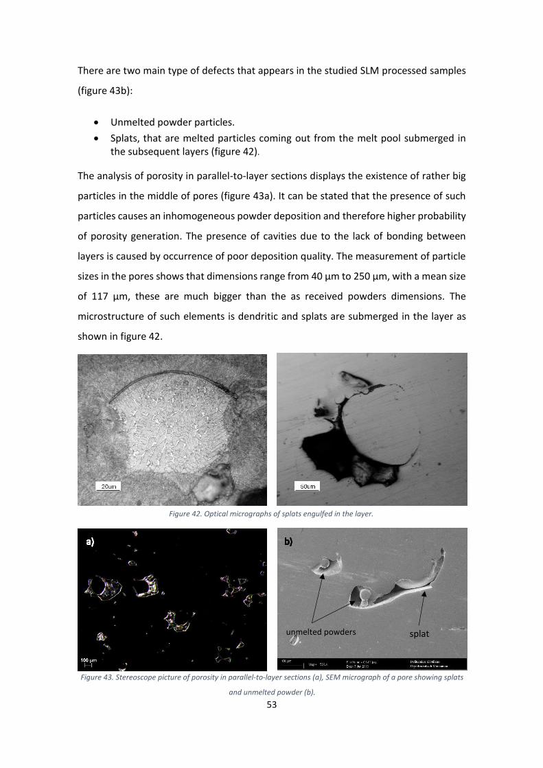
53
There are two main type of defects that appears in the studied SLM processed samples
(figure 43b):
Unmelted powder particles.
Splats, that are melted particles coming out from the melt pool submerged in the subsequent layers (figure 42).
The analysis of porosity in parallel-to-layer sections displays the existence of rather big
particles in the middle of pores (figure 43a). It can be stated that the presence of such
particles causes an inhomogeneous powder deposition and therefore higher probability
of porosity generation. The presence of cavities due to the lack of bonding between
layers is caused by occurrence of poor deposition quality. The measurement of particle
sizes in the pores shows that dimensions range from 40 µm to 250 µm, with a mean size
of 117 µm, these are much bigger than the as received powders dimensions. The
microstructure of such elements is dendritic and splats are submerged in the layer as
shown in figure 42.
Figure 43. Stereoscope picture of porosity in parallel-to-layer sections (a), SEM micrograph of a pore showing splats
and unmelted powder (b).
Figure 42. Optical micrographs of splats engulfed in the layer.
unmelted powders splat

54
By looking at fractographs the presence of unmolten powder particles in the pores and
splats that have a rather bigger size are depicted in figure 44. Splats and powders are
indicated by arrows. It seems that splats are the main cause of porosity in studied
samples, they are suggested to be the reason of big pores in which we can see unmolten
particle presence.
3.3.2 Powder characterization
SEM analyses were performed on powders to evaluate the effect of laser melting
process on them and to compare them with the defects found in specimens. Two
different kinds of powders were analyzed: as received powders and powders collected
out from the base plate after processing. The second type of powders is made up of
splats that came from the melt pools and are blown away from it by the argon gas flow.
Figure 46 depicts the building camera of the used Renishaw AM250 system, it is specified
the area of powder collection and the direction of the argon flux.
SEM images show the shape and solidification structure of both powders groups. As
regards the shape, the processed particles are bigger and more spherical than the as
received ones. The blown particle are affected by heat in such an extent to cause melting
and coarsening. The different morphologies at the same magnification are shown in
figure 47.
Figure 44. SEM fractographs of AB (left) and aged (right) specimen showing splats and unmolten powder.

55
All powders present dendrites as shown by micrographs of figure 45; the optical
micrograph of an unmelted particle in a pore is reported, it has the same microstructure
of collected powder. The cause of this microstructure can be ascribed to the cooling rate
resulting from the powder production method in case of as received powders and from
the blowing in case of collected powders.
Figure 47. Morphology of as received particles (left) and collected particles (right).
Figure 45. SEM micrograph of as received powders (left) and optical micrograph of a pore particle (right).
Figure 46. Picture of the building camera during SLM process

56
In order to evaluate the changes in size distribution, pictures as in figure 48 were
analyzed with the software ImageJ for image analysis. Through this program it was
possible to estimate the statistics about particle diameters by using two approximations:
(i) all particles were reduced to their 2D projection, then projections areas were
computed; (ii) diameters were obtained by considering all projections as circular.
The results of this computation are summarized in table 18 and figure 49. They show
how the processed-particle size increases: minimum, maximum and mean diameter rise
and the distribution peak shifts towards higher dimensions and becomes sharper. It
difficult to find particles smaller than 20 µm in the collected powder. Since the collected
powders present a different distribution with bigger particles, it can be stated that they
may act as starting points for defect generation, being them larger than the layer
thickness. By comparing the defect sizes with the sizes of the particles in the pores, it
appears that they are smaller in the average. The cause is that the collected particles are
Figure 48. Scheme of the first approximation: backscattered electron micrograph (left) transformed in 2D image
(right).
Figure 49. Cumulative (left) and relative (right) frequency (%) of studied powders.

57
the smaller ones because the bigger blown particles are supposed not to be able toreach
long distances from the molten pool.
Table 18. Diameter changes in as received and collected powders.
Mean diameter (µm)
Minimum diameter (µm)
Maximum diameter (µm)
As received powder 24,31 5,24 59,70 Collected powder 35,01 7,17 83,78
3.3.3 As built top surfaces analysis
In order to have a better understanding of the defect generation process the as built top
surfaces of samples were analysed, and the same approximations used for powder size
measurement was applied. The aim was to extend the analysis performed on collected
powders and pores and to validate two hypotheses:
The particles on layer surfaces are the same that were found in the pores.
The defect quantity and sizes show a trend ruled by gas flow direction and
powder dispenser direction
At first an investigation on a small area was carried out. An example of analysed SEM
images is shown in figure 50 and 51. There is a distribution of particles weldedon the top
surface in addition to the evidence of the scanning lines. Particles consists in small
unmolten powders and bigger splats of various dimensions.
Figure 50. SEM image at high magnification of as built top
surface.

58
By comparing the obtained results with the results of the collected powders, it is verified
that the bigger particles fall near to the melt pool. The relative frequency graph in figure
52b shows the possibility to find rather big particles (>90 µm) on scan tracks; such a
dimension is not found in collected powders. The measurements carried on the parallel
to layer section showed the presence of big particles that are in the same size range of
those found on top surfaces. The difference is that the pores contain more large particles
than the number found on unmodified layer surfaces Because the smaller are likely
melted during the scanning of the above layer.
b) a)
Figure 51. SEM image of as built top surface.
Figure 52. Cumulative (a) and relative (b) frequency of particle sizes found in collected powders, pores and as built
top surfaces.

59
Trends in defect distribution
Analysis of the porosity revealed a dependency on the position of samples over the
building plate. The amount of defects was found to increase diagonally with respect to
the base plate according to the direction of gas flow and powder dispenser direction. To
evaluate the effect of the single transport contribution two series of samples, consisting
in three 20mm×60mm surfaces, aligned as depicted in figure 53, were analysed. Samples
were designated with an increasing number from the “origin” to the plate border. Each
surface was divided into smaller areas of 5 mm × 4 mm, obtaining 4 rows and 15 columns
(figure 54). These areas were alternatively chosen and processed using Photoshop to
isolate splats and particles and then analysed to measure their diameters. Then the
number and the diameter of particles in each area was computed and the total particle
number and mean particle diameter for each column was plotted against the respective
investigated direction. Therefore the following graphs were obtained, as depicted in
figure 55.
Figure 54. Scheme of samples surface partition and of analysed areas.
Gas flow direction (x)
Po
wd
er pro
vider d
irection
(y)
Porosity
Figure 53. Scheme of the base plate with studied samples.
1
2
3
4 5 6

60
The result of the analysis shows that even if a trend within all the samples does not
clearly appears, the overall behaviour is evident when considering the trend line. In both
directions the number of particle increases as the distance from the origin increases
(figure 55a, 55c). This result was expected because, as seen before the particles are
blown away from the melt pool by the argon flow. So it is likely to found an increasing
number of blown particles as we move toward the border of the base plate. The effect
of the powder delivery position is less evident. In order to deposit the powder it moves
over the baseplate and it probably drags large particles along its path. This is confirmed
by the particle diameters which grows with increasing distance (figure 55b). As regards
the blown particle dimensions, the data confirm the results reported before. The size is
found to decrease along the direction of gas flow (figure 55d). This means that only small
particles can reach long distances from the melt pool as we can see also in the size
distributions of collected powders and on top surfaces.
Figure 55. Particle number along powder supplier direction (a), toward gas flow (c) and particle diameter along
supplier direction (b), gas flow direction (d).
a) b)
c) d)
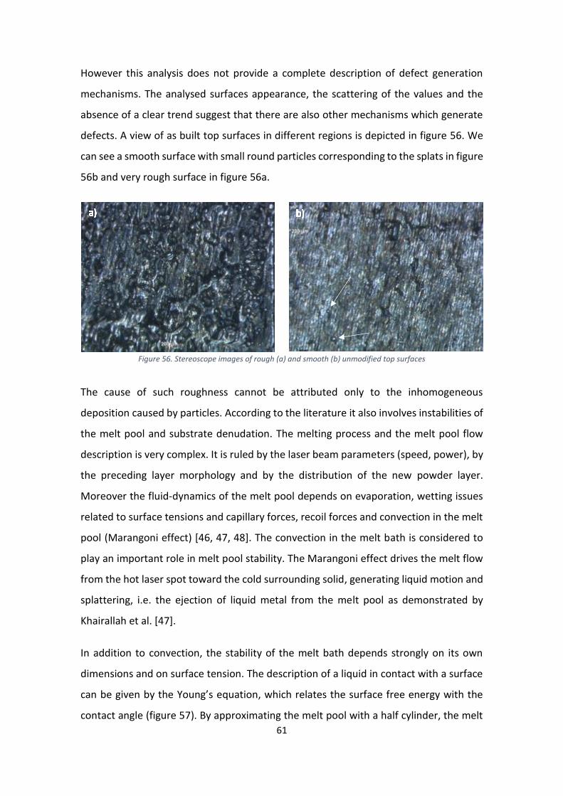
61
However this analysis does not provide a complete description of defect generation
mechanisms. The analysed surfaces appearance, the scattering of the values and the
absence of a clear trend suggest that there are also other mechanisms which generate
defects. A view of as built top surfaces in different regions is depicted in figure 56. We
can see a smooth surface with small round particles corresponding to the splats in figure
56b and very rough surface in figure 56a.
The cause of such roughness cannot be attributed only to the inhomogeneous
deposition caused by particles. According to the literature it also involves instabilities of
the melt pool and substrate denudation. The melting process and the melt pool flow
description is very complex. It is ruled by the laser beam parameters (speed, power), by
the preceding layer morphology and by the distribution of the new powder layer.
Moreover the fluid-dynamics of the melt pool depends on evaporation, wetting issues
related to surface tensions and capillary forces, recoil forces and convection in the melt
pool (Marangoni effect) [46, 47, 48]. The convection in the melt bath is considered to
play an important role in melt pool stability. The Marangoni effect drives the melt flow
from the hot laser spot toward the cold surrounding solid, generating liquid motion and
splattering, i.e. the ejection of liquid metal from the melt pool as demonstrated by
Khairallah et al. [47].
In addition to convection, the stability of the melt bath depends strongly on its own
dimensions and on surface tension. The description of a liquid in contact with a surface
can be given by the Young’s equation, which relates the surface free energy with the
contact angle (figure 57). By approximating the melt pool with a half cylinder, the melt
Figure 56. Stereoscope images of rough (a) and smooth (b) unmodified top surfaces

62
pool becomes instable and balling effect occurs when the total surface of the pool
becomes larger than that of a sphere with the same volume. Thus the melt bath should
have a length-to-diameter ratio as small as possible [5]. Because of this phenomenon,
balling can occur also when the environmental conditions are controlled and the
substrate is not oxidized.
Substrate denudation refers to coalescence of powders that do not reach the melt pool.
The laser beam interacts with the powder and with the substrate that can be the base
plate or the previously processed layer. The energy provided by the laser heats the
powder and the underlying surface. The heat leads to the formation of the track but it
is also conducted through the substrate causing sintering and melting of near the scan
line. The denudation zone is the zone around the track where the powders have a lower
density [46, 47]. The subsequent scan tracks will find a lower amount of powders and
inhomogeneous distribution, so they may generate defects. Another issue is the
formation of satellites, remelted particles partially linked to the track that could cause
porosity. They are produced by melt splattering and partial powder melting near the
scan track [31]. The extensive presence of satellites was found during the surface
analysis of lattices created by SLM on the same maraging steel, as reported in appendix
5.1 (figure 58), so it can be considered a possible cause of porosity also during bulky
parts production.
Figure 57. Young’s equation (a) and balling effect (b) scheme [5].

63
To summarize the origin of such defects is attributed to the SLM system configuration
(gas flow direction and powder dispenser direction) by the analysis of blown powder
and unmodified top surfaces. Moreover it can be stated that the roughness arises also
from the used process parameters, mainly laser beam power and speed. They are
additional sources of porosity because they strongly influence the tracks morphology
and the fluid-dynamics of the melt pool. The final porosity will be an overall contribution
of all these defect-generating mechanisms.
4 CONCLUSIONS
Selective laser melting (SLM) technique was used to process a 18Ni-300 maraging steel
(1.2907). This processing method is an additive manufacturing technique that consist in
melting and consolidating micrometric metal powders into solid layers by means of a
laser beam. The produced parts are made of a sequence of metallic layers composed of
a series of overlapped scan tracks that bounds metallurgically one over the other.
Maraging steels are age-hardenable alloys with a low-carbon and high-nickel martensitic
matrix. Their usual heat treatment sequence involves at first a solution treatment in fully
austenitic region, followed by quenching and an ageing treatment at lower temperature.
The ageing treatment temperatures and times are very important for the achievable
strength. Strengthening precipitation of Ni3(Ti,Mo) can occur. Additional softening
Figure 58. Satellites presence on lattice structures.

64
mechanisms due to coarsening of precipitates and austenite reversion is recorded on
overageing.
Since SLM technique is an atypical processing method which involves high cooling rates
of the melt pool and the superposition of many layers, the microstructure of as build
(AB) samples is very different with respect to common solution treated wrought
maraging steels. Micrographs of AB samples made evident the additive procedure and
the high cooling rates influence. Scan track boundaries and melt pools were visible; the
microstructure was made of cells with size lower than1 µm and exhibited epitaxial
growth among scan line boundaries. Some SLM parts were subjected to solution
treatment (SOL) to assess the microstructural modifications of such a heat treatment.
SOL samples microstructure was completely different form the AB one. It was composed
by fairly coarse laths of martensite, much coarser than the AB cells. EBSD analysis on
SOL showed the presence of retained austenite at grain boundaries.
A comparison between solution treated and as build samples was carried out in order
to evaluate the differences in ageing sequence and in mechanical properties given by
the different microstructures. Kinetic analysis of precipitation was performed using
differential scanning calorimetry tests. The resulting DSC curves showed two exothermic
peaks corresponding to precipitation and two endothermic peaks corresponding to
austenite reversion. The similarity between DSC curves and computed enthalpies of AB
and SOL samples suggested small differences in the ageing sequence. AB samples
showed a lower activation energy than SOL samples because of the finer microstructure
that enhances diffusion. Ageing tests presented a quite similar behavior, peak hardness
was reached in the same time at the same temperatures. The only difference appears in
non-aged samples likely because the Hall-Petch strengthening given by the finer
microstructure of AB samples (371 HV vs 279 HV) was partially lost after solution
treatment. Tensile test results showed that solution treatment has a detrimental effect
on mechanical properties both in non-aged, and in peak aged conditions. AB samples
presented a higher work hardening ability and higher yield strength in all ageing
conditions because of the finer microstructure.

65
Since the solution treated samples were proved to have lower performance and
therefore convenience, only AB samples were subjected to further investigation. Ageing
tests were performed at temperatures in the ASTM advised ageing temperature range
(450-510°C) and at higher temperatures. Ageing times and high temperatures were
extended to study overageing behavior, to stimulateaustenite reversion and to evaluate
its influence on mechanical properties. Isothermal ageing curves reported a decreasing
hardness peak which occurs at shorter times as temperature increases. This
phenomenon is due to the enhancement of diffusion by temperature which causes the
simultaneous occurrence of strengthening and softening mechanisms. The loss of
strength in overageing at high temperature is more pronounced than that found in low
temperature ageing, owing to massive precipitates coarsening and austenite reversion.
The microstructural characterization was performed on all peak aged and an overaged
AB samples to study the austenite reversion. Austenite was present in all conditions; the
reversion occurs firstly at cell boundaries and then, for the longest ageing times, within
the cells. Image analyses based on SEM micrographs and quantitative phase analysis
using Rietveld refinement method on XRD patterns allowed to obtain the austenite
volume fraction for the investigated samples. As expected, they exhibited an increasing
content of γ-Fe for increasing time and temperature. Tensile tests on peak aged and
overaged samples were performed. The obtained yield strength, UTS and elastic
modulus are similar to those reported for wrought maraging steels with the exception
of fracture elongation. Even if it was reported in literature an increment of elongation
with increasing austenite fraction, in the preset investigation the influence of γ-Fe on
fracture elongation was found to be almost negligible. Thus the reason of such a
reduction of elongation can be attributed to the high sample porosity and to the matrix
embrittlement due to marked strengthening. As regards the γ-Fe effect on yield
strength, there is noclear correlation between the decreasing strength and the
increasing amount of austenite content. This is because during ageing the reversion
occurs along with other softening mechanisms. It seems that austenite has a lower
softening effect than coarsening of precipitates. Fracture analysis showed ductile
fracture behavior of AB samples with dimples creation and brittle fracture mode of aged
samples with cleavage decohesion.

66
In the end, an analysis on defects found in SLM processed parts was performed. The
reason of this analysis were the results of tensile tests and of the fracture analysis.
Tensile tests on samples with different layer orientation with respect to loading
direction allowed to find the preferential site of porosity generation, the interlayer
boundary. The fractographic analysis show that porosity is the main cause of nucleation
of cracks and early failure. Analyses on samples section, on powders and on as built top
surfaces showed that splats, particles blown away by gas flow from the melt pool, are
one of the main type of defects at the origin of porosity. Other results of the analysis of
SLM surfaces were that the splats number increases along the gas flow direction and
the powder dispenser motion direction, while their dimension decreases along gas flow
direction and increases along dispenser motion direction. Another cause of porosity was
identified in the instability of the melt pool, probably caused by wrong process
parameters (laser beam power and speed).

67
5 APPENDIX
5.1 LATTICE MICROSTRUCTURE
SLM process allows to produce both massive parts and complex structures with small
features. To evaluate the effect of laser melting on small structures, BCC lattices were
produced and analysed through optical and SEM microscopy. Lattices were not solution
treated. Small and high magnification view of such lattices is reported in figure 59.
These images show an extensive presence of satellites, i.e. powder particles which sinter
and metallurgically join with the scan tracks. This effect is clearer in sections of the
lattices; the dendritic structure of satellites confirms that the powders stick to the scan
tracks (figure 60). This phenomenon is more visible when the tracks create a new surface
and does not lay on the preceding layers.
Figure 59. Low magnification (left) and high magnification (right) SEM images of a BCC lattice.
Figure 60. SEM (left) and section optical micrograph (right) showing the dendritic structure of satellites.

68
Lattice sections also provide an example of the influence of cooling rate on grains
dimensions (figure 61). The bottom of the piece was in contact only with the powder
bed, so its cooling rate was slower with respect to the subsequent layers. It is easy to
see that the microstructure becomes finer as the solid part becomes larger, i.e. the
solidification is more rapid. However the lattices microstructure is the same of as build
microstructure, consisting in fine cellular colonies.
5.2 AGEING OF AB AND SOL SAMPLES AT 460°C AND 490°C
Table 19.Hardness values of AB and SOL samples aged at 460°C.
AB-460°C SOL-460°C
Ageing time Hardness (HV) Std. Dev. Hardness (HV) Std. Dev.
Non aged 371,05 12,85 279,58 8,37
30 min 483,96 15,97 484,7 10,61
1 h 539,9 13,16 524,95 10,07
2 h 560,02 12,35 551,56 10,41
3h 579,56 10,30 564,44 9,87
4h 600,48 10,60 582,71 6,59
6h 603,64 13,46 591,18 8,11
8h 632,41 4,654 613,6 11,09
12h 610,74 8,36 589,15 7,14
16h 611,78 7,79 595,11 12,83
24h 607,53 7,39 589,58 5,77
2 day 620,84 4,84 618,07 5,18
5 day 595,38 6,24 594,17 6,82
10 day 588,18 5,13 602,11 3,23
14 day 586,6 4,07 585,17 7,66
Figure 61.Oprical micrograph of AB lattice sample.

69
Table 20. Hardness values of AB and SOL samples aged at 490°C.
AB-490°C SOL-490°C
Ageing time Hardness (HV) Std. Dev. Hardness (HV) Std. Dev.
Non aged 371,05 12,8 279,58 8,37
30 min 562,85 6,53 554,82 3,85
1 h 565,94 5,08 581,27 5,98
2 h 590,96 4,24 596,23 6,35
3h 604,35 5,32 607,11 2,88
4h 607,75 4,70 616,07 6,22
6h 594,68 3,36 611,76 5,52
8h 599,62 5,67 609,5 6,89
12h 600,28 4,51 600,37 4,15
5.3 AGEING OF AB SAMPLES AT 540°C AND 600°C
Table 21. Hardness values of AB samples aged at 540°C and at 600°C.
AB-540°C AB-600°C
Ageing time Hardness (HV) Std. Dev. Hardness (HV) Std. Dev.
Non aged 371,0563 12,854 371,0563 12,854
5 min 478,1429 5,744811 530,4857 7,434924
10 min 530,8286 7,736001 537,2429 5,234774
15 min 534,2 4,345496 509,5571 5,035824
30 min 568,4571 6,305515 486,8571 6,302343
1h 582,8429 6,948107 469,9 10,25898
2h 561,5857 3,700643 452,3857 5,13661
3h 567,1429 6,884973 440,9571 3,86258
4h 547,2286 6,523219 438,2286 4,755598
6h 522,9429 5,581474
8h 523,5857 7,040935

70
5.4 Y AND DY/DT VS. T CURVES FOR PRECIPITATION
Figure 63. Y and dY/dT versus temperature curves for peak 1 in AB samples at different heating rates.
Figure 64. Y and dY/dT versus temperature curves for peak 1 in SOL samples at different heating rates.
Figure 62. Y and dY/dT versus temperature curves for peak 2 in AB samples at different heating rates.

71
5.5 ARRHENIUS AND KISSINGER PLOTS FOR PRECIPITATION
Figure 65. Y and dY/dT versus temperature curves for peak 2 in SOL samples at different heating rates.
Figure 66. Arrhenius (left) and Kissinger (right) plots for peak 1 in AB samples.
Figure 67. Arrhenius (left) and Kissinger (right) plots for peak 1 in SOL samples.

72
5.6 Y AND DY/DT VS. T CURVES FOR REVERSION
Figure 70. Y and dY/dT versus temperature curves for peak 3 in AB samples at different heating rates.
Figure 69. Arrhenius (left) and Kissinger (right) plots for peak 2 in AB samples.
Figure 68. Arrhenius (left) and Kissinger (right) plots for peak 2 in SOL samples

73
Figure 73. Y and dY/dT versus temperature curves for peak 4 in SOL samples at different heating rates.
Figure 72. Y and dY/dT versus temperature curves for peak 4 in AB samples at different heating rates.
Figure 71. Y and dY/dT versus temperature curves for peak 3 in SOL samples at different heating rates.
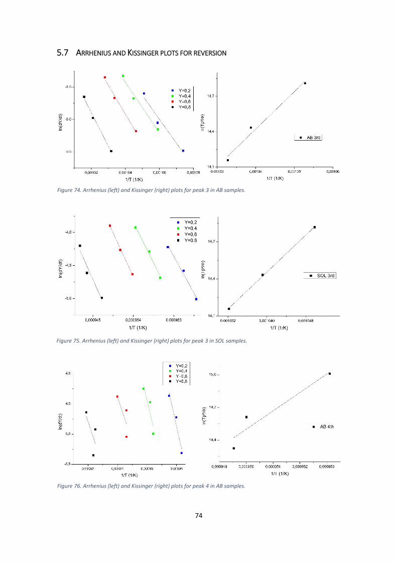
74
5.7 ARRHENIUS AND KISSINGER PLOTS FOR REVERSION
Figure 75. Arrhenius (left) and Kissinger (right) plots for peak 3 in SOL samples.
Figure 74. Arrhenius (left) and Kissinger (right) plots for peak 3 in AB samples.
Figure 76. Arrhenius (left) and Kissinger (right) plots for peak 4 in AB samples.

75
Figure 77. Arrhenius (left) and Kissinger (right) plots for peak 4 in SOL samples.

76
6 BIBLIOGRAPHY
1. Kruth J-, Levy G, Klocke F, Childs THC. Consolidation phenomena in laser and
powder-bed based layered manufacturing. CIRP Annals 2007;56(2):730-59.
2. Kruth J-. Part and material properties in selective laser melting of metals. In: ;
2010. .
3. Casalino G, Campanelli SL, Contuzzi N, Ludovico AD. Experimental investigation
and statistical optimisation of the selective laser melting process of a maraging
steel. Opt Laser Technol 2015;65:151-8.
4. Monroy K, Delgado J, Ciurana J. Study of the pore formation on CoCrMo alloys
by selective laser melting manufacturing process. Procedia Engineering
2013;63:361-9.
5. Kruth JP, Froyen L, Van Vaerenbergh J, Mercelis P, Rombouts M, Lauwers B.
Selective laser melting of iron-based powder. J Mater Process Technol
2004;149(1-3):616-22.
6. Mercelis P, Kruth J. Residual stresses in selective laser sintering and selective
laser melting. Rapid Prototyping Journal 2006;12(5):254-65.
7. Pardal JM, Tavares SSM, Cindra-Fonseca MP, da-Silva MR, Neto JM, Abreu HFG.
Influence of temperature and aging time on hardness and magnetic properties
of the maraging steel grade 300. J Mater Sci 2007;42(7):2276-81.
8. Tewari R, Mazumder S, Batra IS, Dey GK, Banerjee S. Precipitation in 18 wt% Ni
maraging steel of grade 350. Acta Materialia 2000;48(5):1187-200.
9. Leitner H, Schober M, Schnitzer R, Zinner S. Strengthening behavior of Fe–Cr–Ni–
Al–(ti) maraging steels. Materials Science & Engineering.A, Structural Materials:
Properties, Microstructure and Processing 2011;528(15):5264-70.
10. Yasa E. Microstructure and mechanical properties of maraging steel 300 after
selective laser melting. In: ; 2010.
11. Moshka O, Pinkas M, Brosh E, Ezersky V, Meshi L. Addressing the issue of
precipitates in maraging steels – unambiguous answer. Materials Science &
Engineering.A, Structural Materials: Properties, Microstructure and Processing
2015;638:232-9.
12. Hossein Nedjad S, Meimandi S, Mahmoudi A, Abedi T, Yazdani S, Shirazi H, Nili
Ahmadabadi M. Effect of aging on the microstructure and tensile properties of

77
Fe–Ni–Mn–Cr maraging alloys. Materials Science & Engineering.A, Structural
Materials: Properties, Microstructure and Processing 2009;501(1-2):182-7.
13. Levy GN. Rapid manufacturing and rapid tooling with layer manufacturing (LM)
technologies, state of the art and future perspectives. CIRP Annals
2003;52(2):589-609.
14. Jägle E, Sheng Z, Wu L, Lu L, Risse J, Weisheit A, Raabe D. Precipitation reactions
in age-hardenable alloys during laser additive manufacturing. Jom
2016;68(3):943-9.
15. Guo Z. Quantification of precipitation hardening and evolution of precipitates.
Materials Transactions 2002;43(6):1273-82.
16. Ardell AJ. Precipitation hardening. Metallurgical Transactions.A, Physical
Metallurgy and Materials Science 1985;16(12):2131-65.
17. Yadroitsev I, Thivillon L, Bertrand P, Smurov I. Strategy of manufacturing
components with designed internal structure by selective laser melting of
metallic powder. Appl Surf Sci 2007;254(4):980-3.
18. Galindo Nava EI, Rainforth WM, Rivera-Díaz-del-Castillo PEJ. Predicting
microstructure and strength of maraging steels: Elemental optimisation. Acta
Materialia 2016;117:270-85.
19. Pardal JM, Tavares SSM, Terra VF, Da Silva MR, Dos Santos DR. Modeling of
precipitation hardening during the aging and overaging of 18Ni–Co–Mo–Ti
maraging 300 steel. J Alloys Compounds 2005;393(1-2):109-13.
20. Würzinger P, Rabitsch R, Meyer W. Production of maraging steel grades and the
influence of specified and nonspecified elements for special applications. J Mater
Sci 2004;39(24):7295-302.
21. Viswanathan UK, Dey GK, Sethumadhavan V. Effects of austenite reversion
during overageing on the mechanical properties of 18 ni (350) maraging steel.
Materials Science & Engineering.A, Structural Materials: Properties,
Microstructure and Processing 2005;398(1-2):367-72.
22. Yang S, Peng Y, Zhang X, Tian Z. Phase transformation and its effect on
mechanical properties of C300 weld metal after aging treatment at different
temperatures. Journal of Iron and Steel Research(International) 2015;22(6):527-
33.

78
23. Jägle E, Choi P, Van Humbeeck J, Raabe D. Precipitation and austenite reversion
behavior of a maraging steel produced by selective laser melting. J Mater Res
2014;29(17):2072-9.
24. Li X, Yin Z. Reverted austenite during aging in 18Ni(350) maraging steel. Mater
Lett 1995;24(4):239-42.
25. Pardal JM, Tavares SSM, Cindra-Fonseca MP, Abreu HFG, Silva JJM. Study of the
austenite quantification by X-ray diffraction in the 18Ni-co-mo-ti maraging 300
steel. J Mater Sci 2006;41(8):2301-7.
26. Schnitzer R, Radis R, Nöhrer M, Schober M, Hochfellner R, Zinner S, Povoden
Karadeniz E, Kozeschnik E, Leitner H. Reverted austenite in PH 13-8 mo maraging
steels. Mater Chem Phys 2010;122(1):138-45.
27. Guo Z, Sha W, Li D. Quantification of phase transformation kinetics of 18 wt.% ni
C250 maraging steel. Materials Science & Engineering.A, Structural Materials:
Properties, Microstructure and Processing 2004;373(1-2):10-20.
28. Starink MJ. The determination of activation energy from linear heating rate
experiments: A comparison of the accuracy of isoconversion methods.
Thermochimica Acta 2003;404(1-2):163-76.
29. Lutterotti L, Scardi P. Simultaneous structure and size-strain refinement by the
Rietveld method. Journal of Applied Crystallography 1990;23:246-52.
30. Liu H, Kuo C. Quantitative multiphase determination using the Rietveld method
with high accuracy. Mater Lett 1996;26(3):171-5.
31. Yadroitsev I, Krakhmalev P, Yadroitsava I, Johansson S, Smurov I. Energy input
effect on morphology and microstructure of selective laser melting single track
from metallic powder. J Mater Process Technol 2013;213(4):606-13.
32. Kruth J-, Mercelis P, Van Vaerenbergh J, Froyen L, Rombouts M. Binding
mechanisms in selective laser sintering and selective laser melting. Rapid
Prototyping Journal 2005;11(1):26-36.
33. Kempen K, Yasa E, Thijs L, Kruth J-, Van Humbeeck J. Microstructure and
mechanical properties of selective laser melted 18Ni-300 steel. Physics Procedia
2011;12(PART 1):255-63.
34. Menapace C, Lonardelli I, Molinari A. Phase transformation in a nanostructured
M300 maraging steel obtained by SPS of mechanically alloyed powders. Journal
of Thermal Analysis and Calorimetry 2010;101(3):815-21.
79
35. Shekhter A, Aaronson HI, Miller MK, Ringer SP, Pereloma EV. Effect of aging and
deformation on the microstructure and properties of fe-ni-ti maraging steel.
Metallurgical and Materials Transactions A 2004;35(13):973-83.
36. Kapoor R, Batra IS. On the α′ to γ transformation in maraging (grade 350), PH 13-
8 mo and 17-4 PH steels. Materials Science & Engineering.A, Structural Materials:
Properties, Microstructure and Processing 2004;371(1-2):324-34.
37. Schnitzer R, Zickler G, Lach E, Clemens H, Zinner S, Lippmann T, Leitner H.
Influence of reverted austenite on static and dynamic mechanical properties of
a PH 13-8 mo maraging steel. Materials Science & Engineering.A, Structural
Materials: Properties, Microstructure and Processing 2010;527(7-8):2065-70.
38. Ooi SW, Hill P, Rawson M, Bhadeshia HKDH. Effect of retained austenite and high
temperature laves phase on the work hardening of an experimental maraging
steel. Materials Science & Engineering.A, Structural Materials: Properties,
Microstructure and Processing 2013;564:485-92.
39. Guo Z, Sha W. Quantification of precipitate fraction in maraging steels by X-ray
diffraction analysis. Materials Science and Technology 2004;20(1):126-30.
40. Vander Voort GF. Etching isothermally treated steels. 2001.
41. Carpenter Technology Corporation CarTech® NiMark® Alloy 300 datasheet
[Internet]; c2016. Available from: https://www.cartech.com/en/product-
solutions/cartech-nimark-alloy-300/.
42. 3T RPD Ltd maraging steel 1.2907 material specification [Internet]; c2015.
Available from: http://www.3trpd.co.uk/wp-
content/uploads/2015/05/Maraging-Steel-1-2709.pdf.
43. Alavudeen A, Venkateshwaran N, Winowlin Jappes JT. A textbook of engineering
materials and metallurgy. Firewall Media; 2006.
44. Frazier W. Metal additive manufacturing: A review. Journal of Materials
Engineering and Performance 2014;23(6):1917-28.
45. Peretyagin PY, Zhirnov IV, Vladimirov Y, Tarasova TV, Okunkova AA. Track
geometry in selective laser melting. Russian Engineering Research
2015;35(6):473-6.
46. Yadroitsev I, Smurov I. Surface morphology in selective laser melting of metal
powders. Physics Procedia 2011;12(PART 1):264-70.

80
47. Khairallah S, Anderson A, Rubenchik A, King W. Laser powder-bed fusion additive
manufacturing: Physics of complex melt flow and formation mechanisms of
pores, spatter, and denudation zones. Acta Materialia 2016;108:36-45.
48. Bauereiß A, Scharowsky T, Körner C. Defect generation and propagation
mechanism during additive manufacturing by selective beam melting. J Mater
Process Technol 2014;214(11):2522-8.

81
RINGRAZIAMENTI