Microsoft Office 2010

Excel Chapter 1Creating a Worksheet andan Embedded Chart

2

What is Excel• Excel is a spreadsheet program in the Microsoft

Office system. • You can use Excel to create and format workbooks

(a collection of spreadsheets) in order to analyze data and make more informed business decisions.

• Specifically, you can use Excel to track data, build models for analyzing data, write formulas to perform calculations on that data, pivot the data in numerous ways, and present data in a variety of looking charts.

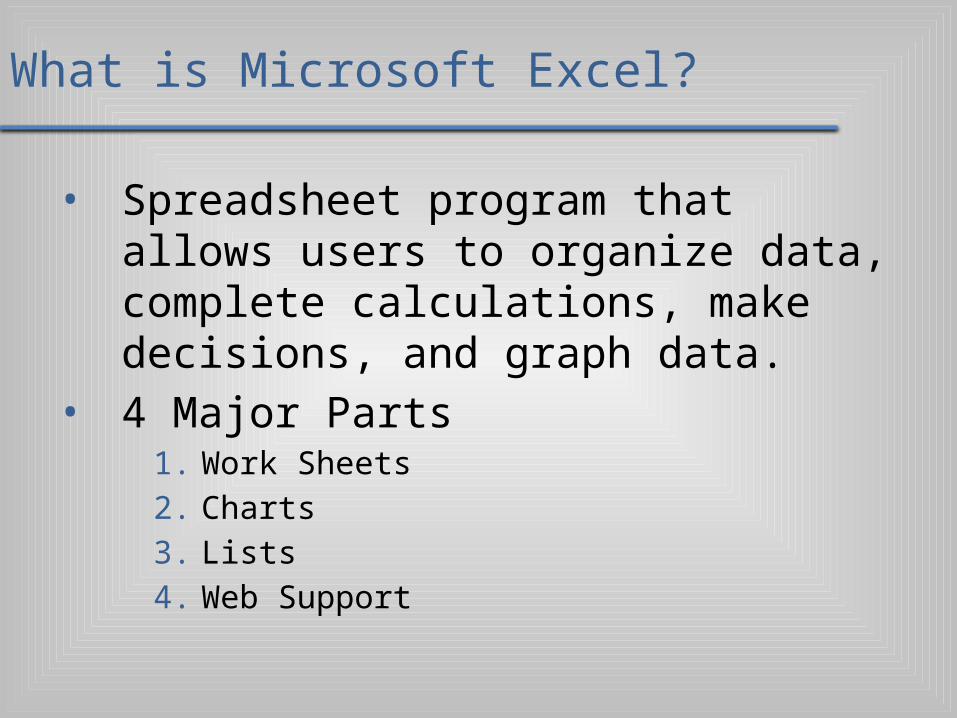
What is Microsoft Excel?

• Spreadsheet program that allows users to organize data, complete calculations, make decisions, and graph data.

• 4 Major Parts1. Work Sheets2. Charts3. Lists 4. Web Support

4

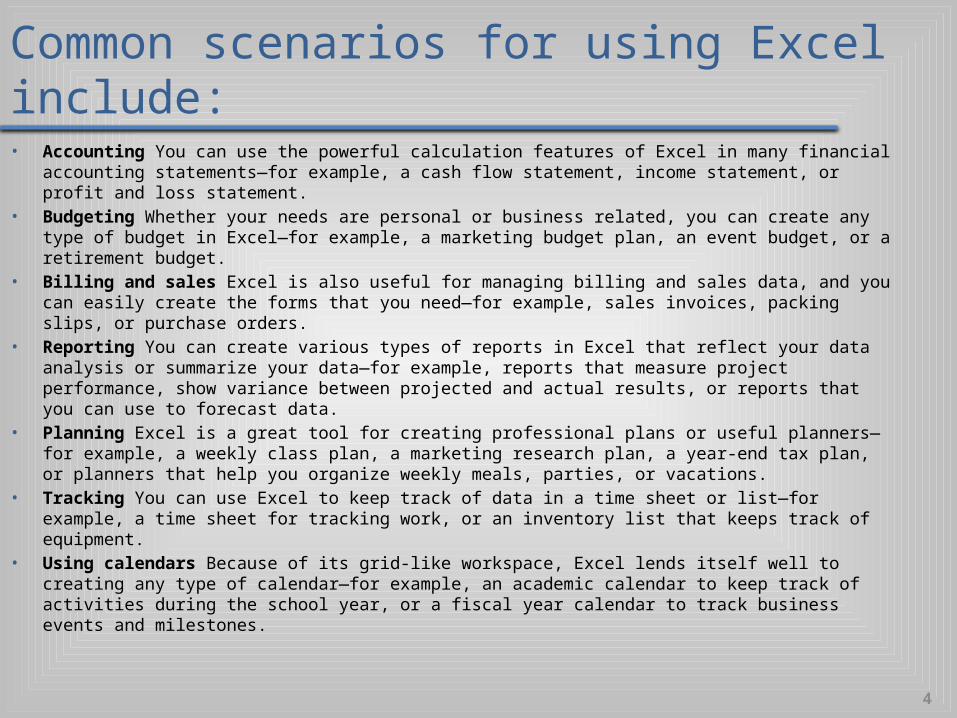
Common scenarios for using Excel include:• Accounting You can use the powerful calculation features of Excel in many financial accounting statements—for

example, a cash flow statement, income statement, or profit and loss statement.• Budgeting Whether your needs are personal or business related, you can create any type of budget in Excel—for

example, a marketing budget plan, an event budget, or a retirement budget.• Billing and sales Excel is also useful for managing billing and sales data, and you can easily create the forms that

you need—for example, sales invoices, packing slips, or purchase orders.• Reporting You can create various types of reports in Excel that reflect your data analysis or summarize your data

—for example, reports that measure project performance, show variance between projected and actual results, or reports that you can use to forecast data.

• Planning Excel is a great tool for creating professional plans or useful planners—for example, a weekly class plan, a marketing research plan, a year-end tax plan, or planners that help you organize weekly meals, parties, or vacations.

• Tracking You can use Excel to keep track of data in a time sheet or list—for example, a time sheet for tracking work, or an inventory list that keeps track of equipment.

• Using calendars Because of its grid-like workspace, Excel lends itself well to creating any type of calendar—for example, an academic calendar to keep track of activities during the school year, or a fiscal year calendar to track business events and milestones.

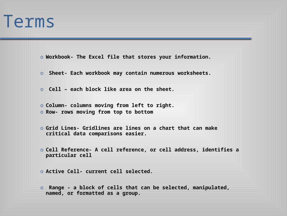
Terms

o Workbook- The Excel file that stores your information.

o Sheet- Each workbook may contain numerous worksheets.

o Cell – each block like area on the sheet.

o Column- columns moving from left to right.o Row- rows moving from top to bottom

o Grid Lines- Gridlines are lines on a chart that can make critical data comparisons easier.

o Cell Reference- A cell reference, or cell address, identifies a particular cell

o Active Cell- current cell selected.

o Range - a block of cells that can be selected, manipulated, named, or formatted as a group.

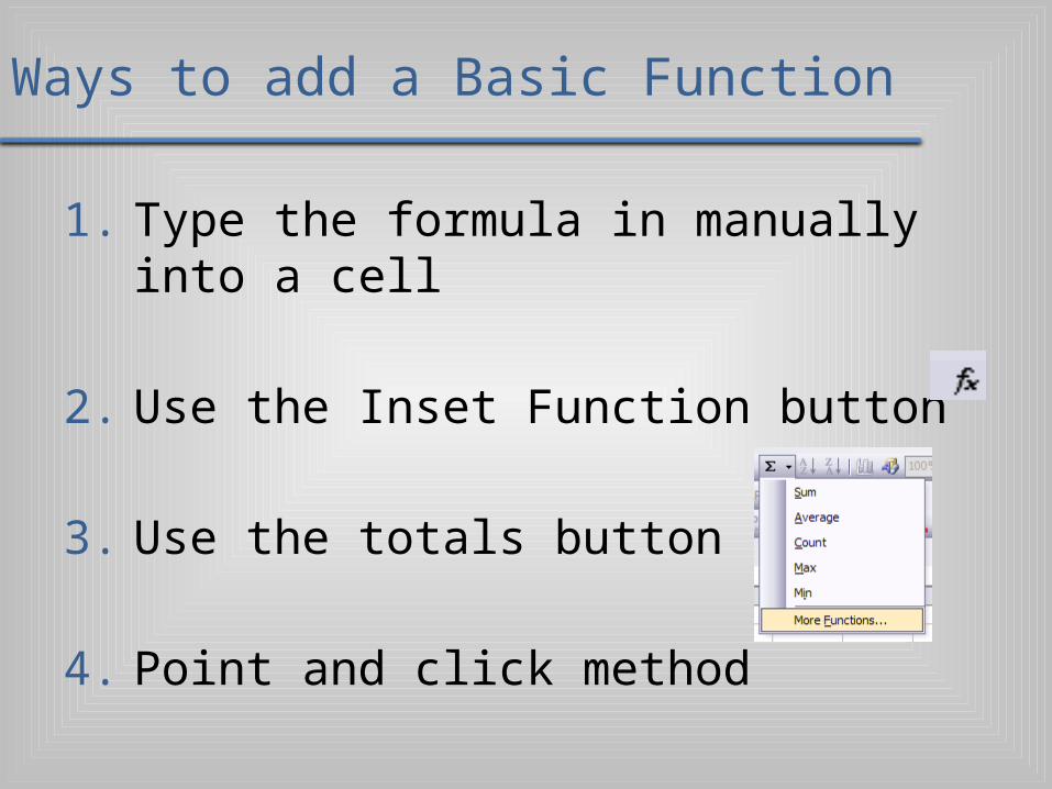
Ways to add a Basic Function

1. Type the formula in manually into a cell

2. Use the Inset Function button

3. Use the totals button

4. Point and click method

7

Plan Ahead

• Select titles and subtitles for the worksheet• Determine the contents for rows and columns• Determine the calculations that are needed• Determine where to save the workbook• Identify how to format various elements of the

worksheet• Decide on the type of chart needed• Establish where to position and how to format

the chart

Common Functions

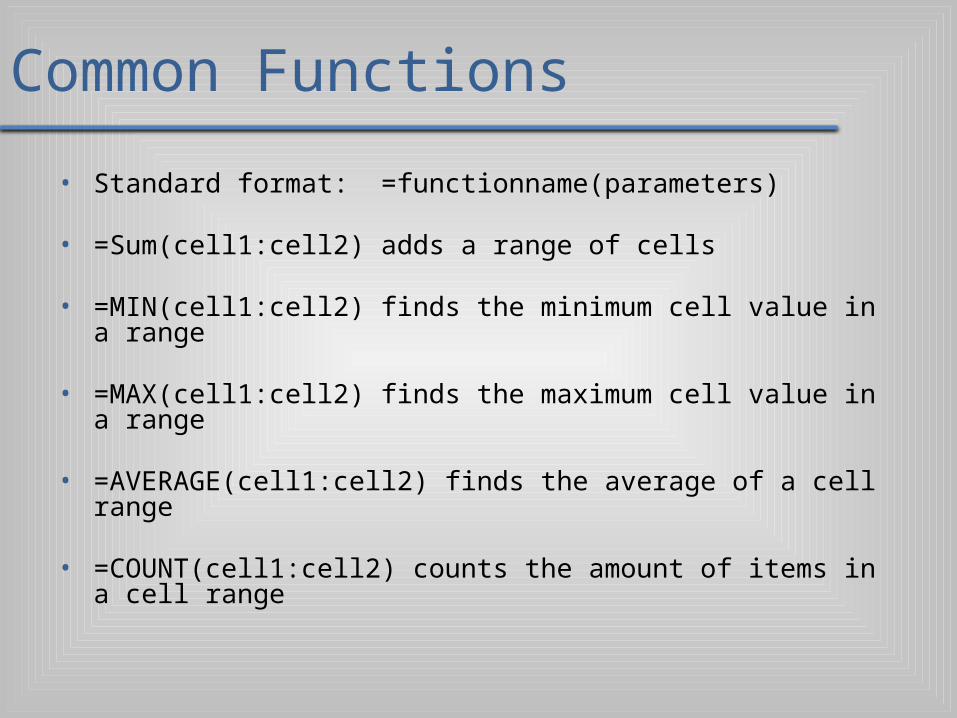
• Standard format: =functionname(parameters)

• =Sum(cell1:cell2) adds a range of cells

• =MIN(cell1:cell2) finds the minimum cell value in a range

• =MAX(cell1:cell2) finds the maximum cell value in a range

• =AVERAGE(cell1:cell2) finds the average of a cell range

• =COUNT(cell1:cell2) counts the amount of items in a cell range

9

Starting Excel

10

Entering the Worksheet Titles• Click cell A1 to make cell A1 the active cell• Type Walk and Rock Music in cell A1, and then

point to the Enter box in the formula bar• Click the Enter box to complete the entry and enter

the worksheet title in cell A1• Click cell A2 to select it• Type First Quarter Rock-It MP3 Sales

as the cell entry• Click the Enter box to complete the entry and enter

the worksheet subtitle in cell A2

11

Entering the Worksheet Titles

12

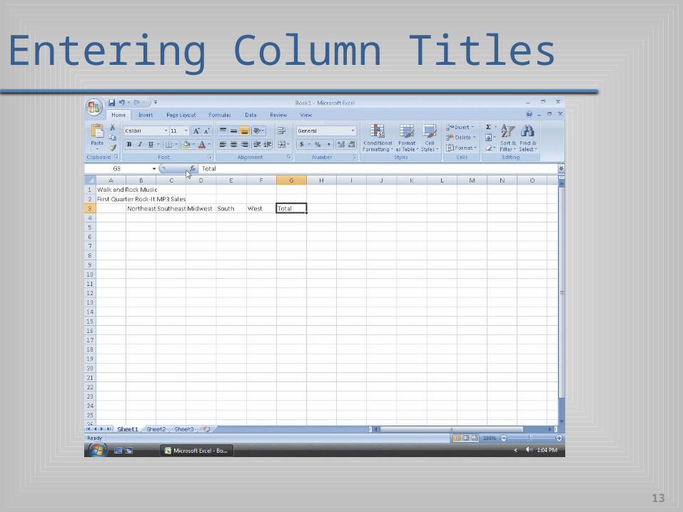
Entering Column Titles• Click cell B3 to make cell B3 the active cell• Type Northeast in cell B3• Press the RIGHT ARROW key to enter the column

title, Northeast, in cell B3 and make cell C3 the active cell

• Repeat Steps 2 and 3 to enter the remaining column titles in row 3; that is, enter Southeast in cell C3, Midwest in cell D3, South in cell E3, West in cell F3, and Total in cell G3 (complete the last entry in cell G3 by clicking the Enter box in the formula bar)

13

Entering Column Titles

14

Entering Row Titles

• Click cell A4 to select it• Type Video and then press the DOWN ARROW

key to enter the row title and make cell A5 the active cell

• Repeat Step 1 to enter the remaining row titles in column A; that is, enter Mini in cell A5, Micro in cell A6, Flash in cell A7, Accessories in cell A8, and Total in cell A9

15

Entering Row Titles

16

Entering Numbers• Click cell B4• Type 66145.15 and then press the RIGHT ARROW key

to enter the data in cell B4 and make cell C4 the active cell

• Enter 79677.1 in cell C4, 34657.66 in cell D4, 52517.2 in cell E4, and 99455.49 in cell F4

• Click cell B5• Enter the remaining first quarter sales numbers provided

in Table 1–1 on page EX 23 for each of the four remaining offerings in rows 5, 6, 7, and 8 to display the quarterly sales in the worksheet

17

Entering Numbers

18

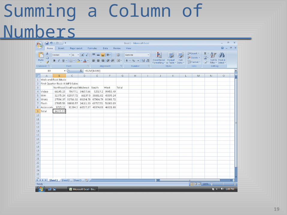
Summing a Column of Numbers• Click cell B9 to make it the active cell and then

point to the SUM button on the Ribbon• Click the Sum button on the Ribbon to display

=SUM(B4:B8) in the formula bar and in the active cell B9

• Click the Enter box in the formula bar to enter the sum of the first quarter sales for the five product types for the Northeast region in cell B9. Select cell B9 to display the SUM function assigned to cell B9 in the formula bar

19

Summing a Column of Numbers

20

Copying a Cell to Adjacent Cells in a Row

• With cell B9 active, point to the fill handle• Drag the fill handle to select the destination area,

range C9:F9, to display a shaded border around the destination area, range C9:F9, and the source area, cell B9. Do not release the mouse button

• Release the mouse button to copy the SUM function in cell B9 to the range C9:F9 and calculate the sums in cells C9, D9, E9, and F9

21

Copying a Cell to Adjacent Cells in a Row

22

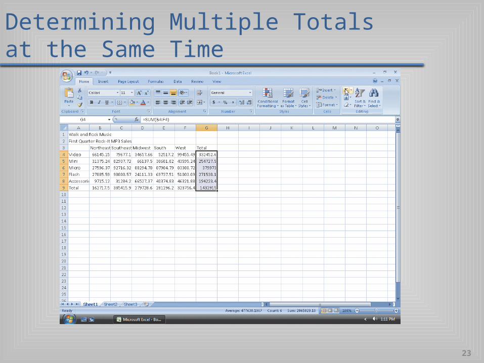
Determining Multiple Totals at the Same Time• Click cell G4 to make it the active cell• With the mouse pointer in cell G4 and in the

shape of a block plus sign, drag the mouse pointer down to cell G9 to highlight the range G4:G9 with a transparent view

• Click the Sum button on the Ribbon to calculate and display the sums of the corresponding rows of sales in cells G4, G5, G6, G7, G8, and G9

• Select cell A10 to deselect the range G4:G9

23

Determining Multiple Totals at the Same Time

24

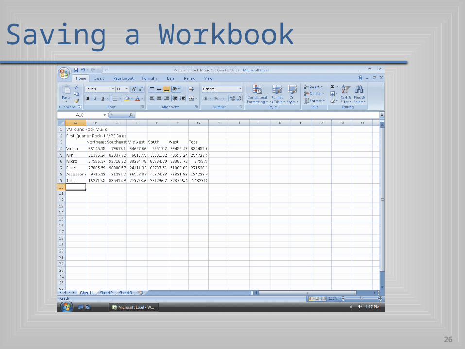
Saving a Workbook• With a USB flash drive connected to one of the computer’s USB ports,

click the Save button on the Quick Access Toolbar to display the Save As dialog box

• If the Navigation pane is not displayed in the Save As dialog box, click the Browse Folders button to expand the dialog box.

• If a Folders list is displayed below the Folders button, click the Folders button to remove the Folders list.

• Type Walk and Rock Music 1st Quarter Sales in the File name text box to change the file name. Do not press the ENTER key after typing the file name

• If Computer is not displayed in the Favorite Links section, drag the top or bottom edge of the Save As dialog box until Computer is displayed

• Click Computer in the Favorite Links section to display a list of available drives

25

Saving a Workbook

• If necessary, scroll until UDISK 2.0 (E :) appears in the list of available drives

• Double-click UDISK 2.0 (E:) in the Save in list to select the USB flash drive, Drive E in this case, as the new save location

• Click the Save button in the Save As dialog box to save the workbook on the USB flash drive with the file name, Walk and Rock Music 1st Quarter Sales

26

Saving a Workbook

27

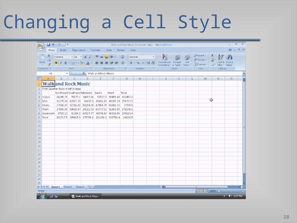
Changing a Cell Style

• Click cell A1 to make cell A1 the active cell• Click the Cell Styles button on the Ribbon to

display the Cell Styles gallery• Point to the Title cell style in the Titles and

Headings area of the Cell Styles gallery to see a live preview of the cell style in cell A1

• Click the Title cell style to apply the cell style to cell A1

28

Changing a Cell Style

29

Changing the Font Type

• Click cell A2 to make cell A2 the active cell• Click the Font box arrow on the Ribbon to display

the Font gallery• Point to Cambria in the Theme Fonts area of the

Font gallery to see a live preview of the Cambria font in cell A2

• Click Cambria in the Theme Fonts area to change the font type of the worksheet subtitle in cell A2 from Calibri to Cambria

30

Changing the Font Type

31

Bolding a Cell

• With cell A2 active, click the Bold button on the Ribbon to change the font style of the worksheet subtitle to bold

32

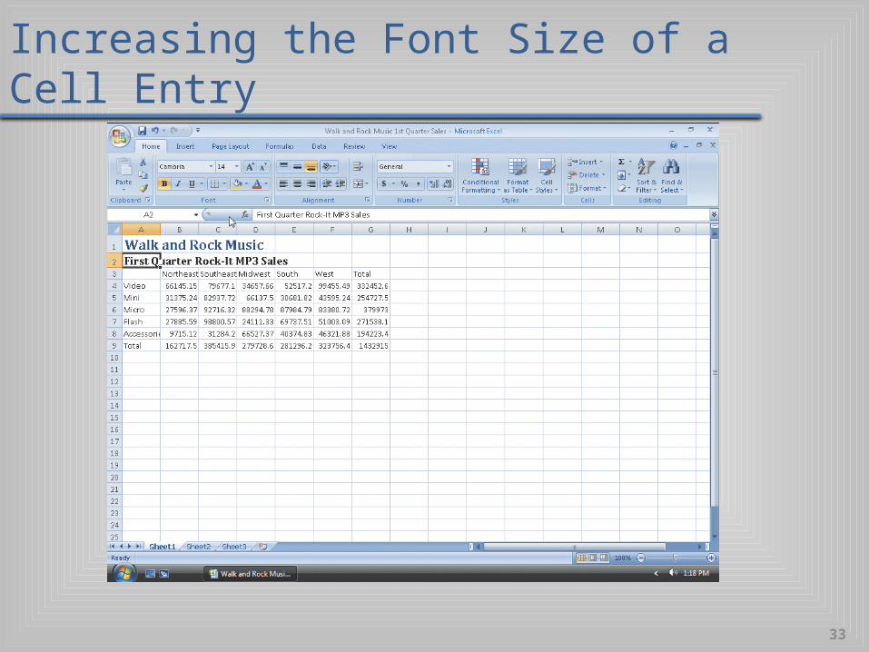
Increasing the Font Size of a Cell Entry

• With cell A2 selected, click the Font Size box arrow on the Ribbon to display the Font Size list

• Point to 14 in the Font Size list to see a live preview of cell A2 with a font size of 14

• Click 14 in the Font Size list to change the font in cell A2 from 11 point to 14 point

33

Increasing the Font Size of a Cell Entry

34

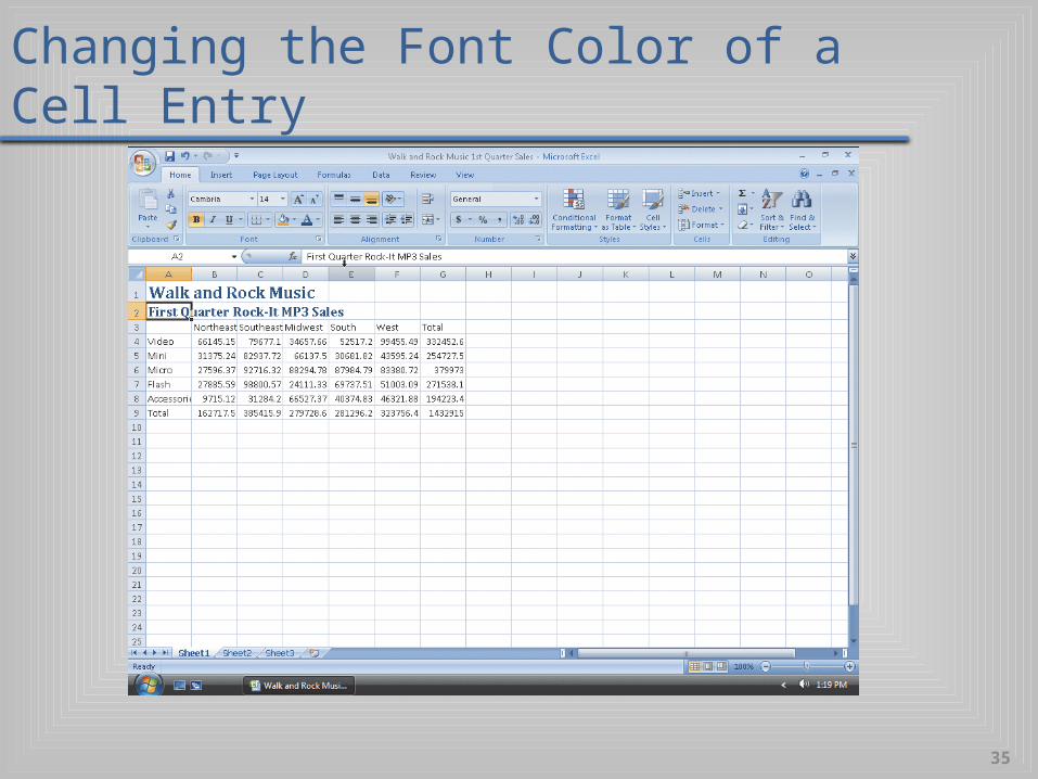
Changing the Font Color of a Cell Entry

• With cell A2 selected, click the Font Color button arrow on the Ribbon to display the Font Color palette

• Point to Dark Blue, Text 2 (dark blue color in column 4, row 1) in the Theme Colors area of the Font Color palette to see a live preview of the font color in cell A2

• Click Dark Blue, Text 2 (column 4, row 1) on the Font Color palette to change the font of the worksheet subtitle in cell A2 from black to dark blue

35

Changing the Font Color of a Cell Entry

36

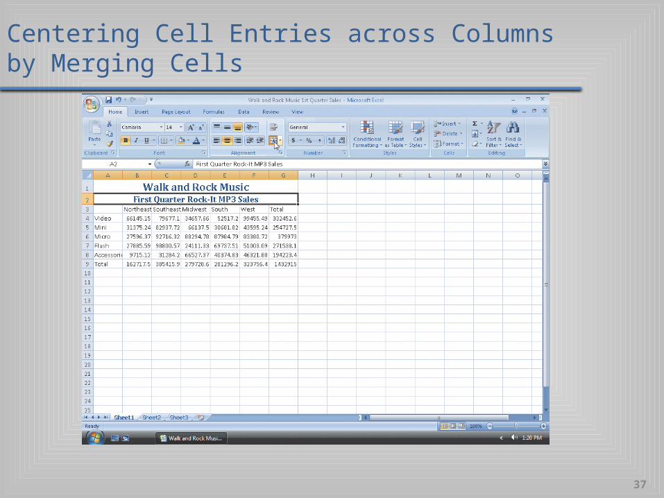
Centering Cell Entries across Columns by Merging Cells• Select cell A1 and then drag to cell G1 to

highlight the range A1:G1• Click the Merge and Center button on the Ribbon

to merge cells A1 through G1 and center the contents of cell A1 across columns A through G

• Repeat the first two steps to merge and center the worksheet subtitle across cells A2 through G2

37

Centering Cell Entries across Columns by Merging Cells

38

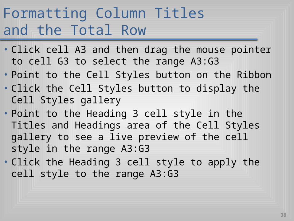
Formatting Column Titles and the Total Row• Click cell A3 and then drag the mouse pointer to cell

G3 to select the range A3:G3• Point to the Cell Styles button on the Ribbon• Click the Cell Styles button to display the Cell Styles

gallery• Point to the Heading 3 cell style in the Titles and

Headings area of the Cell Styles gallery to see a live preview of the cell style in the range A3:G3

• Click the Heading 3 cell style to apply the cell style to the range A3:G3

39

Formatting Column Titles and the Total Row• Click cell A9 and then drag the mouse pointer to

cell G9 to select the range A9:G9• Point to the Cell Styles button on the Ribbon• Click the Cell Styles button on the Ribbon to

display the Cell Styles gallery and then click the Total cell style in the Titles and Headings area to apply the Total cell style to the cells in the range A9:G9

• Click cell A11 to select the cell

40

Formatting Column Titles and the Total Row

41

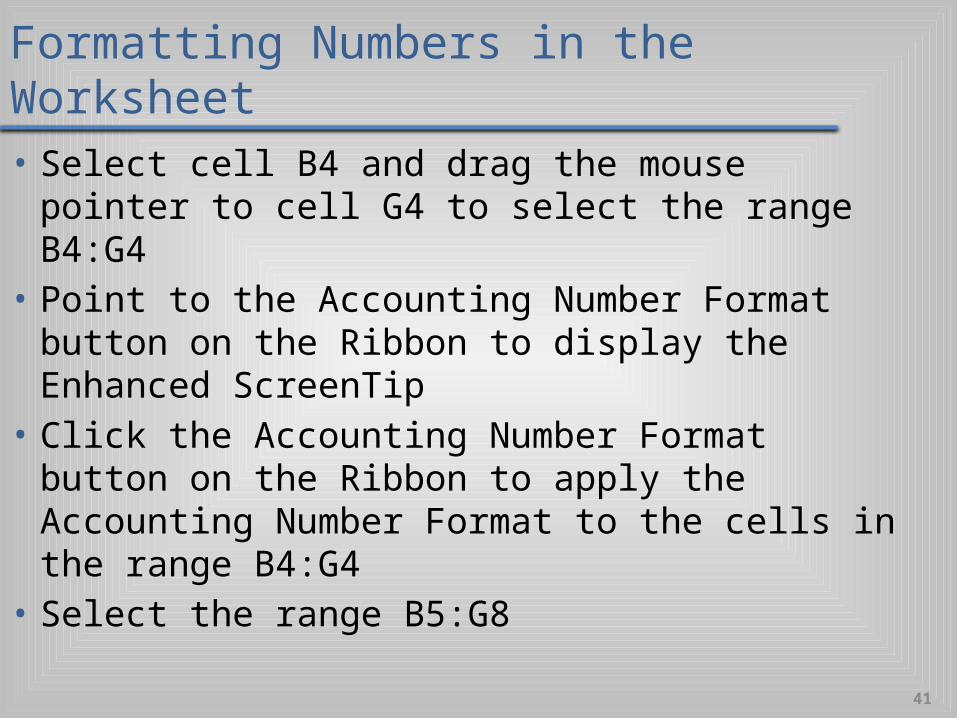
Formatting Numbers in the Worksheet

• Select cell B4 and drag the mouse pointer to cell G4 to select the range B4:G4

• Point to the Accounting Number Format button on the Ribbon to display the Enhanced ScreenTip

• Click the Accounting Number Format button on the Ribbon to apply the Accounting Number Format to the cells in the range B4:G4

• Select the range B5:G8

42

Formatting Numbers in the Worksheet

• Click the Comma Style button on the Ribbon to apply the Comma Style to the range B5:G8

• Select the range B9:G9• Click the Accounting Number Format button on

the Ribbon to apply the Accounting Number Format to the cells in the range B9:G9

• Select cell A11

43

Formatting Numbers in the Worksheet

44

Adjusting Column Width

• Point to the boundary on the right side of the column A heading above row 1 to change the mouse pointer to a split double arrow

• Double-click on the boundary to adjust the width of column A to the width of the largest item in the column

45

Adjusting Column Width

46

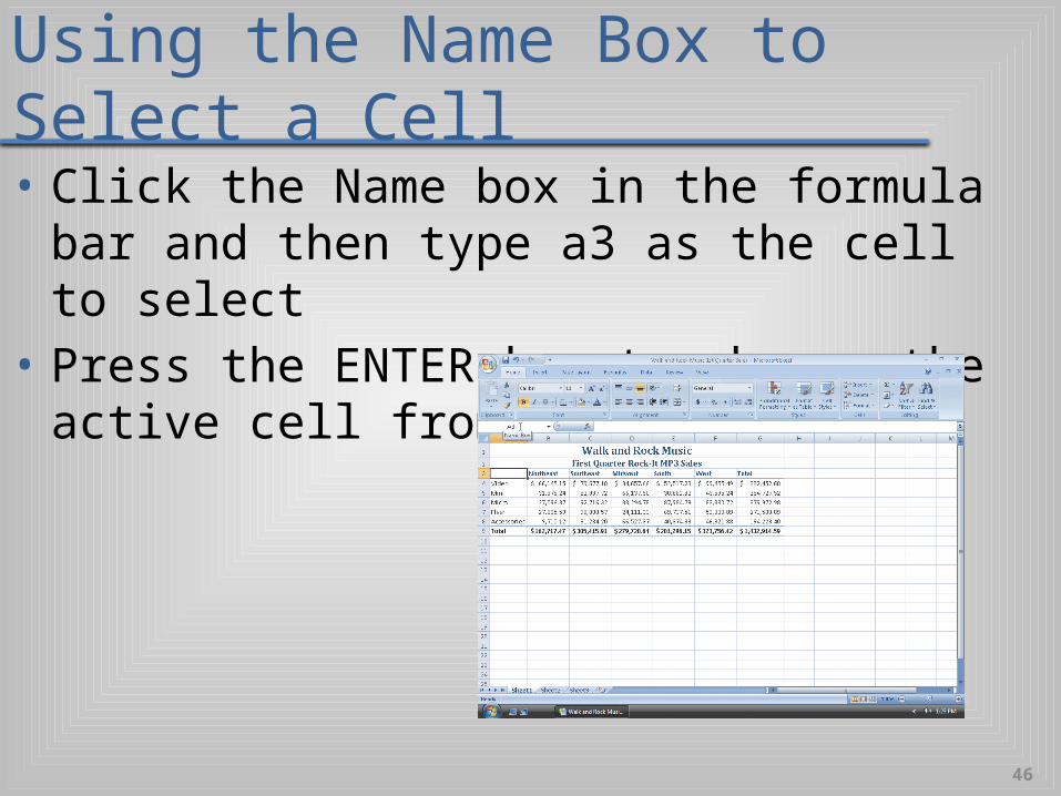
Using the Name Box to Select a Cell

• Click the Name box in the formula bar and then type a3 as the cell to select

• Press the ENTER key to change the active cell from A11 to cell A3

47

Adding a 3-D Clustered Column Chart to the Worksheet• Click cell A3 and then drag the mouse pointer to the cell

F8 to select the range A3:F8• Click the Insert tab to make the Insert tab the active tab• Click the Column button on the Ribbon to display the

Column gallery• Point to the 3-D Clustered Column chart type in the 3-D

Column area of the Column gallery• Click the 3-D Clustered Column chart type in the 3-D

Column area of the Column gallery to add a 3-D Clustered Column chart to the middle of the worksheet in a selection rectangle

48

Adding a 3-D Clustered Column Chart to the Worksheet• Click the top-right edge of the selection rectangle but do not release the

mouse to grab the chart and change the mouse pointer to a cross hair with four arrowheads

• Continue holding down the left mouse button while dragging the chart down and to the left to position the upper-left corner of the dotted line rectangle over the upper-left corner of cell A11. Release the mouse button to complete the move of the chart

• Click the middle sizing handle on the right edge of the chart and do not release the mouse button

• While continuing to hold down the mouse button, press the ALT key and drag the right edge of the chart to the right edge of column G and then release the mouse button to resize the chart

• Point to the middle sizing handle on the bottom edge of the selection rectangle and do not release the mouse button

49

Adding a 3-D Clustered Column Chart to the Worksheet• While continuing to hold down the mouse button, press

the ALT key and drag the bottom edge of the chart up to the bottom edge of row 22 and then release the mouse button to resize the chart

• Click the More button in the Chart Styles gallery to expand the gallery and point to Style 2 in the gallery (column 2, row 1)

• Click Style 2 in the Chart Styles gallery to apply the chart style Style 2 to the chart

• Click cell I9 to deselect the chart and complete the worksheet

50

Adding a 3-D Clustered Column Chart to the Worksheet

51

Changing Document Properties• Click the Office Button to display the Office Button menu• Point to Prepare on the Office Button menu to display the Prepare

submenu• Click Properties on the Prepare submenu to display the Document

Information Panel• Click the Author text box and then type your name as the Author

property. If a name already is displayed in the Author text box, delete it before typing your name

• Click the Subject text box, if necessary delete any existing text, and then type your course and section as the Subject property

• Click the Keywords text box, if necessary delete any existing text, and then type First Quarter Rock-It MP3 Sales

• Click the Close the Document Information Panel button so that the Document Information Panel no longer is displayed

52

Changing Document Properties

53

Saving an Existing Workbook with the Same File Name• With your USB flash

drive connected to one of the computer’s USB ports, click the Save button on the Quick Access Toolbar to overwrite the previous Walk and Rock Music 1st Quarter Sales file on the USB flash drive

54

Printing a Worksheet

• Click the Office Button to display the Office button menu

• Point to Print on the Office Button menu to display the Print submenu

• Click Quick Print on the Print submenu to print the document

55

Printing a Worksheet

56

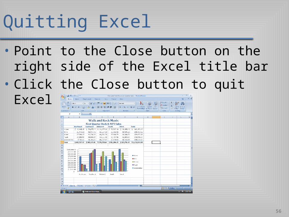
Quitting Excel

• Point to the Close button on the right side of the Excel title bar

• Click the Close button to quit Excel

57

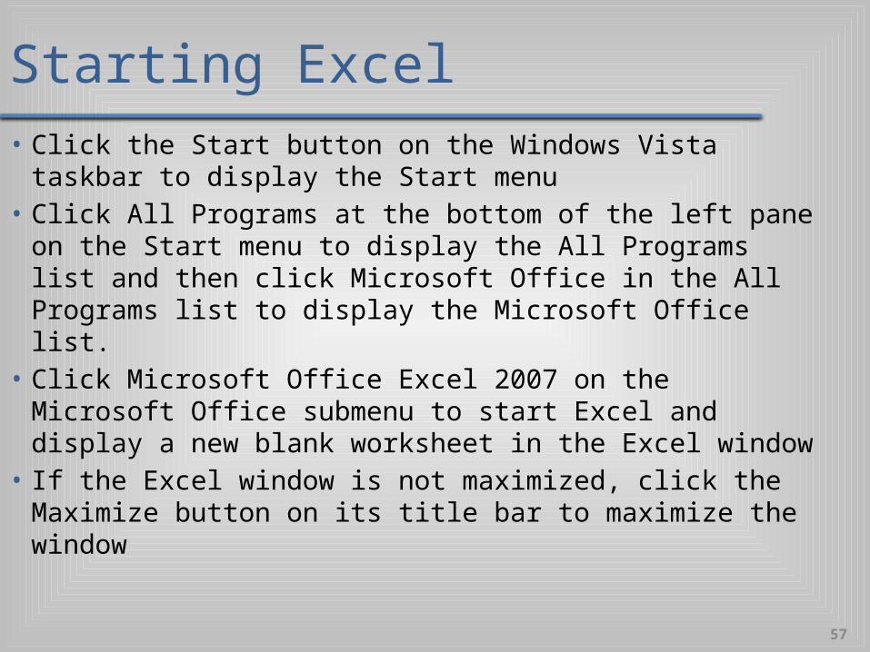
Starting Excel• Click the Start button on the Windows Vista taskbar to

display the Start menu• Click All Programs at the bottom of the left pane on the

Start menu to display the All Programs list and then click Microsoft Office in the All Programs list to display the Microsoft Office list.

• Click Microsoft Office Excel 2007 on the Microsoft Office submenu to start Excel and display a new blank worksheet in the Excel window

• If the Excel window is not maximized, click the Maximize button on its title bar to maximize the window

58

Opening a Workbook from Excel• With your USB flash drive connected to one of the computer’s USB

ports, click the Office Button to display the Office Button menu• Click Open on the Office Button menu to display the Open dialog box• If the Folders list is displayed below the Folders button, click the

Folders button to remove the Folders list• If necessary, click the Look in box arrow and then click UDISK 2.0 (E:) to

select the USB flash drive, Drive E in this case, in the Look in list as the new open location

• Double-click UDISK 2.0 (E:) to select the USB fl ash drive, Drive E in this case, as the new open location

• Click Walk and Rock Music 1st Quarter Sales to select the file name• Click the Open button to open the selected file and display the

worksheet in the Excel window

59

Opening a Workbook from Excel

60

Using the AutoCalculate Area to Determine a Maximum• Select the range B6:F6 and then right-click the

AutoCalculate area on the status bar to display the Status Bar Configuration shortcut menu

• Click Maximum on the shortcut menu to display the Maximum value in the range B6:F6 in the AutoCalculate area of the status bar

• Click anywhere on the worksheet to cause the shortcut menu to disappear

• Right-click the AutoCalculate area and then click Maximum on the shortcut menu to cause the Maximum value to no longer appear in the AutoCalculate area

61

Using the AutoCalculate Area to Determine a Maximum

62

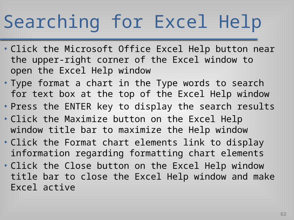
Searching for Excel Help• Click the Microsoft Office Excel Help button near the upper-

right corner of the Excel window to open the Excel Help window

• Type format a chart in the Type words to search for text box at the top of the Excel Help window

• Press the ENTER key to display the search results• Click the Maximize button on the Excel Help window title bar

to maximize the Help window• Click the Format chart elements link to display information

regarding formatting chart elements• Click the Close button on the Excel Help window title bar to

close the Excel Help window and make Excel active

63

Searching for Excel Help

64

Quitting Excel

• Click the Close button on the right side of the title bar to quit Excel

• If necessary, click the No button in the Microsoft Office Excel dialog box so that any changes you have made are not saved

65

Summary

• Start and quit Excel• Describe the Excel worksheet• Enter text and numbers• Use the Sum button to sum a range of cells• Copy the contents of a cell to a range of cells

using the fill handle

66

Summary

• Save a workbook• Format cells in a worksheet• Create a 3-D Clustered Column chart• Change document properties• Save a workbook a second time using the same

file name

67

Summary

• Print a worksheet• Open a workbook• Use the AutoCalculate area to determine

statistics• Correct errors on a worksheet• Use Excel Help to answer questions

Microsoft Office 2010

Excel Chapter 1 Complete