Microsoft Excel 2013 Consolidate Data & Analyze … · Microsoft Excel 2013 Consolidate Data &...

Copyright © 2005 ASCPL All Rights Reserved MS Excel Pivot Table 6/16/2015 MMS

1 of 20

Microsoft Excel 2013 Consolidate Data & Analyze with

Pivot Table

______________________________________________________________________________ Consolidate Data in Multiple Worksheets Example data is saved under Consolidation.xlsx workbook under ProductA through ProductD worksheets.

The consolidate function is used to summarize and report results from separate worksheets. You can consolidate data from each separate worksheet into a master worksheet. The worksheets can be in the same workbook as the master worksheet or in other workbooks. Your data in your worksheets do not have to be identical. However, the beauty of the Consolidate feature is that it can easily sum, count, average, etc. this data by looking at the labels. This is a lot easier than creating formulas.

For example, if you have a worksheet of monthly sales statements for each of your product lines, you might use a consolidation to roll up these figures into a corporate sales worksheet. This master worksheet might contain sales totals, various expense types, and total profit and expense figures for the entire enterprise.

To consolidate data, use the Consolidate command in the Data Tools group on the Data tab. Select 'sum' under Function box. Click on the red arrow in the Reference box to narrow the Consolidate window. Click on the first worksheet and select the range of cells you want to consolidate. Click on the red arrow to expand the Consolidate window. Click on the Add button. (You can name a range of cells and use those name ranges in the Reference box and click on the Add button.) Repeat this on all remaining worksheets you want to include in consolidation. See the example in Consolidation.xlsx workbook under Consolidate worksheet.

3-D Reference Cells: A 3-D reference is a useful and convenient way to reference several worksheets that follow the same pattern and cells on each worksheet and contain the same type of data, such as when you consolidate budget data from different departments in your organization. A reference that refers to the same cell or range on multiple sheets is called a 3-D reference. See example in Consolidation.xlsx workbook under 3DRefCell worksheet. Note:

If you insert or copy worksheets between two endpoints, then Excel includes all values in cells from the added worksheets in the calculations.

If you delete worksheets between two endpoints, then Excel removes their values from the calculation.

If you move worksheets from two endpoints to a location outside of the referenced worksheet range, then Excel removes their values from the calculation.

If you move either of two endpoints to another location in the same workbook, then Excel adjusts the calculation to include the new worksheets between them unless you reverse the order of the endpoints in the workbook. If you reverse the end points, the 3-D reference changes the endpoint worksheet. For example, say that you have a reference to


2 of 20

Sheet2:Sheet6: If you move Sheet2 after Sheet6 in the workbook, then the formula will point to Sheet3:Sheet6. If you move Sheet6 in front of Sheet2, the formula will adjust to point to Sheet2:Sheet5.

You can rename any worksheet and formula will adjust to the new names.

If you delete either two endpoints, then Excel removes the values on that worksheet from the calculation.

Subtotal Data

When you have a list of data in a column, you can automatically calculate subtotals and grand totals by using the Subtotal command in the Outline group on the Data tab. You may want to find out how much each of your customers is ordering in a particular quarter by using summary functions, such as Sum or Average in the SUBTOTAL. OR you can total the amount sold by each salesperson from an individual country, for example. You can display more than one type of summary function for each column. Remember to sort the list of data by your main criteria, then by any lower level criteria you wish to total. You can add a second level of subtotals by going through the same process and by selecting another sorted field and function. Just remember to uncheck the “Replace current subtotals” box to keep both levels of subtotals before clicking ‘OK’. Once you created the Subtotals, you will see the outline symbols at the upper left corner of the worksheet. See below. Click the largest number to display all data and summaries; click the smaller numbers to collapse the display and show summary data along. The number will get bigger as you add more nested subtotals.

See example in Consolidation.xlsx workbook under Subtotal1, Subtotal2, and Subtotal3 worksheets. To remove subtotals, click the Subtotals command again and click the “Remove All” button in the Subtotals box. Remove Duplicates The Remove Duplicates Function under the Data Tools group lets you remove duplicate values in a set of data. Click anywhere on the data that you are working on. Click the Remove Duplicates button under the Data tab. Check those boxes that you want to search for duplicates, and then click OK to remove the duplicate row. Remember the more number of boxes you check, the least number of duplicates will be removed and vice versa.

See example in Consolidation.xlsx workbook under RemoveDups worksheet.


3 of 20

Create a PivotTable Report

Creating a PivotTable report is about moving pieces of information around to see how they fit together. PivotTables reorganize, data, allowing you to look at your worksheet data in different ways. Pivoting data can help you answer different questions and even experiment with the data to discover new trends and patterns. Basically, PivotTable reports organize and summarize your data so that your excel data turns into information that makes sense. They offer comparisons, reveal patterns and relationships, and analyze trends. Use a PivotTable report when you want to make large, complex sets of data more comprehensible and easier to understand at a glance.

Before you open the PivotTable Wizard, ask yourself what you specifically need to know. Once you have your questions in mind, Excel makes it easy to get the answers. You decide what data you want analyzed, and how to organize it. Instead of a single arbitrary form that doesn't really suit your needs; each PivotTable report gives you a different view of your data, answering your questions on the spot, and is customized to your purposes.

You can answer different questions by arranging different Pivot Table reports. For example, take a look at the chart generated by a Pivot Table report below.

This chart could have been generated for various scenarios: Do you need to know sales totals by region, by salesperson, by quarter, or by month? Would your business do better if your best people sold only top products? Or would that mean whole product lines with no revenue?

Never worry about arranging a report in the "wrong" way. Creating a PivotTable report is about moving pieces of information around to see how they fit together. Move the data around, again and again, to get as many clear answers as you have questions. You may be using a different set of data to answer different questions.


4 of 20

The requirement of source data range for a pivot table

1. The source data range for a pivot table must be arranged in a list. To begin, you first need raw data to work with. The general rule is you need more than two criteria of data to work with—otherwise you have nothing to pivot.

2. Each record (observation) must be in a single row. 3. Each field (variable) must be in a single column. Note: Check that each column contains

only one sort of data—for example, include text in one column and numeric values in a separate column.

4. A header row must have names of the fields. 5. No blank rows or columns should be included in your data range (although blank cells within

the data are OK). 6. Remove any automatic subtotals. Don't worry; the PivotTable report will calculate the

subtotals and grand totals for you.

Assume you have data with sales figures that go on for many rows as shown in the example below. Download the practice workbook: SourceDataforSalespersons.xlsx to follow. (Source:

Microsoft.com)

How can you make the data more understandable? To find out, you would start by asking yourself what you need to know:

How much has each salesperson sold?

Who are the top 5?

What are the sales amounts by country? Now you have some idea from this huge data what you desire to find out. When you're ready to get the answers:

Click anywhere within the data or select all the data and columns you want to include in the report. (Note: If you click outside the data, you have to choose the data manually to analyze in your PivotTable report.)


5 of 20

On the Insert tab, click on Pivot Table under Tables group.

The Create PivotTable dialog box will appear.

Data range will be automatically selected. Select New Worksheet to place the PivotTable on a New Worksheet. Click OK.

Notice the PivotTable Tools bar appears on the top with two new tabs: Analyze and Design.

Next, the layout area appears in a new worksheet for the PivotTable report and also a list of the available fields on the PivotTable Field List. It takes less than a second to prepare a new worksheet that contains two items.

The layout area to drag items onto


6 of 20

The PivotTable Field List.

In the PivotTable, Field Lists are the names of the columns from the source data. In this example, they are: Country, Salesperson, Order Amount, Order Date, and OrderID.

Each column in the source data has become a field with the same name. To create a PivotTable report, you can either

1. Dragging fields from the field list and dropping them directly onto the bottom part of the Field List pane

2. By selecting the check box next to the field name

3. By right-clicking a field name and selecting a location to move the field to

Note: If you happen to click a cell outside of the report, the field list will disappear. To get it back, click inside the report again.

When you select a field by checking the box next to it, Excel places it in a default area of the layout for you. Fields that do not contain numbers go into the rows field on the left side of the report. Fields that contain numbers are placed into data fields on the right side of the report. You can move the field to another area if you want to. For example, if you want a field to be in the column area instead of the row area, you can do so easily.

For example, if you check the Salesperson field box or right-click on the field name and select Add to Row Labels, you would see one row for each salesperson's name in the left side of the PivotTable. If you prefer seeing the salesperson’s name in each column, you can right-click the field and select Add to Column Labels.

Remember that you don't have to use all the fields.


7 of 20

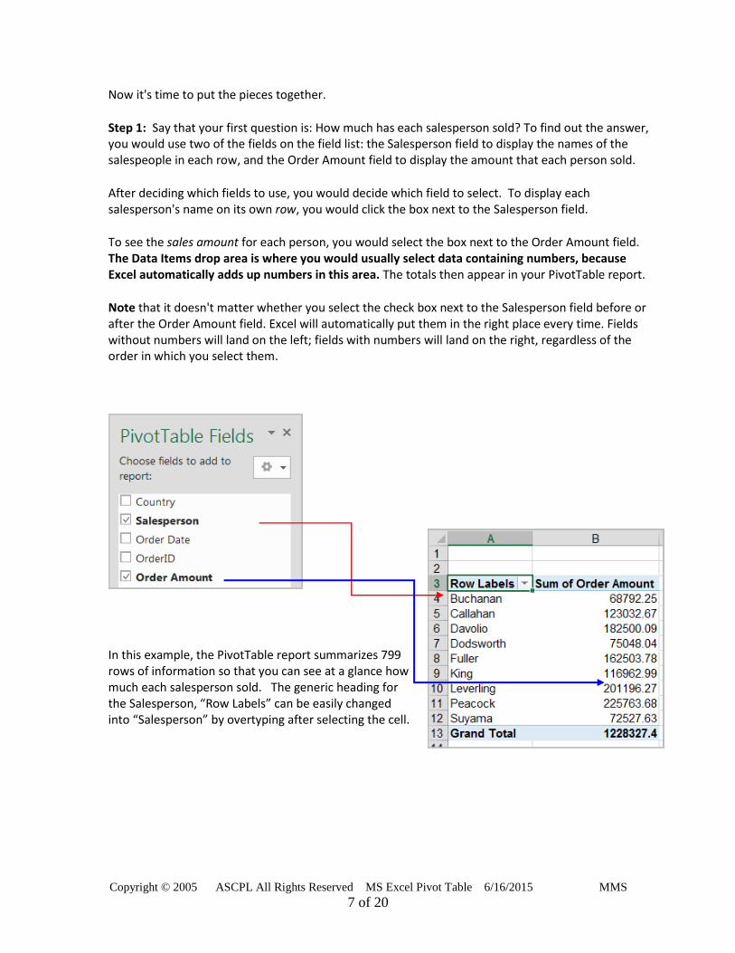
Now it's time to put the pieces together.

Step 1: Say that your first question is: How much has each salesperson sold? To find out the answer, you would use two of the fields on the field list: the Salesperson field to display the names of the salespeople in each row, and the Order Amount field to display the amount that each person sold.

After deciding which fields to use, you would decide which field to select. To display each salesperson's name on its own row, you would click the box next to the Salesperson field.

To see the sales amount for each person, you would select the box next to the Order Amount field. The Data Items drop area is where you would usually select data containing numbers, because Excel automatically adds up numbers in this area. The totals then appear in your PivotTable report.

Note that it doesn't matter whether you select the check box next to the Salesperson field before or after the Order Amount field. Excel will automatically put them in the right place every time. Fields without numbers will land on the left; fields with numbers will land on the right, regardless of the order in which you select them.

In this example, the PivotTable report summarizes 799 rows of information so that you can see at a glance how much each salesperson sold. The generic heading for the Salesperson, “Row Labels” can be easily changed into “Salesperson” by overtyping after selecting the cell.


8 of 20

Note: Downward-pointing arrows on field headings indicate that you can select how much detail to display in the report. For example, clicking the arrow on the Salesperson field reveals a list containing each salesperson's name; provides you with the ability to sort within the PivotTable report; or filter your data within the report.

To show only some of the names, click the box beside Show All to clear all the check marks. Then click beside each name you want to display, and then click OK. To display all the names again, click the arrow on the Salesperson field, click the box beside Show All, and then click OK.

Step 2: As you noticed, all salespeople are from two countries: UK and USA. If you would like to filter salespeople from one country at a time, right-click on Country field from your PivotTable Field List and select Add to Report Filter. Then, you can select from the drop-down arrow to display the country of your choice. See below. To see both countries, select All from your drop-down list again.

If you are compelled to see each country on a separate worksheet, click on the drop-down arrow next to the Options command under PivotTable group. Select Show Report Filter Pages and make selection of your filter, Country field. New worksheets with each filter name, USA and UK, in this example, will be automatically added.


9 of 20

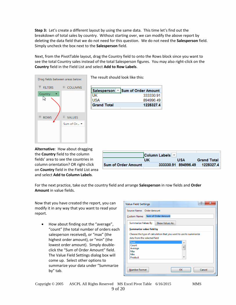
Step 3: Let’s create a different layout by using the same data. This time let’s find out the breakdown of total sales by country. Without starting over, we can modify the above report by deleting the data field that we do not need for this question. We do not need the Salesperson field. Simply uncheck the box next to the Salesperson field.

Next, from the PivotTable layout, drag the Country field to onto the Rows block since you want to see the total Country sales instead of the total Salesperson figures. You may also right-click on the Country field in the Field List and select Add to Row Labels.

The result should look like this:

Alternative: How about dragging the Country field to the column fields’ area to see the countries in column orientation? OR right-click on Country field in the Field List area and select Add to Column Labels. For the next practice, take out the country field and arrange Salesperson in row fields and Order Amount in value fields.

Now that you have created the report, you can modify it in any way that you want to read your report.

How about finding out the “average”, “count” (the total number of orders each salesperson received), or “max” (the highest order amount), or “min” (the lowest order amount). Simply double-click the “Sum of Order Amount” field. The Value Field Settings dialog box will come up. Select other options to summarize your data under “Summarize by” tab.


10 of 20

How about formatting Order Amount cells with US$ currency? While selecting the “Sum of Order Amount” cell (as shown above), click on the “Number Format” button. In the “Format Cells” window, select “Currency” under “Category” and select your decimal places option.

How about displaying the individual salesperson’s share of sales as a percentage of total sales? First, click on the “Number Format” button and bring out the “Format Cells” window, make sure to select “Percentage” in it. Click OK. Next, click on the “Show values as” tab in Value Field Settings dialog box and select “% of Parent Row total” from the drop-down box. See below.

The result should look like this:

To practice, keep the data back to Normal by using Currency and No Calculation under Show Values As in the Value Field Settings dialog box.


11 of 20

Let’s say you want to sort the salesperson column from top to bottom. Click on the drop-down box next to the “Salesperson” field. Click on “More Sort Options” to bring up the Sort dialog box. Select “Descending (Z to A) by: Sum of Order Amount”. Your data will be sorted by the largest amount of sales. See below.

Let’s say you want to find out the top 3 salespersons. Click on the drop-down box next to the “Salesperson” field. Under “Value Filters” click on “Top 10”. User the spinner to change the number to “3” to find top 3 salespersons. See below.

Indicates there is a

filter in this field!


12 of 20

Slicers

Slicers are basically just filters, allowing you to instantly pivot your data. If you frequently filter your PivotTables, consider using slicers since they're easier and faster to use. You can use these in place of filters.

To add a Slicer:

Select any cell in our already created PivotTable.

From the Analyze tab, click the Insert Slicer command.

A dialog box will appear. Select the desired field. In our example, we'll select Salesperson, then click OK.

The slicer will appear next to the table. Each selected item will be highlighted in blue as shown in the picture that all salesmen are selected.

Just like filters, only selected items are used in the PivotTable. When you select or deselect items, the PivotTable will instantly reflect the changes. Note: Press and hold the Ctrl key on your keyboard to select multiple non-adjacent items from a slicer. Use Shift key to select multiple adjacent items.

Use the Filter icon in the top-right corner to select all items from the slicer at once.


13 of 20

Inserting Timeline allows you to select time periods in order to filter.

Filer Connections will allow you to do multiple fields filtering such as Salesperson and Order Date together from your pivot data.

To delete the slicer, click on the border to select the entire slicer box then hit delete.

Border should look like this.

The PivotTable Tools Ribbon has other options:

If the Active Field displays show or hide details , you may click on the “+” sign and see the details of that particular field. Click on “-“sign to close the details.

Under Group, you may group or ungroup a range of cells. This command is suitable to group a time frame into smaller time frames, such as individual dates into months or quarters.

Under the Data group, you can click on Refresh to update your already created PivotTable report instantly when new data is inserted in the original source data. You can also change the outcome of your PivotTable report with a different data set by using Change Data Source.

Under the Actions group, you can click on Clear and select Clear All to start your PivotTable report from scratch. You can use Select to select an element of your PivotTable. Use Move PivotTable command to move the report to a new worksheet or into an existing worksheet in a different spot.

Under the Tools group, click on PivotChart to create a chart instantly on your PivotTable report. The PivotChart Filter Pane comes along with your chart so that you can modify your chart. Try using slicers or filters to change the data that is displayed. The PivotChart will automatically adjust to show the new data.

Use the Calculated Field command under Calculations Group to create and modify calculated fields or items.

o Assume you want to calculate a 15% commission to all salespersons and you wish to insert a new calculated field


14 of 20

called “Commission” added to your report. Here is how.

o Click the report.

o Under the Calculations group, click the drop-down arrow next to Fields, Items, … and then click Calculated Field. Insert Calculated Field box will appear.

o In the Name box, type a name “Commission” for the field.

o Use the Tab key on your keyboard to move to the Formula box. To use the data from another field in the formula, click the field in the Fields box (in this case, “Order Amount”), and then click Insert Field. Then Type in “*” (multiply) and “15%” to calculate a 15% commission on each value in the Sales field.

o Click Add, and then click OK. See below.

See your newly added Field in your PivotTable Field List.

Note: Use a calculated field when you want to use the data from another field in your formula. Use a calculated item when you want your formula to use data from one or more specific items (item: A subcategory of a field in the PivotTable and PivotChart reports. For instance, the field "Month" could have items such as "January," "February," and so on.) within a field.


15 of 20

Let’s say you want to change how a field name displays. Instead of “Sum of Order Amount”, you may change to your choice of name. Simply select the field, retype it and press enter. That’s simple!

What if you want to see the quarterly sales for each salesperson? As of now, the “Sum of Order Amount” is accumulated for the entire data across more than one year. We can add an “Order Date” field to the existing report. Simply click the check box next to the “Order Date” field and Excel will add it to below of each “Salesperson” field on the report. Now both the Order Date and Salesperson fields are in row orientation on the report, but the sales results are by day, followed by a total for the day. We need to “Group” the data into quarters for our purpose. Here is how.

Select any of a date cell and click on Group Selection or Group Field to bring up the Grouping dialog box. De-select “Months” and select “Years” and click OK. The result should show yearly figures for each salesperson.

Note: To ungroup data, simply click on the Ungroup command.

You can re-arrange fields by dragging fields (in the bottom right corner) to change the display. Drag the Order Date field above the Salesperson for practice. The display will change as shown on right.


16 of 20

A PivotTable report with more than one row field has one inner row field, the one closest to the data area. Any other row fields are outer row fields. Whether a row field is an inner or outer field determines how the data is displayed.

See the comparison below.

Salesperson is the outer field and Yr is the inner field.

Yr is the outer field and Salesperson is the inner field.

Why does that matter? An inner or outer row position determines how many times the items within the row field are repeated in the report, which is handy to know when you pivot on your own.

Items in the outermost row field are displayed only once.

Items in the rest of the row fields are repeated as necessary.

Details: You can easily list the records from the source data that are summarized in a particular data cell, just by double-clicking the cell. Excel creates a new worksheet like this one with a copy of the data. You can format, sort, and filter this detail data without affecting the PivotTable report or the original source data. For example, to find out which individual orders contributed to Buchanan's 2003 order amount, simply click the cell that has 2003 sales amount in it. A new sheet will appear with all 2003 data belonged to Buchanan.

You can change the format of your PivotTable report. Normally you would leave the formatting until you’re through pivoting the report. Click on the Design tab under the PivotTable Tools ribbon and select the design you like. Use the scroll bar to view more designs.

Double-clicking

here will show

the details of this

figure!


17 of 20

Consolidating Multiple Data Worksheets in your PivotTable Report (Source: Microsoft.com) Let’s add the PivotTable and PivotChart Wizard to the Quick Access Toolbar before we perform consolidation of multiple data worksheets.

1. Click the arrow next to the Quick Access Toolbar and then click More Commands.

2. Under Choose commands from, select All Commands.

3. In the list, select PivotTable and PivotChart Wizard, click Add, and then click OK.

Setting up the source data

You can summarize and report results from separate worksheet ranges from the same workbook or in a different workbook. Each range of data should be in cross-tab format, with matching row and column names for items that you want to summarize together. The source worksheets do not even have to be identical, just similar. Data should have column labels in the first row, row labels in the first column, the rest of the rows having similar items in the same row and column, and no blank rows or columns within the range. Do not include any total rows or total columns from the source data when you specify the data for the report.

Using named ranges

To make the report easier to update, name (name: A word or string of characters that represents a cell, range of cells, formula, or constant value. Use easy-to-understand names, such as Products, to refer to hard to understand ranges, such as Sales!C20:C30.) each source range and use the names when you create the PivotTable or PivotChart report. If a source range expands, you can update the range for the name in the separate worksheet to include the new data before you refresh the PivotTable report.

Open Multiple Consolation Examples.xlsx workbook. In this workbook, the data ranges (A3xM10) are already named as Product_A, Product_B, Product_C respectively to include in our consolidation. The title cell from row 2 on each worksheet is left out on purpose.

Page fields in consolidations

You can consolidate data by using a single page field or multiple page fields.

Single page field: If you're consolidating budget data from the Marketing, Sales, and Manufacturing departments, a page field could include one item to display the data for each department plus an item to show the combined data. To include one page field with an item for each source range plus an item that consolidates all of the ranges:

1. Click a blank cell in the workbook that is not part of a PivotTable report.


18 of 20

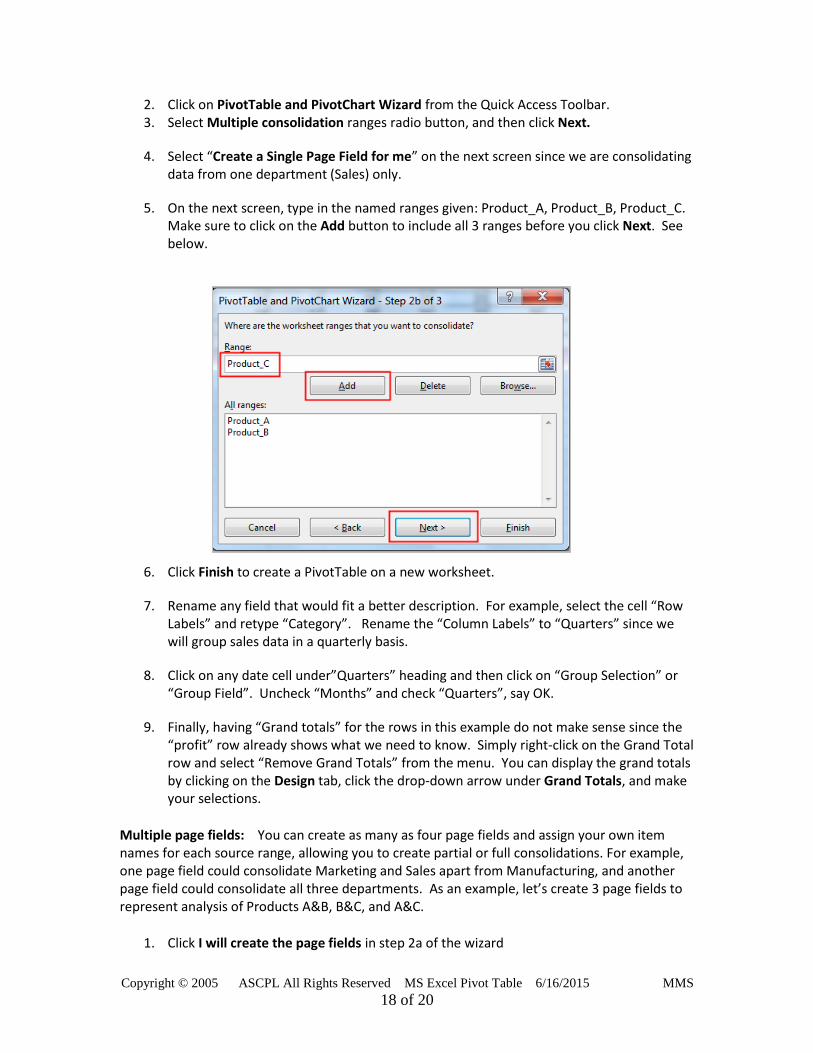
2. Click on PivotTable and PivotChart Wizard from the Quick Access Toolbar. 3. Select Multiple consolidation ranges radio button, and then click Next.

4. Select “Create a Single Page Field for me” on the next screen since we are consolidating data from one department (Sales) only.

5. On the next screen, type in the named ranges given: Product_A, Product_B, Product_C. Make sure to click on the Add button to include all 3 ranges before you click Next. See below.

6. Click Finish to create a PivotTable on a new worksheet.

7. Rename any field that would fit a better description. For example, select the cell “Row Labels” and retype “Category”. Rename the “Column Labels” to “Quarters” since we will group sales data in a quarterly basis.

8. Click on any date cell under”Quarters” heading and then click on “Group Selection” or “Group Field”. Uncheck “Months” and check “Quarters”, say OK.

9. Finally, having “Grand totals” for the rows in this example do not make sense since the “profit” row already shows what we need to know. Simply right-click on the Grand Total row and select “Remove Grand Totals” from the menu. You can display the grand totals by clicking on the Design tab, click the drop-down arrow under Grand Totals, and make your selections.

Multiple page fields: You can create as many as four page fields and assign your own item names for each source range, allowing you to create partial or full consolidations. For example, one page field could consolidate Marketing and Sales apart from Manufacturing, and another page field could consolidate all three departments. As an example, let’s create 3 page fields to represent analysis of Products A&B, B&C, and A&C.

1. Click I will create the page fields in step 2a of the wizard


19 of 20

2. In step 2b, select the cell range on the worksheet to include each cell range. Include all cell ranges for Products A, B, & C. Select the cell range for each page field or type in range names and click on Add.

3. Under How many page fields do you want? , click the number of page fields that you want to use. In this example, select the radio button for 3: A&B, B&C and A&C.

4. Under What item labels do you want each page field to use to identify the selected data range?, do the following:

1) Click on Product_A in All ranges box. Type in A&B in Field one box.

2) Click on Product_B in All ranges box. Select A&B in Field one box by using the

drop-down box.

3) You are still selecting Product_B in All ranges box at this time. In Field two box,

type in B&C.

4) Click on Product_C in All ranges box. Select B&C in Field two box by using the

drop-down box.

5) You are still selecting Product_C in All ranges box at this time. In Field three

box, type in A&C.

6) Click on Product_A in All ranges box. Select A&C in Field three box by using the

drop-down box.

7) Click on Next button on the bottom.

8) Select New Worksheet button to place the PivotTable on the new worksheet.

Each Page Filter Field above should come with blank field. Blank field assures that on each filter that a field is excluded from this filter. For example, in Filter A&B, if you click on blank field, the result shows the data from Product_C which is exactly what you excluded when you built Filter

A&B.

Turn on the Filter pages, Page1, Page2, and Page3 one at a time and make sure to select A&B from Page1; B&C from Page2, and A&C from Page3 to see the results.

Note: You can simply select the cell “Page1” and rename “Product A&B” by over-typing on it. Do the same for “Page2” to rename “Product B&C” and “Page3” to rename “Product A&C”. Also, when you turn on each filter in PivotTable Field List: Page1 or Page2 or Page3, right-click on them and select Add to Report Filter.


20 of 20

Sources

http://office.microsoft.com/training/:

PivotTable I: What's so great about PivotTable reports?

PivotTable II: Swing into action with PivotTable reports

PivotTable III: Show off your PivotTable skills

http://office.microsoft.com/en-us/excel/HA010346331033.aspx

Check out 3 other great PivotTable reports on Microsoft website. You can get them here by clicking on the links below:

1. Compare Your Customers

2. Compare Your Products

3. Compare Your Orders

John F. Lacher & Associates, LLC.

PivotTable Multiple Consolidation Example

http://office.microsoft.com/training/

http://office.microsoft.com/training/training.aspx?AssetID=RC010136191033

http://office.microsoft.com/search/redir.aspx?AssetID=RC010286901033&CTT=5&Origin=RP010140321033

http://office.microsoft.com/search/redir.aspx?AssetID=RC010381561033&CTT=5&Origin=RP010140321033

http://office.microsoft.com/en-us/excel/HA010346331033.aspx

http://www.akronlibrary.org/training/pdf/SampleCustomerReports.xls

http://www.akronlibrary.org/training/pdf/SampleProductReports.xls

http://www.akronlibrary.org/training/pdf/SampleOrderReports.xls

http://www.lacher.com/

http://www.lacher.com/examples/lacher05.htm

Microsoft Excel 2013 Consolidate Data & Analyze … · Microsoft Excel 2013 Consolidate Data &...

Documents

Transcript of Microsoft Excel 2013 Consolidate Data & Analyze … · Microsoft Excel 2013 Consolidate Data &...