Microsoft Excel 2010 Intermediate Excel.… · Microsoft Excel 2010 Intermediate Microsoft Excel is...

Training & Technology Solutions

Queens College ~ Office of Information Technology ~ Training & Technology Solutions

718-997-4875 ~ [email protected] ~ I-Bldg 214

Microsoft Excel 2010 Intermediate

Microsoft Excel is the most popular spreadsheet program used in businesses and organizations

today. A spreadsheet contains a grid of rows and columns that can enable users to organize data

and recalculate results for cells containing formulas when any data in the cells is changed.

Columns

The columns are labeled on top with letters and they go from top to bottom.

Rows

The rows are labeled on the left with numbers and they go from left to right.

Cells

Cells are the individual boxes in Excel. For example, if you click on the first box, it

would be called Cell A1.

Rows are labeled with numbers.

Columns are labeled with letters.

mailto:[email protected]




Type up the Following Example:

To Perform Mathematical Calculations:

When entering a mathematical formula into the formula box, you must precede it with an equal

sign. Use the following to indicate the type of calculation you wish to perform:

Note: Formulas can be as simple or as complex as necessary but you must remember that they

always begin with an = sign and contain mathematical operations.





Calculating the SUM, AVERAGE, MIN, and MAX

SUM

A) Now if we wanted to calculate the totals for the month of April, we would have to do the

following:

Click on cell C12 and type an = sign.

Click on cell C4 and type a + sign.



Click on cell C10 and press Enter (or Return)

This should populate the totals for the month of April in cell C12. You can use this procedure fill

out the rest of the months as well.

B) Another way to find the sum each individual month would be to:

Click on C12 and type in “ =SUM(B4:B10) “

This can be repeated for every other month as well.

C) Another option would be to highlight all of the amounts for one month, including the empty

cell for the totals:

And then clicking on the AutoSum button under the Formula tab. This will sum up all the

highlighted cells and populate the total in the last cell that was highlighted.





AVERAGE

You can use the methods to find the SUM, to find the AVERAGE as well. Just substitute the

word SUM with AVERAGE wherever needed.

Finding the Lowest and Highest Numbers

MIN

You can use the MIN function to find the lowest number in a series of numbers. To find the MIN

you should:

Click on an empty cell underneath the month you are finding the MIN for.

Type “=MIN(B4:B10)” or click on the empty cell, use the dropdown for AutoSum to pick MIN

and then highlight the cells that you want used in your formula.

MAX

You can use the MAX function to find the highest number in a series of numbers. To find the

MAX you should:

Click on an empty cell underneath the month you are finding the MAX for.

Type “ =MAX(B4:B10)” or click on the empty cell, use the dropdown for AutoSum to pick

MAX and then highlight the cells that you want used in your formula.





Creating a Header and Footer

1. Click on the Insert Tab and choose the Header and Footer button.

Note: the Page Layout will change and a Design tab will appear on top.

2. Click the left side of the Header area and type in your name. When you go to print this document,

Excel will place your name in the upper left corner.

3. Click the Go to Footer button and Excel will move to the Footer area. Here you can type in “Your

Department Name” and “Your email address”.

4. To return to the normal view again, choose the View tab and click on the Normal button.





Creating Charts

In Excel, you can represent numbers in a chart. On the Insert tab, there are a variety of charts to

choose from, including column, line, pie, bar, area, and scatter.

The basic procedure for creating a chart is the same no matter what type of chart you choose. As

you change your data, the chart will automatically update.

Creating a Column Chart

1. You must select all the cells containing the data you want in the chart. In this case, select cells A3

to F10.





2. Choose the Insert tab and click on the Column button in the Charts group.

3. Click on the Clustered Column chart subtype. (The first 2-D column option). The chart will

appear on your Excel sheet.





Applying a Chart Layout

1. Click on the chart in your Excel worksheet and the Design tab becomes available again.

2. Move to the Chart Layout group and click on Layout 5.





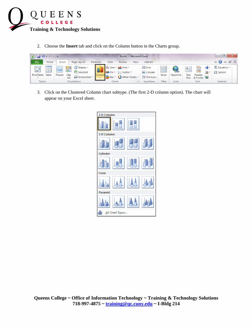
The chart will change from:

To Change the Chart Title and the Axis Title, just click on either title box, delete what is already

written in there, and type in the new titles.

In this case, Chart Title will be changed to Yearly Budget and the Axis Title will be changed to

Spending.





Switching Data

If you wish to change what displays in your chart, you can switch from row data to column data.

To do so:

1. Click on the Design tab.

2. Click the Switch Row/ Column button.

Your chart will now look like this:





Filtering and Deleting Duplicate Records

If you have a chart that has a lot of data, you may want to check to see if there are any cells that

hold unnecessary duplicate information. You can delete these duplicates to make your chart

clean and more precise.

In this example, there are four rows that have the same exact data.

1. Select all of the rows that you want to filter, including the headers, by selecting all the

cells containing the data you want in the chart. In this case, select cells A2 to F9.





2. In the Data tab, click on Advanced Filter.

Make sure that the Unique records only box is checked off. Then, click OK.

3. The duplicate rows will be removed from the chart.





Sorting Data

Sorting data may be helpful if you need to organize your data in alphabetical order. This

can also be used as an alternate way to identify duplicate rows in your data.

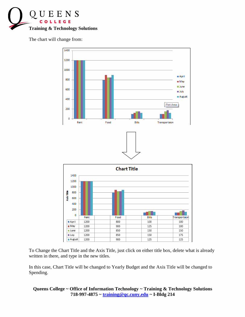
1. Select all of the rows that you want to sort, including the headers, by selecting all the cells

containing the data you want in the chart. In this case, select cells A2 to F9.

2. In the Data tab, click on Sort.





3. In the Sort window, click on the Sort by drop down box and select which column you want to

sort from. For this example, we are going to sort by the “Items” column. Once you have chosen

which column you are going to be sorting by, click on OK.

4. Your chart will now be sorted.


Microsoft Excel 2010 Intermediate Excel.… · Microsoft Excel 2010 Intermediate Microsoft Excel is...

Documents

Transcript of Microsoft Excel 2010 Intermediate Excel.… · Microsoft Excel 2010 Intermediate Microsoft Excel is...