MicroscaleHeatTransfer - The Library of...
50
BOOKCOMP, Inc. — John Wiley & Sons / Page 1309 / 1st Proofs / Heat Transfer Handbook / Bejan 1 2 3 4 5 6 7 8 9 10 11 12 13 14 15 16 17 18 19 20 21 22 23 24 25 26 27 28 29 30 31 32 33 34 35 36 37 38 39 40 41 42 43 44 45 [First Page] [1309], (1) Lines: 0 to 86 ——— * 17.67409pt PgVar ——— Normal Page * PgEnds: PageBreak [1309], (1) CHAPTER 18 Microscale Heat Transfer ANDREW N. SMITH Department of Mechanical Engineering United States Naval Academy Annapolis, Maryland PAMELA M. NORRIS Department of Mechanical and Aerospace Engineering University of Virginia Charlottesville, Virginia 18.1 Introduction 18.2 Microscopic description of solids 18.2.1 Crystalline structure 18.2.2 Energy carriers 18.2.3 Free electron gas 18.2.4 Vibrational modes of a crystal 18.2.5 Heat capacity Electron heat capacity Phonon heat capacity 18.2.6 Thermal conductivity Electron thermal conductivity in metals Lattice thermal conductivity 18.3 Modeling 18.3.1 Continuum models 18.3.2 Boltzmann transport equation Phonons Electrons 18.3.3 Molecular approach 18.4 Observation 18.4.1 Scanning thermal microscopy 18.4.2 3ω technique 18.4.3 Transient thermoreflectance technique 18.5 Applications 18.5.1 Microelectronics applications 18.5.2 Multilayer thin-film structures 18.6 Conclusions Nomenclature References 1309
Transcript of MicroscaleHeatTransfer - The Library of...
BOOKCOMP, Inc. — John Wiley & Sons / Page 1309 / 1st Proofs / Heat Transfer Handbook / Bejan
123456789101112131415161718192021222324252627282930313233343536373839404142434445
[First Page]
[1309], (1)
Lines: 0 to 86
———* 17.67409pt PgVar
———Normal Page
* PgEnds: PageBreak
[1309], (1)
CHAPTER 18
Microscale HeatTransfer
ANDREW N. SMITH
Department of Mechanical EngineeringUnited States Naval AcademyAnnapolis, Maryland
PAMELA M. NORRIS
Department of Mechanical and Aerospace EngineeringUniversity of VirginiaCharlottesville, Virginia
18.1 Introduction
18.2 Microscopic description of solids18.2.1 Crystalline structure18.2.2 Energy carriers18.2.3 Free electron gas18.2.4 Vibrational modes of a crystal18.2.5 Heat capacity
Electron heat capacityPhonon heat capacity
18.2.6 Thermal conductivityElectron thermal conductivity in metalsLattice thermal conductivity
18.3 Modeling18.3.1 Continuum models18.3.2 Boltzmann transport equation
PhononsElectrons
18.3.3 Molecular approach
18.4 Observation18.4.1 Scanning thermal microscopy18.4.2 3ω technique18.4.3 Transient thermoreflectance technique
18.5 Applications18.5.1 Microelectronics applications18.5.2 Multilayer thin-film structures
18.6 Conclusions
Nomenclature
References
1309

BOOKCOMP, Inc. — John Wiley & Sons / Page 1310 / 1st Proofs / Heat Transfer Handbook / Bejan
1310 MICROSCALE HEAT TRANSFER
123456789101112131415161718192021222324252627282930313233343536373839404142434445
[1310], (2)
Lines: 86 to 109
———0.0pt PgVar———Short Page
PgEnds: TEX
[1310], (2)
18.1 INTRODUCTION
The microelectronics industry has been driving home the idea of miniaturization forthe past several decades. Smaller devices equate to faster operational speeds and moretransportable and compact systems. This trend toward miniaturization has an infec-tious quality, and advances in nanotechnology and thin-film processing have spread toa wide range of technological areas. A few examples of areas that have been affectedsignificantly by these technological advances include diode lasers, photovoltaic cells,thermoelectric materials, and microelectromechanical systems (MEMSs). Improve-ments in the design of these devices have come mainly through experimentation andmacroscale measurements of quantities such as overall device performance. Moststudies of the microscale properties of these devices and materials have focused oneither electrical and/or microstructural properties. Numerous thermal issues, whichhave been largely overlooked, currently limit the performance of modern devices.Hence the thermal properties of these materials and devices are of critical importancefor the continued development of high-tech systems.
The need for increased understanding of the energy transport mechanisms ofthin films has given rise to a new field of study called microscale heat transfer.Microscale heat transfer is simply the study of thermal energy transfer when theindividual carriers must be considered or when the continuum model breaks down.The continuum model for heat transfer has classically been the conservation of energycoupled with Fourier’s law for thermal conduction. In an analogous manner, thestudy of “gas dynamics” arose when the continuum fluid mechanics models wereinsufficient to explain certain phenomena. The field of microscale heat transfer bearssome striking similarities. One area of similarity is in the methodology. Usually, thefirst attempt at modeling is to modify the continuum model in such a way that themicroscale considerations are taken into account. The more common and slightlymore difficult method is application of the Boltzmann transport equation. Finally,when both of these methods fail, the computationally exhaustive molecular dynamicsapproach is typically adopted. These three methods and specific applications will bediscussed in more detail.
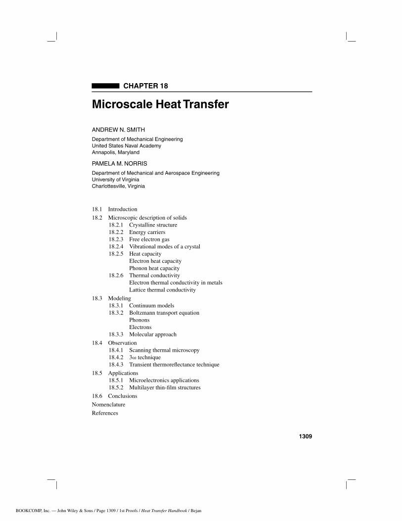
Figure 18.1 demonstrates four different mechanisms by which electrons, the pri-mary heat carriers in metallic films, can be scattered. All of these scattering mecha-nisms are important in the study of microscale heat transfer. The mean free path of anelectron in a bulk metal is typically on the order of 10 to 30 nm, where electron latticescattering is dominant. However, when the film thickness is on the order of the meanfree path, boundary scattering comes important. This is referred to as a size effectbecause the physical size of the film influences the transport properties. Thin filmsare manufactured using a number of methods and under a wide variety of conditions.This can have a serious influence on the microstructure of the film, which influencesdefect and grain boundary scattering. Finally, when heated by ultrashort pulses, theelectron system becomes so hot that electron–electron scattering can become signifi-cant. Thus, microscale heat transfer requires consideration of the microscopic energycarriers and the full range of possible scattering mechanisms.
BOOKCOMP, Inc. — John Wiley & Sons / Page 1311 / 1st Proofs / Heat Transfer Handbook / Bejan
INTRODUCTION 1311
123456789101112131415161718192021222324252627282930313233343536373839404142434445
[1311], (3)
Lines: 109 to 113
———-2.903pt PgVar———Short Page
PgEnds: TEX
[1311], (3)
Figure 18.1 Primary scattering mechanisms of free electrons within a metal.
In the first section of this chapter we focus on defining and describing the mi-croscopic heat carriers. The free electrons are typically responsible for thermal trans-port in metals. The governing statistical distribution is presented and discussed, alongwith equations for thermal conduction and the electron heat capacity. In an insulatingmaterial, thermal transport is accomplished through the motion of lattice vibrationscalled phonons. These lattice vibrations or phonons are discussed in detail. The pri-mary heat carriers in semiconductor materials are also phonons, and therefore thethermal transport properties of semiconductors are determined in the same manneras for insulating materials. The formulations for these energy carriers are then usedto explain and calculate the phonon thermal conductivity and lattice heat capacity ofcrystalline materials.
Experimental observation and measurement of microscale thermophysical prop-erties is the subject of the next section. These techniques can be either steady-state,modulated, or pulsed transient techniques. Steady-state techniques typically focus onmeasuring the surface temperature with high spatial resolution, while the transienttechniques are better suited for measuring transport properties on microscopic lengthscales. The majority of these techniques utilize either one or more of the followingmethods for determining thermal effects; nanoscale thermocouples, the temperaturedependence of the electrical resistance of a microbridge, or thermal effects on therefractive index monitored using optical techniques. Three common methods for mea-suring microscale thermal phenomena are discussed in more detail.
In the final section we focus on specific applications where consideration ofmicroscale heat transfer is important. For example, the microelectronics industry isperpetually looking for materials with lower dielectric constants to keep pace with the

BOOKCOMP, Inc. — John Wiley & Sons / Page 1312 / 1st Proofs / Heat Transfer Handbook / Bejan
1312 MICROSCALE HEAT TRANSFER
123456789101112131415161718192021222324252627282930313233343536373839404142434445
[1312], (4)
Lines: 113 to 125
———0.0pt PgVar———Normal Page
* PgEnds: Eject
[1312], (4)
miniaturization trend. Unfortunately, materials that are good electrical insulators aretypically also good thermal insulators. As another example, high-power diode lasersand, particularly, vertical cavity surface-emitting laser diodes are often limited by thedissipation of thermal energy. These devices are an example of the increased trendtoward multilayer thin-film structures. Recently, developers of thermoelectric mate-rials have been using multilayer superlattice structures to reduce thermal transportnormal to the material. This could significantly increase the efficiency of thermo-electric coolers. These examples represent just a few areas in which advancements innanotechnology will have a dramatic impact on our lives.
18.2 MICROSCOPIC DESCRIPTION OF SOLIDS
To proceed with a discussion of microscale heat transfer, it is necessary first toexamine the microscopic energy carriers and the basic heat transfer mechanisms. Inmetals, thermal transport occurs primarily from the motion of free electrons, whilein semiconductors and insulators, thermal transport occurs due to lattice vibrationsthat travel about the material much like acoustic waves. In this chapter a consciousdecision was made to minimize the presentation of quantum mechanical derivationsand focus on a more physical presentation. More detailed descriptions of the materialpresented in this section can be found in most basic solid-state physics textbookssuch as those of Ashcroft and Mermin (1976) and Kittel (1996). The theoreticaldescriptions of electrons and phonons usually include an assumption that the materialhas a crystalline structure. Therefore, this section begins with the basic relevantconcepts of crystalline structures.
18.2.1 Crystalline Structure
The atoms within a solid structure arrange themselves in an organized manner suchthat the potential energy stored within the lattice is minimized. If the structure haslong-range order, the material is referred to as crystalline. Once this structure isformed, smaller individual pieces of the crystalline can usually be identified that,when repeated in each direction, comprise the entire solid material. This type ofmaterial is then referred to as single crystalline. Most real materials contain grains,which are single crystalline; however, when the grains meet, a grain boundary isformed and the material is described as polycrystalline. In this section the assumptionis made that the materials are single crystalline. However, the issues of grain size andboundaries, which arise in polycrystalline materials, are very important to the studyof microscale heat transfer since the grain boundaries can scatter energy carriers andimpede thermal transport.
The smallest of the individual structures that make up the entire crystal are calledunit cells. Once the crystal has been broken down into unit cells, it must be determinedwhether the unit cells make up a Bravais lattice. Several criteria must be satisfiedbefore a Bravais lattice can be identified. First, it must be possible to define a set ofvectors, R, which can describe the location of all points within the lattice,

BOOKCOMP, Inc. — John Wiley & Sons / Page 1313 / 1st Proofs / Heat Transfer Handbook / Bejan
MICROSCOPIC DESCRIPTION OF SOLIDS 1313
123456789101112131415161718192021222324252627282930313233343536373839404142434445
[1313], (5)
Lines: 125 to 144
———8.781pt PgVar———Normal Page
PgEnds: TEX
[1313], (5)
R = niai = nia1 + n2a2 + n3a3 (18.1)
where n1, n2, and n3 are integers. The set of primitive vectors ai are defined in thesame manner. The three independent vectors ai can be used to translate betweenany of the lattice points using a linear combination of these vectors. Second, thestructure of the lattice must appear exactly the same regardless of the point fromwhich the array is viewed. Described in another way, if the lattice is observed fromthe perspective of an individual atom, all the surrounding atoms should appear to beidentical, independent of which atom is chosen as the observation point.
There are 14 three-dimensional lattice types (Kittel, 1996). However, the mostimportant are the simple cubic (SC), face-centered cubic (FCC), and body-centeredcubic (BCC). These structures are Bravais lattices only when all the atoms are identi-cal, as is the case with any element. When the atoms are different, these structures arenot Bravais lattices. The NaCl structure is an example of a simple cubic structure, asshown in Fig. 18.2a, where the sodium and chloride atoms occupy alternating posi-tions. For this structure to meet the criteria of a Bravais lattice, to be seen as identicalregardless of the viewing point, the Na and Cl atoms must be grouped. Whenever twoatoms are grouped, the lattice is said to have a two-point basis. In a Bravais latticeeach unit cell contains only one atom, while each unit cell of a lattice with a two-pointbasis will contain the two grouped atoms. When each sodium atom is grouped witha chlorine atom, the result is a Bravais lattice with a two-point basis, shown in Fig.18.2b by dark solid lines.
It is also possible to have a lattice with a basis even if all the atoms are identical; themost important crystal structure that falls into this category is the diamond structure.The group IV elements C, Si, Ge, and Sn can all have this structure. In addition, manyIII–V semiconductors, such as GaAs, also have the diamond structure. The diamondstructure is a FCC Bravais lattice with a two-point basis, or equivalently, the diamondstructure is composed of two offset FCC lattices.
Figure 18.2 (a) NaCl structure shown as a simple cubic unit cell where the Na atom is thesolid circle and the Cl atom is the shaded circle. (b) Each Na atom has been grouped with theCl atom on its left, this pair of atoms form the two-point basis. The NaCl structure can thenbe arranged as a Bravais lattice using the two-point basis, where the unit cell is shown by thedark solid line.

BOOKCOMP, Inc. — John Wiley & Sons / Page 1314 / 1st Proofs / Heat Transfer Handbook / Bejan
1314 MICROSCALE HEAT TRANSFER
123456789101112131415161718192021222324252627282930313233343536373839404142434445
[1314], (6)
Lines: 144 to 163
———0.0pt PgVar———Normal Page
PgEnds: TEX
[1314], (6)
For the purposes of understanding microscale heat transfer, there are two importantconcepts regarding crystalline structures that must be understood. The first is theconcept of a Bravais lattice, which has just been presented. It is important in thestudy of energy transport on a microscale basis to know the Bravais lattice structureof the material of interest and whether or not the crystal is a lattice with a basis. Thesecond important concept is the idea of the recriprocal lattice.
The structure of a crystal has an intrinsic periodicity that begins with the Bravaislattice unit cell. Certain properties, such as the electron density of the material, willvary between lattice sites but will vary periodically with the lattice. It is also commonto be dealing with waves or particles with wavelike properties traveling within thecrystal. In both cases, it is advantageous to define a recriprocal lattice. The set of allwave vectors k, which represent plane waves with the periodicity of a given Bravaislattice, is described by the recriprocal lattice vectors. Given the Bravais lattice vectorR, the reciprocal lattice vectors can be defined as the set of vectors that satisfy theequation
eik·(r+R) = eik·r (18.2)
where r is any vector within the lattice. It can be shown that the recriprocal lattice ofa Bravais lattice is also a Bravais lattice, which also has a set of primitive vectors b.It turns out that the recriprocal lattice of a FCC lattice is a BCC lattice, the reciprocallattice of a BCC lattice is FCC, and the reciprocal lattice of a SC lattice is still simplecubic.
Once the reciprocal lattice vectors have been defined, the Brillouin zone can befound. The Brillouin zone is a unit cell of the reciprocal lattice centered on a partic-ular lattice site and containing all points that are closer to that lattice site than to anyother lattice site. According to the definition of a Bravais lattice, if the Brillouin zoneis drawn around each lattice point, the entire volume will be filled and each Brillouinzone will be identical. The manner in which the Brillouin zone is constructed geo-metrically is: (1) Draw lines from one reciprocal lattice site to all neighboring sites,(2) draw planes normal to each line that bisect the line, and (3) end each plane onceit has intersected with another plane. The result is a choppy sphere that contains allthe points closer to the central reciprocal lattice point than any other reciprocal latticepoint. Three-dimensional representation of the Brilloiun zone can be found in mostsolid-state physics texts (Kittel, 1996).
18.2.2 Energy Carriers
Thermal conduction through solid materials takes place both by the transport ofvibrational energy within the lattice and by the motion of free electrons in a metal.In the next two sections a basic theoretical description of these energy carriers ispresented. There are several significant differences in the behavior of these carriersthat must be understood when dealing with microscale problems. There are alsomany similarities in the manner in which the problems are approached, despite thedifferences in the energy carriers.

BOOKCOMP, Inc. — John Wiley & Sons / Page 1315 / 1st Proofs / Heat Transfer Handbook / Bejan
MICROSCOPIC DESCRIPTION OF SOLIDS 1315
123456789101112131415161718192021222324252627282930313233343536373839404142434445
[1315], (7)
Lines: 163 to 181
———4.30211pt PgVar———Normal Page
PgEnds: TEX
[1315], (7)
18.2.3 Free Electron Gas
Many of the properties of metals can be explained adequately with the free electronFermi gas theory (Ashcroft and Mermin, 1976). Although free electron gas theorydoes not adequately explain some properties, such as bandgaps in semiconductors,transport properties such as the electrical resistivity and thermal conductivity arewell described by this theory. The assumption is made that each ion contributesa certain number of valence electrons to the Fermi gas and that these electronsare then free to move about the entire volume of the metal. The electron cloudis described appropriately as a gas, because any interactions other than collisionsbetween electrons are neglected. Electron–electron collisions are usually negligibleat or below room temperature, and electron collisions occur most frequently with thelattice, although scattering with defects, grain boundaries, and surfaces can also besignificant.
Because the electrons have been assumed to be free and noninteracting, the al-lowable energy levels can be calculated using the free-particle Schrodinger equation.The allowable wavevectors in Cartesian coordinates that satisfy periodic boundaryconditions in a three-dimensional cubic crystal, where the length of each side of thecrystal is L, are found to be of the form
kx = 2πnx
Lky = 2πny
Lkz = 2πnz
L(18.3)
where nx, ny , and nz are integer quantities. The allowable energy levels can be ex-pressed in terms of the electron wavevectors k:
εk = h2k2
2m(18.4)
where m is the effective mass of an electron and h is Planck’s constant. Each atomcontributes a certain number of electrons to give a total number Ne of free electrons.According to the Pauli exclusion principle, no two electrons can occupy the sameenergy state. The electrons start filling energy levels beginning with the lowest energylevel and the energy of the highest level that is occupied at zero temperature is calledthe Fermi energy.
The Fermi energy εF is often visualized as a sphere plotted as a function ofwavevector k, where the radius is given by the Fermi wavevector kF , which is thewavevector of the highest occupied energy level. In theory, the surface of this sphereis not continuous, but rather, a collection of discrete wavevectors. However, becausethe value of Ne is usually very large, the assumption of a smooth sphere is typicallyreasonable. According to the Pauli exclusion principle, each electron must have aparticular wavevector. However, since there are two spin states, there are two al-lowable energy levels for each wavevector. Thus, there must be Ne/2 wavevectorscontained within the sphere. As shown in eq. (18.3), the linear distance between al-lowable wavevectors is 2π/L. Therefore, the volume of each wavevector element inreciprocal space is (2π/L3) or 8π3/V . The number of wavevectors contained in the

BOOKCOMP, Inc. — John Wiley & Sons / Page 1316 / 1st Proofs / Heat Transfer Handbook / Bejan
1316 MICROSCALE HEAT TRANSFER
123456789101112131415161718192021222324252627282930313233343536373839404142434445
[1316], (8)
Lines: 181 to 221
———6.33511pt PgVar———Normal Page
* PgEnds: Eject
[1316], (8)
sphere times the volume taken up by each wavevector must equal the volume of thesphere of radius kF . Therefore, the Fermi wavevector can be calculated as
8π3
V
Ne
2= 4
3πk3
F → kF =(
3π2Ne
V
)1/3
(18.5)
which when substituted into eq. (18.4) yields an expression for the Fermi energy:
εF = h2k2F
2m= h2
2m
(3π2Ne
V
)2/3
(18.6)
where m is the effective mass of an electron and h is Planck’s constant.Up to this point, the temperature of the electron gas has been assumed to be zero;
therefore, all the energy levels up to the Fermi energy are occupied, whereas allenergy levels above the Fermi energy are vacant. The occupational probability of afree electron gas as a function of temperature is given by the Fermi–Dirac distribution,
f (ε) = 1
e(ε−µ)/kBT + 1(18.7)
where µ is the thermodynamic potential, kB the Boltzmann constant, and T thetemperature of the electron gas. The chemical potential µ is a function of temperaturebut can be approximated by the Fermi energy for temperatures at or below roomtemperature (Kittel, 1996).
Now that the allowable energy levels and the governing statistics have been definedfor the free electron systems, it is possible to calculate the transport properties of thefree electron systems. This was first done by Sommerfeld in 1928 using the Fermi–Dirac statistics (Wilson, 1954). However, in many instances it will be more conve-nient to integrate over energy states of the electron system rather than wavevectors.Therefore, the density of states D(ε) is defined such that a single integration can beperformed over the energy. The density of states can be determined by the followingexpression for the electron number density ne:
ne =∫
1
4π3f (k) dk =
∫ ∞
0D(ε)f (ε) dε (18.8)
Using eq. (18.8), the electron density of states, which represents the number ofavailable states of energy ε, can be calculated as
D(ε) = m
h2π2
√2mε
h2 (18.9)
where m is the effective mass of an electron. Once the density of states has beendetermined, the specific internal energy stored within the electron system can befound by

BOOKCOMP, Inc. — John Wiley & Sons / Page 1317 / 1st Proofs / Heat Transfer Handbook / Bejan
MICROSCOPIC DESCRIPTION OF SOLIDS 1317
123456789101112131415161718192021222324252627282930313233343536373839404142434445
[1317], (9)
Lines: 221 to 261
———0.78302pt PgVar———Normal Page
PgEnds: TEX
[1317], (9)
ue =∫ ∞
0εD(ε)f (ε) dε (18.10)
18.2.4 Vibrational Modes of a Crystal
In this section, the manner in which vibrational energy is transported through acrystalline lattice is discussed. For this discussion, the primary emphasis is on thepositions of the ions within the lattice and the interatomic forces. Several assumptionsare made at this point to simplify the analysis. The first is that the mean equilibriumposition of each ion is about its assigned lattice site within the Bravais lattice givenby the vector R. The second is that the distance between the ion and the lattice siteis much smaller than the interatomic spacing. Therefore, the position of each ion canbe expressed in terms of the stationary Bravais lattice site and some displacement:
r(R) = R + u(R) (18.11)
Calculation of the vibrational modes in three dimensions is involved; therefore, thediscussion will begin with the one-dimensional case. The observations that are madebased on the one-dimensional model will generally hold true in a three-dimensionalcrystal. The analysis begins with a simple linear chain of atoms, shown in Fig. 18.3,where solid vertical lines give the positions of the equilibrium lattice sites. Theirpositions are given by an integer times a, the distance between lattice sites. The atomsare connected by springs, with spring constant K , that represent a linearization of therestoring forces that act between ions. The displacement un of each ion from thelattice is measured relative to the nth lattice site.
The equations of motion for the atoms within the system are given by the ex-pression
Md2un
dt2= K(un+1 − 2un + un−1) (18.12)
n 1n 2 n 1 n 2n
K
a
u na( )
( )a
( )b
R = na
Figure 18.3 (a) Linear chain of atoms at their equilibrium lattice sites, R = na; (b) linearchain of atoms where the individual atoms are displaced from their equilibrium positions byu(na).
BOOKCOMP, Inc. — John Wiley & Sons / Page 1318 / 1st Proofs / Heat Transfer Handbook / Bejan
1318 MICROSCALE HEAT TRANSFER
123456789101112131415161718192021222324252627282930313233343536373839404142434445
[1318], (10)
Lines: 261 to 277
———0.82704pt PgVar———Normal Page
PgEnds: TEX
[1318], (10)
a
a
Wavevector, k
4K
M
00
1
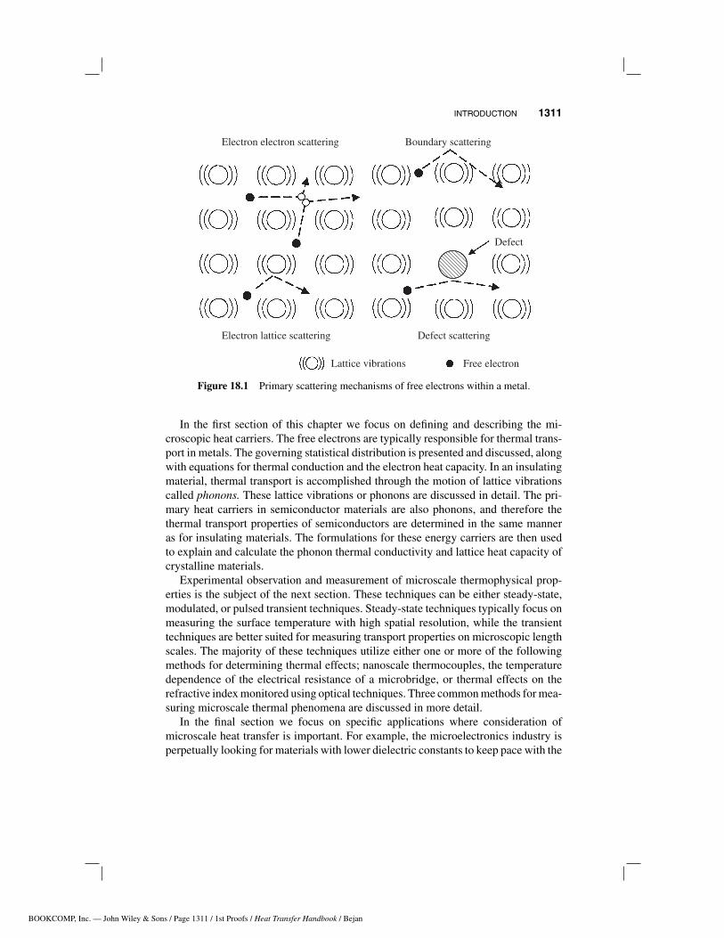
Figure 18.4 Plot of the frequency of a plane wave propagating in the crystal as a function ofwavevector. Note that the relationship is linear until k 1/a.
where M is the mass of an individual atom. By taking the time dependence of thesolution to be of the form exp(−iωt), the frequency of the solution as a function ofthe wavevector can be determined as given by eq. (18.13). Figure 18.4 shows theresults of this equation plotted over all the values that produce independent results.Values of k larger than π/a correspond to plane waves with wavelengths less thanthe interatomic spacing. Because the atoms are located at discrete points, solutionsto the equations above yielding wavelengths less than the interatomic spacing arenot unique solutions, and these solutions can be equally well represented by long-wavelength solutions.
ω(k) =√
4K
M
∣∣∣∣ sin 1
2ka (18.13)
The results shown in Fig. 18.4 apply for a Bravais lattice in one dimension, whichcan be represented by a linear chain of identical atoms connected by springs with thesame spring constant, K . A Bravais lattice with a two-point basis can be representedin one dimension by either a linear chain of alternating masses M1 and M2, separatedby a constant spring constant K , or by a linear chain of constant masses M , with thespring constant of every other spring alternating between K1 and K2. The theoreticalresults are similar in both cases, but only the case of a linear chain with atomsconnected by two different springs, K1 and K2, where the springs alternate betweenthe atoms, is discussed. The results are shown in Fig. 18.5. The displacement of eachatom from each equilibrium point is given by either u(na) for atoms with the K1
spring on their right and v(na) for atoms with the K1 spring on their left.The reason for selecting this case is its similarity to the diamond structure. Recall
that the diamond structure is a FCC Bravais lattice with a two-point basis; all theatoms are identical, but the spacing between atoms varies. As the distance varies

BOOKCOMP, Inc. — John Wiley & Sons / Page 1319 / 1st Proofs / Heat Transfer Handbook / Bejan
MICROSCOPIC DESCRIPTION OF SOLIDS 1319
123456789101112131415161718192021222324252627282930313233343536373839404142434445
[1319], (11)
Lines: 277 to 303
———0.26512pt PgVar———Normal Page
* PgEnds: Eject
[1319], (11)
n 1 n 1 n 2n
K1 K2
au na( ) v na( )
( )a
( )b
R = na
Figure 18.5 (a) One-dimensional Bravais lattice with two atoms per primitive cell shown intheir equilibrium positions. The atoms are identical in mass; however, the atoms are connectedby springs with alternating strengths K1 and K2. (b) One-dimensional Bravais lattice with twoatoms per primitive cell where the atoms are displaced by u(na) and v(na).
between atoms, so do the intermolecular forces, which are represented here by twodifferent spring constants. The equations of motion for this system are given by
Md2un
dt2= −K1(un − vn) − K2(un − vn−1) (18.14a)
Md2vn
dt2= −K1(vn − un) − K2(vn − un+1) (18.14b)
where un and vn represent the displacement of the first and second atoms within theprimitive cell, andK1 andK2 are the spring constants of the alternating springs. Againtaking the time dependence of the solution to be of the form e−iax , the frequency ofthe solutions as a function of the wavevector can be determined as given by eq. (18.15)and shown in Fig. 18.6, assuming that K2 > K1:
ω2 = K1 + K2
M± 1
M
√K2
1 + K22 + 2K1K2 cos ka (18.15)
The expression relating the lattice vibrational frequency ω and wavevector k istypically called the dispersion relation. There are several significant differences be-tween the dispersion relation for a Bravais lattice without a basis [eq. (18.13)] versusa lattice with a basis [eq. (18.15)]. One of the most valuable pieces of informationthat can be gathered from the dispersion relation is the group velocity. The groupvelocity vg governs the rate of energy transport within a material and is given by theexpression
vg = ∂ω
∂k(18.16)

BOOKCOMP, Inc. — John Wiley & Sons / Page 1320 / 1st Proofs / Heat Transfer Handbook / Bejan
1320 MICROSCALE HEAT TRANSFER
123456789101112131415161718192021222324252627282930313233343536373839404142434445
[1320], (12)
Lines: 303 to 320
———0.04701pt PgVar———Normal Page
PgEnds: TEX
[1320], (12)
a
a
Wavevector, k
Optical
Acoustic
2K
M
2 2K
M
2
2( )K K
M
2 22K
M
1 2K
M
1
( )k
0
Figure 18.6 Dispersion relation for a one-dimensional Bravais lattice with a two-point basis.
The dispersion relations shown in Fig. 18.4 and in the lower curve in Fig. 18.6 areboth roughly linear until k 1/a, at which point the slope decreases and vanishesat the edge of the Brillouin zone, where k = π/a. From these dispersion relationsit can be observed that the group velocity stays constant for small values of k andgoes to zero at the edge of the Brillouin zone. It follows directly that waves withsmall values of k, corresponding to longer wavelengths, contribute significantly to thetransport of energy within the material. These curves represent the acoustic branch ofthe dispersion relation because plane waves with small k, or long wavelength, obey alinear dispersion relation ω = ck, where c is the speed of sound or acoustic velocity.
The upper curve shown in Fig. 18.6 is commonly referred to as the optical branchof the dispersion relation. The name comes from the fact that the higher frequenciesassociated with these vibrational modes enable some interesting interactions withlight at or near the visible spectrum. The group velocity of these waves is typicallymuch less than for the acoustic branch. Therefore, contributions from the opticalbranch are usually considered negligible when evaluating the transport properties.Contributions from the optical branch must be considered when evaluating the spe-cific heat.
Dispersion relations for a three-dimensional crystal in a particular direction willlook very similar to one-dimensional relations except that there are transverse modes.The transverse modes arise due to the shear waves that can propagate in a three-dimensional crystal. The two transverse modes travel at velocities slower than thelongitudinal mode; however, they still contribute to the transport properties. Theoptical branch can also have transverse modes. Again, optical branches occur only inthree-dimensional Bravais lattices with a basis and do not contribute to the transportproperties, due to their low group velocities.
Figure 18.7 shows the dispersion relations for lead at 100 K (Brockhouse et al.,1962). This is an example of a monoatomic Bravais lattice, since lead has a face-centered cubic (FCC) crystalline structure. Therefore, there are only acousticbranches, one longitudinal branch and two transverse. In the [110] direction it is

BOOKCOMP, Inc. — John Wiley & Sons / Page 1321 / 1st Proofs / Heat Transfer Handbook / Bejan
MICROSCOPIC DESCRIPTION OF SOLIDS 1321
123456789101112131415161718192021222324252627282930313233343536373839404142434445
[1321], (13)
Lines: 320 to 334
———0.69215pt PgVar———Normal Page
* PgEnds: Eject
[1321], (13)
Figure 18.7 Dispersion relation for lead at 100 K plotted in the [110] and [100] directions.(From Brockhouse et al., 1962.)
possible to distinguish between the two transverse modes; however, due to the sym-metry of the crystal, the two transverse modes happen to be identical in the [100]direction (Ashcroft and Mermin, 1976).
Finally, the concept of phonons must be introduced. The term phonon is commonlyused in the study of the transport properties of the crystalline lattice. The definitionof a phonon comes directly from the equation for the total internal energy Ul of avibrating crystal:
Ul =∑k,s
[ns(k) + 1
2
]hω(k, s) (18.17)
The simple explanation of eq. (18.17) is that the crystal can be seen as a collectionof 3N simple harmonic oscillators, where N is the total number of atoms withinthe system and there are three modes of oscillation, one longitudinal and two trans-verse. Using quantum mechanics, one can derive the allowable energy levels for asimple harmonic oscillator, which is exactly the expression within the summationof eq. (18.17). The summation is taken over the allowable phonon wavevectors kand the three modes of oscillation s. The definition of a phonon comes from the fol-lowing statement: The integer quantity ns(k) is the mean number of phonons withenergy hω(k, s). Therefore, the number of phonons at a particular frequency simplyrepresents the amplitude to which that vibrational mode is excited. Phonons obeythe Bose–Einstein statistical distribution; therefore, the number of phonons with aparticular frequency ω at an equilibrium temperature T is given by the equation
ns(k) = 1
ehω(k,s)/kBT − 1(18.18)
BOOKCOMP, Inc. — John Wiley & Sons / Page 1322 / 1st Proofs / Heat Transfer Handbook / Bejan
1322 MICROSCALE HEAT TRANSFER
123456789101112131415161718192021222324252627282930313233343536373839404142434445
[1322], (14)
Lines: 334 to 377
———1.26297pt PgVar———Long Page
PgEnds: TEX
[1322], (14)
where kB is the Boltzmann constant. Most thermal engineers are familiar with theconcept of photons. Photons also obey the Bose–Einstein distribution; therefore, thereare many conceptual similarities between phonons and photons.
The ability to calculate the energy stored within the lattice is important in anyanalysis of microscale heat transfer. Often, the calculations, which can be quite cum-bersome, can be simplified by integrating over the allowable energy states. Theseintegrations are actually performed over frequency, which is linearly related to en-ergy through Planck’s constant. The specific internal energy of the lattice, ul , is thengiven by the equation
ul =∑s
∫Ds(ω)ns(ω)hωs ∂ωs (18.19)
where Ds(ω) is the phonon density of states, which is the number of phonon stateswith frequency between ω and (ω + dω) for each phonon branch designated by s.The actual density of states of a phonon system can be calculated from the measureddispersion relation; although often, simplifying assumptions are made for the densityof states that will produce reasonable results.
18.2.5 Heat Capacity
The rate of thermal transport within a material is governed by the thermal diffusivity,which is the ratio of the thermal conductivity to the heat capacity. The heat capacityof a material is thus of critical importance to thermal performance. In this section theheat capacity of crystalline materials is examined. An understanding of the heat ca-pacity of the different energy carriers, electrons and phonons, is important in the fol-lowing section, where thermal conductivity is discussed. The heat capacity is definedas the change in internal energy of a material resulting from a change in temperature.The energy within a crystalline material, which is a function of temperature, is storedin the free electrons of a metal and within the lattice in the form of vibrational energy.
Electron Heat Capacity To solve for the electron heat capacity of a free electronmetal, Ce, the derivative of the internal energy, stored within the electron system, istaken with respect to temperature:
Ce = ∂ue
∂T= ∂
∂T
∫ ∞
0εD(ε)f (ε) dε (18.20)
The only temperature-dependent term within this integral is the Fermi–Dirac distribu-tion. Therefore, the integral can be simplified, yielding an expression for the electronheat capacity:
Ce = π2k2Bne
2εFT (18.21)
where Ce is a linear function of temperature and ne is the electron number density.The approximations made in the simplification of foregoing integral hold for electrontemperatures above the melting point of the metal.

BOOKCOMP, Inc. — John Wiley & Sons / Page 1323 / 1st Proofs / Heat Transfer Handbook / Bejan
MICROSCOPIC DESCRIPTION OF SOLIDS 1323
123456789101112131415161718192021222324252627282930313233343536373839404142434445
[1323], (15)
Lines: 377 to 408
———1.28397pt PgVar———Long Page
PgEnds: TEX
[1323], (15)
Phonon Heat Capacity Deriving an expression for the heat capacity of a crystalis slightly more complicated. Again, the derivative of the internal energy, storedwithin the vibrating lattice, is taken with respect to temperature:
Cl = ∂ul
∂T= ∂
∂T
[∑s
∫Ds(ω)ns(ω)hωs∂ω
](18.22)
To calculate the lattice heat capacity, an expression for the phonon density of statesis required. There are two common models for the density of states of the phononsystem, the Debye model and the Einstein model. The Debye model assumes that allthe phonons of a particular mode, longitudinal or transverse, have a linear dispersionrelation. Because longer-wavelength phonons actually obey a linear dispersion rela-tion, the Debye model predominantly captures the effects of the longer-wavelengthphonons. In the Einstein model, all the phonons are assumed to have the same fre-quency and hence the dispersion relation is flat; this assumption is thus more repre-sentative of optical phonons. Because both optical and acoustic phonons contributeto the heat capacity, both models play a role in explaining the heat capacity. However,the acoustic phonons alone contribute to the transport properties; therefore, the Debyemodel will typically be used for calculating the transport properties.
Debye Model The basic assumption of the Debye model is that the dispersionrelation is linear and all three acoustic branches have the speed of sound c:
ω(k) = ck (18.23)
However, unlike photons, this dispersion relation does not extend to infinity. Sincethere are only N primitive cells within the lattice, there are only N independentwavevectors for each acoustic mode. Using spherical coordinates again, conceiveof a sphere of radius kD in wavevector space, where the total number of allowablewavevectors within the sphere must be N and each individual wavevector occupies avolume of (2π/L)3:
4
3πk3
D = N
(2π
L
)3
→ kD =(
6π2N
V
)1/3
(18.24)
Using eq. (18.24), the maximum frequency allowed by the Debye model, known asthe Debye cutoff frequency ωD , is
ωD = c
(6π2N
V
)1/3
(18.25)
Now that the maximum frequency allowed by the Debye model is known and it isassumed that the dispersion relation is linear, an expression for the phonon densityof states is required. Again, the concept of a sphere in wavevector space can beused to find the number of allowable phonon modes N with wavevector less than k.Each allowable wavevector occupies a volume in reciprical space equal to (2π/L)3.
BOOKCOMP, Inc. — John Wiley & Sons / Page 1324 / 1st Proofs / Heat Transfer Handbook / Bejan
1324 MICROSCALE HEAT TRANSFER
123456789101112131415161718192021222324252627282930313233343536373839404142434445
[1324], (16)
Lines: 408 to 452
———3.40015pt PgVar———Normal Page
PgEnds: TEX
[1324], (16)
Therefore, the total volume of the sphere of radius k must be equal to the number ofphonon modes with wavevector less than k multiplied times (2π/L)3:
4
3πk3 = N
(2π
L
)3
→ N = V
6π2k3 (18.26)
The phonon density of states D(ω) is the number of allowable states at a particularfrequency and can be determined by the expression
D(ω) = ∂N
∂ω= V
2π2c3ω2 (18.27)
Returning to eq. (18.22), all the information needed to calculate the lattice heatcapacity is known. Again simplifying the problem by assuming that all three acousticmodes obey the same dispersion relation, ω(k) = ck, the lattice heat capacity can becalculated using
Cl(T ) = 3V h2
2π2c3kBT 2
∫ ωD
0ω4 ehω/kBT
(ehω/kBT − 1)2dω (18.28)
which can be simplified further by introducing a term called the Debye temperature,θD . The Debye temperature is calculated directly from the Debye cutoff frequency,
kBθD = hωD → θD = hωD
kB(18.29)
With this new quantity, the lattice specific heat calculated under the assumptions ofthe Debye model can be expressed as
Cl(T ) = 9NkB
(T
θD
)3 ∫ θD/T
0
x4ex
(ex − 1)2dx (18.30)
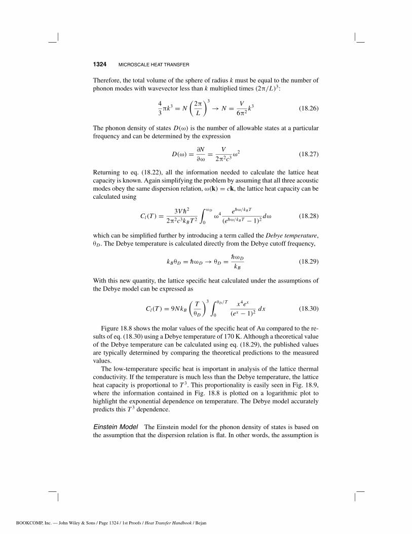
Figure 18.8 shows the molar values of the specific heat of Au compared to the re-sults of eq. (18.30) using a Debye temperature of 170 K. Although a theoretical valueof the Debye temperature can be calculated using eq. (18.29), the published valuesare typically determined by comparing the theoretical predictions to the measuredvalues.
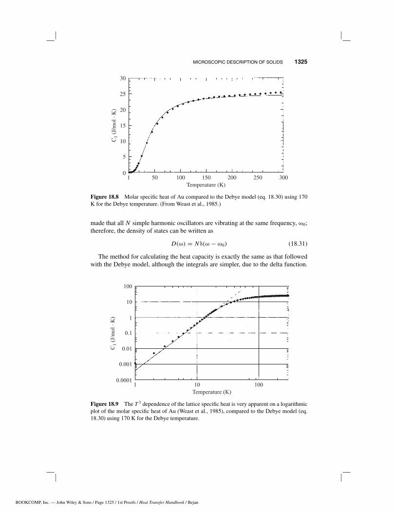
The low-temperature specific heat is important in analysis of the lattice thermalconductivity. If the temperature is much less than the Debye temperature, the latticeheat capacity is proportional to T 3. This proportionality is easily seen in Fig. 18.9,where the information contained in Fig. 18.8 is plotted on a logarithmic plot tohighlight the exponential dependence on temperature. The Debye model accuratelypredicts this T 3 dependence.
Einstein Model The Einstein model for the phonon density of states is based onthe assumption that the dispersion relation is flat. In other words, the assumption is
BOOKCOMP, Inc. — John Wiley & Sons / Page 1325 / 1st Proofs / Heat Transfer Handbook / Bejan
MICROSCOPIC DESCRIPTION OF SOLIDS 1325
123456789101112131415161718192021222324252627282930313233343536373839404142434445
[1325], (17)
Lines: 452 to 466
———0.024pt PgVar———Normal Page
PgEnds: TEX
[1325], (17)
Figure 18.8 Molar specific heat of Au compared to the Debye model (eq. 18.30) using 170K for the Debye temperature. (From Weast et al., 1985.)
made that all N simple harmonic oscillators are vibrating at the same frequency, ω0;therefore, the density of states can be written as
D(ω) = Nδ(ω − ω0) (18.31)
The method for calculating the heat capacity is exactly the same as that followedwith the Debye model, although the integrals are simpler, due to the delta function.
1 10 1000.0001
0.01
0.1
0.001
1
100
10
Temperature (K)
C(J
/mol
.K
)1
Figure 18.9 The T 3 dependence of the lattice specific heat is very apparent on a logarithmicplot of the molar specific heat of Au (Weast et al., 1985), compared to the Debye model (eq.18.30) using 170 K for the Debye temperature.

BOOKCOMP, Inc. — John Wiley & Sons / Page 1326 / 1st Proofs / Heat Transfer Handbook / Bejan
1326 MICROSCALE HEAT TRANSFER
123456789101112131415161718192021222324252627282930313233343536373839404142434445
[1326], (18)
Lines: 466 to 496
———2.66003pt PgVar———Short Page
PgEnds: TEX
[1326], (18)
This model provides better results than the Debye model for elements with the di-amond structure. One reason for the improvement is the optical phonons in thesematerials. Optical phonons have a roughly flat dispersion relation, which is betterrepresented by the Einstein model.
18.2.6 Thermal Conductivity
The specific energy carriers have been discussed in previous sections. The mannerin which these carriers store energy, and the appropriate statistics that describe theenergy levels that they occupy, have been presented. In the next section we focuson how these carriers transport energy and the mechanisms that inhibit the flow ofthermal energy. Using very simple arguments from the kinetic theory of gases, anexpression for the thermal conductivity K can be obtained:
K = 13Cvl (18.32)
where C is the heat capacity of the particle, v the average velocity of the particles,and l the mean free path or average distance between collisions.
Electron Thermal Conductivity in Metals Thermal conduction within metalsoccurs due to the motion of free electrons within the metal. According to eq. (18.32),there are three factors that govern thermal conduction: the heat capacity of the energycarrier, the average velocity, and the mean free path. As shown in eq. (18.21), theelectron heat capacity is linearly related to temperature. As for the velocity of theelectrons, the Fermi–Dirac distribution, eq. (18.7), dictates that the only electronswithin a metal that are able to undergo transitions, and thereby transport energy, arethose located at energy levels near the Fermi energy. The energy contained with theelectron system is purely kinetic and can therefore be converted into velocity. Becauseall electrons involved in transport of energy have an amount of kinetic energy close tothe Fermi energy, they are all traveling at velocities near the Fermi velocity. Therefore,the assumption is made that all the electrons within the metal are traveling at the Fermivelocity, which is given by
vF =√
2
mεF (18.33)
The third important contributor to the thermal conductivity is the electron meanfree path, obviously a direct function of the electron collisional frequency. Electroncollisions can occur with other electrons, the lattice, defects, grain boundaries, andsurfaces. Assuming that each scattering mechanism is independent, Matthiessen’srule states that the total collisional rate is simply the sum of the individual scatteringmechanisms (Ziman, 1960):
νtot = νee + νep + νd + νb (18.34)
BOOKCOMP, Inc. — John Wiley & Sons / Page 1327 / 1st Proofs / Heat Transfer Handbook / Bejan
MICROSCOPIC DESCRIPTION OF SOLIDS 1327
123456789101112131415161718192021222324252627282930313233343536373839404142434445
[1327], (19)
Lines: 496 to 515
———0.25099pt PgVar———Short Page
PgEnds: TEX
[1327], (19)
where νee is the electron–electron collisional frequency, νep the electron–latticecollisional frequency, νd the electron–defect collisional frequency, and νb the elec-tron–boundary collisional frequency. Consideration of each of these scattering mech-anisms is important in the area of microscale heat transfer.
The temperature dependence of the collisional frequency can also be very im-portant. Electron–defect and electron–boundary scattering are both typically inde-pendent of temperature, whereas for temperatures above the Debye temperature, theelectron–lattice collisional frequency is proportional to the lattice temperature. Elec-tron–electron scattering is proportional to the square of the electron temperature:
νee AT 2e νep = BTl (18.35)
where A and B are constant coefficients and Te and Tl are the electron and latticetemperatures. In clean samples at low temperatures, electron–lattice scattering dom-inates. However, electron–lattice scattering occurs much less frequently than simplekinetic theory would predict. In very pure samples and at very low temperatures, themean free path of an electron can be as long as several centimeters, which is morethan 108 times the distance between lattice sites. This is because the electrons do notscatter directly off the ions, due to the wavelike nature that allows the electrons totravel freely within the periodic structure of the lattice. Scattering occurs only whenthere are disturbances in the periodic structure of the lattice.
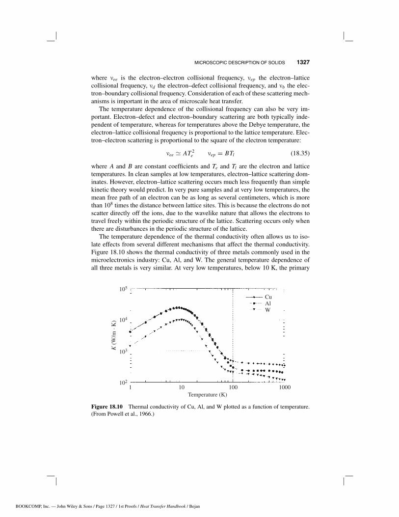
The temperature dependence of the thermal conductivity often allows us to iso-late effects from several different mechanisms that affect the thermal conductivity.Figure 18.10 shows the thermal conductivity of three metals commonly used in themicroelectronics industry: Cu, Al, and W. The general temperature dependence ofall three metals is very similar. At very low temperatures, below 10 K, the primary
Figure 18.10 Thermal conductivity of Cu, Al, and W plotted as a function of temperature.(From Powell et al., 1966.)

BOOKCOMP, Inc. — John Wiley & Sons / Page 1328 / 1st Proofs / Heat Transfer Handbook / Bejan
1328 MICROSCALE HEAT TRANSFER
123456789101112131415161718192021222324252627282930313233343536373839404142434445
[1328], (20)
Lines: 515 to 538
———0.0pt PgVar———Normal Page
PgEnds: TEX
[1328], (20)
scattering mechanism is due to either defect or boundary scattering, both of whichare independent of temperature. The linear relation between the thermal conductivityand temperature in this regime arises from the linear temperature dependence of theelectron heat capacity. At temperatures above the Debye temperature, the thermalconductivity is roughly independent of temperature as a result of competing temper-ature effects. The electron heat capacity is still linearly increasing with temperature[eq. (18.21)], but the mean free path is inversely proportional to temperature, due toincreased electron–lattice collisions, as indicated by eq. (18.35).
LatticeThermal Conductivity Thermal conduction within the crystalline latticeis due primarily to acoustic phonons. The original definition of phonons was based onthe amplitude of a particular vibrational mode and that the energy contained within aphonon was finite. In this section, phonons are treated as particles, which is analogousto assuming that the phonon is a localized wave packet. Acoustic phonons generallyfollow a linear dispersion relation; therefore, the Debye model will generally beadopted when modeling the thermal transport properties, and the group velocity isassumed constant and equal to the speed of sound within the material. Thus, all thephonons are assumed to be traveling at a velocity equal to the speed of sound, whichis independent of temperature. At very low temperatures the phonon heat capacityis proportional to T 3, while at temperatures above the Debye temperature, the heatcapacity is nearly constant.
The kinetic theory equation for the thermal conductivity of a diffusive system,eq. (18.32), is also very useful for understanding conduction in a phonon system.However, for this equation to be applicable, the phonons must scatter with each other,defects, and boundaries. If these interactions did not occur, the transport would bemore radiative in nature. In some problems of interest in microscale heat transfer,the dimensions of the system are small enough that this is actually the case, andfor these problems a model was developed called the equations of phonon radiativetransport (Majumdar, 1993). However, in bulk materials, the phonons do scatter andthe transport is diffusive. The phonons travel through the system much like waves,so it is easy to envision reflection and scattering occurring when waves encountera change in the elastic properties of the material. Boundaries and defects obviouslyrepresent changes in the elastic properties. The manner in which scattering occursbetween phonons is not as straightforward.
Two types of phonon–phonon collisions occur within crystals, described by eitherthe normal or N process or the Umklapp or U process. In the simplest case, twophonons with wavevectors k1 and k2 collide and combine to form a third phononwith wavevector k3. This collision must conserve energy:
hω(k1) + hω(k2) = hω(k3) (18.36)
Previously, the reciprocal lattice vector was defined as a vector through which anyperiodic property can be translated and still result in the same value. Since the dis-persion relation is periodic throughout the reciprocal lattice,
hω(k) = hω(k + b) (18.37)
BOOKCOMP, Inc. — John Wiley & Sons / Page 1329 / 1st Proofs / Heat Transfer Handbook / Bejan
MICROSCOPIC DESCRIPTION OF SOLIDS 1329
123456789101112131415161718192021222324252627282930313233343536373839404142434445
[1329], (21)
Lines: 538 to 574
———0.15703pt PgVar———Normal Page
PgEnds: TEX
[1329], (21)
can be written. Here, b is the reciprocal lattice vector. If eq. (18.37) is substituted intoeq. (18.36) and a linear dispersion relation is assumed, ω(k) = ck, then
k1 + k2 = k3 + b (18.38)
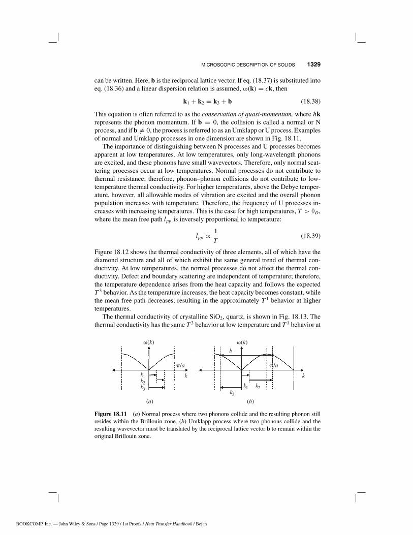
This equation is often referred to as the conservation of quasi-momentum, where hkrepresents the phonon momentum. If b = 0, the collision is called a normal or Nprocess, and if b = 0, the process is referred to as an Umklapp or U process. Examplesof normal and Umklapp processes in one dimension are shown in Fig. 18.11.
The importance of distinguishing between N processes and U processes becomesapparent at low temperatures. At low temperatures, only long-wavelength phononsare excited, and these phonons have small wavevectors. Therefore, only normal scat-tering processes occur at low temperatures. Normal processes do not contribute tothermal resistance; therefore, phonon–phonon collisions do not contribute to low-temperature thermal conductivity. For higher temperatures, above the Debye temper-ature, however, all allowable modes of vibration are excited and the overall phononpopulation increases with temperature. Therefore, the frequency of U processes in-creases with increasing temperatures. This is the case for high temperatures, T > θD ,where the mean free path lpp is inversely proportional to temperature:
lpp ∝ 1
T(18.39)
Figure 18.12 shows the thermal conductivity of three elements, all of which have thediamond structure and all of which exhibit the same general trend of thermal con-ductivity. At low temperatures, the normal processes do not affect the thermal con-ductivity. Defect and boundary scattering are independent of temperature; therefore,the temperature dependence arises from the heat capacity and follows the expectedT 3 behavior. As the temperature increases, the heat capacity becomes constant, whilethe mean free path decreases, resulting in the approximately T 1 behavior at highertemperatures.
The thermal conductivity of crystalline SiO2, quartz, is shown in Fig. 18.13. Thethermal conductivity has the same T 3 behavior at low temperature and T 1 behavior at
Figure 18.11 (a) Normal process where two phonons collide and the resulting phonon stillresides within the Brillouin zone. (b) Umklapp process where two phonons collide and theresulting wavevector must be translated by the reciprocal lattice vector b to remain within theoriginal Brillouin zone.

BOOKCOMP, Inc. — John Wiley & Sons / Page 1330 / 1st Proofs / Heat Transfer Handbook / Bejan
1330 MICROSCALE HEAT TRANSFER
123456789101112131415161718192021222324252627282930313233343536373839404142434445
[1330], (22)
Lines: 574 to 578
———-3.32802pt PgVar———Normal Page
PgEnds: TEX
[1330], (22)
Figure 18.12 Thermal conductivity of the diamond structure shown as a function of temper-ature. (From Powell et al., 1974.)
Figure 18.13 Thermal conductivity of crystalline and amorphous forms of SiO2. (FromPowell et al., 1966.)
high temperature. The thermal conductivity is plotted for the direction parallel to thec-axis because quartz has a hexagonal crystalline structure. The thermal conductivityof fused silica, also shown in Fig. 18.13, does not follow this behavior since itis an amorphous material and does not have a crystalline structure. The thermalconductivity of amorphous materials is an entirely different subject, and the readeris referred to several good references on the subject, such as Cahill and Pohl (1988)and Mott (1993).

BOOKCOMP, Inc. — John Wiley & Sons / Page 1331 / 1st Proofs / Heat Transfer Handbook / Bejan
MODELING 1331
123456789101112131415161718192021222324252627282930313233343536373839404142434445
[1331], (23)
Lines: 578 to 603
———-1.72595pt PgVar———Normal Page
* PgEnds: Eject
[1331], (23)
18.3 MODELING
Now that an understanding of the basic energy, carriers and the statistical proceduresfor dealing with these carriers has been developed, in this section we focus on adiscussion of the methods for modeling heat transfer on the microscale. The first andsimplest approach is to modify the continuum models to incorporate microscale heattransfer effects. Typically, continuum models can be used as long as meaningful localtemperatures can be established. The next approach is to make use of the Boltzmanntransport equation (Majumdar, 1998). With this approach, the transport equationsdeveloped are no longer dependent on temperature but on the statistical distributionsof the energy carriers. The collisional term in the Boltzmann transport equation,however, is very difficult to model, and the assumptions made when modeling thisterm eventually limit the accuracy of this approach. Finally, the transport of thermalenergy can be modeled using more molecular approaches, such as lattice dynamics,molecular dynamics, and Monte Carlo simulations (Klistner et al., 1988; Chou et al.,1999; Tamura et al., 1999). These approaches are the most fundamental in concept;however, they are computationally difficult and are ultimately limited by knowledgeof the intermolecular forces between the atoms.
18.3.1 Continuum Models
Microscale heat transfer continuum models can be separated in several categories,depending on the basic transport mechanisms and the type of energy carriers involved.The first distinction is based on the manner in which heat transport occurs. If theenergy carrier undergoes frequent collisions, transport is diffusive and the heat fluxq is given by Fourier’s law:
q = −K ∇T (18.40)
whereK is the thermal conductivity. When eq. (18.40) is combined with the conserva-tion of energy equation, the result is a parabolic differential equation. One theoreticalproblem with Fourier’s law is that it yields an infinite speed of propagation of thermalenergy. In order words, if the surface of a material is instantaneously heated, Fourier’slaw dictates that the thermal effect is felt immediately throughout the entire system.Typically, this effect is extremely small, and the speed with which the average of thethermal energy density travels is actually quite slow. Consider the one-dimensionalheat equation for an instantaneous pulse that arrives at the surface at time zero:
C∂T
∂t(x, t) = ∂
∂x(q) + Soδ(x)δ(t) (18.41)
whereC is the heat capacity of the material, x the direction of heat flow, So the amountof energy deposited, and δ is a delta function. The solution to this problem is givenby (Kittel and Kroemer, 1980)
T (x, t) = 2So
C
√4πDt exp
(−x2
4Dt
)(18.42)

BOOKCOMP, Inc. — John Wiley & Sons / Page 1332 / 1st Proofs / Heat Transfer Handbook / Bejan
1332 MICROSCALE HEAT TRANSFER
123456789101112131415161718192021222324252627282930313233343536373839404142434445
[1332], (24)
Lines: 603 to 638
———0.00703pt PgVar———Long Page
PgEnds: TEX
[1332], (24)
Figure 18.14 Time rate of change of the root mean square of the distance to which the effectsof the instantaneous pulse have propagated plotted as a function of time.
where D is the thermal diffusivity of the material. The root mean square of thedistance to which the effects of the instantaneous pulse have propagated is given by
xrms(t) = √2Dt (18.43)
Taking the derivative of this expression yields the average velocity with which thethermal energy propagates. Figure 18.14 shows the time rate of change of xrms plottedversus time for Au at two different temperatures. In the low-temperature case, the timerate of change of xrms, which represents the velocity of the energy carriers, exceedsthe Fermi velocity for the first several hundred picoseconds. It is not possible for thethermal energy to propagate at this rate because the Fermi velocity represents thespeed of the electrons. This illustrates that a time scale exists where a finite speed ofpropagation much be considered.
Catteneo’s equation was introduced to account for the finite speed of thermalenergy propagation (Joseph and Preziosi, 1989). Essentially, Catteneo’s equationaccounts for the time required for the heat flux to develop after a temperature gradienthas been applied and is given by
1
τ
∂q
∂t+ q = −K ∇T (18.44)
where τ is the relaxation time of the heat carrier. When this heat flux equationis combined with the conservation of energy equation, the result is a hyperbolicdifferential equation. This equation reduces to Fourier’s law when the relaxation timeis much less than the time scale of interest.
Another manner in which continuum thermal models have been modified to ac-count for microscale heat transfer phenomena deals with equilibrium versus nonequi-librium systems. There are instances when multiple energy carriers may be involved
BOOKCOMP, Inc. — John Wiley & Sons / Page 1333 / 1st Proofs / Heat Transfer Handbook / Bejan
MODELING 1333
123456789101112131415161718192021222324252627282930313233343536373839404142434445
[1333], (25)
Lines: 638 to 686
———6.40465pt PgVar———Long Page
PgEnds: TEX
[1333], (25)
in a problem, and the representative temperature of each energy carrier system is dif-ferent. Ultrashort pulsed laser heating and nonequilibrium Joule heating in field-effecttransistors are two examples where nonequilibrium thermal systems occur. During ul-trashort pulsed laser heating of metals, the electron and phonon systems can be treatedseparately. The conservation of energy equations for both systems are given by
Ce(Te)∂Te
∂t= ∇(qe) + G(Te − Tl) + Se (18.45a)
Cl(Tl)∂Tl
∂t= ∇(ql) − G(Te − Tl) + Sl (18.45b)
where G(Te − Tl) is the rate of energy exchange between the two systems, G theelectron–phonon coupling factor, and Se and Sl are the source terms for the electronand lattice systems, respectively. The resulting system of equations can again beparabolic or hyperbolic, depending on the appropriate equation for the heat flux, eq.(18.40) or (18.44).
Even when continuum heat transfer equations are appropriate, the thermophysicalproperties can be influenced by microscale phenomena. The thermal conductivitycan be reduced significantly due to increased defect and/or grain boundary scattering(Mayadas et al., 1969). When the length scale of the film is on the order of theheat carrier mean free path, there can be changes in the transport properties due toincreased boundary scattering (Fuchs, 1938).
18.3.2 BoltzmannTransport Equation
The Boltzmann transport equation (BTE) is simply a conservation equation, wherethe conserved quantity is the number of particles. The general form of the BTE isgiven by the following equation for classical particles (Ziman, 1960):
∂
∂t[f(x,P,t) dVx dVP] + v·∇x[f(x,P,t) dVx dVP] + F·∇P [f(x,P,t) dVx dVP]
=∂
∂t[f(x,P,t) dVx dVP]
coll
(18.46)︸ ︷︷ ︸ ︸ ︷︷ ︸ ︸ ︷︷ ︸︸ ︷︷ ︸
total time convection convection of time rate ofrate of of particles particles in change ofchange of in physical momentum number ofnumber of space space particles dueparticles to collisions
where f is the distribution of particles, dVx a differential control volume locatedat position x, and dVP a differential control volume located at momentum P . Thefirst term represents the quantity of interest, the time rate of change of the numberof particles at position x that have velocity v. The second term represents particles

BOOKCOMP, Inc. — John Wiley & Sons / Page 1334 / 1st Proofs / Heat Transfer Handbook / Bejan
1334 MICROSCALE HEAT TRANSFER
123456789101112131415161718192021222324252627282930313233343536373839404142434445
[1334], (26)
Lines: 686 to 707
———8.1921pt PgVar———Normal Page
* PgEnds: Eject
[1334], (26)
that physically cross the boundaries of the differential control volume in physicalspace. The third term accounts for particles that are acted on by an external force F
and are therefore accelerated into or out of the differential control volume in velocityspace. Finally, the right-hand side of the equation accounts for changes in positionand velocity which can occur whenever two particles collide. This equation is directlyapplicable to electrons and classical particles where the momentum is representedby P = mv. In the case of electrons, the momentum can be expressed in terms ofthe wavevector using the expression P = hk. This equation for the momentum isalso used with phonons and photons; however, momentum is not strictly conserved,eq. (18.38).
When applying eq. (18.46) in the solution of microscale heat transfer problems,the greatest difficulty comes from the collisional term on the right-hand side. Generalexpressions for the collisional frequencies of electron–electron, electron–phonon, andphonon–phonon scattering have already been presented as eqs. (18.35) and (18.39).However, the detailed nature of these collisions has not been examined fully. Typ-ically, the relaxation time approximation is utilized. Under this approximation, thefollowing expression is used:(
∂f
∂t
)collisions
= −f − fo
τ(18.47)
where fo is the equilibrium distribution and τ is the relaxation time. The relaxationtime approximation is based on the assumption of a distribution that is slightly per-turbed from its equilibrium distribution f such that the distribution function can bewritten as f = fo + f ′. Collisions within the system will then act to bring about anequilibrium distribution. Substituting this expression into eq. (18.47) and solving forthe deviation from equilibrium as a function of time due solely to collisional effectsyields
∂f ′
∂t= −f ′
τ→ f ′(t) = et/τ (18.48)
Therefore, by using eq. (18.47) for the collisional term, the assumption has been madethat the collisions within the system will bring any deviation back to equilibrium ac-cording to an exponential decay. The relaxation time τ is simply the time required forthe collisional effects to decrease the deviation by a factor of 1/e. Although the re-laxation time is not exactly the mean free time between collisions, the two are oftenassumed to be of the same order of magnitude and will sometimes be used inter-changeably. When multiple relaxation times are applicable, such as electron–latticeand electron–defect scattering, they may be combined by again using Mathiessen’srule, eq. (18.34), assuming that the collisional mechanisms are independent. Note thatthe relaxation time is inversely proportional to the collisional frequency.
Phonons A general form of the Boltzmann transport equation for a phonon systemis given by

BOOKCOMP, Inc. — John Wiley & Sons / Page 1335 / 1st Proofs / Heat Transfer Handbook / Bejan
MODELING 1335
123456789101112131415161718192021222324252627282930313233343536373839404142434445
[1335], (27)
Lines: 707 to 750
———3.01219pt PgVar———Normal Page
* PgEnds: Eject
[1335], (27)
∂
∂t[N(x,k, t) dVx dVk] + v · ∇x [N(x,k, t) dVx dVk]
= −(N(x,k, t) − No(x,k, t)
τ
)(18.49)
where N(x,k, t) is the Bose-Einstein distribution as a function of position, wavevec-tor, and time, and hk is used to express the quasi-momentum of the phonon. Theassumption is made that no external forces act on the phonons within the crystal.Using this form, the rate of heat transfer due to phonons can be determined withina crystal under a steady-state temperature gradient applied in the x direction. Theone-dimensional Boltzmann transport equation can be written as
vx∂N
∂x= −N − No
τ(18.50)
Thermal transport within the crystal occurs due to slight deviations from an equilib-rium distribution, N = No + N . The assumption that ∂No/∂x ∂N/∂x yields
N = −vxτ∂No
∂x(18.51)
Because the equilibrium distribution does not contribute to heat flux, f ′ yields theonly contribution. The heat flux of a phonon system can be written in terms of thenumber of electrons traveling in the x direction carrying energy hω:
qx =∫
vxN(ω)hωD(ω) dω (18.52)
where D(ω) is the phonon density of states. Substituting the expression for N givenin eq. (18.51) into eq. (18.52) yields
qx =
∫vx
(−vxτ
∂No
∂x
)hωD(ω) dω (18.53a)
∫vx
(−vxτ
∂No
∂T
∂T
∂x
)hωD(ω) dω (18.53b)
−v2xτ
[∫∂No
∂ThωD(ω) dω
]dT
dx(18.53c)
The expression inside the brackets in eq. (18.53c) is, by definition, the lattice heatcapacity, eq. (18.22). The mean free path of a phonon is equal to the product ofthe mean free time between collisions and the speed of the particle, Λ = vτp. Thespeed of sound in the solid is equal to the square root of the sum of the three velocitycomponents squared. If all the velocity components are equal, vx = 1
3v2. Substituting
all these expressions into eq. (18.53c) gives the same expression for the thermalconductivity that was presented as eq. (18.32):
BOOKCOMP, Inc. — John Wiley & Sons / Page 1336 / 1st Proofs / Heat Transfer Handbook / Bejan
1336 MICROSCALE HEAT TRANSFER
123456789101112131415161718192021222324252627282930313233343536373839404142434445
[1336], (28)
Lines: 750 to 800
———-2.0078pt PgVar———Long Page
* PgEnds: Eject
[1336], (28)
qx = −1
3CvΛ
dT
dx(18.54)
If the problem is transient rather then steady state, the time derivative term mustbe retained in the Boltzmann transport equation. Making the same assumptions aswere made for the steady-state case, the BTE can be reduced to the form
τ∂f ′
∂t+ f ′ = −vxτ
∂fo
∂x(18.55)
This solution can then be used to derive an equation for the heat flux, which is identicalto Catteneo’s equation for hyperbolic heat conduction:
τ∂q
∂t+ q = −1
3CvΛ
∂T
∂x(18.56)
Despite this result, experience indicates that Fourier’s law is applicable for mosttransient problems. This is because in most heat transfer problems the time scaleof interest is much larger than the relaxation time of the energy carrier, in which casethe first term can be neglected.
Electrons When dealing with the transport properties of metals, such as currentdensity and thermal conduction due to the electrons, it is useful to begin with thegeneral form of the Boltzmann transport equation for an electron system as given bythe expression
∂
∂t[f (x,k,t) dVx dVk] + v · ∇x [f (x,k,t) dVx dVk] − eE
m· ∇k [f (x,k,t) dVx dVk]
=
∂
∂t[f (x,k, t) dVx dVk]
coll
(18.57)
where hk is used to express the momentum of the electron, m is the effective mass ofan electron, and the force on an electron in the presence of an electric field E is givenby F = −eE. Again assuming that there is a temperature gradient in the x directionand that the distribution is only slightly perturbed from an equilibrium distribution,the Boltzmann transport equation reduces to
f ′ = −(
vxτ∂fo
∂T
)dT
dx−
(eτ
m
∂fo
∂vx
)E (18.58)
The following equations can be used to calculate the current density j and heat fluxq of a metal based on the number of electrons traveling in a certain direction:
j =∫
e · vf (ε)D(ε) dε (18.59)
q =∫
ε · vf (ε)D(ε) dε (18.60)

BOOKCOMP, Inc. — John Wiley & Sons / Page 1337 / 1st Proofs / Heat Transfer Handbook / Bejan
MODELING 1337
123456789101112131415161718192021222324252627282930313233343536373839404142434445
[1337], (29)
Lines: 800 to 849
———4.54617pt PgVar———Long Page
* PgEnds: Eject
[1337], (29)
Again, only the deviation from the equilibrium distribution contributes to the trans-port properties. Therefore, the current density and heat flux can be written in terms ofthe thermal gradient and electrical field with four linear coefficients (Ziman, 1960):
j = LEEE + LET ∇T (18.61)
q = LTEE + LTT ∇T (18.62)
If the thermal gradient is zero, eq. (18.61) reduces to Ohm’s law, where j = σE andLEE = σ. Using eqs. (18.58) and (18.59), it is possible to solve for the electricalconductivity using the fact that ∂f/∂ε ≈ δ(ε − εF ) and ε = 1
2mv2:
σ = ne2τ
m(18.63)
If the material is electrically insulated such that j = 0 and a thermal gradient is placedacross the material, an electric field will be created within the material such that
E = Q∇T → Q = −LET
LEE
(18.64)
where Q is the thermopower of the material. Returning briefly to the case wherethe thermal gradient is zero, ∇T = 0, there is still a heat flux occurring across thematerial, as seen from
q = LTEE = Πj → Π = LTE
LEE
(18.65)
where Π is the Peltier coefficient. This ability to create a heat flux simply by passinga current through a material is the basis for thermoelectric coolers. The effect ofmicroscale heat transfer in these devices is a topic of current interest and is discussedin Section 18.5.
Whenever a thermal gradient is applied to a material with free electrons, an electricfield is established within the material. This electric field actually creates a heat fluxthat opposes the thermal gradient. Taking this effect into account yields the followingexpression for the thermal conductivity:
K = −(LTT − LTELET
LEE
)(18.66)
For most metals the electrical conductivity, LEE , is large enough that the thermo-electric effect on the thermal conductivity can be neglected. The less electricallyconducting the material, however, the more important it becomes to account for thisreduction in the thermal conductivity. If the thermoelectric effects are neglected, thethermal conductivity takes the same form as was found for the case of phonons:
K = 13CevΛ = 1
3Cev2F τ (18.67)

BOOKCOMP, Inc. — John Wiley & Sons / Page 1338 / 1st Proofs / Heat Transfer Handbook / Bejan
1338 MICROSCALE HEAT TRANSFER
123456789101112131415161718192021222324252627282930313233343536373839404142434445
[1338], (30)
Lines: 849 to 886
———0.24205pt PgVar———Long Page
PgEnds: TEX
[1338], (30)
Using the relaxation time approximation and Boltzmann transport equation expres-sions for the electrical and thermal conductivity have been derived in terms of a re-laxation time, eqs. (18.63) and (18.67). Because both quantities are related linearlyto the relaxation time, their ratio is independent of the relaxation time:
K
σ=
13 (π
2k2Bn/2εF)v2
F τ
ne2τ/m= π2
3
(kB
e
)2
T (18.68)
where eq. (18.21) is used for the electron heat capacity. This result, known as theWiedemann-Franz law, relates the electrical conductivity to the thermal conductivityfor metals at all but very low temperature. The proportionality constant is known asthe Lorentz number:
L = K
σT= π2
3
(kB
e
)2
= 2.45 × 10⁻⁸ W · Ω/K2 (18.69)
18.3.3 Molecular Approach
Recent advances in computational capabilities have increased interest in molecularapproaches to solving microscale heat transfer problems. These approaches includelattice dynamic approaches (Tamura et al., 1999), molecular dynamic approaches(Voltz and Chen, 1999; Lukes et al., 2000), and Monte Carlo simulations (Klistner etal., 1988; Woolard et al., 1993). In lattice dynamical calculations the ions are assumedto be at their equilibrium positions, and the intermolecular forces are modeled usingappropriate expressions for the types of bonds present. This technique can be veryeffective in calculating phonon dispersion relations (Tamura et al., 1999) and hasalso been applied to calculating interfacial properties (Young and Maris, 1989). It isdifficult, however, to take into account defects and grain boundaries.
The molecular dynamics approach is very similar; however, more emphasis placedon modeling the interatomic potential and the assumption of a rigid crystalline struc-ture is no longer imposed (Chou et al., 1999). Most molecular dynamics approacheshave utilized the Lennard-Jones potential:
φ(r) = 4ξ
[( rc
r
)12 −( rc
r
)6]
(18.70)
where ξ is a measure of the strength of the attractive forces and rc is a measure ofthe radius of the repulsive core. Basically, the ions attract each other with a potentialthat varies with 1/r6 at large separation; however, they become strongly repulsive atshort distance due to the Pauli exclusion principle. The noble gases in solid form havebeen shown to be well characterized by the Lennard-Jones potential; however, somemodification is typically required for use of this potential with other crystalline mate-rials. Chou et al. (1999) provide a comprehensive review of the molecular dynamicsapproaches that have been made on microscale thermophysical problems.
Monte Carlo simulation is very similar to the Boltzmann transfer equation ap-proach, in that the energy carriers are dealt with as particles. In Monte Carlo simu-lation, the particle’s trajectory begins from a particular point traveling in a random

BOOKCOMP, Inc. — John Wiley & Sons / Page 1339 / 1st Proofs / Heat Transfer Handbook / Bejan
OBSERVATION 1339
123456789101112131415161718192021222324252627282930313233343536373839404142434445
[1339], (31)
Lines: 886 to 899
———0.0pt PgVar———Long Page
PgEnds: TEX
[1339], (31)
direction and the path is calculated based on parameters that govern the collisionalbehavior of the particles. The accuracy of this approach is limited by knowledge ofthe particular collisional events. This technique has been applied to both electron(Woolard et al., 1993) and phonon systems (Klistner et al., 1988).
18.4 OBSERVATION
Numerous experimental methods have been employed to monitor microscale heattransfer phenomena. In an attempt to discuss most of these techniques in a broadercontext, the methods are grouped into two categories. The techniques are eithersteady state or transient. The steady-state techniques usually involve thermography orsurface temperature measurements. The transient techniques use either a modulatedor pulsed heating source and monitor the temperature response as a function of time inorder to measure the thermophysical properties. The next distinguishing feature is themanner in which the thermal response is observed. The three most common methodsof observing microscale thermal phenomena include thin-film thermocouples, thin-film microbridges, and optical techniques.
Nanometer-scale thermocouples are typically used in conjunction with an atomicforce microscope (AFM) (Majumdar, 1999; Shi et al., 2000). This technique is nonde-structive because the AFM brings the probe into contact with the sample very care-fully. Another series of investigators have used thin-film microbridges, which areusually thinner than 100 nm with a width that depends on the application (Cahill etal., 1994; Lee and Cahill, 1997; Borca-Tasciuc et al., 2000). This technique relies onthe fact that the electrical resistance of the microbridge is a strong function of tem-perature. Because the microbridge must be deposited onto the material of interest,this technique is neither noncontact nor nondestructive. Finally, optical techniqueshave been employed where a laser is used as either the heating source and/or thethermal probe. The thermal effects can be monitored optically in a number of differ-ent ways. One set of techniques relies on the temperature dependence of reflectanceand these techniques are referred to as thermoreflectance techniques (Paddock andEesley, 1986; Hostetler et al., 1997). The thermal expansion that results at the surfacecan also be used to deflect the probe beam, and the deflection can be related to temper-ature. These techniques are referred to as photothermal techniques (Welsh and Ristau,1995). Finally, “mirage” techniques use the fact that the air just above the surface isalso heated, which causes changes in the index of refraction that bend the probe beamby varying amounts, depending on the change in temperature (Gonzales et al., 2000).
Three different techniques are described in the next few sections. The first tech-nique is scanning thermal microscopy (STM) (Majumdar, 1999). This is an exampleof the steady-state approach using a nanometer-scale thermocouple. The thermocou-ple is fabricated onto the tip of an AFM probe. The next technique presented is the3ω technique, which uses a thin-film microbridge as both the heating source and asa thermal probe (Cahill et al., 1994). This is an example of a modulated transienttechique. The last example is the transient thermoreflectance (TTR) technique (Pad-dock and Eesley, 1986), an optical technique in which a pulsed laser is used to heatand probe the sample. This is an excellent example of a pulsed transient technique.

BOOKCOMP, Inc. — John Wiley & Sons / Page 1340 / 1st Proofs / Heat Transfer Handbook / Bejan
1340 MICROSCALE HEAT TRANSFER
123456789101112131415161718192021222324252627282930313233343536373839404142434445
[1340], (32)
Lines: 899 to 911
———0.927pt PgVar———Normal Page
PgEnds: TEX
[1340], (32)
These examples demonstrate steady-state, modulated, and pulsed transient tech-niques and the use of thin-film thermocouples, microbridges, and optical methods,respectively, although numerous other combinations or variations of these techniqueshave been used. Steady-state microbridge techniques have been used to measure ther-mal boundary resistance (Swartz and Pohl, 1987). For example, an AFM has beenused to monitor the expansion and contraction of thin-film materials, which resultsfrom a modulated heating source (Varesi and Majumdar, 1998). Lasers have beenused as modulated heating sources (Yao, 1987), and to monitor the effects of the pulseheating source on the surface temperature (Kading et al., 1994). A technique callednear-field optical thermometry was recently developed based on near-field scanningmicroscopy technology, which uses an optical heating source and seems superiorto the diffraction limit associated with far-field optical thermometry (Goodson andAsheghi, 1997).
18.4.1 Scanning Thermal Microscopy
In this section a brief introduction to scanning thermal microscopy (SThM) is pre-sented. Majumdar (1999) published a comprehensive review article that providesmore detail and historical development of SThM. Majumdar categorized the majorityof techniques into (1) thermovoltage techniques (Shi et al., 2000), (2) electrical re-sistive techniques (Fiege et al., 1999), and (3) thermal expansion techniques (Varesiand Majumdar, 1998). A single reference has been provided here for each technique,but by no means do these represent the complete literature on the subject.
The majority of SThM experiments fall into the first category of thermovoltagetechniques. These techniques require a nanometer-scale thermocouple, which is made
Figure 18.15 (a) Nanometer-scale thermocouple manufactured on the tip of a commerciallyavailable AFM cantilever; (b) micrograph of a Cr/Pt thermocouple deposited on a SiNx can-tilever. (Reproduced with permission of L. Shi and A. Majumdar, from Shi et al., 2000.)
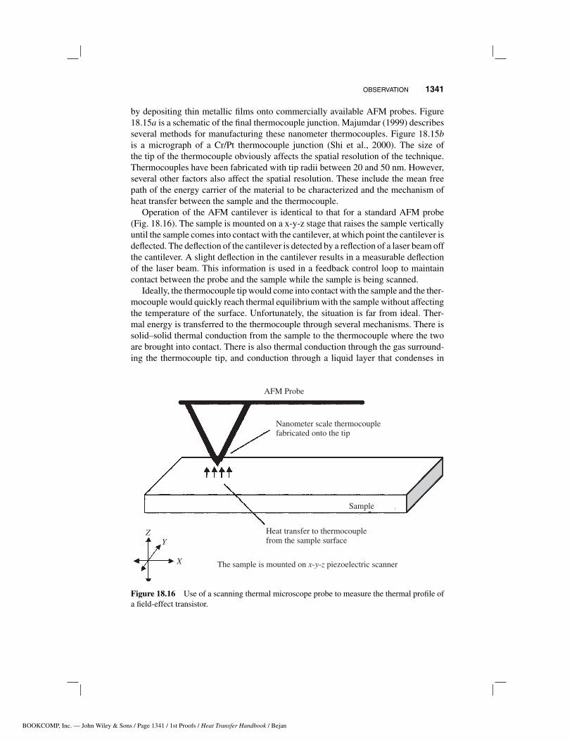
BOOKCOMP, Inc. — John Wiley & Sons / Page 1341 / 1st Proofs / Heat Transfer Handbook / Bejan
OBSERVATION 1341
123456789101112131415161718192021222324252627282930313233343536373839404142434445
[1341], (33)
Lines: 911 to 927
———1.781pt PgVar———Normal Page
PgEnds: TEX
[1341], (33)
by depositing thin metallic films onto commercially available AFM probes. Figure18.15a is a schematic of the final thermocouple junction. Majumdar (1999) describesseveral methods for manufacturing these nanometer thermocouples. Figure 18.15bis a micrograph of a Cr/Pt thermocouple junction (Shi et al., 2000). The size ofthe tip of the thermocouple obviously affects the spatial resolution of the technique.Thermocouples have been fabricated with tip radii between 20 and 50 nm. However,several other factors also affect the spatial resolution. These include the mean freepath of the energy carrier of the material to be characterized and the mechanism ofheat transfer between the sample and the thermocouple.
Operation of the AFM cantilever is identical to that for a standard AFM probe(Fig. 18.16). The sample is mounted on a x-y-z stage that raises the sample verticallyuntil the sample comes into contact with the cantilever, at which point the cantilever isdeflected. The deflection of the cantilever is detected by a reflection of a laser beam offthe cantilever. A slight deflection in the cantilever results in a measurable deflectionof the laser beam. This information is used in a feedback control loop to maintaincontact between the probe and the sample while the sample is being scanned.
Ideally, the thermocouple tip would come into contact with the sample and the ther-mocouple would quickly reach thermal equilibrium with the sample without affectingthe temperature of the surface. Unfortunately, the situation is far from ideal. Ther-mal energy is transferred to the thermocouple through several mechanisms. There issolid–solid thermal conduction from the sample to the thermocouple where the twoare brought into contact. There is also thermal conduction through the gas surround-ing the thermocouple tip, and conduction through a liquid layer that condenses in
Figure 18.16 Use of a scanning thermal microscope probe to measure the thermal profile ofa field-effect transistor.

BOOKCOMP, Inc. — John Wiley & Sons / Page 1342 / 1st Proofs / Heat Transfer Handbook / Bejan
1342 MICROSCALE HEAT TRANSFER
123456789101112131415161718192021222324252627282930313233343536373839404142434445
[1342], (34)
Lines: 927 to 942
———-1.903pt PgVar———Normal Page
PgEnds: TEX
[1342], (34)
Figure 18.17 Topographical and thermal profile of a multiwalled carbon nanotube that hasbeen heated with a dc electrical current. (Courtesy of L. Shi and A. Majumdar at the Universityof California–Berkeley.)
the small gap between the tip and the sample. Shi et al. (2000) demonstrated thatconduction through this liquid layer dominates the heat transfer under normal atmo-spheric conditions. Figure 18.17 shows a topographical and thermal image of a 10-nmmultiwalled carbon nanotube.
18.4.2 3ωTechnique
The 3ω technique has been one of the most widely used and perhaps the most effectivetechnique for measuring the thermophysical properties of dielectric thin films (Cahill,1990; Lee and Cahill, 1997). Figure 18.18a shows a top view of a microbridge usedfor the 3ω technique. Figure 18.18b shows a side view of a microbridge that hasbeen deposited onto the thin film to be measured. There are four electrical padsshown in Figure 18.18a; the outer two pads are used to send current through themicrobridge, which provides the modulated heating, while the inner two pads areused for measuring the voltage drop across the microbridge.
The current sent through the microbridge is modulated at a certain frequencywhere I = I0 cos ωt . The technique is called the 3ω technique because the tempera-ture oscillations of the sample surface from the modulated current are evident in themicrobridge voltage signal at the third harmonic of the current modulation frequency.The microbridge has a resistance R, and the power loss or Joule heating that occurswithin the system is proportional to the square of the current:

BOOKCOMP, Inc. — John Wiley & Sons / Page 1343 / 1st Proofs / Heat Transfer Handbook / Bejan
OBSERVATION 1343
123456789101112131415161718192021222324252627282930313233343536373839404142434445
[1343], (35)
Lines: 942 to 962
———0.57709pt PgVar———Normal Page
PgEnds: TEX
[1343], (35)
8 m lines
microbridge 8 m 30 nm
170 m lines
( )a ( )b
Substrate
Thin film
Figure 18.18 (a) Top view of the thin-film microbridge setup used by Lee and Cahill (1997)to measure heat transport in thin dielectric films (from Lee and Cahill, 1997); (b) microbridgedeposited onto a dielectric thin-film material. The film thickness and width are much less thanthe length of the microbridge, making the problem essentially two-dimensional.
P = I 2R = I 20 R
2(1 + cos 2ω) (18.71)
The power loss term has a steady-state component and a sinusoidal term. The modu-lated component of the heat generation occurs at a frequency of 2ω, which will resultin a temperature fluctuation within the system at a frequency of 2ω:
T (x, t) = Ts(x) + Tm(x) cos ωt (18.72)
where Ts is the steady-state temperature distribution and Tm is the amplitude of thetemperature oscillations at a frequency of 2ω. Electrical resistance in metals arisesdue to several electron scattering mechanisms, which include defect scattering, grainboundary scattering, and electron–phonon scattering. As discussed in Section 18.2,the electron–phonon collisional frequency is proportional to the lattice temperature.Therefore, the electrical resistance of metals increases linearly with temperature,R = R0+R1T . This change in the electrical resistance of the film is the basic thermalmechanism that allows for detection of the temperature changes using microbridgetechniques:
Vmb = IRmb = I0 cos ωt [R0 + R1(Ts + Tm cos 2ωt)] (18.73)
Oscillations occur within the microbridge voltage signal at frequencies of ω and 3ω,where the 3ω signal contains information about the amplitude of the temperaturefluctuations of the microbridge. The amplitude of the temperature oscillation is thencompared to a thermal model as a function of the heating frequency to determine theeffective thermal diffusivity of the underlying material.
One interesting aspect of modulated techniques is that the modulation frequencycan be varied, which affects the amount of material that influences the measurement.Essentially, higher oscillation frequencies will only probe the thermal properties near

BOOKCOMP, Inc. — John Wiley & Sons / Page 1344 / 1st Proofs / Heat Transfer Handbook / Bejan
1344 MICROSCALE HEAT TRANSFER
123456789101112131415161718192021222324252627282930313233343536373839404142434445
[1344], (36)
Lines: 962 to 990
———5.32007pt PgVar———Normal Page
PgEnds: TEX
[1344], (36)
the surface, while lower frequencies allow more time for diffusion and can be usedto probe thicker films. This effect can easily be understood by examining the one-dimensional solution to the heat equation for a semi-infinite material where accordingto Majumdar (1999), the surface temperature is being modulated at frequency ωs :
T (x, t) ∝ exp
(−x
√ωs
2αeff
)exp
[i
(ωs t − x
√ωs
2αeff
)](18.74)
where αeff is the effective thermal diffusivity of the material. These temperatureoscillations occurring throughout the film at the modulation frequency are sometimesreferred to as thermal waves (Rosencwaig et al., 1985). Notice that the amplitude ofthe temperature oscillation decays exponentially. The penetration depth is inverselyproportional to the square root of the modulation frequency:
δtw =√
2α
ω(18.75)
where δtw is the penetration depth of the thermal wave. Equation (18.74) also demon-strates that the modulation undergoes a phase shift as the thermal wave propagatesthrough the material. This phase shift is a result of the time required for thermaldiffusion, which is a relatively slow process. Experimental techniques have been em-ployed that monitor this phase shift and use this information to calculate the thermaldiffusivity (Yu et al., 1996).
18.4.3 Transient Thermoreflectance Technique
Ultrashort pulsed lasers with pulse durations of a few picoseconds to subpicosecondsare rapidly becoming viable as an industrial tool. These lasers, used in combinationwith the transient thermoreflectance (TTR) technique, are capable of measuring thethermal diffusivity of thin films normal to the surface (Paddock and Eesley, 1986;Hostetler et al., 1997). This is an example of a pulsed transient technique where the ul-trashort pulsed laser provides the transient phenomena. A pump-probe experimentalsetup is used to monitor the change in reflectance of the sample surface as a functionof time. Once the change in reflectance of the sample surface is known as a functionof time, reflectance must be related to temperature. The reflectance of most metals isa function of temperature due to the thermal effects on the absorption from interbandtransitions. In general, the change in reflectance is linearly related to temperature forsmall changes in temperature.
The experimental setup is called pump-probe because each pulse is split into anintense heating or pump pulse and a weaker probe pulse. The heating pulse is used togenerate or initiate the transient phenomena to be observed. The optical path lengthof the probe pulse is controlled such that the probe can arrive at the sample surfacejust before, during, or after the heating event. The probe then takes a snapshot of thereflectance at a specific time delay relative to the pump, where the temporal resolutionof the snapshot is on the order of the probe pulse duration.

BOOKCOMP, Inc. — John Wiley & Sons / Page 1345 / 1st Proofs / Heat Transfer Handbook / Bejan
OBSERVATION 1345
123456789101112131415161718192021222324252627282930313233343536373839404142434445
[1345], (37)
Lines: 990 to 994
———0.097pt PgVar———Normal Page
PgEnds: TEX
[1345], (37)
Figure 18.19 Experimental setup for the transient thermoreflectance (TTR) technique.
A schematic of the transient thermoreflectance (TTR) technique is shown in Fig.18.19. The pump beam is modulated at a frequency on the order of 1 MHz with anacousto-optic modulator. A half-wave plate is then used to rotate the heating beam’spolarization parallel to the plane of incidence. The pump beam is focused on thesample surface, which results in an estimated fluence of between 1 and 10 J/m2,depending on the spot size and laser power. The probe beam is focused on the center ofthe region heated by the pump pulse. The probe beam is then sent through a polarizerto filter the scattered pump light and then onto a photodiode.
Because the pump beam is modulated at 1 MHz while the probe beam is notmodulated, there is a period of time where the probe is affected by the pump beam,followed by a period where it is not affected. The reflectance of the probe beam, whichis always present, will then have a slight modulation occurring at a frequency of 1MHz. The amplitude of this modulation is proportional to the change in reflectanceof the sample surface due to the pump pulse. This amplitude modulation of the probebeam is detected using a lock-in amplifier, which monitors the photodiode responseat a frequency of 1 MHz. By slowly changing the optical path length of the probeusing a variable delay stage, the change in reflectance of the sample due to the pumppulse (i.e., the thermal relaxation) can be reconstructed on a picosecond time scale.
The advantage of using an ultrashort pulsed laser for this experiment is that theheating caused by the laser pulse is highly localized near the surface. This is not truewith longer pulses because thermal energy will diffuse across a 100-nm metal filmwithin several hundred picoseconds. However, ultrashort pulsed lasers deposit their

BOOKCOMP, Inc. — John Wiley & Sons / Page 1346 / 1st Proofs / Heat Transfer Handbook / Bejan
1346 MICROSCALE HEAT TRANSFER
123456789101112131415161718192021222324252627282930313233343536373839404142434445
[1346], (38)
Lines: 994 to 1013
———0.58705pt PgVar———Normal Page
PgEnds: TEX
[1346], (38)
energy so rapidly that the electrons and phonons within the metal are not always inthermal equilibrium. This phenomena is referred to as nonequilibrium heating.
It has been theorized that for subpicosecond laser pulses, the radiant energy isfirst absorbed by the electrons and then transferred to the lattice (Anisimov et al.,1974). This exchange of energy occurs within a few picoseconds. In 1974, Anisimovpresented a two-temperature model, later called the parabolic two-step (PTS) model,which assumes that the lattice (or phonons) and electrons can be described by separatetemperatures Tl and Te:
Ce(Te)∂Te
∂t= ∂
∂x
[Ke(Te, Tl)
∂Te
∂x
]− G(Te − Tl) + S(x, t) (18.76a)
Cl
∂Tl
∂t= G(Te − Tl) (18.76b)
The electron–phonon coupling factor G is a material property that represents the rateof energy transfer between the electrons and the lattice. The heat capacity of theelectrons and the lattice, Ce and Cl , and the thermal conductivity of the electrons Ke
are also material properties. The appropriate expressions for the electron heat capacitywas given as eq. (18.21). The electron thermal conductivity can be determined to beKe = Keq(Te/Tl) using eqs. (18.32)–(18.35).
Thermal diffusivity of the thin film can be obtained by comparing the transientreflectance response to the thermal model presented as eqs. (18.76a) and (18.76b).This model requires that the electron–phonon coupling factor be known, however.
0 50 100 150 200 250
0
20
40
60
80
120
100
140
Time (ps)
–
R
R/(
10
)6
200-nm Pt on Silicon
eff6 2 1= 9 1 10 m s
bulk6 2 1= 25 10 m s
Figure 18.20 Change in reflectance of a 200-nm Pt thin film on silicon where the phase andmagnitude of the signal have been taken into account. The experimental results are comparedto the PTS model to determine the thermal diffusivity.

BOOKCOMP, Inc. — John Wiley & Sons / Page 1347 / 1st Proofs / Heat Transfer Handbook / Bejan
APPLICATIONS 1347
123456789101112131415161718192021222324252627282930313233343536373839404142434445
[1347], (39)
Lines: 1013 to 1024
———0.0pt PgVar———Normal Page
PgEnds: TEX
[1347], (39)
While values are available in the literature for most metals, the electron–phononcoupling factor can be affected by the microstructure of the film (Elsayed-Ali et al.,1991). The electron–phonon coupling factor can be measured with the TTR techniqueusing an optically thin film to minimize the effects of diffusion. The electron–phononcoupling can then be directly observed in the first few picoseconds of the transientresponse (Hostetler et al., 1999). Figure 18.20 shows a TTR scan taken on a 200-nmPt film evaporated onto a silicon substrate. The value of the thermal diffusivity wasdetermined to be 9 ± 1 × 10⁶ m2/2 using a least squares fitting routine. This value issignificantly less than the bulk value for platinum.
18.5 APPLICATIONS
Microscale heat transfer was defined in Section 18.1 as the study of heat transferwhen the individual carriers must be considered or when the continuum model breaksdown. Several examples are presented next that illustrate how microscale heat transferis of critical importance to the microelectronics industry. Then thermal transport inmultilayer and superlattice structures is covered. The increased scattering of energycarriers leads to increased thermal resistance within these materials.
18.5.1 Microelectronics Applications
To keep pace with the demand for faster, smaller devices, there is a continual needfor materials with lower dielectric constants. Unfortunately, materials that are goodelectrical insulators are also typically good thermal insulators. Increased operatingtemperatures in these new devices would lead to increases in electrical crosstalk andelectromigration, which would defeat the purpose of employing a better electrical in-sulator. These thermal considerations can directly affect the ultimate packing densityof new devices (Goodson and Flik, 1992). Currently, continuum models are sufficientto model the thermal performance of these devices, and microscale thermal effectsare usually taken into account by employing measured material properties for thethin-film materials. These properties are measured using the methods described inSection 18.4. The effective use of these material properties is typically the subjectof electronic cooling, which represents another large area of research. Novel phase-change materials (Pal and Joshi, 1997), and micro heat pipes (Peterson et al., 1998)are just a few examples of cutting-edge research activities aimed at improvements indevice thermal management.
Traditional metal-oxide semiconductor field-effect transistors (MOSFETs) aremanufactured directly on the bulk silicon substrate. Because crystalline silicon isa very good thermal conductor, the removal of thermal energy is usually not a pri-mary concern. However, because these transistors are made directly on the siliconsubstrate, there can be, at most, one layer of transistors. Silicon-on-insulator (SOI)transistors, which are not limited to a single layer, are extremely desirable for use inmanufacturing a three-dimensional chip. The presence of an insulating layer betweenthe device and the silicon substrate also reduces the leakage current, the threshold

BOOKCOMP, Inc. — John Wiley & Sons / Page 1348 / 1st Proofs / Heat Transfer Handbook / Bejan
1348 MICROSCALE HEAT TRANSFER
123456789101112131415161718192021222324252627282930313233343536373839404142434445
[1348], (40)
Lines: 1024 to 1033
———0.927pt PgVar———Normal Page
PgEnds: TEX
[1348], (40)
voltage, and the junction capacitance of the device. While these reductions all rep-resent improvements, the insulating layer also decreases the ability of the device todissipate heat. SOI transistors are an excellent example of a modern microelectronicsdevice in which microscale heat transfer plays an important role in the overall deviceperformance. Ju and Goodson (1999) cover the subject of microscale heat conductionin integrated circuits in great detail.
Figure 18.21 is a basic schematic of a SOI transistor where the individual compo-nents have been labeled. This device is a field-effect transistor, which means that whena voltage is applied to the gate, a small conductive channel in created in the dopedsilicon device layer just underneath the gate. This conductive channel allows currentto flow from the source to the drain. However, the majority of the resistive heating ofthe device occurs within this channel. This results in highly localized heating in thesilicon layer underneath the gate. The presence of the insulating oxide layer forcesthe thermal energy to propagate through the silicon device layer and then throughthe metal leads of the source and drain. The thickness of the silicon device layer canbe less than 100 nm, which is on the order of the mean free path of a phonon insilicon. Several experimental studies have been performed to quantify size effects inthin silicon films. The source and drain lines are made of metallic materials whichact like fins, moving the thermal energy away from the device (Goodson and Flik,1992). The thickness of these metal leads is currently on the order of several hundrednanometers, which is greater than the mean free path of an electron. However, as thesedimensions continue to diminish, continuum models will no longer be applicable.
Another interesting thermal effect that occurs in field-effect transistors which fallsinto the area of microscale heat transfer is nonequilibrium Joule heating. Nonequilib-rium Joule heating can occur in the area of the drain due to the very high electric fieldthat is established in the region just underneath the gate. The strength of this elec-tric field is inversely proportional to the channel length. The channel length directly
Figure 18.21 Individual components of a silicon-on-insulator (SOI) field-effect transistor.

BOOKCOMP, Inc. — John Wiley & Sons / Page 1349 / 1st Proofs / Heat Transfer Handbook / Bejan
APPLICATIONS 1349
123456789101112131415161718192021222324252627282930313233343536373839404142434445
[1349], (41)
Lines: 1033 to 1046
———0.0pt PgVar———Normal Page
PgEnds: TEX
[1349], (41)
affects the time required for the transistor to switch; therefore, efforts are constantlyunder way to reduce the channel length. Operation of a field-effect transistor with achannel length of 61 nm was recently demonstrated (Timp, 1997), and manufacturingof channel lengths with sub-100-nm dimensions is expected within the first decadeof the twenty-first century. The high electric field present between the source and thedrain creates highly energetic electrons, which are not in thermal equilibrium withthe lattice when they arrive at the drain. Lai and Majumdar (1996) present a sim-ple thermal and electrical model for submicron silicon semiconductor devices usinghydrodynamic equations for the electron system and conservation equations for theoptical and acoustic phonons. Another thermal analysis of nonequilibrium Joule heat-ing was performed on GaAs metal semiconductor field-effect transistors (Fushinobuet al., 1995). In both cases, the nonequilibrium electron temperatures were predictedto be on the order of 1000 K, while changes in the lattice temperature were on theorder of tens of kelvin. This behavior is very similar to the nonequilibrium heatingthat occurs in metals and semiconductors when heated with ultrashort pulsed lasers,as discussed in Section 18.4.
18.5.2 Multilayer Thin-Film Structures
Multilayer thin films and superlattice structures are currently being utilized in nu-merous modern devices due to their unique material properties. One example is gi-ant magnetoresistance (GMR) technology, which holds great promise for increasingmemory density, access speed, and power requirements for memory maintenance.GMR devices are created using multilayer metallic superlattices where the individ-ual layers are on the order of a few nanometers (Baibich et al., 1988). Quantum welllasers are another example of multilayer thin-film structures, where the layer thick-ness is on the order of the mean free path of the heat carrier. A certain amount ofthermal resistance is associated with each interface within the multilayer structure,due to phonon scattering that occurs at each interface. Yu et al. (1995) showed that thethermal conductivity of a 700 Å/700 Å GaAs/AlAs superlattice is significantly lessthan that of the corresponding bulk materials but larger than that of the correspond-ing alloy. Reduced values for the thermophysical properties of superlattice materialshave been incorporated into continuum models to predict the increases in operatingtemperatures. One example is a thermal analysis performed on vertical cavity surface-emitting laser diodes (VCSELs), which showed a significant increase in the operatingtemperature (Norris et al., 1994).
Recently, the increased thermal resistance associated with superlattice structureshas been under investigation as a means of improving the performance of thermoelec-tric materials (Hicks and Dresselhaus, 1993). Reduced thermal transport propertiestypically represent a nuisance effect, causing devices to operate at higher, less desir-able temperatures. In the case of thermoelectric materials, however, the reduction inthermal transport is being used to engineer better materials. Heat transfer through thethermoelectric device significantly reduces the overall efficiency, and new materialsare being fabricated using multilayer superlattice structures to reduce thermal trans-port by phonons. Figure 18.22 shows a schematic of a basic thermoelectric cooler.

BOOKCOMP, Inc. — John Wiley & Sons / Page 1350 / 1st Proofs / Heat Transfer Handbook / Bejan
1350 MICROSCALE HEAT TRANSFER
123456789101112131415161718192021222324252627282930313233343536373839404142434445
[1350], (42)
Lines: 1046 to 1080
———2.89508pt PgVar———Short Page
PgEnds: TEX
[1350], (42)
Figure 18.22 Thermoelectric device fabricated using n- and p-type doped semiconductormaterials.
Because electrons carry both thermal energy and charge, the thermal and electricalproperties of metals are interrelated. As was shown in Section 18.3, the current densityand heat flux can be written in terms of the thermal gradient and electrical field withfour linear coefficients (Ziman, 1960):
j = LEEE + LET ∇T (18.61)
q = LTEE + LTT ∇T (18.62)
From these equations we can see that in the case of zero current, an electric field willbe present whenever a thermal gradient exists. This phenomenon is referred to as theSeebeck effect. The thermoelectric power, or Seebeck coefficient, can be expressed as
S = LET
LEE
(18.77)
The higher the thermoelectric power, the more energy the device can move fromthe cold side of the device to the hot side. However, the higher the thermopower, themore electrically resistive the device becomes, which creates more thermal energydue to Joule heating, some of which is conducted to the cold side of the device.In addition, thermal conduction through the device from the hot side to the coldside reduces the efficiency. The thermoelectric figure of merit, Z, accounts for theseconflicting effects and is given by
Z = S2σ
K(18.78)
where σ is the electrical conductivity andK is the thermal conductivity. As mentionedpreviously, increasing the thermoelectric power leads to a decrease in the electricalconductivity. The thermal conductivity has two components, one from phonons andanother from electrons in the semiconductor:
K = Ke + Kp (18.79)
The electronic thermal conductivity is related to the electrical conductivity throughthe Wiedemann–Franz law discussed in Section 18.3. However, any reduction in

BOOKCOMP, Inc. — John Wiley & Sons / Page 1351 / 1st Proofs / Heat Transfer Handbook / Bejan
APPLICATIONS 1351
123456789101112131415161718192021222324252627282930313233343536373839404142434445
[1351], (43)
Lines: 1080 to 1094
———0.927pt PgVar———Short Page
PgEnds: TEX
[1351], (43)
thermal conduction from phonons through the device can increase the figure ofmerit. Some examples of materials that have high values of Z include Bi2Te3 andSiGe alloys.
It has been shown that depending on the layer thickness, it is possible for superlat-tice materials to have a thermal conductivity that is less than that of the correspond-ing alloy (Borca-Tasciuc et al., 2000). While alloying materials typically reduce thethermal properties due to increased scattering sites, the interface between two mate-rials can also be a strong source of thermal resistance. This resistance, called thermalboundary resistance, is caused by either the reflection of heat carriers at the interfaceor by differences in the phonon density of states between the materials (Swartz andPohl, 1989). Figure 18.23 shows the cross-plane thermal conductivity of several SiGesuperlattice materials with different periods. The thermal conductivity was measuredusing a differential 3ω method (Borca-Tasciuc et al., 2000). The thermal conductiv-ity was approximately 50% less than the alloy for the samples with 9- and 14.4-nmperiods. The sample with the smallest period, 4 nm, had a thermal conductivity closerto that of the alloy.
It has recently been proposed that two-dimensional structures may be able toachieve higher thermoelectric figures of merit. Hicks et al. (1996) propose that thesetwo-dimensional structures can be prepared in the form of quantum well structures.In our earlier discussion, the multilayer thermoelectric devices were oriented in thecross-plane direction to reduce thermal conduction. The devices proposed would beoriented in the in-plane direction to capitalize on increased thermoelectric effects.
Figure 18.23 Temperature dependence of the thermal conductivity of Si/Ge superlatticesof varying period as compared to a SiGe alloy material. (Reproduced with permission ofTheodorian Borca-Tasciuc.)

BOOKCOMP, Inc. — John Wiley & Sons / Page 1352 / 1st Proofs / Heat Transfer Handbook / Bejan
1352 MICROSCALE HEAT TRANSFER
123456789101112131415161718192021222324252627282930313233343536373839404142434445
[1352], (44)
Lines: 1094 to 1165
———0.20311pt PgVar———Normal Page
PgEnds: TEX
[1352], (44)
18.6 CONCLUSIONS
Microscale heat transfer is a new subject in concept but not in practice. The micro-scopic study of the thermal properties of solids has been a topic within condensedmatter physics for at least five decades. As discussed in Section 18.1, many of thethermal properties of bulk materials can be adequately explained with rather simplemodels of the electron and lattice systems. These concepts provide the foundationnecessary to tackle many of the problems facing microscale heat transfer.
This chapter has provided an overview of the primary theoretical methods usedfor approaching microscale heat transfer problems. The first and simplest approachis simply a continuum model, where microscale effects are taken into account by em-ploying accurate values for the thermophysical properties of the thin-film materialsemployed in the device. When the length scales of the thermal problem are on theorder of the mean free path of the energy carrier, however, continuum models are nolonger applicable. The Boltzmann transport equation was discussed and can be usedto solve a number of problems; however, to model the collisional term, certain as-sumptions must be made. Finally, molecular dynamics and Monte Carlo simulationswere discussed briefly, but again, these techniques typically require a large numberof assumptions, which limit the accuracy.
Several methods for observing the effects of microscale heat transfer were dis-cussed. To see the effects of microscale heat transfer, the observer must look on veryshort time or length scales, and this often requires the development of new experi-mental techniques. Scanning thermal microscopy (SThM) was given as an exampleof a technique capable of resolving surface temperature on nanometer length scales,and the transient thermoreflectance technique was given as an example of a techniqueused to monitor transport phenomena on a picosecond timescale. Development of atechnique capable of both ultrashort length scale and ultrashort time scale measure-ments remains a challenge.
Finally, a few applications were presented that demonstrate the importance ofconsidering microscale heat transfer. As the nanotechnology revolution continues, theneed for accurate modeling of thermal transport on ultrashort time and length scaleswill be vital to the success of many new devices. The distinction between thermalengineers and physicists will begin to blur, as engineers continue to draw on theconcepts of condensed matter physics to explain and predict the transport propertiesof microscopic energy carriers. These advances require the education of a new breedof thermal engineers; those trained in modern physics as well as in mechanics. Thisis an exciting period in the field of heat transfer and many challenges remain.
NOMENCLATURE
Roman Letter SymbolsA electron-electron scattering coefficient (K−2s−1)a interatomic spacing (m)ai primitive lattice vectors (m)

BOOKCOMP, Inc. — John Wiley & Sons / Page 1353 / 1st Proofs / Heat Transfer Handbook / Bejan
NOMENCLATURE 1353
123456789101112131415161718192021222324252627282930313233343536373839404142434445
[1353], (45)
Lines: 1165 to 1165
———0.6124pt PgVar———Normal Page
PgEnds: TEX
[1353], (45)
B electron-phonon scattering coefficient (K−1s−1)bi reciprocal primitive lattice vectors (m−1)C heat capacity (Jm−3K−1)c speed of sound (ms−1)D density of statesE electric field (Vm−1)e electrical charge (C)F force (N)f Fermi-Dirac distributionf ′ change in Fermi-Dirac distributionG electron-phonon coupling factor (Wm−3K−1)h Planck’s constant (eVs)I current (A)j current density (Am−2)K thermal conductivity (Wm−1K−1)K spring constant (NM−1)k wavevector (m−1)kB Boltzmann constant (eVK−1)L length (m)L Lorentz number (WOhmK−2)LET thermoelectric coefficient (Am−1K−1)LEE thermoelectric coefficient (Am−1V−1)LTE thermoelectric coefficient (Wm−1V−1)LTT thermoelectric coefficient (Wm−1K−1)l mean free path (m)M mass of an ion (kg)m effective mass of an electron (kg)N Bose-Einstein distributionNl number of lattice sitesNe number of free electronsn integerne electron number density (m−3)P momentum (kgms−1)P power (W)Q thermopower (VK−1)q heat flux (Wm−2)R position of lattice site (m)R resistance (Ohms)r position of ions (m)rc radius of repulsive core (m)S heating source (Wm−3)Sb Seebeck coefficient (VK−1)T temperature (K)t time (s)U internal energy (J)

BOOKCOMP, Inc. — John Wiley & Sons / Page 1354 / 1st Proofs / Heat Transfer Handbook / Bejan
1354 MICROSCALE HEAT TRANSFER
123456789101112131415161718192021222324252627282930313233343536373839404142434445
[1354], (46)
Lines: 1165 to 1218
———4.41075pt PgVar———Custom Page (-8.0pt)
PgEnds: TEX
[1354], (46)
u specific internal energy (Jkg−1)u displacement (m)V volume (m3)V potential difference (V)v velocity (ms−1)v displacement (m)x direction normal to surface (m)Z thermoelectric figure of merit
Greek Symbolsα thermal diffusivity (m2s−1)δtw thermal wave penetration depth (m)ε electron energy (eV)φ interatomic potential (N)µ chemical potential (eV)Π Peltier coefficient (WA−1)θD Debye temperature (K)σ electrical conductivity (Am−1V−1)τ relaxation time (s)ω frequency (rad)ν collisional frequency (s−1)ξ strength of interatomic forces (N)
Subscriptsb boundarye electronee electron-electroneff effectiveep electron-phononD Debyed defectF Fermig groupk wavevectorl latticem modulatedn nth lattice siteo equilibriumP momentumpp phonon-phononrms root mean squares phonon branchesss steady statetot total

BOOKCOMP, Inc. — John Wiley & Sons / Page 1355 / 1st Proofs / Heat Transfer Handbook / Bejan
REFERENCES 1355
123456789101112131415161718192021222324252627282930313233343536373839404142434445
[1355], (47)
Lines: 1218 to 1256
———0.988pt PgVar———Custom Page (-8.0pt)
PgEnds: TEX
[1355], (47)
REFERENCES
Anisimov, S. I., Kapeliovich, B. L., and Perelman, T. L. (1974). Electron Emission from MetalSurfaces Exposed to Ultrashort Laser Pulses, Sov. Phys. JETP, 39, 375–377.
Ashcroft, N. W., and Mermin, N. D. (1976). Solid State Physics, Saunders College Publishing,Fort Worth, TX.
Baibich, M. N., Broto, J. M., Fert, A., Dau, F. N. V., and Petroff, F. (1988). Giant Magneto-resistance of (001)Fe/(001)Cr Magnetic Superlattices, Phys. Rev. Lett., 61, 2472–2475.
Borca-Tasciuc, T., Liu, W., Zeng, T., Song, D. W., Moore, C. D., Chen, G., Wang, K. L.,Goorsky, M. S., Radetic, T., and Gronsky, T. (2000). Thermal Conductivity of SymetricallyStrained Si/Ge Superlattices, Superlattices Microstruct., 28, 199–206.
Brockhouse, B. N., Arase, T., Caglioti, G., Rao, K. R., and Wods, A. D. B. (1962). CrystalDynamics of Lead, I: Dispersion Curves at 100 K, Phys. Rev., 128, 1099–1111.
Cahill, D. G. (1990). Thermal Conductivity Measurements from 30–750 K: The 3ω Method,Rev. Sci. Instrum., 61, 802–808.
Cahill, D. G., and Pohl, R. O. (1988). Lattice Vibrations and Heat Transport in Crystals andGlasses, Annu. Rev. Phys. Chem., 39, 93–121.
Cahill, D. G., Katiyar, M., and Abelson, J. R. (1994). Thermal Conductivity of a-Si:H ThinFilms, Phys. Rev. B, 50, 6077–6081.
Chou, F. C., Lukes, J. R., Liang, X. G., Takahashi, K., and Tien, C. L. (1999). MolecularDynamics in Microscale Thermophysical Engineering, in Annual Review of Heat Transfer,C. L. Tien, ed., Begell House, New York, pp. 141–176.
Elsayed-Ali, H. E., Juhasz, T., Smith, G. O., and Bron, W. E. (1991). Femtosecond Thermo-reflectivity and Thermotransmissivity of Polycrystalline and Single-Crystalline Gold Films,Phys. Rev. B, 43, 4488–4491.
Fiege, G. B. M., Altes, A., Heiderhoff, R., and Balk, L. J. (1999). Quantitative ThermalConductivity Measurements with Nanometre Resolution, J. Phys. D Appl. Phys., 32, L13–L17.
Fuchs, K. (1938). The Conductivity of Thin Metallic Films According to the Electron Theoryof Metals, Proc. Cambridge Philos. Soc., 34, 100–108.
Fushinobu, K., Majumdar, A., and Hijikata, K. (1995). Heat Generation and Transport inSubmicron Semiconductor Devices, J. Heat Transfer, 117, 25–31.
Gonzales, E. J., Bonevich, J. E., Stafford, G. R., White, G., and Josell, D. (2000). ThermalTransport through Thin Films: Mirage Technique Measurements on Aluminum/TitaniumMultilayers, J. Mater. Res., 15, 764–771.
Goodson, K. E., and Asheghi, M. (1997). Near-Field Optical Thermometry, Microscale Ther-mophys. Eng., 1, 225–235.
Goodson, K. E., and Flik, M. I. (1992). Effect of Microscale Thermal Conduction on the Pack-ing Limit of Silicon-on-Insulator Electronic Devices, IEEE Trans. Components HybridsManuf. Technol., 15, 715–722.
Hicks, L. D., and Dresselhaus, M. S. (1993). Effect of Quantum-Well Structures on the Ther-moelectric Figure of Merit, Phys. Rev. B, 47, 12727–12731.
Hicks, L. D., Harmon, T. C., Sun, X., and Dresselhaus, M. S. (1996). Experimental Study ofthe Effect of Quantum-Well Structures on the Thermoelectric Figure of Merit, Phys. Rev.B, 53, R10493–R10496.

BOOKCOMP, Inc. — John Wiley & Sons / Page 1356 / 1st Proofs / Heat Transfer Handbook / Bejan
1356 MICROSCALE HEAT TRANSFER
123456789101112131415161718192021222324252627282930313233343536373839404142434445
[1356], (48)
Lines: 1256 to 1304
———1.0pt PgVar———Short Page
PgEnds: TEX
[1356], (48)
Hostetler, J. L., Smith, A. N., and Norris, P. M. (1997). Thin Film Thermal Conductivity andThickness Measurements Using Picosecond Ultrasonics, Microscale Thermophys. Eng., 1,237–244.
Hostetler, J. L., Smith, A. N., and Norris, P. M. (1999). Measurement of the Electron–PhononCoupling Factor Dependence on Film Thickness and Grain Size in Au, Cr and Al, Appl.Opt., 38, 3614–3620.
Joseph, D. D., and Preziosi, L. (1989). Heat Waves, Rev. Mod. Phys., 61, 41–73.
Ju, Y. S., and Goodson, K. E. (1999). Microscale Heat Conduction in Integrated Circuits andTheir Constituent Films, Kluwer Academic, Boston.
Kading, O. W., Shurk, H., and Goodson, K. E. (1994). Thermal Conduction in MetallizedSilicon-Dioxide Layers on Silicon, Appl. Phys. Lett., 65, 1629–1631.
Kittel, C. (1996). Introduction to Solid State Physics, Wiley, New York.
Kittel, C., and Kroemer, H. (1980). Thermal Physics, W.H. Freeman, San Francisco.
Klistner, T., Vanleve, J. E., Fischer, H. E., and Pohl, R. O. (1988). Phonon Radiative HeatTransfer and Surface Scattering, Phys. Rev. B, 38, 7576–7594.
Lai, J., and Majumdar, A. (1996). Concurrent Thermal and Electrical Modeling of Sub-micrometer Silicon Devices, J. Appl. Phys., 79, 7353–7361.
Lee, S. M., and Cahill, D. G. (1997). Heat Transport in Thin Dielectric Films, J. Appl. Phys.,81, 2590–2595.
Lukes, J. R., Li, D. Y., Liang, X. G., and Tien, C. L. (2000). Molecular Dynamics Study ofSolid Thin-Film Thermal Conductivity, J. Heat Transfer, 122, 536–543.
Majumdar, A. (1993). Microscale Heat Conduction in Dielectric Thin Films, J. Heat Transfer,115, 7–16.
Majumdar, A. (1998). Microscale Energy Transport in Solids, in Microscale Energy Transport,C. L. Tien, A. Majumdar, and F. M. Gerner, eds., Taylor & Francis, Washington, DC,pp. 3–94.
Majumdar, A. (1999). Scanning Thermal Microscopy, Annu. Rev. Mater. Sci., 29, 505–585.
Mayadas, A. F., Shatzkes, M., and Janak, J. F. (1969). Electrical Resistivity Model for Poly-crystalline Films: The Case of Specular Reflection at External Surfaces, Appl. Phys. Lett.,14, 345–347.
Mott, N. F. (1993). Conduction in Non-crystalline materials, Oxford University Press, Oxford.
Norris, P. M., Chen, G., and Tien, C. L. (1994). Size-Effects on the Temperature Rise in VerticalCavity Surface-Emitting Laser Diodes, Int. J. Heat Mass Transfer, 37, 9–14.
Paddock, C. A., and Eesley, G. L. (1986). Transient Thermoreflectance from Thin Metal Films,J. Appl. Phys., 60, 285–290.
Pal, D., and Joshi, Y. K. (1997). Application of Phase Change Materials to Thermal Control ofElectronic Modules: A Computational Study, J. Electron. Packag., 119, 40–50.
Peterson, G. P., Swanson, L. W., and Gerner, F. M. (1998). Micro Heat Pipes, in MicroscaleEnergy Transport, C. L. Tien, A. Majumdar, and F. M. Gerner, eds., Taylor & Francis,Washington, DC, pp. 295–337.
Powell, R. W., Ho, C. Y., and Liley, P. E. (1966). Thermal Conductivity of Selected Elements,U.S. Government Printing Office, Washington, DC.
Powell, R. W., Ho, C. Y., and Liley, P. E. (1974). Thermal Conductivity of the Elements: AComprehensive Review, American Chemical Society, Washington, DC.
BOOKCOMP, Inc. — John Wiley & Sons / Page 1357 / 1st Proofs / Heat Transfer Handbook / Bejan
REFERENCES 1357
123456789101112131415161718192021222324252627282930313233343536373839404142434445
[1357], (49)
Lines: 1304 to 1339
———* 119.04701pt PgVar
———Short Page
* PgEnds: PageBreak
[1357], (49)
Rosencwaig, A., Opsal, J., Smith, W. L., and Willenborg, D. L. (1985). Detection of ThermalWaves through Optical Reflectance, Appl. Phys. Lett., 46, 1013–1015.
Shi, L., Plyasunov, S., Bachtold, A., McEuen, P. L., and Majumdar, A. (2000). ScanningThermal Microscopy of Carbon Nanotubes Using Batch-Fabricated Probes, Appl. Phys.Lett., 77, 4295–4297.
Swartz, E. T., and Pohl, R. O. (1987). Thermal Resistance at Interfaces, Appl. Phys. Lett., 51,2200–2202.
Swartz, E. T., and Pohl, R. O. (1989). Thermal Boundary Resistance, Rev. Mod. Phys., 61,605–668.
Tamura, S., Tanaka, Y., and Maris, H. J. (1999). Phonon Group-Velocity and Thermal Conduc-tion in Superlattices, Phys. Rev. B, 60, 2627–2630.
Timp, G. (1997). Low Leakage, Ultra-thin Gate Oxides for Extremely High Performance Sub-100 nm nMOSFETs, IEDM Tech. Dig., Cat. No. 97CH36103, 930–932.
Varesi, J., and Majumdar, A. (1998). Scanning Joule Expansion Microscopy at NanometerScales, Appl. Phys. Lett., 72, 37–39.
Voltz, S., and Chen, G. (1999). Molecular Dynamics Simulation of Thermal Conductivity ofSilicon Nanowires, Appl. Phys. Lett., 75, 2056–2058.
Weast, R. C., Astle, M. J., and Beyer, W. H., eds. (1985). CRC Handbook of Chemistry andPhysics, CRC Press, Boca Raton, FL.
Welsh, E., and Ristau, D. (1995). Photothermal Measurements on Optical Thin Films, Appl.Opt., 34, 7239–7253.
Wilson, A. H. (1954). The Theory of Metals, Cambridge University Press, Cambridge.
Woolard, D. L., Tian, H., Littlejohn, M. A., Kim, K. W., Trew, R. J., Leong, M. K., andTang, T. W. (1993). Construction of Higher-Moment Terms in the Hydrodynamic Electron-Transport Model, J. Appl. Phys., 74, 6197–6207.
Yao, T. (1987). Thermal Properties of AlAs/GaAs Superlattices, Appl. Phys. Lett., 51, 1798–1800.
Young, D. A., and Maris, H. J. (1989). Lattice-Dynamical Calculation of the Kapitza Resistancebetween FCC Lattices, Phys. Rev. B, 40, 3685–3693.
Yu, X. Y., Chen, G., Verma, A., and Smith, J. S. (1995). Temperature Dependence of Thermo-physical Properties of GaAs/AlAs Periodic Structure, Appl. Phys. Lett., 67, 3554–3556.
Yu, X. Y., Zhang, L., and Chen, G. (1996). Thermal-Wave Measurements of Thin-Film ThermalDiffusivity with Different Laser Beam Configurations, Rev. Sci. Instrum., 67, 2312–2316.
Ziman, J. M. (1960). Electrons and Phonons, Oxford University Press, London.

BOOKCOMP, Inc. — John Wiley & Sons / Page 1358 / 1st Proofs / Heat Transfer Handbook / Bejan
123456789101112131415161718192021222324252627282930313233343536373839404142434445
[1358], (50)
Lines: 1339 to 1340
———0.0pt PgVar———Normal Page
PgEnds: TEX
[1358], (50)