
Micromagnetic Thesis
147
Faculty of Engineering, Science and Mathematics School of Engineering Sciences Computer simulation studies of magnetic nanostructures A thesis submitted in partial satisfaction of the requirements for the degree of Doctor of Philosophy Richard P. Boardman Computational Engineering and Design Group School of Engineering Sciences University of Southampton United Kingdom Supervisors: Dr. Hans Fangohr, Prof. Simon J. Cox 17 th May 2005
-
Upload
jalal-salih -
Category
Documents
-
view
68 -
download
1
Transcript of Micromagnetic Thesis

Faculty of Engineering, Science and Mathematics
School of Engineering Sciences
Computer simulation studiesof magnetic nanostructures
A thesis submitted in partial satisfaction
of the requirements for the degree of
Doctor of Philosophy
Richard P. Boardman
Computational Engineering and Design GroupSchool of Engineering Sciences
University of SouthamptonUnited Kingdom
Supervisors: Dr. Hans Fangohr, Prof. Simon J. Cox
17th May 2005

UNIVERSITY OF SOUTHAMPTON
ABSTRACT
FACULTY OF ENGINEERING, SCIENCE AND MATHEMATICS
SCHOOL OF ENGINEERING SCIENCES
Doctor of Philosophy
COMPUTER SIMULATION STUDIES OF MAGNETICNANOSTRUCTURES
Richard Paul Boardman
Scientific and economic interest has recently turned to smaller and smaller mag-netic structures which can be used in hard disk drives, magnetoresistive randomaccess memory (MRAM), and other novel devices. For nanomagnets the geomet-ric shape of the object becomes more important than other factors such as mag-netocrystalline anisotropy — the smaller the object, the more strongly the shapeanisotropy affects the hysteresis loop.
We investigate the micromagnetic behaviour of ferromagnetic samples of var-ious geometries using numerical methods. Finite differences and finite elementsare used to solve the Landau-Lifshitz-Gilbert and Brown’s equations in three di-mensions. Simulations of basic geometric primitives such as cylinders and spheresof sub-micron size orders provide hysteresis loops of the average magnetisation,and additionally our computations allow the study of the microscopic configura-tion of the magnetisation. We show different mechanisms of vortex penetration forthese geometries, and investigate part-spherical geometries whose magnetisationpattern demonstrates qualities of other primitives.
Developing this further, we calculate the hysteresis loops for a droplet shape —a part-sphere capped with an half-ellipsoid. This resembles the shapes formed bysome chemical self-assembly methods, a low-cost and efficient way of creating acommercially viable product. When examining the magnetic microstructure of thisgeometry we find different types of vortex behaviour, and reveal the dependenceof this on the physical characteristics of the droplet.
We also examine the hysteresis loops and magnetic structures of other geome-tries formed through the self-assembly method such as antidots — honeycomb-likearrays of spherical holes in a thin film. We show magnetisation patterns and com-parison between experimental and computed magnetic force microscopy (MFM)measurements.
ii

Contents
1 Introduction 11.1 Historical context . . . . . . . . . . . . . . . . . . . . . . . . . . . . . . 11.2 Modern magnetism . . . . . . . . . . . . . . . . . . . . . . . . . . . . . 31.3 Hard disk drives . . . . . . . . . . . . . . . . . . . . . . . . . . . . . . 41.4 Overview of relevant interactions . . . . . . . . . . . . . . . . . . . . . 51.5 Computer simulations . . . . . . . . . . . . . . . . . . . . . . . . . . . 61.6 Summary . . . . . . . . . . . . . . . . . . . . . . . . . . . . . . . . . . . 6
2 Micromagnetics 82.1 Introduction . . . . . . . . . . . . . . . . . . . . . . . . . . . . . . . . . 82.2 From quantum mechanics to micromagnetics . . . . . . . . . . . . . . 92.3 Interactions between atomic magnetic moments . . . . . . . . . . . . 10
2.3.1 Exchange energy . . . . . . . . . . . . . . . . . . . . . . . . . . 102.3.2 Anisotropy energy . . . . . . . . . . . . . . . . . . . . . . . . . 122.3.3 Zeeman energy . . . . . . . . . . . . . . . . . . . . . . . . . . . 142.3.4 Dipolar energy . . . . . . . . . . . . . . . . . . . . . . . . . . . 142.3.5 Total energy . . . . . . . . . . . . . . . . . . . . . . . . . . . . . 15
2.4 Micromagnetic description . . . . . . . . . . . . . . . . . . . . . . . . . 152.4.1 Exchange energy . . . . . . . . . . . . . . . . . . . . . . . . . . 162.4.2 Anisotropy energy . . . . . . . . . . . . . . . . . . . . . . . . . 172.4.3 Zeeman energy . . . . . . . . . . . . . . . . . . . . . . . . . . . 192.4.4 Dipolar energy . . . . . . . . . . . . . . . . . . . . . . . . . . . 19
2.5 From static to dynamic . . . . . . . . . . . . . . . . . . . . . . . . . . . 192.6 Computational models . . . . . . . . . . . . . . . . . . . . . . . . . . . 20
2.6.1 The Stoner-Wohlfarth model . . . . . . . . . . . . . . . . . . . 202.6.2 The Landau-Lifshitz-Gilbert equation . . . . . . . . . . . . . . 21
2.7 Simulation . . . . . . . . . . . . . . . . . . . . . . . . . . . . . . . . . . 222.7.1 Discretisation . . . . . . . . . . . . . . . . . . . . . . . . . . . . 222.7.2 LLG relaxation . . . . . . . . . . . . . . . . . . . . . . . . . . . 25
2.8 Micromagnetic systems . . . . . . . . . . . . . . . . . . . . . . . . . . . 262.8.1 The hysteresis loop . . . . . . . . . . . . . . . . . . . . . . . . . 262.8.2 Domains . . . . . . . . . . . . . . . . . . . . . . . . . . . . . . . 26
iii

2.8.3 States — microstructures of magnetisation . . . . . . . . . . . 282.9 Computational Issues . . . . . . . . . . . . . . . . . . . . . . . . . . . . 29
2.9.1 OOMMF software requirements . . . . . . . . . . . . . . . . . 302.9.2 magpar software requirements . . . . . . . . . . . . . . . . . . . 312.9.3 Post-processing . . . . . . . . . . . . . . . . . . . . . . . . . . . 322.9.4 Hardware requirements . . . . . . . . . . . . . . . . . . . . . . 342.9.5 Disk space . . . . . . . . . . . . . . . . . . . . . . . . . . . . . . 352.9.6 Commodity computing . . . . . . . . . . . . . . . . . . . . . . 362.9.7 Visualisation . . . . . . . . . . . . . . . . . . . . . . . . . . . . . 37
2.10 Applications . . . . . . . . . . . . . . . . . . . . . . . . . . . . . . . . . 392.10.1 Patterned and non-patterned media . . . . . . . . . . . . . . . 402.10.2 Magnetoresistive random access memory . . . . . . . . . . . . 41
3 Basic geometries: flat cylinders and spheres 433.1 Introduction . . . . . . . . . . . . . . . . . . . . . . . . . . . . . . . . . 433.2 Prior work . . . . . . . . . . . . . . . . . . . . . . . . . . . . . . . . . . 433.3 Parameterisation of geometry . . . . . . . . . . . . . . . . . . . . . . . 443.4 Flat cylinder . . . . . . . . . . . . . . . . . . . . . . . . . . . . . . . . . 463.5 Sphere . . . . . . . . . . . . . . . . . . . . . . . . . . . . . . . . . . . . 50
3.5.1 Finite differences and finite elements . . . . . . . . . . . . . . 503.5.2 Reversal mechanism . . . . . . . . . . . . . . . . . . . . . . . . 533.5.3 Size dependence . . . . . . . . . . . . . . . . . . . . . . . . . . 54
3.6 Summary . . . . . . . . . . . . . . . . . . . . . . . . . . . . . . . . . . . 54
4 Cones 594.1 Introduction . . . . . . . . . . . . . . . . . . . . . . . . . . . . . . . . . 594.2 Parameters . . . . . . . . . . . . . . . . . . . . . . . . . . . . . . . . . . 594.3 Results . . . . . . . . . . . . . . . . . . . . . . . . . . . . . . . . . . . . 604.4 Summary . . . . . . . . . . . . . . . . . . . . . . . . . . . . . . . . . . . 63
5 Nanodots 655.1 Introduction . . . . . . . . . . . . . . . . . . . . . . . . . . . . . . . . . 65
5.1.1 What is a nanodot? . . . . . . . . . . . . . . . . . . . . . . . . . 655.1.2 Lithography . . . . . . . . . . . . . . . . . . . . . . . . . . . . . 665.1.3 Self-assembly . . . . . . . . . . . . . . . . . . . . . . . . . . . . 66
5.2 Half-sphere . . . . . . . . . . . . . . . . . . . . . . . . . . . . . . . . . 685.2.1 Results . . . . . . . . . . . . . . . . . . . . . . . . . . . . . . . . 685.2.2 Discussion . . . . . . . . . . . . . . . . . . . . . . . . . . . . . . 69
5.3 Part-spherical nanodots . . . . . . . . . . . . . . . . . . . . . . . . . . 715.3.1 Parameters . . . . . . . . . . . . . . . . . . . . . . . . . . . . . . 715.3.2 Results . . . . . . . . . . . . . . . . . . . . . . . . . . . . . . . . 725.3.3 Comparing OOMMF and magpar . . . . . . . . . . . . . . . . . 74
iv

5.4 Multiple vortex states . . . . . . . . . . . . . . . . . . . . . . . . . . . . 755.5 “Droplet” nanodots . . . . . . . . . . . . . . . . . . . . . . . . . . . . . 77
5.5.1 Parameters . . . . . . . . . . . . . . . . . . . . . . . . . . . . . . 775.5.2 Reversal mechanism . . . . . . . . . . . . . . . . . . . . . . . . 795.5.3 Size dependence . . . . . . . . . . . . . . . . . . . . . . . . . . 81
5.6 Applying an out-of-plane external field . . . . . . . . . . . . . . . . . 835.7 Summary . . . . . . . . . . . . . . . . . . . . . . . . . . . . . . . . . . . 85
6 Antidots 886.1 Introduction . . . . . . . . . . . . . . . . . . . . . . . . . . . . . . . . . 88
6.1.1 The hexagonal lattice . . . . . . . . . . . . . . . . . . . . . . . . 896.2 Parameters of the antidot system . . . . . . . . . . . . . . . . . . . . . 916.3 Three-dimensional model . . . . . . . . . . . . . . . . . . . . . . . . . 926.4 Two-dimensional model . . . . . . . . . . . . . . . . . . . . . . . . . . 936.5 Stray field measurement . . . . . . . . . . . . . . . . . . . . . . . . . . 95
6.5.1 Numerical calculation of the stray field . . . . . . . . . . . . . 956.5.2 Stray field calculation through analytical techniques . . . . . . 96
6.6 Monte Carlo simulation . . . . . . . . . . . . . . . . . . . . . . . . . . 986.7 Results . . . . . . . . . . . . . . . . . . . . . . . . . . . . . . . . . . . . 1006.8 Summary . . . . . . . . . . . . . . . . . . . . . . . . . . . . . . . . . . . 102
6.8.1 Outlook . . . . . . . . . . . . . . . . . . . . . . . . . . . . . . . 103
7 Summary and outlook 1047.1 Summary . . . . . . . . . . . . . . . . . . . . . . . . . . . . . . . . . . . 104
A Analytical calculation of the stray field 106
B Supporting equations for the 3D/1D Monte Carlo method 113
C Material parameters 116
D CGS and SI (MKS) unit systems 118
E Complete simulation process 119E.1 Notation . . . . . . . . . . . . . . . . . . . . . . . . . . . . . . . . . . . 119
F Constructive solid geometries 122
v

List of Tables
2.1 Magnetic moments of important transition metals (Kittel, 1996) . . . . 102.2 Exchange energy between parallel ferromagnetic moments . . . . . . 112.3 Properties of some common ferromagnetic materials . . . . . . . . . . 24
C.1 Properties of ferromagnetic materials . . . . . . . . . . . . . . . . . . . 117
D.1 The centimetre-gram-seconds (CGS) and the metre-kilogram-seconds(SI) unit systems . . . . . . . . . . . . . . . . . . . . . . . . . . . . . . . 118
vi

List of Figures
1.1 William Gilbert’s magnetic model of the Earth . . . . . . . . . . . . . 21.2 Coulomb’s dipoles and Faraday’s lines of force . . . . . . . . . . . . . 31.3 An exploded view of the Hitachi Microdrive . . . . . . . . . . . . . . 5
2.1 Increasing storage density . . . . . . . . . . . . . . . . . . . . . . . . . 92.2 A three-platter IDE hard disk drive, manufactured by Fujitsu in 1999 102.3 Energy density due to uniaxial anisotropy . . . . . . . . . . . . . . . . 122.4 Cubic anisotropy energy surfaces . . . . . . . . . . . . . . . . . . . . . 132.5 The unit vectors of two moments Si and Sj . . . . . . . . . . . . . . . 162.6 The functions cos φ and 1 − φ2
2 . . . . . . . . . . . . . . . . . . . . . . . 182.7 The effect of altering the number of cells in a geometry . . . . . . . . 232.8 Finite difference and finite element meshes . . . . . . . . . . . . . . . 242.9 Relaxed magnetisation from edge- and diagonally-aligned states . . 252.10 Typical hysteresis loops . . . . . . . . . . . . . . . . . . . . . . . . . . 272.11 Magnetic recording ideals . . . . . . . . . . . . . . . . . . . . . . . . . 272.12 A typical ferromagnet . . . . . . . . . . . . . . . . . . . . . . . . . . . 282.13 Domains formed in sample with closed flux . . . . . . . . . . . . . . . 282.14 Micromagnetic system states . . . . . . . . . . . . . . . . . . . . . . . 292.15 The simplified simulation process . . . . . . . . . . . . . . . . . . . . . 302.16 OOMMF memory requirements . . . . . . . . . . . . . . . . . . . . . . 312.17 Memory usage scaling with magpar . . . . . . . . . . . . . . . . . . . . 322.18 Memory usage of OOMMF and magpar . . . . . . . . . . . . . . . . . 332.19 A visualisation showing surface maps, streamlines, magnetisation
and an isosurface . . . . . . . . . . . . . . . . . . . . . . . . . . . . . . 372.20 Massless particles highlighting core vortex . . . . . . . . . . . . . . . 382.21 Out-of-plane and in-place vortices . . . . . . . . . . . . . . . . . . . . 392.22 Patterned and non-patterned media . . . . . . . . . . . . . . . . . . . 402.23 Magnetoresistive random access memory . . . . . . . . . . . . . . . . 41
3.1 Single-domain and vortex states . . . . . . . . . . . . . . . . . . . . . 443.2 Anisotropic simulation domain . . . . . . . . . . . . . . . . . . . . . . 453.3 Hysteresis loop for a flat nickel cylinder . . . . . . . . . . . . . . . . . 463.4 Cylinder overview with magnetisation in a high applied field . . . . 47
vii

3.5 Magnetisation in flat cylinder . . . . . . . . . . . . . . . . . . . . . . . 473.6 Flower state and onion state in a cylinder . . . . . . . . . . . . . . . . 483.7 Flat cylinder entering the vortex state . . . . . . . . . . . . . . . . . . 493.8 Flat cylinder just before leaving the vortex state . . . . . . . . . . . . 493.9 Height dependence of state transition in cylinders . . . . . . . . . . . 503.10 Phase diagram for nickel cylinders . . . . . . . . . . . . . . . . . . . . 513.11 Hysteresis loops for nickel spheres of diameter d=200nm . . . . . . . 523.12 Nickel sphere in high applied field showing spin tapering . . . . . . 543.13 Sphere at high applied field . . . . . . . . . . . . . . . . . . . . . . . . 553.14 Sphere immediately after entering the vortex state . . . . . . . . . . . 553.15 Sphere in vortex state . . . . . . . . . . . . . . . . . . . . . . . . . . . . 563.16 Sphere in late vortex state . . . . . . . . . . . . . . . . . . . . . . . . . 563.17 Size dependence of nickel spheres . . . . . . . . . . . . . . . . . . . . 573.18 Hysteresis loops for nickel spheres of diameter 50nm and 80nm . . . 57
4.1 Remanent magnetisation states in conical geometries . . . . . . . . . 604.2 Phase diagram of remanent states in cones . . . . . . . . . . . . . . . 614.3 Hysteresis loop for cone of d = h =100nm . . . . . . . . . . . . . . . . 624.4 Detailed points for cone reversal mechanism where d = h =100nm . 64
5.1 Scanning electron microscope image of a droplet array . . . . . . . . 665.2 MOKE measurements for a nickel dot array . . . . . . . . . . . . . . . 675.3 The double-template self-assembly technique . . . . . . . . . . . . . . 675.4 A typical nanodot “droplet” geometry . . . . . . . . . . . . . . . . . . 685.5 Hysteresis loop for a nickel half-sphere of diameter 200nm . . . . . . 695.6 Half-sphere at high applied field (point a in figure 5.5) . . . . . . . . 705.7 Half-sphere in remanent vortex state . . . . . . . . . . . . . . . . . . . 705.8 Half-sphere in late vortex state . . . . . . . . . . . . . . . . . . . . . . 715.9 Reversal mechanism phase diagram for part-spheres . . . . . . . . . 725.10 Reversal mechanism for d=50nm, h=0.5d . . . . . . . . . . . . . . . . . 735.11 Reversal mechanism for d=100nm, h=d . . . . . . . . . . . . . . . . . . 745.12 Hysteretic comparison of OOMMF (FD method) and magpar (hybrid
FE/BE method) . . . . . . . . . . . . . . . . . . . . . . . . . . . . . . . 755.13 Hysteresis loop for an isotropic nickel half-sphere of diameter 350nm 765.14 Two vortex states in an isotropic nickel half-sphere of diameter 350nm 775.15 Hysteresis loop for isotropic nickel half-sphere of diameter 750nm . . 785.16 Vortex “pinning” in three-quarter sphere . . . . . . . . . . . . . . . . 785.17 Reversal mechanism for nickel droplet of diameter 140nm . . . . . . 795.18 Hysteresis loops for droplets of bounding sphere diameter 140nm,
350nm and 500nm . . . . . . . . . . . . . . . . . . . . . . . . . . . . . . 805.19 Size dependence of coercive field in droplet nanodots . . . . . . . . . 82
viii

5.20 Comparison of experiment and simulation for nickel nanodots . . . . 825.21 Different hysteresis characteristics in droplet nanodots . . . . . . . . 835.22 Reversal mechanism of a droplet in a perpendicular applied field . . 845.23 Size dependence of out-of-plane coercive field in droplet nanodots . 855.24 Size dependence of out-of-plane and in-plane coercivity in droplet
nanodots . . . . . . . . . . . . . . . . . . . . . . . . . . . . . . . . . . . 86
6.1 The single-template self-assembly technique . . . . . . . . . . . . . . 896.2 Scanning electron microscope image of an antidot array . . . . . . . . 906.3 Oscillation of coercivity observed experimentally . . . . . . . . . . . . 906.4 Cubically and hexagonally packed spheres . . . . . . . . . . . . . . . 916.5 600x600x150nm cut of simple cubic nickel antispheres . . . . . . . . . 926.6 Magnetisation of a cobalt hexagonal antidot array in zero field . . . . 936.7 Hysteresis loop for permalloy antidot array . . . . . . . . . . . . . . . 946.8 Microscopic images of an antidot array . . . . . . . . . . . . . . . . . 966.9 Measured and computed demagnetising field of an antidot array in
zero field . . . . . . . . . . . . . . . . . . . . . . . . . . . . . . . . . . . 976.10 Measured and computed MFM signal of an antidot sample in a small
applied field . . . . . . . . . . . . . . . . . . . . . . . . . . . . . . . . . 986.11 Overview of Monte Carlo simulation . . . . . . . . . . . . . . . . . . . 996.12 Coercivity of small permalloy nanodots . . . . . . . . . . . . . . . . . 1006.13 Coercivity of large permalloy nanodots . . . . . . . . . . . . . . . . . 1016.14 Monte Carlo simulation results . . . . . . . . . . . . . . . . . . . . . . 1026.15 MOKE and numerical measurements for cobalt antidots . . . . . . . 103
B.1 Polar plot of anisotropy energy and reversal conditions . . . . . . . . 114
E.1 The complete simulation process . . . . . . . . . . . . . . . . . . . . . 120E.2 The OOMMF Oxs framework . . . . . . . . . . . . . . . . . . . . . . . 121
F.1 Simple constructive solid geometries . . . . . . . . . . . . . . . . . . . 123
ix

Declaration of Authorship
I, Richard Paul Boardman, declare that the thesis entitled Computer simulation stud-ies of magnetic nanostructures and the work presented in it are my own. I confirmthat:
• this work was done wholly or mainly while in candidature for a researchdegree at the University;
• where any part of this thesis has previously been submitted for a degree orany other qualification at this University or any other institution, this hasbeen clearly stated;
• where I have consulted the published work of others, this is always clearlyattributed;
• where I have quoted from the work of others, the source is always given.With the exception of such quotations, this thesis is entirely my own work;
• I have acknowledged all main sources of help;
• where the thesis is based on work done by myself jointly with others, I havemade clear exactly what was done by others and what I have contributedmyself;
• parts of this work have been published as:
– Micromagnetic simulation of ferromagnetic part-spherical particles Jour-nal of Applied Physics, 95(11), pp. 7037-7039, June 2004 (with H. Fangohr,A. V. Goncharov, A. A. Zhukov, P. A. J. de Groot and S. J. Cox)
– Micromagnetic simulation studies of ferromagnetic part-spheres Journalof Applied Physics, 97(10), June 2005 (with J. Zimmermann, H. Fangohr,A. A. Zhukov and P. A. J. de Groot; also published in the Virtual Journalof Nanoscale Science and Technology, May 2005)
– Self-assembly routes towards creating superconducting and magneticarrays Journal of Low Temperature Physics 139(1/2), pp. 339-349, April2005 (with A. A. Zhukov, E. T. Filby, A. V. Goncharov, M. A. Ghanem, P.N. Bartlett, H. Fangohr, V. V. Metlushko, V. Novosad, G. Karapetrov andP. A. J. de Groot)
– Oscillatory thickness dependence of the coercive field in 3D anti-dot ar-rays from self-assembly Journal of Applied Physics, accepted, August 2004(with A. A. Zhukov, A. V. Goncharov, P. A. J. de Groot, M. A. Ghanem, I.S. El-Hallag, P. N. Bartlett, H. Fangohr, V. Novosad and G. Karapetrov)
x

– Oscillatory thickness dependence of the coercive field in magnetic 3Danti-dot arrays Physical Review Letters, preprint at cond-mat/0406091, sub-mitted June 2004 (with A. A. Zhukov, M. A. Ghanem, A. V. Goncharov, V.Novosad, G. Karapetrov, H. Fangohr, P. N. Bartlett and P. A. J. de Groot)
– Micromagnetic modelling of ferromagnetic cones Physical Review B, sub-mitted July 2005 (with H. Fangohr, M. J. Fairman, J. Zimmermann, S. J.Cox, A. A. Zhukov and P. A. J. de Groot)
Signed: ____________________________________________
Date: _____________________
xi

Acknowledgements
The author would like to acknowledge helpful discussions with Michael Donahueof the Math, Statistics and Computational Science department within the NationalInstitute of Standards and Technology, to whom I am indebted for affording muchassistance with the finer points of the Object Oriented Micromagnetic Framework.
Many fruitful conversations with Werner Scholz of Seagate Technologies, Inc.yielded further insight into the workings of magpar, for which I am most grateful.
I have had many indispensable meetings, e-mail and telephone conversationswith Alexander Zhukov, Alexander Goncharov and Peter de Groot of the Schoolof Physics and Astronomy at the University of Southampton, providing plots ofexperimental data and guidance with theory — I am much obliged to you all.
My colleagues Jurgen Zimmermann and Giuliano Bordignon deserve manythanks for their industrious verification of the equations and derivations found inboth the body of this thesis and the appendices.
My supervisor Hans Fangohr has provided thorough and dependable first-classsupervision and assistance where necessary and I am extraordinarily appreciativeof this.
I would like to thank my family for their tireless proof-reading of this work andtheir devoted support, and to them I dedicate this thesis.
xii

Trademarks and copyright information
AMD, Opteron and Athlon are trademarks of Advanced Micro Devices
RenderMan R© and Pixar are registered trademarks of Pixar Animation Studios
The Visualization Toolkit (VTK) is copyright c© 1993-2002 Ken Martin, Will Schroeder,Bill Lorensen
IBM is a trademark of International Business Machines
Intel, Pentium 4 and Xeon are trademarks of Intel Corp.
Philips is a registered trademark of Koninklijke Philips Electronics N.V.
Hitachi is a trademark of Hitachi Global Storage Technologies
Toshiba is a trademark of Toshiba Corporation.
Linux is a trademark of Linus Torvalds
The left-hand side of figure 1.3 is c© 2004 Griff Wason. http://www.griffwason.com
xiii

Nomenclature
α The Landau and Lifshitz phenomenological damping parameter, see equation (2.36)
µ A magnetic moment, see equation (2.1)
λex The exchange length of a material in metres (m); computed as a function of A andM . See equation , see equation (2.40)
�The set of indices for magnetic moments µi that are located inside the volumeV (r, ∆r), see equation (2.17)
E The total energy in a system, see equation (2.15)
E i,jex The exchange energy between two neighbouring magnetic moments µi and µj , see
equation (2.2)
Ean The anisotropy energy of a system, see equation (2.27)
E icub The cubic anisotropy energy of a magnetic moment µi, see equation (2.8)
Edi The dipolar energy of a system, see equation (2.29)
E i,j
di The dipolar energy between two magnetic moments µi and µj , see equation (2.12)
E iuni The uniaxial anisotropy energy of a magnetic moment µi, see equation (2.6)
EZe The Zeeman energy of a system, see equation (2.28)
E iZe The Zeeman energy of a magnetic moment µi, see equation (2.10)
J The exchange integral, originating from the wave function for two electrons Ψ(r1, r2)
being antisymmetric, see equation (2.2)
N Used to represent nearest neighbours in summations, see equation (2.4)
µ0 The magnetic constant, 4π · 10−7 T · m · A−1, see equation (2.40)
µB The Bohr magneton, 9.2741×10⁻²⁴ A·m2, see equation (2.1)
H The externally-applied magnetic field, see equation (2.10)
Hde The demagnetising field in a system, see equation (2.30)
Heff The effective magnetic field, a function of the total energy E , see equation (2.36)
L The orbital momentum, see equation (2.1)
M Magnetisation, see equation (2.36)
xiv

M(r) The locally averaged density of magnetic moments assumed to be a continuous anddifferentiable function, see equation (2.16)
n In magnetostatics, the vector normal to the surface of a sample, see equation (2.30)
P The positional vector for lattice geometries, see equation (6.5)
rij The distance between two magnetic moments µi and µj at positions ri and rj , seeequation (2.13)
S The electron spin, see equation (2.1)
A The exchange coupling constant, see equation (2.25)
a The distance between nearest neighbours in a crystalline lattice, see equation (2.25)
Bc The coercive field i.e. the applied field where the overall magnetisation of a sampleis zero (Bc = µ0Hc)
d The diameter of the circular or spherical part of a magnetic sample, usually mea-sured across the xy plane
g The generalised Lande factor, ≈2, see equation (2.1)
h In geometry, the height of an object, usually measured along the z axis, see equa-tion (3.0)
Hc The coercive field i.e. the applied field where the overall magnetisation of a sampleis zero
K1 The primary anisotropy constant of a material procured through experiment mea-surements, expressed as a temperature-dependent energy density, see equation (2.6)
K2 The secondary anisotropy constant of a material procured through experimentalmeasurements, expressed as a temperature-dependent energy density, see equa-tion (2.6)
lz(e) The physical size of the z component of an ellipsoid in a constructive solid geome-try, see equation (5.2)
lz(s) The physical size of the z component of a sphere in a constructive solid geometry,see equation (5.1)
Mr The remanent magnetisation i.e. the magnitude of the magnetisation of a samplewhen the applied magnetic field is zero
Ms The saturation point i.e. the magnitude of the maximum possible magnetisation ofa sample
r In geometry, the radius of the circular or spherical part of a sample, usually mea-sured across the xy plane
z The cell site number; z = 1, 2 or 4 for simple cubic, body-centred cubic and face-centred cubic respectively, see equation (2.25)
xv

Chapter 1
Introduction
1.1 Historical context
Lodestone, rich in the mineral magnetite (Fe3O4), was known for its qualities ofattraction thousands of years ago. Historical accounts vary, but they indicate thatancient Egyptian, Greek and Central American civilisations were familiar with it.The Chinese first used a compass as a fortune-telling device and subsequently as adirectional indicator somewhere between 400 B.C. and 100 B.C., but surprisingly itwas not until later in the first millennium A.D. that a needle compass was used fornavigation.
In the thirteenth century Petri Pergrinus (Pierre de Maricourt) outlined the di-rection to which the needle would point at various positions around a lodestone,and from this ascertained that magnets had two regions, north and south.
The Elizabethan scientist William Gilbert demonstrated that the Earth was a gi-ant magnet (Gilbert and Mottelay, 1600, 1991) and that this was responsible for thedirectional alignment of a compass needle, additionally observing that the attrac-tive effects of amber were, contrary to general belief at that juncture, not magnetic:we now know this is a form of electrical attraction. Gilbert prepared and presentedQueen Elizabeth I of England with a magnetite model to demonstrate the mag-netic behaviour of the Earth (figure 1.1) called a terrella, or “little earth”. When theterrella was aligned with the poles of the Earth it would spin on its axis.
Gilbert is also responsible for providing the north-south polar analogy betweenmagnets and the Earth’s poles, and disposing of most of the magical legends sur-rounding magnetism, though he did develop the somewhat esoteric notion thatthe Earth had an anima, or “soul” which was the source of the magnetic field. Theanima was effective up to the orbis virtutis: the “orb of virtue”.
Gilbert can be credited with establishing magnetism as a scientific field. Hiswork fascinated Galileo Galilei who, influenced by Gilbert’s work (BBC, 2004), hy-pothesised that the Earth orbited the Sun rather than the popular perception of thetime which was that the Sun (and everything else) revolved around the Earth.
1

�������������������������������������������������������������������������������������������������������������������������������������������������������������������������������������������������������������������������������������������������������������������������������������������������������������������������������������������������������������������������������������������������������������������������������������������������������������������������������������������������������������������������������������������������������������������������������������������������������������������������������������������������������������������������������������������������������������������������������������������������������������������������������������������������������������������������������������������������������������������������������������������������������������������������������������������������������������������������������������������������������������������������������������������������������������������������������������������������������������������������������������������������������������������������������������������������������������������������������������������������������������������������������������������������������������������������������������������������������������������������������������������������������������������������
�������������������������������������������������������������������������������������������������������������������������������������������������������������������������������������������������������������������������������������������������������������������������������������������������������������������������������������������������������������������������������������������������������������������������������������������������������������������������������������������������������������������������������������������������������������������������������������������������������������������������������������������������������������������������������������������������������������������������������������������������������������������������������������������������������������������������������������������������������������������������������������������������������������������������������������������������������������������������������������������������������������������������������������������������������������������������������������������������������������������������������������������������������������������������������������������������������������������������������������������������������������������������������������������������������������������������������������������������������������������������������������������������������������������������
anima
orbis virtutis
Figure 1.1: William Gilbert’s magnetic model of the Earth
In the mid-eighteenth century John Michell proposed that the attractive forcebetween two magnets can be calculated using the inverse square law, i.e. that if thetwo entities are half as far apart, the force between them will be four times greater.Charles Augustin de Coulomb verified this experimentally and indicated that ifone were to split a magnet then two new poles would be created (figure 1.2, left).
A professor at the University of Copenhagen, Hans Christian Oersted, observedduring a demonstration that the needle of a compass was deflected whenever heturned on an electric current; this was the first recorded instance of the relationshipbetween magnetism and electricity. Andre Ampere, a French physicist, confirmedthis and just one week after the initial observation by Oersted had developed anequation to calculate the magnetic force between electric currents.
Towards the end of the 1830s Michael Faraday propounded the concept of linesof force, nowadays known as magnetic field lines, as a way of visualising the mag-netic field of an object (figure 1.2, right); these can be seen when dusting iron filingsaround a traditional bar magnet. Faraday was also responsible for creating the elec-tric generator and motor.
During the 1850s and 1860s James Clerk Maxwell developed mathematical equa-tions derived from mechanical models which described the electricity and mag-netism, the relationship between them, and Faraday’s lines of force. These equa-tions were published in 1873 and defined classical electromagnetism.
2

Figure 1.2: Coulomb’s theory (left) was that if one were to break a magnet into two parts then twonew poles would form at the broken ends. Magnetic field lines or “lines of force” (right)as demonstrated by Michael Faraday.
1.2 Modern magnetism
Augustin Jean Fresnel, best known for his work with light, mentioned in a letter toAmpere that the electric currents responsible for magnetic forces might operate atmicroscopic lengths.
At the start of the twentieth century another French physicist, Pierre Weiss, de-veloped his theory of magnetism, which began to describe magnetic interactions atthe microscopic scale. With the advent of quantum mechanics, magnetic interac-tions became better understood.
Building on these new principles, magnetic recording systems developed at theend of the nineteenth century were improved and the consequent development ofmagnetic tape eventually paved the way for the audio tape recorder in the middleof the twentieth century.
Today, magnets are pervasive in daily life:
• Cars contain magnets in starter motors, electric windows, door locking sys-tems, electronic relays and alternators.
• Kitchens have magnetic motors in refrigerators, microwave ovens, washingmachines and tumble dryers.
• Entertainment systems such as video recorders, CD and DVD players, audiotape recorders and minidisc players all contain motors. These motors containmagnets.
• Televisions and monitors use magnets to deflect and position the electronbeam used to create an image, as well as high-voltage electromagnets to de-gauss the tube. Degaussing eliminates apparent colouring problems with thedisplay tubes in these devices.
• Electric bells in telephones, alarms and doorbells contain magnetic ringers.
3

• Medical applications include the use of magnetic fluids in eye surgery anddrug delivery, as guides in keyhole surgery, prosthetics, cancer therapy andmagnetic resonance imaging.
Magnets can also be found on the reverse side of credit cards, in cooling fans,power station generators and audio speakers. One of the fastest-developing areasin magnetism is in the area of data storage in computers, particularly hard diskdrives.
1.3 Hard disk drives
Magnetic systems have been used in recent years for the long-term storage of datain computers. The first hard disk came in 1956 from IBM inside their RAMAC(Random Access Method of Accounting and Control) computer, capable of storing100,000 characters on each of fifty 24-inch disk platters and constructed from ironoxide and aluminium. These disks had a data, or areal, density of around 2 kilobitsper square inch.
Seventeen years later IBM released the Winchester hard disk, containing thebasic technologies used in modern hard disk drives: a very small read/write headcapable of “skiing” around 1/18,000,000 of an inch above the surface of the disk.The Winchester had an areal density of 1.7 megabits per square inch.
Seagate Storage Technology developed the first hard disk for personal comput-ers in 1980. Although this disk had a similar capacity to the RAMAC, the entireassembly fit into a 5.25 inch enclosure (form factor): the same width and doublethe height of a standard modern CD-ROM drive. Three years later, Rodime intro-duced a hard disk in a 3.5 inch form factor, and in 1985 Quantum attached this to ahard card which plugged directly into a personal computer’s system board.
This form factor evolution continued throughout the late 1980s, until standard3.5 inch hard drives with integrated electronics appeared. Introduced by Conner in1988, these had the same physical dimensions as a standard desktop PC hard diskdrive today. The same year saw the first 2.5 inch hard drive, now the de facto stan-dard for laptop computers, though the 1.8 inch form factor is gaining popularitywith slimline and sub-notebook sized laptops.
Currently the smallest hard disk drive with this configuration is the HitachiMicrodrive (figure 1.3), having a one inch form factor and a height of just five mil-limetres but with a capacity of four gigabytes.
Hard disk drive manufacturers are constantly looking for ways to improve arealdensity, as this equates to a greater storage capacity. Areal density is widely re-garded as the crucial metric driving the hard disk industry. The highest areal den-sity today is more than fifty million times greater than in the late 1950s: the present
4

spindle
head
platter
housing
integrated drive electronics
Figure 1.3: An exploded view of the Hitachi Microdrive. The disk platter and read/write head canbe seen in the third layer from the top. The long edge of the disk housing is one inch (baseimage artwork credit: c© 2004 Griff Wason).
record is held by Toshiba Corporation at 133 gigabits per square inch and arealdensity is presently doubling every twelve months.
This trend cannot, however, continue indefinitely. Present methods of hard diskproduction are approaching physical limits, and the areal density will no longerbe able to increase beyond these fundamental limits. To overcome these physicallimitations, we can look to the behaviour of magnets at the microscopic scales usedin hard disks to find potential solutions.
1.4 Overview of relevant interactions
The direction of magnetic moments at a small scale is governed by four competingenergy terms. The dipolar energy is the one most people are familiar with, thoughnot necessarily by this name: this is the energy which causes magnets to align northpole to south pole. The exchange energy in ferromagnetic materials will attempt tomake the magnetic moments in the immediately surrounding space lie parallel toone another. Anisotropy energy is low when the moments are aligned along a partic-ular crystal direction, and Zeeman energy is smallest when the magnetic momentslie in the same direction as an external magnetic field.
Since the most efficient magnetic alignment, or configuration, is the one in whichthe energy is lowest, these four energy terms will attempt to become as small as
5

possible at the expense of their peers: this results in very rich, complex and aes-thetically attractive physics.
The competition of these interactions under different conditions is responsiblefor the overall behaviour of a magnetic system, and the ability to compute thisyields a greater understanding of such systems.
1.5 Computer simulations
Analytical models exist for some magnetic systems, however for these models so-lutions are only practical for simple cases. Experiments allow observations to bemade of real systems, but we are limited to the detail which can be extracted fromthese measurements.
When computational resources are available, more complicated models can beused which provide a link between experiment and theory. The motivation for us-ing computer simulations is two-fold: firstly, it is possible to interpret experimentalresults, and secondly new designs can be predicted and subsequently developed,reducing costs.
1.6 Summary
Scientific and economic interest has recently turned to smaller and smaller mag-netic structures which can be used in hard disk drives, magnetoresistive randomaccess memory (MRAM), and other novel devices. For nanomagnets — magnetswith a size order of 10−7 metres and below, more than five hundred times smallerthan the width of a human hair — the geometric shape of the object becomes moreimportant; the smaller the object, the more strongly the shape anisotropy affects thehysteresis loop.
This thesis reports on investigations of these magnetic nanostructures.Chapter 2 briefly summarises the origins of magnetism, the applications of mi-
cromagnetism in modern digital data storage — specifically hard disk media andmagnetoresistive random access memory — and some of the theories behind mi-cromagnetics pertaining to our simulation work. Additionally, this chapter coversthe methods we use in more detail with respect to geometry and computation, andalso touches on post-simulation visualisation.
Chapter 3 investigates the properties of basic primitives. We study numericallythe magnetisation reversal of a flat cylinder and a sphere, and provide studies ofsize dependence for these geometries.
Chapter 4 discusses the magnetic reversal behaviour of conical particles, andpresents a magnetisation remanence phase diagram as a function of diameter andheight.
6

Chapter 5 considers the simulation of “nanodots”. These tiny part-spherical ge-ometries can be formed through a chemical self-assembly double template method,and numerical studies assist with the interpretation of experimental data.
In Chapter 6, we study the magnetic behaviour of close-packed spherical holes,or antispheres, produced through a self-assembly template method.
Finally in Chapter 7 we summarise our findings and provide an outlook forfuture research.
7

Chapter 2
Micromagnetics
2.1 Introduction
After IBM attained an areal recording density of 1Gbit/in2 (Tsang et al., 1993, 1990)— half a million times greater than RAMAC — the growth of areal density of aconsumer hard disk drive has been approaching 100% every twelve months. Fol-lowing current trends the next decade should witness the advent of an areal densityof 1Tbit/in2 (Tarnopolsky, 2004, Wood, 2000, Wood et al., 2002).
Since modern hard disk drive technology is converging on fundamental limits(see figures 2.1, 2.2) new approaches must be considered. Micromagnetic simula-tion is an important method of addressing these limits. Further discussion of theapplications of micromagnetic modelling can be seen in section 2.10.
In sections 2.2 to 2.6 we provide an overview of micromagnetics.In section 2.3 we describe the different interactions and associated energies of a
system of magnetic moments µ.Section 2.4 describes the micromagnetic approach when the discrete, atomistic
nature of matter is ignored and the magnetisation is represented as a continuousfunction of space.
In sections 2.5 and 2.6 the Landau-Lifshitz Gilbert equations and the Stoner-Wohlfarth model are introduced.
Sections 2.7 to 2.10 describe the simulation packages used in this work and as-sociated hardware and software requirements.
Micromagnetism as a field — i.e. that which deals specifically with the be-haviour of ferromagnetic materials at fine (1 × 10⁻⁶ metre) length scales — was in-troduced in 1963 when William Fuller Brown Jr. published his paper on antiparalleldomain wall structure (Brown, 1963); however until comparatively recently compu-tational micromagnetics — particularly when three-dimensional problems are con-sidered — has been prohibitively expensive in terms of computational power, butnow a modern desktop PC is capable of performing small micromagnetic simula-tions within a few days.
8

1 10 100 1000Bit edge size (nm)
10-1
100
101
102
103
104
105
Sto
rage
cap
acity
(G
bits
/in2 )
1 G
10 G
100 G
1 T
10 T
100 T
1 P
Mul
tipla
tter
3.5"
har
d di
sk th
eore
tical
sto
rage
(by
tes)
1989: First magnetoresistive headallows 1Gbit per square inch
15.2 Gbit per square inch density2000: IBM Microdrive achieves
2003: Seagate set areal density record with 101 Gbits per square inch
2003: Hitachi announce 4Gb Microdrivewith a 60 Gbit per square inch density
Likely density limit fornon−patterned media
2002: Prototype patterned media fromIBM attains 74 Gbits per square inch
Probable density limit forpatterned media (2Tb/sq in)
Width of ten Fe atomsif placed side−by−side
Figure 2.1: As the area in which a bit can be stored decreases, the overall storage capacity increasesin O(1/n2) assuming a square bit of edge length n; the scale on the right indicates thecapacity of a four-platter double-sided 3.5” hard disk, ignoring spindle size and actuationoverheads.
2.2 From quantum mechanics to micromagnetics
To clarify some of the terminology, concepts and fundamental models which areessential to computational micromagnetics, this section will briefly discuss someof these. More detailed accounts can be found in Brown (1963), O’Handley (1999),Aharoni (2000) and Blundell (2001).
The magnetic moment is derived from the angular momentum of electrons inan atom. For free atoms, this is a combination of electron spin and orbital momen-tum (O’Handley, 1999):
µ = −gµB(L + S) (2.1)
where µ is the magnetic moment, g is the generalised Lande factor (≈2), µB isthe Bohr magneton (9.2741×10⁻²⁴ A·m2), L is the orbital momentum and S is theelectron spin.
When materials are solids, the spin component S dominates the magnetic mo-
9

Figure 2.2: A three-platter IDE hard disk drive, manufactured by Fujitsu in 1999
name symbol configuration lattice type moment (A·m2)
iron Fe 3d6 bcc 2.22×10⁻²³
cobalt Co 3d8 hcp 1.72×10⁻²³
nickel Ni 3d7 fcc 0.61×10⁻²³
Table 2.1: Magnetic moments of important transition metals (Kittel, 1996)
ment. The magnetic moment per atom for the important 3d transition metals areshown in table 2.1.
2.3 Interactions between atomic magnetic moments
2.3.1 Exchange energy
The phenomenon whereby individual atomic magnetic moments will attempt toalign all other atomic magnetic moments within a material with itself is known asthe exchange interaction (Aharoni, 2000). If the magnetic moments align in a parallelfashion, the material is ferromagnetic; if the magnetic moments align antiparallel,the material is antiferromagnetic.
The exchange energy between two neighbouring magnetic moments µi and µj
is usually described by:
10

name symbol energy between parallel neighbours (J)
iron Fe -1.21×10⁻²¹
cobalt Co -5.15×10⁻²¹
nickel Ni -4.46×10⁻²¹
Table 2.2: Exchange energy between parallel ferromagnetic magnetic moments of important transi-tion metals. Reversing the sign gives the energy between antiparallel moments
E i,jex = −JSi · Sj (2.2)
where S is the unit vector of the direction of the magnetic moment:
S =µ
|µ| (2.3)
and J is the exchange integral which originates from the wave function overlap oftwo electrons.
Consequently, the exchange energy for a system of particles, under the assump-tion that the exchange energy is short-ranging and subsequently only acts on directneighbours, is:
Eex =1
2
∑
i
∑
j∈Ni
E i,jex (2.4)
where Ni represents the nearest neighbours i. The value of J is derived experi-mentally and expressed as a function of A (see equation 2.25).
The sign of J is important — if J is positive, it indicates the material ex-hibits ferromagnetic behaviour and the exchange energy is at a minimum whentwo neighbouring moments are in parallel alignment.
Antiferromagnetic materials have a negative J , and as such have a minimumexchange energy when aligned antiparallel.
If a ferromagnet is heated above a critical point known as the Curie tempera-ture (Curie, 1895), when the applied field is zero, the average magnetisation alsobecomes zero.
Typical values of exchange energy between two parallel ferromagnetic mag-netic moments for iron, cobalt and nickel are given in table 2.2.
11

0 1 2 3 4 5 6angle from magnetic moment θ (radians)
-8×10⁴
-6×10⁴
-4×10⁴
-2×10⁴
0
anis
otro
py e
nerg
y ω
u (J/
m3 )
Niα-Fe
Figure 2.3: Energy density due to uniaxial anisotropy as a function of the angle θ from a magneticmoment µ. The maximum energy has been normalised to zero for clarity.
2.3.2 Anisotropy energy
Anisotropy is a dependence of energy level on some direction. If the magneticmoments in a material have a bias towards one particular direction (the easy axis)then the material is said to have uniaxial anisotropy, like cobalt. If the bias is to-wards many particular directions, then the material has multiple easy axes and itpossesses cubic anisotropy (see figure 2.4). Cubic crystals such as iron and nickelhave this property (Aharoni, 2000, p86). Uniaxial and cubic anisotropy are formsof magnetocrystalline anisotropy as their properties in this respect arise from thecrystalline structure of the material.
The anisotropy energy in transition metal magnets arises from spin-orbit cou-pling. The typical fourth-order approximation of the parameterisation of uniaxialanisotropy (expressed as an energy density) is (Aharoni, 2000):
E iuni = −K1 cos2(θi) − K2 cos4(θi) (2.5)
= K1S2z + K2S
4z (2.6)
where θi is the angle between Si and the easy axis (being here the component of S inthe direction of the crystallographic axis, z). K1 and K2 are temperature-dependent
12

yx
z
Figure 2.4: Normalised cubic anisotropy energy surfaces wc(θ, φ) for (left) iron and (right) nickel. Thedifferent shapes of the surfaces are a reflection of the sign of K1 (O’Handley, 1999) — ironhas a positive K1, nickel a negative K1 (see appendix C)
energy densities derived from experiment, and can exist with either a positive ornegative sign. When K1 > 0 the axis is easy, when K1 < 0 the axis becomes hard(which yields an easy plane).
Since constant terms can be neglected, an equivalent parameterisation is:
E iuni = K1 sin2(θi) + K2 sin4(θi) (2.7)
The typical parameterisation of cubic anisotropy is not straightforward trigono-metrically (O’Handley, 1999):
E icub = K1(S
2xS2
y + S2yS2
z + S2zS2
x) + K2(S2xS2
yS2z ) (2.8)
A positive sign for K1 yields easy axes along the body edges (100). Conversely, anegative sign for K1 indicates that the easy axes exist across the diagonals (111) (Blun-dell, 2001).
The energy for a system of magnetic moments is given by:
Ean =∑
i
E ian (2.9)
where Ean is either Euni or Ecub.It is worth noting that in some materials which are considered isotropic (i.e. K1
= K2 = 0) from a crystalline perspective, such as permalloy, the contribution to thetotal energy from the anisotropy is zero.
13

There are other types of anisotropy than magnetocrystalline. Magnetostriction isan anisotropy caused by the expansion or contraction of a ferromagnet along thedirection of the magnetisation (Aharoni, 2000, p87). The so-called shape anisotropy(Paine et al., 1955) (also known as “configurational stability” (Ha et al., 2003)) is thedirection in which the magnetisation will prefer to lie on account of the physicalgeometry of the sample. This becomes more and more influential the smaller one’ssample becomes. This is one of the properties we investigate in this report.
2.3.3 Zeeman energy
The energy of a magnetic moment µ in an applied magnetic field H is:
E iZe = −µ0µi ·Hi (2.10)
For a system of atoms:
EZe =∑
i
E iZe (2.11)
The Zeeman energy is at a minimum when all the magnetic moments in a sam-ple are in alignment with the applied field.
2.3.4 Dipolar energy
Dipolar energy (often called magnetostatic or demagnetising energy) is the resul-tant energy from the interaction of magnetic moments with each other. Two mag-netic moments at positions ri and rj have the dipolar energy:
E i,jdi = µ0
(
µi · µj
|rij |3− 3(µi · rij)(µj · rij)
|rij |5)
(2.12)
where
rij = rj − ri (2.13)
For N magnetic moments this becomes:
14

Edi =1
2
N∑
i=1
∑
j 6=i
E i,jdi (2.14)
Computing the dipolar energy is the most expensive part of any micromagneticsimulation as the dipolar energy is a long-range interaction and therefore mustconsider the interaction of each magnetic moment µi with every other magneticmoment µj .
2.3.5 Total energy
Combining equations 2.4, 2.9, 2.11 and 2.14 yields the total energy:
E =1
2
∑
i
∑
j∈Ni
E i,jex +
∑
i
E ian +
∑
i
E iZe +
1
2
N∑
i
∑
j 6=i
E i,jdi (2.15)
The number of atoms in comparatively small systems is large. Assuming acubic structure and a lattice spacing of 2.5A as in iron, cobalt or nickel, a cube ofedge length 100nm would contain 6.4×10⁷ atoms.
2.4 Micromagnetic description
Since numerical computations based on the equations in section 2.3 are at an atomiclevel, they are historically limited to simple cases containing not too many degreesof freedom (Aharoni, 2000, p173). For larger problems other techniques must beused.
Brown (1963) suggested a theory which is referred to as micromagnetic theory.Instead of considering individual magnetic moments, a continuous magnetisationfunction M is used to approximate the atomic interaction described above. Themagnetisation represents the locally averaged density of magnetic moments:
M(r) =1
V (r,∆r)
∑
i∈ � (r,∆r)
µi (2.16)
where V (r,∆r) is a sphere of radius ∆r placed at r and�(r,∆r) is the set of indices:
�= {i : ri ∈ V (r,∆r)} (2.17)
15

Sj
Si
Si
Sj
Sj − Si
φi,jri,j
Figure 2.5: The unit vectors of two moments Si and Sj
for magnetic moments µi that are located inside the volume V (r,∆r).This averaging can be performed over the scale of the exchange length (see
equation 2.40) and will always contain many magnetic moments.M(r) is assumed to be a continuous and differentiable function which allows
the expression of the interactions described above using differential operators. Theresulting equations can be solved analytically (if possible) or numerically.
2.4.1 Exchange energy
Taking the atomic representation for exchange energy between two moments (equa-tion 2.2), we can assume that the angle between two neighbouring spins is φi,j . Thesum of all the exchange energies based on equation 2.4 can be rewritten as:
Eex = −JS2∑
i
∑
j∈Ni
cos φi,j (2.18)
where S = 1 since S is a unit vector (equation 2.3) and for small values of φi,j weuse the leading terms in the Taylor expansion of cos φi,j (figure 2.6):
cosφi,j ≈ 1 −φ2
i,j
2(2.19)
With this assumption, equation 2.18 can be rewritten:
Eex = K +JS2
2
∑
i
N∑
j 6=i
φ2i,j (2.20)
16

where K is a constant. Since Si = M(ri)Ms
and |Si| = |Sj | = 1 (figure 2.5):
|φi,j| ≈ |Si − Sj | (2.21)
= a|Si − Sj |
a(2.22)
and |Si−Sj |a approximates the spatial derivative of S over the lattice spacing a.
If we take ri,j to be a lattice translation vector of magnitude a as in figure 2.5,the directional derivative ∇ri,jS can be used to express |Si − Sj |.
Inserting this into equation 2.18, the exchange energy can now be representedas (Blundell, 2001):
Eex = −JS2∑
i
N∑
j 6=i
[(ri,j · ∇)S]2 (2.23)
= −JS2a2∑
i
N∑
j 6=i
[
(∇mx)2 + (∇my)2 + (∇mz)
2]
(2.24)
if we take ri,j outside the summations and redefine this as a (the nearest neighbourdistance). Since we will integrate over volume to obtain the continuous represen-tation, if we consider a unit cell site number z = 1, 2 or 4 (for simple cubic, body-centred cubic and face-centred cubic respectively), we can define the exchange cou-pling constant (Aharoni, 2000):
A =JS2z
a(2.25)
We can now ignore the discrete lattice, yielding the continuous form:
Eex = A
∫
V
[
(∇Sx)2 + (∇Sy)2 + (∇Sz)
2]
d3r (2.26)
2.4.2 Anisotropy energy
The continuous form of the anisotropy energy is computed by integrating theanisotropy energy wan (Aharoni, 2000), which is in the form of either equation 2.5or 2.8:
Ean =
∫
Vwand3r (2.27)
17

0 0.5 1 1.5 2φ (radians)
-1
-0.5
0
0.5
1cos φ
1 - φ2/2
cos φ - (1 - φ2/2)
Figure 2.6: The functions cos φ (solid black) and 1− φ2
2(dashed red). The dotted green line represents
the difference between the two functions
18

2.4.3 Zeeman energy
By ignoring the discrete lattice, equation 2.11 becomes (Aharoni, 2000):
EZe = −µ0
∫
VM(r) · H(r)d3r (2.28)
2.4.4 Dipolar energy
The dipolar energy can be represented continuously by:
Edi = −µ0
∫
VHde(r) · M(r)d3r (2.29)
where Hde(r) is the demagnetising field with components contributed from the di-vergence of magnetisation within the volume and surface poles (O’Handley, 1999):
Hde(r) =1
4π
(
−∫
Vd3r′∇ ·M(r′)
r − r′
|r − r′|3 +
∫
Sd2r′n · M(r′)
r− r′
|r − r′|3)
(2.30)
and n is the surface normal.A complete derivation of Hde is given in Brown (1963), Aharoni (2000) and Blun-
dell (2001).
2.5 From static to dynamic
In order to study dynamical phenomena we can combine the equations above withthe work of Landau, Lifshitz and Gilbert. Taking Brown’s equations for energy andthe effective field Heff :
E = Eex + Ean + EZe + Edi (2.31)
= −∫
µ0Heff(r) · M(r)d3r (2.32)
where
Heff = − 1
µ0∇ME (2.33)
then the time development of the magnetisation can be written as (Landau and Lif-shitz, 1935):
19

dM(r)
dt= γM(r) ×Heff(r) − α
MsM(r) × (M(r) ×Heff(r)) (2.34)
where γM(r) × Heff(r) is representative of the precession of M(r) in a local fieldHeff(r) and α
MsM(r) × (M(r) ×Heff(r)) is an empirical damping term.
The damping constant α is not well understood but at zero temperature it isdue to spin waves quantised as magnons (Blundell, 2001, p122), and at finite tem-perature due to atomic lattice oscillations quantised as phonons.
2.6 Computational models
Equation 2.15 requires the evaluation of a number of sums. The computationaleffort for n magnetic moments scales as O(n2) as a result of the dipolar term (seesection 2.3.4).
Brown’s continuum approximation postulates that the magnetisation M (i.e. themagnetic moment per unit volume) can be regarded as a continuous function ofspace. This allows an approximation of equation 2.15 to be expressed as a par-tial differential equation (equation 2.32) for which the standard mathematical tech-niques for solving PDEs can be used.
The following sections describe different approaches attacking this challenge.In section 2.6.1 the Stoner-Wohlfarth model is described which reduced the numberof degrees of freedom to tackle the reversal of small magnetic particles.
In section 2.6.2 we show how the Landau-Lifshitz-Gilbert (LLG) equations canbe used to determine the time development of the magnetisation once the effectivefield is determined through Brown’s static equations.
Section 2.7 introduces the simulation packages used n this work which solve theequations of Brown and Landau-Lifshitz-Gilbert numerically — this is commonlyreferred to as computational micromagnetism.
2.6.1 The Stoner-Wohlfarth model
The Stoner-Wohlfarth model (Stoner and Wohlfarth, 1948) is the model of coherentrotation of magnetisation. This makes the assumption that the direction of mag-netisation of all moments within the system are parallel leaving only two degreesof freedom and reducing the exchange energy factor to zero. One then only needconsider the interaction with the applied field and the anisotropic energy of thesystem (Aharoni, 2000):
E = K1V sin2(θ − φ) − µH cos φ (2.35)
20

where K1 is the anisotropy energy density, V is a particle volume, µ is the magneticmoment, φ is the direction of the magnetic moment to the easy axis (that is, the axiswith which the magnetisation prefers to align), θ is the angle between the easy axisand the applied field.
The Stoner-Wohlfarth model is applicable to smaller systems with a compara-tively large contribution to anisotropy, where one can consider all magnetic mo-ments to be aligned. If single-domain behaviour can be expected then the Stoner-Wohlfarth model is appropriate. For larger systems the approximation breaks downas it neglects the dipolar component and consequently more complicated magneticmicrostructures, such as domains and vortices, are unable to form with this model.
2.6.2 The Landau-Lifshitz-Gilbert equation
With the rapidly-increasing processing capability of modern computers, there hasbeen a surge of interest in the field of computational micromagnetics, and indeedcomputer-based simulation in general. An important differential equation was de-rived by Landau and Lifshitz (1935).
The Landau-Lifshitz-Gilbert equation, briefly introduced in section 2.5, is a fun-damental part of time-dependent computational micromagnetics. Different arrange-ments of this equation are used in calculations and simulations.The OOMMF sim-ulation software (Donahue and Porter, 1999) uses the Landau and Lifshitz form:
dM(r, t)
dt= −|γ|M(r, t) ×Heff (M(r, t))
−|γ|αMs
M(r, t) × (M(r, t) ×Heff (M(r, t))) (2.36)
which is more commonly written as
dM
dt= −|γ|M ×Heff − |γ|α
MsM× (M ×Heff ) (2.37)
where M is the magnetisation (i.e. the magnetic moment per unit volume), Heff isthe effective magnetic field, α is the Landau and Lifshitz phenomenological damp-ing parameter (where α from equation 2.34 is equivalent to |γ|α) and γ is the Lan-dau and Lifshitz electron gyromagnetic ratio (the ratio of the magnetic dipole mo-ment to the mechanical angular momentum of some system). If one assumes
γ = (1 + α2)γ (2.38)
then this can be shown to be mathematically equivalent to the Gilbert form (Gilbert,
21

1955)
dM
dt= −|γ|M×Heff +
α
Ms
(
M× dM
dt
)
(2.39)
2.7 Simulation
There are two software packages underpinning the simulations performed for thiswork. The first is the Object Oriented MicroMagnetic Framework, or OOMMF (Don-ahue and Porter, 1999) provided by the National Institute of Standards and Tech-nology. OOMMF employs the finite difference (FD) method which requires thediscretisation (or segmentation, see section 2.7.1) of a chosen geometry over a gridof cells each of identical volume and cuboidal shape.
The second is magpar (Scholz, 2003, Scholz et al., 2003a), developed by WernerScholz and the group of Prof. Fidler and Prof. Schrefl of the Technische Univer-sitat Wien. This software uses the hybrid finite element/boundary element method(FE/BE) and as such requires that the chosen geometry be discretised with tetrahe-dral volume elements which can be of variable volume and shape.
The aspect of these software packages which shifts the configuration of the mag-netisation on a step-wise basis is an evolver, based on the Landau-Lifshitz-Gilbert(LLG) differential equation (2.37).
2.7.1 Discretisation
When a particular geometry is decided upon for simulation, this must be discre-tised into lots of smaller cuboidal cells to be able to use the finite difference method.Each cell is considered to be homogeneously magnetised, i.e. within a micromag-netic simulation all of the atomic magnetic moments inside this cellular domain arethought to behave as a single particle. This is an acceptable assumption because atan atomic length scale the exchange interaction, responsible for the homogeneousalignment of magnetic moments, is overwhelmingly the most significant energyterm. These smaller cells can then be used to perform the simulation. The sepa-rate simulation cells represent a certain amount of magnetic material. Obviously inthis instance a finer discretisation mesh — a smaller simulation cell size — is moredesirable than a coarser mesh, particularly when there are curved surfaces in thegeometry.
Figure 2.7 demonstrates the effect of altering the number of cells in a geometry.In the case of extremely coarse discretisation using the finite difference method, asphere can resemble more a cuboid than a sphere (figure 2.7, left). A poor repre-sentation of the shape in the discrete model can affect the influence of the shapeanisotropy (see section 2.3.2) on the magnetisation, and subsequently negativelyaffect the results.
22

Figure 2.7: The effect of altering the number of cells in a geometry, in this instance a sphere. 43 =64 cells (left) gives poor shape resolution for the sphere. Increasing this to 93 = 729cells (centre) improves the resolution but 193 = 6859 cells (right) gives a much more“spherical” representation
Figure 2.8 shows the discretisation of a sphere using both fixed size cubic cells(finite difference) and variable sized tetrahedral cells (finite element). In this sphereexample, there are four times fewer cells in the finite element example yet it isaesthetically more sphere-like.
The exchange length is a length scale over which the direction of M does notchange significantly, as across this length the exchange energy is overwhelminglythe dominant component and other influences have little effect. A coarse mesh willnot allow the software to resolve the exchange length properly, so independentdomains will not form correctly. The exchange length is calculated by consider-ing (Kronmuller and Fahnle, 2003, Seberino and Bertram, 2001):
λex =
√
A12µ0M2
s
(2.40)
where A is the exchange energy (measured in J/m), µ0 is the magnetic constant(4π10−7 T · m · A−1) and Ms is the magnetisation in A/m.
The exchange length λex therefore gives us a quantitative measure for the re-quired mesh resolution.
The derivation of the exchange energy in the micromagnetic theory uses theTaylor series expansion of the cosine between two moments (equation 2.19) to thesecond-order. It is crucial that the maximum angle between these two adjacentmoments is not high (Donahue and McMichael, 2002) — indeed if the angle becomeslarger than π/2 radians, then the results of the simulation are highly inaccurateas the torque between the two spins begins to decrease when the angle is furtherincreased; this could potentially lead to the scenario where the angle between twoadjacent spins is π radians — according to the second-order Taylor expansion ofthe cosine, this would be a perfectly legitimate low-energy state, although this isclearly not the case as the exchange energy and consequently the torque betweenthese two spins in this state would be extremely large.
23

material exchange energy magnetisation anisotropy exchange lengthA (J/m) Ms (A/m) K1 (J/m3) λex (nm)
nickel 9 × 10⁻¹² 4.9 × 10⁵ −5.7 × 10³ (cubic) 7.72
iron 2.1 × 10⁻¹³ 1.70 × 10⁶ 4.8 × 10⁴ (cubic) 3.40
cobalt 3.0 × 10⁻¹³ 1.40 × 10⁶ 5.2 × 10⁵ (uniaxial) 4.94
supermalloy 1.05 × 10⁻¹³ 8.0 × 10⁵ 0 5.11
permalloy 5.85 × 10⁻¹² 1.11 × 10⁶ 0 2.76
Ni50Fe50
permalloy 1.30 × 10⁻¹³ 8.6 × 10⁵ 0 5.29
Ni80Fe20
iron-palladium 1.5 × 10⁻¹¹ 1.36 × 10⁶ 3.5 × 10⁶ (uniaxial) 3.59
iron-platinum 1.0 × 10⁻¹¹ 1.14 × 10⁶ 7.7 × 10⁶ (uniaxial) 3.50
Table 2.3: Properties of some common ferromagnetic materials
Figure 2.8: Finite difference (left) and finite element (right) meshes. For adequate shape resolution,the finite difference model requires more cells than the finite element model; in this case27000 and 5000 respectively
24

Figure 2.9: Cutplane showing the relaxed magnetisation from an edge-aligned initial state (left) anda diagonally-aligned initial state (right)
Incidentally, it is worth noting that since the simulation is not atomistic, (i.e. itdoesn’t compute the exchange energy using equation 2.2), the use of the discretisedversion of the micromagnetic expression for the exchange energy 2.26 is alwaysslightly inaccurate from a quantitative perspective, however if the angle betweentwo spins is greater than π/2 radians then the behaviour becomes qualitativelywrong.
The answer to these problems is of course to create a finer mesh; however if onemakes the mesh n times as fine, then the number of the cells in the simulation in-creases by n3 (since the system is three-dimensional) and this results in a massivelyincreased computational overhead.
2.7.2 LLG relaxation
For problems where we are only interested in a static metastable magnetisationstate — i.e. those for which we do not need to know the coercive field value orindeed need the hysteresis loop — these can be simply “relaxed”. Relaxing the sys-tem involves defining some initial magnetisation configuration, usually homoge-neous or random, and then allowing the system to iterate over the Landau-Lifshitz-Gilbert equation until the rate of change of magnetisation is below a certain thresh-old. The configuration, complete with any domains and states in which it mightprefer to exist, can be observed and then the magnetic microstructure can be anal-ysed. This should, of course, be repeated several times to verify that the rema-nent magnetisation states are consistent. Figure 2.9 shows the relaxation states of a100nm × 100nm × 20nm supermalloy (79% nickel, 17% iron and 4% molybdenum)nanomagnet from our computations; virtually identical results can be seen in thepaper by Cowburn (2000).
25

2.8 Micromagnetic systems
2.8.1 The hysteresis loop
The hallmark of a magnetic system is the hysteresis loop. This is traditionally repre-sented graphically as the overall magnetisation of the sample against some appliedmagnetic field. The value of the applied field where the loop crosses zero mag-netisation is known as the coercive field Hc or Bc, and this therefore represents theamount of applied field required to reverse the magnetisation direction of the mag-net. The remanent magnetisation Mr is the magnetisation which remains when theapplied field is reduced to zero.
Comparing the hysteresis loops, such as those in figure 2.10, of a soft and ahard magnet, one can make the observation that the softer magnet will have a nar-row hysteresis loop, i.e. the applied field necessary to reverse the magnetisation isrelatively low, and the hard magnet will possess a comparatively wide hysteresisloop.
The point at which the overall magnetisation of a sample can no longer be in-creased (as all the magnetisation is pointing utterly in a single direction) — thesaturation point or Ms — is identified as a plateau at the extremes of applied fieldin a hysteresis loop.
Also one should note that the area underneath the hysteresis loop is equivalentto the energy which, when the field is reversed, is converted into heat.
For the long-term storage of data, it is desirable to have a material with a widehysteresis loop, and therefore a large coercive field, as this makes it more difficultfor the said material to lose its magnetisation state. A narrow hysteresis loop is acharacteristic beneficial for applications such as recording heads, as in these tem-porary magnetisation promotes easy switching between magnetisation states. Theideal hysteresis loops for applications in magnetic media can be seen in figure 2.11.
2.8.2 Domains
Figure 2.12 shows a relatively large (i.e. a size order of 10−6 metres) ferromagnetwhich contains domains. Domains can be thought of as the magnetic structureswhich form at small scales within magnets in particular circumstances (Hubert andSchafer, 1998, 2000). Within these domains the magnetisation is parallel, though theoverall magnetisation of any given domain is not in a particular direction. Thisgives rise to a mean magnetisation of approximately zero across a sample in zerofield. Figure 2.13 illustrates an example of domains formed in a sample with asimple closed flux.
At high applied fields — what defines a high field is dependent on the type,size and shape of the magnet; it must be enough to fully saturate the magnetisation
26

-1 -0.5 0 0.5 1applied field H / M
s
-1
-0.5
0
0.5
1m
agne
tisat
ion
/ Ms
-1 -0.5 0 0.5 1applied field H / M
s
-1
-0.5
0
0.5
1
Figure 2.10: Two typical hysteresis loops — the left loop shows some permanently magnetic material,the right loop a softer magnet. The solid blue line indicates reducing field, the dashedred line indicates increasing field
Applied field
-1
-0.5
0
0.5
1
Mag
netis
atio
n
mediumhead
Figure 2.11: Magnetic recording ideals. A square loop with a high coercivity is good for the long-term storage of data; an infinitely narrow loop with diagonal characteristics is desirablefor the field switching required of read heads in magnetic media applications
27

Figure 2.12: A typical ferromagnet in zero field (left) and in an applied field (right)
1000
nm
Figure 2.13: Flux closure (left), and (right) a larger sample attempting to close its flux through do-mains.
— no individual domains will form as the overall magnetisation in the sample ishomogeneous at these fields; this can be considered to be a single domain. However,when these fields are reduced, other domains can form in order to minimise theoverall magnetisation, which often remains at zero field.
Smaller ferromagnets exhibit the property of magnetisation alignment with anapplied magnetic field, though below a certain critical size they will not form do-mains but may form states (see section 2.8.3).
2.8.3 States — microstructures of magnetisation
At nanometre length scales in magnetic samples, particularly interesting states oc-cur (see figure 2.14) as a result of the system attempting to reduce its overall energy.
The single-domain state, also called the monodomain state (see figure 2.14, topleft), occurs when an infinitely large external field is applied to a magnetic material.In small particles, the single-domain state is often maintained as the field is reducedsince the exchange energy is the most dominant term.
The C state (see figure 2.14, top centre) is known as such because the magneti-sation direction roughly reflects the curve of the letter “C”, tending to point alongsome direction in one part of the sample and gradually changing to the oppositedirection in another part of the sample.
The S state (see figure 2.14, top right) is also named after the shape of the letterit reflects. The magnetisation undulates along the sample pointing initially in onedirection, gradually turning towards another direction and then finally pointingback in the initial direction.
A cuboidal geometry of a certain size with a saturated magnetisation can fallinto the flower state when an applied field is removed (see figure 2.14, bottomleft). In this state the magnetic moments at the extremities point out of the sam-ple along the overall magnetisation, and into the sample at the other side of the
28

Figure 2.14: Common metastable states of magnetisation microstructures. Top row: (left) single-domain state — homogeneous magnetisation, (centre) C state and (right) S state. Bottomrow: (left) flower state, (centre) vortex state and (right) onion state. The colour indicatesthe in-plane angle of magnetisation; the square samples are of size order ≈200nm, thecircular samples of size order ≈500nm. Parameters for isotropic nickel (A = 8.5×10⁻¹²
J/m, Ms = 4.93×10⁵ A/m, K1 = K2 = 0 J/m3) were used in these sample simulations.
overall magnetisation. Further examples showing the C, S and flower states can beseen in Huang (2003).
At lower fields, or in larger sample sizes, the vortex state might occur (see fig-ure 2.14, bottom centre). This is where the magnetisation in a sample curls in orderto minimise its dipolar energy, except at the centre, or core, of the vortex, wherea minimisation of exchange energy causes the magnetisation here to point in oneparticular direction; in this case out of the plane.
In ring samples the onion state (see figure 2.14, bottom right) is likely to occuras an applied field is reduced. This state often occurs prior to vortex nucleation.The majority of the magnetisation is homogeneous, however towards the edgesthe magnetisation tends to follow the shape of the sample.
2.9 Computational Issues
To perform micromagnetic simulations, two different procedures are necessary de-pending on whether the OOMMF software (Donahue and Porter, 1999) or magpar(Scholz et al., 2003a) is used to determine the demagnetising field.
29

MIF file
OOMMF VTK file
xmgrace file
magpar options file
magpar
magpar material parameters file
AVS UCD format mesh file
Figure 2.15: The simplified simulation process. The left-hand side of the chart represents theinput files for the simulation packages for OOMMF (finite difference method; themicromagnetic information f ormat file contains material, simulation and geometric pa-rameters) or magpar (hybrid finite element/boundary element method, material; sim-ulation and geometric (mesh) parameters as individual files). The results from each ofthese packages are transformed into unified output formats (right-hand side) for analysis(xmgrace (Turner, 1995)) and visualisation (VTK)
2.9.1 OOMMF software requirements
We use three pieces of software to perform micromagnetic studies with the fi-nite difference method. Each of these packages is an extension on other widely-available applications (see figures 2.15 and E.1).
The first piece of software is a proprietary program, mifmaker, which we devel-oped to create simulation environments. Ordinarily a significant amount of manualeffort is required to generate a simulation, as the problem must be directly definedin a Tcl-based format which OOMMF can recognise. There is no method built-in to OOMMF which allows this process to be automated for three-dimensionalproblems. The mifmaker program is a command-line application which can ac-cept a series of geometric, material and simulation parameters and generate a validOOMMF problem description.
Using mifmaker it is straightforward to generate batches of valid simulationproblems which can subsequently be solved. This is ideal for performing size-dependence studies and generating phase diagrams. The operation of mifmaker de-pends on Python (Hetland, 2002, Lutz and Ascher, 2003, van Rossum and Drake, 2001).
After the appropriate magnetic problem has been generated by mifmaker, thisis sent to OOMMF — the Object Oriented MicroMagnetic Framework — developedby the National Institute of Standards and Technology. OOMMF can then solvethe micromagnetic problem which we have presented to it. OOMMF is heavilydependent on Tcl/Tk (Ball, 1999, Flynt, 1999, Raines and Tranter, 1999, Smith, 2000,Welch, 1999).
Figure 2.16 shows how the requirements for system memory in OOMMF scalein a cubic system (i.e. the length of the x, y and z sides of the cube are the same
30

1 2 4 8 16 32 64cells per dimension
10 M
50 M
100 M
500 M
1 GR
AM
usa
ge (
byte
s)
1 8 64 512 4096 32768 262144number of simulation cells
Figure 2.16: The memory requirements of OOMMF as a function of the number of discrete simulationcells per edge for a three-dimensional geometry
length and have the same discrete cell size) as a function of the number of cells.
2.9.2 magpar software requirements
The procedure for hybrid finite element/boundary element problems is more com-plicated. The magpar software (Scholz et al., 2003a) requires that the geometry ofthe problem be defined with a finite element mesh. For this, any finite elementmodelling software can be used, provided that its output is converted to the AVSunstructured cell data (UCD) format. We used the finite element mesh generatorNETGEN (Schoberl, 2003). Natively, this software does not create AVS/UCD formatfiles, however it does have a fairly flexible approach to constructive solid geometry(CSG) allowing for the creation of complex geometries.
Figure 2.17 shows how the memory requirements of magpar scale as a functionof both the number of surface elements and the volume elements, while figure 2.18demonstrates magpar and OOMMF memory scaling.
In order to prepare the neutral file format created by NETGEN for magpar wecreated a custom Python script to convert this file to an AVS/UCD-compliant mesh.
The simulation problem and material parameters are generated with another
31

0 20
40 60
80 100volume elements (10^3) 0
5
10
15
20
25
surface elements (10^3) 0 M
100 M
200 M
300 M
400 M
500 M
600 M
700 M
800 M
900 M
RAM (bytes)
Figure 2.17: Memory usage scaling with magpar derived from runtime measurements
bespoke Python script to create the complex input files required for simulation withmagpar. At this point the problem can now be solved using either a standaloneuniprocessor or symmetric multi-processing workstation, or a clustered supercom-puter.
Further details can be found in appendix E.
2.9.3 Post-processing
Finally, to visualise the results of the simulation, the magnetisation vector datasetsare transformed from either the OOMMF format or the magpar format to the Vi-sualisation Toolkit (VTK) format, an open standard for visualisation. These resultsare visualised with MayaVi, a piece of data visualisation software initially devel-oped to assist with the visualisation of computational fluid dynamics environ-ments. MayaVi depends on VTK.
All of these applications should run in any operating system environment forwhich an ANSI-compliant C/C++ compiler is available, however in this project wehave only made extensive use of GNU/Linux and Microsoft Windows machinesrunning on either Intel or AMD processors.
We have written many other smaller tools to assist with pre- and post-processingof data files generated by all of the aforementioned applications.
32

0 5 10 15thousands of elements
20 M
40 M
60 M
80 M
100 M
120 M
RA
M (
byte
s)
high nv/ns
low nv/ns
OOMMF
Figure 2.18: Memory usage of OOMMF and magpar. The dotted lines for magpar represent a highvolume element to surface element ratio (i.e. a sphere) and the solid line represents alow volume element to surface element ratio (as in a thin film). Curve fits are shown formagpar; in all cases the circles represent measured results.
33

2.9.4 Hardware requirements
Theoretically, these pieces of software have modest hardware requirements, how-ever as with all simulation problems of this nature “bigger is better”. Ideally, amachine with a minimum of one gigabyte of RAM should be used to maximise thesize of the potential problem which can be solved.
Each discrete cell within a micromagnetic problem to be solved withOOMMF consumes approximately one kilobyte of RAM, therefore to solve a sys-tem with 1 × 10⁶ cells, one gigabyte of RAM is required just to run the simulation.This is without taking into account the size of the simulation package itself, whichmust be loaded into RAM and creates a fixed overhead.
Once operating system overheads are considered, it is clear that the amount ofphysical system RAM available to a machine should be greater than the amount ofRAM required by the simulation — this is primarily to avoid “thrashing”, a situ-ation where the operating system is forced to temporarily write (“swap”) areas ofthe RAM to the hard disk and read other areas back into RAM from the disk. Theprecise amount of RAM required for operating overheads will vary from systemto system; a system dedicated and optimised for performing only simulations mayonly need a few megabytes reserved for the operating environment, but a worksta-tion which is running other applications concurrently (e.g. visualisation software,e-mail clients, document editors and Internet web browsers) may require severalhundreds of megabytes.
Bearing in mind that the access times in modern hard disks are several ordersof magnitude greater than those of RAM (these access times are measured in mil-liseconds for hard disk drives and nanoseconds for RAM), this will slow down anyparticular simulation by this factor, making successful completion of the simula-tion impossible from a practical standpoint. Even in an optimised scenario wheredata seek latency is eliminated, the hard disk can be expected to deliver data ap-proximately 100 times more slowly than RAM (Barclay et al., 2003).
The speed at which the processor can perform floating point calculations isoverwhelmingly the primary factor when considering the time a simulation willtake to complete. Any processor which has a fast floating point unit coupled witha compiler which is able to take maximum advantage of this floating point unitwhen optimising the simulation source code is ideal — through our own studieswe note that carefully chosen compiler options can increase the execution speed ofthe simulation threefold.
Additional methods such as high-throughput batch processing (Litzkow, 1987,Litzkow et al., 1988) and clustering (Ridge et al., 1997) allow either sets of simulationsto be performed (e.g. many small computations such as those needed for phase dia-grams) or larger computations which would be impossible to compute with neitherthe memory capacity nor the processing power of a supercomputer. OOMMF, un-
34

like magpar, is unable to take advantage of the message-passing interface (Snir et al.,1995, Walker, 1992) common to computational clusters.
2.9.5 Disk space
A collection of large hard disks is also beneficial to allow the long-term storageof previous simulation runs, assisting with the rapid retrieval of past vector datacreated by simulations.
Either 32-bit (single precision) or 64-bit (double precision) floating point num-bers (IEEE, 1985) can be used to store the components of the vector data. The casefor selecting one precision over another can be argued (Goldberg, 1991) from twoperspectives: storing 32-bit numbers will save disk space if the extra precision of-fered by 64-bit numbers is not necessary, however vector interpolation used by cer-tain visualisation techniques (e.g. the calculation of streamlines, figure 2.20) maybenefit from a higher-precision. Further arguments for the use of single or doubleprecision numbers can be found in Bennett Goldberg (1967), Demmel (1984), Goldberg(1991) and Knuth (1998). It is worth noting that OOMMF will perform the simu-lation using double precision numbers irrespective of the precision of the outputformat, and the solver component of magpar (Balay et al., 2002, 1997) uses doubleprecision numbers.
Double precision floating point numbers usually require eight bytes of storageeach. To store the magnetisation vectors for a given mesh in OOMMF, each positionof the mesh requires three 64-bit numbers to describe it (x, y and z components).This gives a simple equation for calculating the amount of space needed to storeone set of magnetisation data for a simulation:
s = a +lxcx
lycy
lzcz
3p
8(2.41)
where a is the space consumed by a header describing the relationship between thevector data and the simulation, lx, ly and lz represent the size of the complete mesh,cx, cy and cz are the edge lengths of the discrete cell and p is the number of bits usedto store one floating point number. Note that with OOMMF, even empty cells (i.e.where |M| = 0) are stored by default.
For example, to store the magnetisation vectors for a sphere of diameter 120nm(lx = ly = lz = 120 × 10−9m) with a cubic mesh cell size of 5nm3 (cx = cy = cz =
5 × 10⁻⁹m) with 64-bit precision (p = 64), (120/5)3 ∗ (8 ∗ 3) = 331776 bytes of diskspace are needed, plus a small fixed overhead. If a coarser mesh were used, suchthat cx = cy = cz = 10 × 10−9m, then only 41472 bytes of disk space are necessaryto store the magnetisation data for one timestep.
For a complete simulation many sets of magnetisation vector data are stored,each usually representing a particular “stage” — a point where the magnetisation
35

configuration for an externally adjustable factor, such as applied magnetic field, isconsidered stable. A typical simulation might have 100 of these stages. In the caseof the sphere example above, this equates to over 31 megabytes of disk space. For asphere of double the diameter with a high field step resolution (giving 1000 stagesif −500mT ≤ Bx ≤ 500mT and Bx is reduced in 1mT steps), over 2.5 gigabytes ofstorage space would be necessary. Doubling the mesh resolution and the diameterfurther, such that cx = cy = cz = 2.5nm and d = 480nm, the amount of requireddisk space grows to well over 150 gigabytes.
2.9.6 Commodity computing
Although it is possible to perform micromagnetic simulations on a local worksta-tion, throughput is limited. Having only one CPU means only one simulationcan be effectively performed at one time. When more CPUs are available to usethen more simulations can be performed simultaneously, making parameter de-pendence studies such as phase diagrams practical.
By configuring several powerful local workstations with MPI (Snir et al., 1995),it is possible to perform simulations normally impractical; code which can take ad-vantage of MPI environments such as magpar is capable of using the total availablememory of those MPI-enabled machines effectively as one contiguous block — thisallows larger simulations to be performed.
Condor (Litzkow et al., 1988) provides another mechanism for distributing andcomputing smaller problems. Whereas high-performance commodity computingsystems such as Beowulf require dedicated compute resources, Condor is designedto take advantage of the CPU cycles left idle on “normal” workstations. Since theseworkstations are not dedicated, the jobs which run on them generally relinquishtheir resources when the owner of the workstation returns. Useful results can there-fore only be acquired if the jobs which run via Condor are capable of completing ina short time.
Iridis is the University of Southampton’s Linux-based clustered computationalfacility, consisting of several hundred Intel and AMD processors. Time is reservedin advance on this system and scheduling priority organised according to the sizeof the job in terms of CPU hours and node availability. As a dedicated compute re-source it is designed to handle both batch and MPI jobs according to requirements,however competition for CPU cycles means that only a relatively small proportionof the total power can be used by an individual.
By using Iridis for extended studies with several variables, Condor for phasediagrams on smaller samples and optimised local workstation clusters for the mostextreme situations, a varied cross-section of results from the different software canbe acquired.
36

zM
−3.14
xy angle
3.14
0
1
A
B
C
D
E
Figure 2.19: A visualisation showing a surface map (A), translucent surface map (B), area mean mag-netisation vectors (C), isosurface (D) and streamlines (E)
2.9.7 Visualisation
Visualisation is an important part of scientific computation, both for the analysis ofresults and their presentation. To visualise computed results, we use MayaVi (Ra-machandran, 2001), which makes use of Kitware’s VTK (Schroeder et al., 1996, 1997)as the middleware for preparing the data prior to being rendered in either POV-Rayor a Pixar Renderman R© (Pixar, 1989, 2000) compliant raytracer.
We can exploit the features of these tools, particularly by adding features com-monly found in computational fluid dynamics to further our understanding of themagnetisation patterns resulting from our simulations.
Figure 2.19 shows a typical visualisation. Point A in the upper image shows thesurface map of a scalar, in this instance the xy angle of magnetisation. For claritya wireframe map showing the outline of the finite element mesh is visible. In thelower image, the scalar surface map remains, though it is translucent (point B). The
37

Figure 2.20: Vortex at the core of a droplet object (see section 5.5) highlighted with streamlines (mass-less particles, or tracers) injected into the material. At the edges of the sample thesefollow the magnetisation as if it were a velocity field; at the core these follow the curl ofthe magnetisation.
cones indicated by point C represent the mean magnetisation of the small area im-mediately surrounding the cones; the colour shows a scalar (the z component ofthe magnetisation) and the direction of the cone reflects the magnetisation vectoritself. Where smaller cones are present in a visualisation, these represent an inter-polation of the vector where source data is only available around that point ratherthan at the point itself. This usually takes place at boundaries, arising from a linearinterpolation between M and 0.
To highlight points of interest, an isosurface of a scalar (such as that indicatedby point D) may be shown. The isosurface in this example is again based on the z
component of the magnetisation and attaches a visual representation to the core ofa vortex. Finally, point E shows streamlines, which are the result of tracer particlesbeing “dropped” into the system. These tracers follow the path of the magnetisa-tion and provide a visual cue for interesting features of the visualisation; here theygradually follow the magnetisation around the surface of the sample, spiralling inuntil they reach the vortex core.
Where the volume of the sample is of particular interest, a random point maskcan be applied to the visualisation, such as that in figure 2.20. Here streamlineshave again been used to add depth to the visualisation and by operating on a de-rived vector (in this case, the curl of the magnetisation) the bounds of the vortex
38

x
y
z
B B
C
D
A
Figure 2.21: Schematic of out-of-plane (left) and in-plane (right) vortices. The dotted red arrow indi-cates the vortex core direction; the solid blue arrows show the magnetisation circulatingaround the core
core are clear.Python (van Rossum, 2003) and Linux shell scripts (Ramey, 2003) were employed
extensively in coordinating the process to take raw simulation results and pro-duce camera-ready images and animations suitable for the analysis of magneticmicrostructures.
Schematic drawings are occasionally used to assist understanding physical ge-ometry or aspects of magnetisation. Figure 2.21 shows two schematics of a genericsample with arbitrary shape and a symmetry in the xy plane (point A), here repre-sented by a rhombus. The axes on the left indicate the three-dimensionality of thesample. If the applied field (point B) were initially applied along the x direction,then two possible vortex types emerge. The vortex shown in the left sample hasan out-of-plane vortex, where the magnetisation circulates in the xy plane (point C,solid blue arrow) and the core of the vortex (point D, dotted red arrow) points per-pendicular to this symmetric plane, i.e. in z. The vortex shown in the right samplehas an in-plane vortex — the circulation of the magnetisation (point C, solid bluearrow) is in the yz plane and the core of the vortex (point D, solid red arrow) isaligned with the direction of the initial applied field, i.e. in x.
2.10 Applications
Micromagnetic modelling is important to understand the behaviour of modernhard disk media and the research of novel materials and designs which could beincorporated into future hard disk platters.
Other emerging applications such as magnetic RAM can also benefit greatlyfrom the investigation of micromagnetic systems offered through simulation tech-niques.
39

1000nm
Figure 2.22: A schematic representation of non-patterned media is shown on the left, such as thatused in traditional hard disk media (Albrecht et al., 2003, Suß, 2002); the thicker line de-limits one bit. The representation shown on the right is that of patterned media witheach “dot” containing a single bit
2.10.1 Patterned and non-patterned media
Most modern hard disk drives have non-patterned media platters. The platter con-sists of a substrate, usually made of glass (though in the past aluminium and mag-nesium have been used), and is plated with nickel-phosphorous. On top of thissubstrate a magnetic cobalt-chromium-platinum-tantalum (CoCrPtTa) film is de-posited by evaporation. This results in an irregular structure approximated in fig-ure 2.22; the sizes of the individual grains within this structure are approximately20nm in size (IBM, 2002), though the grain size in the most recent disks is around5mn (de Groot, 2005). When pieces of data are written to this film, they are writtenalong tracks shown by the dashed lines in the figure; the magnetisation of the crys-tals within the area representing that bit is set to a binary state. When the pieces ofdata are read back, the drive takes a mean of the magnetisation as measured by thehead and decides whether that particular segment should be a ‘zero’ or a ‘one’, i.e.a bit of data. Typically, one bit is made up of 20 grains by 50 grains, giving a totalphysical bit size of 400nm × 1000nm (0.4µm × 1µm) (IBM, 2002). Figure 2.1 showsthe relationship between bit size and storage capacity.
Advancements in hard disk drive technologies have allowed capacity and per-formance increases in a similar order of magnitude to that of computer processors— traditionally doubling approximately every eighteen months but recently ev-ery twelve months; for example, the giant magnetoresistance (GMR) effect discov-ered in 1988 (Baibich et al., 1988) gave manufacturers a head technology capable ofreading smaller physical data bits on account of their increased sensitivity. Subse-quently, to increase data density, manufacturers can reduce the width of the tracks;at 6 Gbit/in2 this is approximately 1µm.
At some point it becomes impossible to reduce the track width any furtherwhilst ensuring reliability, and consequently data integrity, as there are too fewCoCrPtTa grains within the track width to guarantee a particular overall state (i.e.zero or one); a very narrow track may reduce the strength and therefore the “clar-ity” of the read signal. To increase reliability, manufacturers must reduce the size
40

Figure 2.23: A depiction of how data can be accessed in MRAM; light blue areas represent the readpath. Between the purple tracks, from top to bottom: free ferromagnet (yellow), tunneljunction (dark blue), pinned ferromagnet (green), antiferromagnet (red), seed layer (darkgreen)
of the particles which coat the substrate, thereby increasing the relative number ofgrains representing one state; if these particles fall below a certain critical size, thesuperparamagnetic effect may reverse the magnetisation in individual grains dueto thermal fluctuations.
Patterned magnetic arrays (Ross, 2001) at a nanoscopic level are becoming fea-sible as hard disk storage media (Chou, 1997, Chou et al., 1996) owing to advance-ment in fabrication processes (Cowburn et al., 1999a,b), including self-assembly tech-niques (Bartlett et al., 2003a, Hoinville et al., 2003, Mayes et al., 2003, Zhukov et al.,2004a, 2003). However, to understand what precisely should be assembled, a studyis needed into the relative merits of the entities making up the array; indeed, asnanoscopic length scales are approached, the physical shape of an entity becomesmore important (Aharoni, 2000, p115) than other factors, such as magnetocrystallineanisotropy, because it will affect increasingly the characteristics of the hysteresisloop (see section 2.8.1). In chapter 5 we investigate the properties of such nanodots.
2.10.2 Magnetoresistive random access memory
In 1974 IBM Research developed the magnetic tunnel junction, the main componentof magnetostatic random access memory (MRAM). This tunnel junction is a sand-wich of ferromagnetic and antiferromagnetic material between columns of bits and
41

rows of words, allowing an “[x, y]”-like access to individual bits within the mem-ory; this can be seen in figure 2.23.
MRAM has the potential to be fast and dense, but even more importantly, itis non-volatile i.e. it does not require a constant application of power to retainits state), unlike standard dynamic random access memory (DRAM). This non-volatility provides another benefit in the form of low-power consumption, mak-ing MRAM ideal for applications where power is paramount, such as laptop andpalmtop computers, mobile telephones and portable music systems.
To help understand which particle shapes are useful as part of a typical MRAMconfiguration (Teherani et al., 1999), it is beneficial to study these through simulation.
42

Chapter 3
Basic geometries: flat cylindersand spheres
3.1 Introduction
The knowledge which can be acquired from micromagnetic simulation reveals theunderlying physical processes that govern the hysteresis loop. This complementsexperimental work in which the average magnetisation as usually shown in hys-teresis loops is observed.
The ability to examine numerically the micromagnetic behaviour of a given fer-romagnetic system is of particular interest to experimentalists because it allows usto investigate in great detail the microstructures of the magnetisation which forminside the system and observe their effects.
We wish to understand the micromagnetic behaviour of the droplets later pre-sented in chapter 5 which our collaborators in Prof. Bartlett’s group can fabricateand our collaborators in Prof. de Groot’s group investigate experimentally. In thischapter we study some more fundamental geometries to prepare this investigation.
3.2 Prior work
Previous work with flat cylinders, i.e where the diameter of the circular plane is sig-nificantly larger than the height, has been done by Cowburn et al. (1999a,b). Thesepapers present hysteresis loops and SEM micrographs for supermalloysingle-domain circular nanomagnets (flat cylinders). The diameter d of these cylin-ders is between 55nm and 500nm, and their height h is between 6nm and 15nm.Cowburn concludes that there is a distinct behaviour switch between the vortexstate and the single-domain state (see figure 3.1) dependent on the diameter ofthe nanomagnet, confirmed by micromagnetic simulation (Dao et al., 2001). Two-dimensional simulation studies by Gubbiotti et al. (2002) show the vortex behaviourin circular permalloy dots of diameter 200nm. Other single-domain to vortex state
43

Figure 3.1: Two states: the single domain state (left) and the vortex state (right)
transitions and phase studies have been performed by Scholz et al. (2003b).Ha et al. (2003) suggest that many interesting states are formed in permalloy
cylinders, which are dependent on height, radius and applied field. In flat cylindersat zero field with a diameter of 200nm, they observe the onion state; when thediameter is doubled, the vortex state is apparent at zero field.
Initial micromagnetic studies of spheres have been previously performed (Aha-roni, 1980, C. H. Stapper, 1969, Eisenstein and Aharoni, 1975) and the results of thesestudies indicate that there is a smooth, gradual reduction in the overall magneti-sation of a sphere as the applied field is reduced. Later work (Aharoni, 1983) notesthere is a form to the magnetisation transition which is not certain.
Mayes et al. (2003) and Hoinville et al. (2003) discuss the practicality of storingdata on spherical cobalt-platinum nanoparticles, created using a biological processand provide experimental results when used directly as a coating on a hard diskplatter.
In this chapter, we take this work further, and simulate and observe the be-haviour of a sphere (C. H. Stapper, 1969, Eisenstein and Aharoni, 1975, Lam, 1992),with a diameter d of 200nm and a flat cylinder (disc) of diameter d = 100nm andheight 2/5d = 80nm; in both cases we use the material parameters for isotropicnickel (Ms = 493380 A/m, A = 8.5×10⁻¹² J/m, K1 = 0 J) with a damping parame-ter α of 0.25 to assist with convergence. We also demonstrate the different magneticmicrostructures when the height of the cylinder is altered, and perform a diameterdependence study with the cylinder.
3.3 Parameterisation of geometry
To instruct OOMMF what geometry to simulate, a Tcl function (Flynt, 1999, Welch,1999) describing a constructive solid geometry (see appendix F) needs to be written
44

Figure 3.2: Anisotropic simulation domain. The image on the left has the physical x, y and z com-ponents of the simulation domain equal to each other — as such the inscribed geometryis a sphere — while the image on the right has the physical z component half the size ofthe physical x and y components, causing the inscribed geometry to be ellipsoidal. Bothinscribed geometries are described by equation F.1
that is part of a problem configuration file. The convention chosen by OOMMF is toalways operate in a geometric simulation space with internal coordinates rangingfrom 0 to 1 in all three dimensions (see figure 3.2). In addition, OOMMF requiresknowledge about the absolute size of this simulation cell and will scale the nor-malised cell accordingly.
We have found this approach counterintuitive at times and have therefore writ-ten a Python program (mifmaker) which takes the size of the object we wish to in-vestigate in absolute units, and will then create the necessary configuration file forOOMMF automatically, including the Tcl function to describe the geometry in nor-malised units. To generate a problem which will simulate a cobalt cylinder of di-ameter 100nm and height 40nm, with a mesh resolution of 2.5nm and an in-planeapplied field ranging from 500mT to -500mT in 1mT steps, we need to issue thefollowing command to mifmaker:
mifmaker --cylinder --material=cobalt --xy=100e-9 -z 40e-9 \
-c 2.5e-9 -h 500 -l -500 -s 1000 --direction=down
The investment in creating this “one-shot” approach to generating micromag-netic problems pays off when the parameter space is to be explored systematically.
When OOMMF interprets the problem configuration file, it tests each point inthe normalised geometric simulation space against the geometry function. At thispoint, the function can return results of either Ms or zero, depending on whetheror not material is present at the point of test. By inverting the results when the
45

-100 -50 0 50 100applied field Bx (mT)
-1
-0.5
0
0.5
1
mag
netis
atio
n M
xa
c
b
Figure 3.3: Hysteresis loop for a flat nickel cylinder of height 40nm and diameter 200nm. The pointson the graph correspond to the states described in the text and figures 3.5, 3.7 and 3.8
conditions are met, negative geometries can be built up, such as the “antisphere”— a spherical hole in an otherwise solid (cubic) geometry.
3.4 Flat cylinder
We compute a hysteresis loop as shown in figure 3.3 in the following way: initially,a magnetic field is applied in the simulation such that the magnetisation across thecylinder is homogeneous (see figure 3.4).
For Bx = 0mT (point a in figure 3.3) the magnetisation appears roughly homo-geneous (figure 3.5) but closer inspection (figure 3.6) reveals a slight out-of-planemagnetisation shift at either end of the sample due to a small contribution from thedipolar interaction. This can also be seen in figure 3.5 (Bertram, 1994), and over-all an onion state occurs, present to minimise the dipolar surface charges (Ha et al.,2003); this is shown in figure 3.6, and the homogeneous magnetisation state at thispoint can be seen with a normalised colour scale in figure 3.5 and corresponds topoint a in figure 3.3.
As the applied field is reduced further a vortex forms in the x-y plane (fig-ure 3.7). Note that this vortex (point b in figure 3.3) does not appear until afterthe applied field has passed zero; the vortex appears here as there is an energy
46

yz
x
Figure 3.4: Overview of the cylindrical geometry (left) with the magnetisation (represented by thecones) in a high applied field (right). The rectangular surface on the right is a cut-planethrough the sample, the colour of which reflects the scalar value of the in-plane x − yangle.
x
zy
Figure 3.5: Flat cylinder with homogeneous magnetisation (point a in figure 3.3). The colour is rep-resentative of the in-plane x-y angle. There is a small out-of-plane magnetisation shiftdue to demagnetising energy at the edges which is not present in a high applied field(figure 3.4)
47

−1
1
−1 1z component of magnetisation
y c
om
po
nent
of m
ag
netis
atio
n
xy
z
Figure 3.6: The flower state and the onion state shown together in a cylinder of diameter 200nm andheight 40nm in zero applied field. The flower state is shown by the coloured cut-plane(xz) and exists in the x-z plane. The onion state is shown by monochrome streamlineswhich follow the magnetisation direction; this exists in the x-y plane.
48
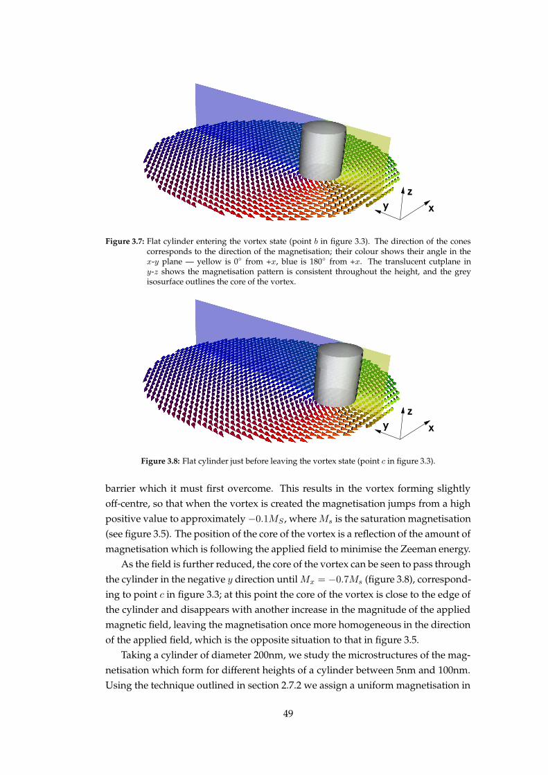
x
zy
Figure 3.7: Flat cylinder entering the vortex state (point b in figure 3.3). The direction of the conescorresponds to the direction of the magnetisation; their colour shows their angle in thex-y plane — yellow is 0◦ from +x, blue is 180◦ from +x. The translucent cutplane iny-z shows the magnetisation pattern is consistent throughout the height, and the greyisosurface outlines the core of the vortex.
x
zy
Figure 3.8: Flat cylinder just before leaving the vortex state (point c in figure 3.3).
barrier which it must first overcome. This results in the vortex forming slightlyoff-centre, so that when the vortex is created the magnetisation jumps from a highpositive value to approximately −0.1MS , where Ms is the saturation magnetisation(see figure 3.5). The position of the core of the vortex is a reflection of the amount ofmagnetisation which is following the applied field to minimise the Zeeman energy.
As the field is further reduced, the core of the vortex can be seen to pass throughthe cylinder in the negative y direction until Mx = −0.7Ms (figure 3.8), correspond-ing to point c in figure 3.3; at this point the core of the vortex is close to the edge ofthe cylinder and disappears with another increase in the magnitude of the appliedmagnetic field, leaving the magnetisation once more homogeneous in the directionof the applied field, which is the opposite situation to that in figure 3.5.
Taking a cylinder of diameter 200nm, we study the microstructures of the mag-netisation which form for different heights of a cylinder between 5nm and 100nm.Using the technique outlined in section 2.7.2 we assign a uniform magnetisation in
49

Figure 3.9: Height dependence of the remanent state in cylinders - vertical cutplanes in the xz planeof a cylinder of diameter 200nm in zero applied field are shown. The images are (left) acylinder of height 35nm, (centre) h =75nm and (right) h =85nm. The colour variationrepresents the z component of the magnetisation.
the x direction, allow the system to relax in zero applied field, and make observa-tions.
Figure 3.9 shows the flower state, clearly visible in the shorter cylinders; how-ever as the height is increased, the dipolar energy exerts a greater influence, as infigure 3.6. The dipolar energy continues to exert more and more pressure on thecylinder to abandon its flower state in favour of a vortex — at a height of 75nmthe top and bottom of the cylinder are completely dominated by the magnetostaticenergy. Increasing the height a little further from here to 80nm causes this structureto collapse and fall into the vortex state at zero field.
Figure 3.10 shows the reversal behaviour of nickel cylinders dependent on heightand diameter. As height is increased, the single domain behaviour disappears andvortex reversal behaviour occurs; the same is true as the diameter is increased.
3.5 Sphere
3.5.1 Finite differences and finite elements
Figure 3.11 depicts the hysteresis loops obtained from simulations of a nickel sphere(diameter d=200nm, K1=0). The loops in the upper left, upper right and lower leftof the figure show loops yielded with the OOMMF software, whilst the lower rightloop was computed with magpar.
For each simulation, the applied field direction was varied in θ and φ, respec-tively the azimuth and polar angle of the applied field. These are relative to theorientation of the finite difference grid, aligned with the x-, y- and z-axes.
All the loops show a similar pattern just below saturation, with small openingsin the hysteresis where the magnetisation moves from the single domain state intothe vortex state.
It is interesting to note that in the loops computed with OOMMF there is an“opening” in the hysteresis loop around Bx=0, the size of which varies with thedirection of the applied field, although it is never quite eliminated. The resultsfrom magpar do not display this characteristic.
These data show that the inner loop depends on the angles θ and φ. For thespherically symmetric system that we wish to simulate, how the coordinate system
50

60 80 100 120 140 160Diameter (nm)
20
40
60
80
Hei
ght (
nm)
single-domain statevortex/multi-domain state
Figure 3.10: Phase diagram of the remanent magnetisation state for nickel cylinders of varying heightand diameter
51

-300 -200 -100 0 100 200 300
-1
-0.5
0
0.5
1
mag
netis
atio
n M
x
-400 -200 0 200 400
-1
-0.5
0
0.5
1
-300-200-100 0 100 200 300applied field Bx (mT)
-1
-0.5
0
0.5
1
mag
netis
atio
n M
x
-600 -400 -200 0 200 400 600applied field Bx (mT)
-1
-0.5
0
0.5
1
c
d
a
b
Figure 3.11: Hysteresis loops for nickel spheres of diameter d=200nm with no magnetocrystallineanisotropy with varying applied field offsets in xy (θ) and xz (φ). The top left hysteresisloop was performed with OOMMF with applied field offsets θ=45o, φ=0o. The top rightloop (OOMMF) has θ=10o, φ=0o. The bottom left loop (OOMMF) has θ=30o, φ=18o. Thebottom right hysteresis loop was performed with magpar using an applied field offset ofθ=4o, φ=6o
52

of the simulation software is aligned relative to the direction of the applied fieldshould be irrelevant. It is therefore likely that the inner openings in the hystere-sis loops are an artefact of the finite difference simulation technique as these varysubstantially as a function of this direction.
Initially, we assume the applied field is zero and the magnetisation forms a vor-tex with the core pointing in the x direction as shown later in figure 3.15, and a verysmall field is applied in the opposite direction (i.e. −x) such that the vortex struc-ture of the magnetisation is not significantly affected. Since the overall magneticmoment of the magnetisation is finite and points in the direction of the momentsin the vortex core, it is therefore energetically favourable for the system to align thevortex core with the applied field.
In order for this to happen, the vortex core needs to turn around by 180 degrees(i.e. point in −x rather than +x. If there is no magnetocrystalline anisotropy in thesystem, the spherically symmetric sphere should allow the core to rotate round ineither θ or φ, similar to a typical Stoner-Wohlfarth particle. The spherical symmetryshould not allow the occurrence of the “inner” hysteresis loop indicated in figure3.11; this is supported by the results presented in the lower right of figure 3.11computed with the finite element code.
It is plausible therefore to assume that directions along the discretisation axis areeither favoured or avoided by the system when a finite difference grid is introducedfor symmetric geometries.
3.5.2 Reversal mechanism
A strong magnetic field applied across a nickel sphere of diameter 200nm gives ahomogeneous magnetisation. As this field is reduced the magnetisation at the sur-face of the sphere diverges as a consequence of the dipolar interactions (figure 3.12corresponding to point a in figure 3.11; also shown in figure 3.13); this behaviour issimilar to that in small cylinders.
As the field is reduced, the sphere falls into the vortex state a little above 100mT(see figure 3.14, corresponding to point b in figure 3.11), but, contrary to the cylin-der, this vortex forms around the axis of the applied field. The majority of the mag-netisation at this stage is pointing in the direction of the applied field rather thanagainst it, as the core of the vortex is aligned with the direction of the initial mag-netisation. The magnetisation around the core of the vortex is able to maintain itscircular vortex pattern and adjust its alignment with the present applied field.
At zero field, the magnetisation in the vortex core remains pointing in the di-rection of the applied field (figure 3.15, corresponding to point c in figure 3.11),however if the field is increased in the −x direction then the magnetisation in thecore is reversed (figure 3.16, point d in figure 3.11).
Further increasing the field eventually results in the vortex dissipating at around
53

z
xy
z
xy
Figure 3.12: Nickel sphere in high applied field showing spin tapering owing to demagnetising en-ergy; the left image shows a cut-plane through x and y, the right image shows a cut-planethrough x and z. This corresponds to point a in figure 3.11
180mT. This results in the magnetisation of the sample pointing entirely in the di-rection of the applied field as in figure 3.13, only in the opposite direction.
3.5.3 Size dependence
A size dependence study was performed on the diameter of nickel spheres; theresults of this can be seen in figure 3.17, showing a change in behaviour at a certaindiameter.
There is a qualitative change in the magnetisation reversal when the diameteris reduced; the hysteresis loops for spheres of diameter 50nm and 80nm are shownin figure 3.18.
The following equation (O’Handley, 1999) gives the critical radius (i.e. the radiusabove which a sphere changes from single domain behaviour to vortex behaviour)of a spherical sample of some material which has a low anisotropy value.
rn+1 =
√
9A
µ0M2s
[
ln
(
2rn
a
)
− 1
]
(3.1)
Using this equation, one can quickly converge on the critical radius for nickel byiterating equation 3.1 until rn+1 − rn = 0. The calculated critical radius of 34nmagrees well with our simulations of nickel spheres; these studies show that themagnetisation pattern of a nickel sphere of diameter 60nm (r = 30nm) reversesas a single-domain, and the magnetisation pattern when the diameter is 70nm isvortex-like.
3.6 Summary
We have studied the magnetisation reversal in nickel cylinders and spheres of thesize order 200nm. Around this size, in nickel the samples will not tend to form
54

y xz
Figure 3.13: Sphere at high applied field (point a in figure 3.11); see also figure 3.12.
y xz
Figure 3.14: Sphere immediately after entering the vortex state (point b in figure 3.11).
55

y xz
Figure 3.15: Sphere in vortex state (point c in figure 3.11).
y xz
Figure 3.16: Sphere in vortex state at a further reduced field (point d in figure 3.11).
56

40 60 80 100 120 140 160diameter (nm)
vortexsingle domain
critical radius = 34nm
Figure 3.17: Size dependence of the domain state in nickel spheres. The vertical dotted line showsthe critical radius for state transition computed with equation 3.1
-200 -100 0 100 200applied field Bx (mT)
-1
-0.5
0
0.5
1
mag
netis
atio
n M
x
-200 -100 0 100 200applied field Bx (mT)
-1
-0.5
0
0.5
1
Figure 3.18: Hysteresis loops for nickel spheres of (left) diameter 50nm and (right) diameter 80nm.The 50nm sphere reverses through the single-domain state; the 80nm sphere through thevortex state
57

domain walls as the samples are physically too small — the energy from dipolarinteraction is not great enough to counteract the domain wall energy — and neitherwill the shapes behave as single-domain states as the dipolar energy is then toogreat (Wachowiak et al., 2002).
Below a certain critical diameter, cylinders exhibit single-domain behaviour.Above this critical diameter, the cylinders enter the vortex state. In this regime,the vortex penetrates and moves to adapt Mx to Bx after the field is reversed. Inall cases, nickel cylinders cannot maintain a single-domain reversal method oncetheir height is above a critical value; we find that the vortex reversal method ispresent in all cylinders with a height greater than 60nm. The results for the simu-lated cylinders are qualitatively in agreement with work by Cowburn et al. (1999b),however these cannot be compared directly because different materials have beeninvestigated.
With the simulated spheres, vortex behaviour exists for a sufficiently large sys-tem, however the vortex penetrates at a greater applied field than that in a cylinderof comparable size. The vortex in spheres is also static with the core of the vortexpointing in the original direction of the applied field, as opposed to the vortex ap-pearing in cylindrical samples, where the core of the vortex is able to move throughthe system to compensate for a change in applied field. In cylindrical samples, thecore of the vortex is perpendicular to the direction of the applied field, i.e. it pointsout of the circular plane.
We have shown that for non-cuboidal structures, great care has be taken to en-sure that the finite difference simulation technique does not introduce artefacts thatdo not reflect the behaviour of the physical system. In subsequent chapters we haveused finite element simulations to corroborate finite difference simulation results,and varied the directions of applied field to ensure to exclude such artefacts fromour observations.
58

Chapter 4
Cones
The work described in this chapter has been submitted to Physical Review B (Board-man et al., 2005a).
4.1 Introduction
Tapered structures such as pyramids and cones are commonly used in magneticforce microscopy (Dahlberg and Proksch, 1999, Saenz et al., 1987); the phase shift in-duced by the movement of a cantilever attached to the structure can be interpretedto yield the stray field pattern of a sample (McVitie et al., 2001).
Part-conical samples of size order 1µm and above have previously been fabri-cated for bubble devices (Sanders et al., 1981). Nanolithographically defined struc-tures created through electron beam lithography (Chou, 1997, Chou et al., 1996) re-sult in arrays of tapered pillars which are geometrically conical. The coercivity ofarrays of shorter cones created with interference lithography has been previouslyinvestigated experimentally and numerically (Ross et al., 2001).
In this chapter, we study the magnetic reversal behaviour of cones systemati-cally and compute a magnetisation remanence phase diagram as a function of di-ameter and height.
4.2 Parameters
We use the material parameters for Ni80Fe20 permalloy (Js = 1.0 T, A = 1.3×10⁻¹¹
J/m, K1 = 0.0 J/m3) (Skomski and Coey, 1999) and a damping constant α of 0.25 toimprove convergence.
We perform simulations on cones where the overall diameter d of the baseranges from 10nm to 100nm, the height h between the base and the tip ranges from10nm to 100nm and the external magnetic field is applied along the x direction ofthe cone (see figure 4.1).
59

xy
z
single domain x single domain z buckle state C state out−of−plane vortex
d
h
Figure 4.1: Representation of remanent magnetisation states; the solid arrows indicate the magnetisa-tion direction, the dotted arrow shows the vortex core direction. From left to right: singledomain state in x, single domain state in +z (filled arrow) and −z (hollow arrow), bucklestate (Koltsov et al., 2000), C state and out-of-plane vortex state.
The mesh for the magpar hybrid FE/BE simulation is created using NETGEN(Schoberl, 2003). For the cone where d = 100nm and h = 100nm, the mesh contains210825 tetrahedra, with the largest element having an edge length smaller than4nm, which is below (Donahue and McMichael, 1997) the calculated exchange lengthλex =
√
2A/µ0M2s (Kronmuller and Fahnle, 2003) of 5.71nm.
The remanent magnetisation configurations using OOMMF and magpar are inagreement providing the shape is sufficiently well resolved in both cases. To ensurethis is the case with OOMMF, the cones were discretised into 8000 cells, in thelargest case the cell edge length is 5nm with a maximum adjacent cell spin angle of0.5 radians.
Starting from an initially uniform magnetisation state pointing in the +x direc-tion, we apply a magnetic field of 500mT capable of maintaining a nearly homoge-neous magnetisation and reduce this field in steps of 1mT until the magnetisationis reversed to compute the hysteresis loop. When the applied field is reduced tozero, we classify the magnetisation pattern to create the remanence phase diagram.Figure 4.1 shows schematic plots of the observed remanent states.
4.3 Results
Figure 4.2 shows the phase diagram for the remanent magnetisation states in coneswhere 10nm ≤ d ≤ 100nm and 10nm ≤ h ≤ 100nm and the applied field was orig-inally in the +x direction (see figure 4.1). Where h is less than 20nm, the remanentstate is a single domain state with the magnetisation pointing in the x direction(figure 4.1, left). If h is above 50nm and the ratio h/d is high (i.e. a tall, thin cone)then the single domain state in z is preferable due to shape anisotropy (figure 4.1,second from left). We have observed two types of single domain states in z: onewith the magnetisation pointing up towards the tip of the cone and the other withthe magnetisation pointing down towards the base. The single domain states in x
60

20 40 60 80 100diameter (nm)
20
40
60
80
100
heig
ht (
nm)
single domain in xsingle domain in zC state in xzbuckle stateout-of-plane vortex
Figure 4.2: Phase diagram of the remanent magnetisation states for cones where the applied field wasoriginally in the +x direction. The symbols represent computed points, dashed lines areguides to the eye.
61

-300 -200 -100 0 100 200 300applied field Bx (mT)
-1
-0.5
0
0.5
1
mag
netis
atio
n M
x
A
D
C
B
xz
y
EF
GH
Mx−1.0 1.0
Figure 4.3: Hysteresis loop and reversal mechanism for a cone where d = h =100nm and the appliedfield is across the diameter. Points E, F, G and H are explained in figure 4.4.
and z are in agreement with experimental data in Ross et al. (2001).For larger h and d the demagnetising energy grows and the remanent state is
the vortex state with the magnetisation in the core of the vortex pointing out of thexy plane (figure 4.1, right).
For intermediate values of h we find at large d the buckle state (figure 4.1, cen-tre), in which the overall magnetisation points in x but around the centre of the xy
plane this bends slightly upwards and downwards in z. The buckling is an indica-tion of the growing dipolar energy of the single-domain state.
At smaller d for intermediate h the remanent state is a C-shaped configuration(figure 4.1, second from right). The C state is related to the single domain state inz by the shape anisotropy driving the magnetisation to point primarily in the -zdirection. In larger diameters the magnetisation will attempt to reduce the demag-netisation energy — the bending of the magnetisation in the +x direction close tothe base of the cone shows the history of the system: prior to the field being reducedto zero the magnetisation was pointing in the +x direction.
Figure 4.3 shows the complete hysteresis loop for a cone with d=h=100nm, com-puted using magpar. When the applied field is reduced from saturating the mag-netisation in the +x direction, it forms an in-plane vortex (i.e. where the mag-netisation circulates in yz and the vortex core points in the x direction) shown at
62

point A. The same behaviour is observed for the magnetisation reversal of spheres(Boardman et al., 2005b, Eisenstein and Aharoni, 1975) of similar size. Note that thisconfiguration is not observed in the absence of an applied field and therefore thisstate is not shown in figure 4.1.
The in-plane vortex is replaced by an out-of-plane vortex (i.e. where the mag-netisation circulates in xy and the vortex core points in the z direction) shown atpoint B after overcoming an energy barrier. The core of this vortex is anchored atthe tip of the cone and compensates for the applied field by tilting the core, allowingthe majority of the magnetisation to align with the applied field, thus minimisingZeeman energy.
A further reduction of the field (point C) causes the core of the vortex to shift tothe centre of the cone. Reducing the field below zero causes the vortex to bend inthe opposite direction to point B. At Bx = 0mT the magnetisation is in the vortexstate as shown in figure 4.1 (right). Another energy barrier needs to be overcome todestroy the out-of-plane vortex, leaving the magnetisation with an in-plane vortex(point D) with the core pointing in the opposite direction to the vortex at point A.
Once the field is sufficiently high the in-plane vortex aligns into a homogeneoussaturated magnetisation in the -x direction for |Bx| ≥ 250mT.
Figure 4.4 shows specifically the magnetisation at points E, F, G and H fromfigure 4.3 to explain the subtle “kinks” in the hysteresis loop. The top row showsa magnetisation cross section along the height of the cone and the bottom row thatalong the base. The middle row is a schematic representation of the two vorticescorresponding to the cross sections above and below.
Starting at point E, the system contains two vortices: the out-of-plane vortexwith the core pointing in the +z direction introduced at point B, and the formationof an in-plane vortex with the core in the -x direction parallel to the applied field.Increasing the field in the -x direction causes the in-plane vortex to become moredominant (point F). A further increase of the applied field in the -x direction allowsthe in-plane vortex to become even more influential, moving the out-of-plane vor-tex to the edge of the sample (point G). There is a small energy barrier present toforce the out-of-plane vortex from the system; once this has been overcome onlythe in-plane vortex remains (point H).
4.4 Summary
We have simulated the magnetisation reversal in conical samples, and five separateremanent states — single-domain in x, single-domain in z, out-of-plane vortex,buckle and C-state — have been observed.
By analysing the remanent magnetisation configuration for a series of simula-tions, we have created a phase diagram showing these results. The dynamics of the
63

z
y
x
y
z
y
x
E F G H
Figure 4.4: Reversal mechanism detail for points E, F, G and H in figure 4.3. Top: yz cutplanes ofmagnetisation shaded by the x component of the magnetisation (Mx). Middle: schemat-ics indicating vortex behaviour (solid arrows for the in-plane vortex shown the in toprow, dashed arrows for the out-of-plane vortex shown in the bottom row). Bottom: xycutplanes of the magnetisation at the base of the cone.
magnetisation reversal are more complicated to classify and describe.We have investigated and presented in more detail the magnetisation reversal
of larger cones (height greater than 70nm and diameter greater than 50nm) andfind that for parts of the hysteresis loop, two coexisting vortices can be found in themagnetisation (with cores pointing in approximately perpendicular directions).
64

Chapter 5
Nanodots
The work described in this chapter has been published in two papers in the Journalof Applied Physics (Boardman et al., 2004, 2005b).
5.1 Introduction
Figure 5.1 shows an array of nanodots created using the novel “double template”method imaged using a scanning electron microscope.
Figure 5.2 shows the experimentally measured hysteresis loop for such an ar-ray of nickel nanodots (see section 5.1.1) with a bounding sphere diameter d of500nm (Zhukov, 2004) obtained through magneto-optical Kerr effect (Argyres, 1955)microscopy. The motivation here is to reveal the physics in this hysteresis loopthrough micromagnetic simulation.
Although the precise shape of the nanodot is not known, we do know the man-ufacturing method (see section 5.1.3) and from this we can derive an approximaterepresentation of the nanodot.
It is not feasible to perform a three-dimensional micromagnetic simulation of alarge array of nanodots so instead a single nanodot is modelled numerically. De-spite some inevitable dipolar interaction in the real system, particularly when thenanodots are close together, it remains of interest to investigate the magnetisationof an independent nanodot.
5.1.1 What is a nanodot?
We define a nanodot to be a magnetic sample with a physical edge size lx of lessthan 1µm and “short” in geometry, i.e. lz ≤ 0.5lx. Arrays of nanodots are strongcandidates for use in patterned media, as the consistency of shape from one nan-odot to the next promotes predictable behaviour; one nanodot will behave in thesame way to another nanodot, in contrast to irregular grains where clusters ofgrains are required to reduce the effects of this irregularity.
65

Figure 5.1: Scanning electron microscope image of a droplet array
5.1.2 Lithography
There are several different ways of creating nanodots. Lithographic methods suchas those used by Cowburn et al. (1999a), Li et al. (2002) and discussed in chapter 3,although successful, are limited in the grain size they can produce; in photolithog-raphy the wavelength of light used in the fabrication process effectively limits thedot size to those above 0.4µm, and electron beam lithography is still a prohibitivelyexpensive process.
5.1.3 Self-assembly
Self-assembly methods (Denkov et al., 1993) appear to be a cost-effective way tocreate templates, from which an array of structures as shown in figure 5.1 can beformed (Ghanem et al., 2004, Zhukov et al., 2003). These structures are the motiva-tion behind this chapter. One particular method of chemical self-assembly involvesthe formation of templates through the evaporation of an aqueous suspension ofpolystyrene latex spheres (Bartlett et al., 2002, 2003a), initiating the self-assembly.Figure 5.3 shows this process schematically.
Using these templates, it is possible to create magnetic structures from sizes of50nm to 1000nm by filling the spaces between the close-packed spheres with some
66

-200 -100 0 100applied field Bx (mT)
-0.5
0
0.5
1
mag
netis
atio
n M
x
Figure 5.2: Normalised MOKE measurements for a nickel dot array of diameter 500nm
d
water latex spheres
substrate
non−magnetic material
holes
h
magnetic material
Figure 5.3: The double-template self-assembly technique. First, an aqueous suspension of latexspheres (top left) of diameter d is poured onto a substrate. As the water evaporates,the latex spheres are attracted to each other (top centre), forming a regular close-packedstructure. This template can be filled with a non-magnetic material (top right) and thelatex spheres etched away (bottom left). The resulting gaps can be filled with a magneticmaterial to a varying height h (bottom right) to form arrays of connected or disconnectedpart-spherical nanodots.
67

2/7d
1/7d
dz
x
Figure 5.4: A typical nanodot “droplet” geometry arranged in a hexagonal lattice (artist’s impressionon the left) and a schematic of the droplet (right)
material through electrochemical deposition. By etching away the polystyrenespheres, another template is formed. This template can then be filled with magneticmaterial, and by varying the fill amount of the resulting spherical holes, connectedor disconnected arrays of dots can be formed. This is known as the double-templateself-assembly method.
The resulting structures have several applications, such as photonic materi-als (Bogomolov et al., 1997, Vlasov et al., 2001), microchip reactors (Gau et al., 1999)and biosensors (Velev and Kaler, 1999). The application in which we are interestedfor this work pertains to magnetism.
We present here the results for two types of nanodot geometry — part-sphereand “droplet”. The droplet geometry can be considered to be a part-sphere with arounded upper; this is described in more detail in section 5.5.
5.2 Half-sphere
We wish to simulate a half-sphere so we can see what effect the rounded upperdome (which can be seen in figure 5.1) has on the results; these can then be com-pared to “droplet” systems (section 5.5) which reflect the shape in figure 5.1. Thehalf-sphere nanodot we simulate here is isotropic nickel (Ms = 493380 A/m, A =
8.5 × 10⁻¹² J/m, K1 = 0 J), with a diameter of 200nm. We use OOMMF to simulatethis geometry with a finite difference cubic cell of edge length 5nm.
5.2.1 Results
Applying a sufficiently large magnetic field across the circular plane of a half-sphere results in an initially homogeneous magnetisation pattern, and as with thesphere in section 3.5, a slight deviation at the surface resulting from the demagnetis-ing field. This corresponds to point a in figure 5.5; the homogeneous magnetisation
68

-400 -200 0 200 400Applied field Bx (mT)
-1
-0.5
0
0.5
1
Nor
mal
ised
mag
netis
atio
n M
x
a
b
c
Figure 5.5: Hysteresis loop for a nickel half-sphere of diameter 200nm
is illustrated in figure 5.6.Reducing the field further causes the nucleation of a vortex at around 30mT,
resulting in the magnetisation drop immediately following point a in figure 5.5.The vortex core moves in the −y direction while the field is reduced further
(point c in figure 5.5; illustrated in figure 5.8), until the vortex leaves the systemand a homogeneous magnetisation in the −x direction is established.
5.2.2 Discussion
Although hysteretically this exhibits a qualitative similarity with the sphere (fig-ure 3.11) insofar as their possession of two minor loops, the magnetic microstruc-ture is more reminiscent of the flat cylinder in that the vortex nucleates out of theplane and moves through the geometry in the same fashion as the flat cylinder (fig-ures 3.3 to 3.8), however the vortex appears prior to the applied field being reducedbelow zero.
Figure 5.7 illustrates that at zero field the direction of the vortex core is perpen-dicular to and in the centre of the xy plane; see point b in figure 5.5. For isolatedhalf-spheres we always find the magnetisation in the core of the vortex to point“down” (i.e. towards the spherical surface). We attribute this to the asymmetry ofthe half-sphere in the z direction.
69

xzy
Figure 5.6: Half-sphere at high applied field (point a in figure 5.5)
Figure 5.7: Half-sphere in vortex state in zero applied field (point b in figure 5.5). Axes are the sameas those in figure 5.6
70

Figure 5.8: Half-sphere in late vortex state (point c in figure 5.5). Axes are the same as those in fig-ure 5.6
5.3 Part-spherical nanodots
We have seen above that the magnetisation reversal in the half-sphere occurs viavortex nucleation similar to the mechanism in the flat cylinder shown in section 3.4.We have shown in section 3.5 that a full sphere reverses via a different mechanism.From this it can be concluded that for some height h > d/2 of a part-sphere atransition between the two reversal mechanisms takes place.
These results are also relevant to the experimentally manufactured nanodotsbecause the amount of material that is deposited through the self-assembly methoddescribed in section 5.1.3 can be varied to grow spheres of heights h ≤ d.
We calculate numerically the magnetisation reversal of soft part-spherical par-ticles. The observed reversal mechanisms range from single domain reversal atsmall radii, to vortex movement in shallow systems at larger radii and vortex corereversal at larger heights as observed in spheres.
In this section we study the behaviour of the new class of part-spherical struc-tures and compute a magnetic reversal phase diagram as a function of diameterand height.
5.3.1 Parameters
Geometrically we consider the part-spheres to have one flat surface when h < d; inthe case h = 0.5d the geometry will resemble the half-sphere from section 5.2.
71

12.5 25 37.5 50 62.5 75 87.5 100 112.5 125bounding sphere diameter d (nm)
0.2
0.4
0.6
0.8
1
heig
ht (
h/d)
in-plane vortexperpendicular vortexsingle domain
Figure 5.9: Phase diagram of reversal mechanisms for Ni50Fe50 permalloy part-spheres. The dottedand dashed lines are guides to the eye indicating reversal mechanism boundaries
We perform the phase diagram studies using the material parameters forNi50Fe50 permalloy (Ms = 1.11×10⁶ A/m, A = 5.85×10⁻¹² J/m, K1 = 0 J/m3, seealso appendix C) and a damping constant α of 0.25 to improve convergence.
5.3.2 Results
Figure 5.9 shows a phase diagram of remanent magnetisation states for systemssimulated with magpar where the height h increases from 1/8d to d in 1/8d stepsand d varies between 12.5nm and 125nm.
We observe three distinct reversal mechanisms. Taking d=50nm, for h/d ≤ 0.375
the reversal is coherent; all the magnetic moments remain aligned and rotate ho-mogeneously. Between h/d = 0.5 and h/d = 0.875 an out-of-plane vortex formswith a core perpendicular to the applied field after some initial energy barrier isovercome and this can freely move around the inside of the part-sphere with theapplied field. This is similar to the behaviour seen in cylindrical particles shownin figures 3.3 to 3.8 and in other works (Boardman et al., 2004, Cowburn et al., 1999b,Ha et al., 2003, Li et al., 2002). We will now discuss the reversal mechanism in moredetail.
Figure 5.10 shows the perpendicular vortex reversal behaviour. Point A showsthe homogeneously aligned state at high applied field, though there is a small C-
72

-200 -100 0 100 200applied field Bx (mT)
-1
-0.5
0
0.5
1
mag
netis
atio
n M
x
Mx
xy
z
AB
C
D
E
Figure 5.10: Reversal mechanism for d=50nm, h=0.5d
state-like shift in the x-z direction at the extremities in order to minimise dipolarenergy. At point B there is a shift into an S-like state in the x-y direction, wherethe magnetic moments at the edges of the half-sphere persist in the applied fielddirection while the moments towards the centre are aligned a few degrees awayfrom the x direction into the y direction. Reducing the field further overcomesan energy barrier and a perpendicular (i.e. the core of the vortex points in the z
direction) vortex is formed. Point C shows the remanent state of the half-spherewith this vortex in the centre; the net magnetisation in the x direction is now zero.Point D shows the effects of a continued field reduction; the vortex has shiftedfurther into the y direction appropriate for allowing the majority of the magneticmoments to point in the negative x direction. Finally, at point E the external field isnow sufficiently low to remove the vortex from the system, and a homogeneouslyaligned state remains.
Figure 5.11 shows the reversal mechanism with an in-plane vortex for a sphere(i.e. h/d = 1.0). Although the size and material differ from the sphere in section 3.5,there is a qualitative similarity we will review. Point A shows a homogeneousalignment of the magnetic moments in the x direction, which persists until point B,where the field has been lowered enough to overcome the energy barrier and allowan in-plane (i.e. where the core points in the x direction) vortex to form; this alsoallows the majority of the magnetisation to continue pointing in the x direction.
73
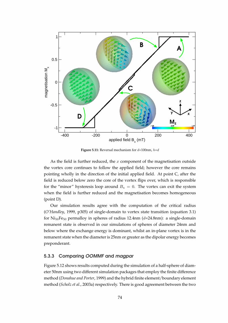
-400 -200 0 200 400applied field Bx (mT)
-1
-0.5
0
0.5
1
mag
netis
atio
n M
x
z
y x
zM
AB
C
D
Figure 5.11: Reversal mechanism for d=100nm, h=d
As the field is further reduced, the x component of the magnetisation outsidethe vortex core continues to follow the applied field; however the core remainspointing wholly in the direction of the initial applied field. At point C, after thefield is reduced below zero the core of the vortex flips over, which is responsiblefor the “minor” hysteresis loop around Bx = 0. The vortex can exit the systemwhen the field is further reduced and the magnetisation becomes homogeneous(point D).
Our simulation results agree with the computation of the critical radius(O’Handley, 1999, p305) of single-domain to vortex state transition (equation 3.1)for Ni50Fe50 permalloy in spheres of radius 12.4nm (d=24.8nm): a single-domainremanent state is observed in our simulations of spheres of diameter 24nm andbelow where the exchange energy is dominant, whilst an in-plane vortex is in theremanent state when the diameter is 25nm or greater as the dipolar energy becomespreponderant.
5.3.3 Comparing OOMMF and magpar
Figure 5.12 shows results computed during the simulation of a half-sphere of diam-eter 50nm using two different simulation packages that employ the finite differencemethod (Donahue and Porter, 1999) and the hybrid finite element/boundary elementmethod (Scholz et al., 2003a) respectively. There is good agreement between the two
74

-200 -100 0 100 200applied field Bx (mT)
-1
-0.5
0
0.5
1
mag
netis
atio
n M
x
finite differencefinite element/boundary element
Figure 5.12: Hysteresis loops for a d=50nm half-sphere obtained with (solid line) OOMMF (finitedifference method) and (dashed line) magpar (finite element/boundary element method)
packages.The results obtained from both OOMMF (FD method) and magpar (hybrid FE/BE
method) display an energy barrier which is overcome when Bx is below 50mT. Ad-ditionally, reversible behaviour around Bx = 0 is present in both cases.
The slight aberration in the hysteresis loop for the hybrid FE/BE case is causedby a slight shift in the magnetisation towards the centre of the sample (figure 5.10,point B), present in the simulation as a result of the improved shape resolution overthe FD case.
5.4 Multiple vortex states
As the diameter of a part-spherical geometry is increased, further characteristicsare observed which resemble those of the full sphere.
Figure 5.13 shows the hysteresis loop for an isotropic nickel half-sphere of di-ameter 350nm. This hysteresis loop shares some similarity with that of a smallerhalf-spherical system, such as that in figure 5.10 — it has zero remanence and thereare openings in the hysteresis loop. The characteristic difference between the twoloops is there are two energy barriers: the first occurs when Bx is around 100mT,followed by another when Bx is approximately 70mT, corresponding to the kink in
75

-200 -100 0 100 200applied field Bx (mT)
-1
-0.5
0
0.5
1
mag
netis
atio
n M
x
Figure 5.13: Hysteresis loop for an isotropic nickel half-sphere of diameter 350nm. Two energy barri-ers can be seen: one at ≈100mT and another at ≈70mT. The first indicates the transitionfrom the single-domain state to the in-plane vortex state, the second the transition fromthe in-plane vortex state to the perpendicular vortex state.
the curve at 60mT in figure 5.10.Figure 5.14 reveals the magnetic microstructures in this model. The image on
the left shows the magnetisation when Bx is 80mT. An in-plane vortex has formedand the magnetisation circulates in the yz plane, with the core of the vortex point-ing in the x direction with the applied field. The image on the right shows themagnetisation after Bx has been reduced to 65mT. The in-plane vortex has been re-placed by a perpendicular vortex: the magnetisation now circulates in the xy planewith the core of the vortex pointing in the z direction. The core of the vortex isoff-centre to allow the majority of the magnetisation to point in the direction of theapplied field.
Figure 5.15 shows the hysteresis loop when the diameter of the nickel half-sphere is increased to 750nm. Qualitatively, the same behaviour is observed aswhen the half-sphere diameter is 350nm. Point A shows the fully-saturated mag-netisation at a high applied field in the +x direction. When this is reduced to over-come the first energy barrier (point B) then the in-plane vortex forms, with the coreof the vortex pointing in the direction of the applied field. As the field is reduced toimmediately prior to the second energy barrier at around 75mT (point C), the mag-netisation around the core of the vortex deviates further away from the x direction
76

yx
z
Figure 5.14: Two vortex states in an isotropic nickel half-sphere of diameter 350nm. The images showvector cut-planes of magnetisation in the y-z direction — applied field was in the x direc-tion. The in-plane vortex (left) is clearly visible at Bx ≈80mT. The perpendicular vortex(right) is in a field of ≈65mT, and is off-centre to compensate for the applied field.
to minimise dipolar energy.Point D shows the magnetisation immediately after the second energy barrier
has been overcome. The in-plane vortex has disappeared to be replaced by a per-pendicular vortex, with the core pointing in the z direction. The majority of themagnetisation remains in the direction of the applied field. Reducing the field tozero (point E) sees the vortex core move across the sample in the y direction, caus-ing the average Mx to be zero. Increasing the applied field in the opposite direction(−x) causes the vortex core to move further along the y direction (point F) allowingthe majority of the magnetisation to point in the −x direction, similar to point D.
Increasing the field further in the −x direction overcomes another energy bar-rier present around -125mT (point G), causing the perpendicular vortex to disap-pear and an in-plane vortex with the core pointing in −x to form, which disappearswhen the applied field is increased to -140mT (point H).
5.5 “Droplet” nanodots
5.5.1 Parameters
In this instance, the geometry of the nanodot is similar to that of a “droplet”; weconsider the shape to be split into two parts — the lower part follows a “boundingsphere” to some fraction, at which point it is cut off to form a part-sphere. Thisis then provided with an ellipsoidal top, giving the geometry a dome-topped ap-pearance, which can be seen more clearly in figure 5.4, in order to approximate theexperimentally grown droplets (figure 5.1) as well as possible..
For these simulations, we define the height of the geometry thus (as figure 5.4,
77

-200 -100 0 100 200applied field Bx (mT)
-1
-0.5
0
0.5
1m
agne
tisat
ion
Mx
ab
c
d
e
f
g
h
y
z
Figure 5.15: Hysteresis loop for isotropic nickel half-sphere of diameter 750nm simulated with mag-par. The coloured sections of the smaller images represent the magnetisation in the xdirection
x component of magnetisation
−1 1
+x applied field zero applied field −x applied field
z
y
Figure 5.16: Vortex “pinning” in a part-sphere of height 0.75d. After entering an in-plane vortex state(left), the upper part of the vortex core is situated about the centre of the xy plane whilethe lower part is towards +y. When the field is reduced to zero (centre), the upper andlower parts of the vortex core are around the centre of the xy plane. If a negative fieldis then applied (right), then the lower part of the vortex core moves towards −y, but theupper part remains at the centre of xy.
78

-100 -50 0 50 100applied field B
x (mT)
-1
-0.5
0
0.5
1
norm
alis
ed m
agne
tisat
ion
Mx
A
C
D
B
Figure 5.17: The hysteresis loop for the 140nm droplet with inset x-y cut-planes showing vortex prop-agation
right):
lz(s) = 2/7d (5.1)
lz(e) = 1/7d (5.2)
∴ lz = 3/7d (5.3)
< 1/2d (5.4)
where lz(s) is the part which follows the outline of some bounding sphere of diam-eter d, and lz(e) is the upper ellipsoidal dome part. These parameters most closelyreflect the geometry of droplets resulting from the partial filling of templates withspherical voids. We study the results of simulations performed on such nanodotswith d between 50nm and 500nm.
5.5.2 Reversal mechanism
Figure 5.17 shows the hysteresis loop for a droplet with bounding sphere diameterd = 140nm. From an initially homogeneous magnetisation brought about throughthe application of a saturating magnetic field in the x direction, a slight taperingeffect appears at the surface as this field is reduced owing to long-range dipolar
79

-400 -200 0 200 400Applied field Bx (mT)
Mag
netis
atio
n
140nm350nm500nm
-100 -50 0 50 100
-1
0
1
Figure 5.18: Hysteresis loops for droplets of bounding sphere diameter 140nm, 350nm and 500nm;note that the loops are offset in the y direction for clarity. Inset is the hysteresis loop fora droplet of bounding sphere diameter 50nm.
80

interactions (see figure 5.17, point A).Further reduction of the applied field causes the dipolar energy to become more
dominant. At slightly above zero field this causes the formation of a vortex slightlyaway from the sample centre (see figure 5.17, point B), the direction of which allowsthe overall magnetisation direction to remain in that of the applied field. The vortexmoves closer to the centre of the sample as the field tends towards zero, and whenthere is no applied field, the Zeeman energy term is also zero and the vortex movesto the centre.
The net magnetisation Mx of the sample at this point is now zero (see figure 5.17,point C). Reducing the field further (i.e. increased in the opposite direction) shiftsthe vortex further across the sample (see figure 5.17, point D), until the Zeemanenergy term influences the magnetisation more than the other energy terms and themagnetisation of the sample becomes homogeneous in the direction of the appliedfield.
It is interesting to note that if the height lz(s) from equation 5.1 is increased toaround 0.5d, the reversal mechanism is slightly different. Although the magneti-sation falls into the vortex state, only the lower half of the vortex moves throughthe system; the upper half is ‘pinned’ to the centre of the ellipsoidal part during theentire reversal in a similar fashion to the three-quarter sphere in figure 5.16. Thisgives the vortex a pendulum-like movement throughout the system. Indeed, im-mediately after nucleation, the vortex is almost flat across the droplet in the planeof the applied field in a similar way to the sphere in section 3.5.
5.5.3 Size dependence
We have varied the diameter d of the droplet from 50nm to 500nm and computeda hysteresis loop for every d in steps of 10nm. We find two different regimes. Fig-ure 5.19 reflects the size dependence of the coercive field for these droplets.
When d < 140nm, the magnetisation reversal mechanism is single-domain (seefigure 5.21, left and centre). When d ≥ 140nm, the magnetisation reverses throughthe vortex state (see figure 5.17 and figure 5.21, right).
The relatively consistent coercivity of 5mT between 60nm and 130nm in fig-ure 5.19 is a result of a coherent rotation reversal process, unlike that shown bydots smaller than 60nm. The hysteresis loops at 60nm ≤ d ≤ 130nm are substan-tially less “square” than those shown with sub-60nm bounding sphere sizes andbear a resemblance to the loops from 140nm and greater droplets, as indicated bythe centre loop (d=90nm)in figure 5.21.
Above 140nm the coercivity of the droplets is zero. For droplets of greater sizethe hysteresis characteristics are similar, although as the size is increased the rever-sal takes place over an increasingly large applied field, and the smaller loops at thetop and bottom of the hysteresis graph become more rounded (see figure 5.18).
81

100 200 300 400 500Droplet bounding sphere diameter (nm)
0
5
10
15
20
25C
oerc
ive
field
Bc (
mT
)
Figure 5.19: Size dependence of coercive field in droplet nanodots. An error of ±1mT is present asthis is the applied field step size. Where Bc > 0mT, the remanent state is single domain,where Bc = 0mT there is a vortex remanent state.
-200 -100 0 100 200applied field Bx (mT)
-1
-0.5
0
0.5
1
mag
netis
atio
n M
x
-200 -100 0 100 200applied field Bx (mT)
-1
-0.5
0
0.5
1
mag
netis
atio
n M
x
Figure 5.20: Two hysteresis curves for nickel nanodots with bounding sphere diameter of 500nm. Thehysteresis loop on the left shows results obtained from experiment. The right-hand loopshows the results of the numerical modelling.
82

-200 0 200Applied field Bx (mT)
-1
0
1
Nor
mal
ised
mag
netis
atio
n M
x
-200 0 200Applied field Bx (mT)
-200 0 200Applied field Bx (mT)
Figure 5.21: Hysteresis loops for droplet nanodots of (from left to right) bounding sphere diameter dof 30nm, 90nm and 140nm
There is a good agreement between the experimental hysteresis curve measuredacross a nickel nanodot of bounding sphere diameter 500nm (figure 5.20, left) andthe results of the numerical simulation for the droplet of the same bounding spherediameter (figure 5.20, right).
5.6 Applying an out-of-plane external field
By adjusting the direction of the applied field such that it is now along the shortaxis of the droplet, or out-of-plane, rather than across the symmetry plane we canperform further studies on the droplet nanodot.
Figure 5.22 demonstrates a typical hysteresis loop obtained from these simula-tions and also the associated reversal mechanism. The vignette images along thehysteresis loop show a cut-plane of the magnetisation in the xz plane, z being theshort axis and that of the applied field. Initially, a high external magnetic field isapplied such that the magnetisation becomes homogeneous in +z (point A), thenthis field is gradually lowered until it is sufficiently high in the opposite direction(−z) to maintain a homogeneous magnetisation in this direction.
As the field is reduced, the system falls into the out-of-plane vortex state withno apparent energy barrier to overcome (point B), with the core pointing in the di-rection of the initial applied field (point C). Further reduction of the applied fieldresults in the magnetisation surrounding the core pointing more towards the di-rection of the applied field, so that when the applied field is < 0mT the overallmagnetisation is in −z (point D). The core, however, remains pointing in +z untilaround −50mT, at which point the core flips causing the small jump in magnetisa-tion around this point (point E).
Finally, once the magnetisation is sufficiently large in −z, the vortex disappearscompletely and the magnetisation is homogeneous in −z (point F).
Figure 5.23 shows the size dependence of the droplets when the applied fieldis out of the plane. The coercive field of the droplets decreases as the bounding
83

-400 -200 0 200 400applied field Bz (mT)
-1
-0.5
0
0.5
1
mag
netis
atio
n M
z
AB
C
DE
F
Figure 5.22: Reversal mechanism of a nickel droplet of bounding sphere diameter 200nm in a per-pendicular applied field
84

50 60 70 80 90 100bounding sphere radius (nm)
10
20
30
40
50co
erci
vity
Bc (
mT
)
100 120 140 160 180 200bounding sphere diameter (nm)
Figure 5.23: Size dependence of the out-of-plane coercive field in droplet nanodots.
sphere radius is increased, with the rate of coercivity reduction decreasing as theradius is further increased.
Figure 5.24 places the coercive field size dependence of the droplets where theinitial applied field is out of the plane into context by comparing this to the coer-civity of the same droplets when the original applied field is in the plane. It is clearfrom these results that applying the field across the short out-of-plane axis of thedroplets increases the coercivity significantly; for a coercive field of 20mT a dropletof bounding sphere diameter of around 25nm is sufficient with an in-plane appliedfield, however with an out-of-plane field a bounding sphere diameter of ≈160nmis required.
5.7 Summary
We have simulated the magnetisation reversal in part-spherical and droplet nan-odots. In droplet nanodots, we observe two different mechanisms for this reversal— the single-domain state and the vortex state.
If the overall size of the droplet system is increased then we notice a distincttransition from the single domain state to the vortex state, which we identify for
85

0 50 100 150 200bounding sphere diameter (nm)
0
10
20
30
40
coer
civi
ty B
c (m
T)
Bx vs. Mx
Bz vs. Mz
Figure 5.24: Size dependence of the out-of-plane (see figure 5.19) and in-plane coercive field (see fig-ure 5.23 in droplet nanodots. Mx is the in-plane magnetisation, Bx the in-plane appliedfield, Mz the out-of-plane magnetisation and Bz the out-of-plane applied field
86

isotropic nickel (see appendix C) as being at a droplet bounding sphere diameter of140nm (physical droplet diameter in this instance is around 90% of the boundingsphere diameter, approximately 126nm, and h =3/7d = 60nm). This change occursat a smaller diameter than for thin (h ≤ 30nm) circular nanodots (see figure 3.10).
The “soft” vortex behaviour — i.e. the vortex will readily adjust its position toaccommodate a change in applied field — observed in the large droplets is a usefulcharacteristic in sensor applications; smaller droplets have the square hysteresisloops desirable for data storage.
In part-spherical particles, three separate remanent states — single-domain,out-of-plane vortex and in-plane vortex — have been observed.
As the diameter of the part-spherical particle decreases, a larger h/d is necessaryfor a vortex to form. As h is increased, the magnetisation is more likely to form avortex. Below a critical radius of 12.4nm for Ni50Fe50, all h/d values will result in asingle-domain remanent state.
The hysteresis loops observed experimentally agree well with the numericalresults from the simulation.
We observe good agreement between the finite difference method in OOMMFand the hybrid finite element/boundary element model in magpar.
87

Chapter 6
Antidots
Parts of this work have been submitted for publication as Zhukov et al. (2004a)and Zhukov et al. (2004b). Experimental measurements were obtained by Dr. Alexan-der Zhukov of the School of Physics and Astronomy (University of Southampton)and the Monte Carlo simulations performed by Dr. Hans Fangohr of the School ofEngineering Sciences (University of Southampton).
6.1 Introduction
Lithographic techniques have allowed researchers to create ordered structures onthe sub-micron scale (Cowburn et al., 1997, Fruchart et al., 1999, Hehn et al., 1996,Martın et al., 2003, Van Roy et al., 1993), either as well-formed small magnetic ele-ments such as the cylindrical and spherical objects described in chapters 3 and 5or as regular arrays of holes in magnetic films. Antidots are the ‘opposite’ of thenanodots discussed in the previous chapter. If one creates a hole in a thin sam-ple, the hole can be considered to be an antidot. Lithographic techniques generallyyield cylindrical holes, but emerging self-assembly techniques (Bartlett et al., 2002)promise a wider range of shapes.
Figure 6.1 shows the single-template self-assembly technique. Electrochemicaldeposition can be used to create nanoscale magnetic materials by creating an or-dered template from polystyrene latex spheres of size order 50nm ≤ d ≤ 1000nm(Bartlett et al., 2003b, Xu et al., 2000). Initially, an aqueous solution of monodisperselatex spheres is deposited on a glass substrate. On this substrate sputtered bufferlayers of chromium and gold have been deposited, with thicknesses of 10nm and200nm respectively.
Over a period of between three and five days the evaporation of the water leadsto the formation of the template: the combination of the electrostatic repulsion be-tween the latex spheres and the attractive capillary forces provided by the evapo-ration of the water produces a well-ordered close-packed structure (Bartlett et al.,2002, 2000, 2003b).
88

h
d
water latex spheres
substrate
magnetic material
Figure 6.1: The single-template self-assembly technique. Latex spheres of diameter d are poured onto a substrate (left). As the water evaporates, the latex spheres become close-packed,forming a template (centre) which can then be filled with a magnetic material from thesubstrate upwards to a height h (right).
Using electrodeposition from the gold layer, the electrodeposited material fillsthe spaces between the latex spheres, using the spheres as a mould. By dissolvingthe latex spheres in toluene, 3D antidot arrays with spherical holes are formed.
Different thicknesses of antidot arrays can be formed by adjusting the chargeduring the electrodeposition process, while the period of the antidots is controlledby altering the diameter of the latex spheres.
Figure 6.2 shows a scanning electron microscope image of an antidot array cre-ated through the self-assembly template method, and demonstrates the regularstructure formed with this process.
Figure 6.3 shows the experimentally-measured coercivity of Ni50Fe50 antidotarrays with a diameter d of 550nm when the external field is applied in-plane. Thecoercivity oscillates as a function of height (thickness) h. When the height of thefilm is close to the sphere centres, the coercivity reaches a local maximum. Thisoscillatory behaviour is what we wish to understand and explain in this chapter.
6.1.1 The hexagonal lattice
For a hexagonal lattice with base vectors:
a1 = ax (6.1)
a2 =1
2ax +
√3
2ay (6.2)
a3 =
√
8
3az (6.3)
the lattice points are:
P = n1a1 + n2a2 + n3a3 (6.4)
(n1, n2, n3) ∈ � 3 (6.5)
89

Figure 6.2: Scanning electron microscope image of an antidot array created by the self-assembly tem-plate method. The image on the left shows the top of the array; the right-hand imageshows the honeycomb-like structure at the edge of the sample
coer
cive
fiel
d (m
T)
0
10
2
4
6
8
12
14
1.0 2.0 2.5 3.00.0 0.5 1.5h / d
Figure 6.3: Experimentally observed coercivity oscillation in Ni50Fe50 antidot arrays of d=550nmagainst the height (thickness) h of the film. The dashed lines indicate the positions ofsphere centres for each layer in the close-packed structure. The coercivity shows maximaclose to the sphere centres. The solid line is a guide to the eye
90

Figure 6.4: Two layers of spheres packed cubically (left) and hexagonally (right)
Shown in figure 6.4 on the right is a hexagonal structure which exhibits this prop-erty. However, one should note that there are two ways of packing this layer asthere are two positions in which the first sphere can be placed. The two structuresare called hexagonal close-packed and face-centred cubic. The hexagonal close-packedstructure, or hcp, has the third layer in c having the same x and y coordinates asthe first layer, the second layer has the same x and y coordinates as the fourth layer(ABABAB. . . ) and so on (Kittel, 1996). The face-centred cubic structure has an alter-native arrangement of spheres in the third layer where the spheres share the samex coordinate with the first layer but have different y coordinates (ABCABC. . . ).Although this arrangement appears at the outset to be hexagonal, by rotating itsprimitive cell the vectors can be shown to be a variant of a cubic lattice.
6.2 Parameters of the antidot system
Since three-dimensional arrays of objects become rapidly impractical to simulateeven across modern supercomputing clusters, a feasibility study was conducted toassess the limits of the available hardware when computing the hysteresis loops forthese systems.
A set of different self-assembled experimental samples were prepared fromnickel, iron, cobalt and Ni50Fe50 permalloy from spheres sized 20nm ≤ d ≤ 1000nm.For the initial micromagnetic study we chose to model the nickel sample. Nickelhas a relatively large exchange length (λex ≈ 7.5nm) when compared to Ni50Fe50
permalloy (λex ≈ 2.75nm), allowing for physically larger systems to be computedwithin a simulation domain of a comparable discrete cell count.
For the simulations, the parameters for amorphous nickel were selected (Ms =
4.93×10⁵ A/m, A = 8.5×10⁻¹² J/m, K1 = 0 J/m3) and to improve convergence adamping constant α of 0.25 was chosen.
91

Figure 6.5: 600x600x150nm cut of simple cubic nickel antispheres in zero applied field. The colouringrepresents the angle between x and y in radians; the lower left inset shows an x-y cut-plane through the centre of the sample, the lower right shows a cut-plane through a lowerpart of the same sample
6.3 Three-dimensional model
A cubic arrangement of antispheres of radius 150nm cut from a sample of nickel ofdimensions 600nm × 600nm × 150nm was prepared and the remanent magnetisa-tion computed for this system with a finite difference cell edge length of 5nm. Theseparticular dimensions were chosen as they represent the largest system which canbe simulated in a timely fashion.
The magnetic microstructures which this system creates in zero applied fieldafter being relaxed from an initially homogeneous state in the x direction can beseen in figure 6.5. Unfortunately it would appear that the effect of the edges inthis system overwhelmingly influences the microstructure, so such a small sampledoes not provide a particularly useful insight into an effectively infinite array ofantispheres. In particular, the relatively thin physical walls in the z direction whichexist in this arrangement apparently act as pinning centres of sorts; since it is dif-ficult for the system to influence the middle of these walls, the system must havea significantly large external magnetic field applied to it for these spins to reverse
92
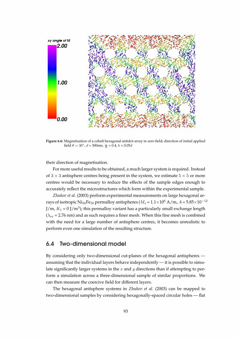
Figure 6.6: Magnetisation of a cobalt hexagonal antidot array in zero field; direction of initial appliedfield θ = 30o, d = 300nm, r
R= 0.4, h = 0.05d
their direction of magnetisation.For more useful results to be obtained, a much larger system is required. Instead
of 3 × 3 antisphere centres being present in the system, we estimate 5 × 5 or morecentres would be necessary to reduce the effects of the sample edges enough toaccurately reflect the microstructures which form within the experimental sample.
Zhukov et al. (2003) perform experimental measurements on large hexagonal ar-rays of isotropic Ni50Fe50 permalloy antispheres (Ms = 1.1×10⁶ A/m, A = 5.85×10⁻¹²
J/m, K1 = 0 J/m3); this permalloy variant has a particularly small exchange length(λex = 2.76 nm) and as such requires a finer mesh. When this fine mesh is combinedwith the need for a large number of antisphere centres, it becomes unrealistic toperform even one simulation of the resulting structure.
6.4 Two-dimensional model
By considering only two-dimensional cut-planes of the hexagonal antispheres —assuming that the individual layers behave independently — it is possible to simu-late significantly larger systems in the x and y directions than if attempting to per-form a simulation across a three-dimensional sample of similar proportions. Wecan then measure the coercive field for different layers.
The hexagonal antisphere systems in Zhukov et al. (2003) can be mapped totwo-dimensional samples by considering hexagonally-spaced circular holes — flat
93

-200 -100 0 100 200applied field B (mT)
-1
-0.5
0
0.5
1
mag
netis
atio
n M
x
Figure 6.7: Hysteresis loop for a 2d array of hexagonally arranged permalloy antidots (d = 100nm,hole radius to spacing period radius ratio r/R = 0.4) in an in-plane applied field offset 30degrees from the x direction
94

antidots — in a thin film. By varying the ratio of hole radius r to spacing radius R
the surface of the antisphere geometry at different heights can be modelled reason-ably accurately. Since larger systems can be simulated, the influence of the sampleedges detailed in section 6.3 is substantially reduced (figure 6.6).
6.5 Stray field measurement
The development of the scanning tunnelling microscope (STM) allowed scientiststo determine the electronic topography of a sample with a resolution down to afew angstroms (Binnig and Rohrer, 1985, Binnig et al., 1982, 1983). The atomic forcemicroscope (AFM) is a further development of the STM which exploits the defor-mation of a spring attached to a cantilever to allow the measurement of the forceexerted on the sharp AFM tip (Binnig et al., 1986).
To characterise the magnetic properties of a sample, the standard diamond tipof the AFM is replaced by a ferromagnetic tip (Rugar et al., 1990, Saenz et al., 1987)allowing the observation of magnetic domain structures by measuring the forcegradient exerted on the tip by the stray field as a function of the position — a tech-nique known as magnetic force microscopy (MFM) . Rather than the tip followingthe surface contours of the sample as in STM, the MFM operates with the tip at afixed z point in space.
To assess the appropriateness of the two-dimensional approximation above, wecompute the stray field and compare this to the experimental images providedthrough magnetic force microscopy.
The tip of an MFM is magnetic and we assume that it is a dipole d. In theabsence of knowledge of the precise magnetisation of the tip, this is the simplestapproach possible (Barthelmeß et al., 2003). The signal which the MFM records isproportional to the gradient of the demagnetising field Hde.
6.5.1 Numerical calculation of the stray field
We compute the stray field from our simulation data as it would be read from amagnetic force microscope by simulating several layers of “empty space” abovethe sample and measuring the demagnetising field. This has the advantage thatthe efficient OOMMF algorithm for the computation of the demagnetising field canbe used. However, we need to compute the second derivative numerically (usingcentral differences):
∂2f
∂x2=
f(x + h) − 2f(x) + f(x − h)
h2+ O(h2) (6.6)
95

Figure 6.8: Microscopic images of an antidot array. The tunnelling image on the left shows the lo-cation of the antidots; the magnetic force microscopy image on the right highlights thedemagnetisation field
where h is the distance between the upper and lower layers of the demagnetisingfield.
6.5.2 Stray field calculation through analytical techniques
Alternatively, we can interpret the discrete magnetisation vector M(r) at the sur-face of the sample as a layer of dipoles and compute the stray field at the MFM tipand consequently the second derivative analytically.
This approach is more accurate in determining the second derivative becauseh in equation 6.6 cannot be made arbitrarily small. Additionally, an analytical ap-proach is more flexible with respect to the fly height of the MFM tip.
It should be noted that this approach ignores the higher order magnetic mo-ments associated with each simulation cell in OOMMF by replacing them with theleading dipole term. This is justified if the height of the MFM tip above the samplesurface is much greater than the OOMMF cell spacing.
The second derivative of the demagnetising energy should be proportional tothe signal at the tip of a magnetic force microscope and can be shown (see ap-pendix A) to be:
96

Figure 6.9: Demagnetising field of an antidot sample in zero applied field as measured by the tip ofthe magnetic force microscope (left) and the second derivative as computed through theanalytical techniques from equation 6.7 (right)
∂2Ed
∂z′2= µ0
(−3 · m · m′
|r − r′|5
+15 ·m · m′(z − z′)2
|r− r′|7
−6 · m′zmz
|r − r′|7
+30(m · (r− r′))m′
z(z − z′)
|r− r′|7
+30(m′ · (r − r′))mz(z − z′)
|r − r′|7
+15(m · (r− r′))(m′ · (r− r′))
|r − r′|7
−105(m · (r − r′))(m′ · (r − r′))(z′ − z′)2
|r − r′|9)
(6.7)
This assumes that the tip of the MFM is a dipole:
m′ =
0
0
C
(6.8)
The full derivation of this can be found in appendix A.Figure 6.9 shows the comparison between the experimental data measured with
a magnetic force microscope in zero applied field and the second derivative of thedemagnetising field as calculated by the above equation. There is a significant sim-ilarity between the images; both show a characteristic periodic parallelogram pat-tern. The tip distance, both experimental and computed, was half of the distancebetween the antidot centres.
Figure 6.10 shows a clear agreement between the measurements from the MFM
97

Figure 6.10: Measured MFM signal of a three-dimensional antidot sample in a small (≈10mT) ap-plied field (left) and simulated MFM signal of a simulated two-dimensional layer usingequation 6.7 (right)
in a small applied field (approximately 10mT) and the computed stray field fromthe simulation results.
Figures 6.9 and 6.10 suggest that the simulation of a two-dimensional layer withcylindrical holes produces a magnetisation which is at least qualitatively in agree-ment with the measured magnetisation in the top layer of a three-dimensional sam-ple with spherical holes.
6.6 Monte Carlo simulation
In section 6.4 we described a method for extracting the coercive field of the two-dimensional antidot layers. The assumption with this approach is that the layersare independent, however different layers interact via the exchange coupling. AMonte Carlo simulation is used to simulate the reversal behaviour of a stack ofexchange-coupled two-dimensional layers. It is assumed that all magnetic mo-ments in one two-dimensional layer point in the same direction, i.e. each layeris treated as a single Stoner-Wohlfarth particle (see figure 6.11).
By taking the computed coercive field Bc from the two-dimensional model asa function of r/R, we can determine an effective anisotropy energy K (arisingfrom the adapted Stoner-Wohlfarth model described in appendix B consideringanisotropy and Zeeman components) for each Stoner-Wohlfarth layer with holesof the size r:
K(r) =m(r)Bc(r)
18(6.9)
98

�����������������������������������������������������������������������������������������������������������������������
�����������������������������������������������������������������������������������������������������������������������
0.5r
r
between layersexchange coupling
layer B
layer A
C
A
B
anisotropy componenthas dependence on hole radiusvia simulated coercivity(see figure 6.13)
Figure 6.11: Overview of Monte Carlo simulation. A ‘stack-of-spins’ model (A) is used as a basisfor simulation. The ‘spins’ are coupled by an exchange energy component computedthrough neighbouring interface atoms (B) between layers. An anisotropy component iscomputed from the coercivity of the 2D layer (C) and the magnetisation contribution iscalculated from the volume of material in each layer. See appendix B for the derivationof the anisotropy component.
where m(r) is the magnetic moment of a two-dimensional layer of 5nm thicknesswith holes of radius r. Thus, each Stoner-Wohlfarth layer will — if it is decou-pled from the other layers — switch at the coercive field as measured in the two-dimensional simulations (see appendix B for the full derivation of equation 6.9).
The layers are coupled by the exchange interaction and the exchange energycan be computed between two neighbouring layers A and B:
EexA,B = −2NJSA · SB (6.10)
= −2NJ S2 cos(φAB) (6.11)
where N is the number of neighbouring atoms, J is the exchange integral, S isthe atomic magnetic moment and φAB is the angle between the magnetisation inthe neighbouring layers. The exchange energy component yielded by this equa-tion represents the energy between the interface of layers A and B (point B in fig-ure 6.11).
By performing a Monte Carlo simulation of the system of coupled
99

0 0.2 0.4 0.6 0.8 1r / R
0
20
40
60
80
100
Coe
rciv
e fie
ld B
c (m
T)
10 degrees15 degrees30 degrees
Figure 6.12: Coercivity of a 6x6 permalloy hexagonal antidot array with applied fields 10, 15, and 30degrees from the x direction (d = 100nm).
Stoner-Wohlfarth layers using the equations above and input parameters for Bc(r/R)
from the two-dimensional simulations shown in figure 6.12, we are able to more ac-curately compute the coercive field with respect to the height of the film, and there-fore use the results of the two-dimensional simulations to understand a simplifiedmodel of the three-dimensional system.
6.7 Results
The calculated hysteresis loop for a two-dimensional permalloy hexagonal antidotsample is shown in figure 6.7, showing a relatively large coercive field of around25mT. The dot spacing in this sample is 100nm between centres, with the dot diam-eter being 40% of the dot spacing.
Figure 6.12 shows the effect the radius ratio r/R of the hole to spacing has onthe coercivity of the sample. Simulations were performed on permalloy antidots d
= 100nm with applied fields offset by 10, 15 and 30 degrees from the x direction.When r/R is below 0.1, the antidots have little effect on the overall coercive fieldof the sample in all three cases. However, when r/R increases above 0.1, the co-ercivity doubles sharply for offsets of 10 and 15 degrees; the 30 degree coercivitymeasurement also increases, but more gradually.
A more drastic change in behaviour is observed when r/R increases to 0.8 andabove; the coercivity rapidly increases as a result of the reduction in material be-
100

0 0.2 0.4 0.6 0.8 1r/R
0
5
10
15
20
25
30
coer
cive
fiel
d B
c (m
T)
Figure 6.13: Coercivity of a larger 6x6 permalloy hexagonal antidot array with the applied field offset30 degrees from the x axis (d = 200nm).
tween the antidots; this makes it more difficult for the system to reverse the mag-netisation between these thin ‘walls’ of material. In the most extreme case, the co-ercivity of the 30 degree sample when r/R is 0.9 is approximately ten times greaterthan that when r/R is 0.1 and below.
Any simulation performed in the situation where r/R is 1.0 is likely to be in-accurate as the finite resolution of the simulation will not allow the extremely finewalls around the point where the antidots touch to be precisely resolved.
Figure 6.13 shows a coercive field graph of a 30o offset permalloy antidot sys-tem, similar to that shown in figure 6.12 only with d = 200nm. In this larger system,the jump in the system at r/R = 0.1 is less pronounced and the coercivity increasesin a less abrupt fashion.
Figure 6.14 shows the results of the Monte Carlo simulation using values of Bc(r)
from the d = 200nm permalloy dataset demonstrated in figure 6.13, comparable tothe experimental results shown in figure 6.3.
Figure 6.15 shows on the left an experimental magnetic force microscope im-age of a cobalt antidot film (d = 700nm, h = 100nm) in zero applied field. Theholes at the surface of the antidot film are indicated by the blue circles. The imageon the right-hand side shows the remanent magnetisation pattern from the two-
101

10
15co
erci
ve fi
eld
(mT
)
h / d0.0 0.5 1.0 1.5 2.0 2.5 3.0 3.5
Figure 6.14: Monte Carlo simulation results with Bc(r/R)values from figure 6.13
dimensional micromagnetic modelling case when r/R = 0.5. In both cases theapplied field was 30 degrees from the indicated x axis.
The numerical results show that the magnetisation follows around the holes,forming a consistent periodic microstructure. The magnetisation between neigh-bours in a1 (see equation 6.1) is 90 degrees from x (60 degrees from the appliedfield), but between neighbours in a2 the magnetisation is 60 degrees from x (30 de-grees from the applied field). The magnetisation between neighbours in(−a2(x),a2(y)) is 30 degrees from x (aligned with the applied field).
6.8 Summary
We have calculated hysteresis loops, magnetisation patterns and stray fields overantidot samples, and whilst three-dimensional micromagnetic simulations will al-ways be the most accurate way of simulating these shapes, it is not always practical.
In certain situations, particularly where a large simulation domain is desir-able, a two-dimensional simulation which accurately reflects the three-dimensionalphysical sample can offer insight into the magnetisation patterns and in particularthe stray field patterns in these physical samples.
In addition, the strong similarity between the experimental MFM results andthe computed stray field from the simulation allows us to conclude that the two-dimensional model is a reasonably accurate reflection of the three-dimensional ex-perimental system.
102

y
x
Figure 6.15: Experimental and numerical images for a cobalt antidot film (left) MFM image of filmprepared with spheres of diameter 700nm with thickness 100nm; blue circles indicatethe position of the holes in the film and (right) magnetisation direction from numericalmodelling with r/R = 0.5; the colour scale represents the magnetisation angle in the xyplane in radians
6.8.1 Outlook
By using periodic boundary conditions, unfortunately not available in thesimulation software, it would be possible to compute a system in three dimen-sions by making the sample periodic in the x and y directions. Parallel executionof the simulation code coupled with a shared memory model would also make thethree-dimensional simulation case feasible.
The next steps in following up the presented results would be to further un-derstand the three regimes in Bc(r/R) for two-dimensional systems shown in fig-ure 6.12, in addition to modelling the full three-dimensional system.
103

Chapter 7
Summary and outlook
7.1 Summary
We have investigated the properties of micromagnetic samples through simulationpaying particular attention to shape anisotropy — the influence the shape has onthe hysteresis loop and magnetic microstructure.
Most magnetic samples at a nanometre scale possess characteristics desirablefor magnetic data storage applications, either as data read/write heads or sensors,where the magnetisation is sensitive to small changes in B, or as storage mediawith a high coercivity.
We note that cylinders are particularly suitable candidates for storage mediawhen considering their comparatively large coercivity, and our phase diagram iden-tifies the behavioural dependence on diameter and height. Spherical geometriesexhibit properties useful for magnetic sensors. Our studies reveal how coercivitydecreases when overall diameter is increased.
More complex shapes, such as the cone, half-sphere and the droplet are moreflexible, and by subtle alterations in their sizes can be manipulated for use in anydata storage application. Size dependence studies in the droplet geometry showthat the transition between the single-domain and the vortex state occurs at a bound-ing sphere diameter of 140nm in nickel. Larger droplets which have reversiblecharacteristics and zero coercivity are ideal for magnetic sensor applications.
Antidots show interesting characteristics when considered in arrays of theirpeers, and given the flexibility of the coercive field through altering the size of thedots as a fraction of the spacing distance, make good candidates for storage media.
Comparisons between our simulations and experimental results demonstrate ahigh degree of similarity. We can use micromagnetic simulation to observe hys-teretic behaviour and coercivity trends with high confidence, and the study of sam-ples with other geometries and sizes which are not yet feasible for experimentaliststo physically produce can yield possible directions for future experimental work.
Overall, we conclude the coercivity of magnetic samples can be controlled by
104

their physical shape and size.Possible candidates for further simulation include the remainder of the prim-
itive set — torii and pyramids — as well as constructive solid geometries basedupon these primitives, for example a tear-drop shape built from a conical upperand a half-ellipsoid lower section. Shapes such as these could be created by com-bining the self-assembly double-template method outlined in chapter 5 with elec-tron beam lithographic techniques. Using this method it is also possible to createfilms manufactured from different materials — for example, it might be possible tocreate a cobalt half-sphere which has a permalloy “hat”.
The simulations presented in this thesis were computed as zero temperature.Thermal effects, even at low temperatures, can introduce subtle changes in be-haviour. As such, the contribution to the results through finite temperature wouldbe studied in a continuation of this work. Initial studies indicate that the size ofsecondary hysteresis loop energy barriers in the case of the sphere is reduced atfinite temperature.
The work discussed in section 5.5.2 revealed some interesting properties ofvortex behaviour in the droplets. Initial studies have shown that the droplets,especially larger ones, demonstrate similar vortex orientations to those found inspheres, although they quickly fall into a more disc-like out-of-plane vortex stateas the applied field is further reduced.
A more detailed study will be performed into how the variation of lz(s) and lz(e)
from equations 5.1 and 5.1 affects the vortex formation, movement and subsequentdisappearance. The effect of magnetostatic energy between adjacent nanodots willalso be investigated.
Finally, in chapter 6 we compared experimental data with simulation resultsproduced through two-dimensional simulations, Monte Carlo methods and founda strong similarity between experimental MFM and computed stray field results,corroborating the two-dimensional model presented in that chapter.
105

Appendix A
Analytical calculation of thestray field
Since the phase shift of the cantilever attached to the sharp tip in a magnetic forcemicroscope (Saenz et al., 1987) when measured corresponds to the measured sig-nal (McVitie et al., 2001), the second derivative of the stray field (Hug et al., 1998, Ru-gar et al., 1990) is proportional to the rate of change of the force on the tip (Barthelmeßet al., 2004).
If the second derivative is evaluated at a fixed height above a demagnetisingenergy dataset of micromagnetic simulation results then this is comparable to amagnetic force microscope. This derivative is presented in this appendix.
The dipolar energy between two points in a magnetic system, assuming eachdiscrete cell is a dipole, can be considered to be
Epot = µ0m ·m′ − 3(m · e)(m′ · e)
|r − r′|3 ∀r 6= r′ (A.1)
where e is the unit vector of r.For fixed m′ (such as that in the magnetic tip in magnetic force microscopy), the
effective field is
Hd =m− 3(m · e)e
|r − r′|3 (A.2)
because E = −µ0m ·Hd, noting that m is located at r and m′ — the tip — is locatedat r′. We define:
e =r− r′
|r− r′| (A.3)
For the MFM data:
∂2Epot
∂z′2∝ ∂2Hz
d
∂z′2(A.4)
106

Expand A.1 by substituting A.3:
Epot = µ0m · m′
|r − r′|3 − 3(m · (r − r′)) · (m′ · (r − r′))
|r − r′|5 (A.5)
We precompute some expressions:
g(r, r′) ≡ |r − r′| (A.6)
=√
(x − x′)2 + (y − y′)2 + (z − z′)2 (A.7)(
=√
(r − r′)2)
(A.8)
∂g(r, r′)
∂z′=
1
2√
(r − r′)2· 2(−1)(z − z′) (A.9)
=1
√
(r − r′)2· −1(z − z′) (A.10)
=−(z − z′)
|r− r′| (A.11)
=z′ − z
|r − r′| (A.12)
f ≡ g3 (A.13)
= |r − r′|3 (A.14)
∂f
∂z′=
∂f
∂g· ∂g
∂z′(A.15)
= 3 · g(r, r′)2 · ∂g
∂z′(r, r′) (A.16)
= 3|r − r′|2 · z′ − z
|r− r′| (A.17)
= 3|r − r′|(z′ − z) (A.18)
f ≡ 1
f(A.19)
=1
g3(A.20)
=1
|r − r′|3 (A.21)
= g−3 (A.22)
107

∂f
∂z′=
∂f
∂g
∂g
∂z′(A.23)
= −3g−4 · ∂g
∂z′(A.24)
= −31
|r − r′|4 · z′ − z
|r − r′| (A.25)
= −3z′ − z
|r − r′|5 (A.26)
h ≡ g5 (A.27)
so
∂h
∂z′=
∂h
∂g
∂g
∂z′(A.28)
= 5g4 · z′ − z
|r − r′| (A.29)
= 5|r − r′|3 · (z′ − z) (A.30)
h ≡ g−5 (A.31)
so
∂h
∂z′=
∂h
∂g
∂g
∂z′(A.32)
= −5g−6 z′ − z
|r− r′| (A.33)
= −5z′ − z
|r− r′|7 (A.34)
Looking at the mixed terms in A.5:
Ψ(r, r′) ≡[
m · (r − r′)][
m′ · (r − r′)]
(A.35)
=[
mx(x − x′) + my(y − y′) + mz(z − z′)]
·[
m′x(x − x′) + m′
y(y − y′) + m′z(z − z′)
]
(A.36)
∂Ψ
∂z′=
[
m(r − r′)]
· ∂
∂z′(
m′x(x − x′) + m′
y(y − y′) + m′z(z − z′)
)
+[
m′(r − r′)]
· ∂
∂z′(
mx(x − x′) + my(y − y′) + mz(z − z′))
= m(r − r′) · (−m′z) + m′(r− r′) · (−mz) (A.37)
108

φ ≡ Ψ
|r − r′|5 (A.38)
=Ψ
h(A.39)
∂φ
∂z′=
h · ∂Ψ∂z′ − Ψ · ∂h
∂z′
h2(A.40)
=g5 · ∂Ψ
∂z′ − Ψ · 5g3(z′ − z)
g10(A.41)
=∂Ψ∂z′
g5− 5Ψ(z′ − z)
g7(A.42)
=−m · (r− r′) · m′
z −m′ · (r − r′)mz
|r− r′|5
−5(m · (r− r′))(m′(r− r′))(z′ − z)
|r− r′|7 (A.43)
Combining the above to give the first derivative of the dipolar interaction energyas A.5:
Epot = µ0
( m · m′
|r − r′|3 − 3(m · (r − r′))(m′ · (r − r′))
|r − r′|5)
(A.44)
With respect to z′:
∂Epot
∂z′= µ0
(
m · m′ · 3(z − z′)
|r − r′|5
+3m · (r − r′) · m′
z + 3m′(r− r′)mz
|r − r′|5
+35(m · (r − r′))(m′ · (r − r′))(z′ − z)
|r − r′|7)
(A.45)
= µ0(A + D + E + F) (A.46)
A ≡ 3m · m′(z − z′)
|r − r′|5 (A.47)
D ≡ 3m(r − r′) · m′z
|r − r′|5 (A.48)
E ≡ 3m′(r − r′) · mz
|r − r′|5 (A.49)
F ≡ 15(m · (r− r′))(m′ · (r− r′))(z′ − z)
|r − r′|7 (A.50)
109

A =BC (A.51)
To find ∂2Epot
∂z′2, we need the derivatives of A, D, E and F :
∂A∂z′
=C · ∂B
∂z′ − B · ∂C∂z′
C2(A.52)
=|r − r′|5 · 3m ·m′(−1) − 3m ·m′(z − z′) · 5|r − r′|3(z′ − z)
|r − r′|10 (A.53)
=−3m ·m′
|r − r′|5 +15m ·m′(z − z′)2
|r− r′|7 (A.54)
∂D∂z′
=C · ∂
∂z′ (3m · (r − r′) · m′z) − 3m(r − r′) · m′
z · 5|r − r′|3(z′ − z)
|r − r′|10 (A.55)
=3m′
z∂
∂z′ (mx(x − x′) + my(y − y′) + mz(z − z′))
|r − r′|5
+15m(r − r′)m′
z(z − z′)
|r− r′|7 (A.56)
=3m′
z(−mz)
|r− r′|5 +15m′
z(z − z′)(r − r′) ·m|r− r′|7 (A.57)
∂E∂z′
=3|r − r′|5 ∂
∂z′ (m′x(x − x′) + m′
y(y − y′) + m′z(z − z′)) · mz
|r− r′|10
−3m′(r− r′) · mz · 5|r − r′|3(z′ − z)
|r− r′|10 (A.58)
=3(−m′
zmz)
|r− r′|5 +15m′(r− r′)mz(z − z′)
|r− r′|7 (A.59)
r0 = 15(m · (r− r′)) · (m′ · (r − r′)) (A.60)
= 15(mx(x − x′) + my(y − y′) + mz(z − z′))
·(m′x(x − x′) + m′
y(y − y′) + mz(z − z′)) (A.61)
F1 = r0(z′ − z) (A.62)
In the derivative, only the terms with z ′ matter:
F0 =F1
z′ − z(A.63)
110

∂F0
∂z′=
∂
∂z′(
15(
mx(x − x′)m′z(z − z′)
+my(y − y′)m′z(z − z′)
+mz(z − z′)m′z(z − z′)
))
(A.64)
∂
∂z′= mzm
′z · 2(z − z′)(−1) (A.65)
∂F0
∂z′= 15(mx(x − x′)m′
z(−1)
+my(y − y′)m′z(−1)
+mzm′z · 2(z − z′)(−1)
+mzm′x(x − x′)(−1)
+mzm′y(y − y′)(−1))
= −15(m · (r − r′) · m′z + m′ · (r − r′) · mz) (A.66)
∂F1
∂z′= F0
∂
∂z′(z′ − z) + (z′ − z)
∂F0
∂z′(A.67)
= 15(m · (r− r′))(m′ · (r− r′)) · 1+(z′ − z)(−15)(m · (r − r′)m′
z + m′(r− r′)mz) (A.68)
= 15((m · (r − r′))
+m · (r − r′)m′z(z − z′)
+m′ · (r − r′)mz(z − z′)) (A.69)
q ≡ g7 (A.70)
= |r− r′|7 (A.71)
∂q
∂z′=
∂q
∂g
∂g
∂z′(A.72)
= 7g6 ∂g
∂z′(A.73)
=7g6(z′ − z)
g(A.74)
= 7|r − r′|5(z′ − z) (A.75)
111

∂F∂z′
=g7 · ∂F1
∂z′ −F1 · ∂g7
∂z′
(g7)2(A.76)
=∂F1∂z′
g7− F1 · ∂g7
∂z′
g14(A.77)
=15
|r− r′|7 · ((m(r − r′))(m′(r− r′))
+m(r− r′)m′z(z − z′) + m′(r− r′)mz(z − z′))
−15(m · (r − r′)m′(r − r′)(z′ − z) · 7|r − r′|5(z′ − z))
|r− r′|14 (A.78)
=15
|r− r′|7 · ((m(r − r′))(m′(r− r′))
+m(r− r′)m′z(z − z′) + m′(r− r′)mz(z − z′))
+105(m · (r− r′)m′(r − r′)(z − z′)(z′ − z))
|r − r′|9 (A.79)
The second derivative is:
∂2Epot
∂z′2= µ0(A′ + D′ + E ′ + F ′) (A.80)
Where possible, collecting terms and expanding gives:
∂2Epot
∂z′2= µ0
(−3 ·m ·m′
|r− r′|5
+15 · m ·m′(z − z′)2
|r − r′|7
−6 · m′zmz
|r− r′|5
+30(m · (r − r′))m′
z(z − z′)
|r − r′|7
+30(m′ · (r − r′))mz(z − z′)
|r− r′|7
+15(m · (r − r′))(m′ · (r − r′))
|r− r′|7
−105(m · (r − r′))(m′ · (r − r′))(z − z′)2
|r− r′|9)
(A.81)
This is the final second derivative, which should be proportional to the signal atthe tip of the MFM — assuming the MFM tip is a dipole:
m′ =
0
0
C
(A.82)
112

Appendix B
Supporting equations for the3D/1D Monte Carlo method
Since the three-dimensional OOMMF model is not computationally feasible for theantidot system, by assuming two-dimensional layers (see section 6.4) we can extractthe coercive field as a function of the radius of the antidots.
By blending these figures for coercivity with a Stoner-Wohlfarth-like (see sec-tion 2.6.1) approach and Monte Carlo stochastic mathematical simulation methodswe can approximate the three-dimensional system.
The coercive field of the 2D layers Bc is a function of the radius of the holesr with a periodicity of 2R defined as r/R. An induced anisotropy can be derivedfrom two points — first, the magnetisation within the sample will prefer to shift be-tween the holes rather than across the empty space inside the holes and second, theholes are arranged hexagonally. By assuming that the magnetisation in the sam-ple is a single-domain, we can describe the induced anisotropy with the followingequation:
Uan = K sin2(3φ) (B.1)
where φ is the angle in the plane between the magnetisation and a symmetry axis.The left-hand side of figure B.1 shows a polar plot of this antidot-induced aniso-
tropy, with the solid black line emerging from the centre representative of φ = 0.Adding the Zeeman term:
Utot = Uan + UZe (B.2)
= K sin2(3φ) + mB cos(φ) (B.3)
If we assume some overall magnetisation direction in the plane such that it isa single domain, we can use the anisotropy term from equation B.1 in the Stoner-
113

0 0.5 1 1.5 2 2.5 3φ
-1
-0.5
0
0.5
1
U
Uan
UZe
Utot
dUtot/dφ
sin2(3φ)
Figure B.1: Polar plot of the anisotropy energy Uan = K sin2(3φ) when K = 1 (left) and reversalcondition determination with competing anisotropy energy (Uan) and Zeeman energy(UZe) with B = m = 1, K = Bm/18.
Wohlfarth model described in section 2.6.1. To determine the reversal conditions,we can compute the first derivative of Utot:
dUtot
dφ= K2 sin(3φ)3 cos(3φ) − mB sin(φ) (B.4)
The energy barriers dominating the system are shown to be around φ = 0 (fig-ure B.1, right). Expanding sin and cos around zero:
sin(φ) ≈ φ (B.5)
cos(φ) ≈ 1 (B.6)
when φ ≈ 0.Inserting this into equation B.4 yields:
dUtot
dφ≈ 6K3φ − mBφ (B.7)
If we assume φ 6= 0:
K =mB
18(B.8)
The right-hand side of figure B.1 shows graphically the resulting energies withB = 1, m = 1 and K = Bm/18.
The value B in equation B.8 is the coercivity Bc obtained from the
114

two-dimensional antidot simulation layer dependent on r/R. Since K and m arethe anisotropy constant and the saturation magnetisation respectively for the wholesimulated layer rather than per unit volume:
K(r/R) =m(r/R)Bc(r/R)
18(B.9)
These equations, coupled with an exchange energy approximation outlined inequation 6.10, can be used to perform a Monte Carlo simulation on the computedtwo-dimensional coercivity values. This simulation results in a coercivity oscilla-tion as a function of the thickness of the film which more accurately reflects theexperimental results shown in figure 6.3.
115

Appendix C
Material parameters
material† magnetisation Ms exchange parameter A K1 K2
(T (A/m)) (J/m) (J/m3) (J/m3)
barium iron oxide (1/12/19)1 0.48 (3.82×10⁵) 6.3×10⁻¹² 4.50×10⁵ 3.00×10⁵
barium iron oxide (1/12/19) room temper-ature2
0.48 (3.82×10⁵) 6.3×10⁻¹² 3.20×10⁵ 1.00×10⁵
cobalt1 1.79 (1.42×10⁶) 3.02×10⁻¹¹ 7.00×10⁵ 1.80×10⁵
cobalt(3) platinum3 1.38 (1.10×10⁶) 9.93×10⁻¹² 2.00×10⁶ 0cobalt iron nickel silicon boron(58/5/10/16/11) amorphous alloy4
0.53 (4.22×10⁵) 2.7×10⁻¹² 0 0
cobalt platinum3 1.01 (8.04×10⁵) 1.01×10⁻¹¹ 4.90×10⁶ 0cobalt platinum chromium3 0.37 (2.94×10⁵) 9.99×10⁻¹² 2.00×10⁵ 0cobalt (room temperature)2 1.79 (1.42×10⁶) 3.02×10⁻¹¹ 4.53×10⁵ 1.45×10⁵
cobalt1 1.79 (1.42×10⁶) 3.14×10⁻¹¹ 7.00×10⁵ 1.80×10⁵
cobalt type 2 (room temperature)2 1.79 (1.42×10⁶) 3.14×10⁻¹¹ 4.53×10⁵ 1.45×10⁵
cobalt3 1.76 (1.40×10⁶) 9.99×10⁻¹² 4.50×10⁵ 0iron nickel boron (20/60/20) sputtered5 0.56 (4.46×10⁵) 2.1×10⁻¹² 0 0iron(40) nickel(40) boron(20) - amorphousalloy4
1.05 (8.36×10⁵) 8.07×10⁻¹² 0 0
iron nickel boron (40/40/20) sputtered5 1.05 (8.36×10⁵) 5.5×10⁻¹² 0 0iron nickel phosphorous boron(40/40/14/6) amorphous alloy4
0.8 (6.37×10⁵) 3.1×10⁻¹² 0 0
iron nickel boron (60/20/20) sputtered5 1.46 (1.16×10⁶) 7.9×10⁻¹² 0 0iron silicon niobium copper boron(73.5/13.5/3/1/9) nanocrystalline alloy6
1.2 (9.55×10⁵) 1×10⁻¹¹ 0 0
iron boron (80/20) - amorphous alloy4 1.6 (1.27×10⁶) 5×10⁻¹² 0 0iron boron (80/20) sputtered5 1.56 (1.24×10⁶) 5.4×10⁻¹² 0 0iron palladium3 1.38 (1.10×10⁶) 1.03×10⁻¹¹ 1.80×10⁶ 0iron platinum (maximum)3 1.43 (1.14×10⁶) 1.54×10⁻¹¹ 1.00×10⁷ 0iron platinum (minimum)3 1.43 (1.14×10⁶) 1.02×10⁻¹¹ 6.60×10⁶ 0iron - amorphous alloy4 2.185 (1.74×10⁶) 2.07×10⁻¹¹ 0 0manganese aluminium3 0.7 (5.57×10⁵) 1.02×10⁻¹¹ 1.70×10⁶ 0neodymium iron boron (2/14/1)1 1.61 (1.28×10⁶) 7.3×10⁻¹² -1.80×10⁷ 4.80×10⁷
neodymium iron boron (2/14/1) roomtemperature2
1.61 (1.28×10⁶) 7.3×10⁻¹² 4.30×10⁶ 6.50×10⁵
neodymium iron boron(2/14/1) type 21 1.61 (1.28×10⁶) 8.4×10⁻¹² -1.80×10⁷ 4.80×10⁷
neodymium iron boron (2/14/1) type 2(room temperature)2
1.61 (1.28×10⁶) 8.4×10⁻¹² 4.30×10⁶ 6.50×10⁵
nickel1 0.62 (4.93×10⁵) 7.2×10⁻¹² -1.20×10⁵ 3.00×10⁴
1Micromagnetism and the microstructure of ferromagnetic solids, pp. 17-22, first edition, Kronmuller and
Fahnle2as 1; figures are for materials at room temperature
116

material† magnetisation Ms exchange parameter A K1 K2
(T (A/m)) (J/m) (J/m3) (J/m3)
nickel (3) iron1 1.1 (8.75×10⁵) 7.1×10⁻¹² 0 0permalloy (50/50)7 1.39 (1.11×10⁶) 5.85×10⁻¹² 0 0permalloy (80/20)8 1.0 (7.96×10⁵) 1.3×10⁻¹¹ 0 0nickel (room temperature)2 0.62 (4.93×10⁵) 7.2×10⁻¹² -4.50×10³ -2.50×10³
nickel - amorphous alloy4 0.62 (4.93×10⁵) 8.5×10⁻¹² 0 0nickel (type 2)1 0.62 (4.93×10⁵) 8.5×10⁻¹² -1.20×10⁵ 3.00×10⁴
nickel (type 2) room temperature2 0.62 (4.93×10⁵) 8.5×10⁻¹² -4.50×10³ -2.50×10³
praseodymium iron boron (2/14/1)1 1.56 (1.24×10⁶) 1.2×10⁻¹¹ 2.40×10⁷ -7.00×10⁶
praseodymium iron boron (2/14/1) roomtemperature2
1.56 (1.24×10⁶) 1.2×10⁻¹¹ 5.60×10⁶ 0
samarium (2) cobalt (17)1 1.29 (1.03×10⁶) 1.4×10⁻¹¹ 6.50×10⁶ 0samarium(2) cobalt(17) at room tempera-ture2
1.29 (1.03×10⁶) 1.4×10⁻¹¹ 4.20×10⁶ 0
samarium iron nitrogen (2/17/3)1 1.56 (1.24×10⁶) 1.2×10⁻¹¹ 1.20×10⁷ 3.00×10⁶
samarium iron nitrogen (2/17/3) roomtemperature2
1.56 (1.24×10⁶) 1.2×10⁻¹¹ 8.60×10⁶ 1.90×10⁶
samarium cobalt(5)1 1.05 (8.36×10⁵) 1.2×10⁻¹¹ 2.60×10⁷ 0samarium cobalt(5) room temperature2 1.05 (8.36×10⁵) 1.2×10⁻¹¹ 1.70×10⁷ 0alpha iron2 2.185 (1.74×10⁶) 2.07×10⁻¹¹ 5.20×10⁴ -1.80×10⁴
alpha iron at room temperature2 2.185 (1.74×10⁶) 2.07×10⁻¹¹ 4.80×10⁴ -1.00×10⁴
alpha iron (type 2) room temperature2 2.185 (1.74×10⁶) 2.28×10⁻¹¹ 5.20×10⁴ -1.80×10⁴
alpha iron room temperature2 2.185 (1.74×10⁶) 2.2×10⁻¹¹ 4.80×10⁴ -1.80×10⁴
gamma magnetite9 0.61 (4.85×10⁵) 1.32×10⁻¹¹ -1.36×10⁴ 0
Table C.1: Properties of ferromagnetic materials
3Klemmer and Weller, (Scholz, 2003)4as 1; figures are for an amorphous alloy5as 1; figures are for sputtered material6as 1; figures are for nanocrystalline alloy7Alexander Zhukov, School of Physics and Astronomy, University of Southampton8Smith, Markham and LaTourette (1989)9Afremov and Panov (1998)
†Note that where the temperature is not specified, measurements have been taken at low temper-ature. Neodymium iron boron (2/14/1) was measured at 20K, all others at 4.2K.
117

Appendix D
CGS and SI (MKS) unit systems
description cgs unit SI (mks) unit factor
acceleration galileo Gal metre per second squared m·s−2 0.01dynamic viscosity poise P pascal second Pa·s 0.1electric charge franklin Fr coulomb C 3.34×10⁻¹⁰
electric current biot Bi ampere A 10electric dipole moment debye D coulomb metre C·m 3.34×10⁻³⁰
energy (work) erg joule J 10−7
force dyne dyn newton N 10−5
heat energy calorie cal joule J 4.187heat transmission langley kilojoule per square metre kJ·m−2 41.84illumination phot ph lux lx 104
kinematic viscosity stokes St square metres per second m2·s−1 10−4
luminancelambert Lb
candela per square metre cd·m−2 3183.1stilb sb 104
magnetic dipole moment emu ampere square metre A·m2 10−3
magnetic field strength oersted Oe ampere per metre A·m−1 79.577
magnetic fluxline li
weber Wb10−8
maxwell Mx 10−8
unit pole 1.257×10⁻⁷
magnetic flux density gauss G tesla T 10−4
magnetomotive force gilbert Gi ampere A 0.796permeability darcy square metre m2 0.987×10⁻¹²
pressure barye ba pascal Pa 0.1wave number kayser K per metre m−1 100
Table D.1: The centimetre-gram-seconds (CGS) and the metre-kilogram-seconds (SI) unit systems.To convert from one system to the other, cgs unit × factor = mks unit. Data from Purcell(1985) and Jackson (1999)
118

Appendix E
Complete simulation process
This section discusses the complete simulation process, centred around the dia-gram in figure E.1. This diagram shows the major supporting libraries, compilers,interpreters, scripts, data stores and outputs of the method.
E.1 Notation
• Hexagonal boxes with green text indicate one of the two simulation packagesinvolved: OOMMF for the finite difference method, or magpar for the hybridfinite element/boundary element method.
• Diamonds containing red text show a source compiler or a script interpreter,such as gcc or Python.
• Parallelograms show a fundamental library necessary for the compilation ofone of the simulation packages.
• Ellipses with purple text show an intermediate data set necessary for “gluing”components together.
• Boxes with blue text indicate a complex custom application designed to con-vert or otherwise handle the input and output of one application or library.
• Trapezoids with grey text demonstrate a presentation output file; numericaldatawould be a hysteresis loop, for example, whereas graphical data would bea magnetisation visualisation.
• Ellipsoids with red text show a supporting external application necessary forvisualisation, pre- or post-processing or runtime.
Conversion between data sets or to interpret a data set as the input of anotherprogram is performed by a custom application not necessarily indicated on thediagram in figure E.1 for clarity.
119

Python
mifmaker
Post-processing
materials database
mpmakerPETSc
MIF file
sh
OOMMF
Magnetisation vector dataHysteresis data Tcl/Tk
Data store
Compute resource
MayaVi Renderman-compliant raytracer
magpar
xmgrace
gcc
ATLAS
MPICH
ParMetis SUNDIALSzlib
TAO
libpng
VTK
Numerical data Graphical data
magpar options file magpar material parameters
LAPACK
g77
netgen
mesh transformation
AVS UCD format mesh
Figure E.1: The complete simulation process, from supporting libraries and compilers to visualisa-tion and post-processing
120

Problem Specification
Director
LLG Evolver
Driver
General Mesh
Energy
Tcl Control Script Evolver
Minimisation EvolverRectangular Mesh
Six Neighbour Exchange
Const Mag Demag
Uniaxial Anisotropy
Cubic Anisotropy
Figure E.2: The OOMMF extensible solver framework. Blue items in boxes indicate extensible areas
The build of the hybrid finite element/boundary element package magpar ismuch more complicated than that of its finite difference peer, OOMMF. OOMMF isavailable from the NIST website as either a source code package with a straightfor-ward build process or as a precompiled binary application for many architecturesand operating systems, such as GNU/Linux or Microsoft Windows. The frame-work of the three-dimensional micromagnetic problem solver, Oxs (the OOMMFExtensible Solver), is shown in figure E.2. The blue items in boxes here show ar-eas which can be straightforwardly extended to include, for example, a twenty-sixneighbour exchange energy contribution rather than the standard six neighbour ex-change provided as standard with OOMMF. Oxs provides a powerful mechanismfor extending this micromagnetics package.
Conversely, magpar is dependent on many highly optimised mathematics li-braries which have been developed by different organisations and individuals formany years. While the result of each of these is a library which is extremely power-ful with respect to its individual application (linear algebra, matrix transformation,differential equation solvers), compatibility and ease-of-use suffer. Although theseissues will be addressed in due course, it alienates many members of the physicscommunity as one must be familiar with software development in a UNIX-like en-vironment to successfully use the software when provided in this form.
In theory, of course, binaries of magpar could be provided just as for OOMMF,however given the automatic calibration and tuning of the mathematical librariesinvolved, performance would be adversely affected, and there is no guarantee thatthe results would be accurate. Taking advantage of the features provided by oneparticular architecture can introduce dangerous imprecision when run on anothersimilar architecture, especially when considering floating point computation can-cellation and round-off errors (Schulte and Swartzlander, 2000).
121

Appendix F
Constructive solid geometries
In order to create micromagnetic problem input sources, such as MIF files forOOMMF or to describe boundaries for magpar’s finite element meshes, we needto define the basic geometry of the problem.
A basic geometry is one described by a simple mathematical equation, and theseare generally accepted by three-dimensional graphics modellers to be primitives —constructive solid geometries (CSGs) (see figure F.1). The primitives can be consid-ered to be the set of spheres, torii, cylinders, cuboids, pyramids and cones, as wellas the associated two-dimensional shapes. By adding or removing conditions forsatisfying the equations, the shape can be modified. For example, if one considersa sphere where the volume conditions are defined by:
x2 + y2 + z2 ≤ 1 (F.1)
where x, y and z are between −1 and 1 then it is straightforward to modify thissuch that the conditions in equation F.1 are met and z ≤ 0, then a half-sphere isproduced. This could be called a Boolean shape because the resultant geometryshows a “negative” cuboid has been cut away from the sphere. A section of asphere could be created as though two cuboids have been subtracted from it by, inaddition to satisfying the above equations, satisfying z ≥ −0.5. If this is satisfied,and the conditions for a cone:
x2 + y2 ≤(
z + 1
2
)2
(F.2)
are also met, then a section of a cone results and so forth. By continuing in thisfashion, it is possible to use a handful of primitives to build more complex objectsand subsequently arrays of these objects (see figure F.1).
122

Figure F.1: Simple constructive solid geometries as described by the equations in 3.3. From left toright: sphere, half-sphere, quarter-sphere and quarter-cone
123

Bibliography
Afremov LL and Panov AV. Magnetic states and hysteresis properties of smallmagnetite particles. Physics of Metals and Metallography, 86(3), 269–275 (1998).
Aharoni A. Magnetostatic energy of a ferromagnetic sphere. Journal of AppliedPhysics, 51(11), 5906–5908 (1980).
Aharoni A. Magnetisation distribution in an ideally soft sphere. Journal of AppliedPhysics, 55(4), 1049–1051 (1983).
Aharoni A. Introduction to the theory of Ferromagnetism. Oxford Science Publications,2nd edition (2000).
Albrecht M, Ganesan S, Rettner CT, Moser A, Best ME, White RL and Terris BD.Patterned perpendicular and longitudinal media: a magnetic recording study.IEEE Transactions on Magnetics, 39(5), 2323–2325 (2003).
Argyres PN. Theory of the Faraday and Kerr effects in ferromagnetics. PhysicalReview, 97(2), 334–345 (1955).
Baibich MN, Broto JM, Fert A, van Dau FN, Petroff F, Etienne P, Creuzet G,Friederich A and Chazelas J. Giant magnetoresistance of (001)Fe/(001)Cr mag-netic superlattices. Physical Review Letters, 61, 2472–2475 (1988).
Balay S, Buschelman K, Gropp WD, Kaushik D, Knepley M, McInnes LC, SmithBF and Zhang H. PETSc users manual. Technical Report ANL-95/11 - Revision2.1.5, Argonne National Laboratory (2002).
Balay S, Gropp WD, McInnes LC and Smith BF. Efficient management of paral-lelism in object oriented numerical software libraries. In E Arge, AM Bruasetand HP Langtangen, editors, Modern Software Tools in Scientific Computing, pages163–202. Birkhauser Press (1997).
Ball S. Web Tcl Complete. McGraw-Hill (1999).
Barclay T, Chong W and Gray J. A quick look at serial ATA disk performance.Technical Report MSR-TR-2003-70, Microsoft Research, Microsoft Corporation,One Microsoft Way, Redmond, WA 98052 (2003).
124

Barthelmeß M, Pels C, Thieme A and Meier G. Stray fields of domains in permal-loy microstructures — measurements and simulations. Journal of Applied Physics,95(10), 5641–5645 (2004).
Barthelmeß M, Thieme A, Eiselt R and Meier G. Stray fields of iron electrodes forspin-polarized transport. Journal of Applied Physics, 93, 8400 (2003).
Bartlett PN, Baumberg JJ, Birkin PR, Ghanem MA and Netti MC. Highly or-dered macroporous gold and platinum films formed by electrochemical depo-sition through templates assembled from submicron diameter monodispersepolystyrene spheres. Chemistry of Materials, 14, 2199–2208 (2002).
Bartlett PN, Birkin PR and Ghanem MA. Electrochemical deposition of macrop-orous platinum, palladium and cobalt films using polystyrene latex sphere tem-plates. Chemical Communications, 17, 1671–1672 (2000).
Bartlett PN, Ghanem MA, de Groot PAJ and Zhukov AA. Method of producingordered arrays (2003a). UK Patent Application GB 0310498.1.
Bartlett PN, Ghanem MA, El Hallag IS, de Groot PAJ and Zhukov AA. Electrochem-ical deposition of macroporous magnetic networks using colloidal templates.Journal of Materials Chemistry, 13(10), 2596–2602 (2003b).
BBC. William Gilbert. http://www.bbc.co.uk/history/historic figures/gilbert william.shtml (2004).
Bennett Goldberg I. 27 bits are not enough for 8-digit accuracy. Communications ofthe ACM, 10(2), 105–106 (1967).
Bertram HN. Theory of Magnetic Recording. Cambridge University Press (1994).
Binnig G, Quate CF and Gerber C. Atomic force microscope. Physical Review Letters,56(9), 930–933 (1986).
Binnig G and Rohrer H. The scanning tunneling microscope. Scientific American,253, 40–46 (1985).
Binnig G, Rohrer H, Gerber C and Weibel E. Surface studies by scanning tunnellingmicroscopy. Physical Review Letters, 49(1), 57–61 (1982).
Binnig G, Rohrer H, Gerber C and Weibel E. 7 x 7 reconstruction on Si(111) resolvedin real space. Physical Review Letters, 50(2), 120–123 (1983).
Blundell S. Magnetism in Condensed Matter. Oxford University Press, 1st edition(2001).
125

Boardman RP, Fangohr H, Fairman MJ, Zimmermann J, Zhukov AA, Cox SJ andde Groot PAJ. Micromagnetic modelling of ferromagnetic cones. Physical ReviewB (2005a). Submitted.
Boardman RP, Fangohr H, Goncharov AV, Zhukov AA, de Groot PAJ and Cox SJ.Micromagnetic simulation of ferromagnetic part-spherical particles. Journal ofApplied Physics, 95(11), 7037–7039 (2004).
Boardman RP, Zimmermann J, Fangohr H, Zhukov AA and de Groot PAJ. Mi-cromagnetic simulation studies of ferromagnetic part-spheres. Journal of AppliedPhysics, 97(10), 10E305 (2005b).
Bogomolov VN, Gaponenko SV, Germanenko IN, Kapitonov AM, Petrov EP, Gapo-nenko NV, Prokofiev AV, Ponyavina AN, Silvanovich NI and Samoilovich SM.Photonic band gap phenomenon and optical properties of artificial opals. Physi-cal Review E, 55(6), 7619–7625 (1997).
Brown Jr. WF. Micromagnetics. Wiley Interscience, New York (1963).
C. H. Stapper J. Micromagnetic solutions for ferromagnetic spheres. Journal ofApplied Physics, 40(2), 798–802 (1969).
Chou SY. Patterned magnetic nanostructures and quantized magnetic disks. Pro-ceedings of the IEEE, 85(4), 652–671 (1997).
Chou SY, Krauss PR and Kong L. Nanolithographically defined magnetic structuresand quantum magnetic disk. Journal of Applied Physics, 79(8), 6101–6106 (1996).
Cowburn RP. Property variation with shape in magnetic nanoelements. Journal ofPhysics D: Applied Physics, 33, R1–R16 (2000).
Cowburn RP, Adeyeye AO and Bland JAC. Magnetic domain formation in litho-graphically defined antidot permalloy arrays. Applied Physics Letters, 70(17),2309–2311 (1997).
Cowburn RP, Adeyeye AO and Welland ME. Controlling magnetic ordering incoupled nanomagnet arrays. New Journal of Physics, 1, 16 (1999a).
Cowburn RP, Koltsov DK, Adeyeye AO, Welland ME and Tricker DM. Single-domain circular nanomagnets. Physical Review Letters, 83(5), 1042–1045 (1999b).
Curie P. Annales de Chimie et Physique, 5(289) (1895).
Dahlberg ED and Proksch R. Magnetic microscopies: the new additions. Journal ofMagnetism and Magnetic Materials, 200, 720–728 (1999).
Dao N, Whittenburg SL and Cowburn RP. Micromagnetics simulation of deep-submicron supermalloy disks. Journal of Applied Physics, 90(10), 5235–5237 (2001).
126

de Groot PAJ. Private communication (2005).
Demmel J. Underflow and the reliability of numerical software. SIAM Journal ofScientific and Statistical Computing, 5(4), 887–919 (1984).
Denkov ND, Velev OD, Kralchevsky PA, Ivanov IB, Yoshimura H and NagayamaK. Two-dimensional crystallisation. Nature, 361(6407), 26 (1993).
Donahue MJ and McMichael RD. Exchange energy representational in computa-tional micromagnetics. Physica B, 233, 272–278 (1997).
Donahue MJ and McMichael RD. Exchange energy representations in computa-tional micromagnetics. Technical report, National Institute of Standards andTechnology, Gaithersburg, MD, USA (2002).
Donahue MJ and Porter DG. OOMMF User’s Guide. National Institute of Standardsand Technology, Gaithersburg, MD (1999). Interagency Report NISTIR 6376.
Eisenstein I and Aharoni A. Magnetisation curling in a sphere. Journal of AppliedPhysics, 47(1), 321–328 (1975).
Flynt C. Tcl/Tk for Real Programmers. Academic Press International (1999).
Fruchart O, Nozieres JP, Wernsdorfer W, Givord D, Rousseaux F and DecaniniD. Enhanced coercivity in submicrometre-sized ultrathin epitaxial dots with in-plane magnetisation. Physical Review Letters, 82, 1305–1308 (1999).
Gau H, Herminghaus S, Lenz P and Lipowsky R. Liquid morphologies on struc-tured surfaces: from microchannels to microchips. Science, 283, 46–49 (1999).
Ghanem MA, Bartlett PN, de Groot PAJ and Zhukov A. A double templated elec-trodeposition method for the fabrication of arrays of metal nanodots. Electro-chemistry Communications, 6(5), 447–453 (2004).
Gilbert TL. A Lagrangian formulation of gyromagnetic equation of the magnetiza-tion field. Physical Review, 100, 1243 (1955).
Gilbert W and Mottelay PF. De Magnete. Dover Publications (1600, 1991).
Goldberg D. What every computer scientist should know about floating-pointarithmetic. Computing Surveys (1991).
Gubbiotti G, Carlotti G, Nizzoli F, Zivieri R, Okuno T and Shinjo T. Magnetic prop-erties of submicron circular permalloy dots. IEEE Transactions on Magnetics, 38(5),2532–2534 (2002).
Ha JK, Hertel R and Kirschner J. Configurational stability and magnetization pro-cesses in submicron permalloy disks. Physical Review B, 67, 064418 (2003).
127

Hehn M, Ounadjela K, Bucher JP, Rousseaux F, Decanini D, Bartenlian B and Chap-pert C. Nanoscale magnetic domains in mesoscopic magnets. Science, 272, 1782–1785 (1996).
Hetland ML. Practical Python. Apress, 1st edition (2002).
Hoinville J, Bewick A, Gleeson D, Jones R, Kasyutich O, Mayes E, Nartowski A,Warne B, Wiggins J and Wong K. High density magnetic recording on protein-derived nanoparticles. Journal of Applied Physics, 93, 7187–7189 (2003).
Huang Z. High accuracy numerical method of thin-film problems in micromagnet-ics. Technical report, Department of Mathematical Sciences, Tsinghua University,Beijing, 100084, P. R. China (2003).
Hubert A and Schafer R. Magnetic Domains. Springer - Verlag Berlin Heidelberg(1998, 2000).
Hug HJ, Stiefel B, van Schendel PJA, Moser A, Hofer R, Martin S, Guntherodt HJ,Porthun S, Abelmann L, Lodder JC, Bochi G and O’Handley RC. Quantitativemagnetic force microscopy of perpendicularly magnetized samples. Journal ofApplied Physics, 83(11), 5609–5619 (1998).
IBM. Alternative Storage. http://www.almaden.ibm.com/sst/storage/
alternative storage/pm.shtml (2002). IBM Almaden Research Centre.
IEEE. 754-1985 IEEE standard for binary floating-point arithmetic. Technical report,Institute of Electrical and Electronics Engineers (1985).
Jackson JD. Classical Electrodynamics. Wiley, 3rd edition (1999).
Kittel C. Introduction to Solid State Physics. John Wiley and Sons, Inc., 7th edition(1996).
Knuth DE. The Art of Computer Programming: Seminumerical Algorithms, volume 2.Addison-Wesley, 3rd edition (1998).
Koltsov DK, Cowburn RP and Welland ME. Micromagnetics of ferromagnetic equi-lateral triangular prisms. Journal of Applied Physics, 88(9), 5315–5317 (2000).
Kronmuller H and Fahnle M. Micromagnetism and the Microstructure of FerromagneticSolids. Cambridge University Press, 1st edition (2003).
Lam J. Magnetic hysteresis of a rectangular lattice of interacting single-domainferromagnetic spheres. Journal of Applied Physics, 72(12), 5792–5798 (1992).
Landau LD and Lifshitz EM. On the theory of the dispersion of magnetic per-meability in ferromagnetic bodies. Physikalische Zeitschrift der Sowjetunion, 8(2),153–169 (1935).
128

Li SP, Natali M, Lebib A, Pein A, Chen Y and Xu YB. Magnetic nanostructurefabriction by soft lithography and vortex-single domain transition in co dots.Journal of Magnetism and Magnetic Materials, 241, 447–452 (2002).
Litzkow M. Remote UNIX - turning idle workstations into cycle servers. In UsenixSummer Conference, pages 381–384 (1987).
Litzkow M, Livny M and Mutka M. Condor - a hunter of idle workstations. In 8thInternational Conference of Distributed Computing Systems, pages 104–111 (1988).
Lutz M and Ascher D. Learning Python. O’Reilly, 2nd edition (2003).
Martın JL, Nogues J, Liu K, Vicent JL and Schuller IK. Ordered magnetic nanos-tructures: fabrication and properties. Journal of Magnetism and Magnetic Materials,256(1-3), 449–501 (2003).
Mayes E, Bewick A, Gleeson D, Hoinville J, Jones R, Kasyutich O, Nartowski A,Warne B, Wiggins J and Wong KKW. Biologically derived nanomagnets in self-organized patterned media. IEEE Transactions on Magnetics, 39, 624–627 (2003).
McVitie S, White GS, Scott J, Warin P and Chapman JN. Quantitative imaging ofmagnetic domain walls in thin films using Lorentz and magnetic force micro-scopies. Journal of Applied Physics, 90(10), 5220–5226 (2001).
O’Handley RC. Modern Magnetic Materials: Principles and Applications. John Wileyand Sons, Inc. (1999).
Paine TO, Mendelsohn LI and Luborsky FE. Effect of shape anisotropy on the co-ercive force of elongated single-magnetic-domain iron particles. Physical Review,100, 1055–1059 (1955).
Pixar. The RenderMan Interface Specification v3.1 (1989).
Pixar. The RenderMan Interface Specification v3.2 (2000).
Purcell EM. Electricity and Magnetism, volume 2. Berkeley Physics, 2nd edition(1985).
Raines P and Tranter J. Tcl/Tk in a nutshell. O’Reilly and Associates, Inc. (1999).
Ramachandran P. MayaVi: a free tool for CFD data visualisation. In 4th AnnualCFD Symposium, Aeronautical Society of India (2001).
Ramey C. Bash website (2003). www.gnu.org/software/bash/bash.html.
Ridge D, Becker D, Merkey P and Sterling T. Beowulf: Harnessing the power ofparallelism in a pile-of-PCs. Proceedings, IEEE Aerospace (1997).
129

Ross CA. Patterned magnetic recording media. Annual Review of Materials Research,31, 203–235 (2001).
Ross CA, Farhoud M, Hwang M, Smith HI, Redjdal M and Humphrey FB. Micro-magnetic behaviour of conical ferromagnetic particles. Journal of Applied Physics,89(2), 1310–1319 (2001).
Rugar D, Marmin HJ, Guethner P, Lambert SE, Stern JE, McFadyen I and Yogi T.Magnetic force microscopy: general principles and application to longitudinalrecording media. Journal of Applied Physics, 68(3), 1169–1183 (1990).
Saenz JJ, Garcia N, Grutter P, Meyer E, Heinzelmann H, Wiesendanger R, Rosen-thaler L, Hidber HR and Guntherodt HJ. Observation of magnetic forces by theatomic force microscope. Journal of Applied Physics, 62(10), 4293–4295 (1987).
Sanders IL, Kane SM and Cohen MS. 1µm bubble permalloy contiguous disk de-vices. Journal of Applied Physics, 52(3), 2374–2376 (1981).
Schoberl J. Netgen 4.3 User’s Guide. http://www.hpfem.jku.at/netgen/ng4.pdf(2003).
Scholz W. Scalable parallel micromagnetic solvers for magnetic nanostructures. Ph.D.thesis, Fakultat fur Naturwissenschaften und Informatik, Technische UniversitatWien (2003).
Scholz W, Fidler J, Schrefl T, Suß D, Dittrich R, Forster H and Tsiantos V. Scalableparallel micromagnetic solvers for magnetic nanostructures. Computational Ma-terials Science, 28, 366–383 (2003a).
Scholz W, Guslienko KY, Novosad V, Suß D, Schrefl T, Chantrell RW and Fidler J.Transition from single-domain to vortex state in soft magnetic cylindrical nan-odots. Journal of Magnetism and Magnetic Materials, 266, 155–163 (2003b).
Schroeder WJ, Martin KM and Lorensen WE. The design and implementationof an object-oriented toolkit for 3D graphics and visualization. In R Yagel andGM Nielson, editors, IEEE Visualization ’96, pages 93–100 (1996).
Schroeder WJ, Martin KM and Lorensen WE. The Visualisation Toolkit (VTK): Anobject-oriented approach to 3D graphics. Pearson Education (1997).
Schulte MJ and Swartzlander Jr. EE. A family of variable-precision interval arith-metic processors. IEEE Transactions on Computers, 49(5), 1–11 (2000).
Seberino C and Bertram HN. Concise, efficient three-dimensional fast multipolemethod for micromagnetics. IEEE Transactions on Magnetics, 37, 1078–1086 (2001).
130

Skomski R and Coey JMD. Permanent Magnetism. Series in Condensed MatterPhysics. Institute of Physics (1999).
Smith C. [incr Tcl/Tk] from the ground up. Osborne (2000).
Smith N, Markham D and LaTourette D. Magnetoresistive measurement of theexchange constant in varied-thickness permalloy films. Journal of Applied Physics,65(11), 4362–4365 (1989).
Snir M, Otto SW, Huss-Lederman S, Walker DW and Dongarra J. MPI: the completereference. MIT Press (1995).
Stoner EC and Wohlfarth EP. A mechanism of magnetic hysteresis in heterogeneousalloys. Philosophical Transactions of the Royal Society London, A240, 599–642 (1948).
Suß D. Micromagnetic simulations of antiferro- and ferromagnetic structures for mag-netic recording. Ph.D. thesis, Fakultat fur Naturwissenschaften und Informatik,Technischen Universitat Wien (2002).
Tarnopolsky GJ. Hard disk drive capacity at high magnetic areal density. IEEETransactions on Magnetics, 40(1), 301–306 (2004).
Teherani S, Chen E, Durlam M, de Herrera M, Slaughter JM, Shi J and KerszykowskiE. High density submicron magnetoresistive random access memory. Journal ofApplied Physics, 85(8), 5822–5827 (1999).
Tsang C, Chen MM and Yogi T. Gigabit-density magnetic recording. Proceedings ofthe IEEE, 81(9), 1344–1359 (1993).
Tsang C, Chen MM, Yogi T and Ju K. Gigabit density recording using dual-elementmr/inductive heads on thin-film disks. IEEE Transactions on Magnetics, 26(5),1689–1693 (1990).
Turner PJ. Grace home. http://plasma-gate.weizmann.ac.il/Grace/ (1995).
van Rossum G. Python website (2003). http://www.python.org.
van Rossum G and Drake FL. Python Reference Manual. PythonLabs, Virginia, USA(2001).
Van Roy W, Carpi EL, Van Hove M, Van Esch A, Bogaerts R, De Boeck J and BorghsG. Study of the demagnetisation and optimisation of the magnetic field of per-pendicular ferromagnetic thin films using sub-µm lithography. Journal of Mag-netism and Magnetic Materials, 121(1-3), 197–200 (1993).
Velev OD and Kaler EW. In situ assembly of colloidal particles into miniaturisedbiosensors. Langmuir, 15(11), 3696–3698 (1999).
131

Vlasov YA, Bo XZ, Sturm JC and Norris DJ. On-chip natural assembly of siliconphotonic bandgap crystals. Nature, 414, 289–293 (2001).
Wachowiak A, Wiebe J, Bode M, Pietzsch O, Morgenstern M and Wiesendanger R.Direct observation of internal spin structure of magnetic vortex cores. Science,298, 577–580 (2002).
Walker D. Standards for message passing in a distributed memory environment.Technical report, Oak Ridge National Laboratory (1992).
Welch BB. Practical programming in Tcl and Tk. Prentice Hall PTR, 3rd edition (1999).
Wood RW. The feasibility of magnetic recording at 1 terabit per square inch. IEEETransactions on Magnetics, 36(1), 36–42 (2000).
Wood RW, Miles J and Olson T. Recording technologies for terabit per square inchsystems. IEEE Transactions on Magnetics, 38(4), 1711–1718 (2002).
Xu L, Zhou WL, Frommen C, Baughman RH, Zakhidov AA, Malkinski L, WangJQ and Wiley JB. Electrodeposited nickel and gold nanoscale metal meshes withpotentially interesting photonic properties. Chemical Communications, 12, 997–998(2000).
Zhukov AA. Private communication (2004).
Zhukov AA, Ghanem MA, Goncharov AV, Boardman RP, Novosad V, KarapetrovG, Fangohr H, Bartlett PN and de Groot PAJ. Oscillatory thickness dependence ofthe coercive field in magnetic 3d anti-dot arrays. Physical Review Letters (2004a).Submitted; preprint at cond-mat/0406091.
Zhukov AA, Goncharov AV, de Groot PAJ, Ghanem MA, El-Hallag IS, Bartlett PN,Boardman RP, Fangohr H, Novosad V and Karapetrov G. Oscillatory thicknessdependence of the coercive field in 3d anti-dot arrays from self-assembly. Journalof Applied Physics (2004b). Submitted.
Zhukov AA, Goncharov AV, de Groot PAJ, P.N.Bartlett and M.A.Ghanem. Magneticanti-dot arrays from self-assembly template methods. Journal of Applied Physics,93, 7322–7324 (2003).
132