Microemulsion: Prediction of the

Phase diagram with a modified

Helfrich free energy

Harsha Mohan Paroor

Max Planck Institute for Polymer Research Mainz, Germany and

Johannes Gutenberg University, Mainz, Germany

A thesis submitted for the degree of

Doctor of Philosophy in Natural Sciences

May 2012

i

I would like to dedicate this thesis to all my teachers...

Abstract

Microemulsions are thermodynamically stable, macroscopically ho-

mogeneous but microscopically heterogeneous, mixtures of water and

oil stabilised by surfactant molecules. They have unique properties

like ultralow interfacial tension, large interfacial area and the abil-

ity to solubilise other immiscible liquids. Depending on the tempera-

ture and concentration, non-ionic surfactants self assemble to micelles,

flat lamellar, hexagonal and sponge like bicontinuous morphologies.

Microemulsions have three different macroscopic phases (a) 1Φ- mi-

croemulsion (isotropic), (b) 2Φ-microemulsion coexisting with either

expelled water or oil and (c) 3Φ- microemulsion coexisting with ex-

pelled water and oil.

One of the most important fundamental questions in this field is the

relation between the properties of the surfactant monolayer at water-

oil interface and those of microemulsions. This monolayer forms an

extended interface whose local curvature determines the structure of

the microemulsions. The main part of my thesis deals with the quan-

titative measurements of the temperature induced phase transitions

of water-oil-nonionic microemulsions and their interpretation using

the temperature dependent spontaneous curvature (c0(T )) of the sur-

factant monolayer. In a 1Φ- region, conservation of the components

determines the droplet (domain) size (R) whereas in 2Φ-region, it is

determined by the temperature dependence of c0(T ). The Helfrich

bending free energy density includes the dependence of the droplet

size on c0(T ) as F = 2κφslsR2

{[1 − Rc0(T )]2 + κ

2κ

}where ls is the ef-

fective length of a surfactant molecule, κ and κ are the bending and

Gaussian moduli. However, this approach cannot account for the 3Φ

region. Therefore, a modified Helfrich equation is proposed which de-

scribes the three macroscopic phases. It assumes that within a well

defined temperature interval two spontaneous curvatures coexist. The

consequences of this assumptions are investigated. As model systems,

a moderate and a weak surfactant (short-chain) microemulsions are

used. Systematic scattering and calorimetry experiments were con-

ducted to predict the phase behaviour and thereby to investigate the

validity of this assumption.

A quantitative prediction of the concentration dependence of the phase

transition temperatures for 1Φ-, 2Φ- and 3Φ- microemulsions is one

of the highlights of my work. For this purpose, microemulsions with

different ratios of the components have been studied. A relation be-

tween the temperature dependency of the spontaneous curvature and

the hydration of surfactant is facilitated. The generalised description

for water-oil-surfactant system using the modified ’Helfrich bending

free energy’ is shown to be a successful concept. The experiments lead

to a clear picture of the validity of the modified Helfrich bending free

energy for a wide range of surfactants and phase transitions in these

systems.

Contents

Contents vi

List of Figures ix

1 Introduction 1

1.1 Motivation and Objectives . . . . . . . . . . . . . . . . . . . . . . 1

1.2 Surfactants and Classification . . . . . . . . . . . . . . . . . . . . 2

1.3 Surfactants in water . . . . . . . . . . . . . . . . . . . . . . . . . 5

1.4 Surfactants in non-polar solvent (oil) . . . . . . . . . . . . . . . . 6

1.5 Different morphologies of surfactant aggregates . . . . . . . . . . 7

1.6 Helfrich free energy . . . . . . . . . . . . . . . . . . . . . . . . . . 11

1.7 Emulsions . . . . . . . . . . . . . . . . . . . . . . . . . . . . . . . 16

1.8 Microemulsions . . . . . . . . . . . . . . . . . . . . . . . . . . . . 17

1.9 Phase Behavior of Microemulsion . . . . . . . . . . . . . . . . . . 18

1.9.1 Gibbs phase triangle . . . . . . . . . . . . . . . . . . . . . 18

1.9.2 Fish cut phase diagram . . . . . . . . . . . . . . . . . . . . 21

1.9.3 Strong and weak surfactant . . . . . . . . . . . . . . . . . 23

1.10 Concepts and Theoretical Modeling of Microemulsions . . . . . . 24

1.11 Free energy discussions for the non-ionic microemulsion . . . . . . 28

1.12 Size of droplets . . . . . . . . . . . . . . . . . . . . . . . . . . . . 29

1.12.1 One Phase Region . . . . . . . . . . . . . . . . . . . . . . 29

1.12.2 Two Phase Region . . . . . . . . . . . . . . . . . . . . . . 30

1.13 Linear dependence of c0 with T . . . . . . . . . . . . . . . . . . . 33

1.14 Emulsification boundary - 1Φ meets 2Φ region . . . . . . . . . . . 35

1.15 Nucleation and phase separation . . . . . . . . . . . . . . . . . . . 36

vi

CONTENTS

1.16 Specific Heat . . . . . . . . . . . . . . . . . . . . . . . . . . . . . 37

2 Materials and Experimental Techniques 40

2.1 Materials . . . . . . . . . . . . . . . . . . . . . . . . . . . . . . . 40

2.2 Phase behavior studied with thermo stated water bath . . . . . . 41

2.2.1 Apparatus . . . . . . . . . . . . . . . . . . . . . . . . . . . 41

2.2.2 Procedures to determine phase behavior . . . . . . . . . . 42

2.3 Differential Scanning Calorimetry . . . . . . . . . . . . . . . . . . 43

2.3.1 Apparatus . . . . . . . . . . . . . . . . . . . . . . . . . . . 44

2.3.2 Sample . . . . . . . . . . . . . . . . . . . . . . . . . . . . . 44

2.3.3 Procedures to determine the step in the specific heat . . . 45

2.4 Dynamic Light Scattering (DLS) . . . . . . . . . . . . . . . . . . 46

2.4.1 DLS Theory . . . . . . . . . . . . . . . . . . . . . . . . . . 47

2.4.2 Experimental set up . . . . . . . . . . . . . . . . . . . . . 49

2.4.3 Sample preparation for DLS . . . . . . . . . . . . . . . . . 50

2.5 Tensiometry . . . . . . . . . . . . . . . . . . . . . . . . . . . . . . 51

2.5.1 Critical Micelle Concentration (CMC) . . . . . . . . . . . 51

2.5.2 Wilhelmy Plate method . . . . . . . . . . . . . . . . . . . 52

2.5.3 du Nouy ring method . . . . . . . . . . . . . . . . . . . . . 53

3 Experimental Results and Discussions 55

3.1 Phase Behaviour . . . . . . . . . . . . . . . . . . . . . . . . . . . 55

3.2 Phase behaviuor of water-decane-C8E3 . . . . . . . . . . . . . . . 56

3.2.1 Phase Diagram of microemulsion samples of fixed water to

oil ratio (fish cut) . . . . . . . . . . . . . . . . . . . . . . . 56

3.2.2 Phase Diagram of samples with fixed Surfactant Concen-

tration . . . . . . . . . . . . . . . . . . . . . . . . . . . . . 58

3.3 Experimental Results : DSC of water-decane-C8E3 . . . . . . . . 60

3.3.1 Comparison of the phase transition temperature determined

from turbidity measurements and DSC . . . . . . . . . . . 66

3.4 Experiment Results of DLS . . . . . . . . . . . . . . . . . . . . . 67

3.4.1 Calculated versus measured domain size . . . . . . . . . . 68

3.5 Results from Tensiometry . . . . . . . . . . . . . . . . . . . . . . 70

vii

CONTENTS

3.6 Validating the predictions to the phase boundaries . . . . . . . . . 75

3.6.1 Fitting and the Material Parameters: Rmicw , Tl, aw, Rmic

o ,

Tu and ao . . . . . . . . . . . . . . . . . . . . . . . . . . . 75

3.6.2 Interfacial surfactant after the CMC correction . . . . . . . 76

3.6.3 Microemulsion with equal proportion of water and decane

(1:1) . . . . . . . . . . . . . . . . . . . . . . . . . . . . . . 76

3.6.4 Microemulsion with 3:7 and 7:3 water to decane ratio . . . 78

3.7 Prediction of the phase boundaries . . . . . . . . . . . . . . . . . 81

3.8 Coexistence of the curvatures and the interpretation of the curva-

ture plot for C8E3 . . . . . . . . . . . . . . . . . . . . . . . . . . . 86

3.9 Prediction of the step of the specific heat . . . . . . . . . . . . . . 90

3.10 Predictions to weak surfactant microemulsion water-octane-C4E1 . 96

4 Conclusions 97

Appendix A 99

Appendix B 100

.0.1 The height of the specific heat-step at the emulsification

boundary . . . . . . . . . . . . . . . . . . . . . . . . . . . 100

References 103

viii

List of Figures

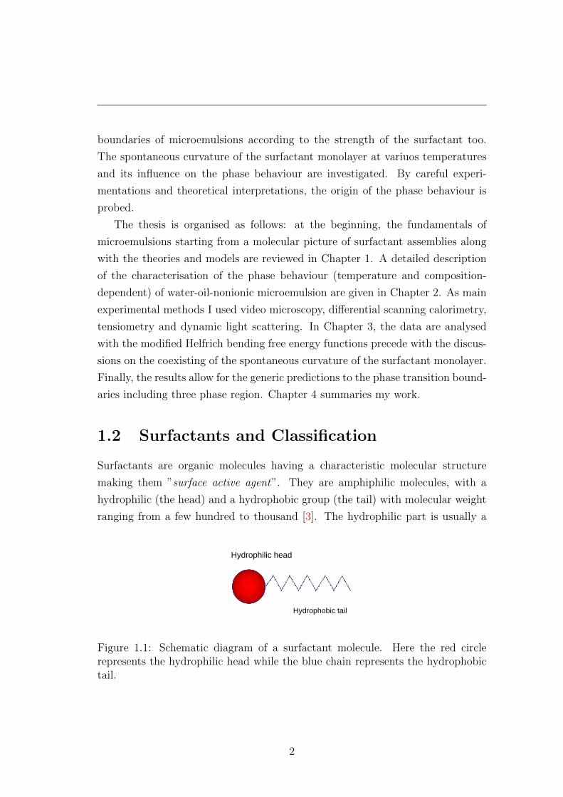
1.1 Schematic diagram of a surfactant molecule. Here the red circle

represents the hydrophilic head while the blue chain represents the

hydrophobic tail. . . . . . . . . . . . . . . . . . . . . . . . . . . . 2

1.2 Surfactant classification according to the nature of the hydrophilic

group and examples. The red colored part represents the hy-

drophilic head and the blue colored part represents the hydropho-

bic chains of the surfactant. . . . . . . . . . . . . . . . . . . . . . 4

1.3 Schematic diagram of surfactant molecules at the air-water inter-

face as well as inside water (blue color) (a) at concentration below

CMC : surfactant monolayer formation at air-water interface and

monomers in bulk water. The hydrophilic heads prefer water while

the hydrophobic tails try to avoid water and (b) at concentrations

above CMC: micelles (spherical aggregates) with hydrophilic heads

towards water and hydrophobic tails inside the micelle are formed. 5

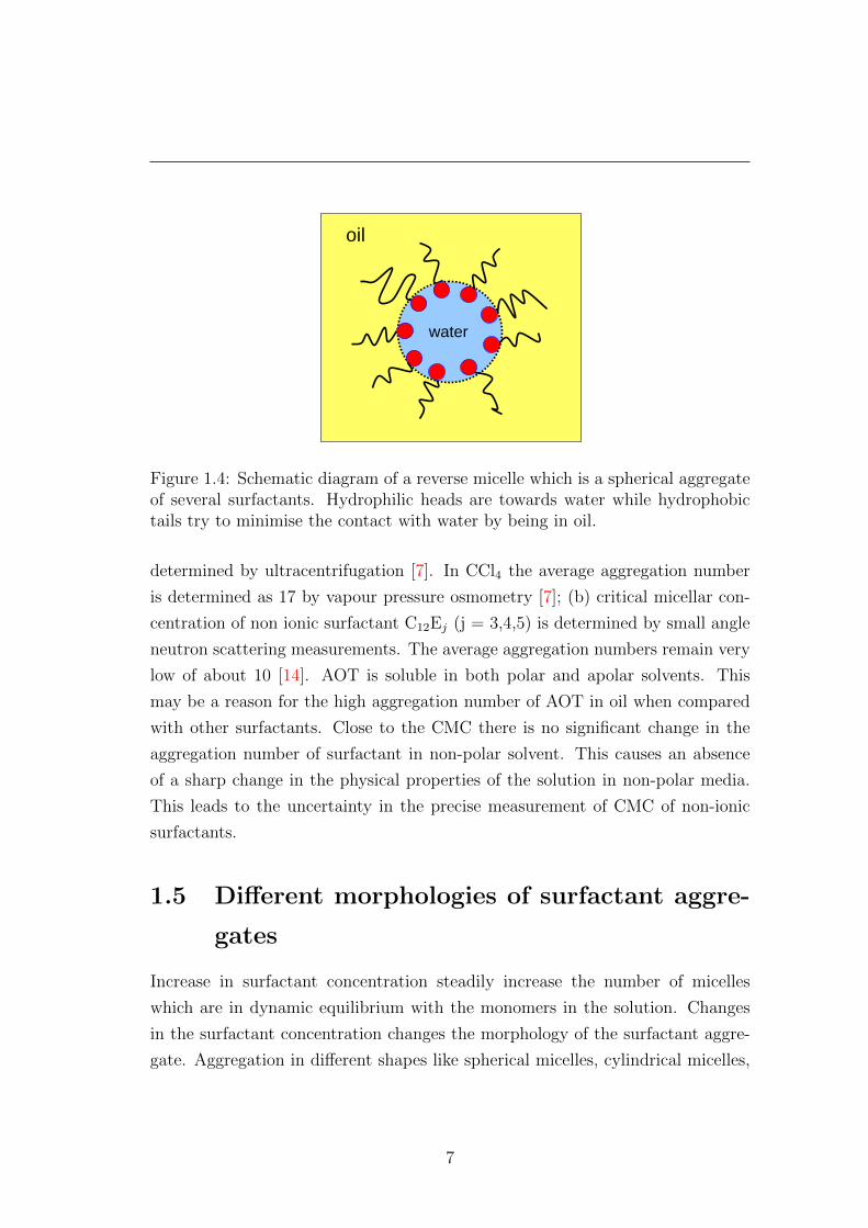
1.4 Schematic diagram of a reverse micelle which is a spherical aggre-

gate of several surfactants. Hydrophilic heads are towards water

while hydrophobic tails try to minimise the contact with water by

being in oil. . . . . . . . . . . . . . . . . . . . . . . . . . . . . . . 7

ix

LIST OF FIGURES

1.5 Sketches of different self-assembled structures of surfactant in wa-

ter. (a) Spherical micelle with hydrophobic core and hydrophilic

surface. The radius of the core is approximately equal to the length

of the hydrophobic chain (lmax). (b) In reverse/inverted micelles

the hydrocarbon tails are organised towards the oil medium, while

the head groups are inside the micelle. Inverted structures can

be cylinders or vesicles too. (c) Cylindrical micelles with a cross-

section similar to spherical micelles. They are usually polydisperse

due to the incorporation of more surfactants, causing the cylinder

grow. (d) Bicontinuous cubic structure with interconnected mono-

layer channels separating both oil and water continuous medium.

(e) In lamellar structure or planar bilayer, the bilayer thickness is

nearly 1.6 times lmax [1]. The plane layers separates the continu-

ous oil and water medium without any channels in the surfactant

monolayer and (f) Vesicles are formed by several closed bilayers,

without any connection between adjacent bilayers. The aqueous

compartment is isolated from the oil compartment. . . . . . . . . 9

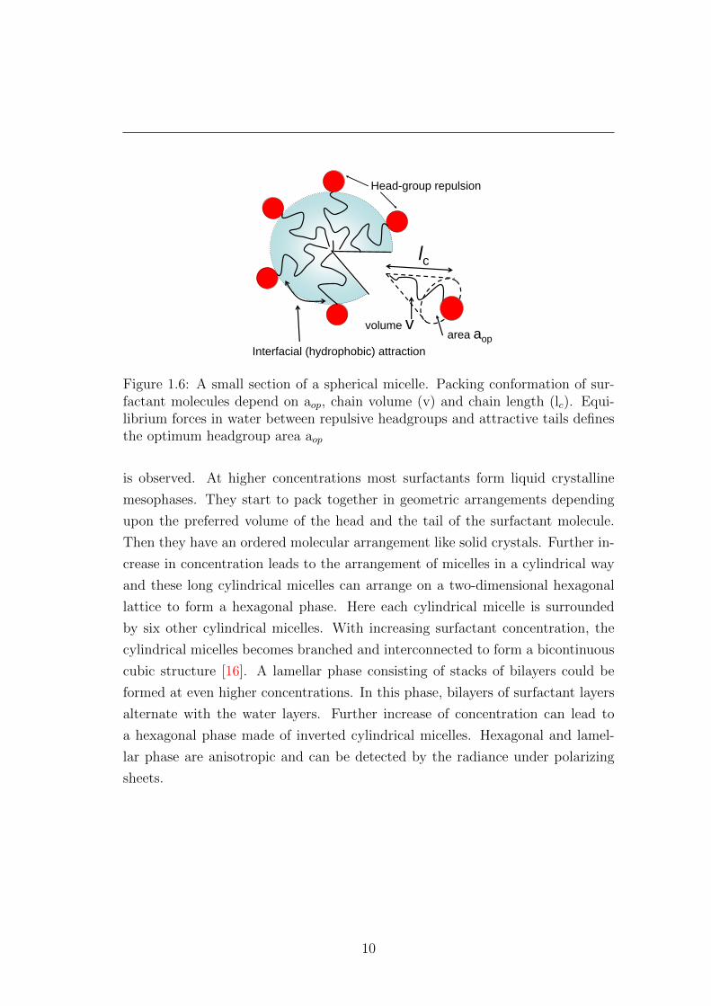
1.6 A small section of a spherical micelle. Packing conformation of

surfactant molecules depend on aop, chain volume (v) and chain

length (lc). Equilibrium forces in water between repulsive head-

groups and attractive tails defines the optimum headgroup area

aop . . . . . . . . . . . . . . . . . . . . . . . . . . . . . . . . . . . 10

1.7 Packing parameters, parameter shape and the various self assem-

bled structures formed by surfactant in water. Hydrophilic part is

exposed to water and the hydrophobic part is shielded away from

water. . . . . . . . . . . . . . . . . . . . . . . . . . . . . . . . . . 11

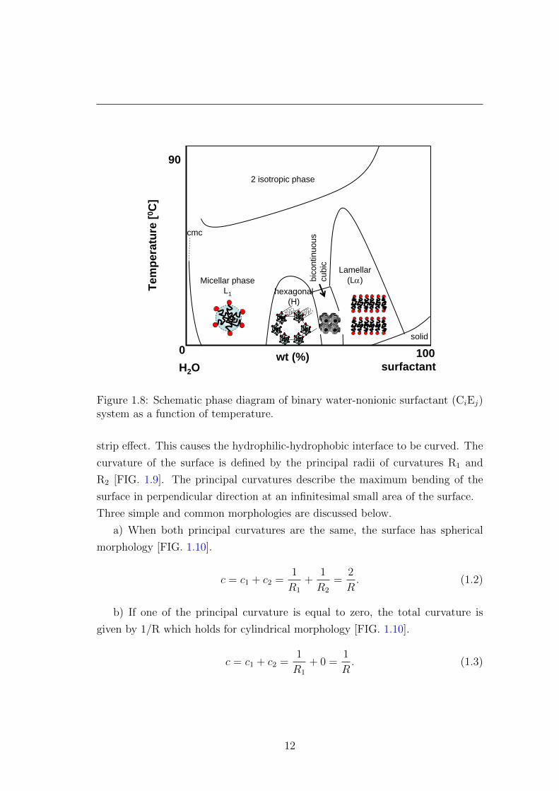
1.8 Schematic phase diagram of binary water-nonionic surfactant (CiEj)

system as a function of temperature. . . . . . . . . . . . . . . . . 12

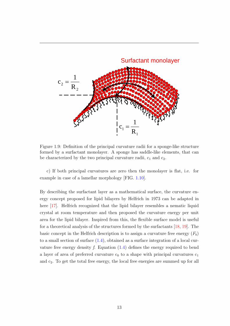
1.9 Definition of the principal curvature radii for a sponge-like struc-

ture formed by a surfactant monolayer. A sponge has saddle-like

elements, that can be characterized by the two principal curvature

radii, c1 and c2. . . . . . . . . . . . . . . . . . . . . . . . . . . . 13

x

LIST OF FIGURES

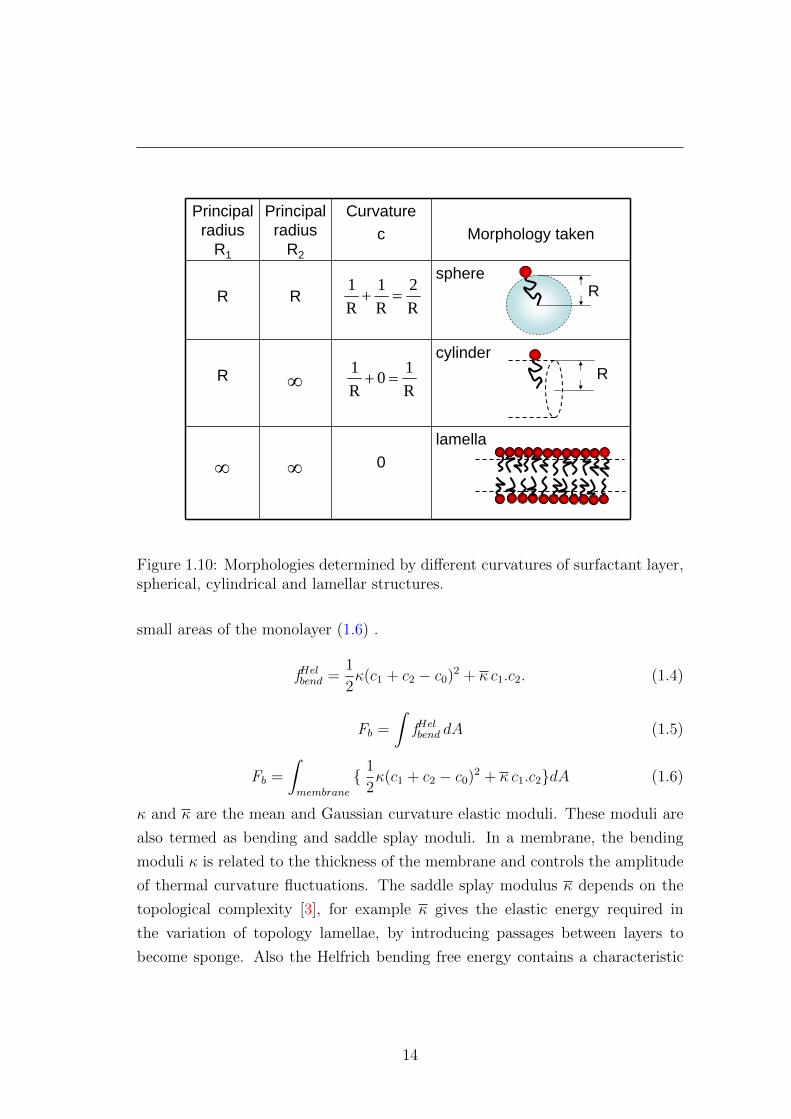
1.10 Morphologies determined by different curvatures of surfactant layer,

spherical, cylindrical and lamellar structures. . . . . . . . . . . . . 14

1.11 Curved interface formed by hydrophilic heads and hydrophobic

chains of surfactant molecules of a swollen inverted micelle with

oil (yellow) in water (blue). . . . . . . . . . . . . . . . . . . . . . 15

1.12 Schematic diagram of changing size of the polar region of a non-

ionic surfactant molecule with changing hydration. Blue color rep-

resents hydrated water molecules. . . . . . . . . . . . . . . . . . . 16

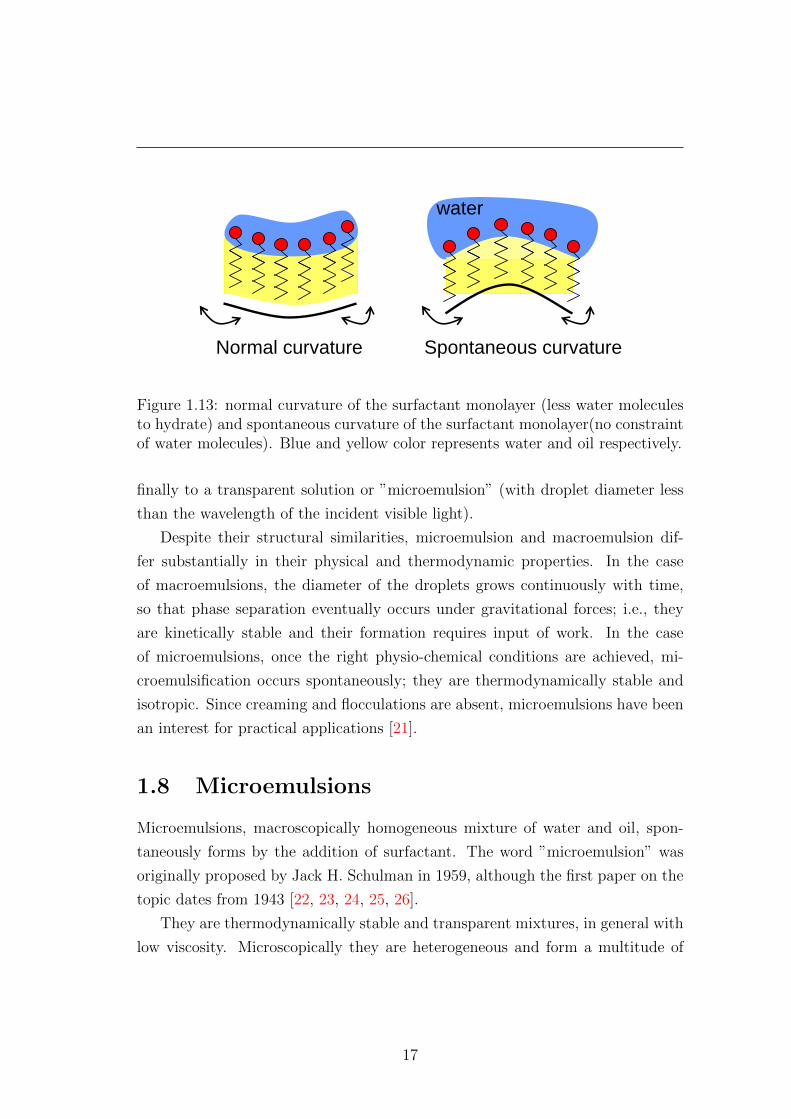
1.13 normal curvature of the surfactant monolayer (less water molecules

to hydrate) and spontaneous curvature of the surfactant mono-

layer(no constraint of water molecules). Blue and yellow color

represents water and oil respectively. . . . . . . . . . . . . . . . . 17

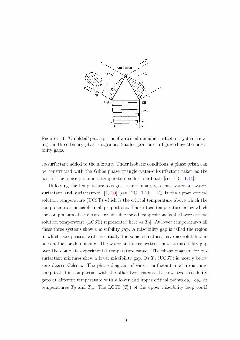
1.14 ’Unfolded’ phase prism of water-oil-nonionic surfactant system show-

ing the three binary phase diagrams. Shaded portions in figure

show the miscibility gaps. . . . . . . . . . . . . . . . . . . . . . . 19

1.15 Schematic phase prism for a water-oil-nonionic surfactant system

with broken critical lines. Macro-state of the microemulsion sam-

ple is sketched in the left side. For a description see the text.

Figure adapted from [2] . . . . . . . . . . . . . . . . . . . . . . . 20

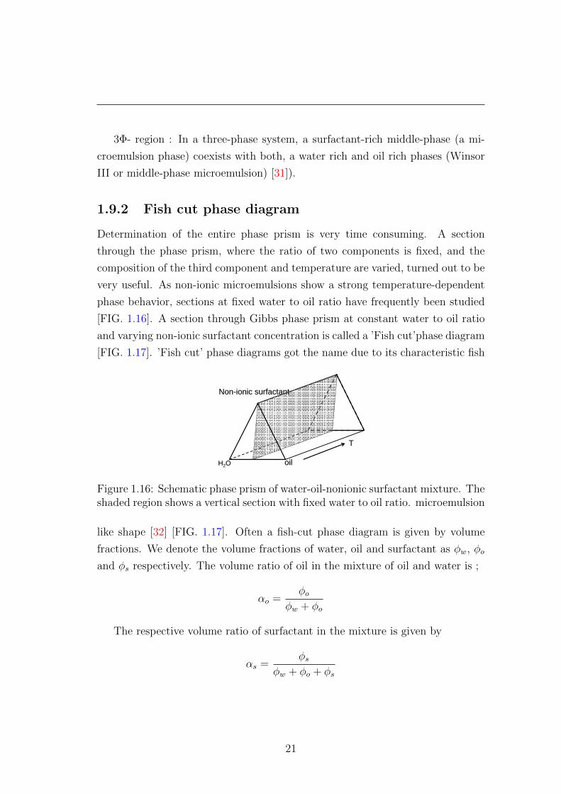
1.16 Schematic phase prism of water-oil-nonionic surfactant mixture.

The shaded region shows a vertical section with fixed water to oil

ratio. microemulsion . . . . . . . . . . . . . . . . . . . . . . . . . 21

1.17 Schematic ’fish cut’ phase diagram of a non-ionic microemulsion

with equal water to oil proportion as a function of surfactant con-

centration. The ’body’ of the fish has a surfactant-rich phase coex-

isting with a water and a oil-rich phase, from a temperature region

Tl to Tu (marked with dashed line). The ’tail’ of the fish has a

single phase region starting from φs towards higher φs. On the

either side of the body of the fish, a microemulsion phase coexist

with a water-rich or oil-rich phase. . . . . . . . . . . . . . . . . . 22

1.18 Comparison of the phase diagrams of microemulsions with a weak

(C4E1) and a strong (C12E5) surfactant. . . . . . . . . . . . . . . 24

xi

LIST OF FIGURES

1.19 Oil (shaded) and water (unshaded) domains generated by the Voronoi

process. Heavy lines denote the surfactant monolayer . . . . . . . 25

1.20 Array of cubical cells randomly filled with water (shaded) and oil

(white). Surfactants reside on the dark lines separating oil and

water domains. . . . . . . . . . . . . . . . . . . . . . . . . . . . . 26

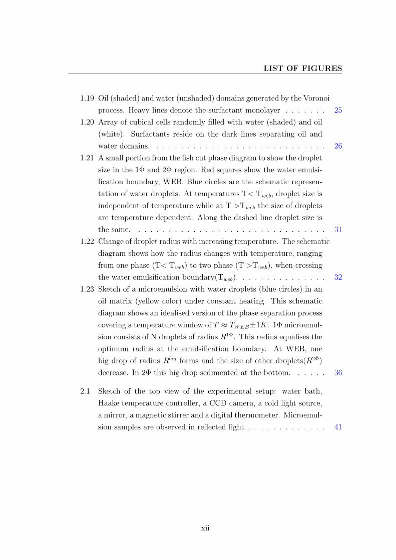
1.21 A small portion from the fish cut phase diagram to show the droplet

size in the 1Φ and 2Φ region. Red squares show the water emulsi-

fication boundary, WEB. Blue circles are the schematic represen-

tation of water droplets. At temperatures T< Tweb, droplet size is

independent of temperature while at T >Tweb the size of droplets

are temperature dependent. Along the dashed line droplet size is

the same. . . . . . . . . . . . . . . . . . . . . . . . . . . . . . . . 31

1.22 Change of droplet radius with increasing temperature. The schematic

diagram shows how the radius changes with temperature, ranging

from one phase (T< Tweb) to two phase (T >Tweb), when crossing

the water emulsification boundary(Tweb). . . . . . . . . . . . . . . 32

1.23 Sketch of a microemulsion with water droplets (blue circles) in an

oil matrix (yellow color) under constant heating. This schematic

diagram shows an idealised version of the phase separation process

covering a temperature window of T ≈ TWEB±1K. 1Φ microemul-

sion consists of N droplets of radius R1Φ. This radius equalises the

optimum radius at the emulsification boundary. At WEB, one

big drop of radius Rbig forms and the size of other droplets(R2Φ)

decrease. In 2Φ this big drop sedimented at the bottom. . . . . . 36

2.1 Sketch of the top view of the experimental setup: water bath,

Haake temperature controller, a CCD camera, a cold light source,

a mirror, a magnetic stirrer and a digital thermometer. Microemul-

sion samples are observed in reflected light. . . . . . . . . . . . . . 41

xii

LIST OF FIGURES

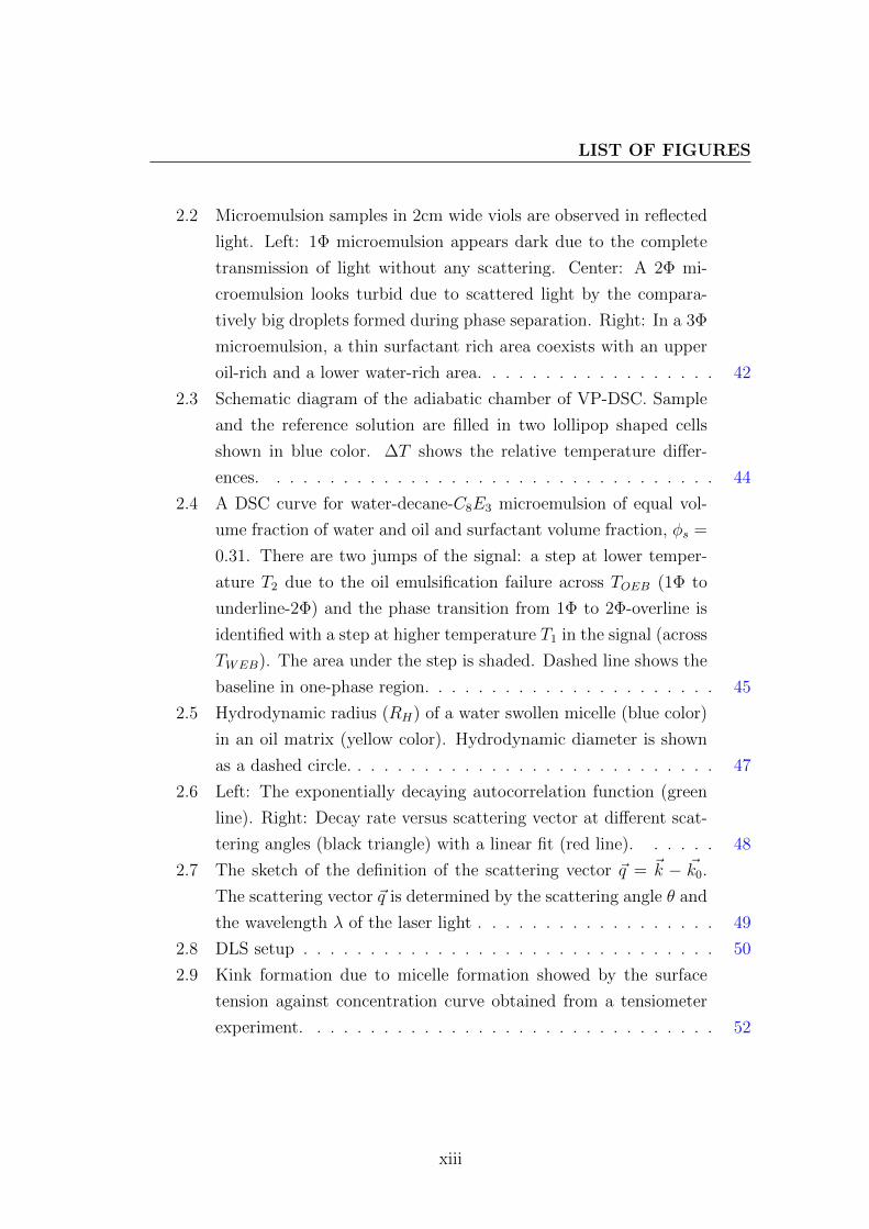
2.2 Microemulsion samples in 2cm wide viols are observed in reflected

light. Left: 1Φ microemulsion appears dark due to the complete

transmission of light without any scattering. Center: A 2Φ mi-

croemulsion looks turbid due to scattered light by the compara-

tively big droplets formed during phase separation. Right: In a 3Φ

microemulsion, a thin surfactant rich area coexists with an upper

oil-rich and a lower water-rich area. . . . . . . . . . . . . . . . . . 42

2.3 Schematic diagram of the adiabatic chamber of VP-DSC. Sample

and the reference solution are filled in two lollipop shaped cells

shown in blue color. ∆T shows the relative temperature differ-

ences. . . . . . . . . . . . . . . . . . . . . . . . . . . . . . . . . . 44

2.4 A DSC curve for water-decane-C8E3 microemulsion of equal vol-

ume fraction of water and oil and surfactant volume fraction, φs =

0.31. There are two jumps of the signal: a step at lower temper-

ature T2 due to the oil emulsification failure across TOEB (1Φ to

underline-2Φ) and the phase transition from 1Φ to 2Φ-overline is

identified with a step at higher temperature T1 in the signal (across

TWEB). The area under the step is shaded. Dashed line shows the

baseline in one-phase region. . . . . . . . . . . . . . . . . . . . . . 45

2.5 Hydrodynamic radius (RH) of a water swollen micelle (blue color)

in an oil matrix (yellow color). Hydrodynamic diameter is shown

as a dashed circle. . . . . . . . . . . . . . . . . . . . . . . . . . . . 47

2.6 Left: The exponentially decaying autocorrelation function (green

line). Right: Decay rate versus scattering vector at different scat-

tering angles (black triangle) with a linear fit (red line). . . . . . 48

2.7 The sketch of the definition of the scattering vector ~q = ~k − ~k0.

The scattering vector ~q is determined by the scattering angle θ and

the wavelength λ of the laser light . . . . . . . . . . . . . . . . . . 49

2.8 DLS setup . . . . . . . . . . . . . . . . . . . . . . . . . . . . . . . 50

2.9 Kink formation due to micelle formation showed by the surface

tension against concentration curve obtained from a tensiometer

experiment. . . . . . . . . . . . . . . . . . . . . . . . . . . . . . . 52

xiii

LIST OF FIGURES

2.10 (a) Schematic diagram of du Nouy ring. The ring registers the

contact with the liquid surface and is pushed through the liquid

surface to a few millimeters down. Then it is pulled up until the

maximum Force is reached. (b) Schematic diagram of a Wilhelmy

plate during surface tension measurement. The plate is wetted by

a length l and makes an angleθ with the liquid surface. A force F

acts due to the contact with liquid. . . . . . . . . . . . . . . . . . 53

3.1 Experimental value of the TWEB for 1:1 water: oil microemulsion,

under cooling and heating in a water bath. . . . . . . . . . . . . . 56

3.2 Microemulsion fish-cut phase diagram with 1:1 water-decane. Wa-

ter emulsification boundary, WEB [blue squares] and oil emulsifi-

cation boundary, OEB [green squares] are shown for samples with

varying surfactant concentration and with increasing temperature. 57

3.3 Microemulsion phase diagram with 3:7 (black squares) and 7:3

(green triangles) water-decane. TWEB [solid symbols] and TOEB

[open symbols] are shown for microemulsion samples with increas-

ing surfactant concentration. . . . . . . . . . . . . . . . . . . . . . 58

3.4 Temperature of the water emulsification (TWEB) (solid circles)

and oil emulsification (TOEB) (open circles) boundaries for water-

decane-C8E3 microemulsion with φs = 35% (green) and varying

oil to water + oil ratio; TWEB and TOEB for the same ingredient

sample with φs = 40% (blue) and varying αo; TWEB and TOEB at

varying αo for microemulsion samples with φs = 50% (orange). . . 59

xiv

LIST OF FIGURES

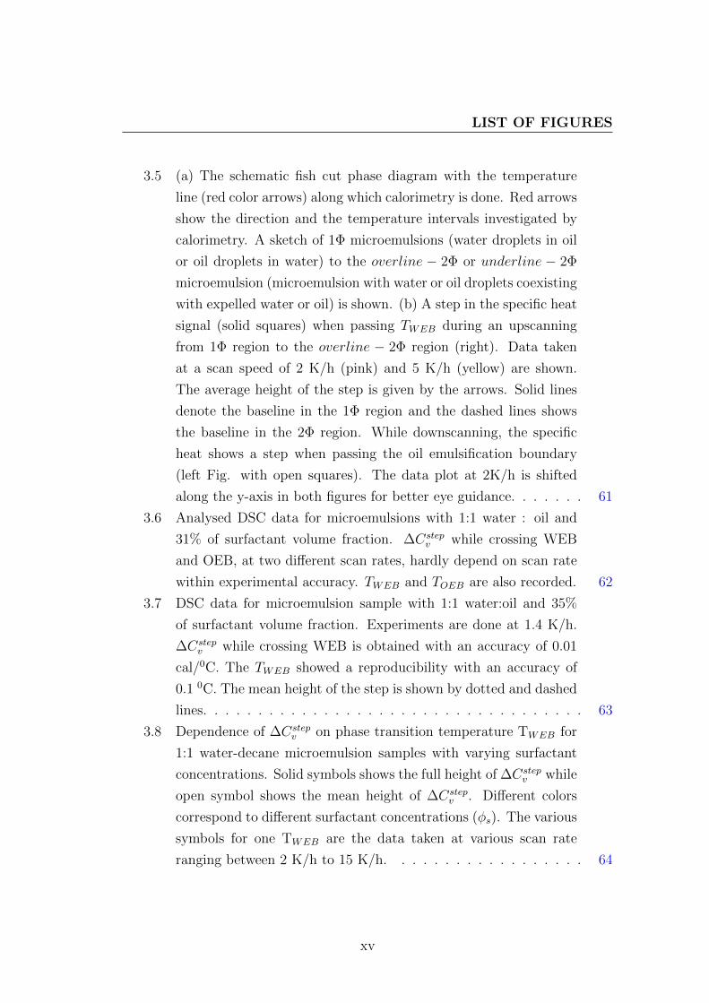
3.5 (a) The schematic fish cut phase diagram with the temperature

line (red color arrows) along which calorimetry is done. Red arrows

show the direction and the temperature intervals investigated by

calorimetry. A sketch of 1Φ microemulsions (water droplets in oil

or oil droplets in water) to the overline − 2Φ or underline − 2Φ

microemulsion (microemulsion with water or oil droplets coexisting

with expelled water or oil) is shown. (b) A step in the specific heat

signal (solid squares) when passing TWEB during an upscanning

from 1Φ region to the overline − 2Φ region (right). Data taken

at a scan speed of 2 K/h (pink) and 5 K/h (yellow) are shown.

The average height of the step is given by the arrows. Solid lines

denote the baseline in the 1Φ region and the dashed lines shows

the baseline in the 2Φ region. While downscanning, the specific

heat shows a step when passing the oil emulsification boundary

(left Fig. with open squares). The data plot at 2K/h is shifted

along the y-axis in both figures for better eye guidance. . . . . . . 61

3.6 Analysed DSC data for microemulsions with 1:1 water : oil and

31% of surfactant volume fraction. ∆Cstepv while crossing WEB

and OEB, at two different scan rates, hardly depend on scan rate

within experimental accuracy. TWEB and TOEB are also recorded. 62

3.7 DSC data for microemulsion sample with 1:1 water:oil and 35%

of surfactant volume fraction. Experiments are done at 1.4 K/h.

∆Cstepv while crossing WEB is obtained with an accuracy of 0.01

cal/0C. The TWEB showed a reproducibility with an accuracy of

0.1 0C. The mean height of the step is shown by dotted and dashed

lines. . . . . . . . . . . . . . . . . . . . . . . . . . . . . . . . . . . 63

3.8 Dependence of ∆Cstepv on phase transition temperature TWEB for

1:1 water-decane microemulsion samples with varying surfactant

concentrations. Solid symbols shows the full height of ∆Cstepv while

open symbol shows the mean height of ∆Cstepv . Different colors

correspond to different surfactant concentrations (φs). The various

symbols for one TWEB are the data taken at various scan rate

ranging between 2 K/h to 15 K/h. . . . . . . . . . . . . . . . . . 64

xv

LIST OF FIGURES

3.9 Dependence of ∆Cstepv on phase transition temperature TWEB for

sample with 3:7 water-to-oil ratio and varying surfactant concen-

tration. Different data points for the same TWEB denote the scat-

tering of the data at varying scan rates between 2K/h to 15 K/h.

Solid symbols show the full height of ∆Cstepv while open symbol

shows the mean height of ∆Cstepv . . . . . . . . . . . . . . . . . . . 64

3.10 Dependence of ∆Cstepv on phase transition temperature TWEB for

sample with 7:3 water-decane ratio and varying surfactant con-

centration ranging between 35% and 55% (different colored dia-

monds). Solid symbols show the full height of the step in the

specific heat ∆Cstepv , while open symbols show the mean height of

the step. The data at different scan rates on the same sample are

shown by the same colored symbols. . . . . . . . . . . . . . . . . 65

3.11 Mean height of the specific heat-step with increasing temperature

for water emulsification boundaries. The data correspond to three

different compositions : 7:3 water-decane (purple diamond), 1:1

water-decane (wine pentagons) and 3:7 water-decane microemul-

sion (orange circles). A third order polynomial fit is given for a

better eye guidance. . . . . . . . . . . . . . . . . . . . . . . . . . 65

3.12 Difference in the phase transition temperature obtained from visual

inspection (scattering) in water bath and microcalorimetry (DSC)

for microemulsion sample with equal water to oil ratio. The scan

rate is added in brackets. . . . . . . . . . . . . . . . . . . . . . . 66

3.13 Refractive index of the microemulsion samples with different sur-

factant concentrations at different temperatures. . . . . . . . . . . 67

3.14 Fish cut phase diagram of a 1:1 water-decane microemulsion as

a function of φs. TWEB and TOEB are shown by the blue and

black circles respectively. The temperatures at which samples are

investigated by DLS are marked by pink crosses. The macroscopic

appearence of the microemulsion is sketched too. . . . . . . . . . . 68

3.15 Hydrodynamic radius of oil/water domains obtained from DLS.

Microemulsion samples with 1:1 water-decane and three different

surfactant concentrations are used. . . . . . . . . . . . . . . . . . 69

xvi

LIST OF FIGURES

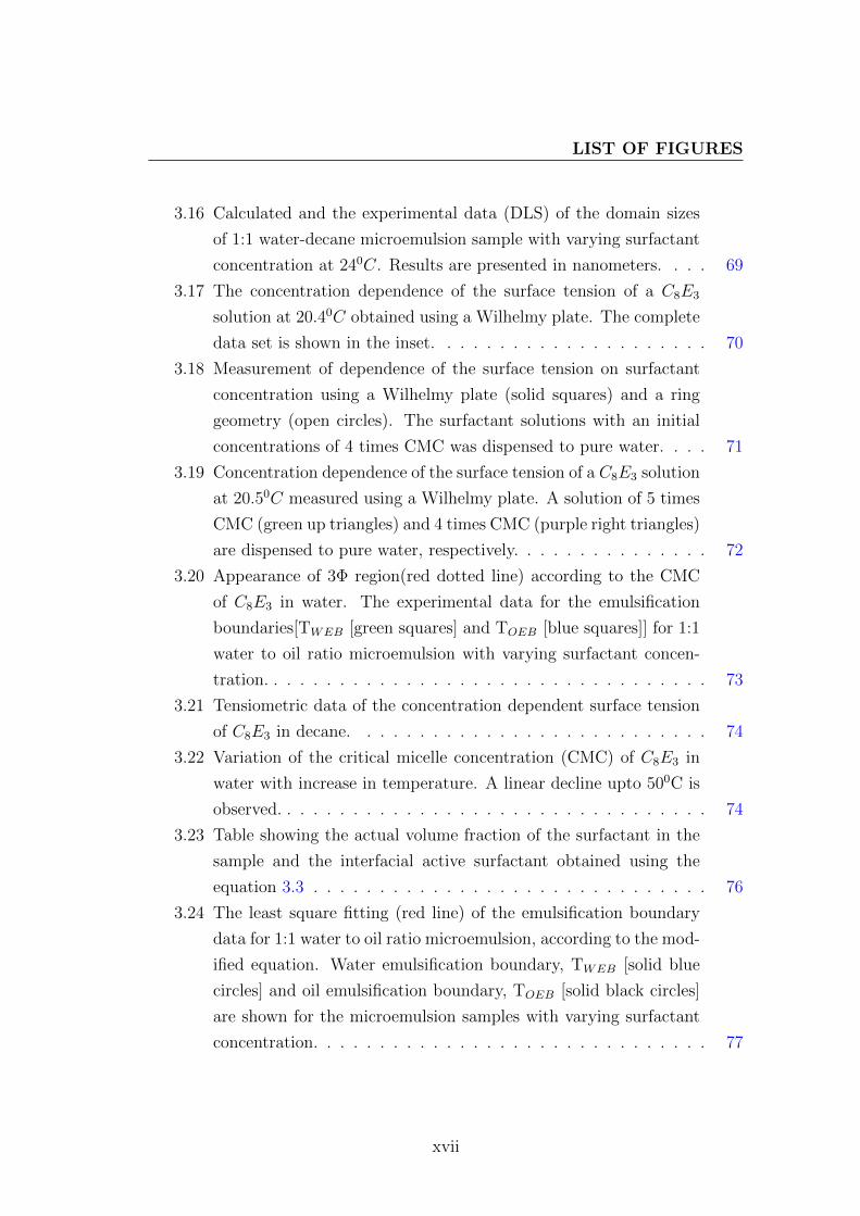
3.16 Calculated and the experimental data (DLS) of the domain sizes

of 1:1 water-decane microemulsion sample with varying surfactant

concentration at 240C. Results are presented in nanometers. . . . 69

3.17 The concentration dependence of the surface tension of a C8E3

solution at 20.40C obtained using a Wilhelmy plate. The complete

data set is shown in the inset. . . . . . . . . . . . . . . . . . . . . 70

3.18 Measurement of dependence of the surface tension on surfactant

concentration using a Wilhelmy plate (solid squares) and a ring

geometry (open circles). The surfactant solutions with an initial

concentrations of 4 times CMC was dispensed to pure water. . . . 71

3.19 Concentration dependence of the surface tension of a C8E3 solution

at 20.50C measured using a Wilhelmy plate. A solution of 5 times

CMC (green up triangles) and 4 times CMC (purple right triangles)

are dispensed to pure water, respectively. . . . . . . . . . . . . . . 72

3.20 Appearance of 3Φ region(red dotted line) according to the CMC

of C8E3 in water. The experimental data for the emulsification

boundaries[TWEB [green squares] and TOEB [blue squares]] for 1:1

water to oil ratio microemulsion with varying surfactant concen-

tration. . . . . . . . . . . . . . . . . . . . . . . . . . . . . . . . . . 73

3.21 Tensiometric data of the concentration dependent surface tension

of C8E3 in decane. . . . . . . . . . . . . . . . . . . . . . . . . . . 74

3.22 Variation of the critical micelle concentration (CMC) of C8E3 in

water with increase in temperature. A linear decline upto 500C is

observed. . . . . . . . . . . . . . . . . . . . . . . . . . . . . . . . . 74

3.23 Table showing the actual volume fraction of the surfactant in the

sample and the interfacial active surfactant obtained using the

equation 3.3 . . . . . . . . . . . . . . . . . . . . . . . . . . . . . . 76

3.24 The least square fitting (red line) of the emulsification boundary

data for 1:1 water to oil ratio microemulsion, according to the mod-

ified equation. Water emulsification boundary, TWEB [solid blue

circles] and oil emulsification boundary, TOEB [solid black circles]

are shown for the microemulsion samples with varying surfactant

concentration. . . . . . . . . . . . . . . . . . . . . . . . . . . . . . 77

xvii

LIST OF FIGURES

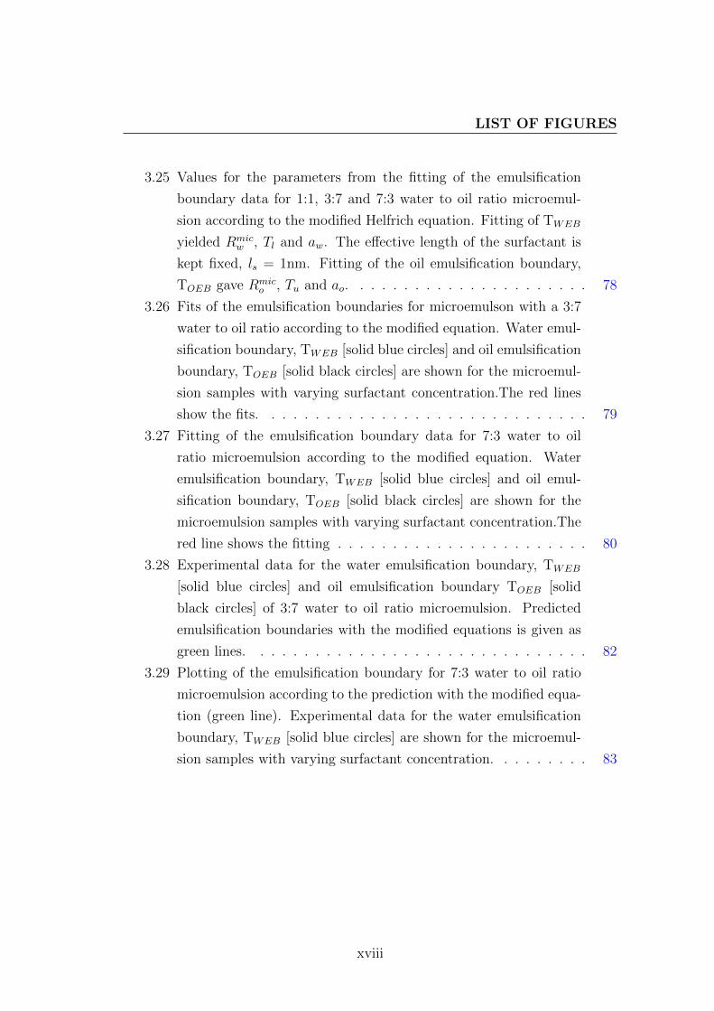
3.25 Values for the parameters from the fitting of the emulsification

boundary data for 1:1, 3:7 and 7:3 water to oil ratio microemul-

sion according to the modified Helfrich equation. Fitting of TWEB

yielded Rmicw , Tl and aw. The effective length of the surfactant is

kept fixed, ls = 1nm. Fitting of the oil emulsification boundary,

TOEB gave Rmico , Tu and ao. . . . . . . . . . . . . . . . . . . . . . 78

3.26 Fits of the emulsification boundaries for microemulson with a 3:7

water to oil ratio according to the modified equation. Water emul-

sification boundary, TWEB [solid blue circles] and oil emulsification

boundary, TOEB [solid black circles] are shown for the microemul-

sion samples with varying surfactant concentration.The red lines

show the fits. . . . . . . . . . . . . . . . . . . . . . . . . . . . . . 79

3.27 Fitting of the emulsification boundary data for 7:3 water to oil

ratio microemulsion according to the modified equation. Water

emulsification boundary, TWEB [solid blue circles] and oil emul-

sification boundary, TOEB [solid black circles] are shown for the

microemulsion samples with varying surfactant concentration.The

red line shows the fitting . . . . . . . . . . . . . . . . . . . . . . . 80

3.28 Experimental data for the water emulsification boundary, TWEB

[solid blue circles] and oil emulsification boundary TOEB [solid

black circles] of 3:7 water to oil ratio microemulsion. Predicted

emulsification boundaries with the modified equations is given as

green lines. . . . . . . . . . . . . . . . . . . . . . . . . . . . . . . 82

3.29 Plotting of the emulsification boundary for 7:3 water to oil ratio

microemulsion according to the prediction with the modified equa-

tion (green line). Experimental data for the water emulsification

boundary, TWEB [solid blue circles] are shown for the microemul-

sion samples with varying surfactant concentration. . . . . . . . . 83

xviii

LIST OF FIGURES

3.30 Experimental data for the evolution of water and oil emulsification

boundaries with temperature and varying αo are given by solid

and open circles respectively. Surfactant concentration is fixed

at 35% (green), 40% (blue) and 50% (orange). The predictions

(lines) for the water emulsification boundaries (solid lines) and

the oil emulsification boundaries (dotted lines) according to the

modified equation for the three different surfactant concentrations

are shown. The dashed line shows the temperature Tl and Tu.

Microstructure of the sample at various temperatures are sketched. 84

3.31 Spontaneous curvature as a function of temperature for a mi-

croemulsion with equal proportion of water to oil. At higher and

lower temperatures the water and oil droplet reaches inverse micel-

lar radii Rwmic and micellar radii Ro

mic respectively. ′a′w and ′a′o gives

the scaling of the surfactant morphology from a droplet structure

to inverse micelle and micelle. . . . . . . . . . . . . . . . . . . . . 86

3.32 Sketch of the coexisting spontaneous curvature as a function of

temperature for a microemulsion with equal proportion of water

and oil. At higher and lower temperatures the water and oil droplet

reaches inverse micellar radii Rwmic and micellar radii Ro

mic respec-

tively. ′a′w and ′a′o gives the scaling of the surfactant morphology

from a droplet structure to inverse micelle/micelle. . . . . . . . . 87

3.33 Temperature dependent variation of the specific heat for equal wa-

ter to oil ratio and surfactant concentration φs = 0.31 (orange dia-

monds), φs = 0.45 (purple diamonds) and φs = 0.55 (dark cyan di-

amonds). Data has been subtracted with a baseline. Mean height

of the specific heat and the prediction (with the pre-factor) are

shown. The thermograms are taken at 5 K/h across water emulsi-

fication boundary. . . . . . . . . . . . . . . . . . . . . . . . . . . . 90

xix

LIST OF FIGURES

3.34 Experimental data from DSC (open circles) and the prediction to

the height of the specific heat-step according to Eq.3.12 (dashed

line) and Eq.3.13 with prefactor (solid line) with increasing phase

transition temperature for (a) 1:1 water to oil ratio microemulsion;

(b) 3:7 water to oil ratio microemulsion and (c) 7:3 water to oil

ratio microemulsion. . . . . . . . . . . . . . . . . . . . . . . . . . 92

3.35 Experimental data (open circles) for the the mean height of the

specific heat-step for with increasing TWEB for (a) 1:1 water to oil

ratio microemulsion (purple) ; (b)3:7 water to oil ratio microemul-

sion (black) and (c) 7:3 water to oil ratio microemulsion (blue).

Theoretical prediction of the height of the specific heat-step with

prefactor are shown by solid lines (magenta) for the three different

data. . . . . . . . . . . . . . . . . . . . . . . . . . . . . . . . . . . 94

3.36 The mean height of the specific heat-step of microemulsion sam-

ples with three different αo = αo/(αo + αw) and fixed surfactant

volume fraction 0.35: from the differential scanning calorimetry

(open circles) and according to the prediction Eq.3.13(cross). . . 95

3.37 Experimental data for the TWEB (blue circles) and TOEB (black

circles) for the C4E1 - octane - water microemulsion. A 10%

surfactant-volume fraction the sample is in 2Φ. Dotted line sepa-

rates 2Φ and 3Φ. Green line shows the prediction. . . . . . . . . 96

xx

Chapter 1

Introduction

Phase studies are inevitable for the basic understanding of general phase be-

haviour and kinetics of the structural changes of a system. This is not only of

fundamental interest but also is very important for any industrial and techno-

logical processes. Phase diagrams for microemulsions are quite complex since

there are at least three components- water, oil and surfactant. These structured

fluids have a readily deformable surfactant interface, which bend either towards

water or oil or both. A wide range surfactants can produce microemulsion. I

will introduce non-ionic microemulsion that has served as model system for this

work. Properties of non-ionic surfactants are sensitive to the changes in the tem-

perature. Non-ionic microemulsion goes through a multitude of micro and macro

structures in less than 200C. The generic phase behaviours, dominated by the

surfactant properties, for microemulsion are evaluated.

1.1 Motivation and Objectives

It was the goal of this work to investigate the phase behaviour of non-ionic mi-

croemulsions and predict the phase transition boundaries including the three-

phase region using a modified Helfrich free energy. The phase behaviour is ap-

proached in two ways : (a) composition dependent and (b) through the bending

free energy. The consistency of the phase transition boundaries in these two differ-

ent approaches are checked. Experiments and predictions are examined for phase

1

boundaries of microemulsions according to the strength of the surfactant too.

The spontaneous curvature of the surfactant monolayer at variuos temperatures

and its influence on the phase behaviour are investigated. By careful experi-

mentations and theoretical interpretations, the origin of the phase behaviour is

probed.

The thesis is organised as follows: at the beginning, the fundamentals of

microemulsions starting from a molecular picture of surfactant assemblies along

with the theories and models are reviewed in Chapter 1. A detailed description

of the characterisation of the phase behaviour (temperature and composition-

dependent) of water-oil-nonionic microemulsion are given in Chapter 2. As main

experimental methods I used video microscopy, differential scanning calorimetry,

tensiometry and dynamic light scattering. In Chapter 3, the data are analysed

with the modified Helfrich bending free energy functions precede with the discus-

sions on the coexisting of the spontaneous curvature of the surfactant monolayer.

Finally, the results allow for the generic predictions to the phase transition bound-

aries including three phase region. Chapter 4 summaries my work.

1.2 Surfactants and Classification

Surfactants are organic molecules having a characteristic molecular structure

making them ”surface active agent”. They are amphiphilic molecules, with a

hydrophilic (the head) and a hydrophobic group (the tail) with molecular weight

ranging from a few hundred to thousand [3]. The hydrophilic part is usually a

Hydrophilic head

Hydrophobic tail

Figure 1.1: Schematic diagram of a surfactant molecule. Here the red circlerepresents the hydrophilic head while the blue chain represents the hydrophobictail.

2

non-ionic (polar) or an ionic group attached covalently to the hydrophobic part

which is usually a long hydrocarbon chain. The hydrophilic region associates

with the hydrogen bond network of water [4], whereas the hydrophobic region

in general includes hydrocarbon chain which do not favors contact with water.

Water molecules are more ordered around a hydrophobic group than in bulk wa-

ter. Therefore it is entropically unfavorable to restructure or reorient the water

molecules near to a nonpolar molecule, giving it a hydrophobic nature. Briefly,

a single surfactant molecule has both a water soluble and a water insoluble part.

A surfactant molecule, in general is picturised with a head and tail as shown in

FIG 1.

Depending on the nature of the hydrophilic group, surfactants are further classi-

fied [3, 5, 6] as

1. Anionic: The surface active part bears negative charge. The relatively low

cost in manufacture makes them the most sort after surfactant in the industry.

Sodium dodecylsulfate (SDS) is a well known example with the molecular formula

CH3(CH2)11SO4− Na+. In here the dodecane is insoluble in water (hydrophobic

tail), whereas the ionisable property makes the sulphate portion strongly hy-

drophilic [see FIG. 1.2]. Other examples are RCOO−Na+ (soap) and RSO3−Na+

(sulfonates).

2. Cationic: The surface active part bears positive charge. They are non-

biodegradable and are used as bactericides. Due to the tendency to be adsorbed

at negatively charged surfaces, they are anticorrosive and antistatic agents [see

FIG. 1.2]. Examples: RNH3+Cl− (salt of long-chain amine), RN(CH3)3

+Cl−

(quaternary ammonium chloride), CTAB.

3. Zwitterionic: These surfactants contain both cationic and anionic groups.

In general their properties highly depend on the pH of the solution [see FIG. 1.2].

Example: RH+H2CH2COO− (long-chain amino acid), RN+(CH3)2CH2CH2SO3−

(sulfobetaine).

4. Non-ionic: Apparently bears no ionic charge but are polar. Two important

classes of non-ionic surfactants are the ones based on ethylene oxide, referred to

3

as ethoxylated surfactants and the multihydroxy products such as glycerols and

sucrose esters. The former category has a general form H(CH2)i(OCH2CH2)jOH

(abbreviated as CiEj). Octyl triethylene glycol ether (C8E3) is an example of

an ethoxylated surfactant [see FIG. 1.2]. The carbon chains form the hydropho-

bic tail while the ethylene oxide (EO) chains form the hydrophilic head. The

solubility of ethylene oxide chains highly depend on temperature. At a low tem-

perature, water is a good solvent for ethylene oxide chains due to hydrogen bond

formation. Increasing temperature causes high entropy leading to the breakage of

these hydrogen bonds. This makes water a poor solvent for the same surfactant

at higher temperatures.

Anionic

Cationic

Zwitterionic

Nonionic

Sodium dodecylsulfate (SDS)

OO

P

O

OO

OCH2CH2N(CH3)3+

O-

Dipalmitoylphosphatidylcholine (lecithin)

Octyl triethylene glycol ether ( C8E3)

N+ Br

-

cetyltrimethylammonium bromide (CTAB)

S O- Na+O

O

O O O OH

Figure 1.2: Surfactant classification according to the nature of the hydrophilicgroup and examples. The red colored part represents the hydrophilic head andthe blue colored part represents the hydrophobic chains of the surfactant.

4

1.3 Surfactants in water

(a) C < CMC(a) C < CMC (b) C > CMC(b) C > CMC

Figure 1.3: Schematic diagram of surfactant molecules at the air-water interfaceas well as inside water (blue color) (a) at concentration below CMC : surfactantmonolayer formation at air-water interface and monomers in bulk water. Thehydrophilic heads prefer water while the hydrophobic tails try to avoid water and(b) at concentrations above CMC: micelles (spherical aggregates) with hydrophilicheads towards water and hydrophobic tails inside the micelle are formed.

Surfactants show distinct behavior while interacting with different solvents

due to the quite different solubility criterion within a molecule. To-date most in-

vestigations are focused on aqueous surfactant solutions [7], while a few research

are done on surfactants in non-aqueous media [8, 9]. At low concentration sur-

factant molecules exist as monomers in water. The hydrophilic groups strongly

interact with water while the hydrophobic alkyl chains try to avoid contact with

water. As the hydrophobic groups distort the arrangement of water molecules,

they increase the free energy of the system. Hydrophobic groups have to be

avoided to reduce this free energy. Surfactants achieve this state by self assem-

bling in different ways [FIG. 1.3, FIG. 1.5]. Along the water surface they spon-

taneously form a monolayer with hydrophilic part inside water and hydrophobic

part towards air [FIG. 1.3]. This could significantly alter the surface properties

of water and thereby cause a reduction in surface tension and thus decreasing the

free energy. Increasing the surfactant concentration saturates the water surface.

And any further increase in the concentration causes the molecules to dissolve in

water and thereby changes the way of arrangement of surfactant molecules. To

5

reduce water-tail contact, the system starts self-assembling. Surfactant molecules

aggregate in spherical forms with hydrophobic tails within the spheres and hy-

drophilic part towards water. These aggregates are called micelles [FIG. 1.3 (b)].

Typical micelle contains 50 to 100 monomers depending on the type of surfac-

tant. The critical concentration above which spontaneous formation of micelles

occurs is called critical micelle concentration (CMC). Further increase in sur-

factant concentration above CMC increases the number of micelles which are in

dynamic equilibrium with the monomers in the solution and the saturated water-

air interface. FIG. 1.3 shows the state of surfactant in water below and above

the critical micelle concentration. CMC is an important measure for surfactant

characterization.

1.4 Surfactants in non-polar solvent (oil)

The behavior of surfactants in nonpolar media is equally relevant in understand-

ing the characteristics of ternary mixtures, as well as for the applications in oil

recovery and the synthesis of colloidal particles [10, 11]. However, the information

of the physical properties of non-ionic surfactants in non-polar media is scarce.

The obvious difference between micelles in polar and non-polar media is the struc-

tural reversion, with polar core covered by hydrophobic tails known as reverse or

inverted micelle [see FIG. 1.4]. As mentioned before, the CMC in aqueous media

can be explained by the additional ordering of the water molecules upon addition

of surfactant. In contrast to this, in non-polar media the presence of surfactants

hardly induces structural changes to the solvent molecules [12]. The interaction of

the hydrophobic tails with solvent is also favourable with the other hydrophobic

tails. Hence surfactants do not migrate to the solvent-air interface. Furthermore,

air is highly hydrophobic. Therefore the head groups try to avoid air as well as the

solvent. The dipole-dipole interactions between the polar head groups lead to the

formation of small aggregates. Unlike the large micellar aggregate in water, ag-

gregation number in non-polar solvents is moderate, ranging from 7 to 30 [7, 13].

Moreover, the average life time of a molecule at the interface is lower due to a

high exchange rate between molecules molecularly dissolved and in aggregates.

The average aggregation number at 250C for (a)AOT in dodecane is around 28,

6

water

oil

Figure 1.4: Schematic diagram of a reverse micelle which is a spherical aggregateof several surfactants. Hydrophilic heads are towards water while hydrophobictails try to minimise the contact with water by being in oil.

determined by ultracentrifugation [7]. In CCl4 the average aggregation number

is determined as 17 by vapour pressure osmometry [7]; (b) critical micellar con-

centration of non ionic surfactant C12Ej (j = 3,4,5) is determined by small angle

neutron scattering measurements. The average aggregation numbers remain very

low of about 10 [14]. AOT is soluble in both polar and apolar solvents. This

may be a reason for the high aggregation number of AOT in oil when compared

with other surfactants. Close to the CMC there is no significant change in the

aggregation number of surfactant in non-polar solvent. This causes an absence

of a sharp change in the physical properties of the solution in non-polar media.

This leads to the uncertainty in the precise measurement of CMC of non-ionic

surfactants.

1.5 Different morphologies of surfactant aggre-

gates

Increase in surfactant concentration steadily increase the number of micelles

which are in dynamic equilibrium with the monomers in the solution. Changes

in the surfactant concentration changes the morphology of the surfactant aggre-

gate. Aggregation in different shapes like spherical micelles, cylindrical micelles,

7

lamellar structure, hexagonal, bicontinuous structure etc. have been observed. A

few morphologies are sketched in FIG. 1.5 [1].

Israelachvili et al. tried to predict these shapes in terms of geometrical shape

of the individual surfactant molecules. Therefore, Israelachvili introduced a di-

mensionless parameter called ’packing parameter ’, P. It can be defined as

P =v

aoplc(1.1)

where aop is the optimal head group area of the surfactant, v the hydrocarbon

chain volume and lc the chain length [FIG. 1.6].

In water, the surfactant layer experience opposing forces at the water-hydrocarbon

tail interface [FIG. 1.6]. Hydrophobic attractive force try to decrease the inter-

facial area whereas repulsive force try to increase the area ′a′ per molecule. This

result in an optimal interfacial area ’aop’ [3, 4]. Though often hard to quantify,

the ’packing parameter ’ P is useful to estimate the shape of surfactant aggregates.

Structures taken by surfactant molecules with different packing parameters are

shown in FIG. 1.7 and FIG. 1.5. Surfactants with charged headgroups get a large

head group area aop and thus P < 1/3 and they tend to form spherical micelles.

Those surfactants with smaller headgroup area such that 1/3 < v/aop lc < 1/2

cannot pack into spherical micelle but forms cylindrical (rod-like) micelles. An-

other category of surfactants possess bulky hydrocarbon chains and small head

groups but maintain the surface area at its optimal value. Their v/aop lc value

lie close to 1 and they form bilayers. Finally for surfactants with very small head

group areas and bulky hydrocarbon chains, the packing parameter value exceeds

unity and they form inverted micelles.

There are various factors affecting the geometric packing parameter, P. Since

we are focusing on non-ionic surfactants, the effect of temperature is the relevant

factor here. Changing the temperature can alter both aop and lc. Also in non-ionic

surfactant by changing the length of the polyethyleneoxide chains, aop is changed.

Then the monolayer structure and thereby the phase behavior varies too. FIG. 1.8

[15] shows a general phase diagram for non-ionic surfactant in water as a func-

tion of temperature. The surfactant molecules are dissolved in water until the

surfactant concentration reaches its CMC. Just above CMC, a micellar solution

8

a) Spherical micelle b) Reverse micelle

c) Cylindrical micelle

d) Bicontinuous cubic

e) Lamellar structure f) Vesicle

Figure 1.5: Sketches of different self-assembled structures of surfactant in water.(a) Spherical micelle with hydrophobic core and hydrophilic surface. The radiusof the core is approximately equal to the length of the hydrophobic chain (lmax).(b) In reverse/inverted micelles the hydrocarbon tails are organised towards theoil medium, while the head groups are inside the micelle. Inverted structures canbe cylinders or vesicles too. (c) Cylindrical micelles with a cross-section similarto spherical micelles. They are usually polydisperse due to the incorporationof more surfactants, causing the cylinder grow. (d) Bicontinuous cubic structurewith interconnected monolayer channels separating both oil and water continuousmedium. (e) In lamellar structure or planar bilayer, the bilayer thickness is nearly1.6 times lmax [1]. The plane layers separates the continuous oil and water mediumwithout any channels in the surfactant monolayer and (f) Vesicles are formed byseveral closed bilayers, without any connection between adjacent bilayers. Theaqueous compartment is isolated from the oil compartment.

9

lc

area aop

Head-group repulsion

Interfacial (hydrophobic) attraction

volume v

Figure 1.6: A small section of a spherical micelle. Packing conformation of sur-factant molecules depend on aop, chain volume (v) and chain length (lc). Equi-librium forces in water between repulsive headgroups and attractive tails definesthe optimum headgroup area aop

is observed. At higher concentrations most surfactants form liquid crystalline

mesophases. They start to pack together in geometric arrangements depending

upon the preferred volume of the head and the tail of the surfactant molecule.

Then they have an ordered molecular arrangement like solid crystals. Further in-

crease in concentration leads to the arrangement of micelles in a cylindrical way

and these long cylindrical micelles can arrange on a two-dimensional hexagonal

lattice to form a hexagonal phase. Here each cylindrical micelle is surrounded

by six other cylindrical micelles. With increasing surfactant concentration, the

cylindrical micelles becomes branched and interconnected to form a bicontinuous

cubic structure [16]. A lamellar phase consisting of stacks of bilayers could be

formed at even higher concentrations. In this phase, bilayers of surfactant layers

alternate with the water layers. Further increase of concentration can lead to

a hexagonal phase made of inverted cylindrical micelles. Hexagonal and lamel-

lar phase are anisotropic and can be detected by the radiance under polarizing

sheets.

10

Inverted micelleInverted truncated cone

> 1

Double-chain surfactants with very small head

group area or with long HC chain

bilayersCylinder

~ 1

Double chain surfactants with

small head group area

Cylindrical micelleTruncated cone

1/3 – 1/2

Small head group area

Spherical micellecone

< 1/3

Large head group area

Aggregate formedShapeP = v / (a0lc)Surfactant

Figure 1.7: Packing parameters, parameter shape and the various self assembledstructures formed by surfactant in water. Hydrophilic part is exposed to waterand the hydrophobic part is shielded away from water.

1.6 Helfrich free energy

Surfactants monolayers or bilayers are a physical realization of fluctuating sur-

faces. These monolayers are soft, flexible and incompressible. This is due to the

van der Waals forces, hydrophobic, hydrogen-bonding and screened electrostatic

interactions. These monolayers are very thin sheets with a height of 3-10 nm

depending on the effective length of surfactant. In the aqueous solution they self-

assemble in a variety of different morphologies. For example, in a small section

of bicontinuous structure, the continuous phase is interwoven by surfactant bilay-

ers. Due to the amphiphilicity at the interface, surfactant layers gets a bimetallic

11

0 100wt (%)

Tem

pera

ture

[0C

]

cmc

2 isotropic phase

surfactantH2O

solid

90

hexagonal(H)

bico

ntin

uous

cubi

c

Lamellar(Lα)Micellar phase

L1

Figure 1.8: Schematic phase diagram of binary water-nonionic surfactant (CiEj)system as a function of temperature.

strip effect. This causes the hydrophilic-hydrophobic interface to be curved. The

curvature of the surface is defined by the principal radii of curvatures R1 and

R2 [FIG. 1.9]. The principal curvatures describe the maximum bending of the

surface in perpendicular direction at an infinitesimal small area of the surface.

Three simple and common morphologies are discussed below.

a) When both principal curvatures are the same, the surface has spherical

morphology [FIG. 1.10].

c = c1 + c2 =1

R1

+1

R2

=2

R. (1.2)

b) If one of the principal curvature is equal to zero, the total curvature is

given by 1/R which holds for cylindrical morphology [FIG. 1.10].

c = c1 + c2 =1

R1

+ 0 =1

R. (1.3)

12

22 R

1c =

11 R

1c =

Surfactant monolayer

Figure 1.9: Definition of the principal curvature radii for a sponge-like structureformed by a surfactant monolayer. A sponge has saddle-like elements, that canbe characterized by the two principal curvature radii, c1 and c2.

c) If both principal curvatures are zero then the monolayer is flat, i.e. for

example in case of a lamellar morphology [FIG. 1.10].

By describing the surfactant layer as a mathematical surface, the curvature en-

ergy concept proposed for lipid bilayers by Helfrich in 1973 can be adapted in

here [17]. Helfrich recognized that the lipid bilayer resembles a nematic liquid

crystal at room temperature and then proposed the curvature energy per unit

area for the lipid bilayer. Inspired from this, the flexible surface model is useful

for a theoretical analysis of the structures formed by the surfactants [18, 19]. The

basic concept in the Helfrich description is to assign a curvature free energy (Fb)

to a small section of surface (1.4), obtained as a surface integration of a local cur-

vature free energy density f. Equation (1.4) defines the energy required to bend

a layer of area of preferred curvature c0 to a shape with principal curvatures c1

and c2. To get the total free energy, the local free energies are summed up for all

13

R

R

Principal radius

R1

Principal radius

R2

Curvature c Morphology taken

R Rsphere

R ∞cylinder

∞ ∞ 0lamella

R2

R1

R1

=+

R10

R1

=+

Figure 1.10: Morphologies determined by different curvatures of surfactant layer,spherical, cylindrical and lamellar structures.

small areas of the monolayer (1.6) .

fHelbend =1

2κ(c1 + c2 − c0)2 + κ c1.c2. (1.4)

Fb =

∫fHelbend dA (1.5)

Fb =

∫membrane

{ 1

2κ(c1 + c2 − c0)2 + κ c1.c2}dA (1.6)

κ and κ are the mean and Gaussian curvature elastic moduli. These moduli are

also termed as bending and saddle splay moduli. In a membrane, the bending

moduli κ is related to the thickness of the membrane and controls the amplitude

of thermal curvature fluctuations. The saddle splay modulus κ depends on the

topological complexity [3], for example κ gives the elastic energy required in

the variation of topology lamellae, by introducing passages between layers to

become sponge. Also the Helfrich bending free energy contains a characteristic

14

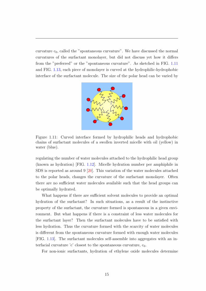
curvature c0, called the ”spontaneous curvature”. We have discussed the normal

curvatures of the surfactant monolayer, but did not discuss yet how it differs

from the ”preferred” or the ”spontaneous curvature”. As sketched in FIG. 1.11

and FIG. 1.13, each piece of monolayer is curved at the hydrophilic-hydrophobic

interface of the surfactant molecule. The size of the polar head can be varied by

Figure 1.11: Curved interface formed by hydrophilic heads and hydrophobicchains of surfactant molecules of a swollen inverted micelle with oil (yellow) inwater (blue).

regulating the number of water molecules attached to the hydrophilic head group

(known as hydration) [FIG. 1.12]. Micelle hydration number per amphiphile in

SDS is reported as around 9 [20]. This variation of the water molecules attached

to the polar heads, changes the curvature of the surfactant monolayer. Often

there are no sufficient water molecules available such that the head groups can

be optimally hydrated.

What happens if there are sufficient solvent molecules to provide an optimal

hydration of the surfactant? In such situations, as a result of the instinctive

property of the surfactant, the curvature formed is spontaneous in a given envi-

ronment. But what happens if there is a constraint of less water molecules for

the surfactant layer? Then the surfactant molecules have to be satisfied with

less hydration. Thus the curvature formed with the scarcity of water molecules

is different from the spontaneous curvature formed with enough water molecules

[FIG. 1.13]. The surfactant molecules self-assemble into aggregates with an in-

terfacial curvature ’c’ closest to the spontaneous curvature, c0.

For non-ionic surfactants, hydration of ethylene oxide molecules determine

15

O

HO OO

O

HO OO

Figure 1.12: Schematic diagram of changing size of the polar region of a non-ionicsurfactant molecule with changing hydration. Blue color represents hydratedwater molecules.

the head group size. Since the solubility of non-ionics are highly dependent on

temperature,’aop’ too depends on temperature. This means that the curvature of

non-ionics has a strong temperature dependence.

1.7 Emulsions

Emulsions are immiscible liquid dispersions stabilised by surfactants. The term

’stabilise’ ranges from a few minutes to years. Depending on the size of the

dispersed particles, emulsions can be classified to

(1) macroemulsion: droplet size from 1.5 - 100 µm

(2) miniemulsion: droplet size from 50 - 500 nm and

(3) microemulsion: droplet size from 3 - 50 nm .

Physical appearance of the emulsion depends on the scattering of light by the

droplets of the dispersed phase. The scattering intensity, I ∼ R6, where R is the

droplet radius. As the droplet diameter decreases, appearance of the emulsions

range from a milky solution or ”macroemulsion” (scatters the entire spectrum of

incident visible light) through a gray translucent solution or ”miniemulsion” (the

droplets are too small to scatter the entire spectrum of incident visible light) and

16

O

HO OO

O

HO OO

Normal curvature Spontaneous curvature

water

water

Rw

oil

Figure 1.13: normal curvature of the surfactant monolayer (less water moleculesto hydrate) and spontaneous curvature of the surfactant monolayer(no constraintof water molecules). Blue and yellow color represents water and oil respectively.

finally to a transparent solution or ”microemulsion” (with droplet diameter less

than the wavelength of the incident visible light).

Despite their structural similarities, microemulsion and macroemulsion dif-

fer substantially in their physical and thermodynamic properties. In the case

of macroemulsions, the diameter of the droplets grows continuously with time,

so that phase separation eventually occurs under gravitational forces; i.e., they

are kinetically stable and their formation requires input of work. In the case

of microemulsions, once the right physio-chemical conditions are achieved, mi-

croemulsification occurs spontaneously; they are thermodynamically stable and

isotropic. Since creaming and flocculations are absent, microemulsions have been

an interest for practical applications [21].

1.8 Microemulsions

Microemulsions, macroscopically homogeneous mixture of water and oil, spon-

taneously forms by the addition of surfactant. The word ”microemulsion” was

originally proposed by Jack H. Schulman in 1959, although the first paper on the

topic dates from 1943 [22, 23, 24, 25, 26].

They are thermodynamically stable and transparent mixtures, in general with

low viscosity. Microscopically they are heterogeneous and form a multitude of

17

structures. The fascinating shapes and forms of microemulsions are related to

the properties of extended (≈ 10..100 m2/cm3) surfactant monolayer at water-

oil interface. Nearly monodisperse droplets, lamellar structure with alternative

layers of water-surfactant and oil-surfactant, cylindrical and sponge like structures

have been observed. They can have unique properties like, ultralow interfacial

tension and the ability to solubilise other immiscible liquids. Their fascinating

thermodynamic and kinetic behavior has been a focus of fundamental research

in the colloid science for the last few decades. A gradual change in temperature

of 10 K can lead to a succession of more than four phase transitions with vastly

different macroscopic properties. For several systems, these morphologies and

the approximate extent of the structures in the phase diagram is known due to

the improved experimental techniques (microscopy, light-, electron- and neutron

scattering, NMR). These improved characterization contributed to the theoretical

and computational modeling of phase diagrams.

1.9 Phase Behavior of Microemulsion

A simple ternary system with water, oil (an alkane) and a non-ionic surfactant

can form a microemulsion at appropriate conditions. The properties and phase

behavior of this system is almost universal for many kind of microemulsion sys-

tems. The temperature and composition dependent phase diagram of microemul-

sion with non-ionic surfactants of type CiEj have been extensively studied by

Kahlweit, Strey, Olsson and co-workers [27, 28, 29]. We have chosen C8E3 and

C4E1 as model surfactants for our investigations due to the well characterised

records of water-alkane-CiEj . Microemulsion have mainly three different macro-

scopic phases which have been systematised, and will be discussed in the following

sections.

1.9.1 Gibbs phase triangle

A Gibbs phase triangle for microemulsions is a ternary phase diagram showing

the phase behavior with changes in the volume fractions of water-oil-surfactant.

This is an empirical visual observation of the system and sometimes neglects a

18

surfactantsurfactant

HH22OO oiloilTαα

Tββ

Figure 1.14: ’Unfolded’ phase prism of water-oil-nonionic surfactant system show-ing the three binary phase diagrams. Shaded portions in figure show the misci-bility gaps.

co-surfactant added to the mixture. Under isobaric conditions, a phase prism can

be constructed with the Gibbs phase triangle water-oil-surfactant taken as the

base of the phase prism and temperature as forth ordinate [see FIG. 1.14].

Unfolding the temperature axis gives three binary systems, water-oil, water-

surfactant and surfactant-oil [2, 30] [see FIG. 1.14]. [Tα is the upper critical

solution temperature (UCST) which is the critical temperature above which the

components are miscible in all proportions. The critical temperature below which

the components of a mixture are miscible for all compositions is the lower critical

solution temperature (LCST) represented here as Tβ]. At lower temperatures all

these three systems show a miscibility gap. A miscibility gap is called the region

in which two phases, with essentially the same structure, have no solubility in

one another or do not mix. The water-oil binary system shows a miscibility gap

over the complete experimental temperature range. The phase diagram for oil-

surfactant mixtures show a lower miscibility gap. Its Tα (UCST) is mostly below

zero degree Celsius. The phase diagram of water- surfactant mixture is more

complicated in comparison with the other two systems. It shows two miscibility

gaps at different temperature with a lower and upper critical points cpβ, cpα at

temperatures Tβ and Tα. The LCST (Tβ) of the upper miscibility loop could

19

probably play a role in the phase behavior of the microemulsion [2].

The schematic phase prism for water-oil-surfactant system with the phase

diagrams at different temperatures is shown in FIG. 1.15.

oiloil

nonnon--ionic surfactantionic surfactant

HH22OO

Tl

Tu

Tβ

cpα

cpβ

Tα

3Φ

Φ2

Φ3

Φ2

Figure 1.15: Schematic phase prism for a water-oil-nonionic surfactant systemwith broken critical lines. Macro-state of the microemulsion sample is sketchedin the left side. For a description see the text. Figure adapted from [2]

.

1Φ- region : The single phase region is a macroscopically homogeneous phase

(Winsor IV) [31]. Here microemulsion solubilises all water and oil. However, the

surfactants self-assemble into different morphologies, depending on the temper-

ature and composition. For example, water droplets in oil, lamellar structure,

bicontinuous, oil droplets in water etc have been observed.

2Φ- region : There are two types of 2Φ- regions. (a) In 2Φ, oil-in-water (o/w)

microemulsions coexists with an oil rich phase where surfactants are only present

as monomers at small concentration (Winsor I)[31]. (b) In 2Φ, water-in-oil (w/o)

microemulsions coexists with a surfactant-poor water phase (Winsor II)[31].

20

3Φ- region : In a three-phase system, a surfactant-rich middle-phase (a mi-

croemulsion phase) coexists with both, a water rich and oil rich phases (Winsor

III or middle-phase microemulsion) [31]).

1.9.2 Fish cut phase diagram

Determination of the entire phase prism is very time consuming. A section

through the phase prism, where the ratio of two components is fixed, and the

composition of the third component and temperature are varied, turned out to be

very useful. As non-ionic microemulsions show a strong temperature-dependent

phase behavior, sections at fixed water to oil ratio have frequently been studied

[FIG. 1.16]. A section through Gibbs phase prism at constant water to oil ratio

and varying non-ionic surfactant concentration is called a ’Fish cut’phase diagram

[FIG. 1.17]. ’Fish cut’ phase diagrams got the name due to its characteristic fish

HH22OO oiloil

TT

NonNon--ionic surfactantionic surfactant

Figure 1.16: Schematic phase prism of water-oil-nonionic surfactant mixture. Theshaded region shows a vertical section with fixed water to oil ratio. microemulsion

like shape [32] [FIG. 1.17]. Often a fish-cut phase diagram is given by volume

fractions. We denote the volume fractions of water, oil and surfactant as φw, φo

and φs respectively. The volume ratio of oil in the mixture of oil and water is ;

αo =φo

φw + φo

The respective volume ratio of surfactant in the mixture is given by

αs =φs

φw + φo + φs

21

lT

uT

TT

sφsφ

Φ2

Φ2

Φ1Φ3

Figure 1.17: Schematic ’fish cut’ phase diagram of a non-ionic microemulsionwith equal water to oil proportion as a function of surfactant concentration. The’body’ of the fish has a surfactant-rich phase coexisting with a water and a oil-rich phase, from a temperature region Tl to Tu (marked with dashed line). The’tail’ of the fish has a single phase region starting from φs towards higher φs.On the either side of the body of the fish, a microemulsion phase coexist with awater-rich or oil-rich phase.

The phase diagram shows the three-phase region floating like a ’fish’ and the

one-phase region forming the ’tail’ of the fish. In a fish cut diagram the 3Φ-region

extends from Tl to Tu. Tl to Tu are the lowest and highest temperature where a

3Φ-region can show up [32]. The temperature (T ) at which ”fish body” intersects

the ”fish tail” is called the phase inversion temperature (PIT) or tricritical point

[33]. The temperature T≈ (Tl + Tu)/2 . For some surfactant-oil-water mixtures,

the phase diagram is symmetric on either side of T . The phase inversion temper-

ature (T ) depends only on the components of the particular microemulsion. The

surfactant concentration at the tricritical point (φs) represents the efficiency of a

surfactant too. It is the minimum amount of surfactant required to completely

emulsify equal amounts of water and oil. In a fish cut diagram at very low concen-

trations, a gap can be formed before the body of the fish (3 phase region). This

is related to the CMC of the surfactant. For long chain surfactants like C12E5,

the 3Φ region starts at a surfactant concentration below 1 wt%, whereas for short

22

chain surfactants like C4E1, the minimum amount of surfactant required to form

a 3Φ microemulsion can be as high as 10 wt%.

The two phase boundaries which make a ’fish’ are named according to the

solvent emulsified. (a) At T ≥ T , across the phase boundary, microemulsion

expels water [2, 34]. Now, a microemulsion phase coexists with a water-rich phase

(2Φ). The phase boundary along which this happens is called water emulsification

boundary [web] and the temperature is denoted by TWEB (φs) [35] . (b) Under

cooling a microemulsion expels oil if T ≤ T . Microemulsion then coexists with

an oil-rich phase (2Φ). The phase boundary along which this happens is called

oil emulsification boundary [oeb] and the temperature dependence is denoted by

TOEB (φs).

On an average, the surfactant monolayer is curved towards oil for T ≤ T

and curved towards water for T ≥ T . As discussed earlier, along T = T , the

morphology of the surfactant monolayer tends to be bicontinuous or lamellar.

This again depends on the concentration of surfactant. At low concentrations,

φs ≤ φs, the surfactant monolayer takes a bicontinuous topology whereas at

high concentrations φs � φs a high viscous lamellar structure can be formed.

Surfactant monolayer takes droplet form when it approaches the phase boundary.

1.9.3 Strong and weak surfactant

Surfactants can be classified according to their ’strength’ in their surface active

properties. In the case of non ionic surfactants of type CiEj, for (i, j) larger than

about (8, 3), the surfactants are considered to have a long chain. They bind

strongly to the interface and are called ’strong surfactants’. They posses a sharp

interfacial profile. Surfactants with (i, j) < (8, 3) posses short chains and hence

attach to the interface in a rather disordered way. Due to the fast exchange of

the surfactant molecules with water and oil, the interface tends to become diffuse

for shorter chain surfactants. These surfactants are termed as weak surfactants.

Example: Pentaethylene glycol monododecyl ether (C12E5) is a strong surfactant

and 2-butoxyethanol (C4E1) is a weak surfactant and triethoxy monooctylether

(C8E3) is a moderate surfactant. The critical micellar concentration (CMC) for

strong surfactant is much lower than for a weak surfactant. Example: CMC of

23

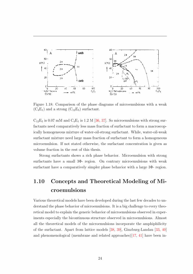
380 Fett/Lipid 101 (1999), Nr. 10, S. 379–388

Fig. 1. Three sections through the phase prism for mixtures of H2O, de-cane, and C4E1. (A) A section for varying mass fraction of surfactantand fixed mass fraction of water and decane (H2O/decane = 50:50). (B)A section for roughly fixed volume fraction of surfactant and varyingmass fraction of decane in decane-plus-water. An extended 3Φ-regionshows up. (C) A section for fixed weight ratio of surfactant (γ = 61wt-%) and varying mass fraction of decane in decane-plus-water. Thewater emulsification boundary (web, upper line) and the oil emulsifica-tion boundary (oeb, lower line) are separated by a homogeneousisotropic single-phase channel 1Φ, connecting the water-rich and theoil-rich side [reproduced from M. Kahlweit und R. Strey, Angew. Chem.97 (1985), 655–669, Fig. 17].

Fig. 2. Three sections through the phase prism for mixtures of H2O,tetradecane, and C12E5. (A) shows a section at equal mass fraction ofwater and tetradecane and varying mass fraction of surfactant. (B) and(C) show sections for constant mass fraction of surfactant and varyingmass fraction of tetradecane in tetradecane-plus-water. Section (B) and(C) differ from each other in that a larger mass fraction of surfactant hasbeen chosen in Fig. 1C, which increases slightly from the left to theright [reproduced from M. Kahlweit und R. Strey, Angew. Chem. 97(1985), 655–669, Fig. 23].

Figure 1.18: Comparison of the phase diagrams of microemulsions with a weak(C4E1) and a strong (C12E5) surfactant.

C12E5 is 0.07 mM and C4E1 is 1.2 M [36, 37]. So microemulsions with strong sur-

factants need comparatively less mass fraction of surfactant to form a macroscop-

ically homogeneous mixture of water-oil-strong surfactant. While, water-oil-weak

surfactant mixture need large mass fraction of surfactant to form a homogeneous

microemulsion. If not stated otherwise, the surfactant concentration is given as

volume fraction in the rest of this thesis.

Strong surfactants shows a rich phase behavior. Microemulsion with strong

surfactants have a small 3Φ- region. On contrary microemulsions with weak

surfactant have a comparatively simpler phase behavior with a large 3Φ- region.

1.10 Concepts and Theoretical Modeling of Mi-

croemulsions

Various theoretical models have been developed during the last few decades to un-

derstand the phase behavior of microemulsions. It is a big challenge to every theo-

retical model to explain the generic behavior of microemulsions observed in exper-

iments especially the bicontinuous structure observed in microemulsions. Almost

all the theoretical models of the microemulsions incorporate the amphiphilicity

of the surfactant. Apart from lattice models [38, 39], Ginzburg-Landau [33, 40]

and phenomenological (membrane and related approaches)[17, 41] have been in-

24

troduced [reviewed in [33]]. The major difference between different models is due

to the variables - microscopic densities in the lattice models, order parameters in

Ginzburg Landau and experimentally accessible parameters in phenomenological

models.

Early papers on microemulsion theories are from Talmon and Prager [42].

They developed a thermodynamical model to describe bicontinuous microemul-

sions. Their approach picturise microemulsions as a random geometry of inter-

spersed oil and water domains (Voronoi polyhedra) with the surfactant adsorbed

at the boundaries. Here, the fluctuations of the monolayers are neglected.

Downloaded 16 Jun 2011 to 194.95.63.248. Redistribution subject to AIP license or copyright; see http://jcp.aip.org/about/rights_and_permissions

Figure 1.19: Oil (shaded) and water (unshaded) domains generated by theVoronoi process. Heavy lines denote the surfactant monolayer

Phenomenological lattice models have been investigated by Ruckenstein

[43] De Gennes and Taupin [44], Jouffroy, Levinson, and De Gennes [45], Widom

[46], Andelman [47] et al. These models employ a lattice parameter ’ξ’ as the

characteristic length scale to calculate the configurational (mixing) entropy of a

microemulsion. The lattice parameter is typically of the order of the dimension

of an oil or a water mesophase.

Talmon and Prager’s model was later modified by de Gennes and coworkers

[44, 45]. They retained the physical content of Talmon and Prager’s model for a

bicontinuous morphology in a simpler picture of regularly packed arrays of cubic

cells as sketched in FIG. 1.20.

These cubic cells are then randomly filled with oil and water. The surfactant

film separates the cells. de Gennes justified his approach by Schulman’s observa-

tion that a bicontinuous phase has a nearly vanishing interfacial tension, γ ≈ 0.

25

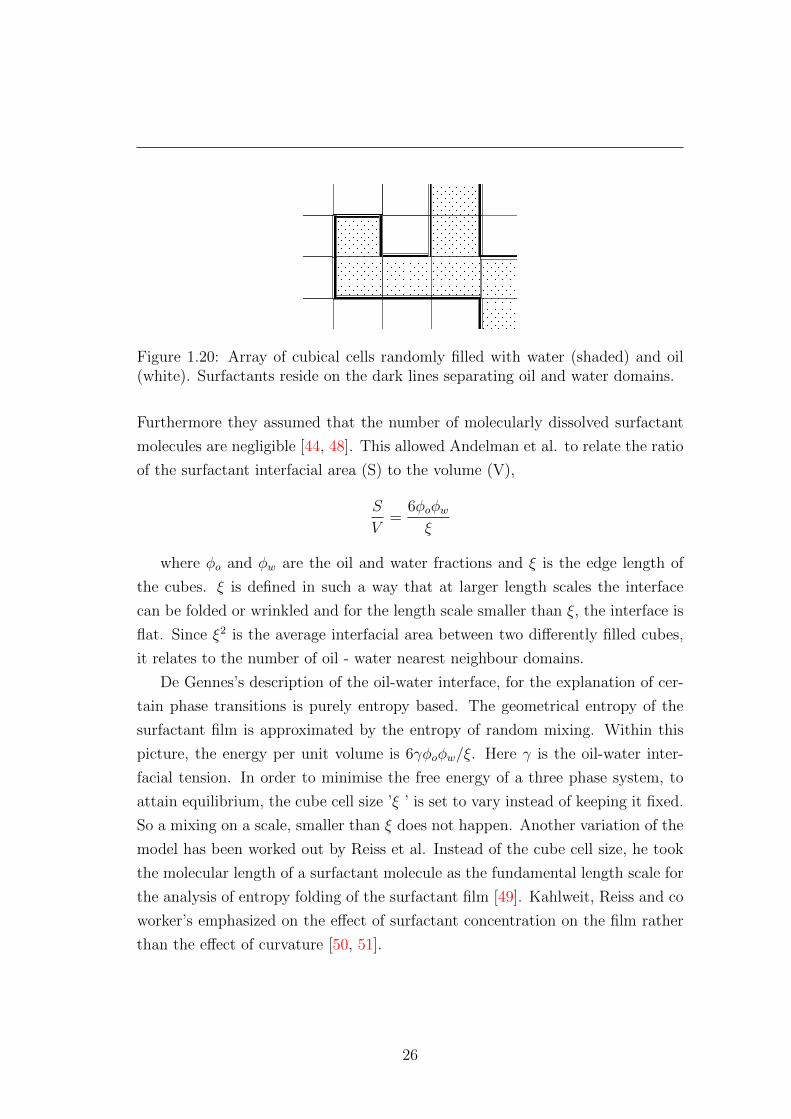
Figure 1.20: Array of cubical cells randomly filled with water (shaded) and oil(white). Surfactants reside on the dark lines separating oil and water domains.

Furthermore they assumed that the number of molecularly dissolved surfactant

molecules are negligible [44, 48]. This allowed Andelman et al. to relate the ratio

of the surfactant interfacial area (S) to the volume (V),

S

V=

6φoφwξ

where φo and φw are the oil and water fractions and ξ is the edge length of

the cubes. ξ is defined in such a way that at larger length scales the interface

can be folded or wrinkled and for the length scale smaller than ξ, the interface is

flat. Since ξ2 is the average interfacial area between two differently filled cubes,

it relates to the number of oil - water nearest neighbour domains.

De Gennes’s description of the oil-water interface, for the explanation of cer-

tain phase transitions is purely entropy based. The geometrical entropy of the

surfactant film is approximated by the entropy of random mixing. Within this

picture, the energy per unit volume is 6γφoφw/ξ. Here γ is the oil-water inter-

facial tension. In order to minimise the free energy of a three phase system, to

attain equilibrium, the cube cell size ’ξ ’ is set to vary instead of keeping it fixed.

So a mixing on a scale, smaller than ξ does not happen. Another variation of the

model has been worked out by Reiss et al. Instead of the cube cell size, he took

the molecular length of a surfactant molecule as the fundamental length scale for

the analysis of entropy folding of the surfactant film [49]. Kahlweit, Reiss and co

worker’s emphasized on the effect of surfactant concentration on the film rather

than the effect of curvature [50, 51].

26

Another class of models are microscopic lattice models. Here lattice points

are considered for analytical convenience but several of these models had the

disadvantage of artifacts. One of the earlier lattice model is from Wheeler and

Widom [52]. They picturized the molecules as difunctional or ’diatomic’ : AA

(oil), BB (water) and AB (surfactant). Like many of the current lattice models,

the configurations of the molecules are restricted in this model also. Here only

the like ends of the molecules meet, so the configuration is uniquely A end or B

end. This makes the model equivalent to a spin 1/2 Ising model, where each site

is uniquely a↑ site or a ↓ site. This earlier model had a draw back of the absence

of a three phase region. This is due to considering only the nearest neighbour

spin-spin interactions leading to one phase and two phase microemulsions.

Later this model has been generalised by including interaction energies, which

gave extremely rich phase diagrams. These generalised models considered further

neighbour sites and three-spin interactions too. Here the free energy of the system

is obtained from the partition function which is again obtained from the sum of

all possible numbers and all possible configurations of AA, BB and AB molecules

(oil, water and surfactant). Similar kind of lattice models have been worked out

by Schick and Shih [38], Robledo [53, 54], Matsen and Sullivan [55]and several

other groups. But none of them could calculate the partition function analyti-

cally even though approximations were made [39]. Among those, ”mean-field”

approximation is most common. The mean-field approximation relates the free

energy F1of a system with Hamiltonian H1 to the free energy F0 of a reference

system with Hamiltonian H0 by

F1 = F0 + <H1 - H0>0

where the probability <>0 of a configuration is weighted with a Boltzmann

factor proportional to exp (-H0/kT). Mean field theories fail to account for the

fluctuations of the surfactant film.

Ginzburg-Landau models is an approach characterised by an expansion in

terms of an order parameter. It can explain many generic aspects of the consid-

ered ternary mixtures including the morphology of the surfactant monolayer close

to phase transitions. This model has a disadvantage of coupling constants which

are are not directly related to physically measured quantities. Due to several

parameters, a quantitative comparison between the result and experiment is also

27

difficult.

Phenomenological (membrane and related approaches) are particulary use-

ful for investigating the phase behavior since the microstructures can be described

via experimentally determined parameters. A description of the interface based

on ’Helfrich energy’ [56, 57, 58] which includes bending rigidities and sponta-

neous curvature (c0) of the interfacial surfactant layer turned out to be successful

in modeling the phase transitions in amphiphilic mixtures.

1.11 Free energy discussions for the non-ionic

microemulsion

The most relevant contributions to the free energy result from (a) the bending

energy of the interface Fb, (b) from the entropy of mixing of water and oil domains

Fmix in a microemulsion phase, and (c) from the undulations of the monolayers

Fu in a lamellar phase. Since the discussions are on non-ionic surfactants, elec-

trostatic contributions to the free energy are irrelevant. The free energy arising

from the bending of an interfacial monolayer was introduced by Helfrich for the

description of lipid bilayers [56]. Later the concept was applied to describe sur-

factant monolayers at the water-oil interface by various authors starting from de

Gennes and Taupin [44]. The free energy per unit area arising from the bending

of the interfacial monolayer is

Fb =κ

2

[ 1

R1

+1

R2

− 2c0

]2

+ κ1

R1R2

(1.7)

Here R1 and R2 are the local radii of curvature. The bending modulus κ

and the Gaussian modulus κ and the spontaneous curvature co(T) are empirical

material constants. The total water-oil interfacial area can be expressed as A/V

=φsls

. Then the free energy per unit volume can be written as,

Fb =φsls

{κ

2

[ 1

R1

+1

R2

− 2c0

]2

+ κ1

R1R2

}(1.8)

Helfrich [56] first calculated the free energy of the lamellar phase, which arises

28

from the steric interaction of undulating lamellar sheets. Fluctuations can have

a major contribution to the free energy. Helfrich’s calculation on the free energy

has been generalized [47] to the specific case of bilayer sheets, so that the free

energy density of the lamellar phase due to undulations is given by,

Fu = (kBT )2χ

κ

φ3s

4l3s

(1

φ2o

+1

φ2w

)1

φo + φw(1.9)

χ is a prefactor with a value approximately 0.05 [47, 59, 60].

Another contribution to the free energy is the different possibilities in dis-

tributing water and oil droplets in space.

Fmix = (kBT )φ3s

6l3sφ3(1− φ)3

[φlogφ+ (1− φ)log(1− φ)

](1.10)

where φ corresponds to the volume fraction of enclosed phase (either water

droplet or oil droplet). The only temperature dependence of this entropy of

mixing is the prefactor kBT. Studies on the temperature dependence of the free

energies per unit volume for single phase mixtures with different morphologies

showed that the contributions to the free energy due to the entropy of mixing Fm

and the undulations of the lamellae Fu are nearly constant within a temperature

interval of 298 K to 320 K [60]. Moreover the values are similar. But the values

for the bending free energies show a strong temperature dependence. For this

reason the contributions to the interfacial free energy per unit volume due to

undulations of the lamellae Fu and due to mixing of water and oil domains Fm

are negligible, for the description of the temperature dependent phase diagrams

and the specific heat of the microemulsion sample.

1.12 Size of droplets

1.12.1 One Phase Region

In the 1Φ- region the size of the droplet is determined by the composition of

the microemulsion. It hardly depends on temperature, therefore its temperature

dependence can be ignored in the following considerations. The size of the droplet

29

can be calculated from the conservation of volume and area.

Here according to the volume conservation,

V · φd = N × 4

3πR3 (1.11)

where N denotes the number of droplets in a volume element V. φd is the enclosed

volume obtained from the sum of the interior volume and the respective oil/water

soluble part of the surfactant. For symmetric surfactants, i.e surfactants where

the volume of the hydrophilic head almost equalises those of the hydrophobic tail,

φd is given by :

φwd = φw +φs2

(1.12)

φod = φo +φs2

(1.13)

According to the area conservation,

Vs · φs = N · 4πR2 · ls (1.14)

ls gives the effective thickness of the surfactant monolayer. From the ratio of

both (13) and (16), the radius of the water droplet is given as

Rw =3lsφdφs

(1.15)

and similarly we get the size of oil droplet as

Ro = −3lsφdφs

(1.16)

To distinguish water and oil droplets, the radius of oil droplet is taken to be

negative.

1.12.2 Two Phase Region

According to Eq.1.15, with increasing volume fraction of water and fixed surfac-

tant concentration, the average size of the droplets should increase. But above

the emulsification boundary (T > TWEB) droplets cannot emulsify all the water.

30

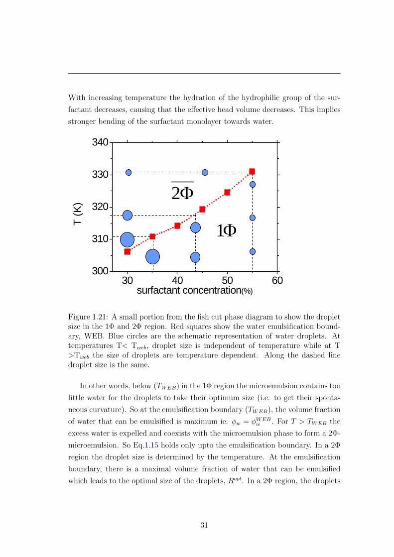
With increasing temperature the hydration of the hydrophilic group of the sur-

factant decreases, causing that the effective head volume decreases. This implies

stronger bending of the surfactant monolayer towards water.

30 40 50 60300

310

320

330

340

T (K

)

surfactant concentration(%)

Φ2

Φ1

Figure 1.21: A small portion from the fish cut phase diagram to show the dropletsize in the 1Φ and 2Φ region. Red squares show the water emulsification bound-ary, WEB. Blue circles are the schematic representation of water droplets. Attemperatures T< Tweb, droplet size is independent of temperature while at T>Tweb the size of droplets are temperature dependent. Along the dashed linedroplet size is the same.

In other words, below (TWEB) in the 1Φ region the microemulsion contains too

little water for the droplets to take their optimum size (i.e. to get their sponta-

neous curvature). So at the emulsification boundary (TWEB), the volume fraction

of water that can be emulsified is maximum ie. φw = φWEBw . For T > TWEB the

excess water is expelled and coexists with the microemulsion phase to form a 2Φ-

microemulsion. So Eq.1.15 holds only upto the emulsification boundary. In a 2Φ

region the droplet size is determined by the temperature. At the emulsification

boundary, there is a maximal volume fraction of water that can be emulsified

which leads to the optimal size of the droplets, Ropt. In a 2Φ region, the droplets

31

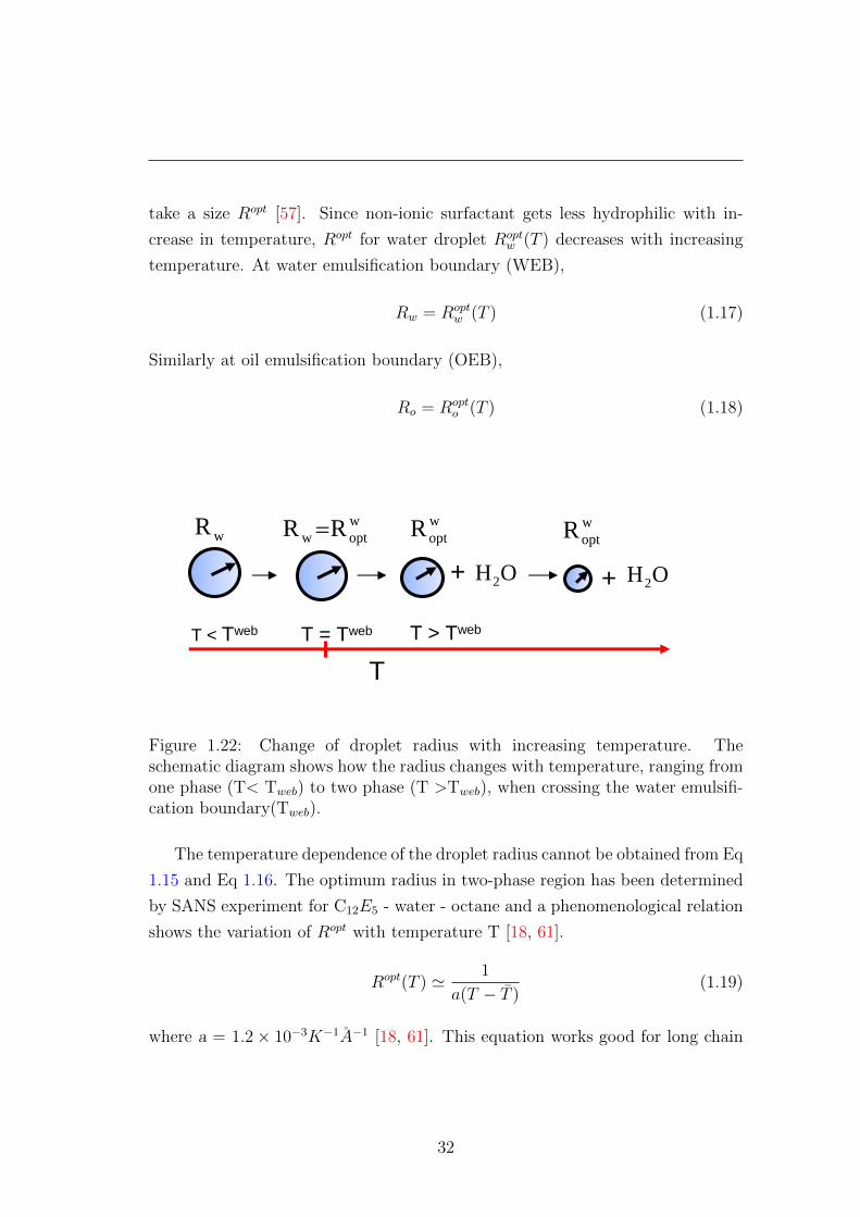
take a size Ropt [57]. Since non-ionic surfactant gets less hydrophilic with in-

crease in temperature, Ropt for water droplet Roptw (T ) decreases with increasing

temperature. At water emulsification boundary (WEB),

Rw = Roptw (T ) (1.17)

Similarly at oil emulsification boundary (OEB),

Ro = Ropto (T ) (1.18)

T < Tweb T = Tweb T > Tweb

T

woptw RR = w

optR

+ OH2 +

woptRwR

OH2

Figure 1.22: Change of droplet radius with increasing temperature. Theschematic diagram shows how the radius changes with temperature, ranging fromone phase (T< Tweb) to two phase (T >Tweb), when crossing the water emulsifi-cation boundary(Tweb).

The temperature dependence of the droplet radius cannot be obtained from Eq

1.15 and Eq 1.16. The optimum radius in two-phase region has been determined

by SANS experiment for C12E5 - water - octane and a phenomenological relation

shows the variation of Ropt with temperature T [18, 61].

Ropt(T ) ' 1

a(T − T )(1.19)

where a = 1.2× 10−3K−1A−1 [18, 61]. This equation works good for long chain

32

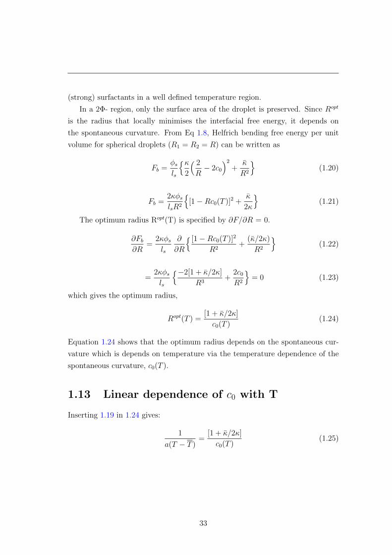
(strong) surfactants in a well defined temperature region.

In a 2Φ- region, only the surface area of the droplet is preserved. Since Ropt

is the radius that locally minimises the interfacial free energy, it depends on

the spontaneous curvature. From Eq 1.8, Helfrich bending free energy per unit

volume for spherical droplets (R1 = R2 = R) can be written as

Fb =φsls

{κ2

( 2

R− 2c0

)2

+κ

R2

}(1.20)

Fb =2κφslsR2

{[1−Rc0(T )]2 +

κ

2κ

}(1.21)

The optimum radius Ropt(T) is specified by ∂F/∂R = 0.

∂Fb∂R

=2κφsls

∂

∂R

{ [1−Rc0(T )]2

R2+

(κ/2κ)

R2

}(1.22)

=2κφsls

{−2[1 + κ/2κ]

R3+

2c0

R2

}= 0 (1.23)

which gives the optimum radius,

Ropt(T ) =[1 + κ/2κ]

c0(T )(1.24)

Equation 1.24 shows that the optimum radius depends on the spontaneous cur-

vature which is depends on temperature via the temperature dependence of the

spontaneous curvature, c0(T ).

1.13 Linear dependence of c0 with T

Inserting 1.19 in 1.24 gives:

1

a(T − T )=

[1 + κ/2κ]

c0(T )(1.25)

33

where κ, κ and ’a’ are material constants. Therefore, to first order,

c0(T ) ∝ (T − T ) (1.26)

where T is the phase inversion temperature or the tricritical point. For strong

surfactants (eg: C12E5) this relation is well established over a temperature region

near to T . But when T � T and T � T the relation cannot be valid any-

more. This is due to the saturation of the spontaneous curvature c0(T ) after the

drop radius decreased so much that it approaches its micellar size. However, an

expression for Roptw (T ) and Ropt

o (T ) is required for the calculation of the tempera-

ture dependence of the emulsification boundaries. This expression should satisfy

certain properties like

1) For sufficiently high temperatures (T � Tl) the size of the water droplets

approaches the inverse micellar size , i. e., Roptw (T ) → Rmic

w

2) For low temperatures (T � Tu) the size of oil droplets approaches the

micellar size, i. e., Ropto (T ) → Rmic

o

3) A prediction of the three phase region.

An expression satisfying all these requirements and leading to good description

of the experimental data is [35]

Roptw (T ) ≡ Rmic

w

1

1− exp(aw(Tl − T ))(1.27)

where Rmicw > 0 and T > Tl and

Ropto (T ) ≡ Rmic

o

1

1− exp(ao(T − Tu))(1.28)

where Rmico < 0 and T < Tu Here Rmic is the micellar radii and aw and ao

characterize the change of the optimal radius with temperature.

34

1.14 Emulsification boundary - 1Φ meets 2Φ re-

gion

At the emulsification boundary R1Φ = Ropt. Now that we have the expressions

for all the radii, insert Eq 1.15 and Eq 1.16 to Eq 1.27 and Eq 1.28 respectively.

exp(aw(Tl − T )) = 1− Rmicw

R1Φw

(1.29)

exp(ao(T − Tu)) = 1− Rmico

R1Φo

(1.30)

Solving this equation for TWEB and TOEB gives the composition dependence of

the emulsification boundaries of water and oil droplets.

TWEB = Tl −1

awln

(1− Rmic

w

3ls

φsφw + xφs

)(1.31)

TOEB = Tu +1

aoln

(1− |R

mico |

3ls

φsφo + (1− x)φs

)(1.32)

These equations imply that the WEB and OEB can be determined from the

material constants in the above equation - the upper and the lower bound of the

3Φ region Tu and Tl respectively, the micellar radii Rmicw and Rmic

o the change

of the optimal radius with temperature aw and ao, the volume fraction of the

hydrophilic head group of a surfactant molecule x and the effective length of the

surfactant ls.

Combining Eq 1.27 and Eq 1.28 with Eq 1.24 yields a generalised expression

for the spontaneous curvature.

cw0 (T ) ≡ [1 + κ/2κ]

Rmicw

1− exp(aw(Tl − T )) (1.33)

co0(T ) ≡ − [1 + κ/2κ]

Rmico

1− exp(ao(T − Tu)) (1.34)

The equations 1.31 and 1.32 gives prediction to emulsification boundaries. If

all the material constants in these equation can determine TWEB and TOEB then

35

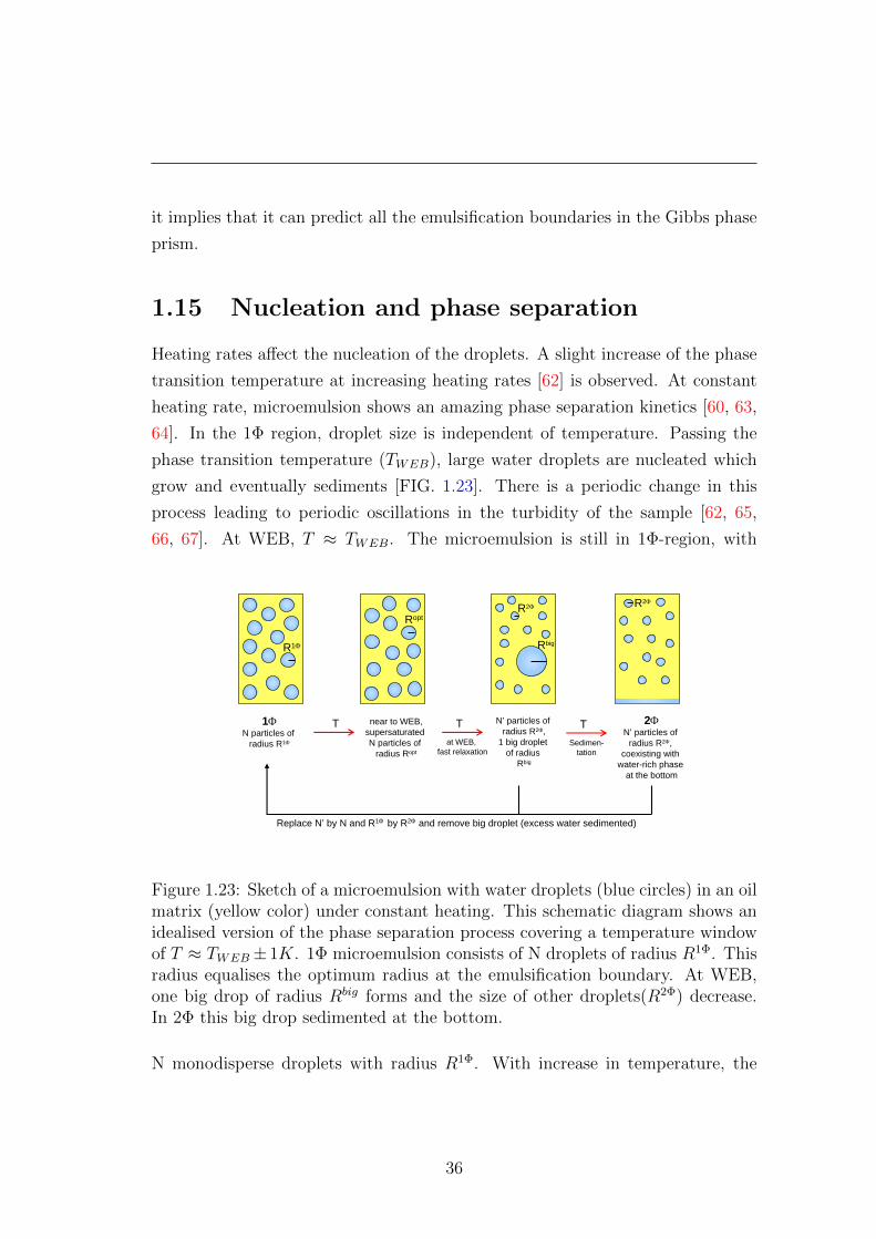
it implies that it can predict all the emulsification boundaries in the Gibbs phase

prism.

1.15 Nucleation and phase separation

Heating rates affect the nucleation of the droplets. A slight increase of the phase

transition temperature at increasing heating rates [62] is observed. At constant

heating rate, microemulsion shows an amazing phase separation kinetics [60, 63,

64]. In the 1Φ region, droplet size is independent of temperature. Passing the

phase transition temperature (TWEB), large water droplets are nucleated which

grow and eventually sediments [FIG. 1.23]. There is a periodic change in this

process leading to periodic oscillations in the turbidity of the sample [62, 65,

66, 67]. At WEB, T ≈ TWEB. The microemulsion is still in 1Φ-region, with

R1Φ

Ropt

R2ΦR2Φ

Rbig

1ΦN particles of

radius R1Φ

near to WEB,supersaturated N particles of

radius Ropt

N’ particles of radius R2Φ,

1 big droplet of radius

Rbig

2ΦN’ particles of

radius R2Φ, coexisting with

water-rich phase at the bottom

T Tat WEB,

fast relaxation

TSedimen-

tation

Replace N’ by N and R1Φ by R2Φ and remove big droplet (excess water sedimented)

Figure 1.23: Sketch of a microemulsion with water droplets (blue circles) in an oilmatrix (yellow color) under constant heating. This schematic diagram shows anidealised version of the phase separation process covering a temperature windowof T ≈ TWEB± 1K. 1Φ microemulsion consists of N droplets of radius R1Φ. Thisradius equalises the optimum radius at the emulsification boundary. At WEB,one big drop of radius Rbig forms and the size of other droplets(R2Φ) decrease.In 2Φ this big drop sedimented at the bottom.

N monodisperse droplets with radius R1Φ. With increase in temperature, the

36

water droplets want to decrease its size. This process is not easy due to the

conservation of area and volume of water and surfactant. On the experimental

time scale, diffusion of water molecules through the oil matrix is negligible. So

the only way to exchange water and surfactant is via collisions [67]. Further

heating of the sample leads to overheating and until it nucleates large droplets,

which take the excess water allowing the majority of the small droplets to attain

their optimum size [see FIG. 1.23]. The number of droplets continuously changes

to conserve the total volume of water and of the area of the internal surface.

These large droplets are energetically ’expensive’ so the system has to pass an

energy barrier before nucleation occurs. Large droplet takes the excess water and

will merge with larger droplets. Further, they sediments to form the water-rich

phase.The amplitude as well as the period of oscillations strongly depend on the

heating rate (νs) as

νs ≡∆T

∆t(1.35)

where T and t are the temperature and the time with which the oscillations peri-

odically varies. These oscillations decay after several periods (nearly 20 periods)

irrespective of the heating rate. A square root dependence of the period on the

heating rate, ∆T ∼ √νs has been reported [62, 68].

1.16 Specific Heat

Since the phase transitions comprise changes of the structure and topology of the

interface between water and oil, an effective free energy for the interface can be

used to describe structural changes in the mixture [18, 19, 57, 58, 60, 69, 70]. The

specific heat ’Cv(T)’ involves the second temperature derivative, hence it probes

the curvature of the free energy.

Cv = T∂S

∂T= −T ∂

2F

∂T 2(1.36)

Bending energy for monodisperse droplets of radius R takes the form,

Fb =2κφslsR2

1Φ

[(1−R1Φc0(T )

)2

+κ

2κ

](1.37)

37

Since the droplet radius in 1Φ (RΦ) is fully determined by the composition, we

can write

R1Φ =3lsφdφs

{≈ 3ls(φw+0.5φs)

φs

≈ −3ls(φo+0.5φs)φs

In two phase region, the droplets can take the preferred size because only the

overall interfacial area has to be conserved. Then the optimum radius is given

by,

|Ropt(T )| =1 + κ

2κ

|co(T )|≤ R1Φ (1.38)

At the emulsification phase boundary ie, from 1Φ and 2Φ, droplet radius R1Φ=

Ropt. Since c0 is the only relevant temperature-dependent parameter [14,18,40],

the specific heat in the 1Φ and 2Φ regions can be obtained. So the specific heat

from 1.36,

C1Φv ≡ −T

∂2F (R1Φ)

∂T 2=−2κφsT

ls

[∂2c2

0(T )

∂T 2− 2

R1Φ

∂2c0(T )

∂T 2

](1.39)

C2Φv ≡ −T

∂2F (Ropt)

∂T 2=−φsTls

[∂2c2

0(T )

∂T 2

]κ

1 + κ2κ

(1.40)

While crossing the phase transition boundary from 1Φ to 2Φ, a step in the

specific heat signal is produced. The height of the signal is denoted by ∆Cstepv ,

which can be obtained by the difference between the specific heats in 1Φ and 2Φ.

∆Cv = C2Φv − C1Φ

v =4κφsT

ls

[∂2c2

0(T )

∂T 2

R1Φ −Ropt

R1ΦRopt

+

(∂c0(T )∂T

)2

11+ κ

2κ

](1.41)

At the emulsification boundary Ropt = R1Φ,

∆Cstepv =

4κφsT

ls

1

1 + κ2κ

(∂c0(T )

∂T

)2

(1.42)

The specific heat is very sensitive to the changes in the curvature of the interface.

This equation gives the information of change in curvature with temperature. So

38

from the change in the specific heat we can probe the curvature details. Since dif-

ferential scanning microcalorimeter measures the temperature-dependent change

of the values for the specific heat, microcalorimetry forms an extremely sensitive

probe of the temperature dependence of the free energies.

39

Chapter 2

Materials and Experimental

Techniques

2.1 Materials

Moderate surfactant: Triethylene glycol mono-n-octyl ether (C8E3) is a colorless

and odourless liquid with molecular formula C14H30O4 and density 0.95 gcm3 at

room temperature.

Weak surfactant: 2-butoxyethanol (C4E1) is a colorless liquid with ether-like

smell. The molecular formula is C6H14O2 and its density is 0.90 gcm3 at room

temperature.

Non-ionic surfactants are purchased from Bachem and used without further

purification (water content). Water is deionised and double distilled with Milli Q

purity with density 0.99 gcm3 at 200C. Decane and Octane (Fluka, Switzerland)

used here have a purity of 99 percentage with densities 0.730 gcm3 and 0.702 g

cm3

respectively.

Sample preparation: The samples are weighed in mass fraction according to

the calculated volume fractions. Glass viols with teflon coated stoppers are used

as sample containers. Sample is weighed with an accuracy of 1 milligram (Mettler

toledo-AB204-S). A magnetic stirring bar was added to each viol to achieve proper

mixing of the sample.

40

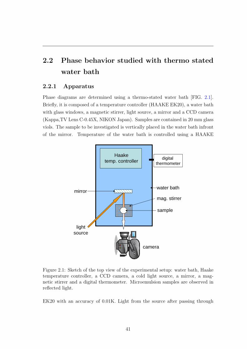
2.2 Phase behavior studied with thermo stated

water bath

2.2.1 Apparatus

Phase diagrams are determined using a thermo-stated water bath [FIG. 2.1].

Briefly, it is composed of a temperature controller (HAAKE EK20), a water bath

with glass windows, a magnetic stirrer, light source, a mirror and a CCD camera

(Kappa,TV Lens C-0.45X, NIKON Japan). Samples are contained in 20 mm glass

viols. The sample to be investigated is vertically placed in the water bath infront

of the mirror. Temperature of the water bath is controlled using a HAAKE

sample

digital thermometer

Haaketemp. controller

light source

mag. stirrer

water bath

camera

mirror

Figure 2.1: Sketch of the top view of the experimental setup: water bath, Haaketemperature controller, a CCD camera, a cold light source, a mirror, a mag-netic stirrer and a digital thermometer. Microemulsion samples are observed inreflected light.

EK20 with an accuracy of 0.01K. Light from the source after passing through

41

a cylindrical lens is directed to the mirror. The reflected light from the mirror

illuminates the sample in the glass viols and the light scattered is captured in a

CCD camera. This CCD is connected with a stereo microscope (NIKON US-3,

Japan) so insitu the phase separation can be observed. The sensor of a digital

thermometer is kept very close to the sample viol to record the temperature

during the experiment.

2.2.2 Procedures to determine phase behavior

The viol containing sample is vertically immersed in a water bath. The sample is

stirred using a magnetic stirring bar to ensure homogeneous mixing. A magnetic

stirrer is placed under the glass vessel containing the water bath, along the ver-

tical axis of the sample viol. The sample undergoes a temperature ramp with a

predefined heating and cooling rate from 1Φ-region to final temperature of phase

separation [TWEB or TOEB]. Simultaneously the temperature is recorded by an

interfaced digital thermometer and the images are also taken.

1Φ microemulsion 2Φ microemulsion 3Φ microemulsion

2 cm

Figure 2.2: Microemulsion samples in 2cm wide viols are observed in reflectedlight. Left: 1Φ microemulsion appears dark due to the complete transmission oflight without any scattering. Center: A 2Φ microemulsion looks turbid due toscattered light by the comparatively big droplets formed during phase separation.Right: In a 3Φ microemulsion, a thin surfactant rich area coexists with an upperoil-rich and a lower water-rich area.

42

Visual inspection of the sample in the scattered light gives three types of

images as shown in FIG. 2.2. Since nanometer sized droplets do not scatter the

white light, an isotropic- 1Φ microemulsion looks dark [FIG. 2.2, left]. From

1Φ-region, sample is heated to 2Φ get TWEB whereas the sample is cooled to 2Φ

to get TOEB. During the temperature ramp, the system passes the emulsification

boundary and bigger droplets are emulsified. These droplets make the sample

turbid by scattering the light [FIG. 2.2, center]. The heating or cooling is stopped

just after the appearence of the turbidity.

A 2Φ microemulsion under stirring appears turbid in the scattered light. Near

to both the phase transition boundaries [TWEB and TOEB], average values are

taken by heating and cooling across each boundary within a temperature win-

dow. TWEB is the temperature of appearence (during heating from 1Φ to 2Φ

) or disappearence (during cooling from 2Φ to 1Φ) of the turbidity. For TOEB,

turbidity appears while cooling from 1Φ to 2Φ and disappears while heating from

2Φ to 1Φ. The values for TWEB and TOEB are averaged out from heating and

cooling of a cycle [FIG. 3.1]. Due to the overheating, the experimental value of

TWEB from a heating cycle is slightly higher than from the cooling cycle.

Both 2Φ and 3Φ microemulsions appear turbid under stirring. Hence the

surfactant rich middle phase in a 3Φ microemulsion is not distinguishable under

stirring. So the phase transition temperatures of 2Φ to 3Φ cannot be determined

with the earlier procedure. Instead undisturbed sample is observed at various

temperatures near to the phase transition temperatures. The temperature is

altered, followed by the stirring of the sample before leaving it undisturbed. De-

pending on the phase separation speed, the sample is kept undisturbed from hours

to several days.

2.3 Differential Scanning Calorimetry

The variation of the specific heat of the solutions as a function of temperature is

measured with a differential scanning calorimeter (VP-DSC, Microcal Inc.).

43

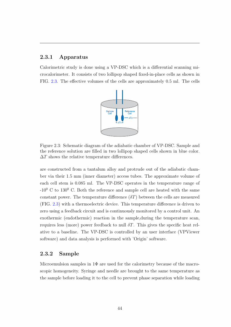
2.3.1 Apparatus

Calorimetric study is done using a VP-DSC which is a differential scanning mi-

crocalorimeter. It consists of two lollipop shaped fixed-in-place cells as shown in

FIG. 2.3. The effective volumes of the cells are approximately 0.5 ml. The cells

Figure 2.3: Schematic diagram of the adiabatic chamber of VP-DSC. Sample andthe reference solution are filled in two lollipop shaped cells shown in blue color.∆T shows the relative temperature differences.

are constructed from a tantalum alloy and protrude out of the adiabatic cham-

ber via their 1.5 mm (inner diameter) access tubes. The approximate volume of

each cell stem is 0.085 ml. The VP-DSC operates in the temperature range of

-100 C to 1300 C. Both the reference and sample cell are heated with the same

constant power. The temperature difference (δT ) between the cells are measured

(FIG. 2.3) with a thermoelectric device. This temperature difference is driven to

zero using a feedback circuit and is continuously monitored by a control unit. An

exothermic (endothermic) reaction in the sample,during the temperature scan,

requires less (more) power feedback to null δT . This gives the specific heat rel-

ative to a baseline. The VP-DSC is controlled by an user interface (VPViewer

software) and data analysis is performed with ’Origin’ software.

2.3.2 Sample

Microemulsion samples in 1Φ are used for the calorimetry because of the macro-

scopic homogeneity. Syringe and needle are brought to the same temperature as

the sample before loading it to the cell to prevent phase separation while loading

44

the cells. After filling the cells are closed as soon as possible for minimising the

contact with air. The air enclosed in the cell might change pressure and volume

during the temperature scan. After filling the reference and the sample cell, the

reference/base line is brought near to 0 cal/0C by adjusting the specific heat via

the amount of water in the reference cell. Double distilled deionized water found

to be an appropriate reference system due to the similar heat capacity.

2.3.3 Procedures to determine the step in the specific

heat

A curve obtained from a calorimetric measurement at a scan rate 5K/h is shown

in FIG. 2.4.

18 21 24 27 30 33

0.000

0.005

0.010

0.015

0.020

Cp(

cal/o C

)

T (oC)

Φ2

Φ2

Φ1baseline

Step 1

Step 2

T1T2

T3

Cp

(cal

/0 C)

rel

Figure 2.4: A DSC curve for water-decane-C8E3 microemulsion of equal volumefraction of water and oil and surfactant volume fraction, φs = 0.31. There are twojumps of the signal: a step at lower temperature T2 due to the oil emulsificationfailure across TOEB (1Φ to underline-2Φ) and the phase transition from 1Φ to 2Φ-overline is identified with a step at higher temperature T1 in the signal (acrossTWEB). The area under the step is shaded. Dashed line shows the baseline inone-phase region.

Here the absolute value for the specific heat is not determined, instead the

specific heat of the microemulsion relative to a baseline set by the water-reference

system is measured. This provides very precise data for the relative specific heat

’Crelv (T)’. The liquid samples (incompressible) do not show significant change in

the volume during phase transition. So we approximate Crelp ≈ Crel

v . Typical

45

heating rates are chosen in the range 7...30 K/h. In FIG. 2.4 two different steps

can be seen at two different temperatures T1 and T2.

The relative specific heat per unit volume is :

Crel(T ) ≡ ∆Q

∆T(2.1)

where ∆Q is the difference between the heat per unit volume absorbed by the

sample and the reference system per temperature increment ∆T. The area under

a step (shaded portion in FIG. 2.4) during the phase transition from 1Φ to 2Φ

allows estimating the heat change ∆Q related to a structural transition

∆Q =

T3∫T1

dT [Crelv (T )− Cbase

v (T )] (2.2)

During a transition, the free energy of bulk water and oil hardly changes. A very

small change of height of baseline after phase transition is due to this.

2.4 Dynamic Light Scattering (DLS)

When light passes through a microemulsion solution, the light will be scattered

due to the Brownian motion of the droplets in the solution. These monodisperse

scatterers are moving randomly in the scattering volume. Hence the density is

fluctuating which leads to intensity fluctuations. The intensity autocorrelation

is the fourier transform of the density autocorrelation. When the scattered light

from two or more scatterers are added together, there will be a position and time

dependent destructive or constructive interference. This leads to time-dependent

fluctuations in the intensity of the scattered light. Dynamic light scattering (DLS)

(Berne, 2000, Pecora, 1985), detects the fluctuations of the scattering intensity

due to the Brownian motion of droplets/molecules in solution to measure the rate

of diffusion of the droplets. The statistics of the scattering signal are analyzed

with a correlator. The data is processed to derive the droplet size where the size is

given by the ”Stokes radius” or ”hydrodynamic radius” of the droplet [FIG. 2.5].

This method has the advantages of short experiment duration and it is almost

46

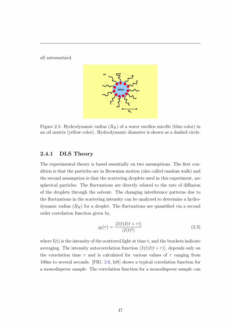
all automatized.

Water

oil

RH

Figure 2.5: Hydrodynamic radius (RH) of a water swollen micelle (blue color) inan oil matrix (yellow color). Hydrodynamic diameter is shown as a dashed circle.

2.4.1 DLS Theory

The experimental theory is based essentially on two assumptions. The first con-

dition is that the particles are in Brownian motion (also called random walk) and

the second assumption is that the scattering droplets used in this experiment, are

spherical particles. The fluctuations are directly related to the rate of diffusion

of the droplets through the solvent. The changing interference patterns due to

the fluctuations in the scattering intensity can be analyzed to determine a hydro-

dynamic radius (RH) for a droplet. The fluctuations are quantified via a second

order correlation function given by,

g2(τ) =〈I(t)I(t+ τ)〉〈I(t)2〉

(2.3)

where I(t) is the intensity of the scattered light at time t, and the brackets indicate

averaging. The intensity autocorrelation function 〈I(t)I(t+ τ)〉, depends only on

the correlation time τ and is calculated for various values of τ ranging from

100ns to several seconds. [FIG. 2.6, left] shows a typical correlation function for

a monodisperse sample. The correlation function for a monodisperse sample can

47

Normalised intensity correlation function

0.0 2.0x10-4 4.0x10-4 6.0x10-4 8.0x10-4 1.0x10-30

5

10

15

20

25

Γ Linear Fit

Γ (m

s-1)

q2 (nm-2)

10-5 10-4 10-3 10-2 10-1 100 101 102 103 104 105 106 107-0.1

0.0

0.1

0.2

0.3

0.4

0.5

0.6

0.7

0.8

0.9

1.0

Lag Time [ms]

β

B

Figure 2.6: Left: The exponentially decaying autocorrelation function (greenline). Right: Decay rate versus scattering vector at different scattering angles(black triangle) with a linear fit (red line).

be analyzed by the equation

g2(τ) = B + βexp(−2Γτ). (2.4)

where B is the baseline of the correlation function at infinite delay (dashed lines

in FIG. 2.6 left), β is the correlation function amplitude at zero delay (dotted

line in FIG. 2.6 left), and Γ is the decay rate. This measured correlation function

is fitted using a regularised fit (ALV-Correlator software V.3.0) to retrieve the

decay rate Γ. It is related to the diffusion coefficient using the relation [FIG. 2.6

right],

D =Γ

q2(2.5)

where q is the magnitude of the scattering vector [FIG. 2.7]. It is given by,

q =4πn

λsin(θ/2) (2.6)

where n is the refractive index of the solvent, λ is the wavelength of the incident

light, and θ is the scattering angle.

The Stokes- Einstein-equation may be used to convert the measured diffusion

48

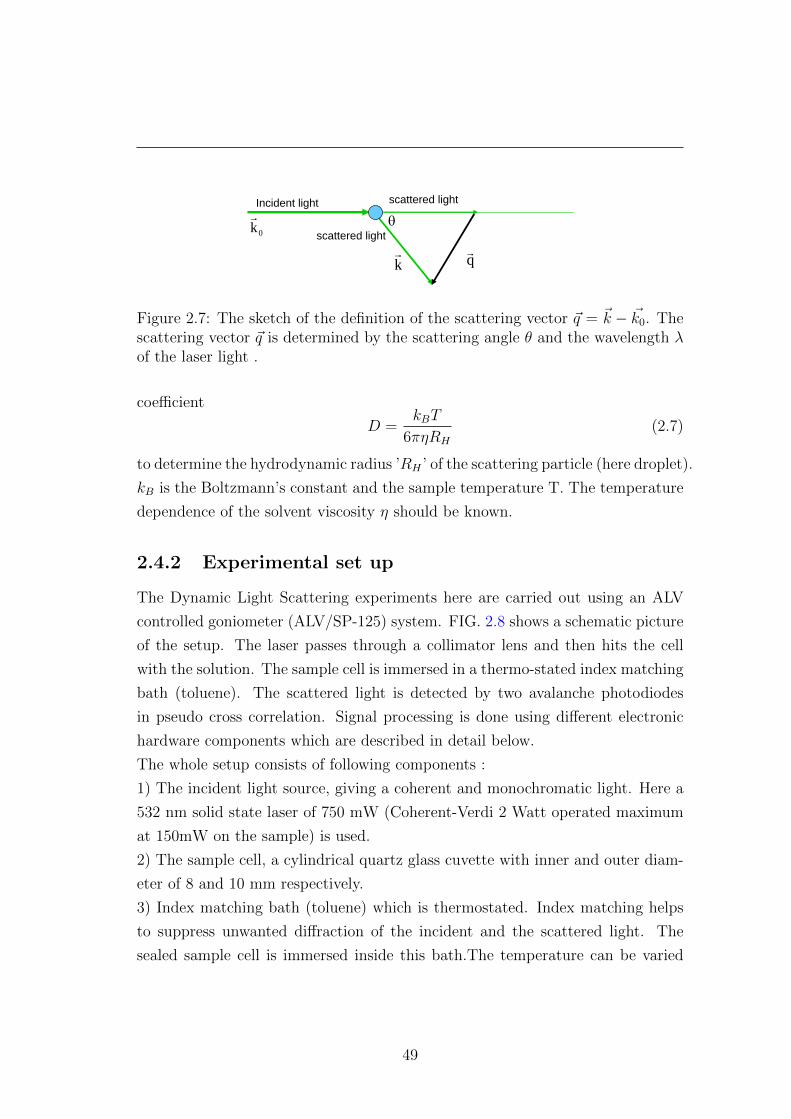
θ0kr

kr qr

Incident light scattered light

scattered light

Figure 2.7: The sketch of the definition of the scattering vector ~q = ~k − ~k0. Thescattering vector ~q is determined by the scattering angle θ and the wavelength λof the laser light .

coefficient

D =kBT

6πηRH

(2.7)

to determine the hydrodynamic radius ’RH ’ of the scattering particle (here droplet).

kB is the Boltzmann’s constant and the sample temperature T. The temperature

dependence of the solvent viscosity η should be known.

2.4.2 Experimental set up

The Dynamic Light Scattering experiments here are carried out using an ALV

controlled goniometer (ALV/SP-125) system. FIG. 2.8 shows a schematic picture

of the setup. The laser passes through a collimator lens and then hits the cell

with the solution. The sample cell is immersed in a thermo-stated index matching

bath (toluene). The scattered light is detected by two avalanche photodiodes

in pseudo cross correlation. Signal processing is done using different electronic

hardware components which are described in detail below.

The whole setup consists of following components :

1) The incident light source, giving a coherent and monochromatic light. Here a

532 nm solid state laser of 750 mW (Coherent-Verdi 2 Watt operated maximum

at 150mW on the sample) is used.

2) The sample cell, a cylindrical quartz glass cuvette with inner and outer diam-

eter of 8 and 10 mm respectively.

3) Index matching bath (toluene) which is thermostated. Index matching helps

to suppress unwanted diffraction of the incident and the scattered light. The

sealed sample cell is immersed inside this bath.The temperature can be varied

49

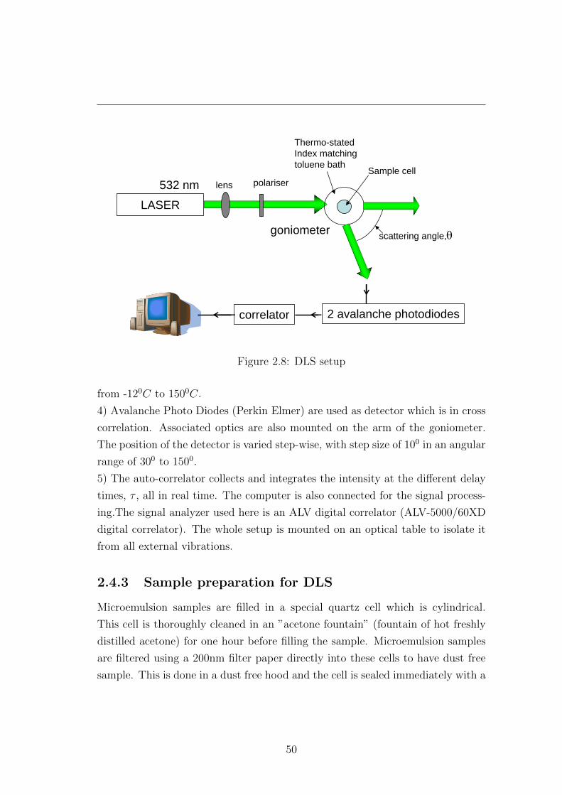
LASER

goniometer

Sample cell

Thermo-stated Index matchingtoluene bath

532 nm

2 avalanche photodiodescorrelator

scattering angle,θ

lens polariser

Figure 2.8: DLS setup

from -120C to 1500C.

4) Avalanche Photo Diodes (Perkin Elmer) are used as detector which is in cross

correlation. Associated optics are also mounted on the arm of the goniometer.

The position of the detector is varied step-wise, with step size of 100 in an angular

range of 300 to 1500.

5) The auto-correlator collects and integrates the intensity at the different delay

times, τ , all in real time. The computer is also connected for the signal process-

ing.The signal analyzer used here is an ALV digital correlator (ALV-5000/60XD

digital correlator). The whole setup is mounted on an optical table to isolate it

from all external vibrations.

2.4.3 Sample preparation for DLS

Microemulsion samples are filled in a special quartz cell which is cylindrical.

This cell is thoroughly cleaned in an ”acetone fountain” (fountain of hot freshly

distilled acetone) for one hour before filling the sample. Microemulsion samples

are filtered using a 200nm filter paper directly into these cells to have dust free

sample. This is done in a dust free hood and the cell is sealed immediately with a

50

teflon tape. Microemulsion samples are sensitive to temperature so they are kept

in the toluene bath for nearly 3 hours to equilibrate (1 phase samples). 2 phase

samples are kept for longer duration (nearly 12 hours to 24 hours) to ensure that

they reached thermodynamic equilibrium before measurement. While filtering

some sample is lost due to filter paper. In case of 2-phase samples, this leads

to an error and repeated measurement is required in that case to get an average

good data.

2.5 Tensiometry

2.5.1 Critical Micelle Concentration (CMC)

Up to CMC the surface tension of water reduces significantly due to surfactant

molecules at surface. Due to saturation, surface tension is constant above CMC.

So measurement of the surface tension of the surfactant solutions is a principal

method to determine the CMC.

Surface tension of a liquid is due to the cohesive interactions with neighboring

molecules. In order to increase the surface area, mechanical work is required. So

surface tension can be defined as the surface work dW required to increase the

surface area A by dA. It can be viewed as a force exerted per unit length [mN/m].

Surfactant solutions exhibit a specific surface tension curve against concentration

as shown in a schematic figure given below [FIG. 2.9].

From pure liquid up to a micellar solution the surface tension decreases linearly

with the logarithm of surfactant concentration. Due to constant surface tension of

the sample from CMC onwards, a kink is formed. The concentration at this kink

is taken as the CMC. The measurement of surface tension (air-liquid interface)

is based on force measurement. A probe is hung on a balance and brought into

contact with the liquid surface. The balance experience a force, as the probe touch

the liquid surface. These forces depend on many factors like the size and shape

of the probe, the contact angle of the probe-liquid interaction and the surface

tension of the liquid. The size and shape of the probe are easy to control. The

du Nouy ring and Wilhelmy plate are mostly used probes ( FIG. 2.10). We used

a DCAT 11EC tensiometer from dataphysics for determining CMC. Tensiometer

51

Figure 2.9: Kink formation due to micelle formation showed by the surface tensionagainst concentration curve obtained from a tensiometer experiment.

is interfaced and works on weight based measurements.

2.5.2 Wilhelmy Plate method

Wilhelmy Plate method is used for measuring surface tension here. The thin plate

is oriented perpendicular to the sample using a balance [FIG. 2.10]. The liquid

sample is raised until the contact with the plate is registered. At the moment of

contact, the balance experience maximum tension. Tension is calculated as,

γwplateair−water =FmaxL. cos θ

(2.8)

where γwplateair−water = surface tension, Fmax= force acting on the balance, L=wetted

length in mm and θ = contact angle. The plate is made of roughened platinum

(high-energy surface) to get virtual zero contact angle. Then cos θ has a value of

approximately 1. Then only the measured force Fmax and the wetted length of

the plate need to be taken into consideration. The surfactant concentration series

is generated automatically with a computer-controlled Liquid Dispensing Unit

(LDU). Experiment starts with pure liquid and then an increasing concentration

method is done using the LDU. For a concentrated sample, approximately 4 times

CMC is used. This concentrated sample is dispensed at constant volume (0.5ml)

using LDU at constant intervals. The measurements and their evaluation are

carried out automatically.

52

θliquidliquid

air

(a) du Noüy ring (b) Wilhelmy plate

F

Figure 2.10: (a) Schematic diagram of du Nouy ring. The ring registers thecontact with the liquid surface and is pushed through the liquid surface to a fewmillimeters down. Then it is pulled up until the maximum Force is reached. (b)Schematic diagram of a Wilhelmy plate during surface tension measurement. Theplate is wetted by a length l and makes an angleθ with the liquid surface. A forceF acts due to the contact with liquid.

2.5.3 du Nouy ring method

Another technique to measure surface tension using tensiometer is the du Nouy

ring method [71] [FIG. 2.10]. Unlike the plate method, this method hardly affects

the wetting properties. A du- Nouy ring is a platinum-iridium ring. This ring is

attached to the balance after cleaning thoroughly with flame. Then it is lowered

beneath the liquid surface.

The surface tension is measured by pulling the ring upward. The ring raises

with a liquid meniscus. Maximum force required to break the ring free of the

liquid meniscus is measured and this force is related to liquid’s surface tension as

follows.

γringair−water =Fmax4πr

(2.9)

where γringair−water= surface tension; Fmax= maximum force and r = radius of the

ring. The contact angle goes to zero at maximum force. Due to the difference of

the inner and outer diameter of the ring the maximum force experienced needs a

53

correction. Here the Harkins Jordan correction factor is used.

54

Chapter 3

Experimental Results and

Discussions

3.1 Phase Behaviour

Phase diagrams are determined for the non-ionic microemulsions with surfac-

tants C8E3 and C4E1, following the procedures from the Section XV.B. Data

from the optical measurement (appearance and disappearance of the turbidity)

are discussed here. The averaged out values from the cooling and heating cycle

is taken for water emulsification boundary (TWEB) as well as for the oil emulsi-

fication boundary (TOEB). Data for four different surfactant concentrations for

a 1:1 water-oil microemulsion are shown in FIG. 3.1 as an example. Due to the

nucleation of the droplets just before phase separation, overheating of the sample

leads to a slight higher temperature for TWEB on a heating cycle. A difference

of 0.1K to 0.9K between cooling and heating is observed for TWEB. For 60%

surfactant concentration, TWEB for cooling is slightly higher than the heating.

This could be due to the evaporation of the water molecules at 328K which later

condensed at the lid of the viol, changing the concentration of the microemulsion

thereby TWEB too.

55

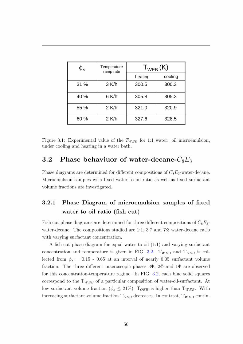
320.9321.02 K/h55 %

328.5327.62 K/h60 %

6 K/h

3 K/h

Temperature ramp rate

305.3305.840 %

300.3300.531 %

TWEB (K)φsheating cooling

Figure 3.1: Experimental value of the TWEB for 1:1 water: oil microemulsion,under cooling and heating in a water bath.

3.2 Phase behaviuor of water-decane-C8E3

Phase diagrams are determined for different compositions of C8E3-water-decane.

Microemulsion samples with fixed water to oil ratio as well as fixed surfactant

volume fractions are investigated.

3.2.1 Phase Diagram of microemulsion samples of fixed

water to oil ratio (fish cut)

Fish cut phase diagrams are determined for three different compositions of C8E3-

water-decane. The compositions studied are 1:1, 3:7 and 7:3 water-decane ratio

with varying surfactant concentration.

A fish-cut phase diagram for equal water to oil (1:1) and varying surfactant

concentration and temperature is given in FIG. 3.2. TWEB and TOEB is col-

lected from φs = 0.15 - 0.65 at an interval of nearly 0.05 surfactant volume

fraction. The three different macroscopic phases 3Φ, 2Φ and 1Φ are observed

for this concentration-temperature regime. In FIG. 3.2, each blue solid squares

correspond to the TWEB of a particular composition of water-oil-surfactant. At

low surfactant volume fraction (φs ≤ 21%), TOEB is higher than TWEB. With

increasing surfactant volume fraction TOEB decreases. In contrast, TWEB contin-

56

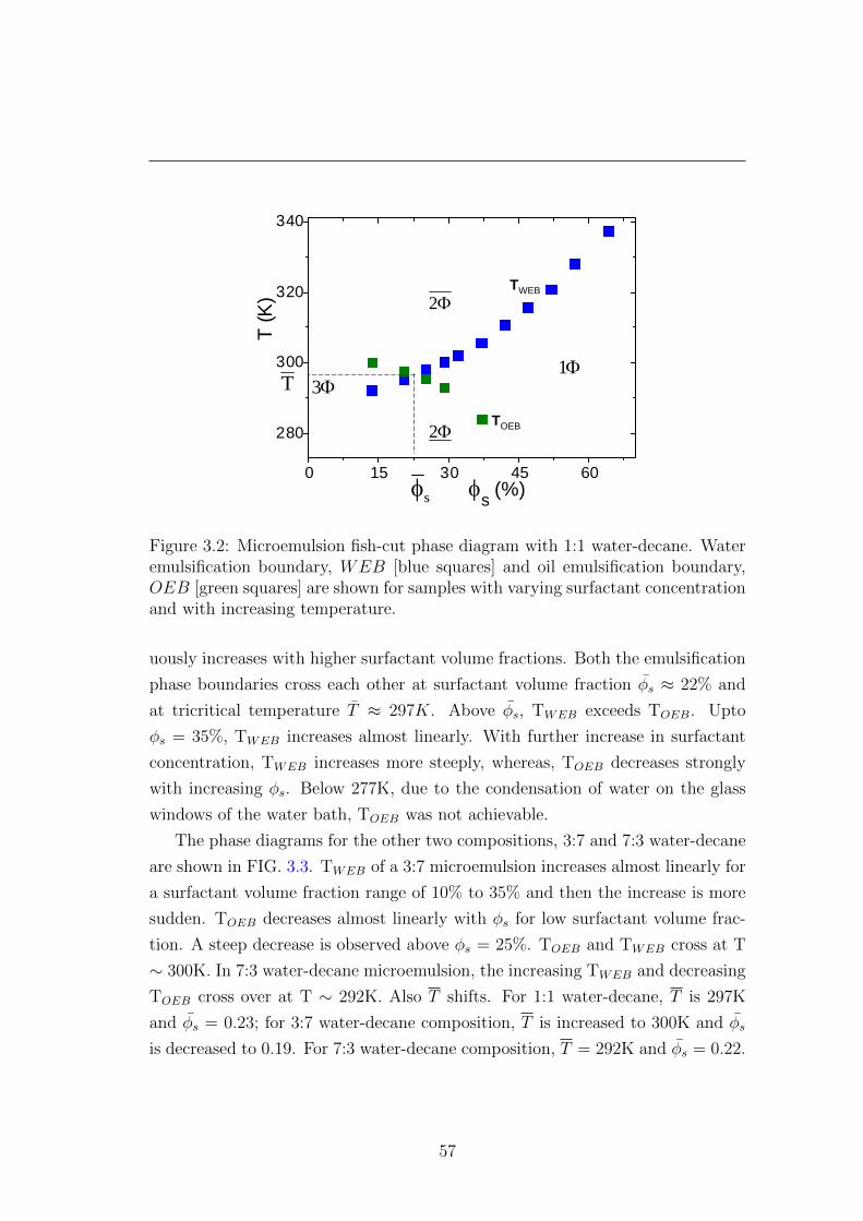
0 15 30 45 60

280

300

320

340

φs (%)

T (K

)

T

sφ

Φ2

Φ2

Φ1Φ3

TWEB

TOEB

Figure 3.2: Microemulsion fish-cut phase diagram with 1:1 water-decane. Wateremulsification boundary, WEB [blue squares] and oil emulsification boundary,OEB [green squares] are shown for samples with varying surfactant concentrationand with increasing temperature.

uously increases with higher surfactant volume fractions. Both the emulsification

phase boundaries cross each other at surfactant volume fraction φs ≈ 22% and

at tricritical temperature T ≈ 297K. Above φs, TWEB exceeds TOEB. Upto

φs = 35%, TWEB increases almost linearly. With further increase in surfactant

concentration, TWEB increases more steeply, whereas, TOEB decreases strongly

with increasing φs. Below 277K, due to the condensation of water on the glass

windows of the water bath, TOEB was not achievable.

The phase diagrams for the other two compositions, 3:7 and 7:3 water-decane

are shown in FIG. 3.3. TWEB of a 3:7 microemulsion increases almost linearly for

a surfactant volume fraction range of 10% to 35% and then the increase is more

sudden. TOEB decreases almost linearly with φs for low surfactant volume frac-

tion. A steep decrease is observed above φs = 25%. TOEB and TWEB cross at T

∼ 300K. In 7:3 water-decane microemulsion, the increasing TWEB and decreasing

TOEB cross over at T ∼ 292K. Also T shifts. For 1:1 water-decane, T is 297K

and φs = 0.23; for 3:7 water-decane composition, T is increased to 300K and φs

is decreased to 0.19. For 7:3 water-decane composition, T = 292K and φs = 0.22.

57

0 15 30 45 60280

300

320

340

T (K

)

φs(%)

TWEB

TOEB

7:3

3:7

T3:7

T7:3

φ7:3φ3:7

Φ1

Figure 3.3: Microemulsion phase diagram with 3:7 (black squares) and 7:3 (greentriangles) water-decane. TWEB [solid symbols] and TOEB [open symbols] areshown for microemulsion samples with increasing surfactant concentration.

The fish-cut moves upwards with decrease in water to water-oil proportion (3:7)

while the emulsification temperatures decreases with an increase in the water to

water-oil ratio (7:3).

3.2.2 Phase Diagram of samples with fixed Surfactant Con-

centration

The effect of surfactant on the microemulsion system is investigated by fixing the

surfactant volume fraction and varying oil to oil + water ratios (αo). Such a cut

along the phase prism is sketched in the inset of FIG. 3.4, known as Shinoda cut

[72, 73].

In FIG. 3.4, the water and oil emulsification boundaries are investigated for

three different microemulsion samples with fixed surfactant volume fraction (φs)

as a function of αo. TWEB is investigated for φs = 35% (green solid circles in

FIG. 3.4), 40% (blue solid circles) and 50% (orange solid circles). The narrow

1φ-region extends over the entire temperature regime and αo. In 1φ-region, at

low temperatures and a low oil to oil plus water ratio (αo) the mixture takes bi-

58

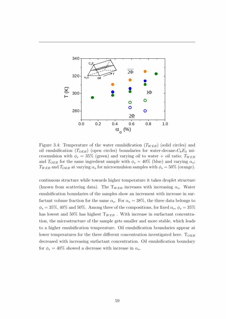
0.0 0.2 0.4 0.6 0.8 1.0

280

300

320

340

T (K

)

αo (%)

HH22OO oiloilTT

CC88EE33

Φ2

Φ1

Φ2

Figure 3.4: Temperature of the water emulsification (TWEB) (solid circles) andoil emulsification (TOEB) (open circles) boundaries for water-decane-C8E3 mi-croemulsion with φs = 35% (green) and varying oil to water + oil ratio; TWEB

and TOEB for the same ingredient sample with φs = 40% (blue) and varying αo;TWEB and TOEB at varying αo for microemulsion samples with φs = 50% (orange).

continuous structure while towards higher temperature it takes droplet structure

(known from scattering data). The TWEB increases with increasing αo. Water

emulsification boundaries of the samples show an increment with increase in sur-

factant volume fraction for the same αo. For αo = 38%, the three data belongs to

φs = 35%, 40% and 50%. Among three of the compositions, for fixed αo, φs = 35%

has lowest and 50% has highest TWEB . With increase in surfactant concentra-

tion, the microstructure of the sample gets smaller and more stable, which leads

to a higher emulsification temperature. Oil emulsification boundaries appear at

lower temperatures for the three different concentration investigated here. TOEB

decreased with increasing surfactant concentration. Oil emulsification boundary

for φs = 40% showed a decrease with increase in αo.

59

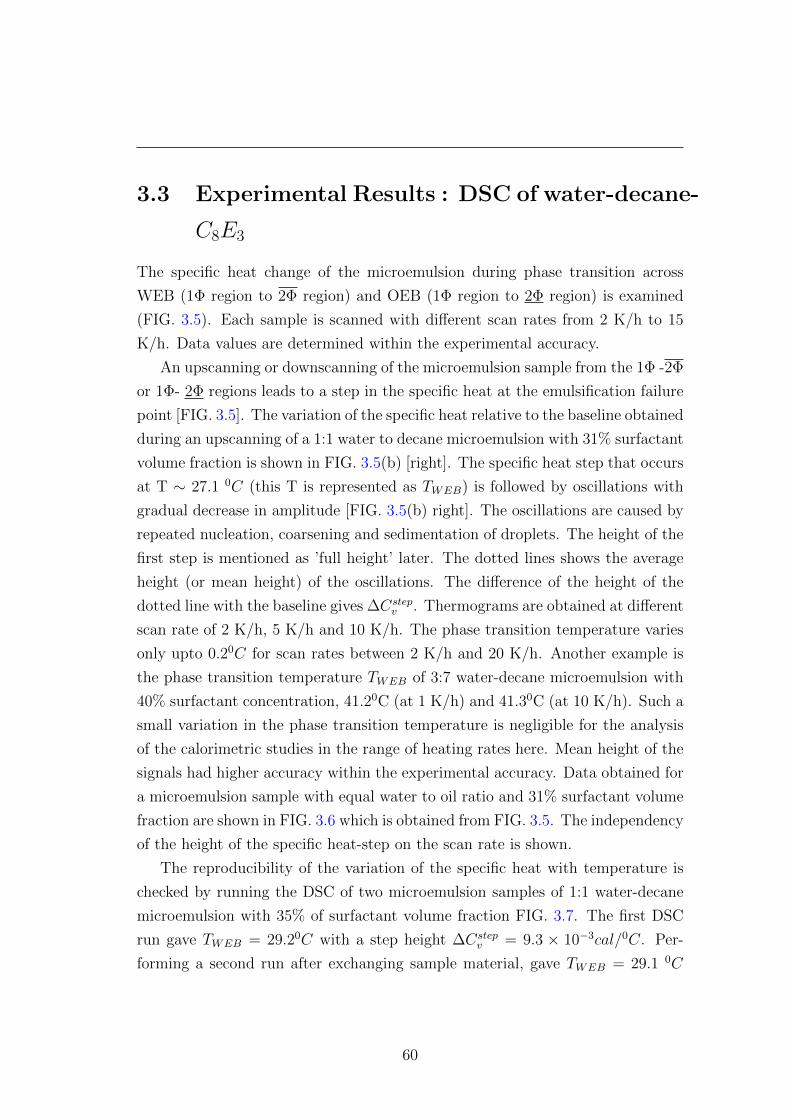
3.3 Experimental Results : DSC of water-decane-

C8E3

The specific heat change of the microemulsion during phase transition across

WEB (1Φ region to 2Φ region) and OEB (1Φ region to 2Φ region) is examined

(FIG. 3.5). Each sample is scanned with different scan rates from 2 K/h to 15

K/h. Data values are determined within the experimental accuracy.

An upscanning or downscanning of the microemulsion sample from the 1Φ -2Φ

or 1Φ- 2Φ regions leads to a step in the specific heat at the emulsification failure

point [FIG. 3.5]. The variation of the specific heat relative to the baseline obtained

during an upscanning of a 1:1 water to decane microemulsion with 31% surfactant

volume fraction is shown in FIG. 3.5(b) [right]. The specific heat step that occurs

at T ∼ 27.1 0C (this T is represented as TWEB) is followed by oscillations with

gradual decrease in amplitude [FIG. 3.5(b) right]. The oscillations are caused by

repeated nucleation, coarsening and sedimentation of droplets. The height of the

first step is mentioned as ’full height’ later. The dotted lines shows the average

height (or mean height) of the oscillations. The difference of the height of the

dotted line with the baseline gives ∆Cstepv . Thermograms are obtained at different

scan rate of 2 K/h, 5 K/h and 10 K/h. The phase transition temperature varies

only upto 0.20C for scan rates between 2 K/h and 20 K/h. Another example is

the phase transition temperature TWEB of 3:7 water-decane microemulsion with

40% surfactant concentration, 41.20C (at 1 K/h) and 41.30C (at 10 K/h). Such a

small variation in the phase transition temperature is negligible for the analysis

of the calorimetric studies in the range of heating rates here. Mean height of the

signals had higher accuracy within the experimental accuracy. Data obtained for

a microemulsion sample with equal water to oil ratio and 31% surfactant volume

fraction are shown in FIG. 3.6 which is obtained from FIG. 3.5. The independency

of the height of the specific heat-step on the scan rate is shown.

The reproducibility of the variation of the specific heat with temperature is

checked by running the DSC of two microemulsion samples of 1:1 water-decane

microemulsion with 35% of surfactant volume fraction FIG. 3.7. The first DSC

run gave TWEB = 29.20C with a step height ∆Cstepv = 9.3 × 10−3cal/0C. Per-

forming a second run after exchanging sample material, gave TWEB = 29.1 0C

60

lT

uTT

sφ

Φ2

Φ2

Φ1Φ3

TOEB

TWEB

(a)

24 26 28 30 32

0.00

0.01

0.02

0.03

ΔCv(c

al/o C

)

T (oC)18 19 20 21

0.00

0.01

ΔCv(c

al/o C

)

T (oC)

downscanning across TOEB upscanning across TWEB

ΔCstep

ΔCstep

5 K/h

2 K/h2 K/h

ΔCstep

ΔCstep5 K/h

TTWEBWEBTTOEBOEB

v

v

v

v

(b)

Φ2 Φ1 Φ1 Φ2

(full height)

(mean height)

Figure 3.5: (a) The schematic fish cut phase diagram with the temperature line(red color arrows) along which calorimetry is done. Red arrows show the direc-tion and the temperature intervals investigated by calorimetry. A sketch of 1Φmicroemulsions (water droplets in oil or oil droplets in water) to the overline−2Φor underline−2Φ microemulsion (microemulsion with water or oil droplets coex-isting with expelled water or oil) is shown. (b) A step in the specific heat signal(solid squares) when passing TWEB during an upscanning from 1Φ region to theoverline − 2Φ region (right). Data taken at a scan speed of 2 K/h (pink) and5 K/h (yellow) are shown. The average height of the step is given by the ar-rows. Solid lines denote the baseline in the 1Φ region and the dashed lines showsthe baseline in the 2Φ region. While downscanning, the specific heat shows astep when passing the oil emulsification boundary (left Fig. with open squares).The data plot at 2K/h is shifted along the y-axis in both figures for better eyeguidance.

61

0.002

0.002

ΔCVSTEP

(cal/ 0C)[1Φ to 2Φ]

19.40.00827.15 0C/h

19.40.00727.02 0C/h

TOEB

(0C)ΔCV

STEP

(cal/ 0C)[1Φ to 2Φ]

TWEB

(0C)Up / down scan rate

Figure 3.6: Analysed DSC data for microemulsions with 1:1 water : oil and 31%of surfactant volume fraction. ∆Cstep

v while crossing WEB and OEB, at twodifferent scan rates, hardly depend on scan rate within experimental accuracy.TWEB and TOEB are also recorded.

with a step height ∆Cstepv = 9.7× 10−3cal/0C. Fresh samples were used for both

the runs. Note that ∆Cstepv is reproducible within very high accuracy.

The variation of the height of the step with φs is shown in FIG. 3.8, FIG. 3.9

and FIG. 3.10 for the three different ratios of water to oil. Height of the full step

(solid symbol) and the mean height (open symbol) are recorded. Eventhough the

absolute values are different for full step height and mean height, the trend of the

specific heat steps are the same for both sets of data.

For 1:1 water-decane ratio (FIG. 3.8), the phase transition temperatures TWEB

increases from 300K to 326K if surfactant concentration (φs) increases from 31%

to 60%. With increasing TWEB, an increase in the step height is observed upto

TWEB ∼ 326K [FIG. 3.8]. The last three data points shows almost the same

height.

For 3:7 water-decane ratio, initially ∆Cstepv increases with increasing TWEB

[FIG. 3.9] and passes a maximum value at TWEB ∼ 320K. This indicates that

with increasing surfactant concentration, the step height increases and drops after

reaching a maximum value. The temperature TWEB ∼ 320K could be of interest

in further studies in understanding the mechanism of the system. [how to relate

this non-monotonic trend of steps in specific heat with the phase transition in

the microemulsion which is not visible in the phase diagram]. For bigger domain

62

TTWEBWEB

26 28 30 32 34 360.000

0.003

0.006

0.009

0.012

0.015

Cp(

cal/o C

)

Temperature (oC)

Figure 3.7: DSC data for microemulsion sample with 1:1 water:oil and 35% ofsurfactant volume fraction. Experiments are done at 1.4 K/h. ∆Cstep

v whilecrossing WEB is obtained with an accuracy of 0.01 cal/0C. The TWEB showed areproducibility with an accuracy of 0.1 0C. The mean height of the step is shownby dotted and dashed lines.

sizes as well as for small domain sizes, the step height is less than that for the

intermediate ones. The effect of the changed solubility of surfactant in the water

and decane may also effect the step height at high temperatures. The max.step

height ∆Cstepv of 3:7 water-oil ratio microemulsion is reduced by nearly 1 mcal/0C

compared to the maximal step height of 1:1 water-oil ratio microemulsion.

The third sample, 7:3 water-decane microemulsion also showed an increase of

∆Cstepv with increasing surfactant concentration [FIG. 3.10]. The data points cor-

respond to φs from 35% to 55%. For this sample, ∆Cstepv increases monotonically

with surfactant concentration.

All data sets from the three different compositions of water-decane-C8E3 sam-

ple are fitted to a polynomial fit of third order for better eye guidance [FIG. 3.11].

63

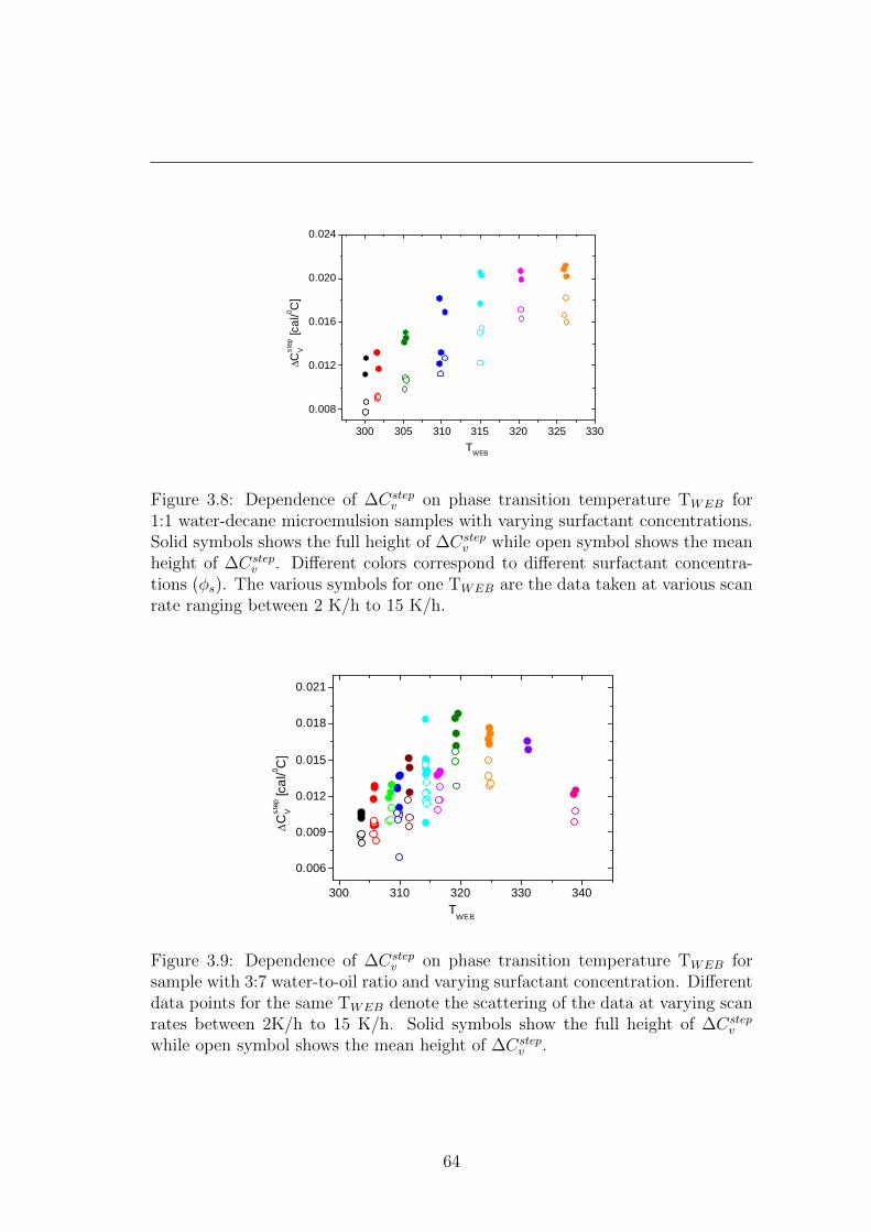
300 305 310 315 320 325 330

0.008

0.012

0.016

0.020

0.024

ΔC

step

V

[cal

/0 C]

TWEB

Figure 3.8: Dependence of ∆Cstepv on phase transition temperature TWEB for

1:1 water-decane microemulsion samples with varying surfactant concentrations.Solid symbols shows the full height of ∆Cstep

v while open symbol shows the meanheight of ∆Cstep

v . Different colors correspond to different surfactant concentra-tions (φs). The various symbols for one TWEB are the data taken at various scanrate ranging between 2 K/h to 15 K/h.

300 310 320 330 340

0.006

0.009

0.012

0.015

0.018

0.021

TWEB

ΔC

step

V

[cal

/0 C]

Figure 3.9: Dependence of ∆Cstepv on phase transition temperature TWEB for

sample with 3:7 water-to-oil ratio and varying surfactant concentration. Differentdata points for the same TWEB denote the scattering of the data at varying scanrates between 2K/h to 15 K/h. Solid symbols show the full height of ∆Cstep

v

while open symbol shows the mean height of ∆Cstepv .

64

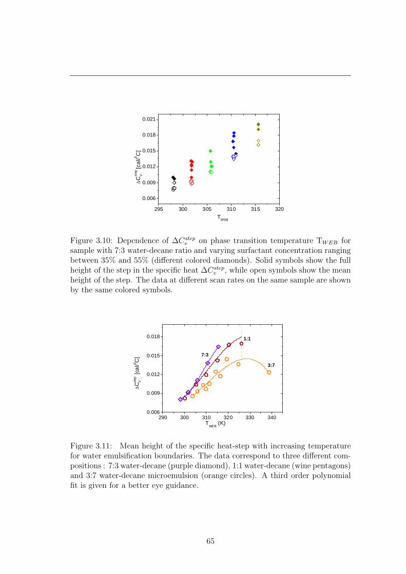
295 300 305 310 315 320

0.006

0.009

0.012

0.015

0.018

0.021

ΔC

step

V

[cal

/0 C]

TWEB

Figure 3.10: Dependence of ∆Cstepv on phase transition temperature TWEB for

sample with 7:3 water-decane ratio and varying surfactant concentration rangingbetween 35% and 55% (different colored diamonds). Solid symbols show the fullheight of the step in the specific heat ∆Cstep

v , while open symbols show the meanheight of the step. The data at different scan rates on the same sample are shownby the same colored symbols.

290 300 310 320 330 3400.006

0.009

0.012

0.015

0.018

ΔC

step

V

[cal

/0 C]

TWEB

(K)

7:3

1:1

3:7

Figure 3.11: Mean height of the specific heat-step with increasing temperaturefor water emulsification boundaries. The data correspond to three different com-positions : 7:3 water-decane (purple diamond), 1:1 water-decane (wine pentagons)and 3:7 water-decane microemulsion (orange circles). A third order polynomialfit is given for a better eye guidance.

65

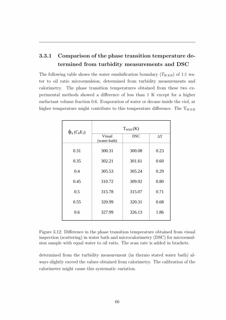
3.3.1 Comparison of the phase transition temperature de-

termined from turbidity measurements and DSC

The following table shows the water emulsification boundary (TWEB) of 1:1 wa-

ter to oil ratio microemulsion, determined from turbidity measurements and

calorimetry. The phase transition temperatures obtained from these two ex-

perimental methods showed a difference of less than 1 K except for a higher

surfactant volume fraction 0.6. Evaporation of water or decane inside the viol, at

higher temperature might contribute to this temperature difference. The TWEB

TWEB (K)

φs (C8E3)

Visual (water-bath)

DSC ΔT

0.31

0.35

0.4

0.45

0.5

0.55

0.6

300.31

302.21

305.53

310.72

315.78

320.99

327.99

300.08

301.61

305.24

309.92

315.07

320.31

326.13

0.23

0.60

0.29

0.80

0.71

0.68

1.86

Figure 3.12: Difference in the phase transition temperature obtained from visualinspection (scattering) in water bath and microcalorimetry (DSC) for microemul-sion sample with equal water to oil ratio. The scan rate is added in brackets.

determined from the turbidity measurement (in thermo stated water bath) al-

ways slightly exceed the values obtained from calorimetry. The calibration of the

calorimeter might cause this systematic variation.

66

3.4 Experiment Results of DLS

The average domain size of microemulsion samples is measured by dynamic light

scattering. Samples at 1Φ, 2Φ or 3Φ regions are chosen [FIG. 3.14]. Initially, the

refractive index of the microemulsion samples as a function of composition and

temperature is determined which enters the analysis of the DLS data later.

c) DLS

The dependence of the droplet size in a single phase region and two phase region is

studied. It is theoretically shown that the droplet size in a single phase region depends

only on the concentration of the components. But in a two phase region the size depends

only on temperature. Dynamic light scattering experiment underlines the above facts.

Change in the droplet size with temperature has been measured as shown in the table

below.

T (0C) 140C 170C 240C (1Φ) 320C 370C

14 % 7.5 8.26 5.75

22 % 3.43 5.08 7.6 6.36 4.14

27 % 3.31 5.1 6.97 6.48 5.61

φs calculated measured corrected

14% 10.28 8.264 (3φ) 8.31

22% 6.55 7.6 8.32

27% 5.35 6.97 7.269

Refractive index measurements:

Refractive index of the microemulsion in different macroscopic phases is required for the

light scattering data analysis. So the measurement of the sample at different temperature is

done with AB refractometer. All the values are obtained for a wavelength of (sodium

light).

T(0C) 110C 140C 240C 370C

14 % 1.377 1.394 1.406

22 % 1.389 1.397 1.406

27 % 1.397 1.397 1.406

40 % 1.405

φs

φs

Figure 3.13: Refractive index of the microemulsion samples with different surfac-tant concentrations at different temperatures.

The average domain size is measured for temperatures from 140C to 370C

[cross marks in FIG. 3.14]. The temperature dependence of the size of the

oil/water domains are shown in [FIG. 3.15]. The left most column lists φs for a

1:1 water-decane microemulsion.

The domain size in a two phase region depends on temperature and in the

one phase region on surfactant concnetration [Section X]. In the 1Φ region, the

average domain size for C8E3-water-decane microemulsion with φs = 27% is R1Φw

= 7.3 nm. After crossing TWEB, the droplets shrink by expelling excess water.

Hence, at 320C and 370C the domain size decreased to 6.5 nm and 5.6 nm re-

spectively. Below TOEB, the size of the oil domain decreased to 3.3 nm at 140C.

A similar trend can be seen for the other two sets of sample. Note, near to the

tricritcal point, the morphology of microemulsions is not spherical but bicontin-

uous. However, in data analysis a spherical morphology is assumed. Still, the

measured data reflect the typical length scale of the underlying morphology.

67

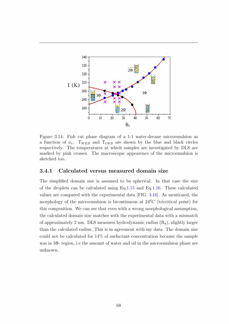
Φ2

Φ2

Φ1Φ3

Figure 3.14: Fish cut phase diagram of a 1:1 water-decane microemulsion asa function of φs. TWEB and TOEB are shown by the blue and black circlesrespectively. The temperatures at which samples are investigated by DLS aremarked by pink crosses. The macroscopic appearence of the microemulsion issketched too.

3.4.1 Calculated versus measured domain size

The simplified domain size is assumed to be spherical. In that case the size

of the droplets can be calculated using Eq.1.15 and Eq.1.16. These calculated

values are compared with the experimental data [FIG. 3.16]. As mentioned, the

morphology of the microemulsion is bicontinuous at 240C (tricritical point) for

this composition. We can see that even with a wrong morphological assumption,

the calculated domain size matches with the experimental data with a mismatch

of approximately 2 nm. DLS measures hydrodynamic radius (Rh), slightly larger

than the calculated radius. This is in agreement with my data. The domain size

could not be calculated for 14% of surfactant concentration because the sample

was in 3Φ- region, i.e the amount of water and oil in the microemulsion phase are

unknown.

68

5.66.57.35.13.327 %

4.16.48.35.13.422 %

5.88.37.514 %

370C(2Φ)

320C(2Φ)

240C (1Φ/3Φ)

170C(2Φ)

140C(2Φ)

T (0C)φs

7.35.427%

8.36.622%

8.3 (3φ)10.314%

measured domain size

(nm)

calculated R (nm)

φs

R (nm)

Figure 3.15: Hydrodynamic radius of oil/water domains obtained from DLS.Microemulsion samples with 1:1 water-decane and three different surfactant con-centrations are used.

5.66.57.35.13.327 %

4.16.48.35.13.422 %

5.88.37.514 %

370C(2Φ)

320C(2Φ)

240C (1Φ/3Φ)

170C(2Φ)

140C(2Φ)

T (0C)φs

7.35.427%

8.36.622%

8.3 (3φ)14%

measured domain size

(nm)

calculated R (nm)

φs

R (nm)

Figure 3.16: Calculated and the experimental data (DLS) of the domain sizes of1:1 water-decane microemulsion sample with varying surfactant concentration at240C. Results are presented in nanometers.

69

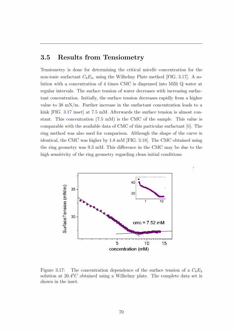
3.5 Results from Tensiometry

Tensiometry is done for determining the critical micelle concentration for the

non-ionic surfactant C8E3, using the Wilhelmy Plate method [FIG. 3.17]. A so-

lution with a concentration of 4 times CMC is dispensed into Milli Q water at

regular intervals. The surface tension of water decreases with increasing surfac-

tant concentration. Initially, the surface tension decreases rapidly from a higher

value to 38 mN/m. Further increase in the surfactant concentration leads to a

kink [FIG. 3.17 inset] at 7.5 mM. Afterwards the surface tension is almost con-

stant. This concentration (7.5 mM) is the CMC of the sample. This value is

comparable with the available data of CMC of this particular surfactant [6]. The

ring method was also used for comparison. Although the shape of the curve is

identical, the CMC was higher by 1.8 mM [FIG. 3.18]. The CMC obtained using

the ring geometry was 9.3 mM. This difference in the CMC may be due to the

high sensitivity of the ring geometry regarding clean initial conditions.

Figure 3.17: The concentration dependence of the surface tension of a C8E3

solution at 20.40C obtained using a Wilhelmy plate. The complete data set isshown in the inset.

70

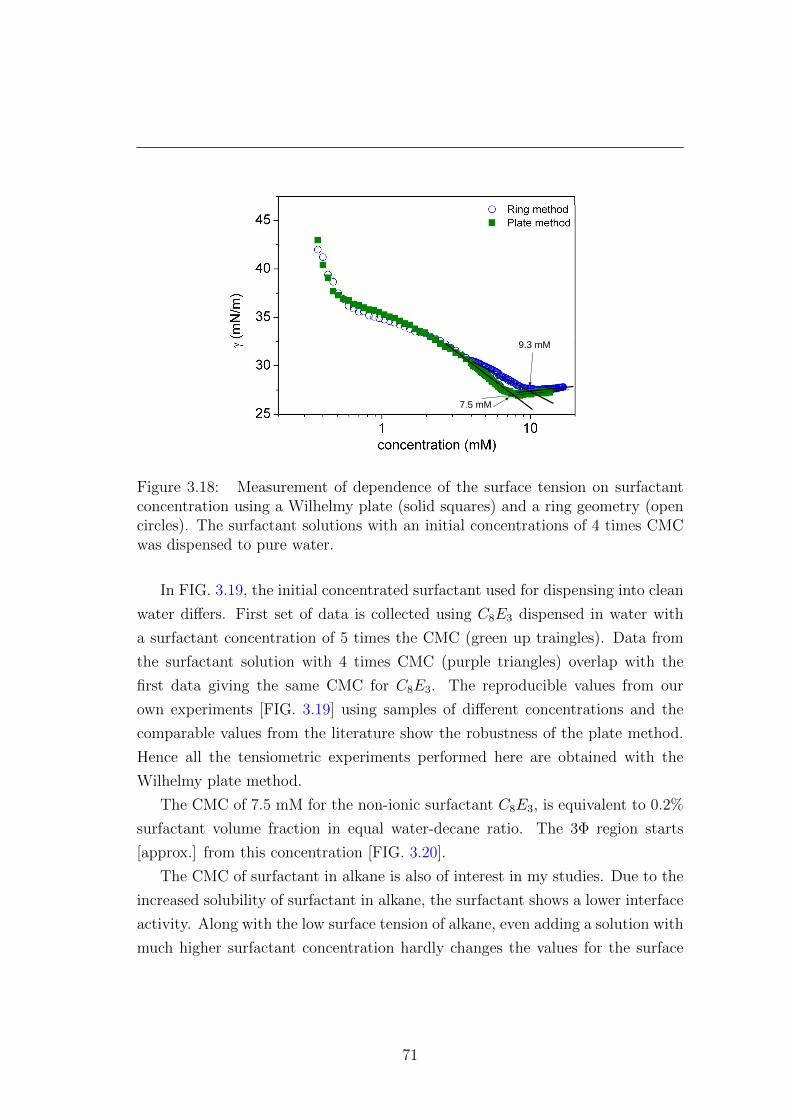
7.5 mM

9.3 mM

Figure 3.18: Measurement of dependence of the surface tension on surfactantconcentration using a Wilhelmy plate (solid squares) and a ring geometry (opencircles). The surfactant solutions with an initial concentrations of 4 times CMCwas dispensed to pure water.

In FIG. 3.19, the initial concentrated surfactant used for dispensing into clean

water differs. First set of data is collected using C8E3 dispensed in water with

a surfactant concentration of 5 times the CMC (green up traingles). Data from

the surfactant solution with 4 times CMC (purple triangles) overlap with the

first data giving the same CMC for C8E3. The reproducible values from our

own experiments [FIG. 3.19] using samples of different concentrations and the

comparable values from the literature show the robustness of the plate method.

Hence all the tensiometric experiments performed here are obtained with the

Wilhelmy plate method.

The CMC of 7.5 mM for the non-ionic surfactant C8E3, is equivalent to 0.2%

surfactant volume fraction in equal water-decane ratio. The 3Φ region starts

[approx.] from this concentration [FIG. 3.20].

The CMC of surfactant in alkane is also of interest in my studies. Due to the

increased solubility of surfactant in alkane, the surfactant shows a lower interface

activity. Along with the low surface tension of alkane, even adding a solution with

much higher surfactant concentration hardly changes the values for the surface

71

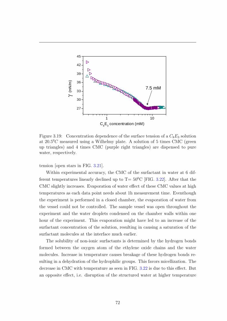
1 10

27

30

33

36

39

42

45

WPlate 5CMC WPlate 4CMC

file: Graph: Graph1 Date: 12/12/2011 09:01

γ (m

N/m

)

C8E3 concentration (mM)

7.5 mM

Figure 3.19: Concentration dependence of the surface tension of a C8E3 solutionat 20.50C measured using a Wilhelmy plate. A solution of 5 times CMC (greenup triangles) and 4 times CMC (purple right triangles) are dispensed to purewater, respectively.

tension [open stars in FIG. 3.21].

Within experimental accuracy, the CMC of the surfactant in water at 6 dif-

ferent temperatures linearly declined up to T= 500C [FIG. 3.22]. After that the

CMC slightly increases. Evaporation of water effect of these CMC values at high

temperatures as each data point needs about 1h measurement time. Eventhough

the experiment is performed in a closed chamber, the evaporation of water from

the vessel could not be controlled. The sample vessel was open throughout the

experiment and the water droplets condensed on the chamber walls within one

hour of the experiment. This evaporation might have led to an increase of the

surfactant concentration of the solution, resulting in causing a saturation of the

surfactant molecules at the interface much earlier.

The solubility of non-ionic surfactants is determined by the hydrogen bonds

formed between the oxygen atom of the ethylene oxide chains and the water

molecules. Increase in temperature causes breakage of these hydrogen bonds re-

sulting in a dehydration of the hydrophilic groups. This favors micellization. The

decrease in CMC with temperature as seen in FIG. 3.22 is due to this effect. But

an opposite effect, i.e. disruption of the structured water at higher temperature

72

0 10 20 30 40 50 60 70

280

300

320

340

T

φs

50:50

φs ∼ 0.2%

Figure 3.20: Appearance of 3Φ region(red dotted line) according to the CMC ofC8E3 in water. The experimental data for the emulsification boundaries[TWEB

[green squares] and TOEB [blue squares]] for 1:1 water to oil ratio microemulsionwith varying surfactant concentration.

can disfavor micellization [11]. A minimum in the CMC-temperature curve is due

to domination of this effect over micellization. Experiments on strong surfactant

C12E5 showed a similar trend as in [FIG. 3.22] [10].

73

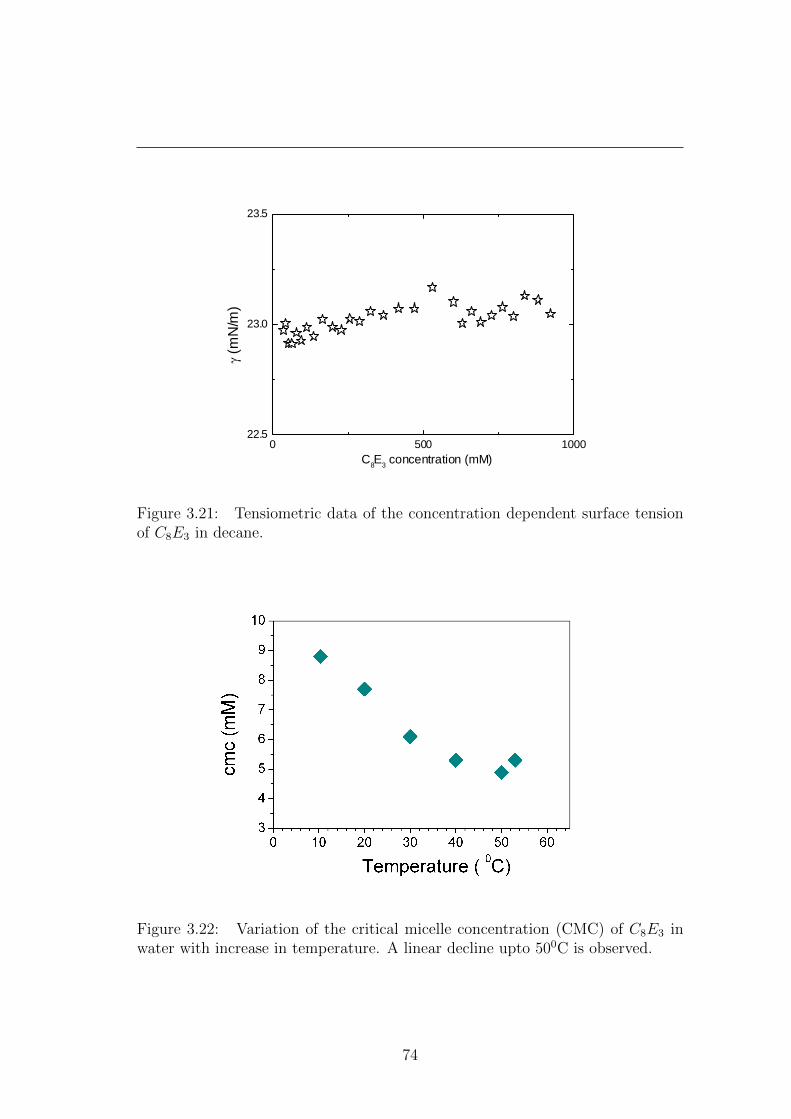
0 500 100022.5

23.0

23.5

γ (m

N/m

)

C8E3 concentration (mM)

Figure 3.21: Tensiometric data of the concentration dependent surface tensionof C8E3 in decane.

Figure 3.22: Variation of the critical micelle concentration (CMC) of C8E3 inwater with increase in temperature. A linear decline upto 500C is observed.

74

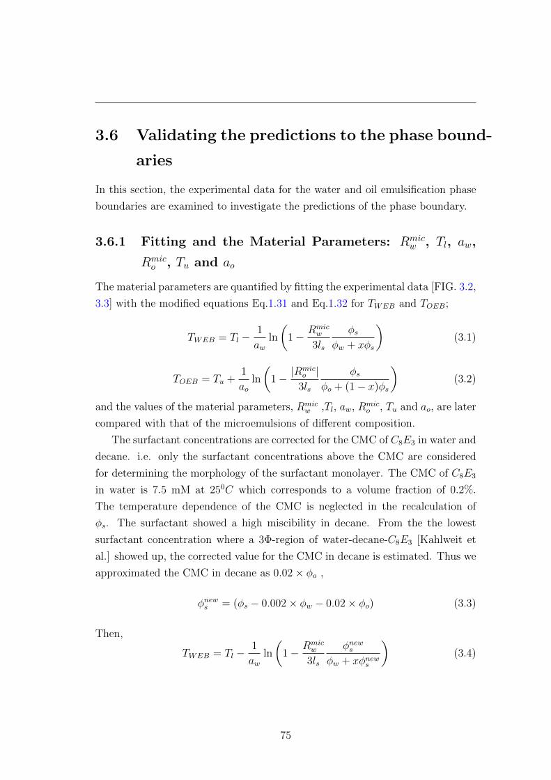
3.6 Validating the predictions to the phase bound-

aries

In this section, the experimental data for the water and oil emulsification phase

boundaries are examined to investigate the predictions of the phase boundary.

3.6.1 Fitting and the Material Parameters: Rmicw , Tl, aw,

Rmico , Tu and ao

The material parameters are quantified by fitting the experimental data [FIG. 3.2,

3.3] with the modified equations Eq.1.31 and Eq.1.32 for TWEB and TOEB;

TWEB = Tl −1

awln

(1− Rmic

w

3ls

φsφw + xφs

)(3.1)

TOEB = Tu +1

aoln

(1− |R

mico |

3ls

φsφo + (1− x)φs

)(3.2)

and the values of the material parameters, Rmicw ,Tl, aw, Rmic

o , Tu and ao, are later

compared with that of the microemulsions of different composition.

The surfactant concentrations are corrected for the CMC of C8E3 in water and

decane. i.e. only the surfactant concentrations above the CMC are considered

for determining the morphology of the surfactant monolayer. The CMC of C8E3

in water is 7.5 mM at 250C which corresponds to a volume fraction of 0.2%.

The temperature dependence of the CMC is neglected in the recalculation of

φs. The surfactant showed a high miscibility in decane. From the the lowest

surfactant concentration where a 3Φ-region of water-decane-C8E3 [Kahlweit et

al.] showed up, the corrected value for the CMC in decane is estimated. Thus we

approximated the CMC in decane as 0.02× φo ,

φnews = (φs − 0.002× φw − 0.02× φo) (3.3)

Then,

TWEB = Tl −1

awln

(1− Rmic

w

3ls

φnews

φw + xφnews

)(3.4)

75

TWEB = Tu +1

aoln

(1− Rmic

o

3ls

φnews

φw + (1− x)φnews

)(3.5)

3.6.2 Interfacial surfactant after the CMC correction

Including the CMC of the surfactant in water and decane in Eq.3.4 we estimated

the interfacial active surfactant. This corrected value for the surfactant volume

fraction has been used in further studies. Despite the high solubility of C8E3 in

decane, the interfacial active surfactant is only just below the total surfactant

concentration. This is due to the high surfactant concentration, i.e. low volume

fraction of decane.

0.630.640.510.520.410.420.310.320.230.240.190.210.120.13

newsφsφ (total surf.) (interfacial)

Figure 3.23: Table showing the actual volume fraction of the surfactant in thesample and the interfacial active surfactant obtained using the equation 3.3

for equal volume fraction of water and decane.

3.6.3 Microemulsion with equal proportion of water and

decane (1:1)

The experimental data for TWEB and TOEB for C8E3-water-decane microemul-

sion with equal proportions of water and decane is shown in FIG. 3.24. TWEB

of the sample investigated between φs = 0.15 to 0.65 increases with increasing

76

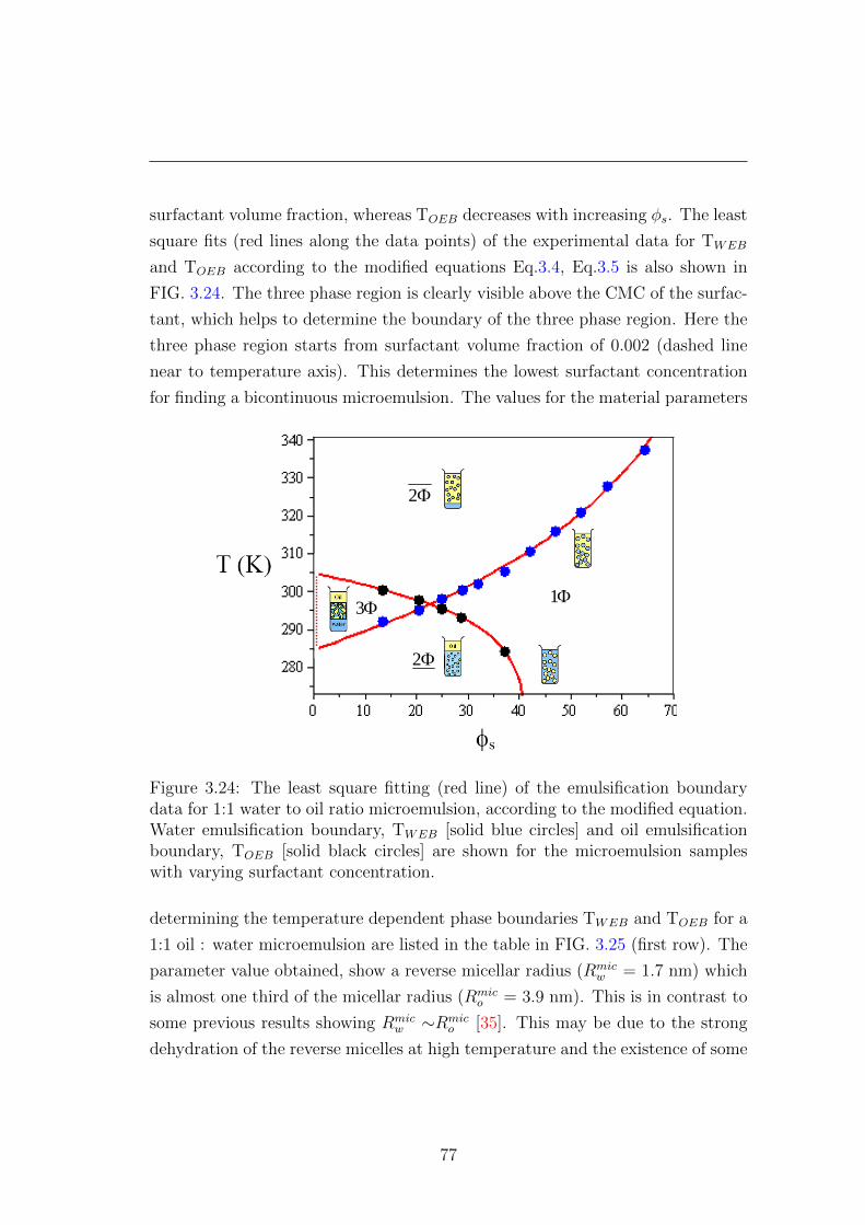
surfactant volume fraction, whereas TOEB decreases with increasing φs. The least

square fits (red lines along the data points) of the experimental data for TWEB

and TOEB according to the modified equations Eq.3.4, Eq.3.5 is also shown in

FIG. 3.24. The three phase region is clearly visible above the CMC of the surfac-

tant, which helps to determine the boundary of the three phase region. Here the

three phase region starts from surfactant volume fraction of 0.002 (dashed line

near to temperature axis). This determines the lowest surfactant concentration

for finding a bicontinuous microemulsion. The values for the material parameters

Φ2

Φ2

Φ1Φ3

Figure 3.24: The least square fitting (red line) of the emulsification boundarydata for 1:1 water to oil ratio microemulsion, according to the modified equation.Water emulsification boundary, TWEB [solid blue circles] and oil emulsificationboundary, TOEB [solid black circles] are shown for the microemulsion sampleswith varying surfactant concentration.

determining the temperature dependent phase boundaries TWEB and TOEB for a

1:1 oil : water microemulsion are listed in the table in FIG. 3.25 (first row). The

parameter value obtained, show a reverse micellar radius (Rmicw = 1.7 nm) which

is almost one third of the micellar radius (Rmico = 3.9 nm). This is in contrast to

some previous results showing Rmicw ∼Rmic

o [35]. This may be due to the strong

dehydration of the reverse micelles at high temperature and the existence of some

77

oil in the micelles due to the high solubility of the surfactant in oil. The change

of a swollen micelle to a micelle or reverse micelle is quantified using the material

parameter ao and aw. The meaning of ao and aw will be discussed in detail in

later sections.

ao(K-1)

Tu (K)

Ro (nm)

aw(K-1)

Tl (K)

Rw (nm)

water : decane

0.103043.40.0262851.71 : 1

0.07

0.15

306

304

3.0

5.1

0.0282841.97 : 3

0.0292861.83 : 7

mic mic

Figure 3.25: Values for the parameters from the fitting of the emulsificationboundary data for 1:1, 3:7 and 7:3 water to oil ratio microemulsion accordingto the modified Helfrich equation. Fitting of TWEB yielded Rmic

w , Tl and aw.The effective length of the surfactant is kept fixed, ls = 1nm. Fitting of the oilemulsification boundary, TOEB gave Rmic

o , Tu and ao.

3.6.4 Microemulsion with 3:7 and 7:3 water to decane ra-

tio

The trend of the phase boundaries with increasing temperature for 3:7 and 7:3

water to decane microemulsions are the same as in the previous sample. A change

in the water to decane ratio changed the location of the tricritical point (T ). For

the 3:7 composition, we can see that for φs > 36%, all the oil is emulsified for

temperature above the freezing point of water. Whereas, at higher temperatures

water still gets expelled out. For the 7:3 composition, at φs > 32% all the oil is

emulsified while water still expelles out at higher temperatures. The experimental

data for TWEB and TOEB of 3:7 and 7:3 water- oil microemulsions are fitted using

the modified equations Eq.3.4, Eq.3.5. The values of the material parameters

obtained from the fit are given in the last two rows of FIG. 3.25.

From the table [FIG. 3.25] we can see that the values of the material param-

78

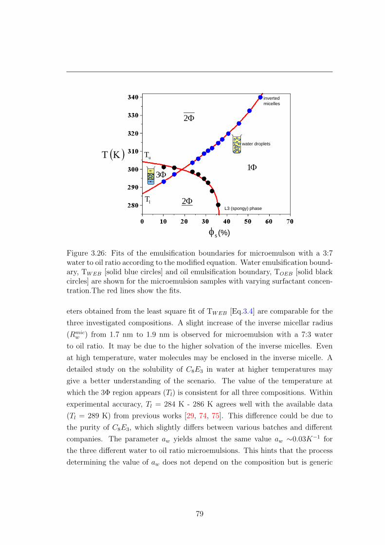
sφ (%)

lT

uT

L3 (spongy) phase

inverted micelles

Φ2

Φ2

Φ1Φ3

water droplets

( )ΚT

Figure 3.26: Fits of the emulsification boundaries for microemulson with a 3:7water to oil ratio according to the modified equation. Water emulsification bound-ary, TWEB [solid blue circles] and oil emulsification boundary, TOEB [solid blackcircles] are shown for the microemulsion samples with varying surfactant concen-tration.The red lines show the fits.

eters obtained from the least square fit of TWEB [Eq.3.4] are comparable for the

three investigated compositions. A slight increase of the inverse micellar radius

(Rmicw ) from 1.7 nm to 1.9 nm is observed for microemulsion with a 7:3 water

to oil ratio. It may be due to the higher solvation of the inverse micelles. Even

at high temperature, water molecules may be enclosed in the inverse micelle. A

detailed study on the solubility of C8E3 in water at higher temperatures may

give a better understanding of the scenario. The value of the temperature at

which the 3Φ region appears (Tl) is consistent for all three compositions. Within

experimental accuracy, Tl = 284 K - 286 K agrees well with the available data

(Tl = 289 K) from previous works [29, 74, 75]. This difference could be due to

the purity of C8E3, which slightly differs between various batches and different

companies. The parameter aw yields almost the same value aw ∼0.03K−1 for

the three different water to oil ratio microemulsions. This hints that the process

determining the value of aw does not depend on the composition but is generic

79

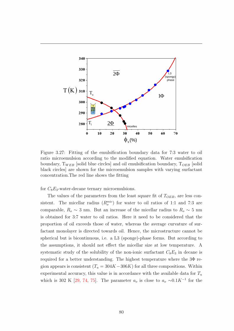
sφ (%)

( )ΚT

lT

uT

L3 (spongy)

phase

micellesΦ2

Φ2

Φ1

Figure 3.27: Fitting of the emulsification boundary data for 7:3 water to oilratio microemulsion according to the modified equation. Water emulsificationboundary, TWEB [solid blue circles] and oil emulsification boundary, TOEB [solidblack circles] are shown for the microemulsion samples with varying surfactantconcentration.The red line shows the fitting

for C8E3-water-decane ternary microemulsions.

The values of the parameters from the least square fit of TOEB, are less con-

sistent. The micellar radius (Rmico ) for water to oil ratios of 1:1 and 7:3 are

comparable, Ro ∼ 3 nm. But an increase of the micellar radius to Ro ∼ 5 nm

is obtained for 3:7 water to oil ratios. Here it need to be considered that the

proportion of oil exceeds those of water, whereas the average curvature of sur-

factant monolayer is directed towards oil. Hence, the microstructure cannot be

spherical but is bicontinuous, i.e. a L3 (sponge)-phase forms. But according to

the assumptions, it should not effect the micellar size at low temperature. A

systematic study of the solubility of the non-ionic surfactant C8E3 in decane is

required for a better understanding. The highest temperature where the 3Φ re-

gion appears is consistent (Tu = 304K−306K) for all three compositions. Within

experimental accuracy, this value is in accordance with the available data for Tu

which is 302 K [29, 74, 75]. The parameter ao is close to ao ∼0.1K−1 for the

80

three investigated ratios of water to oil. Again, ao is slightly higher for water

to oil ratios of 3:7. Similar to aw, the consistency in the value of ao, points

towards a generic process that does not depend on the ratio of water to oil in

microemulsions.

As already mentioned, the morphology of the microemulsion at the emulsi-

fication boundaries depends on composition. The underlying morphology can

be bicontinuous, sponge-like, cylindrical and spherical. Close to tricritical point

T , the distribution of water and oil will be similar on either side of the sur-

factant monolayer in a bicontinuous morphology. However, in the derivation of

the modified equation it is assumed that the surfactant monolayer is spherical.

Amazingly, even with the wrong assumption of a droplet morphology, the phase

boundaries near to the tricritical point are fitted very well. The consistency in

the parameter values for different proportions of water to oil, keeping all other

conditions constant, points that the factor determining the phase boundaries or

the emulsification failure depends only on the choice of the surfactant and oil.

3.7 Prediction of the phase boundaries

Next, the predictive power of the expressions for TWEB and TOEB is evaluated.

Henceforth, we insert the material parameter values of the 1:1 water to oil ratio to

calculate the phase boundaries according to Eq.3.4 and Eq.3.5. An equal propor-

tion of water and oil gave a symmetric fish cut horizontally along the tricritical

point. This calculated parameter free expression for the phase boundaries is then

compared with the experimental data for TWEB and TOEB.

The predicted phase transitions (green lines) for the water and oil emulsifica-

tion boundaries [TWEB and TOEB] is plotted with the experimental data points of

3:7 water to decane in FIG. 3.28. Here the parameter free prediction for the TWEB

matches very well with the experimental data. In case of TOEB, the phase bound-

ary determined from experiment is well described for low values of φs. However,

when increasing the surfactant concentration the experimental data points stay

below the theoretical prediction. A possible explanation for this deviation can be

that microemulsion has an L3 (sponge-like) morphology at lower temperature and

is not spherical as assumed in the equation. An L3- morphology implies that the

81

T (K)Φ1

lT

uT

L3 (sponge)phase

inverted micelles

water droplets

Φ2

Φ3

sφ (%)

Figure 3.28: Experimental data for the water emulsification boundary, TWEB

[solid blue circles] and oil emulsification boundary TOEB [solid black circles] of3:7 water to oil ratio microemulsion. Predicted emulsification boundaries withthe modified equations is given as green lines.

surfactant molecules self assemble in the form of bilayers instead of monolayers.

Still, within the achievable experimental parameters, the prediction describes the

experimental observations quite well. In FIG. 3.29, the experimental data for

TWEB and TOEB of 7:3 water to decane is plotted along with the predicted phase

boundaries (green lines). An amazingly well matching between the predicted

TWEB and the experimental data is observed, although the underlying morphol-

ogy is L3 (sponge-like). Surprisingly, the bilayer morphology has little influence

on the phase behaviour in the curvature towards water. The TOEB prediction

also matches well with the experimental data within the experimental accuracy.

Again, an increased discrepancy is observed at higher surfactant concentration.

However, in this case the experimentally observed phase boundary exceeds the

predicted boundary by about 20C.

Inorder to test the validity of the predictions, a different section of the phase

prism is chosen too [FIG. 3.30]. Here the surfactant concentration is kept constant

82

T (K)

Φ1

L3 (sponge)

phase

oil drops

Φ2

sφ (%)

Figure 3.29: Plotting of the emulsification boundary for 7:3 water to oil ratiomicroemulsion according to the prediction with the modified equation (greenline). Experimental data for the water emulsification boundary, TWEB [solidblue circles] are shown for the microemulsion samples with varying surfactantconcentration.

and the parameter αo, i.e. the ratio of oil to water plus oil (αo = φo/(φw + φo))

is varied. At low temperature (T < Tl) and high water proportion, surfactants

are well hydrated with the water molecules. Hence the surfactant monolayer

bend towards oil. An increase in temperature leads to the dehydration of the

surfactant molecules, changing the curvature of the monolayer and hence the

microstructure of the microemulsion. For (Tl < T < Tu), the surfactant possess a

bicontinuous structure, with surfactant monolayer bending towards both oil and

water molecules. Dehydration of the surfactant molecules at higher temperatures

(T > Tu), bends the surfactant monolayer to enclose water molecules.

Three different sets of experimental data for TWEB and TOEB are shown which

correspond to three different surfactant concentration - 35% (green circles), 40%

(blue circles) and 50% (orange circles) respectively. The parameter-free predic-

tions are calculated using the material parameters given in FIG. 3.25 for 1:1 water

83

0.0 0.2 0.4 0.6 0.8 1.0

280

300

320

340

T (K

)

αo

2Φ

2Φ

1Φ

Tu

Tl

TWEB

TOEB

bicontinuous(sponge-like)

bicontinuous(sponge-like)

Figure 3.30: Experimental data for the evolution of water and oil emulsificationboundaries with temperature and varying αo are given by solid and open circlesrespectively. Surfactant concentration is fixed at 35% (green), 40% (blue) and50% (orange). The predictions (lines) for the water emulsification boundaries(solid lines) and the oil emulsification boundaries (dotted lines) according to themodified equation for the three different surfactant concentrations are shown.The dashed line shows the temperature Tl and Tu. Microstructure of the sampleat various temperatures are sketched.

84

to oil ratio. So there are no free-parameters in the modified equation used for

the prediction-plots. The experimental data and the calculated phase boundaries

are shown in FIG. 3.30. They match quite well except at higher values of αo,

where a slight mismatch is observed. In the 1φ-channel, between Tu (304 K) and

Tl (285 K), the microstructure of the emulsion is bicontinuous. For αo ≤ 0.6, the

surfactant monolayer is bicontinuous for samples with comparatively low surfac-

tant concentrations, φs = 35% and 40%, while for φs = 50%, the morphology is

spherical. Again for φs = 50%, morphology takes a bicontinuous structure for

αo ≤ 0.15.

Eventhough all the assumptions are made for a spherical morphology, the

modified Helfrich equation predicts the regions with bicontinuous structure (data

at intermediate temperature) amazingly well. This leads to an assumption that

the bicontinuous structure may be equivalent to broken pieces of spherical droplets,

where some pieces have a preferred curvature towards oil and the other towards

water. At higher values of αo (above 0.6) a deviation (5 K-10 K) of the predic-

tion from the experimental data is observed for the water emulsification boundary.

Considering a low value for the experimental data than expected TWEB, at higher

αo, is due to the cylindrical and ellipsoidal shape formed by the water domains

due to conservation of total interfacial area and internal water volume [76]. The

oil emulsification boundaries (TOEB) shift away from the water emulsification

boundaries with increase in the surfactant concentration, making the 1φ-channel

wider. Higher surfactant concentration in the microemulsion sample stabilises

the water and oil domains, preventing phase separation. Within the bicontinuous

regime, the experimentally determined oil emulsification boundaries for φs = 35%

and 40%, agrees well with the predicted phase boundaries, whereas, the exper-

imentally determined values for TOEB at αo > 0.6 and φs = 40% showed lower

phase boundaries than the predicted phase boundaries.

85

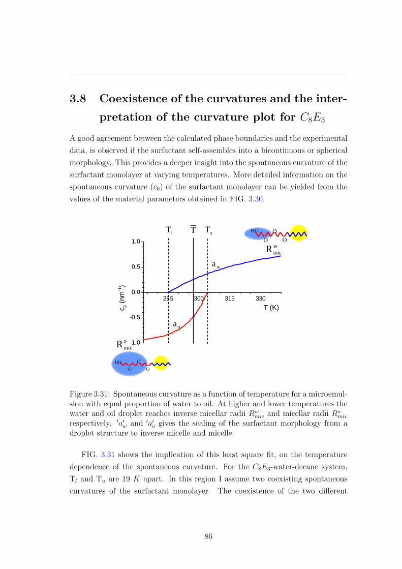
3.8 Coexistence of the curvatures and the inter-

pretation of the curvature plot for C8E3

A good agreement between the calculated phase boundaries and the experimental

data, is observed if the surfactant self-assembles into a bicontinuous or spherical

morphology. This provides a deeper insight into the spontaneous curvature of the

surfactant monolayer at varying temperatures. More detailed information on the

spontaneous curvature (c0) of the surfactant monolayer can be yielded from the

values of the material parameters obtained in FIG. 3.30.

285 300 315 330

-1.0

-0.5

0.0

0.5

1.0

c 0 (nm

-1)

T (K)

OHO O

O

OHO O

O

wmicR

wa

oa

omicR

lT uTT

Figure 3.31: Spontaneous curvature as a function of temperature for a microemul-sion with equal proportion of water to oil. At higher and lower temperatures thewater and oil droplet reaches inverse micellar radii Rw

mic and micellar radii Romic

respectively. ′a′w and ′a′o gives the scaling of the surfactant morphology from adroplet structure to inverse micelle and micelle.

FIG. 3.31 shows the implication of this least square fit, on the temperature

dependence of the spontaneous curvature. For the C8E3-water-decane system,

Tl and Tu are 19 K apart. In this region I assume two coexisting spontaneous

curvatures of the surfactant monolayer. The coexistence of the two different

86

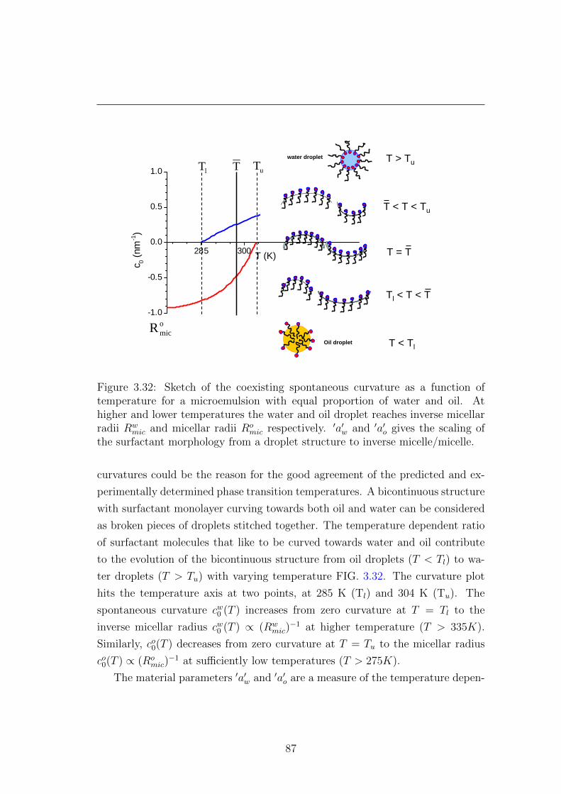
T (K)285 300

-1.0

-0.5

0.0

0.5

1.0

c 0 (nm

-1)

T > Tu

T < T < Tu

T = T

Tl < T < T

T < TlOil droplet

water droplet

lT T uT

omicR

Figure 3.32: Sketch of the coexisting spontaneous curvature as a function oftemperature for a microemulsion with equal proportion of water and oil. Athigher and lower temperatures the water and oil droplet reaches inverse micellarradii Rw

mic and micellar radii Romic respectively. ′a′w and ′a′o gives the scaling of

the surfactant morphology from a droplet structure to inverse micelle/micelle.

curvatures could be the reason for the good agreement of the predicted and ex-

perimentally determined phase transition temperatures. A bicontinuous structure

with surfactant monolayer curving towards both oil and water can be considered

as broken pieces of droplets stitched together. The temperature dependent ratio

of surfactant molecules that like to be curved towards water and oil contribute

to the evolution of the bicontinuous structure from oil droplets (T < Tl) to wa-

ter droplets (T > Tu) with varying temperature FIG. 3.32. The curvature plot

hits the temperature axis at two points, at 285 K (Tl) and 304 K (Tu). The

spontaneous curvature cw0 (T ) increases from zero curvature at T = Tl to the

inverse micellar radius cw0 (T ) ∝ (Rwmic)

−1 at higher temperature (T > 335K).

Similarly, co0(T ) decreases from zero curvature at T = Tu to the micellar radius

co0(T ) ∝ (Romic)

−1 at sufficiently low temperatures (T > 275K).

The material parameters ′a′w and ′a′o are a measure of the temperature depen-

87

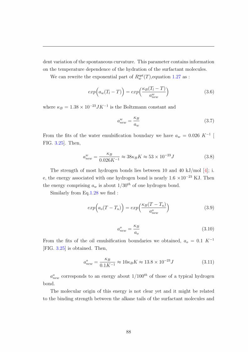
dent variation of the spontaneous curvature. This parameter contains information

on the temperature dependence of the hydration of the surfactant molecules.

We can rewrite the exponential part of Roptw (T ),equation 1.27 as :

exp(aw(Tl − T )

)= exp

(κB(Tl − T )

awnew

)(3.6)

where κB = 1.38× 10−23JK−1 is the Boltzmann constant and

awnew =κBaw

(3.7)

From the fits of the water emulsification boundary we have aw = 0.026 K−1 [

FIG. 3.25]. Then,

awnew =κB

0.026K−1≈ 38κBK ≈ 53× 10−23J (3.8)

The strength of most hydrogen bonds lies between 10 and 40 kJ/mol [4]; i.

e, the energy associated with one hydrogen bond is nearly 1.6 ×10−23 KJ. Then

the energy comprising aw is about 1/30th of one hydrogen bond.

Similarly from Eq.1.28 we find :

exp(ao(T − Tu)

)= exp

(κB(T − Tu)aonew

)(3.9)

aonew =κBao

(3.10)

From the fits of the oil emulsification boundaries we obtained, ao = 0.1 K−1

[FIG. 3.25] is obtained. Then,

aonew =κB

0.1K−1≈ 10κBK ≈ 13.8× 10−23J (3.11)

aonew corresponds to an energy about 1/100th of those of a typical hydrogen

bond.

The molecular origin of this energy is not clear yet and it might be related

to the binding strength between the alkane tails of the surfactant molecules and

88

decane or to the interactions between the hydrophilic head with water molecules.

89

3.9 Prediction of the step of the specific heat

The specific heat is an extremely sensitive probe of the temperature dependence

of the free energies, since it involves the second derivative of the temperature.

Hence it probes the curvature of the free energy. From the material parameters

obtained from the least square fits of the phase boundary data, we predict the

values of the step of the specific heat. The curvature value is then inserted into

Eq.1.42 to yield the height of the step in the specific heat. The height of the

specific heat-step depends on the square of the first derivative of the spontaneous

curvature with respect to temperature as,

∆Cstepv =

4κφsT

ls.

1

1 + κ2κ

(∂c0

∂T

)2

(3.12)295 300 305 310 315 320 325

0.00

0.04

0.08

0.12

0.16φs = 0.55

φs = 0.45

Cst

ep

v(J

K-1

cm

-3)

T (K)

φs = 0.31

295 300 305 310 315 320 325

0.00

0.04

0.08

0.12

0.16

0.20

φs = 0.55

φs = 0.45

ΔCst

ep

v(J

K-1 c

m-3)

T (K)

φs = 0.31

Figure 3.33: Temperature dependent variation of the specific heat for equal waterto oil ratio and surfactant concentration φs = 0.31 (orange diamonds), φs =0.45 (purple diamonds) and φs = 0.55 (dark cyan diamonds). Data has beensubtracted with a baseline. Mean height of the specific heat and the prediction(with the pre-factor) are shown. The thermograms are taken at 5 K/h acrosswater emulsification boundary.

Prediction of ∆Cstepv according to Eq.3.12 yield values well below the exper-

imentally determined height of ∆Cstepv . This lead to redefining the temperature

90

’T’ in Eq.3.12. In water-oil-nonionic microemulsion, as the macroscopic phase

transition temperatures of the microemulsion system starts from the upper (Tu)

and the lower(Tl) phase boundaries of a 3φ-region, a temperature pre-factor is

added to Eq.3.12. This prefactor,(T − Tl)/(Tu − Tl), should account for the ma-

terial curved towards water or oil. Addition of this concept (Eq.3.13) predicted

the height of the extremely sensitive specific heat-step well.

∆Cstepv =

4κφsT (T − Tl)ls(Tu − Tl)

.1

1 + κ2κ

(∂c0

∂T

)2

(3.13)

The variation of the specific heat with temperature for microemulsion samples

are given in FIG. 3.33 when crossing the water emulsification boundary 1φ - 2φ.

The consistency of the mean height of the specific heat-step from the calorimetry

(dashed line) and the theoretical prediction according to the above equation (grey

solid line) is checked for three different samples with equal water to oil ratio and

increasing surfactant concentration φs = 0.31 (orange diamonds) to φs = 0.55

(dark cyan diamonds) are shown. The specific heat-height increases with increase

in the surfactant concentration.

FIG. 3.34 shows the mean height in the specific heat step when crossing TWEB

for microemulsions with three different water to oil ratio and varying surfac-

tant concentrations. Accordingly the phase transition temperatures range over a

wide region from 295 K to 340 K. Open circles shows the data obtained through

calorimetry experiments. The predictons according to the Eq.3.12 and Eq.3.13

are given by green dashed and solid grey lines respectively. Eq.3.13 used the

parameter values obtained from the least square fit of phase diagram: Tu = 304

K and Tl = 285 K.

The data from the experiments and the predictions showed non-linearity in

the height of the specific heat step with increase in temperature. The non-linear

curve showed a saturation at T ∼ 320K for 1:1 and 3:7 water to decane ratio. The

non-linearity is related to the curvature of the surfactant monolayer. Along the

temperature range investigated, the surfactant monolayer encloses water. With

increasing temperature, the curvature of the surfactant monolayer also increases

leading the water domains enclosed by surfactant monolayer approaching inverse

micellar radius. From the phase behavior studies, no significant change is ob-

91

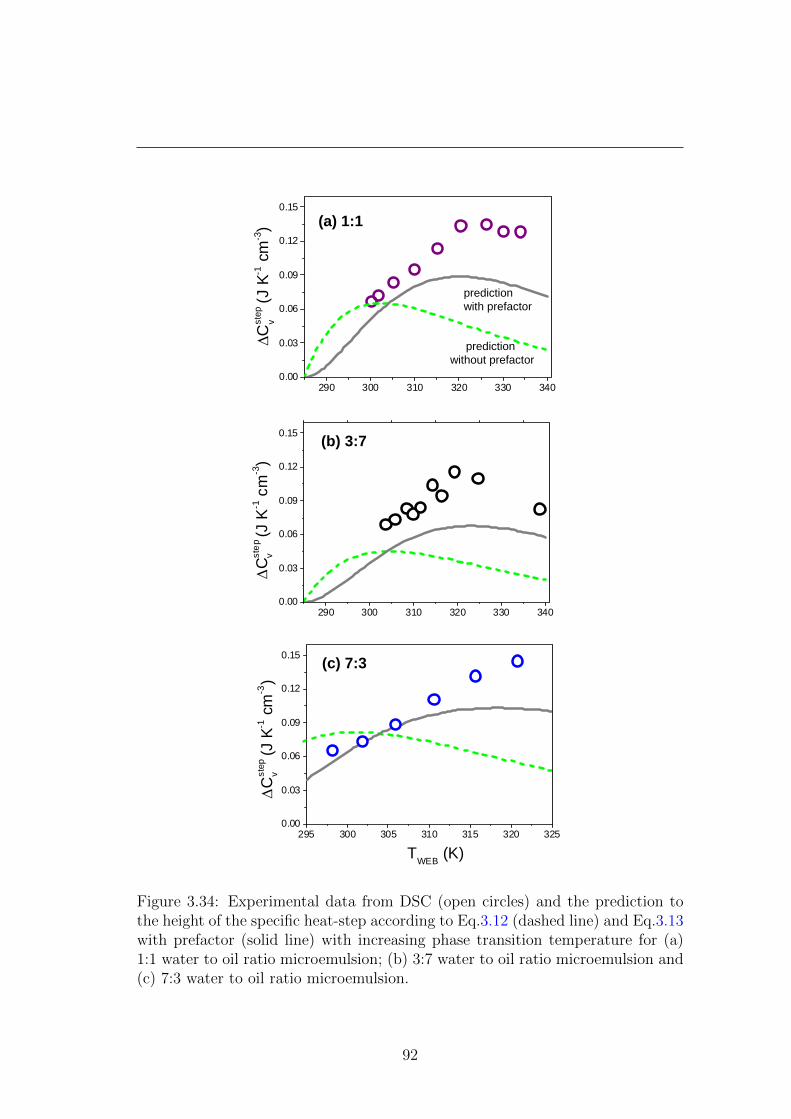
300 310 320 330

0.06

0.09

0.12

0.15

ΔC

step

v

(J K

-1 c

m-3

)

300 310 320 330 340

0.06

0.09

0.12

0.15

ΔC

step

v

(J K

-1 c

m-3)

295 300 305 310 315 320 325

0.06

0.09

0.12

0.15

TWEB (K)

ΔC

step

v

(J K

-1 c

m-3

)

(a) 1:1

(b) 3:7

(c) 7:3

290 300 310 320 330 3400.00

0.03

0.06

0.09

0.12

0.15

ΔCst

ep

v(J

K-1 c

m-3)

290 300 310 320 330 3400.00

0.03

0.06

0.09

0.12

0.15

ΔC

step

v

(J K

-1 c

m-3)

295 300 305 310 315 320 3250.00

0.03

0.06

0.09

0.12

0.15

TWEB (K)

ΔC

step

v

(J K

-1 c

m-3

)

(a) 1:1

(b) 3:7

(c) 7:3

prediction with prefactor

prediction without prefactor

Figure 3.34: Experimental data from DSC (open circles) and the prediction tothe height of the specific heat-step according to Eq.3.12 (dashed line) and Eq.3.13with prefactor (solid line) with increasing phase transition temperature for (a)1:1 water to oil ratio microemulsion; (b) 3:7 water to oil ratio microemulsion and(c) 7:3 water to oil ratio microemulsion.

92

served at this temperature. The critical micellar concentration of C8E3 showed

demicellization at T ∼ 320K. The underlying phenomena is not clear yet, but

this could be related with the hydration of the surfactant molecules at higher

temperatures which got probed by the extremely sensitive calorimetry.

The predictions according to the Eq.3.12(dashed line) also showed a non-

linear trend but turned around at T ∼ 300K. This prediction had lower values

(∆Cstepv ∼ 0.03J/Kcm3 − 0.09J/Kcm3) than the experimental data, over the

entire temperature range at which the three different compositions investigated

[FIG. 3.34]. Whereas, incorporating the lower and upper temperatures of the

water and oil emulsification boundaries (Tl and Tu) for the prediction as in Eq.3.13

gave a good prediction (grey solid line) to the sensitive step-height [FIG. 3.34].

Furthermore, the height of the specific heat-step sensitively depends on the

value for Tl and Tu. The sensitiveness is demonstrated using the experimental

values for Tl = 288K and Tu = 301K from [74, 75] and inserting those into

Eq.3.13. This yielded an extremely well prediction to the specific heat-step values

[solid magenta lines in FIG. 3.35]. Both values varied only by 3K from my results,

reflecting the sensitivity of the specific heat on the details of the width of the

coexistence of both curvatures.

In both FIG. 3.34 and FIG. 3.35, the trend of the height of the specific heat-

step according to Eq.3.12 passed a maximum well below those observed experi-

mentally. For T > 300K it decreased contrary to the experimental findings.

The evolution of the height in the specific heat step for microemulsion samples

with a constant surfactant volume fraction of 35% with αo [FIG. 3.36] shows

nearly same value ∆Cstepv ∼ 0.07 J/Kcm3. In FIG. 3.36, the prediction (cross)

and experimentally determined data (open circles) are consistent. In this case,

the total area covered by the surfactant is almost constant. The constant value

for ∆Cstepv points that also the specific heat is determined by the total size of

the surfactant monolayer and less by morphology. The specific heat is extremely

dependent on the interfacial property by surfactant.

93

(a) 1:1

(b) 3:7

(c) 7:3

295 300 305 310 315 320 3250.00

0.03

0.06

0.09

0.12

0.15

TWEB (K)

ΔC

step

v

(J K

-1 c

m-3)

290 300 310 320 330 3400.00

0.03

0.06

0.09

0.12

0.15

ΔC

step

v

(J K

-1 c

m-3)

290 300 310 320 330 3400.00

0.03

0.06

0.09

0.12

0.15

ΔC

step

v

(J K

-1 c

m-3)

290 300 310 320 3300.00

0.03

0.06

0.09

0.12

0.15

ΔCst

ep

v(J

K-1 c

m-3)

290 300 310 320 330 3400.00

0.03

0.06

0.09

0.12

0.15

ΔC

step

v

(J K

-1 c

m-3)

295 300 305 310 315 320 3250.00

0.03

0.06

0.09

0.12

0.15

TWEB (K)

ΔC

step

v

(J K

-1 c

m-3

)

(a) 1:1

(b) 3:7

(c) 7:3

Figure 3.35: Experimental data (open circles) for the the mean height of thespecific heat-step for with increasing TWEB for (a) 1:1 water to oil ratio mi-croemulsion (purple) ; (b)3:7 water to oil ratio microemulsion (black) and (c) 7:3water to oil ratio microemulsion (blue). Theoretical prediction of the height ofthe specific heat-step with prefactor are shown by solid lines (magenta) for thethree different data.

94

20 40 60 800.00

0.05

0.10

0.15

Δ

Cst

ep

v(J

K-1

cm

-3)

αo (%)

Figure 3.36: The mean height of the specific heat-step of microemulsion sampleswith three different αo = αo/(αo +αw) and fixed surfactant volume fraction 0.35:from the differential scanning calorimetry (open circles) and according to theprediction Eq.3.13(cross).

95

3.10 Predictions to weak surfactant microemul-

sion water-octane-C4E1

Microemulsion with an extremely weak surfactant is investigated. C4E1 - octane

- water ternary microemulsion is the chosen system. Here phase boundaries are

predicted initially, using the material parameters. These material parameters are

obtained from the previous works [34]: Tu = 296.9 K, Tl= 285.9 [34], Rmicw = 2.13

nm ,aw = 0.21 K−1, Rmico = 2.2 nm and ao = 0.3 K−1 [35]. Later, the water and

oil emulsification boundaries, (TWEB and TOEB), are determined experimentally

by the visual inspection of the C4E1 - octane - water, with increasing and de-

creasing temperature [followed the same procedures used for C8E3-decane-water].

The experimentally obtained phase boundaries are plotted with the prediction of

the phase boundaries TWEB and TOEB [FIG. 3.37]. Surprisingly, even for an an

TWEB

TOEB

Φ1Φ3Φ2T (K)

Figure 3.37: Experimental data for the TWEB (blue circles) and TOEB (blackcircles) for the C4E1 - octane - water microemulsion. A 10% surfactant-volumefraction the sample is in 2Φ. Dotted line separates 2Φ and 3Φ. Green line showsthe prediction.

extremely weak surfactant microemulsion, where the interfacial profile becomes

diffuse, the prediction works very well for a 3φ-region.

96

Chapter 4

Conclusions

My work characterizes and predicts macroscopic phase transitions of nonionic

microemulsions. To investigate the phase behaviour two different approaches

were followed. In the first approach, the phase behaviour of C8E3-water-decane is

described using conservation of the interface. This yielded the length scale of the

microstructure which was later revealed by dynamic light scattering experiment.

In the second approach, Helfrich bending free energy is used for explanation

of the phase behaviour of the ternary system. Calorimetric experiments probed

this free energy and thereby the temperature dependent spontaneous curvature

of the surfactant monolayer.

Both these approaches converged to the same phase diagram upon investi-

gation. Eventhough the modification to the Helfrich free energy has been done

for a spherical morphology, it predicted a major region of the phase diagram

with other morpholgies amazingly well. In particular, in 3Φ-region surfactant

monolayer takes bicontinuous morphology.

Here, the non linear evolution of the spontaneous curvature with temperature,

unlike previous works, showed a coexisting region as wide as the 3Φ-region of

the non-ionic microemulsion. Quantifying this nonlinearity might lead to a clear

picture in future about the interplay of the surfactant monolayers with the water.

The successful prediction of the extremely sensitive specific heat-height shows

the validity of the modified Helfrich free energy in moderate as well as in weak

surfactant system. Consistency of the experimentally determined data and pre-

dictions for microemulsions with various compositions and surfactants underlines

97

the concept and its generic property.

98

Appendix A

First derivative of the Helfrich free energy per unit volume for spherical droplets

can be written as

∂F

∂R=

2κφsls

∂

∂R

{ [1−Rc0(T )]2

R2+

(κ/2κ)

R2

}(1)

∂F

∂R=

2κφsls

∂

∂R

{ [1− 2Rc0(T ) +R2c20(T )]

R2+

(κ/2κ)

R2

}(2)

=2κφsls

∂

∂R

{ 1

R2− 2c0(T )

R2+ c2

0(T ) +(κ/2κ)

R2

}(3)

=2κφsls

{−2

R3− 2(−1)

R2· c0(T ) +

−2

R3(κ/2κ)

}(4)

=2κφsls

{−2[1 + κ/2κ]

R3+

2c0(T )

R2

}(5)

∂F

∂R= 0 (6)

Therefore,2κφsls

−2[1 + κ/2κ]

R3+

2κφsls

2c0(T )

R2= 0 (7)

Ropt(T ) =[1 + κ/2κ]

c0(T )(8)

99

Appendix B

.0.1 The height of the specific heat-step at the emulsifi-

cation boundary

∆Cv = C2Φv − C1Φ

v (9)

C1Φv (T ) = −T ∂

2F (R1Φ)

∂T 2(10)

Inserting the droplet radius in 1Φ from gives,

∂F (R1Φ)

∂T=

∂

∂T

{2κφslsR2

(1− 2Rco(T ) +R2c2

o(T ) +κ

2κ

)}(11)

=2κφslsR2

{− 2R

∂co(T )

∂T+R2∂c

2o(T )

∂T

}(12)

∂2F (R1Φ)

∂T 2=

2κφslsR2

∂

∂T

[− 2R

∂2co(T )

∂T 2+R2∂

2c2o(T )

∂T 2

](13)

=2κφsls

[∂2c2o(T )

∂T 2− 2

R1Φ

∂2co(T )

∂T 2

](14)

C1Φv =

−2κφsT

ls

[∂2c2o(T )

∂T 2− 2

R1Φ

∂2co(T )

∂T 2

](15)

Now C2Φv :

C2Φv (T ) = −T ∂

2F (Ropt)

∂T 2(16)

100

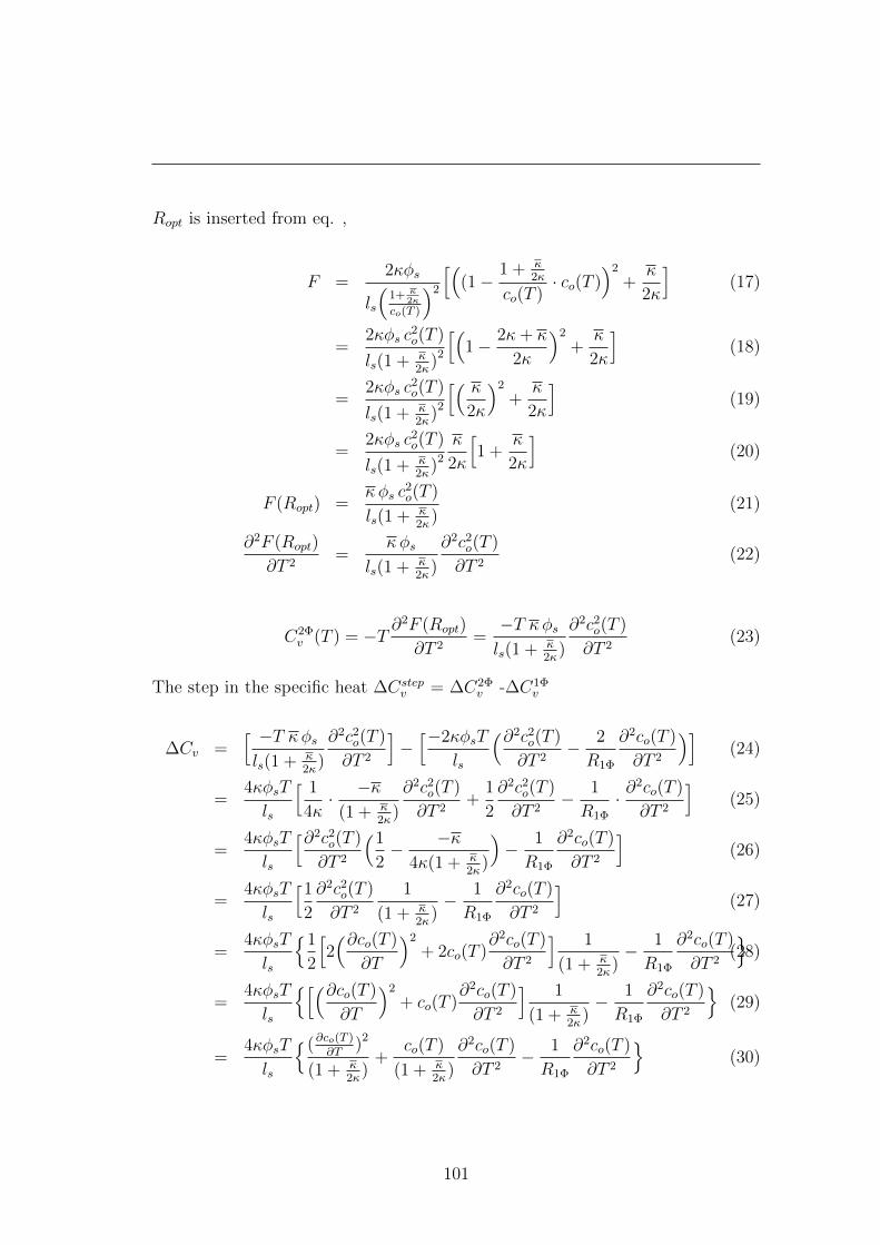
Ropt is inserted from eq. ,

F =2κφs

ls

(1+ κ

2κ

co(T )

)2

[((1−

1 + κ2κ

co(T )· co(T )

)2

+κ

2κ

](17)

=2κφs c

2o(T )

ls(1 + κ2κ

)2

[(1− 2κ+ κ

2κ

)2

+κ

2κ

](18)

=2κφs c

2o(T )

ls(1 + κ2κ

)2

[( κ2κ

)2

+κ

2κ

](19)

=2κφs c

2o(T )

ls(1 + κ2κ

)2

κ

2κ

[1 +

κ

2κ

](20)

F (Ropt) =κφs c

2o(T )

ls(1 + κ2κ

)(21)

∂2F (Ropt)

∂T 2=

κφsls(1 + κ

2κ)

∂2c2o(T )

∂T 2(22)

C2Φv (T ) = −T ∂

2F (Ropt)

∂T 2=−T κφsls(1 + κ

2κ)

∂2c2o(T )

∂T 2(23)

The step in the specific heat ∆Cstepv = ∆C2Φ

v -∆C1Φv

∆Cv =[ −T κφsls(1 + κ

2κ)

∂2c2o(T )

∂T 2

]−[−2κφsT

ls

(∂2c2o(T )

∂T 2− 2

R1Φ

∂2co(T )

∂T 2

)](24)

=4κφsT

ls

[ 1

4κ· −κ

(1 + κ2κ

)

∂2c2o(T )

∂T 2+

1

2

∂2c2o(T )

∂T 2− 1

R1Φ

· ∂2co(T )

∂T 2

](25)

=4κφsT

ls

[∂2c2o(T )

∂T 2

(1

2− −κ

4κ(1 + κ2κ

)

)− 1

R1Φ

∂2co(T )

∂T 2

](26)

=4κφsT

ls

[1

2

∂2c2o(T )

∂T 2

1

(1 + κ2κ

)− 1

R1Φ

∂2co(T )

∂T 2

](27)

=4κφsT

ls

{1

2

[2(∂co(T )

∂T

)2

+ 2co(T )∂2co(T )

∂T 2

] 1

(1 + κ2κ

)− 1

R1Φ

∂2co(T )

∂T 2

}(28)

=4κφsT

ls

{[(∂co(T )

∂T

)2

+ co(T )∂2co(T )

∂T 2

] 1

(1 + κ2κ

)− 1

R1Φ

∂2co(T )

∂T 2

}(29)

=4κφsT

ls

{(∂co(T )∂T

)2

(1 + κ2κ

)+

co(T )

(1 + κ2κ

)

∂2co(T )

∂T 2− 1

R1Φ

∂2co(T )

∂T 2

}(30)

101

=4κφsT

ls

{(∂co(T )∂T

)2

(1 + κ2κ

)+

1

Ropt

∂2co(T )

∂T 2− 1

R1Φ

∂2co(T )

∂T 2

}(31)

Then,

∆Cv =4κφsT

ls

{∂2co(T )

∂T 2

[R1Φ −Ropt

RoptR1Φ

]+

(∂co(T )∂T

)2

1 + κ2κ

}(32)

102

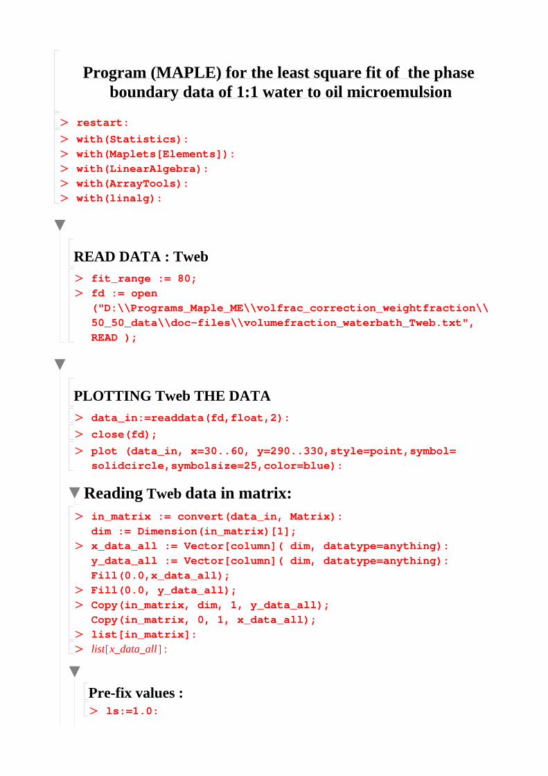
O

O

O

O

O

O

O

O

O

O

O

O

O

O

O

O

O

O

Program (MAPLE) for the least square fit of the phase boundary data of 1:1 water to oil microemulsion

restart:

with(Statistics):with(Maplets[Elements]):with(LinearAlgebra):with(ArrayTools):with(linalg):

READ DATA : Tweb fit_range := 80;fd := open("D:\\Programs_Maple_ME\\volfrac_correction_weightfraction\\50_50_data\\doc-files\\volumefraction_waterbath_Tweb.txt", READ );

PLOTTING Tweb THE DATAdata_in:=readdata(fd,float,2):

close(fd);

plot (data_in, x=30..60, y=290..330,style=point,symbol=solidcircle,symbolsize=25,color=blue):

Reading Tweb data in matrix:in_matrix := convert(data_in, Matrix):dim := Dimension(in_matrix)[1];x_data_all := Vector[column]( dim, datatype=anything):y_data_all := Vector[column]( dim, datatype=anything):Fill(0.0,x_data_all); Fill(0.0, y_data_all);Copy(in_matrix, dim, 1, y_data_all);Copy(in_matrix, 0, 1, x_data_all);list[in_matrix]:list x_data_all :

Pre-fix values : ls:=1.0:

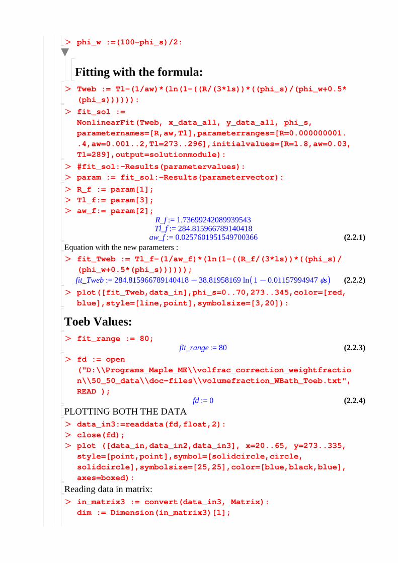
O

O O

O

O

O

O

O

O

(2.2.4)

(2.2.1)

O

O

O

O

(2.2.2)

O O

(2.2.3)

O

phi_w :=(100-phi_s)/2:

Fitting with the formula:Tweb := Tl-(1/aw)*(ln(1-((R/(3*ls))*((phi_s)/(phi_w+0.5*(phi_s)))))):

fit_sol := NonlinearFit(Tweb, x_data_all, y_data_all, phi_s, parameternames=[R,aw,Tl],parameterranges=[R=0.000000001..4,aw=0.001..2,Tl=273..296],initialvalues=[R=1.8,aw=0.03,Tl=289],output=solutionmodule):

#fit_sol:-Results(parametervalues):param := fit_sol:-Results(parametervector):

R_f := param[1];Tl_f:= param[3];aw_f:= param[2];

R_f := 1.73699242089939543Tl_f := 284.815966789140418

aw_f := 0.0257601951549700366Equation with the new parameters :

fit_Tweb := Tl_f-(1/aw_f)*(ln(1-((R_f/(3*ls))*((phi_s)/(phi_w+0.5*(phi_s))))));fit_Tweb := 284.815966789140418K38.81958169 ln 1K0.01157994947 φsplot([fit_Tweb,data_in],phi_s=0..70,273..345,color=[red,blue],style=[line,point],symbolsize=[3,20]):

Toeb Values:fit_range := 80;

fit_range := 80fd := open("D:\\Programs_Maple_ME\\volfrac_correction_weightfraction\\50_50_data\\doc-files\\volumefraction_WBath_Toeb.txt",READ );

fd := 0PLOTTING BOTH THE DATA

data_in3:=readdata(fd,float,2):close(fd);plot ([data_in,data_in2,data_in3], x=20..65, y=273..335,style=[point,point],symbol=[solidcircle,circle,solidcircle],symbolsize=[25,25],color=[blue,black,blue],axes=boxed):

Reading data in matrix:in_matrix3 := convert(data_in3, Matrix):dim := Dimension(in_matrix3)[1];

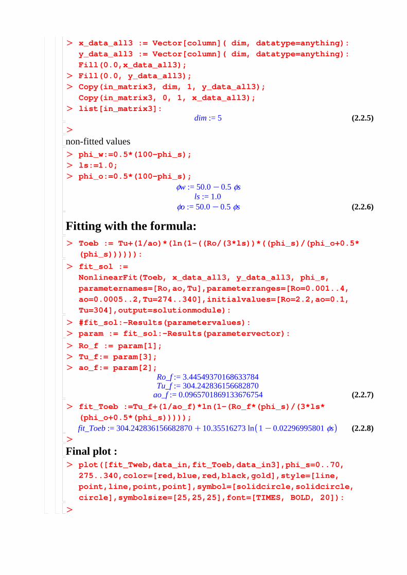
O

O

O

O

O (2.2.8)

O

O

O

O

O

O

O

O

O

O

O

(2.2.6)

(2.2.7)

O

O

O

(2.2.5)

x_data_all3 := Vector[column]( dim, datatype=anything):y_data_all3 := Vector[column]( dim, datatype=anything):Fill(0.0,x_data_all3); Fill(0.0, y_data_all3);Copy(in_matrix3, dim, 1, y_data_all3);Copy(in_matrix3, 0, 1, x_data_all3);list[in_matrix3]:

dim := 5

non-fitted valuesphi_w:=0.5*(100-phi_s);ls:=1.0;phi_o:=0.5*(100-phi_s);

φw := 50.0K0.5 φsls := 1.0

φo := 50.0K0.5 φs

Fitting with the formula:Toeb := Tu+(1/ao)*(ln(1-((Ro/(3*ls))*((phi_s)/(phi_o+0.5*(phi_s)))))):

fit_sol := NonlinearFit(Toeb, x_data_all3, y_data_all3, phi_s, parameternames=[Ro,ao,Tu],parameterranges=[Ro=0.001..4,ao=0.0005..2,Tu=274..340],initialvalues=[Ro=2.2,ao=0.1,Tu=304],output=solutionmodule):

#fit_sol:-Results(parametervalues):param := fit_sol:-Results(parametervector):

Ro_f := param[1];Tu_f:= param[3];ao_f:= param[2];

Ro_f := 3.44549370168633784Tu_f := 304.242836156682870

ao_f := 0.0965701869133676754fit_Toeb :=Tu_f+(1/ao_f)*ln(1-(Ro_f*(phi_s)/(3*ls*(phi_o+0.5*(phi_s)))));fit_Toeb := 304.242836156682870C10.35516273 ln 1K0.02296995801 φs

Final plot : plot([fit_Tweb,data_in,fit_Toeb,data_in3],phi_s=0..70,275..340,color=[red,blue,red,black,gold],style=[line,point,line,point,point],symbol=[solidcircle,solidcircle,circle],symbolsize=[25,25,25],font=[TIMES, BOLD, 20]):

References

[1] Hakan Wennerstrom D. Fennell Evans. The Colloidal Domain : Where

Physics, Chemistry, Biology, and Technology Meet. Wiley-VCH, 1999. x,

8, 9

[2] M Kahlweit and R Strey. Phase behavior of ternary systems of the type h20-

oil-nonionic amphiphile (microemulsions). Angew. Chem. Int. Ed. Engl., 24:

654–668, 1985. xi, 19, 20, 23

[3] M Daoud and C.E. Williams. Soft Matter Physics. Springer, 1999. 2, 3, 8,

14

[4] J Israelachvili. Intermolecular and Surface Forces (second edition). Academic

Press, 1991. 3, 8, 88

[5] Tadros F. Applied Surfactant : Priciples and Applications. Wiley-VCH,

2005. 3

[6] J. F. Goodman J. M. Corkill and S. P Harrold. Thermodynamics of mi-

cellization of non-ionic detergents. Trans. Faraday Soc., 60:202, 1964. 3,

70

[7] H.-F. Eicke. Surfactants in nonpolar solvents. aggregation and micellization.

Topics in Current Chemistry, 87:85–145, 1980. 5, 6, 7

[8] Toshihiro Jin-Noa Kijiro Kon-Noa and Ayao Kitahara. Journal of Colloid

and Interface Science, 49:3, 1974. 5

103

REFERENCES

[9] A KITAHARA and K KON-NO. Micelle Formation in Nonaqueous Me-

dia, Colloidal Dispersions and Micellar Behavior. ACS Symposium Series;

American Chemical Society, 1975. 5

[10] D. O Shah. Micelles, Microemulsions, and Monolayers. Science and Tech-

nology, CRC Press, 1998. 6

[11] Martin J. Schick. Nonionic surfactants: Physical chemistry (Surfactant sci-

ence series, Volume 23). Marcel Dekker, Inc., New York and Basel, 1987.

6

[12] Nagarajan R Ruckenstein, E. Aggregation of amphiphiles in nonaqueous

media. The Journal of Physical Chemistry, 84:1349–1358, 1980. 6

[13] C.R Singleterry. Micelle formation and solubilization in nonaqueous solvents.

Journal of the American Oil Chemists’ Society, 32:446–452, 1955. 6

[14] M.; Picot C. Ravey, J. C.; Buzier. Micellar structures of nonionic surfactants

in apolar media. Journal of Colloid and Interface Science, 97:9–25, 1984. 7

[15] R Strey. Water-nonionic surfactant systems and the effect of additives.

BERICHTE DER BUNSEN-GESELLSCHAFT-PHYSICAL CHEMISTRY

CHEMICAL PHYSICS, 100:182–189, 1996. 8

[16] Rosen M. J. Surfactants and interfacial phenomena (third edition). Wiley

and Sons, Inc., New York, 2004. 10

[17] W Helfrich. Elastic properties of lipid bilayerstheory and possible experi-

ments. Z. Naturforsch. C, 28:693–703, 1973. 13, 24

[18] U. Olsson and H. Wennerstrom. Globular and bicontinuous phases of non-

ionic surfactant films. Advances in Colloid and Interface Science, 49:113–146,

1994. 13, 32, 37

[19] J. Daicic, U. Olsson, and H. Wennerstrm. Phase equilibria of balanced

microemulsions. Langmuir, 11(7):2451–2458, 1995. URL www.scopus.com.

Cited By (since 1996): 35. 13, 37

104

REFERENCES

[20] B.Lindman and H. Wennerstrom. Topics in Current Chemistry : Micelles.

Amphiphile Aggregation in Aqueous Solution. Springer-Verlag, 1980. 15

[21] Nabil Naouli and Henri L. Rosano. Chapter 7. In Design of Single Surfactant

Microemulsion Micro/Nanoencapsulation of Active Food Ingredients, volume

1007 of ACS Symposium Series, pages 116–130, 2009. 17

[22] T.P. Hoar and J.H Schulman. Transparent water-in-oil dispersions; the oleo-

pathic hydromicelle. Nature, 152:102–103, 1943. 17

[23] J.H. Schulman and D.P. Riley. X-ray investigation of the structure of trans-

parent oilwater disperse systems.1. J. Colloid Sci., 3:383405, 1948. 17

[24] J.E. Bowcott and J.H. Schulman. Emulsions- control of droplet size and

phase continuity in transparent oilwater dispersions stabilized with soap and

alcohol. Z. Electrochem., 59:283–290, 1955. 17

[25] J.H. Schulman and J.A. Friend. Light scattering investigation of the struc-

ture of transparent oilwater disperse systems. 2. J. Colloid Sci., 4:497–509,

1949. 17

[26] Stoeckenius W. Schulman, J.H. and L.M. Prince. Mechanism of formation

and structure of microemulsions by electron microscopy. J. Phys. Chem., 63:

1677–1680, 1959. 17

[27] M. Kahlweit. The phase behaviour of the type h2ooilnonionic surfactant-

electrolyte. J. Colloid Interface Sci., 90:197202, 1982. 18

[28] Lessner E. Kahlweit, M. and R. Strey. Influence of the properties of

the oil and the surfactant on the phase-behaviour of systems of the type

h2ooilnonionic surfactant. J. Phys. Chem., 87:50325040, 1983. 18

[29] T Sottmann and R Strey. Ultralow interfacial tensions in water-n-alkane-

surfactant systems. J. Chem. Phys., 106:20, 1997. 18, 79, 80

[30] H.L. Rosano and M. Clausse. Microemulsion Systems : Surfactant Science

Series; Volume 24. Marcel Dekker, New York, 1987. 19

105

REFERENCES

[31] PA Winsor. Hydrotropy, solubilisation and related emulsification processes.

Trans. Faraday Soc., 44:376–398, 1948. 20, 21

[32] R ; FIRMAN P KAHLWEIT, M; STREY. Search for tricritical points in

ternary-systems - water oil nonionic amphiphile. JOURNAL OF PHYSICAL

CHEMISTRY, 90:671–677, 1986. 21, 22

[33] G. Gompper and M. Schick. Self-assembling amphiphilic systems : in : Phase

Transitions and Critical Phenomena, volume 16. Academic Press, London,

1994. 22, 24, 25

[34] R. Strey M. Kahlweit and G. Busse. Microemulsions: A qualitative thermo-

dynamic approach. J. Phys. Chem., 94:3881–3894, 1990. 23, 96

[35] 101 (1999) Doris Vollmer rule. How to calculate phase diagrams for mi-

croemulsions - a simple rule. Fett/Lipid, 101:379–388, 1999. 23, 34, 77,

96

[36] T. VanDinter O. Desrosier and S. K. Saunders. Can. J. Chem., 62:56, 1984.

24

[37] G. Perron G. Roux and J.E. Desnoyers. J. Solution Chem., 7:639, 1978. 24

[38] M. Schick and Wei-Heng Shih. Simple microscopic model of a microemulsion.

Phys. Rev. Lett., 59:1205–1208, Sep 1987. doi: 10.1103/PhysRevLett.59.

1205. URL http://link.aps.org/doi/10.1103/PhysRevLett.59.1205.

24, 27

[39] B. Widom. Ii. theoretical modeling: An introduction. Berichte der Bunsen-

gesellschaft fr physikalische Chemie, 100(3):242–251, 1996. ISSN 0005-9021.

doi: 10.1002/bbpc.19961000310. URL http://dx.doi.org/10.1002/bbpc.

19961000310. 24, 27

[40] G Gompper. Ginzburg-landau theories of ternary amphiphilic systems.

BERICHTE DER BUNSEN-GESELLSCHAFT-PHYSICAL CHEMISTRY

CHEMICAL PHYSICS, 100:264–271, 1996. 24

106

REFERENCES

[41] D. Roux M. Gelbart, editor. Micelles, Membranes, Microemulsions and

Monolayers. Springer, Berlin, 1995. 24

[42] Y. Talmon and S. Prager. Statistical thermodynamics of phase equilibria in

microemulsions. J. Chem. Phys., 69:2984, 1978. 25

[43] E. Ruckenstein and J. Chi. J. Chem. Sot. Faraday Trans., 271:1690, 1975.

25

[44] P.G. de Gennes and C. Taupin. J. Phys. Chem., 86:2294, 1982. 25, 26, 28

[45] P. Levinson J. Jouffroy and P.G. de Gennes. J. Phys. (France), 43:1241,

1982. 25

[46] B. Widom. J. Chem. Phys., 81:1030, 1984. 25

[47] D. Andelman. M. E. Cates. D. Roux and S. A. Safran. J. Chem. Phys., 87:

7229, 1987. 25, 29

[48] J. H. Schulman and J. B. Montagne. Formation of microemulsions by amino

alkyl alcohols. Annals of the New York Academy of Sciences, 92:366–371,

1961. 26

[49] M. Ellerby H. Reiss and J. A. Manzanares. Configurational entropy of mi-

croemulsions: The fundamental length scale. J. Chem. Phys., 99:9930, 1993.

26

[50] M. Kahlweit and H. Reiss. Langmuir, 7:2929, 1991. 26

[51] J. Jen M. Kahlweit and G. Busse. J. Phys. Chem., 97:6917, 1992. 26

[52] Wheeler JC and B Widom. Phase transitions and critical points in a model

3-component system. J. Am. Chem. Soc., 90:3064, 1968. 27

[53] A. Robledo. Exact thermodynamic correspondence between a lattice model

microemulsion and simpler spin systems. EPL (Europhysics Letters), 1(6):

303, 1986. URL http://stacks.iop.org/0295-5075/1/i=6/a=006. 27

107

REFERENCES

[54] A. Robledo. Spin ising transcription of a lattice model of micellar solutions.

Physical Review A, 36(8):4067–4071, 1987. URL www.scopus.com. Cited By

(since 1996): 4. 27

[55] M. W. Matsen and D. E. Sullivan. Lattice model for surfactants in solution.

Phys. Rev. A, 41:2021–2030, Feb 1990. doi: 10.1103/PhysRevA.41.2021.

URL http://link.aps.org/doi/10.1103/PhysRevA.41.2021. 27

[56] W. Helfrich. Z. Naturforsch. C, 33a:305, 1978. 28

[57] S. A. Safran, L. A. Turkevich, and P. Pincus. Cylindrical microemulsions: a

polymer-like phase ? J. Physique Lett, 45:L–64, 1984. 28, 32, 37

[58] J. Vollmer D. Vollmer and R. Strey. Phys. Rev. E, 54:3028, 1996. 28, 37

[59] H. Bagger-Jrgensen, U. Olsson, and K. Mortensen. Langmuir, 12:4057, 1996.

29

[60] D. Vollmer, J. Vollmer, R. Strey, H.-G. Schmidt, and G. Wolf. Journal of

Thermal Analysis, 51:9–27, 1998. 29, 36, 37

[61] R Strey. Microemulsion microstructure and interfacial curvature. Colloid &

Polymer Science, 272:1005–1019, 1994. 32

[62] R. Strey D. Vollmer and J. Vollmer. Oscillating phase separation in mi-

croemulsions. i.experimental observation. J. Chem. Phys., 107:3619, 1997.

36, 37

[63] J Vollmer D. Vollmer and A. J. Wagner. Oscillatory kinetics of phase sep-

aration in a binary mixture under constant heating. Phys. Chem. Chem.

Phys., 4:1380–1385, 2002. 36

[64] D. Vollmer and P. Ganz. Microcalorimetric investigation of the upper phase

boundary of water-in-oil microemulsions;. J. Chem. Phys., 103:11, 1995. 36

[65] Strey R Vollmer J, Vollmer D. J chem Phys, 107:3627, 1997. 36

[66] StreyR Vollmer D, Vollmer J. EuroPhys Lett, 39:245, 1997. 36

108

REFERENCES

[67] D. Vollmer. Phase separation in microemulsions: stepwise change of the

droplet size. Colloid Polym Sci, 278:728–735, 2000. 36, 37

[68] Vollmer J and Vollmer D. Cascade nucleation in the phase separation of

amphiphilic mixtures. Faraday Discuss., 112:51–62, 1999. 37

[69] S. A. Safran and L. A. Turkevich. Phase diagrams for microemulsions. Phys.

Rev. Lett., 50:1930–1933, Jun 1983. doi: 10.1103/PhysRevLett.50.1930. URL

http://link.aps.org/doi/10.1103/PhysRevLett.50.1930. 37

[70] S. A. Safran. Microemulsions: an ensemble of fluctuating interfaces : Struc-

ture and Dynamics of Strongly Interacting Colloids and Supramolecular Ag-

gregates in Solution. Kluwer Academic Publishers, Dordrecht, 1992. 37

[71] P. Lecomte du Noy. A new apparatus for measuring surface tension. The

Journal of General Physiology, 1(5):521–524, 1919. doi: 10.1085/jgp.1.5.521.

URL http://jgp.rupress.org/content/1/5/521.short. 53

[72] 68 3 (1983) Shinoda, K. Prog.Colloid Polym. sci., 68:3, 1983. 58

[73] Tharwat F. Tadros. Self-organised Surfactant Structures. Wiley-VCH, 2010.

58

[74] Schubert K.-V and Kaler E.W. Nonionic microemulsions. Ber. Bunsenges.

Phys. Chem., 100:190–205, 1996. 79, 80, 93

[75] Strey R Hasse D et al. Kahlweit, M. J. Colloid Interface Sci., 118:436–453,

1987. 79, 80, 93

[76] T. Foster. Microemulsions as compartmentalised reaction media : structural

characterisation of water-in-oil microemulsions. PhD thesis, University of

Cologne, 2007. 85

109