Microeconomics Supply Producing Producing efficiently Maximizing profit.
27
Microeconomics Supply Producing Producing efficiently Maximizing profit
-
Upload
allen-richard -
Category
Documents
-
view
223 -
download
0
Transcript of Microeconomics Supply Producing Producing efficiently Maximizing profit.

Microeconomics
SupplyProducing
Producing efficientlyMaximizing profit

A note on abstractions• The firm as a productive entity that transforms inputs into outputs
– As if there is one manager who acts like an owner, allocating resources to maximize profit
– Like the firm was a plant producing a single product– Clear parallel with choice theory (actually just an extension of choice
theory)– Abstracts away most of the details, but very useful in explaining
production and pricing decisions– Sets benchmark cases for comparison with more complicated scenarios
• The firm as an organization in which production requires the coordination of decision-making and implementation– Who has what authority among the many managers?– How to motivate managers to act like owners?– How to monitor and evaluate performance?– Descriptive, but messy

ProducingConsumption is the sole end and purpose
of all production; and the interest of the producer ought to be attended to, only so
far as it may be necessary for promoting that of the consumer.
Adam Smith, Wealth of Nations

Mapping inputs to outputs
• A production function gives the maximum output for a given set of inputs
• The production function represents the firm’s technological constraint
• Focus on two inputs, labor (L) and capital (K)
• What are the relevant units of L an K?
),...,( 1 nxxfQ
),( KLfQ

Measuring inputs
• Inputs measured as flows• What are the prices of these flows?– Wage rate for labor hours– “Rental” rate for capital flows
• How to think about the rental rate when capital equipment is purchased?– Difference between current value and purchase price can
be used to calculate an implicit rental rate– Rental rate can be approximated by the interest rate
because it captures opportunity cost of tying up resources in capital equipment for a given period

Types of production functions
• What is a reasonable specification for f ?– Additive inputs? – Multiplicative inputs? – Inputs used in fixed proportions?
• Implications – suppose L and K “interact”– Capital complemented by skilled labor– Optimal skill level rises with capital-labor ratio

Productivity at the margin
• An input’s marginal product is its effect on output when another unit is employed, holding other inputs constant
• What pattern do you expect MP to follow?• When will the MP of one input depend on how
other inputs are used? (The answer depends on the form of f.)
K
QMP
L
QMP KL
,
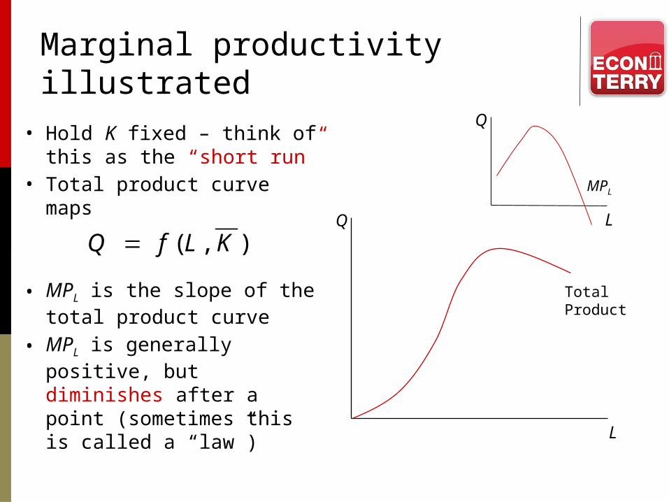
Marginal productivity illustrated
• Hold K fixed – think of this as the “short run”
• Total product curve maps
• MPL is the slope of the total product curve
• MPL is generally positive, but diminishes after a point (sometimes this is called a “law”)
L
Q
Total Product
),( KLfQ L
Q
MPL

Returns to scale
• In the long run, the firm can adjust all inputs – the entire scale of the business
• What happens to output when all inputs are changed proportionately?
• The answer is in the returns to scale
• Why might you be skeptical about persistent DRS?
),( KLf = λQ implies constant returns to scale (CRS)> λQ implies increasing returns to scale (IRS)< λQ implies decreasing returns to scale (DRS)

Producing efficiently
All accounting information was Sarah’s, and nothing left her office.
Airtex AviationHBS case 9-800-269

From production to cost
• To produce efficiently means to produce at least cost
where w is the wage rate and r is the price of capital
• The production function is the constraint in achieving that goal
• The cost function gives the minimum cost of producing a given level of output, Q
),(..)min( KLfQtsrKwL
),,( QrwCC

Costs in the short run
• Distinguish between variable and fixed costs
• What costs/inputs are fixed in your business?• Average costs
• Marginal cost
FCQVCQC )()(
AFCAVCATC
Q
FC
Q
QVC
Q
QC
)()(
Q
QVCQMCMC
)(
)(

Cost curves in the short run
Q
C
• Q
• CTC
TVC
AVCATCMC
minimum values
AFC
These stylized short-run curves capture the fundamental relationshipsbetween cost concepts. Two questions: (1) How are they related to the production concepts? (2) How do you account for their shapes?
Cost curves in the short run – summary• The AVC curve may initially slope down, but will
eventually rise as long as there are fixed inputs that constrain production
• The ATC curve is U-shaped, falling initially because of declining AFC, then rising because of increasing AVC
• The MC curve may initially slope down, but will eventually rise due to diminishing marginal productivity– The MC curve lies below the average cost curves when
average costs are decreasing and above them when average costs are increasing
– MC = ATC and AVC at their minimum values

An illustration with Gary Geek
• Gary Geek is in the computer repair business with a cost function that looks like this
• This means his MC of computer repair is 4Q• Let’s plot Gary’s MC curve, along with his ATC
and AVC curves
2002)( 2 QQC

Gary Geek’s data and plotsGary Geek's Cost Schedule and Curves
Q C(Q) MC AVC ATC1 202 4 2 202.004 232 16 8 58.009 362 36 18 40.22
16 712 64 32 44.5025 1450 100 50 58.0036 2792 144 72 77.56
0
50
100
150
200
250
1 4 9 16 25 36
MC
AVC
ATC

Costs in the long run
• Let’s say the short run is whatever period K must remain fixed
• A firm should be able to do at least as well when K is adjustable as when it is fixed
• Cost in the long run should be no greater than cost in the short run
• What does this imply about the long-run AC curve?

Cost curves in the long run
Q
LRMC
• The short-run ATC curve (SRAC) gives the lowest unit cost for a given capital stock
• The long-run AC (LRAC) curve is the envelope of all possible short-run ATC curves
• Why might the LRAC be U-shaped?– Under CRS, the LRAC curve is
horizontal (AC is constant) and LRAC = LRMC
– CRS characterizes the typical firm in a mature, competitive industry
– Remember the replication argument
CLRAC
minimum LRAC
SRAC
Efficient scale
The SRAC curve that is tangent to the LRAC at its minimum point reflects the efficient scale of production
Efficient scale and shifts in LRAC curves
• Efficient scale– Role of competitive markets – Threat of entry– When efficient scale is small relative to industry
demand, the number of competitors will be large• Shifting cost curves– Technology– Input prices– Learning (from cumulative production)

Maximizing profit
No profit grows where is no pleasure ta'en; In brief, sir, study
what you most affect.
William Shakespeare, Taming of the Shrew

The meaning of profit
• For profit to have economic meaning– All inputs must be counted– All inputs must be valued at their market prices (which
reflect their opportunity costs)– Opportunity cost – input’s value if purchased “now”
• Differences between opportunity and historical costs– Cost of durable inputs (e.g., depreciation, internal
finance)– Cost of inputs not purchased from the market (e.g.,
proprietor’s income, the farmer’s land)

22
Sunk costs• A sunk cost is a payment that cannot be recovered• Sunk costs should not influence decision-making
• Consider this scenario: You bought a ticket to the U2 show last month. You paid $75. When you arrive at the arena you discover the ticket is lost. What do you do?– Suppose you can buy a comparable ticket from a broker for the
same price you originally paid. Do you buy it?– Suppose instead that when you arrive at the arena you discover
you lost $75 cash. Do you sell your ticket?

Profit and stock-market value
• In a world of perfect certainty, maximizing profit and stock-market value is the same thing – think of a corporation– Shares are ownership claims– Dividends are an owner’s share of the profits– Share price is the PV of the dividend stream
• With uncertainty, maximizing profit loses meaning – Hard to state in advance what attitude managers should have
toward risk– Maximizing stock-market value still makes sense because it
makes the owners as well off as possible• Nevertheless, we will stick with the profit-maximizing
objective

The problem and the solution
• The problem – choose Q to
• The solution – produce Q*, the level at which the benefit and cost of the last unit are equal
)]([max QCPQ
MCMR
MC$
Q*Q
MR > MC MR < MC
MR
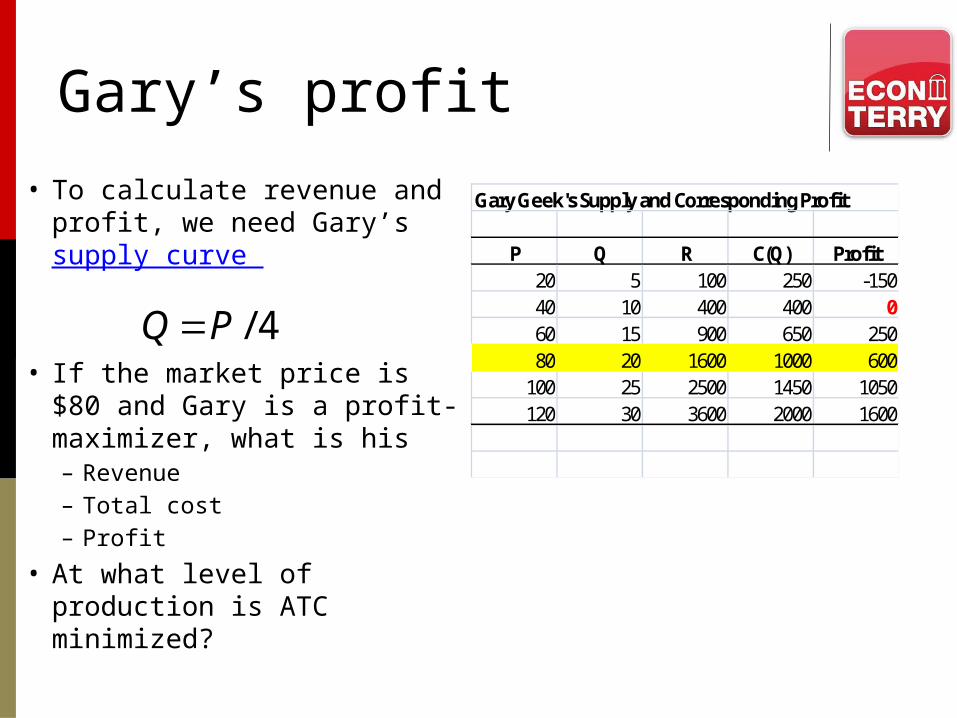
Gary’s profit
• To calculate revenue and profit, we need Gary’s supply curve
• If the market price is $80 and Gary is a profit-maximizer, what is his– Revenue– Total cost– Profit
• At what level of production is ATC minimized?
4/PQ
Gary Geek's Supply and Corresponding Profit
P Q R C(Q) Profit20 5 100 250 -15040 10 400 400 060 15 900 650 25080 20 1600 1000 600
100 25 2500 1450 1050120 30 3600 2000 1600

Rule for hiring inputs
• How would you translate the rule for profit-maximizing into optimal hiring?
• Think about labor (of a single type)– What is the benefit of an extra worker hour?– What is the cost?
• In general, hire inputs up to the point
• If you profit maximize, you will hire optimallyMCMRPMRMP
Takeaways• Marginal products eventually fall because of short-run constraints• Returns to scale tell you what can happen when all of the short-run
constraints are removed• Producing efficiently is producing at least cost• Cost functions tell you how to do that• Cost curves are derived from cost functions• Changes in technology and input prices shift cost curves; so does
learning• Marginal cost eventually rises in the short run for the same reason
marginal products fall• Profit has economic meaning only if defined in terms of opportunity cost• Sunk costs are sunk• You maximize profit the same way you choose optimally – by equating
costs and benefits at the margin