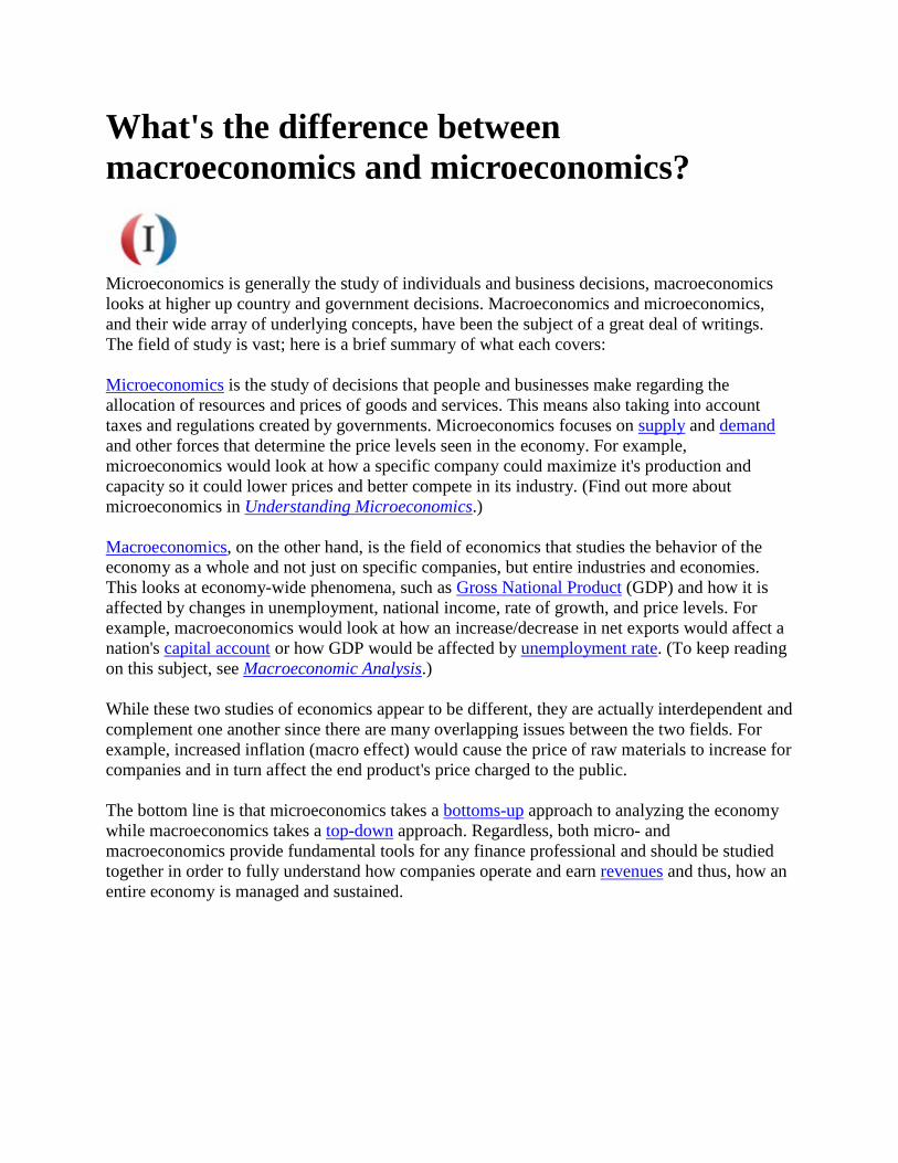
What's the difference between macroeconomics and microeconomics?

Microeconomics is generally the study of individuals and business decisions, macroeconomics looks at higher up country and government decisions. Macroeconomics and microeconomics, and their wide array of underlying concepts, have been the subject of a great deal of writings. The field of study is vast; here is a brief summary of what each covers: Microeconomics is the study of decisions that people and businesses make regarding the allocation of resources and prices of goods and services. This means also taking into account taxes and regulations created by governments. Microeconomics focuses on supply and demand and other forces that determine the price levels seen in the economy. For example, microeconomics would look at how a specific company could maximize it's production and capacity so it could lower prices and better compete in its industry. (Find out more about microeconomics in Understanding Microeconomics.) Macroeconomics, on the other hand, is the field of economics that studies the behavior of the economy as a whole and not just on specific companies, but entire industries and economies. This looks at economy-wide phenomena, such as Gross National Product (GDP) and how it is affected by changes in unemployment, national income, rate of growth, and price levels. For example, macroeconomics would look at how an increase/decrease in net exports would affect a nation's capital account or how GDP would be affected by unemployment rate. (To keep reading on this subject, see Macroeconomic Analysis.) While these two studies of economics appear to be different, they are actually interdependent and complement one another since there are many overlapping issues between the two fields. For example, increased inflation (macro effect) would cause the price of raw materials to increase for companies and in turn affect the end product's price charged to the public. The bottom line is that microeconomics takes a bottoms-up approach to analyzing the economy while macroeconomics takes a top-down approach. Regardless, both micro- and macroeconomics provide fundamental tools for any finance professional and should be studied together in order to fully understand how companies operate and earn revenues and thus, how an entire economy is managed and sustained.

In macroeconomics:

• There are no: o Substitute goods or services. o Complimentary goods and services. o Normal goods and services. o Inferior goods and services

=>There are just “aggregate goods and services”. • Ceteris paribus is not an issue in macroeconomics. • We do not care why consumers make individual choices. We are not concerned with:

o Price elasticity of demand. o Budget constraints of consumers. o Marginal utility of consumers.

• Firms (producers) are simply firms (producers). We do not worry about whether a firm is:

o A perfect competitor. o A monopolist. o In monopolistic competition. o An oligopolist.

• We do not concern ourselves with the size or behavior of the firm in macroeconomics. • We still emphasize the concept of “opportunity costs”, but we now apply that concept to

whole economies or societies. • You will not hear the phrases “marginal cost” or “marginal revenue”. These two

concepts are not an issue in macroeconomics.

Micro economics is concerned with:

• Supply and demand in individual markets • Individual consumer behaviour. e.g. Consumer choice theory • Individual labour markets – e.g. demand for labour, wage determination • Externalities arising from production and consumption.

• Monetary / fiscal policy. e.g. what effect does interest rates have on whole economy?

Macro economics is concerned with

• Reasons for inflation, and unemployment • Economic Growth • International trade and globalization • Reasons for differences in living standards and economic growth between countries. • Government borrowing

Economics Basics: Elasticity Filed Under » Alfred Marshall Macroeconomics, Microeconomics, Monetary Policy, Macroeconomics, Microeconomics, Monetary Policy, Alfred Marshall The degree to which a demand or supply curve reacts to a change in price is the curve's elasticity. Elasticity varies among products because some products may be more essential to the consumer. Products that are necessities are more insensitive to price changes because consumers would continue buying these products despite price increases. Conversely, a price increase of a good or service that is considered less of a necessity will deter more consumers because the opportunity cost of buying the product will become too high. A good or service is considered to be highly elastic if a slight change in price leads to a sharp change in the quantity demanded or supplied. Usually these kinds of products are readily available in the market and a person may not necessarily need them in his or her daily life. On the other hand, an inelastic good or service is one in which changes in price witness only modest changes in the quantity demanded or supplied, if any at all. These goods tend to be things that are more of a necessity to the consumer in his or her daily life. To determine the elasticity of the supply or demand curves, we can use this simple equation:

Elasticity = (% change in quantity / % change in price)

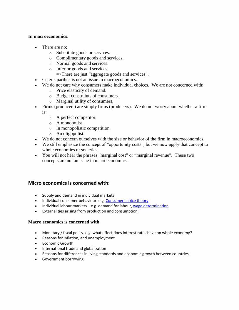
If elasticity is greater than or equal to one, the curve is considered to be elastic. If it is less than one, the curve is said to be inelastic. As we mentioned previously, the demand curve is a negative slope, and if there is a large decrease in the quantity demanded with a small increase in price, the demand curve looks flatter, or more horizontal. This flatter curve means that the good or service in question is elastic.

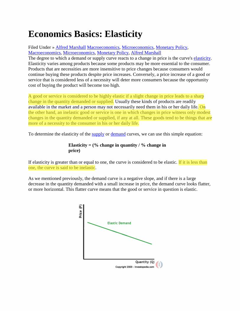
Meanwhile, inelastic demand is represented with a much more upright curve as quantity changes little with a large movement in price.

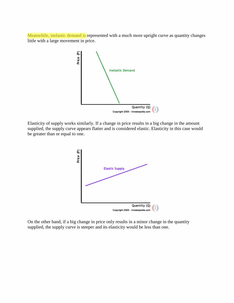
Elasticity of supply works similarly. If a change in price results in a big change in the amount supplied, the supply curve appears flatter and is considered elastic. Elasticity in this case would be greater than or equal to one.

On the other hand, if a big change in price only results in a minor change in the quantity supplied, the supply curve is steeper and its elasticity would be less than one.

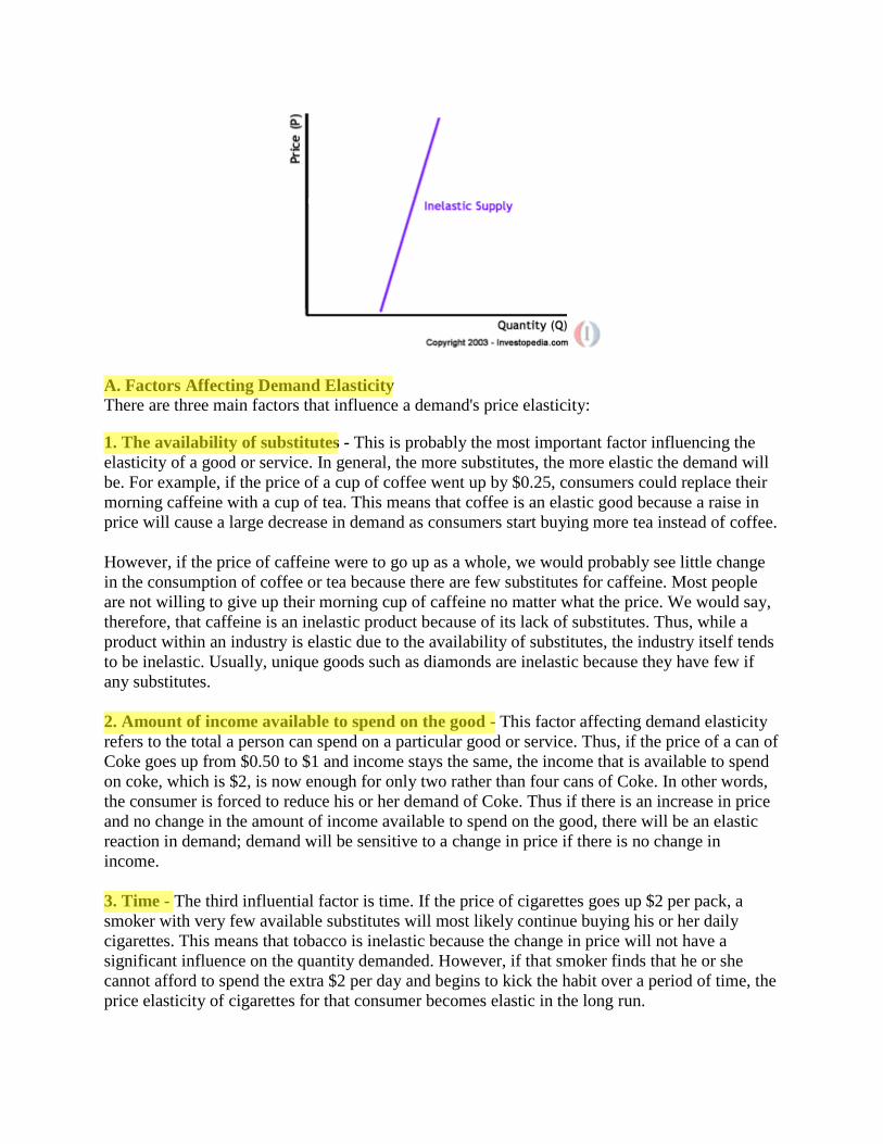
A. Factors Affecting Demand Elasticity There are three main factors that influence a demand's price elasticity:

1. The availability of substitutes - This is probably the most important factor influencing the elasticity of a good or service. In general, the more substitutes, the more elastic the demand will be. For example, if the price of a cup of coffee went up by $0.25, consumers could replace their morning caffeine with a cup of tea. This means that coffee is an elastic good because a raise in price will cause a large decrease in demand as consumers start buying more tea instead of coffee. However, if the price of caffeine were to go up as a whole, we would probably see little change in the consumption of coffee or tea because there are few substitutes for caffeine. Most people are not willing to give up their morning cup of caffeine no matter what the price. We would say, therefore, that caffeine is an inelastic product because of its lack of substitutes. Thus, while a product within an industry is elastic due to the availability of substitutes, the industry itself tends to be inelastic. Usually, unique goods such as diamonds are inelastic because they have few if any substitutes. 2. Amount of income available to spend on the good - This factor affecting demand elasticity refers to the total a person can spend on a particular good or service. Thus, if the price of a can of Coke goes up from $0.50 to $1 and income stays the same, the income that is available to spend on coke, which is $2, is now enough for only two rather than four cans of Coke. In other words, the consumer is forced to reduce his or her demand of Coke. Thus if there is an increase in price and no change in the amount of income available to spend on the good, there will be an elastic reaction in demand; demand will be sensitive to a change in price if there is no change in income. 3. Time - The third influential factor is time. If the price of cigarettes goes up $2 per pack, a smoker with very few available substitutes will most likely continue buying his or her daily cigarettes. This means that tobacco is inelastic because the change in price will not have a significant influence on the quantity demanded. However, if that smoker finds that he or she cannot afford to spend the extra $2 per day and begins to kick the habit over a period of time, the price elasticity of cigarettes for that consumer becomes elastic in the long run.

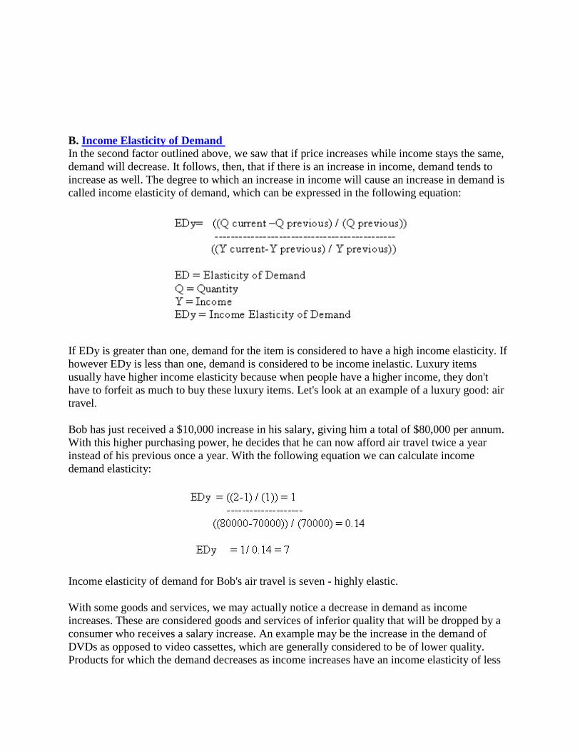
B. Income Elasticity of Demand In the second factor outlined above, we saw that if price increases while income stays the same, demand will decrease. It follows, then, that if there is an increase in income, demand tends to increase as well. The degree to which an increase in income will cause an increase in demand is called income elasticity of demand, which can be expressed in the following equation:

If EDy is greater than one, demand for the item is considered to have a high income elasticity. If however EDy is less than one, demand is considered to be income inelastic. Luxury items usually have higher income elasticity because when people have a higher income, they don't have to forfeit as much to buy these luxury items. Let's look at an example of a luxury good: air travel. Bob has just received a $10,000 increase in his salary, giving him a total of $80,000 per annum. With this higher purchasing power, he decides that he can now afford air travel twice a year instead of his previous once a year. With the following equation we can calculate income demand elasticity:

Income elasticity of demand for Bob's air travel is seven - highly elastic. With some goods and services, we may actually notice a decrease in demand as income increases. These are considered goods and services of inferior quality that will be dropped by a consumer who receives a salary increase. An example may be the increase in the demand of DVDs as opposed to video cassettes, which are generally considered to be of lower quality. Products for which the demand decreases as income increases have an income elasticity of less

than zero. Products that witness no change in demand despite a change in income usually have an income elasticity of zero - these goods and services are considered necessities.

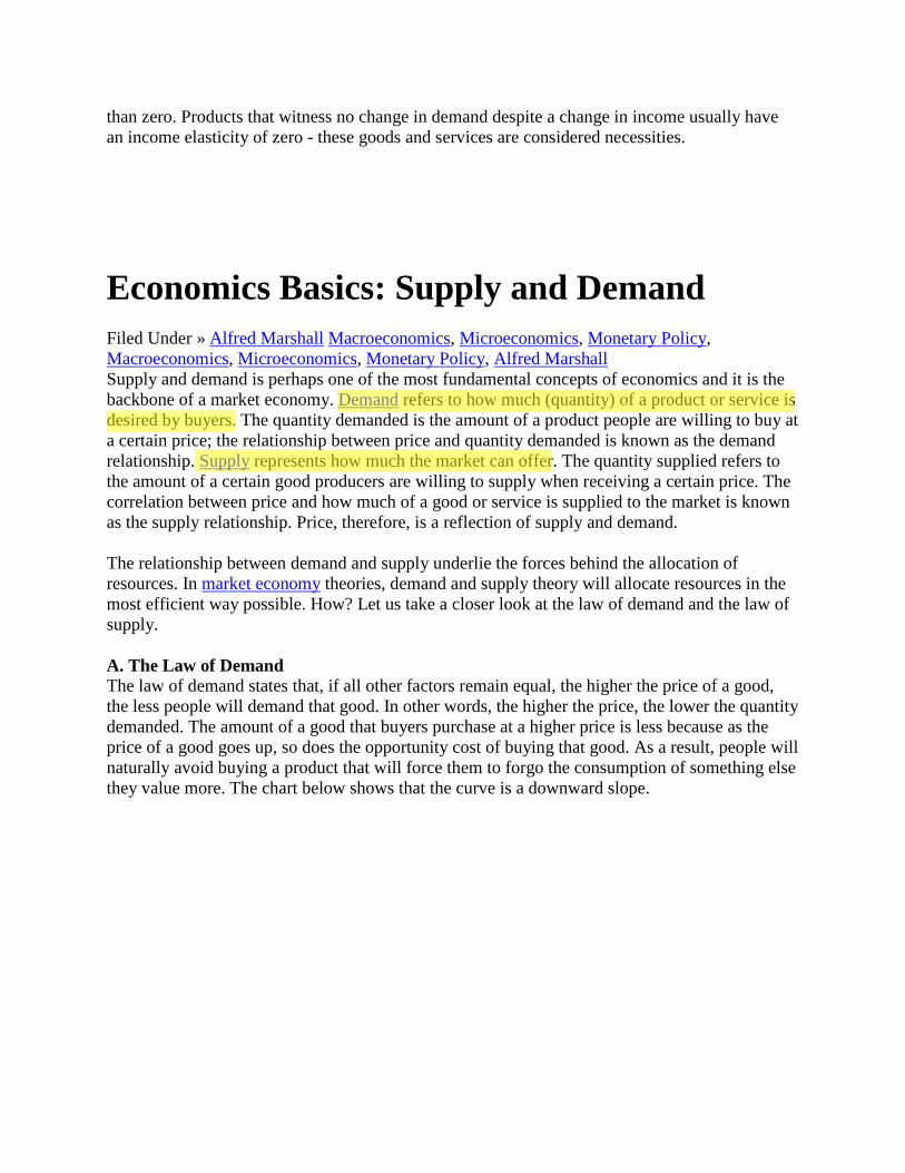
Economics Basics: Supply and Demand Filed Under » Alfred Marshall Macroeconomics, Microeconomics, Monetary Policy, Macroeconomics, Microeconomics, Monetary Policy, Alfred Marshall Supply and demand is perhaps one of the most fundamental concepts of economics and it is the backbone of a market economy. Demand refers to how much (quantity) of a product or service is desired by buyers. The quantity demanded is the amount of a product people are willing to buy at a certain price; the relationship between price and quantity demanded is known as the demand relationship. Supply represents how much the market can offer. The quantity supplied refers to the amount of a certain good producers are willing to supply when receiving a certain price. The correlation between price and how much of a good or service is supplied to the market is known as the supply relationship. Price, therefore, is a reflection of supply and demand. The relationship between demand and supply underlie the forces behind the allocation of resources. In market economy theories, demand and supply theory will allocate resources in the most efficient way possible. How? Let us take a closer look at the law of demand and the law of supply. A. The Law of Demand The law of demand states that, if all other factors remain equal, the higher the price of a good, the less people will demand that good. In other words, the higher the price, the lower the quantity demanded. The amount of a good that buyers purchase at a higher price is less because as the price of a good goes up, so does the opportunity cost of buying that good. As a result, people will naturally avoid buying a product that will force them to forgo the consumption of something else they value more. The chart below shows that the curve is a downward slope.

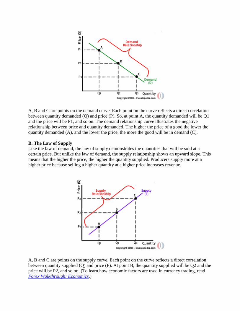
A, B and C are points on the demand curve. Each point on the curve reflects a direct correlation between quantity demanded (Q) and price (P). So, at point A, the quantity demanded will be Q1 and the price will be P1, and so on. The demand relationship curve illustrates the negative relationship between price and quantity demanded. The higher the price of a good the lower the quantity demanded (A), and the lower the price, the more the good will be in demand (C). B. The Law of Supply Like the law of demand, the law of supply demonstrates the quantities that will be sold at a certain price. But unlike the law of demand, the supply relationship shows an upward slope. This means that the higher the price, the higher the quantity supplied. Producers supply more at a higher price because selling a higher quantity at a higher price increases revenue.

A, B and C are points on the supply curve. Each point on the curve reflects a direct correlation between quantity supplied (Q) and price (P). At point B, the quantity supplied will be Q2 and the price will be P2, and so on. (To learn how economic factors are used in currency trading, read Forex Walkthrough: Economics.)

Time and Supply Unlike the demand relationship, however, the supply relationship is a factor of time. Time is important to supply because suppliers must, but cannot always, react quickly to a change in demand or price. So it is important to try and determine whether a price change that is caused by demand will be temporary or permanent. Let's say there's a sudden increase in the demand and price for umbrellas in an unexpected rainy season; suppliers may simply accommodate demand by using their production equipment more intensively. If, however, there is a climate change, and the population will need umbrellas year-round, the change in demand and price will be expected to be long term; suppliers will have to change their equipment and production facilities in order to meet the long-term levels of demand. C. Supply and Demand Relationship Now that we know the laws of supply and demand, let's turn to an example to show how supply and demand affect price. Imagine that a special edition CD of your favorite band is released for $20. Because the record company's previous analysis showed that consumers will not demand CDs at a price higher than $20, only ten CDs were released because the opportunity cost is too high for suppliers to produce more. If, however, the ten CDs are demanded by 20 people, the price will subsequently rise because, according to the demand relationship, as demand increases, so does the price. Consequently, the rise in price should prompt more CDs to be supplied as the supply relationship shows that the higher the price, the higher the quantity supplied. If, however, there are 30 CDs produced and demand is still at 20, the price will not be pushed up because the supply more than accommodates demand. In fact after the 20 consumers have been satisfied with their CD purchases, the price of the leftover CDs may drop as CD producers attempt to sell the remaining ten CDs. The lower price will then make the CD more available to people who had previously decided that the opportunity cost of buying the CD at $20 was too high. D. Equilibrium When supply and demand are equal (i.e. when the supply function and demand function intersect) the economy is said to be at equilibrium. At this point, the allocation of goods is at its most efficient because the amount of goods being supplied is exactly the same as the amount of goods being demanded. Thus, everyone (individuals, firms, or countries) is satisfied with the current economic condition. At the given price, suppliers are selling all the goods that they have produced and consumers are getting all the goods that they are demanding.

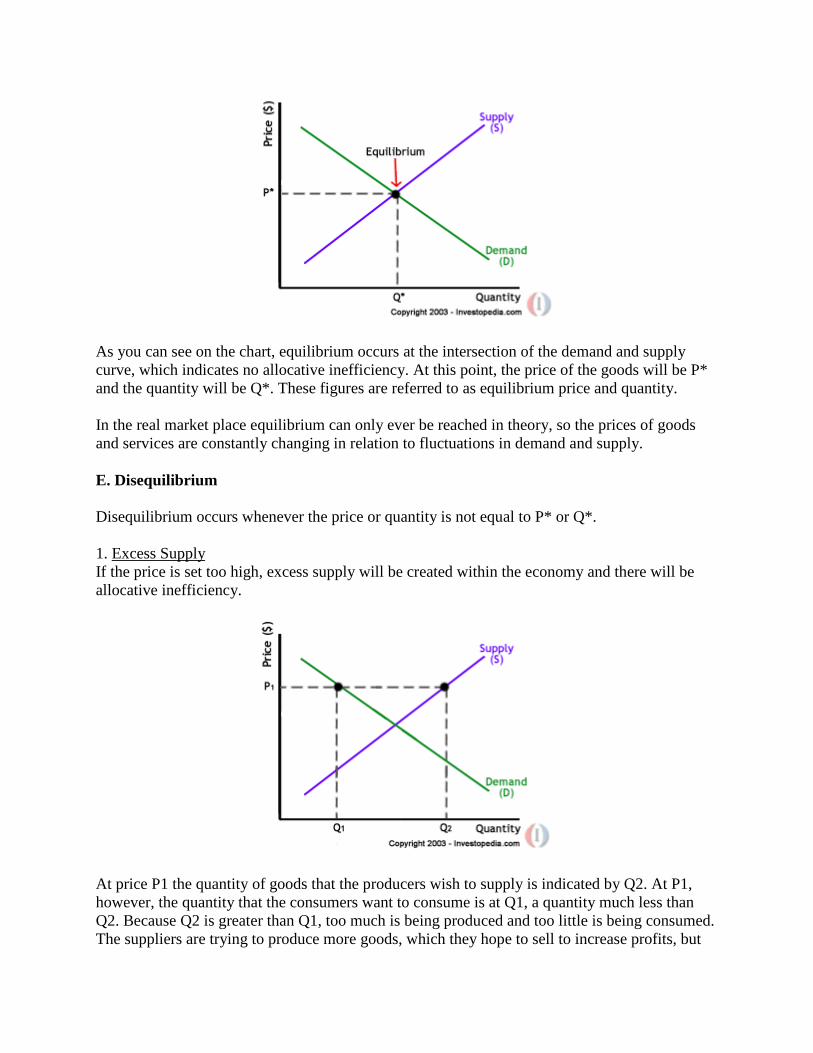
As you can see on the chart, equilibrium occurs at the intersection of the demand and supply curve, which indicates no allocative inefficiency. At this point, the price of the goods will be P* and the quantity will be Q*. These figures are referred to as equilibrium price and quantity. In the real market place equilibrium can only ever be reached in theory, so the prices of goods and services are constantly changing in relation to fluctuations in demand and supply. E. Disequilibrium Disequilibrium occurs whenever the price or quantity is not equal to P* or Q*. 1. Excess Supply If the price is set too high, excess supply will be created within the economy and there will be allocative inefficiency.

At price P1 the quantity of goods that the producers wish to supply is indicated by Q2. At P1, however, the quantity that the consumers want to consume is at Q1, a quantity much less than Q2. Because Q2 is greater than Q1, too much is being produced and too little is being consumed. The suppliers are trying to produce more goods, which they hope to sell to increase profits, but

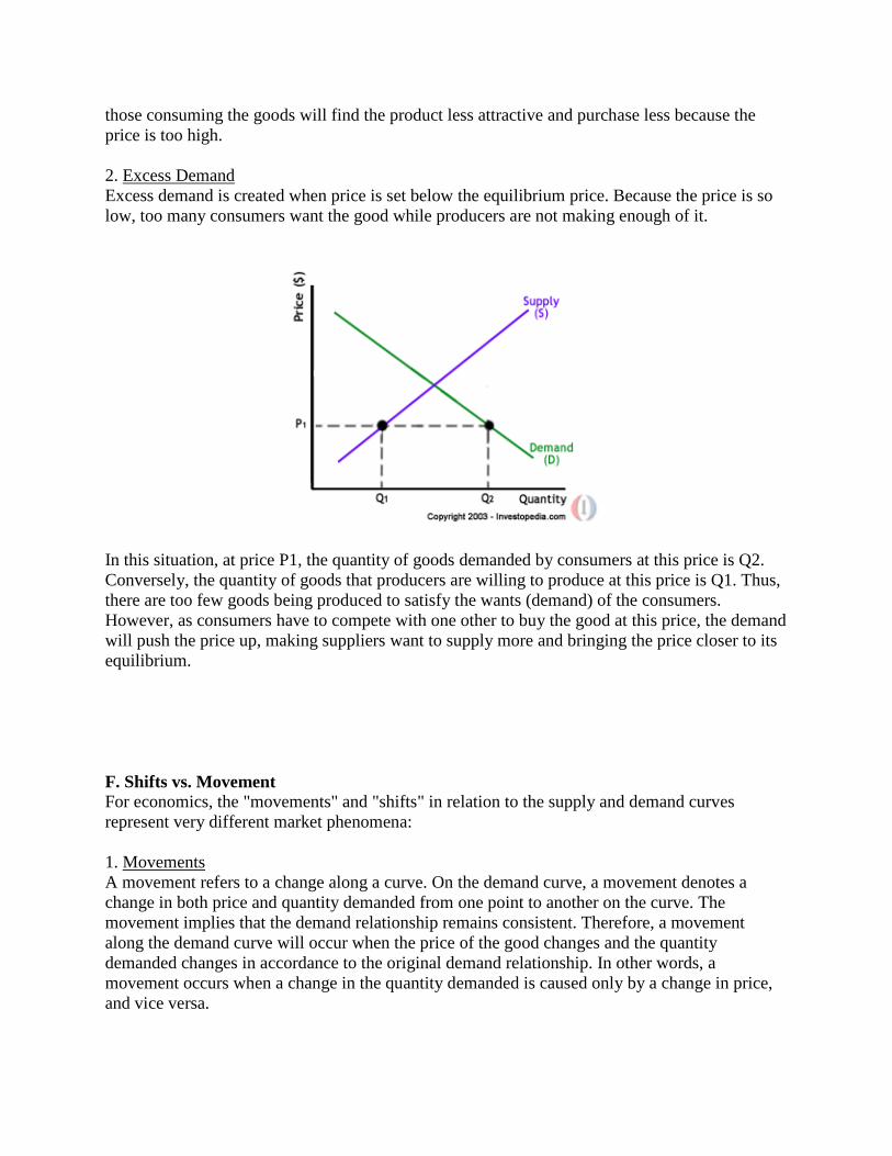
those consuming the goods will find the product less attractive and purchase less because the price is too high. 2. Excess Demand

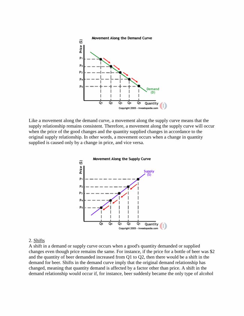
Excess demand is created when price is set below the equilibrium price. Because the price is so low, too many consumers want the good while producers are not making enough of it.

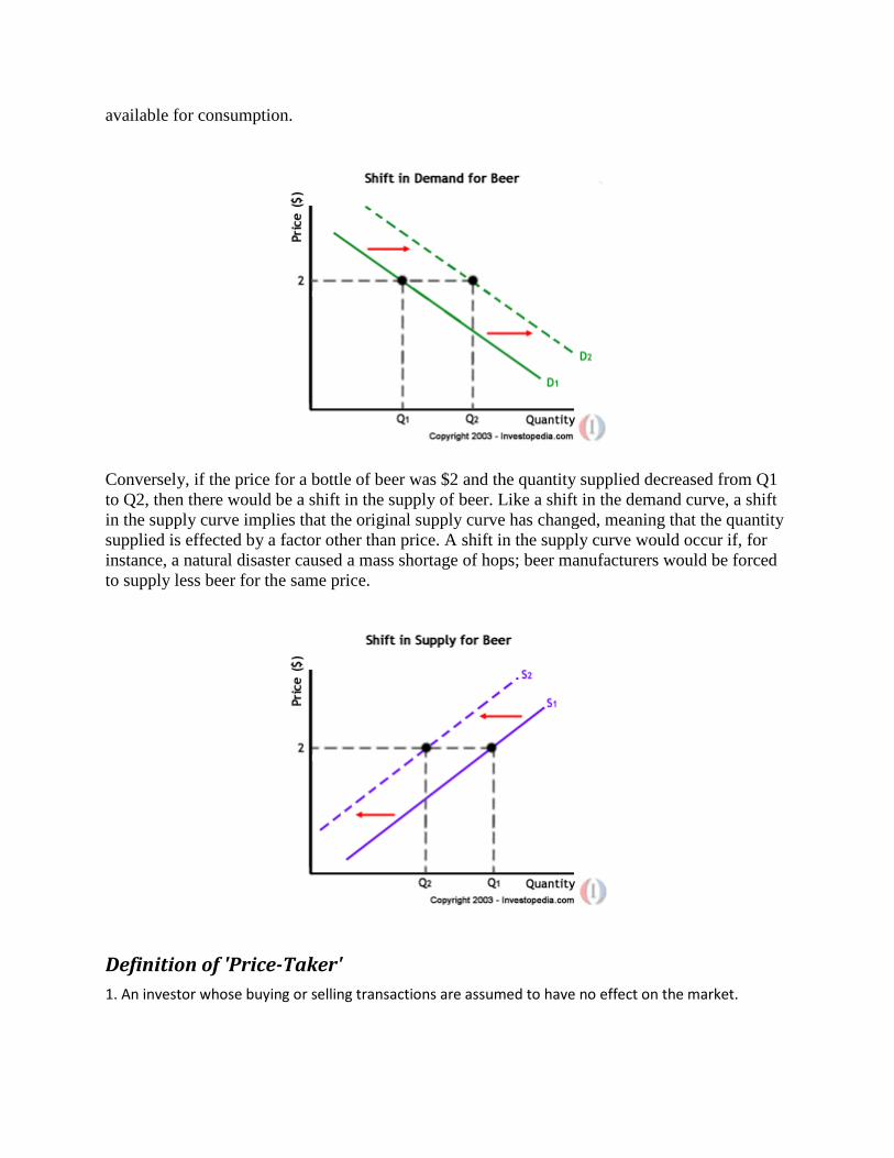
In this situation, at price P1, the quantity of goods demanded by consumers at this price is Q2. Conversely, the quantity of goods that producers are willing to produce at this price is Q1. Thus, there are too few goods being produced to satisfy the wants (demand) of the consumers. However, as consumers have to compete with one other to buy the good at this price, the demand will push the price up, making suppliers want to supply more and bringing the price closer to its equilibrium. F. Shifts vs. Movement For economics, the "movements" and "shifts" in relation to the supply and demand curves represent very different market phenomena: 1. Movements A movement refers to a change along a curve. On the demand curve, a movement denotes a change in both price and quantity demanded from one point to another on the curve. The movement implies that the demand relationship remains consistent. Therefore, a movement along the demand curve will occur when the price of the good changes and the quantity demanded changes in accordance to the original demand relationship. In other words, a movement occurs when a change in the quantity demanded is caused only by a change in price, and vice versa.

Like a movement along the demand curve, a movement along the supply curve means that the supply relationship remains consistent. Therefore, a movement along the supply curve will occur when the price of the good changes and the quantity supplied changes in accordance to the original supply relationship. In other words, a movement occurs when a change in quantity supplied is caused only by a change in price, and vice versa.

2. Shifts A shift in a demand or supply curve occurs when a good's quantity demanded or supplied changes even though price remains the same. For instance, if the price for a bottle of beer was $2 and the quantity of beer demanded increased from Q1 to Q2, then there would be a shift in the demand for beer. Shifts in the demand curve imply that the original demand relationship has changed, meaning that quantity demand is affected by a factor other than price. A shift in the demand relationship would occur if, for instance, beer suddenly became the only type of alcohol

available for consumption.

Conversely, if the price for a bottle of beer was $2 and the quantity supplied decreased from Q1 to Q2, then there would be a shift in the supply of beer. Like a shift in the demand curve, a shift in the supply curve implies that the original supply curve has changed, meaning that the quantity supplied is effected by a factor other than price. A shift in the supply curve would occur if, for instance, a natural disaster caused a mass shortage of hops; beer manufacturers would be forced to supply less beer for the same price.

Definition of 'Price-Taker' 1. An investor whose buying or selling transactions are assumed to have no effect on the market.

2. A firm that can alter its rate of production and sales without significantly affecting the market price of

its product.

Investopedia explains 'Price-Taker' 1. In the context of the stock market, individual investors are price-takers.

2. Suppose you sell water, which of course is supplied by millions of other places, including the sky. If you decide to set the price of a gallon of your water at $10, you will likely sell nothing because this commodity is readily available elsewhere for a much cheaper price.

Definition of 'Price Maker' A monopoly or a firm within monopolistic competition that has the power to influence the price it

charges as the good it produces does not have perfect substitutes.

Investopedia explains 'Price Maker' • A monopoly is a price maker as it holds a large amount of power over the price it charges.

A price maker that is a firm within monopolistic competition produces goods that are differentiated in some way from its competitors' products. This kind of price maker is also a profit-maximizer as it will increase output only as long as its marginal revenue is greater than its marginal cost, in other words, as long as it's producing a profit.

fallacy of composition DefinitionThe

Save to FavoritesSee Examples false assumption that something which is true for one segment of the economy is true for the

economy as a whole. For instance, if one state has an inflated unemployment rate then the whole United States has the same problem.

Production–possibility frontier From Wikipedia, the free encyclopedia Jump to: navigation, search

In economics, a production–possibility frontier ('PPF), sometimes called a production–possibility curve, production-possibility boundary or product transformation curve, is a graph that shows the various combinations of amounts of two commodities that could be produced using the same fixed total amount of each of the factors of production. Graphically bounding the production set for fixed input quantities, the PPF curve shows the maximum possible production level of one commodity for any given production level of the other, given the existing state of technology. By doing so, it defines productive efficiency in the context of that production set: a point on the frontier indicates efficient use of the available inputs, while a point beneath the curve indicates inefficiency. A period of time is specified as well as the production technologies and amounts of inputs available. The commodities compared can either be goods or services.

PPFs are normally drawn as bulging upwards ("concave") from the origin but can also be represented as bulging downward or linear (straight), depending on a number of factors. A PPF can be used to illustrate a number of economic concepts, such as scarcity of resources (i.e., the fundamental economic problem all societies face), opportunity cost (or marginal rate of transformation), productive efficiency, allocative efficiency, and economies of scale. In addition, an outward shift of the PPF results from growth of the availability of inputs such as physical capital or labour, or technological progress in our knowledge of how to transform inputs into outputs. Such a shift allows economic growth of an economy already operating at its full productivity (on the PPF), which means that more of both outputs can be produced during the specified period of time without sacrificing the output of either good. Conversely, the PPF will shift inward if the labor force shrinks, the supply of raw materials is depleted, or a natural disaster decreases the stock of physical capital. However, most economic contractions reflect not that less can be produced, but that the economy has started operating below the frontier—typically both labor and physical capital are underemployed. The combination represented by the point on the PPF where an economy operates shows the priorities or choices of the economy, such as the choice of producing more capital goods and fewer consumer goods or vice versa.

Indicators

Efficiency

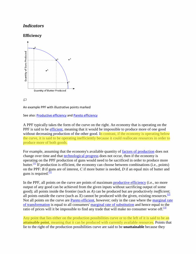
An example PPF with illustrative points marked

See also: Productive efficiency and Pareto efficiency

A PPF typically takes the form of the curve on the right. An economy that is operating on the PPF is said to be efficient, meaning that it would be impossible to produce more of one good without decreasing production of the other good. In contrast, if the economy is operating below the curve, it is said to be operating inefficiently because it could reallocate resources in order to produce more of both goods.

For example, assuming that the economy's available quantity of factors of production does not change over time and that technological progress does not occur, then if the economy is operating on the PPF production of guns would need to be sacrificed in order to produce more butter.[1] If production is efficient, the economy can choose between combinations (i.e., points) on the PPF: B if guns are of interest, C if more butter is needed, D if an equal mix of butter and guns is required.[1]

In the PPF, all points on the curve are points of maximum productive efficiency (i.e., no more output of any good can be achieved from the given inputs without sacrificing output of some good); all points inside the frontier (such as A) can be produced but are productively inefficient; all points outside the curve (such as X) cannot be produced with the given, existing resources.[2] Not all points on the curve are Pareto efficient, however; only in the case where the marginal rate of transformation is equal to all consumers' marginal rate of substitution and hence equal to the ratio of prices will it be impossible to find any trade that will make no consumer worse off.[3]

Any point that lies either on the production possibilities curve or to the left of it is said to be an attainable point, meaning that it can be produced with currently available resources. Points that lie to the right of the production possibilities curve are said to be unattainable because they

cannot be produced using currently available resources. Points that lie within the curve are said to be inefficient, because existing resources would allow for production of more of at least one good without sacrificing the production of any other good. An efficient point is one that lies on the production possibilities curve. At any such point, more of one good can be produced only by producing less of the other. [4]

Such a two-good world is a theoretical simplification, due to the difficulty of graphical analysis of multiple goods. If we are interested in one good, a composite score of the other goods can be generated using different techniques.[5][6] Furthermore, the production model can be generalised using higher-dimensional techniques such as Principal Component Analysis (PCA) and others.[7]

Opportunity cost

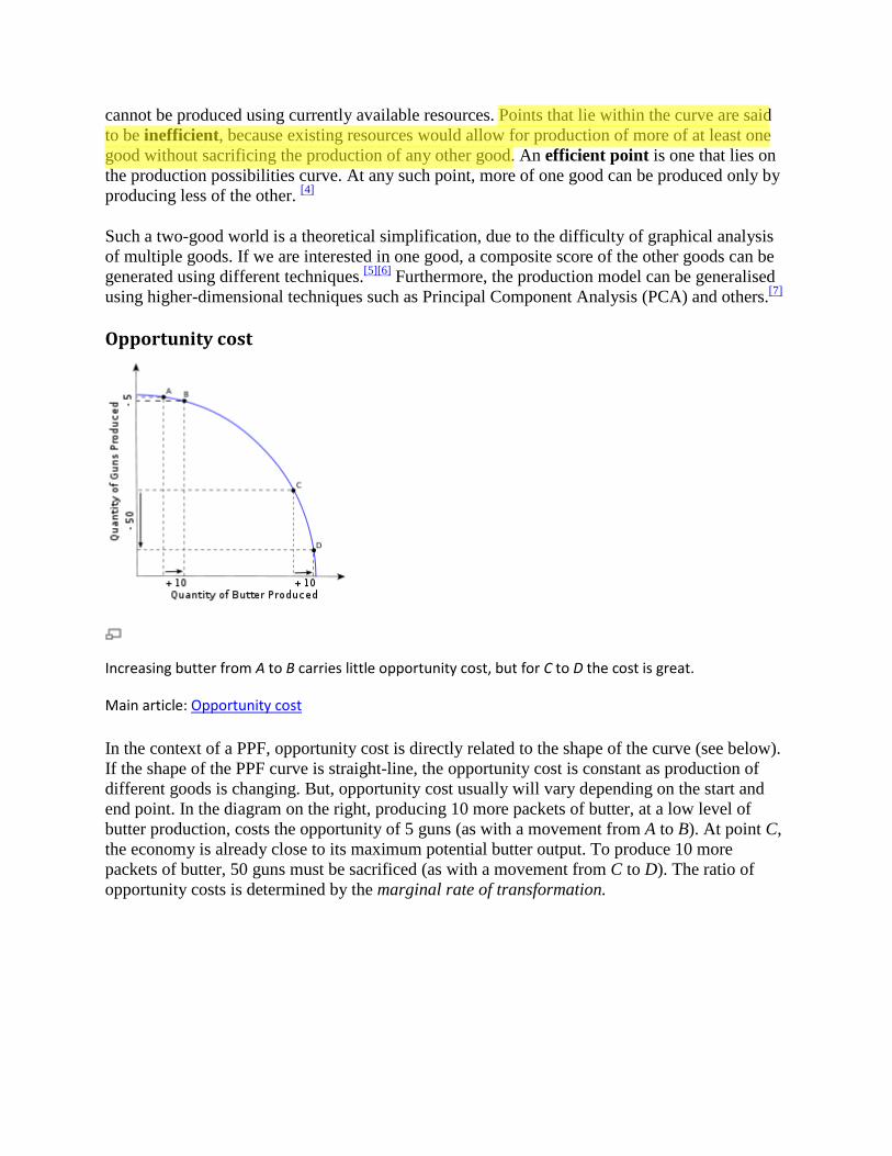
Increasing butter from A to B carries little opportunity cost, but for C to D the cost is great.

Main article: Opportunity cost

In the context of a PPF, opportunity cost is directly related to the shape of the curve (see below). If the shape of the PPF curve is straight-line, the opportunity cost is constant as production of different goods is changing. But, opportunity cost usually will vary depending on the start and end point. In the diagram on the right, producing 10 more packets of butter, at a low level of butter production, costs the opportunity of 5 guns (as with a movement from A to B). At point C, the economy is already close to its maximum potential butter output. To produce 10 more packets of butter, 50 guns must be sacrificed (as with a movement from C to D). The ratio of opportunity costs is determined by the marginal rate of transformation.

Marginal rate of transformation

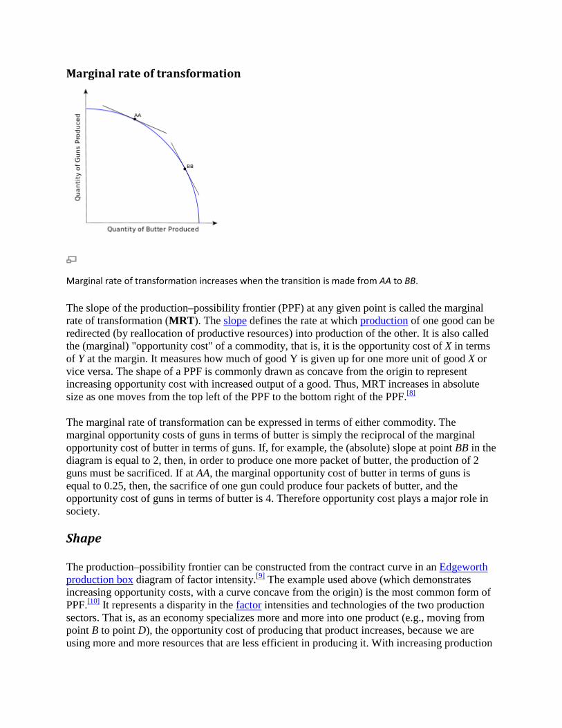
Marginal rate of transformation increases when the transition is made from AA to BB.

The slope of the production–possibility frontier (PPF) at any given point is called the marginal rate of transformation (MRT). The slope defines the rate at which production of one good can be redirected (by reallocation of productive resources) into production of the other. It is also called the (marginal) "opportunity cost" of a commodity, that is, it is the opportunity cost of X in terms of Y at the margin. It measures how much of good Y is given up for one more unit of good X or vice versa. The shape of a PPF is commonly drawn as concave from the origin to represent increasing opportunity cost with increased output of a good. Thus, MRT increases in absolute size as one moves from the top left of the PPF to the bottom right of the PPF.[8]

The marginal rate of transformation can be expressed in terms of either commodity. The marginal opportunity costs of guns in terms of butter is simply the reciprocal of the marginal opportunity cost of butter in terms of guns. If, for example, the (absolute) slope at point BB in the diagram is equal to 2, then, in order to produce one more packet of butter, the production of 2 guns must be sacrificed. If at AA, the marginal opportunity cost of butter in terms of guns is equal to 0.25, then, the sacrifice of one gun could produce four packets of butter, and the opportunity cost of guns in terms of butter is 4. Therefore opportunity cost plays a major role in society.

The production–possibility frontier can be constructed from the contract curve in an

Shape

Edgeworth production box diagram of factor intensity.[9] The example used above (which demonstrates increasing opportunity costs, with a curve concave from the origin) is the most common form of PPF.[10] It represents a disparity in the factor intensities and technologies of the two production sectors. That is, as an economy specializes more and more into one product (e.g., moving from point B to point D), the opportunity cost of producing that product increases, because we are using more and more resources that are less efficient in producing it. With increasing production

of butter, workers from the gun industry will move to it. At first, the least qualified (or most general) gun workers will be transferred into making more butter, and moving these workers has little impact on the opportunity cost of increasing butter production: the loss in gun production will be small. But the cost of producing successive units of butter will increase as resources that are more and more specialized in gun production are moved into the butter industry.[11]

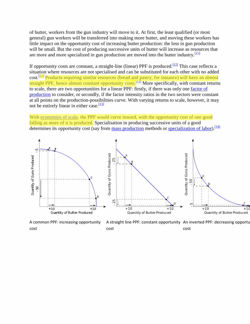
If opportunity costs are constant, a straight-line (linear) PPF is produced.[12] This case reflects a situation where resources are not specialised and can be substituted for each other with no added cost.[11] Products requiring similar resources (bread and pastry, for instance) will have an almost straight PPF, hence almost constant opportunity costs.[11] More specifically, with constant returns to scale, there are two opportunities for a linear PPF: firstly, if there was only one factor of production to consider, or secondly, if the factor intensity ratios in the two sectors were constant at all points on the production-possibilities curve. With varying returns to scale, however, it may not be entirely linear in either case.[13]

With economies of scale, the PPF would curve inward, with the opportunity cost of one good falling as more of it is produced. Specialisation in producing successive units of a good determines its opportunity cost (say from mass production methods or specialization of labor).[14]

A common PPF: increasing opportunity cost

A straight line PPF: constant opportunity cost

An inverted PPF: decreasing opportunity cost

Position

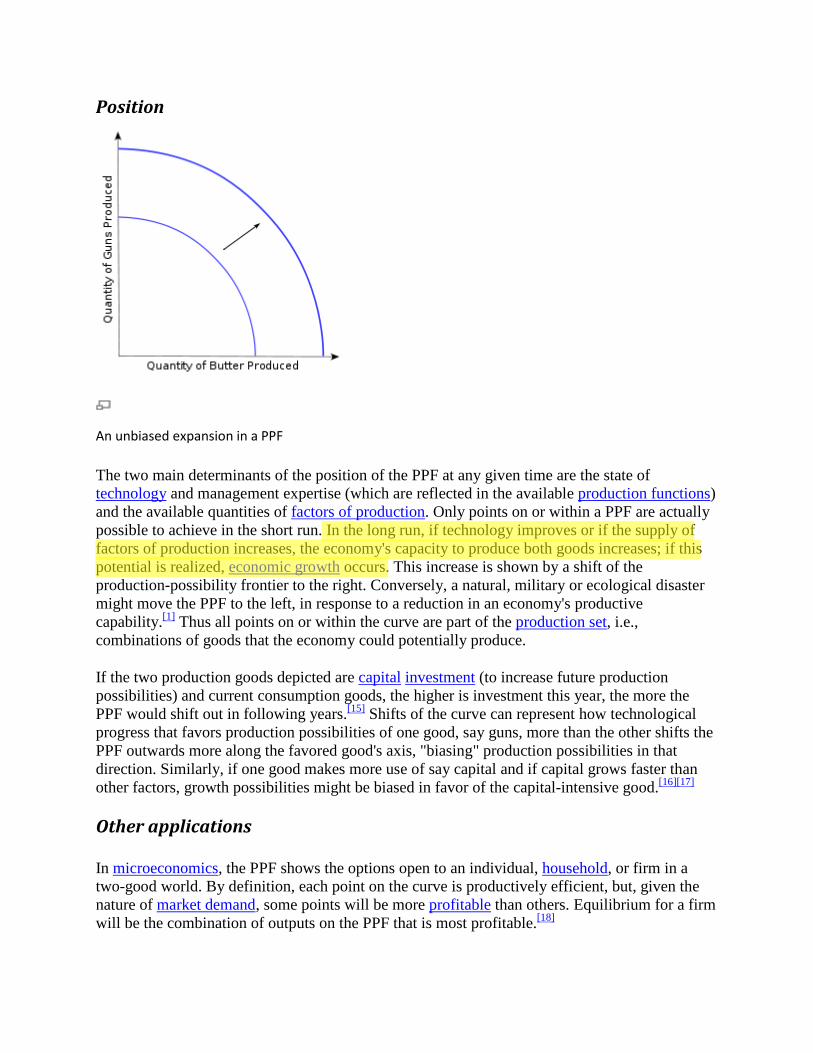
An unbiased expansion in a PPF

The two main determinants of the position of the PPF at any given time are the state of technology and management expertise (which are reflected in the available production functions) and the available quantities of factors of production. Only points on or within a PPF are actually possible to achieve in the short run. In the long run, if technology improves or if the supply of factors of production increases, the economy's capacity to produce both goods increases; if this potential is realized, economic growth occurs. This increase is shown by a shift of the production-possibility frontier to the right. Conversely, a natural, military or ecological disaster might move the PPF to the left, in response to a reduction in an economy's productive capability.[1] Thus all points on or within the curve are part of the production set, i.e., combinations of goods that the economy could potentially produce.

If the two production goods depicted are capital investment (to increase future production possibilities) and current consumption goods, the higher is investment this year, the more the PPF would shift out in following years.[15] Shifts of the curve can represent how technological progress that favors production possibilities of one good, say guns, more than the other shifts the PPF outwards more along the favored good's axis, "biasing" production possibilities in that direction. Similarly, if one good makes more use of say capital and if capital grows faster than other factors, growth possibilities might be biased in favor of the capital-intensive good.[16][17]

In

Other applications

microeconomics, the PPF shows the options open to an individual, household, or firm in a two-good world. By definition, each point on the curve is productively efficient, but, given the nature of market demand, some points will be more profitable than others. Equilibrium for a firm will be the combination of outputs on the PPF that is most profitable.[18]

From a macroeconomic perspective, the PPF illustrates the production possibilities available to a nation or economy during a given period of time for broad categories of output. It is traditionally used to show the movement between committing all funds to consumption on the y-axis versus investment on the x-axis. However, an economy may achieve productive efficiency without necessarily being allocatively efficient. Market failure (such as imperfect competition or externalities) and some institutions of social decision-making (such as government and tradition) may lead to the wrong combination of goods being produced (hence the wrong mix of resources being allocated between producing the two goods) compared to what consumers would prefer, given what is feasible on the PPF.[19]

Definition of 'Gross Domestic Product - GDP' The monetary value of all the finished goods and services produced within a country's borders in a specific time period, though GDP is usually calculated on an annual basis. It includes all of private and public consumption, government outlays, investments and exports less imports that occur within a defined territory. GDP = C + G + I + NX where: "C" is equal to all private consumption, or consumer spending, in a nation's economy "G" is the sum of government spending "I" is the sum of all the country's businesses spending on capital "NX" is the nation's total net exports, calculated as total exports minus total imports. (NX = Exports -

Imports)

Investopedia explains 'Gross Domestic Product - GDP' GDP is commonly used as an indicator of the economic health of a country, as well as to gauge a country's standard of living. Critics of using GDP as an economic measure say the statistic does not take into account the underground economy - transactions that, for whatever reason, are not reported to the government. Others say that GDP is not intended to gauge material well-being, but serves as a measure of a nation's productivity, which is unrelated.

Definition of 'Marginal Propensity To Consume - MPC' A component of Keynesian theory, MPC represents the proportion of an aggregate raise in pay that is

spent on the consumption of goods and services, as opposed to being saved.

Investopedia explains 'Marginal Propensity To Consume - MPC' Let's illustrate this with an example. Suppose you receive a bonus with your paycheck, and it's $500 on top of your normal annual earnings. You suddenly have $500 more in income than you did before. If you decide to spend $400 of this marginal increase in income on a new business suit, your marginal propensity to consume will be 0.8 ($400 divided by $500).