Micro-finance and Poverty:

Evidence Using Panel Data from Bangladesh

Shahidur R. Khandker*

The World Bank

Abstract Micro-finance supports mainly informal activities that often have low market demand. It may be thus hypothesized that the aggregate poverty impact of micro-finance in an economy with low economic growth is modest or non-existent. The observed borrower-level poverty impact is then a result of income redistribution or short-run income generation. The paper addresses these questions using household level panel data from Bangladesh. The findings confirm that micro-finance benefits the poorest, and has sustained impact on poverty reduction among program participants. It has also positive spillover impact, reducing poverty at the village level. But the effect is more pronounced in reducing extreme than moderate poverty. World Bank Policy Research Working Paper 2945, January 2003 The Policy Research Working Paper Series disseminates the findings of work in progress to encourage the exchange of ideas about development issues. An objective of the series is to get the findings out quickly, even if the presentations are less than fully polished. The papers carry the names of the authors and should be cited accordingly. The findings, interpretations, and conclusions expressed in this paper are entirely those of the authors. They do not necessarily represent the view of the World Bank, its Executive Directors, or the countries they represent. Policy Research Working Papers are available online at http://econ.worldbank.org. *I have benefited from discussions with Mark Pitt, Martin Ravallion, Gershon Feder, Binayak Sen, and M. A. Latif and also comments from the participants of a workshop in Manila organized by the Asian Development Bank. I am grateful to Hussain Samad for excellent research assistance and the BIDS project staff for help in the data collection and processing.

1

Micro-finance and Poverty:

Evidence Using Panel Data from Bangladesh

I. Introduction

The objective of this paper is to estimate the long-run impacts of micro-finance on household

consumption and poverty in Bangladesh, based on household survey data collected in 1991/92 and

1998/99. Since its advent in early 1980s micro-finance has been the focus of many development

issues. Bangladesh is the pioneer of the micro-finance movement and the home of the largest

micro-finance operation in the world.. Development practitioners have been keen to know the

extent of poverty reduction possible with micro-finance operation that mostly supports the poor.

Micro-finance means small-scale transactions of credit and savings. As such, it is largely meant to

meet the needs of small- and medium-scale producers and businesses. The poor, especially

women, are the target of micro-finance organizations in many countries, including Bangladesh.

Besides financial services, micro-finance sometimes offers skill-based training to augment

productivity or organizational support and consciousness-raising training to empower the poor.

How much poverty reduction is possible with micro-finance? Benefiting from a micro-

finance program, unlike other transfer schemes, requires not only an individual’s own

entrepreneurship but also a favorable local market. Even if the marginal gains from micro-

borrowing accrued to participants may be large, the accrued total benefits from micro-finance in

reducing poverty are likely to be small, as micro-finance transactions are often too small in

volume to have a sustained aggregate impact on poverty reduction. In an economy where there is

not much growth, borrowing by the poor can improve income redistribution. Thus, it is of policy

interest to know whether accrued benefits at the borrower level are due to sustained income impact

or simple income redistribution. This involves an assessment of long-term poverty impacts of

micro-finance.

2

This paper uses household panel data from Bangladesh to address three issues. First, it

will determine whether the poor who lack both physical (such as land) and human capital (such as

education) actually participate more in micro-finance programs. Second, the paper will assess the

long-term impacts of micro-finance on poverty. Third, it will assess the aggregate impact of

micro-finance to determine if the program is helping the poor beyond program participation.

The paper is organized as follows. Section two reviews current literature on the micro-

finance programs in Bangladesh. Section three outlines the research framework, while section

four discusses the data to be used in the impact analysis of micro-finance programs. Section five

presents estimates of who participates in micro-finance programs in Bangladesh. Section six

reports the impact estimates at the borrower level. Section seven discusses the spillover impacts

of micro-finance. Finally, the results are summarized in the concluding section.

II. What we already know about micro-finance in Bangladesh

Unlike their formal counterpart, micro-finance organizations in Bangladesh have made their stride

in delivering financial services (both savings and credit) to the poor, especially women, at a very

low loan default cost. Strategies such as collateral-free group-based lending and mobilization of

savings, even in small amounts, have helped them mitigate the problems of poor outreach and high

loan default costs of their formal counterpart. However, they assume high transaction costs in

order to keep credit discipline among borrowers through group pressure and monitoring of

borrowers’ behavior. The transaction cost is substantial and programs have been relying on

donors for sustaining their operations (e.g., Khandker 1998; Khalily, Imam, and Khan, 2000;

Morduch 1999; Yaron 1994). Nonetheless, the government and donors continue to support micro-

finance programs in Bangladesh with the expectation that society benefits from such investment.

Micro-finance programs support the production and consumption of the poor. Loans in

easy repayment terms help smooth consumption and create jobs for the unemployed. Resources

from donors have alternative uses such as building community infrastructure, school or health

facilities. Thus, there are many ways by which the poor can benefit from the resources used in

micro-finance programs. For government and donors, the issue is clear: if it is evident that micro-

3

finance programs do not benefit the poor in a sustainable way, then the resources channeled to

micro-finance are misplaced.

Therefore, policymakers and program organizers are keen to learn the extent of

socioeconomic impacts of micro-finance on borrowers and on society at large. At the household

level, two types of impacts can be carried out―household and individual impacts of micro-

finance. Household level impacts such as impacts on income, employment, and poverty are

assessments without specifying the intra-household distribution of induced benefits of micro-

finance. Intra-household impacts are examined to learn the distribution of benefits among

different members of households, especially between men and women. Since women are

disadvantaged in a society such as Bangladesh and constitute the overwhelming share of micro-

finance membership, the policy question is: do women benefit from micro-finance and if so, how?

At the societal level, the policy question is: do micro-finance programs benefit non-program

participants or do they simply help redistribute income in a society?

While the financial review of micro-finance programs in Bangladesh is not as promising as

one would expect, the literature on the impact assessment of socioeconomic benefits of micro-

finance programs shows micro-finance as a promising instrument for poverty reduction.

Findings, of course, differ from one study to another because of the differences in impact

assessment methodologies used; however, these studies are in agreement that micro-finance

programs help the poor, although all participants may not benefit equally. One of the early

studies of Grameen Bank shows how Grameen Bank has been supporting the poor, especially

women, in terms of employment, income generation and promotion of social indicators (Hossain

1988). Other BIDS (Bangladesh Institute of Development Studies) and non-BIDS studies also

indicate the beneficial aspects of micro-finance operation in Bangladesh (e.g., Rahman 1996;

Hashemi, Schuler, and Riley 1996; Schuler and Hashemi 1994). These studies show the positive

correlation between micro-finance programs and their accrued benefits, but do not indicate the

causality, meaning whether these programs actually matter in generating such benefits to the

borrowers.

4

The most comprehensive and rigorous micro-finance impacts studies that have established

causality were carried out in a joint research by BIDS and the World Bank (Khandker 1998; Pitt

and Khandker 1998). This body of research provides a strong indication that the programs help the

poor in consumption smoothing as well as in building assets. The findings also lend support to the

claim that micro-finance programs promote investment in human capital (such as schooling) and

contribute to increasing awareness to reproductive health (such as the use of contraceptives)

among poor families. This major study also sheds lights on the role of gender-based targeting and

its impact on household or individual welfare. Findings suggest that women do acquire assets of

their own and exercise power in household decision-making.1

The positive impacts of micro-finance programs at the borrower level are thus tenable.

Even then, the question arises: what are the long-run impacts of micro-finance? Are the program

impacts found in 1991/92 sustainable over time? If poverty reduction is possible with micro-

finance at the borrower level, what is the impact of micro-finance on aggregate poverty? Earlier

estimates suggest that micro-finance can contribute to consumption at a rate of 18 percent in the

case of female borrowing and at 11 percent in the case of male borrowing. Of course, this is a

short-term impact and, hence, may be short-lived. It is possible that the proportion of program

participants enjoying the benefits of micro-finance is very small and that the impacts of their

accrued benefits on the overall economy are small as well and may not be sustainable over time.

The World Bank study based on the 1991/92 household survey indicates that only about

less than 5 percent of borrowers can lift themselves out of poverty each year by borrowing from a

micro-finance program even if the estimated impacts on consumption are sustained over time

(Khandker 1998). Such percentage represents only about 1 percent of the population; thus, the

aggregate poverty impact of micro-finance program is quite negligible. Does it imply that micro-

finance programs do not need to be supported?

1 Morduch (1998), using the same BIDS-World Bank survey data but a different technique (difference-in-difference method), finds that program effects are either non-existent or very small. He argues that the Pitt and Khandker (1998) estimates of program impacts are over-estimated and, thus, the flagship programs such as the Grameen Bank do not really help the poor. Pitt (1999) re-examined Morduch’s (1999) approach and concluded that Morduch applied a wrong method to the BIDS-World Bank data set, which in fact underestimated the program impacts. Pitt’s re-estimation re-confirms that the impacts of Grameen Bank and other programs as shown in the Pitt and Khandker (1998) study are indeed well founded. For those who are interested in Pitt’s analysis of Morduch’s re-analysis of Pitt and Khandker (1998), go to http://pstc3.pstc.brown.edu/~mp/

5

Despite this miniscule aggregate impact, the micro-finance movement in Bangladesh has

received continuous support from donors, and more recently from the World Bank. In 1996, the

World Bank provided a loan of US$115 million to the country’s autonomous body called Palli

Karma Shahayak Foundation (PKSF). This body works as an intermediary for wholesaling micro-

finance. It supports the on-lending of small non-government organizations (NGOs) and a few

large NGOs such as the Bangladesh Rural Advancement Committee (BRAC). However, the

Grameen Bank did not seek any loan or grant from this facility. The project ended in June 2000

and the World Bank, with the request from the government, supported a follow-up project of US$

160 million. With the flow of funds from various micro-finance agencies to borrowers, about 8

million (out of a total of approximately 30 million) households received help from micro-finance

programs in 1998/99.2 Loan outstanding of micro-finance programs was about US$600 million in

1998/99. The organized NGO sector and the specialized Grameen Bank accounted for more than

86 percent of micro-finance lending, while only 14 percent came from the country’s commercial

banks.3

Despite the large inflow of micro-credit into the rural sector of Bangladesh, the incidence

of rural poverty has been stubbornly high. Rural poverty was 54 percent in 1983/84 and has been

above 50 percent over the last decade (Ravallion and Sen 1995). It has declined to about 45

percent in recent years; yet the incidence of poverty has remained high. Critics argue that this

reflects the limitation of micro-finance programs as an instrument in arresting poverty in a

country, which has the largest micro-finance operation in the world. Is the high incidence of

poverty a result of the failure of micro-finance movement? Or is it an outcome of the persistently

low economic growth rate (which has been only 4 percent over the last decade) in the country? If

substantial poverty reduction largely depends on sustained high economic growth, what is the net

overall contribution of the micro-finance movement in Bangladesh?

2 This means about a quarter of rural households were direct beneficiaries of microfinance in Bangladesh in 1998/99. 3 There is a common misconception among many people that Grameen Bank is an NGO. On the contrary, it is a specialized bank with its own charter approved by the government of Bangladesh.

6

III. Impact assessment using panel data

The sources of bias in any program impact assessment are the non-randomness of program

placement and program participation. In many cases, antipoverty programs, such as the Grameen

Bank, are placed in areas with high incidence of poverty. Thus, by comparing the incidence of

poverty in program and non-program areas, researchers may mistakenly conclude that micro-credit

programs have increased poverty. Similarly, those who participate actually may self-select into a

program based on unobserved traits such as entrepreneurial ability. Thus, by comparing behavioral

outcomes, such as per capita consumption of food and non-food, between participants and non-

participants, evaluators may mistakenly conclude that the program has a high impact on poverty

even if part of the effects is due to the unobserved ability of the participants and has nothing to do

with the program. In other words, it is possible that the estimated program effects may well be

under- or overestimated depending on the circumstances.

A careful study clearly shows that endogeneity of both micro-credit program placement

and program participation is a serious issue and the findings could be misleading if the

endogeneity is not taken into account in the estimation (Pitt and Khandker 1998). The method

used by Pitt and Khandker (1998) is based on cross-section data but they employed a quasi-

experimental survey design to resolve the problems of endogeneity associated with non-random

program placement and self-selected program participation.

Three components of the quasi-experimental survey design are: (a) households are sampled

in villages that are with and without programs; (b) both eligible and ineligible households are

sampled in both types of villages; and (c) program participants and non-participants within eligible

households are sampled. The two central underlying conditions for program impact identification

are: (i) exogenous landholding and (ii) gender-based program design. Since only the households

with landholding of less than half of an acre are eligible, this helps to identify the program impact

on participants by distinguishing who participates and who does not even if both are eligible to

join a micro-credit program. However, program effects are conditioned by why certain villages

are treated with a program by drawing randomly both program villages and non-program villages.

The villages are further identified by women-only and men-only groups, which in turn helped

identify program impacts by gender of program participants.

7

The quasi-experimental survey design is one of many methods evaluators use to assess

program effects. There are three compelling reasons for an impact analysis using a panel survey

over a cross-sectional survey: (i) Cross-section results may not be robust as some studies show

that measurement of program impacts depends importantly on the methods used to treat program

endogeneity (e.g., Lalonde 1986). (ii) It is important to see the robustness of the results with a

method other than the one used in Pitt and Khandker (1998). With panel data, the household-level

fixed-effects method is less reliant on the exact application of the landholding rule by the micro-

credit programs. (iii) Cross-section data provide short-term program effects; however, program

takes a long time to influence outcomes such as assets or human capital investment in children.

Panel data analysis will help measure the program effects on long-term household or individual

welfare .

To show how the panel data can be used to estimate program effects, assume the following

reduced-form borrowing by women (Bijf) and men (Bijm) of i-th households in j-th village in period

t:

bijft

bjf

bijfbfijtijft XB εµηβ +++= (1)

bijmt

bjm

bijmbmijtijmt XB εµηβ +++= (2)

where X is a vector of household characteristics (e.g., age and education of household head), β is a

vector of unknown parameters to be estimated, η is an unmeasured determinant of the credit

demand that is time-invariant and fixed within a household, µ is an unmeasured determinant of the

credit demand that is time-invariant and fixed within a village, and ε is a non-systematic error.

The conditional demand for consumption (Cijt) in each period conditional on the level of

borrowing by male (Bijmt) and that by female (Bijft) for each period, is given as4

4 The justification for including borrowing into the dynamic consumption equation such as (3) can be done by modifying the Ramsey consumption growth model by allowing marginal product of capital to depend on the level of borrowing in the presence of constraints on capital mobility, making households credit constrained (a similar argument on geographical capital immobility has been mentioned as a factor in consumption growth in Jalan and Ravallion 2002). Assuming that households are credit constrained, the marginal product of capital depends on borrowing (B), given by r(B). An optimization of consumption over time subject to production constraints can lead to

8

cijt

cij

cijmijmtfijftcijtijt BBXC εµηδδβ +++++= (3)

where δf and δm are the effects of female and male credit, respectively.

The impact of credit on household outcomes such as consumption can be measured by

estimating equation (3). However, the credit demand by either male or female as given in

equations (1) and (2) needs to be estimated jointly with equation (3). Using cross-section data

(t=1) raises endogeneity of equation (3) on equations (1) and (2) as a result of the possible

correlation among errors between borrowing equations and errors among borrowing and

consumption equations (Pitt and Khandker 1998). However, equation (3) includes no variables

that are not included in equations (1) and (2) or vice versa. That means, the estimating equation

(3) is not distinguishable from equations (1) and (2).

Pitt and Khandker (1998) used a village-level fixed-effect method to resolve program

placement (or village-level) endogeneity of the 1991/92 data. But they could not use fixed-effect

method at the household level to resolve endogeneity of household participation because of the

non-availability of a household panel (t=1). So they adopted a two-stage instrumental variable

(IV) method to resolve the endogeneity of a household’s participation. In the IV method, they used

exogenous gender- and landholding-based exclusion restrictions to create discontinuous

household’s program choice variable. That variable was interacted with household’s observable

characteristics to create instruments.

With panel data where households have more than one observation (t>1), such two-stage

identification restrictions are not required. This is simply done by differencing out the unobserved

village and household attributes, which are the sources of correlation between the credit demand

and household outcome equations. Differencing equation (3) at two points of time yields the

following outcome equation

an optimal rate of consumption growth C(t) as a function of the rate of return to capital (which is constrained by borrowing), rate of depreciation, and subjective rate of time reference. Assume that the error terms include these subjective rate of time preference and rate of depreciation.

9

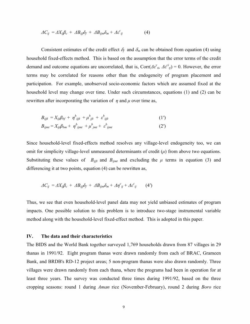
∆Cij = ∆Xijβc + ∆Bijfδf + ∆Bijmδm + ∆εcij (4)

Consistent estimates of the credit effect δf and δm can be obtained from equation (4) using

household fixed-effects method. This is based on the assumption that the error terms of the credit

demand and outcome equations are uncorrelated, that is, Corr(∆εyti, ∆εci

tj) = 0. However, the error

terms may be correlated for reasons other than the endogeneity of program placement and

participation. For example, unobserved socio-economic factors which are assumed fixed at the

household level may change over time. Under such circumstances, equations (1) and (2) can be

rewritten after incorporating the variation of η and µ over time as,

Bijft = Xijtβbf + ηbijft + µb

jft + εbijft (1′)

Bijmt = Xijtβbm + ηbijmt + µb

jmt + εbijmt (2′)

Since household-level fixed-effects method resolves any village-level endogeneity too, we can

omit for simplicity village-level unmeasured determinants of credit (µ) from above two equations.

Substituting these values of Bijft and Bijmt and excluding the µ terms in equation (3) and

differencing it at two points, equation (4) can be rewritten as,

∆Cij = ∆Xijβc + ∆Bijfδf + ∆Bijmδm + ∆ηcij + ∆εc

ij (4′)

Thus, we see that even household-level panel data may not yield unbiased estimates of program

impacts. One possible solution to this problem is to introduce two-stage instrumental variable

method along with the household-level fixed-effect method. This is adopted in this paper.

IV. The data and their characteristics

The BIDS and the World Bank together surveyed 1,769 households drawn from 87 villages in 29

thanas in 1991/92. Eight program thanas were drawn randomly from each of BRAC, Grameen

Bank, and BRDB's RD-12 project areas; 5 non-program thanas were also drawn randomly. Three

villages were drawn randomly from each thana, where the programs had been in operation for at

least three years. The survey was conducted three times during 1991/92, based on the three

cropping seasons: round 1 during Aman rice (November-February), round 2 during Boro rice

10

(March-June), and round 3 during Aus rice (July-October). However, because of attrition, only

1,769 households were available in the third round.

Out of 1,769 households surveyed in 1991/92 by program participation status, 8.5 percent

were Grameen Bank members, 11.6 percent were BRAC members, 6.2 percent were RD-12

project members, 40.3 percent were eligible non-participants, and 33.1 percent were non-target

households (Table 1). A follow-up survey of the same households was done in 1998/99. During

the re-survey, new households from the old villages and new villages in old thanas, and from three

new thanas were included, thereby augmenting the sample households to 2,599.5 According to the

re-survey, 14.3 percent households were Grameen Bank members; 9.3 percent BRAC members;

3.6 percent RD-12 project members; 11.1 percent other NGO members; 7.4 percent multiple

program members; 25.6 percent eligible non-participants; and 28.8 percent non-target households.

Comparing the two surveys, the extent of program participation among rural households has

increased from 26.3 percent in 1991/92 to 45.6 percent in 1998/99.

If participation is restricted to eligible households, the extent of program participation

increased to 64.2 percent in 1998/99 from 39.5 percent in 1991/92. The annual dropout rate,

which was about 5.5 percent in 1991/92, increased to about 29.3 percent in 1998/99. Net program

participation among the eligible households, after adjusting for the dropouts, was 37.1 percent in

1991/92 and 45.3 percent in 1998/99. Even after adjustments due to attrition, the program

participation has increased over the years. This suggests that programs must have benefited

participants; otherwise, the extent of program participation among the eligible households would

not have increased.

Program participation among landless and land-poor households is higher than that among

landed households. For example, the participation rate is 56 percent in 1991/92 and 59 percent in

1998/99 among the landless households (Table 2). Among those who hold land up to 50 decimals

(first three groups in the table), the participation rate increased from 33.9 percent in 1991/92 to

5 Among the 1,769 households surveyed in 1991/92 survey, 131 could not be re-traced in 1998/99 because of attrition, leaving 1,638 households available for the re-survey. However because of household split-offs, 237 original households split to form 546 households in 1998/99, resulting in 1,947 household counts from original survey. Added to them were 652 new households from 1998/99 survey, making total households to 2,599. Khandker and Pitt (2002), in a separate paper, addressed the issue of bias due to attrition and split-offs in the same survey.

11

56.1 percent in 1998/99. Not all households among program participants, however, strictly meet

the land-based eligibility criteria of micro-finance programs. The extent of potential mistargeting

has not changed much since 1991/92. About 23 percent of program borrowers came from non-

target households (those having 50+ decimals of land) in 1991/92 compared to 25 percent in

1998/99 (Table 2). Among the participants, the ultra poor (households owning less than or equal

to 20 decimals of land) constitute about 33 percent in the 1991/92 survey and 58 percent in the

1998/99 survey.6

The extent of multiple membership is a new phenomenon that surfaced in the re-survey.

Cases of households being members of more than one program at the same time have been

reported in the 1998/99 survey but not in the 1991/92 survey. As shown in Table 2, the extent of

multiple program membership was 16 percent. Multiple membership is higher among landed

households than among land-poor households. It was 13 percent among landless households in

contrast to 19 percent among households who hold land up to more than 100 decimals.

The paper’s assessment of the impact of program participation relies on panel data so the

sample is restricted to households who form the panel, i.e., those who were interviewed in both

periods. That leaves us with 1,638 households from the 1991/92 survey. But as mentioned earlier,

237 original households split to form 546 households in 1998/99, resulting in 1,947 households. In

order to have a one-to-one correspondence among matching households, we logically combined

these split households (including the original household) and treated them as a single household in

the re-survey data. Having done this logical integration, we arrived at 2,290 households in the

1998/99 survey, of which 1,638 are panel households. Expectedly, we conducted statistical tests

to identify if this merger was appropriate. The tests suggest that the merging does not produce any

statistically different results than in the case of keeping them separate.7

A detail summary statistics of all remaining explanatory variables is given in the Appendix

Table A. And Table 3 shows only the descriptive statistics of household- and individual-level

outcomes that are of particular interest and the levels of male and female borrowing. They are

6 Landholding is considered a proxy of household wealth and poverty in rural Bangladesh. 7 See Khandker and Pitt (2002) for the details of the test.

12

contrasted among participants and non-participants (both target and non-target households) and

between 1991/92 and 1998/99. The monetary values of outcomes such as borrowing and

consumption are adjusted by the consumer price index with 1991/92 as the baseline. While

average male borrowing of participant households declined from Tk. 2,730 to Tk. 2,198 in real

terms, or by 24 percent over the seven-year period, average female borrowing of participants

increased by 126 percent in real terms. This also suggests that micro-finance programs provided

loans mainly through female borrowers, showing that female credit on the average accounted for

85 percent of micro-borrowing in 1998/99 compared to 66 percent in 1991/92.

Based on the consumption data and the poverty line consumption, we found that aggregate

moderate poverty has declined from 83 percent in 1991/92 to 66 percent in 1998/99 (17 percent

points overall reduction over seven years).8 The reduction in the incidence of moderate poverty

was 20 percent points among program participants compared to 15 percent points among target

non-participants. The aggregate level of extreme poverty was 45 percent in 1991/92 compared to

33 percent in 1998/99 (overall reduction of 12 percent points). At the same time, extreme poverty

decreased by 19 percent points among program participants, 13 percent points among target non-

participants and 5 percent points among the non-target group. The levels of consumption (food,

non-food, and overall) had also increased for program participants over this period, as well as the

non-land asset. The question is: how much changes in consumption and poverty were due to

borrowing from micro-finance programs?

V. Do the poor participate in micro-finance programs?

Before addressing the above question, we would like to address who are the participants of micro-

finance anyway. There is an issue in the micro-finance literature that the very poor do not

participate in these programs. Indeed, program participation is determined by a host of factors

(both household and village level) including physical endowments (such as land) and human

capital (such as education), given the availability of the program in a village. To determine the

relative roles of physical and human capital endowments in micro-finance program participation,

we estimated borrowing equations given in (1) and (2) using cross-section and panel data. 8 Moderate poverty is based on an expenditure that is required to meet the FAO (Food and Agriculture Organization) guidelines of 2,112 calories of daily dietary requirement of food items and a non-food expenditure that is 30 percent

13

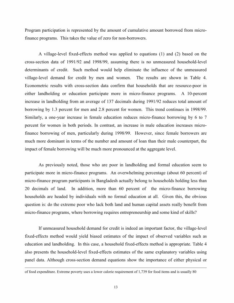
Program participation is represented by the amount of cumulative amount borrowed from micro-

finance programs. This takes the value of zero for non-borrowers.

A village-level fixed-effects method was applied to equations (1) and (2) based on the

cross-section data of 1991/92 and 1998/99, assuming there is no unmeasured household-level

determinants of credit. Such method would help eliminate the influence of the unmeasured

village-level demand for credit by men and women. The results are shown in Table 4.

Econometric results with cross-section data confirm that households that are resource-poor in

either landholding or education participate more in micro-finance programs. A 10-percent

increase in landholding from an average of 137 decimals during 1991/92 reduces total amount of

borrowing by 1.3 percent for men and 2.8 percent for women. This trend continues in 1998/99.

Similarly, a one-year increase in female education reduces micro-finance borrowing by 6 to 7

percent for women in both periods. In contrast, an increase in male education increases micro-

finance borrowing of men, particularly during 1998/99. However, since female borrowers are

much more dominant in terms of the number and amount of loan than their male counterpart, the

impact of female borrowing will be much more pronounced at the aggregate level.

As previously noted, those who are poor in landholding and formal education seem to

participate more in micro-finance programs. An overwhelming percentage (about 60 percent) of

micro-finance program participants in Bangladesh actually belong to households holding less than

20 decimals of land. In addition, more than 60 percent of the micro-finance borrowing

households are headed by individuals with no formal education at all. Given this, the obvious

question is: do the extreme poor who lack both land and human capital assets really benefit from

micro-finance programs, where borrowing requires entrepreneurship and some kind of skills?

If unmeasured household demand for credit is indeed an important factor, the village-level

fixed-effects method would yield biased estimates of the impact of observed variables such as

education and landholding. In this case, a household fixed-effects method is appropriate. Table 4

also presents the household-level fixed-effects estimates of the same explanatory variables using

panel data. Although cross-section demand equations show the importance of either physical or of food expenditure. Extreme poverty uses a lower calorie requirement of 1,739 for food items and is usually 80

14

human resources, this is not the case with the household-level fixed effects method. This means

that unobserved ability, such as the entrepreneurship of a household, matters most in influencing

the demand for micro-credit over time, although landholding and education, perhaps proxy for

such unobserved household attributes, may indicate the participation in a program. In other

words, landholding and education are poor indicators of who participate and how much they

borrow from a micro-finance program among males and females from eligible households. Yet in

other words, even if micro-finance programs have been able to draw participants from the poor

with lower landholding and education, these factors do not matter over time when unobserved

ability such as entrepreneurial ability or other household attributes perhaps matter most in program

participation.

VI. Estimates of poverty impacts on participants

Poverty reduction is an overarching objective of a targeted program such as targeted micro-finance

programs. As the poor with unobserved skills or attributes are likely to participate more in micro-

finance programs, the impact assessments of micro-finance on poverty reduction must take care of

these unobserved factors associated with participation.

The household fixed-effects method, which controls for fixed unobserved attributes of

households participating in such programs, may not yet yield consistent estimates of credit

impacts with panel data when unmeasured determinants (at both household and village level) of

credit vary over time. Also there is another problem to worry about: If credit is measured with

errors (which is likely), this error gets amplified when differencing over time, especially with only

two time periods. This measurement error will impart “attenuation bias” on the credit impact

coefficients, meaning that the impact estimates are biased toward zero. A standard correction for

such bias is the use of instrumental variable (IV) estimation. The IV method is also relevant to

taking care of the problem that arises when the unobserved characteristics are not fixed but time-

varying.

Since it is the accumulated credit or stock of credit that influences consumption, we can

rewrite the outcome equation (suppressing subscripts for male and female) as,

percent below the moderate poverty line.

15

Cijt = Xijtβc + Sijtδb + ηcijt + εc

ijt (5)

where we replaced the credit variable B with stock of credit S. Now for two periods we write the

above consumption equation as,

Cij1 = Xij1βc + Sij1δb + ηcij1 + εc

ij1

Cij2 = Xij2βc + Sij2δb + ηcij2 + εc

ij2

Taking the difference we obtain,

∆Cij = ∆Xijβc + ∆Sijδb + ∆ηcij + ∆εc

ij

Since the difference between the stocks of credit in two periods is in fact the credit reported during

second period, that is B2, we can write the above equation as,

∆Cij = ∆Xijβc + Bij2δb + ∆ηcij + ∆εc

ij (6)

Now for the implementation of IV method, let us write the first-stage equation for the

stock of credit (suppressing subscripts for male, female, household and village) as,

St = Xtβb + Ztγt + εbt

where Z is a set of household and village characteristics distinct from X’s so that they affect S but

not other household outcomes dependent on S. The impact of Z variables on S is allowed to vary

with time because of the possibility of differential effects of instruments over time on credit

demand. For two periods we can write the above equation as,

S1 = X1βb + Z1γ1 + εb1

S2 = X2βb + Z2γ2 + εb2

Taking the difference we obtain,

16

∆S2 = ∆Xβb + Z2γ2 – Z1γ1 + ∆εb

which becomes,

B2 = ∆Xβb + Z2γ2 – Z1γ1 + ∆εb (7)

Selecting appropriate Z variables is a crucial part of this exercise. In order to do that we define a

household-level choice variable which determines whether or not a household has a choice to

participate in a program. A household’s choice in program participation depends on two factors:

whether a credit program operates in the village where the household lives in and whether the

household itself qualifies to participate in the program, based on the landholding criteria (that is if

the household’s landholding is 0.5 acre or less). A male’s or female’s choice to participate in a

program depends not only on whether the village has a program and whether the household

satisfies the land eligibility condition but also whether the village has a male or female group, as

participation is gender-based. The choice variable so defined is considered for both 1991/92 and

1998/99 to take care of the differential impacts of two periods and is then interacted with

household-level exogenous variables and village fixed-effects to get the instruments.

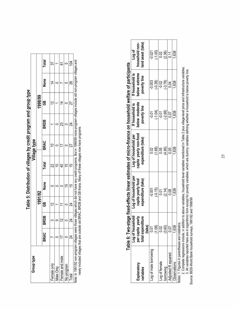
Table 5 shows a distribution of survey villages by male and female choice group. A

common trend is obvious from this table that groups with both males and females have increased

in the program areas over the years. Another interesting phenomenon is expansion of program

outreach in areas that were previously non-program. Although number of villages have increased

from 1991/92 to 1998/99, number of non-program villages with no program has decreased from

15 to 5.

Table 6 presents household fixed-effects IV estimates of program impacts on six

outcomes: per capita total expenditure, per capita food expenditure, per capita non-food

expenditure, the incidence of moderate and extreme poverty, and household non-land asset. The

results are quite interesting. Male borrowing has no impact on household per capita total

expenditure and moderate poverty, but some impact on per capita non-food expenditure. For the

expenditure and non-land asset equations, we used logarithmic equation, in which case the

coefficients of credit measure the response elasticity. In contrast, the poverty incidence equations

17

are log-linear equation, in which case the coefficient on credit measures the probabilistic change in

outcomes with respect to percentage changes in borrowing. Thus, a 10-percent increase in male

borrowing increases household non-food expenditure by 0.2 percent.

In contrast, a 10-percent increase in female borrowing increases household per capita total

expenditure by 0.2 percent, food expenditure by 0.1 percent, non-food expenditure by 0.5 percent

and household non-land asset by 0.2 percent.

Unlike consumption and asset variables which are continuous, the poverty incidence

variables are binomial (meaning 1 if the household is moderately or extremely poor and zero

otherwise). Household fixed-effects method is non-applicable with such discontinuous variables.

Two-stage method is even harder. Thus, we used linear probability functional form to estimate the

impact of borrowing in a two-stage fashion just to indicate the direction of change in these

outcomes due to borrowing. The results support the view that micro-finance borrowing reduces

poverty, especially extreme poverty.

In order to quantify the contribution of micro-finance to poverty reduction, we can

alternatively use the consumption estimates.9 The results of this exercise are shown in the first

two columns of Table 9. The findings indicate that participants’ moderate poverty dropped 8.5

percentage points over the period of seven years, while extreme poverty dropped about 18.2 points

over the same period. Interestingly enough, the returns to borrowing have declined over time.

Based on the panel data estimates, the returns to female borrowing are 10.5 percent, which was 18

percent according to cross-sectional estimates of 1991/92 data. Overall, the results suggest the

following: (1) micro-finance impacts are much stronger for female borrowers than for male

borrowers and that returns to borrowing have declined over time; (2) the impacts on expenditure

are more pronounced for non-food expenditure than for food expenditure; and (3) the poverty

9Since a household’s per capita consumption is directly linked with its poverty status, the impact of micro-credit borrowing on per capita consumption can also be used to determine the total change in household’s poverty status due to micro-credit borrowing. A simulation exercise is done where marginal impact of micro-credit borrowing (in this case only female borrowing as male borrowing has no significant impact) on household per capita expenditure is calculated from the regression output shown in table 6. That marginal impact is used to calculate the increase in participant household’s total consumption due to micro-credit borrowing. This amount when subtracted from the current consumption of participants, gives a pre-borrowing level of consumption and this consumption can be compared with the poverty line to get a pre-borrowing poverty status of the participants.

18

impacts of female borrowing are much stronger in reducing extreme poverty than it is in reducing

moderate poverty at the participant level.

VII. Estimates of spillover and aggregate impacts

The total loan outstanding of micro-finance organizations in Bangladesh was about US$600

million in 1998/99. This indicates a large inflow of micro-funds in the rural areas, which is

expected to make an aggregate impact on the local economy. We have just seen that micro-

finance has sizeable effects on the welfare of borrowing households in terms of raising

consumption and non-land asset as well as in reducing moderate and extreme poverty. But are

these effects felt beyond the program participants? How do we account for estimating micro-

finance effects on non-participants?

The cross-section data estimates of Pitt and Khandker (1998) show the effects of

participation above and beyond the non-participation in a program. A program may affect the non-

participants and, thus spillover effects are non-zero. Only longitudinal data allow us to estimate

the spillover effects. We therefore need panel data to do so. When there are spillover effects,

unobserved village heterogeneity would be correlated with program placement, but the causation

would go from program placement to village unobserved effects, not from village effects to

program placement. This measurement problem implies that the placement of a credit program

may cause a village effect in addition to a pre-existing (time-invariant) village effect.

Cij =β Xij +δ Sij + ηij +µj + Ωj + εij (8)

where Ωj represents the external effects of a program in a village and has the value of zero if no

program is located in the village, µj is unobserved village-level fixed-effect, and ηij is unobserved

household-level fixed-effect. The program effect parameter, δ, estimated with cross-section data

captures all program effects only if Ωj = 0. (None of the village-specific heterogeneity is caused

by programs). If village externalities exist (Ωj ≠ 0), then the spillover effect is not separately

identified from the time-invariant village effect (µj). With panel data, it is possible to estimate the

spillover effect with the following equation:

19

Cijt =β Xijt++δ Sij+ ηij + Ωjt + εijt (9)

We excluded the µ-term, since with panel data, household fixed-effects sweep away the village

effects and make it possible to estimate the impact of Ωjt. Suppose Ωjt is measured by the

aggregate credit obtained in a village, then the spillover effect is measured by the change in

behavior of non-participants due to change in aggregate micro-credit obtained in the village. That

is, for non-participants,

)10(0&,2,1,)(

1

==+++= ∑=

ijtkjtkj

jn

iijtkjtkjt StSXC εηδβ

where k refers to the non-participants of micro-finance programs living in j-th village.

Since measurement errors are diminished with aggregation, there is no need to use a two-

stage method for taking care of attenuation bias with credit variables. The above equation is

estimated by the household fixed-effects method that eliminates also program placement bias. The

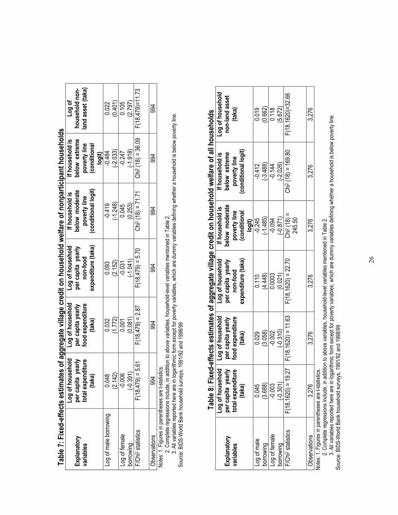
estimated effects of credit on non-participants are presented in Table 7.

The benefits of non-participants depend on the amount of credit obtained by all program

borrowers living in a village. We find an evidence of externality of micro-credit programs. Male

borrowing from micro-finance programs affects the food, non-food, and total per capita

expenditure of non-participants but has no effect on the non-land asset. In contrast, although

female borrowing has no significant effect on consumption of non-participants, it has a substantial

effect on their non-land asset. For instance, a 10-percent increase in aggregate village micro-credit

borrowing by female members increases household non-land asset of non-participants by as much

as 1.1 percent. Micro-finance also affects the poverty incidence among non-participants. The

negative spillover effect on poverty is, however, more pronounced for extreme poverty than for

moderate poverty. The two-stage logit estimates indicate that the probability of reducing extreme

poverty can be as much as 0.09 percentage points. Based on alternative consumption estimates, the

net contribution of female borrowing on poverty is calculated and presented in table 9.

Accordingly, moderate poverty for non-participants declined by 1.1 percentage points and extreme

20

poverty by 4.8 points over the study period because of female borrowing in the village from

micro-finance programs.

We may also assess the aggregate effect of micro-finance by examining the program

effects for an average household by estimating similar equation. For all households we can write:

)11(0&,2,1,)(

1

==+++= ∑=

ijtljtlj

jn

iijtljtljt StSXC εηδβ

where l = i+k. Unlike the earlier equation, every household in the village in this equation is

affected by the same male and female credit irrespective of participation status in a micro-finance

program. A simple household-level fixed-effects method is used to estimate the micro-finance

aggregate effects on welfare of all households living in a village.

Table 8 presents the aggregate micro-finance impact for male and female borrowings. The

results strongly support the view that micro-credit not only affects the welfare of participants and

non-participants but also the aggregate welfare at village level. Male borrowing increases average

household welfare by increasing household total consumption, as well as food and nonfood

consumption, and by reducing extreme poverty, with only a minimal effect on moderate poverty.

Female credit, on the other hand, reduces extreme poverty and increases household non-land asset

for an average household in a village.

Micro-finance operation in a village, therefore, reduces the incidence of extreme poverty

for an average household living in a village but it does not affect the incidence of moderate

poverty. The probability of reducing aggregate extreme poverty is approximately .03 percentage

points for female borrowing and .08 percentage points for male borrowing. However, the net

contribution of female borrowing over the study period (based on alternative consumption

estimates and presented in table 9) is 1.7 percentage points for moderate poverty and 5.5

percentage points. Non-borrowers seem to benefit from micro-finance partly due to the externality

of borrowing by program participants and partly because of externality due to program placement.

Therefore, micro-finance contributes to the overall welfare of the society.

21

VIII. Summary and conclusions

Program evaluation compares outcomes of treatment groups with those of control groups. Finding

control group in a non-experimental setting is very difficult. Traditionally, resorting to instruments

for identifying program effects is done with cross-section data. However, finding good

instruments is equally difficult. Pitt and Khandker (1998) used quasi-experimental method relying

on exogenous eligibility conditions as a way of identifying program effects. Some of the

conditions are restrictive and might not be reliable, for example, the non-enforceability of

landholding criterion for program participation. Results may be sensitive to methods used in

impact assessment. An impact assessment was carried out using a follow-up survey to see the

sensitivity of the findings (see Khandker and Pitt (2002) for details).

This paper carried out a similar exercise by estimating the effects of micro-finance on

consumption, poverty and non-land assets for participants, non-participants, and an average

villager, assuming that micro-finance programs have spillover (externality) effects. The results are

resounding: micro-finance matters a lot for the very poor borrowers and also for the local

economy. In particular, micro-finance programs matter a lot to the poor in raising per capita

consumption, mainly on non-food, as well as household non-land asset. This increases the

probability that the program participants may be able to lift themselves out of poverty. The

welfare impact of micro-finance is also positive for all households, including non-participants,

indicating that micro-finance programs are helping the poor beyond income redistribution with

contribution to local income growth. Programs have spillover effects in local economies, thereby

increasing local village welfare. In particular, we find that micro-finance helps reduce extreme

poverty more than moderate poverty at the village level. Yet the aggregate poverty reduction

effects are not quite substantial to have a large dent on national level aggregate poverty. This

concern brings to the fore the effectiveness of micro-finance as an instrument to solve the problem

of poverty in Bangladesh.

To exhibit a stronger impact on poverty reduction, micro-finance should perhaps go

beyond the provision of financial services. It should find ways to improve the skills of its poor

borrowers to improve their productivity and income. It should also assist its borrowers in

22

marketing and improving the quality of their products. Micro-finance is, however, only one of the

many instruments of poverty reduction. Growth matters too—even more significantly than other

instruments. Investment in human capital and other means to empower the poor also matter. To

achieve substantial poverty reduction, the other avenues must be explored as well.

23

Tabl

e 1: D

istrib

utio

n of

hou

seho

lds b

y pro

gram

par

ticip

atio

n Pr

ogra

m p

artic

ipat

ion

stat

us

1991

/92 su

rvey

19

98/99

surv

ey

Gram

een B

ank m

embe

rs 8.5

14

.3 BR

AC m

embe

rs 11

.6 9.3

BR

DB R

D-12

mem

bers

6.2

3.6

Othe

r NGO

mem

bers

0 11

.1 Mu

ltiple

prog

ram

memb

ers

0 7.4

Ta

rget

non-

partic

ipants

40

.3 25

.6 No

n-tar

get h

ouse

holds

33

.4 28

.8 No

. of o

bser

vatio

ns

1,769

2,5

99

N

ote: O

ther N

GO ho

useh

olds i

nclud

e mem

bers

of AS

A, P

ROSH

IKA,

GSS

, You

th De

velop

ment

and o

ther s

mall N

GOs.

Ta

ble 2

: Hou

seho

ld p

artic

ipat

ion

in m

icro-

cred

it pr

ogra

ms

1991

/92 su

rvey

19

98/99

surv

ey

Land

hold

ing

(dec

imal)

Pa

rticip

atio

n ra

te

in ea

ch

landh

oldi

ng g

roup

Dist

ribut

ion

of

parti

cipan

ts b

y

landh

oldi

ng g

roup

Parti

cipat

ion

rate

in

each

land

hold

ing

grou

p

Dist

ribut

ion

of

parti

cipan

ts b

y

landh

oldi

ng g

roup

Parti

cipat

ion

rate

in m

ultip

le pr

ogra

ms i

n ea

ch

landh

oldi

ng g

roup

0

56.4

8.3

58.8

10.9

12.5

1-20

33

.1 53

.8 58

.0 49

.8 15

.8

21-5

0 29

.5 15

.3 48

.3 14

.5 13

.3

51-1

00

24.3

9.4

43.7

11.3

20.3

101-

250

16.0

10.3

35.0

10.6

18.1

251+

7.1

2.9

12

.0 2.9

21

.8

All h

ouse

holds

26

.0 10

0.0

45.6

100.0

16

.1

Obse

rvatio

ns

1,769

89

4 2,5

99

1,630

1,6

30

24

Tabl

e 3: S

umm

ary s

tatis

tics o

f out

com

e and

cred

it va

riabl

es

1991

/92

1998

/99

Varia

bles

Pr

ogra

m

parti

cipan

ts

Targ

et n

on-

parti

cipan

ts

Non-

targ

et

grou

p Al

l ho

useh

olds

Pr

ogra

m

parti

cipan

ts

Targ

et n

on-

parti

cipan

ts

Non-

targ

et

grou

p Al

l ho

useh

olds

Ma

le bo

rrowi

ng (t

aka)

2,7

30.0

(6,34

1.1)

0 0

705.7

(3

,437.5

) 2,1

98.3

(8,11

2.7)

0 0

1,173

.3 (6

,007.9

) Fe

male

borro

wing

(tak

a)

5,311

.6 (7

,573.4

) 0

0 1,3

73.0

(4,49

7.5)

12,00

8.7

(18,3

71.9)

0

0 6,3

67.4

(14,6

58.1)

Ho

useh

old pe

r cap

ita ye

arly

total

e

xpen

ditur

e (tak

a)

3,923

.4 (1

,566.6

) 3,8

38.0

(1,79

5.5)

5,586

.0 (3

,442.8

) 4,4

62.7

(2,57

8.7)

5,276

.9 (3

,490.4

) 4,7

82.0

(2,97

7.9)

7,587

.6 (6

,317.4

) 5,8

10.1

(4,50

2.5)

Hous

ehold

per c

apita

year

ly fo

od (t

aka)

3,0

57.4

(786

.3)

3,018

.7 (9

48.7)

3,6

29.2

(1,05

0.6)

3,239

.2 (9

87.9)

3,5

26.9

(1,30

4.2)

3,466

.0 (1

,634.9

) 4,4

00.8

(2,15

6.3)

3,753

.4 (1

,687.8

) Ho

useh

old pe

r cap

ita ye

arly

nonf

ood

(taka

) 86

6.0

(1,09

8.8)

819.3

(1

,118.6

) 1,9

56.8

(2,87

5.2)

1,223

.5 (1

,982.8

) 1,7

50.0

(2,77

0.7)

1,316

.0 (1

,753.9

) 3,1

86.8

(5,28

7.0)

2,056

.7 (3

,575.1

) He

ad co

unt r

atio f

or m

oder

ate po

verty

0.9

03

(0.29

6)

0.896

(0

.306)

0.7

02

(0.45

8)

0.831

(0

.375)

0.7

05

(0.45

6)

0.747

(0

.435)

0.5

03

(0.50

1)

0.658

(0

.474)

He

ad co

unt r

atio f

or ex

treme

pov

erty

0.526

(0

.500)

0.5

81

(0.49

4)

0.245

(0

.431)

0.4

51

(0.49

8)

0.343

(0

.475)

0.4

54

(0.49

9)

0.200

(0

.401)

0.3

26

(0.46

9)

Hous

ehold

non-

land a

sset

(taka

)

17,89

1.9

(25,6

06.1)

14

,251.3

(2

7,122

.4)

53,91

4.7

(85,1

90.3)

28

,867.4

(5

7,331

.1)

31,94

1.4

(100

,778.0

) 29

,044.5

(6

9,022

.2)

72,19

9.2

(109

,925.1

) 42

,358.1

(9

9,700

.5)

Obse

rvatio

ns

824

567

247

1,638

1,1

22

279

237

1,638

N

ote: F

igure

s in p

aren

these

s are

stan

dard

devia

tions

.

Tabl

e 4: F

ixed-

effe

cts T

obit

estim

ates

of m

icro-

cred

it bo

rrowi

ng

Villa

ge-le

vel f

ixed

effe

cts

1991

/92 d

ata

1998

/99 d

ata

Hous

ehol

d-lev

el fix

ed ef

fect

s Pa

nel d

ata

Expl

anat

ory v

ariab

les

Log

of m

ale

borro

wing

Lo

g of

fem

ale

borro

wing

Lo

g of

male

bo

rrowi

ng

Log

of fe

male

bo

rrowi

ng

Log

of m

ale

borro

wing

Lo

g of

fem

ale

borro

wing

Ma

ximum

educ

ation

of

hous

ehold

male

(yea

rs)

0.03

(0.70

) -0

.003

(-0.05

) 0.0

3 (1

.72)

0.003

(0

.08)

0.05

(1

.51)

-0

.04

(-1.

01)

Maxim

um ed

ucati

on of

ho

useh

old fe

male

(year

s) -0

.04

(-1.10

) -0

.07

(-1.63

) -0

.02

(-0.43

) -0

.06

(-1.74

) -0

.01

(-0.

43)

0.01

(0

.36)

Lo

g of h

ouse

hold

land a

ssets

(d

ecim

al)

-0.13

(-2

.55)

-0.28

(-4

.56)

-0.09

(-2

.21)

-0.55

(-8

.38)

-0.0

1 (-

0.13

) -0

.15

(-1.

22)

F-sta

tistic

s 3.1

4 7.0

5 3.4

2 13

.40

5.51

11.98

Nu

mber

of ob

serva

tions

1,7

69

1,769

2,2

90

2,290

3,2

76

3,276

N

otes:

1. Fig

ures

in pa

renth

eses

are t

-stati

stics

.

2. C

omple

te re

gres

sions

inclu

de, in

addit

ion to

varia

bles g

iven,

sex a

nd ag

e of h

ouse

hold

head

, if pa

rents

; bro

thers

and s

ister

s of h

ouse

hold

head

;

ho

useh

old he

ad’s

spou

se ow

n lan

d.

25

Tabl

e 5: D

istrib

utio

n of

villa

ges b

y cre

dit p

rogr

am an

d gr

oup

type

Vi

llage

type

19

91/92

19

98/99

Gr

oup

type

BRAC

BR

DB

GB

None

To

tal

BRAC

BR

DB

GB

None

To

tal

Fema

le on

ly 7

3 12

0

22

10

1 12

14

37

Ma

le On

ly 0

9 1

0 10

0

0 1

0 1

Fema

le an

d male

17

12

11

0

40

17

23

14

7 61

No

prog

ram

0 0

0 15

15

0

0 0

5 5

Total

24

24

24

15

15

27

24

27

26

10

4 N

ote: In

1991

/92 no

n-pr

ogra

m vil

lages

wer

e tho

se vi

llage

s whic

h did

not h

ave a

ny cr

edit p

rogr

ams.

But in

1998

/99 no

ne-p

rogr

am vi

llage

s inc

lude o

ld no

n-pr

ogra

m vil

lages

and

ne

wly i

nclud

ed vi

llage

s tha

t are

outsi

de ol

d BRA

C, B

RDB

and G

B tha

na. M

any o

f thes

e villa

ges n

ow ha

ve pr

ogra

ms

Tabl

e 6: T

wo-s

tage

fixe

d-ef

fect

s lin

ear e

stim

ates

of m

icro-

finan

ce o

n ho

useh

old

welfa

re o

f par

ticip

ants

Expl

anat

ory

varia

bles

Log

of h

ouse

hold

pe

r cap

ita y

early

to

tal e

xpen

ditu

re

(taka

)

Log

of h

ouse

hold

per

ca

pita

year

ly fo

od

expe

nditu

re (t

aka)

Log

of h

ouse

hold

per

ca

pita

yea

rly n

on-fo

od

expe

nditu

re (t

aka)

If ho

useh

old

is be

low

mod

erat

e po

verty

line

If ho

useh

old

is be

low

extre

me

pove

rty lin

e

Log

of

hous

ehol

d no

n-lan

d as

set (t

aka)

Log o

f male

borro

wing

0.0

1 (1

.08)

-0.00

1 (-0

.15)

0.02

(1.68

) -0

.01

(-1.04

) -0

.003

(-0.38

) -0

.021

(-1.00

) Lo

g of fe

male

borro

wing

0.0

2 (3

.60)

0.01

(2.14

) 0.0

5 (4

.95)

-0.01

(-2

.68)

-0.02

(-3

.78)

0.02

(2.36

) Ad

justed

R sq

uare

d 0.0

7 0.0

80.0

50.0

70.0

40.1

1Ob

serva

tions

1,6

38

1,638

1,6

38

1,638

1,6

38

1,638

N

otes:

1. Fig

ures

in pa

renth

eses

are t

-stati

stics

.

2. C

omple

te re

gres

sions

inclu

de, in

addit

ion to

abov

e var

iables

, hou

seho

ld lev

el va

riable

s men

tione

d in T

able

2 plus

villa

ge-le

vel p

rice a

nd in

frastr

uctur

e var

iables

.

3. A

ll var

iables

repo

rted h

ere a

re in

loga

rithmi

c for

m ex

cept

for po

verty

varia

bles,

which

are d

ummy

varia

bles d

efinin

g whe

ther a

hous

ehold

is be

low po

verty

line.

So

urce

: BID

S-W

orld

Bank

hous

ehold

surve

ys, 1

991/9

2 and

1998

/99

26

Ta

ble 7

: Fixe

d-ef

fect

s est

imat

es o

f agg

rega

te vi

llage

cred

it on

hou

seho

ld w

elfar

e of n

onpa

rticip

ant h

ouse

hold

s

Expl

anat

ory

varia

bles

Log

of h

ouse

hold

pe

r cap

ita y

early

to

tal e

xpen

ditu

re

(taka

)

Log

of h

ouse

hold

pe

r cap

ita ye

arly

food

expe

nditu

re

(taka

)

Log

of h

ouse

hold

pe

r cap

ita y

early

no

n-fo

od

expe

nditu

re (t

aka)

If ho

useh

old

is be

low

mod

erat

e po

verty

line

(con

ditio

nal lo

git)

If ho

useh

old

is be

low

extre

me

pove

rty lin

e (c

ondi

tiona

l lo

git)

Log

of

hous

ehol

d no

n-lan

d as

set (t

aka)

Log o

f male

borro

wing

0.0

48

(2.14

2)

0.032

(1

.772)

0.0

93

(2.15

2)

-0.41

9 (-1

.248)

-0

.484

(-2.03

3)

0.022

(0

.401)

Lo

g of fe

male

borro

wing

-0

.006

(-0.39

1)

0.001

(0

.081)

-0

.031

(-1.04

1)

0.045

(0

.253)

-0

.247

(-1.91

8)

0.105

(2

.797)

F/

Chi2 s

tatist

ics

F(18

,479)

= 5.

61

F(

18,47

9) =

2.87

F(18

,479)

= 5.

70

Ch

i2 (18

) = 71

.71

Ch

i2 (18

) = 36

.09

F(

18,47

9)=1

1.73

Ob

serva

tions

99

4 99

4 99

4 99

4 99

4 99

4

Notes

: 1. F

igure

s in p

aren

these

s are

t-sta

tistic

s.

2. C

omple

te re

gres

sions

inclu

de, in

addit

ion to

abov

e var

iables

, hou

seho

ld-lev

el va

riable

s men

tione

d in T

able

2.

3

. All v

ariab

les re

porte

d her

e are

in lo

garith

mic f

orm

exce

pt for

pove

rty va

riable

s, wh

ich ar

e dum

my va

riable

s defi

ning w

hethe

r a ho

useh

old is

below

pove

rty lin

e.

S

ource

: BID

S-W

orld

Bank

hous

ehold

surve

ys, 1

991/9

2 and

1998

/99

Tabl

e 8: F

ixed-

effe

cts e

stim

ates

of a

ggre

gate

villa

ge cr

edit

on h

ouse

hold

welf

are o

f all h

ouse

hold

s

Expl

anat

ory

varia

bles

Log

of h

ouse

hold

pe

r cap

ita y

early

to

tal e

xpen

ditu

re

(taka

)

Log

of h

ouse

hold

pe

r cap

ita ye

arly

food

expe

nditu

re

(taka

)

Log

of h

ouse

hold

pe

r cap

ita y

early

no

n-fo

od

expe

nditu

re (t

aka)

If ho

useh

old

is be

low

mod

erat

e po

verty

line

(con

ditio

nal

logi

t)

If ho

useh

old

is be

low

extre

me

pove

rty lin

e (c

ondi

tiona

l logi

t)

Log

of h

ouse

hold

no

n-lan

d as

set

(taka

)

Log o

f male

bo

rrowi

ng

0.045

(3

.688)

0.0

29

(3.05

8)

0.110

(4

.448)

-0

.245

(-1.48

5)

-0.41

2 (-3

.488)

0.0

19

(0.66

2)

Log o

f fema

le bo

rrowi

ng

-0.00

3 (-0

.301)

-0

.002

(-0.31

0)

0.000

3 (0

.021)

-0

.094

(-0.87

1)

-0.14

4 (-2

.026)

0.1

18

(5.67

2)

F/Ch

i2 stat

istics

F(

18,16

20) =

19.27

F(18

,1620

) = 11

.63

F(

18,16

20) =

22.70

Chi2 (

18) =

24

5.50

Chi2 (

18) =

169.8

0

F(18

,1620

)=32

.66

Obse

rvatio

ns

3,276

3,2

76

3,276

3,2

76

3,276

3,2

76

Note

s: 1.

Figur

es in

pare

nthes

es ar

e t-st

atisti

cs.

2.

Com

plete

regr

essio

ns in

clude

, in ad

dition

to ab

ove v

ariab

les, h

ouse

hold-

level

varia

bles m

entio

ned i

n Tab

le 2.

3. A

ll var

iables

repo

rted h

ere a

re in

loga

rithmi

c for

m ex

cept

for po

verty

varia

bles,

which

are d

ummy

varia

bles d

efinin

g whe

ther a

hous

ehold

is be

low po

verty

line.

S

ource

: BID

S-W

orld

Bank

hous

ehold

surve

ys, 1

991/9

2 and

1998

/99

27

Ta

ble 9

: Sim

ulat

ed im

pact

of m

icro-

cred

it bo

rrowi

ng o

n po

verty

Parti

cipan

ts

Non-

parti

cipan

ts

All h

ouse

hold

s Po

verty

indi

cato

rs

Befo

re

borro

wing

Af

ter

borro

wing

Be

fore

vil

lage-

level

aggr

egat

e bo

rrowi

ng

Afte

r vil

lage-

level

aggr

egat

e bo

rrowi

ng

Befo

re

villag

e-lev

el ag

greg

ate

borro

wing

Afte

r vil

lage-

level

aggr

egat

e bo

rrowi

ng

Head

coun

t rati

o for

mod

erate

pove

rty

85.5

77.0

73.9

72.8

76.2

74.5

Head

coun

t rati

o for

extre

me po

verty

58

.5 40

.3 42

.7 37

.9 44

.3 38

..8

Obse

rvatio

ns

1,946

1,3

30

3,276

Sou

rce: B

IDS-

Wor

ld Ba

nk ho

useh

old su

rveys

, 199

1/92 a

nd 19

98/99

28

Bibliography

Adams, D.W., and J.D. Von Pischke. 1992. “Microenterprise Credit Programs: Déjà

vu.” World Development 20 (October):1463-70.

Coleman, B.E. 1999. “The Impact of group lending in Northeast Thailand.” Journal of

Development Economics 60 (October):105-141.

Hashemi, Syed M., Sidney R. Schuler and Ann P. Riley. 1996. “Rural Credit Programs

and Women’s Empowerment in Bangladesh.” World Development 24 (April):635-

53.

Hossain, Mahabub. 1988. “Credit for Alleviation of Rural Poverty: The Grameen Bank

in Bangladesh.” IFPRI Research Report 65. International Food Policy Research

Institute, Washington, D.C.

Jalan, Jyotsna and Martin Ravallion (2002). “Geographic Poverty Traps? A Micro

Model of Consumption Growth in Rural China.” World Bank (mimeo)

Khalily, M. B., M. O. Imam, and S. A. Khan. 2000. "Efficiency and Sustainability of

Formal and Quasi-formal Micro-finance Programs-- An Analysis of Grameen

Bank and ASA." In Rushidan I. Rahman and Shahidur R. Khandker, eds., The

Bangladesh Development Studies, A Special Issue on Microfinance and

Development: Emerging Issues 26(June/September): 103-146.

Khandker, Shahidur R. and Mark M. Pitt. 2002. “The Impact of Group-Based Credit

on Poor Households: An Analysis of Panel Data from Bangladesh.” (mimeo)

Khandker, Shahidur R. 1988. Fighting Poverty with Microcredit: Experience in

Bangladesh. New York, NY: Oxford University Press for the World Ban k.

Lalonde, R. 1986. "Evaluating the Econometric Evaluations of Training Programs with

Experimental Data." American Economic Review 76: 604-620.

Morduch, J. 1998. “Does Microfinance Really Help the Poor? New Evidence from

Flagship Programs in Bangladesh.” (unpublished mimeo).

Morduch, J. 1999. “The Role of Subsidies in Microfinance: Evidence from the Grameen

Bank.” Journal of Development Economics 60 (October): 229-248.

Pitt, Mark M. 1999. "Reply to Jonathan Morduch's 'Does Microfinance Really Help the

29

Poor? New Evidence from Flagship Programs in Bangladesh'." (unpublished

manuscript).

Pitt, Mark M. , and Shahidur. R. Khandker. 1998. “The Impact of Group-Based Credit

Programs on Poor Households in Bangladesh: Does the Gender of Participants

Matter?” Journal of Political Economy 106 (October): 958-96.

Rahman, Rushidan I. 1996. “Impact of Grameen Krishi Foundation on the

Socioeconomic Condition of Rural Households”, BIDS Working paper No. 7,

BIDS, Bangladesh Institute of Development Studies, Dhaka.

Ravallion, Martin, and Binayak Sen. 1995. When Methods Matter: Towards a

Resolution of the Debate about Bangladesh’s Poverty Measures. Policy working

paper 1259, World Bank, Washington, D.C.

Schuler, Sidney R., and Syed M. Hashemi. 1994. “Credit Programs, Women’s

Empowerment, and Contraceptive Use in Rural Bangladesh.” Studies in Family

Planning 25 (March/April):65-76.

Yaron, Jacob. 1994. “What Makes Rural Finance Institutions Successful?” The World

Bank Research Observer 9 (1):49-70.

World Bank 2001. World Development Report, 2000/2001: Attacking Poverty,

Washington, D.C.

30

Appendix Table A: Summary statistics of explanatory variables

Variables 1991/92 1998/99 Whole sample Cumulative male borrowing ( taka) 705.68

(3,437.55) 1,173.27

(6,007.89) 939.48

(4,899.30) Cumulative female borrowing ( taka) 1,372.98

(4,497.54) 6,367.38

(14,658.06) 3,870.18

(11,124.09) Program duration of males (years) 0.39

(1.38) 0.80

(2.51) 0.59

(2.04) Program duration of females (years) 0.67

(1.61) 2.22

(3.51) 1.45

(2.84) Village aggregate male borrowing (taka) 30,678

(48,701) 49,051

(111,060) 39,628

(86,470) Village aggregate female borrowing 47,983

(62,978) 222,971

(316,508) 136,584

(244,141) Highest grade completed by household head (years) 2.77

(3.68) 2.49

(3.64) 2.63

(3.66) Sex of household head (male=1, female=0) 0.95

(0.21) 0.87

(0.34) 0.91

(0.28) Age of household head (years) 41.29

(12.94) 48.50

(13.18) 44.89

(13.55) Maximum education by household male (years) 3.44

(3.93) 4.57

(4.53) 4.00

(4.28) Maximum education by household male (years) 1.79

(3.04) 3.02

(3.83) 2.40

(3.51) No adult male lives in household 0.03

(0.17) 0.03

(0.16) 0.03

(0.17) No adult male lives in household 0.01

(0.11) 0.01

(0.08) 0.01

(0.10) Household land (decimals) 130.03

(316.56) 133.05

(325.85) 131.54

(321.19) No spouse lives in household 0.11

(0.31) 0.17

(0.37) 0.14

(0.34) Parents of household head own land 0.21

(0.41) 0.17

(0.37) 0.19

(0.39) Brothers of household head own land 0.39

(0.49) 0.37

(0.48) 0.38

(0.49) Sisters of household head own land 0.40

(0.49) 0.31

(0.46) 0.35

(0.48) Parents of household head’s spouse own land 0.35

(0.48) 0.32

(0.47) 0.34

(0.47) Brothers of household head’s spouse own land 0.39

(0.49) 0.38

(0.49) 0.39

(0.49) Sisters of household head’s spouse own land 0.40

(0.49) 0.31

(0.46) 0.35

(0.48) If village is accessed by road all year 0.94

(0.23) 0.85

(0.36) 0.90

(0.31) Proportion of village land irrigated 0.44

(0.31) 0.57

(0.32) 0.51

(0.32) If village has electricity 0.50

(0.50) 0.60

(0.49) 0.55

(0.50) Village price of rice 9.71

(0.97) 10.38 (1.68)

10.04 (1.41)

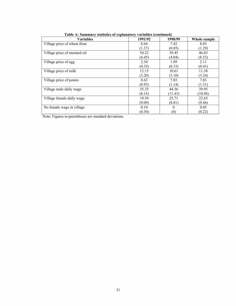
31

Table A: Summary statistics of explanatory variables (continued)

Variables 1991/92 1998/99 Whole sample Village price of wheat flour 8.64

(1.37) 7.42

(0.85) 8.03

(1.29) Village price of mustard oil 54.22

(4.45) 39.45 (4.04)

46.83 (8.52)

Village price of egg 2.34 (0.35)

1.89 (0.33)

2.11 (0.41)

Village price of milk 12.15 (3.20)

10.61 (3.10)

11.38 (3.24)

Village price of potato 8.63 (0.93)

7.03 (1.14)

7.83 (1.31)

Village male daily wage 35.35 (8.15)

44.56 (11.43)

39.95 (10.94)

Village female daily wage 19.59 (9.09)

25.71 (8.81)

22.65 (9.46)

No female wage in village 0.10 (0.30)

0 (0)

0.05 (0.22)

Note: Figures in parentheses are standard deviations.