HAL Id: hal-00587663https://hal.archives-ouvertes.fr/hal-00587663v2

Preprint submitted on 30 Nov 2011

HAL is a multi-disciplinary open accessarchive for the deposit and dissemination of sci-entific research documents, whether they are pub-lished or not. The documents may come fromteaching and research institutions in France orabroad, or from public or private research centers.

L’archive ouverte pluridisciplinaire HAL, estdestinée au dépôt et à la diffusion de documentsscientifiques de niveau recherche, publiés ou non,émanant des établissements d’enseignement et derecherche français ou étrangers, des laboratoirespublics ou privés.

Ecosystem Viable YieldsMichel de Lara, Eladio Ocana Anaya, Ricardo Oliveros–Ramos, Jorge Tam

To cite this version:Michel de Lara, Eladio Ocana Anaya, Ricardo Oliveros–Ramos, Jorge Tam. Ecosystem Viable Yields.2011. �hal-00587663v2�

Ecosystem Viable Yields

Michel De Lara∗ Eladio Ocana † Ricardo Oliveros-Ramos ‡ Jorge Tam ‡

November 30, 2011

Abstract

The World Summit on Sustainable Development (Johannesburg, 2002) encouraged the appli-

cation of the ecosystem approach by 2010. However, at the same Summit, the signatory States

undertook to restore and exploit their stocks at maximum sustainable yield (MSY), a concept

and practice without ecosystemic dimension, since MSY is computed species by species, on the

basis of a monospecific model. Acknowledging this gap, we propose a definition of “ecosystem

viable yields” (EVY) as yields compatible i) with guaranteed biological safety levels for all time

and ii) with an ecosystem dynamics. To the difference of MSY, this notion is not based on

equilibrium, but on viability theory, which offers advantages for robustness. For a generic class

of multispecies models with harvesting, we provide explicit expressions for the EVY. We apply

our approach to the anchovy–hake couple in the Peruvian upwelling ecosystem.

Key words: control theory; state constraints; viability; yields; ecosystem management; Peru-

vian upwelling ecosystem.

1 Introduction

Following the World Summit on Sustainable Development (Johannesburg, 2002), the signatory

States undertook to restore and exploit their stocks at maximum sustainable yield (MSY, see

∗Universite Paris–Est, CERMICS, 6–8 avenue Blaise Pascal, 77455 Marne la Vallee Cedex 2, France. Correspond-

ing author: delara@cermics.enpc.fr, fax +33164153586†IMCA-FC, Universidad Nacional de Ingenierıa, Calle los Biologos 245, Lima 12-Peru. eocana@imca.edu.pe, fax

+511349-9838‡IMARPE, Instituto del Mar del Peru, Centro de Investigaciones en Modelado Oceanografico y Biologico Pesquero

(CIMOBP), Apartado 22, Callao–Peru. jtam@imarpe.gob.pe, roliveros@imarpe.gob.pe, fax +5114535053

1

(Clark, 1990)). Though being criticized for decades, MSY remains a reference. Criticisms of MSY,

like (Larkin, 1977), point out that MSY relies upon a single variable stock description (the species

biomass), without age structure nor interactions with other species; what is more, computations

are made at equilibrium. In fisheries, one of the more elaborate method of fixing quotas, the ICES

(International Council for the Exploration of the Sea) precautionary approach (ICES, 2004), does

not assume equilibrium (it projects abundances one year ahead) and assumes age structure; it

remains however based on a monospecific dynamical model. Thus, in fisheries, yields are usually

defined species by species.

On the other hand, more and more emphasis is put on multispecies models (Hollowed, Bax,

Beamish, Collie, Fogarty, Livingston, Pope, and Rice, 2000) and on ecosystem management. For in-

stance, the World Summit on Sustainable Development encouraged the application of the ecosystem

approach by 2010. Also, sustainability is a major goal of international agreements and guidelines

to fisheries management (FAO, 1999; ICES, 2004).

Our interest is in providing conceptual insight as what could be sustainable yields for ecosystems.

In this, we follow the vein of (Katz, Zabel, Harvey, Good, and Levin, 2003) which introduces the

concept of Ecologically Sustainable Yield (ESY), or of (Chapel, Deffuant, Martin, and Mullon,

2008) which defines yield policies in a viability approach. A general discussion on the ecosystem

approach to fisheries may be found in (Garcia, Zerbi, Aliaume, Chi, and Lasserre, 2003).

Our emphasis is on providing formal definition and practical methods to design and compute

such yields. For this purpose, our approach is not based on equilibrium calculus, nor on intertem-

poral discounted utility maximization but on the so-called viability theory, as follows.

On the one hand, the ecosystem is described by a dynamical model controlled by harvesting.

On the other hand, building upon (Bene, Doyen, and Gabay, 2001), constraints are imposed:

catches are expected to be above given production minimal levels, and biomasses above safety

biological minimal levels. Sustainability is here defined as the property that such constraints can

be maintained for all time by appropriate harvesting strategies.

Such problems of dynamic control under constraints refer to viability (Aubin, 1991) or invariance

(Clarke, Ledayev, Stern, and Wolenski, 1995) frameworks, as well as to reachability of target sets

or tubes for nonlinear discrete time dynamics in (Bertsekas and Rhodes, 1971).

We consider sustainable management issues formulated within such framework as in (Bene,

2

Doyen, and Gabay, 2001; Bene and Doyen, 2003; Eisenack, Sheffran, and Kropp, 2006; Mullon,

Cury, and Shannon, 2004; Rapaport, Terreaux, and Doyen, 2006; De Lara, Doyen, Guilbaud, and

Rochet, 2007; De Lara and Doyen, 2008; Chapel, Deffuant, Martin, and Mullon, 2008).

A viable state is an initial condition for the ecosystem dynamical system such that appropriate

harvesting rules may drive the system on a sustainable path by maintaining catches and biomasses

above their respective production and biological minimal levels. We provide a way to characterize

production minimal levels (yields) such that the present initial conditions are a viable state. These

yields are sustainable in the sense that they can be indefinitely guaranteed, while making possible

that the ecosystem remains in an ecologically viable zone; we coin them ecosystem viable yields

(EVY).

Thus, the EVY can be seen as an extension of the MSY concept in two directions: 1) from

equilibrium to viability (more robust); 2) from monospecies to multispecies models. The second

claim is obvious because, as we have recalled at the beginning, the MSY relies upon a single variable

stock description (the species biomass), without interactions with other species. As for the first,

recall that the MSY is the largest constant yield that can be taken from a single species stock over

an indefinite period. By contrast, EVY are guaranteed yields, but they are not necessarily the

annual catches. Indeed, it is by an adaptive catch policy (depending on the states of the stocks)

that we shall be able to display yields indefinitely above the EVY. This is why we say that EVY

are guaranteed yields, in the sense that catches cannot fall below the EVY. Viability can be seen

as a robust extension of equilibrium: yields are not supposed to be sustained by applying fixed

stationary catches, but are minimal levels which can be guaranteed by means of adaptive catch

policies.

The paper is organized as follows. In Section 2, we introduce generic harvested nonlinear ecosys-

tem models, and we present how preservation and production constraints are modelled. Thanks

to an explicit description of viable states, we are able to characterize sustainable yields. These

latter are not defined species by species, but depend on the whole ecosystem dynamics and on all

biological minimal levels. In Section 3, an illustration in ecosystem management and numerical

applications are given for the hake–anchovy couple in the Peruvian upwelling ecosystem between

the years 1971 and 1981. We conclude in Section 4 with possible extensions of the notion of ecosys-

tem viable yields, on the one hand, to more general ecosystem models and, on the other hand, to

3

bio-economic models so as to incorporate some economic considerations. We also discuss the limits

of the EVY concept. In the appendix, Section A is devoted to recalls on discrete–time viability and

its possible use for sustainable management, while Section B contains the mathematical proofs.

2 Ecosystem viable yields

After a brief recall on the notion of maximum sustainable yield (for monospecific models), we

introduce a class of generic harvested nonlinear ecosystem models, then present how to define

maximum sustainable yields for this class. Next, we provide an explicit description of viable states,

for which production and biological constraints can be guaranteed for all times under appropriate

management. This makes possible to define ecosystem viable yields, compatible with biological

and conservation constraints. We end up discussing relations between ecosystem viable yields and

maximum sustainable yields.

2.1 A brief recall on maximum sustainable yield

We briefly sketch the principles leading to the notion of maximum sustainable yield (MSY) (see

(Clark, 1990) in continuous time and (De Lara and Doyen, 2008) in discrete time).

Consider a single population described by its total biomass B(t) at time t. Suppose that the

time evolution of the biomass is given by a dynamical equation, a differential equation B(t) =

Biolc

(

B(t))

in continuous time or a difference equation B(t+ 1) = Biold

(

B(t))

in discrete time.

From this, build a Schaefer model (Schaefer, 1954) by substracting a catch term h(t), giving B(t) =

Biolc

(

B(t))

− h(t) or B(t+ 1) = Biold

(

B(t)− h(t))

. In general, to each biomass level Be (below

the carrying capacity) corresponds a catch level he = Sust(Be) for which the biomass Be is at

equilibrium, solution of Biolc(

Be

)

− he = 0 or Biold(

Be − he)

= Be. The maximum sustainable

yield is the largest of such equilibrium catches: msy = maxBeSust(Be).

2.2 Ecosystem biomass dynamical model

For simplicity, we consider a model with two species, but it can be easiliy extended to N species in

interaction. Each species is described by its biomass: the two–dimensional state vector (y, z) repre-

sents the biomasses of both species. The two–dimensional control (v,w) comprises the harvesting

4

effort for each species, respectively. The catches are thus vy and wz (measured in biomass).1 The

discrete–time control system we consider is

y(t+ 1) = y(t)Ry

(

y(t), z(t), v(t))

,

z(t+ 1) = z(t)Rz

(

y(t), z(t), w(t))

,(1)

where t stand for time (typically, periods are years), and where Ry : R3 → R and Rz : R3 → R are

two functions representing growth factors (the growth rates being Ry − 1 and Rz − 1). This model

is generic in that no explicit or analytic assumptions are made on how the growth factors Ry and

Rz indeed depend upon both biomasses (y, z).

In the above model, each species is harvested by a specific device: one species, one harvesting

effort. This covers the multioutput settings case (e.g. several species in trophic interactions and

targeted by the same fishing gear). Indeed, for this it suffices to state that both efforts are identical:

v(t) = w(t) for all t = t0, t0 + 1, . . ..

2.3 Preservation and production sustainability

We now propose to define sustainability as the ability to respect preservation and production

minimal levels for all times, building upon the original approach of (Bene, Doyen, and Gabay,

2001). Let us be given

• on the one hand, minimal biomass levels B♭y ≥ 0, B♭

z ≥ 0, one for each species,

• on the other hand, minimal catch levels C♭y ≥ 0, C♭

z ≥ 0, one for each species.

A couple (y0, z0) of initial biomasses is said to be a viable state if there exist appropriate

harvesting efforts (controls)(

v(t), w(t))

, t = t0, t0 +1, . . . such that the state path(

y(t), z(t))

, t =

t0, t0 + 1, . . . starting from(

y(t0), z(t0))

= (y0, z0) satisfies the following goals:

• preservation (minimal biomass levels)

biomasses: y(t) ≥ B♭y , z(t) ≥ B♭

z , ∀t = t0, t0 + 1, . . . (2)

1In fact, any expression of the form c(y, v), instead of vy, would fit for the catches in the following Proposition 2

as soon as v 7→ c(y, v) is strictly increasing and goes from 0 to +∞ when v goes from 0 to +∞. The same holds for

d(z, w) instead of wz.

5

• and production requirements (minimal catch levels)

catches: v(t)y(t) ≥ C♭y , w(t)z(t) ≥ C♭

z , ∀t = t0, t0 + 1, . . . (3)

The set of all viable states is called the viability kernel (Aubin, 1991). Characterizing viable states

makes it possible to test whether or not minimal biomasses and catches can be guaranteed for all

time.

Here, by guaranteed, we mean that the yields have to indefinitely above the EVY, as reflected in

the inequalities (2) and (3). We insist on the fact that, in the above definition of viable states, we

say “there exist appropriate harvesting efforts (controls)”: that is, to guarantee the EVY, we need

to resort to adaptive catch policies (depending on the states of the stocks as in Corollary 6 in the

Appendix). Viability can be seen as a robust extension of equilibrium: yields are not supposed to

be sustained by applying fixed stationary catches, but are minimal levels which can be guaranteed

by means of adaptive catch policies.

Notice that, in the multioutput settings case, we need to add the constraint v(t) = w(t) for all

t = t0, t0+1, . . .. Therefore, with an additional constraint, the set of viable states in the multioutput

settings case will be smaller than the one considered above.

The following definition summarizes useful and natural properties required for the growth factors

in the ecosystem model.

Definition 1 We say that growth factors Ry and Rz in the ecosystem model (1) are nice if

the function Ry : R3 → R is continuously decreasing2 in the harvesting effort v and satisfies

limv→+∞Ry(y, z, v) ≤ 0, and if Rz : R3 → R is continuously decreasing in the harvesting effort w,

and satisfies limw→+∞Rz(y, z, w) ≤ 0.

The following Proposition 2 gives an explicit description of the viable states, under some con-

ditions on the minimal levels. Its proof is given in § B.1 in the Appendix.

The Proposition 2 may easily be extended to N species in interaction as long as each species

is harvested by a specific device: one species, one harvesting effort. However, it is not valid in the

multioutput settings case. Indeed, it is crucial to have two distinct controls v(t) and w(t) for the

2In all that follows, a mapping ϕ : R → R is said to be increasing if x ≥ x′⇒ ϕ(x) ≥ ϕ(x′). The reverse holds for

decreasing. Thus, with this definition, a constant mapping is both increasing and decreasing.

6

proof. Assuming that v(t) = w(t) for all t = t0, t0 +1, . . . would require other types of calculations

for the viability kernel. This is out of the scope of this paper.

Proposition 2 Assume that the growth factors in the ecosystem model (1) are nice. If the biomass

minimal levels B♭y, B

♭z, and the catch minimal levels C♭

y, C♭z are such that the following growth factors

values are greater than one

Ry(B♭y, B

♭z,

C♭y

B♭y

) ≥ 1 and Rz(B♭y, B

♭z,

C♭z

B♭z

) ≥ 1 , (4)

then the viable states are all the couples (y, z) of biomasses such that

y ≥ B♭y, z ≥ B♭

z, yRy(y, z,C♭y

y) ≥ B♭

y, zRz(y, z,C♭z

z) ≥ B♭

z . (5)

Let us comment the assumptions of Proposition 2. That the growth factors are decreasing

with respect to the harvesting effort is a natural assumption. Conditions (4) mean that, at the

point (B♭y, B

♭z) and applying efforts u♭ =

C♭y

B♭y, v♭ = C♭

z

B♭z, the growth factors are greater than one,

hence both populations grow; hence, it could be thought that computing viable states is useless

since everything looks fine. However, if all is fine at the point (B♭y, B

♭z), it is not obvious that this

also goes for a larger domain. Indeed, the ecosystem dynamics given by (1) has no monotonocity

properties that would allow to extend a result valid for a point to a whole domain. What is more,

if continuous-time viability results mostly relies upon assumptions at the frontier of the constraints

set, this is no longer true for discrete-time viability.

2.4 Ecosystem viable yields

Considering that minimal biomass conservation levels are given first (for prominent biological is-

sues), we shall now examine conditions for the existence of minimal catch levels

First, we define (when they exist) the ecosystem viable yields.

Definition 3 Let biomass conservation minimal levels B♭y ≥ 0, B♭

z ≥ 0 be given. Suppose that the

growth factors in the ecosystem model (1) are nice, and that they take values greater than one in

the absence of harvesting, namely:

Ry(B♭y, B

♭z, 0) ≥ 1 and Rz(B

♭y, B

♭z, 0) ≥ 1 . (6)

7

Define equilibrium catches as the largest nonnegative3 catches C♭,⋆y , C

♭,⋆z such that

Ry(B♭y, B

♭z ,

C♭,⋆y

B♭y

) = 1 and Rz(B♭y, B

♭z,C

♭,⋆z

B♭z

) = 1 . (7)

For a couple (y0, z0) of biomasses, define (when they exist) the ecosystem viable yields (EVY)

C♭,⋆y (y0, z0) and C

♭,⋆z (y0, z0) by

C♭,⋆y (y0, z0) := max{Cy ∈ [0, C♭,⋆

y ] | y0Ry(y0, z0,Cy

y0) ≥ B♭

y} ,

C♭,⋆z (y0, z0) := max{Cz ∈ [0, C♭,⋆

z ] | z0Rz(y0, z0,Cz

z0) ≥ B♭

z} .

(8)

The term ecosystem viable yields is justified by the following Proposition 4.

Proposition 4 Assume that the growth factors in the ecosystem model (1) are nice. For a couple

(y0, z0) of biomasses above preservation minimal levels – that is, y0 ≥ B♭y and z0 ≥ B♭

z – and

satisfying

y0Ry(y0, z0, 0) ≥ B♭y and z0Rz(y0, z0, 0) ≥ B♭

z , (9)

the ecosystem viable yields C♭,⋆y (y0, z0) and C

♭,⋆z (y0, z0) in (8) are well defined.

What is more, consider catches C♭y and C♭

z lower than these ecosystem viable yields, that is,

0 ≤ C♭y ≤ C

♭,⋆y (y0, z0) and 0 ≤ C♭

z ≤ C♭,⋆z (y0, z0). Then, starting from the initial biomasses

(y(t0), z(t0)) = (y0, z0), there exists appropriate harvesting paths which provide, for all time, at

least the sustainable yields C♭y and C♭

z and which guarantee that biomass conservation minimal

levels B♭y ≥ 0, B♭

z ≥ 0 are respected for all time.

From the practical point of view, the upper quantities C♭,⋆y (y0, z0) and C

♭,⋆z (y0, z0) in (8) can-

not be seen as catches targets, but rather as crisis limits. Indeed, the closer to them, the more

vulnerable, since the initial point is close to the viability kernel boundary.

Notice that the yield C♭,⋆y (y0, z0) depends, first, on both species biomasses (y0, z0), second, on

both conservation minimal levels B♭y and B♭

z, third, on the ecosystem model by the growth factor

Ry; the same holds for C♭,⋆z (y0, z0). Thus, these yields are designed jointly on the basis of the whole

ecosystem model and of all the conservation minimal levels; this is why we coined them ecosystem

viable yields.

3Such catches are nonnegative because the growth factors in the ecosystem model (1) are nice, hence continuously

decreasing in the harvesting effort, and by (6).

8

This observation may have practical consequences. Indeed, the catches guaranteed for one

species depend not only on the biological minimal level of the same species, but on the other species.

For instance, in the Peruvian upwelling ecosystem, it is customary to increase the biological minimal

level of the anchovy before an El Nino event, but without explicitely considering to lower catches

of other species. Our analysis stresses the point that minimal levels have to be designed globally

to guarantee sustainability for the whole ecosystem.

2.5 Ecosystem viable yields and maximum sustainable yields

Now, we show how ecosystem viable yields are related to maximum sustainable yields.

An equilibrium of the ecosystem model (1) is a couple (ye, ze) of biomasses (state) and a couple

(ve, we) of harvesting efforts (control) satisfying

ye = yeRy

(

ye, ze, ve)

,

ze = zeRz

(

ye, ze, we

)

.(10)

The maximum sustainable yields, msyy for species y and msyz for species z, are given by

msyy := maxve,we

veye and msyz := maxve,we

weze . (11)

They must be jointly defined because the ecosystem equilibrium equations (10) couple all variables.

Say that the maximum sustainable yields msyy and msyz are viable maximum sustainable yields

if the corresponding biomasses equilibrium values ye and ze are such that ye ≥ B♭y and ze ≥ B♭

z.

In this case, msyy and msyz are ecosystem viable yields for the couple (ye, ze) of initial biomasses:

indeed, the stationary harvest strategy v(t) = ve and w(t) = we drives the ecosystem model (1) at

equilibrium (ye, ze) which satisfies the conservation minimal levels ye ≥ B♭y and ze ≥ B♭

z.

Notice that the maximum sustainable yields msyy and msyz are defined independently of the

initial biomasses, whereas the ecosystem viable yields (EVY) C♭,⋆y (y0, z0) and C

♭,⋆z (y0, z0) explicitely

depend upon them.

3 Numerical application to the hake–anchovy couple in the Peru-

vian upwelling ecosystem (1971–1981)

We provide a viability analysis of the hake–anchovy Peruvian fisheries between the years 1971 and

1981. For this, we shall consider a discrete-time Lotka–Volterra model for the couple anchovy (prey

9

y) and hake (predator z), then provide an explicit description of viable states.

We warn the reader that our emphasis is not on developing a “knowledge” biological model

to “faithfully” describe the complexity of the Peruvian upwelling ecosystem. This formidable task

is out of our competencies, and is not necessary for our analysis. Indeed, our approach makes

use, not of “knowledge” models, but of “action” models; these are small, compact, models which

capture essentials features of the system in what concern decision-making. In our case, we needed

a compact model able to put in consistency biomass and catches yearly data between the years

1971 and 1981. We chose a discrete–time Lotka–Volterra model, despite well-known criticisms as

candidate for a “knowledge” biological model (Hall, 1988; Murray, 2002), but for its compactness

qualities and for the reasonable fit (see Figure 1).

3.1 Viable states and ecosystem sustainable yields for a Lotka–Volterra system

Consider the following discrete–time Lotka–Volterra system of equations with density–dependence

in the prey

y(t+ 1) = Ry(t)−R

κy2(t)− αy(t)z(t) − v(t)y(t) ,

z(t+ 1) = Lz(t) + βy(t)z(t) −w(t)z(t) ,

(12)

where R > 1, 0 < L < 1, α > 0, β > 0 and κ = RR−1K, with K > 0 the carrying capacity for prey.

In the dynamics (1), we identify Ry(y, z, v) = R− Rκ y − αz − v and Rz(y,w) = L+ βy − w.

By Proposition 4, we obtain that, for any initial point (y0, z0) such that

y0 ≥ B♭y , z0 ≥ B♭

z , y0(R−R

κy0 − αz0) ≥ B♭

y , (13)

the ecosystem sustainable yields are given by

C♭,⋆y (y0, z0) = min

{

B♭y(R− R

κB♭y − αB♭

z)−B♭y, y0(R− R

κ y0 − αz0)−B♭y

}

C♭,⋆z (y0, z0) = B♭

z(L+ βB♭y − 1) .

(14)

In other words, if viably managed, the ecosystem could produce at least C♭,⋆y (y0, z0) and C

♭,⋆z (y0, z0),

while respecting biological minimal levels B♭y and B♭

z.

10

3.2 A viability analysis of the hake–anchovy Peruvian fisheries between the

years 1971 and 1981

The Peruvian upwelling ecosystem is extremely productive and dominated by anchovy (Engraulis

ringens) dynamics. It is well known that anchovy fisheries are very sensitive to environmental

variability (Checkley, Alheit, Ooseki, and Roy, 2009; Sun, Chiang, Liu, and Chang, 2001), and the

Peruvian anchovy is subject to environmental perturbations such as El Nino Southern Oscillation

(ENSO) variability (Bertrand, Segura, Gutierrez, and Vasquez, 2004)). However, for this simple

predator-prey model using hake and anchovy, we have assumed that no uncertainties affect the

ecosystem dynamics. Indeed, we feel that we have to go step by step in introducing the EVY

concept, first focusing on the deterministic case. Thus, the period between the years 1971 and 1981

is suitable for this first version of the model, due to the absence of strong El Nino events in the

middle of the period. Furthermore, the long-term dynamics of the Peruvian upwelling ecosystem

is dominated by shifts between alternating anchovy and sardine regimes that restructure the entire

ecosystem (Alheit and Niquen, 2004). The period from 1970 to 1985 was characterized by positive

temperature anomalies and low anchovy abundances, after the anchovy collapse in 1971 (Alheit and

Niquen, 2004), so the competition between the fishery and hake was reduced due to low anchovy

catches and anchovy mortality due to hake predation increase. Particularly, the changes in the

ecosystem after 1971 led to an increase of five times, in average, in the predation rates of hake over

anchovy between 1971 to 1980, with a peak in 1977 (Pauly and Palomares, 1989).

Between the years 1971 and 1981, we have 11 couples of biomasses, and the same for catches.

The 5 parameters of the Lotka-Volterra model are estimated minimizing a weighted residual squares

sum function using a conjugate gradient method, with central derivatives. Estimated parameters

and comparisons of observed and simulated biomasses are shown in Figure 1.

We consider values of B♭y = 7, 000, 000 t and B♭

z = 200, 000 t for minimal biomass levels

(IMARPE, 2000, 2004). Conditions (13) are satisfied and the expressions (14) give the ecosystem

viable yields (EVY)

C♭,⋆y (y0, z0) = 5, 399, 000 t and C♭,⋆

z (y0, z0) = 56, 800 t . (15)

In other words, such yields were theoreticaly susceptible to be guaranteed in a sustainable way

starting from year 1971. In reality, the catches of year 1971 were very high and the biomasses

trajectories were well below the biological minimal levels for fourteen years.

11

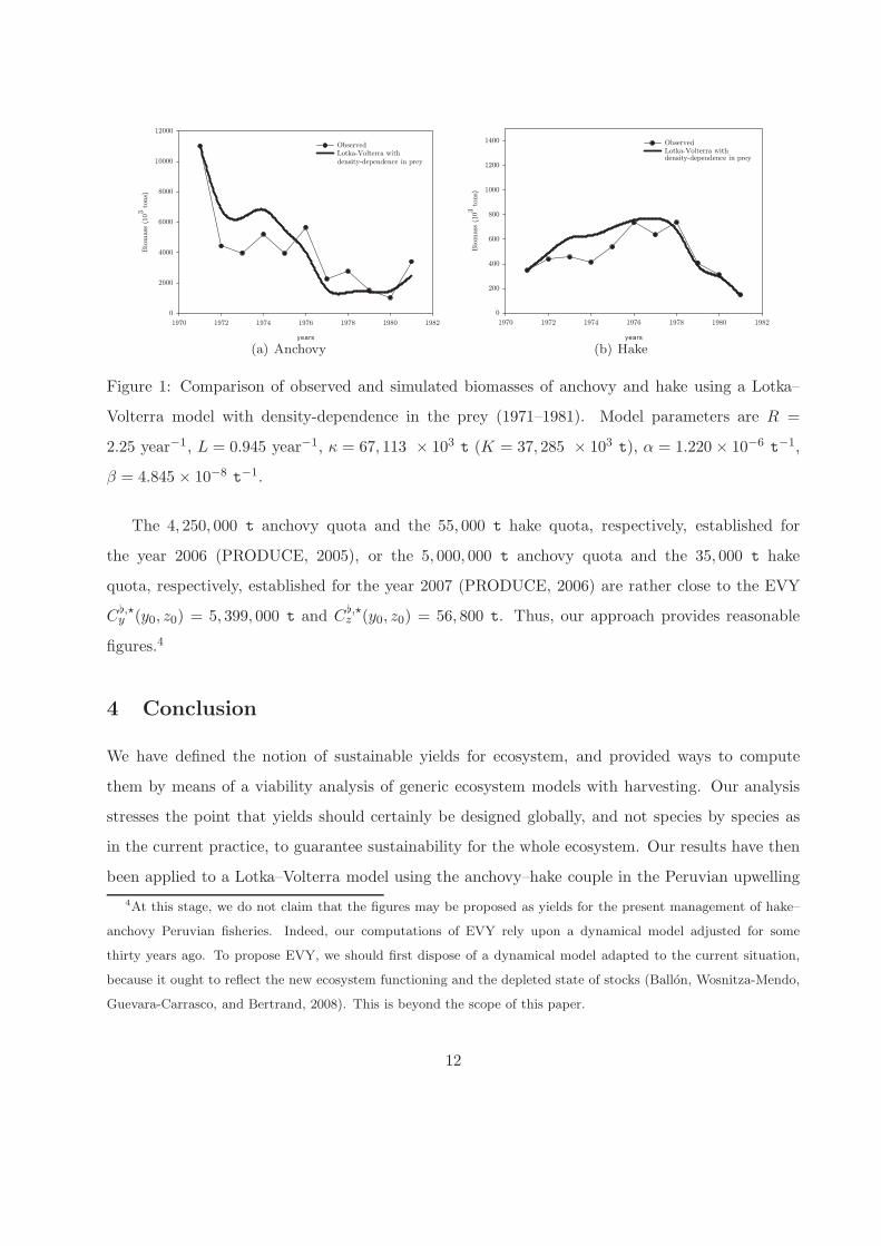
(a) Anchovy (b) Hake

Figure 1: Comparison of observed and simulated biomasses of anchovy and hake using a Lotka–

Volterra model with density-dependence in the prey (1971–1981). Model parameters are R =

2.25 year−1, L = 0.945 year−1, κ = 67, 113 × 103 t (K = 37, 285 × 103 t), α = 1.220 × 10−6t−1,

β = 4.845 × 10−8t−1.

The 4, 250, 000 t anchovy quota and the 55, 000 t hake quota, respectively, established for

the year 2006 (PRODUCE, 2005), or the 5, 000, 000 t anchovy quota and the 35, 000 t hake

quota, respectively, established for the year 2007 (PRODUCE, 2006) are rather close to the EVY

C♭,⋆y (y0, z0) = 5, 399, 000 t and C

♭,⋆z (y0, z0) = 56, 800 t. Thus, our approach provides reasonable

figures.4

4 Conclusion

We have defined the notion of sustainable yields for ecosystem, and provided ways to compute

them by means of a viability analysis of generic ecosystem models with harvesting. Our analysis

stresses the point that yields should certainly be designed globally, and not species by species as

in the current practice, to guarantee sustainability for the whole ecosystem. Our results have then

been applied to a Lotka–Volterra model using the anchovy–hake couple in the Peruvian upwelling

4At this stage, we do not claim that the figures may be proposed as yields for the present management of hake–

anchovy Peruvian fisheries. Indeed, our computations of EVY rely upon a dynamical model adjusted for some

thirty years ago. To propose EVY, we should first dispose of a dynamical model adapted to the current situation,

because it ought to reflect the new ecosystem functioning and the depleted state of stocks (Ballon, Wosnitza-Mendo,

Guevara-Carrasco, and Bertrand, 2008). This is beyond the scope of this paper.

12

ecosystem. Despite simplicity5 of the models considered, our approach has provided reasonable

figures and new insights: it may be a mean of designing sustainable yields from an ecosystem point

of view.

We now discuss the limits of the EVY concept, as presented in this paper: application to biomass

ecosystem models without age or spatial structure, no economic consideration, no uncertainties.

We stress that EVY is a flexible concept, and we hint at possible extensions to incorporate the

missing dimensions listed above.

The framework we propose is not restricted to two populations, each described by its global

biomass, but it may be adapted to several species, each described by a vector of abundances at

age, or by vectors of abundances at age for each patch in a spatial model, etc. Suppose that the

time evolution is given by a dynamical equation reflecting ecosystemic interactions and driven by

efforts or by catches. Suppose that minimal safety levels (reference points) are fixed for biological

indicators like spawning stock biomass, abundances at specific ages, etc. (such reference points for

biological indicators like spawning stock biomass are generally given by international bodies like

the ICES, or nationally). Ecosystem viable yields are minimal harvests for each species which can

be guaranteed for all times while respecting the above minimal safety levels for biological indicators

for all times too.

It is often objected with reason that the MSY concept is developed without any economic

consideration. As presented here, the EVY suffers the same criticism. However, the EVY concept is

flexible enough to incorporate some economic considerations. For instance, upper bounds for fishing

costs may be incorporated as constraints to be satisfied for all time, aside with minimal biomass

levels. In this sense, EVY will be guaranteed yields compatible with biological and economic

restrictions.

As presented here, the EVY framework supposes that no uncertainties affect the ecosystem

dynamics. Though we have the tools to tackle such an important issue (see stochastic viability

in (De Lara and Doyen, 2008; De Lara and Martinet, 2009; Doyen and De Lara, 2010)), we feel

that we have to go step by step. This paper introduces the EVY concept in the deterministic case,

5In addition to hake, there are other important predators of anchovy in the Peruvian upwelling ecosystem, such

as mackerel and horse mackerel, seabirds and pinnipeds, which were not considered. Also, anchovy has been an

important prey of hake, but other prey species have been found in the opportunistic diet of hake (Tam, Purca,

Duarte, Blaskovic, and Espinoza, 2006)

13

providing an extension of the MSY concept in two directions: from equilibrium to viability (more

robust), from monospecies to multispecies models. The extension to the uncertain case is currently

under investigation.

Thus, control and viability theory methods have allowed us to introduce ecosystem consider-

ations, such as multispecies and multiobjectives, and have contributed to integrate the long term

dynamics, which is generally not considered in conventional fishery management.

Acknowledgments. This paper was prepared within the MIFIMA (Mathematics, Informatics

and Fisheries Management) international research network; we thank CNRS, INRIA and the French

Ministry of Foreign Affairs for their funding and support through the regional cooperation program

STIC–AmSud. We thank the staff of the Peruvian Marine Research Institute (IMARPE), especially

Erich Diaz and Nathaly Vargas for discussions on anchovy and hake fisheries. We thank Sophie

Bertrand and Arnaud Bertrand from IRD at IMARPE for their insightful comments. We also

thank Yboon Garcia (IMCA-Peru and CMM-Chile) for a discussion on the ecosystem model case.

We are particularly indebted to the reviewer who, by his/her comments and questions, helped us

improve the presentation.

A Discrete–time viability

Let us consider a nonlinear control system described in discrete–time by the dynamic equation

x(t+ 1) = f(

x(t), u(t))

for all t ∈ N,

x(0) = x0 given,(16)

where the state variable x(t) belongs to the finite dimensional state space X = RnX, the control

variable u(t) is an element of the control set U = RnU while the dynamics f maps X× U into X.

A controller or a decision maker describes “acceptable configurations of the system” through a

set D ⊂ X× U termed the acceptable set

(

x(t), u(t))

∈ D for all t ∈ N , (17)

where D includes both system states and controls constraints.

14

The state constraints set V0 associated with D is obtained by projecting the acceptable set D

onto the state space X:

V0 := ProjX(D) = {x ∈ X | ∃u ∈ U , (x, u) ∈ D} . (18)

Viability is defined as the ability to choose, at each time step t ∈ N, a control u(t) ∈ U such that

the system configuration remains acceptable. More precisely, viability occurs when the following

set of initial states is not empty:

V(f,D) :=

x0 ∈ X

∣

∣

∣

∣

∣

∣

∃ (u(0), u(1), . . .) and (x(0), x(1), . . .)

satisfying (16) and (17)

. (19)

The set V(f,D) is called the viability kernel (Aubin, 1991) associated with the dynamics f and the

acceptable set D. By definition, we have V(f,D) ⊂ V0 = ProjX(D) but, in general, the inclusion is

strict. For a decision maker or control designer, knowing the viability kernel has practical interest

since it describes the initial states for which controls can be found that maintain the system in an

acceptable configuration forever. However, computing this kernel is not an easy task in general.

We now focus on some tools to achieve viability. A subset V is said to be weakly invariant for

the dynamics f in the acceptable set D, or a viability domain of f in D, if

∀x ∈ V , ∃u ∈ U , (x, u) ∈ D and f(x, u) ∈ V . (20)

That is, if one starts from V, an acceptable control may transfer the state in V. Moreover, according

to viability theory (Aubin, 1991), the viability kernel V(f,D) turns out to be the union of all viability

domains, or also the largest viability domain:

V(f,D) =⋃

{

V, V ⊂ V0, V viability domain for f in D

}

. (21)

Viable controls are those controls u ∈ U such that (x, u) ∈ D and f(x, u) ∈ V(f,D).

A major interest of such a property lies in the fact that any viability domain for the dynamics

f in the acceptable set D provides a lower approximation of the viability kernel. An upper approx-

imation Vk of the viability kernel is given by the so called viability kernel until time k associated

with f in D:

Vk :=

x0 ∈ X

∣

∣

∣

∣

∣

∣

∣

∣

∣

∃ (u(0), u(1), . . . , u(k)) and (x(0), x(1), . . . , x(k))

satisfying (16) for t = 0, . . . , k − 1

and (17) for t = 0, . . . , k

. (22)

15

We have

V(f,D) ⊂ Vk+1 ⊂ Vk ⊂ V0 = V0 for all k ∈ N . (23)

It may be seen by induction that the decreasing sequence of viability kernels until time k satisfies

V0 = V0 and Vk+1 = {x ∈ Vk | ∃u ∈ U , (x, u) ∈ D and f(x, u) ∈ Vk } . (24)

By (23), such an algorithm provides approximation from above of the viability kernel as follows:

V(f,D) ⊂⋂

k∈N

Vk = limk→+∞

↓Vk . (25)

Conditions ensuring that equality holds may be found in (Saint-Pierre, 1994). Notice that, when the

decreasing sequence (Vk)k∈N of viability kernels up to time k is stationary, its limit is the viability

kernel. Indeed, if Vk = Vk+1 for some k, then Vk is a viability domain by (24). Now, by (19),

V(f,D) is the largest of viability domains. As a consequence, Vk = V(f,D) since V(f,D) ⊂ Vk

by (23). We shall use this property in the following Sect. B.

B Viable control of generic nonlinear ecosystem models with har-

vesting

For a generic ecosystem model (1), we provide an explicit description of the viability kernel. Then,

we shall specify the results for predator–prey systems, in particular for discrete-time Lotka–Volterra

models.

The acceptable set D in (17) is defined by minimal biomass levels B♭y ≥ 0, B♭

z ≥ 0 and minimal

catch levels C♭y ≥ 0, C♭

z ≥ 0:

D = { (y, z, v, w) ∈ R4 | y ≥ B♭

y, z ≥ B♭z, vy ≥ C♭

y, wz ≥ C♭z } . (26)

B.1 Expression of the viability kernel

The following Proposition 5 gives an explicit description of the viability kernel, under some condi-

tions on the minimal levels.

Proposition 5 Assume that the function Ry : R3 → R is continuously decreasing in the control

v and satisfies limv→+∞Ry(y, z, v) ≤ 0, and that Rz : R3 → R is continuously decreasing in the

16

control variable w, and satisfies limw→+∞Rz(y, z, w) ≤ 0. If the minimal levels in (26) are such

that the following growth factors are greater than one

Ry(B♭y, B

♭z,

C♭y

B♭y

) ≥ 1 and Rz(B♭y, B

♭z,

C♭z

B♭z

) ≥ 1 , (27)

the viability kernel associated with the dynamics f in (1) and the acceptable set D in (26) is given

by

V(f,D) =

{

(y, z) | y ≥ B♭y, z ≥ B♭

z, yRy(y, z,C♭y

y) ≥ B♭

y, zRz(y, z,C♭z

z) ≥ B♭

z

}

. (28)

Proof. According to induction (24), we have:

V0 = { (y, z)∣

∣

∣y ≥ B♭

y, z ≥ B♭z },

V1 =

(y, z)

∣

∣

∣

∣

∣

∣

y ≥ B♭y, z ≥ B♭

z and, for some (v, w) ≥ 0,

vy ≥ C♭y , wz ≥ C♭

z , yRy(y, z, v) ≥ B♭y, zRz(y, z, w) ≥ B♭

z

=

{

(y, z)

∣

∣

∣

∣

∣

y ≥ B♭y, z ≥ B♭

z, yRy(y, z,C♭

y

y) ≥ B♭

y, zRz(y, z,C♭

z

z) ≥ B♭

z

}

because v 7→ Ry(y, z, v) and w 7→ Rz(y, z, w) are decreasing,

and thus we may select v =C♭

y

y, w =

C♭z

z.

Denoting y′ = yRy(y, z, v), z′ = zRz(y, z, w), we obtain,

V2 =

(y, z)

∣

∣

∣

∣

∣

∣

∣

∣

∣

y ≥ B♭y, z ≥ B♭

z and, for some (v, w) ≥ 0,

vy ≥ C♭y , wz ≥ C♭

z

y′ ≥ B♭y, y′Ry(y

′, z′,C♭

y

y′) ≥ B♭

y, z′ ≥ B♭z, z′Rz(y

′, z′,C♭

z

z′) ≥ B♭

z

.

We shall now make use of the property, recalled in Sect. A, that when the decreasing sequence (Vk)k∈N of

viability kernels up to time k is stationary, its limit is the viability kernel V(f,D). Hence, it suffices to show

that V1 ⊂ V2 to obtain that V(f,D) = V1. Let (y, z) ∈ V1, so that

y ≥ B♭y, z ≥ B♭

z and yRy(y, z,C♭

y

y) ≥ B♭

y, zRz(y, z,C♭

z

z) ≥ B♭

z .

Since Ry : R3 → R is continuously decreasing in the control variable, with limv→+∞ Ry(y, z, v) ≤ 0, and

since yRy(y, z,C♭

y

y) ≥ B♭

y, there exists a v ≥C♭

y

y(depending on y and z) such that y′ = yRy(y, z, v) = B♭

y.

The same holds for Rz : R3 → R and z′ = zRz(y, z, w) = B♭z . By (27), we deduce that

y′Ry(y′, z′,

C♭y

y′) = B♭

yRy(B♭y , B

♭z,

C♭y

B♭y

) ≥ B♭y and z′Rz(y

′, z′,C♭

z

z′) = B♭

zRz(B♭y , B

♭z,

C♭z

B♭z

) ≥ B♭z .

The inclusion V1 ⊂ V2 follows. 2

17

Corollary 6 Suppose that the assumptions of Proposition 2 are satisfied. Denoting

v(y, z) = max{v ≥C♭

y

y| yRy(y, z, v) = y♭} ,

w(y, z) = max{w ≥ C♭z

z| zRz(y, z, w) = z♭} ,

the set of viable controls is given by

UV(f,D)(y, z) =

(v,w)

∣

∣

∣

∣

∣

∣

v(y, z) ≥ v ≥C♭

y

y , w(y, z) ≥ w ≥ C♭zz ,

y′Ry(y′, z′,

C♭y

y′) ≥ y♭, z′Rz(y

′, z′,C♭

z

z′) ≥ z♭

,

where y′ = yRy(y, z, v), z′ = zRz(y, z, w).

B.2 Proof of Proposition 4

Proof. By (9), and the property that both Ry and Rz are decreasing in the control variable, the quantities (8)

exist.

Also since both Ry and Rz are decreasing in the control variable, we obtain that

Ry(B♭y, B

♭z ,

C♭,⋆y (y0, z0)

B♭y

) ≥ Ry(B♭y, B

♭z,

C♭,⋆y

B♭y

) = 1 and Rz(B♭y, B

♭z ,

C♭,⋆z (y0, z0)

B♭z

) ≥ Rz(B♭y, B

♭z,

C♭,⋆z

B♭z

) = 1 .

To end up, the above inequalities and the assumption that y0 ≥ B♭y and z0 ≥ B♭

z allow us to conclude, thanks

to Proposition 5, that (y0, z0) belongs to the viability kernel V(f,D) given in (28).

In other words, starting from the initial point (y(t0), z(t0)) = (y0, z0), there exists an appropriate har-

vesting path which can provide, for all time, at least the catches (8). 2

References

Jurgen Alheit and Miguel Niquen. Regime shifts in the Humboldt Current Ecosystem. Progress

in Oceanography, 60:201–222, 2004.

J-P. Aubin. Viability Theory. Birkhauser, Boston, 1991. 542 pp.

Michael Ballon, Claudia Wosnitza-Mendo, Renato Guevara-Carrasco, and Arnaud Bertrand. The

impact of overfishing and El Nino on the condition factor and reproductive success of Peruvian

hake, Merluccius gayi peruanus. Progress In Oceanography, 79(2-4):300 – 307, 2008.

C. Bene and L. Doyen. Sustainability of fisheries through marine reserves: a robust modeling

analysis. Journal of Environmental Management, 69(1):1–13, 2003.

18

C. Bene, L. Doyen, and D. Gabay. A viability analysis for a bio-economic model. Ecological

Economics, 36:385–396, 2001.

Arnaud Bertrand, Marceliano Segura, Mariano Gutierrez, and Luis Vasquez. From small-scale

habitat loopholes to decadal cycles: a habitat-based hypothesis explaining fluctuation in pelagic

fish populations off Peru. Fish and Fisheries, 5:296–316, 2004.

D. Bertsekas and I. Rhodes. On the minimax reachability of target sets and target tubes. Auto-

matica, 7:233–247, 1971.

Laetitia Chapel, Guillaume Deffuant, Sophie Martin, and Christian Mullon. Defining yield policies

in a viability approach. Ecological Modelling, 212(1-2):10 – 15, 2008.

David M. Checkley, Jurgen Alheit, Yoshioki Ooseki, and Claude Roy. Climate Change and Small

Pelagic Fish. Cambridge University Press, 2009.

C. W. Clark. Mathematical Bioeconomics. Wiley, New York, second edition, 1990.

F. H. Clarke, Y. S. Ledayev, R. J. Stern, and P. R. Wolenski. Qualitative properties of trajectories

of control systems: a survey. Journal of Dynamical Control Systems, 1:1–48, 1995.

M. De Lara and L. Doyen. Sustainable Management of Natural Resources. Mathematical Models

and Methods. Springer-Verlag, Berlin, 2008.

M. De Lara and V. Martinet. Multi-criteria dynamic decision under uncertainty: A stochastic via-

bility analysis and an application to sustainable fishery management. Mathematical Biosciences,

217(2):118–124, February 2009.

M. De Lara, L. Doyen, T. Guilbaud, and M.-J. Rochet. Is a management framework based on

spawning-stock biomass indicators sustainable? A viability approach. ICES J. Mar. Sci., 64(4):

761–767, 2007.

L. Doyen and M. De Lara. Stochastic viability and dynamic programming. Systems and Control

Letters, 59(10):629–634, October 2010.

K. Eisenack, J. Sheffran, and J. Kropp. The viability analysis of management frameworks for

fisheries. Environmental Modeling and Assessment, 11(1):69–79, February 2006.

19

FAO. Indicators for sustainable development of marine capture fisheries. FAO Technical Guidelines

for Responsible Fisheries 8, FAO, 1999. 68 pp.

S. Garcia, A. Zerbi, C. Aliaume, T. Do Chi, and G. Lasserre. The ecosystem approach to fisheries.

Issues, terminology, principles, institutional foundations, implementation and outlook. FAO

Fisheries Technical Paper, 443(71), 2003.

C. Hall. An assessment of several of the historically most influential theoretical models used in

ecology and of the data provided in their support. Ecological Modelling, 43(1-2):5–31, 1988.

Anne B. Hollowed, Nicholas Bax, Richard Beamish, Jeremy Collie, Michael Fogarty, Patricia Liv-

ingston, John Pope, and Jake C. Rice. Are multispecies models an improvement on single-species

models for measuring fishing impacts on marine ecosystems? ICES J. Mar. Sci., 57(3):707–719,

2000.

ICES. Report of the ICES advisory committee on fishery management and advisory committee on

ecosystems, 2004. ICES Advice, 1, ICES, 2004. 1544 pp.

IMARPE. Trabajos expuestos en el taller internacional sobre la anchoveta peruana (TIAP), 9-12

Mayo 2000. Bol. Inst. Mar Peru, 19:1–2, 2000.

IMARPE. Report of the first session of the international panel of experts for assessment of Peruvian

hake population. March 2003. Bol. Inst. Mar Peru, 21:33–78, 2004.

Stephen L. Katz, Richard Zabel, Chris Harvey, Thomas Good, and Phillip Levin. Ecologically

sustainable yield. American Scientist, 91(2):150, March-April 2003.

P. A. Larkin. An Epitaph for the Concept of Maximum Sustained Yield. Transactions of the

American Fisheries Society, 106(1):1–11, January 1977.

C. Mullon, P. Cury, and L. Shannon. Viability model of trophic interactions in marine ecosystems.

Natural Resource Modeling, 17:27–58, 2004.

J. D. Murray. Mathematical Biology. Springer-Verlag, Berlin, third edition, 2002.

Daniel Pauly and Marıa Lourdes Palomares. New estimates of monthly biomass, recruitment and

related statistics of anchoveta (Engraulis ringens) off Peru (4-14 ◦S), 1953-1985, pages 189–206.

18. ICLARM Conference Proceedings, 1989.

20

PRODUCE. Establecen regimen provisional de pesca del recurso merluza correspondiente al ano

2006. El Peruano, page 307804, 30 de diciembre 2005. RM-356-2005-PRODUCE.

PRODUCE. Establecen regimen provisional de pesca del recurso merluza correspondiente al ano

2007. El Peruano, page 335485, 27 de diciembre 2006. RM-357-2006-PRODUCE.

A. Rapaport, J.-P. Terreaux, and L. Doyen. Sustainable management of renewable resource: a

viability approach. Mathematics and Computer Modeling, 43(5-6):466–484, March 2006.

P. Saint-Pierre. Approximation of viability kernel. Applied Mathematics and Optimization, 29:

187–209, 1994.

M. B. Schaefer. Some aspects of the dynamics of populations important to the management of

commercial marine fisheries. Bulletin of the Inter-American tropical tuna commission, 1:25–56,

1954.

Chin-Hwa Sun, Fu-Sung Chiang, Te-Shi Liu, and Ching-Cheng Chang. A welfare analysis of El Nino

forecasts in the international trade of fish meal - an application of stochastic spatial equilibrium

model. 2001 Annual meeting, August 5-8, Chicago, IL 20770, American Agricultural Economics

Association (New Name 2008: Agricultural and Applied Economics Association), 2001.

J. Tam, S. Purca, L. O. Duarte, V. Blaskovic, and P. Espinoza. Changes in the diet of hake

associated with El Nino 1997-1998 in the Northern Humboldt Current ecosystem. Advances in

Geosciences., 6:63–67, 2006.

21