MGS8020 Analyze.ppt/Apr 2, 2015/Page 1 Georgia State University - Confidential MGS 8020 Business...
49
MGS8020 Analyze.ppt/Apr 2, 2015/Page 1 Georgia State University - Confidential MGS 8020 Business Intelligence Analyze Apr 2, 2015
-
Upload
alicia-blankenship -
Category
Documents
-
view
217 -
download
0
Transcript of MGS8020 Analyze.ppt/Apr 2, 2015/Page 1 Georgia State University - Confidential MGS 8020 Business...
MGS8020 Analyze.ppt/Apr 2, 2015/Page 1Georgia State University - Confidential
MGS 8020
Business Intelligence
Analyze
Apr 2, 2015
MGS8020 Analyze.ppt/Apr 2, 2015/Page 2Georgia State University - Confidential
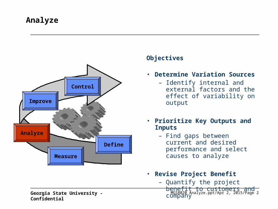
Analyze
Measure
Control
Analyze
Improve
Define
Objectives
• Determine Variation Sources – Identify internal and external
factors and the effect of variability on output
• Prioritize Key Outputs and Inputs– Find gaps between current and
desired performance and select causes to analyze
• Revise Project Benefit – Quantify the project benefit to
customers and company
MGS8020 Analyze.ppt/Apr 2, 2015/Page 3Georgia State University - Confidential
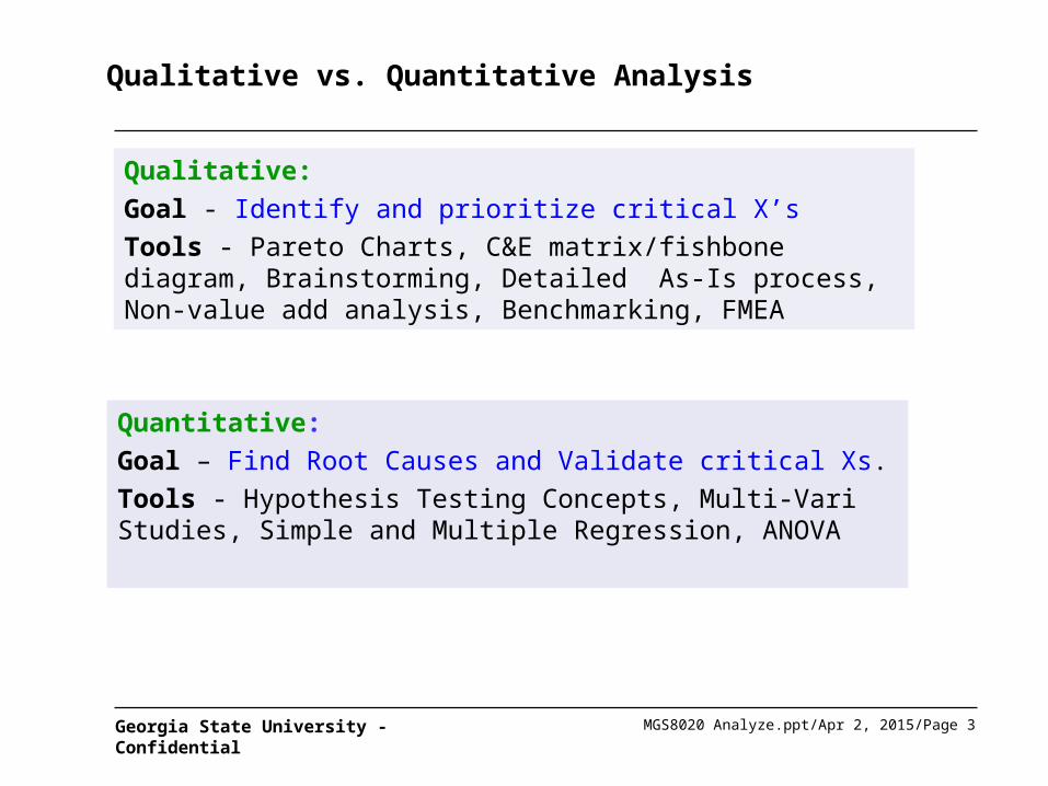
Qualitative vs. Quantitative Analysis
Qualitative:
Goal - Identify and prioritize critical X’s
Tools - Pareto Charts, C&E matrix/fishbone diagram, Brainstorming, Detailed As-Is process, Non-value add analysis, Benchmarking, FMEA
Quantitative:
Goal – Find Root Causes and Validate critical Xs.
Tools - Hypothesis Testing Concepts, Multi-Vari Studies, Simple and Multiple Regression, ANOVA
MGS8020 Analyze.ppt/Apr 2, 2015/Page 4Georgia State University - Confidential
Agenda
1. Process Analysis
2. Qualitative Analysis
3. Quantitative Analysis
MGS8020 Analyze.ppt/Apr 2, 2015/Page 5Georgia State University - Confidential
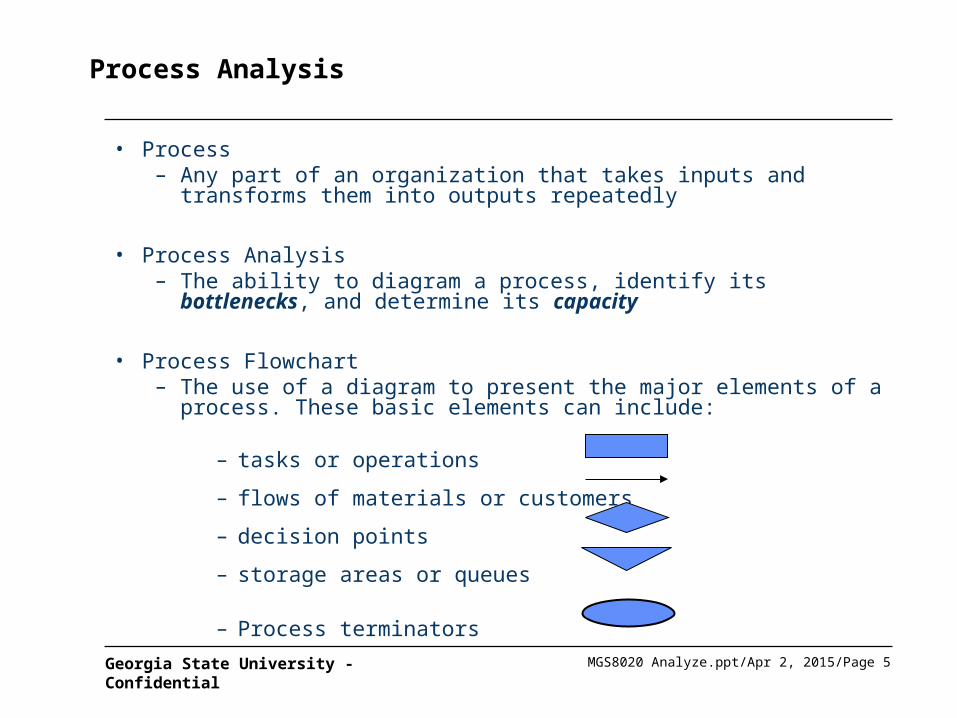
Process Analysis
• Process– Any part of an organization that takes inputs and transforms them into
outputs repeatedly
• Process Analysis – The ability to diagram a process, identify its bottlenecks, and determine its
capacity
• Process Flowchart– The use of a diagram to present the major elements of a process. These
basic elements can include:
– tasks or operations
– flows of materials or customers
– decision points
– storage areas or queues
– Process terminators
MGS8020 Analyze.ppt/Apr 2, 2015/Page 6Georgia State University - Confidential
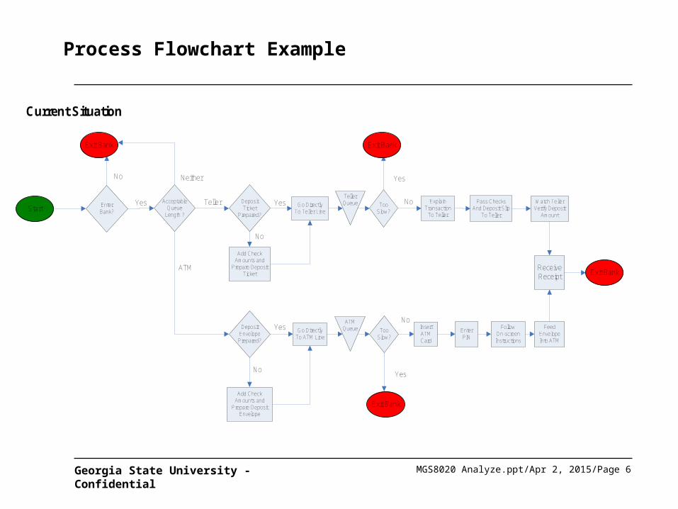
Process Flowchart Example
Enter Bank?
No
Deposit Ticket
Prepared?
Yes Go Directly To Teller Line
Explain Transaction
To Teller
Watch Teller Verify Deposit
Amount
Receive Receipt
Acceptable Queue
Length ?
Yes
No
Add Check Amounts and
Prepare Deposit Ticket
Teller
ATM
Neither
Deposit Envelope Prepared?
Add Check Amounts and
Prepare Deposit Envelope
No
Go Directly To ATM Line
Insert ATM Card
Enter PIN
Teller Queue
ATM QueueYes
Too Slow?
Too Slow?
No
No
Yes
Yes
Follow On-screen Instructions
Feed Envelope Into ATM
Pass Checks And Deposit Slip
To Teller
Current Situation
Exit Bank Exit Bank
Exit Bank
Exit Bank
Start
MGS8020 Analyze.ppt/Apr 2, 2015/Page 7Georgia State University - Confidential
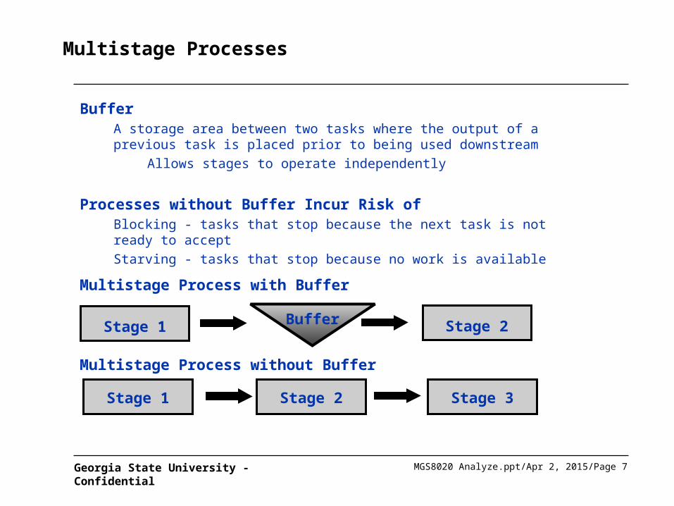
Multistage Processes
BufferA storage area between two tasks where the output of a previous task is placed prior to being used downstream
Allows stages to operate independently
Processes without Buffer Incur Risk ofBlocking - tasks that stop because the next task is not ready to accept
Starving - tasks that stop because no work is available
Stage 1 Stage 2 Stage 3
Multistage Process with Buffer
Stage 1 Stage 2Buffer
Multistage Process without Buffer
MGS8020 Analyze.ppt/Apr 2, 2015/Page 8Georgia State University - Confidential
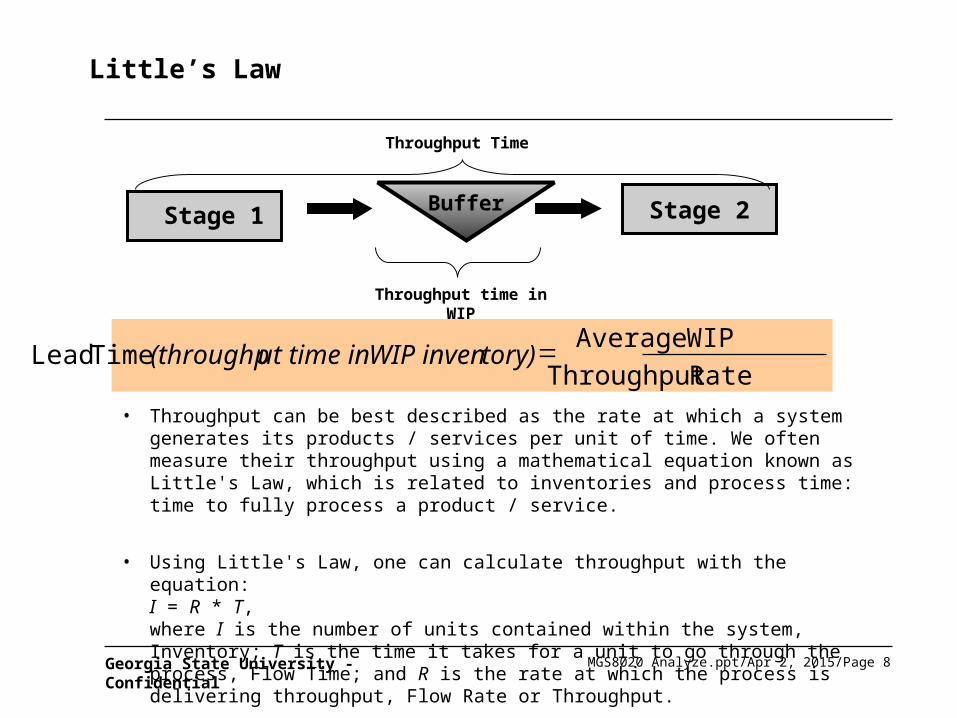
Little’s Law
Stage 1 Stage 2Buffer
Throughput Time
Throughput time in WIP
Rate Throughput
WIPAverage Time Lead tory) WIP invenut time in (throughp
• Throughput can be best described as the rate at which a system generates its products / services per unit of time. We often measure their throughput using a mathematical equation known as Little's Law, which is related to inventories and process time: time to fully process a product / service.
• Using Little's Law, one can calculate throughput with the equation:I = R * T,where I is the number of units contained within the system, Inventory; T is the time it takes for a unit to go through the process, Flow Time; and R is the rate at which the process is delivering throughput, Flow Rate or Throughput.
MGS8020 Analyze.ppt/Apr 2, 2015/Page 9Georgia State University - Confidential
Process Analysis with Buffers
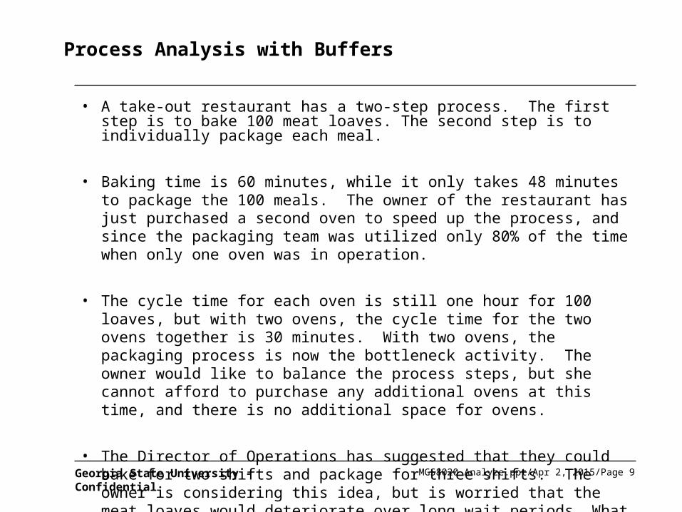
• A take-out restaurant has a two-step process. The first step is to bake 100 meat loaves. The second step is to individually package each meal.
• Baking time is 60 minutes, while it only takes 48 minutes to package the 100 meals. The owner of the restaurant has just purchased a second oven to speed up the process, and since the packaging team was utilized only 80% of the time when only one oven was in operation.
• The cycle time for each oven is still one hour for 100 loaves, but with two ovens, the cycle time for the two ovens together is 30 minutes. With two ovens, the packaging process is now the bottleneck activity. The owner would like to balance the process steps, but she cannot afford to purchase any additional ovens at this time, and there is no additional space for ovens.
• The Director of Operations has suggested that they could bake for two shifts and package for three shifts. The owner is considering this idea, but is worried that the meat loaves would deteriorate over long wait periods. What do you think?
MGS8020 Analyze.ppt/Apr 2, 2015/Page 10Georgia State University - Confidential
Process Analysis with Buffers
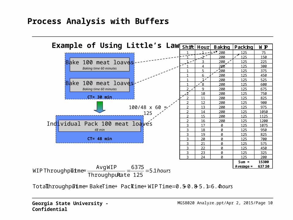
Example of Using Little’s Law
Individual Pack 100 meat loaves48 min
Bake 100 meat loavesBaking time 60 minutes
Bake 100 meat loavesBaking time 60 minutes
CT= 30 min
CT= 48 min
Shift Hour Baking Packing WIP1 1 200 125 751 2 200 125 1501 3 200 125 2251 4 200 125 3001 5 200 125 3751 6 200 125 4501 7 200 125 5251 8 200 125 6002 9 200 125 6752 10 200 125 7502 11 200 125 8252 12 200 125 9002 13 200 125 9752 14 200 125 10502 15 200 125 11252 16 200 125 12003 17 0 125 10753 18 0 125 9503 19 0 125 8253 20 0 125 7003 21 0 125 5753 22 0 125 4503 23 0 125 3253 24 0 125 200
Sum = 15300Average = 637.50
hours 1.5125
5.637
RateThroughput
WIP Avg = Time Throughput WIP
hours 6.45.10.80.5 Time WIP + Time Pack + Time Bake= Time Throughput Total
100/48 x 60 = 125
MGS8020 Analyze.ppt/Apr 2, 2015/Page 11Georgia State University - Confidential
Agenda
1. Process Analysis
2. Qualitative Analysis
3. Quantitative Analysis
MGS8020 Analyze.ppt/Apr 2, 2015/Page 12Georgia State University - Confidential
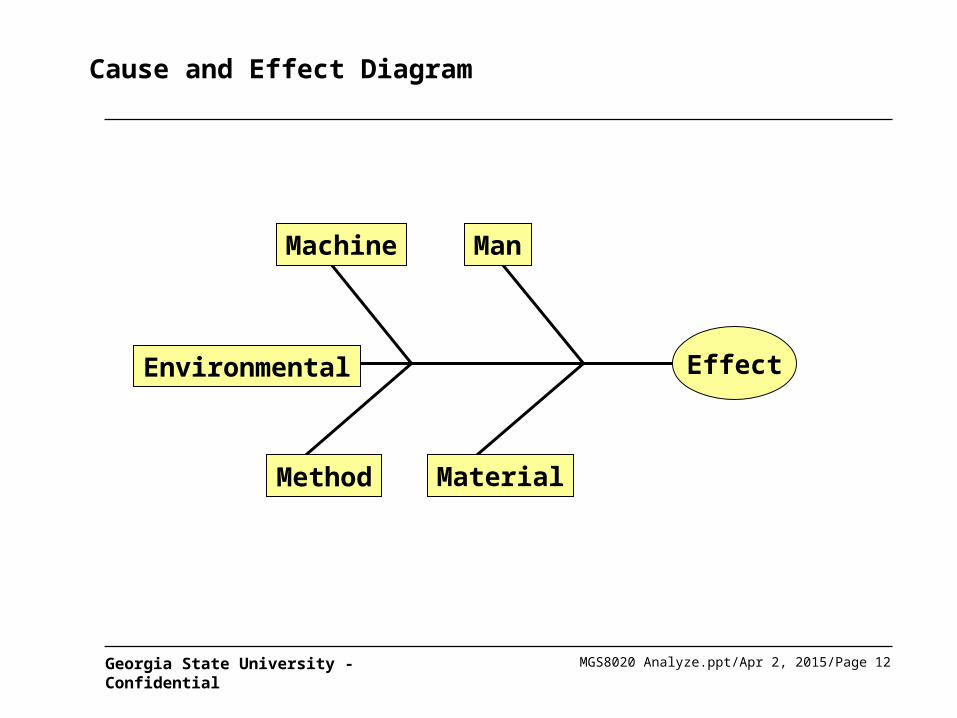
Cause and Effect Diagram
MaterialMethod
Environmental
ManMachine
Effect
MGS8020 Analyze.ppt/Apr 2, 2015/Page 13Georgia State University - Confidential
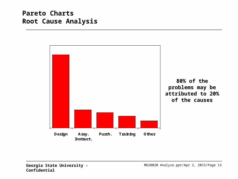
Pareto ChartsRoot Cause Analysis
Design Assy.Instruct.
Purch. Training Other
80% of theproblems may beattributed to 20%
of the causes
MGS8020 Analyze.ppt/Apr 2, 2015/Page 14Georgia State University - Confidential
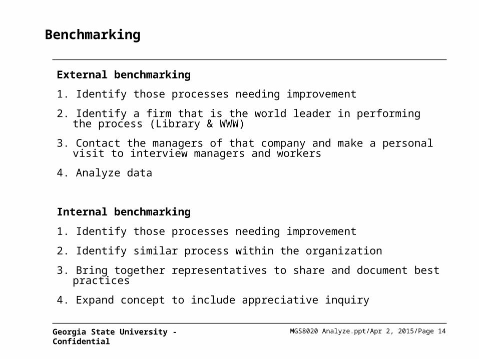
Benchmarking
External benchmarking
1. Identify those processes needing improvement
2. Identify a firm that is the world leader in performing the process (Library & WWW)
3. Contact the managers of that company and make a personal visit to interview managers and workers
4. Analyze data
Internal benchmarking
1. Identify those processes needing improvement
2. Identify similar process within the organization
3. Bring together representatives to share and document best practices
4. Expand concept to include appreciative inquiry
MGS8020 Analyze.ppt/Apr 2, 2015/Page 15Georgia State University - Confidential
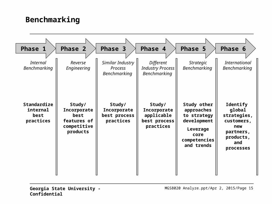
Benchmarking
Phase 1
Internal Benchmarking
Standardize internal best
practices
Phase 2
Reverse Engineering
Study/ Incorporate
best features of competitive
products
Phase 3
Similar Industry Process
Benchmarking
Study/ Incorporate
best process practices
Phase 4
Different Industry Process Benchmarking
Study/ Incorporate
applicable best process
practices
Phase 5
Strategic Benchmarking
Study other approaches to
strategy development
Leverage core competencies
and trends
Phase 6
International Benchmarking
Identify global strategies,
customers, new partners,
products, and processes
MGS8020 Analyze.ppt/Apr 2, 2015/Page 16Georgia State University - Confidential
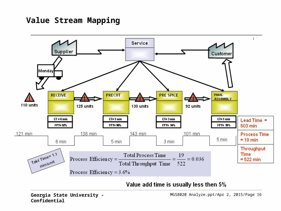
Value Stream Mapping
MGS8020 Analyze.ppt/Apr 2, 2015/Page 17Georgia State University - Confidential
Agenda
1. Process Analysis
2. Qualitative Analysis
3. Quantitative Analysis
MGS8020 Analyze.ppt/Apr 2, 2015/Page 18Georgia State University - Confidential
Agenda
Statistical Significance
MinitabOverview of
the Regression
MGS8020 Analyze.ppt/Apr 2, 2015/Page 19Georgia State University - Confidential
What is the Regression Analysis?
• The regression procedure is used when you are interested in describing the linear relationship between the independent variables and a dependent variable.
• A line in a two dimensional or two-variable space is defined by the equation Y=a+b*X
• In full text: the Y variable can be expressed in terms of a constant (a) and a slope (b) times the X variable.
• The constant is also referred to as the intercept, and the slope as the regression coefficient or B coefficient.
• For example, GPA may best be predicted as 1+.02*IQ. Thus, knowing that a student has an IQ of 130 would lead us to predict that her GPA would be 3.6 (since, 1+.02*130=3.6).
MGS8020 Analyze.ppt/Apr 2, 2015/Page 20Georgia State University - Confidential
What is the Regression Analysis?
• In the multivariate case, when there is more than one independent variable, the regression line cannot be visualized in the two dimensional space, but can be computed just as easily.
• For example, if in addition to IQ we had additional predictors of achievement (e.g., Motivation, Self- discipline) we could construct a linear equation containing all those variables. In general then, multiple regression procedures will estimate a linear equation of the form:
Y = a + b1*X1 + b2*X2 + ... + bp*Xp
MGS8020 Analyze.ppt/Apr 2, 2015/Page 21Georgia State University - Confidential
1) Predicted and Residual Scores
• The regression line expresses the best prediction of the dependent variable (Y), given the independent variables (X).
• However, nature is rarely (if ever) perfectly predictable, and usually there is substantial variation of the observed points around the fitted regression line (as in the scatterplot shown earlier). The deviation of a particular point from the regression line (its predicted value) is called the residual value.
MGS8020 Analyze.ppt/Apr 2, 2015/Page 22Georgia State University - Confidential
2) Residual Variance and R-square
• The smaller the variability of the residual values around the regression line relative to the overall variability, the better is our prediction.
• For example, if there is no relationship between the X and Y variables, then the ratio of the residual variability of the Y variable to the original variance is equal to 1.0. If X and Y are perfectly related then there is no residual variance and the ratio of variance would be 0.0. In most cases, the ratio would fall somewhere between these extremes, that is, between 0.0 and 1.0.
• 1.0 minus this ratio is referred to as R-square or the coefficient of determination. This value is immediately interpretable in the following manner. If we have an R-square of 0.4 then we know that the variability of the Y values around the regression line is 1-0.4 times the original variance; in other words we have explained 40% of the original variability, and are left with 60% residual variability.
• Ideally, we would like to explain most if not all of the original variability. The R-square value is an indicator of how well the model fits the data (e.g., an R-square close to 1.0 indicates that we have accounted for almost all of the variability with the variables specified in the model).
MGS8020 Analyze.ppt/Apr 2, 2015/Page 23Georgia State University - Confidential
2) R-square
• A mathematical term describing how much variation is being explained by the X.
• R-square = SSR / SST• SSR – SS (Regression)• SST – SS (Total)
MGS8020 Analyze.ppt/Apr 2, 2015/Page 24Georgia State University - Confidential
3) Adjusted R-square
• Adjusted R-square is the adjusted value for R-square will be equal or smaller than the regular R-square. The adjusted R-square adjusts for a bias in R-square.
• R-square tends to over estimate the variance accounted for compared to an estimate that would be obtained from the population. There are two reasons for the overestimate, a large number of predictors and a small sample size. So, with a small sample and with few predictors, adjusted R-square should be very similar the R-square value. Researchers and statisticians differ on whether to use the adjusted R-square. It is probably a good idea to look at it to see how much your R-square might be inflated, especially with a small sample and many predictors.
• Adjusted R-square = 1 – [MSR / (SST/(n – 1))]• MSR – MS (Regression)• SST – SS (Total)
MGS8020 Analyze.ppt/Apr 2, 2015/Page 25Georgia State University - Confidential
4) Coefficient R (Multiple R)
• Customarily, the degree to which two or more predictors (independent or X variables) are related to the dependent (Y) variable is expressed in the correlation coefficient R, which is the square root of R-square. In multiple regression, R can assume values between 0 and 1.
• To interpret the direction of the relationship between variables, one looks at the signs (plus or minus) of the regression or B coefficients. If a B coefficient is positive, then the relationship of this variable with the dependent variable is positive (e.g., the greater the IQ the better the grade point average); if the B coefficient is negative then the relationship is negative (e.g., the lower the class size the better the average test scores). Of course, if the B coefficient is equal to 0 then there is no relationship between the variables.
MGS8020 Analyze.ppt/Apr 2, 2015/Page 26Georgia State University - Confidential
5) ANOVA
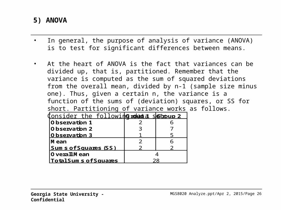
• In general, the purpose of analysis of variance (ANOVA) is to test for significant differences between means.
• At the heart of ANOVA is the fact that variances can be divided up, that is, partitioned. Remember that the variance is computed as the sum of squared deviations from the overall mean, divided by n-1 (sample size minus one). Thus, given a certain n, the variance is a function of the sums of (deviation) squares, or SS for short. Partitioning of variance works as follows. Consider the following data set:
Group 1 Group 2Observation 1 2 6Observation 2 3 7Observation 3 1 5Mean 2 6Sums of Squares (SS) 2 2Overall MeanTotal Sums of Squares
428
MGS8020 Analyze.ppt/Apr 2, 2015/Page 27Georgia State University - Confidential
6) Degree of Freedom (df)
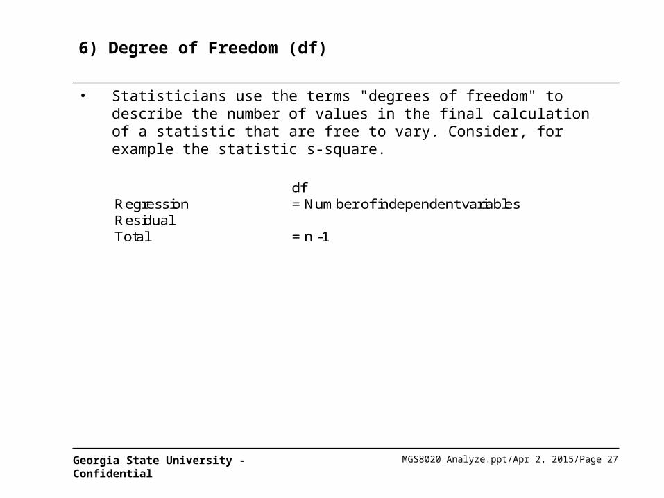
• Statisticians use the terms "degrees of freedom" to describe the number of values in the final calculation of a statistic that are free to vary. Consider, for example the statistic s-square.
dfRegression = Number of independent variablesResidualTotal = n -1
MGS8020 Analyze.ppt/Apr 2, 2015/Page 28Georgia State University - Confidential
7) S square & Sums of (deviation) squares
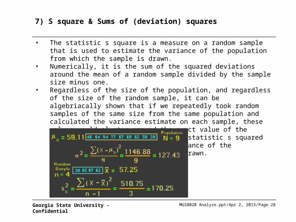
• The statistic s square is a measure on a random sample that is used to estimate the variance of the population from which the sample is drawn.
• Numerically, it is the sum of the squared deviations around the mean of a random sample divided by the sample size minus one.
• Regardless of the size of the population, and regardless of the size of the random sample, it can be algebriacally shown that if we repeatedly took random samples of the same size from the same population and calculated the variance estimate on each sample, these values would cluster around the exact value of the population variance. In short, the statistic s squared is an unbiased estimate of the variance of the population from which a sample is drawn.
MGS8020 Analyze.ppt/Apr 2, 2015/Page 29Georgia State University - Confidential
7) S square & Sums of (deviation) squares
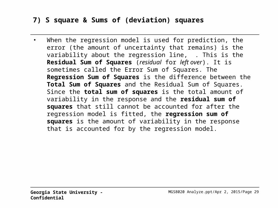
• When the regression model is used for prediction, the error (the amount of uncertainty that remains) is the variability about the regression line, . This is the Residual Sum of Squares (residual for left over). It is sometimes called the Error Sum of Squares. The Regression Sum of Squares is the difference between the Total Sum of Squares and the Residual Sum of Squares. Since the total sum of squares is the total amount of variability in the response and the residual sum of squares that still cannot be accounted for after the regression model is fitted, the regression sum of squares is the amount of variability in the response that is accounted for by the regression model.
MGS8020 Analyze.ppt/Apr 2, 2015/Page 30Georgia State University - Confidential
8) Mean Square Error
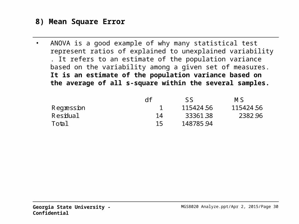
• ANOVA is a good example of why many statistical test represent ratios of explained to unexplained variability . It refers to an estimate of the population variance based on the variability among a given set of measures. It is an estimate of the population variance based on the average of all s-square within the several samples.
df SS MSRegression 1 115424.56 115424.56Residual 14 33361.38 2382.96Total 15 148785.94
MGS8020 Analyze.ppt/Apr 2, 2015/Page 31Georgia State University - Confidential
Agenda
Statistical Significance
MinitabOverview of
the Regression
MGS8020 Analyze.ppt/Apr 2, 2015/Page 32Georgia State University - Confidential
1) What is "statistical significance" (p-value)
• The statistical significance of a result is the probability that the observed relationship (e.g., between variables) or a difference (e.g., between means) in a sample occurred by pure chance ("luck of the draw"), and that in the population from which the sample was drawn, no such relationship or differences exist. Using less technical terms, one could say that the statistical significance of a result tells us something about the degree to which the result is "true" (in the sense of being "representative of the population").
• More technically, the value of the p-value represents a decreasing index of the reliability of a result (see Brownlee, 1960). The higher the p-value, the less we can believe that the observed relation between variables in the sample is a reliable indicator of the relation between the respective variables in the population.
• Specifically, the p-value represents the probability of error that is involved in accepting our observed result as valid, that is, as "representative of the population."
MGS8020 Analyze.ppt/Apr 2, 2015/Page 33Georgia State University - Confidential
1) What is "statistical significance" (p-value)
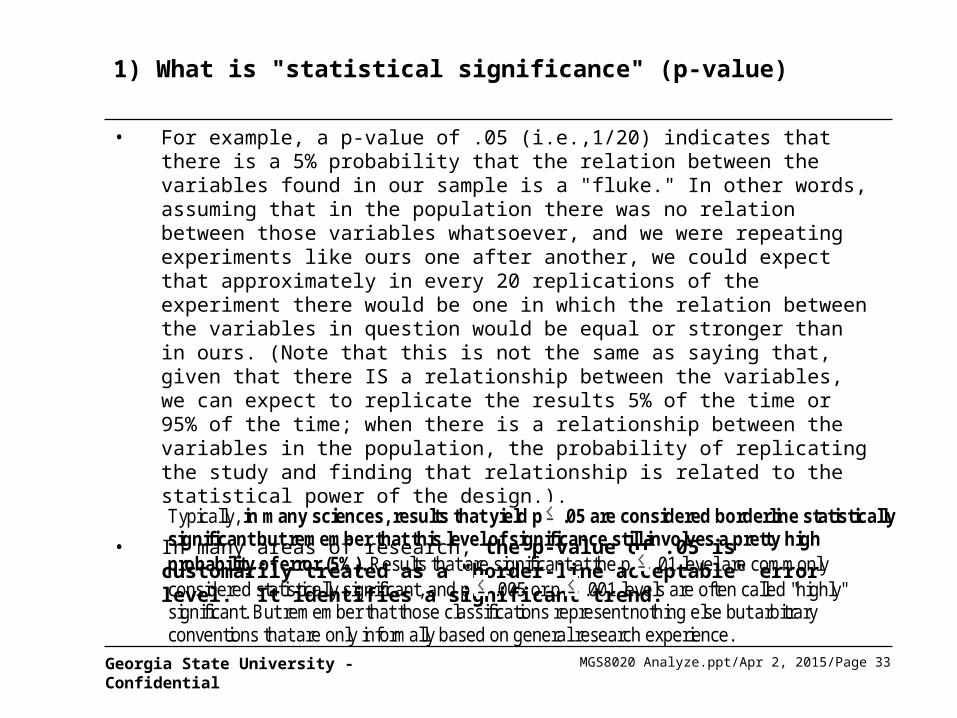
• For example, a p-value of .05 (i.e.,1/20) indicates that there is a 5% probability that the relation between the variables found in our sample is a "fluke." In other words, assuming that in the population there was no relation between those variables whatsoever, and we were repeating experiments like ours one after another, we could expect that approximately in every 20 replications of the experiment there would be one in which the relation between the variables in question would be equal or stronger than in ours. (Note that this is not the same as saying that, given that there IS a relationship between the variables, we can expect to replicate the results 5% of the time or 95% of the time; when there is a relationship between the variables in the population, the probability of replicating the study and finding that relationship is related to the statistical power of the design.).
• In many areas of research, the p-value of .05 is customarily treated as a "border-line acceptable" error level. It identifies a significant trend.
• fTypically, in many sciences, results that yield p .05 are considered borderline statistically significant but remember that this level of significance still involves a pretty high probability of error (5%). Results that are significant at the p .01 level are commonly considered statistically significant, and p .005 or p .001 levels are often called "highly" significant. But remember that those classifications represent nothing else but arbitrary conventions that are only informally based on general research experience.
MGS8020 Analyze.ppt/Apr 2, 2015/Page 34Georgia State University - Confidential
2) What is "statistical significance" (F-test & t-test)
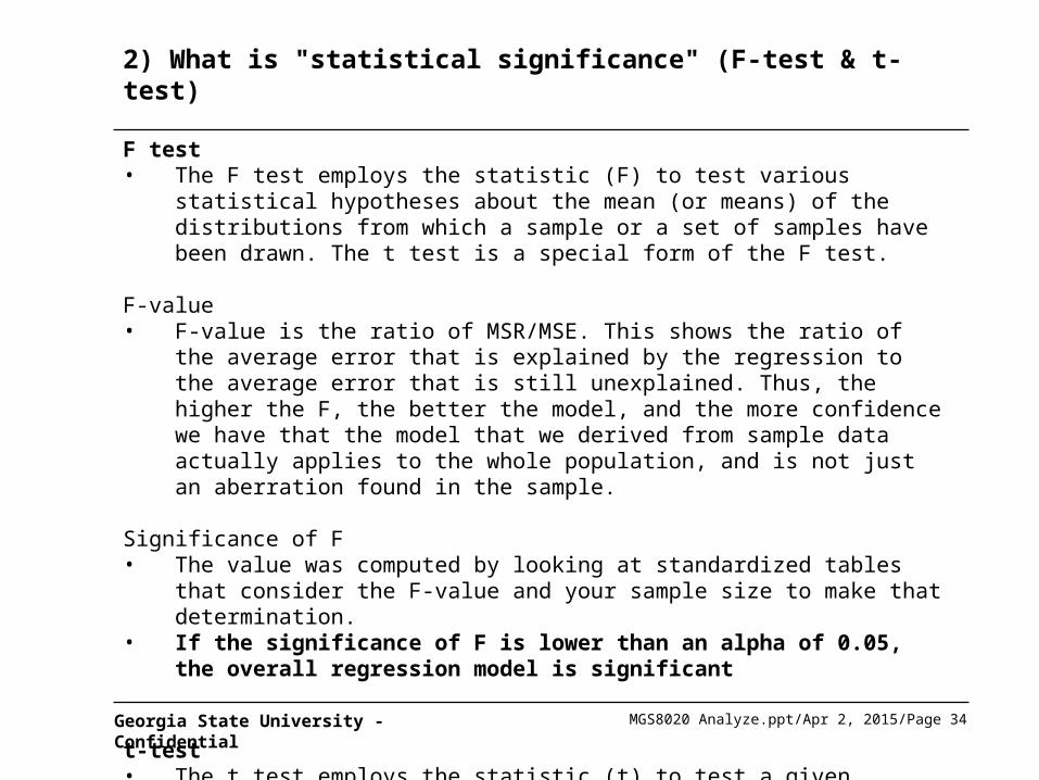
F test• The F test employs the statistic (F) to test various statistical hypotheses about
the mean (or means) of the distributions from which a sample or a set of samples have been drawn. The t test is a special form of the F test.
F-value• F-value is the ratio of MSR/MSE. This shows the ratio of the average error that
is explained by the regression to the average error that is still unexplained. Thus, the higher the F, the better the model, and the more confidence we have that the model that we derived from sample data actually applies to the whole population, and is not just an aberration found in the sample.
Significance of F • The value was computed by looking at standardized tables that consider the F-
value and your sample size to make that determination.• If the significance of F is lower than an alpha of 0.05, the overall regression
model is significant
t-test• The t test employs the statistic (t) to test a given statistical hypothesis about the
mean of a population (or about the means of two populations).
MGS8020 Analyze.ppt/Apr 2, 2015/Page 35Georgia State University - Confidential
Agenda
MinitabStatistical Significance
Overview of the
Regression
MGS8020 Analyze.ppt/Apr 2, 2015/Page 36Georgia State University - Confidential
Scatter Plot
MGS8020 Analyze.ppt/Apr 2, 2015/Page 37Georgia State University - Confidential
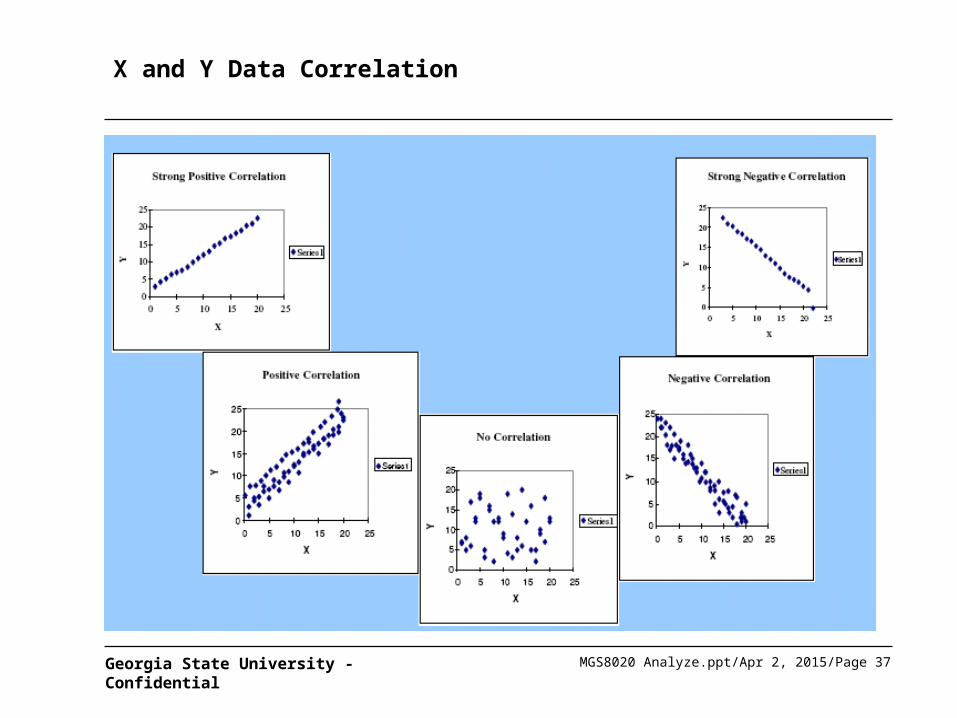
X and Y Data Correlation
MGS8020 Analyze.ppt/Apr 2, 2015/Page 38Georgia State University - Confidential
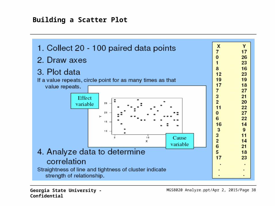
Building a Scatter Plot
MGS8020 Analyze.ppt/Apr 2, 2015/Page 39Georgia State University - Confidential
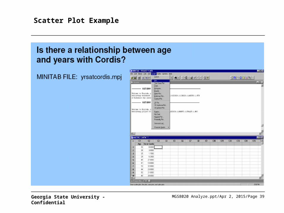
Scatter Plot Example
MGS8020 Analyze.ppt/Apr 2, 2015/Page 40Georgia State University - Confidential
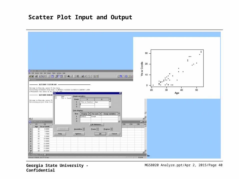
Scatter Plot Input and Output
MGS8020 Analyze.ppt/Apr 2, 2015/Page 41Georgia State University - Confidential
Simple Linear Regression
Regression analysis is a statistical technique1. Used to model and investigate the relationship between two or more
variables2. The model is often used for prediction
Regression is a hypothesis testHa: The model is a significant predictor of the response.
May be used to analyze relationships between the “Xs,” or between “Y” and “X.”
Regression is a powerful tool, but can never replace engineering or manufacturing process knowledge about trends.
MGS8020 Analyze.ppt/Apr 2, 2015/Page 42Georgia State University - Confidential
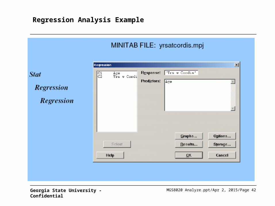
Regression Analysis Example
MGS8020 Analyze.ppt/Apr 2, 2015/Page 43Georgia State University - Confidential
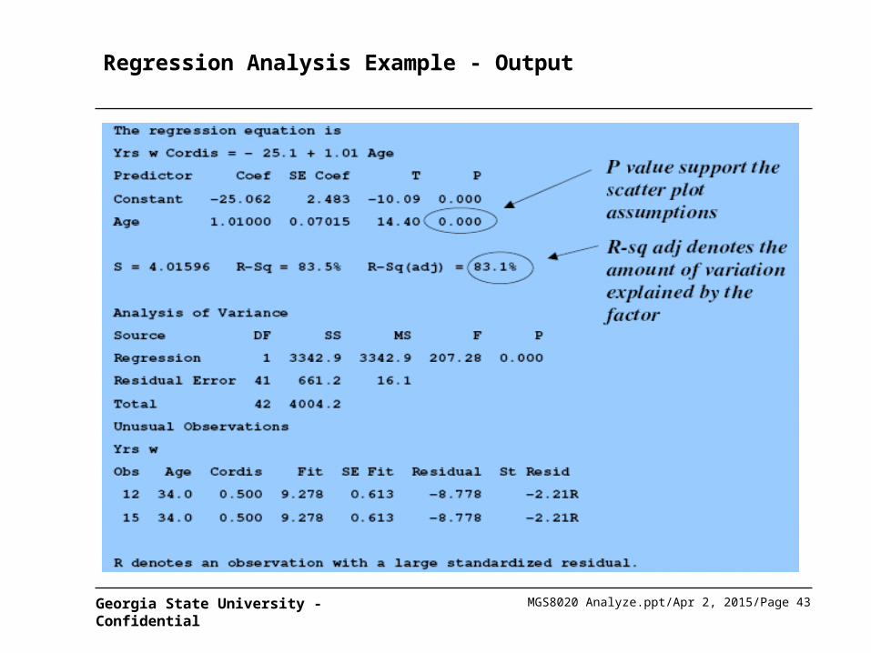
Regression Analysis Example - Output
MGS8020 Analyze.ppt/Apr 2, 2015/Page 44Georgia State University - Confidential
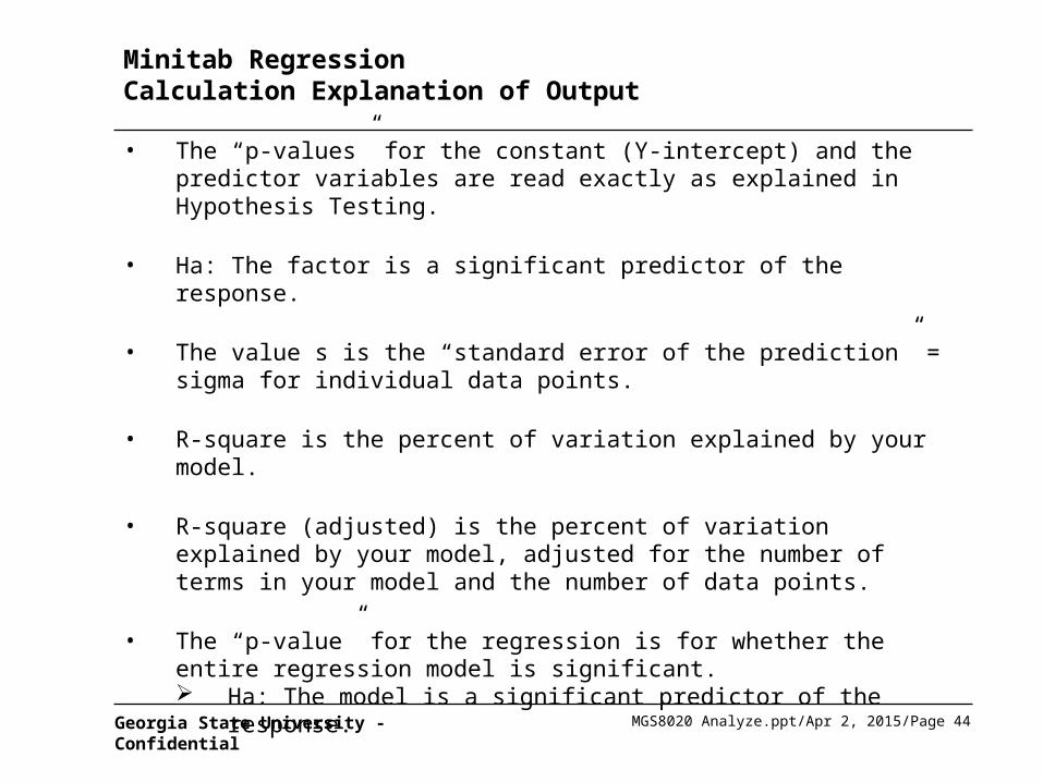
Minitab RegressionCalculation Explanation of Output
• The “p-values” for the constant (Y-intercept) and the predictor variables are read exactly as explained in Hypothesis Testing.
• Ha: The factor is a significant predictor of the response.
• The value s is the “standard error of the prediction” = sigma for individual data points.
• R-square is the percent of variation explained by your model.
• R-square (adjusted) is the percent of variation explained by your model, adjusted for the number of terms in your model and the number of data points.
• The “p-value” for the regression is for whether the entire regression model is significant. Ha: The model is a significant predictor of the response.
MGS8020 Analyze.ppt/Apr 2, 2015/Page 45Georgia State University - Confidential
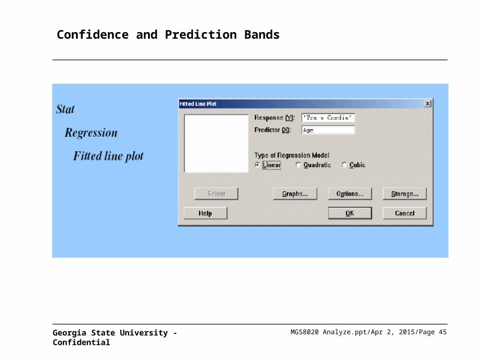
Confidence and Prediction Bands
MGS8020 Analyze.ppt/Apr 2, 2015/Page 46Georgia State University - Confidential
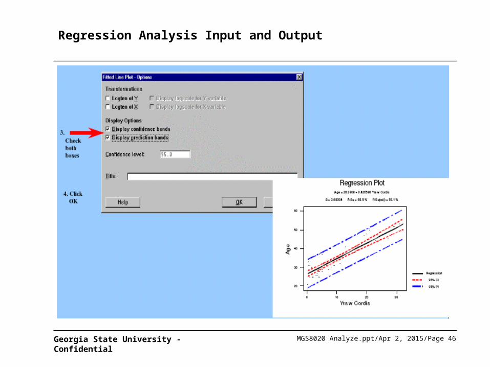
Regression Analysis Input and Output
MGS8020 Analyze.ppt/Apr 2, 2015/Page 47Georgia State University - Confidential
Regression Analysis – Confidence and Prediction Bands
• A confidence band (or interval)
A measure of the certainty of the shape of the fitted regression line
In general, a 95% confidence band implies a 95% chance that the true line lies within the band. [Red lines]
• A prediction band (or interval)
A measure of the certainty of the scatter of individual points about the regression line
In general, 95% of the individual points (of the population on which the regression line is based) will be contained in the band. [Blue lines]
MGS8020 Analyze.ppt/Apr 2, 2015/Page 48Georgia State University - Confidential
Regression Analysis – Summary
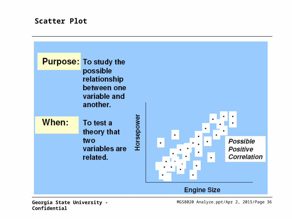
• Scatter Plots: Visual tool to establish a cause and effect relationship between the inputs and the outputs.
• Simple Linear Regression Statistical technique used to investigate the relationship between 2
variables Ha: The factor is a significant predictor of the response R2: percent of variation explained by yourmodel. In general, the closer
R2 is to 1, the better the fit of the model Prediction Intervals: 95% of data within the population falls within this
band Confidence Intervals: There exists a 95% chance that the true line of
the population lies within the band Prediction Interval: Can be used in statistical tolerancing
MGS8020 Analyze.ppt/Apr 2, 2015/Page 49Georgia State University - Confidential
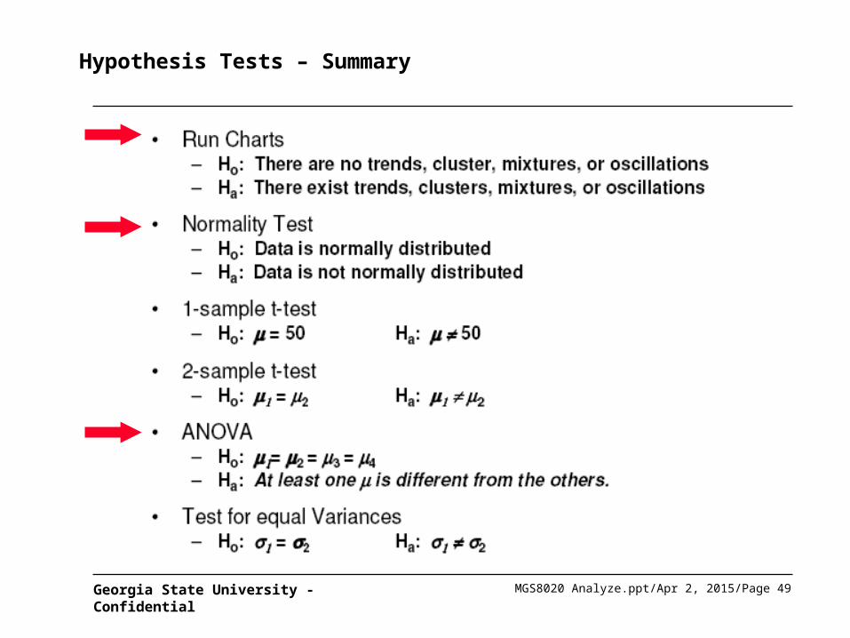
Hypothesis Tests – Summary