AFRL-IF-RS-TR-1999-133 In-House Report May 1999

METHODS OF DISCRETE-TIME PHASE AND FREQUENCY SYNCHRONIZATION

Andrew J. Noga

APPROVED FOR PUBLIC RELEASE; DISTRIBUTION UNLIMITED

19990712 024 AIR FORCE RESEARCH LABORATORY

INFORMATION DIRECTORATE ROME RESEARCH SITE

ROME, NEW YORK

DTCC QUALITY INSPECTED 4

This report has been reviewed by the Air Force Research Laboratory, Information Directorate, Public Affairs Office (IFOIPA) and is releasable to the National Technical Information Service (NTIS). At NTIS it will be releasable to the general public, including foreign nations.

AFRL-IF-RS-TR-1999-133 has been reviewed and is approved for publication.

APPROVED: ^P^J^^/^O

GERALD C. NETHERCOTT Chief, Multi-Sensor Exploitation Branch Info and Intel Exploitation Division Information Directorate

FOR THE DIRECTOR: \Uyn ß^/Ccift t^M, t

( JOHN V. MCNAMARA, Technical Advisor Info and Intel Exploitation Division Information Directorate

If your address has changed or if you wish to be removed from the Air Force Research Laboratory Rome Research Site mailing list, or if the addressee is no longer employed by your organization, please notify AFRL/IFEC, 32 Brooks Road, Rome, NY 13441-4114. This will assist us in maintaining a current mailing list.

Do not return copies of this report unless contractual obligations or notices on a specific document require that it be returned.

REPORT DOCUMENTATION PAGE Form Approved OMB No. 0704-0188

Public reporting burden for this collection of information is estimated to average 1 hour per response, including the time for reviewing instructions, searching existing data sources, gathering and maintaining the data needed, and completing and reviewing the collection of information. Send comments regarding this burden estimate or any other aspect of this collection of information, including suggestions for reducing this burden, to Washington Headquarters Services, Directorate for Information Operations and Reports, 1215 Jefferson Davis Highway, Suite 1204, Arlington, VA 22202-4302, and to the Office of Management and Budget, Paperwork Reduction Project (0704-0188), Washington, DC 20503.

1. AGENCY USE ONLY (Leave blank) 2. REPORT DATE

May 1999 3. REPORT TYPE AND DATES COVERED

In House, April 1996 - April 1999 4. TITLE AND SUBTITLE

METHODS OF DISCRETE-TIME PHASE AND FREQUENCY SYNCHRONIZATION 6. AUTHOR(S)

Andrew J. Noga

5. FUNDING NUMBERS

PE -62702F PR - 4594 TA-15 WU-A2

7. PERFORMING ORGANIZATION NAME(S) AND ADDRESS(ES)

AFRL/IFEC 32 Brooks Road Rome, NY 13441-4114

8. PERFORMING ORGANIZATION REPORT NUMBER

AFRL-IF-RS-TR-1999-133

9. SPONSORING/MONITORING AGENCY NAME(S) AND ADDRESS(ES)

AFRL/IFEC 32 Brooks Road Rome, NY 13441-4114

10. SPONSORING/MONITORING AGENCY REPORT NUMBER

AFRL-IF-RS-TR-1999-133

11. SUPPLEMENTARY NOTES

Air Force Research Laboratory Project Engineer: Andrew Noga/IFEC/315-330-2270.

12a. DISTRIBUTION AVAILABILITY STATEMENT

Approved for public release; distribution unlimited.

12b. DISTRIBUTION CODE

13. ABSTRACT (Maximum 200 words)

Further analysis of the reconstituted numerical FM with feedback (RNFMFB) has been performed, and these results are presented. It is shown that the RNFMFB demodulator is capable of achieving both phase and frequency synchronization in discrete-time applications. In contrast to the digital phase locked loop (DPLL), the RNFMFB is simple to use and can operate at low sampling rates. In addition to providing low SNR threshold enhancement, the RNFMFB demodulator also provides enhancement as the input SNR increases above threshold. This is again, in contrast to currently employed DPLL algorithms which can only provide threshold enhancement. Simulations and analyses are presented which verify this performance enhancement achieved by the RNFMFB demodulator.

14. SUBJECT TERMS

numerical demodulation, frequency feeddback, discrete-time signal processing 15. NUMBER OF PAGES

84 16. PRICE CODE

17. SECURITY CLASSIFICATION OF REPORT

UNCLASSIFIED

18. SECURITY CLASSIFICATION OF THIS PAGE

UNCLASSIFIED

19. SECURITY CLASSIFICATION OF ABSTRACT

20. LIMITATION OF ABSTRACT

UNCLASSIFIED U/L Standard Form 298 (Rev. 2-89) (EG) Prescribed by ANSI Std. 239.18 Designed using Perform Pro, WHS/DIOR, Oct 94

TABLE OF CONTENTS

List of Abbreviations iv

List of Conventions v

1 Introduction 1

1.1 The PLL Paradox 2

1.2 The Phase Lock Fallacy 3

1.2.1 Phase Estimation Using Feedback 3

1.2.2 Alternatives to the DPLL 6

1.3 Note on Notation 7

2 Filtering the Phase of a Complex Exponential Sequence 8

2.1 Practical Considerations 8

2.2 Filtered Phase Estimation Performance 10

2.2.1 Further Comments on Performance 12

2.3 An Example Application: Carrier Synchronization for M-ary Phase Detection 14

2.3.1 FM Discriminator-based Carrier Synchronization 14

2.3.2 FM Discriminator-based Modulation Recovery Results 17

2.3.3 Improvements to M-ary PSK Demodulation 20

3 A Novel Discrete-Time Synchronous Demodulator 23

3.1 Employing Feedback in Angle-demodulation 23

3.1.1 Enhanced Band-pass Filtering 24

3.1.2 Current Limitations and Disadvantages of Feedback Angle-demodulation 28

3.2 Reconstituted Numerical FM with Feedback (RNFMFB) Demodulator 29

3.2.1 Achieving Phase Synchronization in the RNFMFB Demodulator 32

3.3 An Example Application: Carrier Synchronization for M-ary Phase Detection 33

3.3.1 RNFMFB Demodulator-based Carrier Synchronization 33

3.3.2 RNFMFB Demodulator-based Modulation Recovery Results 35

3.3.3 Further Comments on Results 37

4 Conclusions 39

4.1 Summary of Findings 39

4.1.1 FM Discriminator-based Synchronization 40

4.1.2 Synchronization Using the NFMFB Demodulator 41

4.1.3 Synchronization Using the RNFMFB Demodulator 41

4.1.4 Simplification of the NFMFB Demodulator 42

4.1.5 Required Sampling Rates for the DPLL 43

4.1.6 DPLL Complexity 44

4.1.7 RNFMFB Simplicity 44

4.2 Required Further Research 44

4.2.1 Integration Accuracy 45

4.2.2 Quantization Effects 46

4.2.3 The Arctan Process 46

4.2.4 Methods of Lock Indication 47

4.2.5 Filter Design 47

4.2.6 Transient Analysis 48

4.3 Final Comments 49

APPENDIX A - A Quick Look at the Numerical FM with Feedback (NFMFB) 50 Demodulator / Digital Phase-Locked Loop (DPLL)

A.0 The Need for a "Quick Look" at the NFMFB 51

A. 1 NFMFB Demodulation for Carrier Synchronization for M-ary Phase Detection 51

A. 1.1 First-Order NFMFB Demodulator Examples 52

A. 1.2 Second-Order NFMFB Demodulator Example 56

A. 1.3 Proportional Plus Integrator NFMFB Demodulator Example

A.2 Additional Comments

58

60

APPENDIX B - Filter Response Plots

B.O Appendix Description

B.l Section 2.3.2 Filters

B.2 Section 3.3.2 Filters

B.3 Section A. 1.1 Filters

B.4 Section A. 1.2 Filters

B.5 Section A. 1.3 Filters

61

62

63

64

66

68

69

References 71

in

LIST OF ABBREVIATIONS

ADC Analog-to-Digital Converter

AFOSR Air Force Office of Scientific Research

AFRL Air Force Research Laboratory

BPF Band-pass Filter

DPLL Digital Phase Locked Loop

DSP Digital Signal Processing; Digital Signal Processor

DTL Digital Tanlock Loop

ER Entrepreneurial Research

FIR Finite Impulse Response

FM Frequency Modulation; Frequency Modulated

FMFB Frequency Modulation with Feedback (demodulator)

IIR Infinite Impulse Response

LPF Low-pass Filter

NCO Numerically Controlled Oscillator

NFMFB Numerical FM with Feedback (demodulator)

PLL Phase Locked Loop

PSK Phase Shift Keyed

RNFMFB Reconstituted Numerical FM with Feedback (demodulator)

SNR Signal-to-Noise Ratio

VCO Voltage Controlled Oscillator

iv

LIST OF CONVENTIONS

representative examples:

a positive constant amplitude of a modulated complex envelope signal

a(nTs) a phase modulation sequence (radians)

b(nTs) an observation from the random process of a positive amplitude sequence

ß FM modulation deviation ratio

fe tuning frequency error (Hz)

fm essential bandwidth of a message signal (Hz)

7](nTs) an observation from the random process of a phase distortion sequence (radians)

A(nTs) an observation from the random process of a phase modulation sequence (radians)

nTs product of an integer index, n, and the sampling time interval, Ts, seconds

s+ {nTs) a transmitted generalized positive pre-envelope signal

v the estimate of some quantity, v; e.g., A is an estimate of A

w+ (nTs) an observation from the random process of an additive noise generalized positive pre-

envelope signal

x+ (nTs) an observation from the random process of a received generalized positive pre-

envelope signal

1 Introduction

The phase locked loop (PLL) is well known by communication engineers to be a key

component in many receive and signal generating systems. Applications include FM

demodulation, FM stereo reception and indication, carrier and symbol synchronization, co-channel

interference reduction, and coherent signal generation for use in such areas as direction finding.

Although it is a conceptually straightforward servo-mechanism which has logically been adapted

from control systems to solve signal processing problems, implementation and use of the PLL is a

challenging design task that has kept many engineers gainfully employed. As a result of its

widespread use and subtle characteristics, the PLL has been the subject of numerous journal and

conference papers, is treated in most communications textbooks, and has been the sole subject of

entire textbooks (see e.g., [1-2]).

In recent years, attention has turned from analog (continuous-time, continuous-amplitude)

systems, to digital l (discrete-time, discrete-amplitude) systems, with the advancements in the

state-of-the-art of Analog-to-Digital Converters (ADCs), and programmable digital signal

processors (DSPs). With these enabling technologies, numerical (digital) implementations of

traditionally analog processes including the PLL, have become economically and technically

attractive alternatives. Economically, products can be designed to have generic application, with

changes required only in the program code when applications or specifications change. This can

shorten time-to-market, reduce production overhead, and allow re-use. Technically, there are

processes that are easily accomplished numerically, but extremely difficult to accomplish in analog

form. An example of this is the symmetric finite impulse response (FIR) filter [3] which achieves

a linear phase response over frequency; an analog equivalent is difficult to achieve. In addition,

numerical systems are stable with age and variations in temperature, are exactly repeatable, and

do not suffer from the effects of impedance mismatch when cascaded. Thus, research which

focuses in the area of numerical implementations of communication signal processing systems is

of great technical and economical importance.

1 Here, the term "digital" should not be confused with the notion of symbol transmission in digital communications. To avoid this confusion, this report uses the term "numerical" to describe discrete-time, discrete-amplitude processing.

This report focuses on a novel form of signal processing servo-mechanism, the

reconstituted numerical FM with feedback (RNFMFB) demodulator. As will be shown, the

RNFMFB accomplishes the goal of the PLL, frequency and phase synchronization, with the

associated advantages of numerical processing. Originally introduced in [4] as a method of FM

demodulation enhancement, this report presents the results of recent research regarding the

RNFMFB demodulator, which has been supported by both the Air Force Office of Scientific

Research (AFOSR) Entrepreneurial Research (ER) program, and by the Information Directorate

of the Air Force Research Laboratory (AFRL).

The report is organized as follows: the remainder of this chapter provides further

motivation for the research, and comments on mathematical notations used within the report;

Chapter 2 introduces the concept of filtering phase in numerical systems, and provides results

from an M-ary Phase Shift Keyed (PSK) carrier synchronization simulation; Chapter 3 provides

further analysis of the RNFMFB demodulator as applied to phase and frequency synchronization,

along with results from an M-ary PSK carrier synchronization simulation; and finally, Chapter 4

provides conclusions and future work. Appendices are included which help to support the

material in the main body of the report by providing further simulations and filter response

information in a convenient location.

1.1 The PLL Paradox

At first glance, many engineers would question the need to conduct further research in

PLL design and analysis, or on FM demodulation methods, given the wealth of literature that

already exists on these subjects. Even so, recent literature does exist on these subjects [5-7], and

tends to address numerical implementations, demonstrating interest in taking advantage of

advancements in ADC and DSP hardware [8]. However, it is interesting to note that one

important motivation to conduct research on numerical implementations of the PLL, seems to

have been overlooked.

The Shannon/Nyquist sampling theorem [3], simply stated, indicates that a real analog

signal of bandwidth B, can be completely represented by samples of the signal taken at uniform

intervals of time step, Ts, where Fs = 1 / Ts > 2B. (This includes not only low-pass signals, but

also band-pass signals that can be down-converted in frequency to a center frequency of 5/2 Hz.

Signals that can be represented in analytic form, require a sample rate as low as Fs> B.) The

benefits of using the minimum required sample rate include the obvious reduction in processing

and storage of signals, and less obvious facts such as the reduction in filter orders required to

achieve a given time support and ensuing frequency response. The PLL paradox is: In light of the

Shannon/Nyquist sampling theorem, why is it the case that numerical (digital) phase locked loop

(DPLL) implementations often require sampling rates that are significantly greater than the

minimum ? (See e.g., [8].) Either the sampling theorem is incomplete as stated above, or this is

an undesirable characteristic of known DPLL algorithms, that has not been properly addressed.

The research presented in this report addresses this issue, and a solution is presented.

1.2 The Phase Lock Fallacy

It is a commonly held misconception that the only method of achieving phase lock that is

available to communications engineers, is the phase locked loop (or variants thereof). In fact, as

will be shown, there are alternatives. Some thoughts are provided here, regarding this confusion.

1.2.1 Phase Estimation Using Feedback

It's not always clear what individual or group of individuals should be credited with a

given idea, but one of the earlier contributors to advancing the notion that feedback can be

employed to enhance FM demodulation, is the author Chaffee [9]. This novel application of

existing control system design, resulted in the device known as the FM with feedback (FMFB)

demodulator, the description of which is given here and in Chapter 3. Subsequent to this paper,

many authors presented comparisons of the performance of the PLL and the FMFB, with differing

2 Versions of the sampling theorem exist that treat the cases of both uniformly and non-uniformly spaced samples; this report will address the case of sampling at uniform time steps.

conclusions. Develet [10] reconciled some of these differences, indicating that the FMFB and

PLL can be considered to be equivalent servo-mechanisms. Ultimately, the PLL became far more

popular, do to the simplicity of the device relative to the FMFB demodulator.

Without this background, when considering the application of the PLL to achieve phase

synchronization, it is not intuitive that such a device would enhance this process. Most

measurement processes are open-loop systems; no feedback signal is required to control aspects

of the measurement process. Feedback tends to be employed where the goal is to set or control

some form of operating point. For example, a thermometer can be used to measure the

temperature of a room, but if we wish to maintain a particular room temperature, the heat

source/sink requires some form of measured temperature feedback signal to control the

production or removal of heat. When the temperature rises above the desired set point, heat is

either removed or allowed to dissipate; when the temperature is below the desired set point, heat

is generated until the desired temperature is reached. In contrast, the PLL attempts to measure

phase by controlling a locally generated phase signal, compares this generated phase to the

incoming signal phase, and uses this error signal as feedback to modify the generated phase.

Using the analogy of temperature measurement, this would be equivalent to controlling the

temperature of a room, A, adjacent to the room, B, of interest. The difference in temperature

between the two rooms would be measured, and the temperature of room A would be controlled

using this difference signal as feedback. Once room A achieved the temperature of room B, this

temperature to which room A has been set, would be reported as the temperature of room B. As

with temperature measurement, use of the PLL for phase measurement appears, at first, to be an

unnecessarily complicated approach. The fact that researchers considered the use of a PLL may

have stemmed in part from their knowledge of the more intuitive FMFB demodulation approach.

A base-band representation of the FMFB demodulator is shown in Figure 1-1.

Referencing the work of Chaffee and others since, the intent of the FMFB demodulator is to

reduce the bandwidth of the input signal such that a band-pass filter (BPF) of narrower bandwidth

can be used to reject more noise than would otherwise be possible. This additional noise rejection

results in an enhanced FM estimate, when the system can track the input frequency. In effect, the

FMFB demodulator becomes a band-pass filter, with dynamically changing center frequency.

This center frequency is controlled by measuring the difference between the input phase and a

locally generated phase, and providing this difference as feedback to the local generator. As seen

in the figure, the Phase Detector measures the difference between the phase of the input signal

and the Voltage Controlled Oscillator (VCO) output phase. The Phase Detector output is

differentiated with respect to time, filtered and amplified in the Loop Filter, resulting in a

frequency feedback error signal. This error signal is used to control phase generation in the VCO,

resulting in the frequency tracking ability of the device.

Input Signal

Complex Multiplier v

Phase Detector

> \

> BPF >

^rctan[]

Output cos[] -sin[] Phase ♦ ♦ \dt << <— LPF < d

dt H Voltage Control] led Oscillai tor

_/ complex signal

—*~ real signal

Figure 1-1. A Base-band representation of the FMFB demodulator.

The FMFB demodulator works well for FM signals with specific characteristics, but does

not readily provide phase estimation. This is due to the fact that the FMFB device operates on

the derivative of the phase, which eliminates any constant phase term. Re-establishing this

constant in a subsequent integration process, is difficult to achieve in analog systems. In lieu of

this, when the phase constant is of interest, the differentiation process can be eliminated in the

FMFB device, resulting in a form of PLL. The desire for even further simplification leads to the

elimination of the band-pass filter, BPF. Unfortunately, this also eliminates the intuition which

motivates the consideration of employing feedback to measure phase.

As it turns out, the PLL is found in practice to enhance both the FM demodulation and

phase estimation processes. The device would certainly not be the subject of widespread

research, if this were not the case. It is proposed in this report, based on the research results

presented and referenced, in the absence of the BPF this enhancement is due to the fact that the

PLL reduces the modulation index of the input signal, and eliminates tuning offsets. As shown in

[4] for discrete-time systems, the probability of occurrence of phase cycle-skips increases when

either modulation, tuning offsets, or both, are present. As input signal-to-noise ratio (SNR) is

decreased, a threshold is reached beyond which the performance of angle demodulation systems

degrade rapidly. This threshold is characterized by the onset of phase cycle-skips, and is therefore

reduced by the PLL when the modulation index and tuning offset are reduced. Threshold

enhancements of 3 to 6 dB have been reported in the literature.

A final point should be made with regard to the base-band FMFB representation given in

Figure 1-1. Referring to the figure, the Phase Detector has been idealized by the use of the

y4rctan[-] process. Note that this is not easily accomplished in analog form [11], but is readily

employed in numerical systems [12].

1.2.2 Alternatives to the DPLL

Unfortunately the widespread use of the analog PLL for the phase estimation process, has

lead to the misunderstanding that only a numerical (digital) PLL implementation, the DPLL, can

provide effective discrete-time phase and frequency estimation. As indicated above, a numerical

implementation of the FMFB demodulator is at least one example where, within a phase constant,

we can expect to achieve effective phase and frequency estimation. (The ^4rc tan[] calculation

itself can be considered to be a viable method of phase estimation [13], and although widely used

in various applications, it is seldom presented as a phase synchronization device, although this

description is a valid one.) A second example that can be given is what could be described as a

discrete-time phase-synchronous FM discriminator, which is presented in Chapter 2. In fact, as

with the FIR filter, this FM discriminator-based phase estimator is another example where a

numerical implementation can achieve what would normally be extremely difficult in the analog

realm. Namely, through judicial choice of initial conditions, the phase constant eliminated by

numerical approximation to differentiation, can be exactly and easily recovered. Moreover,

because the phase-synchronous FM discriminator can be used within the numerical FMFB

demodulator (NFMFB), acceptable phase synchronization can also be achieved by the NFMFB

device. These results will be presented in Chapter 3 and Appendix A. Finally, a third method of

discrete-time phase and frequency synchronization is also presented in Chapter 3. Here, the

concept of signal reconstitution within the NFMFB is introduced, resulting in a novel form of the

device which attains phase and frequency synchronization at the minimum sample rate required by

the Shannon/Nyquist sampling theorem. At the same time, the input SNR threshold is reduced by

temporarily reducing the modulation index and tuning offset. Also, band-pass filtering is

accomplished which rejects out-of-band noise and further reduces the threshold. Design

considerations are greatly simplified, when using the newly proposed device.

1.3 Note on Notation

As with any technical endeavor, careful choice of mathematical notation can improve the

readability of written descriptions of conducted research, and the same is true here. In light of

this, and since the presented analytical results are given along with experimental observations, the

often used approach of employing random variable notation is avoided. Instead, the variables

presented are considered to be sample functions (sequences) from random processes, i.e., a

specific observation signal sequence resulting from a simulation run.

In the next chapter, a detailed analysis will be given regarding FM discriminator-based

discrete-time phase and frequency synchronization. Results will be given for the application of M-

ary PSK carrier recovery and symbol detection.

2 Filtering the Phase of a Complex Exponential Sequence

2.1 Practical Considerations

Given a complex exponential sequence of the form

X+(nTs) = b(nTs)exp{j-A(nTs)}, b(nTs)>0, (2-1)

we are interested in the sequence

y+(nTs) = exP[j-A(nTs)*h(r1Ts)}. (2-2)

Here, b(nTs) and A(nTs) are respectively the (real-valued) envelope and phase sequences of

x+(nTs), and h(nTs) is the impulse response of a realizable filter. Note that from Eq. (2-1),

b(nTs) is readily recovered from x+(nTs), at any instant in time, nTs. However, this is not the

case for proper recovery of A(nTs). The method to be employed herein for phase sequence

recovery requires estimation of the rate-of-change-of-phase,

for recovery of the phase sequence [4]. This implies the use of more than a single sample for

recovery of each sample of A.

By forming the first-backward-difference sequence

d(nTs) = g[^ (nTs) - ^ ([« - \]TS)], (2-3)

we can then find d{nTs)* h(nTs), and subsequently accumulate this result to remove the effect of

the difference calculation. In Eq. (2-3) the modulo-27i process , g[-], is

g[a] = {a + 7v) mod 2K - 7z, (2-4)

and the instantaneous phase sequence, Aln (nTs), is

A2AnTs) = g[A(nTs)], (2-5)

as recovered by a four-quadrant arctangent calculation. Thus an estimate, A(nTs), of the true

phase sequence, A(nTs), can be formed as

3 Here, we are using the definition {x} mod v = X - V • kv, where kv is an integer such that {x} mod v lies in the interval between 0 and v , inclusive of 0.

Ä(nTs) = ^d(kTs) + Ä2A0) (2-6) 4=1

The goal, however, is to form an estimate of the filtered sequence, A(nTs)* h(nTs). This

is accomplished by first forming

y(nTs) = d(nTs)*h(nTs), (2-7)

which represents the filtered instantaneous frequency estimate. Setting d(0) = X^n (0), from the

principal of superposition along with Eqs. (2-6) and (2-7) we have that4

*=0 k=0

= h(nTs)*'Zd(kTs) k=0

= A(nTs)*h(nTs). (2-8)

Eq. (2-8) demonstrates that the accumulation of the filtered instantaneous frequency estimate is

equivalent to applying the same filter to the recovered phase estimate, X(nTs).

Note that in many scenarios, it is only necessary to retain this filtered phase sequence in a

modulo-27t fashion. This is the case for the sequence y+ (nTs) identified in Eq. (2-2). In practice

we are limited to using the estimate

y+{nTs) = Qxp{j-A(nTs)*h(nTs)} . (2-9)

In this case the sum given in Eq. (2-8) can be retained modulo-27r. In lieu of Eq. (2-8) when, for

example, the further goal is to estimate y+ (nTs), we form

g[knTs)*h(nTs)] = gt,g[y(kTs)\

f,g[d(kTs)*h(kTs)] = g (2-10)

4 Setting d(0) = A^ (0) equates to the arbitrary but convenient initial condition XlK (-7^ ) = 0. The

same initial condition is used in the integration process of Eq. (2-8).

This modulo-271 integration process is depicted in Fig. 2-1. Note that the method of Eq. (2-10)

bounds the result in the range [-it,%) for implementation purposes. Here, we have taken

advantage of the complex exponential property

expfy'-x} = exp{./-g[x]}. (2-11)

p \ z\i(nT)*h(nT) rs)

*KnTs) +>ft p- *n

+ k

T. Delay

Figure 2-1. Block diagram representation of Eq. (2-10).

2.2 Filtered Phase Estimation Performance

Of interest is how well the sequence of Eq. (2-9) estimates the sequence of Eq. (2-2). We

proceed by considering the intended effect of filtering the phase as in Eq. (2-2). Implicit in this

requirement is that A(nTs) is composed of many constituents, only one (or the sum of a set) of

which is of interest. The filtering process is meant to take advantage of spectral characteristics of

the desired component relative to the undesired components of A(nTs). Decomposing A(nTs)

we have

MnT,) = «nT,) + e(nTa) (2-12)

where 0(nTs) is some desired component of A(nTs), and e(nTs) is the undesired component.

10

Errors arise in using Eq. (2-3) when instantaneous frequency aliasing [4] of <j>(nTs) occurs

as a result of the additive error component, e(nTs). From Eqs. (2-3) and (2-12) along with

properties of modulo arithmetic we have that

d(nTs) = g[<t,(nTs) - <f>{[n - l]Ts) + g[e'(nTs)]} (2-13)

where

e'(nTs) = e(nTs)-e([n-\]Ts). (2-14)

The error in approximating y+(nTs) by using Eqs. (2-9), (2-10) and (2-11) can be assessed

(normally in a probabilistic sense) when we have enough knowledge regarding e and <f> (such as

their joint amplitude distribution and correlation from sample to sample). Note that in forming

Eq. (2-3), it has been implied that any known bias in the phase angle difference has already been

removed such that what remains is an unknown bias, 2jufeTs. The phase error itself can be

decomposed into the sum of a bias-induced term, a local oscillator phase offset, 0, and a

distortion constituent, rj(nTs), as

e(nTs) = 2nfenTs -0+?j(nTs). (2-15)

From Eqs. (2-14) and (2-15) we have that

e'(nTs) = 2nfeTs+Jj'(nTs) (2-16)

where

n'{nTs) = rj(nTs)-ri([n-l]Ts). (2-17)

Applying properties of modulo-27i arithmetic in Eq. (2-13), we can define fe and rj(nTs) such

that the properties

-7i<2nfeTs<+7v (2-18)

and

-n< rj(nTs) < +n (2-19)

both hold. By design, the desired phase component should have the property

-n<<t>{nTs)-<l>{[n-\]Ts)<+7T. (2-20)

11

Eq. (2-20) identifies a property of the desired phase component, ^, and represents an additional

requirement on the sample interval, Ts. Of course, the sample interval must also be chosen such

that tolerable destructive aliasing occurs when sampling the original continuous-time signal, <j>(t).

2.2.1 Further Comments on Performance

It can be difficult to assess the performance of phase estimators, and this holds true for the

FM discriminator-based estimator as well. The intent of introducing Eqs. (2-12) through (2-20) is

to gain some insight into the various mechanisms by which error is introduced by this particular

estimator. In the absence of distortion, TJ , we can identify the phase modulation sequence

a(nTs) = 2nfenTs+<f>(nTs)-0. (2-21)

This phase modulation is a result of both the desired (message bearing) component, <f>, and

receiver tuning errors. Note that even in the ideal case where no distortion is present, we do not

have access to a. This fact is made more evident by representing a as

a{nTs) = ^a(nTs)] + lit • ra (nTs)

= a2„(nTs) + 2n-ra(nTs), (2-22)

where ra {nTs) is an integer valued sequence such that the equality in Eq. (2-22) holds. From the

complex exponential property identified in Eq. (2-11), it is apparent that we are unable to recover

a completely. In employing the backward difference FM discriminator, we are in effect

attempting to estimate the sequence ra. In this distortion-free case, when Eq. (2-18) and (2-20)

hold and -7t<2rtfeTs + <p{nTs)-<j>(\n-X\Ts)<+K, we are able to estimate ra to within some

constant but unknown multiple of 2n.

In practical situations where distortion is present, we have from Eqs.(2-12), (2-15) and (2-

21) that

Ä{nTs) = a{nTs) + n{nTs). (2-23)

In the process of estimating A using the FM discriminator, we obtain [4]

A(nTs) = a2jt (nTs ) + 2x-ra (nTs) + rj(nTs)

12

= a(nTs ) + 2ir-re (nTs) + rfciT,), (2-24)

where re is

re(nTs) = ra(nTs)-ra(nTs). (2-25)

The error sequence, re (nTs), is referred to as the sheet sequence error, since it represents the

error in determining the actual sheet sequence, ra(nTs). The phase cycle-slip, 2n-r'e{nTs},

resulting from backward difference FM discrimination, is related to re as

27frXnTs) = 27r-{re{nTs)-re([n-\]Ts)}. (2-26)

We are now able to better assess the performance of the estimator identified in Eq. (2-9).

The purpose of the low-pass filter, h, is to reject the distortion, rj, but not at the expense of

rejecting the phase modulation, a. These components are identified in Eq. (2-24). Also present,

however, is the term 2n ■ re (nTs). The linear low-pass filtering process can help to eliminate

error due to this term, but it is not normally taken into consideration when designing h. The

reason for this is that spectrally, this term contributes uniform energy across the entire Nyquist

band. Overall, our FM discriminator-based phase modulation estimate, ä, is identified as

«([» ~nL]Ts) = i{nTs )* h(nTs), (2-27)

which from Eq. (2-24) becomes

ä([n-nL]TJ = a(nTs)*h(nTJ + 27r-re(nTJ*h(nTJ + rj(nTs)*Kr1Ts). (2-28)

Here, nLTs is a value representing the best approximation to the time delay introduced by the

filter, h. Eq. (2-28) demonstrates that the FM-discriminator-based phase estimator is a valid

method of discrete-time phase synchronization. A particular advantage of this technique is that

the acquistion time is commensurate with the essential length of the filter impulse response. (In

the distortion-free case, there is no need for h, and the acquisition is instantaneous.) Note that

Eq. (2-28) also allows us to predict performance of the FM discriminator-based phase estimator

when we have knowledge of a and TJ , such that the ensuing phase cycle-slip error arising in Eq.

(2-6) can be assessed.

13

2.3 An Example Application: Carrier Synchronization for M-ary Phase Detection

To promote the understanding of the FM-discriminator-based phase estimator, it is

instructive to present an application of the technique. The performance of the FM-discriminator-

based phase estimator can also serve as a baseline against which other methods can be compared.

The example given is that of carrier synchronization for subsequent recovery of an arbitrary

symbol sequence, m{nTs), which has been imposed on the phase of the signal of interest.

2.3.1 FM Discriminator-based Carrier Synchronization

The received signal is modeled as an M-ary phase modulated signal in additive white

Gaussian noise, and is represented in complex envelope form. This received signal, x+, is as in

Eq. (2-1). For M-ary phase-shift-keyed (PSK) modulation, the message bearing signal, $, is

</>(nTs) = ^-m{nTs),

f-M + 1 -M + l M-l] wej—-—,—-— + 1,...,—^— J- forModd,

f- M - M M\ m e<K- + 1>-y- + 2>->y] forMeven, (2-29)

where M is an integer, M>2. The common method of carrier recovery for the M-ary phase

signal, is to raise the received signal to the power M, which effectively eliminates the message

bearing signal, ^. (i.e., g[M-^(w7^)j = 0.) The phase of the resulting complex signal contains a

term which is M times the desired carrier phase. This signal is then typically processed by a

Phase-Lock Loop (PLL) with divide by M capability, to track the carrier phase [13].

Equivalently, one can convert the received signal from rectangular to polar coordinate

representation, multiply the phase by M, and subsequently apply some form of phase tracking and

scaling by MM, to generate the carrier phase estimate. In this example, the FM discrimination and

integration processes provide the phase tracking mechanism.

i.e., spectrally uniform across the complex Nyquist band, [—n, 7t) sample-rate-normalized radians.

14

Referring to Figure 2-2, one method of using FM discrimination and integration for M-ary

PSK carrier recovery is shown. Note that the intent in this report is not to present the "best"

method of processing the received PSK signal. However, the method shown is certainly worthy

of performance evaluation, since it represents a very practical solution.

*+m a) > Arc tan

\A»TS) MA2AnTs)

M cosine[ ] sine[ ]

z+(«r,) = exp{y.Ml(«ri)}

z>

MnrjexpfMOiJ,)} z+(nTs) . j\

b) Z>*^(»T;)Z> Arc tan

Delay

\

c) jj-g[U«T.)-W-W,Jl

**h{nTs) +

+ *H

T. Delay

ac([n-n„]T,)

Figure 2-2. Processing steps for carrier recovery from an M-ary phase signal; a) step 1: message removal, b) step 2: Backward-difference FM discrimination, c) step 3: low-pass filtering and integration.

As shown, the method can be described as three separate processing steps including message

removal, FM discrimination and integration. Figure 2-2 a) shows the first step of message

removal. The input is the (complex) received signal, x+ {nTs), as previously described. It is

represented in rectangular form by the pair of signals, / and q, where / is used to refer to the "in-

phase" component of a complex signal, and q is used to refer to the "quadrature" component.

15

(For notational convenience, the dependency on time, nTs, is left as implicit.) The four-quadrant

arctangent calculation (Arctan) produces the phase sequence A2„(nTs) = g[A(nTs)\, which is

multiplied by M, and then used to modulate the phase of a unit amplitude complex exponential.

Properties of modulo arithmetic allow us to represent this output as z+ (nTs) = expy- MA(nTs)\.

This signal, z+ (nTs), contains information regarding the carrier phase of interest, but the message

sequence has intentionally been eliminated. It can easily be shown that z+ (nTs) is a tone at M

times the tuning offset frequency with M times the phase of the non-message portion of the phase

of the received signal. We now need to extract this phase and scale by the factor MM, to arrive at

a carrier phase estimate.

This is accomplished in step 2 shown in Figure 2-2 b), using the backward-difference FM

discriminator. Here, the signal z+(nTs) is first band-pass filtered (using a pair of identical real

low-pass filters, each operating on the / and q signals independently) using the complex filter hB.

The output of this filter has some envelope, bx, and phase, Ax, as shown. The purpose of the

filtering is to remove out-of-band noise. Note that the design of this filter is dependent upon how

well we know the tuning error associated with x+ (nTs). The cut-off frequency of the low-pass

filter pair can be set to M-fe, but no lower. Thus the effectiveness of this filter in removing

noise is limited by the tuning accuracy. Subsequent backward difference FM discrimination and

scaling by the factor XIMresults in the real signal (1 / M) • g[/L, («7^)-Al([n- 1]TS)].

This signal can be low-pass filtered and integrated to generate the carrier phase estimate,

as shown in Figure 2-2 c). The low-pass filter, h, operates as before and further removes noise

and distortion from our estimate, Al. In this specific case, this filter need only pass the d.c. term,

27rfeTs, arising from the tuning offset. Practically speaking, the filters hB and h are chosen such

that the total sample (group) delay introduced by these filters, n0=nB+nL, is kept small. This

group delay is extremely relevant, since the goal here is phase synchronization. Ability to

synchronize in phase to the received signal is dependent on time delays introduced in the

synchronization process. Therefore, referring to the actual carrier phase of the received signal as

16

ac(nTs), we acknowledge any time delays in the FM discriminator method of carrier

synchronization by referring to the estimated phase as ac([n - n0]Ts). This allows for proper use

of this synchronized phase output.

Identifying the actual carrier phase (relative to the receiver) as ac(nTs) = 2nfenTs -0, the

received signal is x+ (nTs) = b(nTs) expjy • [ac (nTs) + </>{nTs) + t](nTs))}. To extract the message

bearing signal, <f>, the received signal is delayed by n0 samples and multiplied by

expi-j-dc([n-n0]Ts)\. M decision boundaries are applied to the phase of the resulting

complex exponential to determine which of M symbols has been transmitted.

2.3.2 FM Discriminator-based Modulation Recovery Results

The simulation results to be presented were obtained by adding sample sequences from a

white Gaussian noise generator to a unit-envelope M-ary phase modulated (PSK) signal. Both

the noise and the modulated signal were (complex-valued) sequences of length 65536 samples.

Simulation runs consisted of varying the input signal-to-noise ratio (SNR) per bit and counting the

corresponding detection errors. Values of SNR per bit ranged from 0 to 12 dB, at 1 dB

increments for each simulation run. Figure 2-3 shows the average of results from 10 simulation

runs for each of three M-ary PSK detection methods. (With 10 simulation runs and 65536

samples per SNR value, we are able to keep the experimental variations low enough to make

meaningful observations down to symbol error rates of about 10"4 [14].) The first of these

methods is referred to as the ideal method, since in this method the known carrier was used to

provide perfect phase synchronization prior to deciding between the M possible phase states. This

method is of course not possible in practice, but it does provide a valuable performance reference.

The second method used was that of the backward-difference FM discriminator with low-pass

filter, as previously described and shown in Figure 2-2. The third method presented is the same

FM discriminator without low-pass filtering, i.e. with h(nTs) = 5{nTs).

In all simulation results to be presented, perfect symbol synchronization is assumed and

the sample interval, Ts, is set equal to the symbol interval, resulting in exactly one sample per

17

symbol. Symbols were randomly generated such that for any particular sample, each symbol was

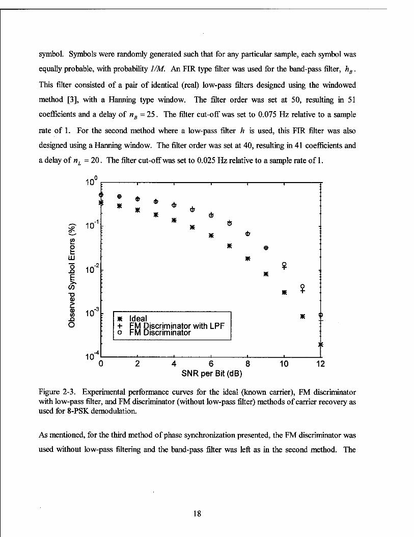
equally probable, with probability 1/M. An FIR type filter was used for the band-pass filter, hB.

This filter consisted of a pair of identical (real) low-pass filters designed using the windowed

method [3], with a Hanning type window. The filter order was set at 50, resulting in 51

coefficients and a delay of nB=25. The filter cut-off was set to 0.075 Hz relative to a sample

rate of 1. For the second method where a low-pass filter h is used, this FIR filter was also

designed using a Hanning window. The filter order was set at 40, resulting in 41 coefficients and

a delay of nL = 20. The filter cut-off was set to 0.025 Hz relative to a sample rate of 1.

10

10"1t

2 LU

O Si E

c/) X3 d) £ <D </) Si O

102k

io-%

10

* *

*

*

*

*

*

K

K

* Ideal +■ FM Discriminator with LPF o FM Discriminator

o

x

4 6 8 SNR per Bit (dB)

10 12

Figure 2-3. Experimental performance curves for the ideal (known carrier), FM discriminator with low-pass filter, and FM discriminator (without low-pass filter) methods of carrier recovery as used for 8-PSK demodulation.

As mentioned, for the third method of phase synchronization presented, the FM discriminator was

used without low-pass filtering and the band-pass filter was left as in the second method. The

18

specific case of M=8 phase states was simulated. The tuning error was set at

/e=.l/(2M) = 0.00625 Hz.

As seen in the figure, for 8-PSK modulation the FM discriminator with low-pass filter

starts to outperform the FM discriminator alone, at or about 9 dB SNR per bit. Below this value,

low-pass filtering does not appear to be justified. As we move above this value, the benefit of

having the low-pass filter becomes more apparent and can be expected to continue for cases of

increasing SNR per bit. Further simulations/analysis are required for input SNR per bit values

beyond 12 dB, to substantiate these expectations. However, we have gained some insight into

performance through Eq. (2-28). It is commonly known that as the input SNR decreases, the rate

of phase cycle-slip occurrences increases. In fact there is a threshold that is eventually reached

beyond which the cycle-slips occur quite frequently. Prior to this threshold, phase cycle-slips

rarely occur. Thus the second term in Eq. (2-28) is expected to adversely affect phase estimator

performance, only when operating at or below this threshold. When cycle-slips occur, the second

term gives rise to instantaneous 2n phase steps which are filtered by h. This leads to an error

signal which starts at the cycle-slip occurrence, and is a function of the filter impulse response.

When multiple phase steps occur, these error sequences are superimposed. Therefore we would

expect the same type of threshold effect when using this device for M-ary PSK carrier

synchronization.

For the general M-ary case, we would expect phase cycle-slips to occur at earlier values of

input SNR as M increases. This is due to the fact that for this application, we modify Eqs. (2-18)

and (2-19) such that fe and rj have the properties - n < 2nMfe Ts < +x and

-n < M-Tj(nTs) < +n. Thus for a particular instant in time and given value of fe, increasing M

increases the probability of occurrence of a phase cycle-slip, by causing an effective tuning error

of M-fe. The cycle-slip rate is further increased, since the required property

-n< M-rj(nTs) <+/r implies a redefinition of TJ. The distribution from which M-rj(nTs) is

sampled more rapidly approaches that of a uniform distribution as SNR is decreased, relative to

the original distribution from which Jj(nTs) is sampled. This implies that the product

M-rj'inTs) will result in values closer to the +l-n boundary a higher percentage of the time

19

than will tj'(nTs). This leads to In IM phase slips in the carrier phase estimation process,

increasing the likelihood that a symbol detection error will occur. Thus the results presented in

Figure 2-3 are consistent with results inferred by Eq. (2-28).

It should be pointed out that in arriving at the results shown in Figure 2-3, symbol errors

were counted differently for the ideal method. Since in the ideal method the carrier phase is

exactly known, a symbol error occurs only when the received symbol is not the same as the

transmitted symbol. This is in contrast to the counting technique use for the FM discriminator-

based methods. For these methods, a change in the difference between the transmitted symbol

sequence and the received symbol sequence from sample n to sample n+1, represents a symbol

error. Thus it is assumed that the transmitted data has been differentially encoded, such that

single phase detection errors often result in two consecutive symbol errors. At best, when using

the FM discriminator-based phase estimator to acquire the carrier of the PSK signal, detection

errors will be twice that of the ideal method unless steps are taken to remove phase ambiguities.

For example, in a cooperative scenario, the receiver may have knowledge of the intended

transmitted phase at periodic time intervals. Provided these intervals are short enough for the

given channel characteristics, phase ambiguity can be removed and phase need not be differentially

encoded. In this case, performance can approach that of the ideal method as SNR per bit

increases. Other improvements to the example application of the FM discriminator-based phase

estimator are also possible.

2.3.3 Improvements to M-ary PSK Demodulation

Improvements on the previously presented method can certainly be made, while

maintaining the same total sample delay, n0. It should be noted that n0Ts represents a measure

of "time-to-lock" contributed by the FM discriminator-based phase estimator. (Alternatively, one

can interpret n0 Ts as a measure of filter settling time.) In the example given, a contribution to

time-to-lock of n0 =nB+nL =45 samples (at one sample per symbol, and 7^ = 1) is achieved.

This is a particularly impressive result! This is in contrast to large time-to-lock values often

20

required when using well-known digital phase-lock loop (DPLL) devices 6 (see e.g., [8]). One

area of improvement addresses the adverse effects of the presence of a tuning error, fe. Recall

that the cut-off of the band-pass filter, hB, can be no less than M times the tuning error.

Therefore, if we can estimate Mfe in a small number of samples prior to phase estimation, tuning

refinement can be made. This allows for a smaller cut-off specification such that hB can more

effectively reject noise. There is an additional benefit in that for a given distortion, M-rj(nTs),

decreasing the tuning offset will decrease the probability of a phase cycle-slip occurrence. To

achieve the same time-to-lock, the order of the band-pass filter can be decreased commensurate

with the additional delay due to the tuning error estimation process.

A second area of improvement involves a decrease in the sampling interval, Ts. This may

be possible by either utilizing the capabilities of the receive system, by interpolation, or some

combination of these. The benefit in decreasing the sampling interval is gained in at least two

areas. The first is the beneficial affect on the consequences of a tuning error. For a given tuning

error, the product 27rfeMTs decreases, which decreases the probability of a phase cycle-slip. The

second benefit is with regard to the fact that the process of raising the received signal to the

power M can lead to aliasing of undesired noise components into the pass-band of the filter, hB.

Thus we expect less noise energy to fold into this pass-band, resulting in enhanced performance.

Unfortunately, a decreased sampling interval implies the need for a commensurate increase in the

order of the band-pass filter, to achieve the same performance. (The low-pass filter is not of

concern, since decimation can be performed with low-pass filtering.) Although the total group

delay (in samples) would increase, actual time-to-lock (in seconds) would remain unchanged,

since the sampling rate must be taken into account. It should be noted that improvements

achieved as a result of decreasing the sampling interval, are with reference to a different received

signal model. The appropriate model is one where some over-sampling already exists, as would

be the case if the sequence resulted from the actual digitization of a properly conditioned M-ary

signal.

6 Kim, Un, and Lee [15], and Cho and Un [16] have continued to make progress with respect to the overall performance and application of the digital tanlock loop (DTL), a form of DPLL.

21

Performance improvement can also be gained by careful selection of the restored

envelope. Referring to Figure 2-2 a), the implementation shown results in the signal z+, having a

constant (unit) envelope. Viterbi and Viterbi [17] have shown that carrier recovery performance

is a function of SNR per bit and of the restored envelope. Their work investigates the use of

various powers of the original envelope, -yji2 + q2 , including the unit envelope, \^ji2 +q2J . It

is interesting to note, however, that the authors have restricted themselves to a moving average

filter with equal tap weights as the band-pass filter, hB. The choice of which envelope to use can

be made independently of the designs of the filters h and hB, such that the total group delay need

not change. It should also be noted that the work presented in [17] assumes that an exterior

process has removed the tuning error. This is in contrast to the FM discriminator-based phase

estimator, which is tolerant to mis-tuning.

In the next chapter, another method of discrete-time phase and frequency synchronization

will be presented, based on FM demodulation with feedback. Results will be given for the same

example of M-ary PSK carrier recovery and symbol detection, for performance comparison.

22

3 A Novel Discrete-Time Synchronous Demodulator

3.1 Employing Feedback in Angle-demodulation

Before introducing the subject demodulator of this chapter, the motivation for employing

feedback will be addressed. The previous results presented in Chapter 2 reveal advantages and

limitations of the open-loop FM discriminator method of angle-demodulation. While the FM

discriminator, in particular the first-backward-difference discriminator, is relatively simple to

implement and provides a means of filtering phase, there are practical cases where improvements

to this method can be made. The FM discriminator does not take advantage of the feet that the

phase modulation sequence of Eq. (2-21), a{nTs), and therefore the modulated signal,

s+(nTs) = aexp{j■ a{nTs)}, a>0, (3-1)

can be highly correlated at consecutive time instants. For example, the sampled M-ary PSK signal

contains consecutive time instants when the samples are relatively uncorrelated since a symbol

transition has occurred. However, once the message signal has been removed as in the process

depicted in Figure 2-2 a), a carrier signal is obtained that is correlated from sample to sample.

Additionally, correlated angle-modulated signals arise when the spectral content of a'(nTs) is

essentially limited to some maximum frequency, fm Hz, such that the deviation ratio

A/ ß = J- (3-2)

J m

is large (i.e., is greater than 10). Here, A/ = (l/2;r)-[max{a'(0}-min{a'(0}], is the size of

the range of instantaneous frequency values, in Hertz. The ratio in Eq. (3-2) is referred to as the

modulation index.

When noise is added to the modulated signal and this contaminated signal is band-pass

filtered at various stages in the receiver, the resulting signal, JC+ (nTs), can be represented as in

Eq. (2-1). This signal can be modeled as the sum of the transmitted signal and a distortion signal,

w+(nTs), as

x+(nTs) = s+(nTs) + w+(nTs). (3-3)

The band-pass filter process performed by components of the receiver is necessary to eliminate

out-of-band constituents of the distortion, while retaining most of the original modulated signal.

There is a tradeoff that exists such that if the aggregate bandwidth of this filter process is too

23

narrow, the desired signal is distorted. If the bandwidth is too wide, noise, receiver spurious, and

adjacent channel signals excessively distort the desired signal. A compromise must be made

between these two extremes. Discrete-time processors, as components of the receiver, are also

capable of providing band-pass filtering prior to actual phase modulation recovery. Thus, the

demodulator input signal, x+(nTs), is a result of both continuous- and discrete-time pre-

processing which has included band-pass filtering. When consecutive samples of the modulated

signal are correlated, it is possible to employ some form of adaptive band-pass filtering prior to

rate-of-change of phase measurement. The goal is to adapt the center of the pass-band of the

filter to track the instantaneous frequency, a'(nTs). By doing so, the aggregate bandwidth of the

band-pass filter process can be made more narrow, thus rejecting more of the additive distortion,

w+ (nTs). The FM discriminator alone does not provide for adaptive band-pass filtering.

An additional related disadvantage of the FM discriminator method of angle-demodulation

arises due to the tuning error, fe. This tuning offset can lead to an increase in the distortion

term, rj(t), since any band-pass filter stage in the receiver is designed to operate at the center

frequency of the desired signal at that stage. For example, once the signal is digitized and the

complex envelope has been extracted, the intermediate frequency (IF) signal is ideally centered at

0. A tuning offset places the signal closer to filter transition bands, where severe amplitude and

phase distortions can take place. The goal then is to achieve band-pass filtering such that

{s+(nTs)}BpF =s+(nTs), while simultaneously {w+(nTs)}Bpp =0. (Here, the notation {•}BPF

represents the convolutional effects of band-pass filtering.) Any off-centering of the input signal

causes a distortion of the desired signal, such that \s+(nTs)}gpF *s+(nTs). In this case, the

undesired attenuation and phase changes near the band edges of a band-pass filter will adversely

affect the overall angle-demodulation process.

3.1.1 Enhanced Band-pass Filtering

A wealth of literature exists regarding the relatively complicated subject of angle-

demodulation schemes which employ feedback. Therefore, only an overview of the basic

concepts of these techniques and the associated limitations and disadvantages will be presented.

Unfortunately, throughout the past 6 decades since Chaffee [9] introduced the useful concept of

24

FM demodulation enhancement using feedback, the literature has reinforced the incorrect notion

that synchronization, in particular, phase synchronization, requires feedback. In fact, to date, the

terms coherent and synchronous automatically imply the use of feedback. This misunderstanding

can be attributed to the fact that indeed, for analog systems, synchronization would be extremely

difficult without the use of feedback, particularly for lengthy time intervals. An integrator is

required that essentially inverts the phase differentiation process, and initial conditions must be

controllable. Neither of these requirements are easily accomplished in analog systems. The

results of Chapter 2 demonstrate, however, that synchronization does not require feedback, and is

easily accomplished in discrete-time systems. Discrete-time integrators can essentially invert

discrete-time differentiators, and initial conditions are easily set. Even so, as alluded to in Section

3.1, feedback is still desired, since it can be used to enhance the band-pass filter process. The

advantage of feedback assisted angle-demodulation methods over those of open-loop methods is

that feedback methods can utilize the a-priori knowledge that the modulating signal is correlated

from sample to sample, such as with large ß signals [18]. Feedback methods are therefore able

to reject more of the additive distortion , w+(nTs), while minimizing the rejection of the desired

signal, s+(nTs).

Two specific feedback angle-demodulation methods are prevalent in the literature. These

are the Phase Lock Loop (PLL) demodulator and the FM with Feedback (FMFB) demodulator.

Which device performs "better" is a point of contention; however, Develet [9] has identified the

PLL and FMFB devices to be "equivalent servo-mechanisms" under reasonable input signal and

loop conditions. Develet's view of the operation of these devices will be adopted for the

purposes of providing background, in the interest of brevity and clarity. Therefore, the FMFB

demodulator will be presented as representative of the current methods of feedback angle-

demodulation. Subsequent results will further substantiate the equivalence of these devices.

The numerical FMFB demodulator is presented in Figure 3-1. (Although low-pass

filtering and integration are shown employed within the FMFB device itself, in general, further

low-pass filtering and integration processes can be performed externally to the FMFB

demodulator.) Note that an alternative exists to adapting the center of a band-pass filter to the

instantaneous frequency of the desired signal, to enhance demodulation. Equivalently, the

modulation index of the desired signal can be reduced and subsequently filtered by a fixed band-

25

pass filter of narrower bandwidth, and centered at 0. This is the basic principle behind the

operation of the FMFB demodulator. Referring to the figure, under the condition that the time

derivative of the angle of the unit-envelope prediction signal, s+(nTs), closely follows the time

derivative of the angle of the modulated constituent of input signal, x+(nTs), the complex

multiplication

Xl{nTg) = x+(nTgyK(nTg) (3-4)

will result in a reduced modulation index signal constituent.

Sample Clock _

Mfr+nq)

Complex Multiplier^ *i("r»)

V*s xe{nTs)

Numerical FM Discriminator

> Aretan — —^©Hgt-i Delay

d(nT,)

|cosine | -sine I

»| quantizer [

NCO

&([n-nF]T)}

Phase Predictor

«H * @^—<K-LPF

Delay

data register \ d([n-l]Ts) J

Sample Clock

_/ complex data

—*■ real data

Figure 3-1. A numerical FM with Feedback (FMFB) demodulator.

This message bearing constituent of the signal xx(nTs), can pass through the band-pass filter

process (BPF), which is narrower than the band-pass filter processes that have already taken place

in prior sections of the receiver. Likewise, this band-pass filter process will pass less of the

distortion component, w+(nTs), when w+(nTs) and s+(nTs) are not highly correlated and

s+(nTs) is of sufficient strength. (As a practical matter, the band-pass filter process, BPF, is

implemented as a pair of identical real-valued low-pass filters, each operating on the real and

imaginary components of xx(nTs) [4]. Thus the input and output of this filter are complex-

valued, as shown in the figure.) Since the band-pass filter operates at a 0 IF, both the input and

26

output are considered to be complex envelope signals. (Note that for the given form of the

device, explicit tuning has occurred externally.)

The FMFB demodulator is able to generate the prediction s+ (nTs), through a sequential

process of phase angle differentiation and integration. As shown, the time rate-of-change of

phase process, can be implemented as in Eqs. (2-3) through (2-5). This is identified in the figure

as the Numerical FM discriminator. As with the FM discriminator of Chapter 2, differentiation

allows for signal enhancement through low-pass filtering. After a unit sample delay, the FM

discriminator output is passed to the Phase Predictor, for low-pass filtering and integration. The

resulting filtered phase measurement,

n-l

g[ä([n-nF]Ts)] = g K-^{d(kTs)} LPF *=0

(3-5)

is used as the phase prediction for time «7^. Here, nFTs is the sum of the time delays introduced

in the feedback path by the BPF, LPF, and data register components. The goal is to reduce, to

the extent that is possible, the modulation index of the desired signal at the BPF output. Given

this, d(nTs) can be viewed as an error signal, which should approach some small level. By

integrating this "error signal" to obtain g[d([n - nF ]TS)] and through use of the feedback gain,

K, to control sensitivity, we have the ability to maintain a good quality prediction signal,

s+(nTs). In practical cases, a quantizer may be present within the Numerically Controlled

Oscillator (NCO), as shown. For this report, however, an ideal quantizer is assumed. In this ideal

quantizer case, the NCO simply generates the unit-envelope prediction signal,

Z(nTt) = exp{- j ■ a([n - nF]TS)}, (3-6)

which serves to reduce the modulation index of s+(nTs), as described 7. Thus negative feedback

is employed through the phase of the conjugate prediction signal, s*+(nTs) • wim proper choice

of feedback gain, band-pass filter and low-pass filter designs, the FMFB system will remain stable

and reliably demodulate the input, x+{nTs). Note that the data registers shown are simply

indicative of delay elements which facilitate device operation. In particular, a delay element is

7 Many authors prefer to include the integrator (and possibly the gain, K,) when referring to the NCO. However, for the purpose of explaining device operation, the given grouping of components will be used in this report.

27

needed in the feedback path to prevent iterations on the same input sample. With the delay, the

system becomes causal.

The numerical FMFB demodulator presented above is closely related to the digital

Tanlock-Loop (DTL) proposed by Lee and Un [12]. In contrast to the DTL however, the

presented FMFB device contains an explicit differentiator and integrator as part of the feedback

path transfer function. In addition, the originally proposed DTL operated at non-uniformly

spaced time samples. Subsequently, further work as documented in [19,20] has presented devices

which are essentially DTLs with uniform sampling. Again, based on Develet's work, these

devices will be considered for the purposes of this report to be equivalent, under proper operating

conditions, to the numerical FMFB demodulator.

3.1.2 Current Limitations and Disadvantages of Feedback Angle-demodulation

Both theory and practice verify that the FMFB and PLL demodulators reduce the

distortion, Tj(nTs), in large ß systems. Specifically, these methods are found to reduce the FM

threshold effect, where a rapid decrease in output signal-to-noise ratio (SNR) occurs for small

decreases in input SNR. This threshold occurs at or about 10 dB input SNR in analog systems.

Threshold improvements from 3 to 7 dB or more have been reported in the literature. Another

advantage of the methods employing feedback is that the adverse effects of a tuning error, fe, can

be mitigated. This is due to the fact that the feedback angle-demodulation process essentially

tracks the residual center frequency, fe, providing automatic tuning.

A disadvantage of the feedback angle-demodulator is directly due to the fact that the

modulation index is reduced. While this allows for the reduction of the additive distortion,

w+(nTs), there is a commensurate reduction in the recovered modulation signal strength. The

result is that at input SNR values above threshold, feedback methods perform essentially the same

as open-loop methods of angle modulation recovery [21]. Additionally, it has been observed in

practice that current discrete-time (digital) implementations of feedback demodulators do not

operate properly, unless the input signal is highly over-sampled (e.g., at 10 times the input signal

bandwidth [8].) This latter characteristic is not surprising, since over-sampling results in a more

reliable prediction signal. Unfortunately, over-sampling also implies the need for higher order

filters to achieve a given time support. The Shannon-Nyquist sampling theorem provides the

28

motivation for developing an improved demodulator that operates at sample rates close to twice

the input signal bandwidth.

3.2 Reconstituted Numerical FM with Feedback (RNFMFB) Demodulator

A novel method of discrete-time FM demodulation, the RNFMFB demodulator, was

originally introduced in [4]. The RNFMFB demodulator is essentially an improvement to the

FMFB demodulator presented in Section 3.1. The research in [4] focused on a specific

configuration of the RNFMFB device, as applied to FM demodulation in large ß systems. The

research presented in this report builds on this foundation and clearly demonstrates the ability of

the device to perform synchronous frequency and phase estimation.

The RNFMFB demodulator is shown in Figure 3-2. The device operates in a similar

fashion to the numerical FMFB system previously presented.

Sample Clock _

^([n + lE) /TO

Complex Multiplier

xAnTJ^ (££) ~~~N BPF *A»T,)

Numerical FM Discriminator

> C^H Al

Delay

cosine I - sine 1

■H quantizer

NCO

Phase-Difference Reconstituter

Delay

«H Time Alignment Delay

d.W)

g[ä([r,-nF]T,j\

_/ complex data

—*" real data

Phase Predictor

«H £)+- LPF

Delay

d([n-l]r,)

d(nT,)

data register

T Sample Clock

Figure 3-2. The Reconstituted Numerical FM with Feedback (RNFMFB) demodulator.

As with the FMFB device, the band-pass filter, BPF, operates at a 0 IF on an input in complex

envelope form. For the given form of the device, explicit tuning has occurred externally. Unlike

the FMFB device, included within the RNFMFB demodulator is a Phase-Difference Reconstituter.

29

The function of the reconstituter is to recombine the predicted frequency modulation removed at

the Complex Multiplier, with the residual or error frequency modulations that remains. This

recombination takes place at the summer node within the reconstituter. The key in accomplishing

this recombination is the Time Alignment Delay contained within the reconstituter. Representing

this time delay as nRTs, the value nR is set equal to the number of samples in the delay introduced

by the BPF. This creates equal time delays in both the discriminator and reconstituter signal

paths, since both the discriminator and the reconstituter contain a half-sample delay due to

backward-difference calculations. The backward-difference calculation within the reconstituter,

measures the FM modulation removed at the multiplier. This calculation is necessary, since in

general, the NCO may quantize the phase prediction, as when employing table look-up methods Q

for generating the cosine and sine functions .

A symmetric FIR implementation of the BPF facilitates the time alignment delay. When

the reconstituter includes a backward-difference calculation, an odd number of coefficients used

for the symmetric FIR BPF, leads to an easily implemented integer valued sample delay, nR.

When a backward-difference calculation is not included, an even number of coefficients for the

symmetric FIR BPF, leads to an integer number of samples, nR (see footnote). For IIR

implementations of the BPF, the filter is designed to give approximately an integer delay at the

center of the pass-band near 0.

The presence of the Phase-Difference Reconstituter changes the operation of the FMFB

device. As a result, we now have that the feedback signal is

d(nTs) = dr(nTs) + de(nTs), (3-7)

where

dr{nTs) = g[a'{[n-nF-nR-\Ts)}. (3-8)

For notational ease, the prime will be used to indicate a first-backward difference such as

ä '(nTg ) = a(nTs)-d([n- \]TS). (3-9)

Let the angle of xe(nTs) be

8 It has been suggested to the author, by John Stensby of the University of Alabama at Huntsville, that in the absence of phase quantization in the NCO, the reconstituter can be simplified by eliminating the modulo-27t backward difference. Rather than obtaining the input to the time alignment delay from the NCO, it is then obtained directly from the output of the LPF in the predictor.

30

Äe(nTs) = ae([n-nR]Ts) + rje(nTs), (3-10)

where ae is a reduced modulation index message bearing angle sequence,

ae(nTs) = a(nTs)-a([n-nF]Ts), (3-11)

and rje is an additive distortion. In the ideal case where the BPF rejects all interference and

passes the reduced modulation index signal, we have that rje = 0 and the error signal becomes

de(nTs) = g[K(nTs)\

= g[a'e([n-nR]Ts)]. (3-12)

From Eqs. (3-7) through (3-11) and the approximation in Eq. (3-12),

d{nTs) = g[ä\[n-nF-nR]Ts)]^g[a\[n-nR]Ts)-a%[n-nF-nR]Ts)]. (3-13)

In practice, we find that some residual distortion, r]e, exists such that the approximation r]e = 0

does not hold. Often, unity-gain low-pass filtering, shown in the Phase Predictor as the LPF, can

reject much of this distortion such that the approximation tje =0 is valid. (Note that as a result

of reconstitution, the need for a variable gain, K, is eliminated.)

If we were to process d(nTs) through a modulo-27i integrator to recover phase, we

would obtain within a constant,

t, g[d(kTs)] = £ g[a '([* - nR ]TS)] =a([n - nR ]TS). (3-14) k=0 k=0

Eq. (3-14) suggests that, with proper choice of BPF and LPF designs, the RNFMFB demodulator

can provide phase and frequency synchronization when feedback is appropriate to use. In this

case, the BPF bandwidth can be made more narrow than in previous band-pass filter processes in

the receiver. As a result, enhanced modulation recovery can be achieved.

While two forms of the demodulator were introduced in [4] and referred to as the Type I

and Type II RNFMFB demodulators, subsequent research has focused on the Type II device.

This is because the Type II device employs the reconstituted modulation estimate in the feedback

path, rather than the estimate with reduced modulation index, leading to enhanced instantaneous

frequency tracking. Therefore, in this report, the Type II RNFMFB demodulator will simply be

referred to as the RNFMFB demodulator. Prior to presenting the results of employing the

31

RNFMFB demodulator for carrier recovery in an M-ary PSK system, some farther comments will

be made regarding initial conditions.

3.2.1 Achieving Phase Synchronization in the RNFMFB Demodulator

As with the FM discriminator, proper initial conditions must be chosen to ensure phase

synchronization. While Eq. (3-14) implies that phase can be recovered within a constant, it does

not satisfactorily demonstrate true phase synchronization, where this constant is near zero. To

demonstrate phase (and therefore frequency) synchronization, a phase-domain mathematical

model of the RNFMFB demodulator is derived as shown in Figure 3-3. In this model, it is

assumed that rje =0 over the time period of interest. The equivalent system shown has been

derived by taking advantage of the commutative and associative properties of linear systems,

along with properties of modulo arithmetic.

a(nT,)

J©H

ß{«[a([B-«,K)]}

Differentiator-Integrator 1 ««CD : + ss

Kl, ■nz «,CD

Jf.c.= «.(-7.) z" *

CM

Differentiator-integrator 2

Vs) —Ks * z~

■ c=Q{g[ä([-nr-l]T.)]} i.c.= u

\ T-"* W

)

z-1 : <*2(nT,)

«H g[ä([n-nF]T,)]

Figure 3-3. A phase-domain model of the ideal (r\e = 0) RNFMFB demodulator.

Note that the BPF and LPF components are now modeled as pure delays, nR and nF-nR-\

samples, respectively.

To emphasize the importance of specific initial conditions within the RNFMFB device, the

accumulator (integrator) previously associated with the Phase Predictor, is now associated with

the backward-difference calculators of both the FM Discriminator and the Phase-Difference

Reconstituter. These accumulators have the same arbitrary initial condition (i.e.), v, at time

32

- 7^. In order for these accumulators to exactly cancel the backward-difference calculators, we

require for Differentiator-Integrator 1,

ae(-Ts) = o, (3-15)

and for Differentiator-Integrator 2,

Q{g[a([-nF-\]Ts)]} = v. (3-16)

Here, the quantization process is represented by Q{) . With these initial conditions, we find that

al(nTs) = ae(nTs) = a([n-nR]Ts)-Q{g[S:([n-nR-nF]Ts)\}, (3-17)

and

a2{nTs) = Q{g[a([n-nR -nF])Ts]}. (3-18)

Also, referring to the figure,

gläan-n^T^^dn-n.+nJTJ + a^-n.+n^Tj]. (3-19)

Thus fromEqs. (3-17) through (3-19) we obtain

g[a{[n - nF]Ts)] = g[a([n - nF]Tsj\, (3-20)

demonstrating that the output is perfectly synchronized in phase and frequency with the input.

3.3 An Example Application: Carrier Synchronization for M-ary Phase Detection

Results are now presented for the M-ary signal carrier recovery application example,

introduced in Section 2.3.1. The received signal, x+, is as in Eq. (2-1), and the message bearing

signal, <f>, is as in Eq. (2-29). Note that results to be presented have been obtained using an

RNFMFB demodulator, with no quantizer in the NCO.

3.3.1 RNFMFB Demodulator-based Carrier Synchronization

Referring to Figure 3-4, the method used in Section 2.3.1 for M-ary PSK carrier recovery

has been modified for utilization of the RNFMFB demodulator. With the exception of step 2

shown in Figure 3-4 b), the processing remains essentially as before. As shown, the band-pass

filter, hB, and the Arctan[q/i] processes have been replaced by the RNFMFB demodulator.

The output of the demodulator is taken from the Phase Predictor, and is identified as

g[ac\ ([" ~~ nF ]^)] • From previous considerations, the initial conditions (at sample n = -1) at the

33

outputs of the Ts Delay elements shown in steps 2 and 3 must be equal, to maintain

synchronization. (For the simulation results given, these initial conditions are set to 0.) Once

again, we acknowledge any time delay, n0Ts, in the RNFMFB demodulator method of carrier

synchronization by referring to the estimated phase as ac([n-n0]Ts).

x+{nTs)

a) > Arc\m

*2,(«T.) ^>

M-KMTs) cosine[ ]

sine[ ]

z+(nTs) = cxp{j-MÄ(nTs)}

z>

b)

z+W)

} RNFMFB Demodulator

g[aA[r>-nF]Ts)] jj-fat»-*,K)-*«<!>>-*,-W.))

\ + ~ . 1 N\

T. Delay

c)

■^■g[äA[n-nF]Ts)-äcian-nF-l]Ts)]

\ *h{nTs)

+ .

+ ^ , d]

«<([«-»„FJ

0

Delay

Figure 3-4. Processing steps for carrier recovery from an M-ary phase signal; a) step 1: message removal, b) step2: RNFMFB demodulation and frequency scaling, c) step3: low-pass filtering and integration.

Here, nF is the sample delay introduced by the RNFMFB demodulator. Letting nL represent the

sample delay introduced by the low-pass filter, h, in Figure 3-4 c), the overall sample delay

relative to x+, is n0 = nF+nL. To extract the message bearing signal, <f>, the received signal,

JC+ , is delayed by n0 samples and multiplied by exp {-j -«c(["-«0]^)}- M decision boundaries

are applied to the phase of the resulting complex exponential to determine which of M symbols

has been transmitted.

34

3.3.2 RNFMFB Demodulator-based Modulation Recovery Results

As in Chapter 2, the simulation results to be presented were obtained by adding sample

sequences from a white Gaussian noise generator to a unit-envelope M-ary phase modulated

(PSK) signal. Both the noise and the modulated signal were (complex-valued) sequences of

length 65536 samples. Simulation runs consisted of varying the input signal-to-noise ratio (SNR)

per bit and counting the corresponding detection errors. Values of SNR per bit ranged from 0 to

12 dB, at 1 dB increments for each simulation run. Figure 3-5 shows the average of results from

10 simulation runs for each of four M-ary PSK detection methods. As before, the first of these

methods is referred to as the ideal method, since in this method the known carrier was used to

provide perfect phase synchronization prior to deciding between the M possible phase states. The

second method is that of the backward-difference FM discriminator with low-pass filter, as

previously described and shown in Figure 2-2. The third method presented is the same FM

discriminator without low-pass filtering, i.e. with h(nTs) = S(nTs). The fourth method is that of

Figure 3-4, using the RNFMFB demodulator.

Also as in Chapter 2, simulation results to be presented assume a perfect symbol

synchronization and the sample interval, Ts, is set equal to the symbol interval, resulting in exactly

one sample per symbol. Symbols were randomly generated such that for any particular sample,

each symbol was equally probable, with probability \IM. Within the RNFMFB demodulator, an

IIR type filter was used for the band-pass filter, BPF. This filter consisted of a pair of identical

(real) low-pass filters designed as a (digital) Butterworth, using the butter.m routine of

MATLAB™ [21]. The filter cut-off was set to 0.02275 Hz relative to a sample rate of 1. The

filter order was set at 1, resulting in 2 coefficients and a delay of essentially 7 samples in the band

of interest. The same IIR design was used for the low-pass filter, LPF. This results in a delay of

nF=7 + 7 + l = 15 samples. For the second processing step of Figure 3-4 c), the low-pass filter

h was an FIR filter, designed using a Harming window. The filter order was set at 60, resulting

in 61 coefficients and delays of nL =30, and nQ=nF+nL= 45 samples. The filter cut-off was

set to 0.0125 Hz relative to a sample rate of 1. As before, the specific case of M - 8 phase states

was simulated, and the tuning error was set at fe =.l/(2M) = 0.00625 Hz. The filter parameters

of the other presented methods of carrier recovery, remain as given in Section 2.3.2 (see

Appendix B).

35

IU 1 —i— ■ 1

1 :

i s * & X

:

K *

dr £ •

io-1 * *

*

*

<b :

(0 X ■

e K * , i_

LU K X ■

Ö .a io-2 ? , E * X ' >» , w O

T3 * + 0)

io"3

X a> (0 .a * Ideal O + FM Discriminator with LPF "

o FM Discriminator :: X RNFMFB

)E

in"4 —i i i

4 6 8 SNR per Bit (dB)

10 12

Figure 3-5. Experimental performance curves for the ideal (known carrier), FM discriminator with low-pass filter, FM discriminator (without low-pass filter), and RNFMFB demodulator methods of carrier recovery, as used for 8-PSK demodulation.

As seen in the figure for 8-PSK modulation, the RNFMFB method of carrier recovery

resulted in fewer observed symbol errors at about 8 dB SNR per bit, relative to the FM

discriminator with low-pass filter method. This improvement continued for values of SNR per bit

above 8 dB. For values of input SNR per bit above 12 dB, the variation from sample sequence to

sample sequence in the simulation process begins to become too large to make meaningful

observations with 65536 samples. This is due to the feet that for 8-PSK symbol recovery above

12 dB, the probability of error becomes quite small such that these error events cannot be readily

observed using the current simulation method. Modifications to the simulation method would

have to be made to create useful observations. However, using similar arguments as presented in

Section 2.3.2, the trend presented in Figure 3-5 is expected to continue since we are above the

phase cycle-slip threshold.

36

It is again pointed out that in arriving at the results shown in Figure 3-5, symbol errors

were counted differently for the ideal method. Since in the ideal method the carrier phase is

exactly known, a symbol error occurs only when the received symbol is not the same as the

transmitted symbol. This is in contrast to the counting technique use for the FM discriminator-

based methods and for the RNFMFB method. For these methods, a change in the difference

between the transmitted symbol sequence and the received symbol sequence from sample n to

sample n+1, represents a symbol error. Thus it is assumed that the transmitted data has been

differentially encoded, such that single phase detection errors often result in two consecutive

symbol errors. At best, when using these methods of phase estimation to acquire the carrier of

the PSK signal, detection errors will be twice that of the ideal method unless steps are taken to

remove phase ambiguities.

3.3.3 Further Comments on Results

Further comments are required to clarify the performance comparison presented above.

As indicated in Section 2.3.3, for the FM discriminator based methods of carrier recovery, the

cut-off of the band-pass filter, hB, can be no less than M times the tuning error. Thus the

presence of a tuning error in the simulations, placed a constraint on the minimum allowable

bandwidth of hB. For the specific scenario given, the product Mfe is 0.05 Hz. The cut-off of

hB was set to 0.075, such that the tone at 0.05 was passed, while rejecting out-of-band noise.

Conversely, this tuning error had minimal detrimental effect on the performance of the RNFMFB

method, because for the given device parameters, the M-scaled carrier was locked onto and

tracked by the device. These device parameters consisted of the designs of the BPF and LPF

filters. The designs of the various filters used in all presented methods of carrier recovery will

obviously affect simulation results. While an attempt was made to find filters representative of

performance for the methods of carrier recovery presented, an in-depth analytical optimization

was not attempted.

However, we have taken advantage of favorable characteristics of the RNFMFB

demodulator in the presented simulation. As indicated in Section 3.1, with a properly configured

feedback demodulator, a narrow bandwidth band-pass filter can be used to track the instantaneous

frequency of the input signal. We were therefore able to specify a smaller cut-off (0.02275 Hz

37

was used) for the BPF. To ensure that the tone at 0.05 Hz was acquired and tracked by the

RNFMFB device, a low (first) order filter was used. Keeping the filter order low also leads to a

smaller device-induced time delay. This, in turn, allows for a higher order low-pass filter, h, when

budgeting time delay.

For a fair comparison of the RNFMFB demodulator method of carrier synchronization to

the FM discriminator with low-pass filter method, the overall or total group delay, n0, was

intentionally designed to be equal for both methods. As indicated, n0 = 45 samples. This

allowed for the use of a 61 coefficient (symmetric) FIR filter, h, for the process depicted in Figure

3-4. For the process of Figure 2-2, a 41 coefficient (symmetric) FIR filter, h, was used. Thus in

addition to being able to decrease the band-pass bandwidth, the low-pass bandwidth can also be

decreased relative to the FM discriminator method. This low-pass filter cut-off was set to 0.0125

Hz for the RNFMFB demodulator method, and to 0.025 Hz for the FM discriminator with low-

pass filter method.

As previously indicated, the time delay, n0Ts, represents a measure of the contribution to

time-to-lock of the various phase estimation methods. In the example M-ary PSK demodulation

scenario given, a time to lock of n0 = 45 samples (at one sample per symbol, and 7^ = 1) is

achieved. Again it is emphasized that this is a particularly impressive result! For comparison to

the RNFMFB demodulator, further simulation results will be given in Appendix A regarding

application of the NFMFB demodulator to the carrier recovery problem. Appendix B contains a

set of tables showing the coefficients for the various filters used within this report, along with the

associated frequency responses and group delays. The next chapter provides conclusions and

presents further research areas.

38

4 Conclusions

The research presented in this report has significantly advanced the current state of

knowledge regarding discrete-time phase and frequency synchronization. It is anticipated that

these results will become the basis for further extensive research and application of the recently

introduced device, the reconstituted numerical FM with feedback (RNFMFB) demodulator. As

indicated in the introduction, applications of phase and frequency synchronization include FM

demodulation, FM stereo reception and indication, carrier and symbol synchronization, co-channel

interference reduction, and coherent signal generation for use in such areas as direction finding.

The PLL has, until now, been the main tool available to engineers to accomplish synchronization.

The trend toward developing DSP-based solutions, coupled with the awkward nature of many

numerical (digital) phase locked loop implementations, makes the RNFMFB demodulator a

logical alternative. Results presented in this report have been both analytical and experimental,

such that a more complete assessment is given of the addressed methods of synchronization.

Conclusions and assertions that arise as a result of this research are given in the

proceeding sections. The conclusions are based on a combination of analytical and experimental

results presented and referenced within this report. The assertions are based on observations

made, and on referenced material. Also presented in this chapter is a section on recommendations

and future work, that presents specific areas which require further research.

4.1 Summary of Findings

After assessing the results presented in Chapters 2, 3, and in Appendix A, the following

conclusions are given:

i) Phase and frequency synchronization can be achieved numerically, with an FM discriminator and integrator,

ii) Phase and frequency synchronization can be achieved numerically, with an NFMFB demodulator,

iii) Enhanced phase and frequency synchronization can be achieved numerically, with an RNFMFB demodulator.

In addition to these results, the following assertions can be made:

iv) The DPLL can be viewed as a simplification of the NFMFB demodulator.

39

v) The DPLL generally requires sampling rates that are significantly greater than the minimum identified by the Shannon/Nyquist sampling theorem,

vi) The DPLL can be difficult to use. vii) The RNFMFB demodulator is simple to use.

These results will be individually addressed in more detail.

4.1.1 FM Discriminator-based Synchronization

It has been shown in Chapter 2, both analytically and experimentally, that the numerical

FM discriminator can be combined with an integrator such that the overall process results in both

phase and frequency synchronization. This is an admittedly simple concept, but one that has been

overlooked and which requires careful analysis. (A specific method of FM discrimination, the

first-backward-difference method, was addressed in detail.) The result, referred to as the FM

discriminator-based estimator, is presented in the context of phase-plane sheet sequence

determination, and resulting sheet sequence errors. These errors are related to the more well

known anomaly, the phase cycle-slip, which is essentially an unwanted 2% phase change in the

phase estimate. (When multiple unwanted 2n phase changes occur in the estimate, these are

referred to as phase cycle-skips.) A novel and useful analytical approach to the evaluation of the

FM discriminator-based method was the acknowledgment of device time delay when identifying

estimates. In addition to enhancing readability, acknowledging device time delay is essential for

proper utilization of the phase and frequency estimates, when synchronization is of interest.

Additional key components to FM discriminator-based estimation are the band-pass pre-

filter and low-pass post-filter processes. These filters and their associated designs become the

focus of attention when tailoring the device for any given application. To prove the utility of the

method, provide a baseline for comparison, and show examples of how to employ the device,

experimental results have been given for the application of 8-ary PSK carrier recovery and

demodulation. It has been shown to be a viable method of phase and frequency synchronization.

It has also led to the consideration of the NFMFB demodulator as an alternate means of

synchronization.

40

4.1.2 Synchronization Using the NFMFB Demodulator

Leveraging the results of Chapter 2, a second method of phase and frequency

synchronization has been presented in Chapter 3, and in Appendix A. The device is referred to as

the numerical FM with feedback (NFMFB) demodulator. As presented in Chapter 3, there are

potential advantages to be gained by employing feedback in angle-demodulation systems.

Specifically, by reducing either the modulation index, tuning offset, or both, feedback can enhance

the modulation recovery process.

The NMFBF is initially treated in Chapters 1 and 3, and specific related examples are

given in Appendix A. These examples demonstrate that it is possible to achieve phase and

frequency synchronization using the NFMFB, and the case of 8-ary PSK carrier recovery and

demodulation is again used to present the application. The treatment of the NFMFB device is

brief, given the emphasis in this report is on the RNFMFB device. Initial results indicate that

there are significant difficulties associated with the NFMFB demodulator. These difficulties will

be presented in Section 4.1.5. In addition to these difficulties, it is has been shown in [20] that the

analog counterpart, the FMFB demodulator, offers no performance enhancement at higher input

SNR values, relative to the performance of an FM discriminator alone. Since this is due to the

reduction in modulation index, the NFMFB is expected to possess this same characteristic.

However, the NFMFB can be effective in some low SNR applications, and has led to the

consideration of the RNFMFB demodulator.

4.1.3 Synchronization Using the RNFMFB Demodulator

Chapter 3 presents rather significant results regarding the analysis and application of the

RNFMFB demodulator for the phase and frequency synchronization problem. This device was

originally introduced in [4] as a method of demodulating large deviation FM signals. It has been

demonstrated herein, both analytically and experimentally, that the RNFMFB demodulator not

only achieves phase and frequency synchronization, it does so within a small number of samples.

In addition, the device operates as intended by effectively tracking the input frequency and

41

providing enhanced band-pass filtering, lowering the input SNR threshold. It also continues to

enhance the demodulation process as the input SNR increases above threshold, a characteristic

that even the analog FMFB demodulator did not possess. This latter characteristic is a direct

consequence of the reconstitution process itself, which ultimately restores the modulation index.

The example application of 8-ary PSK demodulation has been presented, and results

indicate the superior performance of the RNFMFB device relative to the baseline FM

discriminator-based method of synchronization. Enhancement is presented in terms of observed

probability of symbol errors, versus input SNR per bit. Performance enhancement will, as with

any device, be scenario specific; however, the scenario has been chosen to provide representative

results. For this carrier recovery example, enhancement over the baseline is due to the ability of

the RNFMFB demodulator to provide frequency tracking to remove the tuning offset. Further

characterizations of the RNFMFB demodulator will be given in subsequent sections.

4.1.4 Simplification of the NFMFB Demodulator

It is an assertion of this report that the DPLL can be viewed as a simplification of the

NFMFB demodulator. This has far reaching implications, the obvious of which is that the DPLL

is characterized by analysis of the NFMFB device. This is not a novel assertion, given that

authors such as Develet [10] and Hess [23] have made similar observations, and have presented

theoretical arguments to support their conclusions regarding the equivalence of the PLL and the

FMFB demodulator. What is different is the fact that both Develet and Hess indicate that the

FMFB demodulator approaches a PLL as the band-pass filter within the FMFB device becomes

more narrow in bandwidth. Contrary to this, it has been indicated in this report that the NFMFB

device approaches a form of DPLL, when this band-pass filter is eliminated (i.e., passes all

frequencies). Referring to Figure 1-1, the reason for this difference may be related to the

inclusion of the Arctan process in our model. As a result, the mathematical model changes

significantly, such that a more detailed analysis is required for comparison to these earlier results.

It is further asserted that with the elimination of the band-pass filter within the NFMFB

demodulator, we in fact arrive at the DTL, a device originally introduced in [12], and properly

42

referred to as a form of PLL (see e.g. [19,21]). Modifications to the analog phase detector

characteristic have been previously considered, as indicated in the literature. Detector

characteristics considered include that of the arctangent [11]. The DTL, then, is simply a DPLL

with a piece-wise linear phase detector characteristic, and can therefore be viewed as an improved

DPLL. Strictly speaking, the NFMFB results presented in Section A. 1.3, are those of the DTL

form of a DPLL.

4.1.5 Required Sampling Rates for the DPLL

As indicated by the observations given in Appendix A, the NFMFB has several undesirable

characteristics, including the apparent need for somewhat complicated filter design procedures,

lack of robustness with respect to application parameters such as the number of PSK phase states

and tuning offset magnitude, and potentially long settling times. Based on the assertion given in

Section 4.1.4, these problems likewise apply to the DPLL. Similar problems with the use of the

DPLL are reported in [17].

It is asserted that one method of "enhancing" the performance of angle modulation

recovery techniques, including that of the DPLL, is by increasing the sampling rate. This

statement must be qualified by the additional comment that an increased sampling rate results in

increased computational complexity. This is due to the higher order filters needed to achieve a

given time support, and due to the higher throughput rate required. Increasing the sampling rate

may lead to better estimates, but at higher computational costs. The notion of using increased

sampling rates to obtain better estimates was considered in Section 2.3.3, and is presented in [16].

This is consistent with Frerking's claim that higher than Nyquist sampling rates are required by

the DPLL [8]. It is also consistent with an assertion given in Section 1.2.1 which indicates that

the utility of the PLL is derived from the fact that the device can reduce the probability of a phase

cycle-skip occurrence, by reducing the modulation index and the tuning offset. As defined in [4]

for discrete-time systems, the modulation index includes the tuning error index, and is inversely

proportional to the sampling rate. Therefore, increasing the sampling rate decreases the

modulation index, which results in a lower phase cycle-skip probability.

43

4.1.6 DPLL Complexity

Although the processing accomplished by the DPLL can be relatively simple, the required

increase in sample rate to achieve a given performance, also increases computational complexity.

For this reason, and coupled with the fact that appropriate filter designs and gain settings can be

difficult to obtain for a given signal scenario, use of the DPLL tends to be avoided. This is in

sharp contrast to the analog PLL, which can be found in most electronic equipment including

radios, televisions, computers, electronic toys and music synthesizers. What is needed is a

discrete-time device which can serve in the roles of the analog PLL counterpart. This is exactly

what the RNFMFB demodulator is capable of, and possibly more.

4.1.7 RNFMFB Simplicity

The elegance of the RNFMFB demodulator is the ability of the device to accomplish phase

and frequency synchronization for a given signal scenario, with very basic filter design

considerations. Design considerations amount to the trade-off of filter bandwidths with filter

delays. For a highly correlated modulating signal, more filter delay can be afforded, with an

accompanying narrower bandwidth for noise rejection. In scenarios where correlation is less,

lower order filters are used to achieve a smaller delay. The example application of carrier

recovery given in Section 3.3 demonstrates this property of the RNFMFB demodulator.

4.2 Required Further Research

While the research in this report sheds a favorable light on the RNFMFB demodulator,

there are both legitimate concerns and open questions with regard to device performance and

implementation. Such concerns are not uncommon with newly proposed processing techniques.

As interest in the device grows, it is anticipated that others will contribute to the required analyses

of various aspects of the RNFMFB demodulator, including those aspects identified in following

sections.

44

4.2.1 Integration Accuracy

The first concern of particular interest, is with regard to the integrator (accumulator)

which has been used to invert the FM discriminator differentiation process, and the ability of this

integrator to maintain accuracy. As shown in Chapters 2 and 3, specific initial conditions must be

set to exactly invert the FM numerical differentiation process. Setting the initial conditions is

quite simple, but the question arises as to how long accuracy will be maintained, before an

undesired phase bias is present at the integrator output. This concern particularly affects the open

loop system presented in Chapter 2, the FM discriminator-based method of phase and frequency

synchronization. In this device, there is no feedback to help maintain phase accuracy.

The RNFMFB and NFMFB demodulators do employ feedback, and may therefore be less

susceptible to integration errors. However, as extremely long sequences are processed, a phase

bias may arise. This would be particularly true when the resolutions of calculations are reduced,

as in some fixed point applications. Note that for all of the sets of sequences up to lengths of

65,536 samples observed during this research, no phase bias was observed. This, however, was

with the default of double precision calculations used in MATLAB™, and without specifically

attempting to measure a phase bias.

Should phase biases arise when processing long sequences, there are relatively simple

ways of mitigating this bias. The first and most obvious is to simply reset the device between

sequences of shorter lengths. Likewise, the input could be alternated between a pair of the

synchronization devices which are reset between alternations. Finally, a very practical solution

would be to estimate the bias, and remove it from the phase output. The fact that the bias occurs

over long sequence lengths would lead to highly accurate estimates.

The issue of phase bias, due to integrator inaccuracy or other anomalies, requires further

research supplemented by experimentation.

45

4.2.2 Quantization Effects

In addition to integrator accuracy, the effects of quantization at various locations within

the RNFMFB device requires further study. While this report has concentrated on the discrete-

time aspect of phase and frequency synchronization, in many fixed-point DSP applications, the

effect of discrete-amplitude calculations is also an important consideration. Completely stable and

functional floating-point algorithms, when implemented in fixed point, can become less functional

and possibly unstable. (This happens, for example, in some infinite impulse response (IIR) filter

implementations.) Referring to Figure 3-2, one specific area of interest with regard to the

RNFMFB demodulator, is the inclusion of the quantizer in the NCO. Because the NCO could

conceivably be implemented using a look-up table, the quantizer is included in the device model to

reflect the fact that the look-up would necessarily result in discrete phase values. It is expected

that the required size of the look-up table would depend on the expected input SNR. If the device

will be operating with low input SNR, a smaller table may suffice. Conversely, when the input

SNR is expected to be high, much larger tables may be required for sufficient phase resolution.

More generally, the performance of all components of the device and their affect on overall

performance, will be a function of quantization. This is an area requiring further analysis and

experimentation.

4.2.3 The Arctan Process

Of the various components of the RNFMFB demodulator as shown in Figure 3-2, the

most computationally intensive is the four-quadrant Arctan calculation required within the FM

discriminator. The quadrant determination itself is straightforward, requiring only simple

comparisons based on the numerator and denominator of the argument. The ratio calculation,

however, normally involves a number of iterations to achieve a desired resolution before the phase

angle can be determined. Some form of CORDIC algorithm is often used to efficiently calculate

the Arctan, but there may be further efficiencies that can be gained by careful consideration of the

RNFMFB application. For example, it may be possible to employ a variable resolution such that

small angle approximations can be used to speed convergence to the recovered phase angle.

46

4.2.4 Methods of Lock Indication

In many applications which employ the analog PLL, there are benefits to knowing whether

or not the PLL is currently tracking a signal, i.e., whether or not the PLL is locked. The common

example of lock indication is the stereo light which is turned on when an FM radio is tuned to a

stereo transmission. In addition to being an operator aid, an indicator signal may also be useful in

the automated determination of device parameters. This is particularly true when using the

RNFMFB demodulator, since these parameters could be adapted to the received signal, based on

information such as that derived from the lock indication signal. Some initial research has been

conducted regarding methods of lock indication, by the author and Stensby [24].

4.2.5 Filter Design

Another area of proposed future research, is that of the design of the band-pass and low-

pass filters, identified as BPF and LPF respectively, in the RNFMFB device. While

straightforward designs have been successfully used including those presented herein, there may

be design procedures that can be developed to further shorten the development process as

applications vary. These procedures may also lead to better performance. In fact, as a digression

onto this topic, during the research conducted for this report, an interesting filter characteristic

has been observed.

As indicated in Chapter 3 and Section 4.1.7, the time/sample delay associated with the

RNFMFB demodulator has a direct bearing on device performance. Once the BPF and LPF

processes have been designed, the total sample delay of the device can be determined. This total

sample delay is kept as close to an integer value as possible, to facilitate the input signal delay

required for synchronization. An excessive device delay due to small filter cut-off frequencies can

lead to poor performance, as can large cut-off frequencies with an associated small device delay.

Therefore, the BPF and LPF processes must be designed based not only on the frequency

response, but also taking into consideration the resulting filter delay.

47

For symmetric FIR designs, the delay contributed by a filter is easily calculated as Nil,

where N is the filter order (i.e., there are N+l coefficients). More generally, the approach used in

this report to find the delay of a given filter, has been to determine the group delay in the vicinity

of the pass-band, at or near 0 Hz. This approach has worked quite well, but during the research

presented in Appendix A, an interesting observation was made. The (asymmetric) FIR filter

identified in Section A. 1.3 as Hx{z), was found to have a group delay of-2.5 samples near 0 Hz,

as seen in Appendix B. When interpreted based on the definition of group delay, a negative value

for this filter characteristic is not particularly surprising. (Recall that the group delay of a filter

response is defined as the negative of the rate of change of phase with respect to frequency.)

What is surprising is the fact Hx (z) is a first-order FIR filter, implemented using two coefficients.

It would seem that one could only expect to impart a positive valued delay with such a filter, with

a value somewhere between 0 and 1. The potential for a negative delay is normally associated

with IIR filters. (The simple integrator (accumulator) used throughout this report is actually a

single-pole IIR filter, which imparts a -0.5 sample delay.)

Because the filter Hx (z) is causal, stable, and quite realizable, an output from the filter is

not expected until an input is provided to the filter. Yet, for lower input frequencies, a negative

sample delay is introduced. This will currently be referred to as an effective sample delay, in light

of the fact that the filter is causal. There may well be advantages to incorporating filters with such

properties into the LPF and possibly even the BPF designs used within the RNFMFB

demodulator. This may lead to the ability to achieve even narrower bandwidths than would

otherwise be possible. The issue of incorporating filters with negative valued effective sample

delays into the overall LPF and BPF responses, requires further study.

4.2.6 Transient Analysis

An additional aspect of the choice of BPF and LPF designs is with regard to the trade-off

between filter orders and ensuing transient response lengths. Although results presented in this

report indicate that relatively small delays are introduced by the RNFMFB device, this also implies

that a transient response is present. This aspect requires further research. For example, in the M-

48

ary PSK results presented, we have been concerned with global error probabilities. An analysis

can be performed regarding the error probabilities of symbols within the corresponding transient

region of the estimated carrier signal.

4.3 Final Comments

The research presented in this report has addressed two key issues regarding numerical

(digital) phase and frequency synchronization. First, it has been shown that discrete-time

synchronization does not require feedback, such as used in the DPLL. Alternatives to the DPLL

have been introduced, including both a closed-loop system, the RNFMFB demodulator, and an

open-loop system, the FM discriminator with integration. Both methods are shown to be viable

methods of synchronization, and an example carrier recovery application has been addressed.

Second, further analysis of the RNFMFB demodulator has shown the ability of the device to

achieve effective synchronization, at Nyquist/Shannon sampling rates. This device is expected to

fill the role of the analog counterpart, the PLL. Areas requiring further research have been

identified, and it is anticipated that novel applications and aspects of the RNFMFB demodulator

will arise, as this research progresses.

49

Appendix A

A "Quick Look" at the Numerical FM with Feedback (NFMFB) Demodulator /

Digital Phase-Locked Loop (DPLL)

50

A.0 The Need for a "Quick Look" at the NFMFB

As alluded to in this report, the discrete-time implementation of a synchronous

demodulator typically takes the form of a digital phase-locked loop (DPLL), or variants9 such as

the Digital Tanlock Loop (DTL) [12]. In this appendix, experimental evaluation of the numerical

FM with feedback (NFMFB) demodulator lends further credence to the notion that these servo-

mechanisms can be considered equivalent, under reasonable input signal and loop conditions [10].

More importantly, the main goal in this appendix is simply to present some initial experimental

results which demonstrate the use of the NFMFB demodulator. The risk in presenting these initial

"quick look" results is that there may exist more appropriate parameter settings for the device for

the given application, which would lead to a fairer assessment of performance. However, the fact

that selecting parameter settings for the NFMFB device is far less straight-forward than the

RNFMFB device presented in Chapter 3, indicates the need to document even these incomplete

NFMFB results. The responses of filters used in the given examples can be found in Appendix B.

A.l NFMFB Demodulation for Carrier Synchronization for M-ary Phase Detection

The numerical FMFB demodulator presented in Figure 3-1, is shown again in Figure

A-l, for convenience. Operation of the device is as described in Chapter 3. The problem of

carrier synchronization for M-ary phase detection, presented in Sections 2.3 and 3.3, is now

addressed using the NFMFB demodulator. Because exact phase synchronization was not

obtained for some of the examples to be shown, constellation diagrams will be used to graphically

assess performance rather than counting symbol errors. In some cases, phase offsets proportional

to the tuning error were observed, indicating that the system has not achieved true phase

synchronization. For higher SNR per bit scenarios, this may not pose a problem, as long as the

majority of estimates fall within the sectors identified by the decision boundaries. Note that the

tuning offset can be negative in value as well as positive, but if the magnitude of this offset is

known to be within specifiable bounds, scenarios may exist where acceptable detection

performance is achieved. However, as SNR is decreased and/or the number of states, M, is

increased, performance will quickly degrade.

9 These variations are often a result of changing the input/output relationship of the phase-detector used within the device (see e.g. [11]).

51

Complex Clock >. a.

» 00

3

w lultiplier y *iv 1s> Numerical FM Discriminator

rf(»7:) + ([» + iF.)> '♦(»D) <8) —S ) BPF x.(nT.) > Cretan — \(*\ — *M ■ *\£) '

—» T, J Delay

*♦(/",;

I cosine | -sine 1

■H quantizer |

N'CO

Phase Predictor 1 '

«H ■ -©^4 LPF t gister " data it

^a([n-nF]T)] A+ -M 1 1 . r. J «*([»-IF,) J , Sample

Clock Delay

^ complex data

—*■ real data

Figure A-l. A numerical FM with Feedback (FMFB) demodulator.

Referring to Figure 2-2, the given processing steps were used to estimate the carrier.

In this case, the Arctan[q/i] block seen in Figure 2-2 b), has been replaced by the NFMFB

demodulator. As before, 8-ary PSK signals are used in the examples given. In all simulations

presented in this appendix, the phase state at 180 degrees was intentionally omitted in generating

the PSK signal, to help the observation of phase cycle-skips. When an excessive number of skips

occur at the receiver, there is no missing state observed in the constellation diagram. When

operating above threshold, a missing state is readily apparent, as is the case for the examples

presented.

A.1.1 First-Order NFMFB Demodulator Examples

The first example presented is arrived at by modifying the LPF used in the RNFMFB

demodulation example of Section 3.3.2, and experimentally selecting a value for the gain, K. The

BPF used is that of Section 3.3.2, namely, a first order Butterworth IIR filter with a cut-off of

0.02275 Hz relative to a sample rate of 1. The LPF used is obtained by initially designing a first

order Butterworth IIR filter with a cut-off of 0.02115 Hz relative to a sample rate of 1. The

coefficients found from this initial design, are then modified to include an integrator

52

(accumulator). This is accomplished by multiplying the initial LPF response, #, (z), by the

response of an integrator, i/2(z) = 1/(1-z_1), and determining the resulting denominator

coefficients. (The integrator transfer function is such that the numerator coefficients remain

unchanged.) A gain of £=.01 was chosen, which was experimentally found to allow operation of

the device for a fairly wide range of input SNR per bit values, indicating stable operation. The

description "first-order" is used to identify this configuration of the device, because of the single

additional integrator which has been combined with the initial LPF design. (Strictly speaking, the

system is of higher order in the sense that both the BPF and the initial LPF designs are each first

order, however, "first-order" will herein refer to the extra integrator response. Note also that the

LPF filter is not of unity gain, once the integrator is included.) The filter, hB, shown in the

processing steps of Figure 2-2 b), was bypassed (not used) for this example.

Constellation Diagram (Known Carrier) 90

120^-" 1 ~^^ 60

330

270

Figure A-2. A phase constellation diagram resulting from down-conversion to base-band using the known carrier frequency and phase. 4096 samples of an 8-ary PSK signal are shown, at 30 dB SNR per bit.

53

For this example, the delay contributed by the NFMFB demodulator was approximated as one

sample plus the sum of the BPF and LPF sample delays. Because an error in this approximation

can lead to a constant phase offset when a tuning error exists, no assessment will be made

regarding phase offset. Instead, transient and phase cycle-skipping behavior will be of interest in

this example.

Before presenting the NFMFB results, the ideal carrier recovery case is presented.

Shown in Figure A-2 is a sample signal constellation diagram which results when the carrier

frequency and phase are known to the receiver. A short, 4096 sample run of an 8-ary PSK signal

is presented, at 30 dB SNR per bit. Ideally, each symbol would occur at one of the exact phase

locations of 0, 45, 90, 135, 225, 270 or 315 degrees, and at a fixed amplitude. (As previously

indicated the phase state at 180 degrees was intentionally omitted.) The effect of additive noise is

the variation of the received signal amplitude and phase vector, such that symbols cluster around

the ideal vector locations. This figure serves as a baseline for graphical comparison of examples

given in this appendix. We now present results from the first-order NFMFB system.

nfmfb-based Constellation Diagram 90

120 ^ 1 ^ 60

150

180 0

210 330

270

Figure A-3. A phase constellation diagram resulting from down-conversion to base-band using the NFMFB-recovered carrier frequency and phase. 4096 samples of an 8-ary PSK signal are shown, at 30 dB SNR per bit (/, = 0). A "first-order" NFMFB was used.

54

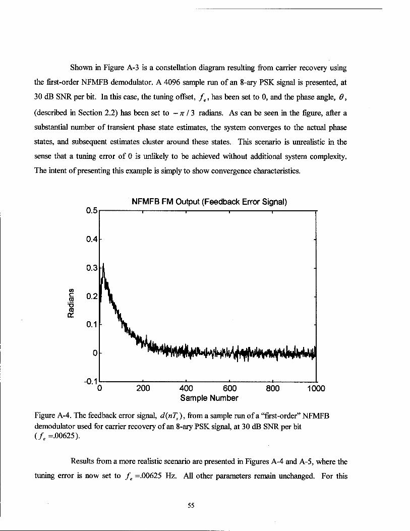
Shown in Figure A-3 is a constellation diagram resulting from carrier recovery using

the first-order NFMFB demodulator. A 4096 sample run of an 8-ary PSK signal is presented, at

30 dB SNR per bit. In this case, the tuning offset, fe, has been set to 0, and the phase angle, 0,

(described in Section 2.2) has been set to - n 13 radians. As can be seen in the figure, after a

substantial number of transient phase state estimates, the system converges to the actual phase

states, and subsequent estimates cluster around these states. This scenario is unrealistic in the

sense that a tuning error of 0 is unlikely to be achieved without additional system complexity.

The intent of presenting this example is simply to show convergence characteristics.

NFMFB FM Output (Feedback Error Signal)

CO c eg

CU DC

200 400 600 Sample Number

800 1000

Figure A-4. The feedback error signal, d(nTs), from a sample run of a "first-order" NFMFB demodulator used for carrier recovery of an 8-ary PSK signal, at 30 dB SNR per bit (/. =.00625).

Results from a more realistic scenario are presented in Figures A-4 and A-5, where the

tuning error is now set to fe =.00625 Hz. All other parameters remain unchanged. For this

55

example, in addition to presenting the constellation diagram, the feedback error signal, d(nTs),

(refer to Figure A-l) is also shown. As seen in Figure A-4, it has taken somewhere between 200

and 400 samples to converge to the expected nominal value of 0. It has also been observed that

(not unexpectedly) the system converges to phase states that are offset from the ideal states, by an

amount that is proportional to the tuning offset.

nfmfb-based Constellation Diagram 90

120\ "^60 ^^^m&KP"

• jfi' ■^*sN,^ / ^v ^V

™LJ*/ —s?\\\30 / J^s^f f "^■^X ^w x.^^^^ \ / / t^^^w g ^c \^^^ \ *\ \

L\ a / ^^V Jk^^ \ \ «li \

180 1* 1 / /

P\\ 1 P VSfc/ / / J 1 * J^\j/ III* 1

\ \5 V^^^^X ^yx/ a 1 21°\\N

"^1.

240^ ___^--^300

0

270

Figure A-5. A phase constellation diagram resulting from down-conversion to base-band using the NFMFB-recovered carrier frequency and phase. 4096 samples of an 8-ary PSK signal are shown, at 30 dB SNR per bit (/, =.00625). A "first-order" NFMFB was used.

A.1.2 Second-Order NFMFB Demodulator Example

Attention now turns toward an initial attempt to find a second-order NFMFB system,

which can be used in 8-ary PSK carrier recovery. In this example, the BPF remains as given in

Section A. 1.1, but the LPF is changed. The LPF is obtained by designing an initial filter, Hx(z).

The coefficients from this initial design, are then modified to include two integrators

(accumulators). This is accomplished by multiplying the initial LPF response, Hx(z), by the

56

response of a pair of integrators, i/2(z) = l/(l-z ) , and determining the resulting

denominator coefficients. (The integrator-pair transfer function is such that the numerator

coefficients remain unchanged.) For the example given, the initial "LPF" is Hx(z) = \ (i.e., a

bypass with no delay). A gain of £=.000001 (le-6) was chosen, which was experimentally found

to allow operation of the device for a fairly wide range of input SNR per bit values, indicating

stable operation. The description "second-order" is used to identify this configuration of the

device, because of the two additional integrators which have been combined with the initial LPF

design. (Strictly speaking, the system is of higher order in the sense that the BPF alone is of first

order, however, "second-order" will herein refer to the extra integrator-pair response. Note also

that the LPF filter is not of unity gain, once the integrators are included.) The filter, hB, shown in

the processing steps of Figure 2-2 b), was bypassed (not used) for this example.

nfmfb-based Constellation Diagram 90

180

330

270

Figure A-6. A phase constellation diagram resulting from down-conversion to base-band using the NFMFB-recovered carrier frequency and phase. 4096 samples of an 8-ary PSK signal are shown, at 30 dB SNR per bit (/, = 0). A "second-order" NFMFB was used.

57

With the tuning error set to 0, the error signal, d(nTs), (and therefore the carrier

phase estimate) exhibited an oscillatory behavior. As seen in Figure A-6, when using this carrier

estimate for subsequent processing, the phase state estimates would also oscillate back and forth

through the ideal phase states. The oscillation was rather low in frequency; about 1/2 cycle

occurred in the 4096 sample simulation. When fe was increased slightly (e.g., to .00003 Hz), the

oscillations increased in magnitude, closing the gaps observed between phase states in the

constellation diagram. (The omitted phase state was still apparent, up to fe s.0001 Hz.) Not

enough samples were observed to make an assertion regarding whether or not the error signal

amplitude remained constant.

A.1.3 Proportional Plus Integrator NFMFB Demodulator Example

The final example considered employs what is often referred to in the literature as a

"proportional plus integrator" loop filter. In this case, the LPF becomes

H r. l+fr-Qz-1 n

LPF\z)~ ,* -K2 ' (1-Z )

where x is a filter parameter. (Relating this filter to the example given in Section A. 1.2, it can be

derived by starting with the initial "LPF" design, Hl (z) = 1 + (x - l)z-1, and then combining this

initial response with the integrator pair response, H2 (z) = 1 / (1 - z"1 )2.) The filter, hB, shown in

the processing steps of Figure 2-2 b), is the same as that used for the FM discriminator-based

example given in Section 2.3.2. This filter is used to enhance performance of the NFMFB,

because in this example no BPF is used internal to the NFMFB (i.e., the BPF is bypassed). Also,

in this example, the closed-loop delay contributed by the NFMFB demodulator delay was

approximated as 0 samples.

Rather than engaging in fairly elaborate design procedures for choosing the gain, K,

and the filter parameter, JC, the work of [20] has been leveraged. In [20], the modulation index

5m = 2A/ IFS = 0.2315 is comparable to (and greater than) M=8 times the tuning error index,

Se = 2\fe\/Fs =.0125, used in this example. Thus, as in the reference, the gain is set to K = .765,

and the filter parameter is set to x = .285. The resulting constellation diagram is shown in Figure

58

A-7, for a tuning error of fe =.00625. It was observed that as the SNR per bit was decreased to

about 11 dB, the omitted phase state began to fill in, indicating excessive cycle skips. This was

true also for the FM discriminator-based example of Section 2.3.2. However, for the RNFMFB

example of Section 3.3.2, an omitted phase state did not begin to fill in until the SNR per bit was

decreased to about 8 dB.

nfmfb-based Constellation Diagram 90

150

180

210 330

270

Figure A-7. A phase constellation diagram resulting from down-conversion to base-band using the NFMFB-recovered carrier frequency and phase. 4096 samples of an 8-ary PSK signal are shown, at 30 dB SNR per bit (/, =.00625). A "proportional plus integrator" type NFMFB was used.

It was also observed in this example, that when fe was increased (doubled) to about .0125 Hz,

the system became "unstable" in the sense that random phase values between 0 and 2% were

present in the constellation diagram. This is as opposed to the RNFMFB example of Chapter 3,

which is tolerant of tuning errors as large as about .06 Hz, i.e., over nearly the entire Nyquist

band, -FJ{2M)<fe< +FSI (2M).

59

A.2 Additional Comments

The design philosophy used in this appendix has, once again, been the consideration

that time delay introduced by the synchronization device is a budgeted resource. Given this, the

post processing filter, h, shown in Figure 2-2 c) has been chosen to give an overall time delay, n0,

of 45 samples, for each of the examples presented. This filter is designed as an FIR filter with a

cut-off of .025 Hz relative to 1, using a Harming window.

60

Appendix B

Filter Response Plots

61

B.O Appendix Description

This appendix has been included to enhance the readability of the report. The

frequency responses of selected filters, from among those referred to within the main body and

Appendix A of the report, are provided. Each plot has an identifying figure caption which relates

the filter to the appropriate device component. The responses are grouped according to the

report section(s) in which the filters are referred to.

62

B.l Section 2.3.2 Filters

CO

a) | "c O) CO

-100 -0.2 0 0.2

Frequency (Hz) 0.4

b)

G 30 Q. E (0

>% TO 0 " <D D -10

20

10-

-0.4 -0.2 0 0.2 Frequency (Hz)

0.4

Figure B.l-1. Response of an order 50 FIR complex band-pass filter, hB, a Hanning window design with a cut-off of 0.075 Hz relative to 1 sample/sec; a) magnitude response, b) group delay.

a)

CD

"c

(0

-50

-100

b)

to

Q. ?0 b (0 (0 10 >. TO u 0) Q -10

_^i^, • 1 1

; 1 1 I V ;V 1/ \ A /-\i /v 0 0.1 0.2 0.3 0.4

Frequency (Hz)

. ! :

i i i 0.1 0.2 0.3

Frequency (Hz) 0.4

Figure B.l-2. Response of an order 40 FIR low-pass filter, h, a Hanning window design with a cut-off of 0.025 Hz relative to 1 sample/sec; a) magnitude response, b) group delay.

63

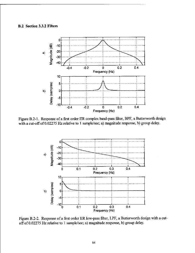
B.2 Section 3.3.2 Filters

a)

CD 2, <D

3

C O) CO

-0.4 -0.2 0 0.2 Frequency (Hz)

10

b)

10 a> Q. E (0 co

>» ro <D Q

-5

-10 -0.4 -0.2 0 0.2

Frequency (Hz) 0.4

Figure B.2-1. Response of a first order IIR complex band-pass filter, BPF, a Butterworth design with a cut-off of 0.02275 Hz relative to 1 sample/sec; a) magnitude response, b) group delay.

a)

CD TJ.

(D TJ 3 •f^ "c D) CD

0.1 0.2 0.3 Frequency (Hz)

b)

in $> Q. E (0 CO

ro <u D

10

5

0

-5

-10 0.1 0.2 0.3

Frequency (Hz) 0.4

Figure B.2-2. Response of a first order IIR low-pass filter, LPF, a Butterworth design with a cut- off of 0.02275 Hz relative to 1 sample/sec; a) magnitude response, b) group delay.

64

a)

b)

CO

<D TJ 3

C O) to 2

(0

Q. E (0

0) Q

-100

30

—~" ■ T 1 1 1

\ s [WWW lAAArt«;.

ra 0

-10

0.1 0.2 0.3 Frequency (Hz)

0.4

0.1 0.2 0.3 Frequency (Hz)

0.4

Figure B.2-3. Response of an order 60 FIR low-pass filter, h, a Harming window design with a cut-off of 0.0125 Hz relative to 1 sample/sec; a) magnitude response, b) group delay.

65

B.3 Section A.1.1 Filters

a)

-0.4 -0.2 0 0.2 Frequency(Hz)

b)

in a> Q. E <0 in

« Q

10

5

0

-5-

-10 -0.4 -0.2 0 0.2

Frequency (Hz) 0.4

Figure B.3-1. Response of a first order IIR complex band-pass filter, BPF, a Butterworth design with a cut-off of 0.02275 Hz relative to 1 sample/sec; a) magnitude response, b) group delay.

50

a) a> T3

C

as 2

-50 0.1 0.2 0.3

Frequency (Hz) 0.4

b)

0.1 0.2 0.3 Frequency (Hz)

0.4

Figure B.3-2. Response of a first order IIR low-pass filter, hx, a Butterworth design with a cut- off of 0.022115 Hz relative to 1 sample/sec; a) magnitude response, b) group delay.

66

a)

CO

CO T3 3

■*-»

C CJ) CO

b)

0.2 0.3 Frequency (Hz)

0.2 0.3 Frequency (Hz)

0.4

Figure B.3-2. Response of a "first order" IIR low-pass filter, LPF, a composite of a Butterworth design with a cut-off of 0.022115 Hz relative to 1 sample/sec, and an accumulator; a) magnitude response, b) group delay.

67

B.4 Section A.1.2 Filters

a)

CO TJ

TJ

C O) CO

-0.4 Frequency (Hz)

b)

jl> Q. E

Q

10

5

0

-5

-10 -0.4 -0.2 0 0.2

Frequency (Hz) 0.4

Figure B.4-1. Response of a first order IIR complex band-pass filter, BPF, a Butterworth design with a cut-off of 0.02275 Hz relative to 1 sample/sec; a) magnitude response, b) group delay.

a)

TJ

TJ 3 c (0

uu

50

0

1- ■ i 1 1

i i i i

0.1 0.2 0.3 Frequency (Hz)

0.4

b)

1/1 1 0) Q. E (0 0 m >» -1 (0 0) Q -2

0.1 0.2 0.3 Frequency (Hz)

0.4

Figure B.4-2. Response of the "second order" IIR low-pass filter, LPF, formed as an integrator (accumulator) pair; a) magnitude response, b) group delay.

68

B.5 Section A.1.3 Filters

-0.2 0 0.2 Frequency (Hz)

0.4

to 0)

30-

Q. 20|- b) ! ioh

m 0 Q -10

-0.4 -0.2 0 0.2 Frequency (Hz)

0.4

Figure B.5-1. Response of an order 50 FIR complex band-pass filter, hB, a Harming window design with a cut-off of 0.075 Hz relative to 1 sample/sec; a) magnitude response, b) group delay.

a)

CO

<D "o

'c ra CO

10

0

-10

-20

b)

to _g> Q. E CO

ro <u Q

( ) 0.1 0.2 0.3 0.4 Frequency (Hz)

o

0

-2

-4 i i i ■

0.1 0.2 0.3 Frequency (Hz)

0.4

Figure B.5-2. Response of a first order FIR filter, hx, with x = 0.285; a) magnitude response, b) group delay.

69

IUU 1 1 1 i

m T3

W) 0)

a)

(0 5

0 ■ i ' i <-

b)

(0

Q. E m Ä

5 03 Q

0.1 0.2 0.3 Frequency (Hz)

0.4

0.1 0.2 0.3 Frequency (Hz)

0.4

Figure B.5-3. Composite LPF response of the first order FIR filter of Figure B.5-2, and an integrator (accumulator) pair; a) magnitude response, b) group delay.

70

References

[I] J.L. Stensby, Phase-Locked Loops: Theory and Applications, CRC Press, Boca Raton, Fla., 1997.

[2] W.F. Egan, Phase-Lock Basics, Wiley, New York, 1998.

[3] A.V. Oppenheim, R.W. Schafer, Discrete-Time Signal Processing, Prentice-Hall, 1989.

[4] A. J. Noga, "Numerical FM Demodulation Enhancements," Rome Laboratory Technical Report RL-TR-96-91, June, 1996; "Performance Analysis and Simulation of a Class of Numerical Demodulation Techniques for Large Deviation FM Signals," Ph.D. Dissertation, Syracuse University, December 1995.

[5] P. Hasan, "PLL FM Demodulator Performance Under Gaussian Modulation " IEEE Transactions on Communications, Vol. 46, No. 4, April 1998.

[6] I. Galton, "Analog-Input Digital Phase-Locked Loops for Precise Frequency and Phase Demodulation," IEEE Transactions on Circuits and Systems-II: Analog and Digital Signal Processing, Vol. 42, No. 10, October 1995.

[7] S.H. Hao, Y. Puqiang, "A High Lock-In Speed Digital Phase-Locked Loop " IEEE Transactions on Communications, Vol. 39, No. 3, March 1991.

[8] M.E. Frerking, Digital Signal Processing in Communication Systems, Van Nostrand Reinhold, New York, 1994.

[9] J.G. Chaffee, "The Application of Negative Feedback to Frequency-Modulation Systems," Bell Systems Technical journal, Vol. 18, pp. 403-437, July 1939.

[10] J.A. Develet Jr., "Statistical Design and Performance of High-Sensitivity Frequency- Feedback Receivers," IEEE Transactions on Military Electronics, pp. 281-284, October 1963.

[II] L.M. Robinson, "Tanlock: A Phase-Lock Loop of Extended Tracking Capability," Proceedings IRE Conv. Military Electronics, February 1962.

[12] J.C. Lee, C.K. Un, "Performance Analysis of Digital Tanlock Loop," IEEE Transactions on Communications, Vol. COM-30, No. 10, pp. 2398-2411, October 1982.

[13] J.G. Proakis, Digital Communications, McGraw-Hill, 1989.

[14] S. Haykin, Communication Systems, 2nd Ed., John Wiley & Sons, New York, 1983.

71

[15] HJ. Kim, C.K. Un, J.C. Lee, "The N-Phase Digital Tanlock Loop for Tracking Suppressed- Carrier N-ary PSK Signals," IEEE Transactions on Communications, Vol. COM-33, No. 9, September 1985.

[16] W.D. Cho, C.K. Un, "On Improving the Performance of a Digital Tanlock Loop," Proceedings of the IEEE, Vol. 75, No. 4, April 1987.

[17] A.J. Viterbi, A.M. Viterbi, "Nonlinear Estimation of PSK-Modulated Carrier Phase with Application to Burst Digital Transmission," IEEE Transactions on Information Theory, IT-29, July 1983.

[18] L.H. Enloe, "Decreasing the Threshold in FM by Frequency Feedback," Proceedings IRE, Vol. 50, pp. 18-30, January 1962.

[19] S. Ono, T. Aoyama, M. Hagiwara, M. Nakagawa, "Implementation of a New Type DSP PLL Using High Performance DSP DSSP-1," Proceedings IEEE International Conference on Acoustics Speech and Signal Processing (ICASSP), pp. 2195-2198, April 1986.

[20] W. Rosenkranz, "Design and Optimization of a Digital FM Receiver Using DPLL Techniques," Proceedings IEEE International Conference on Acoustics Speech and Signal Processing (ICASSP), pp. 592-595, March 1985.

[21] M. Schwarz, W.R. Bennett, S. Stein, Communication Systems and Techniques, IEEE Press (Reprint), 1995.

[22] T.P. Krauss, L. Shure, J.N. Little, Signal Processing Toolbox User's Guide, for use with MATLAB™, The Mathworks, Inc., September 1995.

[23] D.T. Hess, "Equivalence of FM Threshold Extension Receivers," IEEE Transactions on Communication Technology, October 1968.

[24] J.L. Stensby, "Simple Real-Time Tracking Indicators for a Frequency Feedback Demodulator," Summer Faculty Research Program Final Report, Rome Laboratory, August 1997.

«U.S. GOVERNMENT PRINTING OFFICE: 1999-610-130-81141

72