Methods in biomedical text mining Raul Rodriguez-Esteban Submitted
144
Methods in biomedical text mining Raul Rodriguez-Esteban Submitted in partial fulfillment of the Requirements for the degree of Doctor of Philosophy in the Graduate School of Arts and Sciences COLUMBIA UNIVERSITY 2008
Transcript of Methods in biomedical text mining Raul Rodriguez-Esteban Submitted

Methods in biomedical text mining
Raul Rodriguez-Esteban
Submitted in partial fulfillment of theRequirements for the degree
of Doctor of Philosophyin the Graduate School of Arts and Sciences
COLUMBIA UNIVERSITY
2008

c©2008Raul Rodriguez-Esteban
All Rights Reserved
Abstract
Methods in biomedical text mining
Raul Rodriguez-Esteban
Methods to improve text mining of molecular biology interactions are needed to
capture a richer information space and qualify the quality of extraction. Simple
interaction models fail to describe contextual and confidence information that would
help with more fine-grained analyses. Herein a method is presented to streamline
curation of text-mined data and a way to improve text mining of biomedical terms
that can be adapted to other domains using different machine learning techniques.
These advances can be integrated into more powerful text-mining systems to meet
user demand and to further promote the adoption of text-mining tools. Additionally,
three studies on the nature of biomedical publications are presented: their novelty
hinges on the fact that each asks questions that had not been posed before. They
cover the phenomena of retraction, ways to improve the impact of research, and the
writing style used in biomedical literature. Retraction is a hot topic in recent times
but it has not been heeded in an analytical fashion. Measuring the impact of
scientific publications has brought heated debate on which are best at describing it.
We propose a method not to measure impact, but to improve it. Finally, we analyze
the influence of scientific writing style on the priming of its reader from a sensorial
point of view.

Contents
1 Overview of text mining of biomedical interactions 1
1.1 Text mining . . . . . . . . . . . . . . . . . . . . . . . . . . . . . . . . 1
1.2 Biomedical text mining . . . . . . . . . . . . . . . . . . . . . . . . . . 6
1.3 Interactions from text . . . . . . . . . . . . . . . . . . . . . . . . . . 8
1.3.1 GENIES . . . . . . . . . . . . . . . . . . . . . . . . . . . . . . 11
1.3.2 GeneWays . . . . . . . . . . . . . . . . . . . . . . . . . . . . . 12
1.4 Curation and evaluation . . . . . . . . . . . . . . . . . . . . . . . . . 13
2 Automatic curation of text-mined facts 18
2.1 Introduction . . . . . . . . . . . . . . . . . . . . . . . . . . . . . . . . 19
2.2 Approach . . . . . . . . . . . . . . . . . . . . . . . . . . . . . . . . . 20
2.3 Methods . . . . . . . . . . . . . . . . . . . . . . . . . . . . . . . . . . 21
2.3.1 Training data . . . . . . . . . . . . . . . . . . . . . . . . . . . 21
2.4 Mathematical background . . . . . . . . . . . . . . . . . . . . . . . . 26
2.4.1 Machine-learning algorithms . . . . . . . . . . . . . . . . . . . 26
2.4.2 Features used in our analysis . . . . . . . . . . . . . . . . . . . 38
2.4.3 Separating data into training and testing: Cross-validation . . 38
2.4.4 Comparison of methods: Receiver operating characteristic (ROC)
scores . . . . . . . . . . . . . . . . . . . . . . . . . . . . . . . 40
2.5 Results . . . . . . . . . . . . . . . . . . . . . . . . . . . . . . . . . . . 41
i

2.6 Discussion . . . . . . . . . . . . . . . . . . . . . . . . . . . . . . . . . 44
3 Overview of biomedical term recognition and classification 56
3.1 Introduction . . . . . . . . . . . . . . . . . . . . . . . . . . . . . . . . 56
3.1.1 Term recognition . . . . . . . . . . . . . . . . . . . . . . . . . 57
3.1.2 Named entity expressions . . . . . . . . . . . . . . . . . . . . 58
3.1.3 Term classification . . . . . . . . . . . . . . . . . . . . . . . . 59
3.1.4 Biomedical term recognition and classification . . . . . . . . . 62
3.2 Mathematical Background . . . . . . . . . . . . . . . . . . . . . . . . 72
3.2.1 Recognition and classification framework . . . . . . . . . . . . 72
3.2.2 Conditional random fields . . . . . . . . . . . . . . . . . . . . 74
4 Biomedical term recognition and classification using large corpora
and search engines 76
4.1 Introduction . . . . . . . . . . . . . . . . . . . . . . . . . . . . . . . . 76
4.2 Term recognition . . . . . . . . . . . . . . . . . . . . . . . . . . . . . 79
4.2.1 Text pre-processing and indexing . . . . . . . . . . . . . . . . 79
4.2.2 Syntactical model . . . . . . . . . . . . . . . . . . . . . . . . . 80
4.2.3 Term recognition process . . . . . . . . . . . . . . . . . . . . . 82
4.3 Term classification . . . . . . . . . . . . . . . . . . . . . . . . . . . . 85
4.3.1 Features . . . . . . . . . . . . . . . . . . . . . . . . . . . . . . 85
4.3.2 Local, regional, global: Word sense disambiguation . . . . . . 88
5 Six senses: the bleak sensory landscape of biomedical texts 91
6 A recipe for high impact 99
6.1 Ingredients of a scholarly study . . . . . . . . . . . . . . . . . . . . . 99
6.2 Information flow through publication-type niches . . . . . . . . . . . 101
6.3 Additional information . . . . . . . . . . . . . . . . . . . . . . . . . . 102
ii

6.3.1 Data . . . . . . . . . . . . . . . . . . . . . . . . . . . . . . . . 102
6.3.2 Analysis . . . . . . . . . . . . . . . . . . . . . . . . . . . . . . 102
7 How many scientific papers should be retracted? 105
7.1 Analyzing retraction patterns . . . . . . . . . . . . . . . . . . . . . . 105
7.2 Mathematical model to calculate the number of articles that should
have been retracted . . . . . . . . . . . . . . . . . . . . . . . . . . . . 108
7.3 Retraction rates are on the rise . . . . . . . . . . . . . . . . . . . . . 110
8 Future work and conclusions 113
8.1 Future work . . . . . . . . . . . . . . . . . . . . . . . . . . . . . . . . 113
8.2 Conclusion . . . . . . . . . . . . . . . . . . . . . . . . . . . . . . . . . 114
8.3 Papers that resulted from the work in this thesis . . . . . . . . . . . . 115
9 Bibliography 116
iii
List of Figures
2.1 Cocaine: the predicted accuracy of individual text-mined facts involving
semantic relation stimulate. . . . . . . . . . . . . . . . . . . . . . . . 19
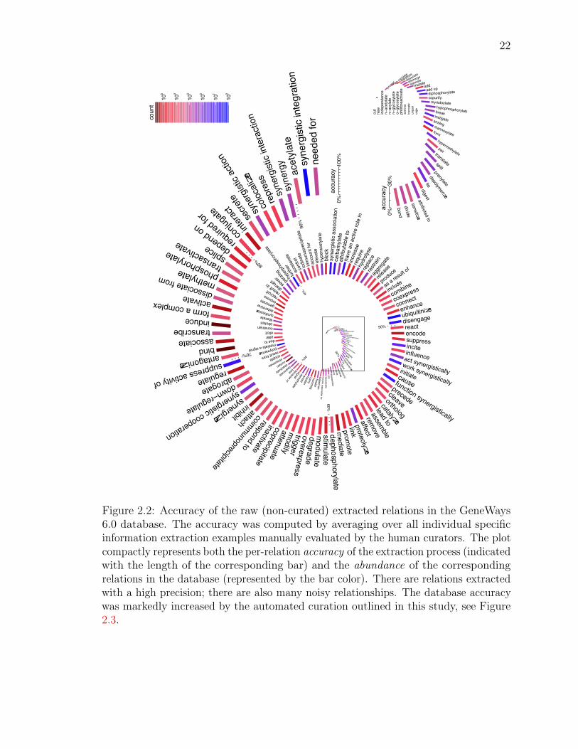
2.2 Accuracy of the raw (non-curated) extracted relations in the GeneWays
6.0 database. . . . . . . . . . . . . . . . . . . . . . . . . . . . . . . . 22
2.3 Accuracy and abundance of the extracted and automatically curated
relations. . . . . . . . . . . . . . . . . . . . . . . . . . . . . . . . . . . 23
2.4 Sentence Evaluation Tool . . . . . . . . . . . . . . . . . . . . . . . . . 25
2.5 The correlation matrix for the features used by the classification algo-
rithms. . . . . . . . . . . . . . . . . . . . . . . . . . . . . . . . . . . . 50
2.6 A hypothetical three-layered feed-forward neural network. . . . . . . . 51
2.7 Receiver-operating characteristic (ROC) curves for the classification
methods that we used in the present study. . . . . . . . . . . . . . . . 52
2.8 Correlation matrix. . . . . . . . . . . . . . . . . . . . . . . . . . . . . 53
2.9 Ranks of all classification methods used in this study in 10 cross-
validation experiments. . . . . . . . . . . . . . . . . . . . . . . . . . 54
2.10 Values of precision, recall and accuracy of the MaxEnt 2 classifier
plotted against the corresponding log-scores provided by the classifier. 55
5.1 Analysis of the frequencies of sensory words in six large corpora . . . 94
iv

6.1 Contributions of topic- and method-specific estimates of temperature
and novelty to a journal’s impact factor . . . . . . . . . . . . . . . . . 100
6.2 Number of articles, MeSH terms and chemical names mentioned in
PubMed since 1950 . . . . . . . . . . . . . . . . . . . . . . . . . . . . 102
7.1 Dataset, model and estimation of the number of flawed articles in
scientific literature . . . . . . . . . . . . . . . . . . . . . . . . . . . . 106
7.2 Number of articles and the percentage of articles retracted since 1950
as recorded in Medline. . . . . . . . . . . . . . . . . . . . . . . . . . . 112
v

List of Tables
1.1 Criteria for Evaluating Performance of NLP Systems. . . . . . . . . . 15
2.1 Sentence examples. . . . . . . . . . . . . . . . . . . . . . . . . . . . . 27
2.2 List of annotation choices available to the evaluators. . . . . . . . . . 28
2.3 Parameter values used for various SVM classifiers in this study. . . . 36
2.4 Machine learning methods used in this study and their implementations. 37
2.5 List of the features that we used in the present study. . . . . . . . . . 39
2.6 Comparison of the performance of human evaluators and of the MaxEnt
2 algorithm. . . . . . . . . . . . . . . . . . . . . . . . . . . . . . . . . 45
2.7 Comparison of human evaluators and a program that mimicked their
work. . . . . . . . . . . . . . . . . . . . . . . . . . . . . . . . . . . . . 46
2.8 ROCs . . . . . . . . . . . . . . . . . . . . . . . . . . . . . . . . . . . 49
3.1 Definition of token classes with differing semantic significance. . . . . 66
3.2 Morphologic feature values with examples. . . . . . . . . . . . . . . . 72
4.1 Examples of word labels for nested terms. . . . . . . . . . . . . . . . 84
4.2 Term classification performance. . . . . . . . . . . . . . . . . . . . . . 90
vi

Acknowledgements
I would like to thank Andrey Rzhetsky for the support and trust he has shown me
during my doctorate studies. His ideas inform this thesis and he shares a great deal of
the credit for what is written here. Murat Cokol led the work described in Chapters 6
and 7. Murat has been a continuous influence both in terms of advice and insight.
Ivan Iossifov collaborated in the studies reported in Chapters 2 and 7 and was helpful
in teaching me to navigate the GeneWays system. I also would like to thank other
members of the Rzhetsky lab: Igor Feldman, Chani Weinreb, Ilya Mayzus, Lixia Yao,
and Pauline Kra.
vii

To my family.
viii

1
Chapter 1
Overview of text mining of
biomedical interactions
The purpose of this introduction is to give a historical overview and background to
the project of automatic curation of text-mined data described in Chapter 2. This
introduction describes the beginnings of text mining as a discipline and its arrival to
the biomedical domain. It also describes the first interaction text mining projects,
which precede and set a path to the development of GeneWays. This introduction is
necessary to understand the architectural and structural choices made for the design
of GeneWays. Finally, this introduction reviews the different efforts made in
evaluating text-mined interaction data before the automatic curation project was
developed. The aim is not only to contextualize the state of the art and decisions
made during the project but also to present the basis on which it stood and the
challenges it faced.
1.1 Text mining
The field of text mining is a relatively new discipline born of the knowledge discovery
in databases (KDD) and data mining (DM) community. As it is often the case when

2
a discipline is born, it borrowed techniques and approaches from similar, more
established fields before establishing its own identity 1.
Alessandro Zanasi claims that the first time he heard the term “text mining” was
when it was spoken by Charles Huot in 1994, during the IBM-ECAM (European
Centre for Applied Mathematics) [1] workshop in Paris. Whether it was used with
the same meaning that it has today, in the context of applications such as
information extraction [2] or document classification [3], is unclear. In 1995 and 1996,
Ronen Feldman and colleagues offered the first contributions to the field that can be
called text mining with more certainty [4, 5, 6], originally called knowledge discovery
in text (KDT). The word mining was soon introduced in 1996 in the context of KDT,
followed by the coinage of the name “text mining”, a variation of the name data
mining. By 1997 the expression text mining had become an accepted name for the
new discipline. The new discipline quickly spawned courses, workshops, and books
and opened new avenues of research and notable subfields, such as web text mining
(1998) and biomedical text mining (1998). Text mining brought together researchers
from the KDD and DM communities and from the fields of natural language
processing (NLP), automatic knowledge acquisition, information retrieval, and
information extraction, to name a few. Text mining became the predominant name
for the discipline, widely replacing other names such as KDT, KDT and text mining,
textual data mining, and text data mining. That some of these names are still in use
reflects not only a stylistic choice but also, in some cases, differences in understanding
of aims, scope, and methods.
Marti Hearst [7] was one of the first to summarize the state of the nascent discipline
in 1999, attempting to define its scope with respect to other fields such as data
mining, computational linguistics, or information retrieval. Hearst stressed that the
defining quality of text mining is that its goal is to discover novel information, unlike
1Think of the first cars having the shape of horse carts, or the first films looking like theater plays
3
fields such as information retrieval and data mining. In this respect, text mining is
indebted to literature-based discovery, a field championed by Don Swanson beginning
with his seminal paper in 1986, “Undiscovered public knowledge” [8, 9].
Literature-based discovery was intended to be a systematic search for pieces of
knowledge that could be combined to create a novel discovery. Originally,
literature-based discovery was largely a non-automated process. Swanson recalled
stumbling onto the idea through a serendipitous finding of two unrelated articles that
could be combined to answer a question that no other single article answered. His
acceptance speech upon receiving the American Society for Information Science and
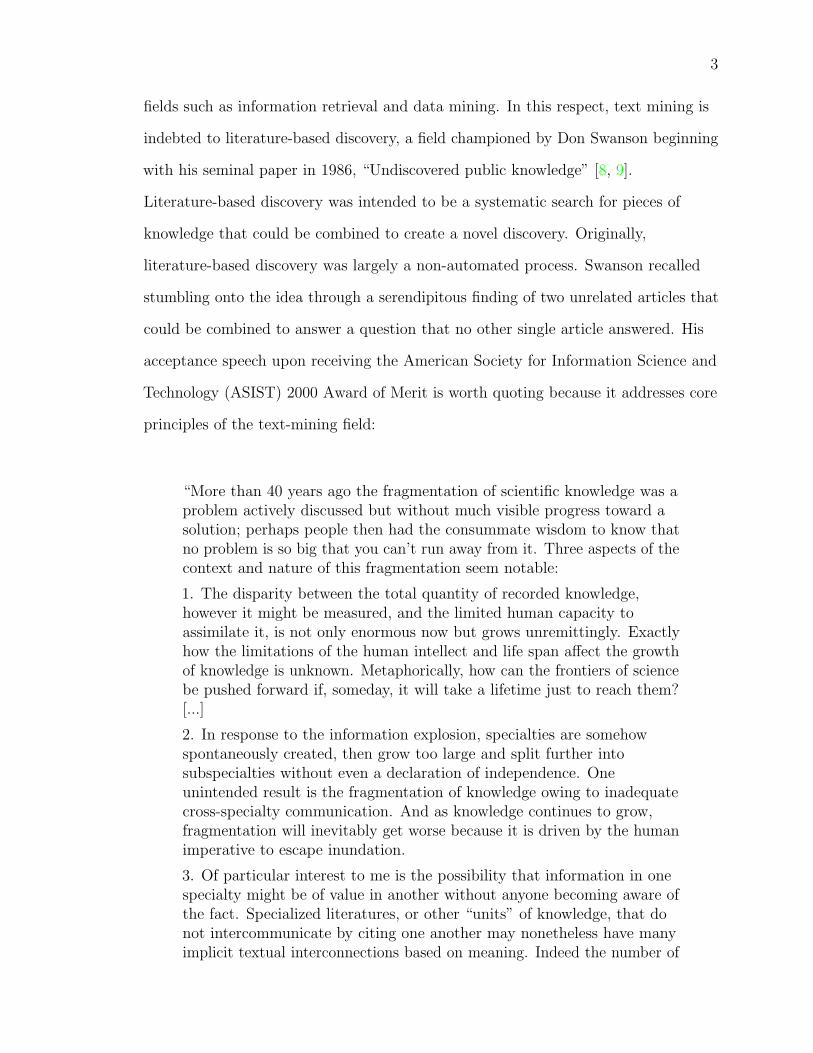
Technology (ASIST) 2000 Award of Merit is worth quoting because it addresses core
principles of the text-mining field:
“More than 40 years ago the fragmentation of scientific knowledge was aproblem actively discussed but without much visible progress toward asolution; perhaps people then had the consummate wisdom to know thatno problem is so big that you can’t run away from it. Three aspects of thecontext and nature of this fragmentation seem notable:
1. The disparity between the total quantity of recorded knowledge,however it might be measured, and the limited human capacity toassimilate it, is not only enormous now but grows unremittingly. Exactlyhow the limitations of the human intellect and life span affect the growthof knowledge is unknown. Metaphorically, how can the frontiers of sciencebe pushed forward if, someday, it will take a lifetime just to reach them?[...]
2. In response to the information explosion, specialties are somehowspontaneously created, then grow too large and split further intosubspecialties without even a declaration of independence. Oneunintended result is the fragmentation of knowledge owing to inadequatecross-specialty communication. And as knowledge continues to grow,fragmentation will inevitably get worse because it is driven by the humanimperative to escape inundation.
3. Of particular interest to me is the possibility that information in onespecialty might be of value in another without anyone becoming aware ofthe fact. Specialized literatures, or other “units” of knowledge, that donot intercommunicate by citing one another may nonetheless have manyimplicit textual interconnections based on meaning. Indeed the number of
4
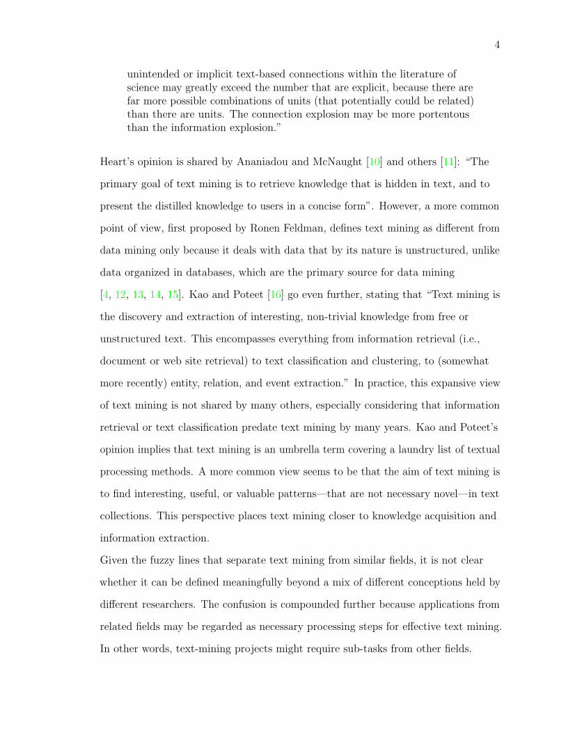
unintended or implicit text-based connections within the literature ofscience may greatly exceed the number that are explicit, because there arefar more possible combinations of units (that potentially could be related)than there are units. The connection explosion may be more portentousthan the information explosion.”
Heart’s opinion is shared by Ananiadou and McNaught [10] and others [11]: “The
primary goal of text mining is to retrieve knowledge that is hidden in text, and to
present the distilled knowledge to users in a concise form”. However, a more common
point of view, first proposed by Ronen Feldman, defines text mining as different from
data mining only because it deals with data that by its nature is unstructured, unlike
data organized in databases, which are the primary source for data mining
[4, 12, 13, 14, 15]. Kao and Poteet [16] go even further, stating that “Text mining is
the discovery and extraction of interesting, non-trivial knowledge from free or
unstructured text. This encompasses everything from information retrieval (i.e.,
document or web site retrieval) to text classification and clustering, to (somewhat
more recently) entity, relation, and event extraction.” In practice, this expansive view
of text mining is not shared by many others, especially considering that information
retrieval or text classification predate text mining by many years. Kao and Poteet’s
opinion implies that text mining is an umbrella term covering a laundry list of textual
processing methods. A more common view seems to be that the aim of text mining is
to find interesting, useful, or valuable patterns—that are not necessary novel—in text
collections. This perspective places text mining closer to knowledge acquisition and
information extraction.
Given the fuzzy lines that separate text mining from similar fields, it is not clear
whether it can be defined meaningfully beyond a mix of different conceptions held by
different researchers. The confusion is compounded further because applications from
related fields may be regarded as necessary processing steps for effective text mining.
In other words, text-mining projects might require sub-tasks from other fields.
5
Therefore, text mining in some contexts might be used for the sole purpose of
indicating the scientific agenda in which the study should be considered, not for
defining the task itself as “text mining”. Furthermore, as other fields have built on
advances in text mining, text mining also has become an intermediate step in projects
of different nature.
Related disciplines such as semantic analysis, text analysis, information retrieval,
information extraction, and knowledge acquisition have a much older pedigree within
the computation and information sciences than does text mining. Like text mining,
they derive from activities that originally could be handled by human intellect and
rudimentary record-keeping but became more complex with the progressive
accumulation of knowledge and information. Fielden [17] plotted the evolution of the
size of information repositories over the course of human history, showing an
exponential growth in the last decades. More comprehensively, Peter Lyman and Hal
Varian led a study designed to estimate the quantity of information produced
worldwide every year [18, 19]; they estimated a grand total of 5 exabytes2 , or 800
megabytes per person per year, of which 92% were in magnetic storage. Printed text
represented 33 terabytes, whereas the “surface internet” accounted for 167 terabytes
and the “deep internet” (or database, dynamically-generated pages) for about 92
petabytes). This unparalleled growth has been accompanied by extraordinary
improvements in the devices and methods in the different computation and
information sciences. Text mining, a late arrival, has the advantage of drawing from
an extensive set of diverse techniques developed not only in the related disciplines,
but also in other fields such as machine learning, artificial intelligence, probabilistic
2Clearly, not all those bytes are useful. The problem is not confined to sorting large amounts ofdata but also to seeing through the “information pollution” that clouds data analysis. It may beworth quoting T. S. Eliot again:
“Where is the wisdom we have lost in knowledge? Where is the knowledge we have lostin information?”

6
analysis, statistics, pattern recognition, data management, and information theory.
While other disciplines, like information retrieval, fledged out before the current
pervasive use and availability of electronic text, text mining was born in a seemingly
limitless and growing frontier of resources and opportunities. Text miners, in turn,
have acted like they have a hammer and see a nail in everything. Perhaps this is the
best explanation for the success of text mining: Applications have driven its evolution
[1].
Given the fragmentary state of the field, it is not surprising that there is not currently
a journal that specializes in text mining. The door is open for further transformation
of the text-mining domain, whether in terms of its buzz or its consolidation in the
spectrum of computation and information sciences.
1.2 Biomedical text mining
The first attempts at text mining of the biomedical literature date back to 1998. As
explained in Section 1.1, the label “text mining” may have consumed some areas that
formerly went by a different name, such as knowledge acquisition and information
extraction. Text mining builds on previous informatics and computational work on
semantic analysis, dictionary creation, knowledge acquisition, classification, etc. Its
application to the biomedical realm is a natural extension given the existing
opportunities: exponential growth of the literature—both in size and in electronic
availability—; the gradual shift to electronic medical records; the on-going work in
annotated resources (e.g., Gene Ontology (GO), Online Mendelian Inheritance in
Man (OMIM), Swissprot); and the increasing need for integration between
information sources of disparate origin, also known as integromics [20]. The internet
is the main engine that has fuelled this growth. Even though computers and
electronic communications long predated the internet, it is the internet that has
7
crystallized change because it has dramatically lowered the cost of information access
and exchange and brought to the social forefront the challenges and opportunities of
biomedical electronic information (e.g., the Health Insurance Portability and
Accountability Act of 1996; the Open Access movement).
Integromics is proving to be of crucial importance in current developments as more
data are becoming available in different formats in electronic and on-line form,
including supplementary information tables, genome linkage maps, DNA sequences,
taxonomies, ontologies, hospital medical records, and semi-structured forms (e.g.,
questionnaires), etc. An example is Medline [21], an exponentially growing biomedical
bibliography that accounts for upwards of 16 million articles. In many cases, Medline
has references to full-text articles that may be retrieved with the appropriate licenses.
However, information related to those articles, like on-line repositories or
supplementary text and tables, is harder to access. Medline’s growth can be
considered even more dramatic if we include the “deep Medline” trove of additional
resources that are ready for mining.
Biomedical text miners may claim the superiority of text-mined data over other
resources, especially over manually curated data. Text mining casts a wide net over
the biomedical spectrum, allowing individual researchers to deal with Swanson’s three
arguments for library knowledge discovery (see Section 1.1). The resulting catch is
larger than can typically be gathered manually. As of October 2007, the hand-curated
Database of Interacting Proteins (DIP, [22]) held 56,186 interactions. Perhaps the
most extensive effort in manual literature-derived extraction of interactions is
BioGRID [23], with 70,000 interactions. In comparison, some text-mining interaction
repositories hold over half a million interactions (see Section 1.3.2). The NCBI Gene
Expression Omnibus repository of microarray expression datasets contains about half
a billion data samples [24]. Hence, text-mined biomedical data has a place within the
suite of tools available to biomedical informaticians and researchers. For the examples
8
given, this place lies somewhere between high throughput methods and manually
hand-curated sets, each with its own niche applications. The challenge for biomedical
text mining is to assert its usefulness both for acquiring information with quality that
approaches (or surpasses) hand-curated data and for reaching the widest coverage for
system-wide analysis (e.g., characterizing complex diseases [25]).
Some applications in biomedical text mining have mirrored those of text mining at
large, like document classification, data integration, literature-based discovery, and
literature analysis (e.g., scientific trends and emerging topics [26]). Others have been
more specific to biomedicine, such as biomedical annotation, phenome/phenotype
analysis, public health informatics (e.g., news analysis [27], hospital rankings [28]),
clinical informatics, and nursing informatics. The most flourishing areas, however,
may be loosely defined as those closely linked to systems biology [29, 30] and medical
text mining. The former deals with such topics as biomedical interaction extraction,
functional analysis, or genome annotation among others (see a list of main tools and
repositories in [31]). The latter deals with the range of narratives found in the textual
supports associated with clinical settings, from the ICU bedside to the clinical trials
desk. Biomedical text-mining articles are published mostly in journals and
conferences in biomedical informatics and computational biology, and sometimes in
non-informatics journals like Genome Biology.
1.3 Interactions from text
Systems biology has been a hotbed for developments in biomedical text mining, as
mentioned in Section 1.2. One of the focuses has been on interactions between
different types of molecules, especially proteins (i.e., PPI, protein-protein
interactions). The success of PPI can be seen in its application for integrative studies,
the popularity of its tools, and its use as support for public databases like DIP [32],
9
MINT [33], and BIND [34]. The interactions, taken from a functional genomics point
of view, range from physical (e.g. protein binding) to indirect (e.g., proteins in the
same pathway but not physically interacting) interactions to other phenomena, such
as co-expression. The interaction triplet has been an important text-mining
interaction model since its inception. This triplet consists of the two elements that
are involved in the interaction and the verb or action word that relates them. In the
GeneWays ontology [35], the elements of the triplet are called the upstream term,
downstream term, and action. Triplets usually are taken from single sentences. For
example, in the sentence “Gene A activates gene B.”, “gene A” is the upstream term,
“gene B” is the downstream term, and “activate” is the action. This model was first
introduced in a preliminary study by Sekimizu and colleagues [36], in which they
sought verbs that could characterize gene-gene interactions. Rindflesch and colleagues
[37] experimented with sentences that included the verb “bind”.
An alternative model to triplets is used in co-occurrence studies. Stapley and Benoit
[38], for example, used co-occurrence in a study of selected PubMed abstracts,
followed later by the larger-scale project PubGene [39]. With this method,
interactions are inferred from co-occurrence statistics of two terms in documents. If
the terms co-occur in text more often than could be expected, it is argued, that there
is basis to suggest that they may be related. Co-occurrence is a statistical method
used early in information retrieval. It has been used in different types of analyses but,
due to its limitations, it has not become a method of general use in the text mining of
interactions. Co-occurrence, for example, is of limited help in distinguishing
interactions of very low frequency. Another drawback of this method is that the
nature of the interaction is lost.
Some of the problems that biomedical interaction extraction entails are common to
biomedical texts at large, such as extensive and open-ended vocabulary, erratic
abbreviations, word sense ambiguity, and convoluted sentences. Others are more

10
specific. For example, negative particles or words with negative meaning may
completely change the meaning of an interaction, e.g., “We could not find any
interaction between gene A and gene B” (for a study on a negative interactome, see
[40]). Anaphora is another challenging problem that rarely is tackled (although see
[41]). Anaphora refers to situations in which the name of an object is elided,
generally because a pronoun is used to avoid repetition, e.g. “It activates gene B.”
The challenge is to identify the object to which “it” refers. More generally speaking,
biomedical interaction extraction faces the hurdles of the different pre-processing
steps plus the complexity of identifying the interactions themselves.
Blaschke and colleagues [42] proposed an early rule-based model for interaction
extraction that tried to capture a simple lexical pattern in sentences: “protein A -
action - protein B”. The names of the proteins and the action were identified using
controlled vocabularies. Thomas and colleagues [43] used syntactic instead of lexical
patterns (an example of a syntactic pattern is noun phrase - verb - noun phrase) to
find triplet candidates that were then narrowed down through a hand-crafted scoring
system. The syntactic analysis performed was of the shallow type, which can be done
more quickly than deep or full parsing and it only identifies units at the syntagma
level of the sentence (e.g., noun phrases and verb phrases). Proux and colleagues [44]
developed the approaches used in [43] and [42] by using first syntactic parsing and
then applying lexical patterns to find interactions. Similar approaches were explored
by [45] and [46], although they did not report to have fully implemented them.
Blaschke and colleagues created a generalized pattern approach, calling these patterns
“frames” [47, 48]. Frames are flexible patterns that may include additional information
to enrich the analysis (e.g., the distance in words between the interaction terms of the
sentence). Park and colleagues [49] and Yakushiji and colleagues [50] went further by
including full syntactic parsing in their systems. Full parsing allows for categorization
of all syntactic dependencies among the words of a sentence. The GENIES parser [51]

11
was born within this context of incipient improvement and tests of new approaches.
1.3.1 GENIES
GENIES [51] evolved from MedLee [52], a medical natural-language processing
application in use at the Clinical Information System (CIS) of New York Presbyterian
Hospital. MedLee was inspired by the sub-language theory of Zellig Harris [53], its
main trait was its semantic grammar, which combined grammatical patterns and
lexical information to capture different structures. In contrast to other semantic
grammar systems, pattern matching in MedLee must be exact. Only the sequences
that conform precisely to a specific pattern both grammatically and semantically are
considered. This approach was chosen to extract information both efficiently and
reliably.
The MedLee processing pipeline consists of several parts:
• Pre-processor: The text is formatted for manipulation and then analyzed
lexically using a lexicon.
• Parser: The text is analyzed grammatically (deep grammatical parsing). If the
grammatical parsing fails there is an error recovery step to break the sentences
into segments more amenable to manipulation. These segments then are
analyzed grammatically.
• Phrase recognition: Terms that are adjacent and that could form a phrase are
combined together (e.g., “chest” followed by “pain” is combined into “chest
pain”).
• Encoder: Terms are mapped to a controlled vocabulary.
GENIES uses the pre-processor and parser modules from MedLee adapting them to
the systems biology domain. The semantic categories in GENIES (e.g., amino acid,

12
cell, complex, domain, DNA region, etc.) mostly differ from those in MedLee (e.g.,
body location, finding, device, disease, procedure, etc.) although a few overlap (e.g.,
certainty, connective). The grammar rules of the parser module were adapted to the
new semantic categories. An important difference from Harris’s sub-language theory
is that the patterns were constructed manually from perceived patterns of interest in
biomedical texts, whereas Harris proposed using statistical methods. Furthermore,
GENIES receives its input from a term tagger that uses BLAST [54] pattern-matching
algorithm to recognize a term even if it is written with slight variations [55].
1.3.2 GeneWays
GeneWays [35] is a system designed for the automatic extraction of signal
transduction pathways, although, more broadly, it can be characterized as a system
designed to capture gene, protein, and small molecule interactions. GeneWays 6.0
stores 4,035,759 relationships (of which 2,652,916 are unique) from 232,265 full-length
articles published between 1994 and 2004 in 78 journals, it is the largest repository in
its class. GeneWays’s major strength is its use of an extensive collection of full-text
articles. Other prime examples of large-scale interaction repositories are:
1. iHOP [56], with 30,000 different genes and half a million sentences (and 500,000
website hits per month [57])
2. PubGene [39], with 1,087,757 relationships (139,756 unique) and 13,712 genes
3. PRIME, with 920,000 unique protein interactions [58]
At its core, GeneWays is GENIES, and it has built around GENIES the following set
of modules for extra processing and display:
• On the input side, a module fetches on-line, full-text articles and stores them in
a repository.
13
• The term tagging module was improved by the addition of a term
classifier/disambiguator [59].
• On the output side, a Simplifier module transforms the output from GENIES
into simple triplet relations (e.g., “interleukin-2 binds interleukin-2 receptor”)
following the GeneWays ontology [60], which is more suitable for analysis of
regulatory networks.
• The output from the simplifier is stored in the Interaction Knowledge Base, a
relational database.
• The knowledge base and other data elements product of the GeneWays pipeline
(e.g., the terms extracted), can be displayed using a graphical tool called
CUtenet that allows for network plotting as well as other data presentation
formats.
Hence, GeneWays covers a number of steps including retrieval, processing, storage,
and display, that allow end users to select their information of interest. GeneWays
data can be used in multiple ways to furthering research of different issues in systems
biology, text mining, and scientometrics [61, 62, 63, 64, 65].
1.4 Curation and evaluation
The idea of automatically curating a text-mined knowledge base was first proposed in
the original GeneWays paper as an extra module called the AI curator. It was
presented in the following way [35]:
“Note that the automatically generated knowledge base is of necessitynoisy: the GeneWays system extracts some percentage of statementsincorrectly, and, even among correctly extracted statements, we shouldexpect redundancy and contradictions. Therefore, the database requires
14
curation, a process in which the original statements are annotated withstatements regarding confidence in the corresponding information. Thetraditional way to perform such curation is through manual labor ofhuman experts—a monumental task even for the database at its currentsize of roughly 3 million redundant statements extracted from 150,000articles. To reduce the manual work, we are implementing a Curatormodule that would allow GeneWays to compute the estimates ofreliability automatically.”
Curation is considered a step in the process of ascertaining the truth of certain facts,
especially for the scientist who is confronted with multiple, sometimes conflicting,
pieces of information and who needs to make decisions within the knowledge pocket
of her particular scientific specialization [66, 63, 65]. Curation also provides a way to
assign a value to our degree of confidence about a fact within a continuous scale of
truth. The value of truth assigned is an attempt to represent our limited ability to
completely understand a text, or even the limited ability of the writer to express what
she wants to say.
Evaluation is a central part of curation. Systems biology studies face the difficult task
of measuring recall in a broad and intricate search space combined with the
limitations of manual evaluation of precision. Many evaluations in the literature,
including many of those cited herein, were not described in detail, which makes it
hard to establish their characteristics. Often, they entail in-house evaluations in which
unnamed experts follow protocols that are not detailed. This is understandable from
the point of view that, in most cases, evaluations are considered a necessary, but not
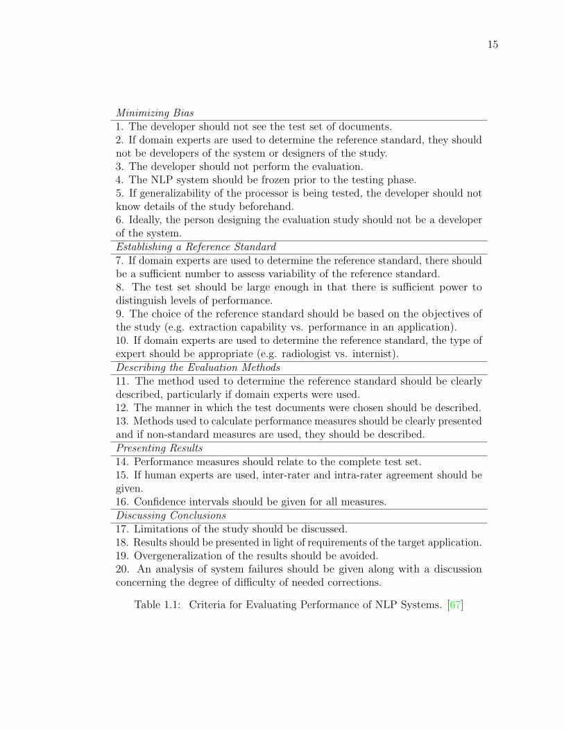
central, contribution. Friedman and Hripcsak [67] exposed a number of pitfalls in the
task of evaluating NLP systems and defined 20 criteria to avoid them (see Table 1.4).
In Sekimizu and colleagues’ seminal paper [36], two experts evaluated a random set of
several hundred assertions with typical interaction verb connectors (activate, interact,
encode, regulate, prevent, contain, inhibit, or bind). The researchers identified a
different precision associated with each action type, a phenomenon also noted by Ono
and colleagues [68]. Rindflesch and colleagues [37] used a test set of manually
15
Minimizing Bias1. The developer should not see the test set of documents.2. If domain experts are used to determine the reference standard, they shouldnot be developers of the system or designers of the study.3. The developer should not perform the evaluation.4. The NLP system should be frozen prior to the testing phase.5. If generalizability of the processor is being tested, the developer should notknow details of the study beforehand.6. Ideally, the person designing the evaluation study should not be a developerof the system.Establishing a Reference Standard7. If domain experts are used to determine the reference standard, there shouldbe a sufficient number to assess variability of the reference standard.8. The test set should be large enough in that there is sufficient power todistinguish levels of performance.9. The choice of the reference standard should be based on the objectives ofthe study (e.g. extraction capability vs. performance in an application).10. If domain experts are used to determine the reference standard, the type ofexpert should be appropriate (e.g. radiologist vs. internist).Describing the Evaluation Methods11. The method used to determine the reference standard should be clearlydescribed, particularly if domain experts were used.12. The manner in which the test documents were chosen should be described.13. Methods used to calculate performance measures should be clearly presentedand if non-standard measures are used, they should be described.Presenting Results14. Performance measures should relate to the complete test set.15. If human experts are used, inter-rater and intra-rater agreement should begiven.16. Confidence intervals should be given for all measures.Discussing Conclusions17. Limitations of the study should be discussed.18. Results should be presented in light of requirements of the target application.19. Overgeneralization of the results should be avoided.20. An analysis of system failures should be given along with a discussionconcerning the degree of difficulty of needed corrections.
Table 1.1: Criteria for Evaluating Performance of NLP Systems. [67]

16
annotated sentences as gold standard to evaluate their application’s ability to identify
the action type “bind”. Blaschke and colleagues [42] used two networks of known
protein interactions as prediction targets for their system. They trained their system
with selected Medline abstracts that included information about these networks, and
then tested to see whether it had learned the network correctly. Stapley and Benoit
[38] focused on relationships extracted from Medline documents with the MeSH term
“DNA repair”. Reducing the search space to a specific domain eliminated the need to
choose random documents from a repository (e.g. Medline), as was done initially in
[36]. A limited evaluation, however, reduced the generalizability of the results.
Thomas and colleagues [43] proposed, but did not implement, a scoring system to
measure the level of certainty that a relationship has been well extracted by using as
a template a pattern of co-occurrence. The scoring system would assign a score to
each template based on three factors:
1. Textual context (i.e., neighborhood of words and sentences).
2. Degree of confidence that the term is a protein.
3. Frequency in which the relationship appears.
However, they implemented a score based on the degree of likelihood that the terms
of a given template are proper names. A template was considered more reliable if it
identified relationships whose terms are proper names. Their rationale was that
proper names are more likely to indicate protein names. Their scoring point scale (or
scoring strategy) was, otherwise, arbitrary and it was used to make a preliminary
filter of results. Proux and colleagues [44] used 200 sentences pre-evaluated by experts
(evaluated as correct, incorrect, or undecided) as evaluation. This method became the
most commonly used. Blaschke and Valencia [47] used word distance between terms
and actions to yield estimated likelihoods of precision. They used a heuristic
approach to compute probabilities for different word distances in order to give each
17
result an estimated precision likelihood. Jenssen and colleagues [39] used actual
micro-array expression data as a gold-standard for their gene co-occurrence text
mining. The relationships found were compared to micro-array co-expression results.
In-house expert evaluation has been the most common method both for result
evaluation and for gold-standard generation. Efforts like the Critical Assessment of
Information Extraction (BioCreAtIvE) [69], which followed the lead of the successful
Critical Assessment of PRediction of Interactions (CAPRI) [70], have raised
awareness in the biomedical text-mining community about the use of common
evaluation test sets and standards. Daraselia and colleagues [71] performed a manual
evaluation supplemented by cross-comparisons with the DIP and BIND databases.
These databases are manually curated repositories that use co-occurrences as a
pre-screening filter. Chen and Sharp [72] went further in this approach and used a set
of interactions selected from DIP as a prediction target for their system. Hakenberg
and colleagues [73] created evaluation sets from articles referenced in DIP and the
annotated BioCreAtIvE corpus. Koike and colleagues [58] used abstracts from GO
term annotations. The main strength of evaluation techniques that use publicly
available, manually curated corpora is that comparisons can be made between
evaluation results of different applications.
The state of evaluation in the text mining of biomedical interactions sets the stage for
the automatic curation project in Chapter 2, the aim of which is to go beyond
existing evaluation schemes as so far described.
18
Chapter 2
Automatic curation of text-mined
facts
...he will throughly purge his floor, and gather his wheat into the garner;
but he will burn up the chaff with unquenchable fire.
Matthew 3:12 [74]
Synopsis
Current automated approaches for extracting biologically important facts from
scientific articles are imperfect: while being capable of efficient, fast and inexpensive
analysis of enormous quantities of scientific prose, they make errors. In order to
emulate the human experts evaluating the quality of the automatically extracted facts,
we have developed an artificial intelligence program (“a robotic curator”) that closely
approaches human experts in the quality of distinguishing the correctly extracted facts
from the incorrectly extracted ones.

19
Figure 2.1: Cocaine: the predicted accuracy of individual text-mined facts involvingsemantic relation stimulate. Each directed arc from an entity A to an entity B in thisfigure should be interpreted as a statement “A stimulates B”, where, for example, Ais cocaine and B is progesterone. The predicted accuracy of individual statementsis indicated both in color and in width of the corresponding arc. Note that, forexample, the relation between cocaine and progesterone was derived from multiplesentences, and different instances of extraction output had markedly different accuracy.Altogether we collected 3, 910 individual facts involving cocaine. So long as the samefact can be repeated in different sentences, only 1, 820 facts out of 3, 910 were unique.The facts cover 80 distinct semantic relations, out of which stimulate is just oneexample.
2.1 Introduction
Information extraction uses computer-aided methods to recover and structure
meaning that is locked in natural-language texts. The assertions uncovered in this
way are amenable to computational processing that approximates human reasoning.
In the special case of biomedical applications, the texts are represented by books and
research articles, and the extracted meaning comprises diverse classes of facts, such as
relations between molecules, cells, anatomical structures, and maladies.
Unfortunately, the current tools of information extraction produce imperfect, noisy
20
results. Although even imperfect results are useful, it is highly desirable for most
applications to have the ability to rank the text-derived facts by the confidence in the
quality of their extraction (as we did for relations involving cocaine, see Figure 2.1).
We focus on automatically extracted statements about molecular interactions, such as
small molecule A binds protein B, protein B activates gene C, or protein D
phosphorylates small molecule E. (In the following description we refer to phrases that
represent biological entities (such as small molecule A, protein B, and gene C ) as
terms, and to biological relations between these entities (such as activate or
phosphorylate) as relations or verbs.)
Several earlier studies have examined aspects of evaluating the quality of text-mined
facts, as explained in Section 1.4. For example, Sekimizu et al. and Ono et al.
attempted to attribute different confidence values to different verbs that are
associated with extracted relations, such as activate, regulate, and inhibit [36, 68].
Thomas et al. proposed to attach a quality value to each extracted statement about
molecular interactions [43], although the researchers did not implement the suggested
scoring system in practice. In an independent study [47], Blaschke and Valencia used
word-distances between biological terms in a given sentence as an indicator of the
precision of extracted facts. In our present analysis we applied several
machine-learning techniques to a large training set of 98, 679 manually evaluated
examples (pairs of extracted facts and corresponding sentences) to design a tool that
mimics the work of a human curator who manually cleans the output of an
information-extraction program.
2.2 Approach
Our goal is to design a tool that can be used with any information-extraction system
developed for molecular biology. In this study, our training data came from the
21
GeneWays project (specifically, GeneWays 6.0 database, [51, 35]) and thus our
approach is biased toward relationships that are captured by that specific system1.
We believe that the spectrum of relationships represented in the GeneWays ontology
is sufficiently broad that our results will prove useful for other information-extraction
projects.
Our approach followed the path of supervised machine-learning. First, we generated a
large training set of facts that were originally gathered by our information-extraction
system, and then manually labeled as “correct” or “incorrect” by a team of human
curators. Second, we used a battery of machine-learning tools to imitate
computationally the work of the human evaluators. Third, we split the training set
into ten parts, so that we could evaluate the significance of performance differences
among the several competing machine-learning approaches.
2.3 Methods
2.3.1 Training data
With the help of a text-annotation company, ForScience Inc., we generated a training
set of approximately 45, 000 repeatedly-annotated unique facts, or almost 100, 000
independent evaluations. These facts were originally extracted by the GeneWays
pipeline, then were annotated by biology-savvy doctoral-level curators as “correct” or
“incorrect,” referring to quality of information extraction. Examples of automatically
extracted relations, sentences corresponding to each relation, and the labels provided
by three evaluators are shown in Table 2.1.
Each extracted fact was evaluated by one, two, or three different curators. The
1The current version of GeneWays database contains 4, 035, 759 redundant interactions (2, 652, 916of them are unique) that involve 1, 299, 146 unique substance terms (with 17, 903, 358 redundantterms identified in total) from 232, 265 full-text articles representing 78 major research journals. Thespectrum of relations represented in the database is shown in Figures 2.2 and 2.3.
22
needed for
synerg
istic inte
gra
tion
acety
late
synerg
y
90%
synerg
istic
inte
ract
ion
repre
ssco
loca
lize
syne
rgis
tic a
ctio
n
secr
ete
inte
ract
conj
ugat
e
require
d for
80%
depend on
splice
transactiv
ate
phosphorylate
methylate
dissociate from
activate
form a complex
induce
transcribeassociatebind
antagonize suppress activity of
70%
regulate abrogatedown!regulate
synergistic cooperation
synergize
inhibit
attach
coimm
unoprecipitate
respond to
inactivate
copre
cipita
te
atte
nuate
modify
trigger
overe
xpre
ss
degra
de
modula
te
stim
ula
tedephosphory
late
60%
media
tepro
mote
link
pro
teolyze
affe
ctre
move
assemble
lead tocatalyze
ortholog
cleave
precede
function synergistically
cause
initiate
work synergistically
act synergistically
influence
incite
suppress
encodereact
disengage
50%
ubiquitinizeenhanceconnectcoexpresscombine
includeas a
resu
lt of
produce
releas
e
aggr
egat
e
rest
rain
repl
ace
hyd
roly
se
require
incr
ease
have a
n a
ctive r
ole
in
attributa
ble
to
carb
am
yla
te
synerg
istic a
ssocia
tion
blo
ck
hypera
cety
late
ele
vate
account fo
rim
munopre
cip
itate
iodin
ate
contr
ol
acc
ele
rate
furthe
r
40%
hype
rpho
spho
ryla
te
para
log
seve
r
disrupt
resu
lt in
recru
it
express
generate
determine
synthesize
liberate
abolish
constrain
elicitalter
due tomediate a signal polymerize result from couple ubiquitinate
contain deactivate
deaminate
limit
because of
30%
signal
demethylate
arre
st
haste
n
carry
hom
olo
g
hin
der
based o
n
may b
e re
sponsib
le fo
r
de
ace
tyla
te
join
dis
assem
ble
bond
div
ide
sensitize
attrib
ute
d to
dig
est
tie
20%
depolymerize
prenylate
split
translate
pair
hypermethylate
form
mannosylate
analog
instigate
break
hypophosphorylate
myristoylate
copurifydiphosphorylateadd upaddmutate
10%separatedischarge
dissociate
substitute
up!re
gulate
prom
pt
cut
hew
inde
pend
ence
n!ac
etyl
ate
n!acy
late
0%
100%
accura
cy
10
0
10
1
10
2
10
3
10
4
10
5
count
bond
div
ide
sensitize
attrib
ute
d to
dig
est
tiedepolym
erize
prenylate
split
translate
pair
hypermethylate
form
mannosylate
analog
instigate
break
hypophosphorylate
myristoylate
copurifydiphosphorylate
add upaddmutateseparatedischarge
dissociate
substitute
up!re
gulate
prom
pt
cut
hew
independence
n!
acety
late
n!
acyla
ten!
gly
cosyla
teo!
gly
cosyla
tephoto
reactivate
set
free
truncate
unpair
urg
e
0%
30%
accura
cy
Figure 2.2: Accuracy of the raw (non-curated) extracted relations in the GeneWays6.0 database. The accuracy was computed by averaging over all individual specificinformation extraction examples manually evaluated by the human curators. The plotcompactly represents both the per-relation accuracy of the extraction process (indicatedwith the length of the corresponding bar) and the abundance of the correspondingrelations in the database (represented by the bar color). There are relations extractedwith a high precision; there are also many noisy relationships. The database accuracywas markedly increased by the automated curation outlined in this study, see Figure2.3.

23
acet
ylat
ear
rest
coup
leab
roga
tefu
rther
hew
inde
pend
ence
n−ac
etyl
ate
n−gl
ycos
ylat
e
need
ed fo
ro−
glyco
sylat
e
photoreacti
vate
required fo
r
separate
set free
synergistic association
synergistic integration
truncate
ubiquitinate
urge
control
includedegradeenhancemethylate mutate unpair up−regulate
add block dischargeincrease
link mediate
repress
result in
catalyze
diphosphorylate
form a com
plex
regulate
affect
causecleaveformprom
oterequire
splicecoexpress
colocalizeconjugate
homolog
lead torecruit
synergy
synthesize
add up
alter
interact
phosphorylate
prompt
activate
antagonize
hypophosphorylate
signal
attenuatecoprecipitateproteolyzesuppressdepend ondetermineinducestimulatesynergistic interaction
analog
90%
binddigestdisso
ciate
resu
lt fro
m
trans
activ
ate
base
d on
bond
elev
ate
expr
ess
inac
tivat
e
resp
ond
to
subs
titut
e
carr
yde
poly
mer
ize
inst
igat
em
yris
toyl
ate
aggr
egat
eca
rbam
ylat
eco
mbi
nein
hibi
tre
act
trans
late
disa
ssem
ble
limit
mod
ify
replace
break
encode
hypermethylate
tieassociate
attributed to
polymerize
seversynergistic action
triggerdown−regulate liberate coimmunoprecipitate
pair prenylate release cut precedeassemble
80%
overexpress
deacetylate
deaminate
hyperacetylate
contain
mannosylate
split
synergize
iodinate
modulate
secreteconstraindem
ethylatedivideparalog
attachdue to
imm
unoprecipitate
disruptm
ay be responsible for
deactivate
hyperphosphorylate
n−acylate
synergistic cooperation
attributable to
70%
accelerate
hydrolyse
dephosphorylate
produce
joinmediate a signal
hinderrestrain
copurifydisengagegenerateact synergisticallyconnectfunction synergistically
inciteinitiatesuppress activity of
60%
hastenacc
ount for
as a re
sult o
f
elicit
rem
ove
diss
ocia
te fr
om
sens
itize
ubiq
uitin
ize
wor
k sy
nerg
istic
ally
beca
use
of
have
an
activ
e ro
le in
influ
ence
abol
ish
orth
olog
tran
scrib
e
0%10
0%ac
cura
cy
100
101
102
103
coun
tan
nota
ted
attachdue to
imm
unoprecipitate
disruptm
ay be responsible for
deactivatehyperphosphorylate
n−acylate
synergistic cooperation
attributable to
accelerate
hydrolyse
dephosphorylate
produce
join
mediate a signal
hinder
restrain
copurifydisengagegenerate
act synergisticallyconnectfunction synergistically
inciteinitiatesuppress activity of
hastenacc
ount for
as a re
sult o
f
elicitre
mov
e
diss
ocia
te fr
om
sens
itize
ubiq
uitin
ize
wor
k sy
nerg
istic
ally
beca
use
of
have
an
activ
e ro
le in
influ
ence
abol
ish
orth
olog
tran
scrib
e0%
80%
accu
racy
Figure 2.3: Accuracy and abundance of the extracted and automatically curatedrelations. This plot represents both the per-relation accuracy after both informationextraction and automated curation were done. Accuracy is indicated with the lengthof the relation-specific bars, while the abundance of the corresponding relations inthe manually curated data set is represented by color. Here, the MaxEnt 2 methodwas used for the automated curation. The results shown correspond to a score-baseddecision threshold set to zero; that is, all negative-score predictions were treated as“incorrect.” An increase in the score-based decision boundary can raise the precisionof the output at the expense of a decrease in the recall—see Figure 2.10.
complete evaluation set comprised 98, 679 individual evaluations performed by four
different people, so most of the statement–sentence pairs were evaluated multiple

24
times, with each person evaluating a given pair at most once. In total, 13, 502
statement/sentence pairs were evaluated by just one person, 10, 457 by two people,
21, 421 by three people, and 57 by all four people. Examples of both high
inter-annotator agreement and low-agreement sentences are shown in Table 2.2.
The statements in the training data set were grouped into chunks; each chunk was
associated with a specific biological project, such as analysis of interactions in
Drosophila melanogaster. Pair-wise agreement between evaluators was high (92%) in
most chunks2, with the exception of a chunk of 5, 271 relations where agreement was
only 74%. These relatively low-agreement evaluations were not included in the
training data for our analysis3.
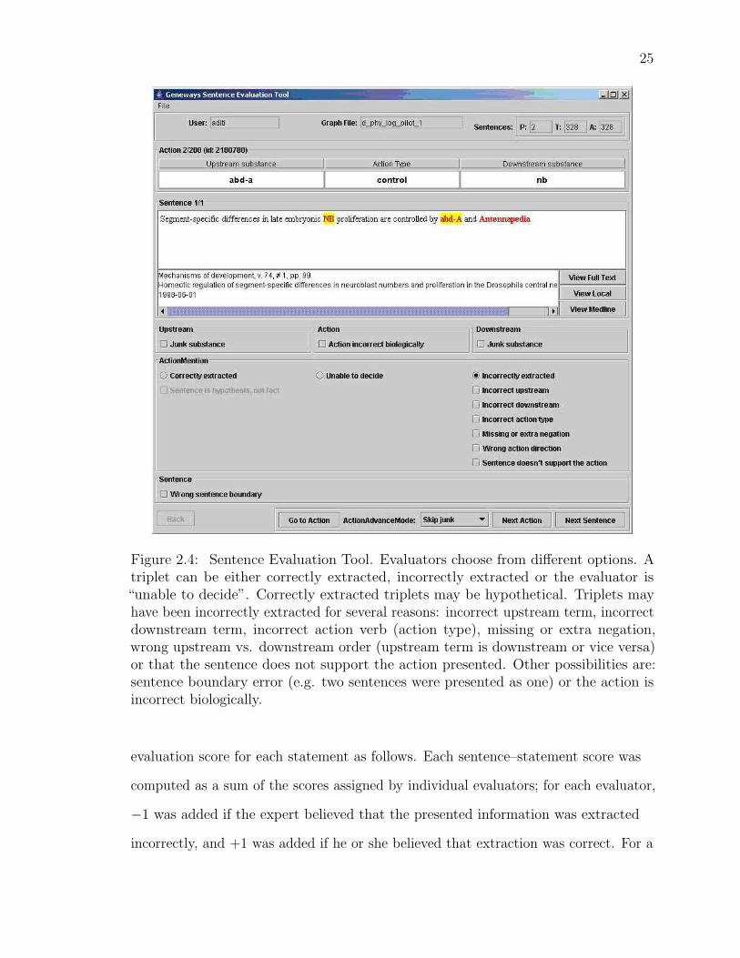
To facilitate evaluation, we developed a Sentence Evaluation Tool implemented in
Java programming language by Mitzi Morris and Ivan Iossifov, Figure 2.4. This tool
presented to an evaluator a set of annotation choices regarding each extracted fact;
the choices are listed in Table 2.2. The tool also presented in a single window the fact
itself and the sentence it was derived from. In the case a broader context was
required for the judgment, the evaluator had a choice to retrieve the complete journal
article containing this sentence by clicking a single button on the program interface.
For convenience of representing the results of manual evaluation, we computed an
2We also computed the κ-score for the inter-annotator agreement in the following way.
κ =P (A)− P (E)
1− P (E), (2.1)
where P (A) = 0.92 is the observed pair-wise agreement between annotators, P (E) is the expectedagreement under the random model (so long as we have a binary classification task, we assumedP (E) = 1
2 ), which gives κ = 0.84 for the high-agreement chunks and κ = 0.48 for the low-agreementchunk, see [75] for guidelines on usage and interpretation of κ-values. If we use a more sophisticatedrandom model, accounting for the observation that in our study an average evaluator assignedthe label correct with probability 0.65 rather than 0.5, we obtain P (E) = 0.652 + 0.352 = 0.545,which leads to slightly lower κ-estimates of 0.82 and 0.43, for the high- and low-agreement chunks,respectively.
3The low-agreement chunk was produced by only two evaluators. We interpreted the low agreementas an indication that the evaluators, while working on this chunk, were less careful than usual, andtreated this data set it in the same way as an experimentalist would treat a batch of potentiallycompromised experiments or expired reagents.
25
Figure 2.4: Sentence Evaluation Tool. Evaluators choose from different options. Atriplet can be either correctly extracted, incorrectly extracted or the evaluator is“unable to decide”. Correctly extracted triplets may be hypothetical. Triplets mayhave been incorrectly extracted for several reasons: incorrect upstream term, incorrectdownstream term, incorrect action verb (action type), missing or extra negation,wrong upstream vs. downstream order (upstream term is downstream or vice versa)or that the sentence does not support the action presented. Other possibilities are:sentence boundary error (e.g. two sentences were presented as one) or the action isincorrect biologically.
evaluation score for each statement as follows. Each sentence–statement score was
computed as a sum of the scores assigned by individual evaluators; for each evaluator,
−1 was added if the expert believed that the presented information was extracted
incorrectly, and +1 was added if he or she believed that extraction was correct. For a
26
set of three experts, this method permitted four possible scores: 3(1, 1, 1), 1(1, 1,−1),
−1(1,−1,−1), and −3. Similarly, for just two experts, the possible scores are 2(1, 1),
0(1,−1), and −2(−1,−1).4
2.4 Mathematical background
2.4.1 Machine-learning algorithms
General framework
The objects that we want to classify, the fact–sentence pairs, have complex properties.
We want to place each of them into one of two classes, correct or incorrect. In the
training data, each extracted fact is matched to a unique sentence from which it was
extracted, even though multiple sentences can express the same fact and a single
sentence can contain multiple facts. The ith object (the ith fact–sentence pair) comes
with a set of known features or properties that we encode into a feature vector, Fi:
Fi = (fi,1, fi,2, . . . , fi,n). (2.2)
In the following description we use C to indicate the random variable that represents
class (with possible values ccorrect and cincorrect), and F to represent a 1× n random
vector of feature values (also often called attributes), such that Fj is the jth element
of F . For example, for fact p53 activates JAK, feature F1 would have value 1 because
the upstream term p53 is found in a dictionary derived from the GenBank database
[85]; otherwise, it would have value 0.
4The actual scoring is slightly more complicated because a small portion of annotations providedby experts belonged to the class uncertain (corresponding to the option for evaluators “Unable todecide”), which was viewed as an intermediate between classes correct and incorrect—such annotationreceived a score of 0.

27
Sentence [Source] Extracted relation Evaluation(Confi-dence)
NIK binds to Nck in cultured cells. [76] nik bind nck Correct(High)
One is that presenilin is required for the propertrafficking of Notch and APP to their proteases,which may reside in an intracellular compart-ment. [77]
presenilin required for notch Correct(High)
Serine 732 phosphorylation of FAK by Cdk5 isimportant for microtubule organization, nuclearmovement, and neuronal migration. [78]
cdk5 phosphorylate fak Correct(High)
Histogram quantifying the percent of Arr2bound to rhodopsin-containing membranes af-ter treatment with blue light (B) or blue lightfollowed by orange light (BO). [79]
arr2 bind rhodopsin Correct(Low)
It is now generally accepted that a shift frommonomer to dimer and cadherin clustering ac-tivates classic cadherins at the surface into anadhesively competent conformation. [80]
cadherin activate cadherins Correct(Low)
Binding of G to CSP was four times greaterthan binding to syntaxin. [81]
csp bind syntaxin Incorrect(Low)
Treatment with NEM applied with cGMP madeactivation by cAMP more favorable by about2.5 kcal/mol. [82]
camp activate cgmp Incorrect(Low)
This matrix is likely to consist of actin filaments,as similar filaments can be induced by actin-stabilizing toxins (O. S. et al., unpublished data).[83]
actin induce actin Incorrect(High)
A ligand-gated association between cytoplas-mic domains of UNC5 and DCC family re-ceptors converts netrin-induced growth cone at-traction to repulsion. [84]
cytoplasmic domains asso-ciate unc5
Incorrect(High)
Table 2.1: Sentence examples.A sample of sentences that were used as an input to automated information extraction(the first column), biological relations extracted from these sentences (either correctlyor incorrectly, the second column), and the corresponding evaluations provided by 3human experts (the third column). A high-confidence label corresponds to a perfectagreement among all experts; a low-confidence label indicates that one of the expertsdisagreed with the other two.

28
Term levelUpstream term is a junk substanceAction is incorrect biologicallyDownstream term is a junk substance
Relation levelCorrectly extracted
Sentence is hypothesis, not factUnable to decideIncorrectly extracted
Incorrect upstreamIncorrect downstreamIncorrect action typeMissing or extra negationWrong action directionSentence does not support the action
Sentence levelWrong sentence boundary
Table 2.2: List of annotation choices available to the evaluators. The term “action”refers to the type of the extracted relation. For example, in statement A binds B“binds” is the action, “A” is the upstream term, and “B” is the downstream term.Action direction is defined as upstream to downstream, and “junk substance” is anobviously incorrectly identified term/entity.
Full Bayesian inference
The full Bayesian classifier assigns the ith object to the kth class if the posterior
probability P (C = ck|F = Fi) is greater for the kth class than for any alternative
class. This posterior probability is computed in the following way (a re-stated version
of Bayes’ theorem).
P (C = ck|F = Fi) = P (C = ck)×P (F = Fi|C = ck)
P (F = Fi). (2.3)
In the real-life applications, we estimate probability P (F = Fi|C = ck) from the
training data as a ratio of the number of objects that belong to the class ck and have
the same set of feature values as specified by the vector Fi to the total number of

29
objects in class ck in the training data.
In other words, we estimate the conditional probability for every possible value of the
feature vector F for every value of class C. Assuming that all features can be
discretized, we have to estimate
(v1 × v2 × . . . vn − 1)×m (2.4)
parameters, where vi is the number of discrete values observed for the ith feature and
m is the number of classes.
Clearly, even for a space of only 20 binary features5 the number of parameters that
we would need to estimate is (220 − 1)× 2 = 2, 097, 150, which exceeds several times
the number of data points in our training set.
Naıve Bayes classifier
The most affordable approximation to the full Bayesian analysis is the Naıve Bayes
classifier. It is based on the assumption of conditional independence of features:
P (F = Fi|C = ck) = P (F1 = fi,1|C = ck)
× P (F2 = fi,2|C = ck) . . .
× P (Fn = fi,n|C = ck) . (2.5)
Obviously, we can estimate P (Fj = fi,j|C = ck)’s reasonably well with a relatively
small set of training data, but the assumption of conditional independence (Equation
2.5) comes at a price: the Naıve Bayes classifier is usually markedly less successful in
its job than are its more sophisticated relatives.6
5We used 68 features, most of which are non-binary, see Table 2.5.6The only exception occurs when the features are truly conditionally independent of one another.
In this special case both methods should have an identical performance. The same reasoning applies
30
In an application with m classes and n features (given that the ith feature has vi
admissible discrete values), a Naıve Bayes algorithm requires estimation of
m×∑
i=1,n(vi − 1) parameters (which value, in our case, is equal to 4, 208).
Middle ground between the full and Naıve Bayes: Clustered Bayes
We can find an intermediate ground between the full and Naıve Bayes classifiers by
assuming that features in the random vector F are arranged into groups or clusters,
such that all features within the same cluster are dependent on one another
(conditionally on the class), and all features from different classes are conditionally
independent. That is, we can assume that the feature random vector (F) and the
observed feature vector for the ith object (Fi) can be partitioned into sub-vectors:
F = (Φ1,Φ2, . . . ,ΦM), and (2.6)
Fi = (fi,1, fi,2, . . . , fi,M), (2.7)
respectively, where Φj is the jth cluster of features; fi,j is the set of values for this
cluster with respect to the ith object, and M is the total number of clusters of
features.
The Clustered Bayes classifier is based on the following assumption about conditional
independence of clusters of features:
to all other approximations of the full Bayesian analysis (Clustered Bayes, Discriminant Analysis, andMaximum Entropy methods): They should perform less accurately than the full Bayesian analysiswhenever their assumptions are not matched exactly by the data, and perform identically to the fullBayesian analysis otherwise.
31
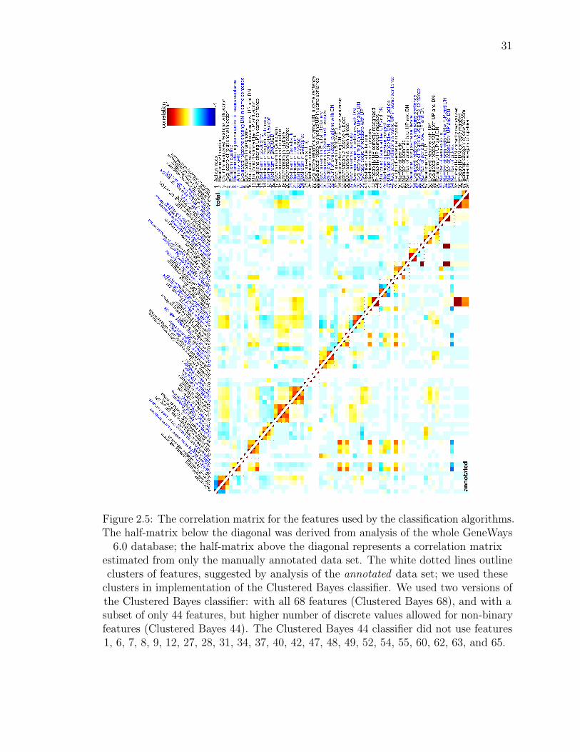
Figure 2.5: The correlation matrix for the features used by the classification algorithms.The half-matrix below the diagonal was derived from analysis of the whole GeneWays
6.0 database; the half-matrix above the diagonal represents a correlation matrixestimated from only the manually annotated data set. The white dotted lines outlineclusters of features, suggested by analysis of the annotated data set; we used these
clusters in implementation of the Clustered Bayes classifier. We used two versions ofthe Clustered Bayes classifier: with all 68 features (Clustered Bayes 68), and with asubset of only 44 features, but higher number of discrete values allowed for non-binaryfeatures (Clustered Bayes 44). The Clustered Bayes 44 classifier did not use features1, 6, 7, 8, 9, 12, 27, 28, 31, 34, 37, 40, 42, 47, 48, 49, 52, 54, 55, 60, 62, 63, and 65.

32
P (F = Fi|C = ck) = P (Φ1 = fi,1|C = ck)
× P (Φ2 = fi,2|C = ck) . . .
× P (ΦM = fi,M |C = ck) . (2.8)
We tested two versions of the Clustered Bayes classifier: one version used all 68
features (Clustered Bayes 68) with a coarser discretization of feature values; another
version used a subset of 44 features (Clustered Bayes 44) but allowed for more
discrete values for each continuous-valued feature, see legend to Figure 2.5.
Linear and quadratic discriminants
Another method that can be viewed as an approximation to full Bayesian analysis is
Discriminant Analysis invented by Sir Ronald A. Fisher [86]. This method requires
no assumption about conditional independence of features; instead, it assumes that
the conditional probability P (F = Fi|C = ck) is a multivariate normal distribution.
P (F = Fi|C = ck) =e−
12(Fi−µk)′V−1
k (Fi−µk)√(2π)n |Vk|
, (2.9)
where n is the total number of features/variables in the class-specific multivariate
distributions. The method has two variations. The first, Linear Discriminant
Analysis, assumes that different classes have different mean values for features
(vectors µk), but the same variance-covariance matrix, V = Vk for all k.7 In the
second variation, Quadratic Discriminant Analysis (QDA), the assumption of the
common variance-covariance matrix for all classes, is relaxed, such that every class is
assumed to have a distinct variance-covariance matrix, Vk.8
7These assumptions lead to a linear optimal decision boundary, as reflected by the name of themethod.
8This change in assumptions leads to a quadratic optimal decision boundary.
33
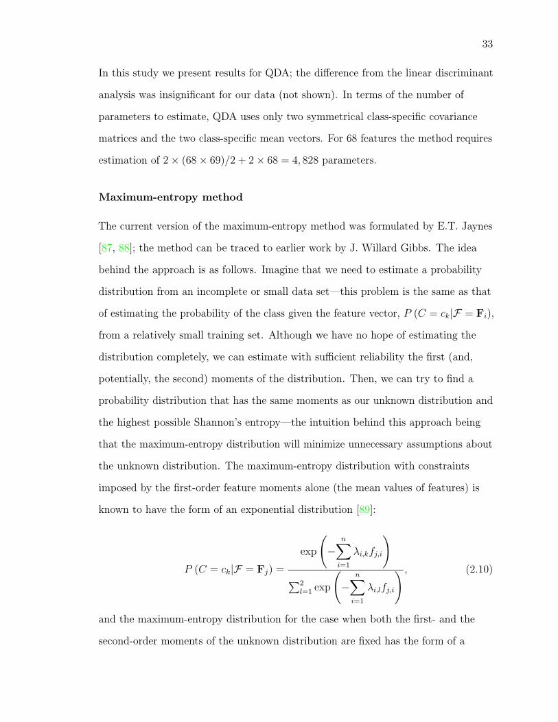
In this study we present results for QDA; the difference from the linear discriminant
analysis was insignificant for our data (not shown). In terms of the number of
parameters to estimate, QDA uses only two symmetrical class-specific covariance
matrices and the two class-specific mean vectors. For 68 features the method requires
estimation of 2× (68× 69)/2 + 2× 68 = 4, 828 parameters.
Maximum-entropy method
The current version of the maximum-entropy method was formulated by E.T. Jaynes
[87, 88]; the method can be traced to earlier work by J. Willard Gibbs. The idea
behind the approach is as follows. Imagine that we need to estimate a probability
distribution from an incomplete or small data set—this problem is the same as that
of estimating the probability of the class given the feature vector, P (C = ck|F = Fi),
from a relatively small training set. Although we have no hope of estimating the
distribution completely, we can estimate with sufficient reliability the first (and,
potentially, the second) moments of the distribution. Then, we can try to find a
probability distribution that has the same moments as our unknown distribution and
the highest possible Shannon’s entropy—the intuition behind this approach being
that the maximum-entropy distribution will minimize unnecessary assumptions about
the unknown distribution. The maximum-entropy distribution with constraints
imposed by the first-order feature moments alone (the mean values of features) is
known to have the form of an exponential distribution [89]:
P (C = ck|F = Fj) =
exp
(−
n∑i=1
λi,kfj,i
)∑2
l=1 exp
(−
n∑i=1
λi,lfj,i
) , (2.10)
and the maximum-entropy distribution for the case when both the first- and the
second-order moments of the unknown distribution are fixed has the form of a

34
multidimensional normal distribution [89]. The conditional distribution that we are
trying to estimate can be written in the following exponential form:
P (C = ck|F = Fj) =
exp
(−
n∑i=1
λi,kfj,i −n∑x=1
n∑y=x
νx,y,kfj,xfj,y
)∑2
l=1 exp
(−
n∑i=1
λi,lfj,i −n∑x=1
n∑y=x
νx,y,lfj,xfj,y
) . (2.11)
Parameters λi,k’s and νx,y,k’s are k-class-specific weights of individual features and
feature pairs, respectively, and in principle can be expressed in terms of the first and
second moments of the distributions. The values of parameters in Equations 2.10 and
2.11 are estimated by maximizing the product of probabilities for the individual
training examples.
We tested two versions of the maximum-entropy classifier. MaxEnt 1 uses only
information about the first moments of features in the training data (Equation 2.10);
MaxEnt 2 uses the set of all individual features and the products of feature pairs
(Equation 2.11). To select the most informative pairs of features we used a mutual
information approach, as described in the subsection dealing with classification
features.
For two classes (correct and incorrect) and 68 features MaxEnt 1 requires estimation
of 136 parameters. In contrast, MaxEnt 2 requires estimation of 4, 828 parameters:
weight parameters for all first moments for two classes, plus weights for the second
moments for two classes. MaxEnt 2-v is a version of MaxEnt 2 classifier where the
squared values of features are not used, so that the classifier requires estimation of
only 4, 692 weight parameters.

35
Figure 2.6: A hypothetical three-layered feed-forward neural network. We useda similar network with 68 input units (one unit per classification feature) and 10hidden-layer units.
Feed-forward neural network
A typical feed-forward artificial neural network is a directed acyclic graph organized
into three (or more) layers. In our case, we chose a three-layered network, with a set
of nodes of the input layer, {xi}i=1,...,Nx , nodes of the hidden layer, {yj}j=1,...,Ny , and
a single node representing the output layer, z1, see Figure 2.6. The number of input
nodes, Nx, is determined by the number of features used in the analysis (68 in our
case). The number of hidden nodes, Ny, determines both the network’s expressive
power and its ability to generalize. Too small a number of hidden nodes makes a
simplistic network that cannot learn from complex data. Too large a number makes a
network that tends to overtrain—that works perfectly on the training data, but poorly
on new data. We experimented with different values of Ny and settled on Ny = 10.
The values of the input nodes, {xi}i=1,...,Nx , are feature values of the object that we
need to classify. The value of each node, yj, in the hidden layer is determined in the
following way:
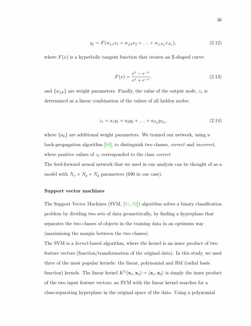
36
yj = F (wj,1x1 + wj,2x2 + . . .+ wj,NxxNx), (2.12)
where F (x) is a hyperbolic tangent function that creates an S-shaped curve:
F (x) =ex − e−x
ex + e−x, (2.13)
and {wj,k} are weight parameters. Finally, the value of the output node, z1 is
determined as a linear combination of the values of all hidden nodes:
z1 = a1y1 + a2y2 + . . .+ aNyyNy , (2.14)
where {ak} are additional weight parameters. We trained our network, using a
back-propagation algorithm [90], to distinguish two classes, correct and incorrect,
where positive values of z1 corresponded to the class correct.
The feed-forward neural network that we used in our analysis can be thought of as a
model with Nx ×Ny +Ny parameters (690 in our case).
Support vector machines
The Support Vector Machines (SVM, [91, 92]) algorithm solves a binary classification
problem by dividing two sets of data geometrically, by finding a hyperplane that
separates the two classes of objects in the training data in an optimum way
(maximizing the margin between the two classes).
The SVM is a kernel -based algorithm, where the kernel is an inner product of two
feature vectors (function/transformation of the original data). In this study, we used
three of the most popular kernels: the linear, polynomial and Rbf (radial basis
function) kernels. The linear kernel KL(x1,x2) = 〈x1,x2〉 is simply the inner product
of the two input feature vectors; an SVM with the linear kernel searches for a
class-separating hyperplane in the original space of the data. Using a polynomial

37
kernel, KPd (x1,x2) = (1 + 〈x1,x2〉)d, is equivalent to transforming the data into a
higher-dimensional space and searching for a separating plane there.9 Finally, using
an Rbf kernel, KRbfg (x1,x2) = e−g‖x1−x2‖2 , corresponds to finding a separating
hyperplane in an infinite-dimensional space.
In the most real-world cases the two classes cannot be separated perfectly by a
hyperplane, and some classification errors are unavoidable. SVM algorithms use the
C-parameter to control the error rate during the training phase (if the error is not
constrained, the margin of every hyperplane can be extended infinitely). In this study,
we used the default values for the C-parameter suggested by the SVM Light tool.
Table 2.3 lists the SVM models and C-parameter values that we used in this study.
Model Kernel Kernel parameter C-parameterSVM (OSU SVM) Linear 1SVM-t0 (SVM Light) Linear 1SVM-t1-d2 Polynomial d = 2 0.3333SVM-t1-d3 Polynomial d = 3 0.1429SVM-t2-g0.5 Rbf g = 0.5 1.2707SVM-t2-g1 Rbf g = 1 0.7910SVM-t2-g2 Rbf g = 2 0.5783
Table 2.3: Parameter values used for various SVM classifiers in this study.
The output of an SVM analysis is not probabilistic, but there are tools to convert an
SVM classification output into “posterior probabilities,” see chapter by J. Platt in
[93]. (A similar comment is applicable to the artificial neural network.)
The number of support vectors used by the SVM classifier depends on the size and
properties of the training data set. The average number of (1× 68-dimensional)
support vectors used in 10 cross-validation experiments was 12, 757.5, 11, 994.4,
12, 092, 12, 289.9, 12, 679.7, and 14, 163.8, for SVM, SVM-t1-d2, SVM-t1-d3,
SVM-t2-g0.5, SVM-t2-g1, and SVM-t2-g2 classifiers, respectively. The total number
of data-derived values (which we loosely call “parameters”) used by the SVM in our
9For example, if the original space is two-dimensional x = (x1, x2) and the degree d of thepolynomial kernel is 2, the implicit transformation is h(x) = (1,
√2x1,
√2x2, x
21, x
22,√
2x1x2).
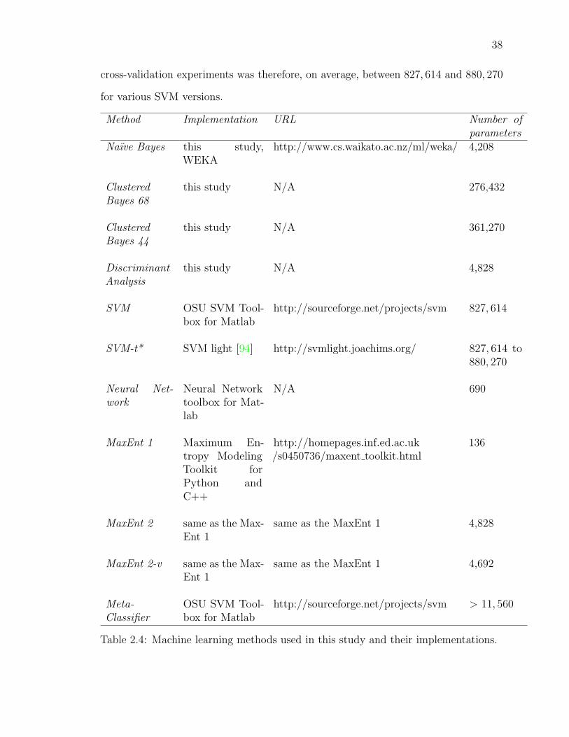
38
cross-validation experiments was therefore, on average, between 827, 614 and 880, 270
for various SVM versions.
Method Implementation URL Number ofparameters
Naıve Bayes this study,WEKA
http://www.cs.waikato.ac.nz/ml/weka/ 4,208
ClusteredBayes 68
this study N/A 276,432
ClusteredBayes 44
this study N/A 361,270
DiscriminantAnalysis
this study N/A 4,828
SVM OSU SVM Tool-box for Matlab
http://sourceforge.net/projects/svm 827, 614
SVM-t* SVM light [94] http://svmlight.joachims.org/ 827, 614 to880, 270
Neural Net-work
Neural Networktoolbox for Mat-lab
N/A 690
MaxEnt 1 Maximum En-tropy ModelingToolkit forPython andC++
http://homepages.inf.ed.ac.uk/s0450736/maxent toolkit.html
136
MaxEnt 2 same as the Max-Ent 1
same as the MaxEnt 1 4,828
MaxEnt 2-v same as the Max-Ent 1
same as the MaxEnt 1 4,692
Meta-Classifier
OSU SVM Tool-box for Matlab
http://sourceforge.net/projects/svm > 11, 560
Table 2.4: Machine learning methods used in this study and their implementations.

39
Meta-method
We implemented the meta-classifier on the basis of the SVM algorithm (linear kernel
with C = 1) applied to predictions (converted into probabilities that the object
belongs to the class correct) provided by the individual “simple” classifiers. The
meta-method used 1, 445 support vectors (1× 7-dimensional), in addition to combined
parameters of the seven individual classifiers used as input to the meta-classifier.
Implementation
A summary of the sources of software used in our study is shown in Table 2.4.
2.4.2 Features used in our analysis
We selected 68 individual features covering a range of characteristics that could help
in the classification, see Table 2.5. To capture the flow of information in a molecular
interaction graph (the edge direction), in each extracted relation we identified an
“upstream term” (corresponding to the graph node with the outgoing directed edge)
and a “downstream term” (the node with the incoming directed edge): for example,
in the phrase “JAK phosphorylates p53,” JAK is the upstream term, and p53 is the
downstream term. Features in the group keywords represent a list of tokens that may
signal that the sentence is hypothetical, interrogative, negative, or that there is a
confusion in the relation extraction (e.g. the particle “by” in passive-voice sentences).
We eventually abandoned keywords as we found them to be uninformative features,
but they are still listed for the sake of completeness.
To represent the second-order features (pairs of features), we defined a new feature as
a product of the normalized values of two features. We obtained the normalized
values of features by subtracting the mean value from each feature value, then
dividing the result by the standard deviation for this feature.
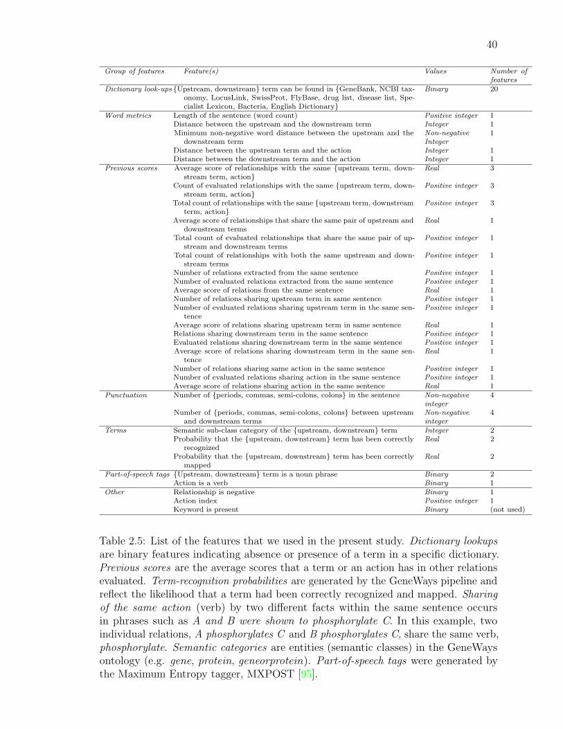
40
Group of features Feature(s) Values Number offeatures
Dictionary look-ups {Upstream, downstream} term can be found in {GeneBank, NCBI tax-onomy, LocusLink, SwissProt, FlyBase, drug list, disease list, Spe-cialist Lexicon, Bacteria, English Dictionary}
Binary 20
Word metrics Length of the sentence (word count) Positive integer 1Distance between the upstream and the downstream term Integer 1Minimum non-negative word distance between the upstream and the
downstream termNon-negativeInteger
1
Distance between the upstream term and the action Integer 1Distance between the downstream term and the action Integer 1
Previous scores Average score of relationships with the same {upstream term, down-stream term, action}
Real 3
Count of evaluated relationships with the same {upstream term, down-stream term, action}
Positive integer 3
Total count of relationships with the same {upstream term, downstreamterm, action}
Positive integer 3
Average score of relationships that share the same pair of upstream anddownstream terms
Real 1
Total count of evaluated relationships that share the same pair of up-stream and downstream terms
Positive integer 1
Total count of relationships with both the same upstream and down-stream terms
Positive integer 1
Number of relations extracted from the same sentence Positive integer 1Number of evaluated relations extracted from the same sentence Positive integer 1Average score of relations from the same sentence Real 1Number of relations sharing upstream term in same sentence Positive integer 1Number of evaluated relations sharing upstream term in the same sen-
tencePositive integer 1
Average score of relations sharing upstream term in same sentence Real 1Relations sharing downstream term in the same sentence Positive integer 1Evaluated relations sharing downstream term in the same sentence Positive integer 1Average score of relations sharing downstream term in the same sen-
tenceReal 1
Number of relations sharing same action in the same sentence Positive integer 1Number of evaluated relations sharing action in the same sentence Positive integer 1Average score of relations sharing action in the same sentence Real 1
Punctuation Number of {periods, commas, semi-colons, colons} in the sentence Non-negativeinteger
4
Number of {periods, commas, semi-colons, colons} between upstreamand downstream terms
Non-negativeinteger
4
Terms Semantic sub-class category of the {upstream, downstream} term Integer 2Probability that the {upstream, downstream} term has been correctly
recognizedReal 2
Probability that the {upstream, downstream} term has been correctlymapped
Real 2
Part-of-speech tags {Upstream, downstream} term is a noun phrase Binary 2Action is a verb Binary 1
Other Relationship is negative Binary 1Action index Positive integer 1Keyword is present Binary (not used)
Table 2.5: List of the features that we used in the present study. Dictionary lookupsare binary features indicating absence or presence of a term in a specific dictionary.Previous scores are the average scores that a term or an action has in other relationsevaluated. Term-recognition probabilities are generated by the GeneWays pipeline andreflect the likelihood that a term had been correctly recognized and mapped. Sharingof the same action (verb) by two different facts within the same sentence occursin phrases such as A and B were shown to phosphorylate C. In this example, twoindividual relations, A phosphorylates C and B phosphorylates C, share the same verb,phosphorylate. Semantic categories are entities (semantic classes) in the GeneWaysontology (e.g. gene, protein, geneorprotein). Part-of-speech tags were generated bythe Maximum Entropy tagger, MXPOST [95].

41
2.4.3 Separating data into training and testing:
Cross-validation
To evaluate the success of our classifiers we used a 10-fold cross-validation approach,
where we used 910
of data for training and 110
for testing. More precisely, given a
partition of the manually evaluated data into 10 equal portions, we created 10
different pairs of training-test subsets, where we used each of the 10 equal data
subsets in turn as testing data set, and used the larger remaining data subset as the
training set. We then used 10 training-test set pairs to compare all algorithms.
2.4.4 Comparison of methods: Receiver operating
characteristic (ROC) scores
To quantify and compare success of the various classification methods we used receiver
operating characteristic (ROC) scores, also called areas under ROC curve [96].
An ROC score is computed in the following way. All test-set predictions of a
particular classification method are ordered by the decreasing quality score provided
by this method; for example, in the case of the Clustered Bayes algorithm, the quality
score is the posterior probability that the test object belongs to the class correct. The
ranked list is then converted into binary predictions by applying a decision threshold,
T : All test objects with a quality score above T are classified as correct and all test
objects with low-than-threshold scores are classified as incorrect. The ROC score is
then computed by plotting the proportion of true-positive predictions (in the test set
we know both the correct label and the quality score of each object) against
false-positive predictions for the whole spectrum of possible values of T , then
integrating the area under the curve obtained in this way, see Figure 2.7.
The ROC score is an estimate of the probability that the classifier under scrutiny will
label correctly a pair of statements, one of which is from the class correct and one
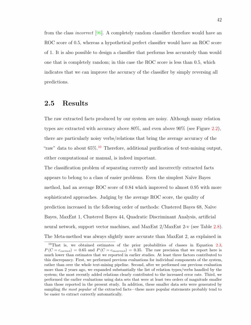
42
from the class incorrect [96]. A completely random classifier therefore would have an
ROC score of 0.5, whereas a hypothetical perfect classifier would have an ROC score
of 1. It is also possible to design a classifier that performs less accurately than would
one that is completely random; in this case the ROC score is less than 0.5, which
indicates that we can improve the accuracy of the classifier by simply reversing all
predictions.
2.5 Results
The raw extracted facts produced by our system are noisy. Although many relation
types are extracted with accuracy above 80%, and even above 90% (see Figure 2.2),
there are particularly noisy verbs/relations that bring the average accuracy of the
“raw” data to about 65%.10 Therefore, additional purification of text-mining output,
either computational or manual, is indeed important.
The classification problem of separating correctly and incorrectly extracted facts
appears to belong to a class of easier problems. Even the simplest Naıve Bayes
method, had an average ROC score of 0.84 which improved to almost 0.95 with more
sophisticated approaches. Judging by the average ROC score, the quality of
prediction increased in the following order of methods: Clustered Bayes 68, Naıve
Bayes, MaxEnt 1, Clustered Bayes 44, Quadratic Discriminant Analysis, artificial
neural network, support vector machines, and MaxEnt 2/MaxEnt 2-v (see Table 2.8).
The Meta-method was always slightly more accurate than MaxEnt 2, as explained in
10That is, we obtained estimates of the prior probabilities of classes in Equation 2.3,P (C = ccorrect) = 0.65 and P (C = cincorrect) = 0.35. The raw precision that we report here ismuch lower than estimates that we reported in earlier studies. At least three factors contributed tothis discrepancy. First, we performed previous evaluations for individual components of the system,rather than over the whole text-mining pipeline. Second, after we performed our previous evaluationmore than 2 years ago, we expanded substantially the list of relation types/verbs handled by thesystem; the most recently added relations clearly contributed to the increased error rate. Third, weperformed the earlier evaluations using data sets that were at least two orders of magnitude smallerthan those reported in the present study. In addition, these smaller data sets were generated bysampling the most popular of the extracted facts—these more popular statements probably tend tobe easier to extract correctly automatically.

43
legend to Table 2.8 and shown in Figure 2.7.
Table 2.8 provides a somewhat misleading impression that MaxEnt 2 and MaxEnt 2-v
are not significantly more accurate than their closest competitors (the SVM family),
because of the overlapping confidence intervals. However, when we trace the
performance of all classifiers in individual cross-validation experiments (see Figure
2.9) it becomes clear that MaxEnt 2 and MaxEnt 2-v outperformed their rivals in
every cross-validation experiment. The SVM and artificial neural network methods
performed essentially identically, and were always more accurate than three other
methods: QDA, Clustered Bayes 44, and MaxEnt 1. Finally, the performance of the
Clustered Bayes 68 and the Naıve Bayes methods was reliably the least accurate of all
methods studied.
It is a matter of both academic curiosity and of practical importance to know how the
performance of our artificial intelligence curator compares to that of humans. If we
define the correct answer as a majority-vote of the three human evaluators (see Table
2.6), the average accuracy of MaxEnt 2 is slightly lower than, but statistically
indistinguishable from humans (at the 99% level of significance, see Table 2.6; capital
letters “A”, “L”, “S”, and “M” hide the real names of the human evaluators). If,
however, in the spirit of Turing’s test of machine intelligence [97], we treat the
MaxEnt 2 algorithm on an equal footing with the human evaluators, compute the
average over predictions of all four anonymous evaluators, and compare the quality of
the performance of each evaluator with regard to the average, MaxEnt 2 always
performs slightly more accurately than one of the human evaluators.11 (In all cases
we compared performance of the algorithm on data that was not used for its training;
11Alan M. Turing proposed an experiment for testing machine intelligence by interrogating themachine and a group of humans through a mediator, the goal being to distinguish the humans fromthe machine on the basis of only typewritten replies. If the interrogator fails to make the correctdistinction, machine intelligence passes the test. Applying the Turing test to our problem, we imaginethat we have a group of four evaluators, one of which is a computer. If we cannot single out thecomputer-embodied evaluator on the basis of a higher error rate, our artificial evaluator passes thetest.
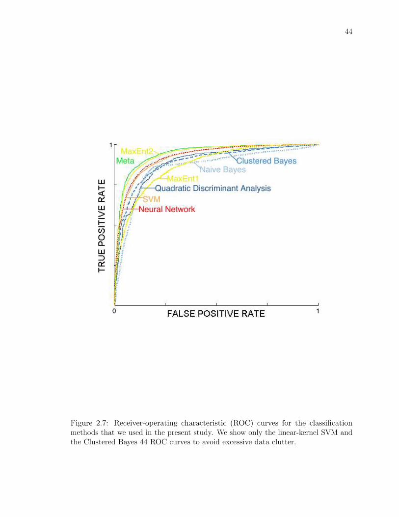
44
Figure 2.7: Receiver-operating characteristic (ROC) curves for the classificationmethods that we used in the present study. We show only the linear-kernel SVM andthe Clustered Bayes 44 ROC curves to avoid excessive data clutter.
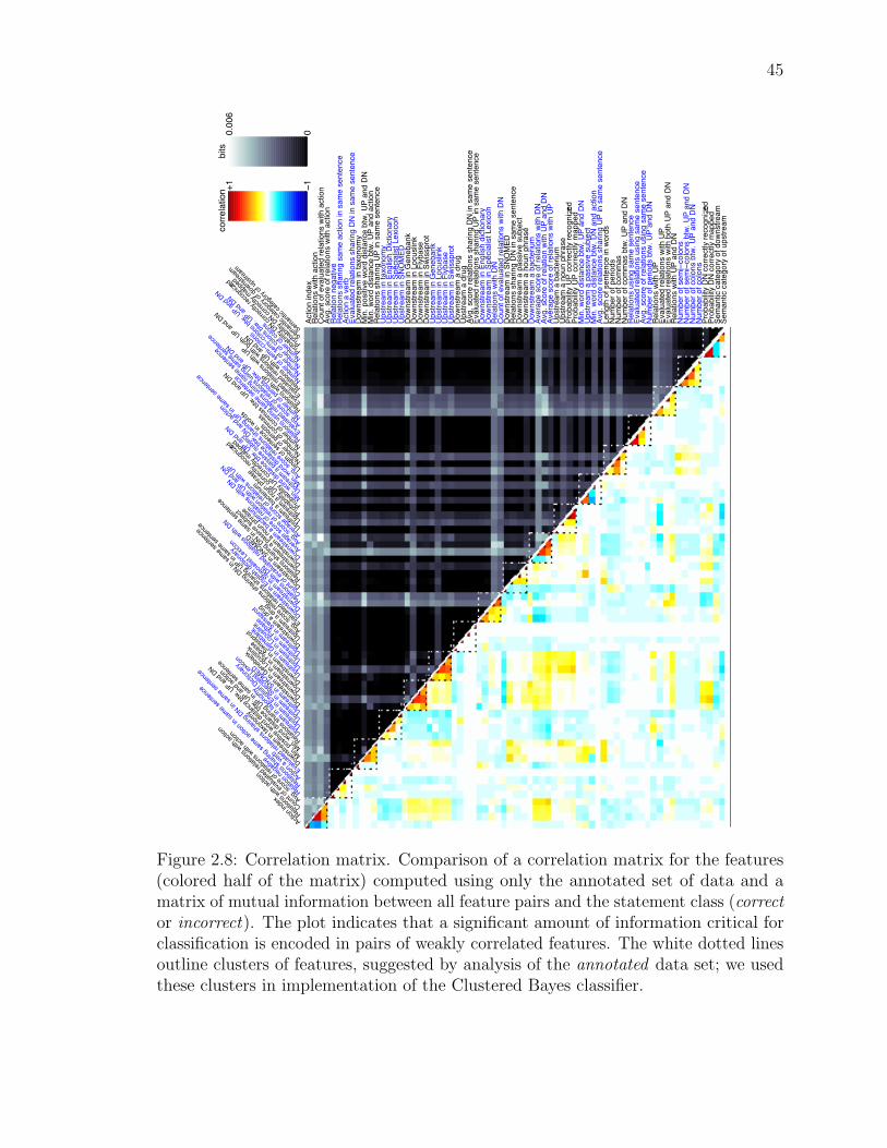
45
00.0
06
Action index
Actio
n in
dex
Rela
tions w
ith a
ction
Rel
atio
ns w
ith a
ctio
n
Count
of
evalu
ate
d r
ela
tions w
ith a
ction
Cou
nt o
f eva
luat
ed re
latio
ns w
ith a
ctio
n
Avg.
score
of
rela
tions w
ith a
ction
Avg. s
core
of r
elat
ions
with
act
ion
Rela
tion n
egative
Rel
atio
n ne
gativ
e
Rela
tions s
haring s
am
e a
ction in s
am
e s
ente
nce
Rel
atio
ns s
harin
g sa
me
actio
n in
sam
e se
nten
ce
Action a
verb
Actio
n a
verb
Evalu
ate
d r
ela
tions s
haring D
N in s
am
e s
ente
nce
Evalu
ated
rela
tions
sha
ring
DN
in s
ame
sent
ence
Dow
nstr
eam
in t
axonom
y
Dow
nstre
am in
taxo
nom
y
Min
. positiv
e w
ord
dis
tance b
tw.
UP
and D
N
Min
. pos
itive
wor
d di
stan
ce b
tw. U
P and
DN
Min
. w
ord
dis
tance b
tw.
UP
and a
ction
Min
. wor
d di
stan
ce b
tw. U
P and
act
ion
Rela
tions s
haring U
P in s
am
e s
ente
nce
Rel
atio
ns s
harin
g U
P in s
ame
sent
ence
Upstr
eam
in t
axonom
y
Ups
tream
in ta
xono
my
Upstr
eam
in E
nglis
h D
ictionary
Ups
tream
in E
nglis
h D
ictio
nary
Upstr
eam
in S
pecia
list
Lexic
on
Ups
tream
in S
peci
alis
t Lex
icon
Upstr
eam
in S
NO
ME
D
Ups
tream
in S
NO
MED
Dow
nstr
eam
in G
enebank
Dow
nstre
am in
Gen
eban
k
Dow
nstr
eam
in L
ocuslin
k
Dow
nstre
am in
Loc
uslin
k
Dow
nstr
eam
in F
lybase
Dow
nstre
am in
Fly
base
Dow
nstr
eam
in S
wis
spro
t
Dow
nstre
am in
Sw
issp
rot
Upstr
eam
in G
enebank
Ups
tream
in G
eneb
ank
Upstr
eam
in L
ocuslin
k
Ups
tream
in L
ocus
link
Upstr
eam
in F
lybase
Ups
tream
in F
lyba
se
Upstr
eam
in S
wis
spro
t
Ups
tream
in S
wis
spro
t
Dow
nstr
eam
a d
rug
Dow
nstre
am a
dru
g
Upstr
eam
a d
rug
Ups
tream
a d
rug
Avg.
score
rela
tions s
haring D
N in s
am
e s
ente
nce
Avg. s
core
rela
tions
sha
ring
DN
in s
ame
sent
ence
Evalu
ate
d r
ela
tions s
haring U
P in s
am
e s
ente
nce
Evalu
ated
rela
tions
sha
ring
UP in
sam
e se
nten
ce
Dow
nstr
eam
in E
nglis
h d
ictionary
Dow
nstre
am in
Eng
lish
dict
iona
ry
Dow
nstr
eam
in S
pecia
list
Lexic
on
Dow
nstre
am in
Spe
cial
ist L
exic
on
Rela
tions w
ith D
N
Rel
atio
ns w
ith D
N
Count
of
evalu
ate
d r
ela
tions w
ith D
N
Cou
nt o
f eva
luat
ed re
latio
ns w
ith D
N
Dow
nstr
eam
in S
NO
ME
D
Dow
nstre
am in
SN
OM
ED
Rela
tions s
haring D
N in s
am
e s
ente
nce
Rel
atio
ns s
harin
g D
N in
sam
e se
nten
ce
Dow
nstr
eam
a p
assiv
e s
ubje
ct
Dow
nstre
am a
pas
sive
sub
ject
!1
Dow
nstr
eam
a n
oun p
hra
se
Dow
nstre
am a
nou
n ph
rase
Dow
nstr
eam
a b
acte
rium
Dow
nstre
am a
bac
teriu
m
Avera
ge s
core
of
rela
tions w
ith D
N
Avera
ge s
core
of r
elat
ions
with
DN
Avg.
score
of
rela
tion w
ith U
P a
nd D
NAvg
. sco
re o
f rel
atio
n w
ith U
P and
DN
Avera
ge s
core
of
rela
tions w
ith U
P
Avera
ge s
core
of r
elat
ions
with
UP
Upstr
eam
a b
acte
rium
Ups
tream
a b
acte
rium
Upstr
eam
a n
oun p
hra
se
Ups
tream
a n
oun
phra
se
Pro
babili
ty U
P c
orr
ectly r
ecogniz
ed
Proba
bilit
y U
P cor
rect
ly re
cogn
ized
Pro
babili
ty U
P c
orr
ectly m
apped
Proba
bilit
y U
P cor
rect
ly m
appe
d
Min
. w
ord
dis
tance b
tw.
UP
and D
N
Min
. wor
d di
stan
ce b
tw. U
P and
DN
Upstr
eam
a p
assiv
e s
ubje
ct
Ups
tream
a p
assi
ve s
ubje
ct
Min
. w
ord
dis
tance b
tw.
DN
and a
ction
Min
. wor
d di
stan
ce b
tw. D
N a
nd a
ctio
n
Avg.
score
rela
tions s
haring U
P in s
am
e s
ente
nce
Avg. s
core
rela
tions
sha
ring
UP in
sam
e se
nten
ce
Length
of
sente
nce in w
ord
s
Leng
th o
f sen
tenc
e in
wor
ds
Num
ber
of
periods
Num
ber o
f per
iods
Num
ber
of
com
mas
Num
ber o
f com
mas
Num
ber
of
com
mas b
tw.
UP
and D
N
Num
ber o
f com
mas
btw
. UP a
nd D
N
Rela
tions u
sin
g s
am
e s
ente
nce
Rel
atio
ns u
sing
sam
e se
nten
ce
Evalu
ate
d r
ela
tions u
sin
g s
am
e s
ente
nce
Evalu
ated
rela
tions
usi
ng s
ame
sent
ence
Avg.
score
of
rela
tions u
sin
g s
am
e s
ente
nce
Avg. s
core
of r
elat
ions
usi
ng s
ame
sent
ence
Num
ber
of
periods b
tw.
UP
and D
N
Num
ber o
f per
iods
btw
. UP a
nd D
N
Rela
tions w
ith U
P
Rel
atio
ns w
ith U
P
Evalu
ate
d r
ela
tions w
ith U
P
Evalu
ated
rela
tions
with
UP
Evalu
ate
d r
ela
tions w
ith b
oth
UP
and D
N
Evalu
ated
rela
tions
with
bot
h U
P and
DN
Rela
tions w
ith U
P a
nd D
N
Rel
atio
ns w
ith U
P and
DN
Num
ber
of
sem
i!colo
ns
Num
ber o
f sem
i!co
lons
Num
ber
of
sem
i!colo
ns b
tw.
UP
and D
N
Num
ber o
f sem
i!co
lons
btw
. UP a
nd D
N
Num
ber
of
colo
ns b
tw.
UP
and D
N
Num
ber o
f col
ons
btw
. UP a
nd D
N
Num
ber
of
colo
ns
Num
ber o
f col
ons P
robabili
ty D
N c
orr
ectly r
ecogniz
ed
Proba
bilit
y D
N c
orre
ctly
reco
gniz
ed
Pro
babili
ty D
N c
orr
ectly m
apped
Proba
bilit
y D
N c
orre
ctly
map
ped
Sem
antic c
ate
gory
of
dow
nstr
eam
Seman
tic c
ateg
ory
of d
owns
tream
Sem
antic c
ate
gory
of
upstr
eam
bits
Seman
tic c
ateg
ory
of u
pstre
am
+1
corr
ela
tion
Figure 2.8: Correlation matrix. Comparison of a correlation matrix for the features(colored half of the matrix) computed using only the annotated set of data and amatrix of mutual information between all feature pairs and the statement class (corrector incorrect). The plot indicates that a significant amount of information critical forclassification is encoded in pairs of weakly correlated features. The white dotted linesoutline clusters of features, suggested by analysis of the annotated data set; we usedthese clusters in implementation of the Clustered Bayes classifier.
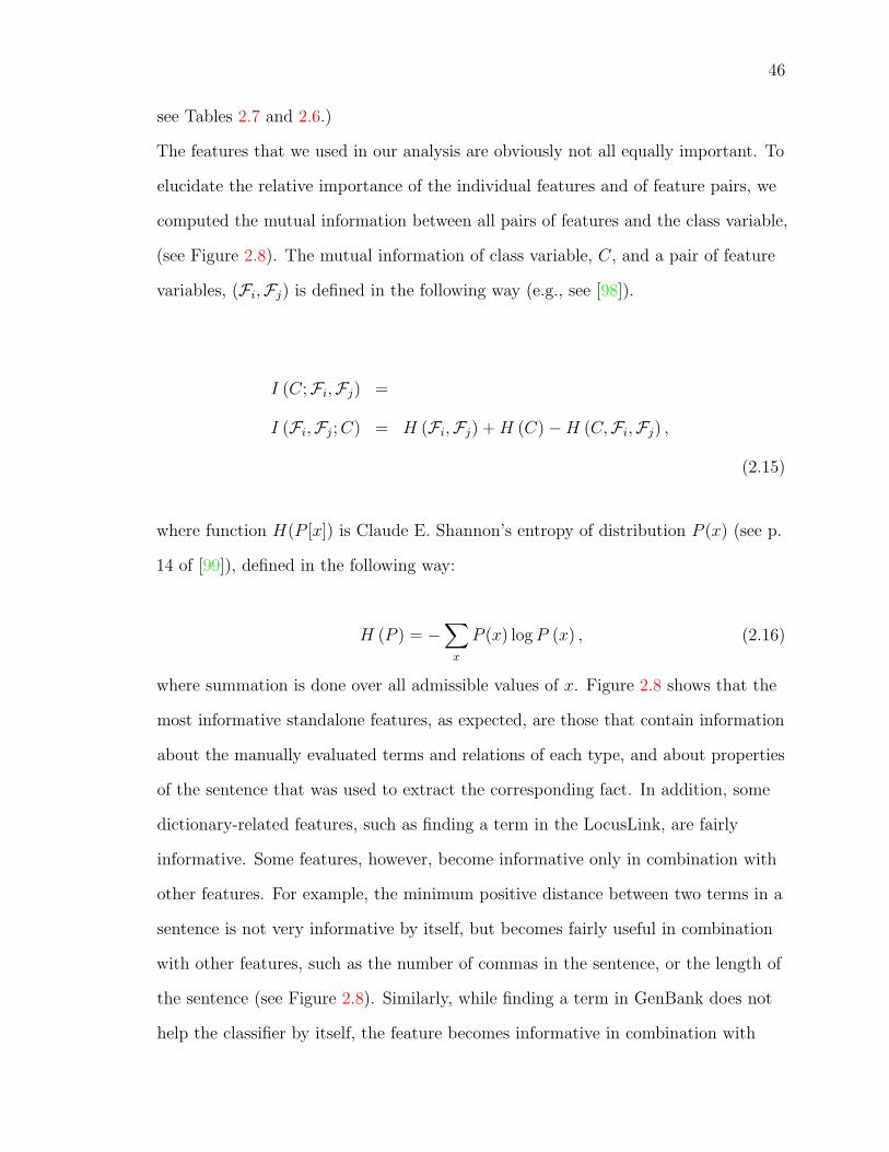
46
see Tables 2.7 and 2.6.)
The features that we used in our analysis are obviously not all equally important. To
elucidate the relative importance of the individual features and of feature pairs, we
computed the mutual information between all pairs of features and the class variable,
(see Figure 2.8). The mutual information of class variable, C, and a pair of feature
variables, (Fi,Fj) is defined in the following way (e.g., see [98]).
I (C;Fi,Fj) =
I (Fi,Fj;C) = H (Fi,Fj) +H (C)−H (C,Fi,Fj) ,
(2.15)
where function H(P [x]) is Claude E. Shannon’s entropy of distribution P (x) (see p.
14 of [99]), defined in the following way:
H (P ) = −∑x
P (x) logP (x) , (2.16)
where summation is done over all admissible values of x. Figure 2.8 shows that the
most informative standalone features, as expected, are those that contain information
about the manually evaluated terms and relations of each type, and about properties
of the sentence that was used to extract the corresponding fact. In addition, some
dictionary-related features, such as finding a term in the LocusLink, are fairly
informative. Some features, however, become informative only in combination with
other features. For example, the minimum positive distance between two terms in a
sentence is not very informative by itself, but becomes fairly useful in combination
with other features, such as the number of commas in the sentence, or the length of
the sentence (see Figure 2.8). Similarly, while finding a term in GenBank does not
help the classifier by itself, the feature becomes informative in combination with

47
syntactic properties of the sentence and statistics about the manually evaluated data.
0.74
0.79
0.84
0.89
0.94
1 2 3 4 5 6 7 8 9 10
Cross-validation experiment
RO
C s
co
re
MaxEnt 2-v
MaxEnt 2
SVM-t2-g0.5
SVM-t2-g1
SVM-t1-d3
SVM-t2-g2
SVM-t1-d2
Neural Net
SVM
SVM-t0
QDA
Clustered Bayes 44
MaxEnt 1
Naïve Bayes
Clustered Bayes 68
Figure 2.9: Ranks of all classification methods used in this study in 10 cross-validationexperiments.
Assignment of facts to classes correct and incorrect by evaluators is subject to
random errors: Facts that were seen by many evaluators would be assigned to the
appropriate class with higher probability than facts that were seen by only one
evaluator. This introduction of noise affects directly the estimate of the accuracy of
an artificial intelligence curator: If the gold standard is noisy, the apparent accuracy
of the algorithm compared to the gold standard is lower than the real accuracy.
Indeed, the three-evaluator gold standard, see Table 2.6, indicated that the actual
optimum accuracy of the MaxEnt 2 classifier is higher than 88% percent. (The 88%
accuracy estimate came from comparison of MaxEnt 2 predictions to the whole set of
annotated facts, half of which were seen by only one or two evaluators, see Figure
2.10.) When MaxEnt 2 was compared with the three-human gold standard, the
estimated accuracy was about 91% (see Table 2.6).
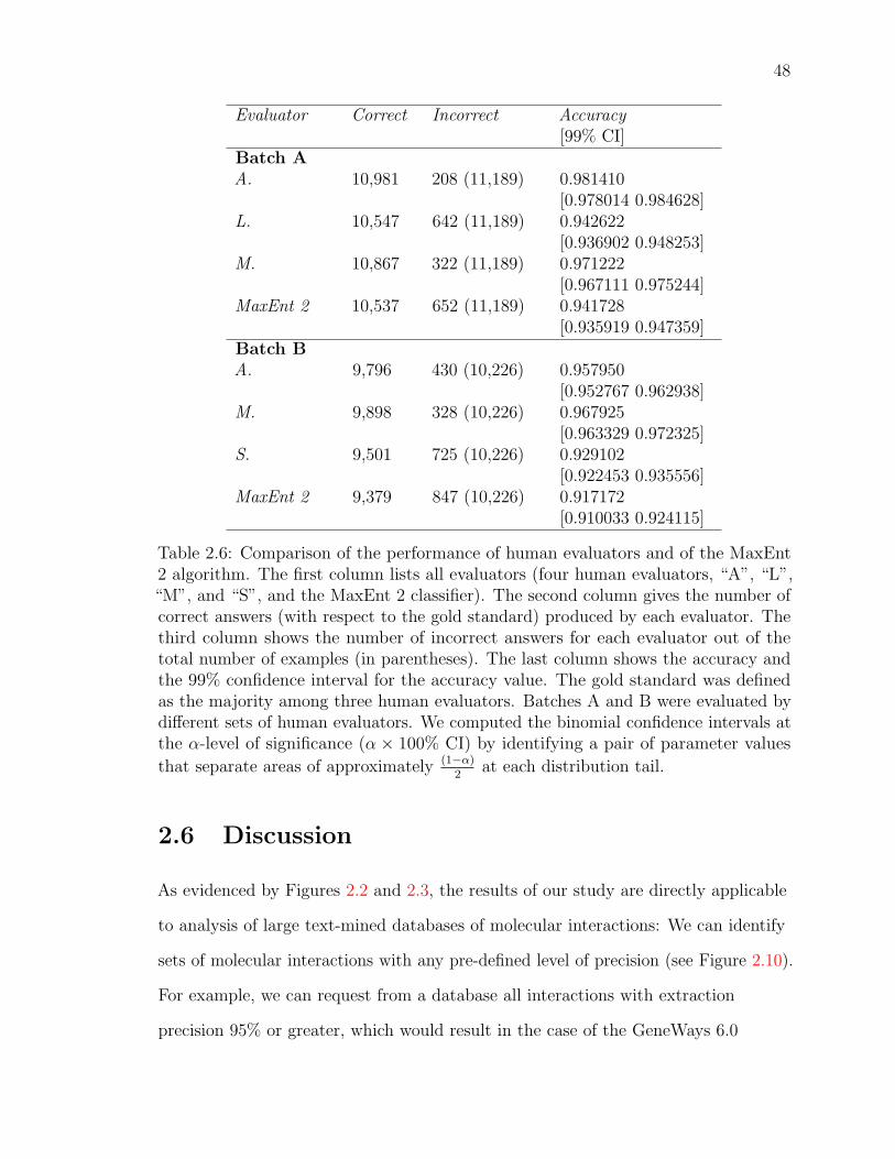
48
Evaluator Correct Incorrect Accuracy[99% CI]
Batch AA. 10,981 208 (11,189) 0.981410
[0.978014 0.984628]L. 10,547 642 (11,189) 0.942622
[0.936902 0.948253]M. 10,867 322 (11,189) 0.971222
[0.967111 0.975244]MaxEnt 2 10,537 652 (11,189) 0.941728
[0.935919 0.947359]Batch BA. 9,796 430 (10,226) 0.957950
[0.952767 0.962938]M. 9,898 328 (10,226) 0.967925
[0.963329 0.972325]S. 9,501 725 (10,226) 0.929102
[0.922453 0.935556]MaxEnt 2 9,379 847 (10,226) 0.917172
[0.910033 0.924115]
Table 2.6: Comparison of the performance of human evaluators and of the MaxEnt2 algorithm. The first column lists all evaluators (four human evaluators, “A”, “L”,“M”, and “S”, and the MaxEnt 2 classifier). The second column gives the number ofcorrect answers (with respect to the gold standard) produced by each evaluator. Thethird column shows the number of incorrect answers for each evaluator out of thetotal number of examples (in parentheses). The last column shows the accuracy andthe 99% confidence interval for the accuracy value. The gold standard was definedas the majority among three human evaluators. Batches A and B were evaluated bydifferent sets of human evaluators. We computed the binomial confidence intervals atthe α-level of significance (α × 100% CI) by identifying a pair of parameter values
that separate areas of approximately (1−α)2
at each distribution tail.
2.6 Discussion
As evidenced by Figures 2.2 and 2.3, the results of our study are directly applicable
to analysis of large text-mined databases of molecular interactions: We can identify
sets of molecular interactions with any pre-defined level of precision (see Figure 2.10).
For example, we can request from a database all interactions with extraction
precision 95% or greater, which would result in the case of the GeneWays 6.0

49
Evaluator Correct Incorrect Accuracy(Total) [99% CI]
Batch AA. 10,700 182 (10,882) 0.983275
[0.980059 0.986400]L. 10,452 430 (10,882) 0.960485
[0.955615 0.965172]M. 10,629 253 (10,882) 0.976751
[0.972983 0.980426]MaxEnt 2 10,537 345 (10,882) 0.968296
[0.963885 0.972523]Batch BA. 9,499 363 (9,862) 0.963192
[0.958223 0.967958]M. 9,636 226 (9,862) 0.977084
[0.973130 0.980836]S. 9,332 530 (9,862) 0.946258
[0.940276 0.952038]MaxEnt 2 9,379 483 (9,862) 0.951024
[0.945346 0.956500]
Table 2.7: Comparison of human evaluators and a program that mimicked their work. The firstcolumn lists all evaluators (four human evaluators, “A”, “L”, “M”, and “S”, and theMaxEnt 2 classifier). The second column gives the number of correct answers (withrespect to the gold standard) produced by each evaluator. The third column shows
the number of incorrect answers for each evaluator out of the total number ofexamples (in parentheses). The last column shows the accuracy and the 99%
confidence interval for the accuracy value. The gold standard was defined as themajority among three human evaluators and the MaxEnt 2 algorithm. Batches A andB were evaluated by different sets of human evaluators. We computed the binomialconfidence intervals at the α-level of significance (α× 100% CI) by identifying a pair
of parameter values that separate areas of approximately (1−α)2
at each distributiontail.
database in recall of 77.9%.12 However, we are not forced to discard the unrequested
12Recall is defined as number of true positivesnumber of true positives+number of false negatives . The false-negative results—the
facts that were in the original text but were missed by the system—can be generated at two stagesof the analysis. The first stage, information extraction, occurs when the GeneWays pipeline recoversfacts with recall β—we did not try to measure the value of β in the present study. The second stageis the automated curation of the database, during which all facts with score below a certain thresholdare discarded. This second stage is associated with an additional loss of the recall: Only a proportion,ρ, of the originally extracted true-positive facts is retained. It is the second type of recall that wediscuss in the text (see Figure 2.10). The overall recall, including both stages of the analysis, is justa product of the two values, βρ.

50
!1 0 10
1
Accuracy
Precision
Recall
Threshold
Figure 2.10: Values of precision, recall and accuracy of the MaxEnt 2 classifier plottedagainst the corresponding log-scores provided by the classifier. Precision is definedas true positives
true positives+false positives, recall is defined as true positives
true positives+false negatives, and accuracy is
defined as true positives+true negativestrue positives+true negatives+false positives+false negatives
. The optimum accuracy was
close to 88%, and attained at score threshold slightly above 0. We can improveprecision at the expense of accuracy: For example, by setting the threshold score to0.6702 we can bring the overall database precision to 95%, which would correspond toa recall of 77.91%12 and to an overall accuracy of 84.18%.
lower-than-threshold-precision interactions as we must the chaff separated from wheat
in the epigraph to this article. Intuitively, even weakly supported facts can be useful
in interpreting experimental results, and may gain additional support when studied in
conjunction with other related facts (see Figure 2.1 for examples of weakly supported
yet useful facts, the accuracy predictions were computed using the MaxEnt 2 method).
We envision that, in the near future, we will have computational approaches, such as
probabilistic logic, that allow us to use weakly supported facts for building a reliable
model of molecular interactions from unreliable facts (paraphrasing John von

51
Neumann’s “synthesis of reliable organisms from unreliable components” [100]).
Experiments with any standalone set of data generate results insufficient to allow us
to draw conclusions about the general performance of different classifiers.
Nevertheless, we can speculate about the reasons for the observed differences in
performance of the methods when applied to our data. The modest performance of
the Naıve Bayes classifier is unsurprising: We know that many pairs of features used
in our analysis are highly or weakly correlated (see Figures 2.8 and 2.5). The actual
feature dependences violate the method’s major assumption about the conditional
independence of features. MaxEnt 1, which performed significantly more accurately
than the Naıve Bayes in our experiments, but was not as efficient as other methods,
takes into account only the class-specific mean values of features; it does not
incorporate parameters to reflect dependencies between individual features. This
deficiency of MaxEnt 1 is compensated by MaxEnt 2, which has an additional set of
parameters for pairs of features leading to a markedly improved performance.13
Our explanation for the superior performance of the MaxEnt 2 algorithm with respect
to the remainder of the algorithms in the study batch is that MaxEnt 2 requires the
least parameter tweaking in comparison to other methods of similar complexity.
Performance of the Clustered Bayes method is highly sensitive to the definition of
feature clusters and to the way we discretize the feature values—essentially presenting
the problem of selecting an optimal model from an extensive set of rival models, each
model defined by a specific set of feature clusters. Our initial intuition was that a
reasonable choice of clusters can become clear from analysis of an estimated
feature-correlation matrix. We originally expected that more highly correlated
parameters would belong to the same cluster. However, the correlation matrices
estimated from the complete GeneWays 6.0 database and from a subset of annotated
13We also analyzed the relation between the size of the training data set and the accuracy ofMaxEnt 2 method. While accuracy of the MaxEnt 2 method with the whole training data set was87.97%, it dropped to 87.38% when using only 60% of the training data, and to 83.57% with 20% ofthe training data.

52
facts turned out to be rather different—see Figure 2.5—suggesting that there are
conflicting groups of highly correlated features. In addition, analysis of mutual
information between the class of a statement and pairs of features (see Figure 2.8)
indicated that the most informative pairs of features are often only weakly correlated.
It is quite likely that the optimum choice of feature clusters in the Clustered Bayes
method would lead to a classifier performance accuracy significantly higher than that
of MaxEnt 2 in our study, but the road to this improved classifier lies through a
search in an astronomically large space of alternative models.
Similar to optimizing the Clustered Bayes algorithm through model selection, we can
experiment with various kernel functions in the SVM algorithm, and can try
alternative designs of the artificial neural network. These optimization experiments
are likely to be computationally expensive, but are almost certain to improve the
prediction quality. Furthermore, there are bound to exist additional useful
classification features waiting to be discovered in future analyses. Finally, we
speculate that we can improve the quality of the classifier by increasing the number of
human evaluators who annotate each data point in the training set. This would allow
us to improve the gold standard itself, and, with luck, would lead to develop a
computer program that performs the curation job consistently at least as accurately
as an average human evaluator.

53
Method ROC score ± 2σClustered Bayes 68 0.8115± 0.0679Naıve Bayes 0.8409± 0.0543MaxEnt 1 0.8647± 0.0412Clustered Bayes 44 0.8751± 0.0414QDA 0.8826± 0.0445SVM-t0 0.9203± 0.0317SVM 0.9222± 0.0299Neural Network 0.9236± 0.0314SVM-t1-d2 0.9277± 0.0285SVM-t2-g2 0.9280± 0.0285SVM-t1-d3 0.9281± 0.0280SVM-t2-g1 0.9286± 0.0283SVM-t2-g0.5 0.9287± 0.0285MaxEnt 2 0.9480± 0.0178MaxEnt 2-v 0.9492± 0.0156
Table 2.8: The receiver operator characteristic (ROC) scores (also called the area underthe ROC curve) for methods used in this study, with error bars calculated in 10-foldcross-validation. We evaluated the Meta-method on a smaller set of data, so did notinclude its results in this Table. (The estimated ROC score for the Meta-methodwas 0.9456 ± 0.0076; it performed better than MaxEnt 2 in each cross-validationexperiment, data not shown).
54
Chapter 3
Overview of biomedical term
recognition and classification
3.1 Introduction
The term recognition and classification project was designed to address shortcomings
in GeneWays that were identified in the curation project described in Chapter 2. One
of the findings was that terms that were not reliably recognized produced a decrease
in the performance of GeneWays. The goal, then, was to improve on the term tagging
[55] and disambiguation [59] stages of the current GeneWays version to improve
results. The framework followed was that proposed by Krauthammer and Nenadic
[101], which divides the term identification task into three stages: term recognition,
term classification, and term mapping. This introduction will present the previous
work in term recognition and classification that influenced the project described in
Chapter 4, with special focus on biomedical applications.

55
3.1.1 Term recognition
Automatic term recognition (ATR) grew from the fields of information retrieval (IR)
and indexing [102]. The goal of indexing was to improve IR searches by focusing
them on a limited number of surrogate descriptors instead of on full document text.
The surrogates often were lexical units—like words of a certain type—that were used
to build an index representing a document. Thus, searches could be centered on
selected relevant words instead of all words. This approach is similar conceptually to
the keywords included in library index cards. For example, a classical automatic
indexing technique is to exclude from an index words that are too frequent (also
called stop words, like the, a, and of ), which do not add discriminatory power to a
search because most documents include them. The first work in automatic indexing
dates back to the late 1950s [103]. Early automatic indexing work is based on
single-word index keywords. At the beginning of the 1970s the first multi-word
expression indexes are developed.
ATR is a natural continuation for indexing. In its simplest expression, it brings an
additional restriction to the task: that the surrogates extracted from a document
belong to a specific domain. It is in the context of ATR that terms are used for
indexing [104], and one of the early focuses of ATR was specialized terminologies
created automatically from text. ATR overcomes limitations in single-word automatic
indexing. Many objects or concepts often are written using more than one word (e.g.,
“United States of America”), if indexing is limited to single words (“United”, “States”,
“of”, or “America”) important information is lost. Multi-word indexing that is not
based on terms has its pitfalls, though, such as identifying groups of words of
uncertain value. In multi-word indexing there might be little conceptual difference
between using “States of America” or “United States of America” as the index, but
clearly the two expressions are of different usefulness. Terms are important because
they are semantically loaded and thus allow for more effective retrieval given the

56
semantic interests typically expressed in many searches (e.g., retrieve all documents
that deal with “network engineering”). Terms are understood as expressions that may
be included in a specialized terminology—a vocabulary relative to a domain.
The two main approaches to ATR have been statistical and linguistic. Statistical
approaches rely on analysis of the tendency of words to appear next to, or separate
from, each other, in the same document or in different documents, and within certain
grammatical settings (e.g., as adjective + noun). For example, the fact that two
words appear next to each other more often than expected (a bigram) may hint that
they belong to the same term. Linguistic approaches rely on the grammatical and
syntactical patterns that appear in term formation. These patterns point out
relationships among words that together may form a term. The noun phrase is
considered a basic unit for term analysis (an example of noun phrase: “the red horse
car”); it is a syntactic unit typically organized around a noun (the head noun, in this
case, “car”). The words that are members of a noun phrase are modifiers of the head
noun. These words often are adjectives (“red”), determinants (“the”), or other nouns
(“horse”) that appear beside the head noun. Noun phrases can be determined by
syntactic parsing. Linguistic and statistical analyses can be combined for improved
results.
3.1.2 Named entity expressions
The pioneering Message Understanding Conference (MUC) series sponsored by
DARPA between 1987 and 1997 aimed to improve information extraction methods by
presenting different tasks open to competition. The format of the competitions
encouraged the standardization of evaluation that has become more and more
commonplace in computational linguistics. A named entity task was presented in
MUC-6 in 1995 [105, 106] and, again, in MUC-7. The challenge was to recognize
three different expression types in a corpus: temporal expressions (date); number

57
expressions (money, percent); and entity names. The contenders were scored on
correct and partial matches to generate an overall score. The entity name recognition
subtask involved recognition of names of people, organizations, and geographic
locations. In the context of MUC-6 and MUC-7, entity name referred to what is more
commonly called a proper name (e.g., Coca-Cola, James, Hollywood) [107]. This
subtask became popularized as named entity recognition (NER) and its meaning was
generalized to be recognition of any terms of interest, not necessarily the ones that
are usually understood as being proper names 1. NER combined term recognition and
classification into one subtask, which not only brought together techniques from both
fields but also spawned a new breed of studies. MUC’s NER promoted further work
in term recognition and classification in other domains and applications, such as the
multilingual entity task workshops (MET-1 and MET-2) [108]. One of the
innovations of MUC’s NER was the scoring competition model using a tagged corpus
as gold standard, which was replicated later in other competitions such as
BioCreAtIvE I and II [69]. Its success—and perhaps its demise—was the high level of
accuracy attained, which made it possible to declare the subtask “solved”, with an
F-measure score of 94%− 97% [107].
3.1.3 Term classification
Term classification has received much less attention than term recognition. The first
work in the field, which dates to the late 1960s and early 1970s [109, 110, 111], was
devoted to classifying indexing keys to improve information retrieval. The task was
named “automatic term classification”, which was akin to its sibling “automatic term
recognition”.
1Discussing the philosophical meaning of “proper name” is outside of the scope of this text, but asimple rule of thumb might be the uniqueness implied by a proper name. For example, “horse” is acommon name while “Bucephalus”, Alexander The Great’s horse, is a proper name. Protein namesdo not seem to conform, generally, to this uniqueness constrain. Moreover, notice that, in English,proper names are often capitalized (though you may consider exceptions like the poet name “e.e.cummings”).

58
While word sense disambiguation (WSD) might be considered a term classification
subtask, or at least a type of term classification, it has a much older pedigree that
dates to the dawn of computational linguistics because of its applications in machine
translation or information retrieval [112]. As a result, many of the features and
techniques used in WSD were used later for term classification [113, 114]. Features
used include [114]:
1. Part of Speech (POS).
2. Morphology.
3. Collocations.
4. Semantic word associations.
a. Taxonomical organization.
b. Situation.
c. Topic.
d. Argument-head relation.
5. Syntactic cues.
6. Semantic roles.
7. Selectional preferences.
8. Domain.
9. Frequency of senses.
10. Pragmatics.
59
New interest in term classification arose with the inception of the NER task. The
classes included in MUC-6 were carefully defined to avoid ambiguities, like
distinguishing when “White House” belongs to the class ENTITY or the class
LOCATION. Features for classification where devised that were included along others
for boundary recognition. The field has often been called named entity classification
(NEC), even if it does not always deal with named entities; this is the same thing
that happened with term recognition.
Since MUC’s NER originated, term classification has gone in several directions:
• Term recognition and classification
Term classification that goes hand-in-hand with term recognition, tackling
NER-style problems.
• Term classification
Separated from term recognition if, maybe, using training/testing examples
from the same NER corpora but devising two independent tasks [115, 116, 117].
– Large-scale
With classes sometimes numbering in the hundreds, evaluation is of a
different nature and is oriented towards population of large ontologies
[118, 119, 120].
– Sub-categorization
Also called fine-grained classification (e.g., dividing the term class
PERSON into the classes ATHLETE, POLITICIAN/GOVERNMENT,
CLERGY, BUSINESSPERSON, ENTERTAINER/ARTIST, LAWYER,
DOCTOR/SCIENTIST, and POLICE [121, 122, 123]).
The relative indifference in research towards term classification outside named entities
might come from the fact that the domains commonly involved in the NER tasks do

60
not have such a rich and evolving vocabulary as does the biomedical domain. There
is not a strong need for term classification in situations where most terms are present
in dictionaries. Outside proper nouns, only domains such as chemistry, biology, or
medicine have dictionaries or terminologies that are rendered quickly obsolete and
inflexible by the fast-paced creation of new terms and term variations.
3.1.4 Biomedical term recognition and classification
NER’s influence on biomedical information extraction appeared in 1998 [124]. Given
the lack of previous work in biomedical term recognition 2 and classification and the
groups that began to work on it, it seems likely that text mining was a main driving
force behind this growth. Although many researchers have used the term NER in
their projects, this has been a misnomer (see for example the use of “Bio-NER” in
[126]) and a legacy of MUC influence. Term recognition and classification in
biomedicine is similar to NER in that it attempts to recognize and classify a limited
number of classes (but usually just one) in a corpus. Unlike NER, however, it does
not deal with proper nouns but with terms. This narrow focus produces precisely
class-tailored strategies for different term classes.
Another influence from MUC’s NER is that the number of tagged corpora available,
at least for molecular biology, has been increasing (e.g., Genia [127], Yapex [128]),
and competitions such as the Bio-Entity Recognition Task in the Joint Workshop on
Natural Language Processing in Biomedicine and its Applications (JNLPBA) [129],
and the Critical Assessment of Information Extraction in Biology (BioCreAtIvE-1
(2004) and BioCreAtIvE-2 (2006), both with their own corpus) workshop [130].
Biomedical term recognition has adopted many of the techniques used in MUC’s
NER [131, 132], including a fusion of the term recognition and classification stages
(what Lee and colleagues called “one-phase NER” [133]). However, the differences
2A pre-NER biomedical term recognition study like [125] is so different to posterior work that itshows how influential NER became.
61
prompted Takeuchi and Collier [134] to call it “extended named entity task (NE+).”
Work in term recognition and classification that predates MUC’s NER approach has
been influential for biomedical term recognition as well (see, for example, the
similarities between [135] and [136]).
While some researchers have declared NER to be solved, this is not the case for
biomedical term recognition and classification (e.g., “Although named entity
recognition might be regarded a solved problem in some domains, it still poses a
significant challenge in others.” [128]). The proper names considered in MUC’s NER
are more limited in variation compared to biomedical terminology. The vocabulary in
the biomedical domain is formidable [137], open [138] and growing; few rules are
followed [124]; term variability is high [139]; no established rules exist for term
boundary definition3 [140, 141], and class ambiguity is higher than in other domains
[132]. Perhaps the best proof of its higher complexity is that MUC algorithms
adapted to biomedical text have produced lower results.
Biomedical term recognition and classification faces terminology issues such as:
“For example, there is a gene name “bride of sevenless” (FlyBase IDFBgn0000206) with its acronym “boss”, as well as a protein that has beennamed after a Chinese breakfast noodle “yotiao” (Swiss-Prot ID Q99996).Even if biologists start to use exclusively “well-formed” and approvednames, there are still a huge number of documents containing “legacy”and ad hoc terms.” [101]
“For example, we have fourways to tag the name in the phrase ‘yeastYSY6 protein’: ‘yeast YSY6 protein’, ‘yeast YSY6’, ‘YSY6 protein’ or‘YSY6’. This ambiguity implies that annotators may include yeast todayand may exclude it a year later, unless given some ‘annotation rules’. [...]
To make things worse, protein names are often derived from descriptiveterms (signal transducer and activator of transcription, STAT) and only
3There is an on-going effort in defining how term boundaries should be set for certain biomedicalterm classes at the European Bioinformatics Institute, called “A framework for named entityannotations and interoperability of text mining components.” The effort is led by the Rebholz group.
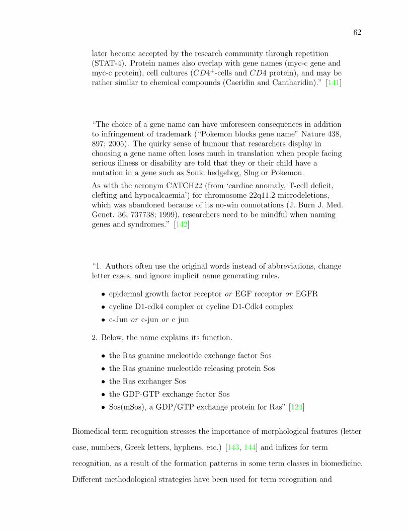
62
later become accepted by the research community through repetition(STAT-4). Protein names also overlap with gene names (myc-c gene andmyc-c protein), cell cultures (CD4+-cells and CD4 protein), and may berather similar to chemical compounds (Caeridin and Cantharidin).” [141]
“The choice of a gene name can have unforeseen consequences in additionto infringement of trademark (“Pokemon blocks gene name” Nature 438,897; 2005). The quirky sense of humour that researchers display inchoosing a gene name often loses much in translation when people facingserious illness or disability are told that they or their child have amutation in a gene such as Sonic hedgehog, Slug or Pokemon.
As with the acronym CATCH22 (from ‘cardiac anomaly, T-cell deficit,clefting and hypocalcaemia’) for chromosome 22q11.2 microdeletions,which was abandoned because of its no-win connotations (J. Burn J. Med.Genet. 36, 737738; 1999), researchers need to be mindful when naminggenes and syndromes.” [142]
“1. Authors often use the original words instead of abbreviations, changeletter cases, and ignore implicit name generating rules.
• epidermal growth factor receptor or EGF receptor or EGFR
• cycline D1-cdk4 complex or cycline D1-Cdk4 complex
• c-Jun or c-jun or c jun
2. Below, the name explains its function.
• the Ras guanine nucleotide exchange factor Sos
• the Ras guanine nucleotide releasing protein Sos
• the Ras exchanger Sos
• the GDP-GTP exchange factor Sos
• Sos(mSos), a GDP/GTP exchange protein for Ras” [124]
Biomedical term recognition stresses the importance of morphological features (letter
case, numbers, Greek letters, hyphens, etc.) [143, 144] and infixes for term
recognition, as a result of the formation patterns in some term classes in biomedicine.
Different methodological strategies have been used for term recognition and

63
classification ranging from straightforward dictionary matching to black box setups
based on machine learning. Here they are described separately, although they more
commonly are used in conjunction.
Dictionary matching
Matching dictionary entries to text is a simple method for term recognition and
classification. The coverage limitations of this method are familiar: Dictionaries have
gaps, they do not keep pace with the state-of-the-art, and they do not record term
variation properly. Dictionaries also have limited in precision because a partial match
does not ensure a true positive. Moreover, they are not helpful for disambiguation.
Dictionary matching is used more often for feature generation rather than for term
recognition technique, as explained in Section 3.1.4.
An improvement over simple matching is increasing the matching flexibility to some
extent 4. Dictionary matching can be combined with additional information for
improved matching (see, for example, [46]). Krauthammer and colleagues [55] used
an innovative approach to matching using a BLAST-inspired algorithm [54] that
performs short matches between the text and dictionary terms. These matches are
later extended to find the matches that lie above a certain significance threshold.
Morgan and colleagues [145] used suffix tree and longest-extent pattern matching on
filtered abstracts similar to [146]. Yamamoto and colleagues instead used morphemes
as basic units for matching [147].
Syntax
A syntactical model of term recognition and classification is very helpful in reducing
the search space and anchoring term words. Strategies used are influenced by previous
term recognition work (see Section 3.1.1) in part of speech tagging and shallow
4This analogous to pattern matching techniques described in Section 3.1.4.

64
parsing, but not in deep parsing. Noun phrases [131] and head nouns [148] sometimes
are used as term placeholders or anchors. POS tags are integral features of many
models, including Markov-based machine learning models ([143], see Section 3.1.4).
Models based on “core terms” are a departure from non-biomedical term recognition
and classification models. Originally proposed by [124], core terms are words that
contain capital letters, numerical figures, and special symbols characteristic of protein
names. Terms are reconstructed around the “core terms” following several rules.
Hanisch and colleagues [149] proposed a more elaborated model (see Table 3.1).
Name Description ExamplesModifier Semantic-modifying tokens receptor, inhibitorNon-descriptive Annotating tokens fragment, precursorSpecifier Numbers and Greek letters 1, V1, alpha, gammaCommon Common English words and, was, killerDelimiter Separator tokens ( ) , . ;Standard Standard tokens TNF, BMP, IL
Table 3.1: Definition of token classes with differing semantic significance [149].
Syntactical strategies can be used in conjunction with additional features to filter
terms that are not of interest.
Rule-based methods, probabilities and statistics
The first method used in biomedical term recognition was a rule-based recipe of steps
for recognizing genes and proteins on the SH3 domain and signal transduction
abstracts [124]. Although results were good, this technique’s lack of flexibility led to
other efforts to make it more general [128, 150]. The steps involved a syntactic model
that was increasingly refined with statistics and probability filtering. Hou and Chen
[151] used collocation statistics to enhance the results in [124] and [128]. A
suffix-matching and extension rule-based grammar was used by [152, 145].
Nobata and colleagues [131] used a probability method based on Naıve Bayes (see
Section 2.4.1 on Naıve Bayes) and decision trees for term classification. Tanabe and
65
Wilbur used Naıve Bayes with different statistical and POS features [153, 154]. For
word sense disambiguation (see Section 3.1.4), Hatzivassiloglou and colleagues [59]
opted for three different methods: Naıve Bayes learning, decision trees, and inductive
rule learning.
Machine learning
Several machine learning techniques have been used in the context of biomedical term
recognition and classification. While techniques based on sequential state chains
might be considered a better fit for a task involving sequential word tokens, support
vector machines (SVMs) have been applied more often
([155, 156, 148, 133, 141, 157, 158], see Section 2.4.1). The common problem facing
SVM implementation is that the data are very unbalanced—a given text contains
many more words that do not belong to a term than words that do. To address this
issue, different filtering methods have been used to reduce the search space, they
eliminate words that are not part of a term using POS information, dictionaries, or
n-gram statistics, and other information that represents a syntactic understanding of
terms. The post-processing counterpart of filtering is extension, which consists of
recovering words that may have been erroneously filtered to reconstruct terms. A
SVM method without filtering/extension also has been implemented using a sliding
window [157].
The prediction model for SVMs is based on B/I/O notation that is typical of simple
sequential Markov models. Words that do not belong to a term are labeled O,
whereas words that belong to a term are labeled B or I followed by the class. B
stands for the first word of a term and I for an intermediate word. For example, the
sequence “accurate initiation of transcription by RNA polymerase II”, can be labeled
for the class protein as “accurate/O initiation/O of/O transcription/O by/O
RNA/B-PROTEIN polymerase/I-PROTEIN II/I-PROTEIN” [133].

66
Sequential Markov model machine learning algorithms such as hidden Markov models
([159, 145, 160, 161], see Section 3.2), maximum entropy Markov models (MEMM)
([162, 156], see Section 2.4.1 on maximum entropy), and conditional random fields
([163, 164, 126, 165], see Section 3.2) are a closer fit for addressing the task, although
they also face the difficulties posed by an unbalanced label sequence. A different
approach is integrating different models [166].
Word sense disambiguation
WSD has been closely linked to term classification. WSD is necessary in instances
where a term belongs to two or more classes or terminologies. Because morphological,
infix, and string matching features do not differ between ambiguous terms, deciding
which class is the correct one entails contextual analysis. WSD has a long tradition in
natural language processing (see also Section 3.1.3), and this tradition has been
adapted to biomedical text in recent times
[167, 59, 168, 169, 170, 171, 132, 172, 173, 174]. There is even a biomedical corpus
specialized in WSD [175]. As pointed out in [59, 132, 176], WSD is a harder task in
biomedical texts compared to other texts such as news feeds; the principle of “one
sense per discourse” does not hold as strongly in the former [132]. Gale and
colleagues proposed the concept of “one sense per discourse” in an influential study of
the persistence of a word sense of an ambiguous word in a text [177]. They discovered
that in 98% of cases ambiguous words were used in only one sense within a text. This
finding has been very influential, although it also has been criticized for their use of
disambiguation categories that were too coarse-grained [178]. Another study
quantified sense persistence in a text to be about 70% [179] for finer-grained
categories. In biomedical text, sense persistence has been estimated to be 60% [132].
“The biology domain offers a prime example of this multiplicity ofmeanings, since every protein has an associated gene with often the same
67
name. Further, genes and their transcripts (mRNA, rRNA, tRNA and thelike) often share the same name as well. Often an article will refer to theprotein, gene, and RNA senses of a term in close proximity, relying on thereader’s expertise and the surrounding context for disambiguation. Forexample, SBP2 is listed as a gene/protein in the GenBank [...] database.In one of our source articles [...] we find the following sentences:
• ‘By UV cross-linking and immunoprecipitaion, we show that SBP2specially binds selenoprotein mRNAs both in vitro and in vivo.’
• ‘The SBP2 clone used in this study generates a 3173 nt transcript(2541 nt of coding sequence plus a 632 nt 3’ UTR truncated at theplyadenylation site).’
In the first sentence the highlighted occurrence of SBP2 is a protein, whilein the second sentence is a gene.” [59]
Moreover, in the biomedical domain word sense might be harder for humans to
distinguish. The pairwise agreement between human annotators for classification of
gene and protein names has been measured to be about 78% [59, 176], compared to
88− 100% for generic word senses [180, 176].
Abbreviation or acronym resolution is a special case of WSD, for which a specific set
of techniques has been developed [181, 182, 183, 184, 185, 186, 187]. The processing
entails mapping an abbreviation to a definition for the purpose of disambiguating its
meaning. Definitions and abbreviations may appear appositionally (e.g., the
abbreviation DNA and the definition desoxyribonucleic acid in: Deoxyribonucleic acid
(DNA)), but abbreviations may be found anywhere in a text, as definitions commonly
are written only the first time the abbreviation is used. A third case occurs when the
author considers that an abbreviation is so well known within a scientific field (e.g.,
DNA) that the definition is unnecessary, in this case it must be searched in a different
text.
Although abbreviation resolution faces challenges similar to those of other biomedical
text-mining tasks (e.g., large, open vocabulary; few rules; plurality of domains), it
actually is a success story and almost a solved problem. This is, perhaps, because it
is a well-defined task in terms of inputs and outcomes. Okazaki and Ananiadou [185]

68
reported 99% precision and 82− 95% recall. Yu and colleagues [187] reported 92%
precision and 91% coverage.
Features for machine learning
Two studies have shown how classical features compare in helping to classify and
recognize term classes [144, 188]. Torii and colleagues [144] enumerated four common
feature types:
1. F-term: Fukuda and colleagues [124, 128] proposed the use of functional terms
(F-terms), which are words that immediately follow a term and represent a
strong clue to deciding its class and one of its boundaries (e.g., in “EGF
receptor”, the word “receptor” indicates that EGF is a protein). First efforts
were based on lists of manually selected F-terms but automatic, probabilistic
approaches were developed later [144, 148]. F-term is a particular case of a
contextual feature. Its popularity is perhaps driven by its power and simplicity
to be characterized and codified. Rindflesch and colleagues [46] talked more
broadly of signal words, such as cell, clone, line, and cultured for the class cell
and activated, expression, gene, and mutated for the class gene.
2. Suffix: Suffixes are especially useful for classes in which word endings have
standard meanings associated with them. This is often the case with chemical
names (e.g., -ose, -ide, -ite, -ate) or protein names (e.g., -ase) [144]. Suffix is a
particular case of a substring feature, which would include prefix and infix.
3. String matching: Matching a sequence of words to an entry in a specialized
dictionary (or terminology) can give a strong clue about the term’s class (e.g.,
finding that a term is the name of a protein in the protein database SwissProt).
Dictionary lookup, however, has limitations for term matching for several
reasons (see also Section 3.1.4). One of them is that small variations in a term’s
69
form may hamper recognition (e.g., alpha-glucose vs. a-glucose). To avoid this,
more flexible matching algorithms have been devised, using a mixture of
features for similarity scoring. A comparison of matching algorithms can be
seen in [189, 190].
4. Context: Context is generally understood to mean the words that surround a
term in the text where the term appears. Often, context is limited to a window
of several words that precede and follow a term. Context has been shown to be
a powerful indicator of a term class, as the words used tend to differ in the
surroundings of a given term depending on its class [191] (e.g., the verbs used
are different [192]).
Character-level (also known as ortographical or morphological) features are another
important type of features. This is a motley set of features about a term’s form that
can often be encoded with binary values and have the potential to differentiate terms
that belong to different classes. No established list of common morphological features
exists, but similarities abound in the choices researchers make. Table 3.2 shows an
example of a list used by [143]. Morphological, infix, and string matching features
have been called internal evidence [193] (or word-internal information [194]), unlike
F-terms and other contextual information, which are called external evidence.
3.2 Mathematical Background
3.2.1 Recognition and classification framework
The classification framework presented in Section 2.4.1 must be extended to address
sequential and multi-class assignation problems. Our sequential problem involves a
sequence of tokens t1, t2, . . . , tn with feature associated vectors F1,F2, . . . ,Fn, for
which we identify subsequences Tk = (ti, ti+1, . . . , tj) that are potential terms. These

70
Feature ExampleGreekLetter kappaCapsDigitHyphen Oct-1CapsAndDigits STAT1SingleCap BLettersAndDigits p105LowCaps pre-BIOneDigit 2TwoCaps EBVInitCap SoxHyphenDigit 95-LowerCase kinasesHyphenBacklash -Punctuation (DigitSequence 98401159TwoDigit 37FourDigit 1997NucleotideSequence
Table 3.2: Morphologic binary feature values with examples as used in [143]. Althoughno single list of agreed-upon features exists, they tend to overlap and are tuned forsimilar cues depending on the term classes being considered.
subsequences might be arranged in a nested fashion. A term Tk is nested when all of
its tokens are included in another term Tl, or
∃l | Tk ⊂ Tl. (3.1)
A term Tk is a parent if it is not nested, namely,
@l | Tk ⊂ Tl. (3.2)
We break down the sequential task into two parts: identifying parent terms, and
identifying nested terms. As explained in Section 4.2.3, our approach is to filter
tokens by considering only those that are part of noun phrases. Some filtered tokens
are reconsidered afterwards when joining noun phrases. For parent terms, tokens are
classified into the classes cterm and cnon−term, with the labels I and O, respectively.
71
Nested tokens may present themselves in more complex arrangements, and hence the
list of labels is longer:
• B : beginning of term
• I : intermediate
• E : end of term
• U : unary (one-token) term
• UE : unary term and end of term
• UB : unary term and beginning of term
• O : non-term
The label U also is used in place of a label UI. The subsequences identified as
potential terms are considered further for the semantic class assignation problem. A
potential term Tk might be classified into a term class ci that belongs to a set of
classes C,
C = (c1, c2, . . . , cn). (3.3)
Potential terms that are not assigned to a class in C are assigned to the class cother.
Hence, the class cother changes in scope depending on the class set C. The set of all
terms in a sentence is defined by a vector T , while the set of classes assigned to the
terms in T is defined by a vector C.
3.2.2 Conditional random fields
Conditional random fields (CRF) [195, 196] is a machine learning technique (in
addition to those presented in Section 2.4.1). It is a type of graph probabilistic model

72
that has been proved to be very suitable for sequential problems. CRF builds on
Markov random fields theorems. To visualize Markov random fields, consider a lattice
system (a graph) of mutually interdependent random variables. The Markov property
allows us to model how a variable is influenced by all the other variables by
considering only its immediate neighbors. More formally, for a set of variables C, the
ith variable Ci is surrounded by a neighborhood of variables CS. The conditional
probability distribution of Ci can be described as
p(Ci | C) = p(Ci | CS), (3.4)
where CS,Ci ⊂ C [197, 198]. Exponential distributions are a set of functions that are
amenable for Markov random field modeling and that minimize assumptions over the
system (see Section 2.4.1). Equation 3.4 can be thus rewritten as
p(Ci | CS) =1
Zexp
∑Cj∈CS
λj
, (3.5)
where Z is a normalization factor that makes the distribution sum equal to one.
In the case of CRFs, the neighbor relationships are defined by the interdependencies
between features and classes. Intuitively, the class of a token 5 within a sentence is
strongly related to the class of the nearby tokens. Given that a sentence easily
resembles a chain graph structure, we could redefine Equation 3.5 to capture the
dependencies between the tokens in a sentence and its features. A linear-chain
conditional random field can be defined as
p(Ci | F) =1
Zexp
(K∑k=1
λkfk(cj, cj−1,Fj)
), (3.6)
where Z is
5Token is used as a more general term than word but in many cases it is interchangeable.
73
Z =∑C
exp
(K∑k=1
λkfk(cj, cj−1,Fj)
). (3.7)
The index j refers to the members of the vector C, and the index k to the members of
the vector F . The feature functions fk(cj, cj−1,Fj) define the dependencies. Feature
functions are, in our case, simple indicator functions that are equal to 1 for selected
variable combinations,
fk(cj, cj−1,Fj) = 1{j=k}. (3.8)
Solving the linear-chain conditional random field entails estimating the parameters,
θ = {λk}.

74
Chapter 4
Biomedical term recognition and
classification using large corpora
and search engines
4.1 Introduction
As explained in Section 3.1.2, most work in term recognition and classification is
based on the named entity recognition (NER) task from the Message Understanding
Conference 6 and 7 (1995 and 1997). The task blended both term recognition and
term classification for systems specialized in extraction of terms from a specific
number of classes. This was a departure from early work that separated both tasks,
as explained in Sections 3.1.1 and 3.1.3. The NER approach has its own problems as
it offers little flexibility in the number of classes that can be recognized. For example,
with this approach algorithms are specifically tuned to the features that are more
likely to identify a class (e.g. suffixes for recognizing chemical terms). If term
recognition and classification are performed at the same time, little leeway is left for
multi-class classification other than running different term recognizers/classifiers

75
sequentially over a text. Perhaps as a result, most work in term
recognition/classification has been limited to at most five classes (notably, work
presented at the Joint Workshop on Natural Language Processing in Biomedicine and
its Applications [129]), and very often to single-class recognition/classification.
Gaizauskas and colleagues [152] used 12 sub-cellular classes with a small
training/testing set and hand-crafted rules. Other, existing proposals for more than
five classes are low-performing [156, 160, 133].
Krauthammer and Nenadic [101] presented a framework for term identification in
biomedicine that consists of three parts: (1) term recognition, (2) term classification,
and (3) term mapping. A system that follows this framework and completely
separates each stage could exchange parts like a layered architecture with interfaces
for communication. The term recognition stage should be able to recognize all
potential terms, in the spirit of the study with named entities by Black and
Vasilakopolos [116] 1. Two studies have experimented with separating term
recognition and classification with biomedical text [133, 199], with the argument that
features of importance are usually different for term recognition and term
classification.
For true multi-class recognition and classification the system should have a high
performance level and work well with new words without necessarily using
dictionaries (as noted by Mika and Rost [141]). For term recognition, the main hurdle
would be the definition of term boundaries, as they could prove to have variable
properties depending on the term class. For term classification, the classifier should
be flexible enough to adapt to any classes required by the task at hand, whether it is
a single-class or a > 30-class problem. Machine learning classification provides higher
flexibility that rule-based methods or probabilistic methods.
The following is an example of rule-based classification:
1This is an easier task than identifying all terms, as explained in Chapter sec:introduction2.

76
“Animals can be divided into:
a. belonging to the Emperor
b. embalmed
c. trained
d. pigs
e. sirens
f. fabulous
g. stray dogs
h. included in this classification
i. trembling like crazy
j. innumerable
k. drawn with a very fine camelhair brush
l. et cetera
m. just broke the vase
n. from a distance look like flies.” 2
We would prefer a system with more flexibility, like a machine learning approach.
Additionally, we would like our system to have other characteristics that we have
tried to implement:
• The performance limits of term classification should be limited by the
separability of the semantic spaces [202]. This is simply stating that we want
our classifier to be as good as possible.
• Term boundaries and classes should be defined by examples. The examples
would define both the dimensions of the semantic space and of the syntactic
space3. The syntactic space comprises the space that defines horizontal token
relationships such as term boundaries. This is simply stating that terms are in
2Chinese encyclopedia, “The Celestial Emporium of Benevolent Knowledge”. Translation byFranz Kuhn. The quote is in an essay by Jorge Luis Borges [200]. There is no other known referenceto this encyclopedia and this has fueled speculation that is a fictional quote even if Borges’s essay is,otherwise, non-fiction. A famous reference to this quote is by Michel Foucault in “Les Mots et leschoses: Une archeologie des sciences humaines.” [201].
3In its second entry, Merriam-Webster dictionary defines the word syntax as: “A connected ororderly system : harmonious arrangement of parts or elements ‘the syntax of classical architecture’ ”

77
the eye of the beholder: There are no rules set in stone for term boundaries or
semantic class. Defining terms is a contingent task and therefore examples are a
natural basis for a flexible approach.
4.2 Term recognition
4.2.1 Text pre-processing and indexing
In our system, text is tokenized and tagged for POS with Medpost [203], a highly
accurate tagger adapted to biomedical text, with an F-measure of 97% in Medline
abstracts. We performed shallow parsing for noun phrase information using YamCha,
the winner of the CoNLL 2000 Shared Task, Chunking [204], which has a reported
F-measure of 94% (after tagging and chunking).
Different corpora were used for statistical and context analysis. The corpora include
were the BioMed Central corpus of articles, GeneWays articles, Wikipedia, the
Reuters corpus, and the Medline abstracts, for a total of more than 150 million
sentences. Every corpus was processed for sentence boundaries, tagged, and chunked.
Sentences were indexed using the open source Apache Lucene technology from the
Apache Software Foundation [205]. Although only the sentence text was indexed,
additional information such as POS tags and shallow parsing was stored along with
the indexed sentences for quick retrieval. Once the sentences are indexed they can be
quickly retrieved performing queries using Lucene, similarly as it is done in
commercial search engines like Yahoo! or Google. The two main advantages of
indexing and searching for our analysis are that: (1) it allows for fast n-gram and
statistical computation for phrases of any size n, and (2) it can retrieve contextual
information for any text. With the large amount and breadth of sentences that we
indexed, the search engine can access contextual information for many term types
and variants and thus can provide a quick snapshot of term usage in real text.

78
4.2.2 Syntactical model
The approach used is to learn the structure of terms within noun phrases from
examples in the biomedical corpus GENIA V3.02 [127, 206] and then apply this
structure to any noun phrase, whether or not it has a GENIA term in it. In some
sense we are modeling a meta-term, or term boundary definition, that allows us to
predict term boundaries regardless of class: a class-independent, example-based term
boundary. We assume that what some may consider a term others may not, therefore
we intend to recognize any possible term boundary and leave to classification the task
of deciding what is of interest. The success of the model hangs not only on the
feasibility of this proposition but also on the annotation coherence of the corpus.
Annotation criteria variations could be considered noise, which must be confronted by
any tagging system, but the noise may be harder to filter when more term classes are
involved and the search space is broader, as it is in our case.
A limitation of the syntactical model is the number of example terms, in this case
GENIA terms, as some classes have fewer number than others. Moreover, as class
definitions are based on GENIA criteria, we depend on their semantic separation for
good results. The validity of our approach should be tested using other corpora for
cross-validation. Another limitation of our approach is that it works best for texts
that are not very semantically unbalanced, which means that a significant percentage
of noun phrases should contain terms. Corpora are the best source for term examples
because they represent actual written term usage—rather than a selected list from an
artificial dictionary. An advantage of GENIA over other biomedical corpora is that it
contains more than 30 term classes.
Syntactic processing
Noun phrases produced by chunking are the starting point of the syntactic strategy.
Noun phrases are syntactical phrases headed by a head noun (or pronoun) that may
79
be accompanied by modifiers such as adjectives or other nouns. Typically, most terms
in which we are interested end in the head noun of a noun phrase. For example,
81.5% of terms in the corpus GENIA end in the head of a noun phrase. Therefore, if
we can identify these terms precisely the term boundary problem is greatly reduced in
scope. Terms that end in a noun phrase’s head noun can be divided in 3 categories:
• Part of a noun phrase, e.g., [ positive T cells ] (26.1% of GENIA).
• Complete noun phrase, e.g., [ T cells ] (50.7% of GENIA).
• Terms that overflow (4.9% of GENIA).
These are made of more than one noun phrase and overflow the noun phrases
that come after (e.g., [ University ] of [ Chicago ]). Sometimes, this situation
occurs due to tagging or chunking errors that may be fixed in part as will be
explained below.
In addition, many terms are within noun phrases but do not end in a head noun
(14.1% of GENIA). Of these, some are nested within other GENIA terms, and others
are nested in a potential term of a class that is not within GENIA (in our case, class
other). The former are what more usually are called nested terms. Our model
considers both of these types as nested because every noun phrase is a possible term
(even if from a non-useful category). Finally, some terms do not fit in the definition
above, because of chunking or tagging errors (1.6% of GENIA), and some terms can
not be recognized due to problems with punctuation signs such as hyphens (e.g. IL-2
in “several IL-2 -inducible DNA binding activities”) (2.8% of GENIA). Untangling
these cases mixes semantics with tokenization and an increase in complexity. These
latter terms that presented problems with punctuation signs or chunking/tagging
errors were not considered.
80
4.2.3 Term recognition process
The algorithm to identify terms proceeds as follows:
1. We select a noun phrase and identify the tokens of the noun phrase that could
be part of the term.
2. We check whether the immediately following noun phrases could be associated
with the tokens identified in step 1.
3. We identify potential nested terms among the tokens chosen in steps 1 and 2.
We implemented step 1 of the algorithm using two approaches. The first uses
maximum entropy iteratively, and the second uses conditional random fields (CRF).
The algorithms were trained and tested with terms from GENIA that ended in the
head of a noun phrase. The iterative algorithm starts at the first token of the noun
phrase and tests whether the token should belong to the term. If the answer is
negative, it discards the token and continues to the next token to the right. If the
next token does belong to the term then the algorithm stops and all the words to the
right are considered part of the term. The MaxEnt software used is from [207]. The
CRF approach is not iterative because the features of all the words of the noun
phrase are considered at the same time. CRF is a hidden-state graphical model that
can take into account interdependencies between features of different tokens (see
Section 3.2.2 on CRFs). We use two labels for the Markov model: O for tokens that
belong to the term and I for tokens that do not. There is only one state change
allowed, from O to I. The CRF software is from [208].
The task can be made extremely accurate and for step-by-step MaxEnt accuracy
(meaning how many left term boundaries were correctly found) was 97.7± 0.3%,
higher than for CRF. A number of new features used for this algorithm were
corpus-based and they were generated using the search engine. For example, we

81
computed the co-occurrence frequencies of token pairs and triplets, and the frequency
of phrases. Perhaps the most important features, however, were the POS tag
statistics. For example, phrases that are terms sometimes have a determinant before
the term that is commonly not considered a part of the term. We computed
frequency of POS tags for tokens and phrases using the search engine as well.
The second step of the algorithm involves joining noun phrases together. Negative
examples for training/testing are pairs of consecutive noun phrases, in which only the
first member of the pair has a GENIA term (non-nested). Positive examples are pairs
of noun phrases that have a GENIA term that spans both noun phrases. Performance
in this task using Maxent2 was 97.5± 0.3% accurate but, the data being unbalanced,
F-measure was 89.6± 1.1%. Most training and testing examples are negative (most
terms occupy only one noun phrase) and many of the positive examples are actually
the product of tagging or chunking errors that divide noun phrases in two. This join
step is helpful in fixing some of those chunking/tagging errors (i.e., some of the noun
phrases that were split by mistake are rejoined).
The algorithm to identify nested terms is CRF based. The CRF labels were adapted
to the nested term organization in GENIA. We defined the labels to be:
• B : token beginning of term
• I : intermediate token
• E : token end of term
• U : unary(one-token) term
• UE : unary term and end of term
• UB : unary term and beginning of term
As in other corpora, GENIA does not include interwoven terms. That is, any pair of
terms that shares tokens occurs because one term is the parent of the other (see

82
Section 3.2). Labeling examples can be seen in Table 4.2.3. If interwoven terms are
not allowed, the labeling model proposed is able to capture any nesting pattern.
Term Labels Nested termsJak tyrosine kinases O U O tyrosineNFATp / AP-1 complex formation B I I E O NFATp / AP-1 complexGM-CSF receptor alpha promoter UB I E O GM-CSF, GM-CSF receptor alpha
Table 4.1: Examples of word labels for nested terms.
The CRF features used are similar to those in [209], with the addition of term and
n-gram frequencies generated by the search engine. The nested term task was the
hardest and the F-measure was only 64.7± 4.2%. There are several reasons for this:
1. It is a harder task due to multiple possible state transitions,
2. It is unbalanced, only 11% of potential term tokens are part of nested terms,
3. GENIA is more inconsistent in the tagging of nested terms than in the tagging
of parent terms.
Nested terms are often ignored or their prediction yields low performance in other
studies [133]. Overall, combining the boundary detection processes yields an
estimated F-measure of 91.3%. This is only slightly lower than the estimated
performance of the chunker, 94%. If we consider only potential terms that end in the
head of a noun phrase, or are made of multiple noun phrases, performance is 94.7%,
which shows the degree of resilience of the system to chunking errors, not only by
rejoining noun phrases but also by considering nested terms that should be ending in
the head of the noun phrase and they are not because of chunking/tagging errors.
Perhaps surprisingly, chunking is the most important limiting factor for performance.
The key fact for the system’s performance is that all noun phrases are considered,
which reduces the complexity of the search space.
83
4.3 Term classification
4.3.1 Features
The usefulness of a feature for term classification varies widely depending on the class
of interest [144, 143]. Our approach builds on the features proposed to date, plus a
new set of contextual features meant to describe a term’s general and local usage.
Classical features that we included are (as seen in Section 3.1.3):
• Morphological
– Word formation patterns (e.g., whether the name has letters in upper case,
digits, Greek letters, etc.)
• Substring
– Suffixes
– Prefixes
• String matching
– Dictionary lookup of phrases and constituent words
For contextual features, we decided to use a broader model than those commonly
used. We wanted to take advantage of the large available corpora to learn a term’s
usage patterns to decide the class. Chang and colleagues [148] used Medline to
generate a short list of signal words for the class “gene”. They defined signal words as
those situated right before or after a term and that had strong class sensitivity and
specificity (e.g., for the class “gene”, the words “promoter”, and “expression”),
including both positive and negative signals. This represented an improved version of
the classic F-term feature ([124], and see Section 3.1.4 for a description of F-terms).
84
Our approach has been to cast a much wider net than signal words by using all of the
contextual information for all of the mentions of a potential term across corpora. As
explained in Section 4.2.1, we indexed more than 150 million sentences from several
biomedical and general text corpora. Sentences are a well-understood text unit and
are easier to identify than paragraphs depending on the raw corpus format. Indexing
sentences speeds up processing compared to indexing full documents because retrieval
and location of terms take up more time when dealing with full documents. As an
alternative to sentences, we also explored paragraph (abstract) indexing.
The contextual algorithm works as follows: For every term or sequence of words of
interest, some indexed sentences that include the term are retrieved. Those sentences,
excluding the terms themselves, are grouped to create a document that defines a
semantic space. Because the documents do not necessarily include all sentences that
include a term we call them snippets. Once these snippets are created for each term
of a training set, we use document classification techniques [210] to classify them.
The snippets from the training term examples define the semantic space of each class
and the snippets of the test term examples are assigned according to how similar they
are to the training set snippets. The snippets are thought of as term descriptors and
the term classification is aided by using them. A new term that we would like to
classify is assigned to a class according to the snippet that describes it and how
similar it is to the snippets of other classes.
To create the snippets we started with the common bag of words (BOW) approach.
In BOW, context is represented as a vector of ones and zeros depending on whether
or not a word is present. A more effective approach is to use term frequency-inverse
document frequency (TFIDF) values instead of zeros and ones. The TFIDF were
computed using as background token frequencies the average frequencies of tokens
across snippets of all classes (this is a crucial detail). Stop words are words that hold
little discriminatory power because they are extremely frequent (e.g., the, of, a), and

85
they were not considered in our method.
To improve classification, we found that:
• Eliminating low frequency words improved classification. This is contrary to
most (but not all) work on document classification, but filtering low frequency
words seemed to reduce over-fitting, and, moreover, reduced processing time.
• Simple stemming did not improve classification. Again, this runs contrary to
previous work (but not all). Stemming biomedical words might be too complex
for simple and ubiquitous stemmers like the Porter stemmer [211].
• The more sentences the better but after a certain amount diminished returns do
not compensate processing time. The more example sentences the better the
classification but after about 200 sentences performance increased little. In the
Lucene technology, retrieval time depends on the number of items retrieved,
thus, we limited the maximum number of sentences retrieved to 200. We called
these short documents of 200 sentences or less “snippets”. Overall, this
contextual technique may be called snippet classification.
This method of semantic classification is conceptually similar to one of the tools used
by human curators of dictionaries called Key Word In Context (KWIC)4 . In KWIC,
the curators are presented with a list of examples of a word use and they decide the
class according to those examples.
To improve performance we also implemented contextual weighting. Intuitively, words
that are nearer to a term are more related to that term than words that are farther
away. Heuristic contextual weighting measures have been devised before (for example,
see [59]). A more elaborate method is to model the contextual weighting following a
decay function. [171, 212] developed an analytical model of contextual weighing using
an exponential decay function. The parameters of the function were determined
4There are several KWIC tools, one of them being very similar to snippet classification.
86
iteratively by search. An important finding was that optimal parameters depended on
the type of text [212] and are not universal. We improved results in our system by
applying a weighting with an exponential function with a decay of 0.1 using a window
of 20 tokens around the term. Tokens farther apart received a weight of 0.
4.3.2 Local, regional, global: Word sense disambiguation
As explained in Section 3.1.4, word sense disambiguation (WSD) can be considered a
problem subclass in term classification. Rather than performing sense disambiguation,
our approach has been to generate different features for classification based on context.
Classifying terms as explained in the previous section brings about a global semantic
classification—an abstracted classification that disregards the specific sense in which
a term is used in a text (in the spirit of [213]). However, this is a problem for terms
with more than one meaning, such as terms that are both the name of a gene and a
protein. Biomedical terms have lower persistence of sense than other term classes
(perhaps as low as 60% [59, 132], see Section 3.1.4 for further discussion on WSD).
Our solution to the problem has been to divide the semantic space into three spheres:
• Local: term class in the text where a term is used. This involves contextual
weighting of sentence words, as explained above.
• Regional: term class within a knowledge pocket. This entails emphasizing
sentences from the same document or from documents cited. Citations were
parsed from the GeneWays corpus and mapped to Medline IDs. Citation is a
shortcut for relatedness. Other document similarity measures might work too.
• Global: term class across corpora. We use snippets of up to 200 sentence
examples, as explained.
All of these features mentioned were combined into a single vector for maximum
entropy classification. While SVM is the technique of choice in entity classification,
87
maximum entropy showed slightly better performance, and faster training especially
in multiclass assignment. This yielded the best results reported separating 10 GENIA
classes (compare to state-of-the-art in Table 4.3.2). Classification results did not
diminish with the addition of more classes. The system is able to classify the original
10 classes equally well even if more classes are added. We have not established what
is the limit of this property, but it is certainly an invariance that is desirable. The
F-measure for 33 classes was 80.4± 0.8% and 89.4± 1.1% for 10 classes. There is a
correlation between the number of training samples and accuracy, suggesting that
results can be improved in classification for any class if the number of examples
increases.
The conceptual model of separation into three spheres local/regional/global tries to
capture actual term use. Rather than one-sense-per-discourse approach (see Section
3.1.4) we hypothesize that term class is heavily influenced by the subject that the
text addresses. A financial report is most likely to use the word bank to refer to a
financial institution than to refer to a riverbank. A discourse dealing with different
subjects may use the word bank in different ways. This is rather an important change
in interpretation because if we were interested in the meaning of the word bank in a
financial document we could find help reading other financial documents—documents
that deal with the same subject.
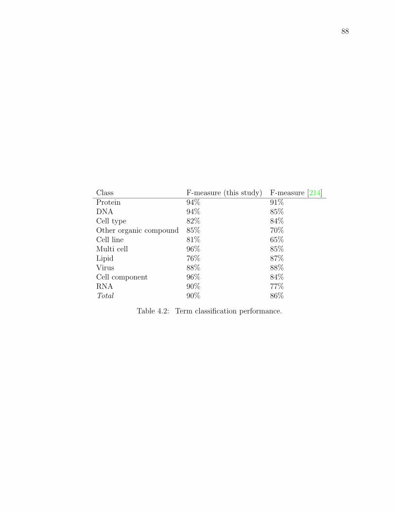
88
Class F-measure (this study) F-measure [214]Protein 94% 91%DNA 94% 85%Cell type 82% 84%Other organic compound 85% 70%Cell line 81% 65%Multi cell 96% 85%Lipid 76% 87%Virus 88% 88%Cell component 96% 84%RNA 90% 77%Total 90% 86%
Table 4.2: Term classification performance.

89
Chapter 5
Six senses: the bleak sensory
landscape of biomedical texts
It is beyond our power to fathom,Which way the word we utter resonates.Fedor Tyitchev
We analyzed the frequencies of use of sensory words (describing touch, smell, sight,
taste, and sound) and time-related terms in a very large collection of biomedical texts.
We then compared the results with similar analyses of a collection of news articles, a
large encyclopedia, and a body of literary prose and poetry. We found that, unlike
literary compositions and newswire articles, biomedical texts are extremely
sensory-poor, but rich in overall vocabulary. It is likely that the sensory-deprived
writing style that dominates the biomedical literature impedes text comprehension and
numbs the reader’s senses.
When we read technical or literary prose, chains of words flowing through our minds
invoke sensory responses that can be surprising (unexpected) even for the writer.
Even a very technical text typically affects the reader on multiple levels, in addition
to transmitting the author-intended content.

90
Prose can profoundly alter the physiological and emotional states of an unsuspecting
reader. The semantic priming test in modern psychology exploits this phenomenon.
For example, people start feeling and behaving as if they have suddenly grown older
after reading a scrambled sequence of words enriched with aging-related connotations
[215]. The priming effect is largely independent of our conscious understanding of a
text: autistic children whose text comprehension is mildly impaired respond to
semantic priming similarly to non-autistic kids [216]. Furthermore, our emotional
response to a sequence of words depends on our genetic background: for example,
children of parents with bipolar disorder react much more vividly to words that have
undertones of a social threat than do children in a control group [217]. Semantic
priming can profoundly affect the model of the outside world reported by our senses:
merely naming an odor (“cheddar cheese” vs. “body odor”) can determine our
perception of the odor as pleasant or nauseating [218].
The selection of words in a composition also reveals deep personality traits of its
author to the reader. For example, a person’s color preferences and idiosyncrasies
provide information relevant to her psychological evaluation [219]. Schizophrenia
patients—who are especially susceptible to semantic priming—have a characteristic
utterance pattern: the patients’ own words generate diverse secondary associations in
their minds. These self-inflicted associations surface in the patients’ utterances and
disturb the clarity of their messages [220].
Computational analysis of scientific language typically serves as the groundwork for
engineering text-mining tools [221, 222]. This analysis also provides us with a unique
glimpse into the “collective unconsciousness” of a scientific community. In this study
we compare the frequencies of sensory terms, such as those related to the perception
of color, smell, taste, touch, sound, and time, across multiple large corpora. We use
this comparison to infer a “collective sensory landscape” of the biomedical literature
and the hypothetical priming that biomedical texts exert on their readers.

91
We analyzed a large collection of scientific texts (Journals, including almost 250,000
full-text articles) representing 78 biomedical journals. We compared the properties of
biomedical texts with those of news reports (Reuters), the open-access encyclopedia
Wikipedia (Wiki), and complete collections of the compositions of Edgar Allan Poe
(Poe), William Shakespeare (Shakespeare), and Walt Whitman (Whitman). We
grouped these corpora into those that are collective (Journals, Reuters, and Wiki)
and those that are individual (Poe, Shakespeare, and Whitman).
When discussing time (Figure 5.1 A), all six corpora most frequently mention days
and years. In individual corpora, days predominate over all other time terms,
followed by hours and years. In collective corpora, years are most often mentioned,
followed by days and seconds. While individual corpora remain exclusively within the
second-to-century range, collective corpora reach into picoseconds on the short-term
side, and into millennia (and even millions of years, not shown) on the long-term side
of the range of time-scales. Within individual corpora, Whitman is the most
concerned with centuries, and Shakespeare the least. Reuters is almost twice as
time-obsessed as Whitman; all the other corpora are several-fold poorer in
time-conscious words (see Figure 5.1 E). Biomedical texts are among the poorest in
time-related terms, although Wiki and Shakespeare are even poorer.
When we consider words related to the five basic human senses (Figures 5.1 B and G),
sight-related terms are most frequent in all six corpora (Figure 5.1 B). The collective
prose is significantly more visual than the individual, but the trend is reversed for
taste, smell, touch, and sound-related terms. Among the individual corpora
Shakespeare is the least visual, but the richest in taste, smell, and touch-related
terms, when sensory word frequencies are normalized to sum to 1 within each corpus.
However, if we look at the absolute frequencies of sensory terms, the differences
between corpora are staggering (Figure 5.1 G): Whitman overall is the richest in
sensory terms, closely followed by Reuters. Poe, the next in ranking, reaches barely

92
half the frequency of sensory-related terms found in Reuters and Whitman. Compared
to Whitman and Reuters, sensory terms are nearly absent from Journals, Shakespeare,
and Wiki, with Wiki being the most sensory deprived. The balance between different
sensory terms (combined with the overall dictionary size) is visually highlighted in
Figure 5.1 D: individual corpora have, understandably, more limited vocabularies and
are significantly richer in non-visual sensory terms, but poorer in visual sensory terms,
than collective corpora. (Note that these differences in vocabulary richness, as well as
all other properties in Figure 5.1 D, are logarithmic rather than linear in scale.)
To highlight the similarities and dissimilarities in the frequencies of the numerous
sensory terms among the six corpora, we used a multidimensional scaling technique
[223] (see Figures 5.1 F and H). Multidimensional scaling at its heart is a task of
reconstructing a geographic map from a set of known distances between cities: in our
case, we are trying to arrange points corresponding to our six corpora on a plane so
that the resulting distances are as close as possible to the Euclidean distances
between corpus-specific vectors of frequencies of sensory terms. Both in the case of
the time-related (Figure 5.1 F) and the five-sense-related (Figure 5.1 H) terms, the
collective and individual corpora form two distinct groups. Shakespeare seems to be
an outlier in both cases, while Poe and Whitman are rather similar among the
individual corpora. Among the collective corpora, Journals and Wiki are the most
dissimilar, with Reuters occupying an intermediate position.
There are surprising and highly significant differences in the usage of color-related
terms among our six corpora—“our wits are so diversely colored” [224]. We grouped
color terms according to the taxonomy proposed by the anthropologists Berlin and
Kay [225, 226]. The Berlin-Kay taxonomy describes a hypothetical historical origin
and diversification of color terms summarized over 19 distinct cultures (see inset in
Figure 5.1 C). The authors suggest that color description is rather universal across
cultures, due to the universality of the anatomy and physiology of human vision.

93
Very briefly, according to their theory, as language develops in a typical culture,
description of color goes through several stages of complexity. The first stage involves
just two color terms, such as warm and cool, followed by the isolation of pure white
and pure black “colors”. At the later stages of color term differentiation, so-called
rellow color splits into red and yellow, while so-called grue splits into green and blue.
Journals and Reuters are nearly tied in the contest for the title of the visually
bleakest corpus. Reuters, the bleakest corpus (color-wise, but not in all sensory
terms), is significantly biased towards warm colors, while in Journals the frequencies
of various color-related terms are nearly uniform.
In all corpora but Poe, warm colors dominate over cold colors. In Poe, not only do
the cold colors prevail, but also black “color” dominates over all other colors at an
extremely high level of significance. Edgar Allan Poe’s prose and poetry is literally
dark. In Shakespeare’s writing the significantly dominant color is red-Shakespeare’s
prose is probably tinted by action in which blood is often spilled.
Unlike Poe and Shakespeare, Whitman produced texts with color term frequencies
nearly perfectly evenly distributed among the six major categories (white, black, red,
yellow, green, and blue; the frequency differences are not statistically significant).
This is particularly curious in light of the observation that Whitman’s writing overall
is twice as rich in color terms as that of Poe and Shakespeare and almost five times as
rich as biomedical prose (Journals).
What is the likely priming effect of biomedical texts on readers? Our conjecture
(which can be tested rigorously by experimental psychologists) is that the priming
effect is similar to the effect of a long journey through colorless flat terrain devoid of
prominent features—a numbing of the senses.
We suggest that apparently cognitively bleak biomedical texts can and should be
transformed into perceptually richer prose (we are not implying that it is an easy
task!). Why is this important? Because the mapping of abstract concepts to objects
94
with meaningful sensory properties serves as a stepping-stone to the solution of
complex problems. Consider the following quote from Richard Feynman.
I had a scheme, which I still use today when somebody is explainingsomething that I’m trying to understand: I keep making up examples. Forinstance, the mathematicians would come in with a terrific theorem, andthey’re all excited. As they’re telling me the conditions of the theorem, Iconstruct something which fits all the conditions. You know, you have aset (one ball)-disjoint (two balls). Then the ball turns colors, grow hairs,or whatever, in my head as they put more conditions on. Finally theystate the theorem, which is some dumb thing about the ball which isn’ttrue for my hairy green ball thing, so I say “False!”
If it’s true, they get all excited, and I let them go on for a while. Then Ipoint out my counterexample.
“Oh. We forgot to tell you that it’s Class 2 Hausdorff homomorphic.”
“Well, then,” I say, “It’s trivial! It’s trivial!” By that time I know whichway it goes, even though I don’t know what Hausdorff homomorphicmeans. [227]
(Credit for isolating this quote is due to Daniel Dennett [228].)
Our brain was shaped by a chain of evolutionary adaptations, each invoked by an
acute necessity to address a concrete survival problem posed by our changing
environment. Our neural system is therefore an eclectic ensemble of disparate pieces
of hardware, perfected for solving specialized problems-such as the detection of
potentially threatening bilateral vertical symmetry (a lurking predator) in the chaotic
environment, or prompt recognition of the faces of the numerous members of our own
tribe. To make more efficient use of our neural machinery, we need to translate
abstract problems into concrete sensory-grounded symbols that can be efficiently
processed by our brains. (This is like trying to do a general computation using
graphics-oriented hardware: to make the computation efficient, we have to translate
our task into spatial translations of three-dimensional primitives.)
When we read and compose sensory-deprived prose, we probably leave a large portion
of our nervous system uninvolved-different words and meanings are processed by
95
distinct brain areas [229]. We conjecture that a piece of sensory-poor prose does, on
average, a poorer job of engaging the reader’s imagination than a sensory-rich one,
although the former can be much more precise and concise than the latter. Within a
narrow scientific subfield, an expert would undoubtedly prefer to read a concise
technical text rather than a longer one replete with metaphors and analogies.
However, the situation is different for a scientist trying to read a paper from a
neighboring subfield: a dry technical description may require a prohibitive amount of
a non-expert’s time to read and grasp. It is in the writer’s best interest to ensure that
her work is as widely accessible as possible.
We believe that scientific prose should be enriched with sensory words (provided that
they clarify the meaning rather than obscure it), in much the same way as a good
statistical data visualization involves the mapping of abstract data into colors and
three-dimensional shapes, thus aiding the discovery of patterns.
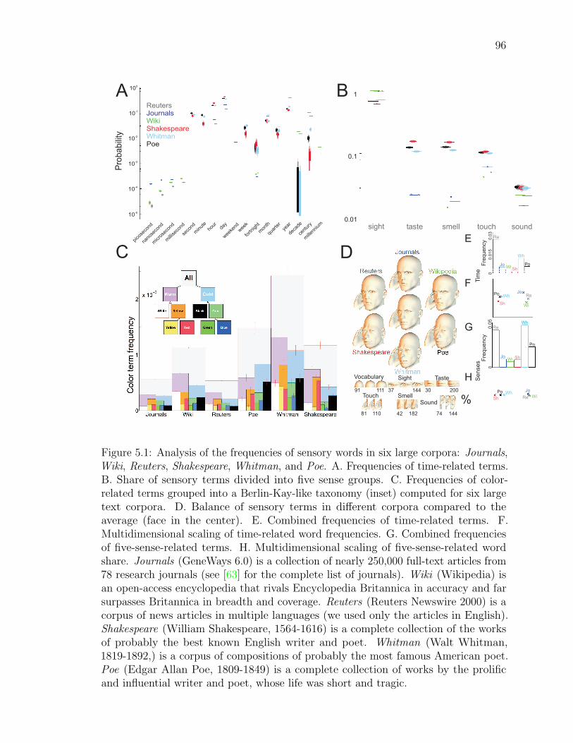
96
C
Vocabulary Sight Taste
Touch SmellSound
91 111 37 144 30 200
81 110 42 182 74 144
%
pico
seco
nd
nano
seco
nd
micro
seco
nd
milli
seco
nd
seco
nd
min
ute
hour
day
wee
kend
wee
k
fortn
ight
mon
th
quar
ter
deca
deye
ar
cent
ury
mille
nniu
m
10-5
10-4
10-3
10-2
10-1
100
Pro
babili
ty
ReutersJournalsWikiShakespeareWhitmanPoe
0.0
15
0
Fre
qu
en
cy
taste soundsmell touch
0.1
0.01sight
Fre
qu
en
cy
0.0
50
1BA
D
0.0
3
E
Senses
Tim
e
Wh
Wh
Wh
Wh
Wh
Sh
Sh
Sh
Sh
Wi
Wi
Wi
Wi
Jo
Jo
Jo
Jo
Re
Re
Re
Re
Po
Po
Po
Po
F
G
H
Figure 5.1: Analysis of the frequencies of sensory words in six large corpora: Journals,Wiki, Reuters, Shakespeare, Whitman, and Poe. A. Frequencies of time-related terms.B. Share of sensory terms divided into five sense groups. C. Frequencies of color-related terms grouped into a Berlin-Kay-like taxonomy (inset) computed for six largetext corpora. D. Balance of sensory terms in different corpora compared to theaverage (face in the center). E. Combined frequencies of time-related terms. F.Multidimensional scaling of time-related word frequencies. G. Combined frequenciesof five-sense-related terms. H. Multidimensional scaling of five-sense-related wordshare. Journals (GeneWays 6.0) is a collection of nearly 250,000 full-text articles from78 research journals (see [63] for the complete list of journals). Wiki (Wikipedia) isan open-access encyclopedia that rivals Encyclopedia Britannica in accuracy and farsurpasses Britannica in breadth and coverage. Reuters (Reuters Newswire 2000) is acorpus of news articles in multiple languages (we used only the articles in English).Shakespeare (William Shakespeare, 1564-1616) is a complete collection of the worksof probably the best known English writer and poet. Whitman (Walt Whitman,1819-1892,) is a corpus of compositions of probably the most famous American poet.Poe (Edgar Allan Poe, 1809-1849) is a complete collection of works by the prolificand influential writer and poet, whose life was short and tragic.
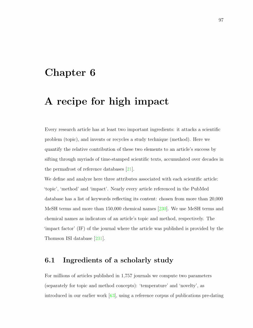
97
Chapter 6
A recipe for high impact
Every research article has at least two important ingredients: it attacks a scientific
problem (topic), and invents or recycles a study technique (method). Here we
quantify the relative contribution of these two elements to an article’s success by
sifting through myriads of time-stamped scientific texts, accumulated over decades in
the permafrost of reference databases [21].
We define and analyze here three attributes associated with each scientific article:
‘topic’, ‘method’ and ‘impact’. Nearly every article referenced in the PubMed
database has a list of keywords reflecting its content: chosen from more than 20,000
MeSH terms and more than 150,000 chemical names [230]. We use MeSH terms and
chemical names as indicators of an article’s topic and method, respectively. The
‘impact factor’ (IF) of the journal where the article was published is provided by the
Thomson ISI database [231].
6.1 Ingredients of a scholarly study
For millions of articles published in 1,757 journals we compute two parameters
(separately for topic and method concepts): ‘temperature’ and ‘novelty’, as
introduced in our earlier work [63], using a reference corpus of publications pre-dating

98
each article (see Additional data file 1). When all journal-specific articles are
considered together, a high temperature of a journal indicates its tendency to publish
popular (hot) concepts. The novelty parameter can change between 0 and 1, and, as
the name implies, reflects the proportion of new (previously unpublished) concepts in
a group of texts.
We used a five-parameter linear regression model to assess contributions of topic- and
method-specific estimates of temperature and novelty to a journal’s IF (see
Additional data file 1). We observe that high IFs correlate strongly with hotter topics
and colder methods (see Figure 6.1 a,b). Disturbingly, both method and topic novelty
are unimportant for predicting IF. Despite a strong positive correlation between the
popularity of article’s topic and method—contributed by the bulk of the moderately
influential articles (see Figure 6.1 b, inset)—the highest-impact scientific research
emerges when very popular (important) topics are tackled with unpopular methods.
Our topic and method terms have very different frequency distributions—reflecting
the difference in their genesis. In the former case, it is a human expert who decides
that a new concept is sufficiently frequently used to merit its addition to the
controlled MeSH vocabulary. In the latter case, the list of new terms is not artificially
restricted; they are allowed to be very rare (see Figure 6.1 b). As a result, frequencies
of the chemical terms follow a classical Zipf’s distribution, while MeSH terms clearly
deviate from this distribution due to deficiency of the rare terms (see Figure 6.1 b).
6.2 Information flow through publication-type
niches
Figure 6.1 c,d illustrates the unique (statistically distinct) niches of distinct
publication types in the space of novelty and temperature. For methods (chemicals,
including drugs), information diffuses from novel-unpopular to known-popular
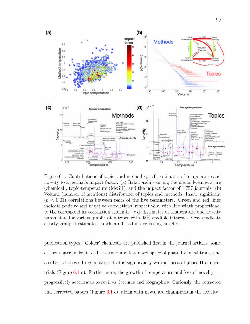
99
Figure 6.1: Contributions of topic- and method-specific estimates of temperature andnovelty to a journal’s impact factor. (a) Relationship among the method-temperature(chemical), topic-temperature (MeSH), and the impact factor of 1,757 journals. (b)Volume (number of mentions) distribution of topics and methods. Inset: significant(p < 0.01) correlations between pairs of the five parameters. Green and red linesindicate positive and negative correlations, respectively, with line width proportionalto the corresponding correlation strength. (c,d) Estimates of temperature and noveltyparameters for various publication types with 95% credible intervals. Ovals indicateclosely grouped estimates; labels are listed in decreasing novelty.
publication types. ‘Colder’ chemicals are published first in the journal articles; some
of them later make it to the warmer and less novel space of phase I clinical trials, and
a subset of these drugs makes it to the significantly warmer area of phase II clinical
trials (Figure 6.1 c). Furthermore, the growth of temperature and loss of novelty
progressively accelerates to reviews, lectures and biographies. Curiously, the retracted
and corrected papers (Figure 6.1 c), along with news, are champions in the novelty
100
competition—it looks almost as if the retracted articles are too novel to be correct.
For topics, we observe a similar—albeit less intuitive—picture (Figure 6.1 d), where
retracted articles again have the highest novelty. The clinical trial story shows a new
twist here: most clinical trials take years; they persist long enough for their initially
hot topics (at the stage of a research article and phase I clinical trial) to cool down
before reaching phase II and III trials (Figure 6.1 d)—a consequence of the
time-dependence of temperature estimates that capture ephemeral fads within
biological disciplines.
Our analysis highlights the importance of choice of a research topic, and of putting
new work in the right context. A remarkable idea (method) presented to the world in
a wrong context (topic) has little chance of being noticed. A successful idea travels
through publication types much as energy flows through an ecosystem: it is typically
born novel and unpopular in research articles (plants), and diffuses eventually to
reviews, lectures, clinical trials, and bibliographies (top-hierarchy carnivores), where
it reaches the pinnacle of popularity.
6.3 Additional information
6.3.1 Data
We parsed 8,592,483 PubMed records, extracting from each the PubMed ID, journal
name, year of publication, publication type, chemical names, and MeSH terms. We
chose a time-span between 1985 and 2004 characterized by a steady growth of the
number of MeSH terms, chemical names, and articles (Figure 6.2). Our dataset for
this period covers 12,039 journals that mention a total of 22,371 unique MeSH terms
and 153,756 unique chemical names. There are 49 different publication types.

101
Figure 6.2: Number of articles, MeSH terms and chemical names mentioned in PubMedsince 1950.
6.3.2 Analysis
A list of terms (MeSH terms or chemical names) that accompanies most time-stamped
records in the PubMed database allows us to monitor how popularity of terms
changes in time. Given a time point t, we define N it as the number of terms that occur
in PubMed before t exactly i times. To characterize the probability of encountering
terms with the same level of popularity (number of instances in PubMed before the
same point of time), we introduce a popularity variable q that takes integer values
0, 1, 2, . . .; notation P (q | t, parameter values) represents the expected proportion of
terms with popularity q at time point t given our model and parameter values.
When we model stochastic generation of scientific texts, we assume that each
time-stamped text is allowed to contain terms with zero popularity (novel terms), and
102
that the expected frequency of such terms is β, a parameter that we call novelty :
p(q = 0 | Nt, α, β) = β, (6.1)
where Nt is a vector summarizing all popularity counts associated with time point t.
We further assume that the expected frequency of known (q > 0) terms is
p(q | Nt, α, β) = (1− β)N qt q
α∑∞n=1N
nt n
α, (6.2)
where α is another model parameter that we call temperature.
We use Equations 6.1 and 6.2 to compute the likelihood of any collection of term
mentions given parameter values, and, assuming an uninformative prior parameter
distribution, estimate the joint posterior distribution of α and β.
In our analysis, we first estimate the novelty and temperature separately for topic
(MeSH) and method (chemical) content of articles published in journals that
mentioned at least 1,000 MeSH terms, and at least 1,000 chemicals within the chosen
interval, and had a known impact factor. This left us with a set of 1,757 journals.
The journal’s impact factor was computed as an average of its IF values reported
between 1999 and 2004.
We use the following linear regression model with a stepwise regression analysis
framework to test for a five-way correlation among journal specific parameters ( α and
β are temperature and novelty, respectively) and the impact factor (IF ) of a journal,
IFi = Aαtopic,i +Bβtopic,i + Cαmethod,i +Dβmethod,i + E + error, (6.3)
where subscript i refers to the ith journal and A, B, C, D and E are parameters of
the linear regression model. We assume that the error term follows a normal
distribution. Our analysis shows that estimates of B and D are not significantly
different from zero. The estimate for A is significantly larger than zero (4.55, with
103
95% confidence interval [3, 6]) and estimate for C is significantly smaller than zero
(-9.8, with 95% confidence interval [-12.6, -7]).
We estimate model parameters and credible intervals for publication types using a
version of the Markov chain Monte Carlo approach (see Figure 6.1 c and 1d; we use
the maximum posterior probability estimator in each case). Parameter estimation for
topics is done for publication types that mentioned at least 1,000 MeSH terms (same
selection strategy applies to parameter estimation for methods). ‘Average
temperature’ and ‘average novelty’ refers to a weighted average of temperature and
novelty when all publication types are considered together.
To fit the topic and method volumes to a Zipf’s (Pareto) distribution we use the
maximum likelihood estimate of γ-parameter of Zipf’s distribution; our estimates of
γ-values for topic and method volumes are 1.153 and 1.528, respectively.

104
Chapter 7
How many scientific papers should
be retracted?
7.1 Analyzing retraction patterns
Published scholarly articles commonly contain imperfections: punctuation errors,
imprecise wording and occasionally more substantial flaws in scientific methodology,
such as mistakes in experimental design, execution errors and even misconduct [232].
These imperfections are similar to manufacturing defects in man-made machines:
most are not dangerous but a small minority have the potential to cause a disaster
[233, 234]. Retracting a published scientific article is the academic counterpart of
recalling a flawed industrial product [235].
However, not all articles that should be retracted are retracted. This is because the
quality of a scientific article depends, among other things, on the effort and time
invested in quality control. Mechanical micro-fractures in turbojet components are
detected more readily than those in sculptures, as airplane parts are typically
subjected to much more rigorous testing for mechanical integrity. Similarly, articles
published in more prominent scientific journals receive increased attention and a
105
concomitant increase in the level of scrutiny. This therefore raises the question of how
many articles would have to be retracted if the highest standards of screening were
universally applied to all journals.
PubMed provides us with a ‘paleontological’ record of articles published in 4,348
journals with a known impact factor (IF). Of the 9,398,715 articles published between
1950 and 2004, 596 were retracted. This wave of retraction hits high-impact journals
significantly harder than lower-impact journals (Figure 7.1 A), suggesting that
high-impact journals are either more prone to publishing flawed manuscripts or
scrutinized much more rigorously than low-impact journals.
Here, we introduce a four-parameter stochastic model of the publication process (Fig
7.1 C), which allows us to investigate both possibilities (see Supplementary
Information for full details). The model describes the two sides of the
publicationretraction process: the rigor of a journal in accepting a smaller fraction of
flawed manuscripts (quality parameters α and θ), and post-publication scrutiny on
the part of the scientific community (scrutiny parameters β and τ). We need four
parameters to account for the possibility of both IF-independent and IF-dependent
changes in quality and scrutiny (see Fig 7.1 C, top). For each journal we compute a
normalized impact r (a journal-specific IF divided by the maximum IF value in our
collection of journals), and use it to define the strength of IF-dependent quality
(ralpha) and IF-dependent scrutiny (rbeta).
This probabilistic description allows us to distinguish between the two scenarios
described above for the higher incidence of retractions in high-impact journals. For
all values of τ tested, we find that the posterior mode of the IF-dependent quality
parameter (α) is close to 0 (Figure 7.1 B), indicating a nearly uniform and
IF-independent rigor in pre-publication quality control. Conversely, the posterior
mode of the IF-dependent scrutiny parameter (β) is essentially 1 (Figure 7.1 B),
which translates into a linear dependence between the IF of the journal and the rigor
106
of post-publication scrutiny. Our data therefore suggest that high-impact journals are
similar to their lower-impact peers in pre-publication scrutiny, but are much more
meticulously tested after publication.
Our model also allows us to estimate the number of papers that should have been
retracted under all plausible explanations of reality permitted by the model (Figure
7.1 C). We estimate the number of articles published between 1950 and 2004 that
ought to be retracted to be more than 100,000 under the more pessimistic scenario
(τ = 0.1; red, Figure 7.1 C), and greater than 10,000 under the most optimistic
scenario (τ = 1; green, Figure 7.1 C). The gap between retractable and retracted
papers is much wider for the lower-impact journals (Figure 7.1 C). For example, for
Nature (1999 - 2004 average IF = 29.5), with τ = 1 (optimistic), we estimate that
4567 articles should have been retracted, whereas only 30 actually were retracted.
Science (IF = 26.7) and Biochemistry (IF = 4.1) have nearly identical numbers of
papers published, but the actual numbers of retracted papers for these two journals
are 45 and 5 respectively.
Our analysis indicates that although high-impact journals tend to have fewer
undetected flawed articles than their lower-impact peers, even the most vigilant
journals potentially host papers that should be retracted. However, the positive
relationship between visibility of research and post-publication scrutiny suggests that
the technical and sociological progress in information disseminationthe internet,
omnipresent electronic publishing and the open access initiativeinadvertently
improves the self-correction of science by making scientific publications more visible
and accessible.
107
7.2 Mathematical model to calculate the number
of articles that should have been retracted
We analyzed the PubMed database, looking for retracted articles published between
1950 and 2004 in 4,348 journals with known impact factors (IFs) over a number of
years. Here we compute each journal’s impact factor as an average of its IF values
reported for the years 1999 to 2004 by ISI Thomson, Inc. Note that for some journals,
ISI provides different IF values in the bar charts and text on their website; we have
used the values described in the text.
Let IFi be the impact factor of the ith journal, and IFmax be the highest impact
factor that we observe in our dataset (50.551). We define a normalized IF for the ith
journal, ri, as ri = IFi
IFmax. Let ai be the total number of articles published in the ith
journal and ψi be the number of retracted articles in the same journal. According to
our model outlined in Figure 7.1 C (inset), the probability of observing retraction of
ψi out of ai articles published in the ith journal, computed jointly for all N journals
in our dataset (i = 1, . . . , n), is
p({ai, ψi, IFi} | Θ) =
∑i ai
a1 . . . an
∏i
p(IFi)ai
∏i
ai
ψi
[(1− θrαi ) τ rβi ]ψi [1− (1− θrαi ) τ rβi ]
(ai−ψi)
.
(7.1)
In this expression p(IFi) is the probability of sampling an article that is published in
the ith journal (with impact factor IFi). Note that the multinomial probability of
sampling the whole observed article set,
∑i ai
a1 . . . an
∏ni=1 p(IFi)
ai , and the
binomial coefficient,
ai
ψi
, do not depend on the values of our model parameters
and, therefore, they can be omitted in the maximum likelihood and MCMC
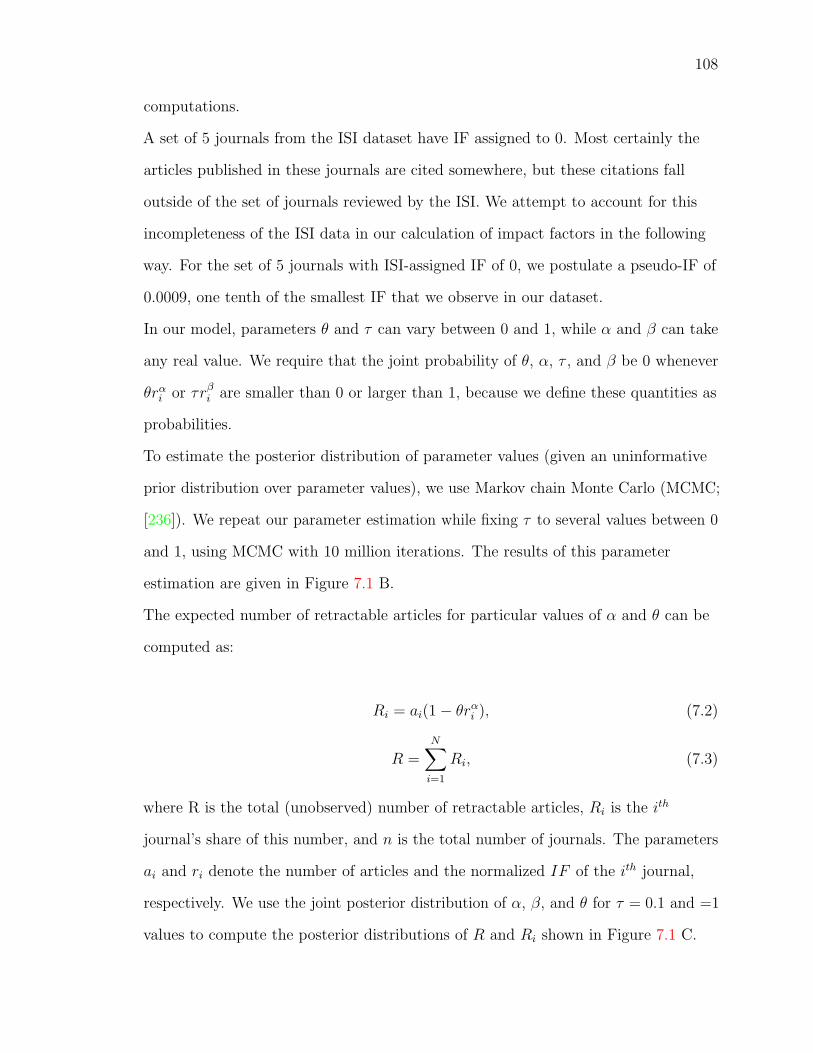
108
computations.
A set of 5 journals from the ISI dataset have IF assigned to 0. Most certainly the
articles published in these journals are cited somewhere, but these citations fall
outside of the set of journals reviewed by the ISI. We attempt to account for this
incompleteness of the ISI data in our calculation of impact factors in the following
way. For the set of 5 journals with ISI-assigned IF of 0, we postulate a pseudo-IF of
0.0009, one tenth of the smallest IF that we observe in our dataset.
In our model, parameters θ and τ can vary between 0 and 1, while α and β can take
any real value. We require that the joint probability of θ, α, τ , and β be 0 whenever
θrαi or τrβi are smaller than 0 or larger than 1, because we define these quantities as
probabilities.
To estimate the posterior distribution of parameter values (given an uninformative
prior distribution over parameter values), we use Markov chain Monte Carlo (MCMC;
[236]). We repeat our parameter estimation while fixing τ to several values between 0
and 1, using MCMC with 10 million iterations. The results of this parameter
estimation are given in Figure 7.1 B.
The expected number of retractable articles for particular values of α and θ can be
computed as:
Ri = ai(1− θrαi ), (7.2)
R =N∑i=1
Ri, (7.3)
where R is the total (unobserved) number of retractable articles, Ri is the ith
journal’s share of this number, and n is the total number of journals. The parameters
ai and ri denote the number of articles and the normalized IF of the ith journal,
respectively. We use the joint posterior distribution of α, β, and θ for τ = 0.1 and =1
values to compute the posterior distributions of R and Ri shown in Figure 7.1 C.

109
7.3 Retraction rates are on the rise
Like Shakespeare’s plays, scientific enterprise covers the whole spectrum of human
behavior ranging from genius, passion, and jealousy to mistakes and misconduct.
Although we are excited about advancements in science, our reaction to mistakes and
misconduct, and to the accompanying article retractions reflects the collapse of a
profound belief in the truth-seeking nature of the ideal scientist, who is devoid of
ordinary human flaws.
Recently, there have been a number of high-profile retractions in well regarded
journals which triggers a feeling that integrity of science is in decline. Are retraction
rates for scientific articles higher than in the past? Here, we demonstrate that this is
indeed the case.
We searched the Medline database to calculate the number of published articles and
the number of retracted articles since 1950. Our analysis indicates that more than 17
million articles have been recorded in Medline, and 871 of these have been retracted as
of 21 October 2007. Not surprisingly, the number of articles published in biomedical
sciences each year has been constantly increasing (Figure 1, black line). We divide
the number of retracted articles by the number of published articles each year to find
the percentage of articles retracted (Figure 7.2, red line). Figure 7.2 exhibits the first
cases of retractions in the 1970’s, which raised awareness of the issue and triggered
the establishment of the Office of Research Integrity (ORI). Interestingly, we find that
the rate of retracted articles has increased in time. The low retraction rates in the
first few decades of the studied period may stem from the possibility that Medline
had not flagged retracted articles at that time. However, even limiting our analysis to
the period between 1990 and 2006, we find a significant increase with r = 0.55
(p− value = 0.02). It must be noted that this figure underestimates the retraction
rates in recent years as there has not been sufficient time to identify the flawed
articles that were published in recent years (see the sharp decline in retraction rates
110
for 2007). Hence, if we were to analyze in future the retraction rate after the numbers
of retractions are saturated for the studied time period, we would expect to see an
even sharper increase in the rate of retracted articles. From these observations, we
conclude that retraction rates have been increasing.
This conclusion, of course, can have two interpretations, each with very different
implications for the state of science. The first interpretation implies that the ever
increasing competition in science and pressure to publish pushes scientists to produce
flawed manuscripts at a higher rate, which means scientific integrity is in decline. The
second interpretation is more positive, suggesting that flawed manuscripts are
identified more successfully, which means self-correction of science is improving.
In Chapter 7.1, we have shown that articles published in high-impact and highly
visible journals receive significantly greater scrutiny, and consequently there is a
higher chance for flawed articles to be identified in these journals. This study
suggested that self-correction in science will improve as continuing progress in the
dissemination of information (such as internet and electronic publishing) further
increases the visibility of research results. An increase of flawed manuscripts may still
be in effect, and this remains to be proved or disproved by further analysis. However,
with scientific knowledge becoming ever more visible each day, we may anticipate that
flawed manuscripts are more readily identified and self-correction in science is
improving.

111
Figure 7.1: Dataset, model and estimation of the number of flawed articles in scientificliterature. (A) Higher- and lower-impact factor (IF) journals have significantly morethan expected and less than expected retracted articles, respectively. Each sphererepresents the set of articles within the same IF range; the volume of the sphere isproportional to the set size and its color represents the middle-of-the-bin IF value.The expected number of retractions is calculated under the assumption that allretractions are uniformly distributed among articles and journals. The red lineindicates a hypothetical ideal correlation between the observed and the expectednumbers of retractions. (B) and (C) explain the four-parameter graphical modeldescribing our hypothetical stochastic publicationretraction process. (B) Estimatedposterior distribution of parameter values for several values of impact-independentscrutiny. (C) Outline of the stochastic graphical model (top) and the posterior meanestimates of the number of articles that should be retracted (with 95% credibleinterval) plotted against different values of IF. Posterior distributions of estimatednumber of retractable articles: red- and green-colored distributions correspond toτ = 0.1 and τ = 1, respectively; horizontal black solid lines indicate the actual numberof retracted articles for individual IF bins and journals. The contour distributionsrepresent individual journals, whereas the solid distributions correspond to the wholePubMed corpus binned by the IF value.

112
Figure 7.2: Number of articles and the percentage of articles retracted since 1950 asrecorded in Medline.

113
Chapter 8
Future work and conclusions
8.1 Future work
The work reported in Chapters 1 and 2 could be applied effectively to a more
standardized training/testing corpus. The automatic curation was adapted to the
GeneWays system, in principle, no reason to believe that it would not work in other
training/testing sets, but it certainly would have a sounder grounding if it were
replicated with a third-party dataset. The Collado-Vives laboratory [237, 238]
already has done so using data from the RegulonDB database of transcriptional
regulation in Escherichia coli. Further applications for automatic curation would have
their niche specifically in text-mining applications of low performance (that is, those
confronting a difficult mining problem).
Chapters 3 and 4 are different insofar as there already is extensive literature on the
topic considered. Nonetheless, the innovations in the approach and features presented
in these chapters could be easily applied to other fields—biomedical and
non-biomedical alike (e.g., web mining). A natural application would be to use
commercial web search engine results instead of our own processed corpora. The
ultimate objective would still be to hit the limits of the semantic space, or, more

114
conservatively, to approach and surpass human performance.
Chapter 5 introduced a new way to analyze the biomedical literature: its sensorial
impact over the reader. It is not hard to envision other measures of the impact that
the biomedical literature may have on its readers, such as emotional response,
engagement, and communicativeness. These measures could point to the impact and
consequences of the reading experience on the scientist. Chapter 6 represents another
journey to uncharted territory: finding ways for scientists to improve the impact of
their work. This study was limited to analysis of two parameters but models with
more parameters could be designed to capture more nuanced trends.
Chapter 7 is unique because it describes the first study designed to explore the
retraction phenomenon from an analytical point of view. Previous work was based on
empirical exploration and description of retracted articles. We believe that only
analytical approaches can answer questions like how retraction rates will change in
the future and how ingrained misconduct is in the scientific world. For example, is
retraction a mere phenomenon of bad apples or a systemic behavior contained only by
the watchdogs in place? Are the watchdogs effective? Another example is the analysis
of the retraction cycle, from submission to peer-review to publication to discovery to
retraction. Are there any hints that would allow us to be suspicious of a publication?
These and other questions are hot issue still open for analysis.
8.2 Conclusion
Text mining of the biomedical literature remains an open avenue for innovation both
in areas that seem mature and in areas that have yet to be thought of. The flexibility
of analyzing written language with more powerful resources and larger, better
repositories can only increase the quality of future work in this field.

115
8.3 Papers that resulted from the work in this
thesis
1. Rodriguez-Esteban R, Rzhetsky A. Biomedical term recognition and
classification using search engines. (in preparation)
2. Cokol M, Ozbay F, Rodriguez-Esteban R. Retraction rates are on the rise.
EMBO Rep. (in press)
3. Rodriguez-Esteban R, Rzhetsky A. Six senses: the bleak sensory landscape of
biomedical texts. EMBO Rep. (in press)
4. Cokol M, Rodriguez-Esteban R, Rzhetsky A. A recipe for high impact. Genome
Biol. 2007 May 10;8(5):406
5. Cokol M, Iossifov I, Rodriguez-Esteban R, Rzhetsky A. How many scientific
papers should be retracted? EMBO Rep. 2007 May;8(5):422-3.
6. Rodriguez-Esteban R, Iossifov I, Rzhetsky A. Imitating manual curation of
text-mined facts in biomedicine. PLoS Comput Biol. 2006 Sep 8;2(9)

Chapter 9
Bibliography
[1] Zanasi A. , ed.Text mining and its applications to intelligence, CRM and knowledge
management. Advances in Management InformationSouthampton, UK: WIT Press 2005.
[2] Kostoff R N. Science and Technology Text Mining: Pervasive Research Thrusts in the Former
Soviet Union (FSU) technical rept.Office of Naval Research 1995.
[3] Merkl D, Min Tjoa A. Data Mining in Large Free Text Document Archives in CODAS:269-276
1996.
[4] Feldman R, Dagan I. Knowledge Discovery in Textual Databases (KDT) in First International
Conference on Knowledge Discovery, KDD-95.(Montreal, Canada)AAAI Press 1995.
[5] Feldman R, Dagan I, Kloesgen W. Efficient Algorithms for Mining and Manipulating
Associations in Texts in EMCSR96(Vienna, Austria):949-954 1996.
[6] Feldman R, Hirsh H. Mining associations in text in the presence of background knowledge in
2nd International Conference on Knowledge Discovery and Data Mining (KDD-96):343-6 1996.
[7] Hearst M A. Untangling text data mining in ACL’99: the 37th Annual Meeting of the
Association for Computational Linguistics. 1999.
[8] Swanson D R. Undiscovered public knowledge. Libr Q. 1986;56:103-118.
[9] Bekhuis T. Conceptual biology, hypothesis discovery, and text mining: Swanson’s legacy
Biomed Digit Libr. 2006;3.
[10] Ananiadou S, McNaught J. , eds.Text mining for biology and biomedicine. Norwood, MA:
Artech House 2006.
116

117
[11] Natarajan J, Berrar D, Hack CJ., Dubitzky W. Knowledge discovery in biology and
biotechnology texts: a review of techniques, evaluation strategies, and applications Crit Rev
Biotechnol. 2005;25:31-52.
[12] Rajman M, Besancon R. Text Mining: Natural Language techniques and Text Mining
applications in 7th IFIP 2.6 Working Conference on Database Semantics (DS-7)IFIP
Proceedings(Leysin, Switzerland) 1997.
[13] Franke J, Nakhaeizadeh G, Renz I. , eds.Text Mining: Theoretical Aspects and Applications.
Advances in Soft ComputingHeidelberg: Physica-Verlag 2003.
[14] Weiss S, Indurkhya N, Zhang T, Damerau F. Text Mining. Predictive methods for analyzing
unstructured information. Science+Business MediaSpringer 2005.
[15] Feldman R, Sanger J. The text mining handbook: advanced approaches in analyzing
unstructured data. Cambridge University Press 2007.
[16] Kao A, Poteet S. , eds.Natural language processing and text mining. London: Springer-Verlag
2007.
[17] Fielden N. History of Information Retrieval Systems and Increase of Information Over Time in
Biennial California Academic And Research Librarians (CARL) Conference(Asilomar,
Monterey) 2002.
[18] Lyman P, Varian H R. How Much Information 2003. Retrieved from
http://www.sims.berkeley.edu/how-much-info-2003 on 9/2007.
[19] Lyman P, Varian H R. How Much Storage is Enough? ACM Queue. 2003;1.
[20] Weinstein J N. Integromic analysis of the NCI-60 cancer cell lines Breast Dis. 2004;19:11-22.
[21] Entrez PubMed, http://www.ncbi.nlm.nih.gov/entrez
[22] Xenarios I, Rice D W, Salwinski L, Baron M K, Marcotte E M, Eisenberg D. DIP: the
database of interacting proteins Nucleic Acids Res. 2000;28:289-91.
[23] Stark C, Breitkreutz B J, Reguly T, Boucher L, Breitkreutz A, Tyers M. BioGRID: a general
repository for interaction datasets Nucleic Acids Res. 2006;34:D535-9.
[24] Barrett T, Edgar R. Mining microarray data at NCBI’s Gene Expression Omnibus (GEO) in
Gene Mapping, Discovery, And Expression: Methods And Protocols (Bina Minou. ,
ed.):175-90Humana Press 2006.

118
[25] Hettne K M, Mos M, Bruijn AG., et al. Applied information retrieval and multidisciplinary
research: new mechanistic hypotheses in complex regional pain syndrome J Biomed Discov
Collab. 2007;2:2.
[26] Rebholz-Schuhman D, Cameron G, Clark D, et al. SYMBIOmatics: synergies in Medical
Informatics and Bioinformatics–exploring current scientific literature for emerging topics BMC
Bioinformatics. 2007;8 Suppl 1:S18.
[27] Takahashi Y, Miyaki K, Nakayama T. Analysis of news of the Japanese asbestos panic: a
supposedly resolved issue that turned out to be a time bomb J Public Health (Oxf).
2007;29:62-9.
[28] Cerrito P. Inside text mining. Text mining provides a powerful diagnosis of hospital quality
rankings Health Manag Technol. 2004;25:28-3.
[29] Ananiadou S, Kell D B, Tsujii J. Text mining and its potential applications in systems biology
Trends Biotechnol. 2006;24:571-9.
[30] Roberts P M. Mining literature for systems biology Brief Bioinform. 2006;7:399-406.
[31] Hoffmann R, Krallinger M, Andres E, Tamames J, Blaschke C, Valencia A. Text mining for
metabolic pathways, signaling cascades, and protein networks Sci STKE. 2005:pe21.
[32] Marcotte E M, Xenarios I, Eisenberg D. Mining literature for protein-protein interactions
Bioinformatics. 2001;17:359-63.
[33] Zanzoni A, Montecchi-Palazzi L, Quondam M, Ausiello G, Helmer-Citterich M, Cesareni G.
MINT: a Molecular INTeraction database FEBS Lett. 2002;513:135-40.
[34] Donaldson I, Martin J, Bruijn B, et al. PreBIND and Textomy–mining the biomedical
literature for protein-protein interactions using a support vector machine BMC Bioinformatics.
2003;4:11.
[35] Rzhetsky A, Iossifov I, Koike T, et al. GeneWays: a system for extracting, analyzing,
visualizing, and integrating molecular pathway data J Biomed Inform. 2004;37:43-53.
[36] Sekimizu T, Park H S, Tsujii J. Identifying the Interaction between Genes and Gene Products
Based on Frequently Seen Verbs in Medline Abstracts Genome Inform Ser Workshop Genome
Inform. 1998;9:62-71.
[37] Rindflesch T C, Hunter L, Aronson A R. Mining molecular binding terminology from
biomedical text Proc AMIA Symp. 1999:127-31.

119
[38] Stapley B J, Benoit G. Biobibliometrics: information retrieval and visualization from
co-occurrences of gene names in Medline abstracts Pac Symp Biocomput. 2000:529-40.
[39] Jenssen T K, Laegreid A, Komorowski J, Hovig E. A literature network of human genes for
high-throughput analysis of gene expression Nat Genet. 2001;28:21-8.
[40] Sanchez-Graillet O, Poesio M. Negation of protein-protein interactions: analysis and
extraction Bioinformatics. 2007;23:i424-32.
[41] Pustejovsky J, Castano J, Zhang J, Kotecki M, Cochran B. Robust relational parsing over
biomedical literature: extracting inhibit relations Pac Symp Biocomput. 2002:362-73.
[42] Blaschke C, Andrade M A, Ouzounis C, Valencia A. Automatic extraction of biological
information from scientific text: protein-protein interactions Proc Int Conf Intell Syst Mol
Biol. 1999:60-7.
[43] Thomas J, Milward D, Ouzounis C, Pulman S, Carroll M. Automatic extraction of protein
interactions from scientific abstracts Pac Symp Biocomput. 2000:541-52.
[44] Proux D, Rechenmann F, Julliard L. A pragmatic information extraction strategy for
gathering data on genetic interactions Proc Int Conf Intell Syst Mol Biol. 2000;8:279-85.
[45] Humphreys K, Demetriou G, Gaizauskas R. Two applications of information extraction to
biological science journal articles: enzyme interactions and protein structures Pac Symp
Biocomput. 2000:505-16.
[46] Rindflesch T C, Tanabe L, Weinstein J N, Hunter L. EDGAR: extraction of drugs, genes and
relations from the biomedical literature Pac Symp Biocomput. 2000:517-28.
[47] Blaschke C, Valencia A. The potential use of SUISEKI as a protein interaction discovery tool
Genome Inform. 2001;12:123-34.
[48] Blaschke C, Valencia A. The Frame-Based Module of the SUISEKI Information Extraction
System IEEE Intelligent Systems. 2002;17:14-20.
[49] Park J C, Kim H S, Kim J J. Bidirectional incremental parsing for automatic pathway
identification with combinatory categorial grammar Pac Symp Biocomput. 2001:396-407.
[50] Yakushiji A, Tateisi Y, Miyao Y, Tsujii J. Event extraction from biomedical papers using a
full parser Pac Symp Biocomput. 2001:408-19.

120
[51] Friedman C, Kra P, Yu H, Krauthammer M, Rzhetsky A. GENIES: a natural-language
processing system for the extraction of molecular pathways from journal articles
Bioinformatics. 2001;17 Suppl 1:S74-82.
[52] Friedman C, Alderson P O, Austin J H, Cimino J J, Johnson S B. A general natural-language
text processor for clinical radiology J Am Med Inform Assoc. 1994;1:161–174.
[53] Friedman C, Kra P, Rzhetsky A. Two biomedical sublanguages: a description based on the
theories of Zellig Harris J Biomed Inform. 2002;35:222–235.
[54] Altschul S F, Gish W, Miller W, Myers E W, Lipman D J. Basic local alignment search tool J
Mol Biol. 1990;215:403-10.
[55] Krauthammer M, Rzhetsky A, Morozov P, Friedman C. Using BLAST for identifying gene
and protein names in journal articles Gene. 2000;259:245-52.
[56] Hoffmann R, Valencia A. A gene network for navigating the literature Nat Genet. 2004;36:664.
[57] Fernandez J M, Hoffmann R, Valencia A. iHOP web services Nucleic Acids Res.
2007;35:W21-6.
[58] Koike A, Niwa Y, Takagi T. Automatic extraction of gene/protein biological functions from
biomedical text Bioinformatics. 2005;21:1227-36.
[59] Hatzivassiloglou V, Duboue P A, Rzhetsky A. Disambiguating proteins, genes, and RNA in
text: a machine learning approach Bioinformatics. 2001;17 Suppl 1:S97-106.
[60] Rzhetsky A, Koike T, Kalachikov S, et al. A knowledge model for analysis and simulation of
regulatory networks Bioinformatics. 2000;16:1120-8.
[61] Krauthammer M, Kaufmann C A, Gilliam T C, A Rzhetsky. Molecular triangulation: bridging
linkage and molecular-network information for identifying candidate genes in Alzheimer’s
disease Proc Natl Acad Sci U S A. 2004;101:15148-53.
[62] Iossifov I, Krauthammer M, Friedman C, et al. Probabilistic inference of molecular networks
from noisy data sources Bioinformatics. 2004;20:1205-13.
[63] Cokol M, Iossifov I, Weinreb C, Rzhetsky A. Emergent behavior of growing knowledge about
molecular interactions Nat Biotechnol. 2005;23:1243–1247.
[64] Rzhetsky A, Zheng T, Weinreb C. Self-correcting maps of molecular pathways PLoS ONE.
2006;1:e61.

121
[65] Rzhetsky A, Iossifov I, Loh J M, White K P. Microparadigms: chains of collective reasoning in
publications about molecular interactions Proc Natl Acad Sci U S A. 2006;103:4940-5.
[66] Krauthammer M, Kra P, Iossifov I, et al. Of truth and pathways: chasing bits of information
through myriads of articles Bioinformatics. 2002;18 Suppl. 1:S249–S257.
[67] Friedman C, Hripcsak G. Evaluating natural language processors in the clinical domain
Methods Inf Med. 1998;37:334-44.
[68] Ono T, Hishigaki H, Tanigami A, Takagi T. Automated extraction of information on
protein-protein interactions from the biological literature Bioinformatics. 2001;17:155-61.
[69] BioCreAtIvE - Critical Assessment for Information Extraction in Biology
[70] CAPRI: Critical Assessment of PRediction of Interactions
[71] Daraselia N, Yuryev A, Egorov S, Novichkova S, Nikitin A, Mazo I. Extracting human protein
interactions from MEDLINE using a full-sentence parser Bioinformatics. 2004;20:604-11.
[72] Chen H, Sharp B M. Content-rich biological network constructed by mining PubMed abstracts
BMC Bioinformatics. 2004;5:147.
[73] Hakenberg J, Plake C, Leser U. Optimizing Syntax Patterns for Discovering Protein-Protein
Interactions in ACM Symposium on Applied Computing (SAC), Bioinformatics Track.
2005:195–201 2005.
[74] Century King James Bible Publishers . The Holy Bible : 21st Century King James Version :
containing the Old Testament and the New Testament. Gary, SD: 21st Century King James
Bible Publishers 1994.
[75] Carletta J. Assessing Agreement on Classification Tasks: The Kappa Statistic Computational
Linguistics. 1996;22:249–254.
[76] Ruan W, Pang P, Rao Y. The SH2/SH3 adaptor protein dock interacts with the Ste20-like
kinase misshapen in controlling growth cone motility Neuron. 1999;24:595–605.
[77] Chan Y M, Jan Y N. Presenilins, processing of beta-amyloid precursor protein, and notch
signaling Neuron. 1999;23:201–204.
[78] Niethammer M, Smith D S, Ayala R, et al. NUDEL is a novel Cdk5 substrate that associates
with LIS1 and cytoplasmic dynein Neuron. 2000;28:697–711.
122
[79] Alloway P G, Howard L, Dolph P J. The formation of stable rhodopsin-arrestin complexes
induces apoptosis and photoreceptor cell degeneration Neuron. 2000;28:129–138.
[80] Tanaka H, Shan W, Phillips G R, et al. Molecular modification of N-cadherin in response to
synaptic activity Neuron. 2000;25:93–107.
[81] Magga J M, Jarvis S E, Arnot M I, Zamponi G W, Braun J E. Cysteine string protein
regulates G protein modulation of N-type calcium channels Neuron. 2000;28:195–204.
[82] Gordon S E, Varnum M D, Zagotta W N. Direct interaction between amino- and
carboxyl-terminal domains of cyclic nucleotide-gated channels Neuron. 1997;19:431–441.
[83] Gad H, Ringstad N, Low P, et al. Fission and uncoating of synaptic clathrin-coated vesicles
are perturbed by disruption of interactions with the SH3 domain of endophilin Neuron.
2000;27:301–312.
[84] Van Vactor D, Flanagan J G. The middle and the end: slit brings guidance and branching
together in axon pathway selection Neuron. 1999;22:649–652.
[85] Benson D A, Karsch-Mizrachi I, Lipman D J, Ostell J, Wheeler D L. GenBank Nucleic Acids
Res. 2005;33:D34–38.
[86] Fisher R A. The use of multiple measurements in taxonomic problems Ann Eugenic.
1936;7:179–188.
[87] Jaynes E T. Information Theory and Statistical Mechanics Physical Review. 1957;106:620–630.
[88] Jaynes E T, Bretthorst G L. Probability theory : the logic of science. Cambridge, UK ; New
York, NY: Cambridge University Press 2003.
[89] Cover T M, Thomas J A. Elements of information theory. Hoboken, NJ.: J. Wiley2nd ed.
2005.
[90] Chauvin Y, Rumelhart D E. Backpropagation : theory, architectures, and applications.
Developments in connectionist theoryHillsdale, NJ.: Erlbaum 1995.
[91] Vapnik V N. The nature of statistical learning theory. Statistics, Computer Science,
PsychologyNew York: Springer 1995.
[92] Cristianini N, Shawe-Taylor J. An introduction to support vector machines : and other
kernel-based learning methods. Cambridge, New York: Cambridge University Press 2000.
[93] Smola A J. Advances in large margin classifiers. Cambridge, Mass.: MIT Press 2000.
123
[94] Joachims T. Making large-scale support vector machine learning practical in Advances in
Kernel Methods: Support Vector Machines (Scholkopf B., Burges C, Smola A. , eds.)MIT
Press, Cambridge, MA 1998.
[95] Ratnaparkhi A. A maximum entropy part-of-speech tagger in Empirical Methods in Natural
Language Processing(University of Pennsylvania, Philadelphia):491-497 1996.
[96] Hanley J A, McNeil B J. The meaning and use of the area under a receiver operating
characteristic (ROC) curve Radiology. 1982;143:29–36.
[97] Turing A M. Computing machinery and intelligence Mind. 1950;59:433–560.
[98] Church K W, Hanks P. Word association norms, mutual information, and lexicography in
Proceedings of the 27th annual meeting on Association for Computational
Linguistics(Morristown, NJ, USA):76–83Association for Computational Linguistics 1989.
[99] Shannon C E, Weaver W. The mathematical theory of communication. Urbana: University of
Illinois Press 1949.
[100] Neumann J. Probabilistic Logics and the Synthesis of Reliable Organisms from Unreliable
Components in Automata Studies (Shannon C E, McCarthy J. , eds.):43–98Princeton, NJ:
Princeton University Press 1956.
[101] Krauthammer M, Nenadic G. Term identification in the biomedical literature J Biomed
Inform. 2004;37:512-26.
[102] Kageura K, Umino B. Methods of Automatic Term Recognition -A Review- Terminology.
1996;3:259-289.
[103] Luhn H P. A statistical approach to mechanized encoding and searching of literary
information IBM Journal of Research and Development. 1957;2:159-165.
[104] Sager J C. A Practical Course in Terminology Processing. Amsterdam/Philadelphia:
Benjamins 1990.
[105] Sekine S. Named Entity: History and Future tech. rep. 2004.
[106] Grishman R, Sundheim B. Message Understanding Conference-6: a brief history in 16th
conference on Computational linguistics;1:466 - 471 1996.
[107] Chinchor N. Overview of MUC-7 in 7th Message Understanding Conference (MUC-7)(Fairfax,
Virginia) 1998.

124
[108] Merchant R, Okurowski M E, N Chinchor. The multilingual entity task (MET) overview in
Annual Meeting of the ACL(Vienna, Virginia):445-447 1996.
[109] Sparck-Jones K. Automatic term classification and information retrieval in IFIP
Congress:1290-1295 1968.
[110] Sparck-Jones K. Automatic keyword classification for information retrieval. London, UK:
Butterworths 1971.
[111] Sparck-Jones K. Collection Properties Influencing Automatic Term Classification Performance
Information Storage and Retrieval. 1973;9:499-513.
[112] Kilgarriff A. What is word sense disambiguation good for? in Natural Language Processing
Pacific Rim Symposium(Phuket, Thailand):209-214 1997.
[113] Stevenson M, Wilks Y. The interaction of knowledge sources in word sense disambiguation
Computational Linguistics. 2001;27:321-349.
[114] Agirre E, Martinez D. Knowledge Sources for Word Sense Disambiguation in Text, Speech and
DialogueLecture Notes in Computer ScienceSpringer Berlin / Heidelberg 2004.
[115] Collins M, Singer Y. Unsupervised models for named entity classification in EMNLP 1999.
[116] Black W, Vasilakopoulos A. Language independent named entity classification by modified
transformation-based learning and by decision tree induction in 6th conference on Natural
language learning;20:1-4 2002.
[117] Kim J, Kang I, Choi K. Unsupervised named entity classification models and their ensembles
in 19th international conference on Computational linguistics;1(Taipei, Taiwan):1-7 2002.
[118] Hahn U, Schnattinger K. Towards text knowledge engineering in Fifteenth national/tenth
conference on Artificial intelligence/Innovative applications of artificial intelligence(Madison,
Wisconsin, United States):524 - 531 1998.
[119] Alfonseca E, Manandhar S. Extending a Lexical Ontology by a Combination of Distributional
Semantics Signatures in 13th International Conference on Knowledge Engineering and
Knowledge Management. Ontologies and the Semantic Web:1-7 2002.
[120] Cimiano P, Volker J. Towards large-scale, open-domain and ontology-based named entity
classification in International Conference on Recent Advances in Natural Language Processing
(RANLP) (Angelova G, Bontcheva K, Mitkov R, Nicolov N. , eds.)(Borovets,
Bulgaria):166-172 2005.

125
[121] Fleischman M. Automated subcategorization of named entities ACL Student Workshop. 2001.
[122] Fleischman M, Hovy E. Fine grained classification of named entities. in 19th international
conference on Computational linguistics;1(Taipei, Taiwan):1-7 2002.
[123] Lee C, Hwang Y, Oh H, et al. Fine-Grained Named Entity Recognition Using Conditional
Random Fields for Question Answering in Information Retrieval Technology;4182/2006 of
Lecture Notes in Computer Science:581-587Springer Berlin / Heidelberg 2006.
[124] Fukuda K, Tamura A, Tsunoda T, Takagi T. Toward information extraction: identifying
protein names from biological papers Pac Symp Biocomput. 1998:707-18.
[125] Ananiadou S. Automatic recognition of medical terminology (immunology) in Medinfo;8 Pt
1:3-7 1995.
[126] Tsai R T, Wu S H, Chou W C, et al. Various criteria in the evaluation of biomedical named
entity recognition BMC Bioinformatics. 2006;7:92.
[127] Collier N, Park H S, Ogata N, et al. The GENIA project: corpus-based knowledge acquisition
and information extraction from genome research papers in European Association for
Computational Linguistics 1999.
[128] Franzen K, Eriksson G, Olsson F, Asker L, Liden P, Coster J. Protein names and how to find
them Int J Med Inform. 2002;67:49-61.
[129] Kim J D, Ohta T, Tsuruoka Y, Tateisi Y, Collier N. Introduction to the Bio-Entity
Recognition Task at the Joint Workshop on Natural Language Processing in Biomedicine and
its Applications in Joint Workshop on Natural Language Processing in Biomedicine and its
Applications(Geneva, Switzerland) 2004.
[130] Hirschman L, Yeh A, Blaschke C, Valencia A. Overview of BioCreAtIvE: critical assessment of
information extraction for biology BMC Bioinformatics. 2005;6 Suppl 1:S1.
[131] Nobata C, Collier N, Tsujii J. Automatic Term Identification and Classification in Biology
Texts in Natural Language Pacific Rim Symposium 1999.
[132] Mukherjea S, Subramaniam L V, Chanda G, et al. Enhancing a biomedical information
extraction system with dictionary mining and context disambiguation IBM Journal of
Research and Development. 2004;48:693-702.
[133] Lee K J, Hwang Y S, Kim S, Rim H C. Biomedical named entity recognition using two-phase
model based on SVMs J Biomed Inform. 2004;37:436-47.

126
[134] Takeuchi K, Collier N. Bio-medical entity extraction using support vector machines Artif Intell
Med. 2005;33:125-37.
[135] Frantzi K, Ananiadou S, Tsujii J. Classifying Technical Terms in Redefining the Information
Chain New Ways and Voices (Smith J W T, Ardo A, Linde P. , eds.):144-155ICCC Press
1999.
[136] Nenadic G, Spasic I, Ananiadou S. Terminology-driven mining of biomedical literature
Bioinformatics. 2003;19:938-943.
[137] Lindberg C. The Unified Medical Language System (UMLS) of the National Library of
Medicine J Am Med Rec Assoc. 1990;61:40-2.
[138] Lovis C, Michel P A, Baud R, Scherrer J R. Word segmentation processing: a way to
exponentially extend medical dictionaries in Medinfo;8 Pt 1:28-32 1995.
[139] Cohen K B, Dolbey A E, Acquaah-Mensah G K, Hunter L. Contrast and variability in gene
names in ACL Workshop on Natural Language Processing in the Biomedical Domain:14-20
2002.
[140] Olsson F, Eriksson G, Franzen K, Asker L, Liden P. Notions of correctness when evaluating
protein name taggers in 19th international conference on computational linguistics:76571 2002.
[141] Mika S, Rost B. Protein names precisely peeled off free text Bioinformatics. 2004;20 Suppl
1:i241-7.
[142] Maclean K. Humour of gene names lost in translation to patients Nature. 2006;439:266.
[143] Collier N, Takeuchi K. Comparison of character-level and part of speech features for name
recognition in biomedical texts Journal of Biomedical Informatics. 2004;37:423-435.
[144] Torii M, Kamboj S, Vijay-Shanker K. An investigation of various information sources for
classifying biological names in ACL workshop on Natural language processing in
biomedicine(Sapporo, Japan):113-120 2003.
[145] Morgan A, Hirschman L, Yeh A, Colosimo M. Gene name extraction using FlyBase resources
in Annual Meeting of the ACL archive. Workshop on Natural language processing in
biomedicine;13(Sapporo, Japan):1 - 8 2003.
[146] Craven M, Kumlien J. Constructing Biological Knowledge Bases by Extracting Information
from Text Sources in Seventh International Conference on Intelligent Systems for Molecular
Biology:77-86 1999.
127
[147] Yamamoto K, Kudo T, Konagaya A, Matsumoto Y. Protein name tagging for biomedical
annotation in text in ACL 2003 workshop on natural language processing in biomedicine:65-72
2003.
[148] Chang J T, Schutze H, Altman R B. GAPSCORE: finding gene and protein names one word
at a time Bioinformatics. 2004;20:216-25.
[149] Hanisch D, Fluck J, Mevissen H T, Zimmer R. Playing biology’s name game: identifying
protein names in scientific text in Pac Symp Biocomput:403-14 2003.
[150] Narayanaswamy M, Ravikumar K E, Vijay-Shanker K. A biomedical named entity recognizer
in Pacific Symposium on Biocomputing;8:427-438 2003.
[151] Hou W-J, Chen H-H. Enhancing performance of protein name recognizers using collocation in
Annual Meeting of the ACL. Workshop on Natural language processing in
biomedicine;13(Sapporo, Japan):25-32 2003.
[152] Gaizauskas R, Demetriou G, Artymiuk P J, Willett P. Protein Structures and Information
Extraction from Biological Texts: The PASTA System Bioinformatics. 2003;19:135-43.
[153] Tanabe L, Wilbur W J. Tagging gene and protein names in biomedical text Bioinformatics.
2002;18:1124-32.
[154] Wilbur W J. Boosting naive Bayesian learning on a large subset of MEDLINE Proc AMIA
Symp. 2000:918-22.
[155] Stapley B J, Kelley L A, Sternberg M J. Predicting the sub-cellular location of proteins from
text using support vector machines Pac Symp Biocomput. 2002:374-85.
[156] Kazama J, Makino T, Ohta Y, Tsujii J. Tuning support vector machines for biomedical named
entity recognition in Annual Meeting of the ACL archive. ACL-02 workshop on Natural
language processing in the biomedical domain;3(Phildadelphia, Pennsylvania):1-8 2002.
[157] Mika S, Rost B. NLProt: extracting protein names and sequences from papers Nucleic Acids
Res. 2004;32:W634-7.
[158] Shi L, Campagne F. Building a protein name dictionary from full text: a machine learning
term extraction approach BMC Bioinformatics. 2005;6:88.
[159] Collier N, Nobata C, Tsujii J. Extracting the Names of Genes and Gene Products with a
Hidden Markov Model in COLING:201-07 2000.
128
[160] Zhou G, Zhang J, Su J, Shen D, Tan C. Recognizing names in biomedical texts: a machine
learning approach Bioinformatics. 2004;20:1178-90.
[161] Zhang J, Shen D, Zhou G, Su J, Tan C L. Enhancing HMM-based biomedical named entity
recognition by studying special phenomena J Biomed Inform. 2004;37:411-22.
[162] Finkel J, Dingare S, Manning C D, Nissim M, Alex B, Grover C. Exploring the boundaries:
gene and protein identification in biomedical text BMC Bioinformatics. 2005;6 Suppl 1:S5.
[163] McDonald R T, Winters R S, Mandel M, Jin Y, White P S, Pereira F. An entity tagger for
recognizing acquired genomic variations in cancer literature Bioinformatics. 2004;17:3249-51.
[164] Settles B. Biomedical named entity recognition using conditional random fields and novel
feature sets in Joint Workshop on Natural Language Processing in Biomedicine and its
Application:104-107 2004.
[165] Sun C, Guan Y, Wang X, Lin L. Rich features based Conditional Random Fields for biological
named entities recognition Computers in Biology and Medicine archive. 2007;37:1327-1333.
[166] Hou W J, Chen H H. Enhancing performance of protein and gene name recognizers with
filtering and integration strategies J Biomed Inform. 2004;37:448-60.
[167] Liu H, Lussier Y A, Friedman C. Disambiguating ambiguous biomedical terms in biomedical
narrative text: an unsupervised method J Biomed Inform. 2001;34:249-61.
[168] Liu H, Johnson S B, Friedman C. Automatic resolution of ambiguous terms based on machine
learning and conceptual relations in the UMLS J Am Med Inform Assoc. 2002;9:621-36.
[169] Liu H, Teller V, Friedman C. A multi-aspect comparison study of supervised word sense
disambiguation J Am Med Inform Assoc. 2004;11:320-31.
[170] Ruch P, Baud R, Geissbuhler A. Using lexical disambiguation and named-entity recognition to
improve spelling correction in the electronic patient record Artif Intell Med. 2003;29:169-84.
[171] Ginter F, Boberg J, Jarvinen J, Salakoski T. New Techniques for Disambiguation in Natural
Language and Their Application to Biological Text The Journal of Machine Learning
Research. 2004;5:605 - 621.
[172] Leroy G, Rindflesch T C. Effects of information and machine learning algorithms on word
sense disambiguation with small datasets Int J Med Inform. 2005;74:573-85.

129
[173] Xu H, Markatou M, Dimova R, Liu H, Friedman C. Machine learning and word sense
disambiguation in the biomedical domain: design and evaluation issues BMC Bioinformatics.
2006;7:334.
[174] Chen P, Al-Mubaid H. Context-based Term Disambiguation in Biomedical Literature in
FLAIRS(Orlando, Fla) 2006.
[175] Weeber M, Mork J G, Aronson A R. Developing a test collection for biomedical word sense
disambiguation Proc AMIA Symp. 2001:746-50.
[176] Schuemie M J, Kors J A, B Mons. Word sense disambiguation in the biomedical domain: an
overview J Comput Biol. 2005;12:554-65.
[177] Gale W A, Church K W, Yarowsky D. One sense per discourse in Human Language
Technology Conference. Workshop on Speech and Natural Language:233 - 237 1992.
[178] Krovetz R. More than one sense per discourse tech. rep.NEC Princeton NJ Labs 1998.
[179] Martinez D, Agirre E. One sense per collocation and genre/topic variations in Annual Meeting
of the ACL. Joint SIGDAT conference on Empirical methods in natural language processing
and very large corpora: held in conjunction with the 38th Annual Meeting of the Association
for Computational Linguistics;13:207-215 2000.
[180] Kilgarriff A. 95% replicability for manual word sense tagging in 9th Conference of the
European Chapter Association of Computational Linguistics:277-278 1999.
[181] Pustejovsky J, Castano J, Cochran B, Kotecki M, Morrell M. Automatic extraction of
acronym-meaning pairs from MEDLINE databases Medinfo. 2001;10(Pt 1):371-5.
[182] Chang J T, Schutze H, Altman R B. Creating an online dictionary of abbreviations from
MEDLINE J Am Med Inform Assoc. 2002;9:612-20.
[183] Schwartz A S, Hearst M A. A simple algorithm for identifying abbreviation definitions in
biomedical text Pac Symp Biocomput. 2003:451-62.
[184] Pakhomov S., Pedersen T, Chute C G. Abbreviation and acronym disambiguation in clinical
discourse in AMIA Annu Symp:589-93 2005.
[185] Okazaki N, Ananiadou S. Building an abbreviation dictionary using a term recognition
approach Bioinformatics. 2006;22:3089-95.
[186] Zhou W, Torvik V I, Smalheiser N R. ADAM: another database of abbreviations in
MEDLINE Bioinformatics. 2006;22:2813-8.
130
[187] Yu H, Kim W, Hatzivassiloglou V, Wilbur W J. Using MEDLINE as a knowledge source for
disambiguating abbreviations and acronyms in full-text biomedical journal articles J Biomed
Inform. 2007;40:150-9.
[188] Pyysalo S, Salakoski T, Aubin S, Nazarenko A. Lexical adaptation of link grammar to the
biomedical sublanguage: a comparative evaluation of three approaches BMC Bioinformatics.
2006;7 Suppl 3:S2.
[189] Cohen W W, Ravikumar P, Fienberg S E. A comparison of string distance metrics for
name-matching tasks in IJCAI-2003 Workshop on Information Integration on the Web 2003.
[190] Wellner Ben, Castano Jose, Pustejovsky James. Adaptive String Similarity Metrics for
Biomedical Reference Resolution in ACL-ISMB Workshop on Linking Biological Literature,
Ontologies and Databases: Mining Biological Semantics(Detroit):9–16Association for
Computational Linguistics 2005.
[191] Al-Mubaid H. Context-Based Technique for Biomedical Term Classification in IEEE Congress
on Evolutionary Computation(Vancouver, Canada):5726-5733 2006.
[192] Spasic I, Ananiadou S. Using automatically learnt verb selectional preferences for classification
of biomedical terms J Biomed Inform. 2004;37:483-97.
[193] McDonald D. Internal and external evidence in the identification and semantic categorization
of proper names in Corpus Processing for Lexical Acquisition (Boguraev B, Pustejovsky J. ,
eds.):61-76Cambridge, Mass: MIT Press 1993.
[194] Cucerzan S, Yarowsky D. Language Independent Named Entity Recognition Combining
Morphological and Contextual Evidence in Joint SIGDAT Conference on Empirical Methods
in Natural Language Processing and Very Large Corpora:90-99 1999.
[195] Lafferty J, McCallum A, Pereira F. Conditional random fields: probabilistic models for
segmenting and labeling sequence data in International Conference on Machine Learning 2001.
[196] Sutton C, McCallum A. An Introduction to Conditional Random Fields for Relational
Learning in Introduction to Statistical Relational LearningMIT Press 2006.
[197] Hammersley J M, Clifford P. Markov fields on finite graphs and lattices 1971.
[198] Besag J. Spatial interaction and the statistical analysis of lattice systems J of Royal Statist
Soc B. 1974;36:192-236.

131
[199] Seonho K, Juntae Y, Kyung-Mi P, Hae-Chang R. Two-Phase Biomedical Named Entity
Recognition Using A Hybrid Method in Second International Joint Conference Natural
Language Processing (IJCNLP)(Jeju Island, Korea):646-657 2005.
[200] Borges J. El lenguaje analitico de John Wilkins in Otras inquisicionesBuenos Aires, Sur 1952.
[201] Foucault M. Les mots et les choses; une archeologie des sciences humaines. Gallimard 1966.
[202] Agichtein E, Cucerzan S. Predicting Accuracy of Extracting Information from Unstructured
Text Collections in 14th ACM Conference on Information and Knowledge
Management(Bremen, Germany):413-20 2005.
[203] Smith L, Rindflesch T, Wilbur W J. MedPost: a part-of-speech tagger for bioMedical text
Bioinformatics. 2004;20:2320-1.
[204] Kudoh T, Matsumoto Y. Use of Support Vector Learning for Chunk Identification in
CoNLL-2000 and LLL-2000(Lisbon, Portugal) 2000.
[205] Apache, http://www.apache.org/
[206] Kim J D, Ohta T, Tateisi Y, Tsujii J. GENIA corpus–semantically annotated corpus for
bio-textmining Bioinformatics. 2003;19 Suppl 1:i180-2.
[207] Le Z. Maximum Entropy Modeling Toolkit for Python and C++,
http://homepages.inf.ed.ac.uk/s0450736/maxent_toolkit.html
[208] Kudoh T. CRF++: Yet Another CRF toolkit, http://crfpp.sourceforge.net/
[209] McDonald R, Pereira F. Identifying gene and protein mentions in text using conditional
random fields BMC Bioinformatics. 2005;6 Suppl 1:S6.
[210] Sebastiani F. Machine learning in automated text categorization ACM Computing Surveys.
2002;34:1-47.
[211] Van Rijsbergen C J, Robertson S E, Porter M F. New models in probabilistic information
retrieval Tech. Rep. 5587British Library 1980.
[212] Pahikkala T, Ginter F, Boberg J, Jarvinen J, Salakoski T. Contextual weighting for Support
Vector Machines in literature mining: an application to gene versus protein name
disambiguation BMC Bioinformatics. 2005;6:157.
[213] Schutze H. Dimensions of meaning in Supercomputing ’92:787-796 1992.

132
[214] Torii M, Kamboj S, Vijay-Shanker K. Using name-internal and contextual features to classify
biological terms J Biomed Inform. 2004;37:498-511.
[215] Srull T K, Wyer R S. The role of category accessibility in the interpretation of information
about persons: some determinants and implications Journal of Personality and Social
Psychology. 1979;37:1660-1672.
[216] Saldana D, Frith U. Do readers with autism make bridging inferences from world knowledge?
J Exp Child Psychol. 2007;96:310-319.
[217] Gotlib I H, Traill S K, Montoya R L, Joorman J, Chang K D. Attention and memory biases in
bipolar offspring J Child Psychology Psychiatry. 2005;46:84-93.
[218] Araujo I E, Rolls E T, Velazco M I, Margot C, Cayeux I. Cognitive modulation of olfactory
processing Neuron. 2005;46:671-9.
[219] Luscher M. The Luscher Color Test New York: Random House 1969.
[220] Maher B A, Manschreck T C, Linnet J, Candela S. Quantitative assessment of the frequency
of normal associations in the utterances of schizophrenia patients and healthy controls
Schizophr Res. 2005;78:219224.
[221] Harris Z S. Language and information. New York: Columbia University Press 1988.
[222] Harris Z S. The Form of information in science: analysis of an immunology sublanguage.
Boston: Kluwer Academic Publishers 1989.
[223] Cox T F, Cox M A. Multidimensional scaling. Boca Raton: Chapman and Hall/CRC2nd ed.
2001.
[224] Shakespeare W, Hudson H N, Black E C. The tragedy of Coriolanus. Boston, New York[etc]:
Ginn and Company 1916.
[225] Berlin B, Kay P. Basic color terms: their universality and evolution. Berkeley: University of
California Press 1969.
[226] Kay P, Berlin B. Science is not imperialism: There are nontrivial constraints on color naming
Behavioral and Brain Sciences. 1997;20:196.
[227] Feynman R P, Leighton R, Hutchings E. ”Surely you’re joking, Mr. Feynman!” : adventures of
a curious character :85-86New York: W.W. Norton 1985.
[228] Dennett D C. Consciousness explained. Boston: Little, Brown and Co.1st ed. 1991.
133
[229] Pulvermuller F. Brain reflections of words and their meaning Trends in Cognitive Sciences.
2001;5:517-524.
[230] Medical subject headings (MESH) fact sheet,
http://www.nlm.nih.gov/pubs/factsheets/mesh.html
[231] Thomson Scientific, http://www.isinet.com
[232] Martinson B C, Anderson M S, Vries R. Scientists behaving badly Nature. 2005;435:737738.
[233] Wohn D Y, Normile D. Korean cloning scandal Science. 2006;312:980981.
[234] Stewart W W, Feder N. The integrity of the scientific literature Nature. 1987;325:207214.
[235] Budd J M, Sievert M, Schultz T R. Phenomena of retraction: reasons for retraction and
citations to the publications JAMA. 1998;280:296297.
[236] Gilks W R, Richardson S, Spiegelhalter D J. , eds.Markov chain Monte Carlo in practice. New
York: Chapman and Hall/CRC 1996.
[237] Rodriguez-Penagos C, Salgado H, Martinez-Flores I, Collado-Vides J. NLP-Based Curation of
Bacterial Regulatory Networks in Computational Linguistics and Intelligent Text
Processing;4394/2007:575-586Springer Berlin / Heidelberg 2007.
[238] Rodriguez-Penagos C, Salgado H, Martinez-Flores I, Collado-Vides J. Automatic
reconstruction of a bacterial regulatory network using Natural Language Processing BMC
Bioinformatics. 2007;8:293.