
Numerical Methods for Parabolic Equations Numerical Methods for One-Dimensional Heat Equations
Upload
sahirbhatnagarCategory
view
111download
1
Methods for High Dimensional Interactions
Sahir Rai Bhatnagar, PhD Candidate – McGill Biostatistics
Joint work with Yi Yang, Mathieu Blanchette and Celia Greenwood
Ludmer Center – May 19, 2016

Underlying objective of this talk
1

Motivation

one predictor variable at a time
Predictor Variable Phenotype
Test 1
Test 2
Test 3
Test 4
Test 5
2

one predictor variable at a time
Predictor Variable Phenotype
Test 1
Test 2
Test 3
Test 4
Test 5
2

a network based view
Predictor Variable Phenotype
Test 1
3

a network based view
Predictor Variable Phenotype
Test 1
3

a network based view
Predictor Variable Phenotype
Test 1
3
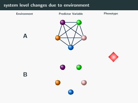
system level changes due to environment
Predictor Variable PhenotypeEnvironment
A
B
Test 1
4

system level changes due to environment
Predictor Variable PhenotypeEnvironment
A
B
Test 1
4

Motivating Dataset: Newborn epigenetic adaptations to gesta-
tional diabetes exposure (Luigi Bouchard, Sherbrooke)
Environment
Gestational
Diabetes
Large Data
Child’s epigenome
(p ≈ 450k)
Phenotype
Obesity measures
5

Differential Correlation between environments
(a) Gestational diabetes affected pregnancy (b) Controls
6

Gene Expression: COPD patients
(a) Gene Exp.: Never Smokers (b) Gene Exp.: Current Smokers
(c) Correlations: Never Smokers (d) Correlations: Current Smokers
7

Imaging Data: Topological properties and Age
8

Correlations differ between Age groups
9

NIH MRI brain study
Environment
Age
Large Data
Cortical Thickness
(p ≈ 80k)
Phenotype
Intelligence
10

Differential Networking
11

formal statement of initial problem
• n: number of subjects
• p: number of predictor variables
• Xn×p: high dimensional data set (p >> n)
• Yn×1: phenotype
• En×1: environmental factor that has widespread effect on X and can
modify the relation between X and Y
Objective
• Which elements of X that are associated with Y , depend on E?
12

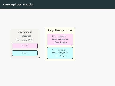
conceptual model
Environment
ff(Maternal
care, Age, Diet)
E = 0
E = 1
Large Data (p >> n)
Gene Expression t
DNA Methylation
t Brain Imaging
Gene Expression t
DNA Methylation
t Brain Imaging
Phenotype (Behavioral
development, IQ
scores, Death)
13
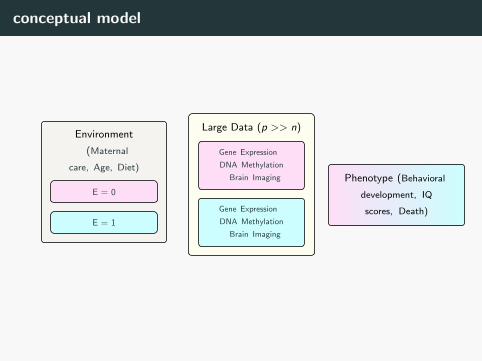
conceptual model
Environment
ff(Maternal
care, Age, Diet)
E = 0
E = 1
Large Data (p >> n)
Gene Expression t
DNA Methylation
t Brain Imaging
Gene Expression t
DNA Methylation
t Brain Imaging
Phenotype (Behavioral
development, IQ
scores, Death)
13
conceptual model
Environment
ff(Maternal
care, Age, Diet)
E = 0
E = 1
Large Data (p >> n)
Gene Expression t
DNA Methylation
t Brain Imaging
Gene Expression t
DNA Methylation
t Brain Imaging
Phenotype (Behavioral
development, IQ
scores, Death)
13

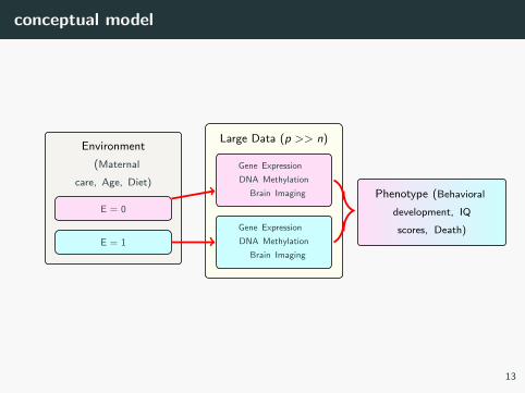
conceptual model
Environment
ff(Maternal
care, Age, Diet)
E = 0
E = 1
Large Data (p >> n)
Gene Expression t
DNA Methylation
t Brain Imaging
Gene Expression t
DNA Methylation
t Brain Imaging
Phenotype (Behavioral
development, IQ
scores, Death)
epidemiological study
13

conceptual model
Environment
ff(Maternal
care, Age, Diet)
E = 0
E = 1
Large Data (p >> n)
Gene Expression t
DNA Methylation
t Brain Imaging
Gene Expression t
DNA Methylation
t Brain Imaging
Phenotype (Behavioral
development, IQ
scores, Death)
(epi)genetic/imaging associations
13

conceptual model
Environment
ff(Maternal
care, Age, Diet)
E = 0
E = 1
Large Data (p >> n)
Gene Expression t
DNA Methylation
t Brain Imaging
Gene Expression t
DNA Methylation
t Brain Imaging
Phenotype (Behavioral
development, IQ
scores, Death)
(epi)genetic/imaging associations
(epi)genetic/imaging associations
13
conceptual model
Environment
ff(Maternal
care, Age, Diet)
E = 0
E = 1
Large Data (p >> n)
Gene Expression t
DNA Methylation
t Brain Imaging
Gene Expression t
DNA Methylation
t Brain Imaging
Phenotype (Behavioral
development, IQ
scores, Death)
13
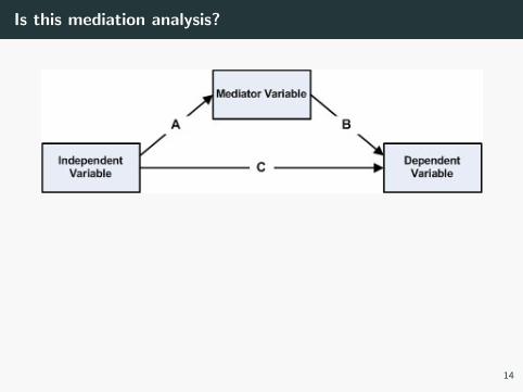
Is this mediation analysis?
• No
• We are not making any causal claims i.e. direction of the arrows
• There are many untestable assumptions required for such analysis
→ not well understood for HD data
14

Is this mediation analysis?
• No
• We are not making any causal claims i.e. direction of the arrows
• There are many untestable assumptions required for such analysis
→ not well understood for HD data
14

Is this mediation analysis?
• No
• We are not making any causal claims i.e. direction of the arrows
• There are many untestable assumptions required for such analysis
→ not well understood for HD data
14

Is this mediation analysis?
• No
• We are not making any causal claims i.e. direction of the arrows
• There are many untestable assumptions required for such analysis
→ not well understood for HD data
14

Methods

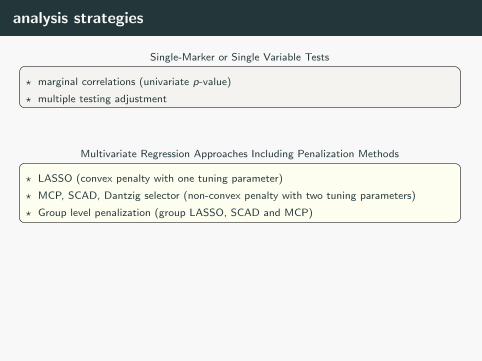
analysis strategies
? marginal correlations (univariate p-value)
? multiple testing adjustment
Single-Marker or Single Variable Tests
? LASSO (convex penalty with one tuning parameter)
? MCP, SCAD, Dantzig selector (non-convex penalty with two tuning parameters)
? Group level penalization (group LASSO, SCAD and MCP)
Multivariate Regression Approaches Including Penalization Methods
? cluster features based on euclidean distance, correlation, connectivity
? regression with group level summary (PCA, average)
Clustering Together with Regression
15

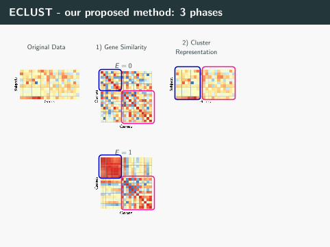
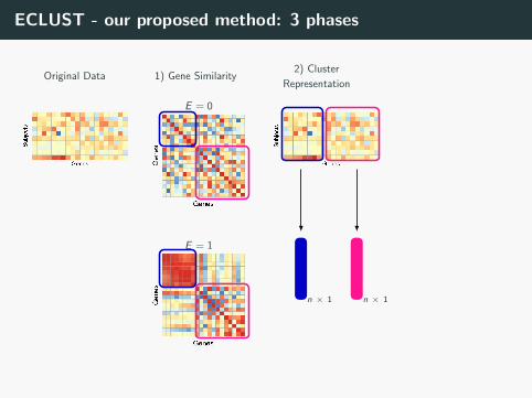
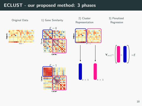
ECLUST - our proposed method: 3 phases
Original Data
E = 0
1) Gene Similarity
E = 1
2) Cluster
Representation
n × 1 n × 1
3) Penalized
Regression
Yn×1∼ + ×E
16

ECLUST - our proposed method: 3 phases
Original Data
E = 0
1) Gene Similarity
E = 1
2) Cluster
Representation
n × 1 n × 1
3) Penalized
Regression
Yn×1∼ + ×E
16

ECLUST - our proposed method: 3 phases
Original Data
E = 0
1) Gene Similarity
E = 1
2) Cluster
Representation
n × 1 n × 1
3) Penalized
Regression
Yn×1∼ + ×E
16
ECLUST - our proposed method: 3 phases
Original Data
E = 0
1) Gene Similarity
E = 1
2) Cluster
Representation
n × 1 n × 1
3) Penalized
Regression
Yn×1∼ + ×E
16
ECLUST - our proposed method: 3 phases
Original Data
E = 0
1) Gene Similarity
E = 1
2) Cluster
Representation
n × 1 n × 1
3) Penalized
Regression
Yn×1∼ + ×E
16

ECLUST - our proposed method: 3 phases
Original Data
E = 0
1) Gene Similarity
E = 1
2) Cluster
Representation
n × 1 n × 1
3) Penalized
Regression
Yn×1∼ + ×E
16

the objective of statistical
methods is the reduction of data.
A quantity of data . . . is to be
replaced by relatively few quantities
which shall adequately represent
. . . the relevant information
contained in the original data.
- Sir R. A. Fisher, 1922
16

Underlying model
Y = β0 + β1U + β2U · E + ε (1)
X ∼ F (α0 + α1U,ΣE ) (2)
• U: unobserved latent variable
• X : observed data which is a function of U
• ΣE : environment sensitive correlation matrix
17

Underlying model
Y = β0 + β1U + β2U · E + ε (1)
X ∼ F (α0 + α1U,ΣE ) (2)
• U: unobserved latent variable
• X : observed data which is a function of U
• ΣE : environment sensitive correlation matrix
17

Underlying model
Y = β0 + β1U + β2U · E + ε (1)
X ∼ F (α0 + α1U,ΣE ) (2)
• U: unobserved latent variable
• X : observed data which is a function of U
• ΣE : environment sensitive correlation matrix
17
ECLUST - our proposed method: 3 phases
Original Data
E = 0
1) Gene Similarity
E = 1
2) Cluster
Representation
n × 1 n × 1
3) Penalized
Regression
Yn×1∼ + ×E
18

advantages and disadvantages
General Approach Advantages Disadvantages
Single-Marker simple, easy to implementmultiple testing burden,
power, interpretability
Penalization
multivariate, variable
selection, sparsity, efficient
optimization algorithms
poor sensitivity with
correlated data, ignores
structure in design matrix,
interpretability
Environment Cluster with
Regression
multivariate, flexible
implementation,
group structure, takes
advantage of correlation,
interpretability
difficult to identify relevant
clusters, clustering is
unsupervised
19

Methods to detect gene clusters
Table 1: Methods to detect gene clusters
General Approach Formula
Correlationpearson, spearman,
biweight midcorrelation
Correlation Scoring |ρE=1 − ρE=0|
Weighted Correlation
Scoringc|ρE=1 − ρE=0|
Fisher’s Z
Transformation
|zij0−zij1|√1/(n0−3)+1/(n1−3)
20
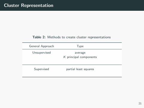
Cluster Representation
Table 2: Methods to create cluster representations
General Approach Type
Unsupervised average
K principal components
Supervised partial least squares
21

Simulation Studies

Simulation Study 1
(a) Corr(XE=0) (b) Corr(XE=1)
(c) |Corr(XE=1)− Corr(XE=0)| (d) Corr(Xall)22
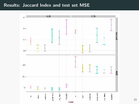
Results: Jaccard Index and test set MSE
23
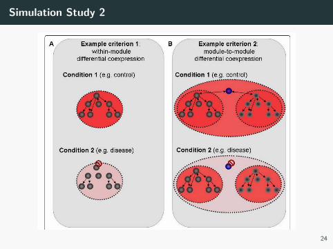
Simulation Study 2
24

TOM based on all subjects
(a) TOM(Xall)25

TOM based on unexposed subjects
(a) TOM(XE=0)26

TOM based on exposed subjects
(a) TOM(XE=1)27

Difference of TOMs
(a) |TOM(XE=1)− TOM(XE=0)|28

Results: Test set MSE
29

Strong Heredity Models

Model
g(µ) =β0 + β1X1 + · · ·+ βpXp + βEE︸ ︷︷ ︸main effects
+α1E (X1E ) + · · ·+ αpE (XpE )︸ ︷︷ ︸interactions
• g(·) is a known link function
• µ = E [Y |X,E ,β,α]
• β = (β1, β2, . . . , βp, βE ) ∈ Rp+1
• α = (α1E , . . . , αpE ) ∈ Rp
30

Variable Selection
arg minβ0,β,α
1
2‖Y − g(µ)‖2 + λ (‖β‖1 + ‖α‖1)
• ‖Y − g(µ)‖2 =∑
i (yi − g(µi ))2
• ‖β‖1 =∑
j |βj |• ‖α‖1 =
∑j |αj |
• λ ≥ 0: tuning parameter
31

Why Strong Heredity?
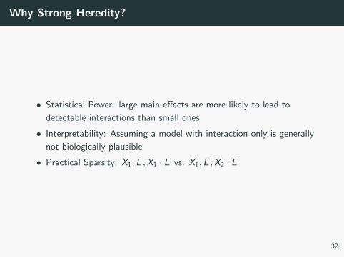
• Statistical Power: large main effects are more likely to lead to
detectable interactions than small ones
• Interpretability: Assuming a model with interaction only is generally
not biologically plausible
• Practical Sparsity: X1,E ,X1 · E vs. X1,E ,X2 · E
32

Why Strong Heredity?
• Statistical Power: large main effects are more likely to lead to
detectable interactions than small ones
• Interpretability: Assuming a model with interaction only is generally
not biologically plausible
• Practical Sparsity: X1,E ,X1 · E vs. X1,E ,X2 · E
32
Why Strong Heredity?
• Statistical Power: large main effects are more likely to lead to
detectable interactions than small ones
• Interpretability: Assuming a model with interaction only is generally
not biologically plausible
• Practical Sparsity: X1,E ,X1 · E vs. X1,E ,X2 · E
32
Model
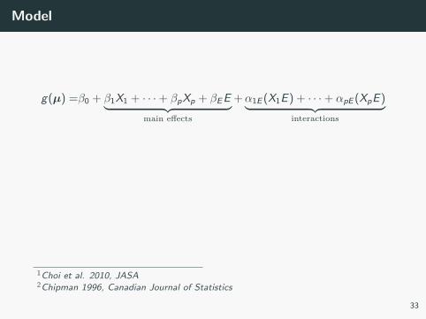
g(µ) =β0 + β1X1 + · · ·+ βpXp + βEE︸ ︷︷ ︸main effects
+α1E (X1E ) + · · ·+ αpE (XpE )︸ ︷︷ ︸interactions
Reparametrization1: αjE = γjEβjβE .
Strong heredity principle2:
αjE 6= 0 ⇒ βj 6= 0 and βE 6= 0
1Choi et al. 2010, JASA2Chipman 1996, Canadian Journal of Statistics
33

Model
g(µ) =β0 + β1X1 + · · ·+ βpXp + βEE︸ ︷︷ ︸main effects
+α1E (X1E ) + · · ·+ αpE (XpE )︸ ︷︷ ︸interactions
Reparametrization1: αjE = γjEβjβE .
Strong heredity principle2:
αjE 6= 0 ⇒ βj 6= 0 and βE 6= 0
1Choi et al. 2010, JASA2Chipman 1996, Canadian Journal of Statistics
33

Model
g(µ) =β0 + β1X1 + · · ·+ βpXp + βEE︸ ︷︷ ︸main effects
+α1E (X1E ) + · · ·+ αpE (XpE )︸ ︷︷ ︸interactions
Reparametrization1: αjE = γjEβjβE .
Strong heredity principle2:
αjE 6= 0 ⇒ βj 6= 0 and βE 6= 0
1Choi et al. 2010, JASA2Chipman 1996, Canadian Journal of Statistics
33

Strong Heredity Model with Penalization
arg minβ0,β,γ
1
2‖Y − g(µ)‖2 +
λβ (w1β1 + · · ·+ wqβq + wEβE ) +
λγ (w1Eγ1E + · · ·+ wqEγqE )
wj =
∣∣∣∣∣ 1
βj
∣∣∣∣∣ , wjE =
∣∣∣∣∣ βj βEαjE
∣∣∣∣∣
34

Open source software
• Software implementation in R: http://sahirbhatnagar.com/eclust/
• Allows user specified interaction terms
• Automatically determines the optimal tuning parameters through
cross validation
• Can also be applied to genetic data (SNPs)
35

Feature Screening and
Non-linear associations

The most popular way of feature screening
How to fit statistical models when you have over 100,000 features?
Marginal correlations, t-tests
• for each feature, calculate the correlation between X and Y
• keep all features with correlation greater than some threshold
• However this procedure assumes a linear relationship between X and
Y
36

The most popular way of feature screening
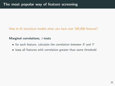
How to fit statistical models when you have over 100,000 features?
Marginal correlations, t-tests
• for each feature, calculate the correlation between X and Y
• keep all features with correlation greater than some threshold
• However this procedure assumes a linear relationship between X and
Y
36
The most popular way of feature screening
How to fit statistical models when you have over 100,000 features?
Marginal correlations, t-tests
• for each feature, calculate the correlation between X and Y
• keep all features with correlation greater than some threshold
• However this procedure assumes a linear relationship between X and
Y
36

Non-linear feature screening: Kolmogorov-Smirnov Test
Mai & Zou (2012) proposed using the Kolmogorov-Smirnov (KS) test
statistic
Kj = supx|Fj(x |Y = 1)− Fj(x |Y = 0)| (3)
Figure 8: Depiction of KS statistic
37

Non-linear Interaction Models
After feature screening, we can fit non-linear relationships between
X and Y
Yi = β0 +∑
f (Xij) +∑
f (Xij ,Ei ) + εi (4)
38

Conclusions

Conclusions and Contributions
• Large system-wide changes are observed in many environments
• This assumption can possibly be exploited to aid analysis of large
data
• We develop and implement a multivariate penalization procedure for
predicting a continuous or binary disease outcome while detecting
interactions between high dimensional data (p >> n) and an
environmental factor.
• Dimension reduction is achieved through leveraging the
environmental-class-conditional correlations
• Also, we develop and implement a strong heredity framework
within the penalized model
• R software: http://sahirbhatnagar.com/eclust/
39

Limitations
• There must be a high-dimensional signature of the exposure
• Clustering is unsupervised
• Two tuning parameters
40

Limitations
• There must be a high-dimensional signature of the exposure
• Clustering is unsupervised
• Two tuning parameters
40
Limitations
• There must be a high-dimensional signature of the exposure
• Clustering is unsupervised
• Two tuning parameters
40

What type of data is required to
use these methods
ECLUST method
1. environmental exposure (currently only binary)
2. a high dimensional dataset that can be affected by the exposure
3. a single phenotype (continuous or binary)
4. Must be a high-dimensional signature of the exposure
41

Strong Heredity and Non-linear Models
1. a single phenotype (continuous or binary)
2. environment variable (continuous or binary)
3. any number of predictor variables
42

Check out our Lab’s Software!
http://greenwoodlab.github.io/software/
43

acknowledgements
• Dr. Celia Greenwood
• Dr. Blanchette and Dr. Yang
• Dr. Luigi Bouchard, Andre Anne
Houde
• Dr. Steele, Dr. Kramer,
Dr. Abrahamowicz
• Maxime Turgeon, Kevin
McGregor, Lauren Mokry,
Marie Forest, Pablo Ginestet
• Greg Voisin, Vince Forgetta,
Kathleen Klein
• Mothers and children from the
study
44