Introduction to Simulation - Lecture 15

Thanks to Deepak Ramaswamy, Michal Rewienski, and Karen Veroy

Methods for Computing Periodic Steady-State

Jacob White

Outline

• Periodic Steady-state problems– Application examples and simple cases

• Finite-difference methods– Formulating large matrices

• Shooting Methods– State transition function

– Sensitivity matrix

• Matrix Free Approach

SMA-HPC ©2003 MIT

Basic DefinitionPeriodic Steady-State Basics

• Suppose the system has a periodic input

• Many Systems eventually respond periodically

( ) ( ){ {( )

inputstate

dx tF x t u t

dt

= +

( ) ( ) 0x t T x t for t+ = >>

tT 2T 3T

SMA-HPC ©2003 MIT

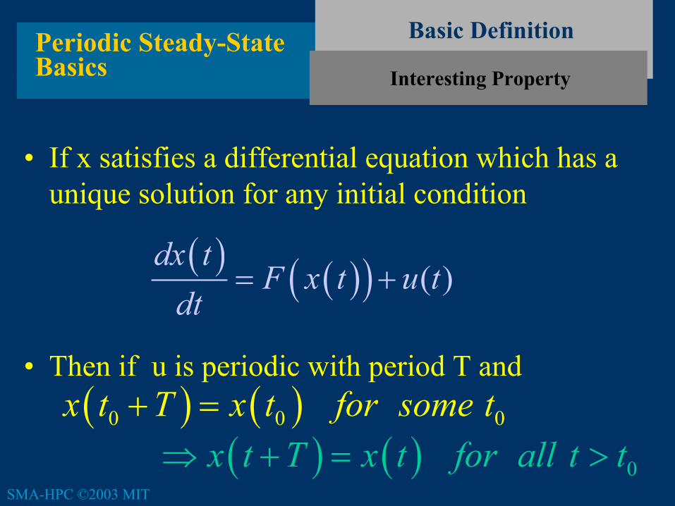
Basic DefinitionPeriodic Steady-State Basics

• If x satisfies a differential equation which has a unique solution for any initial condition

• Then if u is periodic with period T and

( ) ( )( ) ( )dx t

F x t u tdt

= +

( ) ( )0 0 0x t T x t for some t+ =

Interesting Property

( ) ( ) 0x t T x t for all t t⇒ + = >

SMA-HPC ©2003 MIT

Application ExamplesPeriodic Steady-State Basics

• Periodic Input– Wind

• Response– Oscillating Platform

• Desired Info– Oscillation Amplitude

Swaying Bridge

SMA-HPC ©2003 MIT

Application ExamplesPeriodic Steady-State Basics Communication Integrated

Circuit

• Periodic Input– Received Signal at 900Mhz

• Response– filtered demodulated signal

• Desired Info– Distortion

SMA-HPC ©2003 MIT

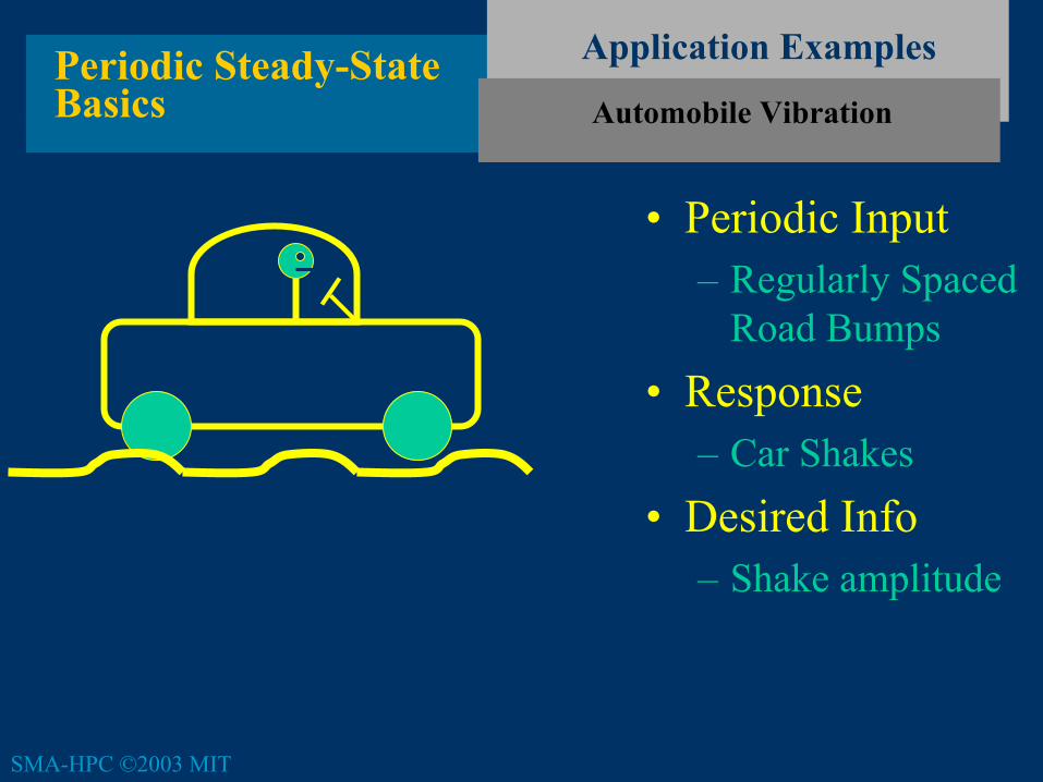
Application ExamplesPeriodic Steady-State Basics Automobile Vibration

• Periodic Input– Regularly Spaced

Road Bumps• Response

– Car Shakes• Desired Info

– Shake amplitude

SMA-HPC ©2003 MIT

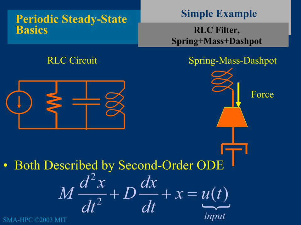
Simple ExamplePeriodic Steady-State Basics RLC Filter,

Spring+Mass+Dashpot

Spring-Mass-DashpotRLC Circuit

• Both Described by Second-Order ODE

Force

{

2

2 ( )input

d x dxM D x u tdt dt

+ + =

SMA-HPC ©2003 MIT

Simple ExamplePeriodic Steady-State Basics RLC Filter,

Spring+Mass+Dashpot Cont.

• Both Described by Second-Order ODE

• u(t) = 0 lightly damped (D<<M) Response

2

2 ( )d x dxM D x u tdt dt

+ + =

( ) 2 cosDM tx t Ke

Mφ

− ≈ +

SMA-HPC ©2003 MIT

Simple ExamplePeriodic Steady-State Basics RLC Filter,

Spring+Mass+Dashpot Cont.

• A lightly damped system oscillates many times before settling to a steady-state

2DMKe

−

SMA-HPC ©2003 MIT

Computing Steady StatePeriodic Steady-State Basics

Frequency Domain Approach

• Sinusoidally excited linear time-invariant system

• Steady-State Solution simple to determine

( ) ( ) {i tinput

dx tAx t e

dtω= +

( ) ( ) 1 i tx t i A e ωω −= −Not useful for nonlinear or time-varying systems

SMA-HPC ©2003 MIT

Computing Steady StatePeriodic Steady-State Basics

Time Integration Method

• Time-Integrate Until Steady-State Achieved

• Need many timepoints for lightly damped case!

( ) ( )( ) ( )( )1ˆ ˆ ˆ( ) ( )l l ldx tF x t u t x x t F x u l t

dt−= + ⇒ = + ∆ + ∆

SMA-HPC ©2003 MIT

Solve with Backward-EulerAside Reviewing Integration Methods

• Nonlinear System

• Backward Euler Equation for timestep l

( ) ( ){ { ( ) 0( 0)

inp InitialCondutstate ition

xdx t

F x t u t xdt

= +

=14243

( )( )1ˆ ˆ ˆ ( )l l lx x t F x u l t−− = ∆ + ∆

How do we solve the backward-Euler Equation?

SMA-HPC ©2003 MIT

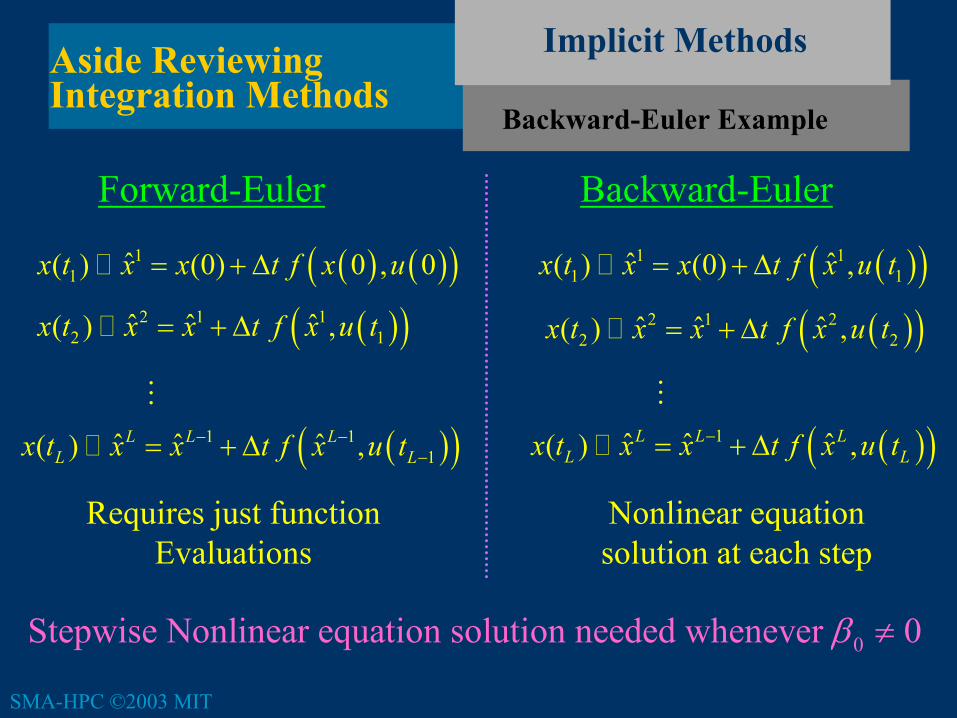
( ) ( )( )11 ˆ( ) (0) 0 , 0x t x x t f x u= + ∆

( )( )2 1 12 1ˆ ˆ ˆ( ) ,x t x x t f x u t= + ∆

( )( )1 11ˆ ˆ ˆ( ) ,L L L

L Lx t x x t f x u t− −−= + ∆

M

Forward-Euler

Requires just functionEvaluations

Backward-Euler

( )( )1 11 1ˆ ˆ( ) (0) ,x t x x t f x u t= + ∆

( )( )2 1 22 2ˆ ˆ ˆ( ) ,x t x x t f x u t= + ∆

( )( )1ˆ ˆ ˆ( ) ,L L LL Lx t x x t f x u t−= + ∆

M

Nonlinear equationsolution at each step

0Stepwise Nonlinear equation solution needed whenever 0β ≠

Backward-Euler Example

Implicit MethodsAside Reviewing Integration Methods

SMA-HPC ©2003 MIT

Solution with Newton

Implicit Methods

( )( ) ( )( )1 1

0 0 ˆ ˆ ,ˆ ˆ , 0l lk k

l j l jj j j

j jl lxx t f x u t f x ut tα βα β − −

−= =

=∆∆ + −− ∑ ∑Rewrite the multistep Equation

b ˆIndependent of lxSolve with Newton( )( ) ( ) ( )( )( )

,, 1 , , ,

0 0 0 0

ˆ ,ˆ ˆ ˆ ˆ ,

l jl l j l j l j l j

l

f x u tI t x x x t f x u t b

xα β α β+ ∂ − ∆ − = − −∆ + ∂

Here j is the Newton iteration index

Jacobian ( ),l jF x

Aside Reviewing Integration Methods

SMA-HPC ©2003 MIT

Newton Iteration: ( )( ) ( ),

, 1 , ,0 0

ˆ ,ˆ ˆ ( )

l jl l j l j l j

f x u tI t x x F x

xα β + ∂ − ∆ − = − ∂

Solution with Newton is very efficient

lt1lt −2lt −3lt −l kt −

Easy to generate a good initial guess using polynomial fitting

,0ˆ lx

Polynomial Predictor

ˆ lxConverged

Solution

( )( )0

,

0 0

ˆ ,as 0

l jlf x u

It

I t tx

α β α∂

−∆ ∆ →∂

⇒Jacobian become easy to factor for small timesteps

Solution with Newton Cont.

Implicit MethodsAside Reviewing Integration Methods

SMA-HPC ©2003 MIT

Basic FormulationBoundary-Value Problem

Differential Equation Solution

Periodicity Constraint

( ) ( )( )N Differential Equations: i id x t F x tdt

=

( ) ( )N Periodicity Cons traints: 0i ix T x=

SMA-HPC ©2003 MIT

Finite Difference MethodsBoundary-Value Problem

Linear Example Problem

( ) ( ) ( ){

[ ] ( ) ( )periodicity constraint

0,input

dx tAx t u t t T x T x t

dt= + ∈ =

14243

Discretize with Backward-Euler( )( )1 0 1ˆ ˆ ˆx x t Ax u t= + ∆ + ∆( )( )2 1 2ˆ ˆ ˆ 2x x t Ax u t= + ∆ + ∆

( )( )1ˆ ˆ ˆL L Lx x t Ax u L t−= + ∆ + ∆

TtL

∆ =

0Periodicity im ˆ ˆ plies Lx x=

SMA-HPC ©2003 MIT

Finite Difference MethodsBoundary-Value Problem

Linear Example Matrix Form

( )( )

( )

1

2

1 10 0 0ˆˆ1 1 0 0

0 01 1 ˆ0 0

L

I A I uxt tu tx

I I At t

u L txI I At t

− − ∆ ∆ ∆ − − =∆ ∆ ∆ − − ∆ ∆

MM

O O MM

Matrix is almost lower triangular

NxL

NxL

SMA-HPC ©2003 MIT

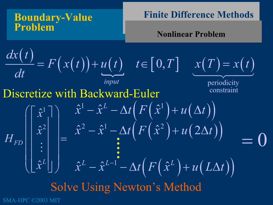
Finite Difference MethodsBoundary-Value Problem

Nonlinear Problem

( ) ( )( ) ( ){

[ ] ( ) ( )periodicity constraint

0,input

dx tF x t u t t T x T x t

dt= + ∈ =

14243

Discretize with Backward-Euler( ) ( )( )1 1ˆ ˆ ˆLx x t F x u t− −∆ + ∆

( ) ( )( )2 1 2ˆ ˆ ˆ 2x x t F x u t− − ∆ + ∆

( ) ( )( )1ˆ ˆ ˆL L Lx x t F x u L t−− − ∆ + ∆

1

2

ˆˆ

ˆ

FD

L

xx

H

x

=

M 0=

Solve Using Newton’s Method

SMA-HPC ©2003 MIT

Shooting MethodBoundary-Value Problem

Basic Definitions

( ) ( )( ) ( )dx tF x t u t

dt= +Start with

And assume x(t) is unique given x(0).

D.E. defines a State-Transition Function

( ) ( )0 1 1, ,y t t x tΦ ≡

( )0where ( ) is the D.E. solution given x t x t y=

SMA-HPC ©2003 MIT

Shooting MethodBoundary-Value Problem State Transition function Example

( ) ( )dx tx t

dtλ=

( ) ( )1 00 1, , t ty t t e yλ −Φ ≡

SMA-HPC ©2003 MIT

Shooting MethodBoundary-Value Problem

Abstract Formulation

Solve

Use Newton’s method

( )( ) ( )( )( )

( )0 0 ,0, 0 0H x x T x

x T

= Φ − =1442443

( ) ( ),0,H

x TJ x I

x∂Φ

= −∂

( )( ) ( )1k k k kHJ x x x H x+ − = −

SMA-HPC ©2003 MIT

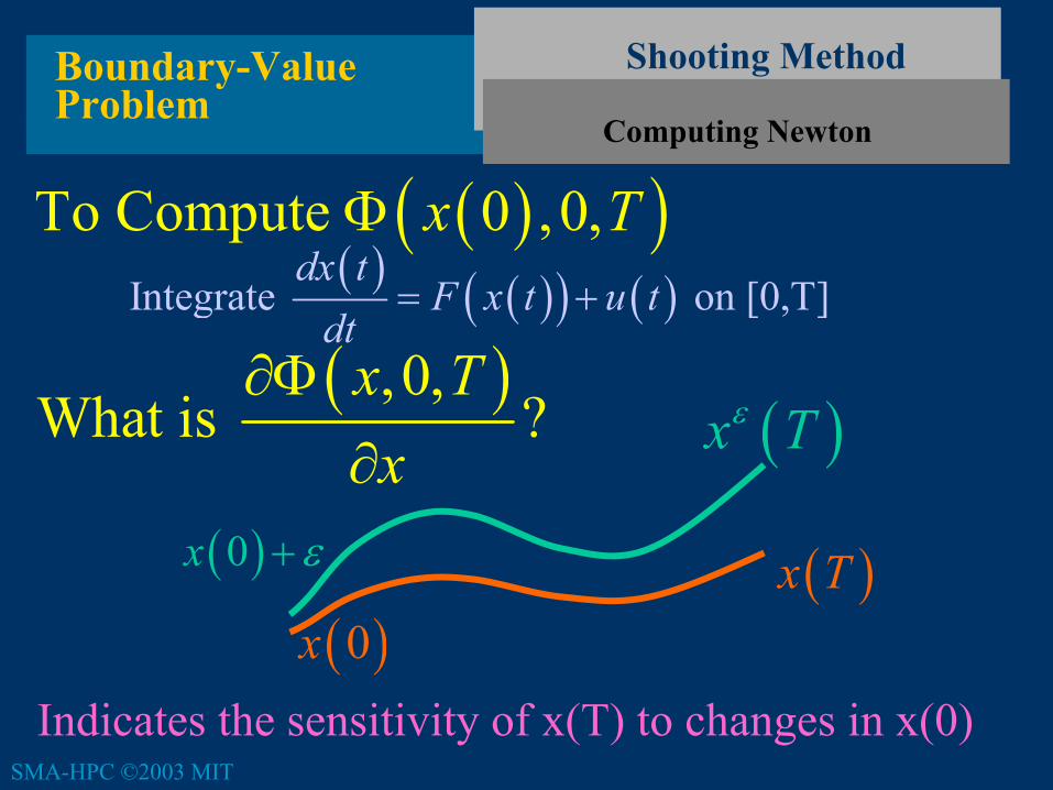
Shooting MethodBoundary-Value Problem

Computing Newton

( )( )To Compute 0 ,0,x TΦ

( ),0,What is ?

x Tx

∂Φ∂

( ) ( )( ) ( )Integrate on [0,T]dx t

F x t u tdt

= +

( )0x ε+

( )0x( )x T

( )x Tε

Indicates the sensitivity of x(T) to changes in x(0)

SMA-HPC ©2003 MIT

Shooting MethodBoundary-Value Problem Sensitivity Matrix by Perturbation

( ) ( ) ( ) ( )

( ) ( ) ( ) ( )

1

1

1 1 1 1

1

1

N

N

N

N N N N

N

x T x T x T x T

x T x T x T x T

εε

εε

ε ε

ε ε

− − − −

L L

M L L M

M L L M

L L

( ),0,x Tx

∂Φ≈

∂

SMA-HPC ©2003 MIT

Shooting MethodBoundary-Value Problem Efficient Sensitivity Evaluation

( ) ( ) ( ) ( )( )( )1 10 00

ˆ ˆx x ux

t F x t− −∆ + ∆∂

=∂

Differentiate the first step of Backward-Euler

( )( )( )

( )( )

11 100

ˆˆ0

0ˆ0

F xx xtx

x x x x∂∂∂ ∂

⇒ −∂ ∂ ∂ ∂

− ∆ =

I( )( )

( )( )

1 1 00 0

ˆ ˆF xt

xx x

xIx

∂ ∂∂ ⇒ ∂ ∂ ∂

− ∆ =

SMA-HPC ©2003 MIT

Shooting MethodBoundary-Value Problem Efficient Sensitivity Matrix Cont

( )( ) ( )

1ˆ ˆ0

ˆ0

l l l

Ix x x

F x x xt− ∂ ∂ ∂ ⇒

∂ ∂ ∂ − ∆ =

Applying the same trick on the l-th step

( ),0,x Tx

∂Φ≈

∂

( ) 1

1

ˆ lL

l

Ix

F xt

−

=

∂ ∂

− ∆∏

SMA-HPC ©2003 MIT

Shooting MethodBoundary-Value Problem Observations on Sensitivity Matrix

Newton at each timestep uses same matrices

( ),0,x Tx

∂Φ≈

∂

( ) 1

1

ˆL

l

Timestep NewtonJacobian

l

Ix

F xt

−

=

∂

−

∆∂∏

1442443

Formula simplifies in the linear case( ),0,x Tx

∂Φ≈

∂( ) LI tA −− ∆

SMA-HPC ©2003 MIT

Matrix-Free ApproachShooting Method

Basic Setup

Start with ( ) ( )( ) ( )dx t

F x t u tdt

= +

Use Newton’s method

( )( ) ( )( ) ( )0 0 ,0, 0 0H x x T x= Φ − =

( ) ( ),0,H

x TJ x I

x∂Φ

= −∂

( )( ) ( )1k k k kHJ x x x H x+ − = −

SMA-HPC ©2003 MIT

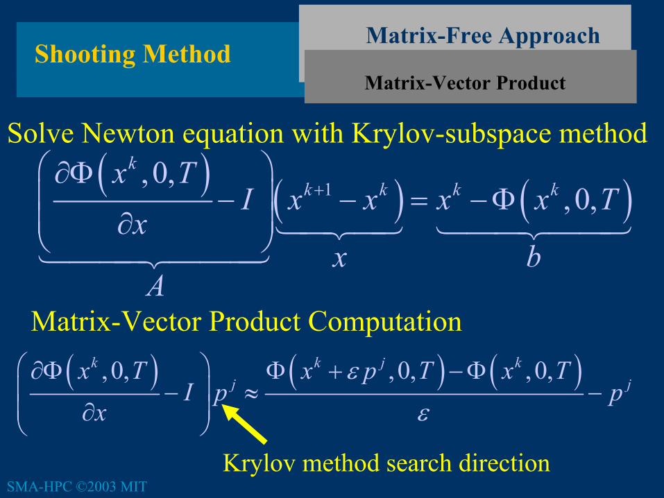
Matrix-Free ApproachShooting Method

Matrix-Vector Product

( ) ( ) ( )1,0,

,0,k

k k k kx T

I x x x x Tx

x bA

+ ∂Φ − − = −Φ ∂ 14243 1442443144424443

Solve Newton equation with Krylov-subspace method

Matrix-Vector Product Computation

( ) ( ) ( ),0, ,0, ,0,k k j kj j

x T x p T x TI p p

xε

ε

∂Φ Φ + −Φ − ≈ − ∂

Krylov method search direction

SMA-HPC ©2003 MIT

Matrix-Free ApproachShooting Method

Convergence for GCR

Example

Shooting-Newton Jacobian

( )0 real and negativedx Ax eig Adt

− =

( ),0, ATx TI e I

x∂Φ

− = −∂

SMA-HPC ©2003 MIT

Matrix-Free ApproachShooting Method

Convergence for GCR-evals

1

1

1

1N

T

AT

T

ee I S S

e

λ

λ

−

− − = −

O

1

Many Fast Modes cluster at 1

Few Slow Modes larger than 1

Summary

• Periodic Steady-state problems– Application examples and simple cases

• Finite-difference methods– Formulating large matrices

• Shooting Methods– State transition function

– Sensitivity matrix