Lecture 1 Sujin Khomrutai – 1 / 27

Method of Applied MathLecture 2: Legendre’s Equation and Legendre

Polynomials

Sujin Khomrutai, Ph.D.

Legendre’s equation

Legendre’s eqn

EX 1.

Series Sol

Legendre func

Rodrigues’ form

EX 2.

EX 3.

Gamma function

Properties

EX 4.

EX 5.

EX 6.

EX 7.

Lecture 1 Sujin Khomrutai – 2 / 27

Definition Let n be a constant. The ODE of the form

(1− x2)y′′ − 2xy′ + n(n+ 1)y = 0

is called the Legendre equation of order n.

• n = 0: (1− x2)y′′ − 2xy′ = 0

• n = 1: (1− x2)y′′ − 2xy′ + 2y = 0

• n = 2: (1− x2)y′′ − 2xy′ + 6y = 0

• n = 3: (1− x2)y′′ − 2xy′ + 12y = 0

In theory, n can be any real number, however, real phenomenashow non-negative integer n. We restrict to the latter case.

Example 1: (Electrostatics)

Legendre’s eqn

EX 1.

Series Sol

Legendre func

Rodrigues’ form

EX 2.

EX 3.

Gamma function

Properties

EX 4.

EX 5.

EX 6.

EX 7.

Lecture 1 Sujin Khomrutai – 3 / 27

Example. A two metallic spherical caps are placed so that theupper part stayed at a constant potential 110 V and the lowerpart is grounded. The electrostatic potential at any point in thespace can be calculated by solving the Legendre’s equation.

Series solutions of Legendre’s equation

Legendre’s eqn

EX 1.

Series Sol

Legendre func

Rodrigues’ form

EX 2.

EX 3.

Gamma function

Properties

EX 4.

EX 5.

EX 6.

EX 7.

Lecture 1 Sujin Khomrutai – 4 / 27

Power series method. a = 0 is an ordinary point. Set solutiony to the Legendre’s equation

(1− x2)y′′ − 2xy′ + n(n+ 1)y = 0,

as

y =∞∑

k=0

bkxk

y′ =∞∑

k=0

bk+1(k + 1)xk

y′′ =∞∑

k=0

bk+2(k + 2)(k + 1)xk.

Series solutions of Legendre’s equation

Legendre’s eqn

EX 1.

Series Sol

Legendre func

Rodrigues’ form

EX 2.

EX 3.

Gamma function

Properties

EX 4.

EX 5.

EX 6.

EX 7.

Lecture 1 Sujin Khomrutai – 5 / 27

The first term

(1− x2)y′′ = y′′ − x2y′′

=∞∑

k=0

bk+2(k + 2)(k + 1)xk −∞∑

k=0

bk+2(k + 2)(k + 1)xk+2

=∞∑

k=0

bk+2(k + 2)(k + 1)xk −∞∑

j=2

bjj(j − 1)xj

= b2 · 2 · 1 + b3 · 3 · 2x

+∞∑

k=2

[bk+2(k + 2)(k + 1)− bkk(k − 1)]xk

where we have use shifting and splitting.

Series solutions of Legendre’s equation

Legendre’s eqn

EX 1.

Series Sol

Legendre func

Rodrigues’ form

EX 2.

EX 3.

Gamma function

Properties

EX 4.

EX 5.

EX 6.

EX 7.

Lecture 1 Sujin Khomrutai – 6 / 27

The second term

2xy′ = 2x∞∑

k=0

bk+1(k + 1)xk

=∞∑

k=0

2bk+1(k + 1)xk+1

=∞∑

k=1

2bkkxk

Third term

n(n+ 1)y = n(n+ 1)∞∑

k=0

bkxk =

∞∑

k=0

n(n+ 1)bkxk

Series solutions of Legendre’s equation

Legendre’s eqn

EX 1.

Series Sol

Legendre func

Rodrigues’ form

EX 2.

EX 3.

Gamma function

Properties

EX 4.

EX 5.

EX 6.

EX 7.

Lecture 1 Sujin Khomrutai – 7 / 27

Thus

b2 · 2 · 1 + b3 · 3 · 2x

+∞∑

k=2

[bk+2(k + 2)(k + 1)− bkk(k − 1)]xk

−∞∑

k=1

2bkkxk +

∞∑

k=0

n(n + 1)bkxk = 0

∴ [2b2 + n(n+ 1)b0] + [6b3 − 2b1 + n(n+ 1)b1]x

+∞∑

k=2

[bk+2(k + 2)(k + 1)− bkk(k − 1)

− 2bkk + n(n+ 1)bk]xk = 0

Series solutions of Legendre’s equation

Legendre’s eqn

EX 1.

Series Sol

Legendre func

Rodrigues’ form

EX 2.

EX 3.

Gamma function

Properties

EX 4.

EX 5.

EX 6.

EX 7.

Lecture 1 Sujin Khomrutai – 8 / 27

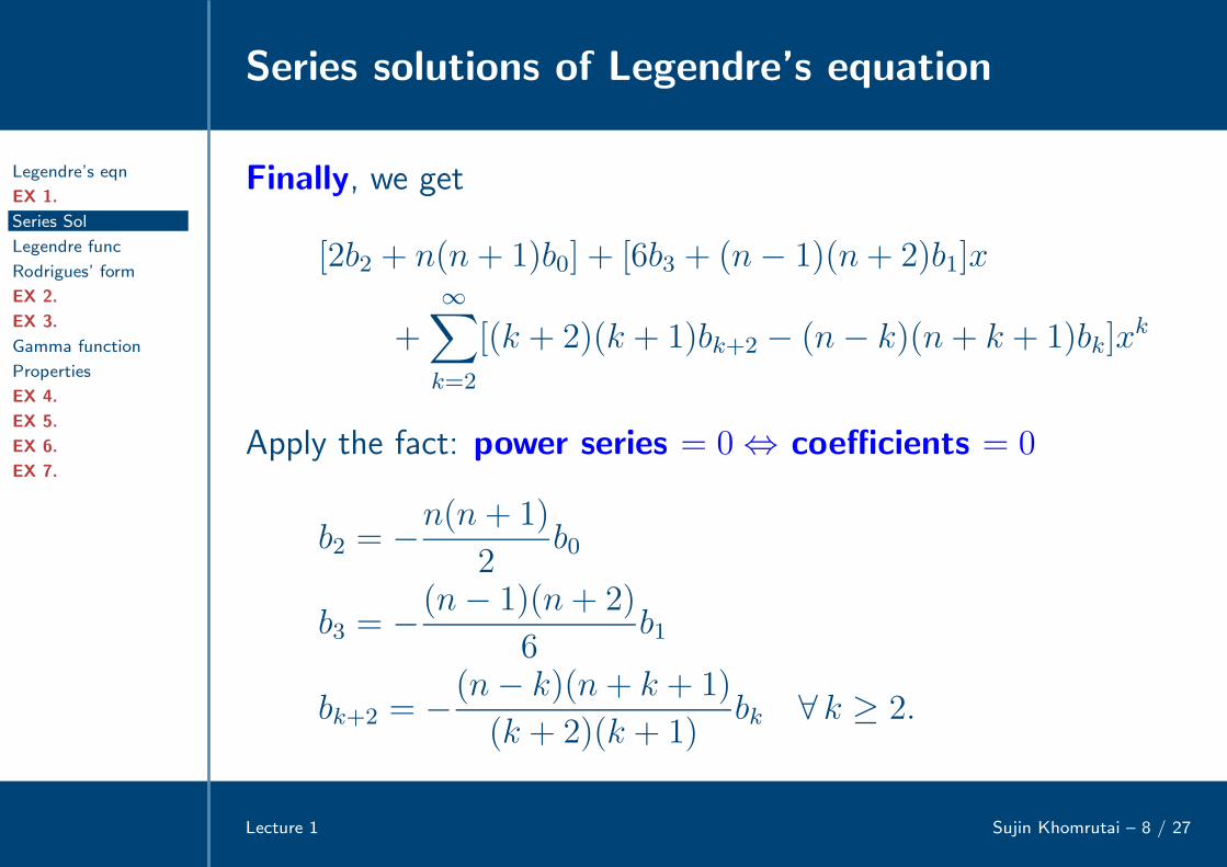
Finally, we get

[2b2 + n(n+ 1)b0] + [6b3 + (n− 1)(n+ 2)b1]x

+∞∑

k=2

[(k + 2)(k + 1)bk+2 − (n− k)(n+ k + 1)bk]xk

Apply the fact: power series = 0 ⇔ coefficients = 0

b2 = −n(n+ 1)

2b0

b3 = −(n− 1)(n+ 2)

6b1

bk+2 = −(n− k)(n+ k + 1)

(k + 2)(k + 1)bk ∀ k ≥ 2.

Series solutions of Legendre’s equation

Legendre’s eqn

EX 1.

Series Sol

Legendre func

Rodrigues’ form

EX 2.

EX 3.

Gamma function

Properties

EX 4.

EX 5.

EX 6.

EX 7.

Lecture 1 Sujin Khomrutai – 9 / 27

Simplify the presentation, n = 3. Recurrence equations are

b2 = −3 · 4

2b0, b3 = −

2 · 5

3!b1

bk+2 = −(3− k)(3 + k + 1)

(k + 2)(k + 1)bk ∀ k ≥ 2

k = 2 : b4 = −1 · 6

4 · 3b2 =

1 · 6 · 3 · 4

4!b0

k = 3 : b5 = −0 · 7

5 · 4b3 = 0

k = 4 : b6 = −(−1) · 8

6 · 5b4 = −

(−1) · 8 · 1 · 6 · 3 · 4

6!b0

k = 5 : b7 = −(−2) · 9

7 · 6b5 = 0

Series solutions of Legendre’s equation

Legendre’s eqn

EX 1.

Series Sol

Legendre func

Rodrigues’ form

EX 2.

EX 3.

Gamma function

Properties

EX 4.

EX 5.

EX 6.

EX 7.

Lecture 1 Sujin Khomrutai – 10 / 27

The general solution to Legendre’s equation with n = 3 is

y = b0

[

1−3 · 4

2!x2 +

1 · 6 · 3 · 4

4!x4 + · · ·

]

+ b1

[

x−2 · 5

3!x3

]

The fundamental solutions

y1 = x−2 · 5

3!x3 a polynomial degree 3

y2 = 1−3 · 4

2!x2 +

1 · 6 · 3 · 4

4!x4 + · · · an infinite series.

It is true in general, when n is a non-negative integer.

Legendre functions

Legendre’s eqn

EX 1.

Series Sol

Legendre func

Rodrigues’ form

EX 2.

EX 3.

Gamma function

Properties

EX 4.

EX 5.

EX 6.

EX 7.

Lecture 1 Sujin Khomrutai – 11 / 27

Theorem. Let n ∈ {0, 1, 2, . . .}. The general solutions to theLegendre’s equation

(1− x2)y′′ − 2xy′ + n(n+ 1)y = 0

can be expressed as

y = C1Pn(x) + C2Qn(x)

where Pn(x) is a polynomial of degree n and Qn is an infiniteseries.

• Pn = the Legendre polynomial or the Legendre function ofthe first kind.

• Qn = the Legendre function of the second kind.

Legendre functions

Legendre’s eqn

EX 1.

Series Sol

Legendre func

Rodrigues’ form

EX 2.

EX 3.

Gamma function

Properties

EX 4.

EX 5.

EX 6.

EX 7.

Lecture 1 Sujin Khomrutai – 12 / 27

Legendre functions

Legendre’s eqn

EX 1.

Series Sol

Legendre func

Rodrigues’ form

EX 2.

EX 3.

Gamma function

Properties

EX 4.

EX 5.

EX 6.

EX 7.

Lecture 1 Sujin Khomrutai – 13 / 27

Rodrigues’ formula

Legendre’s eqn

EX 1.

Series Sol

Legendre func

Rodrigues’ form

EX 2.

EX 3.

Gamma function

Properties

EX 4.

EX 5.

EX 6.

EX 7.

Lecture 1 Sujin Khomrutai – 14 / 27

The Legendre polynomial in the case n = 0 can be taken

P0(x) = 1.

In fact, the Legendre’s equation with n = 0 is

(1− x2)y′′ − 2xy′ = 0,

which has y = 1 as a solution. For n ≥ 1, we have:

Rodrigues’ formula If n ∈ {1, 2, 3, . . .} then

Pn(x) =1

2nn!

dn

dxn(x2 − 1)n

Example 2

Legendre’s eqn

EX 1.

Series Sol

Legendre func

Rodrigues’ form

EX 2.

EX 3.

Gamma function

Properties

EX 4.

EX 5.

EX 6.

EX 7.

Lecture 1 Sujin Khomrutai – 15 / 27

EX. Verify Rodigues’ solution formula for n = 1, 2, 3.

n = 1 : P1(x) =1

2

d

dx(x2 − 1) = x

(1− x2)x′′ − 2x · x′ + 2x = 0

(1− x2) · 0− 2x · 1 + 2x = 0 True

n = 2 : P2(x) =1

22 · 2!

d2

dx2(x2 − 1)2

=1

8

d2

dx2(x4 − 2x2 + 1) =

3

2x2 −

1

2

(1− x2)(3

2x2 −

1

2)′′ − 2x(

3

2x2 −

1

2)′ + 6(

3

2x2 −

1

2) = 0

(1− x2) · 3− 2x · 3x+ (9x2 − 3) = 0

(3− 3x2)− 6x2 + (9x2 − 3) = 0 True

Example 2

Legendre’s eqn

EX 1.

Series Sol

Legendre func

Rodrigues’ form

EX 2.

EX 3.

Gamma function

Properties

EX 4.

EX 5.

EX 6.

EX 7.

Lecture 1 Sujin Khomrutai – 16 / 27

n = 3 : P3(x) =1

23 · 3!

d3

dx3(x2 − 1)3

=1

48

d3

dx3(x6 − 3x4 + 3x2 − 1)

=5

2x3 −

3

2x

(1− x2)(5

2x3 −

3

2x)′′ − 2x(

5

2x3 −

3

2x)′ + 12(

5

2x3 −

3

2x) = 0

(1− x2)(15x)− 2x(15

2x2 −

3

2) + (30x3 − 18x) = 0

(15x− 15x3)− (15x3 − 3x) + (30x3 − 18x) = 0 True

Example 3

Legendre’s eqn

EX 1.

Series Sol

Legendre func

Rodrigues’ form

EX 2.

EX 3.

Gamma function

Properties

EX 4.

EX 5.

EX 6.

EX 7.

Lecture 1 Sujin Khomrutai – 17 / 27

EX. Solve the Legendre’s equation

(1− x2)y′′ − 2xy′ + 2y = 0.

Sol. We get a solution P1(x) = x. Use the reduction of order

Q1(x) = P1(x)

∫

1

(P1(x))2e−

∫−2x

1−x2dxdx

= x

∫

1

x2e− ln(1−x2)dx

= x

∫

1

x2(1− x2)dx =

x

2ln

(

1 + x

1− x

)

− 1

∴ y = C1x+ C2

[

x

2ln

(

1 + x

1− x

)

− 1

]

The Gamma function

Legendre’s eqn

EX 1.

Series Sol

Legendre func

Rodrigues’ form

EX 2.

EX 3.

Gamma function

Properties

EX 4.

EX 5.

EX 6.

EX 7.

Lecture 1 Sujin Khomrutai – 18 / 27

The factorials are

0! = 1! = 1

2! = 2 · 1 = 2

3! = 3 · 2 · 1 = 6,

...

n! = n(n− 1)(n− 2) · · · 3 · 2 · 1 (n ≥ 4)

In above n must be a non-negative integer, i.e. 0, 1, 2, . . .

The Gamma function is the function defined for real numbersas well and it gives the factorials for non-negative integers.

The Gamma function

Legendre’s eqn

EX 1.

Series Sol

Legendre func

Rodrigues’ form

EX 2.

EX 3.

Gamma function

Properties

EX 4.

EX 5.

EX 6.

EX 7.

Lecture 1 Sujin Khomrutai – 19 / 27

Definition The Gamma function Γ(x) is defined by

• If x > 0,

Γ(x) =

∫

∞

0

e−ttx−1 dt.

• If x < 0 and x 6= −1,−2, . . .,

Γ(x) =Γ(x+ n)

(x+ n− 1)(x+ n− 2) · · · (x+ 1)x

where n is a positive integer such that x+ n > 0.

The Gamma function

Legendre’s eqn

EX 1.

Series Sol

Legendre func

Rodrigues’ form

EX 2.

EX 3.

Gamma function

Properties

EX 4.

EX 5.

EX 6.

EX 7.

Lecture 1 Sujin Khomrutai – 20 / 27

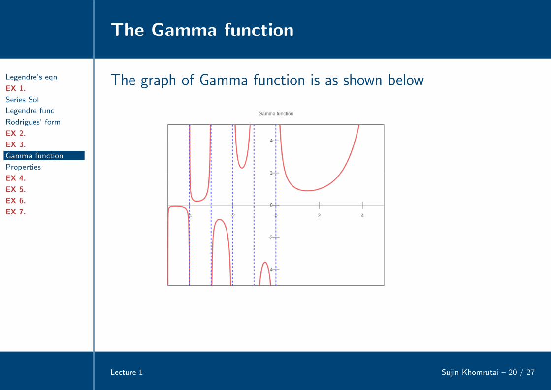
The graph of Gamma function is as shown below

Properties of Gamma function

Legendre’s eqn

EX 1.

Series Sol

Legendre func

Rodrigues’ form

EX 2.

EX 3.

Gamma function

Properties

EX 4.

EX 5.

EX 6.

EX 7.

Lecture 1 Sujin Khomrutai – 21 / 27

(1) Γ(1) = 1. For x > 0,

Γ(x+ 1) = xΓ(x)

(2) Generally, for x > 0 and a positive integer n,

Γ(x+ n) = (x+ n− 1) · · · (x+ 1)xΓ(x) (n ≥ 2).

E.g. Γ(x+2) = (x+1)xΓ(x),Γ(x+3) = (x+2)(x+1)xΓ(x),etc.

(3) For an integer n,

Γ(n+ 1) = n!.

Properties of Gamma function

Legendre’s eqn

EX 1.

Series Sol

Legendre func

Rodrigues’ form

EX 2.

EX 3.

Gamma function

Properties

EX 4.

EX 5.

EX 6.

EX 7.

Lecture 1 Sujin Khomrutai – 22 / 27

Proof. (1) For Γ(1), consider

Γ(1) =

∫

∞

0

e−tt1−1dt =

∫

∞

0

e−tdt

= (−e−t)∣

∣

∣

∞

t=0= 0− (−e0) = 1.

Next, for x > 0 consider

Γ(x+ 1) =

∫

∞

0

e−tt(x+1)−1dt =

∫

∞

0

e−ttxdt

= (−e−ttx)∣

∣

∣

∞

t=0−

∫

∞

0

(−e−txtx−1)dt (by parts)

= x

∫

∞

0

e−ttx−1dt = xΓ(x).

Properties of Gamma function

Legendre’s eqn

EX 1.

Series Sol

Legendre func

Rodrigues’ form

EX 2.

EX 3.

Gamma function

Properties

EX 4.

EX 5.

EX 6.

EX 7.

Lecture 1 Sujin Khomrutai – 23 / 27

(2) For n = 2, we use (1) (x → x+ 1):

Γ(x+ 2) = Γ((x+ 1) + 1) = (x+ 1)Γ(x+ 1),

and then use (1) one more time:

Γ(x+ 1) = xΓ(x).

Thus

Γ(x+ 2) = (x+ 1)xΓ(x)

The argument can be extended to n = 3, n = 4, . . ..

(3) Use x = 1 in (2) and that Γ(1) = 1.

Example 4

Legendre’s eqn

EX 1.

Series Sol

Legendre func

Rodrigues’ form

EX 2.

EX 3.

Gamma function

Properties

EX 4.

EX 5.

EX 6.

EX 7.

Lecture 1 Sujin Khomrutai – 24 / 27

EX. Evaluate

Γ(1) + Γ(4),Γ(2.8)

Γ(0.8).

Example 5

Legendre’s eqn

EX 1.

Series Sol

Legendre func

Rodrigues’ form

EX 2.

EX 3.

Gamma function

Properties

EX 4.

EX 5.

EX 6.

EX 7.

Lecture 1 Sujin Khomrutai – 25 / 27

EX. Evaluate

Γ(−2.5)

in terms of Γ(1.5).

Example 6

Legendre’s eqn

EX 1.

Series Sol

Legendre func

Rodrigues’ form

EX 2.

EX 3.

Gamma function

Properties

EX 4.

EX 5.

EX 6.

EX 7.

Lecture 1 Sujin Khomrutai – 26 / 27

EX. Express

1

(ν + 1)(ν + 2) · · · (ν + n)

as a ratio of Gamma function.

Example 7

Legendre’s eqn

EX 1.

Series Sol

Legendre func

Rodrigues’ form

EX 2.

EX 3.

Gamma function

Properties

EX 4.

EX 5.

EX 6.

EX 7.

Lecture 1 Sujin Khomrutai – 27 / 27

EX. Evaluate the integral

∫

∞

0

t1.35e−tdt.

Express the value in terms of the Gamma function.